mechanical measurements and metrology prof. s. p...

Mechanical Measurements and Metrology Prof. S. P. Venkateshan

Department of Mechanical Engineering Indian Institute of Technology, Madras

Module - 4 Lecture - 39

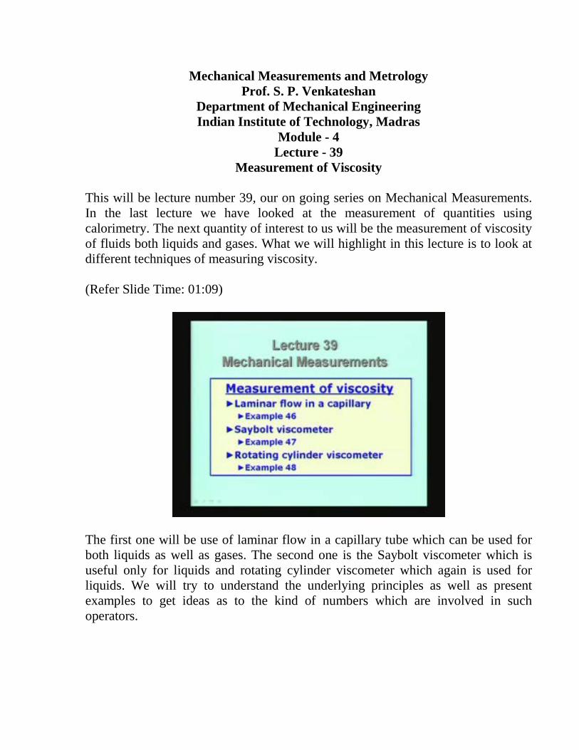
Measurement of Viscosity This will be lecture number 39, our on going series on Mechanical Measurements. In the last lecture we have looked at the measurement of quantities using calorimetry. The next quantity of interest to us will be the measurement of viscosity of fluids both liquids and gases. What we will highlight in this lecture is to look at different techniques of measuring viscosity. (Refer Slide Time: 01:09)

The first one will be use of laminar flow in a capillary tube which can be used for both liquids as well as gases. The second one is the Saybolt viscometer which is useful only for liquids and rotating cylinder viscometer which again is used for liquids. We will try to understand the underlying principles as well as present examples to get ideas as to the kind of numbers which are involved in such operators.

(Refer Slide Time: 02:18)

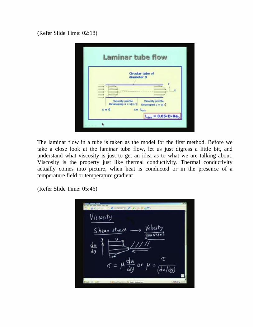
The laminar flow in a tube is taken as the model for the first method. Before we take a close look at the laminar tube flow, let us just digress a little bit, and understand what viscosity is just to get an idea as to what we are talking about. Viscosity is the property just like thermal conductivity. Thermal conductivity actually comes into picture, when heat is conducted or in the presence of a temperature field or temperature gradient. (Refer Slide Time: 05:46)

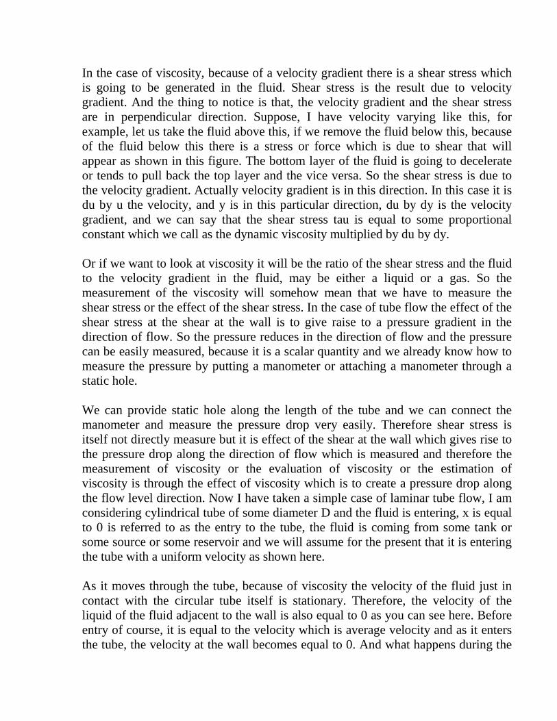
In the case of viscosity, because of a velocity gradient there is a shear stress which is going to be generated in the fluid. Shear stress is the result due to velocity gradient. And the thing to notice is that, the velocity gradient and the shear stress are in perpendicular direction. Suppose, I have velocity varying like this, for example, let us take the fluid above this, if we remove the fluid below this, because of the fluid below this there is a stress or force which is due to shear that will appear as shown in this figure. The bottom layer of the fluid is going to decelerate or tends to pull back the top layer and the vice versa. So the shear stress is due to the velocity gradient. Actually velocity gradient is in this direction. In this case it is du by u the velocity, and y is in this particular direction, du by dy is the velocity gradient, and we can say that the shear stress tau is equal to some proportional constant which we call as the dynamic viscosity multiplied by du by dy. Or if we want to look at viscosity it will be the ratio of the shear stress and the fluid to the velocity gradient in the fluid, may be either a liquid or a gas. So the measurement of the viscosity will somehow mean that we have to measure the shear stress or the effect of the shear stress. In the case of tube flow the effect of the shear stress at the shear at the wall is to give raise to a pressure gradient in the direction of flow. So the pressure reduces in the direction of flow and the pressure can be easily measured, because it is a scalar quantity and we already know how to measure the pressure by putting a manometer or attaching a manometer through a static hole. We can provide static hole along the length of the tube and we can connect the manometer and measure the pressure drop very easily. Therefore shear stress is itself not directly measure but it is effect of the shear at the wall which gives rise to the pressure drop along the direction of flow which is measured and therefore the measurement of viscosity or the evaluation of viscosity or the estimation of viscosity is through the effect of viscosity which is to create a pressure drop along the flow level direction. Now I have taken a simple case of laminar tube flow, I am considering cylindrical tube of some diameter D and the fluid is entering, x is equal to 0 is referred to as the entry to the tube, the fluid is coming from some tank or some source or some reservoir and we will assume for the present that it is entering the tube with a uniform velocity as shown here. As it moves through the tube, because of viscosity the velocity of the fluid just in contact with the circular tube itself is stationary. Therefore, the velocity of the liquid of the fluid adjacent to the wall is also equal to 0 as you can see here. Before entry of course, it is equal to the velocity which is average velocity and as it enters the tube, the velocity at the wall becomes equal to 0. And what happens during the

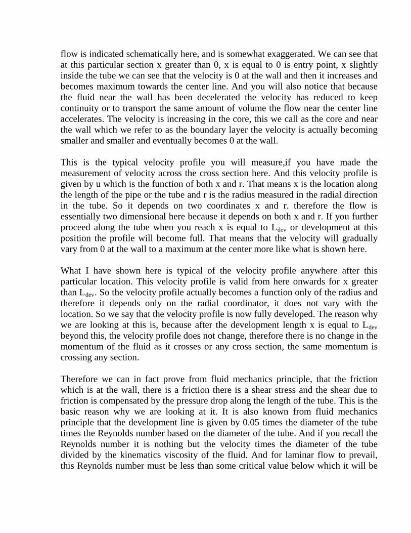
flow is indicated schematically here, and is somewhat exaggerated. We can see that at this particular section x greater than 0, x is equal to 0 is entry point, x slightly inside the tube we can see that the velocity is 0 at the wall and then it increases and becomes maximum towards the center line. And you will also notice that because the fluid near the wall has been decelerated the velocity has reduced to keep continuity or to transport the same amount of volume the flow near the center line accelerates. The velocity is increasing in the core, this we call as the core and near the wall which we refer to as the boundary layer the velocity is actually becoming smaller and smaller and eventually becomes 0 at the wall. This is the typical velocity profile you will measure,if you have made the measurement of velocity across the cross section here. And this velocity profile is given by u which is the function of both x and r. That means x is the location along the length of the pipe or the tube and r is the radius measured in the radial direction in the tube. So it depends on two coordinates x and r. therefore the flow is essentially two dimensional here because it depends on both x and r. If you further proceed along the tube when you reach x is equal to Ldev or development at this position the profile will become full. That means that the velocity will gradually vary from 0 at the wall to a maximum at the center more like what is shown here. What I have shown here is typical of the velocity profile anywhere after this particular location. This velocity profile is valid from here onwards for x greater than Ldev. So the velocity profile actually becomes a function only of the radius and therefore it depends only on the radial coordinator, it does not vary with the location. So we say that the velocity profile is now fully developed. The reason why we are looking at this is, because after the development length x is equal to Ldev beyond this, the velocity profile does not change, therefore there is no change in the momentum of the fluid as it crosses or any cross section, the same momentum is crossing any section. Therefore we can in fact prove from fluid mechanics principle, that the friction which is at the wall, there is a friction there is a shear stress and the shear due to friction is compensated by the pressure drop along the length of the tube. This is the basic reason why we are looking at it. It is also known from fluid mechanics principle that the development line is given by 0.05 times the diameter of the tube times the Reynolds number based on the diameter of the tube. And if you recall the Reynolds number it is nothing but the velocity times the diameter of the tube divided by the kinematics viscosity of the fluid. And for laminar flow to prevail, this Reynolds number must be less than some critical value below which it will be

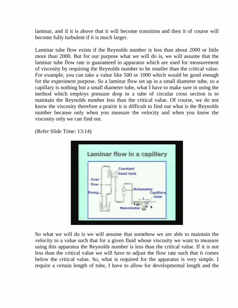
laminar, and if it is above that it will become transition and then it of course will become fully turbulent if it is much larger. Laminar tube flow exists if the Reynolds number is less than about 2000 or little more than 2000. But for our purpose what we will do is, we will assume that the laminar tube flow rate is guaranteed in apparatus which are used for measurement of viscosity by requiring the Reynolds number to be smaller than the critical value. For example, you can take a value like 500 or 1000 which would be good enough for the experiment purpose. So a laminar flow set up in a small diameter tube, so a capillary is nothing but a small diameter tube, what I have to make sure in using the method which employs pressure drop in a tube of circular cross section is to maintain the Reynolds number less than the critical value. Of course, we do not know the viscosity therefore a prairie it is difficult to find out what is the Reynolds number because only when you measure the velocity and when you know the viscosity only we can find out. (Refer Slide Time: 13:14)

So what we will do is we will assume that somehow we are able to maintain the velocity to a value such that for a given fluid whose viscosity we want to measure using this apparatus the Reynolds number is less than the critical value. If it is not less than the critical value we will have to adjust the flow rate such that it comes below the critical value. So, what is required for the apparatus is very simple. I require a certain length of tube, I have to allow for developmental length and the

tube must be longer than the development length plus some length for which I am going to measure the pressure drop. So, I have taken a length equal to L development plus subsequent value L across which I am going to measure the pressure drop which is actually measured using a manometer connected between these two tappings here. One is on the upstream side and one on the downstream side. And in this case I am showing the Rotameter to measure the mass flow rate at the volumetric flow rate and of course, if you know what the volumetric flow rate is and divide by area of cross section of the capillary tube you can get the mean velocity of the flow. And if you remember the Reynolds number is based on that mean velocity which we calculate by taking the volumetric flow rate divided by the area of cross section of the tube. To the left of this Rotameter, I have shown a constant head arrangement because the flow will have to be maintained steady through this tube. That means that the pressure at which it is going to enter this length of tube must be constant, and therefore one way of doing it is to have an overhead tank at a suitable height which can be changed by shifting it up and down as required, and you supply through a pump water or whatever liquid we want to measure the viscosity of that is circulated through this and the excess fluid is going to drain back through an overflow arrangement. That means, I can maintain this level constant. If this level is constant with respect to the level of the tube, there is a given head which is maintained for the flow of the liquid or the fluid through the capillary tube. So the volumetric flow rate is measured here, or if the volumetric flow rate is very small as it happens in most applications of this type, you can actually collect the fluid as it comes out in a graduated jar and measure the volume collected over a certain period of time. A very simple and accurate method is to collect the fluid in a very accurately graduated jar and then measure the volume over a certain time interval which can be measured using a stop watch. And the head h indicated by the manometer gives you the delta p across the tube length L. Actually delta p by L gives you the pressure gradient or the pressure gradient delta p by L. In fact, it can be shown that the pressure gradient is uniform when the flow is fully developed. When the flow is fully developed, and the velocity does not change with respect to the axial location the pressure drop per unit length is the same as the pressure gradient. Let us take a simple example.


Through this example I am going to indicate how one goes about making the measurement of viscosity using flow through a capillarity tube. Example 46: Actually looks at viscosity of water to be measured using laminar flow in a tube of circular cross section. We want to design a suitable set up for this purpose. This will give you some idea on how to go about doing the measurement also. Instead of the usual problem solving, I have taken a design problem, design of this setup, and I am taking water as the fluid or the liquid whose viscosity we want to measure. Here water is the liquid. Let us assume that water is around room temperature. That means that the temperature is something like 25 degree centigrade. So, for design purpose what I can do is, I can take the properties of water roughly at this temperature and then design the setup for that particular condition.


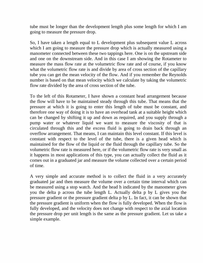
So if you look at the table of properties, basically for the design purpose all we require is the value which is approximately equal to the value which we are going to measure in the experiment. We need not worry about very precise value. We are going to just take the ball park value or the closest to what we want. I can assume that, rho is typically 1000 kg by m cube, this is the density of water and then the viscosity which is the kinematics viscosity nu is about 10 to the power minus 6 m square by sec and it is not multiplied by something which is close to 1 but roughly 10 to the power minus 6 m square by sec. And if you calculate the viscosity mu is nothing but nu into rho and approximately, I will use the symbol like this because it is just the approximate value I am using, this will be 10 to the power minus 3 kg by m.sec which is the unit of viscosity. So now we have a fluid whose viscosity is given and what I have to do is to look at the laminar flow and let us assume that the Reynolds number based on the diameter is roughly 500 and I do not want to exceed this value. If you have very low Reynolds number the pressure drop will become very high. If you go to large Reynolds number then there is a danger that the flow may become turbulent in the experiment. Therefore we have to go for some medium value like this, so I am just taking ReD is equal to 500 as a possible value. And let me also take a diameter of the tube which is the inner diameter of the tube. I will take a suitable value in this case a 3 mm inner diameter tube, 3 mm is not a capillary is fixed of the term but this is a small diameter tube. In fact if you want you can take even a smaller tube. For example, for gases you may be able to take much smaller tube to make the

measurement. So by definition ReD is equal to 500 is the value V the average velocity in this tube multiplied by D by nu and I will substitute the values V into 0.003 (that is 3 mm by 10 to the power minus 6 that is nu as we saw in the previous case). Therefore this gives you a velocity of 500 into 10 to the power minus 6 by 0 0.003, and this is roughly 0.167m by sec or 1.67 cm by sec. Therefore I am talking of a very small velocity of water inside the tube. So you must realize that smaller the velocity of the water, the smaller the Reynolds number in this case. So the idea is to have very small velocity in the tube. In fact I can find out what is the corresponding quantity of flow Q. Q will be nothing velocity times area of cross section of the pipe we will say V into (πD square by 4) and we can substitute so Q is equal to 0.167m by sec which is V multiplied by (π into 0.003) whole square by 4, this will be in m cube by sec and this will come to a value is equal to 1.178 into 10 to the power minus 6 m cube by sec which is same as 1.178 which is roughly 1.2 ml by s. (Refer Slide Time: 27:56)

So, it is just a flow of 1.2 cm cube by sec. It is a very small flow rate. In fact you can immediately see that, I can use an accurate graduated jar which is used very often in the chemical laboratory; all I have to do is to collect this water. For example, if I collect over 100 sec, I will get about 120 cc which will be collected. So I can perform the experiment, for about 100 sec something like 2 minutes I will be able to collect 120 ml which can be very accurately measured. Therefore the volumetric flow rate which I have got here is an accurately measurable quantity in

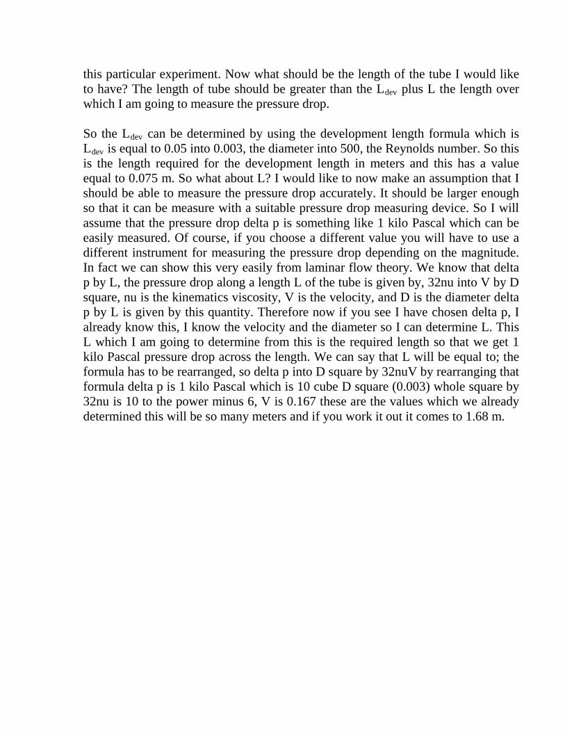
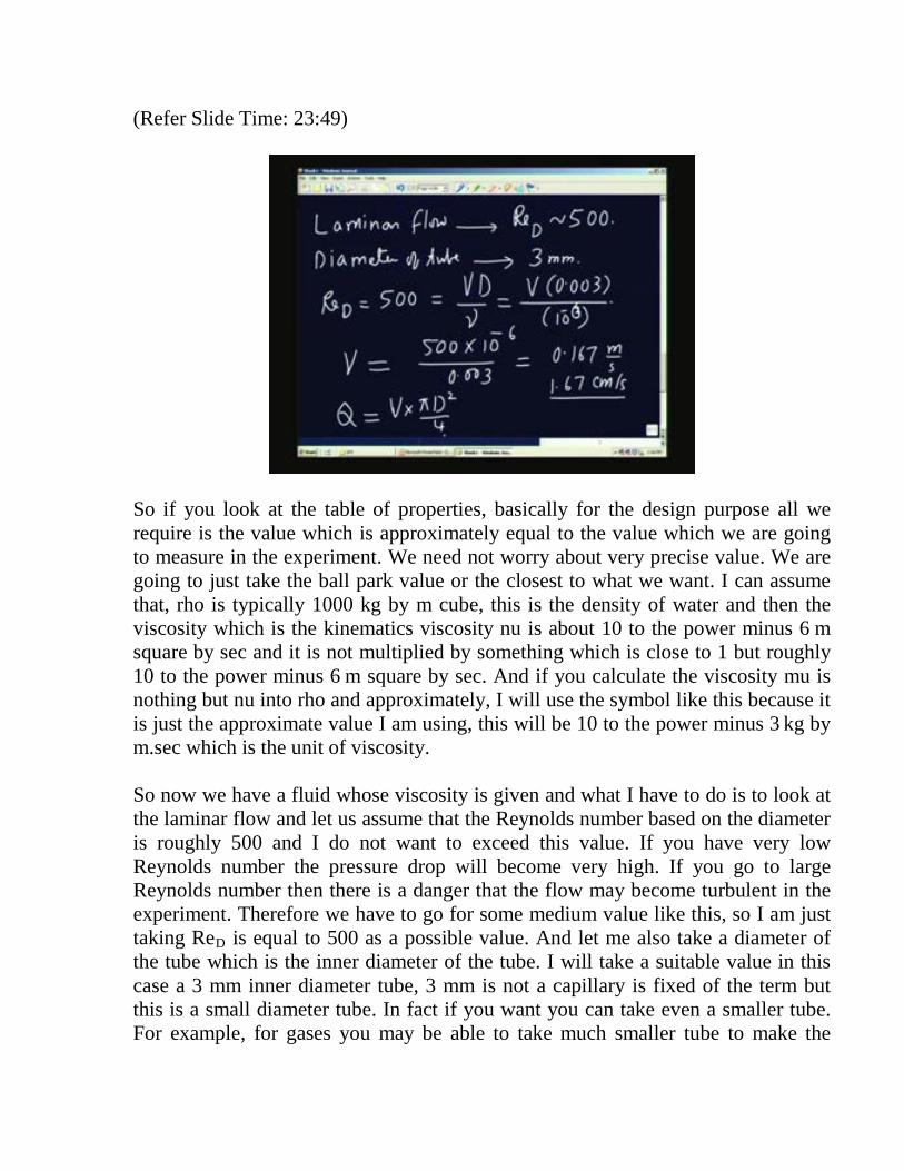
this particular experiment. Now what should be the length of the tube I would like to have? The length of tube should be greater than the Ldev plus L the length over which I am going to measure the pressure drop. So the Ldev can be determined by using the development length formula which is Ldev is equal to 0.05 into 0.003, the diameter into 500, the Reynolds number. So this is the length required for the development length in meters and this has a value equal to 0.075 m. So what about L? I would like to now make an assumption that I should be able to measure the pressure drop accurately. It should be larger enough so that it can be measure with a suitable pressure drop measuring device. So I will assume that the pressure drop delta p is something like 1 kilo Pascal which can be easily measured. Of course, if you choose a different value you will have to use a different instrument for measuring the pressure drop depending on the magnitude. In fact we can show this very easily from laminar flow theory. We know that delta p by L, the pressure drop along a length L of the tube is given by, 32nu into V by D square, nu is the kinematics viscosity, V is the velocity, and D is the diameter delta p by L is given by this quantity. Therefore now if you see I have chosen delta p, I already know this, I know the velocity and the diameter so I can determine L. This L which I am going to determine from this is the required length so that we get 1 kilo Pascal pressure drop across the length. We can say that L will be equal to; the formula has to be rearranged, so delta p into D square by 32nuV by rearranging that formula delta p is 1 kilo Pascal which is 10 cube D square (0.003) whole square by 32nu is 10 to the power minus 6, V is 0.167 these are the values which we already determined this will be so many meters and if you work it out it comes to 1.68 m.


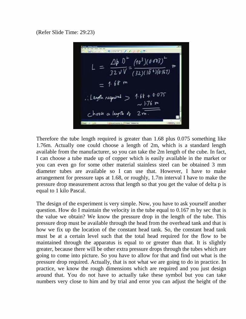
Therefore the tube length required is greater than 1.68 plus 0.075 something like 1.76m. Actually one could choose a length of 2m, which is a standard length available from the manufacturer, so you can take the 2m length of the cube. In fact, I can choose a tube made up of copper which is easily available in the market or you can even go for some other material stainless steel can be obtained 3 mm diameter tubes are available so I can use that. However, I have to make arrangement for pressure taps at 1.68, or roughly, 1.7m interval I have to make the pressure drop measurement across that length so that you get the value of delta p is equal to 1 kilo Pascal. The design of the experiment is very simple. Now, you have to ask yourself another question. How do I maintain the velocity in the tube equal to 0.167 m by sec that is the value we obtain? We know the pressure drop in the length of the tube. This pressure drop must be available through the head from the overhead tank and that is how we fix up the location of the constant head tank. So, the constant head tank must be at a certain level such that the total head required for the flow to be maintained through the apparatus is equal to or greater than that. It is slightly greater, because there will be other extra pressure drops through the tubes which are going to come into picture. So you have to allow for that and find out what is the pressure drop required. Actually, that is not what we are going to do in practice. In practice, we know the rough dimensions which are required and you just design around that. You do not have to actually take these symbol but you can take numbers very close to him and by trial and error you can adjust the height of the

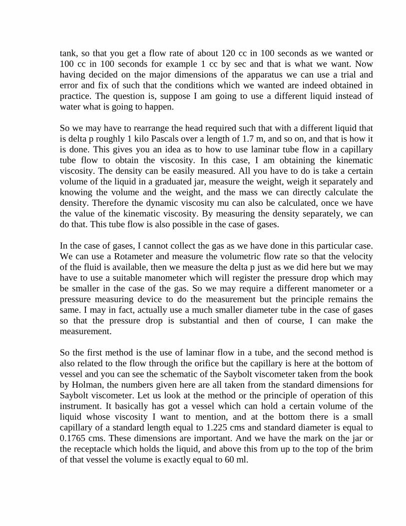
tank, so that you get a flow rate of about 120 cc in 100 seconds as we wanted or 100 cc in 100 seconds for example 1 cc by sec and that is what we want. Now having decided on the major dimensions of the apparatus we can use a trial and error and fix of such that the conditions which we wanted are indeed obtained in practice. The question is, suppose I am going to use a different liquid instead of water what is going to happen. So we may have to rearrange the head required such that with a different liquid that is delta p roughly 1 kilo Pascals over a length of 1.7 m, and so on, and that is how it is done. This gives you an idea as to how to use laminar tube flow in a capillary tube flow to obtain the viscosity. In this case, I am obtaining the kinematic viscosity. The density can be easily measured. All you have to do is take a certain volume of the liquid in a graduated jar, measure the weight, weigh it separately and knowing the volume and the weight, and the mass we can directly calculate the density. Therefore the dynamic viscosity mu can also be calculated, once we have the value of the kinematic viscosity. By measuring the density separately, we can do that. This tube flow is also possible in the case of gases. In the case of gases, I cannot collect the gas as we have done in this particular case. We can use a Rotameter and measure the volumetric flow rate so that the velocity of the fluid is available, then we measure the delta p just as we did here but we may have to use a suitable manometer which will register the pressure drop which may be smaller in the case of the gas. So we may require a different manometer or a pressure measuring device to do the measurement but the principle remains the same. I may in fact, actually use a much smaller diameter tube in the case of gases so that the pressure drop is substantial and then of course, I can make the measurement. So the first method is the use of laminar flow in a tube, and the second method is also related to the flow through the orifice but the capillary is here at the bottom of vessel and you can see the schematic of the Saybolt viscometer taken from the book by Holman, the numbers given here are all taken from the standard dimensions for Saybolt viscometer. Let us look at the method or the principle of operation of this instrument. It basically has got a vessel which can hold a certain volume of the liquid whose viscosity I want to mention, and at the bottom there is a small capillary of a standard length equal to 1.225 cms and standard diameter is equal to 0.1765 cms. These dimensions are important. And we have the mark on the jar or the receptacle which holds the liquid, and above this from up to the top of the brim of that vessel the volume is exactly equal to 60 ml.


So what I am going to do is take 60 ml here, and I want to allow this 60 ml to be drained through this capillary tube, and the time taken is a function of the viscosity of the liquid. And of course in order to maintain the temperature of the entire apparatus as a constant value I can have a constant temperature bath as shown here. If you do not do anything the temperature will be just the atmospheric temperature the room temperature. If you have a constant temperature bath as shown here you can maintain the temperature of any particular value you want so that the viscosity we measure will be a function of temperature because most liquids show a tremendous variation of viscosity with respect to temperature. Therefore if we are interested in measuring the viscosity as the function of temperature we can vary the temperature of the constant temperature bath to suite the measurement required. So you can see that the diameter of the vessel is 2.975 cm these are accurate values. The Saybolt viscometer is manufactured and sold and all these numbers are from such a design. So the entire length from here to here is 12.5 cm. All I have to do here is to fill the inner vessel up to the brim and then start a stopwatch, and then allow this drainage up to this level, and then find out what is the time taken for this operation. The drainage time is related to the viscosity in a somewhat complicated way and the relationship is given actually in the slide here.


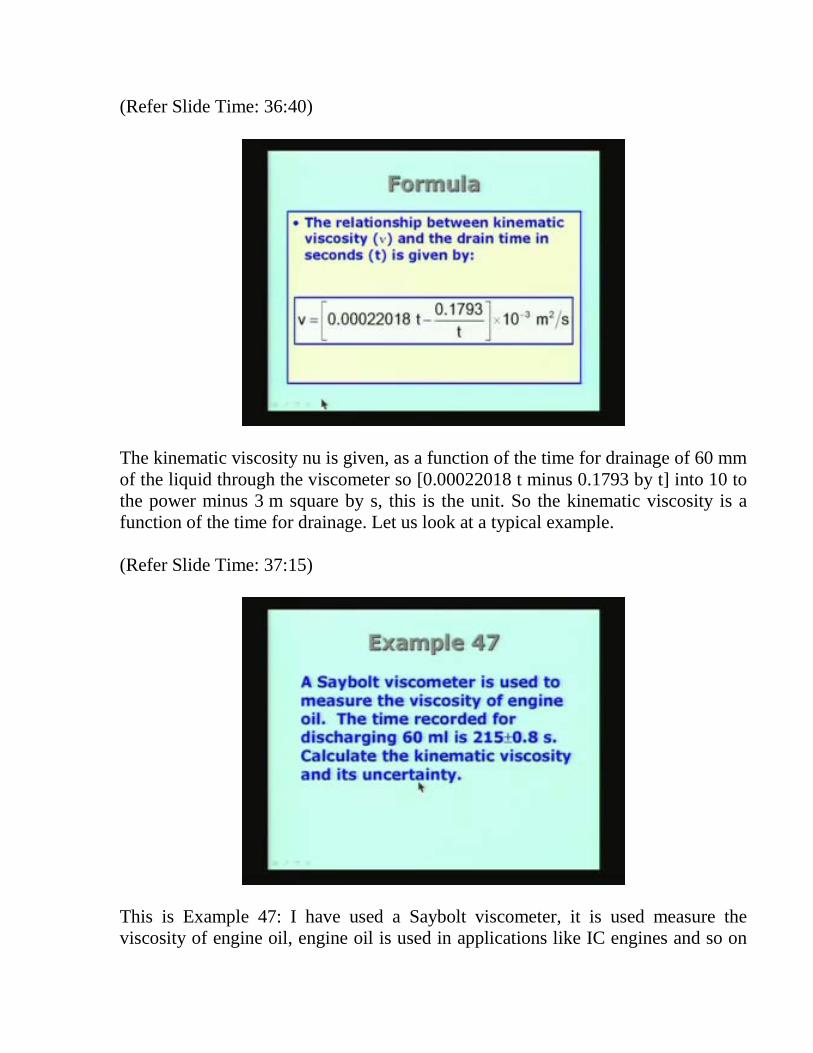
The kinematic viscosity nu is given, as a function of the time for drainage of 60 mm of the liquid through the viscometer so [0.00022018 t minus 0.1793 by t] into 10 to the power minus 3 m square by s, this is the unit. So the kinematic viscosity is a function of the time for drainage. Let us look at a typical example. (Refer Slide Time: 37:15)

This is Example 47: I have used a Saybolt viscometer, it is used measure the viscosity of engine oil, engine oil is used in applications like IC engines and so on

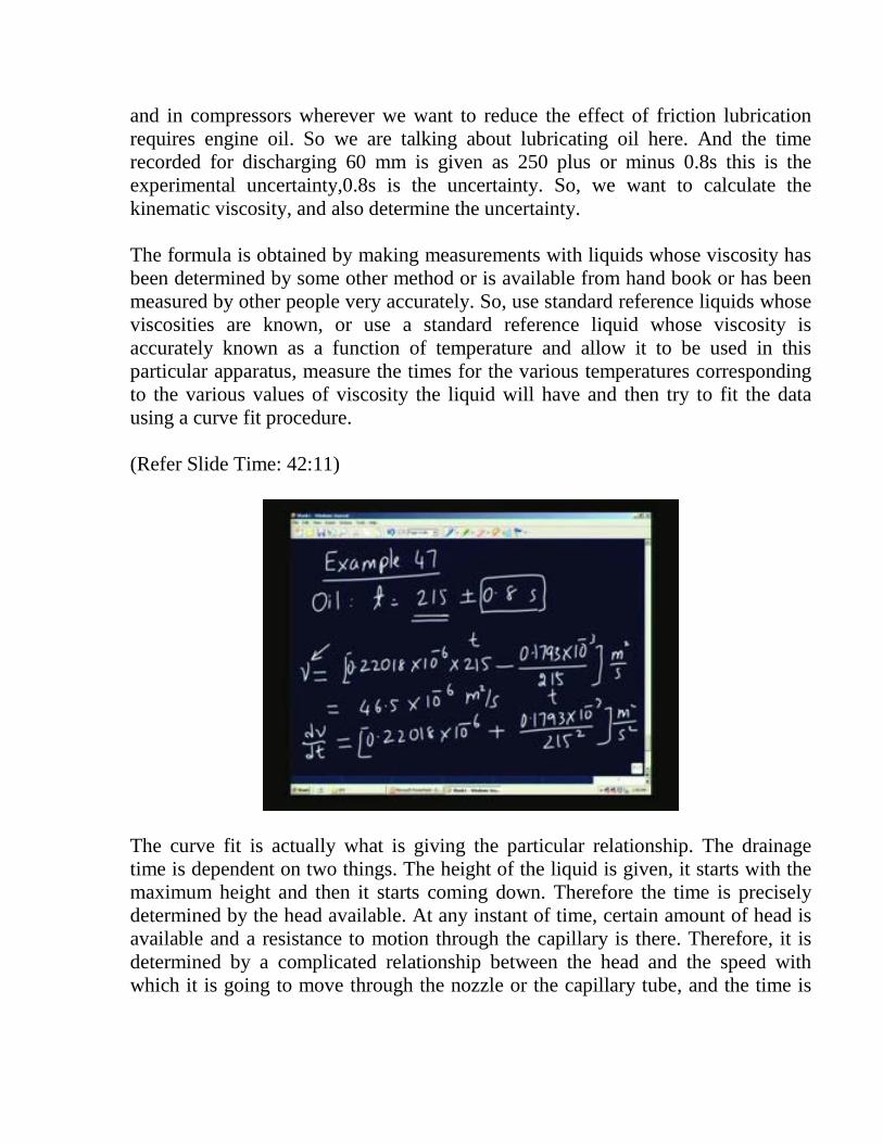
and in compressors wherever we want to reduce the effect of friction lubrication requires engine oil. So we are talking about lubricating oil here. And the time recorded for discharging 60 mm is given as 250 plus or minus 0.8s this is the experimental uncertainty,0.8s is the uncertainty. So, we want to calculate the kinematic viscosity, and also determine the uncertainty. The formula is obtained by making measurements with liquids whose viscosity has been determined by some other method or is available from hand book or has been measured by other people very accurately. So, use standard reference liquids whose viscosities are known, or use a standard reference liquid whose viscosity is accurately known as a function of temperature and allow it to be used in this particular apparatus, measure the times for the various temperatures corresponding to the various values of viscosity the liquid will have and then try to fit the data using a curve fit procedure. (Refer Slide Time: 42:11)

The curve fit is actually what is giving the particular relationship. The drainage time is dependent on two things. The height of the liquid is given, it starts with the maximum height and then it starts coming down. Therefore the time is precisely determined by the head available. At any instant of time, certain amount of head is available and a resistance to motion through the capillary is there. Therefore, it is determined by a complicated relationship between the head and the speed with which it is going to move through the nozzle or the capillary tube, and the time is

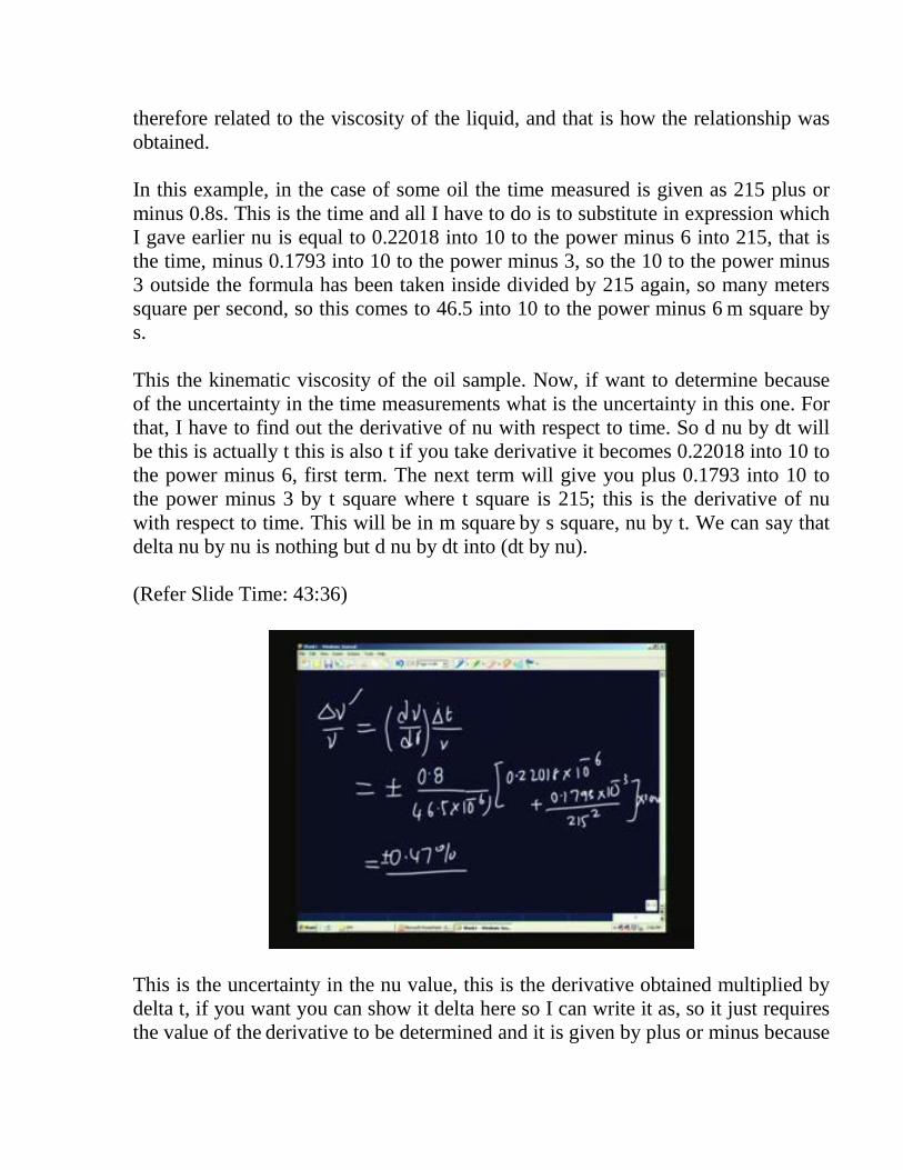
therefore related to the viscosity of the liquid, and that is how the relationship was obtained. In this example, in the case of some oil the time measured is given as 215 plus or minus 0.8s. This is the time and all I have to do is to substitute in expression which I gave earlier nu is equal to 0.22018 into 10 to the power minus 6 into 215, that is the time, minus 0.1793 into 10 to the power minus 3, so the 10 to the power minus 3 outside the formula has been taken inside divided by 215 again, so many meters square per second, so this comes to 46.5 into 10 to the power minus 6 m square by s. This the kinematic viscosity of the oil sample. Now, if want to determine because of the uncertainty in the time measurements what is the uncertainty in this one. For that, I have to find out the derivative of nu with respect to time. So d nu by dt will be this is actually t this is also t if you take derivative it becomes 0.22018 into 10 to the power minus 6, first term. The next term will give you plus 0.1793 into 10 to the power minus 3 by t square where t square is 215; this is the derivative of nu with respect to time. This will be in m square by s square, nu by t. We can say that delta nu by nu is nothing but d nu by dt into (dt by nu). (Refer Slide Time: 43:36)

This is the uncertainty in the nu value, this is the derivative obtained multiplied by delta t, if you want you can show it delta here so I can write it as, so it just requires the value of the derivative to be determined and it is given by plus or minus because

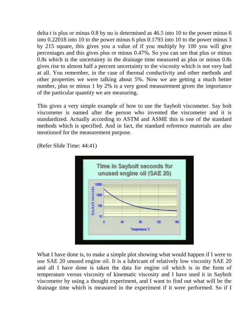
delta t is plus or minus 0.8 by nu is determined as 46.5 into 10 to the power minus 6 into 0.22018 into 10 to the power minus 6 plus 0.1793 into 10 to the power minus 3 by 215 square, this gives you a value of if you multiply by 100 you will give percentages and this gives plus or minus 0.47%. So you can see that plus or minus 0.8s which is the uncertainty in the drainage time measured as plus or minus 0.8s gives rise to almost half a percent uncertainty to the viscosity which is not very bad at all. You remember, in the case of thermal conductivity and other methods and other properties we were talking about 5%. Now we are getting a much better number, plus or minus 1 by 2% is a very good measurement given the importance of the particular quantity we are measuring. This gives a very simple example of how to use the Saybolt viscometer. Say bolt viscometer is named after the person who invented the viscometer and it is standardized. Actually according to ASTM and ASME this is one of the standard methods which is specified. And in fact, the standard reference materials are also mentioned for the measurement purpose. (Refer Slide Time: 44:41)

What I have done is, to make a simple plot showing what would happen if I were to use SAE 20 unused engine oil. It is a lubricant of relatively low viscosity SAE 20 and all I have done is taken the data for engine oil which is in the form of temperature versus viscosity of kinematic viscosity and I have used it in Saybolt viscometer by using a thought experiment, and I want to find out what will be the drainage time which is measured in the experiment if it were performed. So if I

vary the temperature from 0 to 160 degree Celsius the time for drainage, if you see here it is almost 3000s it is going to take about at 0 degree Celsius, this SAE 20 engine oil 60 ml will come out of that Saybolt viscometer in almost one hour. Of course we measure the time very accurately. Suppose you go to some place like 25 or 30 degree which is the room temperature value, you already have about 500 to 600s which is about quarter an hour that is 15 to 20 minutes. And when you go to very high temperature you see that it is a very hot drainage, viscosity is a decreasing function of temperature. As you heat up the oil, the viscosity comes down tremendously and you can see that at this particular position it drains out within about 20 to 30 seconds. The point I want to make here is that, for most liquids whose viscosity we want to measure using Saybolt viscometer the drainage time is measurable and very accurately measurable because it varies from 3000 up to 25 or 30 which is very accurately measurable. In other words, it means that this Saybolt viscometer can be used for large range of values of viscosity of the liquids. The third method I am going to look at is a rotating concentric cylinder apparatus. (Refer Slide Time: 46:56)

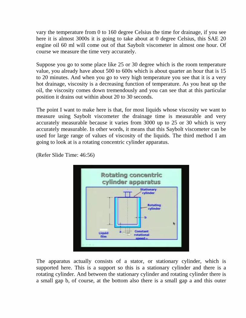
The apparatus actually consists of a stator, or stationary cylinder, which is supported here. This is a support so this is a stationary cylinder and there is a rotating cylinder. And between the stationary cylinder and rotating cylinder there is a small gap b, of course, at the bottom also there is a small gap a and this outer

cylinder is rotated at a constant rotational speed omega. The white patch here is actually the liquid film in between the outer cylinder and the inner cylinder. As I rotate the outer cylinder the film of liquid which is in between the two cylinders is going to undergo a shear, because the velocity of the outer cylinder is radius times omega and the inner cylinder is held fix therefore there is 0 velocity at the edge of the inner cylinder and there is a maximum velocity displaced. And if the gap is narrow, we can actually show that the velocity profile is linear, that means that the velocity varies from 0 to the maximum in a linear fashion. When you have linear velocity profile the shear stress is a constant, because shear stress tau is equal to mu du by dy. If du by dy is equal to a constant because it is linear that means the tau is proportional to mu. So there is a shear stress a constant shear stress which is going to be experienced by the stationery cylinder. Of course, the same shear stress will is also be experienced by the outer cylinder in the opposite direction. Here a small diameter is placed as far as the stationary cylinder is concerned. Suppose, I measure the tortional stress developed or shear stress developed by putting a load cell on the circumference of that, then it is going to measure a stress which is proportional to the torque and that torque is related to the viscosity of the liquid which is going to be in this gap here, as well as the gap here. The length is L, this is b, and this is a, so what we are measuring is the shear stress which is related to the torque and the torque is measured by using the stress which is the strain measured by a load cell, the load cell is going to measure a strain and that strain is proportional to the shear stress which is in turn proportional to the torque, so we can calibrate by suitable means. So the torque is measured related to the viscosity of the liquid which is in the white region shown here. For determining what the torque is, let me try to derive the suitable relationship. What I have essentially is, an inner cylinder and an outer cylinder. This is r1 and this is r2 this is center line here. So the gap b is nothing but, r2 minus r1 the difference between the inner radius of the outer cylinder and the outer radius of the inner cylinder that is r2 minus r1 is the gap b and, of course, at the bottom I have got b the gap equal to a.


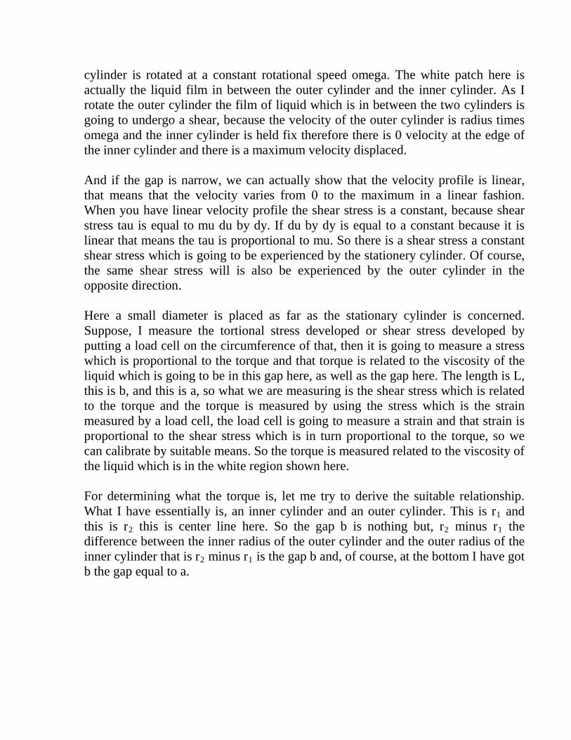
The outer cylinder is rotating, so what is the velocity because of rotation? The velocity will be nothing but r2 times omega, that is the surface speed. And the velocity here is 0, so if I close the gap here this is r1, and this is r2, have the velocity is equal to r2 omega and the velocity is like this, this is 0 and this is equal to r2 omega. Because of this velocity gradient which is of course uniform, there will be a shear stress tau, I am looking at this length is equal to L, and over this length a uniform shear stress is going to be given by mu du by dy which is nothing but, mu into (du by dy) which is nothing but this height divided by this r2 omega by b. Now the shear stress can also be written as the torque divided by the radius arm tau is equal to divided by this will be a force, torque divided by the radius is going to give you a force, and this force divided by the area,is nothing but 2π into r1 into L is the stress. Therefore, the shear stress is nothing but (T1 by r1) by (2πr1L) is equal to mu into du by dy is equal to mu into r2 omega by b. So this gives you a torque is equal to T1, from here I can work out a torque is equal to T1 and it can be written as, torque,T1 is equal to 2π into mu r1 square r2 into L omega by b. We will call this is as expression 1. Now let us look at the torque due to the film which is at the bottom of the cylinder. So if draw the bottom of the cylinder this is the axis and there is a gap of a. And at any location at radius is equal to r this part is moving, this part is stationary, this is moving with velocity is equal to omega times r and this is 0 velocity.


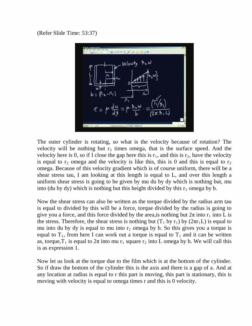
So, if I look at the velocity field there, I can show it like this, this is 0, this is omega r and the velocity will show a linear variation like this. Therefore, corresponding to this, we have a shear stress which is a function of r which is given by, this r omega is the velocity divided by the gap which is, a multiplied by mu, mu r omega by a. And this shear stress we can assume that we can take a small length over which this is the value of shear stress delta r we can say or dr, so what is the area over which it occurs? Area as the function of r is given by 2π r dr. Therefore this is like a shear force or a force is equal to tau into a, it will give you (2π into omega into mu by a) into r2 dr and this is going to give rise to a torque, so we will call it the elemental torque. You have to multiply by another factor of r, so 2π omega mu by a into r

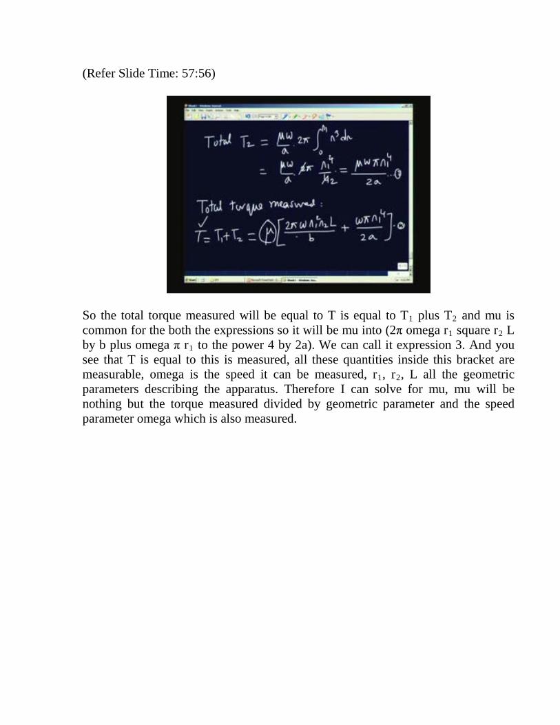
cube dr. Now what I have to do is, to calculate the total torque due to these elemental torque therefore 2π omega mu by a into r cube dr. Here is expression 1; 2 mu π r1 square r2 L by b2.


So the total torque measured will be equal to T is equal to T1 plus T2 and mu is common for the both the expressions so it will be mu into (2π omega r1 square r2 L by b plus omega π r1 to the power 4 by 2a). We can call it expression 3. And you see that T is equal to this is measured, all these quantities inside this bracket are measurable, omega is the speed it can be measured, r1, r2, L all the geometric parameters describing the apparatus. Therefore I can solve for mu, mu will be nothing but the torque measured divided by geometric parameter and the speed parameter omega which is also measured.


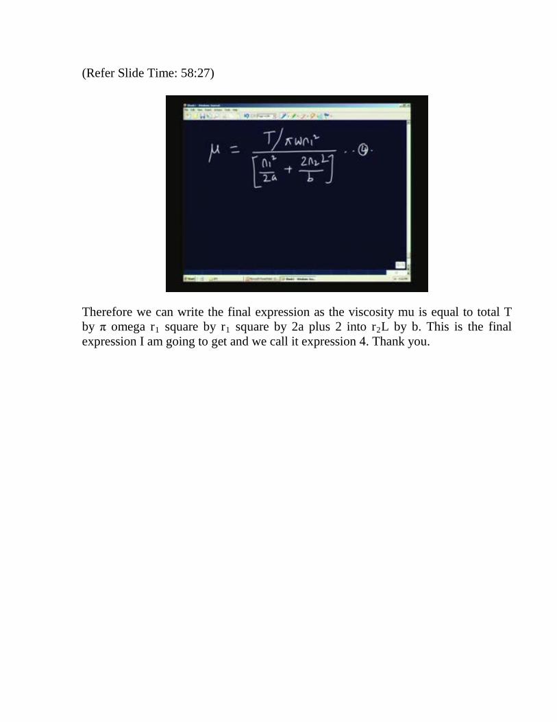
Therefore we can write the final expression as the viscosity mu is equal to total T by π omega r1 square by r1 square by 2a plus 2 into r2L by b. This is the final expression I am going to get and we call it expression 4. Thank you.

mechanical measurements and metrology prof. s. p...

Documents