Mechanical Measurements and Metrology Prof. S. P. Venkateshan

Department of Mechanical Engineering Indian Institute of Technology, Madras

Module - 1 Lecture - 2

Errors in Measurements

So this will be our second lecture in the series on Mechanical Measurements. We would like to just recapitulate some of the things we did in the first lecture. (Refer Slide Time 1:10)

It was mostly introductory in nature; it introduced the topics, which we are going to recover in module 1 and then we started off with a description of the reasons one wants to do measurements. It was followed by the basic idea of measurements and also it described what to expect in a measurement. Usually a measurement is accommodated by some errors; we identified two types of errors: the systematic as well as random errors and the systematic errors give rise to what is called bias and the random errors give rise to random fluctuations and they are statistical in nature. So the whole idea was to look at these two different types of errors and see what we can do, how we can analyze the data taking into account that there may be bias and also random errors. The bias can be eliminated or reduced by suitable

manipulations; however, the random errors are going to be present, whatever may be the care we have taken in making the measurements and we require looking at these random errors by what is called statistical analysis. So what we are going to do in the present lecture is to continue that topic and we are going to look at the errors, their distribution, how to analyze them statistically and also how to characterize these and how to obtain the best possible measurement from a given set of data. We will describe these in more detail as we go along I will also take one or two examples to highlight what we are doing. So to just spell out, we are going to look at the error distributions with some typical example and I will also follow it with a general example. Then I will get into the statistical analysis of measurement errors. So we are going to ask ourselves the question, what is the best estimate for a measured quantity? You may now notice that I am using the term estimate; so this particular term is going to be used very often. We never say that we have a correct or right value for the measured quantity. We always call it an estimate because the measurement gives only an estimate for the measured value or measured quantity. So the idea is to find out what is the best estimate from the measurements we have performed. It may or may not be exactly equal to what is expected or what the true value of the measured quantity is. If you are able to eliminate or reduce the bias, which may be there in the measured values by a suitable method, then we will be able to estimate the errors in the measured quantity. These errors are due to the random fluctuations and therefore the estimate and the estimation of the errors accompanying the measurement are what we are going to look at. We will follow it up with a typical example, which will be highlighting whatever we have discussed by then.

(Refer Slide Time: 4:30)

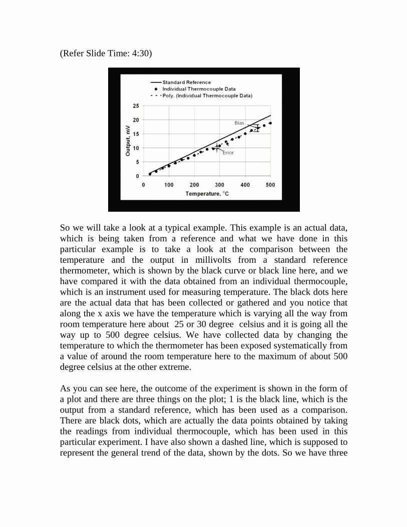
So we will take a look at a typical example. This example is an actual data, which is being taken from a reference and what we have done in this particular example is to take a look at the comparison between the temperature and the output in millivolts from a standard reference thermometer, which is shown by the black curve or black line here, and we have compared it with the data obtained from an individual thermocouple, which is an instrument used for measuring temperature. The black dots here are the actual data that has been collected or gathered and you notice that along the x axis we have the temperature which is varying all the way from room temperature here about 25 or 30 degree celsius and it is going all the way up to 500 degree celsius. We have collected data by changing the temperature to which the thermometer has been exposed systematically from a value of around the room temperature here to the maximum of about 500 degree celsius at the other extreme. As you can see here, the outcome of the experiment is shown in the form of a plot and there are three things on the plot; 1 is the black line, which is the output from a standard reference, which has been used as a comparison. There are black dots, which are actually the data points obtained by taking the readings from individual thermocouple, which has been used in this particular experiment. I have also shown a dashed line, which is supposed to represent the general trend of the data, shown by the dots. So we have three

things here: the black line representing the reference, which is assumed to represent, in some sense, the truth. Secondly, we have the dots, which represent the actual data gathered from the individual experiment and then we have the dashed line, which is supposed to represent the trend of the data, the general variation of the data. What we notice from this figure is that there is a systematic difference between the black line and the dashed line, so between the black line and dashed line, the dashed line is supposed to represent the general trend of the data and of course, we will come later to the question of how to get this trend and what is the method we are going to use. These will be discussed later on. But right now, let us assume that we have somehow got a trend and then there is a systematic difference between the black line and the dashed line. This is the bias and of course, in this particular example, the bias is a function of temperature. At 300, for example, the bias is this much, and at 400 it will go here. You will see that the bias has already changed and if you go to 500 further there is a change in the bias. Therefore, bias in general can be a function of the variable on the x axis, which usually is going to be the one which we are going to control. The output, on the other hand, which is shown on the y axis, is the one which we are going to measure by keeping the control variable at a constant value as shown in the x axis. You will notice another thing that the black dots are not lying on the trend line at all, so the black dots are distributed around the trend line and possibly more or less evenly distributed on the two sides of the trend line. That means the difference between the black dots and the value represented by the dashed line can be either positive or negative; it can sometimes be small or sometimes large, as you can see here. So the error between the trend line and the black dots is what I call as the error and this error is due to random fluctuations. Just to explain it a little further, suppose I have to do an experiment at 300 degrees and if I repeat the experiment again and again, this black dot is only 1 such value that I have got. I will get a set of values at this particular value of our 300, which will vary. It will not give the same value as shown by this black dot. It will keep on fluctuating, keep on varying. Each experiment you repeat, you will get some variation and that is one kind of variation.

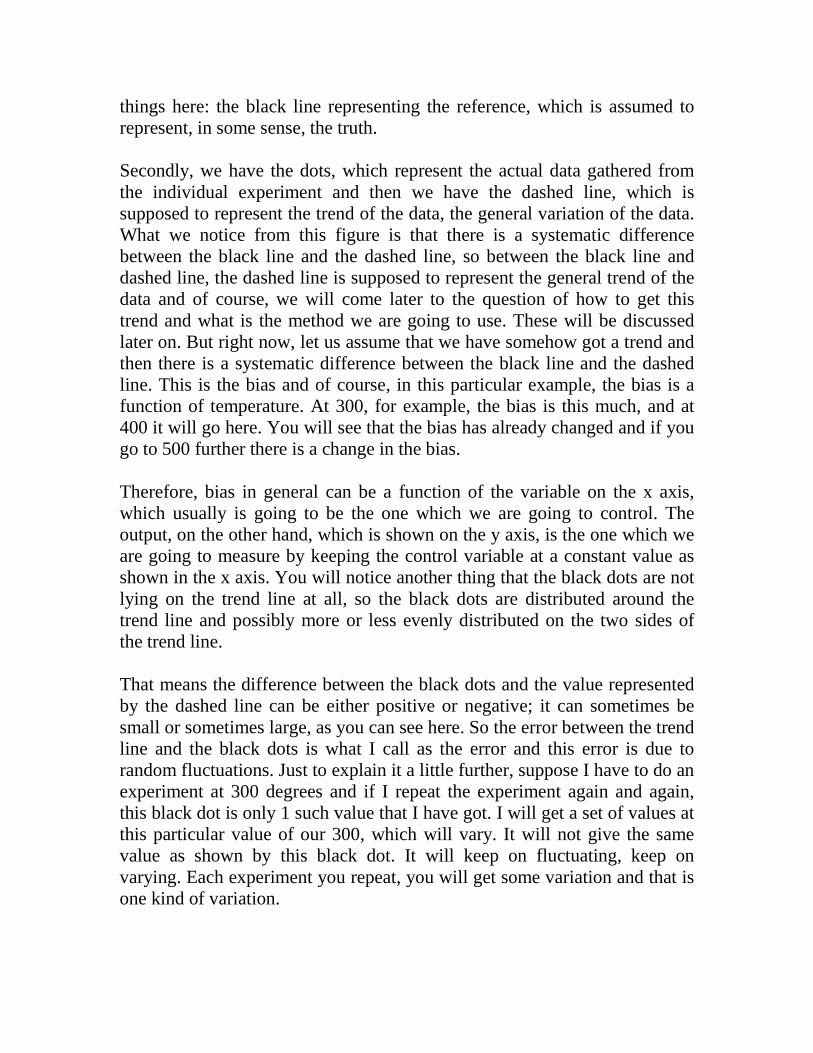
The second kind of variation is when you change the temperature, at each temperature, you get a fluctuation. So if we assume that these two fluctuations are going to be related to each other, that means they are going to come out and they are basically due to same randomness in the experiment, which we are carrying out. The two are going to have roughly the same statistics. This is going to play a very important role when we discuss more fully the way we are going to construct the trend line in this particular case. So this is basically what you are going to expect from any measurement and in this case I have taken a specific measurement of comparison between a thermocouple, which is used to measure the temperature and a standard reference, which is also used to measure the same temperature. The assumption being that at any instant of time, the two, the standard references as well as the individual thermocouple, are exposed to the same temperature on the outside. Now with this background, let us look at the next slide, which indicates a general example. So the next example, which is a general one, is slightly different in the sense that the relationship is not any close to a linear type of relationship which we saw in the case of the temperature measurement. In this case, the trend could be a curve instead of being more or less a straight line as in the previous case. And therefore it is a more general case. (Refer Slide Time 10:55)

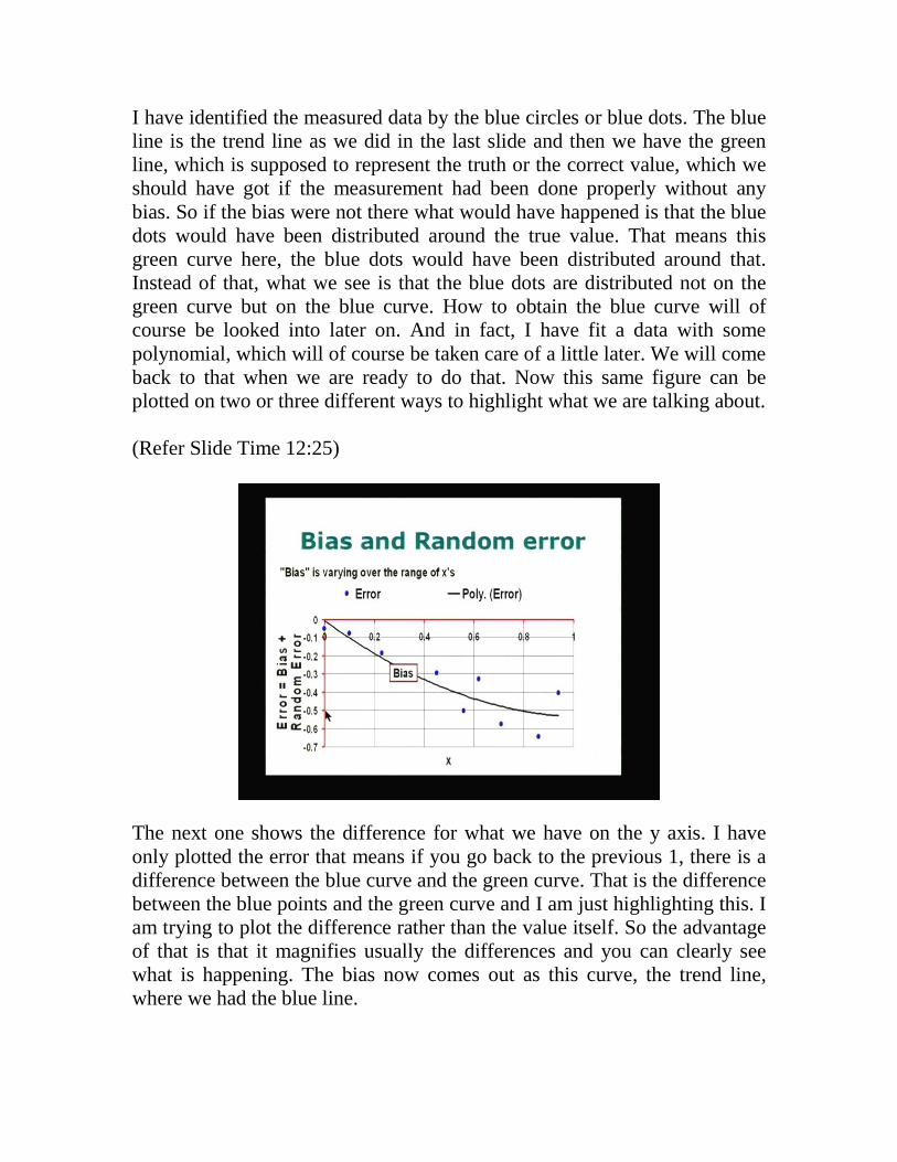
I have identified the measured data by the blue circles or blue dots. The blue line is the trend line as we did in the last slide and then we have the green line, which is supposed to represent the truth or the correct value, which we should have got if the measurement had been done properly without any bias. So if the bias were not there what would have happened is that the blue dots would have been distributed around the true value. That means this green curve here, the blue dots would have been distributed around that. Instead of that, what we see is that the blue dots are distributed not on the green curve but on the blue curve. How to obtain the blue curve will of course be looked into later on. And in fact, I have fit a data with some polynomial, which will of course be taken care of a little later. We will come back to that when we are ready to do that. Now this same figure can be plotted on two or three different ways to highlight what we are talking about. (Refer Slide Time 12:25)

The next one shows the difference for what we have on the y axis. I have only plotted the error that means if you go back to the previous 1, there is a difference between the blue curve and the green curve. That is the difference between the blue points and the green curve and I am just highlighting this. I am trying to plot the difference rather than the value itself. So the advantage of that is that it magnifies usually the differences and you can clearly see what is happening. The bias now comes out as this curve, the trend line, where we had the blue line.

The difference between the blue line and the green line or the distance between the two is of course varying with respect to x and it comes out as a curve like this and the bias is clearly seen here. You also see that the blue dots are distributed around the bias in a systematic fashion like this, in some kind of a random fashion, but the difference here is smaller; here it is bigger. So the bias, the difference seems to be little larger here, of course, it should be due to only accidental reason. So let us look at another way of making a plot. (Refer Slide Time 13:45)

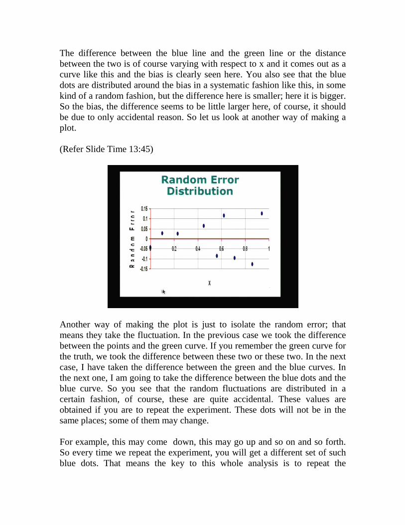
Another way of making the plot is just to isolate the random error; that means they take the fluctuation. In the previous case we took the difference between the points and the green curve. If you remember the green curve for the truth, we took the difference between these two or these two. In the next case, I have taken the difference between the green and the blue curves. In the next one, I am going to take the difference between the blue dots and the blue curve. So you see that the random fluctuations are distributed in a certain fashion, of course, these are quite accidental. These values are obtained if you are to repeat the experiment. These dots will not be in the same places; some of them may change. For example, this may come down, this may go up and so on and so forth. So every time we repeat the experiment, you will get a different set of such blue dots. That means the key to this whole analysis is to repeat the

measurement again and again, and each time you repeat the measurement you are going to get these blue dots distributed not the same way. They are going to keep on changing, but these blue dots will have some statistical properties, which is what we would like to look at. For example, if you go back to the slide, you see that if I were to project all these blue dots on to the y axis if I were to project this like this I go I take a straight line here and put it here, another here and here and so on, you will see that the dots will be distributed along this line in a certain fashion. So we would like to know the distribution of these blue dots on the y axis. Can we characterize this distribution mathematically and if so what are the characteristics of that particular curve? These are going to be important if you want to understand the errors and their behavior and their characteristic. So with this view, let us see what one may expect. It is not that every time we are going to expect this. But if you were to do the experiment again and again and if the method of measurements is not different each time, every time we repeat the experiment we do it with equal care then we can expect, as you saw here in previous graph, these dots are going to be distributed in some random fashion. They will form a certain distribution. What is the characteristic of distribution? The positive errors and the random errors we are talking about, the positive values and negative values are equally likely. Positive large values and negative large values are equally likely. That means the distribution must show some kind of symmetry with respect to the 0 line here. So the random error shows some kind of symmetry with respect to the x axis or the 0 error axis and these are going to have a distribution that is symmetrical. And the 1 symmetrical distribution we are very familiar with is called the normal distribution and I have given the expression for the normal distribution in this slide.

(Refer Slide Time 17:00)

(Refer Slide Time: 17: 20)

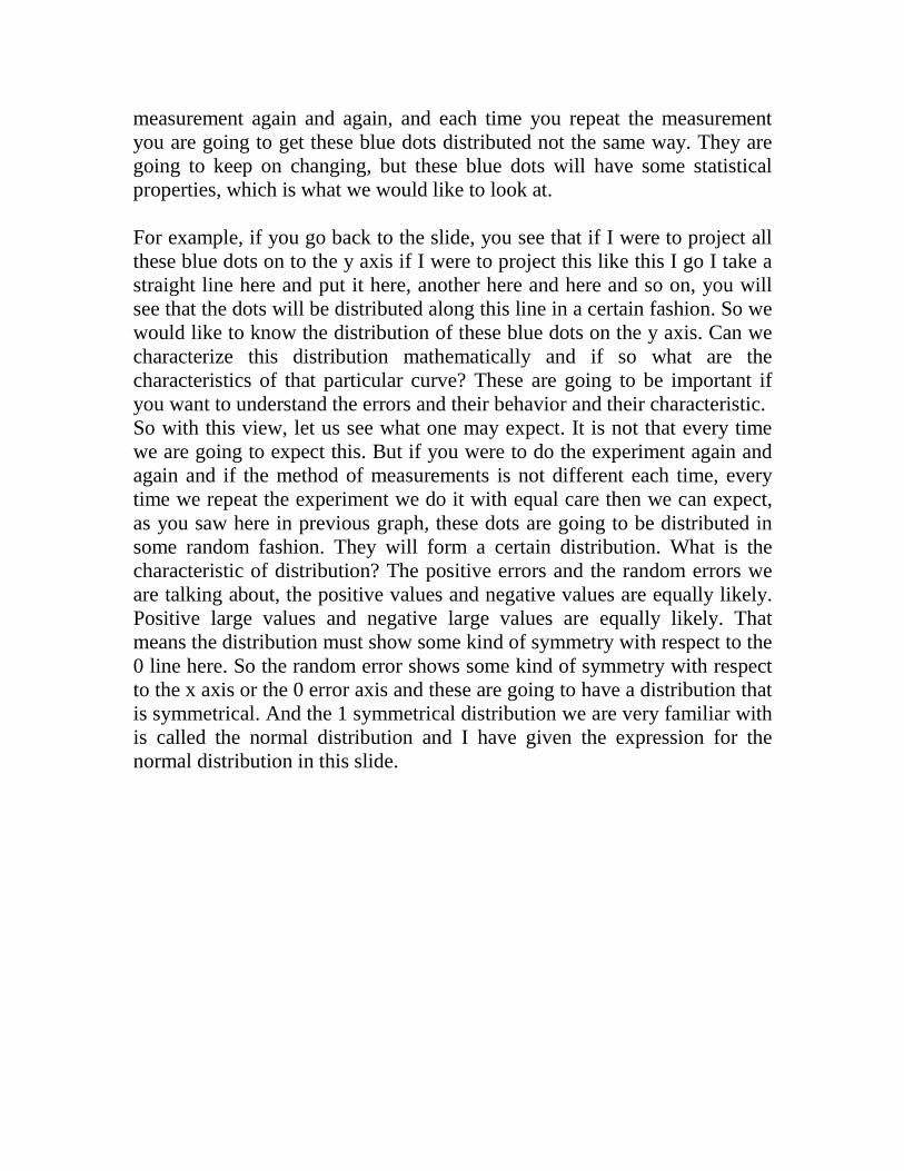
So, random errors may be distributed as a normal distribution. If I indicate the mean of the values as mu, and go back to the previous slide where the mean is 0, in this case .Of course mean could be some value. I can subtract it out and make it equal to 0 just for convenience. If sigma is the standard deviation with respect to the mean we will define sigma more fully and we will find out how to determine sigma from measured values and so on. So the mean and the standard deviation represent mu and sigma, a probability

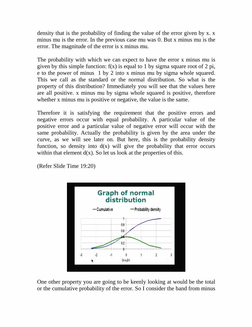
density that is the probability of finding the value of the error given by x. x minus mu is the error. In the previous case mu was 0. But x minus mu is the error. The magnitude of the error is x minus mu. The probability with which we can expect to have the error x minus mu is given by this simple function: f(x) is equal to 1 by sigma square root of 2 pi, e to the power of minus 1 by 2 into x minus mu by sigma whole squared. This we call as the standard or the normal distribution. So what is the property of this distribution? Immediately you will see that the values here are all positive. x minus mu by sigma whole squared is positive, therefore whether x minus mu is positive or negative, the value is the same. Therefore it is satisfying the requirement that the positive errors and negative errors occur with equal probability. A particular value of the positive error and a particular value of negative error will occur with the same probability. Actually the probability is given by the area under the curve, as we will see later on. But here, this is the probability density function, so density into d(x) will give the probability that error occurs within that element d(x). So let us look at the properties of this. (Refer Slide Time 19:20)

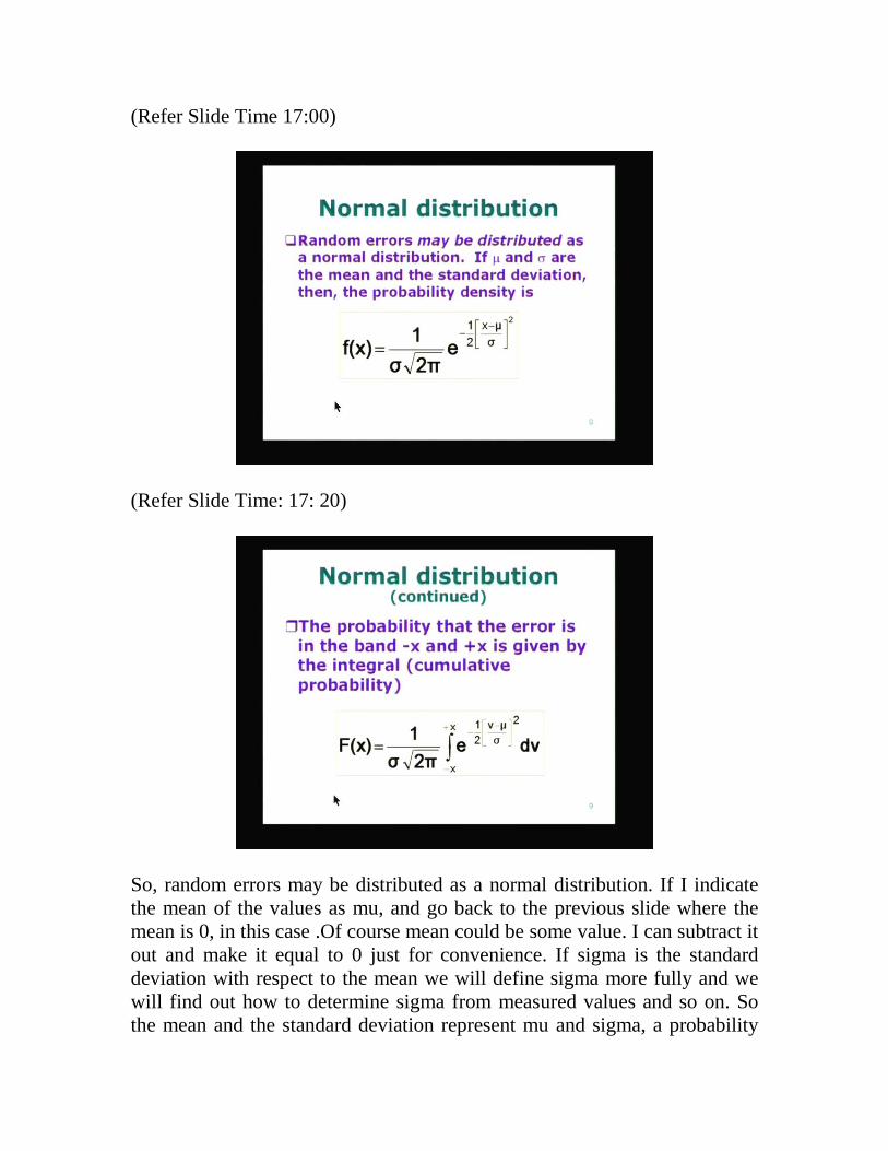
One other property you are going to be keenly looking at would be the total or the cumulative probability of the error. So I consider the band from minus

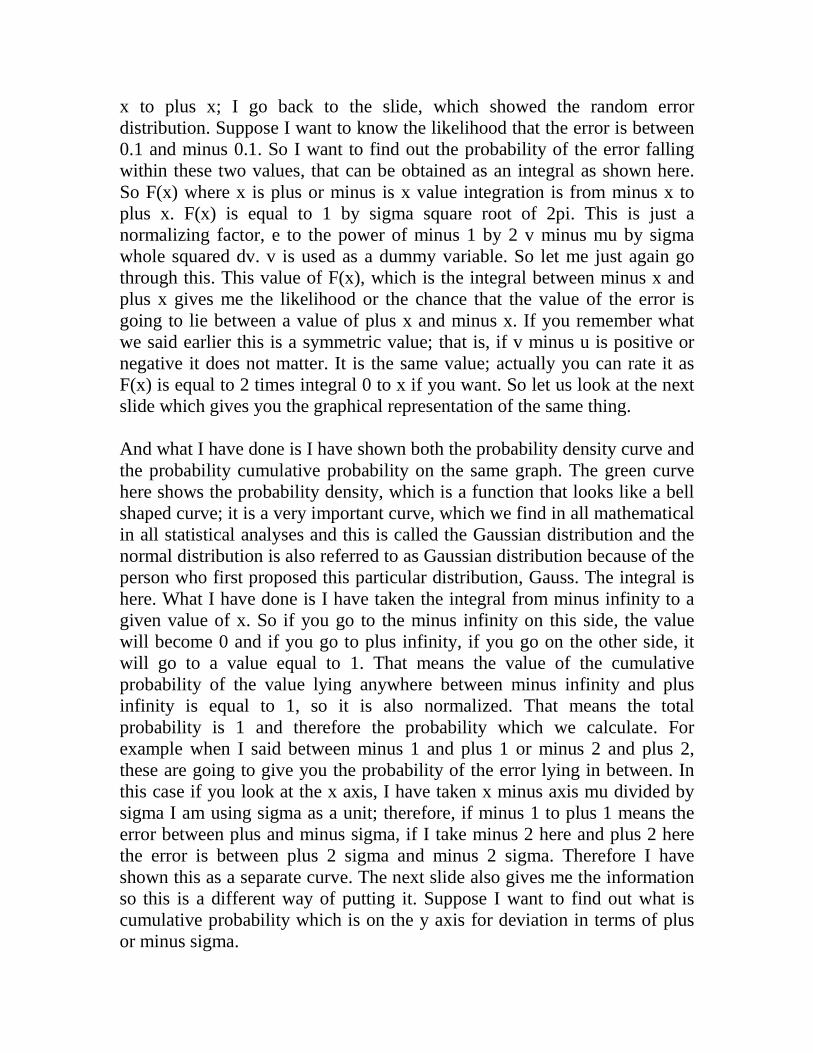
x to plus x; I go back to the slide, which showed the random error distribution. Suppose I want to know the likelihood that the error is between 0.1 and minus 0.1. So I want to find out the probability of the error falling within these two values, that can be obtained as an integral as shown here. So F(x) where x is plus or minus is x value integration is from minus x to plus x. F(x) is equal to 1 by sigma square root of 2pi. This is just a normalizing factor, e to the power of minus 1 by 2 v minus mu by sigma whole squared dv. v is used as a dummy variable. So let me just again go through this. This value of F(x), which is the integral between minus x and plus x gives me the likelihood or the chance that the value of the error is going to lie between a value of plus x and minus x. If you remember what we said earlier this is a symmetric value; that is, if v minus u is positive or negative it does not matter. It is the same value; actually you can rate it as F(x) is equal to 2 times integral 0 to x if you want. So let us look at the next slide which gives you the graphical representation of the same thing. And what I have done is I have shown both the probability density curve and the probability cumulative probability on the same graph. The green curve here shows the probability density, which is a function that looks like a bell shaped curve; it is a very important curve, which we find in all mathematical in all statistical analyses and this is called the Gaussian distribution and the normal distribution is also referred to as Gaussian distribution because of the person who first proposed this particular distribution, Gauss. The integral is here. What I have done is I have taken the integral from minus infinity to a given value of x. So if you go to the minus infinity on this side, the value will become 0 and if you go to plus infinity, if you go on the other side, it will go to a value equal to 1. That means the value of the cumulative probability of the value lying anywhere between minus infinity and plus infinity is equal to 1, so it is also normalized. That means the total probability is 1 and therefore the probability which we calculate. For example when I said between minus 1 and plus 1 or minus 2 and plus 2, these are going to give you the probability of the error lying in between. In this case if you look at the x axis, I have taken x minus axis mu divided by sigma I am using sigma as a unit; therefore, if minus 1 to plus 1 means the error between plus and minus sigma, if I take minus 2 here and plus 2 here the error is between plus 2 sigma and minus 2 sigma. Therefore I have shown this as a separate curve. The next slide also gives me the information so this is a different way of putting it. Suppose I want to find out what is cumulative probability which is on the y axis for deviation in terms of plus or minus sigma.

(Refer Slide Time 22:53)

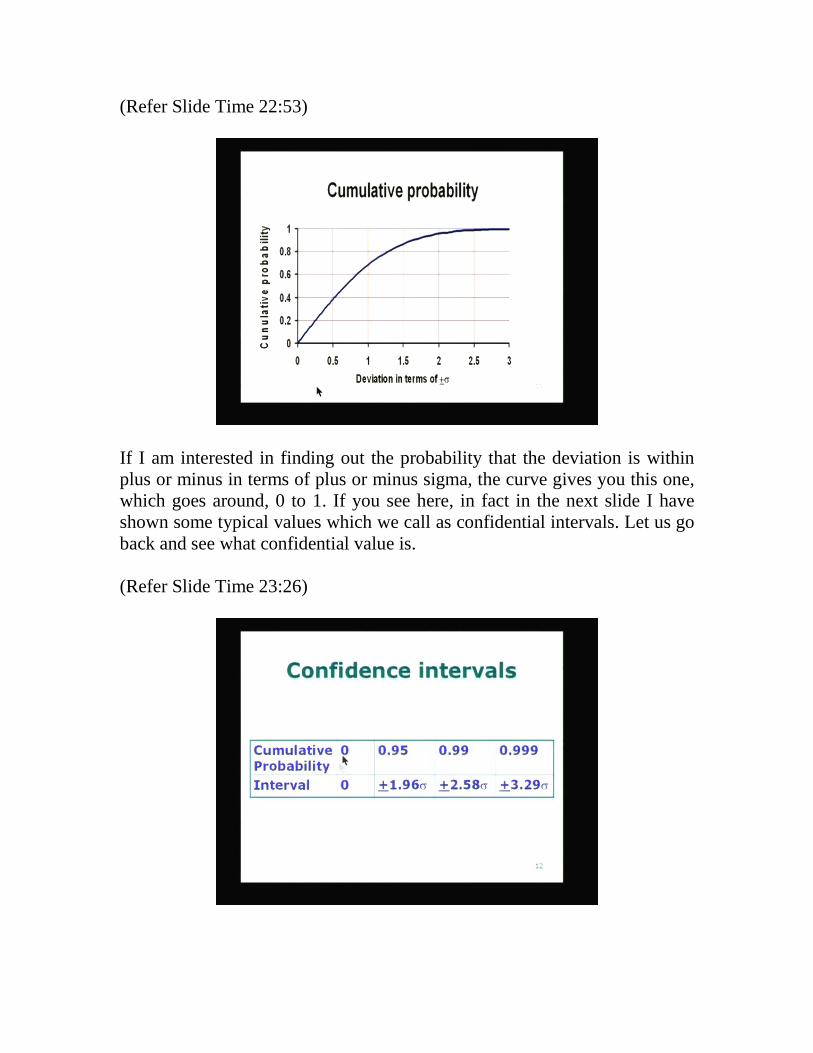
If I am interested in finding out the probability that the deviation is within plus or minus in terms of plus or minus sigma, the curve gives you this one, which goes around, 0 to 1. If you see here, in fact in the next slide I have shown some typical values which we call as confidential intervals. Let us go back and see what confidential value is. (Refer Slide Time 23:26)

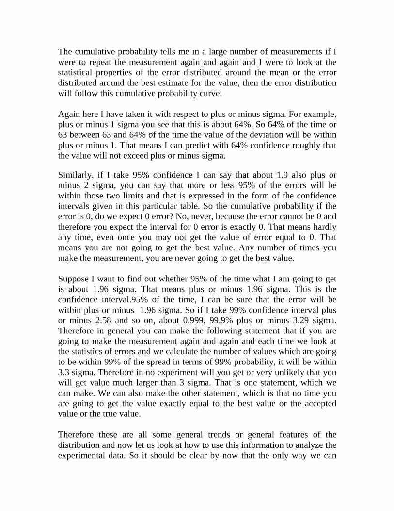
The cumulative probability tells me in a large number of measurements if I were to repeat the measurement again and again and I were to look at the statistical properties of the error distributed around the mean or the error distributed around the best estimate for the value, then the error distribution will follow this cumulative probability curve. Again here I have taken it with respect to plus or minus sigma. For example, plus or minus 1 sigma you see that this is about 64%. So 64% of the time or 63 between 63 and 64% of the time the value of the deviation will be within plus or minus 1. That means I can predict with 64% confidence roughly that the value will not exceed plus or minus sigma. Similarly, if I take 95% confidence I can say that about 1.9 also plus or minus 2 sigma, you can say that more or less 95% of the errors will be within those two limits and that is expressed in the form of the confidence intervals given in this particular table. So the cumulative probability if the error is 0, do we expect 0 error? No, never, because the error cannot be 0 and therefore you expect the interval for 0 error is exactly 0. That means hardly any time, even once you may not get the value of error equal to 0. That means you are not going to get the best value. Any number of times you make the measurement, you are never going to get the best value. Suppose I want to find out whether 95% of the time what I am going to get is about 1.96 sigma. That means plus or minus 1.96 sigma. This is the confidence interval.95% of the time, I can be sure that the error will be within plus or minus 1.96 sigma. So if I take 99% confidence interval plus or minus 2.58 and so on, about 0.999, 99.9% plus or minus 3.29 sigma. Therefore in general you can make the following statement that if you are going to make the measurement again and again and each time we look at the statistics of errors and we calculate the number of values which are going to be within 99% of the spread in terms of 99% probability, it will be within 3.3 sigma. Therefore in no experiment will you get or very unlikely that you will get value much larger than 3 sigma. That is one statement, which we can make. We can also make the other statement, which is that no time you are going to get the value exactly equal to the best value or the accepted value or the true value. Therefore these are all some general trends or general features of the distribution and now let us look at how to use this information to analyze the experimental data. So it should be clear by now that the only way we can

understand the nature of the errors is to repeat the experiment any number of times, whatever number of times it is possible. If it is very expensive, of course, the experiment may be done only once or twice and therefore we are limited by the amount of time and effort we can spend. But in some simple experiments, we can do it any number of times within reasonable limit and therefore that can be done at least notionally. We can assume that any experiment is possible to repeat any number of times so that the nature of errors can be obtained by looking at the sample of data. We call it sample because we can repeat the experiment and get another sample, another set of data and so on and so forth. So this is called sampling and unfortunately we don’t have too much time to go into the details of statistical analysis, to the depth which is desired may be at a higher level. But here we will just look at the some of the things we can achieve by not doing a study in great depth. We will try to find out what is required for us by looking at simple things. (Refer Slide Time 27:54)

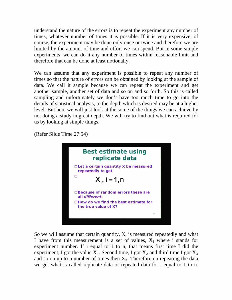
So we will assume that certain quantity, X, is measured repeatedly and what I have from this measurement is a set of values, Xi where i stands for experiment number. If i equal to 1 to n, that means first time I did the experiment, I got the value X1. Second time, I got X2 and third time I got X3 and so on up to n number of times then Xn. Therefore on repeating the data we get what is called replicate data or repeated data for i equal to 1 to n.

What we will notice once we get data like this is that it’s because of random errors that all these are going to be different. Of course many of them may be close to each other, and if we round off for example, some of them actually will look like alike there. But if we use the sufficient number of digits on the decimal points and so on you can actually see the difference. Of course in any experiment we use a certain number of decimal points to represent the number and therefore within that some may appear to be same but in general these are different values of the same measured quantity obtained by repeating the experiment again and again assuming that the reputation is possible and not very expensive. So the question we are going to ask is, how do we find the best estimate for the true value of X? Why am I using the term estimate because I am not going to get the true value; I am very clear about it. What I can do is to estimate the value, which may be expected to be close to the true value. Whatever may be the true value, we don’t know. So we are happy; if we can get estimate, which is closest to the true value and I may or may not know how close it is. It depends on the particular experiment and so on. So let us look at the principle involved behind this particular estimation and that requires a little bit of understanding of the nature of the error. We have already said that the errors are distributed in a normal fashion and therefore if I go back to the experiment, which was given in the earlier slide, I have varied X. That doesn’t matter, if you work to just take the values and project it on the y axis. I said earlier that you are going to get a certain density of these and these points are going to lie on this. If you divide this 0 to 0.15 for example, if I divide into 3 ranges let us see 0 to 0.05, 0.05 to 0.1, 0.1 to 0.15 similarly on the negative side also I can do the same thing. So two points are lying in between 0 to 0.05 and 1 point lying between 0.05 to 0.1 and 2 of them are lying between 0.1 and 0.15. Of course if I have to repeat the experiment, these values may be different. So what I am going to look at now is I am going to ask myself the question, why is it that I have got these two values between 0.0 and 0.05? I got these values because it was a probable outcome of the experiment. The experiment was such that these values had to occur and if it were to occur, these errors have to occur according to the normal distribution. What I can do is I can use the normal distribution, which is shown here, and what I have done is, I have written it in a slightly different form here.

(Refer Slide Time 32:09)

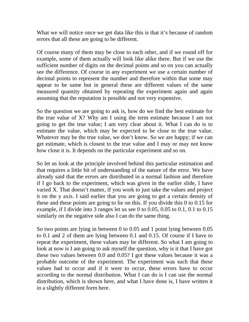
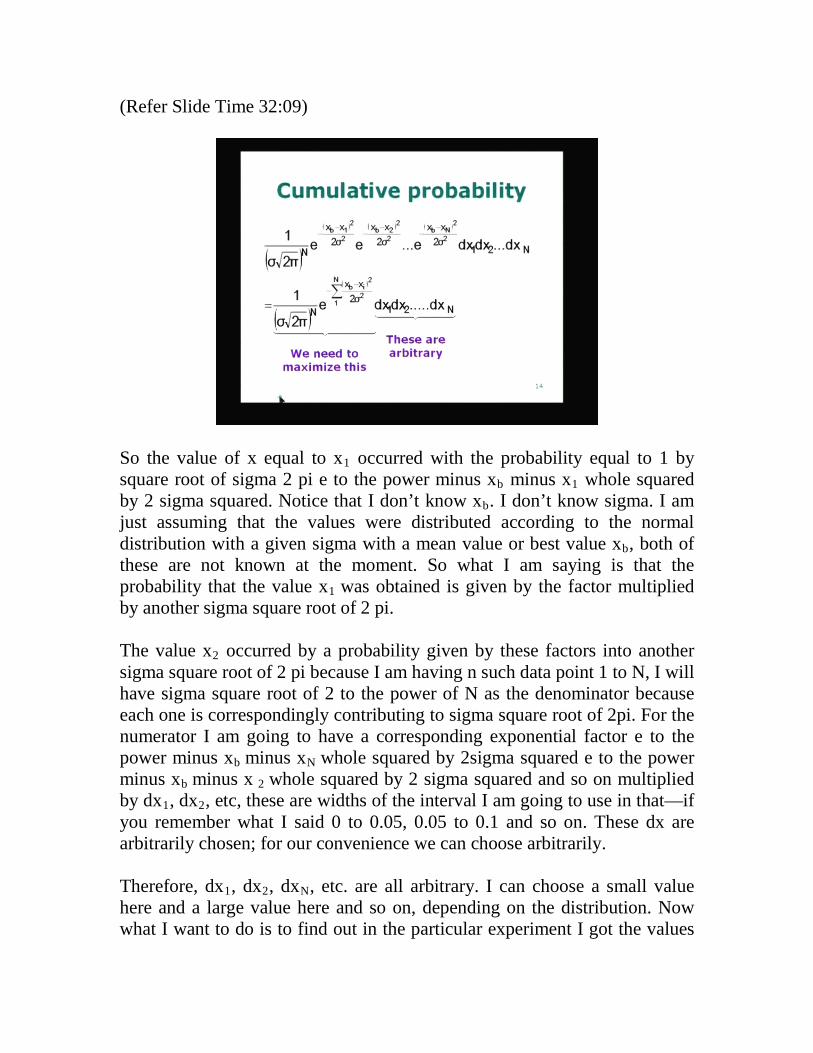
So the value of x equal to x1 occurred with the probability equal to 1 by square root of sigma 2 pi e to the power minus xb minus x1 whole squared by 2 sigma squared. Notice that I don’t know xb. I don’t know sigma. I am just assuming that the values were distributed according to the normal distribution with a given sigma with a mean value or best value xb, both of these are not known at the moment. So what I am saying is that the probability that the value x1 was obtained is given by the factor multiplied by another sigma square root of 2 pi. The value x2 occurred by a probability given by these factors into another sigma square root of 2 pi because I am having n such data point 1 to N, I will have sigma square root of 2 to the power of N as the denominator because each one is correspondingly contributing to sigma square root of 2pi. For the numerator I am going to have a corresponding exponential factor e to the power minus xb minus xN whole squared by 2sigma squared e to the power minus xb minus x 2 whole squared by 2 sigma squared and so on multiplied by dx1, dx2, etc, these are widths of the interval I am going to use in that—if you remember what I said 0 to 0.05, 0.05 to 0.1 and so on. These dx are arbitrarily chosen; for our convenience we can choose arbitrarily. Therefore, dx1, dx2, dxN, etc. are all arbitrary. I can choose a small value here and a large value here and so on, depending on the distribution. Now what I want to do is to find out in the particular experiment I got the values

x1, x2, xN. Why did I get these values? I got these values because this was the most probable. That means probability of getting that outcome, which is a set of measured values x1, x2, xN, was obtained only because it was highly probable; if it were not highly probable, how would I get those values? I should not get. Therefore I am going to make the hypothesis that this cumulative probability must be a maximum because I was able to get this outcome of the experiment as these values of x1 to xN are given by the data, which I have collected. So this is the basis for our analysis of the statistical nature of the data. Therefore there are 2 quantities, xb and sigma; both of them are not known at the moment. So I am going to make assumption that if I have to maximize this and you can see here that this can be written in a more succinct fashion: 1 by sigma square root of 2pi to the power N exponential of this, this, this is like adding e to the power of this plus this plus this. So I am showing it as e to the power minus sigma1 to N xb minus x1 whole square divided by 2sigma squared into the product of the intervals and because these are arbitrary, the cumulative probability will be maximum only if the factor (shown in slide) is maximized. 1 by sigma square root of 2pi to the power N e to the power of minus sigma1 to N xb minus xi whole squared divided by 2sigma square is going to be maximum. I am going to give two types of arguments here. I am going to first look at the maximization of this term by mathematically performing the derivative, taking the derivative and sending it to 0. Then I will also give a physical explanation of why we do that. So that will be explained on the board. I am going to use the board for this. Let me use the board and show how we are going to do this little bit of mathematics. If you go back to the slide, you will notice that we have 2 factors: the exponential factor into 1 by sigma square root of 2pi to the power N and exponential minus sigma i is equal to 1 to n sum of the squares divided by sigma squares, dx1, dx2 etc. Are the products on the other side? We need to look only at the first part. dx1, dx2 etc., dxN is not going to concern us. So let us write down, the cumulative probability (refer slide below) depends on 2 parameters: the value xb and sigma and this is only 1 factor. I am going to write this: 1 by sigma to the power of N square root of 2pi to the power N, exponential of minus sigma i is equal to 1 to N xb minus xi whole square divided by 2sigma square (refer formula in the slide). So we

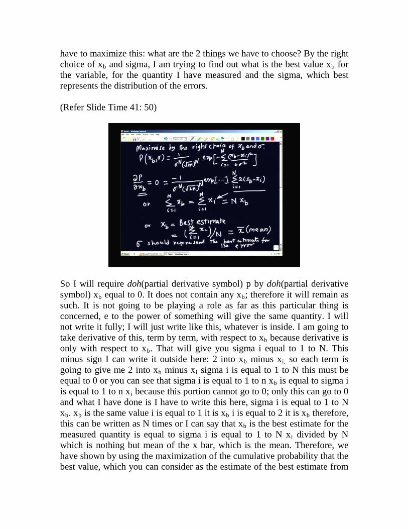
have to maximize this: what are the 2 things we have to choose? By the right choice of xb and sigma, I am trying to find out what is the best value xb for the variable, for the quantity I have measured and the sigma, which best represents the distribution of the errors. (Refer Slide Time 41: 50)

So I will require doh(partial derivative symbol) p by doh(partial derivative symbol) xb equal to 0. It does not contain any xb; therefore it will remain as such. It is not going to be playing a role as far as this particular thing is concerned, e to the power of something will give the same quantity. I will not write it fully; I will just write like this, whatever is inside. I am going to take derivative of this, term by term, with respect to xb because derivative is only with respect to xb. That will give you sigma i equal to 1 to N. This minus sign I can write it outside here: 2 into xb minus xi, so each term is going to give me 2 into xb minus xi sigma i is equal to 1 to N this must be equal to 0 or you can see that sigma i is equal to 1 to n xb is equal to sigma i is equal to 1 to n xi because this portion cannot go to 0; only this can go to 0 and what I have done is I have to write this here, sigma i is equal to 1 to N xb. xb is the same value i is equal to 1 it is xb i is equal to 2 it is xb therefore, this can be written as N times or I can say that xb is the best estimate for the measured quantity is equal to sigma i is equal to 1 to N xi divided by N which is nothing but mean of the x bar, which is the mean. Therefore, we have shown by using the maximization of the cumulative probability that the best value, which you can consider as the estimate of the best estimate from

the set of replicate data, is given by the mean, which is nothing but sigma i is equal to 1 to N xi divided by N. Let us now look at the evaluation of sigma. We have only done part of the way; we have looked at the best value. Now what is this sigma? Sigma should represent the best estimate for the error. Now I am going to look at how to obtain that. It can be done by simply taking the derivative with the sigma in to xb and then writing the expression and we will do that in the next page. (Refer Slide Time 46: 25)

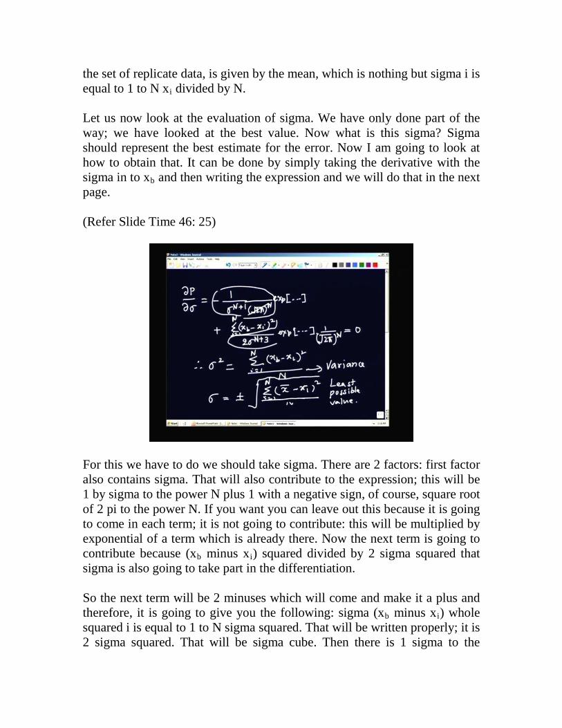
For this we have to do we should take sigma. There are 2 factors: first factor also contains sigma. That will also contribute to the expression; this will be 1 by sigma to the power N plus 1 with a negative sign, of course, square root of 2 pi to the power N. If you want you can leave out this because it is going to come in each term; it is not going to contribute: this will be multiplied by exponential of a term which is already there. Now the next term is going to contribute because (xb minus xi) squared divided by 2 sigma squared that sigma is also going to take part in the differentiation. So the next term will be 2 minuses which will come and make it a plus and therefore, it is going to give you the following: sigma (xb minus xi) whole squared i is equal to 1 to N sigma squared. That will be written properly; it is 2 sigma squared. That will be sigma cube. Then there is 1 sigma to the

power of N outside. So it will become N plus 3 and this must be multiplied by exponential whatever term we had and of course, 1 by square root of (2 pi) N. This must be equal to 0. So this exponential factor as well as 1 by 2pi factor is going to be common and it is not 0. Therefore this term and I am leaving out this, this term must be added to get 0 and therefore if you do that N plus 1 N plus 3, it will give sigma squared. We will get the value sigma squared, i is equal to 1 to N (xb minus xi) whole squared divided by N. That means we can also find out the standard deviation as the plus or minus square root of this quantity. This is nothing but the variance, which is always a positive quantity. Standard deviation can be plus or minus because the error could be in either negative direction or positive direction. We have already seen that and we have also seen that negative and positive errors must have similar probabilities and what we have found is very interesting and important relationship. xb is already determined; in the previous slide we have shown xb is nothing but x mean; so I can replace it by the mean value. So what this is indicating is that the variance sigma squared is this value and the standard deviation is this. In fact you can see that this is the least value for the variance or least value for the standard deviation. So we will make a note here of the least possible value. Why is it the least possible value? Because the variance is put into mean, the smallest you can think of; therefore, it is the least value. So with this background, let us go back to the slide show, which was indicating cumulative probability. This is where we took off and we went to the board to make a few calculations. Let us look at the next slide, which gives you what is called the least square principle.

(Refer Slide Time 46: 41)

So what we did is, by digressing and looking at the optimum or the best possible situation, by finding out the values of xb and sigma, the best estimate for the measured quantity and the best estimate for the variance of standard deviation it was done by taking the derivative of the cumulative property with respect to xb and sigma and then finding out what are the best estimates for the two quantities. If you remember what I said just before we took off from there, I said that variance is the least when you calculate variance with respect to the mean. That means, the least square principle means variance with respect to mean or the variance, which we calculate from the set of data you have got, must be the smallest we can take off. How do I do that? Let us look at the next slide, which gives me some another alternate way of looking at it. The alternate way of looking at it is to say the following: suppose I have been doing the experiment very carefully. I have taken care to choose proper instrument and so on, I have made sure that everything is properly arranged, no disturbances are allowed to interfere in our measurement. Then what should I expect? Like the sharp shooter, remember the last class I talked about the target practice? You had 3 people there: 1 who was good at target practice, target shooting, second person was like any of us, he did not have skills or whatever; the third person had skills but was not properly honed. So in the case of the person with best skills, you could see that all the values are coming within the first within the bull’s eye. So if I am a careful

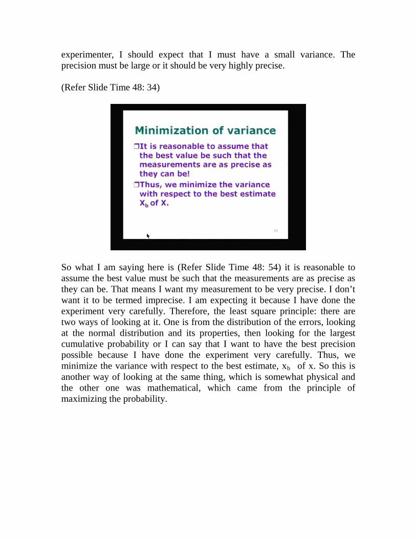
experimenter, I should expect that I must have a small variance. The precision must be large or it should be very highly precise. (Refer Slide Time 48: 34)

So what I am saying here is (Refer Slide Time 48: 54) it is reasonable to assume the best value must be such that the measurements are as precise as they can be. That means I want my measurement to be very precise. I don’t want it to be termed imprecise. I am expecting it because I have done the experiment very carefully. Therefore, the least square principle: there are two ways of looking at it. One is from the distribution of the errors, looking at the normal distribution and its properties, then looking for the largest cumulative probability or I can say that I want to have the best precision possible because I have done the experiment very carefully. Thus, we minimize the variance with respect to the best estimate, xb of x. So this is another way of looking at the same thing, which is somewhat physical and the other one was mathematical, which came from the principle of maximizing the probability.

(Refer Slide Time 49: 50)

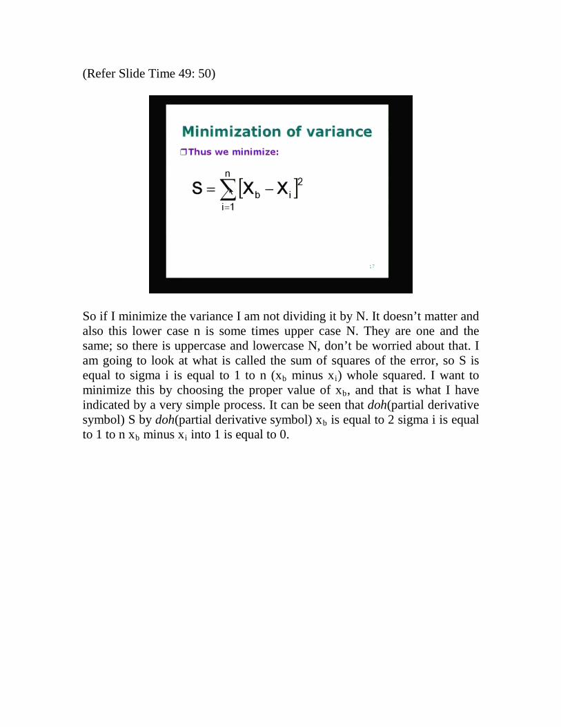
So if I minimize the variance I am not dividing it by N. It doesn’t matter and also this lower case n is some times upper case N. They are one and the same; so there is uppercase and lowercase N, don’t be worried about that. I am going to look at what is called the sum of squares of the error, so S is equal to sigma i is equal to 1 to n (xb minus xi) whole squared. I want to minimize this by choosing the proper value of xb, and that is what I have indicated by a very simple process. It can be seen that doh(partial derivative symbol) S by doh(partial derivative symbol) xb is equal to 2 sigma i is equal to 1 to n xb minus xi into 1 is equal to 0.

(Refer Slide Time 50: 20)

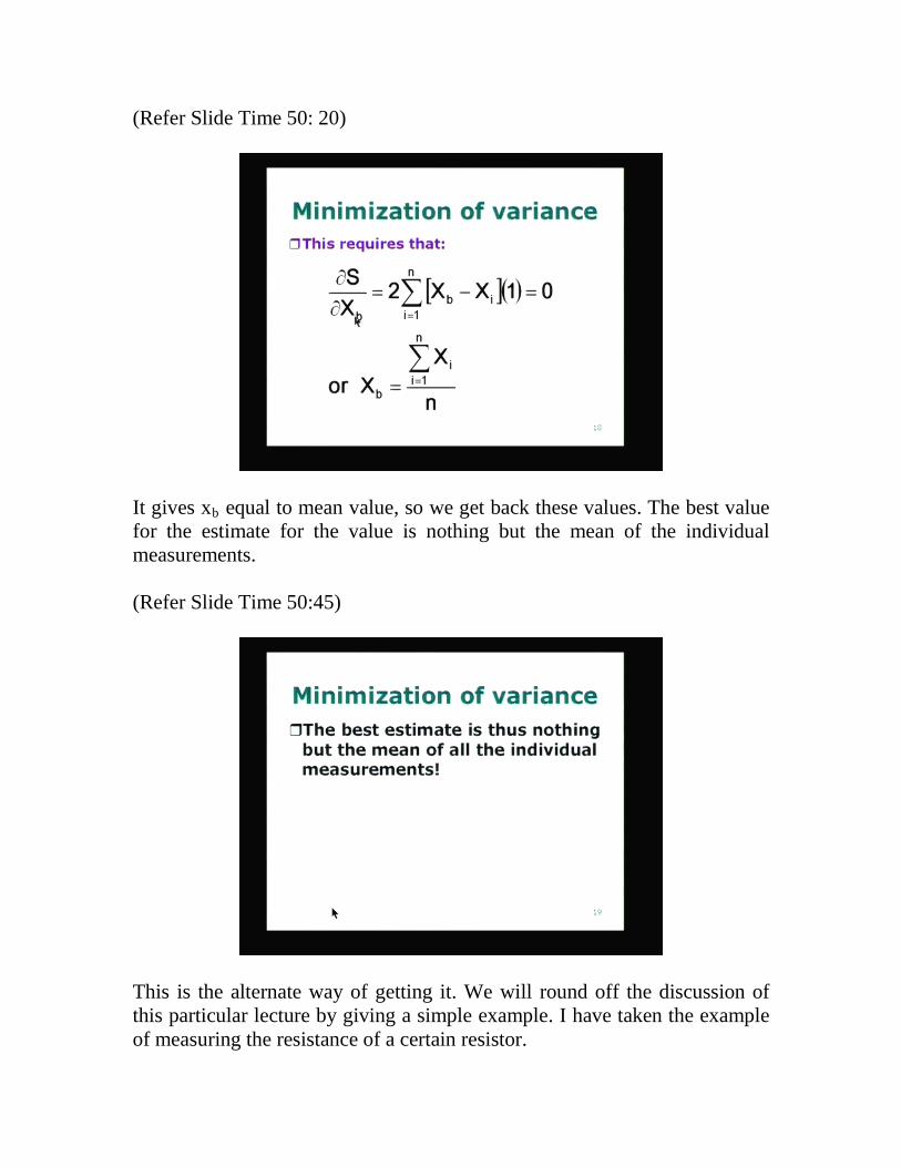
It gives xb equal to mean value, so we get back these values. The best value for the estimate for the value is nothing but the mean of the individual measurements. (Refer Slide Time 50:45)

This is the alternate way of getting it. We will round off the discussion of this particular lecture by giving a simple example. I have taken the example of measuring the resistance of a certain resistor.

(Refer Slide Time 50: 50)

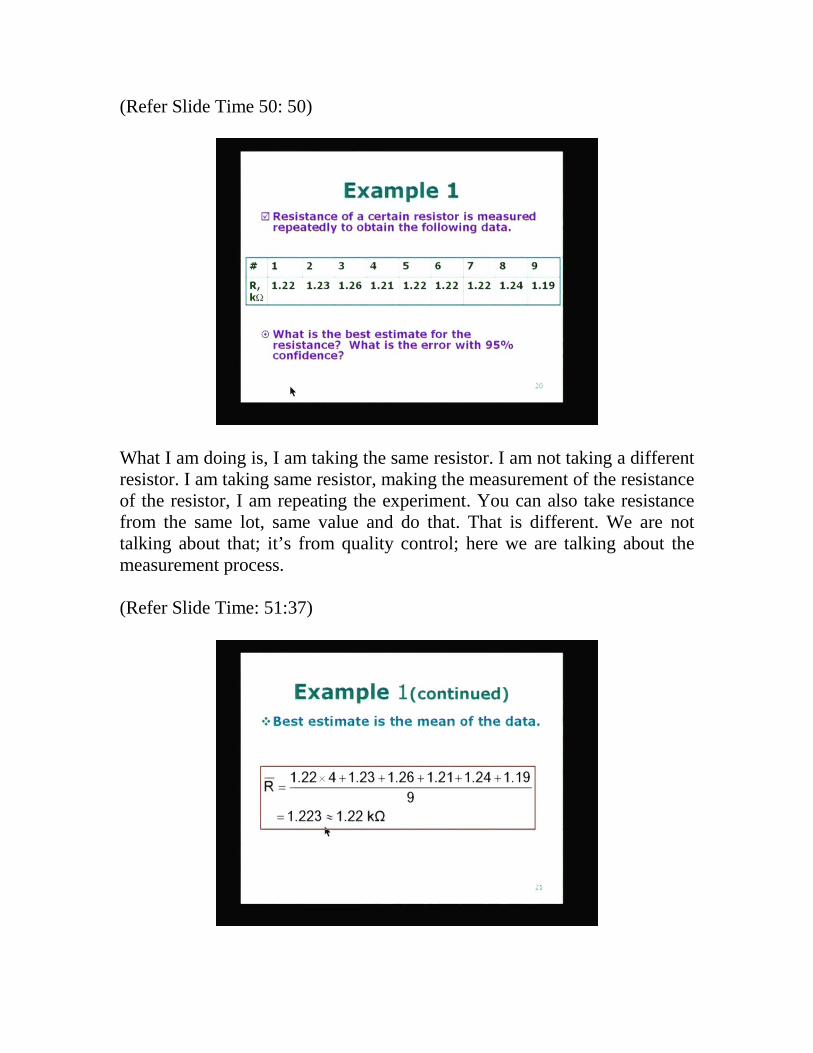
What I am doing is, I am taking the same resistor. I am not taking a different resistor. I am taking same resistor, making the measurement of the resistance of the resistor, I am repeating the experiment. You can also take resistance from the same lot, same value and do that. That is different. We are not talking about that; it’s from quality control; here we are talking about the measurement process. (Refer Slide Time: 51:37)

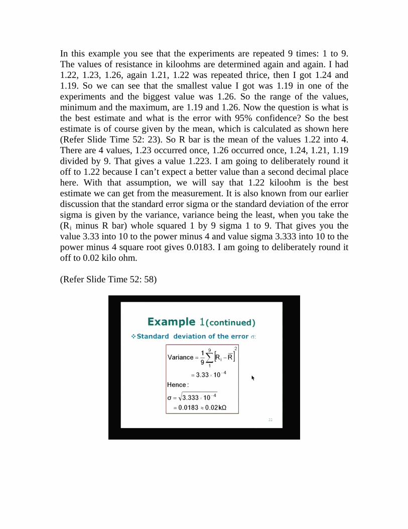
In this example you see that the experiments are repeated 9 times: 1 to 9. The values of resistance in kiloohms are determined again and again. I had 1.22, 1.23, 1.26, again 1.21, 1.22 was repeated thrice, then I got 1.24 and 1.19. So we can see that the smallest value I got was 1.19 in one of the experiments and the biggest value was 1.26. So the range of the values, minimum and the maximum, are 1.19 and 1.26. Now the question is what is the best estimate and what is the error with 95% confidence? So the best estimate is of course given by the mean, which is calculated as shown here (Refer Slide Time 52: 23). So R bar is the mean of the values 1.22 into 4. There are 4 values, 1.23 occurred once, 1.26 occurred once, 1.24, 1.21, 1.19 divided by 9. That gives a value 1.223. I am going to deliberately round it off to 1.22 because I can’t expect a better value than a second decimal place here. With that assumption, we will say that 1.22 kiloohm is the best estimate we can get from the measurement. It is also known from our earlier discussion that the standard error sigma or the standard deviation of the error sigma is given by the variance, variance being the least, when you take the (Ri minus R bar) whole squared 1 by 9 sigma 1 to 9. That gives you the value 3.33 into 10 to the power minus 4 and value sigma 3.333 into 10 to the power minus 4 square root gives 0.0183. I am going to deliberately round it off to 0.02 kilo ohm. (Refer Slide Time 52: 58)

(Refer Slide Time 53: 34)

Therefore I can say that with 95% confidence, the best value I can think of for the resistance is the value which I obtained in the previous slide (Refer Slide Time 52:23), 1.22 kiloohms plus or minus 1.96 sigma, which is 1.96 into 0.0183, which I am going to round off to 0.04—because it is 0.036—I am going to round it off to 0.04. I can say that for the value of the resistance, the best estimate is 1.22 kiloohms and error I can expect is 0.04 kiloohm, so 4 units in the second decimal place. I think we will stop here in this particular lecture, and in the next lecture we are going to look at an important aspect that is the propagation of errors. Once we have looked at this idea of propagation of errors, we will look at the regression analysis, which forms a very important part of presentation of data. Thank you.