meningioma expression analysis - dkfz.de · tions(basename = “meningioma”) after loading the...
TRANSCRIPT

Meningioma Expression Analysis
Gunnar Wrobel
February 26, 2004

Contents
1 Preprocessing 31.1 Introduction . . . . . . . . . . . . . . . . . . . . . . . . . . . . . . . . . . . . . 31.2 Requirements . . . . . . . . . . . . . . . . . . . . . . . . . . . . . . . . . . . . 31.3 Parameters . . . . . . . . . . . . . . . . . . . . . . . . . . . . . . . . . . . . . 31.4 Initializing . . . . . . . . . . . . . . . . . . . . . . . . . . . . . . . . . . . . . . 41.5 Loading data . . . . . . . . . . . . . . . . . . . . . . . . . . . . . . . . . . . . 41.6 Quality control . . . . . . . . . . . . . . . . . . . . . . . . . . . . . . . . . . . 71.7 Normalization . . . . . . . . . . . . . . . . . . . . . . . . . . . . . . . . . . . . 71.8 Filtering . . . . . . . . . . . . . . . . . . . . . . . . . . . . . . . . . . . . . . . 71.9 Combination of replicate data points . . . . . . . . . . . . . . . . . . . . . . . 8
2 Signature 102.1 Highly expressed genes . . . . . . . . . . . . . . . . . . . . . . . . . . . . . . . 102.2 Randomized data . . . . . . . . . . . . . . . . . . . . . . . . . . . . . . . . . . 102.3 Single gene plots . . . . . . . . . . . . . . . . . . . . . . . . . . . . . . . . . . 10
3 Classification 153.1 Primary shrunken centroid . . . . . . . . . . . . . . . . . . . . . . . . . . . . 153.2 Shrunken centroid on random data . . . . . . . . . . . . . . . . . . . . . . . . 153.3 ROC analysis . . . . . . . . . . . . . . . . . . . . . . . . . . . . . . . . . . . . 193.4 EASE Analysis . . . . . . . . . . . . . . . . . . . . . . . . . . . . . . . . . . . 33
4 IGF Pathway 344.1 ROC analysis . . . . . . . . . . . . . . . . . . . . . . . . . . . . . . . . . . . . 344.2 Correlated genes . . . . . . . . . . . . . . . . . . . . . . . . . . . . . . . . . . 384.3 Patients with upregulated IGF pathway . . . . . . . . . . . . . . . . . . . . . 38
5 WNT-signalling pathway 455.1 ROC analysis . . . . . . . . . . . . . . . . . . . . . . . . . . . . . . . . . . . . 455.2 Shrunken centroid . . . . . . . . . . . . . . . . . . . . . . . . . . . . . . . . . 46
6 Additional Analyses 546.1 Real-Time-Quantitative-PCR (RQ-PCR) . . . . . . . . . . . . . . . . . . . . 54
7 Conclusions 65
2

1 Preprocessing
1.1 Introduction
The amount of data generated by microarray expression profiling leads to a rather complexanalysis that is seldom easy to convey in the framework provided by a manuscript. To allowinterested researchers complete access to the analysis procedures employed for extractingthe results presented in the corresponding paper, all steps of the process from raw datato the final tables and figures are provided by this document. The document is writtenin Sweave-format [Leisch, 2002] and accompanied by the raw data. This file provides codein the R programming language [Ihaka & Gentleman, 1996], combined with comments inLATEX format. By processing the file using R, the code itself can be extracted or this PDFdocument can be generated to provide an overview of the analysis. Many of the functionsincluded were provided by the Bioconductor project [Project Bioconductor, 2000].
1.2 Requirements
In order to modify the analysis and/or produce this PDF, you need R 1.8.1 and the Biocon-ductor 1.3 Release. The package is guaranteed to produce this document given the specifiedenvironment. It will probably also be possible to use other versions of R though in case ofBioconducter you are advised to use the 1.3 release. Many of the Bioconductor packages donot yet have stable interfaces.
You will need the basic Bioconductor packages as well as the boot and the tree package.The boot and tree can be found on the (http://cran.at.r-project.org/) website .
1.3 Parameters
There are several options available to influence the calculations performed while generatingthe PDF document. Some of them can also be used to change the appearance of the file.The parameters that can be specified are given in Table 1.1.
To modify the parameters you can create a file parameters.txt in your working direc-tory. You will have to use a tab delimited format with the name of the option in the firstcolumn and the value for this option in the second column. This file will be read on startupof the package Meningioma. As an alternative you can use the command .retrieveBaseOp-tions(basename = “Meningioma”) after loading the package to retrieve a list that containsall available options and their current values. After changing some of the values according toyour demands you need to execute the command .setBaseOptions(options = yourOption-sList, basename = “Meningioma”) with the name yourOptionsList set to the name ofthe option list you retrieved. Please do also read the documentation to the .setBaseOptionsfunction.
3

To allow for a quick generation of the PDF document, time consuming steps are omittedby providing precalculated, intermediate datasets. The parameter file nevertheless allows torequest a recalculation of these data sets which will be necessary in case that prior steps orparameters of the analysis process have been modified. But please be aware that you willneed to activate the recalculation of the datasets. So in case you change a filter variablethere is no mechanism that automatically activates the necessary parameters. You will haveto additionally set any corresponding recalculation options.
Name Description ValuereadOriginalData The original data files will be read again. This should never be necessary,
but the original data has been included in the package. Setting this toFALSE will lead to a shorter calculation time.
FALSE
qualityPlots Activates the quality control plots for the document. The document willgrow significantly longer when set to TRUE
FALSE
normalize Leads to recalculation of the normalization. This might take a while andyou are advised to employ the newest vsn-package (v1.4) since the newcode runs much faster.
FALSE
invariant The fraction of genes that is assumed to show no variance in expression.This is used during variance stabilization for the selection of an invariantset of genes.
0.6
savedExprset This should be set to FALSE in case any of the prior steps of the analysishas been modified (loading of data, normalization or filtering). Otherwisethe filtering of the dataset is omitted and a precalculated data set is beingloaded.
FALSE
filterThreshold The fraction of genes with a bad quality score to be excluded from theanalysis. If you want to vary this setting you also need to set the previousoption to FALSE.
0.2
overallFilter The maximal fraction of samples for which a gene may have a filtered value(NA) in order to be accepted in the final analysis.
0.25
highGenes The number of genes with high expression that should be selected andpresented.
10
random This setting defines whether the random data should also be analysed andthe results presented.
TRUE
singlegenes Determines whether the plots for single genes should be given at differentlocations throughout the document.
TRUE
fullROC If set to TRUE all possible comparisons will be analyzed with ROC. TRUE
newROC This setting will allow a recalculation of the ROC datasets. Please becareful with this setting since it requires a large amount of memory and Iwas able to get repeated core dumps from R geenrating the ROC whithinthis document
FALSE
rocfilter The selection probability to be used for selecting genes from the ROCanalysis
0.4
Table 1.1: Parameter options available and their current settings.
1.4 Initializing
1.5 Loading data
In a first step all GenePix r© result files are loaded and combined to larger data tables thatcan be efficiently handled in R.
The rawfiles directory of the package holds all additional data files, also including theChips.txt file, which describes the experiments conducted on each slide. This table is readin first (see Table 1.2).> if (!errorOccurred) {
+ note <- "This holds only information about slides, not about"
4

+ note <- paste(note, "patients. Slide data still needs to be")
+ note <- paste(note, "combined for that (color switch).")
+ targets <- try(read.marrayInfo(fname = paste(OP$packagePath,
+ OP$dataFilePath, OP$sampleFile, sep = PSEP), info.id = 1:3,
+ label = 1, notes = note))
+ if (inherits(targets, "try-error")) {
+ warning("Cannot read Chips.txt file!")
+ errorOccurred <- TRUE
+ }
+ }
No. Chip Patient CyDye No. Chip Patient CyDye
1 Slide82.gpr MN109 Cy5 31 Slide67.gpr MN56B Cy52 Slide19.gpr MN109 Cy3 32 Slide90.gpr MN56B Cy33 Slide44.gpr MN27 Cy5 33 Slide43.gpr MN2 Cy54 Slide18.gpr MN27 Cy3 34 Slide10.gpr MN2 Cy35 Slide2.gpr MN40 Cy5 35 Slide58.gpr MN4 Cy56 Slide74.gpr MN40 Cy3 36 Slide12.gpr MN4 Cy37 Slide91.gpr MN119 Cy5 37 Slide26.gpr MN7 Cy58 Slide94.gpr MN119 Cy3 38 Slide99.gpr MN7 Cy39 Slide89.gpr MN113 Cy5 39 Slide73.gpr MN10 Cy510 Slide80.gpr MN113 Cy3 40 Slide81.gpr MN10 Cy311 Slide60.gpr MN30 Cy5 41 Slide11.gpr MN12 Cy512 Slide14.gpr MN30 Cy3 42 Slide3.gpr MN12 Cy313 Slide97.gpr MN41 Cy5 43 Slide17.gpr MN36 Cy514 Slide25.gpr MN41 Cy3 44 Slide87.gpr MN36 Cy315 Slide93.gpr MN69 Cy5 45 Slide8.gpr MN67 Cy516 Slide65.gpr MN69 Cy3 46 Slide84.gpr MN67 Cy317 Slide15.gpr MN42 Cy5 47 Slide95.gpr MN14 Cy518 Slide56.gpr MN42 Cy3 48 Slide83.gpr MN14 Cy319 Slide100.gpr MN62 Cy5 49 Slide47.gpr MN15 Cy520 Slide38.gpr MN62 Cy3 50 Slide34.gpr MN15 Cy321 Slide86.gpr MN45 Cy5 51 Slide7.gpr MN16 Cy522 Slide45.gpr MN45 Cy3 52 Slide55.gpr MN16 Cy323 Slide9.gpr MN47 Cy5 53 Slide27.gpr MN37 Cy524 Slide40.gpr MN47 Cy3 54 Slide96.gpr MN37 Cy325 Slide63.gpr MN63B Cy5 55 Slide61.gpr MN19 Cy526 Slide36.gpr MN63B Cy3 56 Slide13.gpr MN19 Cy327 Slide98.gpr MN34 Cy5 57 Slide52.gpr MN20 Cy528 Slide35.gpr MN34 Cy3 58 Slide37.gpr MN20 Cy329 Slide68.gpr MN58 Cy5 59 Slide39.gpr MN22 Cy530 Slide54.gpr MN58 Cy3 60 Slide16.gpr MN22 Cy3
Table 1.2: Experimental results to be loaded.
Table 1.2 defines the chip files that have to be loaded during the analysis process. Thedata files included here only represent the set of chips that were successfully hybridized.About 10% gave results with inacceptable quality either due to problems of the RNA sampleor the hybridization itself.
5

> if (!errorOccurred) {
+ y <- try(readLines(paste(OP$packagePath, OP$dataFilePath,
+ OP$layoutFile, sep = PSEP), n = 100))
+ skip <- intersect(grep("ID", y), grep("Name", y))[1] - 1
+ if (inherits(y, "try-error")) {
+ warning("Cannot read layout file!")
+ errorOccurred <- TRUE
+ }
+ }
This section determines the header length of the layout file loaded in the next step.
> if (!errorOccurred) {
+ note <- "The layout holds additional information about"
+ note <- paste(note, "the plates the probes were spotted from.")
+ layout <- try(read.marrayLayout(paste(OP$packagePath, OP$dataFilePath,
+ OP$layoutFile, sep = PSEP), 8, 4, 19, 19, pl.col = 6,
+ ctl.col = 4, sub.col = NULL, notes = note, skip = skip))
+ note <- "The genenames object holds additional"
+ note <- paste(note, "information about the genes on the array.")
+ genenames <- try(read.marrayInfo(fname = paste(OP$packagePath,
+ OP$dataFilePath, OP$layoutFile, sep = PSEP), info.id = 4:17,
+ label = 5, skip = skip, notes = note))
+ if (inherits(layout, "try-error") | inherits(genenames, "try-error")) {
+ warning("Cannot read layout file!")
+ errorOccurred <- TRUE
+ }
+ }
Here, the layout of the chip is included to have all necessary information about the genesavailable. Additional gene information is saved in a marrayInfo object (genenames). Thisinformation is also read from the GAL file. Usually, this file does not carry more informationthan name and ID of a gene, but here, additional information has been pasted into the file.
> if (!errorOccurred) {
+ note <- "This holds information about patients."
+ patients <- try(read.marrayInfo(fname = paste(OP$packagePath,
+ OP$dataFilePath, OP$patientsFile, sep = PSEP), info.id = 1:61,
+ label = 1, notes = note))
+ if (inherits(patients, "try-error")) {
+ warning("Cannot read patient file!")
+ errorOccurred <- TRUE
+ }
+ }
The data which are available for each patient are read into the marrayInfo objectpatients. The data include informations about diagnosis, sex, age, CGH-data and someadditional clinical parameters that were measured.
> if (!errorOccurred) {
+ if (OP$readOriginalData) {
+ try(memory.limit(2000))
+ note <- "Meningioma dataset"
+ fPath <- paste(OP$packagePath, OP$dataFilePath, sep = PSEP)
+ data <- try(read.GenePix(as.character(maInfo(targets)[,
+ 1]), path = fPath, name.Gf = "F532 Median", name.Gb = "B532 Median",
+ name.Rf = "F635 Median", name.Rb = "B635 Median",
+ name.W = "Flags", layout = layout, gnames = genenames,
+ targets = targets, notes = note))
+ datamean <- try(read.GenePix(as.character(maInfo(targets)[,
+ 1]), path = fPath, name.Gf = "F532 Mean", name.Gb = "B532 Mean",
+ name.Rf = "F635 Mean", name.Rb = "B635 Mean", name.W = "Flags",
+ layout = layout, gnames = genenames, targets = targets,
+ notes = "Meningioma dataset"))
+ if (inherits(data, "try-error") | inherits(datamean,
+ "try-error")) {
+ warning("Cannot read data files!")
+ errorOccurred <- TRUE
+ }
+ }
+ else {
+ data(rawdata)
+ data(rawdatamean)
+ }
+ }
Finally, this chunk of code reads in all primary chip data.
6

1.6 Quality control
The parameter file is currently set to omit the quality control plots. They can be easilyadded by setting the parameter QualityPlots to TRUE. The calculations will take longerthough and the size of this document grows significantly.
1.7 Normalization
For normalization the variance stabilization method [Huber et al., 2002] is employed. Thiscalculation takes a serious amount of time on a dataset like the one provided here. To avoidthe calculations here, the normalized data is provided as a precalculated dataset withinthe package and just loaded here. To verify the normalization or include modifications tothe analysis, the normalize parameter can be set to TRUE as described above. But thecalculation might easily run over several hours, depending on the speed of the machine.
Since the patient samples have been hybridized to a generic control, only 60% of thegenes are assumed to show relatively constant expression. This parameter is needed for thevariance stabilization [Huber et al., 2002].
> if (!errorOccurred) {
+ if (OP$normalize) {
+ yv <- vsn(cbind(maGf(data) - maGb(data), maRf(data) -
+ maRb(data)), lts.quantile = OP$invariant)
+ normG <- exprs(yv)[, 1:60]
+ normR <- exprs(yv)[, 61:120]
+ norm <- normR - normG
+ }
+ else {
+ data(norm)
+ }
+ }
1.8 Filtering
The data are filtered according to three different quality criteria for each spot. The intensityof each spot is considered, as well as the standard deviation of log ratios between replicatespots and the median to mean ratio as a criterium to judge the homogeneity of the spot.All three parameters are joined to one value describing the spot quality.
> if (!errorOccurred) {
+ if (!OP$savedExprset) {
+ invRank <- function(X) length(X) - rank(X) + 1
+ simpleScale <- function(X) X/max(X, na.rm = TRUE)
+ checkNames <- function(X) {
+ naClones <- c("Error", "na", "blank", "free space",
+ "empty", "n/a", "Blank", "None", "no clone",
+ "no clone", "none")
+ check <- NULL
+ for (i in 1:length(X)) {
+ check <- c(check, any(X[i] == naClones))
+ }
+ check
+ }
+ cN <- data@maGnames@maInfo$Name
+ cI <- data@maGnames@maInfo$ID
+ norm[checkNames(cI) | checkNames(cN), ] <- NA
+ norm[cI == "Control", ] <- NA
+ norm[maW(data) < 0] <- NA
+ int2bkg <- (maGf(data)/maGb(data)) + (maRf(data)/maRb(data))
+ int2bkg[is.na(norm)] <- NA
+ intRank <- apply(int2bkg, 2, rank)
+ intRank[is.na(norm)] <- NA
+ intRank <- apply(intRank, 2, simpleScale)
+ meanMedian <- (maGf(datamean) - maGb(datamean))/(maGf(data) -
+ maGb(data)) * (maRf(datamean) - maRb(datamean))/(maRf(data) -
+ maRb(data))
+ meanMedian[is.na(norm)] <- NA
7

+ meanMedianRank <- apply(meanMedian, 2, invRank)
+ meanMedianRank[is.na(norm)] <- NA
+ meanMedianRank <- apply(meanMedianRank, 2, simpleScale)
+ normSD <- matrix(nrow = dim(norm)[1], ncol = dim(norm)[2])
+ for (i in 1:(dim(norm)[2])) {
+ for (j in 1:(dim(norm)[1]/2)) {
+ a <- sd(c(norm[j, i], norm[dim(norm)[1]/2 + j,
+ i]), na.rm = TRUE)
+ normSD[j, i] <- a
+ normSD[dim(norm)[1]/2 + j, i] <- a
+ }
+ }
+ normSD[is.na(norm)] <- NA
+ normSDRank <- apply(normSD, 2, invRank)
+ normSDRank[is.na(norm)] <- NA
+ normSDRank <- apply(normSDRank, 2, simpleScale)
+ final <- intRank * meanMedianRank * normSDRank
+ final[is.na(norm)] <- NA
+ finalRank <- apply(final, 2, rank)
+ finalRank[is.na(norm)] <- NA
+ finalRank <- apply(finalRank, 2, simpleScale)
+ norm[finalRank < OP$filterThreshold] <- NA
+ }
+ }
1.9 Combination of replicate data points
As a last step of data preprocessing, replicate spots and colorswitch experiments are com-bined to a final expression value. Additionally, all genes that lack a ratio value in more than25% of the samples are removed from further analysis. On basis of the final dataset tworandom datasets are created: The first one is generated by creating a matrix the same sizeas the original and filling it randomly with values from the real dataset. The same positionsthat were filtered in the original dataset are also filtered in this randomized set. The seconddataset simply randomizes each gene. Each randomized gene is generated by selecting itsvalues from the original data vector (including filtered values).
> if (!errorOccurred) {
+ if (!OP$savedExprset) {
+ exprData <- matrix(nrow = dim(norm)[1]/2, ncol = dim(norm)[2])
+ for (i in 1:(dim(norm)[2])) {
+ for (j in 1:(dim(norm)[1]/2)) {
+ exprData[j, i] <- mean(c(norm[j, i], norm[dim(norm)[1]/2 +
+ j, i]), na.rm = TRUE)
+ }
+ }
+ exprData <- (exprData[, seq(from = 1, to = 60, by = 2)] -
+ exprData[, seq(from = 2, to = 60, by = 2)])/2
+ cN <- as.character(data@maGnames@maInfo$GeneSymbol)
+ cN[cN == ""] <- paste("ImageID:", as.character(data@maGnames@maInfo$ID[cN ==
+ ""]))
+ colnames(exprData) <- as.character(maInfo(targets)[seq(from = 1,
+ to = 60, by = 2), 2])
+ rownames(exprData) <- as.character(cN)[1:(length(cN)/2)]
+ pool <- as.vector(exprData[!is.na(exprData)])
+ randData <- exprData
+ a <- dim(exprData)[1]
+ b <- dim(exprData)[2]
+ for (i in 1:b) {
+ for (j in 1:a) {
+ randData[j, i] <- pool[as.integer(runif(1, 1,
+ length(pool)) + 0.5)]
+ }
+ }
+ randData[is.na(exprData)] <- NaN
+ randGData <- exprData
+ a <- dim(exprData)[1]
+ b <- dim(exprData)[2]
+ for (i in 1:a) {
+ for (j in 1:b) {
+ randGData[i, j] <- exprData[i, as.integer(runif(1,
+ 1, b) + 0.5)]
+ }
+ }
+ countEntries <- function(X) length(X) - sum(as.integer(is.na(X)))
+ countrow <- apply(exprData, 1, countEntries)
+ thres <- ncol(exprData) * (1 - OP$overallFilter)
+ newData <- exprData[countrow > thres, ]
+ centeredData <- t(t(newData) - apply(newData, 2, median,
8

+ na.rm = TRUE))
+ pd <- as.data.frame(maInfo(patients))
+ pl <- as.list(colnames(pd))
+ names(pl) <- names(pd)
+ pD <- new("phenoData", pData = pd, varLabels = pl)
+ note <- "The normalized and filtered dataset"
+ dataset <- new("exprSet", exprs = centeredData, phenoData = pD,
+ notes = note)
+ a <- colnames(pData(phenoData(dataset)))
+ dataset@phenoData@varLabels <- as.list(a)
+ genes <- (genenames[1:(length(maInfo(genenames)[, 4])/2)])[countrow >
+ thres]
+ countrow <- apply(randData, 1, countEntries)
+ thres <- ncol(randData) * (1 - OP$overallFilter)
+ newData <- randData[countrow > thres, ]
+ centeredData <- t(t(newData) - apply(newData, 2, median,
+ na.rm = TRUE))
+ note <- "The normalized and filtered complete random dataset"
+ randdataset <- new("exprSet", exprs = centeredData, phenoData = pD,
+ notes = note)
+ a <- colnames(pData(phenoData(randdataset)))
+ randdataset@phenoData@varLabels <- as.list(a)
+ randgenes <- (genenames[1:(length(maInfo(genenames)[,
+ 4])/2)])[countrow > thres]
+ countrow <- apply(randGData, 1, countEntries)
+ thres <- ncol(randGData) * (1 - OP$overallFilter)
+ newData <- randGData[countrow > thres, ]
+ centeredData <- t(t(newData) - apply(newData, 2, median,
+ na.rm = TRUE))
+ note <- "The normalized and filtered genewise random dataset"
+ randGdataset <- new("exprSet", exprs = centeredData,
+ phenoData = pD, notes = note)
+ tmp <- as.list(colnames(pData(phenoData(randGdataset))))
+ randGdataset@phenoData@varLabels <- tmp
+ randGgenes <- (genenames[1:(length(maInfo(genenames)[,
+ 4])/2)])[countrow > thres]
+ }
+ else {
+ data(genes)
+ data(dataset)
+ data(randgenes)
+ data(randdataset)
+ data(randGgenes)
+ data(randGdataset)
+ }
+ }
9

2 Signature
2.1 Highly expressed genes
While the comparison of expression levels between samples and the control RNA does notallow any functional insight, genes that were found highly expressed in meningioma samplesas compared to the reference should represent a characteristic profile for the studied celltype. The highly expressed genes are selected by their median over all samples.
> if (!errorOccurred) {
+ geneValueHigh <- dataset[order(rank(esApply(dataset, 1, median,
+ na.rm = TRUE)), decreasing = TRUE), ]
+ geneInfoHigh <- genes[order(rank(esApply(dataset, 1, median,
+ na.rm = TRUE)), decreasing = TRUE)]
+ }
Several of the genes shown in Figure 2.1 are well known to be expressed in menin-gioma. This is the case for PGTDS [Yamashima et al., 1997, Kawashima et al., 2001],CLU [Shinoura et al., 1994], MGP [Hirota et al., 1995], MMP12 [Kachra et al., 1999], VIM[NG & Wong, 1993], and TIMP1 [Kachra et al., 1999]. Since no healthy meningeal tissuewas included in the profiling, it is impossible to derive any functional conclusions about thetumors based on the high expression of these genes. The genes might only represent thesignature of healthy meningeal tissue and could perhaps have no relation to the pathologi-cal state. Nevertheless, the correct identification of known aspects about meningioma geneexpression underlines the reliability of the data.
2.2 Randomized data
Figure 2.2 shows the same analysis for the randomized data set. As expected, the valuesare lower simply demonstrating that the initial data set is not randomly distributed.
2.3 Single gene plots
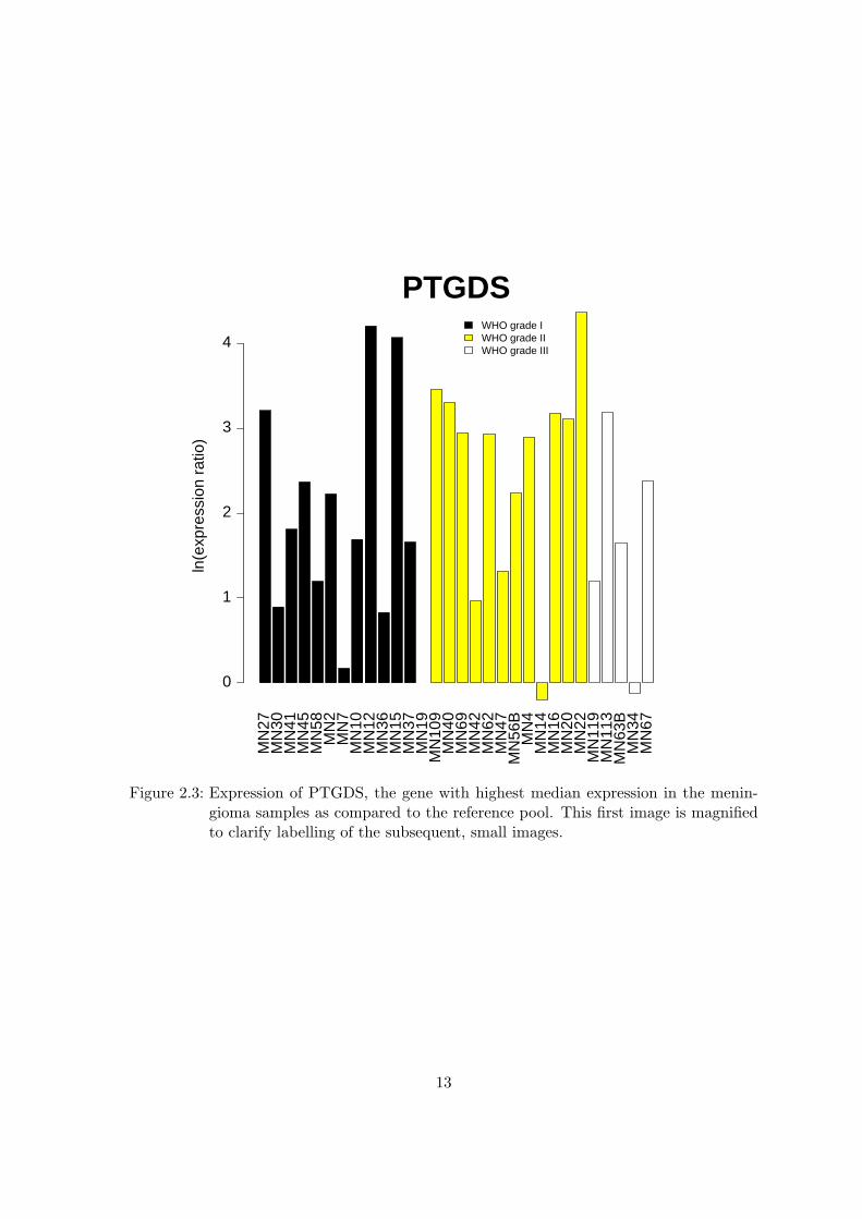
Figures 2.3 and 2.4 show the expression over all samples for each of the highly expressedgenes.
10

●
●
●
●
●
●
●
●
Highly expressed genes
ln(e
xpre
ssio
n ra
tio)
PT
GD
S
CLU
BA
D
MG
P
LIG
1
AN
XA
2
MM
P12
VIM
TIM
P1
CC
ND
1
0
1
2
3
4
Figure 2.1: The genes showing highest median expression in the meningioma samples ascompared to the control RNA. The central line denotes the median of expressionover all samples while the box is drawn from the upper to the lower quartile.The lines extending from the boxes represent the first value below the lowerquartile plus 1.5 times the interquartile range, respectively the first value abovethe upper quartile plus 1.5 times the interquartile range. The dots show outlierslying outside these boundaries.
11

●
●
●
●●●
●
●
●
●
●
●
●
●
●
●
●
●
●
●
●
●
●
●
●
●
●
Highly expressed genes (random data set)
ln(e
xpre
ssio
n ra
tio)
HS
P10
5B
GLG
1
RB
BP
7
RA
NB
P1
LOC
5114
7
PA
M
ZN
F14
8
CD
80
ET
S2
−2
−1
0
1
2
Figure 2.2: Genes with high expression using a randomized data set. Details of the boxplotare given in Figure 2.1.
12
MN
27M
N30
MN
41M
N45
MN
58M
N2
MN
7M
N10
MN
12M
N36
MN
15M
N37
MN
19M
N10
9M
N40
MN
69M
N42
MN
62M
N47
MN
56B
MN
4M
N14
MN
16M
N20
MN
22M
N11
9M
N11
3M
N63
BM
N34
MN
67
PTGDS
ln(e
xpre
ssio
n ra
tio)
0
1
2
3
4WHO grade IWHO grade IIWHO grade III
Figure 2.3: Expression of PTGDS, the gene with highest median expression in the menin-gioma samples as compared to the reference pool. This first image is magnifiedto clarify labelling of the subsequent, small images.
13

MN
27M
N30
MN
41M
N45
MN
58M
N2
MN
7M
N10
MN
12M
N36
MN
15M
N37
MN
19M
N10
9M
N40
MN
69M
N42
MN
62M
N47
MN
56B
MN
4M
N14
MN
16M
N20
MN
22M
N11
9M
N11
3M
N63
BM
N34
MN
67
CLU
ln(e
xpre
ssio
n ra
tio)
0.0
0.5
1.0
1.5
2.0
2.5
MN
27M
N30
MN
41M
N45
MN
58M
N2
MN
7M
N10
MN
12M
N36
MN
15M
N37
MN
19M
N10
9M
N40
MN
69M
N42
MN
62M
N47
MN
56B
MN
4M
N14
MN
16M
N20
MN
22M
N11
9M
N11
3M
N63
BM
N34
MN
67
BAD
ln(e
xpre
ssio
n ra
tio)
0.0
0.5
1.0
1.5
2.0
2.5
MN
27M
N30
MN
41M
N45
MN
58M
N2
MN
7M
N10
MN
12M
N36
MN
15M
N37
MN
19M
N10
9M
N40
MN
69M
N42
MN
62M
N47
MN
56B
MN
4M
N14
MN
16M
N20
MN
22M
N11
9M
N11
3M
N63
BM
N34
MN
67
MGP
ln(e
xpre
ssio
n ra
tio)
0.0
0.5
1.0
1.5
2.0
2.5
MN
27M
N30
MN
41M
N45
MN
58M
N2
MN
7M
N10
MN
12M
N36
MN
15M
N37
MN
19M
N10
9M
N40
MN
69M
N42
MN
62M
N47
MN
56B
MN
4M
N14
MN
16M
N20
MN
22M
N11
9M
N11
3M
N63
BM
N34
MN
67
LIG1
ln(e
xpre
ssio
n ra
tio)
0.0
0.5
1.0
1.5
2.0
MN
27M
N30
MN
41M
N45
MN
58M
N2
MN
7M
N10
MN
12M
N36
MN
15M
N37
MN
19M
N10
9M
N40
MN
69M
N42
MN
62M
N47
MN
56B
MN
4M
N14
MN
16M
N20
MN
22M
N11
9M
N11
3M
N63
BM
N34
MN
67
ANXA2
ln(e
xpre
ssio
n ra
tio)
0.0
0.5
1.0
1.5
MN
27M
N30
MN
41M
N45
MN
58M
N2
MN
7M
N10
MN
12M
N36
MN
15M
N37
MN
19M
N10
9M
N40
MN
69M
N42
MN
62M
N47
MN
56B
MN
4M
N14
MN
16M
N20
MN
22M
N11
9M
N11
3M
N63
BM
N34
MN
67
MMP12
ln(e
xpre
ssio
n ra
tio)
0.0
0.5
1.0
1.5
2.0
MN
27M
N30
MN
41M
N45
MN
58M
N2
MN
7M
N10
MN
12M
N36
MN
15M
N37
MN
19M
N10
9M
N40
MN
69M
N42
MN
62M
N47
MN
56B
MN
4M
N14
MN
16M
N20
MN
22M
N11
9M
N11
3M
N63
BM
N34
MN
67
VIM
ln(e
xpre
ssio
n ra
tio)
0.0
0.5
1.0
1.5
2.0
MN
27M
N30
MN
41M
N45
MN
58M
N2
MN
7M
N10
MN
12M
N36
MN
15M
N37
MN
19M
N10
9M
N40
MN
69M
N42
MN
62M
N47
MN
56B
MN
4M
N14
MN
16M
N20
MN
22M
N11
9M
N11
3M
N63
BM
N34
MN
67
TIMP1
ln(e
xpre
ssio
n ra
tio)
0.0
0.5
1.0
1.5
2.0
2.5
MN
27M
N30
MN
41M
N45
MN
58M
N2
MN
7M
N10
MN
12M
N36
MN
15M
N37
MN
19M
N10
9M
N40
MN
69M
N42
MN
62M
N47
MN
56B
MN
4M
N14
MN
16M
N20
MN
22M
N11
9M
N11
3M
N63
BM
N34
MN
67
CCND1
ln(e
xpre
ssio
n ra
tio)
0.0
0.5
1.0
1.5
2.0
Figure 2.4: Single genes showing high expression in comparison to the reference RNA pool.
14

3 Classification
3.1 Primary shrunken centroid
The assumption underlying the experiment presented here was that the different tumorgrades can be easily classified by a method like hierarchical clustering or shrunken centroids.The latter method is used here to learn a classifier for the three different meningioma grades.> WHO <- pData(phenoData(dataset))$WHOgrade
> mData <- pamr.knnimpute(list(x = exprs(dataset), y = WHO))
> mData$genenames <- paste(as.character(maInfo(genes)[, 4]), " (",
+ as.character(maInfo(genes)[, 6]), ")", sep = "")
> mData$genenames[mData$genenames == " ()"] <- paste("ImageID:",
+ as.character(maInfo(genes)[mData$genenames == "", 7]))
> mData$samplelabels <- colnames(mData$x)
> train <- pamr.train(mData, n.threshold = 100)
> cv <- pamr.cv(train, mData, folds = balanced.folds(train$y, nfold = 13))
Figure 3.1 depicts the dependance of the misclassification error on the degree of shrink-age. The graph clearly shows that there is no useful separation obtained. The cross validatederror is in the range of 40% which is not acceptable for classification purposes.
By limiting the comparison to tumor samples of grade I and grade III the method is ableto provide a stable centroid allowing to classify the samples.> renData <- exprs(dataset)
> rownames(renData) <- as.character(as.vector(maInfo(genes)[, 4]))
> mData2 <- pamr.knnimpute(list(x = renData[, WHO != "II"], y = WHO[WHO !=
+ "II"]))
> mData2$genenames <- as.character(maInfo(genes)[, 4])
> mData2$location <- as.character(maInfo(genes)[, 6])
> mData2$genenames[mData2$genenames == ""] <- paste("ImageID:",
+ as.character(maInfo(genes)[mData2$genenames == "", 7]))
> mData2$samplelabels <- colnames(mData2$x)
> train2 <- pamr.train(mData2, n.threshold = 100)
> cv2 <- pamr.cv(train2, mData2, folds = balanced.folds(train2$y,
+ nfold = 13))
> t2 <- 2
> pamr.confusion(cv2, t2)
I III Class Error rate
I 12 1 0.07692308
III 1 4 0.20000000
Overall error rate= 0.109
Figure 3.2 shows the corresponding misclassification error and Figure 3.3 depicts theclass probabilities after choosing a threshold of 2.0. This looks a lot more promising, but onthe other hand the tumors are separated by one grade and the number of tumors in gradeIII is too low to obtain a generalized classifier. Still the genes included in the centroids (seeFigure 3.4) are already interesting. They will be mentioned again later.
3.2 Shrunken centroid on random data
The shrunken centroid analysis based on the randomized data set demonstrates that novalid classification can be derived and is intended to yield a measure for the maximal mis-classification we can expect from our data.
15

0.0 0.5 1.0 1.5 2.0 2.5 3.0
Value of threshold
Mis
clas
sific
atio
n er
ror
2088 1891 1453 954 586 318 184 107 63 41 23 17 11 8 6 3 3 2 2 2 2 2 2 0
Number of genes
0.0
0.2
0.4
0.6
0.8
0.0 0.5 1.0 1.5 2.0 2.5 3.0
Value of threshold
Mis
clas
sific
atio
n er
ror
2088 1891 1453 954 586 318 184 107 63 41 23 17 11 8 6 3 3 2 2 2 2 2 2 0
Number of genes
0.0
0.4
0.8
IIIIII
Figure 3.1: Shrunken centroid analysis of all three tumor grades. The dependance of themisclassification error on the amount of shrinkage is depicted for the completeset of samples (top) and for each tumor grade alone (bottom).
16

0 1 2 3 4
Value of threshold
Mis
clas
sific
atio
n er
ror
2088 1308 756 380 179 94 60 28 17 11 5 3 2 2 2 2 2 1 1 1 1 1 1 1 1 1 1
Number of genes
0.0
0.2
0.4
0.6
0.8
0 1 2 3 4
Value of threshold
Mis
clas
sific
atio
n er
ror
2088 1308 756 380 179 94 60 28 17 11 5 3 2 2 2 2 2 1 1 1 1 1 1 1 1 1 1
Number of genes
0.0
0.4
0.8
IIII
Figure 3.2: Shrunken centroid analysis of benign and anaplastic meningiomas. The depen-dance of the misclassification error on the amount of shrinkage is depicted forthe complete set of samples (top) and for each tumor grade alone (bottom).
17

Cross−validated class probabilities
Cro
ss−
valid
ated
pro
babi
litie
s
MN
27
MN
30
MN
41
MN
45
MN
58
MN
2
MN
7
MN
10
MN
12
MN
36
MN
15
MN
37
MN
19
MN
119
MN
113
MN
63B
MN
34
MN
67
0%20
%40
%60
%80
%10
0%
0%20
%40
%60
%80
%10
0%
●
●
●●
●
●
●
●
●
●
●●
●
●
●
●
●
●
●
●
●●
●
●
●
●
●
●
●●
●
●
●
●
●
●
Class I Class III
Figure 3.3: Shrunken centroid analysis of benign and anaplastic meningiomas. The classprobabilities for each sample are depicted.
I III
ENC1
CCND1
CDK5R1
CENPF
LDHB
AKT3
IGFBP3
(5q12−q13.3)
(11q13)
(17q11.2)
(1q32−q41)
(12p12.2−p12.1)
(1q43−q44)
(7p13−p12)
Figure 3.4: Shrunken centroid analysis of benign and anaplastic meningiomas. The genescomposing the two centroids are shown in combination with a representation(horizontal lines) of their corresponding values in the centroids. These lines rep-resent magnitude of the value and whether the gene is up- or down-regulated(right, respectively left orientation) in the corresponding class.
18

> rt <- 1.0
> pamr.confusion(rcv,rt)
I II III Class Error rate
I 6 7 0 0.5384615
II 8 4 0 0.6666667
III 1 4 0 1.0000000
Overall error rate= 0.621
The misclassification error for all classes is rather high (Figure 3.5).
3.3 ROC analysis
The shrunken centroid classification suggests that there is no strict border between theclasses. Thus, it will be harder to identify single genes that are responsible for tu-mor progression. There may exist a variety of reasons why the histological classifi-cation does not perfectly match to specific molecular states of the tumor cells. Thiscould for example be related to the high number of different meningioma subtypes[Kleihues et al., 1993, Louis et al., 2000] or reflect different pathomechanisms.
To allow for the selection of genes with relevance to tumor progression under these cir-cumstances, receiver-operator-curves (ROC) were employed. The method is comparable toa parametric Mann-Whitney test, but preferentially selects genes that show strong differen-tial expression in a subset of patients of one class [Pepe et al., 2003] instead of genes thatare homogeneously expressed within a class though differently expressed between classes.
Any selection of genes based on techniques that are applied genewise will also identifyfalse positive genes because of the high number of datapoints per sample that result from amicroarray experiment. While the ROC method has been shown to result in a list of genesthat is strongly enriched with genes truly differentially expressed [Pepe et al., 2003], thistype of analysis cannot be the basis for a gene-by-gene discussion.
> if (!errorOccurred) {
+ classComp <- c("I vs II", "I vs III", "II vs III", "I and II vs III",
+ "I vs II and III")
+ set <- strat <- test <- up <- list()
+ down <- upr <- downr <- ugr <- dgr <- list()
+ set[[1]] <- exprs(dataset)[, WHO == "I" | WHO == "II"]
+ strat[[1]] <- WHO[WHO == "I" | WHO == "II"] == "I"
+ set[[2]] <- exprs(dataset)[, WHO == "I" | WHO == "III"]
+ strat[[2]] <- WHO[WHO == "I" | WHO == "III"] == "I"
+ set[[3]] <- exprs(dataset)[, WHO == "II" | WHO == "III"]
+ strat[[3]] <- WHO[WHO == "II" | WHO == "III"] == "II"
+ set[[4]] <- exprs(dataset)
+ strat[[4]] <- WHO == "I" | WHO == "II"
+ set[[5]] <- exprs(dataset)
+ strat[[5]] <- WHO == "I"
+ maI <- function(X) mean(as.integer(X))
+ BootROC <- function(X, Y, stratifier) {
+ ROC <- function(X, stratifier, threshold) {
+ spec <- sens <- NULL
+ stratifier <- stratifier[!is.na(X)]
+ X <- X[!is.na(X)]
+ for (i in 1:length(X)) {
+ Y <- X > X[i]
+ sens <- c(sens, mean(Y[stratifier]))
+ spec <- c(spec, mean(Y[!stratifier]))
+ }
+ a <- try(c(approx(spec, sens, threshold, rule = 2,
+ ties = max)$y, approx(sens, spec, threshold,
+ rule = 2, ties = max)$y))
+ if (inherits(a, "try-error"))
+ a <- c(0, 0)
+ a
+ }
+ rocList <- apply(X[Y, ], 2, ROC, stratifier = stratifier,
+ threshold = 0.1)
+ rocList
+ }
+ BootROC <- function(X, Y, stratifier) {
19

0.0 0.5 1.0 1.5 2.0 2.5
Value of threshold
Mis
clas
sific
atio
n er
ror
2081 1897 1515 1024 594 303 152 77 36 16 7 5 2 2 1 1 1 1 1 0
Number of genes
0.0
0.2
0.4
0.6
0.8
0.0 0.5 1.0 1.5 2.0 2.5
Value of threshold
Mis
clas
sific
atio
n er
ror
2081 1897 1515 1024 594 303 152 77 36 16 7 5 2 2 1 1 1 1 1 0
Number of genes
0.0
0.4
0.8
IIIIII
Figure 3.5: Shrunken centroid analysis of all three tumor grades on basis of random data.The dependance of the misclassification error on the amount of shrinkage isdepicted for the complete set of samples (top) and for each tumor grade alone(bottom).
20
+ rocList <- apply(X[Y, ], 2, ROC, stratifier = stratifier,
+ threshold = 0.1)
+ rocList
+ }
+ loops <- ifelse(OP$fullROC, 1, 5)
+ for (i in loops:5) {
+ if (OP$newROC) {
+ a <- as.factor(strat[[i]])
+ test[[i]] <- boot(t(set[[i]]), BootROC, strata = a,
+ R = 200, stratifier = strat[[i]])
+ up[[i]] <- t(test[[i]]$t[, seq(1, dim(test[[i]]$t)[2],
+ by = 2)])
+ down[[i]] <- t(test[[i]]$t[, seq(2, dim(test[[i]]$t)[2],
+ by = 2)])
+ }
+ else {
+ up[[i]] <- try(matrix(scan(paste(OP$packagePath,
+ OP$dataFilePath, paste("ROC_", gsub(" ", "_",
+ classComp[i]), "_up", ".txt", sep = ""), sep = PSEP),
+ c(character(1), double(200)), skip = 1), dim(set[[i]])[1],
+ 201, byrow = TRUE)[, 2:201])
+ a <- dim(up[[i]])
+ up[[i]] <- as.double(up[[i]])
+ dim(up[[i]]) <- a
+ down[[i]] <- try(matrix(scan(paste(OP$packagePath,
+ OP$dataFilePath, paste("ROC_", gsub(" ", "_",
+ classComp[i]), "_down", ".txt", sep = ""),
+ sep = PSEP), c(character(1), double(200)), skip = 1),
+ dim(set[[i]])[1], 201, byrow = TRUE)[, 2:201])
+ down[[i]] <- as.double(down[[i]])
+ dim(down[[i]]) <- a
+ }
+ upr[[i]] <- apply((apply(up[[i]], 2, rank) > (dim(up[[i]])[1] -
+ 100)), 1, maI)
+ downr[[i]] <- apply((apply(down[[i]], 2, rank) > (dim(down[[i]])[1] -
+ 100)), 1, maI)
+ ou <- order(upr[[i]], decreasing = TRUE)
+ od <- order(downr[[i]], decreasing = TRUE)
+ ugr[[i]] <- (genes[ou])[upr[[i]][ou] > OP$rocfilter]
+ dgr[[i]] <- (genes[od])[downr[[i]][od] > OP$rocfilter]
+ }
+ }
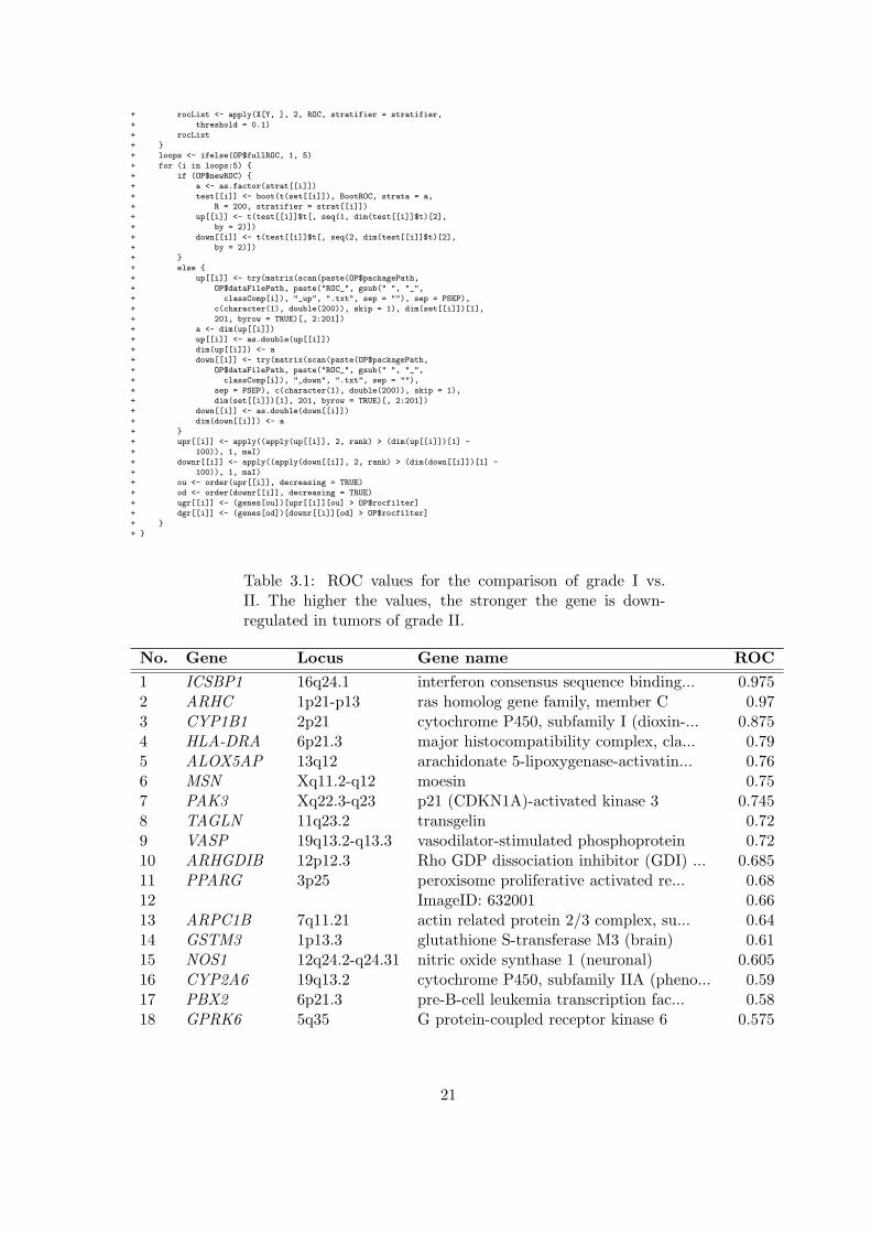
Table 3.1: ROC values for the comparison of grade I vs.II. The higher the values, the stronger the gene is down-regulated in tumors of grade II.
No. Gene Locus Gene name ROC
1 ICSBP1 16q24.1 interferon consensus sequence binding... 0.9752 ARHC 1p21-p13 ras homolog gene family, member C 0.973 CYP1B1 2p21 cytochrome P450, subfamily I (dioxin-... 0.8754 HLA-DRA 6p21.3 major histocompatibility complex, cla... 0.795 ALOX5AP 13q12 arachidonate 5-lipoxygenase-activatin... 0.766 MSN Xq11.2-q12 moesin 0.757 PAK3 Xq22.3-q23 p21 (CDKN1A)-activated kinase 3 0.7458 TAGLN 11q23.2 transgelin 0.729 VASP 19q13.2-q13.3 vasodilator-stimulated phosphoprotein 0.7210 ARHGDIB 12p12.3 Rho GDP dissociation inhibitor (GDI) ... 0.68511 PPARG 3p25 peroxisome proliferative activated re... 0.6812 ImageID: 632001 0.6613 ARPC1B 7q11.21 actin related protein 2/3 complex, su... 0.6414 GSTM3 1p13.3 glutathione S-transferase M3 (brain) 0.6115 NOS1 12q24.2-q24.31 nitric oxide synthase 1 (neuronal) 0.60516 CYP2A6 19q13.2 cytochrome P450, subfamily IIA (pheno... 0.5917 PBX2 6p21.3 pre-B-cell leukemia transcription fac... 0.5818 GPRK6 5q35 G protein-coupled receptor kinase 6 0.575
21

No. Gene Locus Gene name ROC
19 GADD45B 19p13.3 growth arrest and DNA-damage-inducibl... 0.56520 HLA-DRA 6p21.3 major histocompatibility complex, cla... 0.55521 SERPING1 11q12-q13.1 serine (or cysteine) proteinase inhib... 0.55522 HOXB2 17q21-q22 homeo box B2 0.5523 TAF2J ImageID: 786125 0.5524 NOS2A 17q11.2-q12 nitric oxide synthase 2A (inducible, ... 0.54525 TCF15 20p13 transcription factor 15 (basic helix-... 0.54526 FGF18 5q34 fibroblast growth factor 18 0.5427 ARF4L 17q12-q21 ADP-ribosylation factor 4-like 0.5428 ARHB 2pter-p12 ras homolog gene family, member B 0.5429 DAXX 6p21.3 death-associated protein 6 0.53530 LRP8 1p34 low density lipoprotein receptor-rela... 0.5331 TIMP3 22q12.3 tissue inhibitor of metalloproteinase... 0.51532 UMP-CMPK UMP-CMP kinase 0.5133 CHC1 1p36.1 chromosome condensation 1 0.5134 SERPINH2 11q13.5 serine (or cysteine) proteinase inhib... 0.50535 PRKACB 1p36.1 protein kinase, cAMP-dependent, catal... 0.49536 Gene: DKE 0.4937 TNXB 6p21.3 tenascin XB 0.4938 LTBP2 14q24 latent transforming growth factor bet... 0.4639 PTK2 8q24-qter PTK2 protein tyrosine kinase 2 0.4640 HSPA1A 6p21.3 heat shock 70kD protein 1A 0.4441 LILRA2 19q13.4 leukocyte immunoglobulin-like recepto... 0.4342 NOV 8q24.1 nephroblastoma overexpressed gene 0.42543 CCNG2 4q13.3 cyclin G2 0.41544 EFEMP1 2p16 EGF-containing fibulin-like extracell... 0.41545 GNB2 7q22 guanine nucleotide binding protein (G... 0.4146 LTBP1 2p22-p21 latent transforming growth factor bet... 0.405
Table 3.2: ROC values for the comparison of grade I vs. II.The higher the values, the stronger the gene is up-regulatedin tumors of grade II.
No. Gene Locus Gene name ROC
1 ImageID: 42156 0.672 GSPT1 16p13.1 G1 to S phase transition 1 0.633 ImageID: 726311 0.6154 E2F6 22q11 E2F transcription factor 6 0.595 TC10 2p21 likely ortholog of mouse TC10-alpha 0.576 TTK 6q13-q21 TTK protein kinase 0.5657 HSD17B4 5q21 hydroxysteroid (17-beta) dehydrogenas... 0.568 TCEB1L 5q31 transcription elongation factor B (SI... 0.5559 CKS2 9q22 CDC28 protein kinase 2 0.55
22

No. Locus Gene Gene name ROC
10 LDHB 12p12.2-p12.1 lactate dehydrogenase B 0.54511 GJA4 1p35.1 gap junction protein, alpha 4, 37kD (... 0.48512 E2F3 6p22 E2F transcription factor 3 0.4813 E4F1 16p13.3 E4F transcription factor 1 0.47514 TOP2B 3p24 topoisomerase (DNA) II beta (180kD) 0.46515 ImageID: 77723 0.45516 CCNA1 13q12.3-q13 cyclin A1 0.44517 CRP 1q21-q23 C-reactive protein, pentraxin-related 0.44518 TEAD4 12p13.2-p13.3 TEA domain family member 4 0.4419 RAD52 12p13-p12.2 RAD52 homolog (S. cerevisiae) 0.4420 AK3 1 adenylate kinase 3 0.41521 NEK2 1q32.2-q41 NIMA (never in mitosis gene a)-relate... 0.41
Table 3.3: ROC values for the comparison of grade I vs.III. The higher the values, the stronger the gene is down-regulated in tumors of grade III.
No. Gene Locus Gene name ROC
1 CDK7 5q12.1 cyclin-dependent kinase 7 (MO15 homol... 0.9952 PTPN18 2q21.3 protein tyrosine phosphatase, non-rec... 0.9753 PTPRF 1p34 protein tyrosine phosphatase, recepto... 0.954 HABP2 10q26.11 hyaluronan binding protein 2 0.8755 BRCA2 13q12.3 breast cancer 2, early onset 0.8656 COL11A1 1p21 collagen, type XI, alpha 1 0.8557 CCNH 5q13.3-q14 cyclin H 0.8558 GCP3 13q34 spindle pole body protein 0.839 TNFRSF12 1p36.2 tumor necrosis factor receptor superf... 0.7910 CAMK1 3p25.2 calcium/calmodulin-dependent protein ... 0.78511 DCTD 4q35.1 dCMP deaminase 0.77512 UMP-CMPK UMP-CMP kinase 0.76513 HLA-DRA 6p21.3 major histocompatibility complex, cla... 0.76514 ITGAL 16p11.2 integrin, alpha L (antigen CD11A (p18... 0.7515 GLG1 16q22-q23 golgi apparatus protein 1 0.7516 RAGE 14q32 renal tumor antigen 0.7417 LILRA2 19q13.4 leukocyte immunoglobulin-like recepto... 0.7318 GNA15 19p13.3 guanine nucleotide binding protein (G... 0.7319 CDKN2C 1p32 cyclin-dependent kinase inhibitor 2C ... 0.72520 IL1B 2q14 interleukin 1, beta 0.6821 VASP 19q13.2-q13.3 vasodilator-stimulated phosphoprotein 0.66522 EFEMP1 2p16 EGF-containing fibulin-like extracell... 0.65523 CDH3 16q22.1 cadherin 3, type 1, P-cadherin (place... 0.64524 BCL2A1 15q24.3 BCL2-related protein A1 0.62525 PPARG 3p25 peroxisome proliferative activated re... 0.615
23

No. Gene Locus Gene name ROC
26 FGF12B 3 fibroblast growth factor 12B 0.60527 PBX1 1q23 pre-B-cell leukemia transcription fac... 0.59528 BUB1B 15q15 BUB1 budding uninhibited by benzimida... 0.5829 GSTM2 1p13.3 glutathione S-transferase M2 (muscle) 0.56530 MSX1 4p16.3-p16.1 msh homeo box homolog 1 (Drosophila) 0.56531 MAP1B 5q13 microtubule-associated protein 1B 0.5632 ImageID: 546631 0.55533 GABRA5 15q11.2-q12 gamma-aminobutyric acid (GABA) A rece... 0.5434 AKT1 14q32.32 v-akt murine thymoma viral oncogene h... 0.53535 MEOX1 17q21 mesenchyme homeo box 1 0.5236 NOS1 12q24.2-q24.31 nitric oxide synthase 1 (neuronal) 0.5137 PDGFRL 8p22-p21.3 platelet-derived growth factor recept... 0.5138 MAT2A 2p11.2 methionine adenosyltransferase II, al... 0.539 LTBP2 14q24 latent transforming growth factor bet... 0.46540 NRAS 1p13.2 neuroblastoma RAS viral (v-ras) oncog... 0.43541 AP3B1 5q13.2 adaptor-related protein complex 3, be... 0.43542 MGST2 4q28-q31 microsomal glutathione S-transferase 2 0.4343 PBX2 6p21.3 pre-B-cell leukemia transcription fac... 0.4344 RBBP7 Xp22.31 retinoblastoma binding protein 7 0.4345 SELPLG 12q24 selectin P ligand 0.4346 NFKB1 4q24 nuclear factor of kappa light polypep... 0.42547 CAPG 2cen-q24 capping protein (actin filament), gel... 0.42548 IFI16 1q22 interferon, gamma-inducible protein 16 0.4249 NEDD8 14q11.2 neural precursor cell expressed, deve... 0.41550 TOP3A 17p12-17p11.2 topoisomerase (DNA) III alpha 0.4151 LTBP2 14q24 latent transforming growth factor bet... 0.40552 RAB31 18p11.3 RAB31, member RAS oncogene family 0.40553 RRP22 22q12.2 RAS-related on chromosome 22 0.405
Table 3.4: ROC values for the comparison of grade I vs. III.The higher the values, the stronger the gene is up-regulatedin tumors of grade III.
No. Gene Locus Gene name ROC
1 IGFBP3 7p13-p12 insulin-like growth factor binding pr... 0.9952 AKT3 1q43-q44 v-akt murine thymoma viral oncogene h... 0.9953 CKS2 9q22 CDC28 protein kinase 2 0.984 CKS2 9q22 CDC28 protein kinase 2 0.7955 KLRB1 12p13 killer cell lectin-like receptor subf... 0.7756 CENPF 1q32-q41 centromere protein F (350/400kD, mito... 0.737 LDHB 12p12.2-p12.1 lactate dehydrogenase B 0.7258 CDH1 16q22.1 cadherin 1, type 1, E-cadherin (epith... 0.79 GADD45A 1p31.2-p31.1 growth arrest and DNA-damage-inducibl... 0.655
24

No. Locus Gene Gene name ROC
10 CTNNB1 3p21 catenin (cadherin-associated protein)... 0.64511 CDK5R1 17q11.2 cyclin-dependent kinase 5, regulatory... 0.62512 ARHGDIA 17q25.3 Rho GDP dissociation inhibitor (GDI) ... 0.6213 TUBA2 13q11 tubulin, alpha 2 0.61514 ImageID: 345227 0.5915 CDKN2D 19p13 cyclin-dependent kinase inhibitor 2D ... 0.5816 ImageID: 298459 0.5717 GNAS1 ImageID: 629176 0.56518 PLAG1 8q12 pleiomorphic adenoma gene 1 0.5519 EP300 22q13.2 E1A binding protein p300 0.5420 CD4 12pter-p12 CD4 antigen (p55) 0.5421 G22P1 22q13.2-q13.31 thyroid autoantigen 70kD (Ku antigen) 0.53522 RAD9 11q13.1-q13.2 RAD9 homolog (S. pombe) 0.5323 TCP1 6q25-q27 t-complex 1 0.52524 CCND1 11q13 cyclin D1 (PRAD1: parathyroid adenoma... 0.52525 SDCCAG1 14q22 serologically defined colon cancer an... 0.526 HK1 10q22 hexokinase 1 0.49527 CSTB 21q22.3 cystatin B (stefin B) 0.49528 CDKN2D 19p13 cyclin-dependent kinase inhibitor 2D ... 0.4829 E4F1 16p13.3 E4F transcription factor 1 0.4830 CHRM3 1q41-q44 cholinergic receptor, muscarinic 3 0.46531 SOX9 17q24.3-q25.1 SRY (sex determining region Y)-box 9 ... 0.46532 SCD 10q23-q24 stearoyl-CoA desaturase (delta-9-desa... 0.45533 HMGIY 6p21 high-mobility group (nonhistone chrom... 0.4534 CFL1 11q13 cofilin 1 (non-muscle) 0.44535 PSMB1 6q27 proteasome (prosome, macropain) subun... 0.4436 CCT2 12q13.2 chaperonin containing TCP1, subunit 2... 0.4437 RYR2 1q42.1-q43 ryanodine receptor 2 (cardiac) 0.43538 LILRB5 19q13.4 leukocyte immunoglobulin-like recepto... 0.42539 PPM1D 17q23.1 protein phosphatase 1D magnesium-depe... 0.42540 TRAP1 16p12.3 heat shock protein 75 0.42541 STK15 20q13.2-q13.3 serine/threonine kinase 15 0.42542 PAK3 Xq22.3-q23 p21 (CDKN1A)-activated kinase 3 0.42543 PPP2R5B 11q12 protein phosphatase 2, regulatory sub... 0.4244 PCK2 14q11.2 phosphoenolpyruvate carboxykinase 2 (... 0.41545 RAGA 9p21.2 Ras-related GTP-binding protein 0.41546 CYP3A5 7q21.1 cytochrome P450, subfamily IIIA (niph... 0.4147 CDK4 12q14 cyclin-dependent kinase 4 0.405
25

Table 3.5: ROC values for the comparison of grade II vs.III. The higher the values, the stronger the gene is down-regulated in tumors of grade III.
No. Gene Locus Gene name ROC
1 GSTM3 1p13.3 glutathione S-transferase M3 (brain) 0.992 TTK 6q13-q21 TTK protein kinase 0.923 MNAT1 14q23 menage a trois 1 (CAK assembly factor) 0.8654 CDC45L 22q11.21 CDC45 cell division cycle 45-like (S.... 0.7955 ImageID: 546631 0.7856 MAP1B 5q13 microtubule-associated protein 1B 0.777 APLP2 11q24 amyloid beta (A4) precursor-like prot... 0.7658 CDKN2C 1p32 cyclin-dependent kinase inhibitor 2C ... 0.7459 CTNNB1 3p21 catenin (cadherin-associated protein)... 0.7410 BCL2A1 15q24.3 BCL2-related protein A1 0.72511 HXB 9q33 hexabrachion (tenascin C, cytotactin) 0.72512 LDHC 11p15.5-p15.3 lactate dehydrogenase C 0.71513 MEOX1 17q21 mesenchyme homeo box 1 0.70514 ST5 11p15 suppression of tumorigenicity 5 0.67515 ImageID: 1007181 0.67516 KNSL1 10q24.1 kinesin-like 1 0.6517 SYNCOILIN 1p34.3-p33 intermediate filament protein syncoilin 0.6518 E2F1 20q11.2 E2F transcription factor 1 0.64519 MSX1 4p16.3-p16.1 msh homeo box homolog 1 (Drosophila) 0.64520 PRLR 5p14-p13 prolactin receptor 0.63521 RB1 13q14.2 retinoblastoma 1 (including osteosarc... 0.63522 PLCD1 3p22-p21.3 phospholipase C, delta 1 0.6223 CCNA1 13q12.3-q13 cyclin A1 0.58524 ImageID: 365392 0.5625 CCNK 14q32 cyclin K 0.5626 DLEU1 13q14.3 deleted in lymphocytic leukemia, 1 0.5627 HSD17B4 5q21 hydroxysteroid (17-beta) dehydrogenas... 0.5528 TNFRSF12 1p36.2 tumor necrosis factor receptor superf... 0.52529 RAB31 18p11.3 RAB31, member RAS oncogene family 0.5130 BRCA2 13q12.3 breast cancer 2, early onset 0.5131 HOXA4 7p15-p14 homeo box A4 0.5132 CCNH 5q13.3-q14 cyclin H 0.4933 PDHB 3p21.1-p14.2 pyruvate dehydrogenase (lipoamide) beta 0.4934 NEK2 1q32.2-q41 NIMA (never in mitosis gene a)-relate... 0.4935 FGF9 13q11-q12 fibroblast growth factor 9 (glia-acti... 0.47536 FDX1 11q22 ferredoxin 1 0.47537 HABP2 10q26.11 hyaluronan binding protein 2 0.4738 LIPC 15q21-q23 lipase, hepatic 0.4739 TOP3A 17p12-17p11.2 topoisomerase (DNA) III alpha 0.4640 PRKCQ 10p15 protein kinase C, theta 0.4641 RAGE 14q32 renal tumor antigen 0.45542 TNFRSF10C 8p22-p21 tumor necrosis factor receptor superf... 0.45
26

No. Gene Locus Gene name ROC
43 OCLN 5q13.1 occludin 0.44544 FLJ20517 20q13.33 hypothetical protein FLJ20517 0.4445 CHRM1 11q13 cholinergic receptor, muscarinic 1 0.4446 GCP3 13q34 spindle pole body protein 0.4447 NEK2 1q32.2-q41 NIMA (never in mitosis gene a)-relate... 0.43548 MAD1L1 7p22 MAD1 mitotic arrest deficient-like 1 ... 0.43549 MGST2 4q28-q31 microsomal glutathione S-transferase 2 0.42550 ZNF187 6p22 zinc finger protein 187 0.42551 ST13 22q13.2 suppression of tumorigenicity 13 (col... 0.42552 DCTD 4q35.1 dCMP deaminase 0.425
Table 3.6: ROC values for the comparison of grade II vs. III.The higher the values, the stronger the gene is up-regulatedin tumors of grade III.
No. Gene Locus Gene name ROC
1 CYP1B1 2p21 cytochrome P450, subfamily I (dioxin-... 0.9552 CSTB 21q22.3 cystatin B (stefin B) 0.7553 CDKN2D 19p13 cyclin-dependent kinase inhibitor 2D ... 0.7354 CHRM3 1q41-q44 cholinergic receptor, muscarinic 3 0.7155 LBC 15q24-q25 lymphoid blast crisis oncogene 0.696 HOXC11 12q12-q13 homeo box C11 0.677 ALOX12 17p13.1 arachidonate 12-lipoxygenase 0.6658 NOTCH3 19p13.2-p13.1 Notch homolog 3 (Drosophila) 0.629 PYCR1 17q25.3 pyrroline-5-carboxylate reductase 1 0.6110 GRIK1 21q22.11 glutamate receptor, ionotropic, kaina... 0.5911 SDCCAG1 14q22 serologically defined colon cancer an... 0.58512 PAK3 Xq22.3-q23 p21 (CDKN1A)-activated kinase 3 0.57513 EIF2S2 20pter-q12 eukaryotic translation initiation fac... 0.56514 GSTM3 1p13.3 glutathione S-transferase M3 (brain) 0.56515 EGR1 5q31.1 early growth response 1 0.5516 ACTG2 2p13.1 actin, gamma 2, smooth muscle, enteric 0.54517 PCK2 14q11.2 phosphoenolpyruvate carboxykinase 2 (... 0.5418 KATNA1 6q25.1 katanin p60 (ATPase-containing) subun... 0.53519 CCND2 12p13 cyclin D2 0.5320 IGFBP3 7p13-p12 insulin-like growth factor binding pr... 0.5321 GRN 17q21.32 granulin 0.52522 ALDOB 9q21.3-q22.2 aldolase B, fructose-bisphosphate 0.5123 MAD1L1 7p22 MAD1 mitotic arrest deficient-like 1 ... 0.50524 K-ALPHA-1 12q12-12q14.3 tubulin, alpha, ubiquitous 0.4925 EPS8 12q23-q24 epidermal growth factor receptor path... 0.4926 DAXX 6p21.3 death-associated protein 6 0.48527 PCNT2 21q22.3 pericentrin 2 (kendrin) 0.47
27

No. Locus Gene Gene name ROC
28 ACTR1B 2q11.1-q11.2 ARP1 actin-related protein 1 homolog ... 0.4729 TPM4 19p13.1 tropomyosin 4 0.4630 MBL2 10q11.2-q21 mannose-binding lectin (protein C) 2,... 0.4631 DDB1 11q12-q13 damage-specific DNA binding protein 1... 0.4532 ARHGDIA 17q25.3 Rho GDP dissociation inhibitor (GDI) ... 0.44533 CDKN1A 6p21.2 cyclin-dependent kinase inhibitor 1A ... 0.4434 SPG7 16q24.3 spastic paraplegia 7, paraplegin (pur... 0.4435 RYR2 1q42.1-q43 ryanodine receptor 2 (cardiac) 0.43536 APOA2 1q21-q23 apolipoprotein A-II 0.43537 MST1R 3p21.3 macrophage stimulating 1 receptor (c-... 0.43538 KRT6A 12q12-q13 keratin 6A 0.4339 EDN3 20q13.2-q13.3 endothelin 3 0.4340 TIMP1 Xp11.3-p11.23 tissue inhibitor of metalloproteinase... 0.42541 MLL2 12q12-q14 myeloid/lymphoid or mixed-lineage leu... 0.42542 TIMP3 22q12.3 tissue inhibitor of metalloproteinase... 0.4243 CHST3 10q22.3 carbohydrate (chondroitin 6) sulfotra... 0.41544 ARPC1B 7q11.21 actin related protein 2/3 complex, su... 0.41545 COL7A1 3p21.1 collagen, type VII, alpha 1 (epidermo... 0.4146 ARHC 1p21-p13 ras homolog gene family, member C 0.41
Table 3.7: ROC values for the comparison of grade I andII vs. III. The higher the values, the stronger the gene isdown-regulated in tumors of grade III.
No. Gene Locus Gene name ROC
1 IGFBP3 7p13-p12 insulin-like growth factor binding pr... 0.8952 CHRM3 1q41-q44 cholinergic receptor, muscarinic 3 0.813 ARHGDIA 17q25.3 Rho GDP dissociation inhibitor (GDI) ... 0.764 PCK2 14q11.2 phosphoenolpyruvate carboxykinase 2 (... 0.7155 CSTB 21q22.3 cystatin B (stefin B) 0.716 CDKN2D 19p13 cyclin-dependent kinase inhibitor 2D ... 0.6857 MAD1L1 7p22 MAD1 mitotic arrest deficient-like 1 ... 0.628 SDCCAG1 14q22 serologically defined colon cancer an... 0.619 CKS2 9q22 CDC28 protein kinase 2 0.610 LBC 15q24-q25 lymphoid blast crisis oncogene 0.58511 PHB 17q21 prohibitin 0.5712 TCEB2 16p12.3 transcription elongation factor B (SI... 0.5713 ARHGDIA 17q25.3 Rho GDP dissociation inhibitor (GDI) ... 0.5614 AKT3 1q43-q44 v-akt murine thymoma viral oncogene h... 0.54515 MST1R 3p21.3 macrophage stimulating 1 receptor (c-... 0.5416 NMOR2 ImageID: 324217 0.53517 TUBA2 13q11 tubulin, alpha 2 0.53518 PFN1 17p13.3 profilin 1 0.53
28

No. Gene Locus Gene name ROC
19 CDKN2A 9p21 cyclin-dependent kinase inhibitor 2A ... 0.52520 TFAP2A 6p24 transcription factor AP-2 alpha (acti... 0.5221 PAK3 Xq22.3-q23 p21 (CDKN1A)-activated kinase 3 0.51522 CDK5R1 17q11.2 cyclin-dependent kinase 5, regulatory... 0.49523 ACTG2 2p13.1 actin, gamma 2, smooth muscle, enteric 0.49524 UBE2I 16p13.3 ubiquitin-conjugating enzyme E2I (UBC... 0.48525 GNAS1 ImageID: 629176 0.48526 ImageID: 23172 0.47527 SNL 7p22 singed-like (fascin homolog, sea urch... 0.4628 GRN 17q21.32 granulin 0.45529 ARHGAP1 Rho GTPase activating protein 1 0.43530 ALOX12 17p13.1 arachidonate 12-lipoxygenase 0.43531 EGR1 5q31.1 early growth response 1 0.4232 DLK1 14q32 delta-like 1 homolog (Drosophila) 0.4233 RYR2 1q42.1-q43 ryanodine receptor 2 (cardiac) 0.41534 CTNNB1 3p21 catenin (cadherin-associated protein)... 0.4135 DDB1 11q12-q13 damage-specific DNA binding protein 1... 0.4136 HOXC11 12q12-q13 homeo box C11 0.4137 PDGFB 22q13.1 platelet-derived growth factor beta p... 0.40538 PSG4 19q13.2 pregnancy specific beta-1-glycoprotei... 0.40539 PLAUR 19q13 plasminogen activator, urokinase rece... 0.405
Table 3.8: ROC values for the comparison of grade I andII vs. III. The higher the values, the stronger the gene isup-regulated in tumors of grade III.
No. Gene Locus Gene name ROC
1 CDK7 5q12.1 cyclin-dependent kinase 7 (MO15 homol... 0.9552 CDKN2C 1p32 cyclin-dependent kinase inhibitor 2C ... 0.913 BRCA2 13q12.3 breast cancer 2, early onset 0.9054 GCP3 13q34 spindle pole body protein 0.885 TTK 6q13-q21 TTK protein kinase 0.886 ImageID: 546631 0.8757 BCL2A1 15q24.3 BCL2-related protein A1 0.8658 CCNH 5q13.3-q14 cyclin H 0.8559 MAP1B 5q13 microtubule-associated protein 1B 0.8510 UMP-CMPK UMP-CMP kinase 0.8411 MEOX1 17q21 mesenchyme homeo box 1 0.8412 HABP2 10q26.11 hyaluronan binding protein 2 0.8113 TNFRSF12 1p36.2 tumor necrosis factor receptor superf... 0.814 LDHC 11p15.5-p15.3 lactate dehydrogenase C 0.78515 GSTM3 1p13.3 glutathione S-transferase M3 (brain) 0.7716 DCTD 4q35.1 dCMP deaminase 0.765
29

No. Locus Gene Gene name ROC
17 MSX1 4p16.3-p16.1 msh homeo box homolog 1 (Drosophila) 0.7318 RAGE 14q32 renal tumor antigen 0.67519 IL1B 2q14 interleukin 1, beta 0.6620 PBX1 1q23 pre-B-cell leukemia transcription fac... 0.65521 APLP2 11q24 amyloid beta (A4) precursor-like prot... 0.65522 PRLR 5p14-p13 prolactin receptor 0.62523 CCNK 14q32 cyclin K 0.62524 PTPN18 2q21.3 protein tyrosine phosphatase, non-rec... 0.61525 CTNNB1 3p21 catenin (cadherin-associated protein)... 0.626 PLCD1 3p22-p21.3 phospholipase C, delta 1 0.59527 GNA15 19p13.3 guanine nucleotide binding protein (G... 0.5928 CDC45L 22q11.21 CDC45 cell division cycle 45-like (S.... 0.5929 DLEU1 13q14.3 deleted in lymphocytic leukemia, 1 0.5930 COL11A1 1p21 collagen, type XI, alpha 1 0.56531 TOP3A 17p12-17p11.2 topoisomerase (DNA) III alpha 0.55532 LTBP2 14q24 latent transforming growth factor bet... 0.5433 MGST2 4q28-q31 microsomal glutathione S-transferase 2 0.53534 MNAT1 14q23 menage a trois 1 (CAK assembly factor) 0.52535 ImageID: 365392 0.51536 GABRA5 15q11.2-q12 gamma-aminobutyric acid (GABA) A rece... 0.51537 RBBP7 Xp22.31 retinoblastoma binding protein 7 0.5138 OCLN 5q13.1 occludin 0.4939 SYNCOILIN 1p34.3-p33 intermediate filament protein syncoilin 0.4940 RAB31 18p11.3 RAB31, member RAS oncogene family 0.47541 ImageID: 110764 0.4742 ST5 11p15 suppression of tumorigenicity 5 0.46543 LIPC 15q21-q23 lipase, hepatic 0.4644 PDGFRL 8p22-p21.3 platelet-derived growth factor recept... 0.43545 ZNF187 6p22 zinc finger protein 187 0.4346 CAMK1 3p25.2 calcium/calmodulin-dependent protein ... 0.42547 FLJ20517 20q13.33 hypothetical protein FLJ20517 0.4148 NEK2 1q32.2-q41 NIMA (never in mitosis gene a)-relate... 0.405
Table 3.9: ROC values for the comparison of grade I vs. IIand III. The higher the values, the stronger the gene is down-regulated in tumors of grade II and III.
No. Gene Locus Gene name ROC
1 VASP 19q13.2-q13.3 vasodilator-stimulated phosphoprotein 0.892 HLA-DRA 6p21.3 major histocompatibility complex, cla... 0.883 ICSBP1 16q24.1 interferon consensus sequence binding... 0.814 ALOX5AP 13q12 arachidonate 5-lipoxygenase-activatin... 0.795 NOS1 12q24.2-q24.31 nitric oxide synthase 1 (neuronal) 0.79
30

No. Gene Locus Gene name ROC
6 PPARG 3p25 peroxisome proliferative activated re... 0.7757 PBX2 6p21.3 pre-B-cell leukemia transcription fac... 0.778 ARHC 1p21-p13 ras homolog gene family, member C 0.739 UMP-CMPK UMP-CMP kinase 0.7110 HOXB2 17q21-q22 homeo box B2 0.70511 CHC1 1p36.1 chromosome condensation 1 0.6512 FGF12B 3 fibroblast growth factor 12B 0.64513 LTBP2 14q24 latent transforming growth factor bet... 0.6214 LILRA2 19q13.4 leukocyte immunoglobulin-like recepto... 0.60515 CCNG2 4q13.3 cyclin G2 0.60516 HLA-DRA 6p21.3 major histocompatibility complex, cla... 0.60517 TAGLN 11q23.2 transgelin 0.618 GPRK6 5q35 G protein-coupled receptor kinase 6 0.58519 CDKN2C 1p32 cyclin-dependent kinase inhibitor 2C ... 0.5520 CYP2A6 19q13.2 cytochrome P450, subfamily IIA (pheno... 0.5521 GAPCENA 9q34.11 rab6 GTPase activating protein (GAP a... 0.5422 SELPLG 12q24 selectin P ligand 0.53523 CYP1B1 2p21 cytochrome P450, subfamily I (dioxin-... 0.53524 CASP8 2q33-q34 caspase 8, apoptosis-related cysteine... 0.5325 PTPRF 1p34 protein tyrosine phosphatase, recepto... 0.5326 ImageID: 632001 0.49527 EFEMP1 2p16 EGF-containing fibulin-like extracell... 0.4928 ARHG 11p15.5-p15.4 ras homolog gene family, member G (rh... 0.4929 ARHB 2pter-p12 ras homolog gene family, member B 0.48530 STAT2 12q12 signal transducer and activator of tr... 0.4831 TAF2J ImageID: 786125 0.4832 NEDD8 14q11.2 neural precursor cell expressed, deve... 0.4733 GADD45B 19p13.3 growth arrest and DNA-damage-inducibl... 0.4734 ELF3 1q32.2 E74-like factor 3 (ets domain transcr... 0.4735 LRP8 1p34 low density lipoprotein receptor-rela... 0.4636 CDC25B 20p13 cell division cycle 25B 0.4637 SERPINH2 11q13.5 serine (or cysteine) proteinase inhib... 0.4638 MAP3K11 11q13.1-q13.3 mitogen-activated protein kinase kina... 0.45539 TCF15 20p13 transcription factor 15 (basic helix-... 0.4440 MMP14 14q11-q12 matrix metalloproteinase 14 (membrane... 0.43541 COL5A1 9q34.2-q34.3 collagen, type V, alpha 1 0.4342 F10 13q34 coagulation factor X 0.42543 HSPA1A 6p21.3 heat shock 70kD protein 1A 0.4244 ALDOB 9q21.3-q22.2 aldolase B, fructose-bisphosphate 0.4245 CUL4A 13q34 cullin 4A 0.41546 EN2 7q36 engrailed homolog 2 0.40547 PTK2 8q24-qter PTK2 protein tyrosine kinase 2 0.405
31

Table 3.10: ROC values for the comparison of grade I vs.II and III. The higher the values, the stronger the gene isup-regulated in tumors of grade II and III.
No. Gene Locus Gene name ROC
1 CKS2 9q22 CDC28 protein kinase 2 0.752 CKS2 9q22 CDC28 protein kinase 2 0.7353 IGFBP3 7p13-p12 insulin-like growth factor binding pr... 0.714 AKT3 1q43-q44 v-akt murine thymoma viral oncogene h... 0.685 TEAD4 12p13.2-p13.3 TEA domain family member 4 0.6156 E4F1 16p13.3 E4F transcription factor 1 0.6057 STK15 20q13.2-q13.3 serine/threonine kinase 15 0.68 CDK5R1 17q11.2 cyclin-dependent kinase 5, regulatory... 0.599 LILRB5 19q13.4 leukocyte immunoglobulin-like recepto... 0.56510 E2F6 22q11 E2F transcription factor 6 0.5511 CYP3A5 7q21.1 cytochrome P450, subfamily IIIA (niph... 0.53512 SOX9 17q24.3-q25.1 SRY (sex determining region Y)-box 9 ... 0.52513 ImageID: 77723 0.52514 RAD52 12p13-p12.2 RAD52 homolog (S. cerevisiae) 0.5215 TFPI2 7q22 tissue factor pathway inhibitor 2 0.5116 PLAG1 8q12 pleiomorphic adenoma gene 1 0.517 HINT 5q31.2 histidine triad nucleotide binding pr... 0.4918 ImageID: 42156 0.4719 CCT2 12q13.2 chaperonin containing TCP1, subunit 2... 0.4720 CENPF 1q32-q41 centromere protein F (350/400kD, mito... 0.46521 EP300 22q13.2 E1A binding protein p300 0.46522 PER2 2q37.3 period homolog 2 (Drosophila) 0.46523 FBL 19q13.1 fibrillarin 0.4624 TC10 2p21 likely ortholog of mouse TC10-alpha 0.4625 TUBA2 13q11 tubulin, alpha 2 0.4626 GADD45A 1p31.2-p31.1 growth arrest and DNA-damage-inducibl... 0.4527 CDK4 12q14 cyclin-dependent kinase 4 0.4528 STK12 17p13.1 serine/threonine kinase 12 0.4529 PCNA 20pter-p12 proliferating cell nuclear antigen 0.4430 PLAGL1 6q24-q25 pleiomorphic adenoma gene-like 1 0.43531 CTCF 16q21-q22.3 CCCTC-binding factor (zinc finger pro... 0.4332 HCS 7p21.2 cytochrome c 0.4233 GJA4 1p35.1 gap junction protein, alpha 4, 37kD (... 0.41534 GSPT1 16p13.1 G1 to S phase transition 1 0.41535 CYP4A11 1p33 cytochrome P450, subfamily IVA, polyp... 0.4136 ImageID: 340477 0.4137 HMGIY 6p21 high-mobility group (nonhistone chrom... 0.405
Further analysis will only focus on Table 3.9 and 3.10. The comparison of the benigntumor group (grade I, n = 13) to the more aggressive types (grade II and III, n = 17)
32

provides two larger groups, thus increasing the stability of gene selection.
3.4 EASE Analysis
The resulting tables (3.9, 3.10) were submitted to EASE analysis of the GO terms associatedto the selected genes. Given a list of genes with given GO terms the tool EASE allows toidentify a significant overrepresentation of single GO terms in this list with respect to theselection of genes present on the whole chip.
While there are no enrichments of GO terms with a low score in the list of downregulatedgenes (data not shown), the list of upregulated genes contains a number of proliferation as-sociated genes (Table 3.11) with a rather low EASE score, suggesting statistical significance(as a rather recent method it remains to be shown that the scoring used here is a validand stable method). Of special interest is the “Biological Process” branch consisting of thefollowing succession of members, ordered according to their hierarchy in the GO tree:
biological process
physiological processes
cell growth and/or maintenance (18)
cell proliferation (14)
cell cycle (13)
mitotic cell cycle (7)
G1/S transition of mitotic cell cycle (4)
regulation of cell cycle (9)
The number of genes associated with each of the terms are given in parentheses for thoseterms that were identified as being significantly overrepresented in the EASE analysis. Thetree branches once after the term “cell cycle” with 7, respectively 9, genes being associatedwith the term “mitotic cell cycle” and/or “regulation of cell cycle”.
Both other branches of GO, “Cellular Component” and “Molecular Function”, show nosuch sequence of enriched terms. The“Molecular Function”branch is still interesting becauseof the transcription factors that hint at the factors influencing the transcriptional programmof the higher tumor grades.
33

4 IGF Pathway
4.1 ROC analysis
ROC analysis (Table 3.10) identifies the genes IGFBP3 and AKT3 as being upregulatedin tumors of higher grade. Both genes are involved in the signal transduction of growthcontrol mediated by IGF1 or IGF2. IGFBP3 and AKT3 are also included in the centroidsgenerated by shrunken centroid analysis (Figure 3.4). The distribution of expression valuesamong the three tumor grades is presented in Figures 4.1 and 4.2.
It is known that the IGF pathway plays a role in meningioma pathogenesis[Khandwala et al., 2000, Zumkeller & Westphal, 2001], but so far mainly IGF2 expressionhas been associated with higher meningioma tumor grades [Nordqvist & Mathiesen, 2002].IGF2 is not directly identified in the ROC statistic, but as shown in Figure 4.3, a tendencyfor upregulation in atypical and anaplastic tumors is visible. The subsequent t-test verifiesthat this difference is significant (p=0.046) for the upregulation of IGF2 expression fromgrade I to grade III.
> y <- exprs(dataset)[grep("IGF2", as.character(as.vector(maInfo(genes)[,
+ 4]))), ]
> t.test(split(y, WHO)[[1]], split(y, WHO)[[3]], "less")
Welch Two Sample t-test
data: split(y, WHO)[[1]] and split(y, WHO)[[3]]
t = -1.9082, df = 8.049, p-value = 0.04629
alternative hypothesis: true difference in means is less than 0
95 percent confidence interval:
-Inf -0.02636243
sample estimates:
mean of x mean of y
-0.2205929 0.7842787
Upregulation of IGF2 gene expression has been connected with an activated IGFpathway resulting in stronger proliferation for a variety of different tumor types[Khandwala et al., 2000]. The effects are mediated through either the RAS-RAF-MAPKor PI3K-PKB/AKT pathway [Werner & Roberts, 2003]. While the upregulation of IGF2probably presents one way to accelerated growth in meningiomas, our data suggest thatthere might be a second mechanism involving the same pathway, yet different genes. Highexpression of IGFBP3 might result in a similar activation of the IGF-signalling cascade.While to our knowledge no study did explicitely test the expression of this gene in menin-gioma samples to date, it has been one among many genes reported to be upregulated intumors of grade II and III as compared to tumors of grade I by another expression profilingstudy [Watson et al., 2002] on meningiomas.
IGFBP3 strongly binds IGF1 and IGF2 [Furstenberger & Senn, 2002], on the one handremoving IGFs from intercellular space, on the other hand delivering IGFs to cells. Sev-eral diverse actions for IGFBP3 (as protein alone as well as in relation to IGFs) have beendiscussed but not all its effects can be readily explained yet. As free protein without its
34

System Gene Cat-egory
ListHits
ListAll
Pop.Hits
Pop.All
EASEscore
Genes
Biological Pro-cess
cell cycle 13 29 198 1074 0.002 STK12, STK15, EP300,E2F6, CTCF, PLAGL1,CENPF, PCNA,GADD45A, CKS2,RAD52, CDK5R1, CDK4
Biological Pro-cess
cell prolifera-tion
14 29 245 1074 0.004 E4F1, STK12, STK15,EP300, E2F6, CTCF,PLAGL1, CENPF,PCNA, GADD45A,RAD52, CKS2, CDK5R1,FBL
Biological Pro-cess
cell growthand/or mainte-nance
18 29 401 1074 0.009 E4F1, STK12, STK15,EP300, GJA4, TUBA2,E2F6, CTCF, PLAGL1,CENPF, IGFBP3, PCNA,GADD45A, CKS2,RAD52, CDK5R1, CDK4,FBL
Biological Pro-cess
regulation ofcell cycle
9 29 138 1074 0.020 E2F6, CTCF, PLAGL1,CENPF, PCNA,GADD45A, CKS2,CDK5R1, CDK4
Cellular Com-ponent
nucleus 12 20 292 880 0.022 SOX9, STK15, EP300,E2F6, CTCF, HINT,CENPF, GADD45A,RAD52, CDK5R1,PLAGL1, FBL
MolecularFunction
cyclin-dependentprotein kinaseactivity
3 27 12 1057 0.033 CKS2, CDK5R1, CDK4
Biological Pro-cess
mitotic cell cy-cle
7 29 101 1074 0.041 STK15, CENPF, PCNA,GADD45A, CKS2,CDK5R1, CDK4
Biological Pro-cess
G1/S transi-tion of mitoticcell cycle
4 29 33 1074 0.051 GADD45A, CKS2,CDK5R1, CDK4
MolecularFunction
transcriptionco-repressoractivity
3 27 16 1057 0.057 E4F1, E2F6, CTCF
MolecularFunction
transcriptioncofactoractivity
4 27 40 1057 0.071 E4F1, E2F6, CTCF,EP300
Table 3.11: EASE analysis of genes identified as being upregulated in meningiomas of highergrade. The table provides the counts for each GO term for the list provided(ROC analysis) as well as the whole population (Pop., genes on the chip) andthe corresponding EASE score.
35

MN
27M
N30
MN
41M
N45
MN
58M
N2
MN
7M
N10
MN
12M
N36
MN
15M
N37
MN
19M
N10
9M
N40
MN
69M
N42
MN
62M
N47
MN
56B
MN
4M
N14
MN
16M
N20
MN
22M
N11
9M
N11
3M
N63
BM
N34
MN
67
ln(e
xpre
ssio
n ra
tio)
−1.0
−0.5
0.0
0.5
1.0
1.5
2.0
IGFBP3
WHO grade IWHO grade IIWHO grade III
Figure 4.1: Distribution of IGFBP3 expression values over the three different tumor grades.
MN
27M
N30
MN
41M
N45
MN
58M
N2
MN
7M
N10
MN
12M
N36
MN
15M
N37
MN
19M
N10
9M
N40
MN
69M
N42
MN
62M
N47
MN
56B
MN
4M
N14
MN
16M
N20
MN
22M
N11
9M
N11
3M
N63
BM
N34
MN
67
ln(e
xpre
ssio
n ra
tio)
−1.0
−0.5
0.0
0.5
1.0
1.5
2.0
AKT3
WHO grade IWHO grade IIWHO grade III
Figure 4.2: Distribution of AKT3 expression values over the three different tumor grades.
36

MN
27M
N30
MN
41M
N45
MN
58M
N2
MN
7M
N10
MN
12M
N36
MN
15M
N37
MN
19M
N10
9M
N40
MN
69M
N42
MN
62M
N47
MN
56B
MN
4M
N14
MN
16M
N20
MN
22M
N11
9M
N11
3M
N63
BM
N34
MN
67
ln(e
xpre
ssio
n ra
tio)
−3
−2
−1
0
1
2
3
4
IGF2
WHO grade IWHO grade IIWHO grade III
Grade I Grade II Grade III
−2
−1
01
23
Expression ratios for each tumor grade
ln(e
xpre
ssio
n ra
tio)
WHO grade IWHO grade IIWHO grade III
Figure 4.3: Distribution of IGF2 expression values over the three different tumor grades.Details of the boxplot are given in Figure 2.1.
●
●
●
●
●
●
●
● ●
●
●
●
●
●
●●
●
●
●
●
●
●
●
●
●
●●
●
●
−1.
0
−0.
5
0.0
0.5
1.0
1.5
−0.5
0.0
0.5
1.0
ln(Ratio) for IGFBP3 / AKT3 Correlation of expression = 0.91
IGFBP3
AK
T3
WHO grade IWHO grade IIWHO grade III
Figure 4.4: Correlation of expression values for gene IGFBP3 and AKT3. Tumor grade iscoded in color as given by the legend.
37

usual cargo of IGFs it seems to enhance cell apoptosis [Butt & Williams, 2001]. But ithas also been shown that IGFBP3 can bind to the cell surface when having bound IGF[Conover, 1992]. Once bound to the cell surface, the protein is degraded partially, thusreleasing IGF. It is hypothesized, that this leads to a locally increased IGF concentration,stimulating proliferation of the cells. This positive effect on cell growth has been demon-strated on bovine fibroblasts. Interestingly it was shown that this effect of increased prolif-eration is mediated by the PI3-K and AKT pathway [Conover et al., 2000], which suggeststhat the upregulated AKT3 gene further enhances activation of the IGF pathway.
Both genes share a rather high correlation, but since the signalling cascade relies onphosphorylation it is not obvious how the expressions of both genes are synchronized to thisextent.
4.2 Correlated genes
To identify whether there are further genes involved that are related to the IGFpathway, a search for genes significantly correlated whith the gene IGFBP3 is beingconducted using the ”genefinder” algorithm provided by the bioconductor framework[Project Bioconductor, 2000]. This algorithm allows identification of genes with similarexpression patterns using different distance measurements. In this case correlation was usedto define similarity. The 12 genes with highest correlation are given in Table 4.1, while thesame number of genes with highest inverse correlation are given in Table 4.2.
> corGenes <- findGenes("358862", "correlation", X = 12, V = "none",
+ W = rep(1, 30))
> antiCorGenes <- findGenes("358862", "correlation", X = 12, V = "none",
+ W = rep(-1, 30))
While some of the listed genes might be interesting for further study, the known func-tional aspects of these genes as well as the strength of correlation do not provide a stronglink to the IGF pathway.
4.3 Patients with upregulated IGF pathway
Looking at Figure 4.4, it would be interesting to see if the patients can be split into subgroupsin correlation with CGH data. Therefore, the AKT3 expression values are being extracted.
> X <- "360838"
> a <- grep(X, as.character(maInfo(genes)$ImageID))
> akt3 <- as.double(as.vector(exprs(dataset[a, ])))
These data are subsequently analyzed in conjunction with the CGH and LOH data bydecision tree analysis. The resolution of CGH analysis had to be lowered to full chromosomesfor this. “dim14” thus represents a loss that occurred anywhere on chromosome 14, while“enh17” signifies a gain of material anywhere on chromosome 17. The analysis aimed atidentifying a set of factors among the CGH or LOH data that could be used to determinethe expression status.
> CGH <- maInfo(patients)[, 15:60]
> CGH <- as.data.frame(ifelse(CGH == "-" | CGH == "RET", "0", "1"))
> tree(akt3 ~ ., cbind(akt3, CGH))
38

No. Gene Locus Gene name Corr.
1 AKT3 1q43-q44 v-akt murine thymoma viral oncogene h... 0.912 CDH1 16q22.1 cadherin 1, type 1, E-cadherin (epith... 0.663 TXN 9q31 thioredoxin 0.564 CDKN2D 19p13 cyclin-dependent kinase inhibitor 2D ... 0.565 CSTB 21q22.3 cystatin B (stefin B) 0.556 ARHGDIA 17q25.3 Rho GDP dissociation inhibitor (GDI) ... 0.527 ARF1 1q42 ADP-ribosylation factor 1 0.528 TNFAIP3 6q23.1-q25.3 tumor necrosis factor, alpha-induced ... 0.529 YWHAZ 8q23.1 tyrosine 3-monooxygenase/tryptophan 5... 0.4910 ALDOA 16q22-q24 aldolase A, fructose-bisphosphate 0.4911 WEE1 11p15.3-p15.1 WEE1+ homolog (S. pombe) 0.4912 RANBP1 22q11.21 RAN binding protein 1 0.49
Table 4.1: Genes positively correlated with the expression of IGFBP3.
No. Gene Locus Gene name Corr.
1 HLA-DRA 6p21.3 major histocompatibility complex, cla... 0.592 PTPN18 2q21.3 protein tyrosine phosphatase, non-rec... 0.583 HCLS1 3q13 hematopoietic cell-specific Lyn subst... 0.574 SELPLG 12q24 selectin P ligand 0.575 RAGE 14q32 renal tumor antigen 0.576 CDH3 16q22.1 cadherin 3, type 1, P-cadherin (place... 0.567 IL1B 2q14 interleukin 1, beta 0.558 GSTM2 1p13.3 glutathione S-transferase M2 (muscle) 0.559 PDGFRB 5q31-q32 platelet-derived growth factor recept... 0.5510 TCF19 6p21.3 transcription factor 19 (SC1) 0.5511 KRAS2 12p12.1 v-Ki-ras2 Kirsten rat sarcoma 2 viral... 0.5512 MMP3 11q22.3 matrix metalloproteinase 3 (stromelys... 0.54
Table 4.2: Genes negatively correlated with the expression of IGFBP3.
39

node), split, n, deviance, yval
* denotes terminal node
1) root 26 4.6730 0.05574
2) dim10: 0 18 0.6328 -0.17320
4) dim22: 0 9 0.2443 -0.11640 *
5) dim22: 1 9 0.3304 -0.23000 *
3) dim10: 1 8 0.9748 0.57080 *
> LOH <- maInfo(patients)[, 10:14]
> LOH <- as.data.frame(ifelse(LOH == "-" | LOH == "RET", "0", "1"))
> tree(akt3 ~ ., cbind(akt3, LOH))
node), split, n, deviance, yval
* denotes terminal node
1) root 17 2.4030 0.02513
2) LOH10q: 0 12 0.5183 -0.16520
4) LOH22q: 0 6 0.2184 -0.09203 *
5) LOH22q: 1 6 0.2357 -0.23840 *
3) LOH10q: 1 5 0.4071 0.48190 *
From the result it is obvious that a good partitioning of the expression data of AKT3can be realized on basis of the loss of chromosome 10. This is visualized in Figure 4.5.The left diagramm shows the combined expression of genes IGFBP3 and AKT3 with theshape representing the status of chromosome 10. Triangles represent samples with no lossof genomic material on chromosome 10, squares denotes a loss and patients with missingCGH data are omitted. The difference in AKT3 expression between the two classes is alsorepresented in the right part of the figure as a boxplot.
If the loss of chromosome 10 has an influence on the molecular state of the cell, it wouldbe interesting to see whether the expression data can be used to classify the two groups onbasis of the status of chromosome 10. Again, shrunken centroid is used to investigate thisclassification.
A threshold of 1.9 is chosen to determine the genes of the centroid, the class probabilitiesand the confusion while cross validating.
> Chr10 <- cbind(as.character(as.vector(maInfo(patients)[["ID-No."]])),
+ as.character(as.vector(CGH$dim10)), akt3)
> mData3 <- pamr.knnimpute(list(x = exprs(dataset)[, !is.na(Chr10[,
+ 2])], y = as.factor(ifelse(Chr10[!is.na(Chr10[, 2]), 2] ==
+ "1", "Dim Chr.10", "No loss"))))
> mData3$genenames <- as.character(maInfo(genes)[, 4])
> mData3$location <- as.character(maInfo(genes)[, 6])
> mData3$genenames[mData3$genenames == ""] <- paste("ImageID:",
+ as.character(maInfo(genes)[mData3$genenames == "", 7]))
> mData3$samplelabels <- colnames(mData3$x)
> train3 <- pamr.train(mData3)
> cv3 <- pamr.cv(train3, mData3, folds = balanced.folds(train3$y,
+ nfold = 19))
> t3 <- 1.9
> pamr.confusion(cv3, t3)
Dim Chr.10 No loss Class Error rate
Dim Chr.10 7 1 0.1250000
No loss 2 17 0.1052632
Overall error rate= 0.11
The classification (Figures 4.6, 4.7, 4.8) shows a low amount of misclassified samplesand, as expected, both IGFBP3 and AKT3 are good predictors for the loss of chromosome10. Without making any assumptions about cause and effect it can still be said that thereis a strong relation on the molecular level between the loss of this chromosome and theexpression pattern measured. This relation is significantly stronger than the relation betweenpathological classification and the expression status of the samples.
It is intriguing to speculate whether the loss of the gene PTEN is the reason whythe upregulation of AKT3 expression correlates with loss of chromosome 10. This gene
40

is a tumor suppressor gene situated on 10q23.3 and well known to suppress activation(phosphorylation) of AKT [Stambolic et al., 1998]. Thus the loss of expression of PTENmight lead to a weaker repression of AKT and stimulate IGF-controlled proliferation. Butit has also been shown that the gene PTEN seldomly shows mutations in meningiomas[Bostrom et al., 1998, Peters et al., 1998, Joachim et al., 2001].
41

−1.
0
−0.
5
0.0
0.5
1.0
1.5
−0.5
0.0
0.5
1.0
Differentielle Expression für IGFBP3 / AKT3 Korrelation der Expression = 0.91
IGFBP3
AK
T3
Grade I / No LossGrade II / No LossGrade I / Loss on chr.10Grade II / Loss on chr.10Grade III / Loss on chr.10
●
Dim Chr.10 No loss
−0.
50.
00.
51.
0
Expression ratios for AKT3 depending on loss of Chr.10
ln(e
xpre
ssio
n ra
tio)
No lossDim Chr.10
Figure 4.5: Correlation of IGFBP3 and AKT3 expression and loss on chromosome 10. De-tails of the boxplot are given in Figure 2.1.
0 1 2 3
Value of threshold
Mis
clas
sific
atio
n er
ror
2088 1103 450 225 114 55 36 23 14 5 4 3 2 2
Number of genes
0.0
0.2
0.4
0.6
0.8
0 1 2 3
Value of threshold
Mis
clas
sific
atio
n er
ror
2088 1103 450 225 114 55 36 23 14 5 4 3 2 2
Number of genes
0.0
0.4
0.8
Dim Chr.10No loss
Figure 4.6: Misclassification of the shrunken centroid analysis of meningioma samples clas-sified by loss of genomic material on chromosome ten. The minimum lies arounda shrinkage of 1.9.
42

Cross−validated class probabilities
Cro
ss−
valid
ated
pro
babi
litie
s
MN
40M
N62
MN
63B
MN
34M
N4
MN
12M
N67
MN
20M
N27
MN
30M
N41
MN
69M
N42
MN
45M
N47
MN
58M
N56
BM
N2
MN
7M
N10
MN
36M
N14
MN
15M
N16
MN
37M
N19
MN
22
0%20
%40
%60
%80
%10
0%
0%20
%40
%60
%80
%10
0%● ●
●
●
●
●
●
●
●
●
●
●
●●
●
●
●
●
●●
● ●
●
●
● ●
●● ●
●
●
●
●
●
●
●
●
●
●
●●
●
●
●
●
●●
● ●
●
●
● ●
●
Class Dim Chr.10 Class No loss
Figure 4.7: Shrunken centroid analysis of meningioma samples classified by loss of genomicmaterial on chromosome ten. The figure shows the cross validated probabilityfor each sample to belong in one of the two classes according to the calculatedcentroid.
43

Dim Chr.10 No loss
ABCB1
CDKN1A
ENO2
FTL
IDH2
CAP2
FKBP2
ALDOA
CTNNB1
MDM4
CDK5R1
ALDOA
ImageID: 345227
CD4
TMSB10
ATF1
CDH1
ImageID: 901596
ImageID: 965544
MDM4
EP300
GAMT
ENC1
AKT3
CENPF
LDHB
IGFBP3
(7q21.1)
(6p21.2)
(12p13)
(19q13.3−q13.4)
(15q26.1)
(6p22.2)
(11q13.1−q13.3)
(16q22−q24)
(3p21)
(1q32)
(17q11.2)
(16q22−q24)
(12pter−p12)
(2p11.2)
(12q13)
(16q22.1)
(1q32)
(22q13.2)
(19p13.3)
(5q12−q13.3)
(1q43−q44)
(1q32−q41)
(12p12.2−p12.1)
(7p13−p12)
Figure 4.8: Shrunken centroid analysis of meningioma samples classified by loss of genomicmaterial on chromosome ten. The figure shows the resulting centroid.
44

5 WNT-signalling pathway
5.1 ROC analysis
ROC analysis (Table 3.10) also identifies the gene CDK5R1 (p35 ) as being upregulatedin tumors of higher grade. This gene is also included in the shrunken centroid given inFigure 3.4. The gene is interesting because the set of genes correlating with its expressionyields a strong hint at a second pathway that might play an important role in meningiomapathogenesis.
> corGenes2 <- findGenes("796579", "correlation", X = 15, V = "none",
+ W = rep(1, 30))
> antiCorGenes2 <- findGenes("796579", "correlation", X = 15, V = "none",
+ W = rep(-1, 30))
The 15 genes with highest correlation of expression to CDK5R1 are given in Table5.1 while the 15 genes with highest inverse correlation are given in Table 5.2. CDK5R1is known to interact with CDK5, leading to a variety of effects [Smith & Tsai, 2002]including the dissociation of CTNNB1 (β-catenin) from cadherins [Kwon et al., 2000].Since CTNNB1 stabilizes cadherin mediated cell-cell adhesion, upregulation of CDK5R1might indicate a reduction of such interactions in meningiomas of a higher grade[Kwon et al., 2000]. But the primary effect is probably resulting from the dissociatedcytoplasmic CTNNB1 [Ben-Ze’ev et al., 2000], a protein that is a central component ofthe WNT-signalling pathway and has been identified as a tumor promoting gene inseveral other tumor types [Brabletz et al., 2002, Howng et al., 2002], especially colorec-tal cancer [Bright-Thomas & Hargest, 2003]. Free CTNNB1 translocates to the nucleus,binds different types of transcription factors, and functions as transcriptional enhancerin these complexes. Another transcription factor less related to CTNNB1 but knownto enhance the transcriptional activation of the EP300 paralogue CBP [Giles et al., 1998,Shimomura et al., 1996], ATF1 is also found to be correlated to CDK5R1 expression. As-suming that the upregulation of these genes leads to a strong enhancement in expression ofCTNNB1 regulated genes, it is certainly not surprising to find two genes well known to becontrolled by CTNNB1, ENC1 [Fujita et al., 2001] and CCND1 [Shtutman et al., 1999] inthe table, too.
Taken together these data present evidence for an upregulation of transcription ofCTNNB1/ATF1 controlled genes in more aggressive meningiomas.
> corGenes2ImageID <- findGenesImageID("796579", "correlation",
+ X = 15, V = "none", W = rep(1, 30))
> interestingGenes <- corGenes2ImageID[c(1, 3, 5, 6, 11, 14, 15),
+ 1]
> expIG <- NULL
> for (i in 1:length(interestingGenes)) expIG <- rbind(expIG, singleGene(interestingGenes[i]))
> colnames(expIG) <- colnames(exprs(dataset))
> rownames(expIG) <- corGenes2[c(1, 3, 5, 6, 11, 14, 15), 1]
> scaled <- t(scale(t(as.matrix(expIG))))
> sortedN <- colnames(scaled)[order(apply(scaled, 2, mean, na.rm = TRUE))]
> sortedC <- c("black", "yellow", "white")[match(WHO[order(apply(scaled,
45

+ 2, mean, na.rm = TRUE))], c("I", "II", "III"))]
> sortedB <- c("gray", "black", "black")[match(WHO[order(apply(scaled,
+ 2, mean, na.rm = TRUE))], c("I", "II", "III"))]
> sortedD <- split(t(scaled[, order(apply(scaled, 2, mean, na.rm = TRUE))]),
+ seq(1, 30))
> sortedC14 <- c("black", "white")[as.integer(CGH$dim14[order(apply(scaled,
+ 2, mean, na.rm = TRUE))])]
> sortedC1 <- c("black", "white")[as.integer(CGH$dim1[order(apply(scaled,
+ 2, mean, na.rm = TRUE))])]
> sortedC141 <- c("black", "gray", "yellow", "white")[(as.integer(CGH$dim14[order(apply(scaled,
+ 2, mean, na.rm = TRUE))]) - 1) * 2 + as.integer(CGH$dim1[order(apply(scaled,
+ 2, mean, na.rm = TRUE))])]
> sortedB14 <- c("gray", "black")[as.integer(CGH$dim14[order(apply(scaled,
+ 2, mean, na.rm = TRUE))])]
> sortedB1 <- c("gray", "black")[as.integer(CGH$dim1[order(apply(scaled,
+ 2, mean, na.rm = TRUE))])]
> sortedB141 <- c("gray", "gray", "black", "black")[(as.integer(CGH$dim14[order(apply(scaled,
+ 2, mean, na.rm = TRUE))]) - 1) * 2 + as.integer(CGH$dim1[order(apply(scaled,
+ 2, mean, na.rm = TRUE))])]
The upregulation of these genes is also presented in Figure 5.1. Here the expressionvalues for all genes were scaled genewise and presented in a joined form as a boxplot. Thesamples are sorted according to the mean over six genes (MDM4, CTNNB1, CCND1, ENC1,ATF1, EP300 ) four of which are mentioned above (MDM4 and EP300 were included heresince there existed hints at a functional relation to the WNT-pathway which were laterconsidered to be too weak). The expression values have been scaled genewise. It can beseen from the color coding, that there is a prevalence of higher tumor grades in the stronglyupregulated samples.
More importantly the strength of upregulation can be correlated with the CGH statusof the samples. Again decision tree analysis is used to find a corresponding cytogeneticaberration.
> meanV <- apply(scaled, 2, mean, na.rm = TRUE)
> tree(meanV ~ ., cbind(meanV, CGH))
node), split, n, deviance, yval
* denotes terminal node
1) root 27 22.590 -0.0619
2) dim14: 0 16 10.140 -0.5403
4) dim1: 0 11 4.554 -0.6299 *
5) dim1: 1 5 5.301 -0.3430 *
3) dim14: 1 11 3.461 0.6339 *
In this case the loss of chromosome 14 seems to be the major factor determining expres-sion of these genes. The boxplot of the scaled expression values is reproduced with a variedcolor coding expressing the loss of chromosomal material in Figure 5.2, 5.3, and 5.4.
5.2 Shrunken centroid
If the loss of chromosome 14 has an impact on the expression of such a set of genes, shrunkencentroid analysis should again be able to classify the samples according to this criterium. Athreshold of 1.5 seems optimal for separation of the classes.
> Chr14 <- cbind(as.character(as.vector(maInfo(patients)[["ID-No."]])),
+ as.character(as.vector(CGH$dim14)), akt3)
> mData4 <- pamr.knnimpute(list(x = exprs(dataset)[, !is.na(Chr14[,
+ 2])], y = as.factor(ifelse(Chr14[!is.na(Chr14[, 2]), 2] ==
+ "1", "Dim Chr.14", "No loss"))))
> mData4$genenames <- as.character(maInfo(genes)[, 4])
> mData4$location <- as.character(maInfo(genes)[, 6])
> mData4$genenames[mData4$genenames == ""] <- paste("ImageID:",
+ as.character(maInfo(genes)[mData4$genenames == "", 7]))
> mData4$samplelabels <- colnames(mData4$x)
> train4 <- pamr.train(mData4)
> cv4 <- pamr.cv(train4, mData4, folds = balanced.folds(train3$y,
+ nfold = 19))
> t4 <- 1.5
46

No. Gene Locus Gene name ROC
1 MDM4 1q32 Mdm4, transformed 3T3 cell double min... 0.832 CENPF 1q32-q41 centromere protein F (350/400kD, mito... 0.823 CTNNB1 3p21 catenin (cadherin-associated protein)... 0.84 GAMT 19p13.3 guanidinoacetate N-methyltransferase 0.785 CCND1 11q13 cyclin D1 (PRAD1: parathyroid adenoma... 0.776 ENC1 5q12-q13.3 ectodermal-neural cortex (with BTB-li... 0.767 LDHB 12p12.2-p12.1 lactate dehydrogenase B 0.768 ImageID: 965544 0.769 FTL 19q13.3-q13.4 ferritin, light polypeptide 0.7510 PCK2 14q11.2 phosphoenolpyruvate carboxykinase 2 (... 0.7411 MDM4 1q32 Mdm4, transformed 3T3 cell double min... 0.7312 IDH2 15q26.1 isocitrate dehydrogenase 2 (NADP+), m... 0.7313 ImageID: 901596 0.7314 ATF1 12q13 activating transcription factor 1 0.7115 EP300 22q13.2 E1A binding protein p300 0.68
Table 5.1: Genes positively correlated with the expression of CDK5R1.
> pamr.confusion(cv4, t4)
Dim Chr.14 No loss Class Error rate
Dim Chr.14 9 2 0.1818182
No loss 4 12 0.2500000
Overall error rate= 0.219
The results are depicted in Figure 5.7. All genes that were discussed also appear inthe centroid. Again, the relation between loss of this chromosome to the measured expres-sion values seems to be stronger than the link between pathological classification of thetumors and the molecular state of the samples. The loss of chromosome 14 is known to af-fect meningioma pathogenesis [Cai et al., 2001] though its effects have not yet been clearlyidentified.
47

No. Gene Locus Gene name ROC
1 HP 16q22.1 haptoglobin 0.792 FLJ20517 20q13.33 hypothetical protein FLJ20517 0.793 PPP2R5E 14q23.1 protein phosphatase 2, regulatory sub... 0.794 SERPINF2 17p13 serine (or cysteine) proteinase inhib... 0.775 HPGD 4q34-q35 hydroxyprostaglandin dehydrogenase 15... 0.776 PSPH 7p15.2-p15.1 phosphoserine phosphatase 0.777 CKS2 9q22 CDC28 protein kinase 2 0.778 E2F6 22q11 E2F transcription factor 6 0.769 CHRM1 11q13 cholinergic receptor, muscarinic 1 0.7510 RANBP1 22q11.21 RAN binding protein 1 0.7511 ZNF146 19q13.1 zinc finger protein 146 0.7512 SSRP1 11q12 structure specific recognition protei... 0.7413 CYP2A6 19q13.2 cytochrome P450, subfamily IIA (pheno... 0.7414 LIF 22q12.2 leukemia inhibitory factor (cholinerg... 0.7415 PRKAR1A 17q23-q24 protein kinase, cAMP-dependent, regul... 0.74
Table 5.2: Genes negatively correlated with the expression of CDK5R1.
48

●
●
●
●
●
●
MN
2M
N36
MN
14M
N16
MN
22M
N42
MN
10M
N58
MN
19M
N37
MN
45M
N27
MN
4M
N47
MN
7M
N67
MN
30M
N12
MN
41M
N69
MN
109
MN
119
MN
56B
MN
113
MN
34M
N63
BM
N15
MN
62M
N20
MN
40
−3
−2
−1
0
1
2
Expression of WNT pathway related genes
WHO grade IWHO grade IIWHO grade III
Figure 5.1: Scaled expression of the selected, WNT pathway related genes (MDM4,CTNNB1, CCND1, ENC1, ATF1, EP300 ), sorted for their median and col-ored according to tumor grade. Details of the boxplot are given in Figure 2.1.
●
●
●
●
●
●
MN
2M
N36
MN
14M
N16
MN
22M
N42
MN
10M
N58
MN
19M
N37
MN
45M
N27
MN
4M
N47
MN
7M
N67
MN
30M
N12
MN
41M
N69
MN
109
MN
119
MN
56B
MN
113
MN
34M
N63
BM
N15
MN
62M
N20
MN
40
−3
−2
−1
0
1
2
Expression of WNT pathway related genes
No lossLoss on chr. 10
Figure 5.2: Scaled expression of the selected, Wnt-pathway related genes (MDM4, CTNNB1,CCND1, ENC1, ATF1, EP300 ), sorted for their median and colored accordingto loss of chromosome 14. Details of the boxplot are given in Figure 2.1.
49

●
●
●
●
●
●
MN
2M
N36
MN
14M
N16
MN
22M
N42
MN
10M
N58
MN
19M
N37
MN
45M
N27
MN
4M
N47
MN
7M
N67
MN
30M
N12
MN
41M
N69
MN
109
MN
119
MN
56B
MN
113
MN
34M
N63
BM
N15
MN
62M
N20
MN
40
−3
−2
−1
0
1
2
Expression of WNT pathway related genes
No lossLoss on chr. 10
Figure 5.3: Scaled expression of the selected, Wnt-pathway related genes (MDM4, CTNNB1,CCND1, ENC1, ATF1, EP300 ), sorted for their median and colored accordingto loss of chromosome 1. Details of the boxplot are given in Figure 2.1.
●
●
●
●
●
●
MN
2M
N36
MN
14M
N16
MN
22M
N42
MN
10M
N58
MN
19M
N37
MN
45M
N27
MN
4M
N47
MN
7M
N67
MN
30M
N12
MN
41M
N69
MN
109
MN
119
MN
56B
MN
113
MN
34M
N63
BM
N15
MN
62M
N20
MN
40
−3
−2
−1
0
1
2
Expression of WNT pathway related genes
No lossLoss on chr. 1Loss on chr. 14Loss on chr.1 and chr.14
Figure 5.4: Scaled expression of the selected, Wnt-pathway related genes (MDM4, CTNNB1,CCND1, ENC1, ATF1, EP300 ), sorted for their median and colored accordingto loss of chromosomes 1 and 14. Details of the boxplot are given in Figure 2.1.
50

0.0 0.5 1.0 1.5 2.0 2.5 3.0
Value of threshold
Mis
clas
sific
atio
n er
ror
2088 1242 606 338 175 97 62 38 20 15 13 7 3 1
Number of genes
0.0
0.2
0.4
0.6
0.8
0.0 0.5 1.0 1.5 2.0 2.5 3.0
Value of threshold
Mis
clas
sific
atio
n er
ror
2088 1242 606 338 175 97 62 38 20 15 13 7 3 1
Number of genes
0.0
0.4
0.8
Dim Chr.14No loss
Figure 5.5: Misclassification of the shrunken centroid analysis of meningioma samples clas-sified by loss of genomic material on chromosome forteen.
51
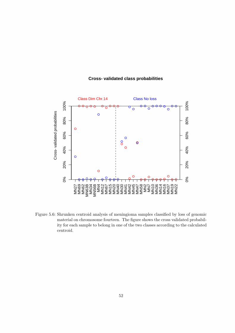
Cross−validated class probabilities
Cro
ss−
valid
ated
pro
babi
litie
s
MN
27M
N69
MN
62M
N63
BM
N34
MN
56B
MN
4M
N12
MN
67M
N15
MN
20M
N40
MN
30M
N41
MN
42M
N45
MN
47M
N58
MN
2M
N7
MN
10M
N36
MN
14M
N16
MN
37M
N19
MN
22
0%20
%40
%60
%80
%10
0%
0%20
%40
%60
%80
%10
0%
●
● ● ● ● ●
●
●●
● ● ●
●
●
●●
●
● ●●
● ● ● ●●
● ●
●
● ● ● ● ●
●
●●
● ● ●
●
●
●●
●
● ●●
● ● ● ●●
● ●
Class Dim Chr.14 Class No loss
Figure 5.6: Shrunken centroid analysis of meningioma samples classified by loss of genomicmaterial on chromosome fourteen. The figure shows the cross validated probabil-ity for each sample to belong in one of the two classes according to the calculatedcentroid.
52
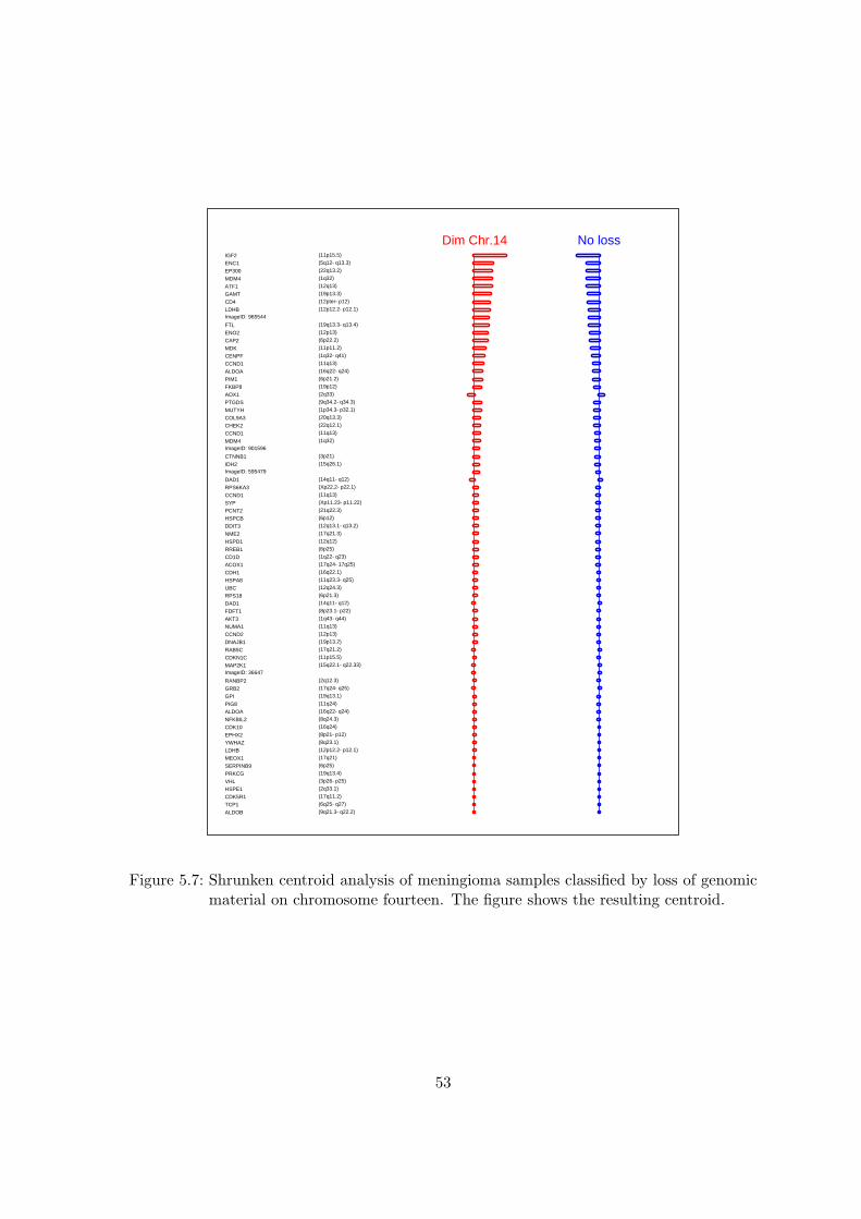
Dim Chr.14 No loss
ALDOBTCP1CDK5R1HSPE1VHLPRKCGSERPINB9MEOX1LDHBYWHAZEPHX2CDK10NFKBIL2ALDOAPIG8GPIGRB2RANBP2
ImageID: 36647MAP2K1CDKN1CRAB5C
DNAJB1CCND2
NUMA1AKT3FDFT1DAD1RPS18UBCHSPA8CDH1ACOX1CD1DRREB1HSPD1NME2
DDIT3HSPCBPCNT2SYPCCND1RPS6KA3DAD1
ImageID: 595479IDH2CTNNB1
ImageID: 901596MDM4CCND1CHEK2COL9A3
MUTYHPTGDSAOX1
FKBP8PIM1ALDOACCND1CENPFMDKCAP2ENO2FTL
ImageID: 965544LDHBCD4GAMTATF1MDM4
EP300ENC1IGF2
(9q21.3−q22.2)(6q25−q27)(17q11.2)(2q33.1)(3p26−p25)(19q13.4)(6p25)(17q21)(12p12.2−p12.1)(8q23.1)(8p21−p12)(16q24)(8q24.3)(16q22−q24)(11q24)(19q13.1)(17q24−q25)(2q12.3)
(15q22.1−q22.33)(11p15.5)(17q21.2)(19p13.2)(12p13)(11q13)(1q43−q44)(8p23.1−p22)(14q11−q12)(6p21.3)(12q24.3)(11q23.3−q25)(16q22.1)(17q24−17q25)(1q22−q23)(6p25)(12q12)(17q21.3)(12q13.1−q13.2)(6p12)(21q22.3)(Xp11.23−p11.22)(11q13)(Xp22.2−p22.1)(14q11−q12)
(15q26.1)(3p21)
(1q32)(11q13)(22q12.1)(20q13.3)(1p34.3−p32.1)(9q34.2−q34.3)(2q33)(19p12)(6p21.2)(16q22−q24)(11q13)(1q32−q41)(11p11.2)(6p22.2)(12p13)(19q13.3−q13.4)
(12p12.2−p12.1)(12pter−p12)(19p13.3)(12q13)(1q32)(22q13.2)(5q12−q13.3)(11p15.5)
Figure 5.7: Shrunken centroid analysis of meningioma samples classified by loss of genomicmaterial on chromosome fourteen. The figure shows the resulting centroid.
53

6 Additional Analyses
6.1 Real-Time-Quantitative-PCR (RQ-PCR)
Microarray expression data of several genes were verified using RQ-PCR. For each of thesegenes the correlation between microarray and real-time data were checked. Since the real-time dataset comprised of more patients this data was used to depict the correlations ofexpression with regard to WHO grade and loss of chromosome 10 or 14 for each of the genesanalyzed. All data are summarized in the tables following the graphics (Table 6.1 and 6.2).
> mgrep <- function(X, Y) {
+ A <- NULL
+ for (i in X) A <- c(A, grep(i, Y))
+ A
+ }
> geneNo <- 10
> taqMan <- read.delim(paste(OP$packagePath, OP$dataFilePath, OP$rqdata,
+ sep = PSEP))[, c(1:4, 6:(geneNo + 5))]
> uArray <- t(exprs(dataset)[mgrep(c("IGF2", "MDM4", "AKT3", "IGFBP3",
+ "CENPF", "CDK5R1", "VASP", "PTPRF", "ELF3"), as.character(as.vector(maInfo(genes)[,
+ 4])))[c(1, 3, 4, 5, 6, 8, 10, 11, 12)], ])
> link <- match(taqMan[, 1], rownames(uArray))
> joined <- cbind(log(taqMan[, 2:(dim(taqMan)[2] - 4)]), uArray[link,
+ ], taqMan[, (dim(taqMan)[2] - 3):dim(taqMan)[2]])
> rownames(joined) <- taqMan[, 1]
> colnames(joined) <- c(paste("RT", colnames(taqMan)[2:(dim(taqMan)[2] -
+ 4)], sep = "-"), paste("uA", colnames(uArray), sep = "-"),
+ "WHO", "DIM1", "DIM10", "DIM14")
54

MN
2M
N7
MN
10M
N12
MN
15M
N19
MN
27M
N36
MN
45M
N58
MN
30M
N37
MN
41M
N69
MN
4M
N14
MN
16M
N20
MN
22M
N40
MN
42M
N47
MN
62M
N56
BM
N10
9M
N67
MN
34M
N63
BM
N11
9M
N11
3
Comparison Real−Time/Microarray (IGF2)
ln(e
xpre
ssio
n ra
tio)
−3
−2
−1
0
1
2
RT / WHO grade IuArray / WHO grade IRT / WHO grade IIuArray / WHO grade IIRT / WHO grade IIIuArray / WHO grade III
●
●
●
●
●
●
●
●
●
●
●
●
●
●
●
●
●
●
●
●
●
●
●
●
●
●
●
●
●
●
−2 −1 0 1
−2
−1
01
2
Comparison Real−Time/Microarray (IGF2) correlation = 0.663020015693884
ln(expression ratio) − Real Time
ln(e
xpre
ssio
n ra
tio)
− M
icro
arra
y
MN
2M
N7
MN
10M
N12
MN
15M
N17
MN
19M
N27
MN
36M
N11
MN
45M
N58
MN
30M
N37
MN
41M
N53
MN
66M
N69
MN
4M
N14
MN
16M
N20
MN
22M
N40
MN
42M
N47
MN
61M
N62
MN
56B
MN
109
MN
67M
N34
MN
49A
MN
63B
MN
64M
N11
9M
N11
3
Real−Time data correlated to WHO grade (IGF2)
ln(e
xpre
ssio
n ra
tio)
−4
−2
0
2
WHO grade IWHO grade IIWHO grade III
MN
2M
N10
MN
15M
N36
MN
11M
N45
MN
58M
N30
MN
37M
N41
MN
53M
N22
MN
42M
N47
MN
64M
N7
MN
12M
N17
MN
19M
N27
MN
66M
N69
MN
4M
N14
MN
16M
N20
MN
40M
N61
MN
62M
N56
BM
N67
MN
34M
N49
AM
N63
BM
N10
9M
N11
9M
N11
3
Real−Time data correlated to Loss on Chr.1 (IGF2)
ln(e
xpre
ssio
n ra
tio)
−4
−2
0
2
No loss on Chr.1Loss on Chr.1Not determined
MN
2M
N7
MN
10M
N15
MN
17M
N19
MN
27M
N36
MN
11M
N45
MN
58M
N30
MN
37M
N41
MN
53M
N66
MN
69M
N14
MN
16M
N22
MN
42M
N47
MN
61M
N56
BM
N4
MN
20M
N62
MN
67M
N49
AM
N64
MN
12M
N40
MN
34M
N63
BM
N10
9M
N11
9M
N11
3
Real−Time data correlated to Loss on Chr.10 (IGF2)
ln(e
xpre
ssio
n ra
tio)
−4
−2
0
2
No loss on Chr.10Loss on Chr.10Not determined
MN
2M
N7
MN
10M
N17
MN
19M
N36
MN
11M
N45
MN
58M
N30
MN
37M
N41
MN
53M
N66
MN
14M
N16
MN
22M
N40
MN
42M
N47
MN
61M
N64
MN
12M
N15
MN
27M
N69
MN
4M
N20
MN
62M
N56
BM
N67
MN
34M
N49
AM
N63
BM
N10
9M
N11
9M
N11
3
Real−Time data correlated to Loss on Chr.14 (IGF2)
ln(e
xpre
ssio
n ra
tio)
−4
−2
0
2
No loss on Chr.14Loss on Chr.14Not determined
Figure 6.1: Real time data for gene IGF2. The upper left plot shows a direct comparisonof microaray and real-time expression data. The upper right plot shows thecorresponding correlation between the measurements. The subsequent threeplots show the real-time expression data sorted and colored according to threedifferent factors: WHO grade (middle left), loss on Chr.10 (middle right) andloss on Chr.14 (bottom). 55

MN
2M
N7
MN
10M
N12
MN
15M
N19
MN
27M
N36
MN
45M
N58
MN
30M
N37
MN
41M
N69
MN
4M
N14
MN
16M
N20
MN
22M
N40
MN
42M
N47
MN
62M
N56
BM
N10
9M
N67
MN
34M
N63
BM
N11
9M
N11
3
Comparison Real−Time/Microarray (MDM4)
ln(e
xpre
ssio
n ra
tio)
−2
−1
0
1
2
RT / WHO grade IuArray / WHO grade IRT / WHO grade IIuArray / WHO grade IIRT / WHO grade IIIuArray / WHO grade III
●
●
●
●
●
●
●
●
●
●
●
●
●
●
●
●
●
●
●
●
●
●
●
●
● ●
●
●
●
●
−1.5 −1.0 −0.5 0.0 0.5 1.0 1.5
−2
−1
01
2
Comparison Real−Time/Microarray (MDM4) correlation = 0.589010760108991
ln(expression ratio) − Real Time
ln(e
xpre
ssio
n ra
tio)
− M
icro
arra
y
MN
2M
N7
MN
10M
N12
MN
15M
N17
MN
19M
N27
MN
36M
N11
MN
45M
N58
MN
30M
N37
MN
41M
N53
MN
66M
N69
MN
4M
N14
MN
16M
N20
MN
22M
N40
MN
42M
N47
MN
61M
N62
MN
56B
MN
109
MN
67M
N34
MN
49A
MN
63B
MN
64M
N11
9M
N11
3
Real−Time data correlated to WHO grade (MDM4)
ln(e
xpre
ssio
n ra
tio)
−1
0
1
2
3
WHO grade IWHO grade IIWHO grade III
MN
2M
N10
MN
15M
N36
MN
11M
N45
MN
58M
N30
MN
37M
N41
MN
53M
N22
MN
42M
N47
MN
64M
N7
MN
12M
N17
MN
19M
N27
MN
66M
N69
MN
4M
N14
MN
16M
N20
MN
40M
N61
MN
62M
N56
BM
N67
MN
34M
N49
AM
N63
BM
N10
9M
N11
9M
N11
3
Real−Time data correlated to Loss on Chr.1 (MDM4)
ln(e
xpre
ssio
n ra
tio)
−1
0
1
2
3
No loss on Chr.1Loss on Chr.1Not determined
MN
2M
N7
MN
10M
N15
MN
17M
N19
MN
27M
N36
MN
11M
N45
MN
58M
N30
MN
37M
N41
MN
53M
N66
MN
69M
N14
MN
16M
N22
MN
42M
N47
MN
61M
N56
BM
N4
MN
20M
N62
MN
67M
N49
AM
N64
MN
12M
N40
MN
34M
N63
BM
N10
9M
N11
9M
N11
3
Real−Time data correlated to Loss on Chr.10 (MDM4)
ln(e
xpre
ssio
n ra
tio)
−1
0
1
2
3
No loss on Chr.10Loss on Chr.10Not determined
MN
2M
N7
MN
10M
N17
MN
19M
N36
MN
11M
N45
MN
58M
N30
MN
37M
N41
MN
53M
N66
MN
14M
N16
MN
22M
N40
MN
42M
N47
MN
61M
N64
MN
12M
N15
MN
27M
N69
MN
4M
N20
MN
62M
N56
BM
N67
MN
34M
N49
AM
N63
BM
N10
9M
N11
9M
N11
3
Real−Time data correlated to Loss on Chr.14 (MDM4)
ln(e
xpre
ssio
n ra
tio)
−1
0
1
2
3
No loss on Chr.14Loss on Chr.14Not determined
Figure 6.2: Real time data for gene MDM4. The upper left plot shows a direct comparisonof microaray and real-time expression data. The upper right plot shows thecorresponding correlation between the measurements. The subsequent threeplots show the real-time expression data sorted and colored according to threedifferent factors: WHO grade (middle left), loss on Chr.10 (middle right) andloss on Chr.14 (bottom). 56

MN
7M
N10
MN
12M
N15
MN
19M
N27
MN
36M
N45
MN
58M
N30
MN
37M
N41
MN
69M
N4
MN
14M
N16
MN
20M
N22
MN
40M
N42
MN
47M
N62
MN
56B
MN
109
MN
67M
N34
MN
63B
MN
119
MN
113
Comparison Real−Time/Microarray (AKT3)
ln(e
xpre
ssio
n ra
tio)
−2
−1
0
1
2
RT / WHO grade IuArray / WHO grade IRT / WHO grade IIuArray / WHO grade IIRT / WHO grade IIIuArray / WHO grade III
●
●
●
●
●●
●
●
●
●
●
●
●
●
●
●
●
●
●
●
●
●
●
●
●
●
●
●
●
−2 −1 0 1 2
−1
01
2
Comparison Real−Time/Microarray (AKT3) correlation = 0.243551022406677
ln(expression ratio) − Real Time
ln(e
xpre
ssio
n ra
tio)
− M
icro
arra
y
MN
2M
N7
MN
10M
N12
MN
15M
N17
MN
19M
N27
MN
36M
N11
MN
45M
N58
MN
30M
N37
MN
41M
N53
MN
66M
N69
MN
4M
N14
MN
16M
N20
MN
22M
N40
MN
42M
N47
MN
61M
N62
MN
56B
MN
109
MN
67M
N34
MN
49A
MN
63B
MN
64M
N11
9M
N11
3
Real−Time data correlated to WHO grade (AKT3)
ln(e
xpre
ssio
n ra
tio)
−3.0
−2.5
−2.0
−1.5
−1.0
−0.5
0.0
WHO grade IWHO grade IIWHO grade III
MN
2M
N10
MN
15M
N36
MN
11M
N45
MN
58M
N30
MN
37M
N41
MN
53M
N22
MN
42M
N47
MN
64M
N7
MN
12M
N17
MN
19M
N27
MN
66M
N69
MN
4M
N14
MN
16M
N20
MN
40M
N61
MN
62M
N56
BM
N67
MN
34M
N49
AM
N63
BM
N10
9M
N11
9M
N11
3
Real−Time data correlated to Loss on Chr.1 (AKT3)
ln(e
xpre
ssio
n ra
tio)
−3.0
−2.5
−2.0
−1.5
−1.0
−0.5
0.0
No loss on Chr.1Loss on Chr.1Not determined
MN
2M
N7
MN
10M
N15
MN
17M
N19
MN
27M
N36
MN
11M
N45
MN
58M
N30
MN
37M
N41
MN
53M
N66
MN
69M
N14
MN
16M
N22
MN
42M
N47
MN
61M
N56
BM
N4
MN
20M
N62
MN
67M
N49
AM
N64
MN
12M
N40
MN
34M
N63
BM
N10
9M
N11
9M
N11
3
Real−Time data correlated to Loss on Chr.10 (AKT3)
ln(e
xpre
ssio
n ra
tio)
−3.0
−2.5
−2.0
−1.5
−1.0
−0.5
0.0
No loss on Chr.10Loss on Chr.10Not determined
MN
2M
N7
MN
10M
N17
MN
19M
N36
MN
11M
N45
MN
58M
N30
MN
37M
N41
MN
53M
N66
MN
14M
N16
MN
22M
N40
MN
42M
N47
MN
61M
N64
MN
12M
N15
MN
27M
N69
MN
4M
N20
MN
62M
N56
BM
N67
MN
34M
N49
AM
N63
BM
N10
9M
N11
9M
N11
3
Real−Time data correlated to Loss on Chr.14 (AKT3)
ln(e
xpre
ssio
n ra
tio)
−3.0
−2.5
−2.0
−1.5
−1.0
−0.5
0.0
No loss on Chr.14Loss on Chr.14Not determined
Figure 6.3: Real time data for gene AKT3. The upper left plot shows a direct comparisonof microaray and real-time expression data. The upper right plot shows thecorresponding correlation between the measurements. The subsequent threeplots show the real-time expression data sorted and colored according to threedifferent factors: WHO grade (middle left), loss on Chr.10 (middle right) andloss on Chr.14 (bottom). 57

MN
2M
N7
MN
10M
N12
MN
15M
N19
MN
27M
N36
MN
45M
N58
MN
30M
N37
MN
41M
N69
MN
4M
N14
MN
16M
N20
MN
22M
N40
MN
42M
N47
MN
62M
N56
BM
N10
9M
N67
MN
34M
N63
BM
N11
9M
N11
3
Comparison Real−Time/Microarray (IGFBP3)
ln(e
xpre
ssio
n ra
tio)
−2
−1
0
1
2
RT / WHO grade IuArray / WHO grade IRT / WHO grade IIuArray / WHO grade IIRT / WHO grade IIIuArray / WHO grade III
●
●
●
●
●
●●●
●
●
●●
● ●
●
●
●
●
●
●
●●
●
●
●
●
●
●
●
●
−1 0 1 2
−1
01
2
Comparison Real−Time/Microarray (IGFBP3) correlation = 0.675306898471307
ln(expression ratio) − Real Time
ln(e
xpre
ssio
n ra
tio)
− M
icro
arra
y
MN
2M
N7
MN
10M
N12
MN
15M
N17
MN
19M
N27
MN
36M
N11
MN
45M
N58
MN
30M
N37
MN
41M
N53
MN
66M
N69
MN
4M
N14
MN
16M
N20
MN
22M
N40
MN
42M
N47
MN
61M
N62
MN
56B
MN
109
MN
67M
N34
MN
49A
MN
63B
MN
64M
N11
9M
N11
3
Real−Time data correlated to WHO grade (IGFBP3)
ln(e
xpre
ssio
n ra
tio)
−6
−4
−2
0
WHO grade IWHO grade IIWHO grade III
MN
2M
N10
MN
15M
N36
MN
11M
N45
MN
58M
N30
MN
37M
N41
MN
53M
N22
MN
42M
N47
MN
64M
N7
MN
12M
N17
MN
19M
N27
MN
66M
N69
MN
4M
N14
MN
16M
N20
MN
40M
N61
MN
62M
N56
BM
N67
MN
34M
N49
AM
N63
BM
N10
9M
N11
9M
N11
3
Real−Time data correlated to Loss on Chr.1 (IGFBP3)
ln(e
xpre
ssio
n ra
tio)
−6
−4
−2
0
No loss on Chr.1Loss on Chr.1Not determined
MN
2M
N7
MN
10M
N15
MN
17M
N19
MN
27M
N36
MN
11M
N45
MN
58M
N30
MN
37M
N41
MN
53M
N66
MN
69M
N14
MN
16M
N22
MN
42M
N47
MN
61M
N56
BM
N4
MN
20M
N62
MN
67M
N49
AM
N64
MN
12M
N40
MN
34M
N63
BM
N10
9M
N11
9M
N11
3
Real−Time data correlated to Loss on Chr.10 (IGFBP3)
ln(e
xpre
ssio
n ra
tio)
−6
−4
−2
0
No loss on Chr.10Loss on Chr.10Not determined
MN
2M
N7
MN
10M
N17
MN
19M
N36
MN
11M
N45
MN
58M
N30
MN
37M
N41
MN
53M
N66
MN
14M
N16
MN
22M
N40
MN
42M
N47
MN
61M
N64
MN
12M
N15
MN
27M
N69
MN
4M
N20
MN
62M
N56
BM
N67
MN
34M
N49
AM
N63
BM
N10
9M
N11
9M
N11
3
Real−Time data correlated to Loss on Chr.14 (IGFBP3)
ln(e
xpre
ssio
n ra
tio)
−6
−4
−2
0
No loss on Chr.14Loss on Chr.14Not determined
Figure 6.4: Real time data for gene IGFBP3. The upper left plot shows a direct comparisonof microaray and real-time expression data. The upper right plot shows thecorresponding correlation between the measurements. The subsequent threeplots show the real-time expression data sorted and colored according to threedifferent factors: WHO grade (middle left), loss on Chr.10 (middle right) andloss on Chr.14 (bottom). 58

MN
2M
N7
MN
10M
N12
MN
15M
N19
MN
27M
N36
MN
45M
N58
MN
30M
N37
MN
41M
N69
MN
4M
N14
MN
16M
N20
MN
22M
N40
MN
42M
N47
MN
62M
N56
BM
N10
9M
N67
MN
34M
N63
BM
N11
9M
N11
3
Comparison Real−Time/Microarray (CENPF)
ln(e
xpre
ssio
n ra
tio)
−3
−2
−1
0
1
2
RT / WHO grade IuArray / WHO grade IRT / WHO grade IIuArray / WHO grade IIRT / WHO grade IIIuArray / WHO grade III
●
●
●
●
●
●●
●
●
●
●
●
●
●●
●
●
●
●
●
●
●
●
●
●
●
●
●
●●
−1.5 −1.0 −0.5 0.0 0.5 1.0 1.5
−2
−1
01
2
Comparison Real−Time/Microarray (CENPF) correlation = 0.527656774092561
ln(expression ratio) − Real Time
ln(e
xpre
ssio
n ra
tio)
− M
icro
arra
y
MN
2M
N7
MN
10M
N12
MN
15M
N17
MN
19M
N27
MN
36M
N11
MN
45M
N58
MN
30M
N37
MN
41M
N53
MN
66M
N69
MN
4M
N14
MN
16M
N20
MN
22M
N40
MN
42M
N47
MN
61M
N62
MN
56B
MN
109
MN
67M
N34
MN
49A
MN
63B
MN
64M
N11
9M
N11
3
Real−Time data correlated to WHO grade (CENPF)
ln(e
xpre
ssio
n ra
tio)
0
2
4
6
WHO grade IWHO grade IIWHO grade III
MN
2M
N10
MN
15M
N36
MN
11M
N45
MN
58M
N30
MN
37M
N41
MN
53M
N22
MN
42M
N47
MN
64M
N7
MN
12M
N17
MN
19M
N27
MN
66M
N69
MN
4M
N14
MN
16M
N20
MN
40M
N61
MN
62M
N56
BM
N67
MN
34M
N49
AM
N63
BM
N10
9M
N11
9M
N11
3
Real−Time data correlated to Loss on Chr.1 (CENPF)
ln(e
xpre
ssio
n ra
tio)
0
2
4
6
No loss on Chr.1Loss on Chr.1Not determined
MN
2M
N7
MN
10M
N15
MN
17M
N19
MN
27M
N36
MN
11M
N45
MN
58M
N30
MN
37M
N41
MN
53M
N66
MN
69M
N14
MN
16M
N22
MN
42M
N47
MN
61M
N56
BM
N4
MN
20M
N62
MN
67M
N49
AM
N64
MN
12M
N40
MN
34M
N63
BM
N10
9M
N11
9M
N11
3
Real−Time data correlated to Loss on Chr.10 (CENPF)
ln(e
xpre
ssio
n ra
tio)
0
2
4
6
No loss on Chr.10Loss on Chr.10Not determined
MN
2M
N7
MN
10M
N17
MN
19M
N36
MN
11M
N45
MN
58M
N30
MN
37M
N41
MN
53M
N66
MN
14M
N16
MN
22M
N40
MN
42M
N47
MN
61M
N64
MN
12M
N15
MN
27M
N69
MN
4M
N20
MN
62M
N56
BM
N67
MN
34M
N49
AM
N63
BM
N10
9M
N11
9M
N11
3
Real−Time data correlated to Loss on Chr.14 (CENPF)
ln(e
xpre
ssio
n ra
tio)
0
2
4
6
No loss on Chr.14Loss on Chr.14Not determined
Figure 6.5: Real time data for gene CENPF. The upper left plot shows a direct comparisonof microaray and real-time expression data. The upper right plot shows thecorresponding correlation between the measurements. The subsequent threeplots show the real-time expression data sorted and colored according to threedifferent factors: WHO grade (middle left), loss on Chr.10 (middle right) andloss on Chr.14 (bottom). 59
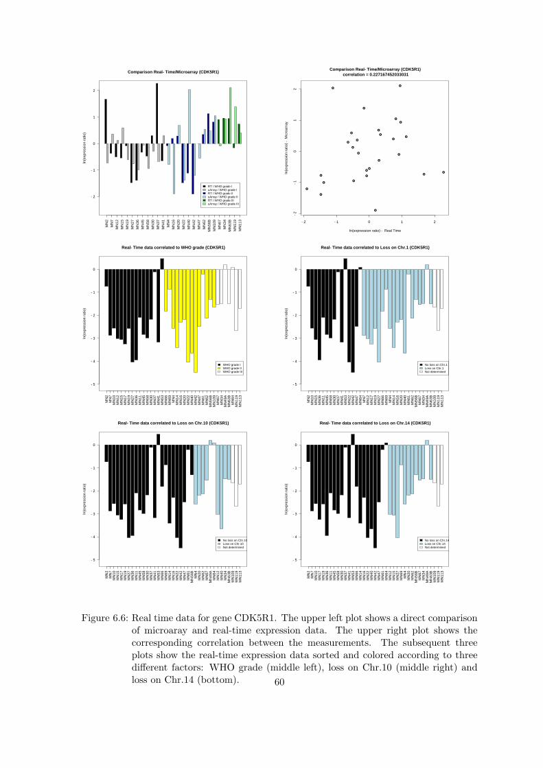
MN
2M
N7
MN
12M
N15
MN
19M
N27
MN
36M
N45
MN
58M
N30
MN
37M
N41
MN
4M
N16
MN
20M
N22
MN
40M
N42
MN
47M
N62
MN
56B
MN
109
MN
67M
N34
MN
63B
MN
119
MN
113
Comparison Real−Time/Microarray (CDK5R1)
ln(e
xpre
ssio
n ra
tio)
−2
−1
0
1
2
RT / WHO grade IuArray / WHO grade IRT / WHO grade IIuArray / WHO grade IIRT / WHO grade IIIuArray / WHO grade III
●
●
●
●
●
●
●
●
●
●
●
●
●
●
●
●
●
●
●
●●
●
●
●
●
●
●
−2 −1 0 1 2
−2
−1
01
2
Comparison Real−Time/Microarray (CDK5R1) correlation = 0.227167452033031
ln(expression ratio) − Real Time
ln(e
xpre
ssio
n ra
tio)
− M
icro
arra
y
MN
2M
N7
MN
10M
N12
MN
15M
N17
MN
19M
N27
MN
36M
N11
MN
45M
N58
MN
30M
N37
MN
41M
N53
MN
66M
N69
MN
4M
N14
MN
16M
N20
MN
22M
N40
MN
42M
N47
MN
61M
N62
MN
56B
MN
109
MN
67M
N34
MN
49A
MN
63B
MN
64M
N11
9M
N11
3
Real−Time data correlated to WHO grade (CDK5R1)
ln(e
xpre
ssio
n ra
tio)
−5
−4
−3
−2
−1
0
WHO grade IWHO grade IIWHO grade III
MN
2M
N10
MN
15M
N36
MN
11M
N45
MN
58M
N30
MN
37M
N41
MN
53M
N22
MN
42M
N47
MN
64M
N7
MN
12M
N17
MN
19M
N27
MN
66M
N69
MN
4M
N14
MN
16M
N20
MN
40M
N61
MN
62M
N56
BM
N67
MN
34M
N49
AM
N63
BM
N10
9M
N11
9M
N11
3
Real−Time data correlated to Loss on Chr.1 (CDK5R1)
ln(e
xpre
ssio
n ra
tio)
−5
−4
−3
−2
−1
0
No loss on Chr.1Loss on Chr.1Not determined
MN
2M
N7
MN
10M
N15
MN
17M
N19
MN
27M
N36
MN
11M
N45
MN
58M
N30
MN
37M
N41
MN
53M
N66
MN
69M
N14
MN
16M
N22
MN
42M
N47
MN
61M
N56
BM
N4
MN
20M
N62
MN
67M
N49
AM
N64
MN
12M
N40
MN
34M
N63
BM
N10
9M
N11
9M
N11
3
Real−Time data correlated to Loss on Chr.10 (CDK5R1)
ln(e
xpre
ssio
n ra
tio)
−5
−4
−3
−2
−1
0
No loss on Chr.10Loss on Chr.10Not determined
MN
2M
N7
MN
10M
N17
MN
19M
N36
MN
11M
N45
MN
58M
N30
MN
37M
N41
MN
53M
N66
MN
14M
N16
MN
22M
N40
MN
42M
N47
MN
61M
N64
MN
12M
N15
MN
27M
N69
MN
4M
N20
MN
62M
N56
BM
N67
MN
34M
N49
AM
N63
BM
N10
9M
N11
9M
N11
3
Real−Time data correlated to Loss on Chr.14 (CDK5R1)
ln(e
xpre
ssio
n ra
tio)
−5
−4
−3
−2
−1
0
No loss on Chr.14Loss on Chr.14Not determined
Figure 6.6: Real time data for gene CDK5R1. The upper left plot shows a direct comparisonof microaray and real-time expression data. The upper right plot shows thecorresponding correlation between the measurements. The subsequent threeplots show the real-time expression data sorted and colored according to threedifferent factors: WHO grade (middle left), loss on Chr.10 (middle right) andloss on Chr.14 (bottom). 60

MN
2M
N7
MN
10M
N12
MN
15M
N19
MN
27M
N36
MN
45M
N58
MN
30M
N37
MN
41M
N69
MN
4M
N14
MN
16M
N20
MN
22M
N40
MN
42M
N47
MN
62M
N56
BM
N10
9M
N67
MN
34M
N63
BM
N11
9M
N11
3
Comparison Real−Time/Microarray (VASP)
ln(e
xpre
ssio
n ra
tio)
−3
−2
−1
0
1
2
RT / WHO grade IuArray / WHO grade IRT / WHO grade IIuArray / WHO grade IIRT / WHO grade IIIuArray / WHO grade III
●
●
●
●
●
●
●
●
●
●
●●
●
●
●
●
●
●
●
●
●
●
●
●
●
●●
●
●
●
−1 0 1 2
−2
−1
01
2
Comparison Real−Time/Microarray (VASP) correlation = −0.333175649247361
ln(expression ratio) − Real Time
ln(e
xpre
ssio
n ra
tio)
− M
icro
arra
y
MN
2M
N7
MN
10M
N12
MN
15M
N17
MN
19M
N27
MN
36M
N11
MN
45M
N58
MN
30M
N37
MN
41M
N53
MN
66M
N69
MN
4M
N14
MN
16M
N20
MN
22M
N40
MN
42M
N47
MN
61M
N62
MN
56B
MN
109
MN
67M
N34
MN
49A
MN
63B
MN
64M
N11
9M
N11
3
Real−Time data correlated to WHO grade (VASP)
ln(e
xpre
ssio
n ra
tio)
−2.0
−1.5
−1.0
−0.5
0.0
0.5
1.0
WHO grade IWHO grade IIWHO grade III
MN
2M
N10
MN
15M
N36
MN
11M
N45
MN
58M
N30
MN
37M
N41
MN
53M
N22
MN
42M
N47
MN
64M
N7
MN
12M
N17
MN
19M
N27
MN
66M
N69
MN
4M
N14
MN
16M
N20
MN
40M
N61
MN
62M
N56
BM
N67
MN
34M
N49
AM
N63
BM
N10
9M
N11
9M
N11
3
Real−Time data correlated to Loss on Chr.1 (VASP)
ln(e
xpre
ssio
n ra
tio)
−2.0
−1.5
−1.0
−0.5
0.0
0.5
1.0
No loss on Chr.1Loss on Chr.1Not determined
MN
2M
N7
MN
10M
N15
MN
17M
N19
MN
27M
N36
MN
11M
N45
MN
58M
N30
MN
37M
N41
MN
53M
N66
MN
69M
N14
MN
16M
N22
MN
42M
N47
MN
61M
N56
BM
N4
MN
20M
N62
MN
67M
N49
AM
N64
MN
12M
N40
MN
34M
N63
BM
N10
9M
N11
9M
N11
3
Real−Time data correlated to Loss on Chr.10 (VASP)
ln(e
xpre
ssio
n ra
tio)
−2.0
−1.5
−1.0
−0.5
0.0
0.5
1.0
No loss on Chr.10Loss on Chr.10Not determined
MN
2M
N7
MN
10M
N17
MN
19M
N36
MN
11M
N45
MN
58M
N30
MN
37M
N41
MN
53M
N66
MN
14M
N16
MN
22M
N40
MN
42M
N47
MN
61M
N64
MN
12M
N15
MN
27M
N69
MN
4M
N20
MN
62M
N56
BM
N67
MN
34M
N49
AM
N63
BM
N10
9M
N11
9M
N11
3
Real−Time data correlated to Loss on Chr.14 (VASP)
ln(e
xpre
ssio
n ra
tio)
−2.0
−1.5
−1.0
−0.5
0.0
0.5
1.0
No loss on Chr.14Loss on Chr.14Not determined
Figure 6.7: Real time data for gene VASP. The upper left plot shows a direct comparisonof microaray and real-time expression data. The upper right plot shows thecorresponding correlation between the measurements. The subsequent threeplots show the real-time expression data sorted and colored according to threedifferent factors: WHO grade (middle left), loss on Chr.10 (middle right) andloss on Chr.14 (bottom). 61

MN
7M
N12
MN
15M
N19
MN
27M
N45
MN
58M
N30
MN
37M
N41
MN
69M
N4
MN
14M
N16
MN
20M
N22
MN
40M
N42
MN
47M
N62
MN
56B
MN
109
MN
67M
N34
MN
63B
MN
119
MN
113
Comparison Real−Time/Microarray (PTPRF)
ln(e
xpre
ssio
n ra
tio)
−4
−3
−2
−1
0
1
RT / WHO grade IuArray / WHO grade IRT / WHO grade IIuArray / WHO grade IIRT / WHO grade IIIuArray / WHO grade III
●
●
●
●
●
●
●
●●
●●
●
●
●
●
●
●
●
●
●
●
●
●
●
●
●
●
−2 −1 0 1 2
−3
−2
−1
01
Comparison Real−Time/Microarray (PTPRF) correlation = 0.338959483514593
ln(expression ratio) − Real Time
ln(e
xpre
ssio
n ra
tio)
− M
icro
arra
y
MN
2M
N7
MN
10M
N12
MN
15M
N17
MN
19M
N27
MN
36M
N11
MN
45M
N58
MN
30M
N37
MN
41M
N53
MN
66M
N69
MN
4M
N14
MN
16M
N20
MN
22M
N40
MN
42M
N47
MN
61M
N62
MN
56B
MN
109
MN
67M
N34
MN
49A
MN
63B
MN
64M
N11
9M
N11
3
Real−Time data correlated to WHO grade (PTPRF)
ln(e
xpre
ssio
n ra
tio)
−2
−1
0
1
2
3
4
5
WHO grade IWHO grade IIWHO grade III
MN
2M
N10
MN
15M
N36
MN
11M
N45
MN
58M
N30
MN
37M
N41
MN
53M
N22
MN
42M
N47
MN
64M
N7
MN
12M
N17
MN
19M
N27
MN
66M
N69
MN
4M
N14
MN
16M
N20
MN
40M
N61
MN
62M
N56
BM
N67
MN
34M
N49
AM
N63
BM
N10
9M
N11
9M
N11
3
Real−Time data correlated to Loss on Chr.1 (PTPRF)
ln(e
xpre
ssio
n ra
tio)
−2
−1
0
1
2
3
4
5
No loss on Chr.1Loss on Chr.1Not determined
MN
2M
N7
MN
10M
N15
MN
17M
N19
MN
27M
N36
MN
11M
N45
MN
58M
N30
MN
37M
N41
MN
53M
N66
MN
69M
N14
MN
16M
N22
MN
42M
N47
MN
61M
N56
BM
N4
MN
20M
N62
MN
67M
N49
AM
N64
MN
12M
N40
MN
34M
N63
BM
N10
9M
N11
9M
N11
3
Real−Time data correlated to Loss on Chr.10 (PTPRF)
ln(e
xpre
ssio
n ra
tio)
−2
−1
0
1
2
3
4
5
No loss on Chr.10Loss on Chr.10Not determined
MN
2M
N7
MN
10M
N17
MN
19M
N36
MN
11M
N45
MN
58M
N30
MN
37M
N41
MN
53M
N66
MN
14M
N16
MN
22M
N40
MN
42M
N47
MN
61M
N64
MN
12M
N15
MN
27M
N69
MN
4M
N20
MN
62M
N56
BM
N67
MN
34M
N49
AM
N63
BM
N10
9M
N11
9M
N11
3
Real−Time data correlated to Loss on Chr.14 (PTPRF)
ln(e
xpre
ssio
n ra
tio)
−2
−1
0
1
2
3
4
5
No loss on Chr.14Loss on Chr.14Not determined
Figure 6.8: Real time data for gene PTPRF. The upper left plot shows a direct comparisonof microaray and real-time expression data. The upper right plot shows thecorresponding correlation between the measurements. The subsequent threeplots show the real-time expression data sorted and colored according to threedifferent factors: WHO grade (middle left), loss on Chr.10 (middle right) andloss on Chr.14 (bottom). 62

MN
2
MN
7
MN
10
MN
12
MN
15
MN
19
MN
45
MN
58
MN
30
MN
41
MN
4
MN
14
MN
16
MN
20
MN
22
MN
42
MN
62
MN
56B
MN
109
MN
67
MN
34
MN
63B
MN
119
MN
113
Comparison Real−Time/Microarray (ELF3)
ln(e
xpre
ssio
n ra
tio)
−3
−2
−1
0
1
2
RT / WHO grade IuArray / WHO grade IRT / WHO grade IIuArray / WHO grade IIRT / WHO grade IIIuArray / WHO grade III
●
●
●
●
●
●
●
●
●
●
●
●
●
●
●
●
●
●
●
●
●
●
●
●
−1 0 1 2
−2
−1
01
Comparison Real−Time/Microarray (ELF3) correlation = −0.235226644657959
ln(expression ratio) − Real Time
ln(e
xpre
ssio
n ra
tio)
− M
icro
arra
y
MN
2M
N7
MN
10M
N12
MN
15M
N17
MN
19M
N27
MN
36M
N11
MN
45M
N58
MN
30M
N37
MN
41M
N53
MN
66M
N69
MN
4M
N14
MN
16M
N20
MN
22M
N40
MN
42M
N47
MN
61M
N62
MN
56B
MN
109
MN
67M
N34
MN
49A
MN
63B
MN
64M
N11
9M
N11
3
Real−Time data correlated to WHO grade (ELF3)
ln(e
xpre
ssio
n ra
tio)
−2
−1
0
1
2
3
WHO grade IWHO grade IIWHO grade III
MN
2M
N10
MN
15M
N36
MN
11M
N45
MN
58M
N30
MN
37M
N41
MN
53M
N22
MN
42M
N47
MN
64M
N7
MN
12M
N17
MN
19M
N27
MN
66M
N69
MN
4M
N14
MN
16M
N20
MN
40M
N61
MN
62M
N56
BM
N67
MN
34M
N49
AM
N63
BM
N10
9M
N11
9M
N11
3
Real−Time data correlated to Loss on Chr.1 (ELF3)
ln(e
xpre
ssio
n ra
tio)
−2
−1
0
1
2
3
No loss on Chr.1Loss on Chr.1Not determined
MN
2M
N7
MN
10M
N15
MN
17M
N19
MN
27M
N36
MN
11M
N45
MN
58M
N30
MN
37M
N41
MN
53M
N66
MN
69M
N14
MN
16M
N22
MN
42M
N47
MN
61M
N56
BM
N4
MN
20M
N62
MN
67M
N49
AM
N64
MN
12M
N40
MN
34M
N63
BM
N10
9M
N11
9M
N11
3
Real−Time data correlated to Loss on Chr.10 (ELF3)
ln(e
xpre
ssio
n ra
tio)
−2
−1
0
1
2
3
No loss on Chr.10Loss on Chr.10Not determined
MN
2M
N7
MN
10M
N17
MN
19M
N36
MN
11M
N45
MN
58M
N30
MN
37M
N41
MN
53M
N66
MN
14M
N16
MN
22M
N40
MN
42M
N47
MN
61M
N64
MN
12M
N15
MN
27M
N69
MN
4M
N20
MN
62M
N56
BM
N67
MN
34M
N49
AM
N63
BM
N10
9M
N11
9M
N11
3
Real−Time data correlated to Loss on Chr.14 (ELF3)
ln(e
xpre
ssio
n ra
tio)
−2
−1
0
1
2
3
No loss on Chr.14Loss on Chr.14Not determined
Figure 6.9: Real time data for gene ELF3. The upper left plot shows a direct comparisonof microaray and real-time expression data. The upper right plot shows thecorresponding correlation between the measurements. The subsequent threeplots show the real-time expression data sorted and colored according to threedifferent factors: WHO grade (middle left), loss on Chr.10 (middle right) andloss on Chr.14 (bottom). 63

Microarray data Real-time RT-PCR dataWHO grade I → II II → III I → II/III WHO grade I → II II → III I → II/III
Gene I II III p-val p-val p-val I II III p-val p-val p-valIGF2 -0.22 0.58 0.78 0.072 0.373 0.031 -0.49 1.13 1.09 0.627 0.729 0.277MDM4 -0.07 0.19 0.52 0.169 0.110 0.063 -0.25 0.57 0.49 0.145 0.692 0.022AKT3 -0.14 0.14 0.54 0.049 0.035 0.003 -0.11 0.31 0.33 -1.066 -0.823 0.564IGFBP3 -0.48 -0.12 0.88 0.077 0.017 0.004 -0.39 0.22 0.41 -2.062 -0.028 0.001CENPF -0.13 0.31 0.69 0.042 0.051 0.008 -0.16 0.57 0.67 2.124 3.551 0.000CDK5R1 0.06 0.14 0.60 0.320 0.041 0.065 -0.02 0.41 0.41 -2.363 -1.232 0.146VASP 0.13 -0.14 -0.13 0.007 0.561 0.002 -0.02 -0.02 0.31 -0.186 0.061 0.721PTPRF 0.25 -0.11 -0.17 0.015 0.361 0.002 0.06 -0.04 0.50 0.920 0.888 0.325ELF3 -0.01 -0.16 -0.26 0.038 0.202 0.011 -0.09 -0.15 0.19 -0.031 2.001 0.929
Table 6.1: Comparison of real time PCR and microarray expression data. The table showsthe means of expression according to tumorgrade. The p-values correspond tothe difference in means between grade I and II or grade II and III.
Microarray data Real-time RT-PCR data CorrelationGene Chr. NC Loss p-val NC Loss p-val Corr. Sign t-testIGF2 14 -0.49 1.13 0.00007 -0.16 1.50 0.00069 0.66 27/30 upr.MDM4 14 -0.25 0.57 0.00002 -0.23 0.58 0.00579 0.59 23/30 upr.AKT3 14 -0.11 0.31 0.00413 -1.14 -0.72 0.01914 0.24 19/29 upr.IGFBP3 10 -0.50 0.58 0.00052 -3.05 -0.60 0.00008 0.68 25/30 upr.CENPF 14 -0.16 0.57 0.00037 1.25 2.58 0.00864 0.53 22/30 upr.CDK5R1 10 -0.04 0.52 0.00036 -2.37 -1.83 0.09902 0.23 15/27 upr.VASP 14 -0.02 -0.02 0.49323 -0.17 -0.14 0.53793 -0.33 8/30 downr.PTPRF 1 0.33 -0.15 0.00006 1.30 0.78 0.11207 0.34 18/27 downr.ELF3 1 -0.03 -0.17 0.04999 -0.15 0.71 0.96992 -0.24 8/24 downr.
Table 6.2: Comparison of real time PCR and microarray expression data. The table iden-tifies the type of chromosomal aberration that each gene expression seems to beconnected to. In each case the p-value for the difference in means for the groupwith aberration compared to the group without the aberration (NC: no change)is given. The direct correlation between both datasets is given at the end of thetable as well as a comparison on the orientation of expression between real-timeand microarray data. The final column specifies the direction of the t-test (upr.:test for upregulated expression, downr.: test for downregulated expression)
The four genes IGF2, IGFBP3, MDM4 and CENPF show an acceptable correlation withthe microarray data. The correlation of expression with loss of genomic material presents averification of the earlier assumptions that were based on the microarray data. The p-valuesthat reflect the discrimination power of expression values with regard to the chromosomalaberrations are extremely low. IGFBP3 and CENPF also show a weak correlation withWHO grade. Taken together the RQ-PCR data corroborate the point that the expressionlevels show a tighter link to events on the genomic level than to the grading system.
64

7 Conclusions
The analysis of the meningioma expression data set presented here suggests two distinctpathways that might have a strong impact on meningioma pathogenesis. The link betweenexpression data and the specific chromosomal changes as presented here certainly needsfurther investigation and validation. But it is already interesting that for each pathway adistinct chromosomal loss with known significance for meningioma pathogenesis was iden-tified. Our analysis might provide a link to the functional implications of losses in theseregions.
The analysis also suggests that the relation between histological classification and thestate of gene expression of each sample are only loosely correlated. To further investigate thisrelationship the number of patient samples would probably need to be increased accordingly.
65
List of Figures
2.1 Highly expressed genes . . . . . . . . . . . . . . . . . . . . . . . . . . . . . . . 112.2 Random highly expressed genes . . . . . . . . . . . . . . . . . . . . . . . . . . 122.3 Gene with highest expression . . . . . . . . . . . . . . . . . . . . . . . . . . . 132.4 Genes with high expression . . . . . . . . . . . . . . . . . . . . . . . . . . . . 14
3.1 Shrunken centroid analysis of all grades - Cross validated error . . . . . . . . 163.2 Shrunken centroid analysis of grade I and III - Cross validated error . . . . . 173.3 Shrunken centroid analysis of grade I and III - Class probabilities . . . . . . . 183.4 Shrunken centroid analysis of grade I and III - Centroids . . . . . . . . . . . . 183.5 Shrunken centroid analysis on random data . . . . . . . . . . . . . . . . . . . 20
4.1 Expression values for IGFBP3 . . . . . . . . . . . . . . . . . . . . . . . . . . 364.2 Expression values for AKT3 . . . . . . . . . . . . . . . . . . . . . . . . . . . . 364.3 Expression values for IGF2 . . . . . . . . . . . . . . . . . . . . . . . . . . . . 374.4 Correlation of IGFBP3 and AKT3 . . . . . . . . . . . . . . . . . . . . . . . . 374.5 Correlation of IGFBP3 and AKT3 with loss on chr.10 . . . . . . . . . . . . . 424.6 Shrunken centroid analysis of chr.10 - Cross validated error . . . . . . . . . . 424.7 Shrunken centroid analysis of chr.10 - Class probabilities . . . . . . . . . . . . 434.8 Shrunken centroid analysis of chr.10 - Centroids . . . . . . . . . . . . . . . . . 44
5.1 Expression of WNT pathway related genes and tumor grade . . . . . . . . . . 495.2 Expression of WNT pathway related genes and loss of chromosome 14 . . . . 495.3 Expression of WNT pathway related genes and loss of chromosome 1 . . . . . 505.4 Expression of WNT pathway related genes and loss of chromosomes 1 and 14 505.5 Shrunken centroid analysis of chr.14 - Cross validated error . . . . . . . . . . 515.6 Shrunken centroid analysis of chr.14 - Class probabilities . . . . . . . . . . . . 525.7 Shrunken centroid analysis of chr.14 - Centroids . . . . . . . . . . . . . . . . . 53
6.1 Real time data for gene IGF2. . . . . . . . . . . . . . . . . . . . . . . . . . . . 556.2 Real time data for gene MDM4. . . . . . . . . . . . . . . . . . . . . . . . . . . 566.3 Real time data for gene AKT3. . . . . . . . . . . . . . . . . . . . . . . . . . . 576.4 Real time data for gene IGFBP3. . . . . . . . . . . . . . . . . . . . . . . . . . 586.5 Real time data for gene CENPF. . . . . . . . . . . . . . . . . . . . . . . . . . 596.6 Real time data for gene CDK5R1. . . . . . . . . . . . . . . . . . . . . . . . . 606.7 Real time data for gene VASP. . . . . . . . . . . . . . . . . . . . . . . . . . . 616.8 Real time data for gene PTPRF. . . . . . . . . . . . . . . . . . . . . . . . . . 626.9 Real time data for gene ELF3. . . . . . . . . . . . . . . . . . . . . . . . . . . 63
66

List of Tables
1.1 Parameters . . . . . . . . . . . . . . . . . . . . . . . . . . . . . . . . . . . . . 41.2 Experiments . . . . . . . . . . . . . . . . . . . . . . . . . . . . . . . . . . . . . 5
3.1 ROC I vs. II - Down-regulated . . . . . . . . . . . . . . . . . . . . . . . . . . 213.2 ROC I vs. II - Up-regulated . . . . . . . . . . . . . . . . . . . . . . . . . . . . 223.3 ROC I vs. III - Down-regulated . . . . . . . . . . . . . . . . . . . . . . . . . . 233.4 ROC I vs. III - Up-regulated . . . . . . . . . . . . . . . . . . . . . . . . . . . 243.5 ROC II vs. III - Down-regulated . . . . . . . . . . . . . . . . . . . . . . . . . 263.6 ROC II vs. III - Up-regulated . . . . . . . . . . . . . . . . . . . . . . . . . . . 273.7 ROC I and II vs. III - Down-regulated . . . . . . . . . . . . . . . . . . . . . . 283.8 ROC I and II vs. III - Up-regulated . . . . . . . . . . . . . . . . . . . . . . . 293.9 ROC I vs. II and III - Down-regulated . . . . . . . . . . . . . . . . . . . . . . 303.10 ROC I vs. II and III - Up-regulated . . . . . . . . . . . . . . . . . . . . . . . 32
3.11 EASE analysis of upregulated genes . . . . . . . . . . . . . . . . . . . . . . . 354.1 Genes positively correlated with IGFBP3 . . . . . . . . . . . . . . . . . . . . 394.2 Genes negatively correlated with IGFBP3 . . . . . . . . . . . . . . . . . . . . 39
5.1 Genes positively correlated with IGFBP3 . . . . . . . . . . . . . . . . . . . . 475.2 Genes negatively correlated with IGFBP3 . . . . . . . . . . . . . . . . . . . . 48
6.1 Real-Time / Microarray comparison I . . . . . . . . . . . . . . . . . . . . . . 646.2 Real-Time / Microarray comparison II . . . . . . . . . . . . . . . . . . . . . . 64
67

Bibliography
[Ben-Ze’ev et al., 2000] Ben-Ze’ev, A., Shtutman, M. & Zhurinsky, J. (2000) The integrationof cell adhesion with gene expression: the role of beta-catenin. Exp Cell Res, 261 (1),75–82.
[Bostrom et al., 1998] Bostrom, J., Cobbers, J. M., Wolter, M., Tabatabai, G., Weber,R. G., Lichter, P., Collins, V. P. & Reifenberger, G. (1998) Mutation of the PTEN(MMAC1) tumor suppressor gene in a subset of glioblastomas but not in meningiomaswith loss of chromosome arm 10q. Cancer Res, 58 (1), 29–33.
[Brabletz et al., 2002] Brabletz, T., Jung, A. & Kirchner, T. (2002) Beta-catenin and themorphogenesis of colorectal cancer. Virchows Arch, 441 (1), 1–11.
[Bright-Thomas & Hargest, 2003] Bright-Thomas, R. M. & Hargest, R. (2003) APC, beta-Catenin and hTCF-4; an unholy trinity in the genesis of colorectal cancer. Eur J SurgOncol, 29 (2), 107–117.
[Butt & Williams, 2001] Butt, A. J. & Williams, A. C. (2001) IGFBP-3 and apoptosis–alicense to kill. Apoptosis, 6 (3), 199–205.
[Cai et al., 2001] Cai, D. X., Banerjee, R., Scheithauer, B. W., Lohse, C. M., Kleinschmidt-Demasters, B. K. & Perry, A. (2001) Chromosome 1p and 14q FISH analysis in clinico-pathologic subsets of meningioma: diagnostic and prognostic implications. J NeuropatholExp Neurol, 60 (6), 628–636.
[Conover, 1992] Conover, C. A. (1992) Potentiation of insulin-like growth factor (IGF) ac-tion by IGF-binding protein-3: studies of underlying mechanism. Endocrinology, 130(6), 3191–3199.
[Conover et al., 2000] Conover, C. A., Bale, L. K., Durham, S. K. & Powell, D. R. (2000)Insulin-like growth factor (IGF) binding protein-3 potentiation of IGF action is mediatedthrough the phosphatidylinositol-3-kinase pathway and is associated with alteration inprotein kinase B/AKT sensitivity. Endocrinology, 141 (9), 3098–3103.
[Furstenberger & Senn, 2002] Furstenberger, G. & Senn, H.-J. (2002) Insulin-like growthfactors and cancer. Lancet Oncol, 3 (5), 298–302.
[Fujita et al., 2001] Fujita, M., Furukawa, Y., Tsunoda, T., Tanaka, T., Ogawa, M. & Naka-mura, Y. (2001) Up-regulation of the ectodermal-neural cortex 1 (ENC1) gene, a down-stream target of the beta-catenin/T-cell factor complex, in colorectal carcinomas. CancerRes, 61 (21), 7722–7726.
[Giles et al., 1998] Giles, R. H., Peters, D. J. & Breuning, M. H. (1998) Conjunction dys-function: CBP/p300 in human disease. Trends Genet, 14 (5), 178–183.
68

[Hirota et al., 1995] Hirota, S., Nakajima, Y., Yoshimine, T., Kohri, K., Nomura, S.,Taneda, M., Hayakawa, T. & Kitamura, Y. (1995) Expression of bone-related proteinmessenger RNA in human meningiomas: possible involvement of osteopontin in develop-ment of psammoma bodies. J Neuropathol Exp Neurol, 54 (5), 698–703.
[Howng et al., 2002] Howng, S.-L., Wu, C.-H., Cheng, T.-S., Sy, W.-D., Lin, P.-C. K., Wang,C. & Hong, Y.-R. (2002) Differential expression of Wnt genes, beta-catenin and E-cadherinin human brain tumors. Cancer Lett, 183 (1), 95–101.
[Huber et al., 2002] Huber, W., Von Heydebreck., A., Sultmann, H., Poustka, A. & Vin-gron, M. (2002) Variance stabilization applied to microarray data calibration and to thequantification of differential expression. Bioinformatics, 18 Suppl 1, S96–S104.
[Ihaka & Gentleman, 1996] Ihaka, R. & Gentleman, R. (1996) R: a language for data anal-ysis and graphics. J Comp Graph Stat, 5 (3), 299–314.
[Joachim et al., 2001] Joachim, T., Ram, Z., Rappaport, Z. H., Simon, M., Schramm, J.,Wiestler, O. D. & von Deimling., A. (2001) Comparative analysis of the NF2, TP53,PTEN, KRAS, NRAS and HRAS genes in sporadic and radiation-induced human menin-giomas. Int J Cancer, 94 (2), 218–221.
[Kachra et al., 1999] Kachra, Z., Beaulieu, E., Delbecchi, L., Mousseau, N., Berthelet, F.,Moumdjian, R., Del Maestro., R. & Beliveau, R. (1999) Expression of matrix metallo-proteinases and their inhibitors in human brain tumors. Clin Exp Metastasis, 17 (7),555–566.
[Kawashima et al., 2001] Kawashima, M., Suzuki, S. O., Yamashima, T., Fukui, M. & Iwaki,T. (2001) Prostaglandin D synthase (beta-trace) in meningeal hemangiopericytoma. ModPathol, 14 (3), 197–201.
[Khandwala et al., 2000] Khandwala, H. M., McCutcheon, I. E., Flyvbjerg, A. & Friend,K. E. (2000) The effects of insulin-like growth factors on tumorigenesis and neoplasticgrowth. Endocr Rev, 21 (3), 215–244.
[Kleihues et al., 1993] Kleihues, P., Burger, P. C. & Scheithauer, B. W. (1993) The newWHO classification of brain tumours. Brain Pathol, 3 (3), 255–268.
[Kwon et al., 2000] Kwon, Y. T., Gupta, A., Zhou, Y., Nikolic, M. & Tsai, L. H. (2000)Regulation of N-cadherin-mediated adhesion by the p35-Cdk5 kinase. Curr Biol, 10 (7),363–372.
[Leisch, 2002] Leisch, F. (2002) Sweave: dynamic generation of statistical reports usingliterate data analysis. In Compstat 2002 — Proceedings in Computational Statistics,(Hardle, W. & Ronz, B., eds), pp. 575–580 Physika Verlag, Heidelberg, Germany. ISBN3-7908-1517-9.
[Louis et al., 2000] Louis, D., Scheithauer, B., Budka, H., von Deimling, A. & Kepes, J.(2000) World Health Organization classification of tumours. Pathology and genetics oftumours of the nervous system. Lyon, France: IARC Press pp. 176–189.
[NG & Wong, 1993] NG, H. K. & Wong, A. T. (1993) Expression of epithelial and extra-cellular matrix protein markers in meningiomas. Histopathology, 22 (2), 113–125.
69

[Nordqvist & Mathiesen, 2002] Nordqvist, A.-C. S. & Mathiesen, T. (2002) Expression ofIGF-II, IGFBP-2, -5, and -6 in meningiomas with different brain invasiveness. J Neu-rooncol, 57 (1), 19–26.
[Pepe et al., 2003] Pepe, M. S., Longton, G., Anderson, G. L. & Schummer, M. (2003)Selecting differentially expressed genes from microarray experiments. Biometrics, 59(1), 133–142.
[Peters et al., 1998] Peters, N., Wellenreuther, R., Rollbrocker, B., Hayashi, Y., Meyer-Puttlitz, B., Duerr, E. M., Lenartz, D., Marsh, D. J., Schramm, J., Wiestler, O. D.,Parsons, R., Eng, C. & von Deimling., A. (1998) Analysis of the PTEN gene in humanmeningiomas. Neuropathol Appl Neurobiol, 24 (1), 3–8.
[Project Bioconductor, 2000] Project Bioconductor (2000). Project Bioconductor. http://www.bioconductor.org.
[Shimomura et al., 1996] Shimomura, A., Ogawa, Y., Kitani, T., Fujisawa, H. & Hagiwara,M. (1996) Calmodulin-dependent protein kinase II potentiates transcriptional activationthrough activating transcription factor 1 but not cAMP response element-binding protein.J Biol Chem, 271 (30), 17957–17960.
[Shinoura et al., 1994] Shinoura, N., Heffelfinger, S. C., Miller, M., Shamraj, O. I., Miura,N. H., Larson, J. J., DeTribolet, N., Warnick, R. E., Tew, J. J. & Menon, A. G. (1994)RNA expression of complement regulatory proteins in human brain tumors. Cancer Lett,86 (2), 143–149.
[Shtutman et al., 1999] Shtutman, M., Zhurinsky, J., Simcha, I., Albanese, C., D’Amico,M., Pestell, R. & Ben-Ze’ev, A. (1999) The cyclin D1 gene is a target of the beta-catenin/LEF-1 pathway. Proc Natl Acad Sci U S A, 96 (10), 5522–5527.
[Smith & Tsai, 2002] Smith, D. S. & Tsai, L. H. (2002) Cdk5 behind the wheel: a role intrafficking and transport. Trends Cell Biol, 12 (1), 28–36.
[Stambolic et al., 1998] Stambolic, V., Suzuki, A., de la. Pompa., J. L., Brothers, G. M.,Mirtsos, C., Sasaki, T., Ruland, J., Penninger, J. M., Siderovski, D. P. & Mak, T. W.(1998) Negative regulation of PKB/Akt-dependent cell survival by the tumor suppressorPTEN. Cell, 95 (1), 29–39.
[Watson et al., 2002] Watson, M. A., Gutmann, D. H., Peterson, K., Chicoine, M. R.,Kleinschmidt-DeMasters, B. K., Brown, H. G. & Perry, A. (2002) Molecular characteriza-tion of human meningiomas by gene expression profiling using high-density oligonucleotidemicroarrays. Am J Pathol, 161 (2), 665–672.
[Werner & Roberts, 2003] Werner, H. & Roberts, C. T. J. (2003) The IGFI receptor gene:a molecular target for disrupted transcription factors. Genes Chromosomes Cancer, 36(2), 113–120.
[Yamashima et al., 1997] Yamashima, T., Sakuda, K., Tohma, Y., Yamashita, J., Oda, H.,Irikura, D., Eguchi, N., Beuckmann, C. T., Kanaoka, Y., Urade, Y. & Hayaishi, O. (1997)Prostaglandin D synthase (beta-trace) in human arachnoid and meningioma cells: roles asa cell marker or in cerebrospinal fluid absorption, tumorigenesis, and calcification process.J Neurosci, 17 (7), 2376–2382.
70

[Zumkeller & Westphal, 2001] Zumkeller, W. & Westphal, M. (2001) The IGF/IGFBP sys-tem in CNS malignancy. Mol Pathol, 54 (4), 227–229.
71