mercatus graduate policy essay i would like to thank each of my mercatus graduate policy essay...

The opinions expressed in this Graduate Policy Essay are the author’s and do not represent official positions of the Mercatus Center or George Mason University.

No. 19 SUMMER 2015

MERCATUS GRADUATE POLICY ESSAY STATE FISCAL CONDITION AND INTERSTATE INCOME MIGRATION

by Scott Eastman

Abstract This analysis compares income migration to two measures of state fiscal condition with a state-level data set. This analysis focuses particularly on tax- and expense-burden differences (measurements of fiscal condition) between pairs of states. These data have almost 7,000 pairs of states that serve as observations. Each observation (pair) has an origin state that lost income and a destination state that received income from 2002 to 2010. This analysis finds that destination states with lower expense burdens (defined as total government spending per capita) and tax burdens (defined as total taxes levied per capita) relative to origin states consistently elicited more income migration than destination states with higher expense and tax burdens. This is so even when differences in factors like crime, weather, population, per capita income, demographics (race and age), unemployment, the proportion of a state’s industry devoted to natural resources, and tax code progressivity are controlled for. This analysis suggests state policymakers have control over at least one factor that affects migration patterns: the burden of government spending placed on taxpayers relative to other states.

Author Bio Scott Eastman is a program associate for the Project for the Study of American Capitalism and the State and Local Policy Project at the Mercatus Center. He received an MA in economics from George Mason University and is an alumnus of the Mercatus MA Fellowship program. Scott also holds a BA in political science from the University of Nebraska–Lincoln. As a Mercatus Center MA Fellow, Scott worked with scholars in Mercatus' State and Local Policy Project, as well as the Mercatus Center's Project for the Study of American Capitalism. Scott has interned with the Cato Institute’s Tax and Budget Policy department and worked as a policy analyst for Texas Public Policy Action during Texas’s 83rd Legislative Session, focusing primarily on taxation, budget, and health care policy.

Committee Members Jason Fichtner, senior research fellow, Mercatus Center at George Mason University Matthew Mitchell, senior research fellow and director, Project for the Study of American

Capitalism, Mercatus Center at George Mason University Eileen Norcross, senior research fellow and director, State and Local Policy Project, Mercatus

Center at George Mason University

Mercatus MA Fellows may select the Mercatus Graduate Policy Essay option in fulfillment of their requirement to conduct a significant research project. Mercatus Graduate Policy Essays offer a novel application of a well-defined economic theoretical framework to an underexplored topic in policy. Essays offer an in-depth literature review of the theoretical frame being employed, present original findings and/or analysis and conclude with policy recommendations. The views expressed here are not necessarily the views of the Mercatus Center or Mercatus Center Academic and Student Programs.

Acknowledgments I would like to thank each of my Mercatus Graduate Policy Essay committee members for all the time they contributed. I thank Matt Mitchell for taking the time to become familiar with the econometric component of this analysis and for all the feedback that made this analysis possible. I thank Eileen Norcross for helping me better understand the fiscal solvency variables that are featured in this analysis and for helping me sort out the policy implications of this analysis. And I thank my committee chair, Jason Fichtner, for keeping this on track and most importantly for investing so much time teaching me about tax policy throughout my time as a Mercatus MA Fellow.

Contents 1. Introduction ................................................................................................................................. 5 2. Literature Review: Fiscal Policy and Migration ......................................................................... 7 3. Data ........................................................................................................................................... 11 4. Model ........................................................................................................................................ 14 5. Results ....................................................................................................................................... 18 6. Discussion ................................................................................................................................. 27 7. Policy Prescription .................................................................................................................... 30 8. Conclusion ................................................................................................................................ 35 Appendix ....................................................................................................................................... 36

5

1. Introduction

The question of whether fiscal policy encourages migration has been a source of heated debate.

In the debate’s latest iteration, the American Legislative Exchange Council (ALEC) sparred with

the Center for Budget and Policy Priorities (CBPP) over whether taxation affects migration

decisions. The CBPP argued tax-rate differences have had little effect on migration and

encouraged policymakers to stop cutting taxes and focus on funding services that contribute to

the overall desirability of a location.1 ALEC, on the other hand, argued that taxation affects

migration by hampering economic growth, noting that businesses opt for states where they retain

more after-tax income for business operations and that individuals subsequently migrate to states

where businesses have located to take advantage of job opportunities.2

The following analysis contributes to this debate by comparing state fiscal conditions to

measures of income migration between states. As figure 1 shows, personal income migrated

from northeastern and midwestern states primarily to southeastern and western states from 2000

to 2010, with the large exception in the West being California. Figure 2 demonstrates the

magnitude of this trend in dollar terms by showing the top 10 state-to-state income flows over a

slightly shorter period, from 2002 to 2010. States like New York, New Jersey, Illinois, and

California lost billions to states like Florida, Texas, and Arizona.

1 Mazerov, Michael. “State Taxes Have a Negligible Impact on Americans’ Interstate Moves.” Center on Budget and Policy Priorities. May 21, 2014. Available at http://www.cbpp.org/cms/?fa=view&id=4141. The CBPP argues migration to southwestern and southern states in recent years was a function of job opportunities, cost of living differences, and weather. 2 Williams, Jonathan, Will Freeland, and Ben Wilterdink. “Taxes Do Matter to Migration.” American Legislative Exchange Council. May 12, 2014. Available at http://www.americanlegislator.org/policy-matters/. ALEC shows that the 10 states drawing the most migration over the past decade have seen an average job growth of 11.1 percent, compared to 1.8 percent for the 10 states losing the most people. The top 10 inflow states have received an average of 220,779 people and seen an average growth in Gross State Product (GSP) of 65.2 percent during this same time period, while the 10 states losing the most saw 411,176 taxpayers leave and GSP increase by only 45.7 percent.

6

These figures show a trend in income migration between states. The rest of this analysis

describes this trend with an econometric model that explains how differences in fiscal climates

affect income migration. In particular, this analysis shows that income migrated most often to

lower tax and lower spending states.

Figure 1

7

Top 10 Income Migration Flows Between States, 2002–2010 Origin State Destination State Net Income Gain

1. New York Florida $10.7 Billion 2. New Jersey Florida $6.79 Billion 3. New York New Jersey $6.78 Billion 4. California Nevada $4.79 Billion 5. California Arizona $4.96 Billion 6. California Texas $4.28 Billion 7. Ohio Florida $3.95 Billion 8. Illinois Florida $3.94 Billion 9. Pennsylvania Florida $3.81 Billion 10. California Oregon $3.6 Billion

Figure 2

2. Literature Review: Fiscal Policy and Migration

Migrants respond to both the taxation policies and the spending policies of state governments.

Each service government provides requires resources that increase the burden placed on

taxpayers. As the burden of government spending grows, the incentive for taxpayers to migrate

to less burdensome jurisdictions increases, particularly where there are large differences in

burdens between jurisdictions.3 This mobility promotes efficient service provision by

encouraging governments to compete for taxpayers, who are able to choose which jurisdiction

3 The efficient markets hypothesis, which normally is applied to financial markets, may be relevant to how migrants react to fiscal conditions. It would predict that taxpayers respond to abrupt changes in expense and tax burdens more than slow, steady growth in burdens. See Burton G. Malkiel. "The Efficient Market Hypothesis and Its Critics." Journal of Economic Perspectives 17.1 (2003): 59–82. Available at http://www.vixek.com/Efficient%20Market%20Hypothesis%20and%20its%20Critics%20-%20Malkiel.pdf. The theory of fiscal illusion might also explain why abrupt changes are more likely to spur migration. This theory extends the idea of rational ignorance to the individual’s perception of fiscal policy. Complicated tax and spending policies make it more difficult for taxpayers to discern the true cost of public services, contributing to growth in service provision as taxpayers fail to recognize the growing burden of fiscal policy as it accumulates. Abrupt changes, however, are more likely to alert people to the burdens of fiscal policy and thus spur migration. See James M. Buchanan and Richard E. Wagner. Democracy in Deficit. Academic Press, 1977. Available at http://www.econlib.org/library/Buchanan/buchCv8Cover.html.

8

they want to support.4 Governments that fail to maintain a tax base risk failure because of an

inability to extract resources to fund government spending.5

Research shows that people migrate out of higher tax states into lower tax states. Vedder

finds that in every state that increases its personal income-tax rate by 1 percentage point,

migration into that state drops by 100,000 people.6 The New Jersey Department of the Treasury

finds that a 2004 “millionaires” tax cost the state $2.5 billion in tax revenue, which left along

with 20,000 residents.7 Yakovlev finds higher personal income-tax rates to be associated with an

increased probability of residents moving to a state with a lower personal income-tax rate.8

Ruger and Sorens find their measures of fiscal freedom to be positively associated with net

migration, meaning that states with relatively lower tax burdens, levels of government

employment, and levels of government spending and debt draw more migrants than states with

less-free fiscal policy.9 Davies and Pulito focus particularly on how tax-rate differences between

states affect migration decisions and find that, for a period spanning 2006 to 2009, as high

marginal income-tax rates increased in surrounding states, a “home state” with a lower relative

rate experienced net in-migration.10

4 Tiebout, Charles M. "A Pure Theory of Local Expenditures." Journal of Political Economy 64.5 (1956): 416–424. 5 See Charles Levine’s discussion of “environmental entropy.” Charles H. Levine. "Organizational Decline and Cutback Management." Public Administration Review 38.4 (1978): 316–325. 6 Vedder, Richard. “Taxation and Migration.” Taxpayers Network. Available at http://www.taxpayersnetwork.org/_rainbow/documents/taxation%20and%20migration.pdf. 7 Lai, A., R. Cohen, and C. Steindel. “The Effect of Marginal Tax Rates on Interstate Migration in the U.S.” New Jersey Department of the Treasury, Oct. 2011. 8 Yakovlev, Pavel A. "State Economic Prosperity and Taxation." Mercatus Center at George Mason University. July 10, 2014. Available at http://mercatus.org/publication/state-economic-prosperity-and-taxation. 9 Ruger, William P., and Jason Sorens. “Freedom in the Fifty States: 2013 Edition.” Mercatus Center. 2013. Available at http://freedominthe50states.org/. The authors compare net interstate migration 2000–2010 to their measures of fiscal freedom, finding that migrants flow from states with less free fiscal policy to states with more free fiscal policy at statistically significant levels. 10 Davies, Antony, and John Pulito. “Tax Rates and Migration.” Mercatus Working Paper No. 11–31, 2011. The model employed by Davies and Pulito is of particular interest for this analysis. In this model, the authors examine how tax-rate differences between nearly 10,000 pairs of states affected migration patterns 2006–2009. Davies and Pulito use an ordinary least squares, panel data model that employs state-specific fixed effects to control for

9

Bakija and Slemrod investigate the effect of inheritance and estate taxes on the migration

of wealthy elderly taxpayers, finding that a 1 percentage point increase in inheritance and estate

taxes in a state was associated with a 1.4 to 2.7 percent reduction in the number of federal estate-

tax returns filed in that state, with the effect increasing as the size of an estate increased.11

Coomes and Hoyt also find a negative relationship between state income-tax rates and migration

in multistate metropolitan areas. These are areas that have cities along state borders, allowing

individuals to move relatively easily from one jurisdiction to another with little disruption, so

they can easily exploit differences in tax policy. The authors find that large differences in state

income-tax rates within multistate metropolitan areas affect migration.12

There are other factors that drive migration that must be considered in addition to fiscal

policy. Distance increases both the psychic and tangible costs of relocation, such as the cost of

obtaining information about potential relocation spots, which generates uncertainty and

discourages relocation. Individuals also consider factors like wages in the destination state, and

they react to factors like job loss in their current place of residence, as well as other factors like

the presence or absence of family ties in their origin and destination.13 Individuals also self-select

unobserved idiosyncratic differences between states, running their regression with dummy variables for each state. For a detailed discussion of this model, refer to the appendix. 11 Bakija, Jon, and Joel Slemrod. “Do the Rich Flee from High State Taxes? Evidence from Federal Estate Tax Returns.” National Bureau of Economic Research Working Paper No. 10645. 2004. Available at http://www.nber.org/papers/w10645.pdf. The authors find that returns from estates over $5 million declined by almost 4 percent in states that raised inheritance or estate taxes by 1 percent. 12 Coomes, Paul A., and William H. Hoyt. "Income Taxes and the Destination of Movers to Multistate MSAs." Journal of Urban Economics 63.3 (2008): 920–937. 13 Greenwood, Michael J. "Research on Internal Migration in the United States: A Survey." Journal of Economic Literature 13.2 (1975): 397–433. Importantly, such factors as wages and job loss can be the result of government institutions or rules. These may be tax policies, labor laws, or a number of other rules that can make a state attractive (or not attractive) in its job opportunities.

10

into areas offering the highest returns for their skills, particularly when they reside in areas that

offer poor returns for their skill endowment.14

Molloy, Smith, and Wozniak note some characteristics associated with people who are

more likely to move than others. They claim the “propensity to migrate” increases with

education but falls with age. Minorities and foreign-born persons, as well as households with one

child, are also less inclined to move, while renters (as opposed to homeowners) and unemployed

persons are more likely to move.15

Research by Greg Kaplan and Sam Schulhofer-Wohl also notes factors that have

contributed to a decline in migration. Technology (e.g., telecommuting) has decreased the need

to relocate for a job. Information technology and cheaper travel have reduced the cost of making

informed migration decisions, resulting in less migration. In other words, it is now easier for

people to travel to and learn about places, and people are finding they do not wish to move after

all. Decreasing migration might also be a function of increased productivity within occupations

and across states, which means people can realize increased productivity and higher incomes

without migrating.16

14 Borjas, George J., Stephen G. Bronars, and Stephen J. Trejo. "Self-Selection and Internal Migration in the United States." Journal of Urban Economics 32.2 (1992): 159–185. 15 Molloy, Raven, Christopher L. Smith, and Abigail K. Wozniak. “Internal Migration in the United States.” National Bureau of Economic Research Working Paper No. 17307, 2011. 16 Kaplan, Greg, and Sam Schulhofer-Wohl. “Understanding the Long-Run Decline in Interstate Migration.” National Bureau of Economic Research Working Paper No. 18507, 2012. The authors argue gross migration has declined because of a drop in the “geographic specificity of returns to occupations,” in turn because productivity is equalizing within occupations and across states. See also Raven Molloy, Christopher L. Smith, and Abigail K. Wozniak. “Internal Migration in the United States.” National Bureau of Economic Research Working Paper No. 17307, 2011.

11

3. Data

To examine income migration patterns, I use data from the IRS’s Statistics on Income database.17

The IRS tracks several migration measures using tax-return data for each calendar year, which

enables me to measure net income migration flows between states. The period I examine is from

2002 to 2010.18

The independent variables of interest—government expense and tax burdens—are part of

a set of “service-level solvency” measures that indicate the burden a state’s taxation and

spending policies place on taxpayers.19 These measurements were made possible by the

Governmental Accounting Standards Board’s (GASB) Statement No. 34, which requires state

and local governments to report information that can be used to assess the current and future

fiscal health of states on a “government-wide” basis.20 This information can be found annually in

Comprehensive Annual Financial Reports (CAFRs) for each state. This analysis focuses on tax

and expense burdens, defined as total taxes per person and total expenses per person. These

measurements are per capita figures, with higher per capita values theoretically signifying lower

service-level solvency and a reduced capacity to provide services relative to states with lower

17 Tax Foundation. “State to State Migration Data.” Available at http://interactive.taxfoundation.org/migration/. This tool aggregates migration data and makes it available in a format that is far easier to work with than the raw IRS data. For ease of collection, I used this tool. 18 In this analysis, I will examine only the effect expense and tax burdens have on income migration, although I provide an analysis of how these variables affect the migration of households and individuals in an appendix. 19 Wang, Xiaohu, Lynda Dennis, and Yuan Sen Jeff Tu. "Measuring Financial Condition: A Study of US States." Public Budgeting & Finance 27.2 (2007): 1–21. P. 4. Abstract available at http://papers.ssrn.com/sol3/papers.cfm?abstract_id=985696. Another variable, revenue burden, is also contained in this service-level solvency category, but I do not use it in this analysis because I want to focus strictly on taxes states levy and expenses states pay, whereas revenue includes such funds as grants from the federal government. 20 This government-wide requirement is an improvement from past methods of reporting financial condition that focused only on individual funds. While individual funds may be an accurate measure of financial condition for small organizations, individual funds (such as general revenue funds) represent small portions of a state government’s total spending. Wang’s measurements also gauge a government’s ability to generate liquid resources and cash to pay for current liabilities (cash solvency), its ability to generate revenue to sustain current services (budget solvency), and the effect a government’s current obligations will have on future resources (long-run solvency).

12

burdens.21 Using expense and tax burdens, it is possible to measure the size of each state

government and the burden it places on its population and compare measures of migration to the

differences in burdens across states. This allows us to see whether people and their income

migrate more frequently to states with lower burdens. Data on taxes and expenses were collected

from CAFRs from each state, and subsequently divided by population.22 These data span 48

states (they exclude the states of Alaska and Hawaii, as well as the District of Columbia) over

fiscal years 2002–2010.23

The fact that government expense and tax burdens are measured in fiscal years, as

opposed to the calendar years used with migration measures and control variables, calls for some

adjustment. I deal with this mismatch by lagging the tax and expense burden variables by at least

one fiscal year and up to five fiscal years to ensure the migration of income is being compared to

past burdens as much as possible. It would not make much sense to compare migration to

expense and tax burdens that occurred after migration.24

21 For a study that utilized these service-level solvency variables (as well as the other variables created by Wang, Dennis, and Tu) to rank the fiscal condition of states, see Arnett, Sarah. “State Fiscal Condition: Ranking the Fifty States.” Mercatus Working Paper No. 14–02, January 2014. Available at http://mercatus.org/sites/default/files/Arnett_StateFiscalCondition_v1.pdf. 22 These variables were calculated with taxation and spending amounts in thousands of dollars, and subsequently divided by the population of each state. This results in a smaller per capita figure but does not limit the use of these per capita figures to assess and compare the relative sizes of state governments and the burden these governments place on their respective populations. 23 Alaska was omitted because of concerns that it was subsidizing people to move there, which would have skewed the effect of these service-level solvency variables on migration relative to other states. Hawaii was omitted because of its distant location, and the District of Columbia was omitted because it did not produce a CAFR before 2006, meaning it would have far fewer data points than the rest of the states analyzed. Restricting studies of interstate migration to the 48 contiguous states is also standard. See Karen Smith Conway and Andrew J. Houtenville. "Elderly Migration and State Fiscal Policy: Evidence from the 1990 Census Migration Flows." National Tax Journal 54.1 (2001): 103–123. At p. 107. 24 The fiscal year ends on June 30 in all but four states. Michigan and Alabama have fiscal years that end on September 30, New York’s fiscal year ends on March 31, and Texas’s fiscal year ends on August 31. See National Conference of State Legislators, “Quick Reference Fiscal Table,” posted July 2000, reviewed July 13, 2012. Available at http://www.ncsl.org/research/fiscal-policy/basic-information-about-which-states-have-major-ta.aspx.

13

Ten control variables are used in this analysis, all of which are measured in calendar

years. Data from the Tax Foundation on the number of income-tax brackets in each state are used

to account for varying levels of progressivity in state tax codes.25 State population data were

collected from CAFRs to control for population-size differences between states (as well as to put

migration measures in per capita terms).26 Data on Gross Domestic Product by industry and by

state, as well as state personal income per capita, are available from the Bureau of Economic

Analysis, and are used to control for differences in the amount of industry dedicated to natural

resources and mining and for per capita income differences between states.27 Data from the

Bureau of Labor Statistics that track unemployment in the civilian noninstitutional population are

used to control for unemployment-rate differences between states.28 Census Bureau data are used

to control for demographic differences between states,29 and data from The Disaster Center

Crime Pages, which collects crime data from several government sources, including the

Department of Justice’s Bureau of Justice Statistics and the Federal Bureau of Investigation’s

Uniform Crime Reports, are used to control for differences in crime rates between states.30 Data

from the National Oceanic and Atmospheric Administration are used to control for weather

differences between states, specifically the difference in average January temperatures.31

25 Tax Foundation, “State Individual Income Tax Rates, 2000–2014.” April 1, 2013. Available at http://taxfoundation.org/article/state-individual-income-tax-rates. 26 Population data is available in other places, but I used population numbers for CAFRs to compute expense and tax burdens. 27 Bureau of Economic Analysis. “Regional Data.” Available at http://www.bea.gov/iTable/index_regional.cfm. 28 Bureau of Labor Statistics. “Civilian Non-Institutional Population and Associated Rate and Ratio Measures for Model-Based Areas.” Available at http://www.bls.gov/lau/rdscnp16.htm. 29 Historical race and age data from the Census Bureau can be found at http://www.census.gov/popest/data/historical/index.html. 30 Disaster Center Crime Pages. Available at http://www.disastercenter.com/crime/. The Index value that reports the total number of reported crimes per 100,000 people for each state is used to account for crime differences. 31 National Oceanic and Atmospheric Administration. “Climatological Rankings.” Available at http://www.ncdc.noaa.gov/temp-and-precip/climatological-rankings/index.php?periods%5B%5D=1&parameter=tavg&state=4&div=0&month=1&year=2002#ranks-form.

14

4. Model

Instead of focusing on tax-rate differentials, this analysis focuses on how differences in expense

and tax burdens between states affected income migration from 2002 to 2010. These data are

broken into pairwise observations providing between 3,056 and 6,775 observations, depending

on whether the model lags tax and expense burdens by one, two, three, four, or five fiscal years.

Income migration is regressed separately on expense and tax burdens. Regressions are run on

both the level of income migration and the natural log of income migration. Running regressions

on the natural log of income migration enables a percentage-change interpretation and adjusts for

the skewed nature of the data in level form. Taking the natural log rather than the levels of

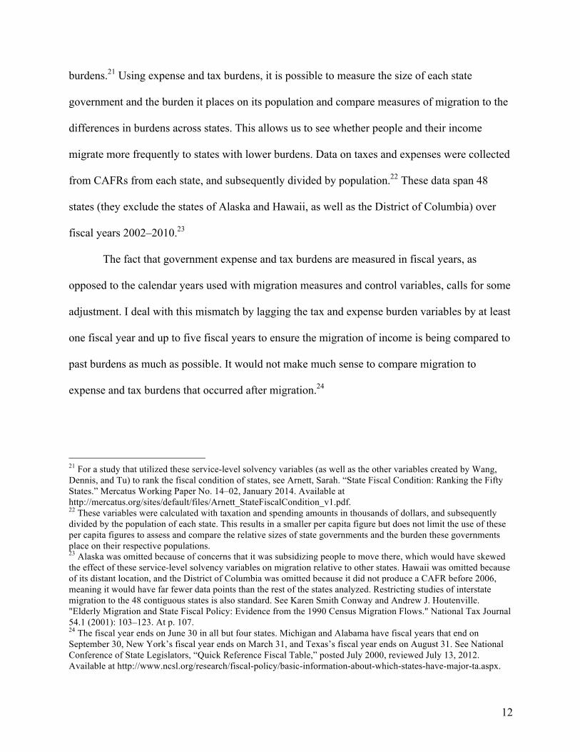
income migration also minimizes the importance of outliers. Below are two scatter plots that

show the relationship between income migration and expense burdens (lagged by five years):

one for when migration is measured in levels and another for when the natural log of income

migration is taken. The natural log of income migration is more normal, whereas the levels

scatter plot is skewed to the left.

15

Chart 1

050

100

150

200

250

-6 -4 -2 0 2 4ExpenseBurdenDifference, L

NetIncomePerCapita Fitted values

Level of Net Income Per Capita

16

Chart 2

Each observation includes both a destination state and an origin state, which are denoted

in the equations below by subscripts D and O. Year is denoted by subscript T. M stands for

migration of income into the destination state, and Ln(M) stands for the natural log of income

migration. Income migration in each year is divided by the population of the origin state that lost

income in the same year income migrated.32 E stands for expense burden, and T stands for tax

burden, while β1 is the coefficient for expense burden in equations 1 and 2 and for tax burden in

equations 3 and 4. For each equation, both the expense burden and tax burden variables are

lagged by one, two, three, four, and five years. For both burden variables, the subscript T is

32 Population estimates for states were also obtained from Comprehensive Annual Financial Reports. These states generally obtain data from the US Census Bureau, but some of the population estimates differed between CAFRs and the Census Bureau, although the differences were small.

-10

-50

5

-6 -4 -2 0 2 4ExpenseBurdenDifference, L

LogIncomeMigrationPerCapita Fitted values

Natural Log of Net Income Per Capita

17

subtracted by t, which signifies the burden is being lagged. This looks like β1ΔTD,O,T-t for tax

burden and β1ΔED,O,T-t for expense burden. X represents the 10 control variables discussed in

the data section (such as the difference in unemployment rate between states) and the Δ symbol

stands for the difference between these measures for each pairwise observation. Putting these

together, you get a vector of control variables denoted by ΔXD,O,Tβ, where β is the coefficient

on each control variable. Differences are generated by subtracting the origin-state value from the

destination-state value so that income migration is regressed on the differences between each

state pair’s expense and tax burdens, as well as the difference for each control variable. The term

ΘO-1 represents a vector of dummy variables for each origin state (minus one state to avoid

perfect collinearity), which I use to provide state-specific fixed effects, while ΩT-1 is a vector of

dummy variables for each year (again, minus one year) to provide for year fixed effects. The

expression ʯD,O,T is the error term. Only expense and tax burdens are lagged, and control

variables are contemporaneous with migration flows. Expense and tax burdens are highly

correlated, so they are run in separate regression models to ensure the effect of each burden on

migration is isolated as best as possible.33

The models used are provided below:

Equation 1: MD,O,T = α +β1ΔED,O,T-t + ΔXD,O,Tβ + ΘO-1 + ΩT-1 + ʯD,O,T

Equation 2: Ln(M) D,O,T = α +β1ΔED,O,T-t + ΔXD,O,Tβ + ΘO-1 + ΩT-1 + ʯD,O,T

33 See Wang, Xiaohu, Lynda Dennis, and Yuan Sen Jeff Tu. "Measuring Financial Condition: A Study of US States." Public Budgeting & Finance 27.2 (2007): 1–21. At pp. 10 and 15. The authors note that all of their variables measuring financial condition “should be correlated to ensure that they can be used to measure the same concept”—in this case, financial condition among states. They find their service-level solvency variables (including expense burdens and tax burdens) to be correlated.

18

Equation 3: MD,O,T = α +β1ΔTD,O,T-t + ΔXD,O,Tβ + ΘO-1 + ΩT-1 + ʯD,O,T

Equation 4: Ln(M)D,O,T = α +β1ΔTD,O,T-t + ΔXD,O,Tβ + ΘO-1 + ΩT-1 + ʯD,O,T

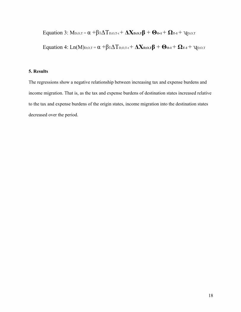
5. Results

The regressions show a negative relationship between increasing tax and expense burdens and

income migration. That is, as the tax and expense burdens of destination states increased relative

to the tax and expense burdens of the origin states, income migration into the destination states

decreased over the period.

19

Table 1

Regression Number 1 2 3 4 5VARIABLES Income Income Income Income Income

L.ExpenseBurdenDifference -‐0.699***(0.0908)

L2.ExpenseBurdenDifference -‐0.674***(0.0994)




PopulationDifference 4.61e-‐07*** 4.81e-‐07*** 4.79e-‐07*** 4.89e-‐07*** 4.55e-‐07***(3.17e-‐08) (3.51e-‐08) (3.84e-‐08) (4.11e-‐08) (3.18e-‐08)

NaturalShareDifference -‐0.0999*** -‐0.107*** -‐0.0864*** -‐0.0750*** -‐0.0751***(0.0130) (0.0135) (0.0140) (0.0148) (0.0141)

TaxBracketDifference -‐0.307*** -‐0.338*** -‐0.348*** -‐0.348*** -‐0.283***(0.0401) (0.0433) (0.0470) (0.0508) (0.0486)

PersonalIncomeDifference 0.000231*** 0.000242*** 0.000241*** 0.000200*** 0.000189***(3.15e-‐05) (3.36e-‐05) (3.57e-‐05) (3.50e-‐05) (3.02e-‐05)

UnemploymentDifference -‐0.905*** -‐0.999*** -‐0.932*** -‐0.881*** -‐0.546***(0.117) (0.123) (0.130) (0.134) (0.112)

HispanicDifference 0.0338*** 0.0290*** 0.0298*** 0.0354*** 0.0403***(0.00939) (0.00993) (0.0108) (0.0111) (0.0117)

AfricanAmericanDifference -‐0.0714*** -‐0.0662*** -‐0.0824*** -‐0.0542*** -‐0.0650***(0.0135) (0.0145) (0.0172) (0.0170) (0.0161)

Over65Difference 1.776*** 1.800*** 1.813*** 1.697*** 1.590***(0.133) (0.150) (0.166) (0.171) (0.171)

JanuaryTemperatureDifference 0.179*** 0.199*** 0.207*** 0.178*** 0.152***(0.0217) (0.0245) (0.0278) (0.0261) (0.0228)

CrimeDifference 0.000667*** 0.000454** 0.000488*** 0.000497*** 0.000489***(0.000155) (0.000177) (0.000183) (0.000189) (0.000185)

Constant 3.598*** 4.804*** 2.141** 3.164*** 1.897**(0.803) (0.934) (0.859) (0.585) (0.783)

State-‐Specific Fixed Effects YES YES YES YES YESYear Fixed Effects YES YES YES YES YESObservations 6,775 5,805 4,846 3,895 3,056R-‐squared 0.317 0.324 0.332 0.343 0.405Robust standard errors in parentheses*** p<0.01, ** p<0.05, * p<0.1

Expense Burdens and Income Migration

20

Table 2

Regression Number 6 7 8 9 10VARIABLES Log Income Log Income Log Income Log Income Log Income








TaxBracketDifference -‐0.0157** -‐0.0140** -‐0.0122 -‐0.0182** -‐0.00520(0.00650) (0.00699) (0.00779) (0.00921) (0.0101)

PersonalIncomeDifference 5.75e-‐05*** 5.98e-‐05*** 6.48e-‐05*** 5.64e-‐05*** 6.57e-‐05***(4.96e-‐06) (5.31e-‐06) (5.61e-‐06) (6.11e-‐06) (6.47e-‐06)

UnemploymentDifference -‐0.0206 -‐0.0213 0.000975 0.0136 0.0407**(0.0155) (0.0158) (0.0164) (0.0183) (0.0196)

HispanicDifference 0.00974*** 0.00672*** 0.00493** 0.00441* 0.00312(0.00203) (0.00221) (0.00237) (0.00260) (0.00294)

AfricanAmericanDifference 0.000845 -‐0.00163 -‐0.00738** -‐0.00792** -‐0.0176***(0.00266) (0.00289) (0.00328) (0.00368) (0.00414)

Over65Difference 0.0721*** 0.0558*** 0.0392*** 0.0324** 0.0189(0.0104) (0.0112) (0.0129) (0.0140) (0.0158)


CrimeDifference 0.000359*** 0.000372*** 0.000401*** 0.000406*** 0.000428***(2.68e-‐05) (3.09e-‐05) (3.41e-‐05) (3.86e-‐05) (4.50e-‐05)

Constant -‐0.638*** -‐0.311 -‐0.862*** -‐0.819*** -‐0.979***(0.175) (0.205) (0.207) (0.198) (0.208)


Expense Burdens and Log Income

21

Table 3

Regression Number 11 12 13 14 15VARIABLES Income Income Income Income Income

L.TaxBurdenDifference -‐0.513***(0.175)

L2.TaxBurdenDifference -‐0.286(0.187)

L3.TaxBurdenDifference -‐0.334*(0.202)

L4.TaxBurdenDifference -‐0.430**(0.218)

L5.TaxBurdenDifference -‐0.483**(0.232)



TaxBracketDifference -‐0.353*** -‐0.395*** -‐0.408*** -‐0.417*** -‐0.356***(0.0403) (0.0447) (0.0477) (0.0536) (0.0513)

PersonalIncomeDifference 0.000213*** 0.000214*** 0.000216*** 0.000177*** 0.000172***(3.10e-‐05) (3.37e-‐05) (3.60e-‐05) (3.59e-‐05) (3.23e-‐05)

UnemploymentDifference -‐1.053*** -‐1.118*** -‐1.028*** -‐0.963*** -‐0.623***(0.115) (0.125) (0.133) (0.139) (0.118)

HispanicDifference 0.0122 0.00869 0.00673 0.0119 0.0173(0.00868) (0.00915) (0.0101) (0.0103) (0.0108)

AfricanAmericanDifference -‐0.0820*** -‐0.0771*** -‐0.0933*** -‐0.0612*** -‐0.0752***(0.0137) (0.0148) (0.0176) (0.0172) (0.0162)

Over65Difference 1.669*** 1.686*** 1.672*** 1.550*** 1.443***(0.126) (0.141) (0.154) (0.160) (0.160)


CrimeDifference 0.000768*** 0.000533*** 0.000575*** 0.000582*** 0.000562***(0.000152) (0.000174) (0.000180) (0.000188) (0.000185)

Constant 2.760*** 3.938*** 4.262*** 1.870*** 0.679(0.771) (0.897) (0.883) (0.564) (0.779)


Tax Burdens and Income Migration

22

Table 4

Regression Number 16 17 18 19 20VARIABLES Log Income Log Income Log Income Log Income Log Income


L2.TaxBurdenDifference -‐0.236***(0.0430)






TaxBracketDifference -‐0.0225*** -‐0.0215*** -‐0.0166** -‐0.0237** -‐0.0100(0.00656) (0.00704) (0.00780) (0.00927) (0.0102)


UnemploymentDifference -‐0.0545*** -‐0.0411*** -‐0.00878 0.00852 0.0365*(0.0152) (0.0157) (0.0163) (0.0181) (0.0196)

HispanicDifference 0.00386* 0.00123 -‐0.000438 -‐0.000903 -‐0.00247(0.00198) (0.00215) (0.00233) (0.00253) (0.00289)

AfricanAmericanDifference -‐0.00174 -‐0.00417 -‐0.00964*** -‐0.00994*** -‐0.0207***(0.00267) (0.00289) (0.00330) (0.00369) (0.00417)

Over65Difference 0.0499*** 0.0345*** 0.0188 0.0114 -‐0.00248(0.0104) (0.0111) (0.0128) (0.0138) (0.0155)



Constant -‐0.827*** -‐0.483** -‐0.614*** -‐1.009*** -‐1.194***(0.173) (0.203) (0.211) (0.201) (0.204)


Tax Burdens and Log Income

23

Summary Statistics

Table 5

For instance, the average destination state received $3.79 per capita in income migration

over the period. The model based on equation 1 (shown in table 1) predicts that if the average

destination state’s expense burden increased by one standard deviation relative to the origin state

one fiscal year prior to migration (regression 1), the average destination state would see income

migration decrease by $1.09 per capita, decreasing income migration to $2.70 per capita, ceteris

paribus.34 This effect generally increases as expense burden is lagged by additional years.

Regression 5 predicts that a one standard deviation increase in the average destination state’s

expense burden relative to the origin state, five fiscal years prior to migration, would reduce

income migration by $1.50, to approximately $2.29 per capita.35

The effect of tax burdens on the level of income migration (equation 3, shown in table 3)

moves in the same direction, although the magnitude of the effect is smaller and the estimations

34 1.56 x –$.70 = –$1.09. Then, $3.79 – $1.09 = $2.70. Numbers are rounded at the second decimal place. Values for all these variables can be found in the summary statistics. 35 1.56 x –$.96 = –$1.50. Then, $3.79 – $1.09 = $2.29.

Variable Observation Mean Standard Deviation Minimum MaximumNetIncomePerCapita 10152 3.792061 9.385367 0 234.5411LogIncomeMigrationPerCapita 10150 0.039814 1.694336 -‐8.6548 5.457631ExpenseBurdenDifference 10152 -‐0.3445 1.558279 -‐5.68772 5.030799TaxBurdenDifference 10152 -‐0.16849 0.8022909 -‐3.93423 3.889067PopulationDifference 10152 -‐1164341 9362585 -‐3.68E+07 3.67E+07NaturalShareDifference 10152 1.324206 7.428854 -‐39.7997 40.68332TaxBracketDifference 9024 -‐0.13564 3.981254 -‐10 10PersonalIncomeDifference 10152 -‐2054.33 6938.863 -‐26389 22083UnemploymentDifference 10152 -‐0.07878 1.610051 -‐9.6 7.5HispanicDifference 10152 1.153321 13.6538 -‐43.7679 44.32125AfricanAmericanDifference 10152 0.084024 13.62638 -‐36.3251 36.43007Over65Difference 9024 -‐0.20589 2.142749 -‐8.21977 8.488168JanuaryTemperatureDifference 10231 3.840074 15.66906 -‐66 63.1CrimeDifference 9021 372.9887 1212.812 -‐4064 4353.9

24

are less significant (the estimations of expense burdens were statistically significant at the 99

percent level for regressions 1–5, whereas only regression 11 is statistically significant at the 99

percent level for tax burdens). Also, lagging tax burdens yields a smaller coefficient than the

one–fiscal year lagged model. Regression 11 predicts that a one standard deviation increase in

the tax burden of the average destination state relative to the origin state would reduce income

migration by $0.41, to $3.38 per capita.36 Regression 15 predicts that a one standard deviation

increase in the tax burden of the destination state relative to the origin state five years prior to

migration would reduce income migration by $0.38, to $3.41 per capita.37

There are two variables with coefficients that consistently meet or exceed the coefficients

of expense and tax burdens: differences in unemployment rate between destination states and

origin states, and differences in the share of the population over age 65. Even so, expense

burdens have a larger coefficient than unemployment rate in both the four– and five– fiscal year

lagged models (regression 4 and regression 5). Also, in regressions 12 and 13, the difference in

income-tax brackets between states has a larger coefficient and is more statistically significant

than the tax burden variable, and the coefficients for unemployment-rate differences and the

difference in population over 65 are larger than the coefficient on tax burdens in regressions 11

through 15.

Taken together, both expense and tax-burden differences generally have a statistically

significant effect on income migration levels, although expense-burden differences at the state

level have a larger effect on income migration levels than do tax burdens. The magnitude of this

effect is large compared to differences in crime, weather, personal income per capita, natural

resource exploitation, and race composition between states but is overshadowed by differences in

36 .80 x –$.51 = –$.41. Then, $3.79 – $.41 = $3.38. 37 .80 x –$.48 = $.38. Then, $3.79 – $.38 = $3.41.

25

the unemployment rate and prevalence of older people between states. Also, lagging expense and

tax burdens generally increases the effect expense and tax burdens have on the level of income

migration, and these variables generally remain statistically significant.

The log of income migration (equation 2 and equation 4, tables 2 and 4) shows that

increases in burdens have a larger percentage-change effect than increases in any other variable.

Regressions predict that increases in the average destination states’ expense and tax burden

relative to the origin state yield a larger percentage change in income per capita than does any

other variable.

Again, take the average state. The average destination state saw a 3.9 percent increase in

income migration over this period. Using the coefficient for percentage change in regression 6,

the regression based on equation 2 predicts that a one standard deviation increase in the

destination states’ expense burden relative to the origin states’ expense burden one fiscal year

prior to migration would result in a 30 percent decrease in income migration into the destination

state.38 This result increases when expense burdens are lagged by five fiscal years (regression

10), in which case a one standard deviation increase in the destination state’s expense burden

would decrease income migration by 33 percent.

The same pattern holds for tax burdens.39 A one standard deviation increase in the

destination state’s tax burden relative to the origin state’s one year prior to migration (regression

16, based on equation 4) would decrease income migration by 19 percent,40 whereas a one

standard deviation increase five years prior to migration would decrease income migration by 28

percent (regression 20).41 Comparing these percentage changes to the average for all destination

38 1.56 x –.19 = –.30 or –30%. 39 1.56 x –.21 = –.33 or –33%. 40 .80 x –.24 = –.19 or –19%. 41 .80 x –.35 = –.28 or –28%.

26

states is important. Again, the average destination state in this period actually saw a 3.9 percent

increase in income migration per capita. These regressions show that increasing expense and tax

burdens by one standard deviation quickly reduces the income migrating into these destination

states.

It is important to note that percentage changes say nothing about the importance of one

variable over another in terms of level effects, and as the discussion of income migration levels

above shows, there are other variables in the model that account for higher levels of income

migration. This relationship is analogous to economic growth rates in rich and poor nations. Poor

nations are able to grow at faster rates than rich nations because it is easier to grow a smaller

economy in percentage-change terms than it is to grow a larger economy. This does not change

the fact that larger economies still have a higher level of absolute wealth than faster-growing but

poorer nations. In terms of income migration, the regressions dealing with levels of income show

that differences between destination states and origin states in the unemployment rate and in the

amount of population over the age of 65 account for a higher level of income migration, even

while increases in tax and expense burdens yield the largest percentage-change values.

Still, the fact that increases in expense and tax burdens are associated with decreased

income migration into destination states is important. This is because policymakers have some

control over tax and expense burdens, meaning they can take some steps toward increasing

income migration by lowering expense and tax burdens. Also, because government spending

crowds out the resources available to businesses to invest and operate, increasing these burdens

might increase the unemployment rate, a variable that is also associated with negative income

migration. This suggests policymakers can make their states more attractive destinations for

migrants by reducing the size of their governments relative to other states.

27

6. Discussion

One drawback to this analysis is endogeneity. In “Tax Rates and Migration,” Davies and Pulito

explain that there was a significant amount of “bi-directionality” in the relationship between tax

rates and migration. It may be that high tax rates drive people to migrate to a less burdensome

state, but Davies and Pulito note that this movement reduces a state’s tax base, necessitating

higher tax rates on the people who remain to provide services. This creates a feedback loop

where higher tax rates drive migration, which, in turn, encourages the state to raise taxes to

recoup revenue, meaning high tax rates spur migration and this migration in turn leads to higher

tax rates.42

Bi-directionality is a concern in this analysis also. High expense and tax burdens might

encourage people to move. This outflow of people would make expense and tax burdens

increase. Population outflow decreases the denominator used to divide total taxes and total

expenditures, meaning the migration of people actually puts upward pressure on the independent

variable that theoretically should affect migration. Lagging variables partly addresses these

endogeneity concerns between income migration and tax and expense burdens. Lagging

variables also makes it easier to say it is tax and expense burdens influencing migration, rather

than the opposite, because migration cannot affect burdens from five years prior to that

migration.

Regardless of this endogeneity problem, the effect of tax-base erosion on expense and tax

burdens is important for the taxpayers who choose not to or cannot migrate in response to

increasing burdens. Tax-base erosion increases the expense and tax burdens on taxpayers who

cannot move, meaning fewer people are left to support government services. This requires more

42 Davies, Antony, and John Pulito. “Tax Rates and Migration.” Mercatus Working Paper No. 11–31, 2011. At p. 22.

28

from each taxpayer or a reduction in services if a state is to balance revenues with expenditures.

Any failure to do this results in debt, a poor state of fiscal health for origin states, and higher

burdens for remaining residents (both in terms of debt, if a state keeps spending, and forfeited

services, if states make spending cuts).

This scenario has played out at both the state and local levels when governments have

failed to balance revenues with expenditures. Detroit, Michigan, had a population of 2 million at

its 1950 peak, but this population fell over the next six decades to around 750,000.43 In the

summer of 2013, the municipality became the largest US city to declare bankruptcy, doing so as

its dwindling and impoverished population was unable to pay the city’s obligations.44 The city’s

pension problem was particularly bad, as the benefits owed to the city’s 21,000 retirees reached

$3.5 billion and became the “second biggest drain on the city’s bank account,” all while the

number of workers available to pay into the city’s pension systems fell.45

As the Detroit example shows, dwindling tax bases can be destructive for governments

that have promised payouts to beneficiaries but lost the population necessary to pay for those

benefits. This stress can be seen in state pension systems. State Budget Solutions estimates state

public pension plans are underfunded by $4.7 trillion, or about $15,000 for every person in the

United States, and notes that taxpayers throughout the country will feel this burden, as state

governments will have to allocate resources toward these obligations and away from services.

States currently are struggling to fund their pension systems, with Illinois, Connecticut, and

43 “How to Break an American City.” Reason. November 2013. Available at http://reason.com/archives/2013/10/21/how-to-break-an-american-city. 44 Plumer, Brad. “Detroit Just Filed for Bankruptcy. Here’s How It Got There.” Washington Post. July 18, 2013. Available at http://www.washingtonpost.com/blogs/wonkblog/wp/2013/07/18/detroit-just-filed-for-bankruptcy-heres-how-it-got-there/. 45 “Editorial: How Detroit Came to Betray Its Retirees.” Detroit Free Press. July 14, 2013. Available at http://www.freep.com/article/20130714/OPINION01/307140047/detroit-pensions-financial-crisis-retirees.

29

Kentucky being the three states with the lowest funding ratios—at 22 percent, 23 percent, and 24

percent, respectively. Alaska places the largest unfunded liability on its residents, at about

$40,000 per capita, followed by Illinois at almost $26,000 and Ohio at just over $25,000.46

Poor pension performance and poor fiscal performance in general at the state level have

been reflected in credit downgrades. Illinois suffered 13 credit downgrades from 2009 to 2013,

owing largely to the state’s massively underfunded pension system.47 And Illinois policymakers

have opted to raise fees and taxes to fill in pension gaps instead of making structural reforms that

would make the system more sustainable, such as raising the age at which pension beneficiaries

can receive benefits.48 In September 2014, Fitch Ratings downgraded New Jersey’s credit rating

after Governor Chris Christie opted to plug a budget gap by redistributing $2.4 billion from the

state’s pension system, showing that fiscal problems elsewhere in the budget can also negatively

impact the ability of governments to meet pension obligations.49 Kansas experienced a credit

downgrade in 2014 when Standard & Poor’s lowered the state’s bond rating from AA+ to AA,

citing failure to match income-tax cuts with cuts in spending.50

46 Luppino-Esposito, Joe. “Promises Made, Promises Broken 2014: Unfunded Liabilities Hit $4.7 Trillion.” State Budget Solutions. Nov. 12, 2014. Available at http://www.statebudgetsolutions.org/publications/detail/promises-made-promises-broken-2014-unfunded-liabilities-hit-47-trillion. 47 Klingner, John. “Illinois Has Lowest Credit Rating of All 50 States.” Illinois Policy Institute. Nov. 19, 2013. Available at https://www.illinoispolicy.org/illinois-has-lowest-credit-rating-of-all-50-states/. 48 Dabrowski, Ted. “Parks and Wreck.” Illinois Policy Institute. Nov. 7, 2013. Available at https://www.illinoispolicy.org/parks-and-wreck/?utm_source=Illinois+Policy+Institute&utm_campaign=14476f51fb-0615_HPP_pensions&utm_medium=email&utm_term=0_0f5a22f52c-14476f51fb-10656193. 49 Rizzo, Salvador. “Fitch Downgrades N.J. Debt, Saying Christie Is Repudiating His Pension Reform.” NJ.com. Sep. 5, 2014. 50 Lowry, Bryan. “S&P Downgrades Kansas Bond Rating; Brownback Pushes Back.” Aug. 6, 2014. Available at http://www.kansas.com/news/article1158214.html.

30

7. Policy Prescription

Even though this analysis cannot claim to show that expense and tax burdens cause migration, it

provides more evidence supporting the idea that increasing the burden of government spending

makes a state less attractive to taxpayers. This means states should think carefully about what

services to spend on, because every tax dollar spent increases the incentive for taxpayers to move

to a less burdensome state.

Are there any areas of government spending that migrants prefer more than others? My

data can be used to make a few suggestions on how states should organize spending to attract

migrants. The National Association of State Budget Officers (NASBO) documents the

composition of state budgets, measuring the proportion of budgets in seven categories:

elementary and secondary education, higher education, public assistance, Medicaid, corrections,

transportation, and a catchall that captures all other spending.

The following scatter plots qualitatively compare how the proportion of state budgets

allocated to public assistance relates to expense burdens, tax burdens, and income migration. The

graphs demonstrate a positive relationship between the amount of its budget a state allocates to

public assistance and the state’s total expense and tax burdens. As public assistance funding

rises, so do expense and tax burdens. Conversely, the graph comparing public assistance funding

to income migration shows a negative relationship, where income tends to flow out of a state as

that state’s spending on public assistance rises.51

51 The value for the proportion of state budgets going toward public assistance is lagged by one fiscal year when compared to income migration to ensure migration is being compared to budget composition data from the past. The scatter plots comparing public assistance to expense and tax burdens are not lagged because both are measured in fiscal years.

31

Chart 3

Chart 4

0.001.002.003.004.005.006.007.008.009.00

10.00

0.00 1.00 2.00 3.00 4.00 5.00 6.00 7.00

Expense Burden and Public Assistance Spending

0.00

1.00

2.00

3.00

4.00

5.00

6.00

0.00 1.00 2.00 3.00 4.00 5.00 6.00 7.00

Tax Burden and Public Assistance Spending

32

Chart 5

Thus, the proportion of state budgets going toward public assistance is associated with

increased tax and expense burdens, as well as a decrease in the amount of income flowing into

states (negative values on the Y axis represent states that had net income migration outflow,

whereas positive values represent states that had net income migration inflows). While it may be

undesirable to suggest a state stop spending on public assistance entirely, states might focus on

ways of providing public assistance in more efficient ways in order to reduce the amount of

taxation and spending required to sustain their public-assistance policies. How a state might

actually do that is far beyond the scope of this analysis.

It is also important to note a few things about this interpretation. First, public assistance

spending generally constituted a smaller part of state budgets than the other five budgetary

categories (excluding the catchall), with the highest proportion of budget expenditures dedicated

to public assistance standing at about 6.5 percent. This means there is less absolute room to cut

public assistance spending than other budgetary areas.

-800

-600

-400

-200

0

200

400

600

800

0.00 1.00 2.00 3.00 4.00 5.00 6.00 7.00

Income Migration and Public Assistance Spending

33

Second, this correlation between public assistance spending and income migration might

be capturing other factors that could spur migration. For instance, increased public assistance

expenditures might mean a state’s population is relatively impoverished compared to other

states. This might encourage wealthier taxpayers to leave because they dislike living in a state

with higher amounts of poverty.

Third, a majority of the funds states spent on public assistance comes from the federal

government, going toward programs like Temporary Assistance for Needy Families (TANF).52

This suggests migration has more to do with factors like poverty and less with the taxes states

levy to finance public assistance spending.

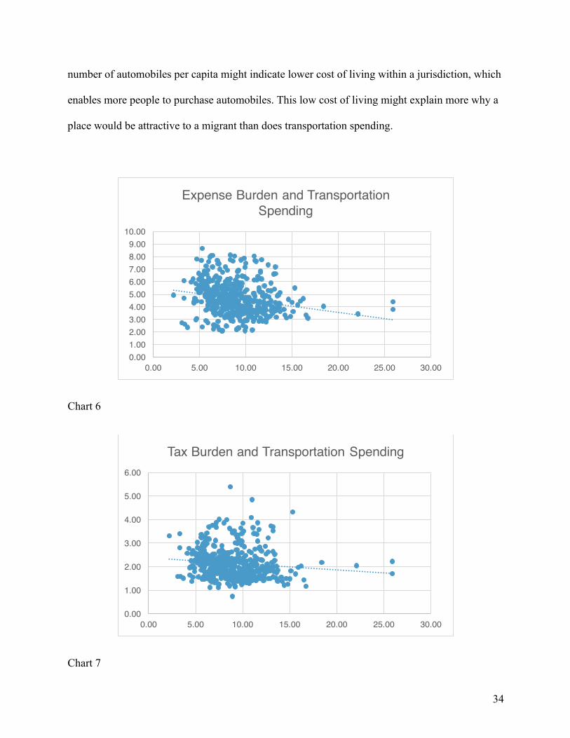
We can also examine other budget areas that draw less funding from the federal

government, such as transportation spending. Transportation is funded more by state funds and

less by federal funds, although federal funds still made up an average of 30 percent of state

spending over the period measured. The scatter plots below show that states that dedicate more

funds to transportation spending generally have lower expense and tax burdens and draw more

income migration. If transportation draws people and their money in, a focus on funding

transportation might actually put states on firmer fiscal ground by increasing their tax base. Still,

correlation does not mean causation, and there may be other reasons why migrants have chosen

states that devote a higher proportion of their budgets to transportation. It might be that states

that dedicate more to transportation have a higher number of automobiles per capita. A higher

52 See “State Expenditure Report: Examining Fiscal 2012–2014 State Spending.” National Association of State Budget Officers, 2014. Available at http://www.nasbo.org/sites/default/files/State%20Expenditure%20Report%20%28Fiscal%202012-2014%29S.pdf. Federal funds accounted for an average of 28.69 percent of total spending across states from fiscal years 2002 to 2010. The amount of federal funds per budgetary category varied widely among categories. For example, federal funds made up 52.59 percent of public assistance spending, 12.07 percent of higher-education spending, and 30.19 percent of transportation spending at the state level over this period. For a complete list of NASBO’s state-expenditure reports, which can be used to get information on fund composition for all six areas, visit: http://www.nasbo.org/publications-data/state-expenditure-report/archives.

34

number of automobiles per capita might indicate lower cost of living within a jurisdiction, which

enables more people to purchase automobiles. This low cost of living might explain more why a

place would be attractive to a migrant than does transportation spending.

Chart 6

Chart 7

0.001.002.003.004.005.006.007.008.009.00

10.00

0.00 5.00 10.00 15.00 20.00 25.00 30.00

Expense Burden and Transportation Spending

0.00

1.00

2.00

3.00

4.00

5.00

6.00

0.00 5.00 10.00 15.00 20.00 25.00 30.00

Tax Burden and Transportation Spending

35

Chart 8

8. Conclusion

This analysis supports other research that finds taxation at the state level affects migration. The

models show that, on average, as destination states increase taxation and government spending

relative to origin states, fewer dollars move to the destination state. This analysis provides

evidence that reducing the burden of fiscal policy on taxpayers is one way to attract and retain

taxpayers. This is a finding policymakers should consider, because the only way for a state to

sustain its fiscal health is to have a tax base capable of paying for its expenses.

-800

-600

-400

-200

0

200

400

600

800

0.00 5.00 10.00 15.00 20.00 25.00 30.00

Net Income Migration and Transportation Spending

36

Appendix

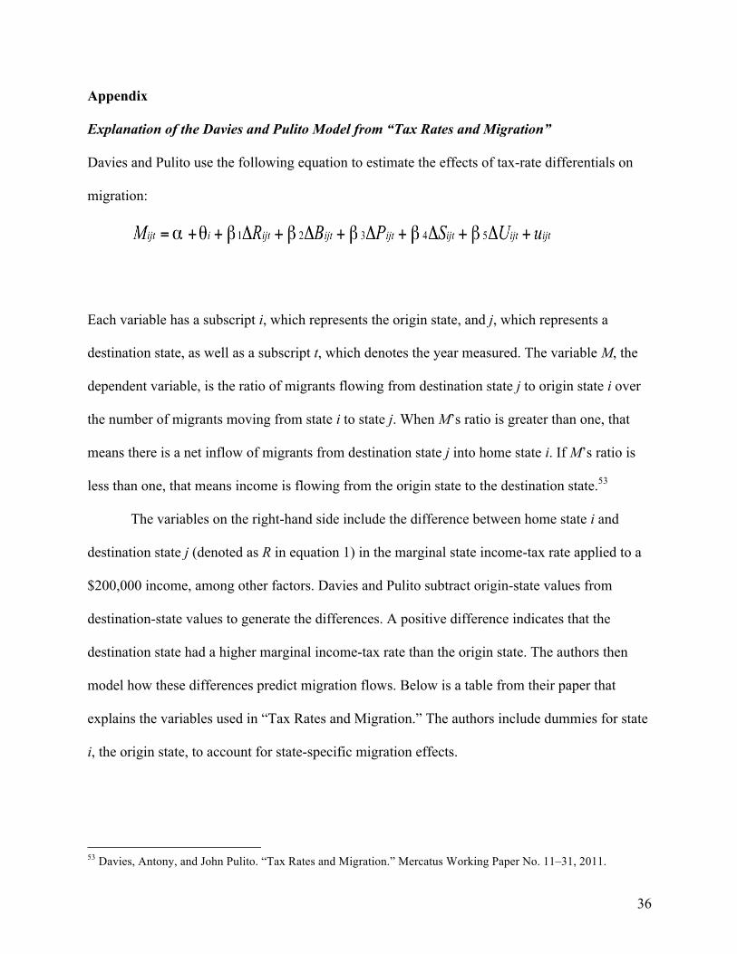
Explanation of the Davies and Pulito Model from “Tax Rates and Migration”

Davies and Pulito use the following equation to estimate the effects of tax-rate differentials on

migration:

Each variable has a subscript i, which represents the origin state, and j, which represents a

destination state, as well as a subscript t, which denotes the year measured. The variable M, the

dependent variable, is the ratio of migrants flowing from destination state j to origin state i over

the number of migrants moving from state i to state j. When M’s ratio is greater than one, that

means there is a net inflow of migrants from destination state j into home state i. If M’s ratio is

less than one, that means income is flowing from the origin state to the destination state.53

The variables on the right-hand side include the difference between home state i and

destination state j (denoted as R in equation 1) in the marginal state income-tax rate applied to a

$200,000 income, among other factors. Davies and Pulito subtract origin-state values from

destination-state values to generate the differences. A positive difference indicates that the

destination state had a higher marginal income-tax rate than the origin state. The authors then

model how these differences predict migration flows. Below is a table from their paper that

explains the variables used in “Tax Rates and Migration.” The authors include dummies for state

i, the origin state, to account for state-specific migration effects.

53 Davies, Antony, and John Pulito. “Tax Rates and Migration.” Mercatus Working Paper No. 11–31, 2011.

37

Appendix Figure 1

Davies and Pulito find that positive differences in tax rates, where state j’s rate was higher than

state i’s rate, were positively associated with migration into state i. The authors also find that

larger differences in income-tax rates were associated with larger amounts of migration.54

Results for Households and Individuals

This analysis originally began as a project to see how expense and tax burdens affect all three of

the IRS’s migration variables. In the end, I opted to focus on income migration to make this

analysis more tractable. Included in this appendix is the same set of regressions I ran for income

54 Davies, Antony, and John Pulito. “Tax Rates and Migration.” Mercatus Working Paper No. 11–31, 2011.

38

migration, only applied to returns and exemptions instead. The IRS tracks the migration of

returns, which approximate households, and exemptions, which approximate individuals.

Returns approximate households because individual returns cover dependent children and

married couples who file jointly. Exemptions approximate total population movement because

there is an exemption for each person on a tax return, such as a dependent child or a spouse,

making exemptions closely correlated with the number of individuals moving.55 The results are

extremely similar to the results for income migration in terms of sign and magnitude. They are

slightly more difficult to interpret, however, because the coefficients are so small, which in turn

is because the total net amount of households and individuals was divided by the population of

the origin state (i.e., the state households and individuals exited). Coefficients generally become

larger in magnitude as tax and expense burdens are lagged by more years, in regressions that

either compare levels to burdens or the natural log of income migration to burdens. Expense

burdens remain statistically significant at the 99 percent level throughout all regressions, while

the regressions of income migration on tax burdens are slightly less significant, especially as tax

burdens are lagged by more years.

55 See the Tax Foundation’s “Frequently Asked Questions about the Tax Foundation Migration Tool.” Available at http://interactive.taxfoundation.org/migration/FAQ.html.

39

Top 10 Return Migration Flows Between States, 2002–2010 Origin State Destination State Net Return Gain

1. New York Florida 131,767 2. California Arizona 78,107 3. California Nevada 73,461 4. California Texas 71,504 5. New Jersey Florida 64,675 6. New York New Jersey 63,000 7. California Oregon 49,406 8. New York North Carolina 44,449 9. Louisiana Texas 39,725 10. Michigan Florida 37,696

Appendix Figure 2

Top 10 Exemption Migration Flows Between States, 2002–2010 Origin State Destination State Net Exemption Gain

1. New York Florida 275,423 2. California Texas 205,977 3. California Arizona 186,911 4. New York New Jersey 163,899 5. California Nevada 155,991 6. New Jersey Florida 132,331 7. California Oregon 103,255 8. New York North Carolina 97,252 9. New York Pennsylvania 92,380 10. Louisiana Texas 88,984

Appendix Figure 3

40

Appendix Table 1

Regression Number 21 22 23 24 25VARIABLES Returns Returns Returns Returns Returns

L.ExpenseBurdenDifference -‐7.94e-‐06***(1.26e-‐06)

L2.ExpenseBurdenDifference -‐8.02e-‐06***(1.52e-‐06)




PopulationDifference 0*** 0*** 0*** 0*** 0***(0) (0) (0) (0) (0)

NaturalShareDifference -‐1.09e-‐06*** -‐1.15e-‐06*** -‐1.02e-‐06*** -‐8.93e-‐07*** -‐7.48e-‐07***(2.04e-‐07) (2.26e-‐07) (2.45e-‐07) (2.97e-‐07) (1.91e-‐07)

TaxBracketDifference -‐4.42e-‐06*** -‐4.47e-‐06*** -‐4.09e-‐06*** -‐3.99e-‐06*** -‐3.14e-‐06***(6.53e-‐07) (7.58e-‐07) (8.74e-‐07) (8.63e-‐07) (5.34e-‐07)

PersonalIncomeDifference 1.52e-‐09*** 1.55e-‐09** 1.51e-‐09** 8.40e-‐10 1.02e-‐09***(5.78e-‐10) (6.88e-‐10) (7.49e-‐10) (6.98e-‐10) (3.06e-‐10)

UnemploymentDifference -‐1.39e-‐05*** -‐1.44e-‐05*** -‐1.36e-‐05*** -‐1.16e-‐05*** -‐6.58e-‐06***(2.01e-‐06) (2.23e-‐06) (2.39e-‐06) (2.08e-‐06) (1.28e-‐06)

HispanicDifference 1.47e-‐07 5.43e-‐08 -‐1.79e-‐08 -‐2.06e-‐08 -‐4.00e-‐08(1.22e-‐07) (1.38e-‐07) (1.48e-‐07) (1.61e-‐07) (1.33e-‐07)

AfricanAmericanDifference -‐9.09e-‐07*** -‐8.29e-‐07*** -‐9.44e-‐07*** -‐6.35e-‐07*** -‐7.60e-‐07***(1.58e-‐07) (1.74e-‐07) (2.14e-‐07) (2.21e-‐07) (1.80e-‐07)

Over65Difference 1.45e-‐05*** 1.47e-‐05*** 1.24e-‐05*** 1.05e-‐05*** 8.72e-‐06***(1.86e-‐06) (2.16e-‐06) (2.39e-‐06) (2.27e-‐06) (1.99e-‐06)

JanuaryTemperatureDifference 2.17e-‐06*** 2.24e-‐06*** 2.24e-‐06*** 1.95e-‐06*** 1.35e-‐06***(2.68e-‐07) (3.13e-‐07) (3.62e-‐07) (3.23e-‐07) (2.49e-‐07)

CrimeDifference 1.08e-‐08*** 9.70e-‐09*** 1.05e-‐08*** 9.76e-‐09*** 9.56e-‐09***(2.21e-‐09) (2.89e-‐09) (3.15e-‐09) (2.30e-‐09) (1.97e-‐09)

Constant 1.33e-‐05 3.75e-‐05*** 5.36e-‐06 4.56e-‐05*** 5.13e-‐05***(8.61e-‐06) (1.19e-‐05) (1.07e-‐05) (9.49e-‐06) (9.61e-‐06)


Expense Burdens and Household Migration

41

Appendix Table 2

Regression Number 26 27 28 29 30VARIABLES Log Returns Log Returns Log Returns Log Returns Log Returns








TaxBracketDifference -‐0.0163*** -‐0.0128** -‐0.0118 -‐0.0160** -‐0.0184**(0.00579) (0.00631) (0.00716) (0.00812) (0.00908)


UnemploymentDifference -‐0.0743*** -‐0.0642*** -‐0.0622*** -‐0.0394** -‐0.0243(0.0148) (0.0153) (0.0160) (0.0176) (0.0192)

HispanicDifference 0.00368** 0.00489** 0.000743 -‐0.00193 -‐0.00185(0.00182) (0.00196) (0.00214) (0.00233) (0.00265)

AfricanAmericanDifference -‐0.00614*** -‐0.00202 -‐0.0106*** -‐0.0121*** -‐0.0142***(0.00234) (0.00252) (0.00285) (0.00318) (0.00359)

Over65Difference 0.0119 0.0107 -‐0.0170 -‐0.0292* -‐0.0455***(0.0107) (0.0114) (0.0132) (0.0150) (0.0173)



Constant -‐11.79*** -‐11.40*** -‐12.09*** -‐11.82*** -‐11.36***(0.182) (0.215) (0.219) (0.225) (0.250)


Expense Burdens and Log Household Migration

42

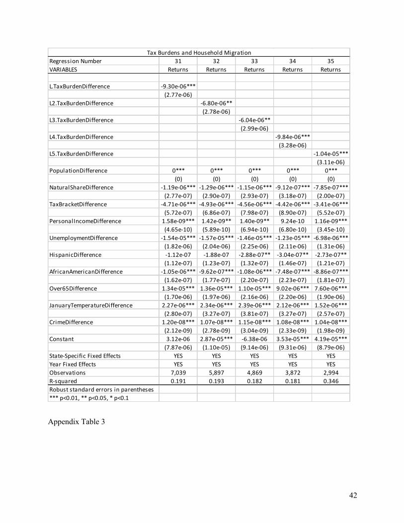
Appendix Table 3

Regression Number 31 32 33 34 35VARIABLES Returns Returns Returns Returns Returns

L.TaxBurdenDifference -‐9.30e-‐06***(2.77e-‐06)

L2.TaxBurdenDifference -‐6.80e-‐06**(2.78e-‐06)


L4.TaxBurdenDifference -‐9.84e-‐06***(3.28e-‐06)

L5.TaxBurdenDifference -‐1.04e-‐05***(3.11e-‐06)


NaturalShareDifference -‐1.19e-‐06*** -‐1.29e-‐06*** -‐1.15e-‐06*** -‐9.12e-‐07*** -‐7.85e-‐07***(2.77e-‐07) (2.90e-‐07) (2.93e-‐07) (3.18e-‐07) (2.00e-‐07)


PersonalIncomeDifference 1.58e-‐09*** 1.42e-‐09** 1.40e-‐09** 9.24e-‐10 1.16e-‐09***(4.65e-‐10) (5.89e-‐10) (6.94e-‐10) (6.80e-‐10) (3.45e-‐10)


HispanicDifference -‐1.12e-‐07 -‐1.88e-‐07 -‐2.88e-‐07** -‐3.04e-‐07** -‐2.73e-‐07**(1.12e-‐07) (1.23e-‐07) (1.32e-‐07) (1.46e-‐07) (1.21e-‐07)

AfricanAmericanDifference -‐1.05e-‐06*** -‐9.62e-‐07*** -‐1.08e-‐06*** -‐7.48e-‐07*** -‐8.86e-‐07***(1.62e-‐07) (1.77e-‐07) (2.20e-‐07) (2.23e-‐07) (1.81e-‐07)




Constant 3.12e-‐06 2.87e-‐05*** -‐6.38e-‐06 3.53e-‐05*** 4.19e-‐05***(7.87e-‐06) (1.10e-‐05) (9.14e-‐06) (9.31e-‐06) (8.79e-‐06)


Tax Burdens and Household Migration

43

Appendix Table 4

Regression Number 36 37 38 39 40VARIABLES Log Returns Log Returns Log Returns Log Returns Log Returns








TaxBracketDifference -‐0.0187*** -‐0.0165*** -‐0.0139* -‐0.0150* -‐0.0152(0.00583) (0.00638) (0.00725) (0.00820) (0.00926)



HispanicDifference -‐0.00153 -‐5.55e-‐05 -‐0.00464** -‐0.00683*** -‐0.00667***(0.00174) (0.00189) (0.00206) (0.00222) (0.00250)

AfricanAmericanDifference -‐0.00879*** -‐0.00443* -‐0.0131*** -‐0.0145*** -‐0.0175***(0.00232) (0.00250) (0.00283) (0.00316) (0.00352)

Over65Difference -‐0.00475 -‐0.00467 -‐0.0350*** -‐0.0426*** -‐0.0587***(0.0106) (0.0113) (0.0129) (0.0148) (0.0171)



Constant -‐11.98*** -‐11.55*** -‐12.28*** -‐11.94*** -‐11.53***(0.178) (0.210) (0.213) (0.219) (0.238)

Observations 7,039 5,897 4,869 3,872 2,994R-‐squared 0.358 0.384 0.387 0.407 0.399Robust standard errors in parentheses*** p<0.01, ** p<0.05, * p<0.1

Tax Burdens and Log Household Migration

44

Appendix Summary Statistics 1

Variable Observation Mean Standard Deviation Minimum MaximumNetReturnsPerCapita 10055 0.000054 0.0001357 4.39E-‐08 0.008124LogIncomeMigrationPerCapita 10055 -‐10.9607 1.589853 -‐16.9424 -‐4.81297ExpenseBurdenDifference 10055 -‐0.33075 1.559148 -‐5.68772 5.085021TaxBurdenDifference 10055 -‐0.16328 0.8017335 -‐3.88907 3.934228PopulationDifference 10055 -‐554908 9451724 -‐3.68E+07 3.67E+07NaturalShareDifference 10055 1.4146 7.412488 -‐35.5695 40.68332TaxBracketDifference 8938 -‐0.01992 3.986613 -‐10 10PersonalIncomeDifference 10055 -‐1709.14 7031.486 -‐26389 23261UnemploymentDifference 10055 -‐0.08221 1.608297 -‐9.6 7.1HispanicDifference 10055 1.792751 13.61622 -‐43.5862 44.32125AfricanAmericanDifference 10055 1.262274 13.57094 -‐36.4205 36.43007Over65Difference 8938 -‐0.33033 2.128296 -‐8.3955 8.488168JanuaryTemperatureDifference 8923 5.176734 15.21259 -‐52.3 55.1CrimeDifference 8937 457.6282 1184.294 -‐3275.7 4353.9

45

Appendix Table 5

Regression Number 41 42 43 44 45VARIABLES Individuals Individuals Individuals Individuals Individuals

L.ExpenseBurdenDifference -‐1.09e-‐05***(2.76e-‐06)






NaturalShareDifference -‐1.72e-‐06*** -‐1.79e-‐06*** -‐1.37e-‐06** -‐1.02e-‐06 -‐6.25e-‐07(4.51e-‐07) (5.01e-‐07) (5.60e-‐07) (7.46e-‐07) (4.04e-‐07)


PersonalIncomeDifference 2.60e-‐09* 3.12e-‐09* 2.58e-‐09 8.98e-‐10 1.82e-‐09**(1.43e-‐09) (1.63e-‐09) (1.81e-‐09) (1.75e-‐09) (7.43e-‐10)


HispanicDifference 3.40e-‐07 1.22e-‐07 2.20e-‐07 5.33e-‐08 7.15e-‐08(2.91e-‐07) (3.21e-‐07) (3.34e-‐07) (3.92e-‐07) (3.27e-‐07)

AfricanAmericanDifference -‐1.16e-‐06*** -‐1.02e-‐06** -‐8.65e-‐07* -‐2.68e-‐07 -‐5.06e-‐07(3.79e-‐07) (4.05e-‐07) (4.87e-‐07) (5.22e-‐07) (4.26e-‐07)



CrimeDifference 2.03e-‐08*** 1.81e-‐08*** 1.63e-‐08** 1.63e-‐08*** 1.44e-‐08***(5.18e-‐09) (6.67e-‐09) (6.83e-‐09) (6.02e-‐09) (4.58e-‐09)

Constant -‐1.28e-‐05 -‐1.47e-‐05 5.50e-‐06 1.18e-‐05 1.06e-‐05(2.48e-‐05) (2.82e-‐05) (3.29e-‐05) (3.70e-‐05) (2.96e-‐05)


Expense Burdens and Individual Migration

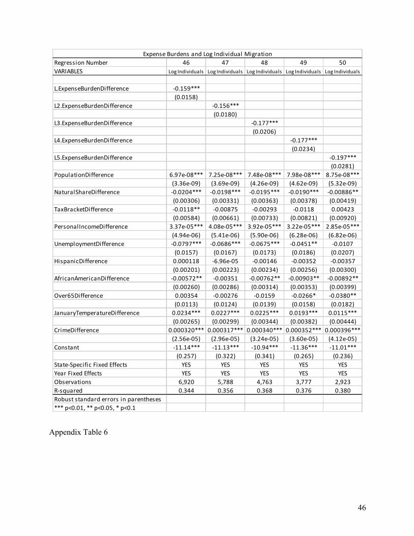
46

Appendix Table 6

Regression Number 46 47 48 49 50VARIABLES Log Individuals Log Individuals Log Individuals Log Individuals Log Individuals







NaturalShareDifference -‐0.0204*** -‐0.0198*** -‐0.0195*** -‐0.0190*** -‐0.00886**(0.00306) (0.00331) (0.00363) (0.00378) (0.00419)

TaxBracketDifference -‐0.0118** -‐0.00875 -‐0.00293 -‐0.0118 0.00423(0.00584) (0.00661) (0.00733) (0.00821) (0.00920)



HispanicDifference 0.000118 -‐6.96e-‐05 -‐0.00146 -‐0.00352 -‐0.00357(0.00201) (0.00223) (0.00234) (0.00256) (0.00300)

AfricanAmericanDifference -‐0.00572** -‐0.00351 -‐0.00762** -‐0.00903** -‐0.00892**(0.00260) (0.00286) (0.00314) (0.00353) (0.00399)

Over65Difference 0.00354 -‐0.00276 -‐0.0159 -‐0.0266* -‐0.0380**(0.0113) (0.0124) (0.0139) (0.0158) (0.0182)



Constant -‐11.14*** -‐11.13*** -‐10.94*** -‐11.36*** -‐11.01***(0.257) (0.322) (0.341) (0.265) (0.236)


Expense Burdens and Log Individual Migration

47

Appendix Table 7

Regression Number 51 52 53 54 55VARIABLES Individuals Individuals Individuals Individuals Individuals

L.TaxBurdenDifference -‐1.69e-‐05***(5.59e-‐06)


L3.TaxBurdenDifference -‐1.10e-‐05*(6.02e-‐06)




NaturalShareDifference -‐1.71e-‐06*** -‐1.89e-‐06*** -‐1.44e-‐06** -‐9.44e-‐07 -‐6.74e-‐07(5.99e-‐07) (6.36e-‐07) (6.87e-‐07) (7.94e-‐07) (4.16e-‐07)


PersonalIncomeDifference 3.03e-‐09** 3.25e-‐09** 2.76e-‐09* 1.46e-‐09 2.23e-‐09***(1.19e-‐09) (1.44e-‐09) (1.66e-‐09) (1.64e-‐09) (8.19e-‐10)


HispanicDifference -‐1.13e-‐08 -‐1.97e-‐07 -‐1.51e-‐07 -‐3.81e-‐07 -‐2.29e-‐07(2.74e-‐07) (2.90e-‐07) (3.12e-‐07) (3.44e-‐07) (2.98e-‐07)

AfricanAmericanDifference -‐1.32e-‐06*** -‐1.19e-‐06*** -‐1.04e-‐06** -‐4.32e-‐07 -‐6.67e-‐07(3.88e-‐07) (4.10e-‐07) (4.95e-‐07) (5.21e-‐07) (4.19e-‐07)




Constant -‐2.62e-‐05 -‐2.86e-‐05 -‐9.18e-‐06 -‐6.18e-‐06 -‐2.76e-‐06(2.30e-‐05) (2.58e-‐05) (2.97e-‐05) (3.78e-‐05) (2.88e-‐05)


Tax Burdens and Individual Migration

48

Appendix Table 8

Regression Number 56 57 58 59 60VARIABLES Log Individuals Log Individuals Log Individuals Log Individuals Log Individuals







NaturalShareDifference -‐0.0194*** -‐0.0189*** -‐0.0174*** -‐0.0141*** -‐0.00713*(0.00320) (0.00353) (0.00386) (0.00395) (0.00425)

TaxBracketDifference -‐0.0139** -‐0.0129* -‐0.00576 -‐0.0106 0.00653(0.00589) (0.00666) (0.00741) (0.00819) (0.00928)



HispanicDifference -‐0.00497*** -‐0.00485** -‐0.00679*** -‐0.00861*** -‐0.00861***(0.00192) (0.00214) (0.00225) (0.00247) (0.00290)

AfricanAmericanDifference -‐0.00800*** -‐0.00577** -‐0.00991*** -‐0.0112*** -‐0.0119***(0.00258) (0.00285) (0.00313) (0.00353) (0.00395)

Over65Difference -‐0.0102 -‐0.0172 -‐0.0334** -‐0.0382** -‐0.0500***(0.0111) (0.0124) (0.0138) (0.0155) (0.0180)



Constant -‐11.34*** -‐11.33*** -‐11.12*** -‐11.52*** -‐11.24***(0.251) (0.314) (0.333) (0.262) (0.211)


Tax Burdens and Log Individual Migration

49

Appendix Summary Statistics 2

Variable Observation Mean Standard Deviation Minimum MaximumNetExemptionsPerCapita 10117 0.000104 0.0002901 5.59E-‐08 0.018817LogIncomeMigrationPerCapita 10117 -‐10.335 1.595444 -‐16.7002 -‐3.97299ExpenseBurdenDifference 10117 -‐0.35735 1.55432 -‐5.68772 5.085021TaxBurdenDifference 10117 -‐0.17673 0.8000085 -‐3.88907 3.934228PopulationDifference 10117 -‐1017753 9392909 -‐3.68E+07 3.67E+07NaturalShareDifference 10117 1.525992 7.385788 -‐40.41 40.68332TaxBracketDifference 8996 0.09382 3.985031 -‐10 10PersonalIncomeDifference 10117 -‐2107.12 6919.179 -‐26389 22083UnemploymentDifference 10117 -‐0.12829 1.606842 -‐9.6 7.5HispanicDifference 10117 0.677722 13.69404 -‐43.5862 44.32125AfricanAmericanDifference 10117 0.96649 13.5945 -‐36.4205 36.43007Over65Difference 8996 -‐0.17301 2.146716 -‐8.3955 8.488168JanuaryTemperatureDifference 8981 4.633359 15.36633 -‐52.3 55.1CrimeDifference 8995 404.7195 1202.359 -‐4064 4353.9

mercatus graduate policy essay i would like to thank each of my mercatus graduate policy essay...

Documents