meta-analysis of tumour necrosis factor-alpha inhibitor treatment...
TRANSCRIPT

Meta-Analysis of Tumour NecrosisFactor-α Inhibitor Treatment for
Rheumatoid Arthritis
Christian Hollensen
Supervisors:Per Bruun Brockhoff, IMM, DTU
Rune Viig Overgaard, Biomodelling, Novo NordiskLene Alifrangis, Biomodelling, Novo Nordisk
Henning Bliddal, Parker Institute, Frederiksberg HospitalRobin Christensen, Parker Institute, Frederiksberg Hospital
Kongens Lyngby 2009IMM-MSC thesis-2009-19

Technical University of DenmarkInformatics and Mathematical ModellingBuilding 321, DK-2800 Kongens Lyngby, DenmarkPhone +45 45253351, Fax +45 [email protected]
IMM-MSC

Summary
Rheumatoid arthritis (RA) is a painful and disabling disease which affects 1 %of the general population. In the last decade new biologic disease-modifyingantirheumatic drugs (DMARDs) have emerged, which target specific cytokinesor cells, that are critical for the persistence of RA symptoms. Among thesebiologic drugs, three tumour necrosis factor-α (TNF-α) inhibitors called adali-mumab, etanercept, and infliximab have been the first to be applied in clinicalpractice. Though these three drugs target the same cytokine they differ bydosage, pharmacokinetic (PK) and pharmacodynamic (PD) properties. So farno meta-analyses of the drugs, which employ the efficacy time course of thesethree drugs or compare the efficacy of the drugs with their respective PK andPD properties, have ever been performed.A literature review was executed to find all double-blind randomised controlledtrials (DBRCTs) with the three TNF-α inhibitors. Numbers of responders ac-cording to the American College of Rheumatology(ACR) response criteria wereextracted from all the found publications concerning trials. A meta-analysis wasperformed on this data to acquire the typical efficacy progression of the threedrugs at different dosages. Nonlinear mixed-effects modelling was employed toestimate fixed parameters for the three treatments. A model with binomial dis-tributed error and random effects on trial level was chosen as a final model forthe ACR data.A PK-PD analysis was performed for the three drugs. This analysis was basedon PK data and PD parameters found from publications. Using this informa-tion, a 6-compartment PK-PD models was constructed for each of the threeTNF-α inhibitors. The PK-PD models concern the concentrations of TNF-α,its inhibitor, and their joint complex in the body when subjected to TNF-αtreatment by any of the three drugs. These models were used to simulate the

ii
typical TNF-α concentration in response to treatment with any of the threedrugs at the dosage levels seen in the DBRCTs.The final ACR model showed that there was a significant difference between theefficacy parameters of etanercept and the two other treatments, adalimumaband infliximab. Etanercept had a higher number of responders according to theparameters of the final model. Initiation of methotrexate (MTX) treatment wasshown to increase the number of responders. A termination of MTX treatmentdecreased the number of responders.The PK-PD model simulations displayed a concentration difference of free TNF-α between the three different drug treatments. The outcome of the PK-PD sim-ulations was compared with the parameters of ACR model. This comparisonshowed a semilogarithmic relationship between the maximal concentration offree TNF-α and the maximum proportion of responders during treatment withTNF-α inhibitors.Etanercept is the TNF-α treatment for RA with the highest proportion of re-sponders. This analysis shows that the number of responders is induced by thedosage and PD characteristics of the drug. The efficacy of a TNF-α treatmentis determined by its ability to persistently keep TNF-α concentration low.

Resume
Rheumatoid arthritis (RA), pa dansk kaldet kronisk leddegigt, er en smerte-fuld og invaliderende sygdom, som rammer 1 % af befolkningen. I løbet af detsidste arti er immunsupprimerende stoffer blevet introduceret i klinisk praktis,som er rettet mod specifikke cytokiner og celler, der er kritiske for fortsættelsenaf RA symptomer. De førstanvendte i klinisk praksis blandt disse biologiskestoffer er tre tumornekrotiserende faktor-α (TNF-α) hæmmere, kaldet adali-mumab, etanercept og infliximab. Selvom disse tre stoffer er rettet mod detsamme cytokin adskilles de af dosering, farmakokinetiske (PK) og farmakody-namiske (PD) egenskaber. Indtil nu er der hverken blevet lavet metaanalyser,som bruger den tidslige virkningsgrad af de tre stoffer eller som sammenlignervirkningsgraden for disse stoffer med deres respektive PK og PD egenskaber.Et systematisk litteraturstudie blev foretaget for at finde alle dobbelt-blinde ran-domiserede kontrollerede kliniske forsøg med de tre TNF-α hæmmere. Antal afrespondenter efter American College of Rheumatology (ACR) forbedrings kri-terier blev uddraget fra artiklerne om de kliniske forsøg. En meta-analyse blevudført pa disse data for at estimere det typiske virkningsforløb for de tre stoffer.Nonlinær mixed-effects modellering blev brugt til at estimere faste parametrefor de tre behandlinger. En model med binomialfordelte residualer og variansef-fekter mellem de forskellige kliniske forsøg blev valgt som den endelige modelfor ACR dataene.En PK-PD analyse for disse tre stoffer blev udført. Denne analyse var baseretpa PK data og PD parametre fra publikationer. Ved hjælp af disse infor-mationer blev 6-compartment PK-PD modeller konstrueret for hver af de treTNF-α hæmmere. PK-PD modellerne omhandler koncentrationen af TNF-α,dens hæmmer og deres fælles kompleks koncentration i kroppen, nar den bliverpavirket af TNF-α behandling fra de tre stoffer. Disse modeller blev brugt tilat simulere den typiske TNF-α koncentration ved behandling med de tre stoffer

iv
pa doseringerne, der blev set i de fundne kliniske forsøg.Den endelige ACR model viste, at der var en signifikant forskel mellem parame-trene for virkningsgraden af etanercept og de to andre behandlinger, adalimu-mab og infliximab. Etanercept havde en højere andel af respondenter ifølgeparametrene fra den endelige model. Pabegyndelse af behandling med metho-trexat(MTX) viste sig at forhøje antallet af respondenter. Afslutning af behan-dling med MTX viste sig at sænke antallet af respondenter.Simulationerne fra PK-PD modellerne viste en forskel i den frie koncentration afTNF-α mellem behandlingerne med de tre forskellige stoffer. Resultaterne fraPK-PD simulationerne blev sammenlignet med parametrene fra ACR modellen.Denne sammenligning viste et semilogaritmisk forhold mellem den maksimalekoncentration af frit TNF-α og den makisimale andel respondenter med TNF-αbehandling.Etanercept er den TNF-α behandling mod RA med den højeste proportionaf respondenter. Denne analyse viser at antallet af respondenter skyldes stof-fets doserings og PD egenskaber. Virkningsgraden af en TNF-α behandling erbestemt af dennes evne til vedvarende at holde TNF-α koncentrationen lav.

Preface
This thesis was conducted at the department of Informatics and MathematicalModelling (IMM) at the Technical University of Denmark (DTU) and at theBiomodelling department of Novo Nordisk in fulfillment of the requirements foracquiring the Master degree in engineering. The work started the 1st of October2009.
The thesis deals with a meta-analysis of TNF-α inhibitor treatment for rheuma-toid arthritis by using nonlinear mixed-effects models. As part of the thesis aliterature review has been performed and modelling with categorical and phar-macokinetic data.
Christian Hollensen Lyngby, 27th of March 2009

vi

Acknowledgements
I first and foremost wish to express my utter thanks to my supervisor Rune ViigOvergaard at the Biomodelling department of Novo Nordisk for his supervisionof this thesis. Our discussions, his overview of the modelling approach and hispatience for a biomedical student entering the world of modelling heightenedthe level of this thesis. Likewise I want to thank Lene Alifrangis for introducingme to world of pharmacokinetics and the help she provided for the constructionof the pharmacokinetic model.I want to express my sincere thanks to my supervisor Per Bruun Brockhofffor the theoretical feedback on the pragmatic approach of this thesis and forintroducing the linear and nonlinear modelling aspect as well as applicable ap-proaches for the thesis. I also want to thank the supervisors, Henning Bliddaland Robin Christensen, from the Parker Institute of Frederiksberg Hospital fortheir counselling regarding approaches and end points of the thesis to maintainthe clinical aspect.Furthermore I would like to thank for the help and comments I received fromthe rest of the wonderful people at the Biomodelling department at Bagsværd. Iwould also like to thank my fellow participants of the NLME course for our jointsessions and discussions about the theoretical and practical approaches to thenonlinear mixed-effects models, which helped me to get a better understandingof the tools of this thesis.At last I want to thank my fellow students at the biomedical programme, friendsand family for listening to my problems with the thesis, supporting me and en-couraging me to perform better whenever things got stuck.

viii

Abbreviations and symbols
Abbreviations
ACR American College of RheumatologyAPC Antibody-presenting cellDAS Disease activity scoreDBRCTs Double-blind randomised controlled trialsDMARD Disease-modifying antirheumatic drugDNA Deoxyribonucleic acidEU European UnionFOCE First order conditional estimateFDA Food and Drug administrationIFN-γ Interferon-γIgG Immunoglobulin GIL InterleukinITT Intended to treatITV Intertrial variationIV IntravenousMTX MethrotrexatemITT Modified intention to treatNLME Non linear mixed effects routineNONMEM Nonlinear mixed-effects modelNSAIDs Nonsteroidal anti-inflammatory drugsPD PharmacodynamicPK PharmacokineticRA Rheumatoid arthritisRefMan Reference Manager Professional Edition 11 c©
x Abbreviations and symbols
RSE Relative standard errorSC SubcutaneousTB TuberculosisTNF-α Tumour necrosis factor-αWOS Web of Science
Mathematical symbols
α Level of significance, the probability of making a type 1 errorβ Fixed parameter of a functionχ2 Chi square distributionε Error of a functionγ Gradient parameter of the efficacy functionΛ Likelihood ratioΩ Covariance matrix of random effectsσ2b Variance of the random effects
Σ Covariance matrix of the errorσ2 Variance of the errorΘ Parameter space of a modelθ Parameter of a model
A0 Amount of drug injectedAi Amount of drug in compartment ib Random parametersof a functionCi Concentration of the ith compartmentCl Clearance rate of the drugEmax Maximal efficacy parameter of the efficacy function.EL Elimination rate of TNF-αf(·) Model function.Ka First order absorption rate constantKoff Dissociation rate of the TNF-α and its inhibitor complexKon Association rate of the NF-α and its inhibitorH0 Hypothesis of the likelihood ratio testp(·) Probability functionProd Production rate of TNF-αQ Rate of transfer between the central and peripheral compartmentr Number of parameters in the model of H1
s Number of parameters in the model of H0
ti Sampling time of ith measurementT 1
2Time to achieve half of maximal efficacy
Tol Tolerance parameter of the efficacy functionVi Volume of the ith compartmentx Input of a function

xi
y Output of a functionwres Weighted residual
In this thesis bold font of a mathematical symbol indicates that the currentvariable represents more than a single value. This can be a group of values orall values within the variable, given either in one or several vector or matrices.

xii

Contents
Summary i
Resume iii
Preface v
Acknowledgements vii
Abbreviations and symbols ix
1 Introduction 1
2 Medical theory 32.1 Articulations of the body . . . . . . . . . . . . . . . . . . . . . . 42.2 The Inflammatory Response . . . . . . . . . . . . . . . . . . . . . 62.3 Rheumatoid Arthritis . . . . . . . . . . . . . . . . . . . . . . . . 82.4 Treatment of rheumatoid arthritis . . . . . . . . . . . . . . . . . 11
3 Mathematical Theory 153.1 Mathematical Modelling . . . . . . . . . . . . . . . . . . . . . . . 153.2 Nonlinear Modelling . . . . . . . . . . . . . . . . . . . . . . . . . 163.3 Pharmacokinetic Modelling . . . . . . . . . . . . . . . . . . . . . 183.4 Pharmacodynamic Modelling . . . . . . . . . . . . . . . . . . . . 20
4 Materials 234.1 S-plus . . . . . . . . . . . . . . . . . . . . . . . . . . . . . . . . . 234.2 NONMEM . . . . . . . . . . . . . . . . . . . . . . . . . . . . . . 24
5 Methods 27

xiv CONTENTS
5.1 Literature Review . . . . . . . . . . . . . . . . . . . . . . . . . . 275.2 Meta-Analysis . . . . . . . . . . . . . . . . . . . . . . . . . . . . . 315.3 Pharmacokinetic-Dynamic Modelling . . . . . . . . . . . . . . . . 37
6 Results 416.1 Literature Review . . . . . . . . . . . . . . . . . . . . . . . . . . 416.2 Meta-Analysis . . . . . . . . . . . . . . . . . . . . . . . . . . . . . 446.3 Pharmacokinetic-Dynamic Modelling . . . . . . . . . . . . . . . . 58
7 Discussion 657.1 Literature review . . . . . . . . . . . . . . . . . . . . . . . . . . . 657.2 Meta-analysis . . . . . . . . . . . . . . . . . . . . . . . . . . . . . 687.3 Pharmacokinetic-Dynamic modelling . . . . . . . . . . . . . . . . 71
8 Conclusion 75
A Numerical Estimation Approaches 77A.1 S-plus . . . . . . . . . . . . . . . . . . . . . . . . . . . . . . . . . 78A.2 NONMEM . . . . . . . . . . . . . . . . . . . . . . . . . . . . . . 80
B Trial Descriptions 85
C Trial Data 89
D Modelling Log 97
E Assumption Tests 105
F PKPD-results 121

Chapter 1
Introduction
Rheumatoid arthritis (RA) is a chronic and systemic inflammatory disordermainly involving the joints. It has a broad range of clinical features includingpain, stiffness and joint swelling[63]. The disorder has a prevalence of 1 % in thegeneral population and the main age of onset occurs in the age of 20-40 years[88].Beyond the disabling and painful effects of the disorder, RA patients also sufferfrom mortality rates of 1.5 fold higher than in the general population[96] andeven worse if untreated[24]. This is mainly due to physical disabilities and thesystemic complications arising from RA.
The typical medical treatment consists of disease-modifying antirheumatic drugs(DMARDs), nonsteroidal anti-inflammatory drugs (NSAIDs) and corticosteroidsto ensure remission of symptoms[77].
In the last decade biologic DMARDs has been approved for treatment of RA[94].Three inhibitors of the cytokine tumour necrosis factor-α (TNF-α), adalimu-mab, etanercept, and infliximab, belong to this group of drugs. They have beenthe treatment of choice to RA when the initial non-biologic DMARD treatmenthas proved insufficient[85].
Several systematic reviews have been performed on this area addressing the ef-ficacy of these approved TNF-α inhibitors in clinical trials [46][60][75]. Theseanalyses have all been occupied with trial end points or efficacy at a given timebut not the time course of efficacy proportions.
Improvements in knowledge management and decision-making have been achieved

2 Introduction
in the industrial drug development by the use of mathematical modelling thatmake use of the time course of drug responses[61]. Since these advanced meth-ods are applicable and efficient in the drug development phase, they should alsobe applicable and efficient in the analysis of clinical trials. Mathematical modelsthat incorporate data from clinical trials may be constructed. These mathema-tical models would support the decisions of physicians on which drug to use,which dosing regimen to follow with respect to a specific patient and which con-comitant treatment to choose. They could also support the decision-making onthe duration of a drug treatment without improvements in patient state beforeshifting to another treatment.In this thesis a nonlinear mixed-effects modelling approach is used in a meta-analysis to estimate the efficacy time course of the three TNF-α inhibitors,adalimumab, etanercept, and infliximab. The meta-analysis is based upon ef-ficacy data from publications concerning double-blind randomised controlledtrials (DBRCT). The purpose of the meta-analysis is to identify differences bet-ween the the TNF-α inhibitor treatments.These three drugs target the same cytokine, but are different with respect to e.g.dosing regimen, half life in the body and affinity. Therefore a pharmacokinetic(PK) and pharmacodynamic (PD) analysis of these three drugs is performedon the basis of publicised results. The results of this analysis will be used tosubstantiate the results of the meta-analysis as well as hypothesize about therelationship between the concentration of TNF-α in the blood and disease re-mission.

Chapter 2
Medical theory
This chapter explains the basic medical theory to understand the purpose andresults of the analysis. An overview concerning the physiology and anatomy ofthe articulations of the body with emphasis on the synovial joint is summarisedin the first section. In the next section, the general inflammatory response andits mechanisms in the human body are described. The existing knowledge of RAis then described in the following section with main emphasis on the cytokineTNF-α. Parts of this section requires some knowledge of the physiological sys-tems involved. In the last section of the chapter treatment of the disease isexplained along with staging of remission.
The first physiological section has been written on the basis of [34] and [89].The main part of the following patophysiological sections has been written onthe basis of [76] and [88].
Readers familiar with the physiology of the human body can skip the first twosections without losing a perspective of the rest of the thesis. Readers with ex-perience and extensive knowledge about the treatment and mechanisms of RAshould be able to skip the whole chapter.
4 Medical theory
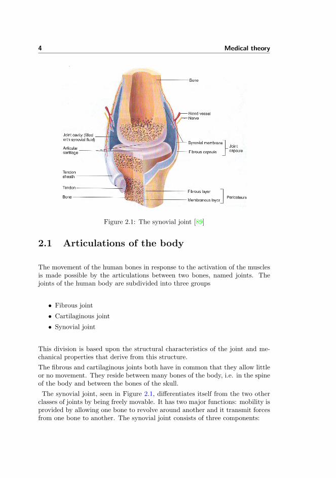
Figure 2.1: The synovial joint [89]
2.1 Articulations of the body
The movement of the human bones in response to the activation of the musclesis made possible by the articulations between two bones, named joints. Thejoints of the human body are subdivided into three groups
• Fibrous joint
• Cartilaginous joint
• Synovial joint
This division is based upon the structural characteristics of the joint and me-chanical properties that derive from this structure.
The fibrous and cartilaginous joints both have in common that they allow littleor no movement. They reside between many bones of the body, i.e. in the spineof the body and between the bones of the skull.
The synovial joint, seen in Figure 2.1, differentiates itself from the two otherclasses of joints by being freely movable. It has two major functions: mobility isprovided by allowing one bone to revolve around another and it transmit forcesfrom one bone to another. The synovial joint consists of three components:

2.1 Articulations of the body 5
• The articular cartilage
• The synovial fluid
• The joint capsule
The articular cartilage covers the ends of both bones of the joint. The articularcartilage consists 65-85 % water, which is quite a lot considering the workloadthe tissue can carry. This is compared to the bones of the human body whichconsists of 20 % water. The extracellular matrix of the tissue consists of a densenetwork of collagen fibrils in a concentrated solution of proteoglycans. Thechondrocytes, which are the main cells of the tissue, constitute about 10 % ofthe articular cartilage volume. There are only blood vessels in the peripheralmargins of the articular cartilage so the chondrocytes are dependent upon nu-trition from the underlying bone and the synovial fluid.
The collagen fibrils, proteoglycans, and water determine the viscoelastic materialcharacter of the tissue. Viscoelastic material changes its mechanical behaviorover time when subjected to constant load or constant deformation. This en-sures that the shape can be altered to ensure better contact in the joint.
The articular cartilage covering each of the two bones of the joint are covered bya thin layer of lubrication. This lubrication minimises friction even when loadsare high across the joint and provides a force that holds the articular cartilagecovering both bones together when the loads across the joints are low and car-tilage surfaces move quickly relative to each other. The lubrication force can becompared to the cohesion forces that hold together two pieces of glass when theircontact surface is covered with a thin layer of water. The cracking sounds of thejoints, that some individuals can produce when pulling their fingers, emergeswhen the cohesion force is no longer capable of holding the articular cartilagetogether and contact is lacking for a moment.
Like many of the other tissues of the body, articular cartilage is also able tomodify its character and mechanical properties in response to prolonged wearand tear. Physically active individuals tend to have thicker articular cartilagesand the thickness increases when the individual joint goes from generally inac-tive to an active state. The articular cartilage of some of the joints are alsospecialised to sustain greater loads developing intra-articular disks that enlargethe contact areas, as it is seen in the temporomandibular and knee joints.
The synovial fluid fills up the cavity of the joint. It is a complex mixture ofpolysaccharides, proteins, fat, and cells. The polysaccharides provide much ofthe slippery consistency and lubricating qualities of synovial fluid.
The joint capsule consists of two layers. The outer layer is the fibrous capsulewhich consists of dense irregular connective tissue. It is attached to the fibrouslayer of the periosteum of the bones of the joint. The capsule can thicken toform ligaments that restrict mobility of the joint as well as stabilising the joint.

6 Medical theory
This effect can also be provided and supported by ligaments and tendons out-side the fibrous capsule. The inner layer is called the synovial membrane andit covers all surfaces inside the joint cavity except the articular cartilage. Themain quality of the synovial membrane is to secrete constituents of the synovialfluid. Blood vessels and sensory nerves enter the joint capsule but never enterthe cavity of the joints. These blood vessels provide nourishments to the jointcapsule. The sensory nerves only enter the synovial membrane to a lesser extentand they supply information to the brain about physical harm in the joint aswell as information about the position and movements of the joint.As described the synovial joint is an interdependent system. The disorder ofone component can disturb the function of the whole system.
2.2 The Inflammatory Response
The inflammatory response comes as a reaction on harm or a breach on someof the defenses of the body. Inflammation can appear in the body as a red-ness(rubor), heat(calor), swelling(tumor), pain (dolor), and loss of function(function laesa). The acute inflammatory response arise as a response to tissueinjury that ranges from mechanical harms as blisters, bruises, and broken bonesto the injuries that arises when pathologic particles and organisms enter thebody. The inflammatory response is complex and includes many different andcorrelated elements which serve to destroy the source of injury, remove accumu-lated debris and trigger the repair process.Acute inflammation consists of two components: vascular and cellular response,illustrated i Figure 2.2. The vascular response serves to increase the blood flowof the subjected tissue. It arises from the initial fleeting constriction of the arte-rioles and precapillary sphincters reducing vascular resistance and dilating thearterioles. At the same time cytokines and other inflammatory specific proteinscause the endothelial cells of the capillaries of the injured tissue to contractslightly allowing greater permeability into the tissue.This allows the formation of exudate, a fluid containing plasma proteins thatnormally only resides in the blood vessels, which passes into the injured tissueat an increased rate. The formation of exudate disturbs the normal osmoticpressure between blood vessels and the tissue allowing accumulation of fluid inthe injured tissue producing the earlier mentioned swelling. The blood becomesmore viscous as volume drops which in turn induces the red blood cells to aggre-gate increasing viscosity even more. This reduces the blood flow and can inducetemporary cessation of blood flow. This is a general description of the vascularresponse, the intensity of the injury determines the amount of tissue affected,exudate created, and time length of the response. The vascular component hasfour benefits:

2.2 The Inflammatory Response 7
Figure 2.2: The acute inflammatory response.
• Dilution of toxins. Decreases their damage on the tissue.
• Pain from swelling. Limits movement and prevents further damage.
• Presence of antibodies and proteins in the tissue. Act against disease-causing microorganisms.
• Amplifies the cellular response. Increases migration of white blood cellsinto the tissue and increases their activity in the tissue.
The cellular component starts initially with the aggregation of the red bloodcells described above. The aggregation of red blood cells has mainly two effects:
• The aggregated red blood cells are now the largest units in the bloodoccupying the center of the vessels and forcing the white blood cells, orleukocytes, to assume a peripheral position in the blood, the margination.
• The blood flow is slowed in the vessels allowing the leukocytes to adhere tothe endothelial cell wall and begin transmigration into the inflamed tissue.
The cellular response comes in waves of two types of cells. The first cells dom-inating the scene are the polymorphonuclear cells, mostly neutrophils, non-specific immune cells, which are most numerous in the first 6-24 hours, thenlater outnumbered by the mononuclear cells, e.g. macrophages. The cells begindigesting particles, a process called phagocytosis. The cells are directed by thehelp of the chemical constituents of the inflamed tissue. When the cell recog-nises a pathogen particle it engulfs the target and degrades the particles by thehelp of self produced enzymes and free radicals. The cellular response changesdepending on the source and grade of injury, summoning different types of cellsin response to specific injuries and breaches of the body’s natural barriers.

8 Medical theory
In the case that the acute inflammatory response does not remove the sourceof injury the inflammation may become chronic. This can be due to a standoffbetween the injurious agent and the defenses of the body or a malfunction in theimmune system, which causes the body to attack healthy cells. In this phase thecellular response is governed by a class of cells called lymphocytes. These cellsrelease lymphokines which effect macrophages and the inflammatory responsecontinues.
2.3 Rheumatoid Arthritis
The mechanisms of action in RA have not been fully disclosed. The disease hasbeen classified as a chronic systematic disease with prominent involvement ofthe joints [76]. It seems to be caused by genetic, infectious and environmentalelements in interrelated ways [30][92]. It affects 1 % of the population in theindustrialised world primarily with onset in the age of 20-40 years, in a femaleto male ratio of 3:1[88] and can lead to 1.5 fold in mortality rate[96].The typical clinical picture of the disease is a chronic inflammation that grad-ually increases, which causes swelling and pain in the distal joints, primarilyof the wrists, hands, ankles and feet as well as the larger joints in shouldersand knees. The disease has a varied time course from patient to patient. Somepatients experience an aggressive onset in many joints others develop extra-articular manifestations in the heart, lungs, skin and other organs[88]. Thediagnostic criteria for the disease include
- Presence of morning stiffness,
- Arthritis of at least 3 joint areas
- Arthritis of the hand joints
- Symmetric arthritis
• Rheumatoid nodules
• Elevated levels of serum rheumatoid factor
• Radiographic changes
The first four criteria should have persisted for at least 6 six weeks and thepatient should have at least four of the seven the criteria for a RA diagnosis[77].The current hypothesis of initiation involves the lymphocytes known as B andT cells[25][92][94], but no specific extrinsic or intrinsic factor that activate thesecells have been identified. It is believed that these undefined factors are pre-sented to the immune cells by some antibody presenting cell (APC). Caucasians

2.3 Rheumatoid Arthritis 9
Figure 2.3: The current understanding of rheumatoid arthitis adapted from [94].In the figure synovial tissue is a collective term for both the synovial fluid andmembrane, since most of the reaction takes place in both compartments. APC:Antibody presenting cell. IL: Interleukin. TNF: Tumour necrosis factor. IFNγ:Interferon-γ.
of the HLA-DR4 genotype has 3.5 times greater risk of developing RA than cau-casians of other DR genotypes, whereas RA is connected with other genotypesin other populations[92]. But the fact is that activated B and T cells are presentin the synovial membrane of the joint.
The T cells maintains and stimulates the inflammation by secreting lymphokinesas TNF-α, interleukin(IL)-2 and interferon-γ (IFN-γ), see Figure 2.3. Thesecytokines induce activation of the B cells, macrophages, fibroblasts and osteo-clasts.
The B-cells differentiate into plasma cells that secrete rheumatoid factor andother autoantibodies, which reinforces the inflammation by activating T cellsand increases the production of TNF-α[92][94].
The macrophages produce additional cytokines, as TNF-α, IL-1 and IL-6, which

10 Medical theory
activates various cell populations. These inflammatory responses and other ef-fects contribute to an increase of synovial fluid and a thickening of the synovialmembrane, it becomes irregular and develops fingerlike projections into the jointcavity, the so-called pannus. The activated synovial fibroblasts secrete matrixmetalloproteinases which initiates irreversible erosion and destruction of artic-ular cartilage and assists in bone destruction. The osteoclasts of the underlyingjoint bone are the main source of irreversible bone degradation when activatedand they also differentiate in the synovial membrane[94].
2.3.1 TNF-α
TNF-α is produced primarily by T cells, monocytes, and macrophages. TNF-αis secreted by one of these cells when exposed to either pathogens to Toll-likereceptor, or cytokines, IL-1 or TNF-α, to cytokine receptors. These receptorsboth reside at the outside of the cell membrane. This stimulates a sequence ofevents leading to the transcription of the TNF-α gene. TNF-α is expressed as amembrane-bound protein that self-associates into its bioactive homotrimmer. Itis released from the membrane by the TNF-α converting enzyme. In its trimericform it can activate the TNF receptors, TNFR1 and TNFR2, both when solubleand transmembrane.
Activation of TNFR1 can induce apoptosis, automated cell death, as well asblocking apoptosis, inducing cell proliferation, and production of proinflamma-tory proteins at the same time[91]. The effect of TNFR1 activation is dependenton the type of cell and simultaneous stimuli. Cell to cell contact is required toactivate TNFR2 which is only situated on immune and endothelial cells. The ac-tivation of TNFR2 cannot induce apoptosis but only the same proinflammatoryresponse as the TNFR1 receptor.
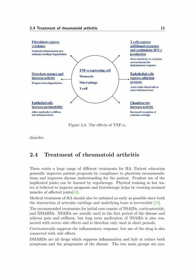
Exposure to TNF-α also induces different results on different cells in vitro, seeFigure 2.4. Fibroblasts express IL-6[113] and matrix metalloproteinases[94].Endothelial cells express adhesion proteins[17]. T cells expresses TNF-receptorsand high affinity IL-2 receptors while costimulating IL-2 dependent IFN-γ pro-duction [86]. Osteoclast precursors differentiate into mature osteoclasts[19].Chondrocytes increases resorption of articular cartilage[22]. Epithelial cells in-creases permeability [73]. Some of the effects have been proved to be concen-tration dependent and inhibited by an anti-TNF-α inhibitor[35][73].
As it can be seen TNF-α induces proinflammatory stimuli in many cells andhas a positive feedback upon itself which signifies its importance in the chronicinflammatory mechanisms of RA. It is possible to perceive that the TNF-α is avital part of the immune defense system of the body. With the many interac-tions of TNF-α in RA it is an important cytokine to inhibit in order to halt the
2.4 Treatment of rheumatoid arthritis 11
Figure 2.4: The effects of TNF-α.
disorder.
2.4 Treatment of rheumatoid arthritis
There exists a large range of different treatments for RA. Patient educationgenerally improves patient prognosis by compliance to physician recommenda-tions and improves disease understanding for the patient. Prudent use of theimplicated joints can be learned by ergotherapy. Physical training in hot wa-ter is believed to improve prognosis and fysiotherapy helps by treating strainedmuscles of affected joints[88].Medical treatment of RA should also be initiated as early as possible since boththe destruction of articular cartilage and underlying bone is irreversible [76].The recommended treatments for initial care consist of NSAIDs, corticosteroids,and DMARDs. NSAIDs are usually used in the first period of the disease andrelieves pain and stiffness, but long term medication of NSAIDs is also con-nected with severe side effects and is therefore only used in short periods.Corticosteroids suppress the inflammatory response, but use of the drug is alsoconnected with side effects.DMARDs are all drugs which suppress inflammation and halt or reduce bothsymptoms and the progression of the disease. The two main groups are syn-

12 Medical theory
thetic DMARDs, which for have been on the market for over half a century, andbiologic, which have been introduced over the last two decades.Methotrexate (MTX) is the synthetic DMARD, which has been identified as themost successful to induce a long-term response[77]. MTX has effect on DNA-synthesis and on the cascade of events initiated by IL-1, IL-6 and TNF-α[90]reducing the inflammatory response.The armatory against RA has been upgraded with new biologic DMARDs thattarget cytokines or cells, which have been identified as critical for the persis-tence of RA symptoms. These drugs are either monoclonal antibodies or fusionproteins that are either chimeric or human[100]. They have revolutionised thetreatment possibilities of patients in which traditional drugs had showed noprogress.If structural damage of the joints continues and all possible drug treatmentsfail, surgery is the last possible resolution [77]. The affected parts of the jointare surgically removed and are replaced by alloplastic [88].Efficacy of the treatment should be regularly assessed and patients should bemade aware of side effects to achieve remission or lowering disease activity.Treatment by combination of different drugs is recommended if patients are notshowing any progress to monotherapy[77].
2.4.1 TNF-α inhibitors
TNF-α inhibitors are part of the new biologic DMARD armatory that has beenclinically introduced during the last 15 years. The drugs bind to soluble andmembrane-bound TNF-α molecules to form a complex. This complex is hin-dered from binding with receptors, thus stopping the proinflammatory effects ofTNF-α mentioned above. These drugs were the first efficient biologic DMARDsintroduced and therefore they remain the first line of response when conven-tional treatment has failed. The three commercially released TNF-α inhibitorsare Infliximab, Etanercept, and Adalimumab respectively sold under the namesRemicade, Enbrel and Humira.Adalimumab is a human immunoglobulin G (IgG)1κ monoclonal antibody. Itis produced in an mammalian cell expression system and has an approximatemolecular weight of 148 kiloDalton (kDa)[4]. It has been shown to penetrate themembrane of TNF-α expressing cells in vitro when in the presence of comple-ment. The recommended dose of 40 mg is given every other week subcutaneous(SC), meaning that it can be self-injected by a patient if a physician deems itappropriate[10]. MTX treatment is recommended to be continued if it was theprior treatment. It was approved for use against RA in December 2002 by theFood and Drug Administration (FDA) in the US and in September 2003 by theEuropean Union (EU)[9].

2.4 Treatment of rheumatoid arthritis 13
Etanercept is a fusion protein consisting of the human TNFR linked with thehuman IgG1 antibody. It is produced in a mammalian cell expression systemand has an approximate molecular weight of 150 kDa[3]. The recommended doseof 25 mg is given SC twice a week[6]. It was approved for human use againstRA in November 1998 by the FDA and in February 2000 by the EU[8].
Infliximab is a chimeric IgG1κ monoclonal antibody, which means that theantibody consists of both mouse and human regions. It is produced by a recom-binant cell line and has an approximate molecular weight of 149 kDa[2]. Therecommended dose of 3 mg/kg is given intravenously (IV) over 2 hours. Therecommended dosage is given at week 0, 2, 6, and every 8th week after that[5].It is recommended to use the drug in combination with MTX.
MTX has been shown to alter the PK properties of infliximab[68]. In case ofan unsatisfactory response the dose can be increased as far as 10 mg/kg ortreatment every fourth week. It was approved for human use against RA inNovember 1999 by the FDA and in August 1999 by the EU[7].
However there also complications associated with treatment of RA with TNF-αinhibitors. TNF-α is a general inflammatory cytokine, which also works in re-sponse to other diseases. Therefore the treatment decreases the normal responseto diseases. Patients treated with TNF-α inhibitors have increased propensityto tuberculosis(TB) and latent TB can be reactivated as a response to thetreatment. The incidence differs between the drugs, 54 versus 28 incidences per100.000 treated with infliximab and etanercept respectively[40]. Similar stu-dies concerning adalimumab has not been found by the author. Screening ofTB is therefore highly recommended before initiating treatment with TNF-αinhibitors. TNF-α inhibitors also increase the risk of other opportunistic infec-tions, meaning infections that would be warded by the normal immune defense.
Increased risk of health related events have been spotted at RA patients treatedwith these drugs compared to the normal RA population. These events includecardiovascular, pulmonary, liver, and neurological systems of the body. Pa-tients are also advised to use birth control when using these drugs because ofthe unknown side effects upon the foetus. Autoimmune-like syndromes as wellas anti nuclear antibodies have also been observed in patients receiving TNF-αinhibitor treatment[39].
The system of these events following treatment is not fully understood. As withmost drugs, the meddling of the physiological systems does not always comewithout a cost. The treatment with TNF-α inhibitors should be a carefullyconsidered and discontinuation should be revised when experiencing adverseevents or no improvement.
14 Medical theory
2.4.2 American College of Rheumatology efficacy measure
The concept of making randomised controlled trials is both to supervise thenumber of adverse events from a drug compared with the control treatment,either placebo or some already recognised treatment, and to ascertain the effi-cacy of the drug compared to the control treatment. To compare drugs used fora certain disease, it is important to specify a common efficacy measure that isused in all trials of a certain disease.In RA the most widespread efficacy measure is the definition given by the Amer-ican College of Rheumatology (ACR), the ACR response. The disease activityof the patient is measured in 7 ways:
- Number of tender joints.
- Number of swollen joints.
• Subjective assessment of pain by patient on visual analog scale.
• Subjective assessment of disease activity by patient on visual analog scale.
• Subjective assessment of disability by patient by using a health assessmentquestionaire.
• Subjective assessment of disease activity by the physician on a visual ana-log scale.
• Measurement of acute phase (Westergren erythrocyte sedimentation rate,rheumatoid factor or C-reactive protein level).
The ACR response is then set at 4 levels; 0, 20, 50, and 70 % improvement sincetreatment initiation. This proportional improvement is only required in thetender and swollen joint count, in the remaining measures only a proportionalimprovement in 3 out of 5 measures is required to acquire an ACR20, -50 or -70response[36][37].The FDA proposes a primary endpoint of phase III trials with RA to be aproportional comparison of patients with an ACR20 response at 6 months [1].Over the last 10 years there has developed a discussion among practitionersand analysers of RA trials whether the 50 or 70 % improvement measures arebetter to discriminate between drugs efficacies [26][38]. This partly reflects therevolution in the treatment of RA over the decade, which enables patients toacquire partly or fully remission in far greater proportions.There exists alternative efficacy measures of RA which includes disease activityscore (DAS) on 28 joints and the Sharp score. These are both expressed on acontinuous scale, but are not given as often in publications concerning DBRCT.

Chapter 3
Mathematical Theory
This chapter serves to give a conceptual and general understanding of the ma-thematical methods used to create the results of this thesis. The subject ofnonlinear mixed-effects modelling is immense and outside the scope of this the-sis. For a broader and more profound understanding of the nonlinear methodsconsult the works [13] and [29] from which the section has been inspired.
In the first section the concept of mathematical modelling is briefly introduced.In the second section nonlinear modelling is conceptually explained along withits binomial distribution extension. In the last sections, the concept and tech-nique of PK and PD modelling are explained. For a thorough understandingof these two subjects the author would like to refer to [42], which has been theinspiration of the sections.
3.1 Mathematical Modelling
The concept of mathematical modelling is broad and is used in a vast amountof areas. Mathematical models provide an excellent way of quantifying the ty-pical effects and their variations, as they are seen in everyday life. It also allowsscientists and practitioners to predict new data, within the framework of themodel, but outside the current available data. The common man experience

16 Mathematical Theory
models in his everyday life, when the weather for the next 5 days is predictedby the use of mathematical models.
Certain limitations exist for mathematical modelling. They will never be betterthan the data or parameters on which they are based. E.g. a PK model basedon data from pigs can be useful to predict the concentrational behaviour of adrug in humans, but the exact concentration is associated with large uncertain-ties.
The mathematical model is always built around the behaviour of the data andthe current knowledge about the system, which one requests to model. Equa-tions are set up with parameters that govern the dynamics of the model. Basedupon the knowledge and inferences about the system it is possible to set para-meters to values deduced from earlier experiments. It is also possible to estimatethem on the basis of currently available data.
Validating the model is an important step when the model is finished. Oneshould inspect that
• The mathematical assumptions of the model are not violated.
• The values of the model parameter values or model structure are not inviolation of the physical system.
• Compare predictions or simulations of the system to data from experi-ments.
If these inspections are adequately met, the model should be ready to use forany purpose within the framework of the model.
3.2 Nonlinear Modelling
The nonlinear model evolves around a very general equation
y = f(x,β) + ε, (3.1)
where y is the outcome of a measurement, f(·) is a nonlinear function governedby the input x, which describes the situation under which the measurement wastaken, e.g. time or temperature, and β is the fixed parameters of the function.ε is an error upon every measurement which is assumed normally distributedwith a mean value of 0. It is further assumed that the errors are independent,

3.2 Nonlinear Modelling 17
uncorrelated, have a common variance, and are identically distributed for allvalues of x. The system could be based upon input, output, and parametersconsisting of single values, vectors, or matrices.This is a general set-up of the nonlinear model which can be modified to suitthe system to be modelled. The nonlinear function gives the possibility ofconstructing a mechanistic model with more interpretability, parsimony, andvalidity beyond the observed range of the data[79].When an adequate function is found, the fixed parameters, β, can be estimatedusing an iterative numerical approach. Usually β is found by minimizing
(y− f(x,β))2, (3.2)
which is the same as minimizing (ε)2. If Equation (3.2) is minimised and theerror is normally distributed, the most likely parameter is estimated.
3.2.1 Nonlinear Mixed-Effects modelling
The data to be analysed often includes some heterogeneity that cannot be quan-tified to a fixed parameter and does not behave like an error. This is usually seenin biological systems where different subjects, animals, or even a plants, do notrespond in the same way to a treatment or some other effect. Estimation of theparameters with a mathematical model on each of the subjects independently,βi, would render estimation of the parameters values which would be randomlydistributed around a common mean.In these circumstances it would be beneficial to include a random effect, b, inthe function, explaining this heterogeneity of the fixed parameter. The randomeffect would have a different value for each subject, and should be normallydistributed with an estimable variance. In this situation the model equation is
yik = f(xik,βi, bi) + εik, bi ∈ N (0,Ω), ε ∈ N (0,Σ) (3.3)
where yik is the kth measurement from subject i, f(·) is a nonlinear functiongoverned by input and fixed parameters as before but also, by the random effectbi upon β and b and ε is normal distributed with mean of 0 and the covariancematrix Ω and Σ respectively.The parameter estimates are now found by looking at the conditional probabil-ity densities given the values y. The probability of getting the current outputis a function of both the fixed parameters and the variance of both the random

18 Mathematical Theory
effects and the error.
The problem is that in the nonlinear case there is no way to make a generaltransformation to allow analytic evaluation of the integrals that arise from thisproblem. Instead the problem is solved by minimizing a pseudolikelihood func-tion. The pseudolikelihood function is an approximation to the likelihood func-tion which allows an iterative search toward minimum[29]. The procedure usedin the programs of this thesis is explained in Appendix A.
The problem gets even more complicated to solve when several parameters areinfluenced by different random effects. In this case the covariance between ran-dom effects, Ω, should also be determined.
The data can also show random behaviour on several levels, establishing a needfor a hierarchical model. The name hierachical means that there is random be-haviour on several levels. The first is the measurement error or residual of themodel, εijk, hereafter the interindiviual variability, bij , and the interoccasionalvariability, bj . This raises the computational demands for finding parameterestimates.
When working with categorical data of groups with different number of sub-jects, the normal distribution assumption of the error can be inadequate[27].This problem arises because the proportional variance declines as the number ofsubjects rises. Thus, it is no longer possible to use the same normal distributederror for all groups. In this instance it can be useful to use the binomial distri-bution for the error instead. This changes the probability densities thus causingthe pseudolikelihood function to change.
3.3 Pharmacokinetic Modelling
PK modelling is the mathematical modelling of the concentrations of drugs inthe blood and the rest of the body. For simplicity, it is desired to split the bodyinto physiological compartments and look on the distribution of a drug withinthese.
Since most drugs only move in liquid, the body fluids are usually the ones beingdivided. In the simplest model the body can consist of just one compartment,which may signify the blood, where the measurements are sampled.
It is seen that every time a drug is injected into the blood, the drug concentrationof following samples increase. If the amount of drug in our injection, A0, isknown and the following drug concentration sample, C1, is taken within a short

3.3 Pharmacokinetic Modelling 19
span of time, it is possible to use the following equation
V1 =A0
C1(t1), t1 ≈ 0, (3.4)
to calculate the distribution volume, V1.
If several blood measurements are taken at different time points, ti, after theinjection, it would be possible to calculate the clearance rate, Cl, from thedecline of the concentration of the blood. By minimizing the error, ε, in thefollowing expression
C1(ti) =A0
V1e−ti·Cl + ε (3.5)
it is possible to estimate the clearance of the drug. An easier approach wouldbe to plot the measurements at a logarithmic scale and visually deduce the rate,as in Figure 3.1 by looking at the slope.
With some drugs a quick but short decline in drug concentrations is followedby a slower half life. In these situations a peripheral compartment volume,V2, should be introduced to the model. The central compartment could stillbe the blood from which our data measurements come from. The peripheralcompartment could be the lymphoid system, the intercellular space, or anycombination of liquid tissue into which the drug diffuse. Using mathematicalmodels it is possible to find the rate constants, Q, that govern the distributionof the drug in these two compartments. At other times the drug is not givendirectly into the blood, i.e. SC or orally. This introduces a new absorptioncompartment from which the drug is absorbed into the blood with a certainrate, Ka.
All these effects emphasise the need to use a nonlinear modelling approach. Aset of differential equations are set up that explain the rates of increase anddecrease of the drug in compartments. The rate parameters are then estimatedon the basis of the drug measurements that have been taken[42].
Part of the discipline of constructing PK models is to build the mathematicalmodels adequately extensive for their intended use but at the same time keepthem adequately simple to ensure robustness of the model and significance ofthe parameters. The physiological systems which are modelled are complexbeyond our current knowledge. The mathematical model must be constructedto answer a concrete problem, not provide an explanatory analysis for the wholephysiological or patophysiological system. As a consequence, statistical methodsare applied to decide inclusion and exclusion of parameters and compartments.

20 Mathematical Theory
Figure 3.1: Simulated measurements from a 1-compartment model with an mea-surement error with σ = 0.05 marked as points and the exact regression line inred.
3.4 Pharmacodynamic Modelling
The concentration of a drug in the body is not the only area of interest. Thebiochemical, patophysiological, or physiological effects of the drug are the mainfoci of assessing the drug. Measurements of these effects are called PD data ina broad view. The strategy is to build a new mathematical model that explainsthe effect of the drug upon the physiological or patophysiological systems. ThisPK-PD model is constructed on the basis of the parameters estimated in a PKmodel or the whole structure of the PK-PD model is estimated simultaneous.The PD data could be the rise or fall in the concentrations of another substancein the body, chance of removing/developing a symptom, or changing the diseaseto another diagnostic level.
It can be necessary to include new compartments in the model that containother substances and develop interactions between these and the drug of the PKmodel. The rates of interaction and other model parameters are then estimated

3.4 Pharmacodynamic Modelling 21
by fitting the parameters to the PD data.Sometimes PD data is not available and the PK-PD model must be constructedfrom the knowledge about the system about to be modelled. In this instance,the model could rely on parameters obtained from in vitro experiments. Asa consequence, the results of such PK-PD models must always be consideredwith additional reflection and should be represented along with its assumptions,simplifications, and uncertainties.It is always important to assess the structure of the joint PK-PD model in thesame way as the PK-model. Compartments and parameters must be assessedand simulations of the final model must resemble the data available both ingeneral appearance and in variation.

22 Mathematical Theory

Chapter 4
Materials
In this chapter all the materials used in this thesis are elucidated. Since thethesis is a computational approach to the problem the included materials arethe main computer programs used to produce the results in the thesis.
In section one the S-plus R© program is describe and in the second section theNONMEM R© program is explained. The explanation in this chapter only seeksto introduce the two programs to the reader and does not elaborate on all thefunctions and possibilities of these programs. A thorough explanation of thesetwo programs is provided in each of their respective user guides or handbooks[15] and [47].
4.1 S-plus
In this thesis S-plus version 8 was used to various modelling tasks. S-plus is acommercial program, which was developed in 1988 by Statistical Science, Inc.Today it is licensed by TIBCO Software Inc. The program consists of a userinterface that allows the use of some commands and functions that are knownfrom the R programming language.
The program allows the user to import data from files of many different formats,data manipulation in many aspects, model building, visualization of data, and

24 Materials
exporting the data into many different formats.
The program also allows the user to make scripts whereby results can be repro-duced. The scripts can include data manipulation routines or self build functionswhich can be incorporated in the program. All the final scripts of this thesisused in S-plus are included on the Appendix CD.
4.2 NONMEM
In this thesis the final models are built and estimated with NONMEM pro-gram of version 6. The initial nonlinear mixed-effects model(NONMEM) projectstarted in 1979 at the University of California at San Fransisco. Today the pro-gram is licensed by ICON and is one of the only tools for population PK-PDdata analyses.
The program estimates parameters of nonlinear mixed effects models. NON-MEM is written in FORTRAN 77 code and input files to be processed by theprogram must also be in the FORTRAN 77 language.
To use the program one must have an input file specifying
1. The data file to be processed along with names of the columns of the datafile.
2. The intial model parameters and constraints. Fixed effects, random ef-fects, and error of the model called THETA, OMEGA, and SIGMA, re-spectively.
3. The model structure given as equations.4. Estimation method used.5. Specification of the desired estimated values to be included in the table
file.
A successful run renders 11 files or more among which the output and the tablefiles give model output.
The output file contains the model specification of the input file, the monitoringof the parameter search, and the final parameter estimates along with theirstandard errors as they are found by NONMEM. It also provides the objectivefunction value which is an realization of the log-likelihood value for likelihoodtests. The table files contain the same number of data records as in the datainput file. It contains any values that were prespecified in the input file, such asweighted residuals,wres = ε
σ , population parameter values, β, and individual

4.2 NONMEM 25
parameter values, b, based on the final parameter estimation. The input files ofthe final models are included on the Appendix CD.

26 Materials
Chapter 5
Methods
All the methods used in this thesis are reported in this chapter to allow anyreader the possibility to reproduce the results of this thesis. The first sectiondescribes the literature review on which the meta-analysis is based. In thefollowing section all the methods used for the meta-analysis are explained alongwith its implementations in S-plus and NONMEM. In the last section of thechapter the PK/PD modelling approach is stated.
In this chapter the terms treatment arm and trial arm are introduced. Theterm is used in connection with medical trials. Trials are normally divided intoseveral treatment or trial arms. Patients within one treatment arm receives thesame treatment, which can be anything from a medical drug, physical activity,or placebo.
5.1 Literature Review
The literature review was performed in accordance with the recommendationsof the Cochrane Collaboration[45]. Some points were omitted on the account ofthe resources available to the author, e.g. literature search by multiple personsand assessment of study quality.
The litterature search was performed to find DBRCTs. These trial specifications

28 Methods
means
• Double-blind. Both patient and treatment provider are blinded to treat-ment. This is conducted so that the only healthcare difference comes fromdifference of treatments.
• Randomised. The patients are randomly assigned to each trial arm with-out considering any patient characteristics. This ensures that patients arenot systematically assigned to one treatment according to their character-istics.
• Controlled. The trial includes a control treatment arm, which can bea placebo treatment or an approved treatment. This means that it ispossible to estimate the difference of efficacy and safety between a newdrug and a conventional drug or the lack of one.
The trials should include RA patients taking an approved TNF-α inhibitor drug.The reported efficacy of the trial should be the number or proportion of ACRresponder at any time for all trial arms.
The literature search was based on the PICO-strategy: Patient/populationand/or problem, Intervention, Comparison and Outcome.
The strategy of this concept is to search for articles including a word of eachcategory to get the most comprehensive search but only including the publica-tions of interest. This means that every expression in a category is combinedwith an OR and all the columns are combined with an AND. Each categoryshould include the words of interest and all their abbreviations and acronyms.The output of the search should include articles with a word from each categoryat least. The search terms can be seen in Table 5.1.
The first category contained the disease with its common abbreviation. Inthe intervention category the overall treatment name along with all the indivi-dual names for the treatments, commercial, pharmaceutical and chemical, werenamed. In the third category it was specified that the focus was DBRCTs.In the outcome category disease activity score (DAS) and American College ofRheumatology (ACR) was named along with their abbreviations.
The last category was omitted in the final search because it excluded a publica-tion from an already known trial. All fields were searched for the words to getthe most comprehensive search. The literature search was performed on Med-line through Pubmed, Embase and Web of Science(WOS). The actual search ofthe databases were performed on October 17, 2008.
After the initial search all references were extracted from each of the databasesas a file and combined afterwards in Reference Manager Professional Edition

5.1 Literature Review 29
Table 5.1: The PICO search table. All words within a column is connected with anOR while the columns are respectively connected with an AND.
Patient/population Intervention Comparison Outcomeand/or problemRheumatoid Arthritis Anti-TNF Controlled ACR
RA Infliximab Randomized DAS28
Remicade Randomised American Collegeof Rheumatology
Avakine Double-blind Disease activityscore
170277-31-3 PlaceboEtanercept
EnbrelEmbrel
Recombinanthuman TNF
TNFR:Fcrhu TNFR:Fc185243-69-0Adalimumab
HumiraD2E7
331731-18-1
11 c© (RefMan). RefMan was allowed to remove duplicates in the combinedpool. Afterwards a title search among the found references for certain key-words, non RA diseases, and drug names, pointed out some articles which werelooked through manually before included or excluded.
In the next step duplicates were removed manually. These duplicates were notfound by RefMan because the same journal was stated with different abbrevi-ations in different databases. Afterwards a manual examination of the journaltitles was performed to exclude any journal outside the scope of this review.The abstracts of the remaining articles were read and articles without interestwere excluded.
The remaining articles were read in full length to locate articles of interest to theanalysis. Systematic reviews and Meta analyses were included until this step toascertain the comprehensiveness of the literature search. Finally an additionalsearch was performed to find addititional publications about the trials.

30 Methods
5.1.1 Data extraction and combination
All ACR20-70 efficacy proportions were extracted for all the trials as they weregiven in tables. If a number of responders was given, the exact proportion wasrecalculated with up to 6 decimals. Time points were recalculated into days inthe following way 1 week= 7 days, 1 month=30.5 days, 3 months= 91.25 days,6 months=182.5 days, and 1 year= 365 days.When the efficacy scores were only given in figures the numbers were extractedmanually from a bitmap picture of the figure by using the Windig program ver-sion 2.5.In this program the user initially defines the coordinates of three points. Thenthe program makes a transformation which allows one to extract the coordinatelocation of a point into a data file. The three points defined were always theorigin and highest given value point on each of the axes.The time points were also recalculated into days and matched with the protocolof the trials publication. All efficacy data was distributed according to trialarm and response. This means, that a trial containing 3 treatment arms withACR20, -50, and -70 data would have 9 different files.Covariates were assembled in an excel table with a row for each trial arm. Thecovariates included any information from the patient description and baselinemean values of the individual trial arm. Prior MTX treatment was expectedto have taken place and continued unless other descriptions were stated in thearticle. Prior treatment with other DMARDs was not expected and no com-bination was expected unless stated in the article. Other omitted descriptions,like age, swollen joint count or female proportion, were set to the mean of theother trials to allow the least influence upon the covariate selection. The fullcovariate table is locateed on the Appendix CD.A script was created in S-plus that assembled all the data into a single dataframe. Efficacy rates were once more recalculated to correct modified intendedto treat(mITT) to intended to treat(ITT). mITT is calculated on the basis ofpatients in the trial arm receiving first dose where ITT is calculated on thebasis of the initial number of patients randomised to the trial arm. This step isrecommended by the CONSORT Group[12].Time was set to whole number of weeks. Doses were normalised according to therecommended dose for the current drug. For the last data set only 3 levels wereincluded; lower, recommended, and higher dosage. Trial arms treating with thesame amount of drug but at different time intervals were set to the same level,e.g. 25 mg given twice a week were set to the same level as 50 mg given once aweek.To ensure that the covariates and data extraction had been performed correctly,the data was checked at an additional occasion after 2 months by the author asa preliminary caution against improper data extraction.

5.2 Meta-Analysis 31
The data was either processed in S-plus or exported to a text file for NONMEM.
5.2 Meta-Analysis
All meta-analysis models were created to fit a function based on the sigmoidEmax model[42]. This function was chosen on the basis of its interpretabilityand after the initial exploratory analysis of the data. The final model functionwas
f(Emax, T 12, γ, t) =
Emax · tγ
T γ12
+ tγ, (5.1)
where Emax is the maximal proportion of the trial arm to achieve the ACRcriteria, t is given in weeks, T 1
2is the time it takes to achieve half of Emax and
γ is a Hill coefficient that changes the steepness of the function.A model extension including a decline in efficacy proportions was also tested asit were seen for the longer trials. This ”tolerance” factor was implemented bymultiplying the already given function with an exponential function
e−Tol·t (5.2)
where Tol is a positive constant determining the decline efficacy proportion.This extension to the system changes the descriptive meaning of the other pa-rameters.Emax were estimated for all treatments and treatment levels. T 1
2and γ were set
to different parameters for respectively TNF-α inhibitor treatment and placebo.Random effects were allowed at both trial and individual trial arm level on Emaxand T 1
2. Though none of the final models had random effects on individual level.
The two random effects were either input to an exponential function or includedin a transformation to avoid nugatory estimates, i.e. negative time lengths orproportions.Modelling was performed in both programs using the same procedure.
1. Bulding a stable model.
2. Evaluating alternative error models.
3. Testing random effects.
4. Testing covariates one by one on the stable.
5. Building a model including all significant covariates from the previousstep and removing insignificant covariates and random effects until onlysignificant covariates were left.
32 Methods
A stable base model, using Equation (5.1), was first created. The model wasevaluated as stable when the model fit did not produce any error messages whichrose suspicion about the validity of the estimated parameters or the fit. At thesame time the fitted base model was visualised to evaluate the model.
The alternative error models were then inspected, to see whether the initialadditive error model was proper for the model or whether another should beimplemented, e.g. the proportional, combined, or log-normal.
Afterwards the random effects of the model were tested with likelihood ratiotest. In this test the likelihood of the current model was compared with a newmodel with one less random effect. Two hypotheses are first stated
H0 : θ = θ0 ∈ Θ0
H1 : θ = θA ∈ Θ (5.3)
where θ0 lies in a specified subspace Θ0 of Θ. This means that the model ofH0 consists of fewer parameters than the model of H1. We define the likelihoodratio as
Λ =p(y | θ0)p(y | θA)
(5.4)
where p(y | θ0) is the probability for observing y given the parameters θ0. Thesmaller Λ becomes the worse the fit to H0 compared to H1.
When the sample size, n, approaches ∞, −2 log(Λ) for a nested model will beasymptotically χ2- distributed with (r − s) degrees of freedom. r and s are thenumbers of parameters in respectively H1 and H0. A significance level, α, ischosen and if −2 log(Λ) exceeds χ2(α, r − s) the H0 hypothesis is rejected. αsignifies the probability of making a type 1 error, rejecting a true hypothesis[50].
In this thesis the likelihood ratio test is used two ways. To reject a submodelwith less parameters with α = 0.05 when −2 log(Λ) > χ2(α, r − s) and toaccept a model with an increased number of parameters with α = 0.05 when−2 log(Λ) < χ2(α, r − s).The random effects and their correlation was tested at a 0.05 significance leveland the model was reduced to the least amount of significant parameters. Thefinal model of this step was then used as a base model for all further tests.
In the next step the covariates, seen in Table 5.2, were tested on Emax and T 12
one by one. Treatment differences in γ was also tested as well as the tolerancefunction. The covariate was determined significant if the base model was rejectedby a likelihood ratio test on a 0.05 significance level compared to the base modelwith a covariate on a parameter.
In the last step a full model was created, which included all significant covari-ates. The full model was then reduced one covariate at a time until all remainingestimated covariates could not be rejected by a likelihood test of α = 0.05. A
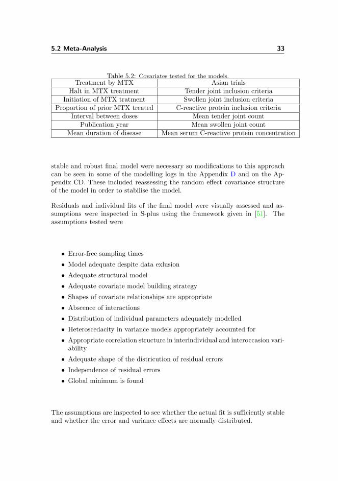
5.2 Meta-Analysis 33
Table 5.2: Covariates tested for the models.Treatment by MTX Asian trials
Halt in MTX treatment Tender joint inclusion criteriaInitiation of MTX tratment Swollen joint inclusion criteria
Proportion of prior MTX treated C-reactive protein inclusion criteriaInterval between doses Mean tender joint count
Publication year Mean swollen joint countMean duration of disease Mean serum C-reactive protein concentration
stable and robust final model were necessary so modifications to this approachcan be seen in some of the modelling logs in the Appendix D and on the Ap-pendix CD. These included reassessing the random effect covariance structureof the model in order to stabilise the model.
Residuals and individual fits of the final model were visually assessed and as-sumptions were inspected in S-plus using the framework given in [51]. Theassumptions tested were
• Error-free sampling times
• Model adequate despite data exlusion
• Adequate structural model
• Adequate covariate model building strategy
• Shapes of covariate relationships are appropriate
• Abscence of interactions
• Distribution of individual parameters adequately modelled
• Heteroscedacity in variance models appropriately accounted for
• Appropriate correlation structure in interindividual and interoccasion vari-ability
• Adequate shape of the districution of residual errors
• Independence of residual errors
• Global minimum is found
The assumptions are inspected to see whether the actual fit is sufficiently stableand whether the error and variance effects are normally distributed.

34 Methods
5.2.1 S-plus
Before starting the modelling process an exploratory data analysis was per-formed in S-plus. This analysis assisted in getting an overview of the data,preliminary inspection for covariates, and to confirm that the data extractionhad been performed correctly.
The following modelling procedure in S-plus was performed using the NLME-function which follows the formulation by Lindstrom and Bates [65]. Efficacydata was excluded from the data set if it came from treatment arms with lessthan 30 patients. This precaution was due to the normal distribution assump-tion for the error of the model. This restriction number was found by lookingat the standard deviation of a binomial distribution, figure 5.1. This excludedone trial from the models with normal distributed error.
Figure 5.1: The standard error of the mean, based on a binomial distribution withp = 0.5
A model was built up by initially making the simplest model possible and re-gressing toward higher complexity until a stable base model was produced. Thisprocedure was necessary because the NLME-function seemed to be highly de-

5.2 Meta-Analysis 35
pendable upon initial parameter estimates. Using the final estimates of theformer model as initial estimate for the new model allowed a progress toward astable base model.A selfStart-function could have been implemented to overcome this problem. Aninitial attempt to estimate initial values by simple calculations in a selfStart-function proved to be inadequate. It was also perceived as futile since the modelspecification, covariates, and random effects were changed from one model runto another and therefore also required constant modification of the selfStart-function.The S-plus modelling was only performed on the ACR20 data and attemptedon the ACR50 data before changing to the NONMEM program. It was per-ceived that the decreased amount of ACR50 data and difficulties constrainingthe parameters caused the instability of the function. The final model log andS-plus script are included on the Appendix CD.
5.2.2 NONMEM
Before shifting to the NONMEM program a comparison of parameter estimatesbetween the two methods were performed. NONMEM has been shown to pro-duce similar results as S-plus [80][102]. Initially the first order conditionalestimate(FOCE)-method was used in the program to find the parameter es-timates. The objective function value was used for the likelihood ratio test.The procedure described above was used subsequently to acquire a model forACR20 and later ACR50. ACR50 was chosen as the principal outcome becauseof its anticipated clinical relevance.A binomial distribution model was also constructed to fit the ACR50 data. Thismodel would take into account the number of patients in the trials as well asallowing the small trials to be included. To stabilise this method the Emaxvalues were logit transformed[16][28]
Emax,i =eβi
1 + eβi(5.5)
where βi is the population parameter value estimated by the model for the treat-ment of the ith trial arm. The estimated parameters were found by minimisa-tion of the likelihood function based on the Laplacian approximation methodof NONMEM[32]. This method did not allow an evaluation of the error modelsince the error was automatically assumed to be binomial distributed and ad-ditive in this model. The residuals were standardised according to Pearson’sresiduals[27]
wresij =nipij − nipijnipij(1− pij)
(5.6)

36 Methods
where pij is the jth proportion of the ith trial arm, ni is the number of patientsin the ith trial arm and pij is the estimated proportion of the model jth datarecord of the ith trial arm.Besides the assumption checks, likelihood profiling was also performed for allparameters. This was accomplished by fixing one parameter to 31 differentvalues in 31 different models and then letting NONMEM estimate the rest ofthe parameters. The objective function values were extracted along with thefixed parameter. A likelihood profile was then created by making a cubic splineapproximation of the data. This permitted to get a better proposition on theconfidence intervals of the model. The significant difference between Emax pa-rameter values of the TNF-α inhibitor treatments by setting two or three treat-ment to the same fixed parameter in an alternative final model.The ACR20 and -70 data was also modelled with both approaches using thesame covariates and random effect structure as the ACR50 model. The finalnormal and binomial distributed models were also simulated using NONMEM.Model parameters were fixed on the final parameter and then 500 simulations ofplacebo and the three anti-TNF-α treatments were made with all covariates setto the standard value or the mean of all the trials. The highest and lowest 2.5% proportion values in the simulations were taken out to make an estimationinterval for the model.The model data was imported into S-plus where it was visualised and handledto check model fits and assumptions. This was performed both simultaneousand after constructing the mathematical models.The final binomial model for the meta-analysis became
yijk =Emax,ij · t
γijijk
Tγij12 ,ij
+ tγijijk
+ εijk (5.7)
Emax,ij =eEMij
1 + eEMij
EMij = β1,ij + b1,j + Iij · β3 +Hij · β4
T 12 ,ij
= β1,ij · eb2,j
b ∈ N (0,Ω), Ω =[b2
1,j 00 b2
2,j
]
εijk = σ ·
√pijk(1− pijk)
nij, σ ∈ N (0, 12)
where tijk and yijk is the time and response proportion, respectively, of thekth sample of the ith trial arm of trial number j, with subscripts of the restof the parameters following this notation. β1,ij is the treatment specific Emaxparameter value, which has 9 levels, one for placebo, one for MTX treatmentonly, 3 for adalimumab dosage levels, 2 for etanercept dosage levels and 2 for

5.3 Pharmacokinetic-Dynamic Modelling 37
infliximab dosage levels.
β2,ij is treatment specific time to achieve half of Emax responders with 2 levels,with or without TNF-α treatment. γij has 3 levels; one for placebo, one for MTXtreatment alone and one for TNF-α inhibitor treatment. β3 is the initiation ofMTX concommitant treatment covariate for Emax, the covariate is multiplied byIij which is one for trials arms initiating MTX and TNF-α inhibitor treatment,and zero for all other trial arms. β4 is the halt of MTX treatment covariatefor Emax, the covariate is multiplied by Hij which is one for trials arms haltingprior MTX treatment.
b21,j and b22,j are the trial level variances for Emax,ij and T 12 ,ij
, respectively. εijkis a binomial distributed variance that depend on the individually predictedproportion of the current sample, pijk = yijk − εijk, and the number of patientsin the trial arm, nij .
As it can be seen, this model will increase toward the level of Emax,ij
5.3 Pharmacokinetic-Dynamic Modelling
The PK-PD modelling was performed on the basis of a simpler literature reviewthan the meta-analysis. Articles containing measurements of TNF-α inhibitorconcentration of the blood were found on the basis of a literature review[74].
All the PK data was extracted using the procedures as in the meta-analysis. Foradalimumab the mean concentrations were extracted from 3 articles[31][69][110].For Infliximab median concentration were extracted from 3 articles[53][68][98],because mean concentrations were only given in one article. For etanercept apublished 2 compartment model, produced from the measurements of 98 patientsreceiving etanercept, was used[114].
Affinities for the three drugs were found in a comparison article[54]. Productionrates, elimination rates, and other parameters were found from mechanisticmodelling and experimtal articles[48][59][64][78].
A six compartment model was constructed in a NONMEM input file. Themodel was supposed to illustrate the impact of the 3 TNF-α inhibitors uponthe concentration of TNF-α. The structure of the model can be seen in Figure5.2.
The model has three different substance concentrations that it illustrates, TNF-α, its inhibitor, and their joint complex. The model contains two volumes,the central volume, the blood in which we measure the concentration, and theperipheral volume.
On the basis of this model it is possible to set up 6 differential equations for the

38 Methods
Figure 5.2: The 6 compartment model
rate of change of the amounts in the 6 compartments over time
dA1
dt= −A1Ka
dA2
dt= A1Ka −
A2
V1(Q+ Cl)− A2A6
V1Kon +
A3
V2Q+
A4
V1Koff
dA3
dt=
A2
V1Q− A3
V2Q
dA4
dt=
A2A6
V1Kon +
A5
V2Q− A4
V1(Koff +Q+ Cl)
dA5
dt= (
A4
V1− A5
V2)Q
dA6
dt= Prod− A6
V1El +
A4
V1Koff −
A2A6
V1Kon (5.8)
where A1−3 is the amount of inhibitor in the absorption, central and peripheralvolume, respectively, A4−5 is the amount in the central and peripheral volumefor the joint TNF-α and inhibitor complex, and A6 is the amount of TNF-α inthe central compartment.Ka is the rate of transfer for the inhibitor drug into the central compartment.V1−2 is the central and peripheral volume, respectively. Q is the transfer rate ofthe TNF-α inhibitor and the complex back and forth between the central andperipheral volume.Cl is the clearance rate for the inhibitor and the complex from the central vol-ume. Kon is the association for TNF-α and its inhibitor to combine into acomplex. Koff is the dissociation rate of the complex.

5.3 Pharmacokinetic-Dynamic Modelling 39
El is the elimination rate of TNF-α. Prod is the production rate of TNF-α,which is set to equal the steady-state elimination without TNF-α inhibitors, i.e.Prod = A6(0)
V1El.
The association and dissociation rates were taken from a publication aboutBiacore experiments[54]. In these experiments the TNF-α inhibitors are immo-bilised on a chip. Soluble TNF-α is then injected at different concentrations.Afterwards the TNF-α is washed of with a buffer. By looking at the rate ofassociation and dissociation of TNF-α at different concentrations, it is possibleto determine their rates.In addition to the changes reflected in the differential equations, TNF-α inhibitoris transferred into the system. Adalimumab and etanercept are administered bySC injection so they are inserted in the first compartment as bolus injections,e.g. a delta function. Infliximab is intravenously infused over 2 hours this meansthat it is included in the model as a constant rate over this time length.This model is based upon a number of physiological assumptions and simplifi-cations:
1. It is possible to perceive this physiological system as compartments witha volume and an amount of substance which only influence each other inthe ways described by the differential equations.
2. All particles in one compartment act as one monolithic amount.3. TNF-α and its inhibitor associate and dissociate at the same rate as in a
Biacore1 set up.4. TNF-α exists only in the central volume, i.e. the blood.5. The production of TNF-α is not influenced by concentrations or such.
This production is the same as the elimination rate of anti-TNF-α naivesystem.
6. The clearance of the combines TNF-α and inhibitor complex is the sameas the clearance of the TNF-α inhibitor.
7. The measurements of inhibitor drug do not include the inhibitor amountin the complex.
8. The transfer rate is the same for the complex as for the inhibitor, and therate is the same back and forth.
Furthermore, the model parameters are estimated using a nonlinear model. Thismeans that we have another layer of assumptions upon this system.Since no PD data was available and the PK data available was sparse, only4 parameters were estimated for adalimumab and infliximab. These were theclearance of the inhibitor, Cl, the transfer constant Q, and the central and
1Biacore is an in-vitro setup to measure the affinity of a drug.

40 Methods
peripheral volume, V1−2. The model was assessed by looking at the model fitalong with the PK-data.After estimating the parameters of the model, the TNF-α concentration weresimulated under the dosing regimes that were seen in the meta-analysis. Foradalimumab three doses were chosen 20, 40, and 80 mg every other week, 10,and 25 mg twice a week for etanercept and 3 and 10 mg/kg at week 0, 2, 6, andthen every 8th week for infliximab.Two outcome measures, maximum and mean, were extracted from the TNF-α concentrations after steady state was achieved at day 88, 41, and 112 foradalimumab, etanercept, and infliximab, respectively. Finally these outcomemeasures were compared with their typical Emax values of ACR20, ACR50 andACR70 from the meta-analysis to see if there is any correlation between theoutcomes of the two analyses.

Chapter 6
Results
The models estimated in this thesis include many aspects about the TNF-αinhibitor treatment. Only a chosen selection of the results are presented in thischapter. In the first section the results of the literature review are displayed. Inthe second section the final model of the meta-analysis along with key figuresare presented. In the final section the results of the PK/PD analysis are shownalong with the comparison between the PD and meta-analysis results.
6.1 Literature Review
The course of action for the literature review can be seen in Figure 6.1. 777publications were found in the three databases. Abstracts from 161 of these werescreened for relevancy ending up with 71 publications. Of these 71 publications,5 were not retrieved either because of language or wrong reference statement.23 of the articles were removed from the search after reading them in full lengthas described below. 17 of those publications were systematic reviews or meta-analyses which did not use any publications not already found in this literaturereview. 5 of the publications were about DBRCTs for TNF-α inhibitor drugswhich are not already marketed and one publication was about a trial whichwere not double-blinded.

42 Results
Figure 6.1: Flow of study selection.

6.1 Literature Review 43
Table 6.1: Summary of included trial arms. Numbers in paranthesis indicate therange of the covariate. Rec.: Recommended. MTX: Methotrexate. Init: Initiated.DMARD: Disease-modifying antirheumatic drug other than MTX. Pub.: Publicationyear. Dur.: Duration. CRP: C-reactive protein. Incl.: Inclusion criteria. ∗: the numerof trial arms on the described subtreatment. †: The median year of first publicationabout the trial arms, paranthesis indicate the range relative to the median. ‡: Themean of the covariate for all trial arms. ?: The median of the inclusion criteria.
Treatment Placebo Adalimumab Etanercept InfliximabTrials - 8 5 7
Trial arms 20 19 9 13High dose∗ - 4 0 7Rec. dose∗ 20 11 7 6Low dose∗ - 4 2 0
Halt MTX∗ 4 10 2 0Cont. MTX∗ 12 7 6 11Init. MTX∗ 4 1 1 2
Halt DMARD∗ 13 19 9 1Cont. DMARD∗ 6 1 0 10Init. DMARD∗ 1 0 0 2
Pub. year† 2004(-5 to +4)2004(-1 to +4)2000(-1 to +4)2004(-5 to +4)Patients‡ 139(12-340) 130(65-318) 161(59-231) 167(12-378)
Disease dur.(mo)‡ 96(9.6-156) 107(8.4-157.2) 92(11-156) 83(9.6-144)Tender joint‡ 28(14-36) 29(19-35) 31(26-35) 27(19-34)Swollen joint‡ 19(8.8-25) 19(12-22) 22(19-25) 18(10-24)Serum CRP‡ 3.3(1.2-6.3) 4.1(1.4-6.6) 3.3(1.7-5.3) 3.0(1.27-4.2)
Incl. tender joint? 9(6-12) 12(9-12) 12(6-12) 6(6-12)Incl. swollen joint? 12(3-10) 10(6-10) 10(6-10) 6(3-10)
Of the final 29 DBRCTs identified, 9 were removed. 4 of those because theyonly included a single dose [18][53][84][110], 2 trials only provided DAS28 asefficacy[33][44], 2 trials did not have publications which adequately describedpatient population[62][82], and one because dose were given per body surface[71],therefore making difficult to compare with the recommended dosing regimen.
As described in Section 5.1, the quality of the studies was not evaluated. If theprotocol of the article described the procedure as double-blinded, randomisedand controlled it was accepted.
The literature review ended up with 8 adalimumab trials, 5 etanercept trials,and 7 infliximab trials which are summarised in Table 6.1. The table includesonly a selection of the patient and protocol descriptions. In Appendix B theindividual arms are listed along with the covariates relevant for the final model.
All the trial arms included various dosages. Adalimumab was given at doses of

44 Results
20, 40 and 80 mg over two weeks, etanercept was given as 20 or 50 mg over oneweek, and infliximab was given at 3, 5, 6, 10, and 20 mg/kg over 8 weeks. Thenormalising of the dosages according to recommended dosage meant that all thedose levels included similar dosages except the high dose infliximab treatementswhich included 4 different dosages.The amount of data points varied from article to article. Some trials onlyincluded the trial end point efficacy given and some included up to 12 datapoints. ACR20 had the most sample points, 360, hereafter ACR50, 323, andlast ACR70, 298.
The etanercept trials did not include any trials above the recommended dosageeven though it has been seen in a trial which was not controlled[49]. No inflixi-mab trial reporting ACR with dosages under the recommended level was foundthough it was seen in one trial[68].
As it can be seen from the table infliximab is the only drug which does notinclude a trial with termination of the MTX treatment. This is because MTX isrecommended as concomitant treatment when treated with infliximab as men-tioned in Section 2.4.1.
In total over 8870 patients were included in the 20 trials in 61 treatment arms.There is 3633, 2057, and 3180 patients allocated at the adalimumab, etanerceptand infliximab trials, respectively.
Table 6.1 also shows that the adalimumab trials include the patients with thelongest RA history in general. It is also seen that adalimumab has the highestnumber of C-reactive protein (CRP). CRP is an inflammatory protein, its con-centration in the blood increases under acute and chronic inflammation. Theetanercept trials also seems to include the patients that suffer of aggressive RAsince they have the highest swollen and tender joint count. The inclusion criteriaseem similar across the trial where only infliximab differs slightly.
6.2 Meta-Analysis
The results in this section primarily focuses on the final model ACR50 with bi-nomial distributed error. The estimates of the model along with their confidenceintervals. The model duplicates for the ACR20 and 70 data are also shown.
In the following sections the binomial model and normal model refer to themodel with binomial distributed error and the model with normal distributederror, respectively.

6.2 Meta-Analysis 45
Figure 6.2: The ACR50 data from all the placebo trial arms of the meta-analysis.
Figure 6.3: The ACR50 data from all the adalimumab trial arms of the meta-analysis.
46 Results
6.2.1 Exploratory Analysis
First part of the meta-analysis was the exploratory data analysis. A selection ofthe the figures used for the exploratory analysis will be shown here. In Figure6.2, 6.3, 6.4 and 6.5 the ACR data of all the trial arms. Comparative figuresfor ACR20 and ACR70 as well as the individual trial arm data by itself can befound in Appendix C.
The time course of all the placebo arms can be seen in Figure 6.2. It canbe seen that all the trial arms do not have the same efficacies. The four trialarms that dissociate themselves from the other on all levels come from ERA[14],PREMIER[20], TEMPO[58] and ASPIRE[97] trials. These trials were all iden-tified as trials initiating MTX treatment in their placebo arms to patients thathave never received it before. The exploratory analysis also revealed that trialswhich required termination of MTX treatment sometimes had a lower propor-tion of ACR responder.
When looking at the figures for all the TNF-α inhibitors, Figure 6.3, 6.4, and6.5, the same MTX tendency could be seen. The effect was most pronouncedwith the ERA[14] and PREMIER[20] where it was possible to compare with atrial arm of the same dose without MTX. It was also possible to see that someof the trials showed increased efficacy proportions when the dose was increased.
This means that the model should test the MTX treatment as a parameterand eventually include it. The figures showing the individual treatment armsefficacies are shown in the Appendix C.
6.2.2 Parameter estimates and confidence limits
The final binomial model included 3 fixed parameters beside the ones mentionedin Section 5.2. These 3 covariates were significant in the likelihood test:
1. Initiation of MTX treatment alone had a different γ than the two othertreatments.
2. The MTX naive patients receiving MTX and TNF-α inhibitor treatmenthad a covariate effect on Emax.
3. The prior MTX patients terminating their MTX treatment also had a co-variate effect on Emax.

6.2 Meta-Analysis 47
Figure 6.4: The ACR50 data from all the etanercept trial arms of the meta-analysis.
Figure 6.5: The ACR50 data from all the infliximab trial arms of the meta-analysis.

48 Results
This means, that the final binomial model found, that the continuation of MTXtreatment or no MTX treatment had the same effect for the patients. Theinitiation of an MTX treatment did stimulate an increased number of respondersboth alone, and with TNF-α inhibitor treatment. The trials including patientswho had not received MTX treatment before was also the trials with RA atits earliest stages. This means that the patients actually had fewer swollen ortender joints at the start of the trial. Terminating the MTX treatment had theopposite effect on the number of responders, which means that removing thistreatment had a negative impact upon suppression of RA.The model assumptions was investigated and the plots can be seen in AppendixE. None of the test led to any serious infringement of the assumptions on whichthe binomial model was based. The estimated parameters of the binomial modelcan be seen in Table 6.2.
In this table it is seen that the patients receiving placebo, meaning no initia-tion of drug treatment, gets the lowest proportion of responders. It is worth tonotice, that the MTX naive patients that receive MTX gets higher proportionalresponses than both adalimumab and infliximab. Etanercept has the highestproportional responders of all the treatments. It is also seen, that the adali-mumab gets a smaller decline in responders than etanercept when set to a lowdose, 6.28% vs. 12.6%, respectively. The increase from a higher dose is largerfor adalimumab than infliximab;7.23% vs. 5.12%. T 1
2was longer for placebo
and MTX treatment than for anti TNF-α.It is noticeable that the effect of MTX treatment on MTX naive patients is notas large for the TNF-α treatment, ranging from 19.3% to 20.7 % because of thelogit transormation as for the placebo treated patients, 30.0 %. At the sametime the cessation of MTX treatment makes a larger negative impact on theanti TNF-α treatments, 12.8% to 14.4%, than on the placebo treated patients,5.54%.The variance components had intertrial variation1 (ITV) of 28.9 and 32.9% forEmax and T 1
2, respectively. The relative standard error2 (RSE) was 50.7 and
39.0 % for Emax and T 12, respectively. As a consequence they have an impact
on the logit transformation and expontial function that they are part.
Likelihood profiling was also performed on all the parameters of the model.This was performed to assess whether the logit transform produced estimatesof standard errors which were erroneous. Four of the likelihood profiles can beseen in figure 6.6 the rest are located on the Appendix CD.On this figure it can be seen that the skewness of the likelihood profiles are notthe same for all the parameters. Notice that the profiles are skewed for both
1ITV= 100 ·√σ2b
2RSE =100*σ2b
SEb. SEb: The standard error of the parameter.

6.2 Meta-Analysis 49
Table 6.2: The parameter estimates of the final binomial model of the ACR50 dataand its lower and upper 95 % boundaries using the standard error provided from NON-MEM. ∗: The parameters are still logit transformed. †: The parameter is exponentiallymultiplied on T 1
2.
Parameter Lower Estimate UpperEmax Placebo (%) 11.1 13.6 16.5Emax MTX treatment (%) 38.4 43.6 49.0Emax Adalimumab (%) 36.6 42.8 49.3Recommended doseEmax Adalimumab (%) 31.0 36.6 42.5Low doseEmax Adalimumab (%) 42.7 50.1 57.5High doseEmax Etanercept (%) 47.2 53.0 58.8Recommended doseEmax Etanercept (%) 34.4 40.4 46.7Low doseEmax Infliximab (%) 34.4 39.2 44.2Recommended doseEmax Infliximab (%) 39.1 44.3 49.7High doseT 1
2Placebo & MTX (Weeks) 7.41 9.30 11.2
T 12
Anti-TNFα (Weeks) 4.96 6.52 8.07γ Placebo 1.29 1.61 1.93γ MTX 1.73 2.10 2.47γ Anti-TNFα 1.09 1.24 1.39Emax covariate for 0.722 0.840 0.958MTX effect on Anti-TNFα∗
Emax covariate for -0.855 -0.586 -0.317termination of MTX treatment∗
Variance of random effects 3.92 ·10−4
8.33 ·10−2 0.166on E∗maxVariance of random effects 2.57 ·10−2
0.108 0.190on T †1
2

50 Results
Figure 6.6: The likelihood profiles for Emax of infliximab at high dose, T 12
of placebo
& MTX, T 12
of anti TNF-α treatment, and γ for placebo. The green and orange
lines are the 95 % boundaries of likelihood profiling and NONMEM’s standard errors,respectively. The red line marks the 3.84 increase of objective function value.
Emax, T 12
and γ parameters. The degree of skewness is different for differentparameters as well as the range of likelihood values. Decreasing the γ param-eter estimate clearly changes the objective function value more than the otherparameters. The 95 % confidence limits according to a likelihood ratio test isalso shown to give another view upon the confidence limits of the parameters.The new boundaries achieved by likelihood profiling is listed in Table 6.3.
It can be seen from Table 6.3 that the estimates differ from those obtainedwith the standard error estimates. Furthermore the boundaries are less than5 % different relatively to the parameter estimation except for the covariates.Normally, a transformation should resolve the likelihood profile skewness. Theeffects with the largest deviations from the NONMEM standard error estimates,are already in a logit tranformation out of neccessity, and therefore anothertransformation seems unreasonable.The confidence limit of the binomial model was also assessed by simulating the

6.2 Meta-Analysis 51
Table 6.3: The lower and upper 95 % boundaries of the likelihood profiling. Thenumber in paranthesis is the difference to the standard error boundaries relatively to
the parameter estimate,Intβ,LL−Intβ,SE
β, where Intβ,LL and Intβ,SE is the confidence
interval of the profiles and NONMEM’s standard error respectively. Negative valuesmeaning being NONMEM’s estimate is the lowest and vice versa . ∗: The parametersare still logit transformed. †: The parameter is exponentially multiplied on T 1
2.
Parameter Lower UpperEmax Placebo (%) 11.1(-0.252) 16.5(0.124)Emax MTX treatment (%) 37.9(-1.24) 49.9(1.98)Emax Adalimumab (%) 37.3(2.01) 48.6(-1.85)Recommended doseEmax Adalimumab (%) 30.7(-0.754) 43.0(1.04)Low doseEmax Adalimumab (%) 43.5(1.74) 57.0(-1.22)High doseEmax Etanercept (%) 46.3(-1.39) 60.2(2.30)Recommended doseEmax Etanercept (%) 34.0(-0.639) 47.5(1.36)Low doseEmax Infliximab (%) 33.6(-1.87) 45.3(2.57)Recommended doseEmax Infliximab (%) 38.3(-1.43) 51.4(3.01)High doseT 1
2Placebo & MTX (Weeks) 7.14(-1.69) 12.2(1.00)
T 12
Anti-TNFα (Weeks) 4.88(1.28) 8.94(1.07)γ Placebo 1.29(3.70) 2.01(4.81)γ MTX 1.77(1.69) 2.48(0.529)γ Anti-TNFα 1.11(2.24) 1.38(-1.08)Emax covariate for 0.686(-3.98) 1.01(6.41)MTX effect on Anti-TNFα∗
Emax covariate for -0.971(-19.6) -0.184(22.4)termination of MTX treatment∗
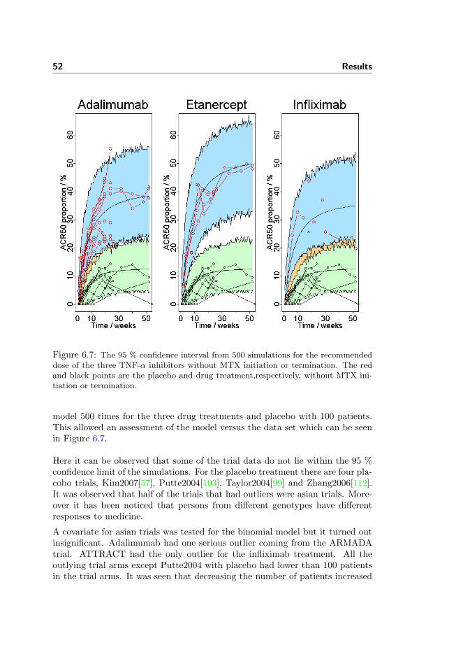
52 Results
Figure 6.7: The 95 % confidence interval from 500 simulations for the recommendeddose of the three TNF-α inhibitors without MTX initiation or termination. The redand black points are the placebo and drug treatment,respectively, without MTX ini-tiation or termination.
model 500 times for the three drug treatments and placebo with 100 patients.This allowed an assessment of the model versus the data set which can be seenin Figure 6.7.
Here it can be observed that some of the trial data do not lie within the 95 %confidence limit of the simulations. For the placebo treatment there are four pla-cobo trials, Kim2007[57], Putte2004[103], Taylor2004[99] and Zhang2006[112].It was observed that half of the trials that had outliers were asian trials. More-over it has been noticed that persons from different genotypes have differentresponses to medicine.
A covariate for asian trials was tested for the binomial model but it turned outinsignificant. Adalimumab had one serious outlier coming from the ARMADAtrial. ATTRACT had the only outlier for the infliximab treatment. All theoutlying trial arms except Putte2004 with placebo had lower than 100 patientsin the trial arms. It was seen that decreasing the number of patients increased

6.2 Meta-Analysis 53
Table 6.4: The increase of objective function values (OFV), respective likelihoodratio tests significance, and new parameter estimates when setting two or three rec-ommended doses at the same parameter.
Combination ∆OFV Significance Parameter estimate (%)Adalimumab + 13.0 3.04·10−2 43.8EtanerceptAdalimumab + 1.77 18.3 43.4InfliximabEtanercept + 17.7 2.59·10−5 44.8InfliximabAdalimumab +
19.8 4.84·10−5 43.3Etanercept +Infliximab
the range of the simulation confidence intervals. This could partly explain theoutlying tendency for these trial arms.
6.2.3 Significant Difference of Treatment
It was neccessary to derive whether the treatments were significantly differentor not. The likelihood profiles and standard errors could be used to give anestimate which is seen on the Appendix CD. But a more proper approach wasto constrain two or three anti TNF-α treatments of recommended dose to thesame fixed effect. The models returned with the increases in objective functionvalue as seen in Table 6.4.
In the table it can be seen that Adalimumab and Inliximab are the only drugswhich are not significantly different according to the meta-analysis.
It can also be seen that the combination of adalimumab and infliximab oddlyenough increases the common parameter to higher levels than both of the drugsformer estimates. The likelihood ratio test results of the combination of alldrugs compared with combination of Etanercept and Infliximab should also benoted. It is larger because the model is reduced by 2 parameters compared withone, which means that the likelihood ratio test must be taken with 2 degrees offreedom.

54 Results
6.2.4 Typical Values and Time Courses
The final binomial model was also used to make parameter estimation on theACR20 and ACR70 data which are listed in Table 6.5 and Table 6.6.
The model assumptions analysis for the ACR20 model of Table 6.5 can be foundon the Appendix CD. The model assumptions are not met with the same degreeof adequacy as for the ACR50 model, seen on the appendix CD. The parameterestimates fits the data sufficiently, considering that the model has been fittedto another data set.
Looking at Table 6.5, it is noted that the Emax estimates has increased. Thisindicates that a higher proportion of patients receive the lower level response. Itcan also be seen that T 1
2has decreased, which shows that half of the responders
sooner achieves the ACR20 response than the ACR50 response. This makessense since it is impossible to achieve an ACR50 response without achieving aprior ACR20 response.
It can be seen that placebo and MTX treatment have approximately the sameparameter estimate. At the same time, γ for TNF-α treatment is close to one.Both of the covariates have approached 0 compared to the results of the ACR50model. Both of the variances have increased, and the 95 % boundaries nowinclude 0, and have an ITV of 31.5 and 48.9 % for Emax and T 1
2, respectively,
and a RSE of 53.3 and 60.7 % for Emax and T 12, respectively. Meaning that
the variance components have increased and they have becomed more uncertainrelatively to the ACR50 model.
The model assumptions analysis for the ACR70 model of Table 6.5 can be seenon the Appendix CD. The ACR70 model proved to be far inferior to satisfy thenormal distribution assumptions. As mentioned in Section 6.1, the ACR70 dataset was sparser than the two other data sets, which could cause some of theproblems.
Looking at Table 6.6, it can be noted that the Emax estimates has fallen con-siderably. This indicates that a lower proportion of patients receive this levelresponse. It can also be seen that T 1
2has increased compared to the ACR20
and ACR50 models, in Table 6.5 and 6.2, which shows that the patients achievethis level of response later.
The γ parameters have increased for all treatments, indicating that there is aslower increase in the model function. The covariate on Emax for methrotrexate(MTX) treatment initiation has increased to the highest value of all the threebinomial models. At the same time, the covariate on Emax for MTX treatmenttermination has increased slightly toward zero, which indicates a reduced effecton ACR70 of MTX termination.
Compared to the ACR20 and ACR50 the random effects have decreased and
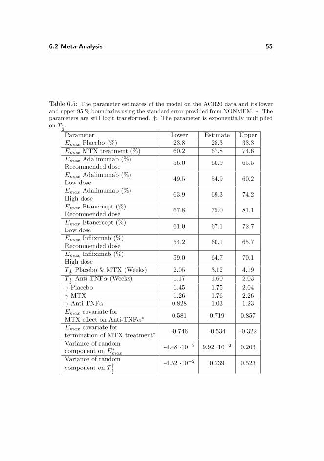
6.2 Meta-Analysis 55
Table 6.5: The parameter estimates of the model on the ACR20 data and its lowerand upper 95 % boundaries using the standard error provided from NONMEM. ∗: Theparameters are still logit transformed. †: The parameter is exponentially multipliedon T 1
2.
Parameter Lower Estimate UpperEmax Placebo (%) 23.8 28.3 33.3Emax MTX treatment (%) 60.2 67.8 74.6Emax Adalimumab (%) 56.0 60.9 65.5Recommended doseEmax Adalimumab (%) 49.5 54.9 60.2Low doseEmax Adalimumab (%) 63.9 69.3 74.2High doseEmax Etanercept (%) 67.8 75.0 81.1Recommended doseEmax Etanercept (%) 61.0 67.1 72.7Low doseEmax Infliximab (%) 54.2 60.1 65.7Recommended doseEmax Infliximab (%) 59.0 64.7 70.1High doseT 1
2Placebo & MTX (Weeks) 2.05 3.12 4.19
T 12
Anti-TNFα (Weeks) 1.17 1.60 2.03γ Placebo 1.45 1.75 2.04γ MTX 1.26 1.76 2.26γ Anti-TNFα 0.828 1.03 1.23Emax covariate for 0.581 0.719 0.857MTX effect on Anti-TNFα∗
Emax covariate for -0.746 -0.534 -0.322termination of MTX treatment∗
Variance of random -4.48 ·10−3 9.92 ·10−2 0.203component on E∗maxVariance of random -4.52 ·10−2 0.239 0.523component on T †1
2

56 Results
Table 6.6: The parameter estimates of the model on the ACR70 data and its lowerand upper 95 % boundaries using the standard error provided from NONMEM. ∗: Theparameters are still logit transformed. †: The parameter is exponentially multipliedon T 1
2.
Parameter Lower Estimate UpperEmax Placebo (%) 4.35 5.90 7.94Emax MTX treatment (%) 18.8 22.8 27.3Emax Adalimumab (%) 21.0 26.5 32.8Recommended doseEmax Adalimumab (%) 14.2 19.5 26.1Low doseEmax Adalimumab (%) 24.3 32.4 41.6High doseEmax Etanercept (%) 25.1 31.3 38.4Recommended doseEmax Etanercept (%) 16.6 20.8 25.7Low doseEmax Infliximab (%) 16.5 20.9 26.2Recommended doseEmax Infliximab (%) 18.9 25.4 33.1High doseT 1
2Placebo & MTX (Weeks) 10.6 15.4 20.2
T 12
Anti-TNFα (Weeks) 10.9 15.0 19.1γ Placebo 0.693 1.62 2.55γ MTX 2.35 3.10 3.84γ Anti-TNFα 1.13 1.34 1.55Emax covariate for 0.940 1.03 1.12MTX effect on Anti-TNFα∗
Emax covariate for -0.599 -0.399 -0.199termination of MTX treatment∗
Variance of random effects -0.107 7.81 ·10−2 0.263on E∗maxVariance of random effects 7.28 ·10−2 4.23 ·10−2 0.157on T †1
2

6.2 Meta-Analysis 57
Table 6.7: The final proportion ACR20 responders which have an ACR50 responseand the proportion of ACR50 responders having an ACR70 response according to theparameters of the binomial models.
Treatment ACR20→ 50 (%) ACR50 → 70(%)Placebo 48.0 43.4MTX treatment 64.4 52.2Adalimumab Recommended dose 70.4 61.9Adalimumab Low dose 66.6 53.2Adalimumab High dose 72.3 64.6Etanercept Recommended dose 70.7 59.1Etanercept Low dose 60.2 51.3Infliximab Recommended dose 65.2 53.4Infliximab High dose 68.4 57.2
they are not significant, according to the 95% confidence interval. The randomeffects have ITV of 27.9 and 20.6 % for Emax and T 1
2, respectively. The RSE for
the random effects of 121 and 139 % for Emax and T 12, respectively, displays the
uncertainty of the estimate. This means that the random effects aConsideringthe Emax estimates for all three response levels, it is possible to estimate theproportion of responders which are having the next level response. These resultsare given in Table 6.7.
In Table 6.7 it can be seen, that according to this analysis, placebo has thelowest proportion of patients achieving higher ACR responses. It can also beseen that adalimumab at high dose is the drug which gets most of its respondersto achieve the higher levels of response. Infliximab is the TNF-α treatment atall levels of dosage with the lowest score proportion of responders achieving thenext level.
In Figure 6.8 the typical efficacy time courses for patients at the 3 anti TNF-αtreatments and placebo for both the binomial and normal model are presented.It is seen that the etanercept treatment always scores the high proportion of re-sponders. Adalimumab and infliximab have comparable responses at the ACR20level but the difference between the two treatments increases when the responselevel increases.
It is not possible to compare parameter values between the two types of mod-els, because they do not use the same parameters and covariates. The normalmodel includes a tolerance part. This makes the other parameters increase asa response leading to a faster increase, which deludes as the model approachesone year. This results in lower efficacy proportions compared to the binomialmodel. It is also seen that there is a larger difference between the two antibodiesand etanercept than in the binomial ACR50 model.

58 Results
Figure 6.8: The typical efficacy time courses for the three anti TNF-α treatmentsand placebo according to the binomial model at ACR20(top left), 50(top right)and 70 (lower left). The typical time course for ACR50 according to normalmodel(lower left).
The difference between the two models does not lie in the typical time coursesas well as in the covariates included in the final model. The binomial model in-cludes a γ parameter for MTX treatment and a Emax covariate for terminationof MTX treatment. Here the binomial model includes a tolerance function anda covariate for Emax which depends on the mean number of tender joints andmean serum C-reactive protein in serum for the patients in the trial arm.
6.3 Pharmacokinetic-Dynamic Modelling
The analysis results presented in this section concerns the PK-PD model. InFigure 6.9 and 6.10 the PK-data is shown.

6.3 Pharmacokinetic-Dynamic Modelling 59
Figure 6.9: The PK-data for adalimumab. Single dose(left) and multidose (right)mean data from 3 trials[69][31][110] with 13 different trial arms. The trials are namedin the key according to the acronym of the trial or the first author of the publication.
In the part of Figure 6.9 the adalimab mean sample values are seen. The dosagein the two single dose adalimumab trials were given as a dosage per kilo ofweight and as a single bolus injection. For these single dose trials it is seenthat the serum concentration quickly declines in the first short time span andhereafter declines at a slower rate.
The CHANGE trial was with asian patients receiving a SC dose every secondweek. The samples were taken prior to administration of the drug at week 2, 4,and then every 4th. The serum concentration stabilised after week 8.
The serum concentration samples from the bolus trials with the same dosagewere comparable. The serum concentration of the Weisman trial at 1 mg/kgafter 2 weeks were almost identical to the serum concentration of the CHANGEtrial at 80 mg. The same tendency were seen for the 0.5 mg/kg dose of Broeder,Weisman and 40 mg dose of the CHANGE trial. This reflects that the meanweight of the patients in the single dose trials was about 70 kg.
In Figure 6.10 the infliximab median sample values are seen. The single dosesamples of the Kavanaugh trial did have an initial fast decline. All the trialarms had median sample concentrations over 0.1 µg/mL until the end of thetrial at week 12. The concentrations of the 5 and 10 mg/kg treatment armbecame similar after week 8.
The ATTRACT and the Maini trial were sampled right before and 1 hour afterthe two hour IV injection given at day 0, 14, 42, and then every 4th or 8th week.The Maini trial had last dosage at week 16 where the ATTRACT trial continuedfor a year. It can be seen that the same dosage and interval across different trialsproduce the same median serum concentration. It can also be seen that thesame dosage with longer time intervals between drug administration produced

60 Results
Figure 6.10: The PK-data for infliximab. Single dose(left) and multidose (right)median data from 3 trials[98][53][68] with 10 different trial arms. The trials are namedin the key according to the acronym of the trial or the first author of the publication.
comparable median serum concentrations 1 hour after the end of infusion butlower prior to the infusion.
The limit of quantification of the samples from the Maini trial was 0.1 µg/mL.This level was reached for many of the median sample concentrations of the 1mg/kg arm after week 4. For the two other treatment arms of this trial thislevel was first reached after termination of treatment. The level was reached atweek 22 and 26 for respectively the 3 and 10 mg/kg trial arms. This suggestthat infliximab is cleared from the blood in most of the patients when receivingsmall doses of the drug.
6.3.1 Pharmacokinetic Modelling
The parameters were estimated by NOMEM using the procedure described inSection 5.3. The model was checked by looking at the model fit to the data.The estimated parameters are given in Table 6.8 along with the fixed parametersand the parameters of the etanercept model.
Table 6.8: The estimated values for adalimumab and infliximab as well as the valuesfrom the etanercept model[114] and the biacore affinities[54]. ∗: The parameters fromthe etanercept model[114]. †: The BIAcore affinities[54].
Drug V1 [L] V2 [L] Cl [mL/h] Q [mL/h] Kon [M−1h−1] Koff [h−1]Adalimumab 2.42 1.05 12.2 0.226 6.08·10−9† 0.170†
Etanercept 5.97∗ 2.05∗ 72.0 ∗ 0.065∗ 20.3·10−9† 0.240†
Infliximab 2.54 3.26 12.8 0.181 8.64·10−9† 0.236†

6.3 Pharmacokinetic-Dynamic Modelling 61
As it can be seen these three drugs does not produce similar parameters. Ada-limumab has the smallest volumes by far and etanercept has the largest. Thismeans that etanercept apparently is distributed over a far greater volume thanthe two other drugs. This could be due to the fact that etanercept is a receptorwhere the two other drugs are antibodies. Interpretation problems can arisewhen looking at the volumes of a PK-PD analysis. The difference of the centralvolume between drugs does not mean that the patients treated with the dif-ferent drugs have different volumes of blood. Instead, the drugs have differentmechanisms of dispersion.
The clearance of the two antibodies, adalimumab and infliximab, are very closewheras the clearance of etanercept is about 6 times as big. The high parametervalue denotes, that etanercept is cleared from the body far quicker than the twoother drugs which explains the shorter time interval between administration ofthe drug.
The rate of transfer is also comparable for the two antibodies, whereas it issmaller for etanercept. This could be interconnected with the fact that etaner-cept has a far larger central volume.
When looking at the association rate it is quickly seen that etanercept has thebest ability for TNF-α association. At the same time, it is also the quickestto dissociate from the cytokine closely followed by infliximab. Looking at theassociation/disassociation ratio, etanercept has the best score with infliximabin second followed closely by adalimumab. This indicates that etanercept doesnot require the same concentration to bind the same amount of TNF-α.
The two SC drugs also had bioavailability parameters of 64.0%[10] and 62.6%[114]for adalimumab and etanercept, respectively. This is the amount of the drugwhich comes into the circulation after being injected into the body by SC route.
Beyond these parameters, two common parameters were also used. These wereretrieved from the litterature.
• The first order absorption rate constant, KA, set to 0.03 h−1[64].
• The elimination of TNF-α, set to 0.036 h−1[48].
• The concentration of TNF-α, set to 50 pg/mL[59].
• The molecular weight of TNF-α, set to 17 kDa[78].
The first order absorption rate constant is only neccessary for adalimumab andetanercept since infliximab is introduced directly into the blood by IV infusion.

62 Results
6.3.2 Pharmacodynamic simulation
Using all the parameters shown, drug and TNF-α time profiles were simulateddifferent doses with the three different drugs.
• Adlimumab given in doses of 20, 40 and 80 mg every other week.
• Etanercept given in doses of 10 and 25 mg twice a week.
• Infliximab given in doses of 3 mg/kg and 10 mg/kg at week 0,2, 6 andthen every 8th week.
These doses were chosen to respresent the recommended, low and high doses ofthe trials in the meta-analysis. The results of the simulations can be found inFigure 6.11.
Figure 6.11: The PKPD simulations of the three TNF-α inhibitors at differentlevels of dosage. The proportion of free TNF-α is relative to the concentrationbefore introduction of the TNF-α inhibitor. High, Rec., and low in the key labelrefers to respective high, recommended and low dose.

6.3 Pharmacokinetic-Dynamic Modelling 63
It also displayed in the figure, that the three drugs appear in very differentconcentrations. Infliximab has by far the highest concentration. This is partlydue to the fact that it is the only IV drug. Even though the infusion is dis-tributed over two hours, it it still a lot faster than the absorption from the SCadministration. At the same time infliximab is given in doses of 3 and 10 mg/kgcorresponding to about 210 and 700 mg given to a patient over 2 hours. Foradalimumab and etanercept between 20 and 80 mg are given per SC infusion.It is seen that adalimumab and etanercept reaches a steady-state profile at ap-proximately 40 and 20 days, respectively. In contrast, infliximab is given with avaried interval until week 6 and therefore the concentration profile changes overtime.Looking at the concentration of TNF-α a large difference between the drugscan be observed. These are both related to the the concentrations of the drugsbut also to their affinities. The drugs keep the TNF-α concentrations below 2percent of the former level. The TNF-α curves seem to display inverse profilesof their respective drug concentration profiles.Adalimumab has the largest variation in the TNF-α concentration comparedto the relatively small variation in drug concentration. Etanercept, at recom-mended dose, keeps the cytokine concentration relatively low compared to itsown concentration. Infliximab manages to keep the TNF-α concentration reallylow after treatment but the effect diminishes as time between dosage increasesand the concentration of the drug gets below 10 mg/L.To compare the simulated TNF-α concentrations with the results of the meta-analysis, outcome measure were extracted after a steady state was achieved. InFigure 6.12 the Emax estimates for ACR50 of all the TNF-α treatments andplacebo have also been shown against their respective mean and maximum pro-portion free TNF-α concentrations. In the figure Emax estimates for ACR50have been shown against the mean of the drug concentration.
In the figure it can be seen that the relationship between then mean concentra-tion of TNF-α and the Emax estimates is not definitely semilogarithmic. Thisis mainly due to the relatively high mean value for the free concentration ofTNF-α that infliximab at high dosage produce compared to the Emax estimate.
A more distinct semilogarithmic relationship between the Emax estimates forACR50 and the TNF-α concentrations is observed from the upper right of Figure6.12. It can be seen that the treatment with the highest amount of respondersalso is the one with the lowest value of maximal proportion of free TNF-α andvice versa.In the lower left part of Figure 6.12 the drug concentration of the different drugdosages has been visualised again their respective Emax parameter estimates.There is no systematic tendency between the two measures except when lookingat one drug by itself. This reinforces the hypothesis that the drug concentration

64 Results
Figure 6.12: The Emax estimates for ACR50 of the binomial model against theirrespective mean (upper left) and maximum(upper right) proportion of free TNF-αafter steady state. A logarithmic least square tendency line has been inserted in bothof these subfigure. The Emax estimates for ACR50 against their respective mean drugconcentration (lower left.
is not crucial it is rather a relationship between the concentration and pharma-codynamic characteristics of the drug that is important.The same figures were produced for the ACR20 and ACR70 model, which canbe seen in the Appendix F, these figures showed the same tendency.

Chapter 7
Discussion
In this chapter the methods and results of this thesis will be discussed. Thechapter is retrospective on alternatives of the decisions taken in this thesis aswell as a view on future work and hypotheses with the current results. In thefirst section the literature review is discussed. Thereafter the meta-analysis aswell as the implications of the results will be analysed. In the last section, adiscussion of the PK-PD analysis is presented.
7.1 Literature review
The data on which the meta-analysis is built must be discussed first hand. Themeta-analysis was performed according to the rules of literature review. A newsearch might provide additional trials but this is unlikely. The drugs have al-ready been approved in most industrialised countries and the newest publicationincluded in the meta-analysis came from a comparitor drug trial with a new bi-ological DMARD.
Trials were found in the literature search, but not used. Among these were thesingle-dose trials. These included additional efficacy proportions within the timeinterval after the first dosage. Inclusion of these trials could have made a morereliable model for the first interval between first and second dosage. But the

66 Discussion
trials were excluded because the trial setup were unlike the clinical situation. Inthis situation the patient knows that he or she is going to have multiple dosagesand therefore the psychological situation does not resemble that of the singledose trial. It is not known whether the single dose trials have an increased ordecreased proportion of responders compared to the multidose trials.Two DBRCT trials were excluded from the meta-analysis based on a lack ofbaseline characteristics. The two trials were excluded because they did notinclude baseline characteristics about disease duration or proportion of femalepatients in the trial arms. These two baseline characteristics were some of thecharacteristics required to include a trial in the meta-analysis. Both trials wererelatively small, both under 60 patients in the trial, so it is believed that theywould not have changed the model decisively. This is supported by the assump-tion checks where exclusion of the small trials did not have critical influenceon the parameter estimates. But an additional model should be built includingthese two trials to ascertain their importance.The model could also be improved if it were supported by additional data. Inmany of the articles, the protocol indicated that ACR responses were measuredseveral times during the trial, but still only trial endpoints were given. In otherarticles, the number of ACR20 responders were given at many time points butfewer samples were given for the other levels. An email was send by supervisorHenning Bliddal to the Danish departments of the pharmaceutical companiesdistributing the relevant drugs, requesting published and unpublished data fromall DBRCTs. This was done both to ascertain that the current data was cor-rect and provide additional data. The email named the found trials and alsorequested data from any trials not publicated. No reply was ever received onthe enquiries.A major support for an analysis like this would be publication of trial databasesafter an approval of the drug by the regulatory agencies. In consideration tothe workburden of this and to the publication rights of clinical collaborators,the drug companies should have a given time interval before releasing the data.This would have several beneficial societal effects upon several levels.
• Meta-analyses could be performed with data on individual patient levelwithin trials.
- The covariates of the individual patient could be used instead of themean of all the patients in the trial arm. This would make morereliable models which accounted for the covariates on an individual.When using mean values of an trial arm in a meta-analysis like thisone, it is never known whether the responders generally have valuesbelow or above the mean value. It would be possible to find baselinecharacteristics which were significant for the response of a patient.
- It would be possible to analyse the trial to trial variation in relation

7.1 Literature review 67
to prior treatments and the geographical origin of the trial. If thesecharacteristics were properly accounted for in the model the real trialto trial variation could be estimated.
- All data would be public so the meta-analyses would not be restrictedonly to end-points of the trials. The current situation where the dataavailable is dependent upon authors and publicists is not durable.
• The statistical methods of the pharmacological industry could be inves-tigated. The public would have an additional possibility to assess thestatistical results of the trials in addition to the national regulatory agen-cies.
• The data could be used for educational purposes at universities. Thestudents would learn how large data sets are managed in the industry andapply the methods they have learned on real patient or PK-PD data.
• New trials of drugs could be designed to inquire the same characteristics.This means that covariates could be investigated more broadly for meta-analyses.
• A safety meta-analysis could be performed if the data included the timepoint of adverse events at individual level were provided. It has not beenfeasible in this meta-analysis to use the safety data of the trials because oftheir different time lengths. The number of patients having adverse eventscould be processed like the number of ACR responders has been in thisthesis.
• Publication bias could be avoided. Trials which are unsuccessful in someway are sometimes not publicated creating a publication bias in the meta-analyses. If drug companies were forced to deliver all trial data this couldbe avoided.
Several criteria should be set for the format of the databases. The units to usefor different data categories and the file format should be clearly specified. Itshould also be decided whether the data should be handled by the companiesthemselves or by a division under the regulatory agencies.The companies could also benefit from this proposal since it would be easier toassess competitor drugs and stop the development of drugs showing inadquateoutcomes.A concern about this proposal could be the possible abuse of the data deliv-ered. Unfit mathematical methods could be used purposely or unpurposely tomispresent the data of certain drugs and publicate these results. But the samesituation exists today. The reviewers of the scientific journals are already as-sessing the methods used for current meta-analyses. Providing the analysistswith additional data should only increase the chance of producing mathematicalmodels which represents drugs of the trials adequately.

68 Discussion
Since the model is confined by the amount and quality of data, the subject hasbecome relevant to the thesis. Therefore the proposal was developed by theauthor as a solution to some of the problems of the final model. This would bea political decision outside the scope of this thesis, which is mentioned due toits many beneficial societal effects.
7.2 Meta-analysis
The meta-analysis was built upon a nonlinear mixed-effects modelling approach.The estimation of these mathematical models are complex and several approx-imations are neccessary to use the mathematical models. An easier approach isthe linear mixed-effects model where an iterative technique is not necessary inorder to estimate the parameters.A linear model based on polynomiums of higher order could be constructed.Such a model can mimic the behavior of most data, but the parameters esti-mated are hard to interpret into behaviors of the different patient treatments.This and other advantages mentioned in Section 3.2 contributed to the decisionof using nonlinear mixed-effects modelling in the meta-analysis. Future work ona meta-analysis like this could include a comparison between linear and nonlin-ear models.Another model function than the sigmoid Emax could also have been used. Anexponential function or an biexponential model could be used instead since thesefunctions also are able to mimic the behaviour seen in the data. These functionswere initially considered but in lack of a robust method to assess the optimalfunction, the Emax function was chosen. Further work with meta-analyses ofthese drugs in RA should include a comparison between model functions.The procedure of the model development was performed in an iterative ap-proach. The S-plus program was changed when found inadequately robust forparameter estimation. In retrospect, several techniques could increase the ro-bustness of the model.
• Parameters could have been transformed in order to limit their range.
• Correlation and the number of the random effects could have been reduced.
• Certain fixed parameters could have been removed to decrease complexityof the function.
The same procedures used in S-plus could also have been used in the R pro-gram. Here it would have been possible to implement the binomial model byusing the glmmML package[21]. This package includes functions that allow

7.2 Meta-analysis 69
the user to use a model with binomial distributed errors as well as use theGauss-Hermite quadrature for parameter estimation. Additional modelling ef-forts should include a comparison with the implementation of this numericalintegration method.In the end, the ACR50 was chosen as the primary objective of the model. Thisproduced a model which fitted excellent to the clinical important criteria butpoorer on the other responses. Another approach could have been to fit themodel to the entire data set at one time. In this way the model structure wouldbe chosen on the basis of all the ACR data. Covariates would not be includedunless they were significant on all the data. In a comprehensive analysis, thisapproach should also be investigated and compared to the model fitted to oneresponse level.An entirely different approach to the problem would be to model efficacy of theTNF-α treatments relative to their control arm, the risk difference,(p− q)1, or
odds ratio,(
( p1−p )
( q1−q )
)1. This would yield numbers that were a direct expression
of the treatment effect. These two measures were visualised for the data in theexploratory analysis, but no evident model function for the data was found.There is also a problem by using the odds ratio because it assumes that youhave a number of responder for both control and treatment arm. If the controlarm has 0 responders it renders an odds ratio of infinite no matter whether thetreatment arm has 1 or 200 responders out of 200 patients.The risk difference can be used as the data to be fit. But it changes the error ofthe model. The variance for risk difference is the sum of the variance of both,and 2 times the covariance of the probability of both the trial if they are notindependent[81].An easy approach would be to use the given proportions of the samples as theirprobabilities.Another approach would be to initially build a model for the ACR scores. Theprediction probabilities of this model for the samples could then be used tobuild the risk difference model. Both approaches assume that the variance oftrial arms are binomial distributed and independent. This is a reasonable as-sumption given that the patients are randomly allocated to the trial arms. Thiscould be performed in NONMEM by using a normal distributed model with thevariance of the error fixed to one. This error should then be multiplied by√
p(1− p)N
+q(1− q)M
(7.1)
where p and q is the estimated probability for the given sample for placebo andtreatment arm, respectively, N and M are the number of patients in the placeboand treatment arm, respectively. This approach would produce a correct risk
1p and q being the response proportion of control and TNF-α treatment, respectivley.

70 Discussion
difference model with respect to the error as long as the two trials have inde-pendent variance of errors.
In this thesis it was assumed that the trial to trial variation could be adequatelymodelled by introducing random effects on the Emax and T 1
2on trial level. The
random effects should model a tendency for the trial on the parameters. In thisway the trials could vary and typical value could still be found for the para-meters. To facilitate the introduction of these random effects they were eitherincluded in an expontial function or in a logit tranformation. This was done toavoid having negative or 0 typical values for Emax and T 1
2.
This has the implication that the impact of the variance components was de-pendent upon the typical value influenced. For the exponential function it isalso given that
1− e−x < ex − 1, x 6= 0 (7.2)
meaning that the exponential function makes a larger absolute impact on thefinal value when the random effect is positive than when it is negative. Theconsequence is that the typical value will be estimated lower than if the expo-nential function was not used. Another feature of the exponential function isthat its absolute value impact increases when the typical value increases. Thisrequires that the trials of different TNF-α treatment should have approximatelythe same distribution of random effects. If the trials of one TNF-α treatmentincludes more positive random effect values than the two other treatments, itstypical values will be underestimated and vice versa if it includes more negativerandom effect. This signifies the importance of inspecting the distribution ofthe random effects both with respect to treatments but also with respect tocovariates included.
The random effects included in the logit transformation has another impact.Its impact has an even distribution around 0.5 when the estimated parameterequals 0. The distribution becomes skewed toward 0.5 when the estimated valuemoves away from 0. The range of the distribution also decreases when the ty-pical value moves away from 0.5.
The exponential function and the logit transformation were both necessary stepsin order to make the model work, and the modelling tasks could not have beenperformed without them. They facilitate reliable estimates for the differenttreatments as long as the random effects are identical distributed across trialsof different drugs.
There is another approach which could solve the dependence of variance com-ponent tranformation. This is to use the NONMEM procedures produced fordata including a level of quantification. In PK-PD analysis it occurs, that thedata provided include a level quantification. This is due to the inaccuracy ofthe sample methods when samples have concentrations below a certain level.This causes all sample values below that level to be set at the same value. Thisof course has implications on the distribution of samples, thereby a correction

7.3 Pharmacokinetic-Dynamic modelling 71
of the distribution of errors and random effects are necessary. Procedures havebeen evolved in NONMEM which compensate for the distribution of the dataallowing the analysists to make a more correct model. Transforming these pro-cedures into the framework of this meta-analysis could facilitate independenceof exponential functions and logit transformations for the random effects.
The results, indicating that etanercept is significantly better, could also be ar-gued to be a result of publication bias. The drug with the least trials identifiedalso became the most efficacious. It could be argued that the same number ofcompleted trials are necessary in order to get a drug approved for clinical prac-tice. This raises the question whether all trials with etanercept have resultedin publications. If they have not been published, the argument for withholdingthis information from the public must be revealed.
The sensitivity of this binomial model is part of the future work that ought tobe conducted to substantiate the results of this analysis. A simple sensitivityanalysis could be the construction of a simple model. This model could be usedon a data set consisting of one data point for each trial arm for 6 months. Thedata could be in the risk difference or odds ratio in order to assess whether themodel has adequately accounted for the inter trial variation. Comparing theseresults with the results of the final binomial model could support the claims ofthe meta-analysis.
7.3 Pharmacokinetic-Dynamic modelling
The general PK-PD model was built on several physiological and biochemicalassumptions and simplifications mentioned in Section 5.3. The model is very de-pendent upon them and they are the same for every drug. This PK-PD modelwas built to make inferences about the relation between the TNF-α concen-trations and the Emax parameters of the drugs. Since the physiological andbiochemical assumptions are the same for every drug they should not pose aproblem to the ambition of the PK-PD model.
After inspecting the data, it was chosen to include a peripheral compartmentfor the TNF-α inhibitor. There was a steeper fall in the concentration rightafter the bolus injections and the 2 hour IV infusion of adalimumab and infli-ximab than later. As a consequence a peripheral compartment for the complexof TNF-α and its inhibitor was included, since the inhibitor component of thecomplex is the greatest part of the mass. It could be argued that there was noreason to include it for etanercept for which no bolus or IV infusion data wasfound. The etanercept model adapted from the article[114] included a peripheralcompartment. Therefore it was infered that the assumption was appropriate.
The estimation of PK parameters for the two antibodies produced outcomes

72 Discussion
which were comparable. The same approach and model were used for bothadalimumab and infliximab. There is a difference between using mean concen-tration for adalimumab and using median concentrations for infliximab. It wasassumed that this effect was minor after studying the samples means and medi-ans of the ATTRACT trial[98], which displays both of the measures. The meanconcentrations were always higher than the median concentration with approx-imately the same amount at every time point, approximately 2-5 µg\mL. It isassumed that the effect of considering this in the model would only make minordifferences to the overall model.The applied etanercept PK model had different PK parameters then the esti-mated parameters. It was assumed that the difference between the estimatedparameters came from the difference between molecular antibodies and receptorconstruct, consequently accepting it. It was assumed that the estimated para-meters of a PK model built on the data from 98 subjects would be better thana model built on sparse amount of data.The common parameters were found in various articles, as described in Section6.3. The most problematic was the elimination rate of TNF-α which were foundfrom an experiment involving a medium with 10 % calf serum[48]. Since thepurpose was not to achieve an exact simulation of the TNF-α concentration, thisapproximation was accepted. But the elimination of TNF-α could be higher orlower which would also influence the production of TNF-α since it is dependentupon this parameter in the model.Using Biacore association and dissociation rates is an approximation to thephysiological reality. In the body the TNF-α inhibitors are not immobilisedand the TNF-α does not just drift by. But since all three drugs are treated thesame way in this analysis and since the estimates come from the same article,we must assume that the Biacore rates are characteristics of the drugs.It has been shown that etanercept does make complexes with TNF-α in a 1:1relation wheras the two antibody drugs, adalimumab and infliximab, has theability to build complexes which includes several TNF-α molecules and severalantibody molecules[54]. The mechanisms have not all been uncovered so it wasassumed that the TNF-α inhibitors bound in a ratio of 1:1 with their Biacoreassociation rates.In the final simulation of the concentration of TNF-α and its inhibitor, it isimportant to remember that these curves are an expression of the general con-centrations in the patients. There is a large amount of physiological variationin these systems, but the curves should represent the general trend of the con-centrations.The problem with the PK-PD model of this thesis is that it is impossible to com-pare the TNF-α concentration with real data. Only one article was found[23]which included TNF-α measurements after treatment an TNF-α inhibitor. Mea-surements were only taken after a administration of a single dose with a singledrug and therefore no comparison was made.

7.3 Pharmacokinetic-Dynamic modelling 73
Looking at the final comparison between meta-analysis and PK-PD results, itis possible to see a semilogarithmic relationship between the maximal propor-tion of TNF-α in the blood and the proportion of responders on all three ACRscores. The semilogarithmic relationship was not as marked for the the meanproportion. This could be explained by the positive feedback mechanisms ofTNF-α, described in Section 2.3.1. Here it is described that the cytokine rein-forces its own production and effects. If this is correct, the RA symptoms arenot treated adequately, if the concentration of TNF-α is allowed to increase overa certain level. At these times, the TNF-α reinforces its own effect to mantainthe disorder symptoms.If the hypothesis is right, it should be better to decrease the time interval bet-ween dosage of adalimumab and infliximab than increasing the dosage. Themain advantage of etanercept is of course its association rate, which allows itto keep TNF-α concentration low without being in as high concentration as thetwo other drugs. Etanercept also has a relatively high clearance which necessi-tate the relatively short time interval between dosage.When regarding the final results of the analysis it is important to remember thedosage normalising described in Section 5.1. This normalisation made treat-ments with different dosage intervals appear as the same treatment for adali-mumab and etanercept. This stratification was performed on the basis of tri-als describing similar efficacies for adalimumab and etanercept when the sameamount of drug per time was given but at different time intervals[55][56][103].The high dose infliximab treatment included many different dosage levels mak-ing it less applicable for the final comparison result. An interval covariate, thatcould account for this difference, was tested for significance in the model butthis covariate was found insignificant.It should be noted again that patients treated with infliximab have a largeramount of TB and other infection events than for etanercept[39][40]. Whenlooking at the infliximabs drug concentration profiles, it is noted that it hasboth the highest concentration of TNF-α inhibitor but also the lowest concen-tration of TNF-α itself. It should be investigated if these concentrations hasany relation to the number of adverse events.The results of this analysis suggest that etanercept should be the primary TNF-α inhibitor drug for patients with RA. The PD characteristics of the drug makeit superior to adalimumab and infliximab when the drugs are given at recom-mended dose. The results also emphasise the need for using PK-PD modellingby the drug developers to assess the most beneficial dosage of their drugs.

74 Discussion

Chapter 8
Conclusion
A meta-analysis of three TNF-α inhibitors; adalimumab, etanercept and infli-ximab was performed. The meta-analysis was accomplished using a nonlinearmixed-effects model to fit the efficacy results of published trial results. The re-sults showed that etanercept had a significantly higher proportion of respondersthan the two other drugs. A PK-PD analysis of the three drugs were performedto investigate the relationsship between the efficacy of the drugs and the con-centration of TNF-α. A semilogarithmic relationship was observed between themaximum proportion of responders of the drugs and their respective maximumconcentration TNF-α after steady state.

76 Conclusion

Appendix A
Numerical EstimationApproaches
The numerical estimation approaches in the two programs, S-plus and NON-MEM, are not similar. This chapter is meant to elaborate on the differencebetween these two methods. The first S-plus section has been written on thebackground of [65],[79], and [80]. The second NONMEM section has been writ-ten on the background of [101] and [107].In general we formulate the nonlinear mixed-effect model (NLME) in both pro-grams as
yijk = f(βij , bi, xijk) + εijk, ε ∼ N (0,Σ), b ∼ N (0,Ω), (A.1)
where xijk and yijk is the input and output of the jth treatment arm of the ith
trial at sample number k. f(·) is the model function with fixed effects of thetreatment arm, βij , and the random effects, bi on trial level which is normaldistributed with a mean value of 0 and variance covariance matrix of Ω. Theerror of the model is also normal distributed with a mean of zero and a variance-covariance matrix Σ.The probability of getting all the outputs y given the parameters β and Ω, canbe calculated as
p(y | β,Ω) =∫p(y, b | β,Ω)db =
∫p(y | b,β) · p(b | Ω)db (A.2)

78 Numerical Estimation Approaches
which is the likelihood of the model. Estimating the parameters with the highestprobability will provide the most likely parameters. In this thesis, there are twolevels so our likelihood, L, becomes
L(y,β,Ω,Σ) =M∏i=1
N∏j=1
∫ L∏k=1
p(yijk | bi,β) · p(bi | Ω)db (A.3)
Since both the β and bi are the same for all samples within one trial, it ispossible to simplify the equation to
L(y,β,Ω,Σ) =M∏i=1
∫p(yi | bi,β) · p(bi | Ω)db. (A.4)
Numerically it is hard to maximise these integrals so certain approximationsare made to estimate the parameters. The log-likelihood, `, is found by takingtaking the logarithm to likelihood and multiplying by -2[107]
`(y,β,Ω,Σ) = −2 logM∏i=1
∫p(yi | bi,βi) · p(bi | Ω)db (A.5)
The problem with this log-likelihood function is that the integrals generally doesnot have a closed form expression when the first-stage model is nonlinear in b.The typical strategy is to approximate the log-likehood so that it becomes linearin some respect and then minimise the log-likelihood.
A.1 S-plus
The NLME function in S-plus uses an alternating algorithm proposed by Lind-strom and Bates[65]. The idea is to estimate the fixed, random effects and thevariance covariance matrix in seperate steps in order to estimate the parame-ters, b, β, Σ and Ω. The strategy in this algorithm is to use a fairly simpleestimation method and first order Taylor expansion to end up with somethingreminding of linear mixed-effects model. The algorithm has two steps in eachiteration:
1. Penalized nonlinear squares(PNLS), step where an estimate of β and b isobtained by fixing Σ and β.
2. First order Taylor expansion step, where the obtained β and b are usedto get an estimate of Ω, Σ and β.

A.1 S-plus 79
In the PNLS step the following expression is minimised
M∑i=1
(‖yi − f(βi, bi,xi)‖
2 + bTi Ω−1bi
), (A.6)
by fixing Ω this expression the objective function above is minimised. Estimatesare obtained for the fixed effects and the conditional modes of the random effects,
called β(w)
and b(w)
, respectively, where w denotes the iteration number.In the next step the first order Taylor expansion is used to get an estimation ofthe derivative of the model with respect to β and b. This means that the modelfunction is approximated to
f(βi, bi,xi) ≈ f(β
(w)
i , b(w)
i ,xi
)+∂f(β
(w)
i , b(w)
i ,xi
)∂β
∣∣∣∣∣∣∣β=
ˆβi
(β − β
(w)
i
)
+∂f(β
(w), b
(w)
i ,xi
)∂b
∣∣∣∣∣∣∣b=bi
(bi − b
(w)
i
). (A.7)
If we set up the partial derivatives in vector form we get
X(w)
i =∂f(β
(w)
i , b(w)
i ,xi
)∂βT
∣∣∣∣∣∣∣β=
ˆβ(w)
, Z(w)
i =∂f(βi
(w), b
(w)
i ,xi
)∂bT
∣∣∣∣∣∣∣b=b
(w)i
.
(A.8)We use these expressions to get a pseudo response vector for every trial
w(w)i = yi − f
(β
(w)
i , b(w)
i ,xi
)+ X
(w)
i β(w)
i + Z(w)
i b(w)
i (A.9)
which is the residuals without the partial derivatives multiplied with either β orb. With this pseudo response, an analogy to the response of the linear mixed-effects model, Ω is estimated using an approximate log-likelihood[79]
`A(β,Σ,Ω, | y) = −2N
2log(2πΣ2)− 1
2
M∑i=1
log∣∣∣∣I + Z
(w)
i Ω−1Ω−T Z(w)T
i
∣∣∣∣+Σ−2
[w
(w)i − X
(w)
i βi
]T (I + Z
(w)
i Ω−1Ω−T Z(w)T
i
)−1 [w
(w)i − X
(w)
i
](A.10)
80 Numerical Estimation Approaches
where Σ is assumed to be a single variance for the distribution of the error.This expression resembles the log-likehood of the linear mixed-effects model.As mentioned above the w
(w)i is assumed to be an analogy to the response and
X(w)
i and Z(w)
i are the fixed and random effects, respectively, for the wth itera-tion. It is then possible to express the optimal values fixed effects, β, and thevariance of the error, Σ2, as a function of the covariance-variance matrix of therandom effects , Ω. Looking at the log-likehood profile of this Ω it is possibleto estimate Ω of this iteration.By alternating between these two steps it is possible to progress toward betterand better estimates of β, b, Σ2, and Ω. When the algorithm converges to somevalue, the iterations are stopped. Convergence is achieved when the differencebetween the former and the newly achieved parameters are below some prede-fined tolerance level. This approach is very efficient as long as the the estimatesof the variance components, Σ and Ω, are not highly correlated with estimatesof the fixed effects, β.There is an restricted alternative to Equation A.10 which is formulated as
`RE(Σ,Ω, | y) = `A(β(Ω),Σ,Ω, | y)
− 12
log
∣∣∣∣∣M∑i=1
Σ2X(w)T
i
(I + Z
(w)
i Ω−1Ω−T Z(w)T
i
)X
(w)
i
∣∣∣∣∣ .(A.11)
Like the restricted linear likelihood method, the restricted nonlinear solutionshould ensure that random effect parameters are estimated without bias, for atleast the balanced cases.
A.2 NONMEM
In this section, the approximation methods used in NONMEM are presented.New variables will be introduced which are only denoted as functions of bi.The denotation is purely used to clarify that the restraining of bi is the changebetween the approximation. The denotation does not change the fact that thenewly introduced variables are still dependent on the other parameters β, Σ,and Ω. In NONMEM there are three basic approxomation methods to thelog-likehood value of a model, called objective function value in NONMEM. Inincreasingly complexity they are named
1. First order(FO).2. First order conditional estimation(FOCE).

A.2 NONMEM 81
3. Laplacian.
To simplify the system several new expression are introduced
Φ(bi) = −2 log(p(yi | bi,β)) = −2 log(l(bi,β)) (A.12)h(bi,β) = p(bi | Ω). (A.13)
It is also used that the integration of a function can be approximated to∫f(x)dx = f(x0) ·
√(2π)p
| −g′′(x0) |e−g′(x0)T g′′(x0)−1g′(x0)
2 (A.14)
given that g(x)=log(f(x)). If f(bi) = p(yi | bi,β) ·p(bi | Ω) = li(bi,β), hi(bi,β),then
g(bi) = log(li(bi,β)) + log(hi(bi,β))
g′(bi) = −Γ(bi)2− Σ−1bi
g′′(bi) = −∆(bi)2− Σ−1 (A.15)
where Γ(bi) and ∆(bi) are the gradient vector and Hessian matrix of Φ(bi),respectively. The gradient vector is found by finding the partial derivative withregard to either a given value or an estimation of β. By using these approxima-tions it is possible to approximate the log-likelihood for the model as
`NM =M∑i=1
Φ(bi) + log |Σ|+ bTi Σ−1bi + log
∣∣∣∣Σ−1 +∆(bi)
2
∣∣∣∣ (A.16)
−(
Γ(bi)2
+ Σ−1bi
)T (Σ−1 +
∆(bi)2
)(Γ(bi)
2+ Σ−1bi
)
where bi is estimated or given.
A.2.1 FO
The FO method approximates the function with a first-order Taylor expansionaround the typical value of the model, i.e. bi = 0, which gives
f(βi, bi,xi) ≈ f (βi, 0,xi) +∂f (βi, 0,xi)
∂b
∣∣∣∣b=0
(A.17)

82 Numerical Estimation Approaches
this means that the hessian is approximated to
∆(bi) = −ε′(bi)R−1i ε′(bi) (A.18)
where the gradient vector of the one-step prediction error with respect to bi,ε′i(bi), and the conditional covariance of the function, R, is
ε′(bi) =∂ε
∂b
∣∣∣∣b=0
(A.19)
Ri =∂f(βi, b,x)
∂b
∣∣∣∣b=0
Σ(∂f(βi, b,x)
∂b
∣∣∣∣b=0
)T+ Ω. (A.20)
The gradient, Γ(bi), is found with respect to bi = 0 and the objective functionvalue becomes
`FO =M∑i=1
Φ(bi) + log |Σ|+ log
∣∣∣∣∣Σ +E(Γ(bi)Γ(bi)T
)4
∣∣∣∣∣−
(Γ(bi)
2
)T (Σ−1 +
E(Γ(bi)Γ(bi)T
)4
)(Γ(bi)
2
), (A.21)
where all the parameters are evaluated in bi = 0. An optimization of the methodmust then be used in order to estimate the parameters, β, Ω, Σ, and b.
A.2.2 FOCE
The FOCE method approximates the function with a first-order Taylor expan-sion around the individual parameter estimates,
f(βi, bi,xi) ≈ f(βi, bi,xi
)+∂f(βi, b,xi
)∂b
∣∣∣∣∣∣b=bi
(bi − bi
). (A.22)
The hessian is still approximated as seen in Equation A.18, but now
ε′(bi) = − ∂ε(b)∂b
∣∣∣∣b=bi
(A.23)
Ri =∂f(βi, b,xi)
∂b
∣∣∣∣∣b=bi
Σ
(∂f(βi, b,xi)
∂b
∣∣∣∣b=bi
)T+ Ω. (A.24)
The gradient, Γ(bi), is found with respect to bi = bi and the objective functionvalue becomes
`CON =M∑i=1
Φ(bi) + log |Σ|+ log∣∣∣∣Σ−1 +
∆(bi)2
∣∣∣∣ . (A.25)

A.2 NONMEM 83
The last part of A.21 is removed because of the iteration steps described below.The yi and then bi is replaced by b. An optimization of the method must beapplied in order to estimate the parameters, β, Ω, Σ, and b.
A.2.3 Laplacian
When using the laplacian method the joint likelihood is approximated with asecond order taylor expansion around bi to get Equation A.16. This means thatthe hessian becomes
∆(bi) = ε′′(bi)ε(bi)R−1i − ε′(bi)R−1
i ε′(bi) (A.26)
where ε′(bi) is the same as before, ε(bi) is the residuals of the model, and
ε′′(bi) =∂2εi
∂b∂bT
∣∣∣∣b=0
(A.27)
The objective function is still as described in Equation A.25 just with newestimates for ∆(bi).
A.2.4 Optimization of parameters
NONMEM also estimates in two iteration steps like the NLME function of S-plus.
1. Estimate the population parameters, β, Ω, and Σ, with the individualparameters, b, fixed.
2. Estimate the individual parameters with fixed population parameters .
Step 1 consists of either minimizing Equation A.21 or A.25 with bi = 0 or aninitial estimate bi given, respectively. The optimisation is not well documented,but it is believed that both steps use Quasi-Newton methods[70].Step 2 maximises the likelihood function g(bi), with all the population para-meters, β, Ω and Σ, fixed. This step is not implemented in the FO method.By maximising g(bi) we get an estimate for the individual parameters, bi, forwhich g′(bi) = 0. This allows us to nullify the last part of the initial log-likehoodfunction seen in Equation A.21.

84 Numerical Estimation Approaches
In order to use the NONMEM program, initial estimates of all the parameters,Σ, Ω, and β, must be given. In the first iteration of parameters using Laplaceor FOCE estimation methods the initial b are found by using step 2 and thenproceeding to step 1 again followed by step 2 in the first iteration. The itera-tions continue until the parameters converge.The uncertainty of the final parameters estimates are finally derived from the
inverse Hessian matrix,(g′′(bi) = −∆(bi)
2 − Σ−1)−1
using Fisher’s informationmatrix. If FOCE and Laplace is used in NONMEM it is possible to comparethe log-likelihood values of a model estimated in the two programs by
`NLME = −`CO + log(2π) ·
∑Mi=1 ni
2(A.28)
which should give approximately the same value1.
1Some simple models with the same structure were built in both programs which differedby less than 0.01 % relative to the likelihood of S-plus.

Appendix B
Trial Descriptions
All the trials are individually described in the Table B.1, B.2, and B.3. Thetables only include the information that were used by the final binomial model.

86 Trial Descriptions
Table B.1: The adalimumab trials included in the meta-analysis. Trials are namedaccording to their public acronyms or the first author on the first trial publication. Therecommended time intervals have been used unless other is specified. The MTX columntells whether the MTX treatment is initiated, continued, or halted with respectively+, -, and %. The number of patients is the original number of randomised patients tothe arm. Publication year is the year of the first trial publication.
Trial Arm Treatment MTX Patients Publication yearARMADA Placebo − 62
2004[108] 20 mg − 6940 mg − 6780 mg − 73
CHANGE Placebo % 87
2008[69] 20 mg % 8740 mg % 9180 mg % 87
Keystone Placebo − 2002004[55] 20 mg weekly − 212
40 mg − 207Kim H. Placebo − 63 2007[57] 40 mg − 65PREMIER MTX + 257
2006[20] 40 mg − 27440 mg + 268
van de Putte Placebo % 70
2003[104] 20 mg % 7240 mg % 7080 mg % 72
van de Putte Placebo % 110
2004[103] 20 mg weekly % 112
40 mg weekly % 10320 mg % 10640 mg % 113
STAR [41] Placebo − 318200340 mg − 318

87
Table B.2: The etanercept trials included in the meta-analysis. Trials are namedaccording to their public acronyms or the first author on the first trial publication. Therecommended time intervals have been used unless other is specified. The MTX columntells whether the MTX treatment is initiated, continued, or halted with respectively+, -, and %. The number of patients is the original number of randomised patients tothe arm. Publication year is the year of the first trial publication.
Trial Arm Treatment MTX Patients Publication yearERA MTX + 217
2000[14][43] 10 mg − 20825 mg − 207
Keystone Placebo − 532004[56] 50 mg weekly − 214
25 mg 153Moreland Placebo % 83
1999[72] 10 mg % 8225 mg % 81
TEMPO MTX + 2282004[58][106][105] 25 mg − 223
25 mg + 231Weinblatt Placebo 30 − 1999[109] 25 mg 59 −

88 Trial Descriptions
Table B.3: The infliximab trials included in the meta-analysis. Trials are namedaccording to their public acronyms or the first author on the first trial publication. Therecommended time intervals have been used unless other is specified. The MTX columntells whether the MTX treatment is initiated, continued, or halted with respectively+, -, and %. The number of patients is the original number of randomised patients tothe arm. Publication year is the year of the first trial publication.
Trial Arm Treatment MTX Patients Publication yearAbe Placebo − 47 2003[11] 3 mg/kg − 49
10 mg/kg − 51ASPIRE MTX + 298
2004[97][95] 3 mg/kg + 3736 mg/kg + 378
ATTEST Placebo − 110 2008[87] 3 mg/kg − 165ATTRACT Placebo − 88
1999[67][66][98][93] 3 mg/kg 4w. − 86
3 mg/kg − 8610 mg/kg 4w. − 87
10 mg/kg − 81START Placebo − 363
2006[111][83] 3 mg/kg − 36010 mg/kg − 361
Taylor Placebo − 12 2008[99] 5 mg/kg − 12Zhang Placebo − 86 2006[112] 3 mg/kg − 87
Appendix C
Trial Data
This part of the appendix includes the ACR20 and ACR70 grouped by treat-ment. Figures containing all the individual trial data is also included.

90 Trial Data
Figure C.1: The ACR20 data from all the trials of the meta-analysis.
Figure C.2: ACR70 data from all the trials of the meta-analysis.

91
Figure C.3: The data from the trial arms. All the figures include ARC20, ACR50and ACR70 displayed in black, red, and green, respectively.
Figure C.4: The data from the trial arms. All the figures include ARC20, ACR50and ACR70 displayed in black, red, and green, respectively.

92 Trial Data
Figure C.5: The data from the trial arms. All the figures include ARC20, ACR50and ACR70 displayed in black, red, and green, respectively.
Figure C.6: The data from the trial arms. All the figures include ARC20, ACR50and ACR70 displayed in black, red, and green, respectively.

93
Figure C.7: The data from the trial arms. All the figures include ARC20, ACR50and ACR70 displayed in black, red, and green, respectively.
Figure C.8: The data from the trial arms. All the figures include ARC20, ACR50and ACR70 displayed in black, red, and green, respectively.

94 Trial Data
Figure C.9: The data from the trial arms. All the figures include ARC20, ACR50and ACR70 displayed in black, red, and green, respectively.
Figure C.10: The data from the trial arms. All the figures include ARC20, ACR50and ACR70 displayed in black, red, and green, respectively.

95
Figure C.11: The data from the trial arms. All the figures include ARC20, ACR50and ACR70 displayed in black, red, and green, respectively.
Figure C.12: The data from the trial arms. All the figures include ARC20, ACR50and ACR70 displayed in black, red, and green, respectively.

96 Trial Data
Figure C.13: The data from the trial arms. All the figures include ARC20, ACR50and ACR70 displayed in black, red, and green, respectively.

Appendix D
Modelling Log
In this part of the appendix the model log for the binomial model is included.The log for the final normal model from NONMEM and S-plus is located on theAppendix CD. The logs include a brief description of the modelling procedureof the final models along with the output of the loglikelihood ratio test of theintermediate models. In the model logs the covariates are denoted as describedbelow.
• TMTX: Treatment with MTX along with TNF-α inhibitor drug.
• DMTX: Termination of MTX treatment.
• SJI: Swollen joint inclusion criterion for the trial arm.
• TJI: Tender joint inclusion criterion for the trial arm.
• CRPI: Serum CRP inclusion criterion for the trial arm.
• ASI: Asian trial.
• EMTX: Initiation of MTX treatment along with TNF-α inhibitor drug.
• PMTP: Proportion of prior MTX treated in the trial arm.
• INTR: Interval between doses normalised according to recommended dos-ing interval.
• PUB: Publication year relative to 1999.

98 Modelling Log
• DUR: Mean duration of disease for the trial arm.
• TJ: Mean count of tender joints for the trial arm.
• SJ: Mean count of swollen joints for the trial arm.
• CRP: Mean serum concentration of CRP for the trial arm.
After initiating modelling in NONMEM, a base model was developed. The basemodel was built as an Emax model as described in Section 5.2.The base modelconsisted of 9 fixed effects for Emax, placebo, MTX alone and 7 different TNF-α inhibitor treatment levels for the three drugs. It had 2 levels of T 1
2, TNF-α
treatment or not, and one γ parameter. The data set only includes efficacy datafor ACR50 for up to one year.The model has variance components on two levels, trial and individual arm. Ontrial level there is random effects on Emax and T 1
2with correlation between the
components. On individual arm level there is random effects on Emax.
The initial covariate search seen in Table D.1 showed that the following covari-ates were significant. Emax: EMTX, DMTX and CRP. T 1
2: None. γ: MTX
treatment intiation alone get a fixed parameter.All the covariates were included in the base model and the model was run byNONMEM. This model had difficulties with rounding errors. This means thatthe final parameter estimate could not be found with 3 significant numbers.The rounding error causes the model to be unstable. It was chosen to excludethe correlation between trial arm variance components to stabilise the model.When this part of the model was excluded the individual arm variance were nolonger significant so it was also excluded to make the model more stable.
The final model is described in Section 5.2. The fits of the model can be seenin Figure D.1-D.7.

99
Table D.1: Initial covariate search log. OFV: Objective function value of NONMEM.LRT: Likelihood ratio test outcome compared with the base model.
Run Description OFV LRT505 Base model 44655.01 -506 Different T 1
2for each treatment 44652.95 0.15
507 Different γ for TNF and for placebo 44636.75 <0.0001508 Different T 1
2for initiation of MTX treatment only 44653.94 0.30
509 Different γ for MTX initiation, placebo and TNF 44631.74 0.025511 TMTX as a covariate on Emax 44653.63 0.24512 TMTX as a covariate on T 1
244654.85 0.68
513 DMTX as a covariate on Emax 44648.75 0.01514 DMTX as a covariate on T 1
244654.8 0.64
515 SJI as a covariate on Emax 44654.13 0.35516 SJI as a covariate on T 1
244654.81 0.65
517 TJI as a covariate on Emax 44654.68 0.56518 TJI as a covariate on T 1
244654.44 0.45
519 CRPI as a covariate on Emax 44653.53 0.22520 CRPI as a covariate on T 1
244655.01 0.99
521 ASI as a covariate on Emax 44653.42 0.21522 ASI as a covariate on T 1
244655.01 0.97
523 EMTX as a covariate on Emax 44629.71 <0.0001524 EMTX as a covariate on T 1
244654.95 0.80
525 PMTP as a covariate on Emax 44651.45 0.059526 PMTP as a covariate on T 1
244654.77 0.62
527 INTR as a covariate on Emax 44655 0.92528 INTR as a covariate on T 1
244654.48 0.46
529 PUB as a covariate on Emax 44651.46 0.06530 PUB as a covariate on T 1
244654.41 0.44
531 DUR as a covariate on Emax 44654.7 0.58532 DUR as a covariate on T 1
244654.76 0.61
533 TJ as a covariate on Emax 44654.81 0.65534 TJ as a covariate on T 1
244655 0.91
535 SJ as a covariate on Emax 44654.63 0.53536 SJ as a covariate on T 1
244654.34 0.41
537 CRP as a covariate on Emax 44652.36 0.04538 CRP as a covariate on T 1
244654.93 0.77
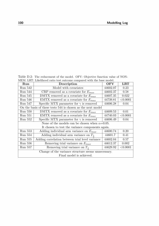
100 Modelling Log
Table D.2: The reducement of the model. OFV: Objective function value of NON-MEM. LRT: Likelihood ratio test outcome compared with the base model.
Run Description OFV LRTRun 542 Model with covariates 44602.07 0.23Run 544 CRP removed as a covariate for Emax 44602.37 0.58Run 545 DMTX removed as a covariate for Emax 44607.35 0.022Run 546 EMTX removed as a covariate for Emax 44739.81 <0.0001Run 547 Specific MTX parameter for γ is removed 44606.28 0.04On the basis of these tests 544 is chosen as the next modelRun 550 DMTX removed as a covariate for Emax 44609.53 0.01Run 551 EMTX removed as a covariate for Emax 44740.03 <0.0001Run 552 Specific MTX parameter for γ is removed 44606.49 0.04
None of the models can be chosen when α=0.05.It chosen to test the variance components again.
Run 553 Adding individual arm variance on Emax 44600.74 0.20Run 554 Adding individual arm variance on T 1
244601.7 0.41
Run 555 Adding correlation between trial level variance 44602.04 0.57Run 556 Removing trial variance on Emax 44612.37 0.002Run 557 Removing trial variance on T 1
244629.92 <0.0001
Change of the variance structure seems unnecessary.Final model is achieved.

101
Figure D.1: The final fit of the binomial model. The blue line is the typical value ofthe treatment and the red line is the individually fitted values.
Figure D.2: The final fit of the binomial model. The blue line is the typical value ofthe treatment and the red line is the individually fitted values.

102 Modelling Log
Figure D.3: The final fit of the binomial model. The blue line is the typical value ofthe treatment and the red line is the individually fitted values.
Figure D.4: The final fit of the binomial model. The blue line is the typical value ofthe treatment and the red line is the individually fitted values.

103
Figure D.5: The final fit of the binomial model. The blue line is the typical value ofthe treatment and the red line is the individually fitted values.
Figure D.6: The final fit of the binomial model. The blue line is the typical value ofthe treatment and the red line is the individually fitted values.

104 Modelling Log
Figure D.7: The final fit of the binomial model. The blue line is the typical value ofthe treatment and the red line is the individually fitted values.

Appendix E
Assumption Tests
In this part of the apendix the assumption tests for the ACR50 binomial modelis shown. The checks are performed in accordance with [51]. Assumption 1,2, 4, 6, 8, 15, 16 The sections do not include all the figures that were made,but only a selection. The test for the ACR20 and ACR70 binomial models arelocated on the Appendix CD. Assumption 3. Error-free sampling times.This assumption is tested by randomly increasing or decreasing the time ofall the data by a number of weeks taken from a random uniform distributionbetween -1 and 1 week. Running a NONMEM run over the new data gives theoutput given in Table E.1.
As seen in Table E.1 all the new estimates for the jittered data set are similarto the the estimates of the final model.Assumption 5. Model adequate despite data exlusion.This assumption was checked by removing all trials one by one from the dataset and then running the model again. This procedure produced the Figure E.1,E.2, E.3, E.4, and E.5. In the figure the trials are displayed against a number.The number signifies the trial taken out. The trials are numbered according tothe following list.
1. Abe2005
2. ERA2000

106 Assumption Tests
Table E.1: Estimates of the new run with a jittered time points from -1 to 1 weekalong with the original estimates. The numbers given in paranthesis indicate the95 % confidence interval of the estimates according to the standard errors providedby NONMEM. ∗: The parameters are still logit transformed. †: The parameter isexponentially multiplied on T 1
2.
Parameter Final model Jittered time modelEmax Placebo (%) 13.6 13.8
Emax MTX treatment (%) 43.6 44.3Emax Adalimumab (%) 42.8 44.5
Recommended doseEmax Adalimumab (%) 36.6 38.6
Low doseEmax Adalimumab (%) 50.1 52.4
High doseEmax Etanercept (%) 53.0 56.0Recommended doseEmax Etanercept (%) 40.4 43.0
Low doseEmax Infliximab (%) 39.2 40.3Recommended doseEmax Infliximab (%) 44.2 45.7
High doseT 1
2Placebo & MTX (Weeks) 9.30 8.92T 1
2Anti-TNFα (Weeks) 6.52 6.89
γ Placebo 1.61 1.52γ MTX 2.10 2.00
γ Anti-TNFα 1.24 1.14Emax covariate for 0.840 0.880
MTX effect on Anti-TNFα∗
Emax covariate for -0.586 -0.656halt of MTX treatment∗
Variance of random 8.33 ·10−2 7.99 ·10−2
component on E∗maxVariance of random 0.108 0.149component on T †1
2

107
3. PREMIER2006
4. STAR2003
5. Keystone2004Ada
6. Keystone2004Eta
7. Kim2007
8. TEMPO2004
9. ATTRACT1999
10. CHANGE2008
11. Moreland1999
12. ASPIRE2004
13. Putte2003
14. Putte2004
15. Weinblatt1999
16. ARMADA2003
17. START2006
18. ATTEST2008
19. Taylor2004
20. Zhang2006
In the figure it is seen that the parameters evidently changes values when someof trials are taken out of the data. Trial 2 and 8 corresponding to ERA2000and TEMPO2004 makes the biggest differences for the parameter values. Thisis evidently because of the large amount patients in the trials and the param-eter values are highly dependent upon those trials because they are the onlyones expressing this kind of treatment. This suggests that including the smallertrials does not impact the outcome. It should be noted that every model runwas succesfull without error messages except exclusion of the ASPIRE2004 trialwhich gave the message:0INVERSE COVARIANCE MATRIX SET TO RS*R, WHERE S* IS A PSEUDOINVERSE OF SBut it still produced reasonable estimates and standard errors.

108 Assumption Tests
Figure E.1: The impact of data exclusion upon the parameters for Emax of placebo,MTX treatment, adalimumab at recommended dose and adalimumab at low dose. Thewhiskers signify the 95 % confidence interval. The red line is the final model estimate.The numbers on the x-axis signfy trial removed from the data set. The 21st is thefinal model estimate.
Figure E.2: The impact of data exclusion upon the parameters for Emax of adalimu-mab at high dose, etanercept at both doses and infliximab at recommended dose. Thewhiskers signify the 95 % confidence interval. The red line is the final model estimate.The numbers on the x-axis signfy trial removed from the data set. The 21st is thefinal model estimate.

109
Figure E.3: The impact of data exclusion upon the parameters for Emax of infliximabat high dose, T 1
2for placebo, MTX treatment and TNF-α inhibitor treatment. The
whiskers signify the 95 % confidence interval. The red line is the final model estimate.The numbers on the x-axis signfy trial removed from the data set. The 21st is thefinal model estimate.
Figure E.4: The impact of data exclusion upon the parameters for the Emax covariatesof MTX treatment initiation and termination. The whiskers are signify the 95 %confidence interval. The red line is the final model estimate. The numbers on thex-axis signfy trial removed from the data set. The 21st is the final model estimate.

110 Assumption Tests
Figure E.5: The impact of data exclusion upon the parameter estimate for the vari-ance of Emax and T 1
2. The whiskers are signify the 95 % confidence interval. The red
line is the final model estimate. The numbers on the x-axis signfy trial removed fromthe data set. The 21st is the final model estimate.
Assumption 7. Adequate Structural model The population residuals, i.e.the residuals without the trial random effects, and the individual residuals, i.e.the residuals with the trial random effects, are shown against their respectivetime and prediction, shown in Figure E.6.
It is seen that there is no major model specifications problems in the Figure E.6.The Pearson’s residuals are of course higher when only looking at populationpredicted values and not accounting for differences in the population recruited.
It seems that the model has some troubles with high residuals coming fromthe CHANGE2008 study with adalimumab at normal dose and TEMPO2004at MTX and ARMADA with adalimumab at a normal dose which all havestandardised residuals above 2.5. The two first are coming from the first timepoint, so maybe it is not such a big problem because the model fits nicely to therest of the points. With the last one, the model clearly undershoots the data.This has a negative influence on adalimumab and care must be taken to this

111
Figure E.6: The population and individual arm residuals against their respective timeand prediciton.
estimate. Maybe a model that only includes half year data would be better.Assumption 9. Adequate covariate model building strategy
This assumption was checked by looking at the individual trial estimates forrandom effects with base and final model. It was checked and Figure E.7 andE.8 illustrates two of the covariates.It is seen that the variance components gets smaller and there is only one foreach trial, because the individual arm random coefficient has been removed.
Assumption 10. Shapes of covariate relationships are appropriate
All the covariates that were included in the end were categorical so they werenot tested. The numerical covariates were plotted in Figure E.9 against theirrespective EMAX values to see if there was some systematic tendency.
Looking at Figure E.9 it can be seen that there is no problems with the numericalcovariates.Assumption 11. Abscence of interactions.

112 Assumption Tests
Figure E.7: The trial random effect values for Emax of the base and final modelplotted against the mean duration of disease for the patients of the trial arm.
Figure E.8: The trial random effect values for Emax of the base and final modelplotted against the mean baseline serum C-reactive protein.

113
Figure E.9: The numerival covariates of the trial arms against their respective Emaxvalue.
In Figure E.10 the random effects are plotted against their respective drugdivided by MTX initiation.
The model sufficiently fits as the interaction between drug and MTX effect looks.There are too few trials to say anything about other interactions, there is notenough trials.
When looking at the MTX treated patients there seems to be some inconsis-tency. For TEMPO2004 infliximab is lower than the rest along with its MTXtreatment. There is apparently something different about TEMPO2004. Maybeit is because they allow their patients to receive 3 times MTX before enlisting,which means that they are not initiating the treatment in the same way as theother trials.
Assumption 12. Distribution of individual parameters adequatelymodeled.
The normal distribution of the random effects were checked by histograms andQQ-plots for both the random effects of Emax and T 1
2and they are seen in

114 Assumption Tests
Figure E.10: Plot of the interactions between MTX effect and drug. 1, 2, 3 and 4correspond to placebo, adalimumab, etanercept and infliximab respectively.
Figure E.11.
As it is seen in Figure E.11 the distribution of the trial variance componentsseems to be normal distributed comparing to the fact that there is only 20 trials.
Assumption 13. Heteroscedacity in variance models appropriately ac-counted for.Heteroscedacity of the models were visualised looking at the values of the ran-dom effects for Emax against the typical value of the parameter. This could beseen in Figure E.12.
As it can be seen from E.12 the heteroscedacity seems to have some problems,but compared to number of trials it is appropriately accounted for.
Assumption 14. Appropriate correlation structure in interindividualand interoccasion variability
To see assess whether this assumption was violated the Emax and T 12
randomeffects were plotted against each other, as seen in Figure E.13.

115
Figure E.11: The QQ-plot and histogram of both the Emax and T 12
random effects.
As seen in Figure E.13 no apparent correlation structure between the two vari-ance components.Assumption 17. Adequate shape of the distribution of residual errors.This assumption was checked be looking at the weighted residuals in a histogramand in a qq-plot, seen in Figure E.14.
As seen from Figure E.14 the residuals seem to be approximately binomiallydistributed. There is 3 points of large positive error which has already beenmentioned. The mean of the residuals is negative even though the largest valuesare positive. This suggests leaving out these points. The variation is smallerthan one indicating that the residuals do no not vary as much as the theoreticalbinomial distribution.Assumption 18. Independence of residual errors.To assess the independence of the residuals a continuous and discrete covariancefunction were made for the residuals as seen in Figure E.15.
The first two upper plots of Figure E.15 illustrate the problem with the data

116 Assumption Tests
Figure E.12: The value of the random effects for Emax against the absolute of thetypical values.
sampling. The continuous data shows no consensus picture on autocorrelation.When looking at the lower two figure with discrete lags a more consistent pictureevolves.
The first 2 discrete lags seems to adequately fitted but the covariance gets morenegative until the lag of 5. Hereafter the covariance increases until lag 9 andthen decreases dramatically at lag 10 to the largest negative value. Using anautoregressive model could maybe solve some of the problems as suggested in[51].
Assumption 18. Global minimum is found.
One standard error was both subtracted or added to each of the initial estimatesof the fixed effects. All final parameter estimates were the same for all runs.The plots are not shown.
Only the standard error changes for all the parameter estimates. The maximaldeviation is 0.3 from the orginal estimates of standard error for T 1
2of TNF-α
and placebo. It is when theta for etanercept at low dose is subtracted 1 standarderror. This suggests that one must be careful when using the standard errors of

117
Figure E.13: The value of the random effects plotted against each other.
NONMEM since those estimates changes dependent on the initial estimate.
E.0.5 Other tests
Shrinkage:
Shrinkage is a measure of the credibility of the random effects[52]. It indicatesthe amount of information about the variablity which is contained in data set.
Shrinkage of the all the components of variation was inspected.For b1, the vari-ation of Emax, the shrinkage was 10 %, for b2, the variation of T 1
2, 24 % and
for ε 13 %. There is problem with b2 which suggests that the data contain littleinformation about this parameter.
Population and individual predictions
Some tests were also suggested by [27]. Among these were the observed versuspredicted both in number of responders and proportions as seen in Figure E.16.
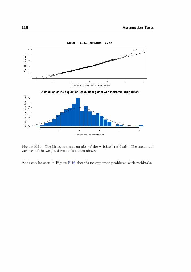
118 Assumption Tests
Figure E.14: The histogram and qq-plot of the weighted residuals. The mean andvariance of the weighted residuals is seen above.
As it can be seen in Figure E.16 there is no apparent problems with residuals.

119
Figure E.15: The discrete and continuous covariance function of the residuals.
Figure E.16: The population and individual predicted versus the observed valuesboth for proportions and number of responders.

120 Assumption Tests

Appendix F
PKPD-results
In this part of the appendix. The final results of the PKPD analysis for ACR20and ACR70 are shown.

122 PKPD-results
Figure F.1: The parameter estimates for the ACR20 and ACR70 binomial modelplotted against the values of outcomes value of the PKPD-analysis.

Bibliography
[1] Guidance for Industry: Clinical Development Programs for Drugs, De-vices, and Biological Products for the Treatment of Rheumatoid Arthritis(RA), pages 2–6, 11–24. U.S. Department of Health and Human ServicesFood and Drug Administration, Center for Drug Evaluation and Research(CDER), Center for Biologics Evaluation and Research (CBER), Centerfor Devices and Radiologic Health (CDRH), Feb 1999.
[2] REMICADETM (Infliximab) Patient Information., pages 1–3. CentocorInc., 2001.
[3] ENBRELTM (etanercept) Patient Information., pages 1–6. Amgen Inc,2003.
[4] HUMIRATM (adalimumab) Patient Information., pages 1–4. Abbott Lab-oratories, 2003.
[5] Remicade: SUMMARY OF PRODUCT CHARACTERISTICS, pages 28,40–45. EMEA, 2004.
[6] Enbrel: SUMMARY OF PRODUCT CHARACTERISTICS, pages 2–9,25–26. EMEA, 2005.
[7] European public assessment report: Remicade. summary for the public.EMEA, 2007.
[8] European public assessment report: Enbrel. summary for the public.EMEA, 2008.
[9] European public assessment report: Humira. summary for the public.EMEA, 2008.

124 BIBLIOGRAPHY
[10] Humira: SUMMARY OF PRODUCT CHARACTERISTICS, pages 2–9,26–27. EMEA, 2009.
[11] T. Abe, T. Takeuchi, N. Miyasaka, H. Hashimoto, H. Kondo, Y. Ichikawa,and I. Nagaya. A multicenter, double-blind, randomized, placebo con-trolled trial of infliximab combined with low dose methotrexate in japanesepatients with rheumatoid arthritis. J Rheumatol., 33(1):37–44, January2006.
[12] D. G. Altman, K. F. Schulz, D. Moher, M. Egger, F. Davidoff, D. El-bourne, P. C. Gøtzsche, T. Lang, and C. O. N. S. O. R. T. GROUP(Consolidated Standards of Reporting Trials). The revised consort state-ment for reporting randomized trials: explanation and elaboration. AnnIntern Med, 134(8):663–694, Apr 2001.
[13] D. M. Bates and D. G. Watts. Nonlinear Regression Analysis and ItsApplications, pages 1–231. Wiley, 1988.
[14] J. M. Bathon, R. W. Martin, R. M. Fleischmann, J. R. Tesser, M. H.Schiff, E. C. Keystone, M. C. Genovese, M. C. Wasko, L. W. Moreland,A. L. Weaver, J. Markenson, and B. K. Finck. A comparison of etanerceptand methotrexate in patients with early rheumatoid arthritis. N Engl JMed, 343(22):1586–1593, Nov 2000.
[15] S. L. Beal and L. B. Sheiner. NONMEM users guide. ICON, 1988.
[16] J. Berkson. Application of the logistic function to bio-assay. Journal ofthe American Statistical Association, 39(227):357–365, 1944.
[17] M. P. Bevilacqua and M. A. Gimbrone. Inducible endothelial functionsin inflammation and coagulation. Semin Thromb Hemost, 13(4):425–433,Oct 1987.
[18] H. Bliddal, L. Terslev, E. Qvistgaard, M. Konig, C.C. Holm, H. Rogind,M. Boesen, B. nneskiold Samsoe, and S. Torp-Pedersen. A randomized,controlled study of a single intra-articular injection of etanercept or gluco-corticosteroids in patients with rheumatoid arthritis. Scand.J Rheumatol.,35(5):341–345, September 2006.
[19] Brendan F Boyce, Edward M Schwarz, and Lianping Xing. Osteoclastprecursors: cytokine-stimulated immunomodulators of inflammatory bonedisease. Curr Opin Rheumatol, 18(4):427–432, Jul 2006.
[20] Ferdinand C Breedveld, Michael H Weisman, Arthur F Kavanaugh, Stan-ley B Cohen, Karel Pavelka, Ronald van Vollenhoven, John Sharp, John LPerez, and George T Spencer-Green. The premier study: A multicen-ter, randomized, double-blind clinical trial of combination therapy with

BIBLIOGRAPHY 125
adalimumab plus methotrexate versus methotrexate alone or adalimumabalone in patients with early, aggressive rheumatoid arthritis who had nothad previous methotrexate treatment. Arthritis Rheum, 54(1):26–37, Jan2006.
[21] Goran Brostrom. glmmML Reference Manual. R Project for StatisticalComputing, 0.81-4 edition, 2 2009.
[22] R. A. Bunning and R. G. Russell. The effect of tumor necrosis factor alphaand gamma-interferon on the resorption of human articular cartilage andon the production of prostaglandin e and of caseinase activity by humanarticular chondrocytes. Arthritis Rheum, 32(6):780–784, Jun 1989.
[23] P. Charles, M. J. Elliott, D. Davis, A. Potter, J. R. Kalden, C. Antoni,F. C. Breedveld, J. S. Smolen, G. Eberl, K. deWoody, M. Feldmann, andR. N. Maini. Regulation of cytokines, cytokine inhibitors, and acute-phase proteins following anti-tnf-alpha therapy in rheumatoid arthritis. JImmunol, 163(3):1521–1528, Aug 1999.
[24] Hyon K Choi, Miguel A Hernan, John D Seeger, James M Robins, andFrederick Wolfe. Methotrexate and mortality in patients with rheumatoidarthritis: a prospective study. Lancet, 359(9313):1173–1177, Apr 2002.
[25] C. Christodoulou and E. H. Choy. Joint inflammation and cytokine inhi-bition in rheumatoid arthritis. Clin Exp Med, 6(1):13–19, Mar 2006.
[26] C. P. Chung, J. L. Thompson, G. G. Koch, I. Amara, V. Strand, andT. Pincus. Are american college of rheumatology 50to 20arthritis clinicaltrials reported since 1997? a meta-analysis of discriminant capacities. AnnRheum Dis, 65(12):1602–1607, Dec 2006.
[27] D. Collett. Modelling binary data, pages 1–276. CRC Press, 2002.
[28] J. S. Cramer. The origins and development of the logit model. 2003.
[29] M. Davidian and D. M. Giltinan. Nonlinear models for repeated measure-ment data, pages 1–190. CRC Press, 1995.
[30] J. L. Decker, D. G. Malone, B. Haraoui, S. M. Wahl, L. Schrieber, J. H.Klippel, A. D. Steinberg, and R. L. Wilder. Nih conference. rheumatoidarthritis: evolving concepts of pathogenesis and treatment. Ann InternMed, 101(6):810–824, Dec 1984.
[31] A. den Broeder, L.B.A. van de Putte, R. Rau, M. Schattenkirchner,P.L.C.M. van Riel, O. Sander, C. Binder, H. Fenner, Y. Bankmann, R. Ve-lagapudi, J. Kempeni, and H. Kupper. A single dose, placebo controlledstudy of the fully human anti-tumor necrosis factor-alpha antibody ada-limumab (d2e7) in patients with rheumatoid arthritis. J.RHEUMATOL.,29(11):2288–2298, 2002.

126 BIBLIOGRAPHY
[32] Adrian Dunne. Icon development solutions: Binary and categorical datamodeling, analysis & simulation using nonmem. course material. Globo-max, LLC, June 2004.
[33] P. Emery, F.C. Breedveld, S. Hall, P. Durez, D.J. Chang, D. Robertson,A. Singh, R.D. Pedersen, A.S. Koenig, and B. Freundlich. Comparison ofmethotrexate monotherapy with a combination of methotrexate and etan-ercept in active, early, moderate to severe rheumatoid arthritis (comet): arandomised, double-blind, parallel treatment trial. Lancet, 372(9636):375–382, August 2008.
[34] R. M. Enoka. Neuromechanics of Human Movement 3rd edition, pages211–219. Human Kinetics, 2002.
[35] M. Feldmann and R. N. Maini. Anti-tnf alpha therapy of rheumatoidarthritis: what have we learned? Annu Rev Immunol, 19:163–196, 2001.
[36] D. T. Felson, J. J. Anderson, M. Boers, C. Bombardier, M. Chernoff,B. Fried, D. Furst, C. Goldsmith, S. Kieszak, and R. Lightfoot. Theamerican college of rheumatology preliminary core set of disease activitymeasures for rheumatoid arthritis clinical trials. the committee on out-come measures in rheumatoid arthritis clinical trials. Arthritis Rheum,36(6):729–740, Jun 1993.
[37] D. T. Felson, J. J. Anderson, M. Boers, C. Bombardier, D. Furst, C. Gold-smith, L. M. Katz, R. Lightfoot, H. Paulus, and V. Strand. American col-lege of rheumatology. preliminary definition of improvement in rheumatoidarthritis. Arthritis Rheum, 38(6):727–735, Jun 1995.
[38] D. T. Felson, J. J. Anderson, M. L. Lange, G. Wells, and M. P. LaValley.Should improvement in rheumatoid arthritis clinical trials be defined asfifty percent or seventy percent improvement in core set measures, ratherthan twenty percent? Arthritis Rheum, 41(9):1564–1570, Sep 1998.
[39] D. E. Furst, F. C. Breedveld, J. R. Kalden, J. S. Smolen, G. R. Burmester,J. Sieper, P. Emery, E. C. Keystone, M. H. Schiff, P. Mease, P. L C Mvan Riel, R. Fleischmann, M. H. Weisman, and M. E. Weinblatt. Updatedconsensus statement on biological agents for the treatment of rheumaticdiseases, 2007. Ann Rheum Dis, 66 Suppl 3:iii2–ii22, Nov 2007.
[40] Daniel E Furst, Robert Wallis, Michael Broder, and David O Beenhouwer.Tumor necrosis factor antagonists: different kinetics and/or mechanismsof action may explain differences in the risk for developing granulomatousinfection. Semin Arthritis Rheum, 36(3):159–167, Dec 2006.
[41] D.E. Furst, M.H. Schiff, R.M. Fleischmann, V. Strand, C.A. Birbara,D. Compagnone, S.A. Fischkoff, and E.K. Chartash. Adalimumab, a fully

BIBLIOGRAPHY 127
human anti tumor necrosis factor-alpha monoclonal antibody, and con-comitant standard antirheumatic therapy for the treatment of rheuma-toid arthritis: results of star (safety trial of adalimumab in rheumatoidarthritis). J Rheumatol., 30(12):2563–2571, December 2003.
[42] J. Gabrielsson and D. Weiner. Pharmacokinetic/pharmacodynamic DataAnalysis: Concepts and Applications, pages 1–257. Taylor & Francis, 2000.
[43] Mark C Genovese, Joan M Bathon, Richard W Martin, Roy MFleischmann, John R Tesser, Michael H Schiff, Edward C Keystone,Mary Chester Wasko, Larry W Moreland, Arthur L Weaver, JosephMarkenson, Grant W Cannon, George Spencer-Green, and Barbara KFinck. Etanercept versus methotrexate in patients with early rheumatoidarthritis: two-year radiographic and clinical outcomes. Arthritis Rheum,46(6):1443–1450, June 2002.
[44] Yvonne P M Goekoop-Ruiterman, Jeska K de Vries-Bouwstra, Cornelia FAllaart, Pit J S M Kerstens, Bernard A M Grillet, Mike H de Jager,K. Huub Han, Irene Speyer, Peter A H M van der Lubbe, Patrick E H Seys,Ferdinand C Breedveld, and Ben A C Dijkmans. Patient preferences fortreatment: report from a randomised comparison of treatment strategiesin early rheumatoid arthritis (best trial). Ann Rheum Dis, 66(9):1227–1232, Sep 2007.
[45] J. P. T. Higgins and S. Green, editors. Cochrane Handbook for SystematicReviews of Interventions version 4.2.6. The Cochrane Collaboration, 2006.
[46] M. C. Hochberg, J. K. Tracy, M. Hawkins-Holt, and R. H. Flores. Com-parison of the efficacy of the tumour necrosis factor alpha blocking agentsadalimumab, etanercept, and infliximab when added to methotrexate inpatients with active rheumatoid arthritis. Ann Rheum Dis, 62 Suppl2:ii13–ii16, Nov 2003.
[47] Insightful. S-PLUS 7 Enterprise Developer Users Guide, 2007.
[48] M. Jit, B. Henderson, M. Stevens, and R. M. Seymour. Tnf-alpha neu-tralization in cytokine-driven diseases: a mathematical model to accountfor therapeutic success in rheumatoid arthritis but therapeutic failurein systemic inflammatory response syndrome. Rheumatology (Oxford),44(3):323–331, Mar 2005.
[49] Alyssa K Johnsen, Michael H Schiff, Philip J Mease, Larry W Moreland,Agnes L Maier, Jonathan S Coblyn, Simon M Helfgott, Jonathan A Leff,and Michael E Weinblatt. Comparison of 2 doses of etanercept (50 vs 100mg) in active rheumatoid arthritis: a randomized double blind study. JRheumatol, 33(4):659–664, Apr 2006.

128 BIBLIOGRAPHY
[50] R. A. Johnson. Miller and Freunds Probability and Statistics for Engi-neers, pages 238–244. Pearson Prentice Hall, 7 edition, 2005.
[51] M. O. Karlsson, E. N. Jonsson, C. G. Wiltse, and J. R. Wade. Assumptiontesting in population pharmacokinetic models: illustrated with an analy-sis of moxonidine data from congestive heart failure patients. J Pharma-cokinet Biopharm, 26(2):207–246, Apr 1998.
[52] M. O. Karlsson and R. M. Savic. Diagnosing model diagnostics. ClinPharmacol Ther, 82(1):17–20, Jul 2007.
[53] A. Kavanaugh, E.W. St Clair, W.J. McCune, T. Braakman, and P. Lipsky.Chimeric anti-tumor necrosis factor-alpha monoclonal antibody treatmentof patients with rheumatoid arthritis receiving methotrexate therapy. JRheumatol., 27(4):841–850, April 2000.
[54] Zehra Kaymakcalan, Paul Sakorafas, Sahana Bose, Susanne Scesney,Limin Xiong, Denise Karaoglu Hanzatian, Jochen Salfeld, and Eric HSasso. Comparisons of affinities, avidities, and complement activation ofadalimumab, infliximab, and etanercept in binding to soluble and mem-brane tumor necrosis factor. Clin Immunol, Jan 2009.
[55] E.C. Keystone, A.F. Kavanaugh, J.T. Sharp, H. Tannenbaum, Y. Hua,L.S. Teoh, S.A. Fischkoff, and E.K. Chartash. Radiographic, clinical, andfunctional outcomes of treatment with adalimumab (a human anti-tumornecrosis factor monoclonal antibody) in patients with active rheuma-toid arthritis receiving concomitant methotrexate therapy - a randomized,placebo-controlled, 52-week trial. Arthritis and Rheumatism, 50(5):1400–1411, 2004.
[56] E.C. Keystone, M.H. Schiff, J.M. Kremer, S. Kafka, M. Lovy, T. DeVries,and D.J. Burge. Once-weekly administration of 50 mg etanercept in pa-tients with active rheumatoid arthritis - results of a multicenter, random-ized, double-blind, placebo-controlled trial. Arthritis and Rheumatism,50(2):353–363, 2004.
[57] H.Y. Kim, S.K. Lee, Y.W. Song, D.H. Yoo, E.M. Koh, B. Yoo, and A. Luo.A randomized, double-blind, placebo-controlled, phase iii study of thehuman anti-tumor necrosis factor antibody adalimumab administered assubcutaneous injections in korean rheumatoid arthritis patients treatedwith methotrexate. APLAR J.RHEUMATOL., 10(1):9–16, 2007.
[58] Lars Klareskog, Desiree van der Heijde, Julien P de Jager, AndrewGough, Joachim Kalden, Michel Malaise, Emilio Martın Mola, KarelPavelka, Jacques Sany, Lucas Settas, Joseph Wajdula, Ronald Pedersen,Saeed Fatenejad, Marie Sanda, T. E. M. P. O. (Trial of Etanercept, andMethotrexate with Radiographic Patient Outcomes) study investigators.

BIBLIOGRAPHY 129
Therapeutic effect of the combination of etanercept and methotrexatecompared with each treatment alone in patients with rheumatoid arthri-tis: double-blind randomised controlled trial. Lancet, 363(9410):675–681,Feb 2004.
[59] P. A. Klimiuk, S. Sierakowski, R. Latosiewicz, J. P. Cylwik, B. Cylwik,J. Skowronski, and J. Chwiecko. Circulating tumour necrosis factor alphaand soluble tumour necrosis factor receptors in patients with differentpatterns of rheumatoid synovitis. Ann Rheum Dis, 62(5):472–475, May2003.
[60] L. E. Kristensen, R. Christensen, H. Bliddal, P. Geborek, B. Danneskiold-Samsøe, and T. Saxne. The number needed to treat for adalimumab,etanercept, and infliximab based on acr50 response in three randomizedcontrolled trials on established rheumatoid arthritis: a systematic litera-ture review. Scand J Rheumatol, 36(6):411–417, 2007.
[61] R. L. Lalonde, K. G. Kowalski, M. M. Hutmacher, W. Ewy, D. J. Nichols,P. A. Milligan, B. W. Corrigan, P. A. Lockwood, S. A. Marshall, L. J.Benincosa, T. G. Tensfeldt, K. Parivar, M. Amantea, P. Glue, H. Koide,and R. Miller. Model-based drug development. Clin Pharmacol Ther,82(1):21–32, Jul 2007.
[62] J.L. Lan, S.J. Chou, D.Y. Chen, Y.H. Chen, T.Y. Hsieh, and M. Young.A comparative study of etanercept plus methotrexate and methotrexatealone in taiwanese patients with active rheumatoid arthritis: A 12-week,double-blind, randomized, placebo-controlled study. Journal of the For-mosan Medical Association, 103(8):618–623, 2004.
[63] D. M. Lee and M. E. Weinblatt. Rheumatoid arthritis. Lancet,358(9285):903–911, Sep 2001.
[64] Howard Lee, Hui C Kimko, Mark Rogge, Diane Wang, Ivan Nestorov,and Carl C Peck. Population pharmacokinetic and pharmacodynamicmodeling of etanercept using logistic regression analysis. Clin PharmacolTher, 73(4):348–365, Apr 2003.
[65] M. L. Lindstrom and D. M. Bates. Nonlinear mixed effects models forrepeated measures data. Biometrics, 46(3):673–687, Sep 1990.
[66] P.E. Lipsky, D.M. Van Der Heijde, E.W. St Clair, D.E. Furst, F.C.Breedveld, J.R. Kalden, J.S. Smolen, M. Weisman, P. Emery, M. Feld-mann, G.R. Harriman, and R.N. Maini. Infliximab and methotrexate inthe treatment of rheumatoid arthritis. anti-tumor necrosis factor trial inrheumatoid arthritis with concomitant therapy study group. N.Engl.JMed., 343(22):1594–1602, November 2000.

130 BIBLIOGRAPHY
[67] R. Maini, E.W. St Clair, F. Breedveld, D. Furst, J. Kalden, M. Weis-man, J. Smolen, P. Emery, G. Harriman, M. Feldmann, and P. Lip-sky. Infliximab (chimeric anti-tumour necrosis factor alpha monoclonalantibody) versus placebo in rheumatoid arthritis patients receiving con-comitant methotrexate: a randomised phase iii trial. attract study group.Lancet, 354(9194):1932–1939, December 1999.
[68] R.N. Maini, F.C. Breedveld, J.R. Kalden, J.S. Smolen, D. Davis, J.D.Macfarlane, C. Antoni, B. Leeb, M.J. Elliott, J.N. Woody, T.F. Schaible,and M. Feldmann. Therapeutic efficacy of multiple intravenous infusions ofanti-tumor necrosis factor alpha monoclonal antibody combined with low-dose weekly methotrexate in rheumatoid arthritis. Arthritis and Rheuma-tism, 41(9):1552–1563, 1998.
[69] N. Miyasaka. Clinical investigation in highly disease-affected rheumatoidarthritis patients in japan with adalimumab applying standard and gen-eral evaluation: The change study. MOD.RHEUMATOL., 18(3):252–262,2008.
[70] Jonas Bech Møller. Stochastic Models and Methods to Characterise theGlucose/Insulin System, page 33. Department of Informatics and Mathe-matical Modelling (IMM), DTU, 2008.
[71] L.W. Moreland, S.W. Baumgartner, M.H. Schiff, E.A. Tindall, R.M.Fleischmann, A.L. Weaver, R.E. Ettlinger, S. Cohen, W.J. Koopman,K. Mohler, M.B. Widmer, and C.M. Blosch. Treatment of rheumatoidarthritis with a recombinant human tumor necrosis factor receptor (p75)-fc fusion protein. N.Engl.J Med., 337(3):141–147, July 1997.
[72] L.W. Moreland, M.H. Schiff, S.W. Baumgartner, E.A. Tindall, R.M. Fleis-chmann, K.J. Bulpitt, A.L. Weaver, E.C. Keystone, D.E. Furst, P.J.Mease, E.M. Ruderman, D.A. Horwitz, D.G. Arkfeld, L. Garrison, D.J.Burge, C.M. Blosch, M.L.M. Lange, N.D. McDonnell, and M.E. Wein-blatt. Etanercept therapy in rheumatoid arthritis - a randomized, con-trolled trial. Annals of Internal Medicine, 130(6):478–+, 1999.
[73] J. M. Mullin and K. V. Snock. Effect of tumor necrosis factor on epithelialtight junctions and transepithelial permeability. Cancer Res, 50(7):2172–2176, Apr 1990.
[74] Ivan Nestorov. Clinical pharmacokinetics of tnf antagonists: how do theydiffer? Semin Arthritis Rheum, 34(5 Suppl1):12–18, Apr 2005.
[75] R. M. Nixon, N. Bansback, and A. Brennan. Using mixed treatmentcomparisons and meta-regression to perform indirect comparisons to esti-mate the efficacy of biologic treatments in rheumatoid arthritis. Stat Med,26(6):1237–1254, Mar 2007.

BIBLIOGRAPHY 131
[76] T. J. Nowak and A. G. Handford. Patophysiology: Concepts and Applica-tions for Health Care Professionals, pages 28–49, 494–500. McGraw-Hill,2004.
[77] James R O’Dell. Therapeutic strategies for rheumatoid arthritis. N EnglJ Med, 350(25):2591–2602, Jun 2004.
[78] K. Pfizenmaier, M. Kronke, P. Scheurich, and G. A. Nagel. Tumor necrosisfactor (tnf) alpha: control of tnf-sensitivity and molecular mechanisms oftnf-mediated growth inhibition. Blut, 55(1):1–10, Jul 1987.
[79] J. C. Pinheiro and D. M. Bates. Mixed-effects models in S and S-PLUS,pages 273–276, 305–336. Springer, 2000.
[80] J. C. Pinhero and D. M. Bates. Approximations to the log-likelihoodfunction in the nonlinear mixed-effects model. Journal of Computationaland Graphical Statistics, 4(1):12–35, 1995.
[81] J. Pitman. Probability, page 430. Springer, 1993.
[82] M.A. Quinn, P.G. Conaghan, P.J. O’Connor, Z. Karim, A. Greenstein,A. Brown, C. Brown, A. Fraser, S. Jarret, and P. Emery. Very early treat-ment with infliximab in addition to methotrexate in early, poor-prognosisrheumatoid arthritis reduces magnetic resonance imaging evidence of syn-ovitis and damage, with sustained benefit after infliximab withdrawal -results from a twelve-month randomized, double-blind, placebo-controlledtrial. Arthritis and Rheumatism, 52(1):27–35, 2005.
[83] Mahboob U Rahman, Ingrid Strusberg, Piet Geusens, Alberto Berman,David Yocum, Daniel Baker, Carrie Wagner, John Han, and ReneWesthovens. Double-blinded infliximab dose escalation in patients withrheumatoid arthritis. Ann Rheum Dis, 66(9):1233–1238, Sep 2007.
[84] R. Rau, S. Simianer, P.L.C.M. van Riel, L.B.A. van de Putte, K. Kruger,M. Schattenkirchner, C.F. Allaart, F.C. Breedveld, J. Kempeni, K. Beck,and H. Kupper. Rapid alleviation of signs and symptoms of rheumatoidarthritis with intravenous or subcutaneous administration of adalimumabin combination with methotrexate. Scandinavian Journal of Rheumatol-ogy, 33(3):145–153, 2004.
[85] Kenneth G Saag, Gim Gee Teng, Nivedita M Patkar, Jeremy Anun-tiyo, Catherine Finney, Jeffrey R Curtis, Harold E Paulus, Amy Mu-dano, Maria Pisu, Mary Elkins-Melton, Ryan Outman, Jeroan J Alli-son, Maria Suarez Almazor, S. Louis Bridges, W. Winn Chatham, MarcHochberg, Catherine MacLean, Ted Mikuls, Larry W Moreland, JamesO’Dell, Anthony M Turkiewicz, Daniel E Furst, and American College

132 BIBLIOGRAPHY
of Rheumatology. American college of rheumatology 2008 recommen-dations for the use of nonbiologic and biologic disease-modifying an-tirheumatic drugs in rheumatoid arthritis. Arthritis Rheum, 59(6):762–784, Jun 2008.
[86] P. Scheurich, B. Thoma, U. Ucer, and K. Pfizenmaier. Immunoregulatoryactivity of recombinant human tumor necrosis factor (tnf)-alpha: induc-tion of tnf receptors on human t cells and tnf-alpha-mediated enhancementof t cell responses. J Immunol, 138(6):1786–1790, Mar 1987.
[87] M. Schiff, M. Keiserman, C. Codding, S. Songcharoen, A. Berman,S. Nayiager, C. Saldate, T. Li, R. Aranda, J.C. Becker, C. Lin, P.L.N.Cornet, and M. Dougados. Efficacy and safety of abatacept or infliximabvs placebo in attest: a phase iii, multi-centre, randomised, double-blind,placebo-controlled study in patients with rheumatoid arthritis and an in-adequate response to methotrexate. Annals of the Rheumatic Diseases,67(8):1096–1103, 2008.
[88] T. V. Schroeder, S. Schulze, J. Hilsted, and J. Aldershvile. Basisbog iMedicin og Kirurgi 2nd edition, pages 271–277. Munksgaard Danmark,2003.
[89] R. R. Seely, T. D. Stephens, and P. Tate. Anatomy & Physiology 6thedition, pages 241–266. McGraw-Hill, 2006.
[90] R. Segal, M. Yaron, and B. Tartakovsky. Methotrexate: mechanism ofaction in rheumatoid arthritis. Semin Arthritis Rheum, 20(3):190–200,Dec 1990.
[91] D. J. Shealy and S. Visvanathan. Anti-tnf antibodies: lessons from thepast, roadmap for the future. Handb Exp Pharmacol, (181):101–129, 2008.
[92] J. Bruce Smith and Mark K Haynes. Rheumatoid arthritis–a molecularunderstanding. Ann Intern Med, 136(12):908–922, Jun 2002.
[93] J. S. Smolen, C. Han, M. Bala, R. N. Maini, J. R. Kalden, D. van derHeijde, F. C. Breedveld, D. E. Furst, P. E. Lipsky, and A. T. T. R. A.C. T. Study Group. Evidence of radiographic benefit of treatment withinfliximab plus methotrexate in rheumatoid arthritis patients who hadno clinical improvement: a detailed subanalysis of data from the anti-tumor necrosis factor trial in rheumatoid arthritis with concomitant ther-apy study. Arthritis Rheum, 52(4):1020–1030, Apr 2005.
[94] Josef S Smolen, Daniel Aletaha, Marcus Koeller, Michael H Weisman, andPaul Emery. New therapies for treatment of rheumatoid arthritis. Lancet,370(9602):1861–1874, Dec 2007.

BIBLIOGRAPHY 133
[95] J.S. Smolen, D.M.F.M. van der Heijde, E.W. St Clair, P. Emery, J.M.Bathon, E. Keystone, R.N. Maini, J.R. Kalden, M. Schiff, D. Baker, C.L.Han, J. Han, M. Bala, and Study Grp Aspire. Predictors of joint dam-age in patients with early rheumatoid arthritis treated with high-dosemethotrexate with or without concomitant infliximab - results from theaspire trial. Arthritis and Rheumatism, 54(3):702–710, 2006.
[96] T. Sokka, B. Abelson, and T. Pincus. Mortality in rheumatoid arthritis:2008 update. Clin Exp Rheumatol, 26(5 Suppl 51):S35–S61, 2008.
[97] E. William St. Clair, Desiree M F M van der Heijde, Josef S Smolen, Ravin-der N Maini, Joan M Bathon, Paul Emery, Edward Keystone, MichaelSchiff, Joachim R Kalden, Ben Wang, Kimberly Dewoody, RobertaWeiss, Daniel Baker, and Active-Controlled Study of Patients Receiv-ing Infliximab for the Treatment of Rheumatoid Arthritis of Early On-set Study Group. Combination of infliximab and methotrexate therapyfor early rheumatoid arthritis: a randomized, controlled trial. ArthritisRheum, 50(11):3432–3443, Nov 2004.
[98] E.W. St Clair, C.L. Wagner, A.A. Fasanmade, B. Wang, T. Schaible,A. Kavanaugh, and E.C. Keystone. The relationship of serum infliximabconcentrations to clinical improvement in rheumatoid arthritis - resultsfrom attract, a multicenter, randomized, double-blind, placebo-controlledtrial. Arthritis and Rheumatism, 46(6):1451–1459, 2002.
[99] P.C. Taylor, A. Steuer, J. Gruber, D.O. Cosgrove, M.J.K. Blomley, P.A.Marsters, C.L. Wagner, C. McClinton, and R.N. Maini. Comparison ofultrasonographic assessment of synovitis and joint vascularity with radio-graphic evaluation in a randomized, placebo-controlled study of inflixi-mab therapy in early rheumatoid arthritis. Arthritis and Rheumatism,50(4):1107–1116, 2004.
[100] David Ternant and Gilles Paintaud. Pharmacokinetics and concentration-effect relationships of therapeutic monoclonal antibodies and fusion pro-teins. Expert Opin Biol Ther, 5 Suppl 1:S37–S47, Sep 2005.
[101] C. W. Tornøe. Population pharmacokinetic/pharmacodynamic modellingof the hypothalamic-pituitary-gonadal axis, chapter 4, pages 20–27. De-partment of Informatics and Mathematical Modelling (IMM), DTU, 2005.
[102] Christoffer W Tornøe, Henrik Agersø, Henrik A Nielsen, Henrik Madsen,and E. Niclas Jonsson. Pharmacokinetic/pharmacodynamic modelling ofgnrh antagonist degarelix: a comparison of the non-linear mixed-effectsprograms nonmem and nlme. J Pharmacokinet Pharmacodyn, 31(6):441–461, Dec 2004.

134 BIBLIOGRAPHY
[103] B.A. van de Putte, C. Atkins, M. Malaise, J. Sany, A.S. Russell, P.L.C.M.van Riel, L. Settas, J.W. Biljsma, S. Todesco, M. Dougados, P. Nash,P. Emery, N. Walter, M. Kaul, S. Fischkoff, and H. Kupper. Efficacy andsafety of adalimumab as monotherapy in patients with rheumatoid arthri-tis for whom previous disease modifying antirheumatic drug treatment hasfailed. Annals of the Rheumatic Diseases, 63(5):508–516, 2004.
[104] L.B. van de Putte, R. Rau, F.C. Breedveld, J.R. Kalden, M.G. Malaise,P.L. van Riel, M. Schattenkirchner, P. Emery, G.R. Burmester, H. Zeidler,H.M. Moutsopoulos, K. Beck, and H. Kupper. Efficacy and safety of thefully human anti-tumour necrosis factor alpha monoclonal antibody ada-limumab (d2e7) in dmard refractory patients with rheumatoid arthritis:a 12 week, phase ii study. Ann.Rheum.Dis., 62(12):1168–1177, December2003.
[105] van der Heijde D., L. Klareskog, M. Boers, R. Landewe, C. Codreanu,H.D. Bolosiu, R. Pedersen, and S. Fatenejad. Comparison of differentdefinitions to classify remission and sustained remission: 1 year temporesults. Ann.Rheum.Dis., 64(11):1582–1587, November 2005.
[106] van der Heijde D., L. Klareskog, V. Rodriguez-Valverde, C. Codreanu,H. Bolosiu, J. Melo-Gomes, J. Tornero-Molina, J. Wajdula, R. Pedersen,and S. Fatenejad. Comparison of etanercept and methotrexate, alone andcombined, in the treatment of rheumatoid arthritis: two-year clinical andradiographic results from the tempo study, a double-blind, randomizedtrial. Arthritis Rheum., 54(4):1063–1074, April 2006.
[107] Yaning Wang. Derivation of various nonmem estimation methods. JPharmacokinet Pharmacodyn, 34(5):575–593, Oct 2007.
[108] M.E. Weinblatt, E.C. Keystone, D.E. Furst, L.W. Moreland, M.H. Weis-man, C.A. Birbara, L.A. Teoh, S.A. Fischkoff, and E.K. Chartash. Adali-mumab, a fully human anti-tumor necrosis factor a monoclonal antibody,for the treatment of rheumatoid arthritis in patients taking concomitantmethotrexate - the armada trial. Arthritis and Rheumatism, 48(1):35–45,2003.
[109] M.E. Weinblatt, J.M. Kremer, A.D. Bankhurst, K.J. Bulpitt, R.M. Fleis-chmann, R.I. Fox, C.G. Jackson, M. Lange, and D.J. Burge. A trial ofetanercept, a recombinant tumor necrosis factor receptor:fc fusion protein,in patients with rheumatoid arthritis receiving methotrexate. N.Engl.JMed., 340(4):253–259, January 1999.
[110] M.H. Weisman, L.W. Moreland, D.E. Furst, M.E. Weinblatt, E.C. Key-stone, H.E. Paulus, L.S. Teoh, R.B. Velagapudi, P.A. Noertersheuser,

BIBLIOGRAPHY 135
G.R. Granneman, S.A. Fischkoff, and E.K. Chartash. Efficacy, phar-macokinetic, and safety assessment of adalimumab, a fully human anti-tumor necrosis factor-alpha monoclonal antibody, in adults with rheuma-toid arthritis receiving concomitant methotrexate: A pilot study. ClinicalTherapeutics, 25(6):1700–1721, 2003.
[111] R. Westhovens, D. Yocum, J. Han, A. Berman, I. Strusberg, P. Geusens,M.U. Rahman, and Study Grp Start. The safety of infliximab, combinedwith background treatments, among patients with rheumatoid arthritisand various comorbidities - a large, randomized, placebo-controlled trial.Arthritis and Rheumatism, 54(4):1075–1086, 2006.
[112] F.C. Zhang, Y. Hou, F. Huang, D.H. Wu, C.D. Bao, L.Q. Ni, andC. Yao. Infliximab versus placebo in rheumatoid arthritis patients receiv-ing concomitant methotrexate: A preliminary study from china. APLARJ.RHEUMATOL., 9(2):127–130, 2006.
[113] Y. H. Zhang, J. X. Lin, and J. Vilcek. Interleukin-6 induction by tumornecrosis factor and interleukin-1 in human fibroblasts involves activationof a nuclear factor binding to a kappa b-like sequence. Mol Cell Biol,10(7):3818–3823, Jul 1990.
[114] Honghui Zhou, Philip R Mayer, Joseph Wajdula, and Saeed Fatenejad.Unaltered etanercept pharmacokinetics with concurrent methotrexate inpatients with rheumatoid arthritis. J Clin Pharmacol, 44(11):1235–1243,Nov 2004.