metadata of the chapter that will be visualized online · 20 that contain water in its frozen form....
TRANSCRIPT

Metadata of the chapter that will be visualized online
Chapter Title Cryosphere: Spaceborne and Airborne Measurements/Monitoring
Copyright Year 2011
Copyright Holder Springer Science+Business Media, LLC
Corresponding Author Family Name Jezek
Particle
Given Name Kenneth C.
Suffix
Division/Department Byrd Polar Research Center, School of Earth
Sciences
Organization/University The Ohio State University
Postcode 1090
Street Carmack Road
City Columbus
State OH
Country USA
Phone (614) 292-7973
Fax (614) 292-7688
Email [email protected]

Comp. by: KArunKumar Stage: Galleys Chapter No.: 717 Title Name: ESSTPage Number: 0 Date:23/8/11 Time:07:06:43
1 C
2 Cryosphere: Spaceborne and3 Airborne Measurements/Monitoring
4Au1 KENNETH C. JEZEK
5 The Ohio State University
6 Columbus, OH, USA
7 Article Outline
8 Glossary
9 Definition of the Subject: The Cryosphere
10 Introduction
11 Early History of Cryospheric Remote Sensing
12 Scientific Advances from Airborne and Spaceborne
13 Remote Sensing
14 Cooperative Efforts to Observe, Monitor, and Under-
15 stand the Cryosphere
16 Future Directions
17 Bibliography
18 Glossary
19 Cryosphere Those components of the Earth system
20 that contain water in its frozen form.
21 Radar Radio detection and ranging systems.
22 Lidar Light detection and ranging systems.
23 Radiometers Radio frequency receivers designed to
24 detect emitted radiation from a surface and in
25 accordance with Planck’s law.
26 Synthetic aperture radar Radar system which
27 increases along track resolution by using the
28 motion of the platform to synthesize a large
29 antenna.
30 Permafrost Persistently frozen ground.
31 Ice sheet Continental-scale, freshwater ice cover that
32 deforms under its own weight.
33 Sea ice Saline ice formed when ocean water freezes.
34 Glaciers Long, channelized, slabs of freshwater ice
35 thick enough to deform under their own weight.
36Seasonal snow The annual snow that blankets land
37cover in the winter and melts by summer.
38Definition of the Subject: The Cryosphere Au2
39The Cryosphere broadly constitutes all the components
40of the Earth system which contain water in a frozen
41state [1]. As such, glaciers, ice sheets, snow cover, lake
42and river ice, and permafrost make up the terrestrial
43elements of the Cryosphere. Sea ice in all of its forms,
44frozen sea bed and icebergs constitute the oceanic ele-
45ments of the Cryosphere while ice particles in the upper
46atmosphere and icy precipitation near the surface are
47the representative members of the Cryosphere in atmo-
48spheric systems. This overarching definition of Earth’s
49cryosphere immediately implies that substantial por-
50tions of Earth’s land and ocean surfaces are directly
51subject in some fashion to cryospheric processes.
52Through globally interacting processes such as the
53inevitable transfer of heat from the warm equatorial
54oceans to the cold polar latitudes, it seems reasonable
55to argue that all regions of Earth are influenced by
56cryospheric processes and their integration into the
57modern climate of the planet. Observations of the
58cryosphere necessary to predict future variability in
59Earth’s ice cover and its interaction with other Earth
60systems must be made on commensurate spatial and
61temporal scales. Consequently, airborne and
62spaceborne remote sensing technologies with global
63reach play a key role in acquiring data necessary to
64understand the important physical processes and
65earth system interactions that govern the evolution of
66the Cryosphere (Fig. 1).
67Introduction
68The broad spatial and seasonally changing distribution
69of ice plays an important role in earth systems and
70human activities. At high latitudes, ice covered land
71and ocean surfaces are highly reflective thus redirecting
72incoming solar radiation back into space in the
Robert A. Meyers (ed.), Encyclopedia of Sustainability Science and Technology, DOI 10.1007/978-1-4419-0851-3,# Springer Science+Business Media, LLC 2011

Comp. by: KArunKumar Stage: Galleys Chapter No.: 717 Title Name: ESSTPage Number: 0 Date:23/8/11 Time:07:06:43
73 summer months. Indeed, reductions in the spatial area
74 of snow and ice cover are believed to be an important
75 feedback mechanism that enhances warming at high
76 latitudes [2, 3]. Essentially, reduced snow and ice cover
77 exposes darker land and ocean surfaces that retain
78 rather than reflect solar energy. This results in increased
79 warming and hence a further decrease in the area of
80 snow and ice covered surfaces. Sea ice is an important
81 habitat for birds such as penguins and mammals such
82 as seals and polar bears which thrive in this icy envi-
83 ronment [4]. But the underside of sea ice is also an
84 important refuge for some of the smallest creatures
85 including the shrimp-like krill which graze upon algae
86 that grows just beneath and within the ice canopy
87 [5, 6]. Terrestrial permafrost and frozen sediments
88 beneath the oceans support an important reservoir of
89 organic carbon and gas hydrates [7]. As permafrost
90 melts, methane can be released contributing to the
91 increasing concentration of greenhouse gases in the
92 atmosphere. Glaciers and ice sheets are vast reservoirs
93 of Earth’s freshwater. As the ice sheets thin, water flows
94 from the ice sheets into the oceans raising global sea
95 level [8]. In terms of our daily activities, seasonal snow
96 and glaciers are important sources of spring runoff for
97 irrigation and power generation, while ice jams on
98 rivers constitute important obstacles to winter-time
99 navigation and can cause low-land flooding [9].
100 Thawing permafrost causes the land near surface to
101 become unstable which can result in catastrophic struc-
102 tural failures in buildings.
103 The global span of cryospheric processes and the
104 strong daily to seasonal swing in the extent of snow and
105 ice makes studying and monitoring the cryosphere an
106 especially challenging scientific objective [10]. More-
107 over the variety of forms in which ice can be manifest in
108 Earth systems means that no single observing system is
109 capable of making adequate observations. Rather an
110 ensemble of techniques is required to fully appreciate
111 and eventually understand the complexities of the
112 cryosphere and its interaction with other earth systems.
113 Locally, observing tools may include direct, field mea-
114 surements of snow pack thickness or physical temper-
115 ature. Much different sets of tools are needed to
116 characterize the cryosphere on a global and annual
117 scale where the inhospitable climate and the physical
118 remoteness of many sectors of the cryosphere represent
119 obstacles to scientific investigation. Here, aircraft and
120spacecraft mounted instruments are required to infer
121geophysical properties from a remote distance (Fig. 2).
122Compounded with these geographic challenges,
123observations of the icy surface often have to overcome
124cloud cover that frequently obscures the high latitudes,
125as well as continuing measurements during the long
126polar night. Consequently a range of instruments gen-
127erally rely on distinguishing properties evident in the
128broad-spectral electrical characteristic of icy terrain.
129For example, even the cloudy atmosphere is largely
130transparent to microwave radiation. That fact com-
131bined with the very different microwave emission of
132open ocean and sea ice enables spaceborne microwave
133observations of annual sea ice extent and concentration
134day and night and in all weather. Similarly the electrical
135contrast between rock and ice enables airborne radio
136frequency radar measurements of the thickness of polar
137ice sheets and glaciers. However some of the most
138recent advances in cryospheric science have been
139made by relying on one of the most basic properties
140of the icy cover, namely its mass. Spaceborne measure-
141ments of the changing gravitational attraction of vari-
142ably sized snow and ice bodies enables direct estimates
143of changing polar ice mass and the redistribution of
144melting ice into the liquid oceans. Indeed it can be
145argued that engineering and technological advances in
146airborne and remote sensing have had some of their
147greatest scientific impacts in the understanding the
148evolution of Earth’s ice cover.
149This article provides an overview of remote sensing
150of the cryosphere from both aircraft and spacecraft.
151A brief historical review of remote sensing of snow
152and ice is followed by a discussion of the physics of
153remote sensing of the cryosphere and how develop-
154ments in remote sensing have led to a series of impor-
155tant scientific advances. These include the realization
156of the diminishing extent of Arctic sea ice and the
157thinning of glaciers, ice caps, and ice sheets worldwide.
158Both of these observations form critical, direct evidence
159of changing world climate. The article concludes with
160a discussion of developing international collaborations
161that are aimed at pooling technologically sophisticated
162and operationally expensive international assets so as
163to obtain an integrated system of continuing remote
164sensing observations necessary to predict future changes
165in Earth’s ice and the consequent impacts on human
166activities.
2 C Cryosphere: Spaceborne and Airborne Measurements/Monitoring

Comp. by: KArunKumar Stage: Galleys Chapter No.: 717 Title Name: ESSTPage Number: 0 Date:23/8/11 Time:07:06:43
167 Early History of Cryospheric Remote Sensing
168 The science and operational communities have always
169 been quick to adopt new instruments and platforms for
170 use in observing snow and ice in all of its forms. This
171 section reviews early developments in cryospheric
172 remote sensing – which were in part driven by science
173 and in part by the basic desire to explore the most
174 remote regions of Earth.
175 Airborne Photo-Reconnaissance
176 Aerial photography of ice covered terrain began during
177 early twentieth century expeditions to the high atitudes
178 and was used primarily to document the progress of the
179 expedition. Survey quality aerial mapping was adopted
180 using techniques primarily developed during World
181 War I [11]. Mittelholzer and others [12] writing
182 about the 1923 Junkers Expedition to Spitzbergen
183 offer a very complete overview of the geographic and
184 cartographic objectives for aerial photography in the
185 North including a brief discussion of glacier formation
186 as revealed by the aerial photographs. They also give an
187 interesting technical discussion of the challenges faced
188 when doing aerial photographic reconnaissance over
189 highly reflective snow-covered terrain.
190 Wilkins documented ice cover in the Antarctic Pen-
191 insula during the first successful flight in Antarctica by
192 using a hand-held, folding Kodak 3A camera [13, 14].
193 Richard E. Byrd devoted time and resources to aerial
194 photography for quantitative surveying purposes dur-
195 ing his first Antarctic Expedition of 1928–1930. In his
196 book, “Little America,” Byrd [15] writes that photo-
197 graphs from Ashley McKinley’s laboratory provided
198 “perhaps, the most important geographical informa-
199 tion from the expedition.” McKinley was third in com-
200 mand of the expedition and the aerial surveyor.
201 McKinley operated his Fairchild K-3 mapping camera
202 during Byrd’s 1929 historic flight to the South Pole.
203 These early airborne photographic records were
204 acquired with great skill and at considerable risk. The
205 quality of the photographs is often exceptional and the
206 photos themselves represent an oft under-utilized
207 resource for directly gauging century-scale changes in
208 Earth’s ice cover.
209Satellite Photography
210A mere 32 years after Byrd’s aerial photographic
211surveying in Antarctica, spaceborne cameras began
212capturing unique pictures of Earth. CORONA,
213ARGON, and LANYARD were the first three opera-
214tional imaging satellite reconnaissance systems and
215they acquired data during the early 1960s for both
216detailed reconnaissance purposes and for regional
217mapping [16–18]. Early reconnaissance satellite pho-
218tographs provide a unique view of our world as it
219appeared at the beginning of the space age. Researchers
220in the environmental science community are the most
221recent beneficiaries of these data after they were
222declassified and made publicly available in 1995
223through the efforts of Vice President Al Gore along
224with several government agencies working together
225with civilian scientists as part of the MEDEA program
226[19]. Polar researchers in particular inherited a wealth
227of detailed photography covering both of the great
228polar ice sheets. After processing with sophisticated
229digitizing instruments and subsequent analysis with
230modern photogrammetric and image processing tech-
231niques, investigators have shown that these data can be
232used to characterize local fluctuations in glacier termini
233[20, 21], investigate large-scale flow features on ice
234sheets [22, 23] and tomeasure long-term average veloc-
235ity by feature retracking techniques [24] (Fig. 3).
236Development of Depth Sounding Radar
237Early suggestions that glaciers were penetrated by radio
238signals are attributed to observations made at Little
239America during Byrd’s 2nd Antarctic Expedition [25].
240This observation, along with reports that pulsed radar
241altimeters were yielding faulty readings over glaciers,
242led to the first radar experiments to measure ice thick-
243ness in 1955. In 1960, Waite and Schmidt [25] made
244measurements over Greenland from aircraft at 110,
245220, 440, and 4,300 MHz. These results initiated a rev-
246olution in glaciology because the ice thickness and
247internal structure of glaciers and ice sheets could be
248rapidly sounded from aircraft [26].
249Although the sophistication of ice sounding radar
250systems has increased tremendously, the basic principle
251of the technique remains the same and continues to be
252a fundamental tool used by researchers (Fig. 4). Essen-
253tially, the one-way travel time of a radar pulse
3CCryosphere: Spaceborne and Airborne Measurements/Monitoring

Comp. by: KArunKumar Stage: Galleys Chapter No.: 717 Title Name: ESSTPage Number: 0 Date:23/8/11 Time:07:06:43
254 transmitted through the ice or snow is multiplied by
255 the appropriate wave speed and the thickness so deter-
256 mined. More complex, two dimensional maps of the
257 glacier bed topography can be assembled frommultiple
258 profiles that are combined using travel time migration
259 techniques [27]. Several snow and ice sounding radars
260 are part of the primary instrument suite presently
261 carried aboard aircraft supporting NASA’s IceBridge
262 program [28].
263 Depth sounding radar remains one of the few tech-
264 niques available to researchers interested in probing the
265 volume of the terrestrial ice cover and the properties of
266 the underlying bed. Airborne radars have been success-
267 fully used to study glacier, ice sheets, and to a more
268 limited degree sea ice and permafrost. Seismic tech-
269 niques yield important complementary information
270 but can only be carried out only in situ. Airborne
271 gravity measurements provide important regional
272 information but are generally less accurate than the
273 radar technique for measurements on glaciers.
274 Scientific Advances from Airborne and
275 Spaceborne Remote Sensing
276 In most instances, airborne and spaceborne platforms
277 carry similar kinds of remote sensing instruments.
278 Often times, spaceborne instruments are first proto-
279 typed as part of initial airborne campaigns. However,
280 advantages of instrument installations on multiple
281 kinds of platforms go far beyond vetting the effective-
282 ness of an instrument. For example, spaceborne sys-
283 tems can provide global scale observations, with some
284 imaging instruments yielding pole-to-pole observa-
285 tions on a daily basis. Manned and increasingly
286 unmanned aircraft, with their ability to maneuver and
287 loiter over an area, can provide much denser spatial
288 and temporal coverage when profiling instruments,
289 such as altimeters, are of interest. This section begins
290 with a review of remote sensing physics and then sum-
291 marizes key applications of remote sensing to several
292 cold regions themes.
293 Basics of Remote Sensing of the Cryosphere
294 Airborne and spaceborne sensors measure local changes
295 in electromagnetic, gravitational, and magnetic force
296 fields. Disturbances can arise from the passive, thermo-
297 dynamically driven electromagnetic radiation emitted by
298the earth’s distant surface, or the reflectance of incoming
299solar radiation from the Earth’s surface, both of which
300change with the terrain type. Instruments and associ-
301ated satellites of this type include the Electrically
302Scanning Microwave Radiometer (ESMR), Scanning
303Multichannel Microwave Radiometer (SMMR), Special
304Sensor Microwave Radiometer (SSMI), Advanced Very
305High Resolution Radiometer (AVHRR), Landsat,
306Moderate Resolution Imaging Spectrometer (MODIS),
307Medium Resolution Imaging Spectrometer (MERIS),
308Satellite Pour l’Observation de la Terre (SPOT). Distur-
309bances can also arise from the active behavior of the
310sensor itself. Radars and lidars include the Airborne
311Topographic Mapper (ATM), Laser Vegetation Imaging
312Sensor (LVIS), synthetic aperture radar (SAR) and radar
313altimeters on the European Remote Sensing Satellite
314(ERS-1/2), RADARSAT 1/2, synthetic aperture radar
315and radar altimeter on Envisat, Phased Array L-band
316SAR, TerraSAR-X, GEOSAT, the Ice and Climate Exper-
317iment Satellite (ICESat) lidar, the Cryosat radar altime-
318ter. These instruments illuminate the surface with
319electromagnetic signals, which upon reflection can be
320detected back at the sensor after an elapsed time. Local
321changes in the gravity field at airborne and spaceborne
322elevations are indications of changes in the distribution
323of mass within the Earth. Such instruments include
324airborne gravimeters on NASA’s IceBridge, NASA’s
325Gravity Recovery and Climate Experiment (GRACE)
326satellite, and ESA’s Gravity field and Ocean Circulation
327Explorer (GOCE) satellite.
328The task of the remote sensing scientist is to take
329measurements of these basic force fields and infer from
330them geophysical properties about the Earth [29]. For
331the cryosphere, examples include using changes in the
332gravitational field to estimate changes in the mass of
333glaciers and ice sheets as is done with the GRACE
334satellite. Other examples include using radars and
335lidars to measure the time of flight of signals reflected
336off the ice surface and use that information to measure
337elevation and elevation changes on sea ice and ice
338sheets. Finally, scattered solar radiation can be used to
339acquire hyper-spectral images for surface characteriza-
340tion and for traditional mapping of surface features.
341Accomplishing this task requires technical informa-
342tion about the behavior of the instrument, knowledge
343about the physical relationships between the measured
344field and the surface under study, and the development
4 C Cryosphere: Spaceborne and Airborne Measurements/Monitoring

Comp. by: KArunKumar Stage: Galleys Chapter No.: 717 Title Name: ESSTPage Number: 0 Date:23/8/11 Time:07:06:43
345 of algorithms that correctly invert the measured signal
346 into some desired property [30, 31]. In some cases this
347 task can be relatively easy. Because glacier ice is nearly
348 homogeneous and because it is almost transparent at
349 radar frequencies from about 1 to 500 MHz [32], the
350 propagation time of a radar echo through the ice sheet
351 and back can be converted to ice thickness by simply
352 knowing the average ice dielectric constant, which in
353 turn is readily convertible into a propagation velocity.
354 In other cases, the task is more challenging because of
355 heterogeneities in the material. The physical and elec-
356 trical properties of sea ice change substantially as the ice
357 ages [33]. This leads to changes in the thermally driven,
358 microwave emission from the surface. The amount of
359 energy received, measured in terms of a brightness
360 temperature, is related to the product of the physical
361 temperature and the emissivity of the surface. For open
362 water, the microwave brightness temperature is cool
363 because little energy escapes from the ocean surface.
364 For sea ice, the brightness temperature is warm because
365 more energy is transmitted across the electrically less
366 reflective snow surface at these frequencies. Conse-
367 quently, brightness temperature can be used tomeasure
368 sea ice concentration and extent with high accuracy
369 (several percent). Figure 5 shows that just on the basis
370 of brightness temperature maps alone it is easy to
371 distinguish the annual cycle of sea ice growth and
372 decay across the arctic.
373 Sea Ice Extent, Concentration, Motion, and
374 Thickness
375 Sea ice modulates polar climate by restricting the flow
376 of heat from the relatively warm polar ocean into the
377 relatively cold polar atmosphere. Because freezing ice
378 preferentially rejects impurities from the crystalline
379 lattice, the growth of sea ice modulates ocean circula-
380 tion by releasing dense, cold brine that sinks beneath
381 the marginal ice zones and initiates oceanic convection.
382 Sea ice represents a natural barrier to surface naviga-
383 tion and so changes in sea ice cover have important
384 consequences for future development of the
385 Arctic. While sea ice is usually distinguishable from
386 open ocean at optical wavelengths, cloud cover and
387 the long polar night dictate the use of all-weather,
388 day/night passive microwave radiometers for monitor-
389 ing sea ice extent and concentration. As noted above,
390these radiometers measure the radiant energy emitted
391from the surface that, on one hand, can help identify ice
392type and age but, on the other hand, leads to complex-
393ities in designing more sophisticated instruments capa-
394ble of sorting out whether the observed changes are due
395to different ice types populating a scene or because of
396change in the fractions of sea ice and open water in the
397scene. Moreover, the dimensions of the area sampled
398on the surface are often quite large (Hollinger and
399others [34] quote a field of view of 37 � 28 km for
400the SSMI 37 GHz vertically polarized channel). Conse-
401quently, approaches for estimating the concentration
402within a single pixel are required. A simple algorithm
403relies on the fact that the total emitted energy or equiv-
404alently the brightness temperature must equal the
405brightness temperature of the components in the
406scene times their respective concentrations within the
407pixel [35]. The component brightness temperature as
408are selected by tie points (such as a tie point for the
409brightness temperature of open water or first-year sea
410ice) which allows for a solution. More sophisticated
411algorithms attempt to better characterize regions
412where ice concentrations are low and where the data
413may be contaminated by weather effects. The results of
414these analyses are detailed measurements of ice extent
415which document the dramatic decrease in Arctic sea ice
416cover (Fig. 6). Graphs such as these represent some of
417the most compelling and straightforward evidence for
418changing climate at high latitudes.
419Images such as those in Fig. 5 can also be used to
420document the coarse motion of the sea ice by tracking
421common features in repeat images. Better results are
422obtained with increasing resolution ranging from the
423several kilometer resolution obtainable with AVHRR to
424the very fine resolutions (tens of meters or less) achiev-
425able with SAR. Combined with airborne (Airborne
426Topographic Mapper flown as part of IceBridge) and
427spaceborne (ERS-1/2, ICESat, Cryosat-2) altimeter
428estimates of ice thickness, circulation driven changes
429in ice thickness about Antarctica [36] and the total ice
430flux across the Arctic and out into the marginal seas can
431be computed. Based on ICESat estimates of sea ice
432freeboard, Kwok and others [37] estimate a 0.6 m thin-
433ning in Arctic multiyear ice for the period from 2003 to
4342008.
5CCryosphere: Spaceborne and Airborne Measurements/Monitoring

Comp. by: KArunKumar Stage: Galleys Chapter No.: 717 Title Name: ESSTPage Number: 0 Date:23/8/11 Time:07:06:44
435 Regional Image Mapping of Glaciers and Ice Sheets
436 Airborne and spaceborne image mapping of glaciers
437 and ice sheets focuses on basic physical characteristics
438 such as glacier termini, glacier snow lines, crevasse
439 patterns, snow facies boundaries [38]. These properties
440 have been successfully monitored with optical and
441 microwave imaging instruments. As described in sec-
442 tion “Early History of Cryospheric Remote Sensing,”
443 high latitude mapping began as early as 1962 with the
444 launch of the Argon satellite. Shortly thereafter, the
445 1970s Landsat 1, 2, and 3 Multi-Spectral Scanner
446 (MSS) images constitute an important glaciological
447 resource [39, 40] and have been compiled into a series
448 of beautiful folios edited by R. Williams Jr. and J.
449 Ferrigno of the U.S. Geological Survey [see 41].
450 Compiling separate images into seamless, high-
451 resolution digital maps of continental-scale areas is
452 complicated by the data volume and the challenges in
453 accurately estimating satellite orbits and instrument
454 viewing geometries along orbit segments that might
455 span from coast to coast. Initial successes in large-
456 scale mapping were achieved through use of the mod-
457 erate spatial resolution (1–2.5 km) and wide swath
458 (2,400 km) Advanced Very High Resolution Radiome-
459 ter (AVHRR) images [42] which helped reveal details
460 about ice stream flow inWest Antarctica [43]. After the
461 original AVHRRmosaic of Antarctica, the United State
462 Geological Survey (USGS) made subsequent improve-
463 ments to the mosaic by eliminating more cloud, sepa-
464 rating the thermal band information to illustrate
465 surface features more clearly, and correcting the coast-
466 line of the mosaic to include grounded ice while
467 excluding thin, floating fast ice [44]. The European
468 Earth Resources Satellite – 1 carried on board
469 a synthetic aperture radar which allowed for large-
470 scale regional mapping. Fahnestock and others [45]
471 compiled a mosaic of Greenland which revealed the
472 existence of a long ice stream in north east Greenland.
473 In 1997, RADARSAT-1 synthetic aperture radar (SAR)
474 data were successfully acquired over the entirety of
475 Antarctica (Fig. 7). The coverage is complete and was
476 used to create the first, high-resolution (25 m) radar
477 image mosaic of Antarctica [46–48] The image was
478 used tomap the ice sheet margin [49] and to investigate
479 patterns of ice flow across Antarctica resulting in the
480 discovery of large ice streams that drain from Coates
481Land into the Filchner Ice Shelf. Other large-scale map-
482ping has been completed with MODIS for both the
483Arctic and the Antarctic [50]. Most recently, Landsat
484imagery of Antarctica has been compiled into a single,
485easily accessible map-quality data set [51] and SPOT
486stereo imagery has been used to derive digital elevation
487models of ice sheets, ice caps, and glaciers [52].
488InSAR Measurements of Glaciers and Ice Sheets
489Surface Velocity
490Glaciers and ice sheets move under the load of their
491own weight. They spread and thin in a fashion dictated
492by their thickness, the material properties of ice, and
493the environmental conditions operative on the glacier
494surface, sides and bottom. The rate and direction of
495motion reveals important information about the forces
496acting on the glacier, provides knowledge about the rate
497at which ice is pouring into the coastal seas, and enables
498scientists to predict how the ice sheet might respond to
499changing global climate.
500Since the International Geophysical Year of 1957–
5011958 and before, scientists have placed markers on the
502ice sheet and then, using a variety of navigation tech-
503niques from solar observations to GPS, have
504remeasured their positions to calculate motion. More
505recently, scientists have used high-resolution satellite
506images to track the position of crevasses carried along
507with the glacier to compute surface motion. These
508approaches are time consuming and result in patchy
509estimates of the surface velocity field. During the early
5101990s, researchers at the Jet Propulsion Laboratory
511showed that synthetic aperture radar (SAR) offered
512a revolutionary new technique for estimating the sur-
513face motion of glaciers [53]. Here, the SAR is operated
514as an interferometer. That is, the distance from the SAR
515to a point on the surface is computed by measuring the
516relative number of radar-wave cycles needed to span
517the distance between the radar and the surface. Later,
518another measurement is made from a slightly different
519position and the numbers of cycles is computed again.
520The difference in the number of cycles combined with
521control points is used to estimate relative displacement
522to about one quarter of a radar-wave cycle (just a few
523centimeters for RADARSAT-1). Given an estimate of
524surface topography, this enables measurement of even
525the slowest moving portions of glaciers [54, 55].
6 C Cryosphere: Spaceborne and Airborne Measurements/Monitoring

Comp. by: KArunKumar Stage: Galleys Chapter No.: 717 Title Name: ESSTPage Number: 0 Date:23/8/11 Time:07:06:44
526 A related approach relies on the fact that images
527 formed from coherent radar signals scattered off
528 a rough surface will have a small-scale-speckly appear-
529 ance. The speckle pattern is random over scene but it is
530 stable from scene to scene over a short time. Tracking
531 the speckle pattern over time enables another measure-
532 ment of surface velocity and while less accurate than
533 the interferometric phase approach, speckle retracking
534 has the advantage of yielding estimates of two compo-
535 nents of the velocity vector [56, 57]. Typically a mixture
536 of phase interferometry and speckle retracking are used
537 in glacier motion studies.
538 Surface topography can also be estimated using
539 InSAR techniques in cases where the surface velocities
540 are small, the period between repeat observations is
541 short [58], when multiple interferometric pairs are
542 available [59], or whenmultiple antennas enable acqui-
543 sition of interferometric data in a single pass as was
544 done with NASA’s Shuttle Radar Topographic Mission
545 [60]. Although the surface elevation accuracy of InSAR
546 topography is typically on the order of a few meters, the
547 results can be used to estimate local slopes and also in
548 comparison with earlier data provide a rough estimate
549 of mass change.
550 Surface elevation and velocity data are key to stud-
551 ies of glacier dynamics [61]. InSAR data have been used
552 to investigate the relative importance of different resis-
553 tive stresses acting on ice streams and to predict the
554 future behavior of ice streams and glaciers currently in
555 retreat [62, 63]. Measurements on mostly retreating
556 glaciers in the Himalayas [64], Patagonia [65, 66],
557 European Alps [67], and Alaska (Fig. 8) document
558 changing surface elevation and internal dynamics,
559 and, together with estimates of ice thickness and sur-
560 face accumulation rate, can provide a direct estimate of
561 glacier mass loss [68].
562 Glaciers and Ice Sheets Mass Loss
563 Glaciers and ice sheets are reservoirs of freshwater with
564 over 90% of Earth’s freshwater bound in the Antarctic
565 Ice Sheet [69], whichwhen depleted have local, regional
566 and global impacts. Indirect approaches for identifying
567 whether ice sheets are losing mass include using proxy
568 indicators such as surface melt area and duration –
569 both measureable using passive microwave techniques
570 [70, 71]. More directly, there are three primary remote
571sensing techniques currently used to assess the chang-
572ing volume (or mass) of ice contained in glaciers [72].
573The first involves an estimate of the difference between
574the annual net accumulation of mass on the surface of
575the glacier and the flux of ice lost from the terminus.
576The flux from the terminus is calculated using the
577measured ice thickness from airborne radar and the
578surface velocity, which is currently best estimated
579with InSAR [73]. The second approach is to measure
580surface elevation change. This has been accomplished
581with spaceborne radar altimeters [74, 75] and airborne
582and spaceborne lasers [76–78]. Finally, the changing
583glacial mass can be estimated directly by measuring
584changes in the gravity field as has been done with
585GRACE [79–81]. Figure 9 illustrates the estimated
586mass loss rate from Alaskan Glaciers as illustrated
587using GRACE data (Updated from [82]).
588Recent analyses suggest these different techniques
589are yielding similar mass reductions for the Greenland
590Ice sheet [8, 83]. Thinning is primarily in the coastal
591regions where the rate of thinning has been increasing
592since the early 1990s and the current rates of mass loss
593estimated between 150 and 250 Gt/year. West Antarc-
594tica data indicate mass loss similar to Greenland,
595whereas East Antarctica retains a slightly positive
596(50 Gt/year) mass balance. Using surface mass balance
597estimates and GRACE gravity data, Rignot and others
598[84] report a combined ice sheet thinning rate of
599475 +- Au3158 Gt/year. Cazenave and Llovel [8] conclude
600that for the period between 1993 and 2007 about 55%
601of total sea level rise can be attributed to melting of
602glaciers and ice sheets.
603The Seasonal Snow Pack
604Seasonal snow cover plays an important role in regional
605hydrology and water resource management. Rapid
606melting of the seasonal snow pack across the northern
607Great Plains in April 1997 resulted in catastrophic
608flooding of the Red River. From a climate perspective,
609the bright snow surface also serves as an effective mir-
610ror for returning incoming solar radiation back into
611space thus modulating the planetary heat budget.
612The spectral reflectivity differences between snow,
613cloud, and other land cover types enables the seasonal
614snow cover to be routinely mapped globally using
615visible and infrared sensors such as NOAA’s AVHRR,
7CCryosphere: Spaceborne and Airborne Measurements/Monitoring

Comp. by: KArunKumar Stage: Galleys Chapter No.: 717 Title Name: ESSTPage Number: 0 Date:23/8/11 Time:07:06:44
616 NASA’s MODIS, and ESA’s MERIS instruments. Snow
617 may be mapped based on visual inspection of multi-
618 spectral imagery. Automatic snow detection is accom-
619 plished by computing the normalized difference
620 between, for example, the MODIS visible band
621 (0.545–0.565 mm) and the near infrared band (1.628–
622 1.652 mm). Snow is detected when the normalized
623 difference exceeds a threshold value of 0.4 and when
624 other criteria on land and cloud cover are met [85]
625 (Fig. 10). Based on analysis of the NOAA 35 year data
626 record, Dery and Brown [86] conclude that springtime
627 snow extent across the northern hemisphere declined
628 by some 1.28 � 106 km2 over a 35 year period.
629 Snow thickness and hence indirectly the mass of
630 snow are key variables for estimating the volume of
631 water available in a reservoir and potentially releasable
632 as runoff. The most successful techniques to date have
633 relied on passive-microwave-based algorithms. One
634 approach for estimating snow thickness is to difference
635 19 and 37 GHz brightness temperature data that along
636 with a proportionality constant yields an estimate of
637 the snow thickness. The algorithm is based on the fact
638 that 19 GHz radiation tends to minimize variations in
639 ground temperature because it is less affected by the
640 snow pack. The 37 GHz radiation is strongly scattered
641 by the snow grains and brightness temperature at this
642 frequency decreases rapidly with snow thickness/snow
643 water equivalent. Factors which confuse this algorithm
644 include topography and changes in ground cover [87].
645 Information about the seasonal onset of snowmelt
646 can be obtained from microwave data. A few percent
647 increase in the amount of free water in the snow pack
648 causes the snow emissivity to approach unity resulting
649 in a dramatic increase in passive microwave brightness
650 temperature. This fact has been successfully used to
651 track the annual melt extent on the ice sheets and also
652 to track the springtime melt progression across the
653 arctic. Higher resolution estimates of melt extent can
654 be obtained with scatterometer and SAR data. These
655 data generally show an earlier spring time date for the
656 beginning of melt onset and a later date for the fall
657 freeze [88].
658 Lake and River Ice
659 Lake and river ice form seasonally at mid and high
660 latitudes and elevations. River ice forms under the
661flow of turbulent water which governs its thickness.
662The combination of ice jams on rivers with increased
663water flow during springtime snowmelt can result in
664catastrophic floods. Lake ice forms under less dynamic
665conditions resulting in a smoother ice surface that acts
666as an insulator to the underlying water. Hence lacus-
667trine biology is strongly influenced by the formation of
668the ice canopy. The start of ice formation and the start
669of springtime ice break up are proxy indicators for
670changes in local climate as well as impacts on the ability
671to navigate these waterways.
672Streams, rivers, lakes of all sizes dot the landscape.
673Locally, ice cover observations can be made from air-
674craft. Regionally or globally, river and lake ice moni-
675toring is challenging because physical dimensions (long
676but narrow rivers) often require high resolution instru-
677ments like medium- to high-resolution optical data
678(Fig. 11) or SAR to resolve details [89]. Moreover,
679since the exact date of key processes, such as the onset
680of ice formation or river-ice breakup are unknown,
681voluminous data sets are required to support large-
682scale studies.
683Permafrost
684Permafrost presents one of the greatest challenges for
685regional remote sensing technologies [7, 90]. The near
686surface active layer, the shallow zone where seasonal
687temperature swings allow for annual freeze and thaw, is
688complicated by different soil types and vegetative cover.
689This combination tends to hide the underlying persis-
690tently frozen ground from the usual airborne and
691spaceborne techniques mentioned above. Even in win-
692ter when the active layer is frozen, remote sensing of the
693permafrost at depth is extremely difficult because of the
694spatially variable electrical properties of the material.
695Thus far, the most successful airborne and spaceborne
696remote sensing methods involve optical photography
697to identify surface morphologies as proxy indicators of
698the presence of permafrost. Patterned ground and
699pingos are examples of the types of features visible in
700optical imagery and that are diagnostic of underlying
701permafrost. SAR interferometry has been suggested as
702another tool that can be used to monitor terrain
703for slumping associated with thawing permafrost.
704Figure 12 shows E01 Hyperion satellite, visible-band
705data collected over the north slope of Alaska. Shallow,
8 C Cryosphere: Spaceborne and Airborne Measurements/Monitoring

Comp. by: KArunKumar Stage: Galleys Chapter No.: 717 Title Name: ESSTPage Number: 0 Date:23/8/11 Time:07:06:45
706 oval shaped lakes form in thermokarst, which develops
707 when ice rich permafrost thaws and forms
708 a hummocky terrain. Lakes and depressions left by
709 drained lakes are densely distributed across the tundra.
710 The long axis of the lake is oriented perpendicular to
711 the prevailing wind direction. SAR intensity images
712 have been used to determine that most of these small
713 lakes freeze completely to the bottom during the winter
714 months [91].
715 Recent Developments in Airborne Radar Ice
716 Sounding of Glaciers
717 Today, airborne radars operating between about 5 and
718 500 MHz are the primary tools used for measuring ice
719 sheet thickness, basal topography, and inferring basal
720 properties over large areas. These radars are typically
721 operated as altimeters and acquire profile data only
722 along nadir tracks that are often separated by 5 or
723 more kilometers. The along track resolution is met by
724 forming a synthetic aperture and the vertical resolution
725 of the thickness is met by transmitting high bandwidth
726 signal. Even though highly accurate thickness measure-
727 ments can be achieved, information in the third cross-
728 track dimension is absent.
729 While the surface properties of the ice sheets are
730 becoming increasing well documented, the nature of
731 the glacier bed remains obscured by its icy cover.
732 Revealing basal properties, such as the topography
733 and the presence or absence of subglacial water, is
734 important if we are to better estimate the flux of ice
735 from the interior ice sheet to the sea and to forecast
736 anticipated changes of the size of the ice sheets. Recent
737 experiments demonstrate how it is possible to go
738 beyond airborne nadir sounding of glaciers and to
739 produce three-dimensional images of the glacier bed.
740 This development represents a major step forward in
741 ice sheet glaciology by providing new information
742 about the basal boundary conditions modulating the
743 flow of the ice and revealing for the first time
744 geomorphologic processes occurring at the bed of
745 modern ice sheets. The approach relies on the applica-
746 tion of radar tomography to UHF/VHF airborne radar
747 data collected using multiple, independent antennas
748 and receivers. Tomography utilizes phase and amplitude
749information from the independent receivers to isolate
750the direction of a natural target relative to the aircraft.
751Combined with the range to the target based on the echo
752travel time and position of the aircraft, tomographic
753methods yield swaths of reflectivity and topographic
754information on each side of the aircraft [92].
755Cooperative Efforts to Observe, Monitor, and
756Understand the Cryosphere
757Several cooperative, international scientific studies of
758the high latitudes have been organized. Beginning with
759the 1897 voyage of the Belgica to the Antarctic Penin-
760sula and continuing to the 2007 International Polar
761Year, studies have relied on the most recent technolo-
762gies to increase knowledge of the polar regions. To
763realize the benefit of the growing constellation of inter-
764national satellites to the scientific objectives of the 2007
765International Polar Year (IPY) (Fig. 13), the Global
766Interagency IPY Polar Snapshot Year (GIIPSY) project
767engaged the science community to develop consensus
768polar science requirements and objectives that could
769best and perhaps only be met using the international
770constellation of earth observing satellites [93]. Require-
771ments focused on all aspects of the cryosphere and
772range from sea ice to permafrost to snow cover and
773ice sheets. Individual topics include development of
774high-resolution digital elevation models of outlet gla-
775ciers using stereo optical systems, measurements of ice
776surface velocity using interferometric synthetic aper-
777ture radar, and frequently repeated measurements of
778sea ice motion using medium resolution optical and
779microwave imaging instruments.
780The IPY Space Task Group (STG), convened by the
781World Meteorological Organization (WMO), formed
782the functional link between the GIIPSY science com-
783munity and the international space agencies. STG
784membership included representatives from the
785national space agencies of Italy, Germany, France, UK,
786US, Canada, Russia, China, Japan, and the European
787Space Agency (ESA), which in itself represents 19
788nations. The STG determined how best to satisfy
789GIIPSY science requirements in a fashion that distrib-
790uted the acquisition burden across the space agencies
791and recognized the operational mandates that guide
792the activities of each agency.
9CCryosphere: Spaceborne and Airborne Measurements/Monitoring

Comp. by: KArunKumar Stage: Galleys Chapter No.: 717 Title Name: ESSTPage Number: 0 Date:23/8/11 Time:07:06:45
793 The STG adopted four primary data acquisition
794 objectives for its contribution to the IPY. These are:
795 ● Pole to coast multi-frequency InSARmeasurements
796 of ice-sheet surface velocity
797 ● Repeat fine-resolution SAR mapping of the entire
798 Southern Ocean sea ice cover for sea ice motion
799 ● One complete high resolution visible and thermal
800 IR (Vis/IR) snapshot of circumpolar permafrost
801 ● Pan-Arctic high and moderate resolution Vis/IR
802 snapshots of freshwater (lake and river) freeze-up
803 and breakup
804 The STG achieved most of these objectives includ-
805 ing: acquiring Japanese, ALOS L-band, ESA Envisat
806 and Canadian Radarsat C-band, and German
807 TerraSAR-X (Fig. 14) and Italian COSMO_SKYMED
808 X band SAR imagery over the polar ice sheets [94];
809 acquiring pole to coast InSAR data for ice sheet surface
810 velocity; optically derived, high-resolution digital ele-
811 vation models of the perimeter regions of ice caps and
812 ice sheets; coordinated campaigns to fill gaps in Arctic
813 and Antarctic sea ice cover; extensive acquisitions of
814 optical imagery of permafrost terrain; observations of
815 atmospheric chemistry using the Sciamachy
816 instrument.
817 Future Directions
818 Emerging sensor and platform technologies hold great
819 promise for future airborne and spaceborne remote
820 sensing of the cryosphere. Airborne programs are likely
821 to continue to use large manned aircraft in a fashion
822 similar to NASA’s IceBridge program which integrates
823 a sophisticated suite of instruments including lidars,
824 radars, gravimeters, magnetometers, optical mapping
825 systems, and GPS. But there will also be a steady shift
826 toward smaller, more dedicated unmanned aerial vehi-
827 cles capable of remaining on station for longer periods
828 and fulfilling some of the temporal coverage require-
829 ments that are difficult to satisfy with larger aircraft
830 requiring a substantial number of crewmen.
831 It is worth noting again that ice sounding radars are
832 exclusively deployed on aircraft for terrestrial research.
833 This is driven operationally by the challenges of iono-
834 spheric distortions and by governmental controls on
835 frequency allocations available for remote sensing
836applications designed to limit interference with com-
837munications and other commercial uses of the
838frequency bands. Certainly the latter is not an issue
839for other planetary studies and in fact the Martian ice
840caps have been successfully sounded from the orbiting
841MARSIS and SHARAD radars [95]. These extraterres-
842trial successes motivate continuing interest in
843deploying similar instrument for observing Earth’s ice
844cover in the future.
845As indicated in Fig. 13, there will be an ongoing
846constellation of satellites capable of collecting valuable
847cryospheric data. Here, coordination amongst the
848different space faring nations will be key to realizing
849the greatest scientific benefit. Lessons about coopera-
850tion gleaned from the IPY can be profitably extended to
851the acquisition of data and the development of geo-
852physical products beyond the polar regions to all sec-
853tors of the cryosphere. There could also be generally
854better integration of the atmospheric chemistry and
855polar meteorological communities, as well as incorpo-
856ration of gravity and magnetic geopotential missions
857into the coordination discussions. It is also possible to
858envision discussion and collaboration on emerging
859technologies and capabilities such as the Russian
860Arktika Project [96] and advanced subsurface imaging
861radars. A primary objective of continued coordination
862of international efforts is securing collections of
863spaceborne “snapshots” of the cryosphere through the
864further development of a virtual Polar Satellite Con-
865stellation [97]. A natural vehicle for adopting lessons
866learned from GIIPSY/STG into a more encompassing
867international effort could be the Global Cryosphere
868Watch [98] recently proposed by WMO to be in sup-
869port of the cryospheric science goals specified for the
870Integrated Global Observing Strategy Cryosphere
871Theme [1].
872Bibliography
8731. IGOS (2007) Integrated global observing strategy cryosphere
874theme report – for the monitoring of our environment from
875space and from Earth. WMO/TD-No. 1405. World Meteorolog-
876ical Organization, Geneva, 100p
8772. Perovich D, Light B, Eicken H, Jones K, Runciman K, Nghiem S
878(2007) Increasing solar heating of the Arctic ocean and adja-
879cent seas, 1979–2005: attribution and role in the ice-albedo
880feedback. Geophys Res Lett 34:L19505. doi:10.1029/
8812007GL031480
10 C Cryosphere: Spaceborne and Airborne Measurements/Monitoring
Comp. by: KArunKumar Stage: Galleys Chapter No.: 717 Title Name: ESSTPage Number: 0 Date:23/8/11 Time:07:06:45
882 3. Perovich D, Richter-Menge J, Jones K, Light B (2008) Sunlight,
883 water and ice: extreme arctic sea ice melt during the summer
884 of 2007. Geophys Res Lett 35:L11501. doi:1029/2008GL034007
885 4. Ainley D, Tynan C, Stirling I (2003) Sea ice: a critical habitat for
886 polar marine mammals. In: Thomas D, Dieckmann G (eds) Sea
887 ice: an introduction to its physics, chemistry, biology and
888 geology. Blackwell Science, Oxford, pp 240–266
889 5. Arrigo K (2003) Primary production in sea ice. In: Thomas D,
890 Dieckmann G (eds) Sea ice: an introduction to its physics,
891 chemistry, biology and geology. Blackwell Science, Oxford,
892 pp 143–183
893 6. Lizotte M (2003) The microbiology of sea ice. In: Thomas D,
894 Dieckmann G (eds) Sea ice: an introduction to its physics,
895 chemistry, biology and geology. Blackwell Science, Oxford,
896 pp 184–210
897 7. Grosse G, Romanovsky V, Jorgenson T, Water Anthony K,
898 Brown J, Overduin P (2011) Vulnerability and feedbacks of
899 permafrost to climate change. EOS 92(9):73–74
900 8. Cazenave A, Llovel W (2010) Contemporary sea level rise. Ann
901 Rev Mar Sci 2:145–173
902 9. Prowse TD, Bonsal B, Duguay C, Hessen D, Vuglinsky V (2007)
903 River and lake ice. In: Eamer J, Ahlenius H, Prestrud P, United
904 Nations Environment Programme et al (eds) Global outlook
905 for ice and snow. United Nations Environment Programme,
906 Nairobi, pp 201–214. ISBN 978-92-807-2799-9
907 10. Kim Y, Kimball J, McDonald K, Glassy J (2011) Developing
908 a global data record of daily landscape freeze/thaw status
909 using satellite passive microwave remote sensing. IEEE Trans
910 Geosci Remote Sens 49(3):949–960
911 11. McKinley AC (1929) Applied aerial photography. Wiley, New
912 York, 341p
913 12. Mittelholzer W and others (1925) By airplane towards the
914 north pole (trans: Paul E, Paul C). HougtonMifflin, Boston, 176p
915 13. Wilkins H (1929) The Wilkins-Hearst Antarctic Expedition,
916 1928–1929. Geogr Rev 19(3):353–376
917 14. Wilkins H (1930) Further Antarctic explorations. Geogr Rev
918 20(3):357–388
919 15. Byrd RE (1930) Little America. G.P. Putman’s Sons, New York,
920 422p
921 16. McDonald RA (1995) Corona: success for space reconnais-
922 sance, a look into the cold war and a revolution in intelligence.
923 Photogramm Eng Remote Sens 61(6):689–720
924 17. Peebles C (1997) The Corona Project: America’s First Spy Sat-
925 ellites. Naval Institute Press, Annapolis, 351p
926 18. Wheelon AD (1997) Corona: the first reconnaissance satellites.
927 Phys Today 50(2):24–30
928 19. Richelson JT (1998) Scientists in black. Sci Am 278(2):48–55
929 20. Sohn HS, Jezek KC, van der Veen CJ (1998) Jakobshavn Glacier,
930 West Greenland: 30 years of spaceborne observations.
931 Geophys Res Lett 25(14):2699–2702
932 21. Zhou G, Jezek KC (2002) 1960s era satellite photograph
933 mosaics of Greenland. Int J Remote Sens 23(6):1143–1160
93422. Bindschadler RA, Vornberger P (1998) Changes in the
935West Antarctic ice sheet since 1963 from declassified satellite
936photography. Science 279:689–692
93723. Kim K, Jezek KC, Sohn H (2001) Ice shelf advance and retreat
938rates along the coast of Queen Maud Land, Antarctica.
939J Geophys Res 106(C4):7097–7106
94024. Kim K, Jezek K, Liu H (2007) Orthorectified imagemosaic of the
941Antarctic coast compiled from 1963 Argon satellite photogra-
942phy. Int J Remote Sens 28(23–24):5357–5373
94325. Waite AH, Schmidt SJ (1962) Gross errors in height indication
944from pulsed radar altimeters operating over thick ice or snow.
945Proc IRE 50(6):1515–1520
94626. Bogorodsky VV, Bentley CR, Gudmandsen PE (1985)
947Radioglaciology. D. Reidel, Dordrecht, 254p
94827. Fisher E, McMechanG, GormanM, Cooper A, Aiken C, AnderM,
949Zumberge M (1989) Determination of bedrock topography
950beneath the Greenland ice sheet by three-dimensional imag-
951ing of radar sounding data. J Geophys Res 94(B3):2874–2882
95228. Koenig L, Martin S, Studinger M (2010) Polar airborne obser-
953vations fill gap in satellite data. EOS 91(38):333–334
95429. Schanda E (1986) Physical fundamentals of remote sensing.
955Springer, Berlin, 187p
95630. Hall D, Martinec J (1985) Remote sensing of ice and snow.
957Chapman and Hall, New York, 189p
95831. Rees WG (2006) Remote sensing of snow and ice. Taylor and
959Francis Group, Boca Raton, 285p
96032. Petrenko VF, Whitworth RW (1999) Physics of ice. Oxford
961University Press, Oxford, 373p
96233. Carsey FD (ed) (1992) Microwave remote sensing of sea ice, A.
963G.U. geophysical monograph 68. American Geophysical
964Union, Washington, DC, 462p
96534. Hollinger J, Peirce J, Poe G (1990) SSM/I instrument evaluation.
966IEEE Trans Geosci Remote Sens 28(5):781–790
96735. Parkinson C, Gloersen P (1993) Global sea ice cover. In: Gurney
968R, Foster J, Parkinson C (eds) Atlas of satellite observations
969related to global change. Cambridge University Press,
970Cambridge, pp 371–383
97136. Zwally HJ, Yi D, Kwok R, Zhao Y (2008) ICESatmeasurements of
972sea ice freeboard and estimates of sea ice thickness in the
973Weddell sea. J Geophys Res 113:C02S15. doi:10.1029/
9742007JC004284
97537. Kwok R, Cunningham G, Wensnahan M, Rigor I, Zwally HJ, Yi
976D (2009) Thinning and volume loss of the Arctic ocean sea ice
977cover:2003–2008. J Geophys Res 114:C07005. doi:10.1029/
9782009JC005312
97938. Williams R Jr, Hall D (1993) Glaciers. In: Gurney R, Foster J,
980Parkinson C (eds) Atlas of satellite observations related to
981global change. Cambridge University Press, Cambridge,
982pp 401–422
98339. Swithinbank C (1973) Higher resolution satellite pictures. Polar
984Rec 16(104):739–751
98540. Swithinbank C, Lucchitta BK (1986) Multispectral digital image
986mapping of Antarctic ice features. Ann Glaciol 8:159–163
11CCryosphere: Spaceborne and Airborne Measurements/Monitoring

Comp. by: KArunKumar Stage: Galleys Chapter No.: 717 Title Name: ESSTPage Number: 0 Date:23/8/11 Time:07:06:46
987 41. U.S. Geological Survey (2010) Satellite image atlas of glaciers
988 of the world. USGS Fact Sheet FS 2005-3056, 2p
989 42. Merson RH (1989) An AVHRR mosaic of Antarctica. Int
990 J Remote Sens 10:669–674
991 43. Bindschadler R, Vornberger P (1990) AVHRR imagery reveals
992 Antarctic ice dynamics. EOS 71:741–742
993 44. Ferrigno JG, Mullins JL, Stapleton JA, Chavez PS Jr, VelascoMG,
994 Williams RS Jr (1996) Satellite image map of Antarctica,
995 Miscellaneous investigations map series 1-2560. U.S Geologi-
996 cal Survey, Reston
997 45. Fahnestock MR, Bindschadler RK, Jezek KC (1993) Greenland
998 ice sheet surface properties and ice dynamics from ERS-1 SAR
999 imagery. Science 262:1525–1530
1000 46. Jezek KC (2008) The RADARSAT-1 Antarctic Mapping Project.
1001 BPRC Report No. 22. Byrd Polar Research Center, The Ohio
1002 State University, Columbus, 64p
1003 47. Jezek KC (1999) Glaciologic properties of the Antarctic ice
1004 sheet from spaceborne synthetic aperture radar observations.
1005 Ann Glaciol 29:286–290
1006 48. Jezek K (2003) Observing the Antarctic ice sheet using the
1007 RADARSAT-1 synthetic aperture radar. Polar Geogr 27(3):
1008 197–209
1009 49. Liu H, Jezek K (2004) A complete high-resolution coastline of
1010 Antarctica extracted from orthorectified Radarsat SAR imag-
1011 ery. Photogramm Eng Remote Sens 70(5):605–616
1012 50. Scambos TA, Haran T, Fahnestock M, Painter T, Bohlander J
1013 (2007) MODIS-based mosaic of Antarctica (MOA) data sets:
1014 continent-wide surface morphology and snow grain size.
1015 Remote Sens Environ 111(2–3):242–257
1016 51. Bindschadler R, Vornberger P, Fleming A, Fox A, Mullins J,
1017 Binnie D, Paulsen S, Granneman B, Gorodetzky D (2008) The
1018 Landsat image mosaic of Antarctica. Remote Sens Environ
1019 112(12):4214–4226
1020 52. Korona J, Berthier E, Bernarda M, Remy F, Thouvenot E (2008)
1021 SPIRIT. SPOT 5 stereoscopic survey of Polar Ice: reference
1022 images and topographies during the fourth International
1023 Polar Year (2007–2009). ISPRS J Photogramm Remote Sens
1024 64(2):204–212. doi:10.1016/j.isprsjprs.2008.10.005
1025 53. Goldstein RM, Englehardt H, Kamb B, Frohlich R (1993) Satellite
1026 radar interferometry for monitoring ice sheet motion: applica-
1027 tion to an Antarctic ice stream. Science 262:1525–1530
1028 54. Kwok R, Fahnestock M (1996) Ice sheet motion and topogra-
1029 phy from radar interferometry. IEEE Trans Geosci Remote Sens
1030 34(1):189–199
1031 55. Joughin I, Kwok R, Fahnestock M (1996) Estimation of ice-
1032 sheet motion using satellite radar interferometry: method
1033 and error analysis with application to Humboldt Glacier,
1034 Greenland. J Glaciol 42(142):564–575
1035 56. Gray AL, Short N, Matter KE, Jezek KC (2001) Velocities and ice
1036 flux of the Filchner Ice Shelf and its tributaries determined
1037 from speckle tracking interferometry. Can J Remote Sens
1038 27(3):193–206
1039 57. Joughin I (2002) Ice-sheet velocitymapping: a combined inter-
1040 ferometric and speckle-tracking approach. Ann Glaciol
1041 34(1):195–201
104258. Eldhuset P, Andersen S, Hauge EI, Weydahl D (2003) ERS
1043tandem InSAR processing for DEM generation, glacier motion
1044estimation and coherence analysis on Svalbard. Int J Remote
1045Sens 24(7):1415–1437
104659. Rignot E, Forster R, Isaaks B (1996) Mapping of glacial motion
1047and surface topography of Hielo Patagonico Norte, Chile,
1048using satellite SAR L-band interferometry data. Ann Glaciol
104923:209–216
105060. Surazakov A, Aizen V (2006) Estimating volume change of
1051mountain glaciers using SRTM and map-based topographic
1052data. IEEE Trans Geosc Remote Sens 44(10):2991–2995
105361. Joughin I, Gray L, Bindschadler R, Price S, Morse D, Hulba C,
1054Mattar K, Werner C (1999) Tributaries of West Antarctic ice
1055streams revealed by RADARSAT interferometer. Science
1056286:283–286
105762. Stearns L, Jezek K, Van der Veen CJ (2005) Decadal scale
1058variations in ice flow along Whillans ice stream and its tribu-
1059taries, West Antarctica. J Glaciol 51(172):147–157
106063. Beem L, Jezek K, van der Veen CJ (2010) Basal melt rates
1061beneath the Whillans ice stream, West Antarctica. J Glaciol
106256(198):647–654
106364. Luckman L, Quencyand D, Beven S (2007) The potential of
1064satellite radar interferometry and feature tracking for moni-
1065toring flow rates of Himalayan glaciers. Remote Sens Environ
1066111:172–181
106765. Floricioiu D, Eineder M, Rott H, Yague-Martinez N, Nagler T
1068(2009) Surface velocity and variations of outlet glaciers of the
1069Patagonia Icefields by means of TerraSAR-X. In: Geoscience
1070and remote sensing symposium, IGARSS 2009, vol 2, Cape
1071Town, 12–17 Jul 2009, pp 1028–1031
107266. Forster R, Rignot E, Isacks B, Jezek K (1999) Interferometric
1073radar observations of the Hielo Patagonico Sur, Chile. J Glaciol
107445(150):325–337
107567. Paul F, Haeberli W (2008) Spatial variability of glacier elevation
1076changes in the Swiss Alps obtained from two digital elevation
1077models. Geophys Res Lett 35:L21502. doi:10.1029/
10782008GL034718
107968. Yu J, Liu H, Jezek K, Warner R, Wen J (2010) Analysis of velocity
1080field, mass balance, and basal melt of the Lambert Glacier
1081system by incorporating Radarsat SAR interferometry and
1082ICESat laser altimeter measurements. J Geophys Res 115:
1083B11102. doi:10.1029/2010JB007456
108469. Thomas RH (1993) Ice sheets. In: Gurney R, Foster J, Parkinson
1085C (eds) Atlas of satellite observations related to global change.
1086Cambridge University Press, Cambridge, pp 385–400
108770. Bhattacharya I, Jezek K, Wang L, Liu H (2009) Surface melt area
1088variability of the Greenland ice sheet: 1979–2008. Geophys Res
1089Lett 36:L20502. doi:10.1029/2009GL039798
109071. Liu H, Wang L, Jezek K (2006) Spatio-temporal variations of
1091snow melt zones in Antarctic ice sheet derived from satellite
1092SMMR and SSM/I data (1978–2004). J Geophys Res 111:
1093F01003. doi:1029/2005JF0000318
109472. Rignot E, Thomas R (2002) Mass balance of the polar ice
1095sheets. Science 297(5586):1502–1506
12 C Cryosphere: Spaceborne and Airborne Measurements/Monitoring

Comp. by: KArunKumar Stage: Galleys Chapter No.: 717 Title Name: ESSTPage Number: 0 Date:23/8/11 Time:07:06:46
1096 73. Rignot E, Kanagaratnam P (2006) Changes in the velocity
1097 structure of the Greenland ice sheet. Science 311(5673):
1098 986–990
1099 74. Zwally HJ, Giovinetto M, Li J, Cornejo H, Beckley M, Brenner A,
1100 Saba J, Yi D (2005) Mass changes of the Greenland and Ant-
1101 arctic ice sheets and shelves and contributions to sea-level
1102 rise: 1992–2002. J Glaciol 51(175):509–527
1103 75. Wingham DJ, Shepherd A, Muir A, Marshall G (2006) Mass
1104 balance of the Antarctic ice sheet. Philos Trans R Soc
1105 A 364:1627–1635
1106 76. Larsen CF, Motyka RJ, Arendt AA, Echelmeyer KA, Geissler PE
1107 (2007) Glacier changes in southeast Alaska and northwest
1108 British Columbia and contribution to sea level rise.
1109 J Geophys Res Earth 112:F01007
1110 77. Thomas R, Frederick E, Krabill W, Manizade S, Martin C (2006)
1111 Progressive increase in ice loss from Greenland. Geophys Res
1112 Lett 33:L10503. doi:10.1029/2006GL026075
1113 78. Herzfeld UC, McBride PJ, Zwally HJ, Dimarzio J (2008) Elevation
1114 change in Pine Island Glacier, Walgreen Coast Antarctica,
1115 based on GLAS (2003) and ERS-1(1995) altimeter data analyses
1116 and glaciological implications. Int J Remote Sens 29(19):
1117 5533–5553. doi:10.1080/01431160802020510
1118 79. Chen J, Wilson C, Blankenship D, Tapley B (2009) Accelerated
1119 Antarctic ice loss from satellite gravity measurements. Nat
1120 Geosci 2. doi:10.1038/NGEO694
1121 80. Luthcke SB, Zwally HJ, AbdalatiW, Rowlands D, Ray R, NeremR,
1122 Lemoine F, McCarthy J, Chinn D (2006) Recent Greenland ice
1123 mass loss by drainage system from satellite gravity observa-
1124 tions. Science 314(5803):1286–1289
1125 81. Velicogna I (2009) Increasing rates of ice mass loss from the
1126 Greenland and Antarctic ice sheets revealed by GRACE.
1127 Geophys Res Lett 36:L19503. doi:10.1029/2009GL040222
1128 82. Luthcke S, Arendt A, Rowlands D, McCarthy J, Larsen C (2008)
1129 Recent glacier mass changes in the Gulf of Alaska region from
1130 GRACE mascon solutions. J Glaciol 54(188):767–777
1131 83. Thomas R, Davis C, Frederick E, Krabill W, Li Y, Manizade S,
1132 Martin C (2008) A comparison of Greenland ice-sheet volume
1133 changes derived from altimetry measurements. J Glaciol
1134 54(185):203–212
1135 84. Rignot E, Velicogna I, van den Broeke MR, Monaghan A,
1136 Lenaerts J (2011) Acceleration of the contribution of the
1137 Greenland and Antarctic ice sheets to sea level rise. Geophys
1138 Res Lett 38:L05503. doi:10.1029/2011GL046583
1139 85. Hall D, Riggs G, Salomonson V, DiGirolamo N, Bayr K (2002)
1140 MODIS snow-cover products. Remote Sens Environ 83:
1141 181–194
1142 86. Dery S, Brown R (2007) Recent northern hemisphere snow
1143 cover extent trends and implications for the snow-albedo
1144 feedback. Geophys Res Lett 34:L22504. doi:10.1029/
1145 2007GL031474
1146 87. Foster J, Chang A (1993) Snow cover. In: Gurney R, Foster J,
1147 Parkinson C (eds) Atlas of satellite observations related to
1148 global change. Cambridge University Press, Cambridge,
1149 pp 361–370
115088. Forster R, Long D, Jezek K, Drobot S, Anderson M (2001) The
1151onset of Arctic sea-ice snowmelt as detected with passive and
1152active microwave remote sensing. Ann Glaciol 33:85–93
115389. Jeffries M, Morris K, Kozlenko N (2005) Ice characteristics and
1154processes, and remote sensing of frozen rivers and lakes. In:
1155Duguay C, Piertroniro A (eds) Remote sensing of northern
1156hydrology, Geophysical monograph series 163. American
1157Geophysical Union, Washington, DC, pp 63–90
115890. Duguay C, Zhang T, Leverington D, Romanovsky V (2005)
1159Satellite remote sensing of permafrost and seasonally frozen
1160ground. In: Duguay C, Piertroniro A (eds) Remote sensing of
1161northern hydrology, Geophysical monograph series 163.
1162American Geophysical Union, Washington, DC, pp 91–142
116391. Jeffries M, Morris K, Liston G (1996) Method to determine lake
1164depth and water availability on the north slope of Alaska with
1165spaceborne imaging radar and numberical ice growth model-
1166ing. Arctic 49(4):367–374
116792. Jezek K, Wu X, Gogineni P, Rodriguez E, Freeman A, Fernando-
1168Morales F, Clark C (2011) Radar images of the bed of the
1169Greenland ice sheet. Geophys Res Lett 38:L01501.
1170doi:10.1029/2010GL045519
117193. Jezek K, Drinkwater M (2010) Satellite observations from the
1172International Polar Year. EOS Trans AGU 91(14):125–126
117394. Crevier Y, Rigby G,Werle D, Jezek K, Ball D (2010) A RADARSAT-2
1174snapshot of Antarctica during the 2007–08 IPY. Newsl Can
1175Antarct Res Netw 28:1–5
117695. Picardi G, Plaut JJ, Biccari D, Bombaci O, Calabrese D, Cartacci M,
1177Cicchetti A, Clifford SM, Edenhofer P, Farrell WM, Federico C,
1178Frigeri A, Gurnett DA, Hagfors T, Heggy E, Herique A, Huff RL,
1179Ivanov AB, Johnson WTK, Jordan RL, Kirchner DL, Kofman W,
1180Leuschen CJ, Nielsen E, Orosei R, Pettinelli E, Phillips RJ,
1181Plettemeier D, Safaeinili A, Seu R, Stofan ER, Vannaroni G,
1182Watters TR, Zampolini E (2005) Radar soundings of
1183subsurface Mars. Science 310(5756):1925–1928. doi:10.1126/
1184science.1122165
118596. Asmus VV, Dyaduchenko VN, Nosenko YI, Polishchuk GM, Selin
1186VA (2007) A highly elliptical orbit space system for hydrome-
1187teorological monitoring of the Arctic region. WMO Bull
118856(4):293–296
118997. Drinkwater MR, Jezek KC, Key J (2008) Coordinated satellite
1190observations during the International Polar Year: towards
1191achieving a Polar Constellation. Space Res Today 171:6–17
119298. Goodison B, Brown J, Jezek K, Key J, Prowse T, Snorrason A,
1193Worby T (2007) State and fate of the polar cryosphere, includ-
1194ing variability in the Artic hydrologic cycle. WMO Bull
119556(4):284–292
1196Books and Reviews
1197Gloersen P, Campbell W, Cavalieri D, Comiso J, Parkinson C, Zwally H
1198(1992) Arctic and Antarctic sea ice, 1978–1987: satellite passive
1199microwave observations and analysis, NASA SP-511. NASA,
1200Washington, DC, 290p
13CCryosphere: Spaceborne and Airborne Measurements/Monitoring

Comp. by: KArunKumar Stage: Galleys Chapter No.: 717 Title Name: ESSTPage Number: 0 Date:23/8/11 Time:07:06:47
1201 Parkinson C, Comiso J, Zwally H, Cavalieri D, Gloersen P, Campbell W
1202 (1987) Arctic sea ice, 1973–1976: satellite passive microwave
1203 observations, NASA SP-489. NASA, Washington, DC, 296p
1204 Schnack-Schiel S (2003) Themacrobiology of sea ice. In: Thomas D,
1205 Dieckmann G (eds) Sea ice: an introduction to its physics,
1206 chemistry, biology and geology. Blackwell Science, Oxford,
1207 pp 211–239
1208Weeks W, Hibler W (2010) On sea ice. University of Alaska Press,
1209Fairbanks, 664p
1210Zwally H, Comiso J, Parkinson C, Campbell W, Carsey F, Gloersen P
1211(1983) Antarctic sea ice, 1973–1976: satellite passive microwave
1212observations, NASA SP-459. NASA, Washington, DC, 206p
14 C Cryosphere: Spaceborne and Airborne Measurements/Monitoring

Comp. by: KArunKumar Stage: Galleys Chapter No.: 717 Title Name: ESSTPage Number: 0 Date:23/8/11 Time:07:06:47
Cryosphere: Spaceborne and Airborne Measurements/
Monitoring. Figure 1
NASA MODIS composite for July 7, 2010. Starting in the
lower left quadrant and going clockwise, the Greenland
sheet is almost cloud free as are the adjacent smaller ice
caps on the Canadian Arctic Islands. Much of northern
Canada and Alaska are cloud covered till the Bering Strait
which is also almost sea ice free. Patches of sea ice cling to
the Asian coast and there is a smattering of snow cover on
the Putorana Mountains in western Siberia. The Gulf of Ob,
Novaya Zemlya, the Franz Josef Land, and Spitsbergen
Islands are barely visible through the cloud. The central
Arctic basin is covered by sea ice. The image illustrates the
scale of the cryosphere as well as some of the
complications faced when trying to study it from space
(Image prepared by NASA’s MODIS Rapid Response team)
Cryosphere: Spaceborne and Airborne Measurements/
Monitoring. Figure 2
Illustration of NASA’s ICESat passing over the
Antarctic. ICESat collected repeat elevation data over ice
sheets and sea ice to study changing ice thicknesses.
ICESat also sounded the atmosphere to study aerosols.
NASA/Goddard Space Flight Center Scientific Visualization
Studio, RADARSAT mosaic of Antarctica (Canadian Space
Agency)
15CCryosphere: Spaceborne and Airborne Measurements/Monitoring
Comp. by: KArunKumar Stage: Galleys Chapter No.: 717 Title Name: ESSTPage Number: 0 Date:23/8/11 Time:07:06:49
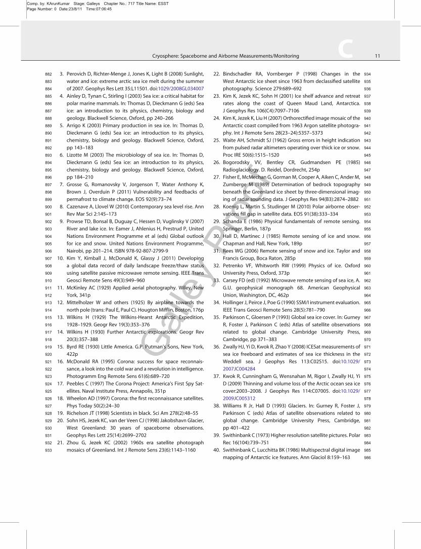
Cryosphere: Spaceborne and Airborne Measurements/Monitoring. Figure 3
European Space Agency MERIS image of Peterman Glacier, Greenland (left). The multispectral image was acquired in July,
2008 and before a large part of the floating ice tongue broke free. Argon panchromatic photograph acquired during the
spring of 1962. The clarity of this early view from space is exceptional and provides a valuable gauge for assessing changes
in glacier ice from the 1960s to the present
0
500
1000
1500
2000
250068.6 68.7 68.8 68.9 69 69.1
Latitude
Dep
th (
m)
69.2 69.3 69.4
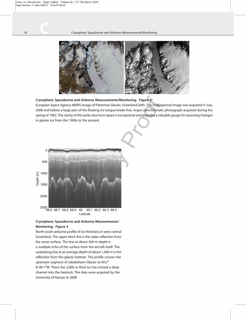
Cryosphere: Spaceborne and Airborne Measurements/
Monitoring. Figure 4
North south airborne profile of ice thickness in west central
Greenland. The upper black line is the radar reflection from
the snow surface. The line at about 500 m depth is
a multiple echo of the surface from the aircraft itself. The
undulating line at an average depth of about 1,400m is the
reflection from the glacier bottom. The profile crosses the
upstream segment of Jakobshavn Glacier at 69.2o
N 48.1oW. There the 2,000 m thick ice has incised a deep
channel into the bedrock. The data were acquired by the
University of Kansas in 2008
16 C Cryosphere: Spaceborne and Airborne Measurements/Monitoring

Comp. by: KArunKumar Stage: Galleys Chapter No.: 717 Title Name: ESSTPage Number: 0 Date:23/8/11 Time:07:06:50
280
260
240
220
200
180
160
140
120
100
Cryosphere: Spaceborne and Airborne Measurements/Monitoring. Figure 5
19 GHz, horizontally polarized, special sensor microwave imager (SSM/I) brightness temperature data for the Arctic on
February 15, 2004 (left) and August 25, 2004 (right). The brightness temperature scale (far right) is in Kelvin. Differences
between the emissivity of ocean, sea ice, land and ice sheets enable the relatively easy identification of the seasonal retreat
in sea ice cover. Brightness temperature variations across the ice pack are caused by differences in ice type and age as well
as in ice concentration
16.0
Average Monthly Arctic Sea Ice ExtentJanuary 1979 to 2011
15.5
15.0
14.5
13.5
14.0
Ext
ent (
mill
ion
squa
re k
ilom
eter
s)
13.0
12.5
12.01978 1982 1986 1990 1994 1998 2002 2006 2010
Year
Cryosphere: Spaceborne and Airborne Measurements/Monitoring. Figure 6
Winter-time Arctic sea ice extent computed using passive microwave data. The decreasing trend illustrates the reduction
in Arctic sea ice extent. There is a muchmore dramatic decline in ice extent during the summer months (Graph courtesy of
the National Snow and Ice Data Center)
17CCryosphere: Spaceborne and Airborne Measurements/Monitoring

Comp. by: KArunKumar Stage: Galleys Chapter No.: 717 Title Name: ESSTPage Number: 0 Date:23/8/11 Time:07:06:52
Cryosphere: Spaceborne and Airborne Measurements/
Monitoring. Figure 7
Canadian RADARSAT-1 Antarctic Mapping Project
synthetic aperture radar mosaic. The radar is sensitive to
changes in the physical structure of the near surface snow.
Bright coastal returns are scattered from subsurface ice
lenses formed during fall freeze-up. Darker interior tones
occur where snow accumulation is high. Other features
such as ice streams and ice divides are visible (Map
courtesy of K. Jezek. RADARSAT-1 data courtesy of the
Canadian Space Agency)
Velocity2
0.5
0.25
km/y
r m/day
0
1.5
1
0.5
0
Cryosphere: Spaceborne and Airborne Measurements/
Monitoring. Figure 8
Surface velocities on Hubbard Glacier Alaska measured
using Japanese PALSAR L-band interferometric pairs.
Hubbard Glacier is a tidewater glacier and ice from the
advancing snout calves directly into Disenchantment Bay
(lower center). Hubbard Glacier is one of the few in Alaska
that is currently thickening and advancing (Image courtesy
of E. W. Burgess and R. R. Forster, University of Utah)
18 C Cryosphere: Spaceborne and Airborne Measurements/Monitoring

Comp. by: KArunKumar Stage: Galleys Chapter No.: 717 Title Name: ESSTPage Number: 0 Date:23/8/11 Time:07:06:53
70°
210°
60°
50°
−12 −10 −8 −6 −4 −2 0 2 4 6
cm eq. H2O / yr
Cryosphere: Spaceborne and Airborne Measurements/Monitoring. Figure 9
Mass loss from Alaskan Glaciers in cm of water equivalent per year from GRACE (Image courtesy of S. Luthcke, NASA GSFC)
Cryosphere: Spaceborne and Airborne Measurements/
Monitoring. Figure 10
Snow cover extent from NASA’s MODIS. Increasing shades
of gray indicate greater percentages of snow cover within
each pixel. Brown denotes snow-free surface
19CCryosphere: Spaceborne and Airborne Measurements/Monitoring

Comp. by: KArunKumar Stage: Galleys Chapter No.: 717 Title Name: ESSTPage Number: 0 Date:23/8/11 Time:07:06:56
Cryosphere: Spaceborne and Airborne Measurements/
Monitoring. Figure 11
January 2010 NASA MODIS image of ice formed on the St.
Lawrence River. Thin layers of new ice are distorted into
swirls by the surface currents (center left). Thicker ice is held
fast to the southern shore (Image courtesy of MODIS Rapid
Response Team, NASA GSFC)
Cryosphere: Spaceborne and Airborne Measurements/
Monitoring. Figure 12
EO-1 Hyperion satellite data acquired over the north coast
of Alaska (70.5 N 156.5 W) and about 50 km inland from the
coast, which is toward the right on this image. The image is
7.5 km wide (top to bottom). Color composite using
channels 16 23 and 28
20 C Cryosphere: Spaceborne and Airborne Measurements/Monitoring

Comp. by: KArunKumar Stage: Galleys Chapter No.: 717 Title Name: ESSTPage Number: 0 Date:23/8/11 Time:07:06:56
02 03 04 05 06 07
Cryosphere Satellite Missions
08 09 10 11 12 13 14 15 16
PALSAR/ALOS L-band
RA, SAR & Wind Scat/ERS-2 RA2 & ASAR/Envisat C-band
RADARSAT-2 C-band
SAR/RISAT C-band
TerraSAR/Tandem-X X-band
SAR/COSMO-SKYMED X-band
ASCAT & AVHRR/MetOp -1, -2, -3
Seawinds/QuikSCAT Ku-band
ICESAT ICESAT-2
CryoSat-2
GRACE
GOCELEO missions
SMOS
AMSR2/GCOM-W1
VIIRS/NPP NPOESS C1
WindSat
OLS & SSMI/DMSP—AVHRR & AMSU/NOAA
MODIS & AMSR-E/EOS-Aqua
Aster/MODIS/EOS-Terra
COCTS/HY-1A HY-1B
VIRR/FY-1D
SPOT-4/5 & Landsat
In Orbit
Solid Colour = R & D mission; Hatched = operational mission
Approved Planned/Pending approval
MODI & MERSI/FY-3A
HY-1C
HY-2A HY-2B
PCW 1 & 2Arctica-M 1 & 2
Courtesy: M. Drinkwater
HEO missions
GMES S-3A, B
GRACE-C
Ku-Scat & MSMR/OCEANSAT-2
IPY
RADARSAT-ConstellationRADARSAT-1 C-band
HY-3 C-, X-band
GMES S-1A, B
Cryosphere: Spaceborne and Airborne Measurements/Monitoring. Figure 13
Current, approved and planned satellites for studying and monitoring the Cryosphere (Figure courtesy of Mark
Drinkwater, European Space Agency)
21CCryosphere: Spaceborne and Airborne Measurements/Monitoring

Comp. by: KArunKumar Stage: Galleys Chapter No.: 717 Title Name: ESSTPage Number: 0 Date:23/8/11 Time:07:06:59
Cryosphere: Spaceborne and Airborne Measurements/
Monitoring. Figure 14
German Aerospace Center TerraSAR-X observations of the
Nimrod Glacier (inset map of Antarctica). Ice floes around
a central nunatak and down toward the Ross Ice Shelf.
Crevasses appear in conjunction with the interruption of
flow by the nunatak. Cooperative use of Canadian,
German, European Space Agency, Italian, and Japanese
synthetic aperture radar (SAR) satellites along with ground
segment and data processing capabilities provided by the
United States yielded a rich and diverse SAR data set that
will be a lasting legacy of the IPY (TerraSAR-X data courtesy
of D. Floricioiu, German Aerospace Center. Inset coastline
derived from RADARSAT-1 Antarctic Mapping Project map)
22 C Cryosphere: Spaceborne and Airborne Measurements/Monitoring

Comp. by: KArunKumar Stage: Galleys Chapter No.: 717 Title Name: ESSTPage Number: 0 Date:23/8/11 Time:07:06:59
Author Query Form
Encyclopedia of Sustainability Science and Technology
Chapter No: 717
___________________________________________________________________________
Query Refs. Details Required Author’s response
AU1 Kindly check and confirm affiliation for authorKenneth C. Jezek.
AU2 Kindly provide index terms.
AU3 Kindly confirm if “475 +- 158 Gt/year” can bechanged to “475 ± 158 Gt/year” in the sentence“Using surface mass balance…”