1 Introduction

Department of Pesticide Regulation Environmental Monitoring Branch

1001 I Street Sacramento, California 95812

Methodology for Evaluating Pesticides for Surface Water Protection: PREM Version 5 Updates

Yuzhou Luo, Ph.D.

May 16, 2017

The Surface Water Protection Program (SWPP) of California Department of Pesticide Regulation (CDPR) is developing a more consistent and transparent method for evaluating registration packages. The first version of the Pesticide Registration Evaluation Model (PREM) was released in 2012 (Luo and Deng, 2012a, b). SWPP keeps improving the model by updating modeling approaches and introducing new simulation capabilities. This report summarizes the model development, improvement, and integration after 2012 (Table 1). Some of the model functions, e.g., the urban pesticide uses (Luo, 2014a) and the identification of exposure potentials to estuarine/marine species (Xie and Luo, 2016), have been presented previously. This report will mainly describe their computational integration with PREM. In this report, “previous version” and “updated model” will be used, respectively, in the description of the previous PREM (version 3) and the newly improved PREM (version 5).

This technical report will mainly present model development, assumptions, and computer implementations for SWPP registration evaluation. Other components in the evaluation process, such as input data preparation, additional data request, modeling results interpretation, professional judgment, and final reporting with registration recommendation, will be provided in the model user’s manual.

Modeling approach for evaluating pesticide degradates and the updated decision-making process will be introduced first. Unlike other model development such as the evaluation methodology for urban pesticide uses which does not affect the overall modeling process, degradate evaluation is implemented by modification and integration on all modeling components of PREM, and significantly changes the decision-making process. Subsequent sections will provide details in the model development and improvement, organized by the five evaluation variables (soil-runoff potential, aquatic persistence, aquatic toxicity, pesticide use pattern, and risk quotient) as previously defined for registration evaluation (Luo and Deng, 2012a, b).

Table 1. Overview of model updates

Modeling components

Previous version (version 3) Updated model in this report (version 5)

Stage 1 Evaluation variables for soil runoff Two additional functions are included: (initial potential, aquatic persistence, and identification of exposure potentials screening) aquatic toxicity are defined in this

stage. to estuarine/marine species (Xie and Luo, 2016)

initial screening of pesticide degradates (Luo et al., 2016)

Stage 2 (refined modeling):

Always require the stage-2 evaluation for aquatic or rice pesticides regardless of the stage-1 results.

Outdoor low- Based on aquatic persistence: Similar to the previous approach, but will risk use High/intermediate persistence: flag the pesticide active ingredient (AI) patterns conditional support

Low persistence: support and flag

regardless of aquatic persistence.

Aquatic Assumed with high risk quotient Based its target concentration or applications application rate, the product will be

evaluated based on VVWM-predicted risk quotients in a template water body.

Rice Based on pesticide concentrations Newly developed evaluation pesticides in a rice paddy at the end of the

water-holding period: USEPA Tier-1 rice model Dissipation of the pesticide AI

methodology for rice pesticide uses based on PFAM.

Urban uses Initially with PRZM modeling scenario for California impervious surfaces, and evaluation methodology for urban pesticide uses (Luo, 2014a) was incorporated in 2014.

Evaluation methodology for urban pesticide uses and new developments.

Agricultural Based on aquatic persistence Simulation engines are updated to the uses (with and PRZM-predicted risk latest versions recently released by high-risk use quotients. USEPA (i.e., PRZM5 and VVWM). patterns) EXAMS simulation will be

conducted if the above evaluation shows high/intermediate persistence and high risk quotient.

Evaluate based on VVWM-predicted risk quotients in a receiving water body.

Additional high-risk use patterns are modeled for agricultural uses.

Seed treatment is explicitly modeled. Pesticide degradates

Not considered Evaluation methodology for pesticide degradates (Luo et al., 2016) and its integration to PREM.

2

2 Evaluation for pesticide degradates

Notes: USEPA models: PRZM = Pesticide Root-Zone Model, EXAMS = Exposure Analysis

Modeling System, VVWM = Variable Volume Water Model, PFAM= Pesticides in Flooded Application Model (USEPA, 2015)

SWPP is developing more representative modeling scenarios for receiving water body in California field conditions, in terms of dimensions, physical characteristics, hydrological conditions, and surrounding watershed descriptions (Xie, 2014). Once the development is completed, the scenario will be applied to all stage-2 evaluations for high-risk use patterns. Meanwhile, USEPA standard pond scenario is used.

Degradate evaluation in PREM is developed for one or multiple degradates of the pesticide AI. To simplify the modeling process and data request, major degradates are modeled as direct degradation products of the pesticide AI. The integration of the degradate evaluation to the PREM modeling framework is introduced here, while the theoretical considerations have been documented separately (Luo et al., 2016). Three procedures are involved in the degradate evaluation:

(1) Identification of the degradates for which toxicity data are needed for further evaluation. If none of the degradates need further evaluation, stop degradate evaluation and make recommendations based on the results for the pesticide AI only.

(2) Preparation of toxicity data for the degradates identified in (1), and identify the degradates for which model-based evaluation is needed. If none of the degradates need model-based evaluation, stop degradate evaluation and make recommendations based on the results for the pesticide AI only.

(3) Model-based evaluation for the pesticide AI and degradates identified in (2).

The procedures (1) and (2) implement the proposed initial screening of degradates (Luo et al., 2016), which generates a list of degradates to be modeled, and (3) is conducted by the stage-2 evaluation in PREM together with the pesticide AI. Solely based on data of the pesticide AI, the procedure (1) will determine if there are candidate degradates for additional evaluation. If so, a list of the candidate degradates and associated criteria for model-based evaluation will be reported as model outputs. In the procedure (2), the reviewer will prepare toxicity data for the procedure (1)-identified degradates, and identify the degradates for model-based evaluation in (3). While the procedures (1) and (3) are fully integrated in the model, data analysis and data request (if applicable) of degradate toxicity will be manually handled by a reviewer as a part of input data preparation.

For consistent computational implementation for the pesticide AI only and AI-degradates combined evaluations, a variable, nDeg, is introduced as the total number of degradates to be modeled. Two sets of model simulations may be required:

The first round of evaluation, with nDeg initially set as zero (nDeg=0). The model will perform registration evaluation for the pesticide AI and the procedure (1) for degradate initial screening.

3

The second round of evaluation, if there is at least one degradate (nDeg>0) requiring model-based evaluation according to the procedure (2) results. Evaluation will be conducted for the pesticide AI and the identified degradates.

3 Decision-making process

Decision-making process generates modeling results including registration recommendations (support, conditionally support, or not support), data requests (analytical methods and/or degradate toxicity), AI flagging for future evaluation, and watch-list of pesticides for surface water monitoring. With the integration of the degradate evaluation, two components are developed for the decision-making process: model-based evaluation and modeling control.

3.1 Model-based evaluation

Model-based evaluation is developed to quantify the variables (soil-runoff potential, aquatic persistence, aquatic toxicity, use pattern, and risk quotient) and make registration recommendations. The flowchart for model-based evaluation (Figure 1) is similar to the previous version (Luo and Deng, 2012a), but updated for risk quotient calculation based on pesticide concentrations in a receiving water body. In addition, the stage-2 evaluation is always required for aquatic and rice pesticides regardless of the stage-1 results. Compared to the previous version, the updated model will calculate risk quotients for aquatic and rice pesticides even when the AI is not highly toxic. Unlike terrestrial applications, aquatic and rice pesticides are directly applied to the water body where the risk quotient is calculated. Therefore, it’s scientifically sound to characterize their potential risks to aquatic ecosystems based on application information, i.e., the stage-2 evaluation.

Model-based evaluation can be applied to the pesticide AI only (nDeg=0, where nDeg is the number of pesticide degradates to be modeled), or the pesticide AI and degradates (nDeg>0) (Table 2). For the evaluation of the pesticide AI only, the pesticide AI will be evaluated by stage I (initial screening, with evaluation variables of soil-runoff potential, aquatic persistence, and aquatic toxicity), and followed by stage II (refined modeling, with use pattern and risk quotient), if applicable. For evaluations on the pesticide AI and selected degradates, only risk quotient is calculated (other evaluation variables have been considered during the initial screening of pesticide degradates). In this case, both individual risk quotients (for each chemical) and total risk quotient (TRQ, combined for the pesticide AI and all modeled degradates) will be reported.

4

Figure 1. Model-based evaluation process for the pesticide AI and degradates (descriptive classifications: L=low, M=intermediate, H=high, VH=very high. The recommendation ID’s are explained in Table 2). T=true and F=false.

5

Table 2. Model-based registration recommendations

ID (Figure 1)

Criteria Registration recommendation

Additional actions

10 Low-to-intermediate toxicity Support 20 Low-to-intermediate soil-runoff

potential Support

30 Low risk quotient (TRQ≤0.1) Support 40 Low-risk use pattern and low aquatic

persistence (but high toxicity or high soil-runoff potential)

Support Flag the AI for future evaluation

50 Intermediate risk quotient (0.1<TRQ≤0.5)

Conditionally support

Request analytical method for the AI and degradates with RQ(D)>0.1

60 Low-risk use pattern and high/intermediate aquatic persistence (but high toxicity or high soil-runoff potential)

Conditionally support

Request analytical method for the AI, and flag the AI for future evaluation

70 High risk quotient (TRQ>0.5) Not support Notes: Recommendation ID’s are shown in Figure 1. TRQ = total risk quotient of the pesticide AI and degradates to be modeled, RQ(P) = RQ for the pesticide AI, and RQ(D) = RQ for a degradate.

AI flagging is applied to some of the pesticide AI’s for which the currently product under evaluation is supported or conditionally supported for registration. It’s designed to capture potential, significant changes in pesticide use patterns (e.g., from low- to high-risk; or change between aquatic and terrestrial) for future products with the same AI. Additional discussions on AI flagging are provided as follows:

1. In the previous version, an AI will be flagged if the product is only labelled for low-risk use pattern AND low aquatic persistence. In this version, AI’s will be flagged for low-risk use patterns regardless of their aquatic persistence (recommendation ID’s of 40 and 60, Table 2). The flag is internally used for CDPR to ensure that, even registration is supported for the current product, future submissions of products with the same AI’s will be routed to and evaluated by SWPP in case their new labels are associated with high-risk use patterns.

2. Not shown in the flowchart, there is another situation of AI flagging during degradate evaluation: the AI is associated with quick degradation but the degradation pathways do not match the proposed use patterns (Luo et al., 2016). For example, quick degradation in aerobic soil metabolism is observed for the AI, but the product is proposed for aquatic applications. In this case, degradates from aerobic soil metabolism are not considered for degradate evaluation, but the AI will be flagged for future labels with terrestrial applications.

6

Evaluations in Figure 1 are conducted separately for water column and bed sediment, and the worse condition in the model-based recommendations are reported for the pesticide product under evaluation. For example, if the result of water column evaluation supports registration but that for bed sediment does not support registration, the model will not recommend the product for registration.

3.2 Modeling control

Evaluation for the pesticide AI and initial screening of pesticide degradates are considered as independent, parallel processes (Luo et al., 2016); therefore, modeling control is needed to manage the two processes. Model-based evaluation may have to run twice: for the pesticide AI; and for the pesticide AI and degradates (Figure 2). The overall modeling procedure can be described as follows:

(1) First, the model will conduct evaluations on the pesticide AI only (by setting nDeg=0), and initial screening of degradates.

(2) If the evaluation results for the pesticide AI suggest denial of product registration, the model will stop here. Both the model-based recommendation (in this case, denial) and results of the initial screening of degradates will be presented in the evaluation report.

(3) Otherwise, if the evaluation results for the pesticide AI support or conditionally support registration, reviewers will be asked to prepare toxicity data for the identified degradates and finalize the list of degradates to be modeled. This will be the same procedure documented in Section 2, procedure (2).

(4) If none of the pesticide degradates need model-based evaluation, the model will stop here. Model-based recommendations for registration actions will be based on the evaluation results for the pesticide AI only.

(5) If there are some degradates need model-based evaluation, model-based evaluation will be conducted again with degradate evaluation enabled (by setting a positive nDeg according to the number of degradate s to be modeled). Model-based recommendations for registration actions will be based on the evaluation results for the pesticide AI and degradates.

The proposed modeling processes are demonstrated in the Appendix with a hypothetical chemical and its degradates.

7

Figure 2. PREM modeling control for model-based evaluation and initial screening of pesticide degradates. nDeg = the number of pesticide degradates to be modeled. nDeg=0 indicates an evaluation for the pesticide AI only. T=true and F=false.

4 Variables for registration evaluation

The following paragraphs explain the derivation of the evaluation variables from model input parameters, including toxicity data, molecular weight, water solubility, KOC, vapor pressure, dissipation/degradation half-lives, and formation fractions. The same set of input values are used for the stage-1 and stage-2 variables.

4.1 Soil-runoff potential

There are no changes on the descriptive classification for soil-runoff potential since the previous development (Luo and Deng, 2012a). The same methodology was also used in the identification of pesticide exposure potential to estuarine/marine species (Xie and Luo, 2016).

In summary, if the pesticide product under evaluation is proposed to be applied to aquatic sites, rice paddies, or impervious surfaces, its runoff potential is set to be “High”. Otherwise, the

8

criteria in Table 3 are used to classify a “High” runoff potential for applications to soil and canopy.

Table 3. Classification criteria for “High” runoff potential from soils (Luo and Deng, 2012a) Criteria

Dissolved phase (SOL ≥ 1 and FD > 20 and KOC < 1×105) or (SOL ≥ 10 and KOC ≤ 2000)

Adsorbed phase (FD ≥ 15 and KOC ≥ 4×104) or (FD ≥ 40 and KOC ≥ 1000) or (SOL ≤ 0.5 and FD ≥ 40 and KOC ≥ 500)

Notes: SOL (ppm) = water solubility, FD (day) = field dissipation half-life, KOC (L/kg[OC]) = organic carbon-normalized soil adsorption coefficient.

4.2 Aquatic persistence

In the updated PREM, recommendations for low-risk use patterns are determined based on aquatic persistence, where high or intermediate persistence leads to conditional supported registration and low persistence leads to supported registration (Figure 1). There are no changes on the descriptive classification for aquatic persistence as presented in the previous development (Luo and Deng, 2012a) (Table 4). The same classification was also used in the identification of pesticide exposure potential to estuarine/marine species (Xie and Luo, 2016).

Table 4. Classification criteria for aquatic persistence (Luo and Deng, 2012a)

Criteria Persistence rating HL ≥ 100 High (H) 30 ≤ HL < 100 Intermediate (M) HL < 30 Low (L) Notes: HL (day) is the representative half-life, which is determined separately for water and sediment evaluations. In water, HL=min(hydrolysis half-life, aquatic metabolism half-life); in sediment, HL = anaerobic aquatic metabolism half-life.

4.3 Acute aquatic toxicity

In the previous version PREM, acute aquatic toxicity (TOX) was calculated as the minimal value of all reported acute EC50 or LC50 values, including those for freshwater, estuarine, and marine species (fish and/or invertebrates). This is improved by specifying required toxicity tests according to the product’s exposure potential to estuarine/marine species (Table 5).

9

Table 5. Required toxicity tests for registration evaluation

KOC of the Exposure potential of Required toxicity tests pesticide AI the pesticide product to

estuarine/marine species Water column Bed sediment

KOC≤1000 High Freshwater and estuarine/marine species

N/R

Low Freshwater species only N/R KOC>1000 High Freshwater and

estuarine/marine species Freshwater and estuarine/marine species

Low Freshwater species only Freshwater species only

Notes: (1) N/R: not required. Generally, sediment evaluation for an AI with KOC≤1000 is not

required. With considerations of pesticide degradates, however, sediment evaluation may be triggered by some of its degradates with KOC>1000.

(2) Exposure potential to estuarine/marine species. High: require toxicity tests to both freshwater and estuarine/marine species; Low: only require tests to freshwater species

(3) Toxicity tests in water column include those for freshwater invertebrates (OPPTS Guidelines 850.1010), mysid (850.1035), and freshwater/marine fish (850.1075). Sediment toxicity can be derived from tests for freshwater invertebrates (850.1735), and estuarine/marine invertebrate (850.1740) (USEPA, 2014a).

(4) If required toxicity tests for sediment-dwelling species are not submitted or accepted, SWPP will run preliminary evaluation with water toxicity data as a surrogate. Based on the results, SWPP will determine if additional data are needed.

The identification of high exposure potential to estuarine/marine species were documented in Xie and Luo (2016), according to the evaluation variables of pesticide use pattern, soil-runoff potential, and aquatic persistence. In the updated PREM, this process is incorporated in the stage-1 evaluation. Based on KOC and exposure potentials to estuarine/marine species, the model will inform reviewers of the required toxicity tests (Table 5), and ask reviewers to verify/update toxicity values as model inputs.

Sediment toxicity is used in the evaluation of pesticide in bed sediment, which is only required if the pesticide AI or degradates to be modeled with KOC>1000 (Luo and Deng, 2012a). Input data of sediment toxicity could be expressed in one of the three formats: pore-water concentration (µg/L), sediment mass based (µg/kg[dry sediment]), or organic carbon (OC) normalized (µg/g[OC]). VVWM only reports pesticide level in bed sediment in the form of aqueous concentration in pore water. For the calculation of risk quotients, therefore, sediment toxicity will be converted to equivalent value as pore-water concentration with the assumption of instantaneous equilibrium. For example,

For toxicity value in µg/kg[dry sediment], the equivalent value as pore-water concentration TOX(µg/L) = [provided value]/fOC/KOC.

10

For toxicity value in µg/g[OC], the equivalent value as pore-water concentration TOX(µg/L) = [provided value]*1000/KOC.

where fOC is the organic carbon content in the bed sediment. If no experimental data are available, fOC is set to 4% according to USEPA standard pond scenario. The converted values of sediment toxicity will be also reported in the modeling results. If sediment toxicity data are missing, the model will remind a user to check the input data, or set the same value of water toxicity for sediment toxicity after user’s confirmation.

Once TOX values for bulk water and pore water are determined, the variables for aquatic toxicity, in water and in sediment, are defined by following the description classifications by USEPA (Zucker, 1985).

4.4 Pesticide use patterns

Only pesticide products with high-risk use patterns will be required for refined modeling processes (Luo and Deng, 2012b). In the previous version, high-risk use patterns were determined based on expert opinions and statewide data analysis on irrigation methods, and planted and treated acreage. During the identification of high exposure potential to estuarine/marine species (Xie and Luo, 2016), additional high-risk use patterns were identified based on similar data analysis but for California coastal areas (Table 6).

For seed treatment, its risk potential is also determined by the corresponding crop type. If it’s associated with any of the crops in Table 6, it will be considered as high-risk use pattern and subject to additional evaluation.

Application efficiency and spray drift are considered in the updated model according to pesticide use patterns. Default input values are listed in Table 7. In addition, the model also provides options for user-specified values to reflect use restrictions and associated modeling results (such as AgDRIFT and AGDISP). For urban outdoor uses, usually a small portion of an urban watershed is actually treated. Therefore, its application efficiency is set as 100% and drift fraction as zero. In addition, the incidental application and deposition to non-target urban surfaces are considered by USEPA and SWPP with a overspray factor (USEPA, 2007; Luo, 2014a).

11

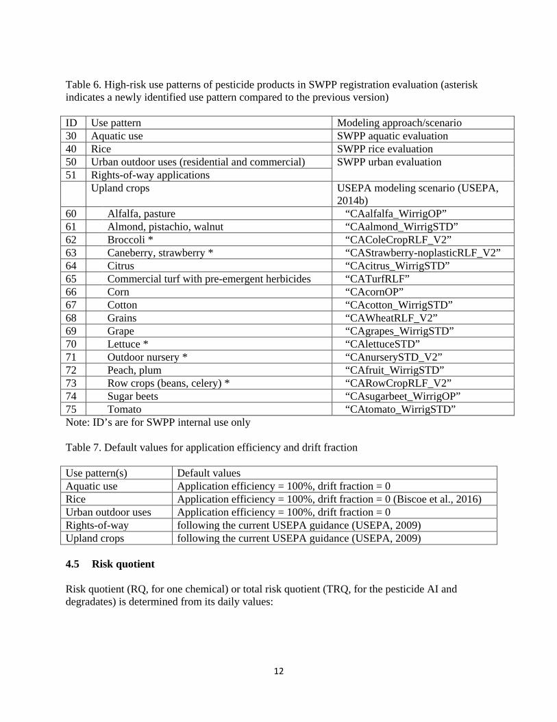
Table 6. High-risk use patterns of pesticide products in SWPP registration evaluation (asterisk indicates a newly identified use pattern compared to the previous version)

ID Use pattern Modeling approach/scenario 30 Aquatic use SWPP aquatic evaluation 40 Rice SWPP rice evaluation 50 Urban outdoor uses (residential and commercial) SWPP urban evaluation 51 Rights-of-way applications

Upland crops USEPA modeling scenario (USEPA, 2014b)

60 Alfalfa, pasture “CAalfalfa_WirrigOP” 61 Almond, pistachio, walnut “CAalmond_WirrigSTD” 62 Broccoli * “CAColeCropRLF_V2” 63 Caneberry, strawberry * “CAStrawberry-noplasticRLF_V2” 64 Citrus “CAcitrus_WirrigSTD” 65 Commercial turf with pre-emergent herbicides “CATurfRLF” 66 Corn “CAcornOP” 67 Cotton “CAcotton_WirrigSTD” 68 Grains “CAWheatRLF_V2” 69 Grape “CAgrapes_WirrigSTD” 70 Lettuce * “CAlettuceSTD” 71 Outdoor nursery * “CAnurserySTD_V2” 72 Peach, plum “CAfruit_WirrigSTD” 73 Row crops (beans, celery) * “CARowCropRLF_V2” 74 Sugar beets “CAsugarbeet_WirrigOP” 75 Tomato “CAtomato_WirrigSTD” Note: ID’s are for SWPP internal use only

Table 7. Default values for application efficiency and drift fraction

Use pattern(s) Default values Aquatic use Application efficiency = 100%, drift fraction = 0 Rice Application efficiency = 100%, drift fraction = 0 (Biscoe et al., 2016) Urban outdoor uses Application efficiency = 100%, drift fraction = 0 Rights-of-way following the current USEPA guidance (USEPA, 2009) Upland crops following the current USEPA guidance (USEPA, 2009)

4.5 Risk quotient

Risk quotient (RQ, for one chemical) or total risk quotient (TRQ, for the pesticide AI and degradates) is determined from its daily values:

12

RQi (t) = EEC(t) / TOX , for a chemical i (1) TRQ(t) = ∑RQi (t)

i

where i is a running index for chemicals to be modeled (i≥1), EEC(t) is the time series of daily average concentrations of the pesticide predicted by VVWM during the 30-year simulation period of 1961-1990, and TOX is the toxicity value of the corresponding chemical as modeling input determined in Section 4.3. Risk quotients are calculated in both water column (with concentration and toxicity values in water column) and bed sediment (with concentration and toxicity values in pore water). TRQ is calculated as the 1-in-10-year TRQ(t), i.e., the 90th

percentile of annual maximum TRQ(t) for the 30 years. The evaluation variable of risk quotient is descriptively classified as: high risk quotient for TRQ>0.5, intermediate risk quotient for 0.1<TRQ≤0.5, and low risk quotient for TRQ≤0.1 (Table 2). Similarly, RQ for a chemical is calculated from the corresponding RQ(t) as 1-in-10-year maximum value, and used to determine if analytical methods are to be requested for the chemical (Table 2). The following subsections describe the prediction of daily concentrations and risk quotients in a template receiving water body.

4.5.1 Aquatic pesticide uses

This evaluation methodology is developed for pesticides directly applied to a water body other than rice paddy. The aquatic evaluation is developed to [1] generate input files for VVWM based on the target concentration and application dates of pesticides, [2] manage VVWM simulations for multiple chemicals (the pesticide AI and selected degradates), if applicable, and [3] to calculate risk quotients for the pesticide AI and degradates.

For aquatic pesticide products, the use directions may be presented as application rates for various water depths, or as the target or maximum concentration to be established in water (Ctarget, µg/L). Note that the target concentration is not the dissolved concentration of the pesticide in the water column after application, but most likely estimated based on the application rate and corresponding water depth:

Ct arg et = 100 ⋅ LABEL / d1 (2)

where LABEL (kg/ha) is the application rate at the specific water depth d1 (m), and 100 is a constant for unit conversion. If either application rate (and associated water depth) or target concentration is available, VVWM will be used for pesticide fate simulation in the treated water body. Otherwise, if neither the application rate nor target concentration can be determined from the product label, risk quotients will be conservatively assumed to be “High”.

For VVWM simulations, USEPA standard pond scenario is used as the default water body. A user-defined water body is also allowed if the desired water depth for aquatic application in the product label is significantly different to the standard pond scenario (i.e., 2m). In this case, the standard pond scenario is modified with the specified depth, while keeping other parameters invariant. The model simulation requires weather data. The USEPA weather file “w23232.dvf” (Sacramento, CA), one of the standard meteorological data for exposure assessment models, is

13

used for the evaluation of aquatic pesticide uses. Please note that the USEPA standard pond scenario assumes constant volume and no flowthrough (Young, 2016). Therefore, VVWM results may not be very sensitive to weather data.

VVWM requires input data in the format of PRZM output. For direct application to a water body, an artificial PRZM output file is developed by converting the target concentration to application rate (kg/ha), then to the edge-of-field runoff flux of dissolved pesticide (in the PRZM terminology: RFLX, g[AI]/cm2/day):

− Ctarget ⋅ v1RFLX = 1×10 11 ⋅ (3) AFIELD

where AFIELD (ha) is the field size, v1 (m3) is the water volume, and 1e-11 is a constant for unit conversion. For USEPA standard pond scenario (i.e., AFIELD=10 ha and v1=20,000 m3), RELX = (2e-8)×C.

In VVWM, the flux (RFLX) is further converted to the mass of the aquatic pesticide application, Mrunoff (kg/day, mass of pesticide entering water body via runoff) (Young, 2016). In this process, AFIELD is cancelled and won’t affect further simulations:

5 −6M runoff = 1×10 ⋅ RFLX ⋅ AFIELD = 1×10 ⋅ Ctarget ⋅ v1 (4)

4.5.2 Rice pesticide uses

This evaluation methodology is developed for rice pesticides, and also can be used for other similar crop types such as cranberry and taro. Compared to other use patterns, additional input data required for rice pesticides include water-holding period and physical characterizations of the rice paddy. PFAM (Pesticides in Flooded Application Model) is used as the simulation engine in the evaluation of rice pesticides.

PFAM input parameters for environmental description, crop growth and water management are taken from USEPA modeling scenarios for ecological risk assessments of rice pesticides in California (White et al., 2016). Simulations for spray drift and downstream waterbody are not suggested by USEPA for ecological risk assessments, only applied in drinking water assessments. The specific USEPA scenario used in the evaluation is the “California Winter Flood”, modified by adding events of water release and re-flooding according to pesticide applications and water-holding periods specified by the user. Finally, the evaluation assumes no “turnover” in the paddy when the holding period is in place.

For the 30-year simulation period of 1961–1990, daily average concentrations of pesticide in paddy water and sediment (as pore-water concentration) on the days of intended water release are used to calculate the 1-in-10-year EEC. Intended water release includes drains after water-holding period and those prior to harvest. This approach for risk characterization is different to that of USEPA, in which concentrations on all simulation days, including those immediately after applications, are considered for risk characterization. The use of concentrations at the end

14

House

Garden

Sidewalk

Lawn

Driv

eway

10ft

of water-holding period reflects the mitigation effects that reduce pesticide runoff to adjacent waterbodies.

4.5.3 Urban pesticide uses

This evaluation methodology is developed for pesticide outdoor uses in urban environment with intended or unintended applications to impervious surfaces, including residential or commercial/industrial outdoor uses, and right-of-way applications. Development and integration of the urban evaluation was described previously (Luo, 2014a), and has been integrated in the previous version of PREM (Luo and Singhasemanon, 2014). The following new developments are incorporated in this version.

(1) The simulation engines are updated from PRZM3/EXAMS to PRZM5/VVWM. (2) Insecticide application extent is considered for residential uses. In the previous urban

scenarios used by USEPA and SWPP, it’s assumed that all households in the 10-ha template urban watershed will use the pesticide for outdoor pest control. In the updated model, the label rate is adjusted by the fraction of households treated with residential outdoor pesticide products (75.9%). This fraction is based on survey results (Winchell and Cyr, 2013) submitted by Pyrethroids Working Group (PWG), and reviewed by SWPP (Luo, 2014b).

(3) Hydrologic connectivity of paved areas is considered for residential uses of pesticides. The updated model assumes that only the impervious surfaces (paved areas and walls) in the front yard of a house could result in runoff into storm drains (Figure 3). Other impervious surfaces will drain through adjacent pervious surfaces. To simplify the simulation while remain conservative estimations, pesticide applications to this portion of impervious surfaces are simulated with modeling scenarios for pervious surfaces without dry-weather runoff, i.e., the surface #1 in the urban evaluation.

(a) Modeled components of residential landscape

(b) Impervious surfaces in the front of the house (delineated as 10ft from the f ront wall) will r esult in runoff into storm drains, while other impervious surfaces will drain through pervious surfaces

Figure 3. Conceptual model for evaluating pesticide uses in residential areas (not to scale)

15

(4) “Right-of-way” application is separated from urban outdoor uses in the list of high-risk use patterns (Table 6). There is no change on the modeling approach for right-of-way applications as described in the technical report of the urban evaluation (Luo, 2014a).

(5) Coordination of physiochemical properties which are originally developed for soils, but used in the urban evaluation.

a. Pesticide degradation on impervious surfaces is simulated with the value of soil photolysis half-life (SPHOT). In addition, if the effective dissipation half-life of pesticide on impervious surfaces is provided by registrants and accepted by CDPR, the value could be used in urban evaluation by replacing SPHOT.

b. Degradate formation on impervious surfaces is simulated with the value of DKS (formation fraction in the soils). In addition, if the corresponding value for the transport process on impervious surfaces is provided by registrants and accepted by CDPR, it could be used in the urban evaluation by assigning to DKS.

In the urban evaluation, typical application methods to be modeled include lawn broadcast, applications to paved areas, perimeter treatment, wall treatment, and crack and crevice treatment. Pesticide uses which are not directly applied to impervious surfaces, by either intended or unintended, are generally not considered as high-risk use patterns. Examples of these application methods include bait stations, vapor dispersion, spot treatment of foaming products to wooden structures, and treatments to fence, garden, bushes, and trees. These applications are usually not associated with a label rate in the form of AI mass per unit area, thus cannot be directly modeled in the urban evaluation. However, if significant amount of pesticide could be received by the underneath or nearby paved areas via deposition or washoff processes from the treated areas, modeling can be conducted based on the conservative estimation of release rates on the impervious surfaces. The urban model provides options of user-defined treated areas (by fractional coverages) for modeling flexibility to handle those special cases of urban outdoor pesticide uses.

4.5.4 Agricultural pesticide uses

Agricultural pesticide products with high-risk use patterns will be evaluated based on PRZM5 and VVWM models. PRZM modeling scenarios used in the PREM simulations are listed in Table 6, and USEPA standard pond scenario is used as default in VVWM simulations.

Acknowledgements

The author would like to acknowledge Nan Singhasemanon, Yina Xie, Xin Deng, Kean S. Goh, David Duncan, and Ann Prichard for discussions and reviews.

16

References

Biscoe, M.L., Fry, M., Hetrick, J., Orrick, G., Peck, C., Ruhman, M., Shelby, A., Thurman, N., Villanueva, P., White, K., Young, D. (2016). PFAM Version 2.0: Guidance for Selecting Input Parameters for the Pesticide in Flooded Applications Model (PFAM), Including Specific Instructions for Modeling Pesticide Concentrations in Rice Growing Areas (https://www.epa.gov/sites/production/files/2016-10/documents/pfam-input-parameter­guidance.pdf). U.S. Environmental Protection Agency, Washington, DC.

Luo, Y., Deng, X. (2012a). Methodology for evaluating pesticides for surface water protection, I: initial screening (http://cdpr.ca.gov/docs/emon/surfwtr/sw_models.htm). California Department of Pesticide Regulation. Sacramento, CA.

Luo, Y., Deng, X. (2012b). Methodology for evaluating pesticides for surface water protection, II: refined modeling (http://cdpr.ca.gov/docs/emon/surfwtr/sw_models.htm). California Department of Pesticide Regulation. Sacramento, CA.

Luo, Y. (2014a). Methodology for evaluating pesticides for surface water protection: Urban pesticide uses (http://cdpr.ca.gov/docs/emon/surfwtr/sw_models.htm). California Department of Pesticide Regulation, Sacramento, CA.

Luo, Y. (2014b). SWPP Review: PWG survey for outdoor insecticide use (CDPR internal webpage: http://em/localdocs/pubs/rr_revs/rr1451.pdf).

Luo, Y., Singhasemanon, N. (2014). User manual for Pesticide Registration Evaluation Model (PREM) (http://cdpr.ca.gov/docs/emon/surfwtr/sw_models.htm). California Department of Pesticide Regulation, Sacramento, CA.

Luo, Y., Singhasemanon, N., Deng, X. (2016). Methodology for Evaluating Pesticides for Surface Water Protection: Pesticide degradates (http://cdpr.ca.gov/docs/emon/surfwtr/sw_models.htm). California Department of Pesticide Regulation (CDPR), Sacramento, CA.

USEPA (2007). Risks of Carbaryl Use to the Federally-Listed California Red Legged Frog (Rana aurora draytonii) (https://www.epa.gov/endangered-species). U.S. Environmental Protection Agency, Office of Pesticide Programs, Washington, DC.

USEPA (2009). Guidance for selecting input parameters in modeling the environmental fate and transport of pesticides, version 2.1 (https://www.epa.gov/pesticide-science-and-assessing­pesticide-risks/guidance-selecting-input-parameters-modeling). U.S. Environmental Protection Agency, Office of Pesticide Programs, Washington, DC.

USEPA (2014a). OCSPP harmonized test guidelines, series 850 ecological effects test guidelines (http://www.epa.gov/ocspp/pubs/frs/publications/OPPTS_Harmonized/850_Ecological_E ffects_Test_Guidelines/Drafts/). U.S. Environmental Protection Agency, Office of Chemical Safety and Pollution Prevention, Washington, DC.

USEPA (2014b). USEPA Tier 2 crop scenarios for PRZM/EXAMS Shell and Surface Water Concentration Calculator (http://www.epa.gov/oppefed1/models/water/index.htm). U.S. Environmental Protection Agency, Office of Pesticide Programs. Washington, DC.

USEPA (2015). Water exposure models used by the Office of Pesticide Programs (http://www.epa.gov/oppefed1/models/water/). U.S. Environmental Protection Agency, Office of Pesticide Programs. Washington, DC.

White, K., Biscoe, M., Fry, M., Hetrick, J., Orrick, G., Peck, C., Ruhman, M., Shelby, A., Thurman, N., Young, D., Villanueva, P. (2016). Metadata for Pesticides in Flooded

17

Applications Model Scenarios for Simulating Pesticide Applications to Rice Paddies (https://www.epa.gov/pesticide-science-and-assessing-pesticide-risks/models-pesticide­risk-assessment). Environmental Fate and Effects Division, Office of Pesticide Programs, Office of Chemical Safety and Pollution Prevention, U.S. Environmental Protection Agency, Washington, DC.

Winchell, M.F., Cyr, M.J. (2013). Residential Pyrethroid Use Characteristics in Geographically Diverse Regions of the United States. PWG-ERA-02a.

Xie, Y. (2014). Protocol to develop a California-based water quality model for pesticide registration evaluation, DPR study 293 (http://cdpr.ca.gov/docs/emon/pubs/protocol.htm). California Department of Pesticide Regulation.

Xie, Y., Luo, Y. (2016). Methodology for screening pesticide products with high exposure potentials to marine/estuarine organisms (http://cdpr.ca.gov/docs/emon/surfwtr/sw_models.htm). California Department of Pesticide Regulation, Sacaramento, CA.

Young, D.F. (2016). The variable volume water model, Revision A. USEPA/OPP/734S16002, March 2016.

Zucker, E. (1985). Hazard Evaluation Division, Standard Evaluation Procedure: Acute toxicity test for freshwater fish. EPA-540/9/85-006. U.S. Environmental Protection Agency, Office of Pesticide Programs, Washington, DC.

Appendix: Model demonstration

The case study below is presented for the purpose of model demonstration. The demonstrated registration evaluation processes cover most of the PREM modeling capabilities, including urban evaluation, degradate evaluation, and toxicity data preparation according to exposure potential to marine/estuarine species.

It assumes that a registrant submitted the product “Insecticide X” for registration with CDPR, containing 20% of a hypothetical active ingredient “P”. The label proposes surface/broadcast applications on residential areas. SWPP staff selected the modeling scenario of “application on paved areas” to better delineate the potential of the product to impact surface water. Other settings for pesticide application are summarized as: application rate = 0.81 kg[AI]/ha, number of applications per year = 4, and application interval = 30 days.

Two major degradates of P are assumed: D1 and D2, both in soils. Chemical properties, environmental fate data, and toxicity values are prepared by following the guideline for model input data (Luo and Singhasemanon, 2014) (Table 8).

18

Table 8. Model input values for the hypothetical pesticide “P” and its degradates Input parameter P D1 D2 Water solubility (mg/l) 0.2 0.8 1.37 KOC 5800 24500 6356 Hydrolysis half-life (HL) 38 Stable Stable Aerobic soil metabolism HL 80 42 Stable Anaerobic soil metabolism HL 207 42 Stable Aerobic aquatic metabolism HL Stable Stable Stable Anaerobic aquatic metabolism HL Stable Stable Stable Molecular weight 527.87 469.8 469.8 Vapor pressure (torr) 1E-07 NA (set as 1e-15) NA (set as 1e-15) Aqueous photolysis half-life 3.16 Stable Stable Soil photolysis half-life 139 Stable Stable Formation fraction and pathway (for degradate only)

- 0.209 (soil) 0.018 (soil)

Lowest toxicity in water (µg/L), based on acute toxicity test results to estuarine invertebrates

54.2 2.6 5.8

As summarized in Section 3.2 “Modeling control”, the PREM evaluation includes five steps:

Step (1): Evaluation for the pesticide AI and initial screening of degradates

Model outputs are shown in Figure 4. In summary, based on the data for pesticide AI only, modeling results support conditional registration of the product, and request additional investigations on degradates.

In addition, the model also raises some warnings. [1] The product X may be associated with high exposure potentials to marine/estuarine species, so the corresponding toxicity test results should be considered for the model input data of aquatic toxicity. Those tests have been included in the parameter preparation (Table 8). [2] Sediment toxicity test data are not available. As a model option, sediment toxicity (in the form of pore water concentration) is set to the same value of water toxicity. The model reminds the user to check the data availability before finalizing the evaluation.

19

Inputs: e-fate and toxicity data ================================================================= // see Table 8 //

Inputs: use pattern and application rate ================================================================= Urban outdoor | use pattern

High | exposure risk to surface water (high/low) Urban outdoor | modeling scenario

0.81 | the maximum label rate for a single application (kg/ha) Yes | Application extent adjustment for residential insecticide uses 4 | the maximum number of applications per season/year 30 | the minimum application interval (day) 1-1 | date of first application (dd-mm)

Inputs: treated area of each sub-region, in fraction of the urban watershed =================================================================

0.000% | pervious surface, without dry-weather runoff 0.000% | impervious surface, without dry-weather runoff 0.000% | pervious surface, with dry-weather runoff 9.000% | impervious surface, with dry-weather runoff

Outputs: water column (dissolved phase) =================================================================

High | soil-runoff potential (based on SOL, KOC, FD, and use pattern) Intermediate | aquatic persistence (based on half-lives in aquatic system)

Very High | aquatic toxicity 0.39 | risk quotient in the receiving water

Watch | modeling result

Outputs: sediment (adsorbed phase) =================================================================

High | soil-runoff potential (based on SOL, KOC, FD, and use pattern) High | aquatic persistence (based on half-lives in aquatic system)

Very High | aquatic toxicity 0.11 | risk quotient in the receiving water

Watch | modeling result

Overall modeling results (for the pesticide AI only) ================================================================= data/information support conditional registration with data request of analytical method for the AI

Initial screening results for degradates ================================================================= The following degradates may need model-based evaluation: All major degradates, if they are more toxic than the pesticide AI.

Figure 4. PREM5 outputs for the evaluation based on the data for the pesticide AI only.

Step (2): This step is only needed for the denial of product registration, so skipped

Step (3): Preparation of degradate data, see Table 8

Step (4): Determination of degradates to be modeled.

20

Both degradates D1 and D2 are more toxic than the pesticide AI (Table 8), and thus should be modeled (nDeg=2).

Step (5): Model evaluation for the pesticide AI a nd selected degradates

Model outputs are shown in Figure 5. In summary, modeling results support conditional registration of the products and request analytical methods for the pesticide AI.

Inputs: e-fate and toxicity data ================================================================= // see Table 8 //

Inputs: use pattern and application rate ================================================================= Urban outdoor | use pattern

High | exposure risk to surface water (high/low) Urban outdoor | modeling scenario

0.81 | the maximum label rate for a single application (kg/ha) Yes | Application extent adjustment for residential insecticide uses 4 | the maximum number of applications per season/year 30 | the minimum application interval (day) 1-1 | date of first application (dd-mm)

Inputs: treated area of each sub-region, in fraction of the urban watershed =================================================================

0.000% | pervious surface, without dry-weather runoff 0.000% | impervious surface, without dry-weather runoff 0.000% | pervious surface, with dry-weather runoff 9.000% | impervious surface, with dry-weather runoff

Outputs: water column (dissolved phase) =================================================================

High | soil-runoff potential (based on SOL, KOC, FD, and use pattern) High | aquatic persistence (based on half-lives in aquatic system)

Very High | aquatic toxicity 0.46 | risk quotient in the receiving water, total 0.07 | risk quotient in the receiving water, D1 0.01 | risk quotient in the receiving water, D2

Watch | modeling result

Outputs: bed sediment (adsorbed phase) =================================================================

High | soil-runoff potential (based on SOL, KOC, FD, and use pattern) High | aquatic persistence (based on half-lives in aquatic system)

Very High | aquatic toxicity 0.15 | risk quotient in the receiving water, total 0.04 | risk quotient in the receiving water, D1 0.01 | risk quotient in the receiving water, D2

Watch | modeling result

Overall modeling results ================================================================= data/information support conditional registration with data request of analytical method for the AI Figure 5. PREM5 outputs for the evaluation on the pesticide AI and degradates

21