metrology and measurement systems - kit · m. thuy, f. puente león: lane detection and tracking...

Metrol. Meas. Syst., Vol. XVII (2010), No. 3, pp. 00−00

________________________________________________________________________________________________________________________________________________________________________________ Article history: received on Mar. 3, 2010; accepted on Aug. 2, 2010; available online on Sept. 6, 2010.

METROLOGY AND MEASUREMENT SYSTEMS Index 330930, ISSN 0860-8229

www.metrology.pg.gda.pl

LANE DETECTION AND TRACKING BASED ON LIDAR DATA Michael Thuy, Fernando Puente León Karlsruhe Institute of Technology, Institut für Industrielle Informationstechnik, Hertzstrasse 16, D-76187 Karlsruhe, Germany ( thuy@ iiit.uni-karlsruhe.de,+49 721 608 4517, [email protected])

Abstract

The contribution presents a novel approach to the detection and tracking of lanes based on lidar data. Therefore,we use the distance and reflectivity data coming from a one-dimensional sensor. After having detected the lane through a temporal fusion algorithm, we register the lidar data in a world-fixed coordinate system. To this end, we also incorporate the data coming from an inertial measurement unit and a differential global positioningsystem. After that stage, an original image of the road can be inferred. Based on this data view, we are able totrack the lane either with a Kalman filter or by using a polynomial approximation for the underlying lane model.

Keywords: lidar, lidar fusion, lane detection, lane tracking. © 2010 Polish Academy of Sciences. All rights reserved

1. Introduction

Driver assistance systems are common add-ons in luxury and executive cars. Over the

time, they will also be available in the lower-price class cars as well. Commonly used sensors for this special kind of application are radar sensors [1], vision and night-vision sensors as well as lidar sensors or combinations out of them. Besides the essential problem of object recognition and tracking within the surrounding environment, another problem has to be solved concurrently: the detection and tracking of the road. Even in an only object detection scenario, the knowledge of the road can be essential as well. Only if an object can successfully be matched to the ego-lane, one can distinguish between critical and non-critical oncoming traffic.

In the literature one can find a vast number of articles solving the lane tracking problem by using vision sensors [2−4]. But still, problems by the sensor itself occur. In case of overexposure, the acquired picture suffers from a significant loss of information. Moreover, a prerequisite is an exact and complex calibration of the vision system [5].

The presented approach detects and tracks the lane with the help of an active sensing principle. To this end, we employ a laser scanner mounted on the front bumper of the car. Contrary to a typical object detection scenario, the scanner is sloped towards the street. Consequently, the lidar-scanner senses the ground ahead of the car. In contrast to other methods, which require lidar scanners featuring a more expensive multi-layer technology [6−8], the proposed approach can also be utilized with conventional 1-D scanners.

Our method differs from vision-based strategies in several ways. Besides the completely different sensing principle, the lidar sensor just delivers 1-D signals, which typically contain much less information as compared with images. To overcome this drawback, we have developed a novel spatio-temporal fusion approach.

The other essential difference is the treatment of distance data. Through a transformation into a global view, the influence of the ego-motion can be suppressed, and a global

M. Thuy, F. Puente León: LANE DETECTION AND TRACKING BASED ON LIDAR DATA

description of the lane is thus inferred. At the end, the method delivers at its output a set of parameters. These are describing the road based on a set of global parameters.

By nature, all the acquired lidar data is relative to the sensor coordinate system [9]. Since the sensor is rigidly mounted on the front bumper of the test-car, the lidar data is strictly related to the car position. From a fixed-world coordinate's view, one can achieve an absolute data description through transforming the sensor coordinate system into the car coordinate system and performing then a transformation into a world-fixed system. The key data for these transformations is the exact ego-position. For this purpose, we employ an inertial measurement unit (IMU) combined with a differential global position system (DGPS). This system delivers the current direction combined with the position determined through longitude, latitude and altitude. With the help of this information, we can register all the scanner points within the global coordinate system. The sensor data is thus not longer dependent on the ego-motion [10, 11]. This proceeding ensures a modeling of the road as it actually is.

Incorporating the reflectivity given additionally by the scanner, we can generate a map of the perceived environment scene based on a temporal fusion. Within this scene, we can now detect the lane markings by performing a local segmentation. Explicitly knowing the lane markings, we can now transform the scan points into a global coordinate system. As we now have an exact and registered representation of the lane, we are able to parameterize it globally as well. Assuming an underlying road-model, it is possible to fit it based on the globally registered data.

The paper is organized as follows: Section 2 illustrates the basic sensor setup and gives an overview of the registration in a world-fixed coordinate system. Section 3 introduces the employed signal processing for the lane detection. In Section 4, the global data registration is described in detail. Section 5 characterizes the pre-defined lane model, and Section 6 shows the achieved tracking results. 2. Sensor Setup and Data Registration

For the further development and understanding, it is important to characterize the sensor setup used. For the measurements, we are able to use a variable number of one-dimensional lidar scanners. The scanners sample their environment with an angular resolution of a half degree. Fig. 4 shows the chosen minimal setup consisting of only one scanner.

As mentioned above, we use − besides the distance information − the reflectivity of each measurement point as well. Since the reflectivity values depend on the reflection properties of the scanned material, the reflectivity values only yield relative local information. Consequently, reflectivity values cut out of their neighboring context do not represent this information anymore. Assuming an object or surface at a defined distance and with a certain pose, the reflectivity values essentially only depend on the material properties of the object. This fact is very important for the image processing and lane detection procedures.

The next important item is the registration of the lidar data, i.e. the alignment of the measured lidar points with regard to time and space. Since it is possible to calibrate the employed sensors with respect to the ego-car, the data coming from the lidar describes the surrounding relative to the ego-car.

For the sake of an absolute description, we incorporate an inertial measurement unit (IMU) combined with a high-precision differential global positioning system (DGPS). This unit delivers the current position characterized by latitude, longitude and altitude as well the current heading. Since the sampling rate of the IMU is one order of magnitude higher than the actual scanning rate, the delivered spatial resolution is sufficient without any interpolation. Including this information, we can perform all the tracking in a fixed-world coordinate


system. Therefore, we transform the given ego-position into UTM coordinates and, from that point on, convert all the relative positions into absolute UTM coordinates.

Let egox , egoy( ) denote the absolute ego-position and scan,ix , scan, iy( ) the relative position of the i-th scan point. Then, the absolute coordinates of the lidar points are calculated as follows:

fix,ix

fix,iy

=

egox

egoy

+ R t[ ]⋅ scan,ix

scsn,iy

, (1)

where R denotes the rotation matrix due to the ego-heading.

Since we get the current information about the pitch and roll angle from the IMU, we can include this information as well. Thus, the matrix R has to be modified and is consequently time-variant, which is denoted by R[t]. 3. Image Processing for Lane Detection 3.1. Pre-detection of the lane

Now, as we already have focused on the sensor and its acquired data, we can present our first step to detect the lane markings. The developed method is able to detect continuous as well as discontinuous lane markings, which can both appear in a traffic scenario.

In general, there are two different strategies to detect the road. As we employ a one-dimensional laser scanner, each scan represents a scan line spanned in front of the car. Now one could focus on this line at the current time slot. This leads to a time-separate detection based only on the active scan. With regard to the carried information, a time-separate analysis would yield a total loss of information about the past.

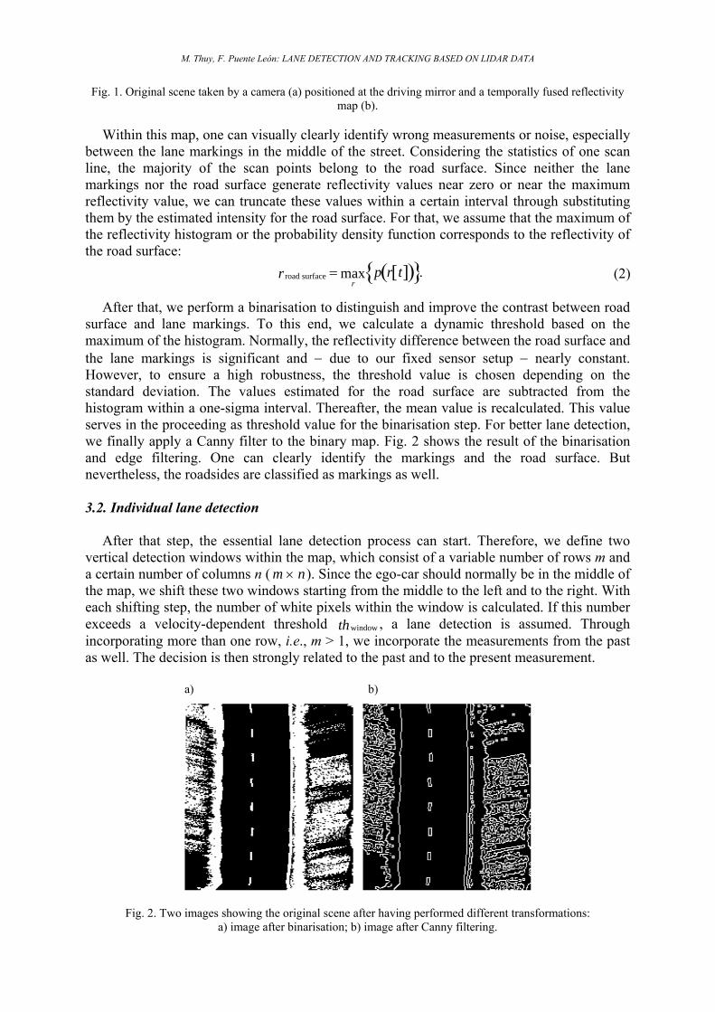
The second strategy is a flexible temporal fusion of the scan data. Fig. 1b shows the reflectivity data from the scanner added line by line over time. In this picture, the data is not registered at all. This leads to the fact that the right curve of Fig. 1a becomes nearly a straight line in Fig. 1b. Another important fact within this map is that the length of the lane markings depends on the ego-speed. As no global registration is performed, the map represents an integration of the environmental scene and the movement of the ego-car. Once again, it has to be emphasized that this spatial adding can only be done without modifying or normalizing reflectivity values, because the distance to the street is almost the same in each row. For a multi-layer scanner, one would have to normalize or to adjust the reflectivity values for scan points according to their varying distance. For illustrating the reflectivity map, we reduced the reflectivity values to one byte (grey values from 0 to 255). Normally, our calculations are based on two-byte values.

a) b)


Fig. 1. Original scene taken by a camera (a) positioned at the driving mirror and a temporally fused reflectivity map (b).

Within this map, one can visually clearly identify wrong measurements or noise, especially

between the lane markings in the middle of the street. Considering the statistics of one scan line, the majority of the scan points belong to the road surface. Since neither the lane markings nor the road surface generate reflectivity values near zero or near the maximum reflectivity value, we can truncate these values within a certain interval through substituting them by the estimated intensity for the road surface. For that, we assume that the maximum of the reflectivity histogram or the probability density function corresponds to the reflectivity of the road surface:

road surfacer =r

max p r t[ ]( ){ }. (2)

After that, we perform a binarisation to distinguish and improve the contrast between road surface and lane markings. To this end, we calculate a dynamic threshold based on the maximum of the histogram. Normally, the reflectivity difference between the road surface and the lane markings is significant and − due to our fixed sensor setup − nearly constant. However, to ensure a high robustness, the threshold value is chosen depending on the standard deviation. The values estimated for the road surface are subtracted from the histogram within a one-sigma interval. Thereafter, the mean value is recalculated. This value serves in the proceeding as threshold value for the binarisation step. For better lane detection, we finally apply a Canny filter to the binary map. Fig. 2 shows the result of the binarisation and edge filtering. One can clearly identify the markings and the road surface. But nevertheless, the roadsides are classified as markings as well. 3.2. Individual lane detection

After that step, the essential lane detection process can start. Therefore, we define two vertical detection windows within the map, which consist of a variable number of rows m and a certain number of columns n ( m × n). Since the ego-car should normally be in the middle of the map, we shift these two windows starting from the middle to the left and to the right. With each shifting step, the number of white pixels within the window is calculated. If this number exceeds a velocity-dependent threshold windowth , a lane detection is assumed. Through incorporating more than one row, i.e., m > 1, we incorporate the measurements from the past as well. The decision is then strongly related to the past and to the present measurement. a) b)

Fig. 2. Two images showing the original scene after having performed different transformations: a) image after binarisation; b) image after Canny filtering.


In the further development, we use these pre-detected lane markings in a consecutive

manner. Based on the current row, we shift again two windows ( 2m × 2n , whereas 2m << 1m ), but this time only in a small region around the pre-detected lane markings. This proceeding ensures that the final decision of a newly detected lane marking is still an individual step (i.e.

2m = 1), which is applied scan by scan, but the past is incorporated as well. Consequently, measurement outliers are efficiently filtered. For the sake of real-time processing, the portion of pre-detection based on the current scan as well as on the past 1m × 1n , and the windowing based on the current frame 2m × 2n

can be adjusted. As the result, integrated errors through

the consecutive detection can be reset by a new pre-detection. a) b)

Fig. 3. Windowing within the binary reflectivity map: a) start of shifting stage; b) end of shifting stage. 4. Data Registration and Global Map

After having detected the lane markings in the current frame, the points can be translated into a fixed-world coordinate system. This way, the effect of the ego-movement is completely suppressed. Since all detected lanes within the reflectivity map are characterized through their relative position in regard to the test car, we transform the lidar points as well as the current ego-position according to formula (1) into the UTM coordinate system. Fig. 4 shows the car and the specific distances.

Fig. 1.Test-car with mounted sensors.

Here, dist t,α[ ]

denotes the appropriate measured distance from the scanner at the angle α.

The INS-point shows the reference point of the car. As we apply pitch compensation, we have to incorporate the pitch difference ∆pitch t[ ]

as well. With origh , i.e., the original height of the


mounted scanner, we can know calculate the current height h[t] caused by the pitch difference by:

h t[ ] = origh − tan ∆pitch t[ ]( )⋅ b . (3)

Now we can infer the distance $a$ by:

a t,α[ ] = sin arccosh t[ ]

dist t,α[ ]

⋅ dist α[ ]. (4)

As we have done so far, we can calculate the point coordinates with respect to the car:

carx t,α[ ]cary t,α[ ]

=

−cos(α)

sin(α)

⋅ a +

0

b

, (5)

and finally apply the transformation to the absolute map coordinates:

mapx

mapy

=

egox t[ ]egoy t[ ]

+ R t[ ]⋅ carx t,α[ ]

cary t,α[ ]

. (6)

Eq. (6) describes the calculation rule for transforming each lidar point, characterized by its

specific angle α and measured distance dist t,α[ ], into a global coordinate system. This proceeding ensures a global description independent of the ego movement. To save calculation time, this transformation is performed only for the detected lane marking points. In order to handle the data efficiently within computer memory, the values are rounded and assigned to the appropriate grid cell. The grid cell dimensions − in our case 1 cm − are adjust-able.

5. The Underlying Lane Model and Parameter Extraction Stage 5.1. The lane model

This paragraph firstly focuses on the assumed lane model. As our central goal is a parametric lane description for attached control modules, an underlying road model has to be defined.

As widely used in literature, we assume a clothoid road model. That means, the road itself forms a clothoid and can therefore be described by a set of clothoid parameters. Starting from the original equation characterizing a clothoid:

x

y

= a π

cosπ 2t2

sinπ 2t2

dt0

k

∫ , k =

l

a π, (7)

one can infer a commonly-used third order polynomial approximation for the x-coordinate parametrized by y:

x ≈ 0x +12

0c2y +

16

1c3y . (8)

For a model with constant curvature, Eq. (8) can be simplified to:


x ≈ 0x +12

0c2y . (9)

Another way to express the road model on a clothoidal basic is a parabolic, polynomial

model:

x ≈ 0A + 1A y + 2A2y , (10)

which does not incorporate the third order component. 5.2. Tracking

Now we have discussed all the ingredients to track the road, i.e., on the one hand the continuous detection of the appropriate lane markings and their transformation into world-fixed coordinates, and on the other hand a suitable road model. Combining these two elements, the road can be fully parametrized by the clothoid parameters. These parameters are based on the present and past lane markings, but with their help one can predict the future course of the lane.

Fig. 5. Schematic overview of the complete tracking procedure.

Since such a prediction always suffers from errors due to mismodeling or measurement noise, the prediction accuracy will be analyzed by comparing the predicted lane to its actual course.

In the following, two different strategies to track the lane will be presented. The first one is based on a least-squares method. The second one is an extended Kalman filter solution, which enables to model both the process and the sensor noise explicitly. 5.2. Least-squares fitting

The central goal of this method is to find the best-approximated curve through the given N sets of coordinates. To find this curve, we have to find a global error measurement:

2χ = iwi=0

N −1

∑2

iy − iY c, ix( )( ) . (11)

Therefore, the accumulative error or the residuum 2χ can be determined by the squared difference of the real y-coordinate iy

and the resulting y-value Y (...) out of the approximation

Eq. (8). iY (K )can now be transferred into a matrix representation:

0 1 2

1 1 1 0

00 1 2

11 1 1

( , ) .

N N N

x x x xccx x x− − −

= ⋅ = Ψ

y c x c (12)

Minimizing Eq. (11) yields the desired parameter vector optc :


optc =−1

TΨ Ψ( ) TΨ y . (13)

This formula can easily be computed by the help of linear algebra libraries. The only computationally crucial parameter is the number N of points. 5.2. Extended Kalman filtering 5.2.1. Process model

Interpreting Eq. (8) as well as Eq. (9) in the sense of a process model, the state variables are 0x , 0c and 1c . This leads to the following expression for the process model:

c k +1[ ] = F⋅ c k[ ]+ σ =1 0 0

0 1 0

0 0 1

⋅

0x k[ ]0c k[ ]1c k[ ]

+xσ

0cσ

1cσ

. (14)

The spatial difference is only modeled by the process noise vector σ. This is intuitively not

obvious. But as we track the road globally, there is no need to change parameters. However, since we cannot model the real road without errors, the parameters will change. 5.2.1. Observation model

In contrary to the just introduced linear process model, the observation model turns out non-linear. This is due to the non-linear clothoid model, which combines the state variables c and the measurement value y:

y k[ ] = H c k[ ],k( )+ w k[ ], (15)

where H(...) represents a time-variant non-linear function. The time-variance is due to the x-

coordinate movement of the ego car, which is inferred by the transformation into global coordinates. The measurement noise is modelled by the noise value w k[ ].

According to the extended Kalman filter proceeding, the scalar function H(...) in equation (15) has to be differentiated and evaluated in the operating point. This leads to the desired time-variant matrix H k[ ]:

H k[ ] =dH c k[ ],k( )

dc . (16)

6. Tracking results

In this section, results corresponding to the overall lane tracking are presented. The performance of the developed tracking system was successfully tested with our test car configuration. The car drove autonomously by controlling its position based on the given clothoidal set of parameters. 6.1. Global map

First of all, we want to show the registered map within fixed-world coordinates. Fig. 6 shows the map on the right side. Within this map, one can notice the real distance between the scanner points due to the fusion with the IMU data. Within the map, the red points marked in red indicate the detected lane. The green dots show the ego-car path.


Fig. 6. Global registered grid. Points in red signal detected lane markings. 6.2. Road parameters

Based on these detected points, we can now apply the polynomial fitting or the Kalman approach to track and extract the lane parameters. To this end, we take the half of the data N/2 = 25 measurements in our example) to feed the tracking method, and the other half to prove the performance of the chosen approach. Within Fig. 7a, the raw data is shown. The blue part of the data serves to feed the tracking, and the red part for the preview.

Fig. 7b shows the result for a polynomial fitting. Fig. 7c shows the result using the presented Kalman filter. Both results show a precise prediction capability, which is sufficient for the attached controller modules, which are responsible to follow the lane. To define a possible measure of error, we use the lateral average error defined by the N/2 predicted road points:

a) b) c)

Fig. 7. Lane tracking results.: a) measured and detected lane data; b) polynomial fitting; c) Kalmann tracking.


( )2

/2 1measure, predicted,

1

i N

i Ni ierr

N x x=

= +

= −∑ , (17)

Using this measure of error, we can determine the resulting error dependent of the chosen

tracking method and the chosen underlying road model. Additionally, we can calculate − according to formula (17) − the error for the past and present value as well. Fig. 8 contrasts the errors. One can clearly identify that the Kalman approach minimizes the error due to explicitly modeling the inherent noise. a) b)

Fig. 8. Average errors. In blue: error based on current and past measurements, in red: error for the lane prediction: a) average errors for Kalmann tracking; b) average errors for polynomial fitting.

7. Conclusion and Outlook

The contribution introduced a lidar-based method to detect and track the lane. The detection is performed independently of continuous or incontinuous lane markings. We showed how a spatio-temporal fusion strategy can serve to accumulate data arising from the one-layer scanner. Within the fused map, one can detect the lane on the basis of current and past information. Parametrizing the detected lane to a widely used clothoidal model closes the article.

In future work, we want to fuse our method with visual sensors. To this end, a fusion scenario at an abstract parameter level can be compared to a low-level signal-based approach. Further, we also will incorporate the information from a laser scanner placed planar to the ground level to detect and track objects, as was shown, e.g., in [9].


Acknowledgment

The authors gratefully acknowledge support of this work by the Deutsche Forschungsgemeinschaft (German Research Foundation) within the Transregional Collaborative Research Centre 28 “Cognitive Automobiles”. References [1] A. Fasoula, H. Driessen, P. van Genderen: “Model-based integrated object tracking and classification”.

Information Fusion, FUSION ’09. 12th International Conference, July 2009, pp. 1006–1013.

[2] M. Meuter, S. Muller-Schneiders, A. Mika, S. Hold, C. Nunn, A. Kummert: “A novel approach to lane detection and tracking”. Intelligent Transportation Systems, ITSC ’09. 12th International IEEE Conference, Oct. 2009, pp. 1–6.

[3] M.J. Jeng, C.Y. Guo, B.C. Shiau, L.B. Chang, P.Y. Hsiao: “Lane detection system based on software and hardware codesign” Autonomous Robots and Agents, ICARA 2009. 4th International Conference, Feb. 2009, pp. 319–323.

[4] K.H. Lim, K.P. Seng, L.M. Ang, S.W. Chin: “Lane detection and kalman-based linear-parabolic lane tracking”. Intelligent Human-Machine Systems and Cybernetics, IHMSC ’09. International Conference, vol. 2, Aug. 2009, pp. 351–354.

[5] M. Thuy, F. Puente León: “An iterative parameter estimation method for observation models with nonlinear constraints”. Metrol. Meas. Syst., vol. XV, no. 4, 2008, pp. 421–432.

[6] P. Lindner, E. Richter, G. Wanielik, K. Takagi, A. Isogai: “Multi-channel lidar processing for lane detection and estimation”. Intelligent Transportation Systems, ITSC ’09. 12th International IEEE Conference, Oct. 2009, pp. 1–6.

[7] K. Takagi, K. Morikawa, T. Ogawa, M. Saburi: “Road environment recognition using on-vehicle lidar”. Intelligent Vehicles Symposium, IEEE, 0-0, 2006, pp. 120–125.

[8] T. Ogawa, K. Takagi: “Lane recognition using on-vehicle lidar”. Intelligent Vehicles Symposium, IEEE, 0-0, 2006, pp. 540–545.

[9] T. Dang: “Non-linear multimodal object tracking based on 2D lidar data”. Metrol. Meas. Syst., vol. XVI, no. 3, 2009, pp. 359–369.

[10] M. Thuy and F. Puente León, “Non-linear, shape independent object tracking based on 2d lidar data”. Intelligent Vehicles Symposium, IEEE, Jun. 2009, pp. 532–537.

[11] M. Thuy, J. Habigt, F. Puente León: “Multi-Objektverfolgung auf der Grundlage von Lidardaten”. XXIII. Messtechnisches Symposium des Arbeitskreises der Hochschullehrer für Messtechnik e.V., AHMT, G. Goch, ed. Aachen, Shaker Verlag, 2009, pp. 181–192.

metrology and measurement systems - kit · m. thuy, f. puente león: lane detection and tracking...

Documents