model based design of electro-hydraulic motion control
TRANSCRIPT

Model Based Design of
Electro-Hydraulic Motion Control Systems
for Offshore Pipe Handling Equipment


Morten Kollerup Bak
Model Based Design of
Electro-Hydraulic Motion Control Systems
for Offshore Pipe Handling Equipment
Doctoral dissertation for the degree of Philosophiae Doctor (Ph.D.) at the
Faculty of Engineering and Science, Specialisation in Mechatronics
University of Agder
Faculty of Engineering and Science2014
iii

Doctoral Dissertation by the University of Agder 85
ISBN: 978-82-7117-764-5
ISSN: 1504-9272
c©Morten Kollerup Bak, 2014
Printed in the Printing Office, University of Agder
Kristiansand
iv

Preface
This dissertation contains the essential results of the research I carried out in my Ph.D.
project at the Department of Engineering Sciences, Faculty of Engineering and Science,
University of Agder. The research was carried out in close cooperation with Aker So-
lutions in Kristiansand in the period between December 2009 andDecember 2013. The
project was funded by the Norwegian Ministry of Education and Research and co-funded
by Aker Solutions.
I owe my deepest gratitude to my supervisor Prof. Michael Rygaard Hansen for his
encouragement and guidance throughout the project. He has always been ready to moti-
vate me and guide me on the right path whenever it was needed andI could not imagine
having a better advisor for my work. I would like to thank Aker Solutions for giving me
the possibility to work on an exciting project with industrial applications - it has been
a great learning experience. I would especially like to thank Pål Andre Nordhammer
(Aker Solutions) for his invaluable input and ideas which indeed helped shaping the
project.
During the past four years I have met and gotten to know a lot of people who have helped
and inspired me in one way or another. I don’t know how to thankall these people - their
names are far too many to mention here and I’m afraid I will forget someone.
Without mentioning any names I would first of all like to thankmy former colleagues
in the mechatronics group at the University of Agder. They provide a fun, creative and
friendly working environment and are always forthcoming when asked for help. I would
also like to thank all my colleagues from Aker Solutions who have helped me during the
project. Their help has enabled me to achieve unique resultsand has quite simply been
invaluable to me.
Perhaps most importantly, I would like to thank all my fellowPh.D. students at the Uni-
versity of Agder - both within and outside the mechatronics group. Some of them started
before me and finished before I did. Some of them started afterme and have yet to finish.
A few of them even started after I did and finished before me. They provided a very nice
and fun social environment that has left me with unforgettable memories.
I would also like to thank my former fellow students from Aalborg University in Den-
mark who formed their own network of Ph.D. students and invited me to join. The last
five years or so we have met once or twice a year to discuss our research and, not least,
to socialize and catch up. These meetings have been a great motivation and inspiration
to me and have always brought fun and good times.
v

The past four years have been exciting and enriching, but also tough and filled with
tremendous workloads. At times I have felt I was losing my mindout of sheer stress,
too much coffee and too little sleep. But during these four years I have met a lot of nice
people from all over the world and travelled to places I neverthought I would go - all
while working with what I think is the most interesting. If that is not a privilege I don’t
know what is.
Morten Kollerup Bak
Grimstad, Norway
January 2014
vi

Summary
Despite the fact that hydraulics, in general, is considered amature technology, design
of hydraulic systems still offers a number of challenges forboth component suppliers
and manufacturers of hydraulically actuated machines suchas offshore pipe handling
equipment. This type of equipment is characterized by high price, high level of system
complexity and low production numbers. It requires a great level of skill and expe-
rience to develop the equipment and the focus on production and development costs
is constantly increasing. Therefore design engineers continuously have to improve their
procedures for decision making regarding choice of principal solutions, components and
materials in order to reach the best possible trade-off between a wide range of design
criteria as fast as possible.
In this dissertation methods for modeling, parameter identification, design and optimiza-
tion of a selected piece of offshore pipe handling equipment, a knuckle boom crane, are
put forward and treated in details in five appended papers.
Modeling of mechanical multi-body systems with attention tostructural flexibility is
treated in papers I and IV. Modeling, testing and parameter identification of directional
control valves with main focus on dynamic characteristics are treated in paper II and also
discussed in papers III and IV. Modeling of counterbalance valves with main focus on
steady-state characteristics is treated in papers III and IV. In paper IV also modeling of
hydraulic cylinders is discussed and a procedure for parameter identification for models
of hydraulic-mechanical systems is presented.
Steady-state design procedures for hydraulic systems are discussed in paper III and a
design optimization method for reduction of oscillations is presented. Paper V deals
with dynamic considerations in design of electro-hydraulicmotion control systems for
offshore pipe handling equipment.
All the presented methods are developed to accommodate the needs of the system de-
signer. They take into account the limited access to component data and time available
for model development and design optimization, which are themain challenges for the
system designer. The methods also address the problem of required knowledge within
several disciplines, e.g., by suggesting modeling assumptions and experimental work
suitable for system design.
vii

viii

Contents
Publications xi
1 Introduction 1
1.1 Motivation and Background . . . . . . . . . . . . . . . . . . . . . . . 3
1.2 State of the Art . . . . . . . . . . . . . . . . . . . . . . . . . . . . . . 5
2 Offshore Pipe Handling Equipment 9
2.1 The Knuckle Boom Crane . . . . . . . . . . . . . . . . . . . . . . . . 11
3 Modeling and Parameter Identification 15
3.1 Mechanical Systems . . . . . . . . . . . . . . . . . . . . . . . . . . . 17
3.2 Hydraulic Components and Systems . . . . . . . . . . . . . . . . . . . 19
4 Design and Optimization 23
4.1 Hydraulic System Design . . . . . . . . . . . . . . . . . . . . . . . . . 24
4.2 Use of Simulation Models . . . . . . . . . . . . . . . . . . . . . . . . 24
5 Conclusions 29
5.1 Contributions . . . . . . . . . . . . . . . . . . . . . . . . . . . . . . . 29
5.2 Outlook . . . . . . . . . . . . . . . . . . . . . . . . . . . . . . . . . . 31
References 33
Appended papers 40
ix

I A Method for Finite Element Based Modeling of Flexible Components in
Time Domain Simulation of Knuckle Boom Crane 41
II Modeling, Performance Testing and Parameter Identification of
Pressure Compensated Proportional Directional Control Valves 57
III Model Based Design Optimization of Operational Reliability in
Offshore Boom Cranes 79
IV Analysis of Offshore Knuckle Boom Crane — Part One:
Modeling and Parameter Identification 111
V Analysis of Offshore Knuckle Boom Crane — Part Two:
Motion Control 147
x

Publications
The following five papers are appended and will be referred to bytheir Roman numerals.
The papers are printed in their originally published state except for changes in format
and minor errata.
I J. Henriksen, M. K. Bak and M. R. Hansen, “A Method for Finite ElementBased
Modeling of Flexible Components in Time Domain Simulation of Knuckle Boom
Crane”,The 24th International Congress on Condition Monitoring and Diagnos-
tics Engineering Management, pp. 1215-1224. Stavanger, Norway, May 30 - June
1, 2011.
II M. K. Bak and M. R. Hansen, “Modeling, Performance Testing and Parameter
Identification of Pressure Compensated Proportional Directional Control Valves”
The 7th FPNI PhD Symposium on Fluid Power, pp. 889-908. Reggio Emilia, Italy,
June 27 - 30, 2012.
III M. K. Bak and M. R. Hansen, “Model Based Design Optimization of Operational
Reliability in Offshore Boom Cranes”,International Journal of Fluid Power. Vol.
14 (2013), No. 3, pp. 53-65.
IV M. K. Bak and M. R. Hansen, “Analysis of Offshore Knuckle Boom Crane —
Part One: Modeling and Parameter Identification”,Modeling, Identification and
Control. Vol. 34 (2013), No. 4, pp. 157-174.
V M. K. Bak and M. R. Hansen, “Analysis of Offshore Knuckle Boom Crane— Part
Two: Motion Control”,Modeling, Identification and Control. Vol. 34 (2013), No.
4, pp. 175-181.
The following papers are not included in the dissertation butconstitute an important part
of the background.
xi

VI M. K. Bak, M. R. Hansen and P. A. Nordhammer, “Virtual Prototyping - Model
of Offshore Knuckle Boom Crane”,The 24th International Congress on Condition
Monitoring and Diagnostics Engineering Management, pp. 1242-1252. Stavanger,
Norway, May 30 - June 1, 2011.
VII M. K. Bak, M. R. Hansen and Karimi, H. R., “Robust Tool Point Control for
Offshore Knuckle Boom Crane”,The 18th World Congress of the International
Federation of Automatic Control (IFAC), pp. 4594-4599. Milano, Italy, August 28
- September 2, 2011.
VIII P. A. Nordhammer, M. K. Bak and M. R. Hansen, “A Method for Reliable Mo-
tion Control of Pressure Compensated Hydraulic Actuation with Counterbalance
Valves”,The 12th International Conference on Control, Automation and Systems,
pp. 759-763. Jeju Island, Korea, October 17 - 21, 2012.
IX P. A. Nordhammer, M. K. Bak and M. R. Hansen, “Controlling the Slewing Motion
of Hydraulically Actuated Cranes Using Sequential Activation ofCounterbalance
Valves”,The 12th International Conference on Control, Automation and Systems,
pp. 773-778. Jeju Island, Korea, October 17 - 21, 2012.
xii

Chapter 1Introduction
Offshore drilling for oil and gas production dates back to theend of the nineteenth cen-tury and began with drilling in fresh water lakes as well as shallow salt waters at thecoast of California. During the 1960’s, 70’s and 80’s drilling moved into areas of harshenvironments, like the North Sea, and so-called deepwater (water depths between 500and 1500 m) in the Gulf of Mexico. This development still continues today with drillingin arctic areas and ultra deepwater (water depths beyond 1500 m).Naturally, this has required and led to a major development ofboth subsea equipment,e.g., for well control, and topside equipment such as top drives (drilling machines), hoist-ing systems and pipe handling equipment. The fact that drilling is constantly moving to-wards harsher environments and deeper waters obviously increases the requirements forthe equipment being used. This again leads to a number of challenges for the offshoreequipment manufacturers.For applications such as top drives and hoisting systems themost noticeable design chal-lenge is the increase in required lifting capacity. Today the required lifting capacity oftenreaches as high as 1500 short tons and in some cases even beyond. In addition, motioncompensation is required for hoisting systems whenever usedon a floating installation.For offshore equipment in general, due to remote locations and high cost of down time,reliability and productivity are the most important performance criteria. Therefore de-sign is based on well proven solutions and development of the equipment has been asteady process with incremental improvements of functionality and performance. Dur-ing the last couple of decades machine development has primarily been concentratedaround control systems technology which has led to significant development in automa-tion and safety of machine operations. In terms of technology, structural design and de-sign of actuation systems have developed at a much slower ratewith only minor develop-ments of materials and components. However, the development of PCs and CAD/CAEsystems has had a significant impact on how design engineers work and has enabled
1

2 Model Based Design...
design improvements based on the existing technology.Besides most types of top drives and hoisting systems, topside equipment such as pipehandling equipment normally rely on hydraulic or electro-hydraulic actuation. The rea-son for this is that hydraulic actuation is a well-proven, reliable and robust solution witha number of advantages compared to electrical actuation. Among others, these advan-tages include:
• Heat transfer. The hydraulic fluid carries away generated heat to a convenientheat exchanger. This allows for smaller and lighter components.
• Lubrication . The hydraulic fluid acts as a lubricant and facilitates long componentlife.
• Power density. Torque/force developed by a hydraulic actuator is proportionalto pressure difference and only limited by permissible stress levels. With respectto size and weight, hydraulic actuators deliver high effort compared to electricalactuators.
• Price. Today hydraulic components are relatively cheap comparedto many elec-trical components.
Furthermore, there is a vast amount of experience with hydraulic actuation in the off-shore industry and far less experience with electrical actuation. Therefore a changeof technology is complicated and represents a relatively high risk even though electricdrives have developed significantly over the past decades. Naturally, hydraulic actuationis also associated with a number of disadvantages such as:
• Contamination. Contaminated oil can clog valves and actuators or cause wearwhich leads to permanent loss in performance or failure. Contamination is themost common source of failure in hydraulic systems.
• Efficiency. Hydraulic systems normally have quite poor efficiencies compared toelectrical systems.
• System complexity. Hydraulic systems often require more components than elec-trical systems which increases the system complexity. Furthermore, the need forpassive control elements such as counterbalance valves often introduces instabilityand lowers the overall efficiency.
Some of these disadvantages may be eliminated by introducing more modern technolo-gies such as separate meter-in separate meter-out control (Eriksson and Palmberg, 2011),digital hydraulics (Linjama and Vilenius, 2007) or integrated actuators (Michel and We-ber, 2012) which have yet to be adopted by the offshore industry. The reason these

Introduction 3
technologies have not yet been applied is that they are less field proven and thereforerepresent less reliable solutions.Hydraulics, or fluid power in general, is a widely used technology with application to,e.g., the automotive and the aerospace industries, off-highway vehicles, wind turbinesand production and manufacturing machines. Hydraulics is often divided into two cat-egories;mobile hydraulicsmainly referring to off-highway applications andindustrialhydraulicsmainly referring to production and manufacturing applications. Industrialapplications are typically characterized by high requirements for repeatability, dynamicresponse and accuracy whereas mobile applications often have high requirements forversatility and human-machine interface. Furthermore, industrial application are usu-ally supplied by a constant pressure system whereas mobile applications usually aresupplied by a system with variable supply pressure (load sensing systems).In terms of requirements for repeatability, dynamic response and accuracy as well asversatility and human-machine interface, offshore applications are located somewherebetween mobile and industrial applications. They are usually supplied by constant pres-sure systems, but use components from both mobile and industrial applications.Although electric drives and modern fluid power technologies certainly will gain moreground in the offshore industry, a sudden change in actuation technology seems unlikely.Therefore maintenance and development of knowledge within design of hydraulic sys-tems is highly relevant and will continue to be for decades to come.
1.1 Motivation and Background
Despite the fact that hydraulics, in general, is considered amature technology, designof hydraulic systems still offers a number of challenges forboth component suppliersand manufacturers of hydraulically actuated machines suchas offshore pipe handlingequipment. This type of equipment is characterized by high price, high level of systemcomplexity and low production numbers. It requires a great level of skill and expe-rience to develop the equipment and the focus on production and development costsis constantly increasing. Therefore design engineers continuously have to improve theirprocedures for decision making regarding choice of principal solutions, components andmaterials in order to reach the best possible trade-off between a wide range of designcriteria as fast as possible.For hydraulic and electro-hydraulic actuation systems, most design challenges are re-lated to the dynamics of the actuation system and the application it is being designedfor. While design procedures based on steady-state considerations are well-known andfairly easy to apply, there is still a lack of robust design procedures that take the sys-tem dynamics into account. This includes both stability andaccuracy, i.e., the systems

4 Model Based Design...
tendency to oscillate and ability to follow a reference signal. These criteria are not eas-ily evaluated and are therefore often left unaddressed until the system has been realizedand can be tested. Although, in practice, a substantial amount of tuning is usually re-quired, insufficient focus on dynamics during the design phase often leads to costly andtime consuming design changes which can be difficult to implement after the system hasbeen realized. This is especially problematic for areas like the offshore industry wherethere are very limited opportunities to build prototypes for verification of a new design.The problem calls for a model based approach which enables thedesigner to evaluate thesystem dynamics and take measures to improve it before the system is build. Non-lineardynamic models may be linearized and used to check for stability in selected operatingpoints and to analyze how system parameters influence the stability margin. However foranalysis of complete operating cycles it quickly becomes impractical to work with lin-earized models. Furthermore, since stability is an absolute measure and many hydraulicsystems are likely to become unstable in one or more operating points or oscillate inlimit cycles, it is more meaningful to consider the level of oscillations occurring duringthe operating cycle.What is needed for more detailed system analysis is dynamic time domain simulationwhich can be used to analyze both oscillation level and accuracy during the operatingcycle in order to evaluate the system design and possibly carry out design optimization.A model based design approach may be illustrated as in Fig. 1.1.
Dynamic Model
Actuation System
Mechanical System
ControlSystem
Design/Optimization Procedure
Design parameters
Simulation results
Figure 1.1: Model based design approach.
Depending on the purpose, a more or less extensive model of theconsidered system isneeded. For design of motion control systems for applications like offshore pipe han-dling equipment, rather detailed models including the mechanical system, the actuationsystem and the control system are usually required. In addition, environmental effectsand even operator behavior may need to be considered.Simulation models serve as virtual prototypes providing information about machine per-

Introduction 5
formance such as overall efficiency, oscillatory behavior and accuracy, enabling engi-neers to test, redesign and optimize the design before it is manufactured. This may bedone by either using the model directly as a design evaluation tool or by coupling it witha numerical optimization routine.One of the major challenges in model based design is to producesimulation modelsthat, with a reasonable precision, are able to mimic the behavior of a real system. Thischallenge is especially pronounced for hydraulically actuated machines simply becausesuppliers of hydraulic components are not used to deliver all the data needed to developsimulation models of their products.The challenges of model based design may be divided into three categories:
• Modeling and simulation. This includes choice of simulation software, modelingtechniques and level of modeling detail.
• Model validation and verification. This usually involves some sort of experi-mental work followed up by parameter identification.
• Use of simulation models. This includes setting up a suitable frame work for post-processing of simulation results and optimization of critical design parameters.
These topics form the basis for the work presented in this dissertation and are treatedin more detail in chapters 3 and 4 and are also subjected to a literature review in thefollowing section.
1.2 State of the Art
Fluid power technology is a relatively small research area, but even so hydraulics hasbeen subject to extensive research during both the past and the current century. Anoverview of relatively recent research issues is given by Burrows (2000). The technol-ogy, as we know it today, has been around for at least a century and has gone througha slow and steady development with research results remaining relevant for a long time.An example of that is the work by Merritt (1967), which is still frequently referred to inboth research and education and by practicing engineers.During the recent decades, with the development of PCs and commercially availablesoftware for simulation and technical computing, design and optimization of hydraulicsystems has attracted a considerable amount of interest from researchers in the fluidpower community. Fundamental design procedures based on steady-state based con-siderations have been presented by Stecki and Garbacik (2002). System design andcomponent selection using dynamic simulation and numerical optimization has been in-vestigated by Krus et al. (1991), Andersson (2001), Hansen and Andersen (2001), Krim-

6 Model Based Design...
bacher et al. (2001), Papadopoulos and Davliakos (2004), Pedersen (2004) and Hansenand Andersen (2005).Conceptual design and so-called expert systems for automated design have also attracteda considerable amount of attention, (Dunlop and Rayudu, 1993), (Lin and Shen, 1995),(da Silva and Back, 2000), (da Silva, 2000), (Darlington et al., 2001), (Hughes et al.,2001), (Liermann and Murrenhoff, 2005), (Steiner and Scheidl, 2005), (Schlemmer andMurrenhoff, 2008) and (Engler et al., 2010). The impact outside academia, however,remains limited. A reason for this may be that design of hydraulic systems is some-what application dependent. Design criteria and constraintsin combination with designtraditions differ from one application area to another, making it difficult to set up andmaintain design rules for expert systems. Moreover, skepticism and conservatism maycontribute to design engineers being reluctant to make use of such systems.Hydraulic systems are therefore still designed manually andmost often based on exist-ing systems, reducing the design job to a sizing problem wherethe system architectureis already given. In these cases the design engineer can certainly benefit from tools suchas dynamic simulation and optimization. This has already been pointed out by Palmberg(1995) and demonstrated by Hampson et al. (1996).Computer based time domain simulation and optimization techniques have, by far, proventhemselves as excellent tools for the challenged designer and have over the last coupleof decades increasingly been employed by drilling equipment manufacturers. However,the use of these techniques still offers a number of challenges both in industry as wellas academia. As previously mentioned, the main challenge is to produce reliable simu-lation models that can be used for design purposes.Today there are several commercially available software packages for modeling andsimulation of multi-domain systems. Many of these softwarepackages include exten-sive libraries of generic model components making it easy and fast to develop modelsof control systems and hydraulic-mechanical systems and tocombine sub-models ofdifferent physical domains. However, efficient modeling still requires a great level oftheoretical knowledge and experience within specific disciplines.For modeling of mechanical systems the use of three-dimensional multi-body model-ing techniques, (Nikravesh, 1988), (Eberhard and Schiehlen, 2006), (Schiehlen, 1997),(Schiehlen, 2007) and (Yoo et al., 2007), is especially challenging. This is mainly relatedto modeling of structural flexibility, although this has been subjected to quite extensiveresearch, (Shabana, 1997), (Pascal, 2001), (Braccesi et al., 2004), (Bouzgarrou et al.,2005), (Gerstmayr and Schöberl, 2006), (Munteanu et al., 2006), (Bauchau et al., 2008)and (Naets et al., 2012). Many of the modern techniques are based on finite element(FE) formulations and are not always possible to apply when using multi-domain sim-ulation software packages. Therefore lumped parameter approaches such as those usedby Banerjee and Nagarajan (1997), Hansen et al. (2001) and Raman-Nair and Baddour

Introduction 7
(2003) are also highly relevant because they are easy to implement and require relativelylittle computational effort while offering accuracy that issufficient for many purposes.Lumped parameters techniques for modeling of structural flexibility and damping arediscussed in section 3.1.For modeling of hydraulic components and systems, challenges are first of all related tothe fact that model parameters are difficult to acquire or notavailable at all. Thereforeexperimental work is often required and certain model structures have to be assumedwhich allow for simplifications without ignoring or underestimating important physicalphenomena. These challenges are especially pronounced forcomponents such as cylin-ders, directional control valves and pressure control valves like counterbalance valves.Modeling of friction is a well-documented topic, (Bo and Pavelescu, 1982), (Armstrong-Hélouvry et al., 1994), (Olsson et al., 1998) and (Maré, 2012).Friction in hydrauliccylinders has been investigated several times and quite accurate models have been de-veloped, (Bonchis et al., 1999), (Yanada and Sekikawa, 2008), (Márton et al., 2011),(Ottestad et al., 2012) and (Tran et al., 2012). However the number of required modelparameters represents a problem because they cannot be determined without experimen-tal work. Consequently, simpler model often have to be used which, naturally, neglectscertain physical phenomena but nevertheless are sufficientfor most design purposes.This is further discussed in section 3.2.Modeling of spool type directional control valves is also quite well documented and hasbeen investigated, e.g., by Handroos and Vilenius (1991), Käppi and Ellman (1999),Käppi and Ellman (2000), Gordic et al. (2004), Nielsen et al. (2006) and Maré and Attar(2008). Other types of flow control valves and pressure control valves have been inves-tigated by Zhang et al. (2002), Muller and Fales (2008), Opdenbosch et al. (2009), Ruanet al. (2001) and Alirand et al. (2002). Modeling of hydraulicvalves is often problematicdue to the limited information available from datasheets and due to physical phenom-ena such as friction and resulting hysteresis, nonlinear discharge area characteristics,varying discharge coefficients and varying flow forces. Computational fluid dynamics(CFD) may be used to provide insight in some of these phenomena, but often experi-mental work and semi-physical or non-physical modeling approaches are required fortime domain simulation. This is addressed in further details in section 3.2.Today there are no rules for selection of components, designoptimization and model-ing of hydraulically actuated machines like offshore pipe handling equipment. In thisdissertation contributions in these areas are put forward and treated in details in the fiveappended papers.Modeling of mechanical multi-body systems with attention tostructural flexibility istreated in papers I and IV. Modeling, testing and parameter identification of directionalcontrol valves with main focus on dynamic characteristics are treated in paper II and alsodiscussed in papers III and IV. Modeling of counterbalance valves with main focus on

8 Model Based Design...
steady-state characteristics is treated in papers III and IV. In paper IV also modeling ofhydraulic cylinders is discussed and a procedure for parameter identification for modelsof hydraulic-mechanical systems is presented.Steady-state design procedures for hydraulic systems are discussed in paper III and adesign optimization method for reduction of oscillations is presented. Paper V dealswith dynamic considerations in design of electro-hydraulicmotion control systems foroffshore pipe handling equipment.All the presented methods are developed to accommodate the needs of the system de-signer. They take into account the limited access to component data and time availablefor model development and design optimization, which are themain challenges for thesystem designer. The methods also address the problem of required knowledge withinseveral disciplines, e.g., by suggesting modeling assumptions and experimental worksuitable for system design.

Chapter 2Offshore Pipe Handling Equipment
Offshore drilling rigs include a wide range of highly specialized machines, which areused to perform different operations, see Fig. 2.1. Besidesthe top drive and the hoistingsystem, topside equipment may be divided into the following categories:
• Drill floor equipment . This includes machines such as the roughneck, which isused to connect and disconnect the drill pipes that make up thedrill string.
• Pipe handling equipment. This includes a number of different handling tools andcrane types, which are used to handle and transport drill pipes and risers betweendifferent locations on the rig.
• BOP handling equipment. This is used to handle the blowout preventer (BOP).
• Compensaters and tensioners. Compensators include both passive and activeheave compensation equipment and are used to either maintain aconstant weighton bit (WOB) while drilling or keeping the top drive in a fixed position while therig is moving. Tensioners are used to maintain a constant tension in the riser toavoid buckling while the rig is moving.
• Mud pumps and drilling fluid handling systems. Mud pumps are used to pumpdrilling mud into the well while drilling in order to cool and lubricate the drill bitand to carry cuttings from the well to the top side where it is separated from themud by the drilling fluid handling system.
• Hydraulic power units . These are used to supply fluid power to the hydraulicallyactuated machines onboard the rig.
• Control and monitoring system. This is used to control and monitor the equip-ment and the drilling process.
9

10 Model Based Design...
Knuckle boom crane
Pipe deckRiser handling
crane
Riser storage area
Vertical pipe handling crane
Setback area
Drill floor
Top drive
Horizontal-to-vertical pipe handling crane
Riser tensioning system
Heave compensation system
Figure 2.1: Typical drilling rig layout.Image courtesy of Aker Solutions.
On a typical drilling rig, the pipe handling equipment consists of a knuckle boom craneand a tubular feeding machine which are used to transport drill pipes between the pipedeck and the drill floor. On the drill floor there is usually a horizontal-to-vertical pipehandling crane, a so-called mousehole and vertical pipe handling system which are allused to build stands (assemblies of either three or four drill pipes) and to transport thestands between the setback area and the well center.The riser elements are transported between the riser storagearea and the drill floor bymeans of a riser handling crane, a riser chute and a manipulator arm located on the drillfloor.

Offshore Pipe Handling Equipment 11
2.1 The Knuckle Boom Crane
For the design engineer, the knuckle boom crane is a challenging application because itsdynamic characteristics change significantly with the operating conditions, e.g., size ofpayload and position and speed of the actuators of the crane.Knuckle boom cranes are used for a wide range of offshore and marine operations andtherefore exist in different variations. The cranes used for pipe handling typically havethree booms or jibs as the one shown in Fig. 2.2 and the one considered in paper IV, butmay also have of only two jibs as the one considered in paper I.
Figure 2.2: Pipe handling knuckle boom crane.Image courtesy of Aker Solutions.
The crane may be treated as a large multi-domain system consisting of three interactingsystems:
1. A mechanical system.
2. An electro-hydraulic actuation system.
3. An electronic control system.

12 Model Based Design...
The mechanical system provides the geometric and structural properties of the cranewhile the other two systems constitute the motion control system. The main compo-nents of the mechanical system are a rotating part mounted ona pedestal with a slewingbearing and either two or three crane jibs and a gripping yokeconnected in series bymeans of hinges. The crane is controlled from the operator’scabin mounted on the ro-tating part, also called the king.The actuation system consists of several hydraulic circuits supplied by a hydraulic powerunit (HPU) with constant supply and return pressures,pS and pR. Together with thecontrol system, the circuits of the actuation system make upa number of motion controlsub-systems, each controlling one degree of freedom (DOF). A simplified schematic ofa typical motion control sub-system is shown in Fig. 2.3.
pS
pR
DCV
CBV
uJS
uv
yFBC
FFC
yref
vref
SPG
uFF
uFB
p2
p1
p3
pLSpcomp
e
Figure 2.3: Typical motion control sub-system.
The illustrated circuit is used to control the inner jib of the crane and consists of acylinder with integrated position sensor, a counterbalancevalve (CBV) and a directionalcontrol valve (DCV) as the main components of the actuation system.The cylinder motion is controlled with the DCV, which controls the flow into either ofthe two cylinder chambers. When the cylinder is exposed to negative loads (piston ve-locity and load force have the same direction), also the outlet pressure of the cylinderneeds to be controlled. This is normally handled by the CBV, which provides a reliefvalve functionality on the outlet side of the cylinder assisted by the pressure on the inletside. Negative loads occur during load lowering and can occur in both directions of mo-tion for cylinders controlling the intermediate and outer jibs. In these cases CBVs arerequired on both the piston side and the rod side of the cylinder.

Offshore Pipe Handling Equipment 13
This is also required for motor circuits such as the one controlling the slewing motionof the crane where the inertia load needs to be controlled. CBVsexist in different vari-ations, e.g., externally vented, non-vented and relief compensated, due to the differentapplications they are used for.Most often a pressure compensated DCV with electro-hydraulicactuation and closedloop spool position control is used. The reason for this is that it provides load inde-pendent flow control which reduces the requirements for the control system and makesit easier to tune the controller gains. Furthermore, load independent flow control isrequired whenever an operator is to control more than one DOF at the time without as-sistance from the control system.Offshore knuckle boom cranes generally feature a high degreeof automation comparedto other types of cranes. The control strategy relies on position and/or velocity feedbackfrom the individual DOFs. The control system consists of four elements:
• Human-machine interface (HMI)
• Set point generator (SPG).
• Feedforward controller (FFC).
• Feedback controller (FBC).
Besides monitors, push buttons and switches, the HMI containstwo joysticks which theoperator uses to generate command signals for the control system. Joystick signals arefed to the SPG where they may be treated in different ways depending on the selectedcontrol mode. In open loop control mode the joystick signal,uJS, is fed directly to theDCV as a feedforward signal, see Fig. 2.3. In closed loop control mode joystick signalsare transformed into velocity and position references for the individual cylinder motions.The latter is used for path control of the crane’s gripping yoke where several DOFs arecontrolled in a coordinated manner.The FFC is a scaling of the velocity reference,vre f and the FBC is usually a PI controllerwhich compensates for disturbances and accumulated position errors,e= yre f −y. Thecontrol system usually also contains an element which compensates for deadband of theDCV. The system architecture shown in Fig. 2.3 is a popular structure because of itssimple and, consequently, robust design. Furthermore, thecontrollers are easy to tunebecause of the load independent flow control.

14 Model Based Design...

Chapter 3Modeling and Parameter Identification
Even though techniques have been around for several decades, modeling for dynamicsimulation has become significantly easier during the last decade alone. Today there ex-ists a number of commercially available software packages such as MATLAB/Simulink,SimulationX, AMESim, Dymola, Maple/MapleSim and 20-sim, which can be used fortime domain simulation of multi-domain systems such as hydraulic-mechanical systems.All these software packages are based on graphical environments in which models aredeveloped simply by drag-and-drop and connection of generic model components fromthe integrated model libraries.Most of the tools also facilitate development of user-defined model components, whichis often required for modeling of hydraulic components. Furthermore, with standardslike the Modelica language and functional mock-up interface (FMI) models can be ex-changed and used with several different simulation tools, making simulation more plat-form independent.For the work presented in this dissertation, several different software packages have beenused. For the work in paper I, SimulationX is used for modeling and simulation and forthe remaining papers Maple/MapleSim is used. In papers II, III, IV and V also MAT-LAB/Simulink is used for different purposes.In model based design the actual modeling is closely linked to the design objectives.The main challenge is to minimize the complexity of the modelswithout ignoring orunderestimating important physical phenomena. Put in another way, models must be assimple as possible and as detailed as required.For system designers this challenge involves setting up suitable models of mechanicalstructures and sub-supplier components for which the required data may be difficult toacquire or not available. This is especially pronounced forhydraulic components andtherefore experimental work may be required to identify missing models parameters.As time, resources and practical circumstances seldom allowfor full-scale experimental
15

16 Model Based Design...
work for verification of complete system model, testing and experimental work may becarried out with partial systems or separate components for verification of sub-models.Testing and model parameter identification of DCVs and CBVs is treated in papers IIand IV, respectively, and in paper IV an approach for experimental model verificationof a complete crane model is described. The approach involves three steps where thefirst is to consider the steady-state forces on the actuatorsin order to tune the masses andcenters of gravity of the bodies of the mechanical model and to identify friction param-eters for the actuators. In the second step steady-state pressures are considered in orderto tune steady-state characteristics of the valves of the hydraulic model. In the third stepthe system dynamics, i.e., vibration frequencies and vibration levels, are considered inorder to tune mechanical and hydraulic flexibility and damping.In general the calibration and verification of a model can be illustrated as in Fig. 3.1.
Input Measured output
Simulated output
Measured state variables
Simulated state variables
Model
Real system
No Yes Verified
New simulation with new parameters
Correspondence?
Figure 3.1: Principle of model verification.
In order to calibrate and verify the model, the inputs from the experiments are fed tothe model and the uncertain parameters are systematically tuned (identified) until bothsimulated outputs and state variables correspond to those obtained in the experiments.This is described in further details in paper IV.Model verification is closely related to model validation, and although the meaningsof the two terms are different they are often used interchangeably. Model verificationis concerned with implementation of the model and whether the model parameters arecorrect. Model validation, on the other hand, is concerned with the model structureand whether the model is an accurate representation of the real system being consid-ered. Consequently, if the model verification, i.e., parameters identification, fails thenthe model validation also fails and the model structure needs to be reconsidered.
Modeling and Model Verification 17
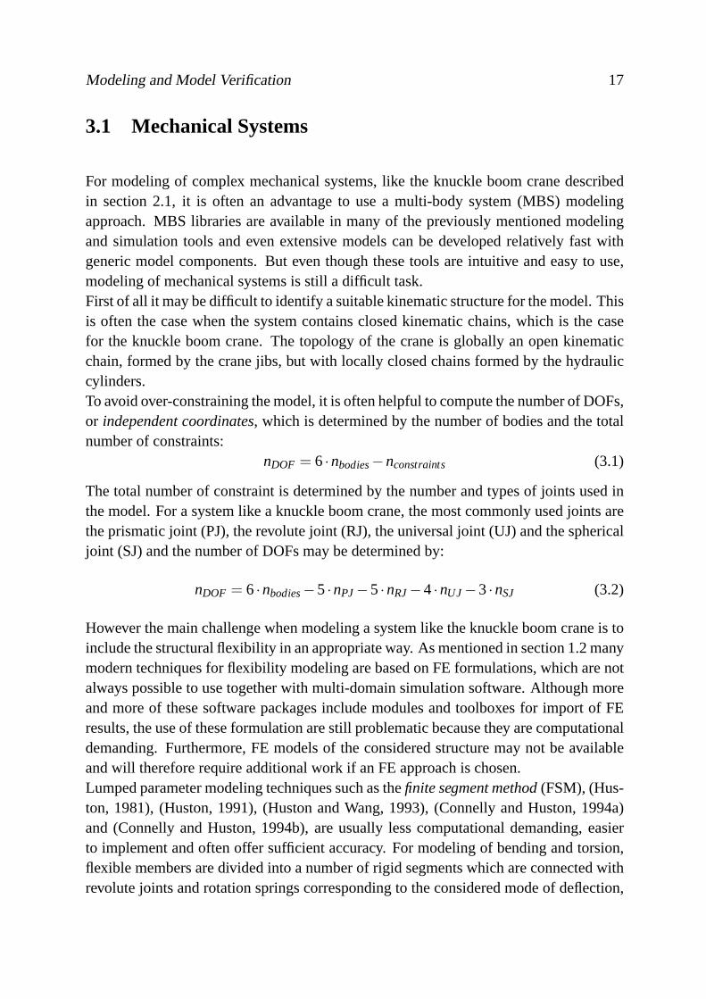
3.1 Mechanical Systems
For modeling of complex mechanical systems, like the knuckle boom crane describedin section 2.1, it is often an advantage to use a multi-body system (MBS) modelingapproach. MBS libraries are available in many of the previously mentioned modelingand simulation tools and even extensive models can be developed relatively fast withgeneric model components. But even though these tools are intuitive and easy to use,modeling of mechanical systems is still a difficult task.First of all it may be difficult to identify a suitable kinematic structure for the model. Thisis often the case when the system contains closed kinematic chains, which is the casefor the knuckle boom crane. The topology of the crane is globally an open kinematicchain, formed by the crane jibs, but with locally closed chains formed by the hydrauliccylinders.To avoid over-constraining the model, it is often helpful tocompute the number of DOFs,or independent coordinates, which is determined by the number of bodies and the totalnumber of constraints:
nDOF = 6 ·nbodies−nconstraints (3.1)
The total number of constraint is determined by the number and types of joints used inthe model. For a system like a knuckle boom crane, the most commonly used joints arethe prismatic joint (PJ), the revolute joint (RJ), the universal joint (UJ) and the sphericaljoint (SJ) and the number of DOFs may be determined by:
nDOF = 6 ·nbodies−5 ·nPJ−5 ·nRJ−4 ·nUJ−3 ·nSJ (3.2)
However the main challenge when modeling a system like the knuckle boom crane is toinclude the structural flexibility in an appropriate way. As mentioned in section 1.2 manymodern techniques for flexibility modeling are based on FE formulations, which are notalways possible to use together with multi-domain simulation software. Although moreand more of these software packages include modules and toolboxes for import of FEresults, the use of these formulation are still problematicbecause they are computationaldemanding. Furthermore, FE models of the considered structure may not be availableand will therefore require additional work if an FE approach is chosen.Lumped parameter modeling techniques such as thefinite segment method(FSM), (Hus-ton, 1981), (Huston, 1991), (Huston and Wang, 1993), (Connellyand Huston, 1994a)and (Connelly and Huston, 1994b), are usually less computational demanding, easierto implement and often offer sufficient accuracy. For modeling of bending and torsion,flexible members are divided into a number of rigid segments which are connected withrevolute joints and rotation springs corresponding to the considered mode of deflection,

18 Model Based Design...
i.e., in-plane bending, out-of-plane bending or torsion. The spring stiffnesses can easilybe calculated from geometrical and material properties. Application of the method isdescribed in detail in papers I and IV.In paper I the effectiveness of the method is investigated byconsidering the outer jib ofa knuckle boom crane. A finite segment (FS) model with nine segments is developedalong with an FE model and both static deflections and natural frequencies of in-planeand out-of-plane bending of the two models are compared. Even with a rather rough ap-proximation of the stiffnesses for the FS model a satisfactory correspondence betweenthe FS and FE models is achieved, regarding both dynamic and static behavior. Aftera simple calibration of the FS model the natural frequenciesare equal to those of theFE model, however some deviations for the static deflections remain. Even though FEmodels may not represent the behavior of real structures, the results in paper I show thatFS models are accurate enough for many engineering purposeswhen compared to FEmodels.In paper IV FSM is used to model the structural flexibility of acomplete knuckle boomcrane. Here the pedestal, the inner jib and the outer jib are assumed to dominate the over-all flexibility of the crane and the remaining structural members are modeled as rigid.The three flexible members are divided into a significantly lower number of segmentsthan the one in paper I, but stiffnesses are approximated in the same way.The damping is also considered and determined using the approach described by Mostofi(1999). With this approach damping parameters are determined by means of predeter-mined stiffnesses and stiffness multipliers which depend onthe natural frequencies andviscous damping ratios of the considered structures.For this model the stiffness and damping parameters are calibrated along with the stiff-ness of the hydraulic oil (bulk modulus) in the third step of the verification proceduredescribed in the introduction of this chapter. In order to achieve a satisfactory correspon-dence between simulations and experimentally obtained results the structural stiffnessesare reduced to almost half of their approximated values and the damping parameters arenearly doubled.The reason for this significant difference between approximated and calibrated parame-ters is that a lot of the flexibility and damping of the real system is not included in themodel. Only half of the structural members are modeled as flexible, but the remainingmembers and the foundation of the crane obviously also contribute to the overall flex-ibility. This also affects the overall damping of the model and besides the structuraldamping, connections between the members will also offer some damping in terms offriction.The simple parameter approximations may be reasonable when considering structuralmembers individually, but for multi-body systems with un-modeled dynamics, calibra-tion of flexibility and damping parameters is required. In terms of dynamic behavior

Modeling and Model Verification 19
the low number of segments also seems to be acceptable as longas experimental resultare available for model calibration. In paper IV the static behavior, i.e., deflections offlexible members, of the mechanical model is not investigated as it is less important forthe purpose of the model. However, due to un-modeled flexibility and low number ofsegments, a relative poor accuracy in terms of static behavior is to be expected.
3.2 Hydraulic Components and Systems
While the model of the mechanical system is based on physical(white-box) modeling,the motion control system model is mostly based on semi-physical (grey-box) modeling.The main reason for this is that manufacturers of hydraulic components do not provideenough and sufficiently detailed information to establish physical models. In addition,physical models of the phenomena related to tribology and fluid mechanics within valvesand actuators will quickly become too complex and computational demanding for sys-tem simulation. Therefore certain model structures have tobe assumed which allow forsimplifications without ignoring or underestimating important physical phenomena.For modeling of hydraulic components, DCVs, CBVs and cylindershave been the mainfocus as these are the most important components in motion control sub-systems suchas the one shown in Fig. 2.3.Hydraulic valves are generally modeled as variable orifices with linear opening charac-teristics:
Q= ξ ·CV ·√
∆p (3.3)
Hereξ is the relative opening of the valve, i.e., a dimensionless number between 0 and1. It can be a function of system pressures or controlled with an input signal dependingon the considered type of valve.Q is the volume flow through the valve and∆p is thepressure drop across it.The flow coefficient in (3.3) can be expressed as:
CV =Cd ·Ad ·√
2ρoil
(3.4)
The discharge coefficient,Cd, and the discharge area,Ad, are usually not specified for avalve. InsteadCV can be obtained from characteristic flow curves given in the datasheetof the valve. From this, a nominal flow,Qnom, corresponding to a nominal pressure drop,∆pnom, can be identified and used to derive the flow coefficient:
CV =Qnom√∆pnom
(3.5)

20 Model Based Design...
This corresponds to the fully opened state of the valve, so with (3.3) it is assumed thatthe discharge coefficient,Cd, is constant and only the discharge area,Ad, varies with therelative opening of the valve.This modeling approach works well for DCVs with closed loop spoolposition controlwhere dither is used to eliminate static friction and certaindesign details are used toreduce the disturbances from flow forces.In some cases the approach may also work for pressure controlvalves like CBVs. Mostoften though, attempting to establish physical or semi-physical models of such valveswill encounter a number of challenges, e.g., related to friction and resulting hysteresis,non-linear discharge area characteristics, varying discharge coefficients and varying flowforces. Therefore, a better way to model those types of valves may be to use a non-physical (black-box) approach as described in section 3.2.2.The following sub-sections describe the modeling techniques applied for DCVs, CBVsand hydraulic cylinders.
3.2.1 Directional Control Valves
Modeling of DCVs has been investigated numerous times and manyof the mentionedsoftware packages have generic models of 4/3 DCVs included in the model library. Butbecause these models are generic they do not necessarily provide a satisfactory descrip-tion of all the details of a specific DCV. In papers II, III and IVa tailor-made modelof pressure compensated DCVs is presented. In paper II the structure of the model isdiscussed and in papers II and IV a slightly different model is used.The main focus of paper II is the dynamics of pressure compensated DCVs and howto investigate this experimentally. An approach for frequency response testing of suchvalves is presented and as a case study a commonly used DCV, Danfoss PVG32, is con-sidered. The test results reveal a bandwidth of not more than 5Hz, which is significantlylower than for industrial non-compensated servo valves.For DCVs it is common to define the bandwidth as the frequency at 90◦ phase lag ina Bode plot. This differs from the traditional definition used in control theory wherethe bandwidth is defined as the frequency at - 3 dB magnitude. The main reason forusing the frequency at 90◦ phase lag may be that it is a more reliable point of reference.Secondly, the dynamics of DCVs is classically modeled as a second order system andtherefore the bandwidth is equal to the natural frequency used for the model. As seenfrom the test results in paper II, a second order system is notan accurate representationof the valve dynamics. However, up to and around the frequency at 90◦ phase lag, asecond order model corresponds quite well to the test results.A more accurate description of the valve dynamics can be achieved by using a third or-der system, as it has been shown by Tørdal and Klausen (2013). However, this involves

Modeling and Model Verification 21
more parameters to be determined. In this work it is generally assumed that a secondorder system is sufficient.The model in paper II also uses a second order system to represent the valve dynamics.The main spool is modeled as four variable orifices and four opening functions whichrepresent the relation between a normalized spool position signal (output of the secondorder system) and the opening of the orifices that represent the spool edges. The pres-sure compensator is also modeled as a variable orifice with an opening function basedon a pressure equilibrium. In papers III and IV the compensator model is replaced bya simple function that only requires one parameter, the pressure setting of the compen-sator, which is usually known. Although this representation may be conservative, it isconsidered to be a more reliable modeling approach and, furthermore, it eliminates theneed to model the volume between the compensator and the main spool. This is usuallya very small volume which may generate stiff models. By excluding this volume, themodel therefore becomes less computational demanding.
3.2.2 Counterbalance Valves
Due to their tendency to generate instability and generally oscillatory behavior, model-ing and use of CBVs have been subject to quite extensive research, (Miyakawa, 1978),(Overdiek, 1981), (Persson et al., 1989), (Handroos et al., 1993), (Chapple and Tilley,1994), (Ramli et al., 1995), (Zähe, 1995), (Rahman et al., 1997), (Lisowski and Stecki,1999) and (Andersen et al., 2005). As previously mentioned, physical modeling ofCBVs is often complicated by unpredictable physical behavior and lack of model pa-rameters. In papers III and IV two different CBVs are considered and modeled with twodifferent approaches.In paper III a simple semi-physical model is used. It consists of a variable orifice forwhich the opening is determined by a pressure equilibrium. Itdoes not take phenomenalike friction and flow forces into account, but it is experimentally verified that the modelis accurate enough to describe the steady-state behavior ofthe considered valve.In paper IV a novel non-physical (black-box) model is developed and presented. Themodel uses two different pressure ratios to compute the flow through the valve togetherwith a number of parameters that must be experimentally determined. Ideally, theseshould be identified through a thorough mapping of the flow through the valve for dif-ferent pressure combinations at the individual ports. Alternatively, as it is done in thepaper, they can be determined with parameter identification techniques and suitable mea-surements from the system where the valve is installed.The parameter identification represents the second step thein verification procedure in-troduced in the beginning of this chapter and is carried out by means of an optimizationroutine that minimizes the deviation between the measured flow and the simulated flow

22 Model Based Design...
through the CBV. For the considered valve it is not possible to use a semi-physical modelas in paper III and only with the developed black-box model it is possible to model thereal behavior with sufficient accuracy.
3.2.3 Cylinders
Modeling of cylinders and cylinder friction has been investigated numerous times andalso for cylinders generic models are available in simulation software packages.The friction in the cylinder is quite complex, especially around zero velocity. As de-scribed in Ottestad et al. (2012), it consists of both static and coulomb friction as wellas velocity dependent and pressure dependent friction, which may be described with amodel of five parameters. Even though the model is not very complex, the number of pa-rameters represents a problem because they cannot be determined without an extensiveexperimental study of the considered cylinder. Consequently, an even simpler modelmust be used as it is done in papers III and IV.In both papers the friction force is modeled as a static friction and pressure dependentfriction. In paper III experimentally determined parameters from Ottestad et al. (2012)are used, as cylinders of equal size are used in both papers. In paper IV the frictionmodel parameters are identified during the first step in verification procedure describedin the introduction of the chapter and is carried out by meansof an optimization routinethat minimizes the deviation between the measured pressure forces and simulated pres-sure forces for the considered cylinder.In terms of steady-state behavior the simple friction modelseems to be sufficient forhydraulic system design. The simple model is acceptable because the system behavioraround zero-velocity of the cylinder is less important.

Chapter 4Design and Optimization
The usability of dynamic simulation has increased rapidly during the last decade andis becoming a popular design evaluation tool in many industries including the offshoreindustry. Naturally, the reason for this is the development of simulation software pack-ages, as the ones mentioned in the previous chapter, combined with the computationalpower and availability of modern PCs.In other industries, like the automotive and aerospace industries, simulation has beenused for several decades and today it is an integrated part ofthe design process. Inthat perspective, the offshore industry has yet to develop.The main reason for this isprobably that the offshore industry historically has relied mostly on experience and lesson academic skills. Another reason is that products are much less standardized. Newproducts are often delivered, practically as prototypes, and existing products are oftendelivered with modifications. This requires time consuming work and a lot of experienceand at the same time the required time-to-market is constantly being reduced.This only promotes the need for model based design approaches where virtual proto-types can be used to evaluate a design in order to avoid mistakes, making better andfaster decisions and optimize solutions. Design of offshoreequipment like a knuckleboom crane is obviously an iterative process involving design of the mechanical system,the hydraulic system and the control system. In reality, however, detailed design of thesesystems is carried out separately as concurrent activitiesand with constraints imposedby a conceptual design. The conceptual design is then revisited if it later proves to beunsuitable.This approach leaves a potential for several design changesduring the individual designactivities which affect other design activities because design of the individual systemsdepend on each other. Having parameterized simulation models and procedures for post-processing of simulation results for the different design activities will certainly be bothhelpful and time saving.
23

24 Model Based Design...
4.1 Hydraulic System Design
The task of designing hydraulic systems involves two main activities; choice of systemarchitecture and sizing/selection of system components. The first one is often based ondesign rules and experience with suitable architectures forthe considered application.Selection and sizing of the system component is an iterativeprocess because the choicesof the individual component affect each other. Changes regarding types and sizes ofcomponents may need to be made after the first design iteration and even a change ofsystem architecture may need to be included in the following iterations before arrivingat a satisfying design. To reduce the number of iterations the design process can be setup as a systematic and stepwise procedure based on simple steady-state considerationsand empirical design rules. An example of a general procedureis described by Steckiand Garbacik (2002).For a piece of offshore equipment like the knuckle boom cranea steady-state procedurefor design of the hydraulic system typically consists of thefollowing steps:
1. Selection/sizing of actuators.
2. Selection of directional control valves.
3. Selection of pressure control valves, e.g., counterbalance valves.
This is described in further details in paper III. Furthermore, pipelines and any protectivecomponents such as shock and anti-cavitation valves also need to be sized. HPU designincluding selection and sizing of pump(s), sizing of reservoir, design of cooling sys-tem and selection of filtering system could represent additional steps in the procedure.However, since the HPU is used to supply several machines, this isdesigned through aseparate procedure based on the requirements and operatingcycles of all the machinesit is used to supply.With steady-state design procedures, components can relatively easy be sized to ensuresufficient force/torque and speed for control of the considered function. However, dy-namic characteristics such as stability and accuracy cannot be addressed through suchprocedures.
4.2 Use of Simulation Models
The only way to investigate the dynamic characteristics of asystem before it is build, isto develop a model with the techniques described in the previous chapter and to simulatethe relevant operating cycles and conditions. For motion control systems, like the one

Design and Optimization 25
shown in Fig. 2.3, the components that influence the dynamic behavior of the systemare the CBV and the DCV.Among other parameters, the one that affects the stability the most, is the pilot area ratioof the CBV. Usually it is set high for energy efficiency purposes and only lowered ifthe system becomes too oscillatory. The accuracy of an electro-hydraulic closed loopcontrol system is affected by the DCV bandwidth, but also less controllable parameterslike actuator friction, hose/pipe volumes and the effective stiffness of the system.In paper III stability issues are addressed by considering anominal design of an electro-hydraulically actuated crane boom which is inherently unstable. A concept for reducingthe oscillations in the system during load lowering is presented and subjected to a de-sign optimization. The concept is based on increasing the pilot area ratio of the CBV,as opposed to the classical approach of reducing it, and narrowing the return edge of theDCV in order to increase system pressures and force the CBV to open fully. By forcingit to open fully, it works as a fixed orifice and the basic oscillatory behavior related tothe CBV is removed.The concept is also compared to a concept of throttling both with the CBV and the re-turn edge of the DCV. For both designs optimal design parameters are identified usingthe Complex method, (Box, 1965), and their feasible load ranges are identified. Theresults show that throttling with both the CBV and DCV will reduce oscillations in anycase and that this concept is the best if large load ranges areto be handled. However, ifsmaller load ranges are to be handled, the concept of forcingthe CBV to open fully isthe best solution because the unreliable behavior of the CBVis removed.The applied optimization method, the Complex method, has been used several times fordesign and optimization of hydraulic systems, e.g., by Krus et al. (1991), Andersson(2001) and Hansen and Andersen (2001) and has the advantage of being fast and easyto implement. The method is based on repetitive substitution of the worst design in adesign population, typically twice the size as the number of design variables, by reflect-ing the point representing the worst design through the centroid of the remaining pointsin the design space. This process is repeated until a convergence criterion is met; i.e.,the points in the design space are gathered around the same point, the optimum, withinsome tolerance.For optimization of hydraulic systems, non-gradient basedmethods such as the Com-plex method and genetic algorithms are often used, probablybecause it is relatively easyto evaluate the design with a simple performance index, which can be obtained on thebasis of a dynamic simulation. The main requirement, when using simulation for de-sign optimization, is to have a procedure for design evaluation, i.e., post-processing ofthe simulation results. For hydraulic systems, a good nominal design can usually beobtained based on systematic steady-state design procedures, leaving only a few param-eters to be optimized. The final tuning may then simply be carried out by means of brute
26 Model Based Design...
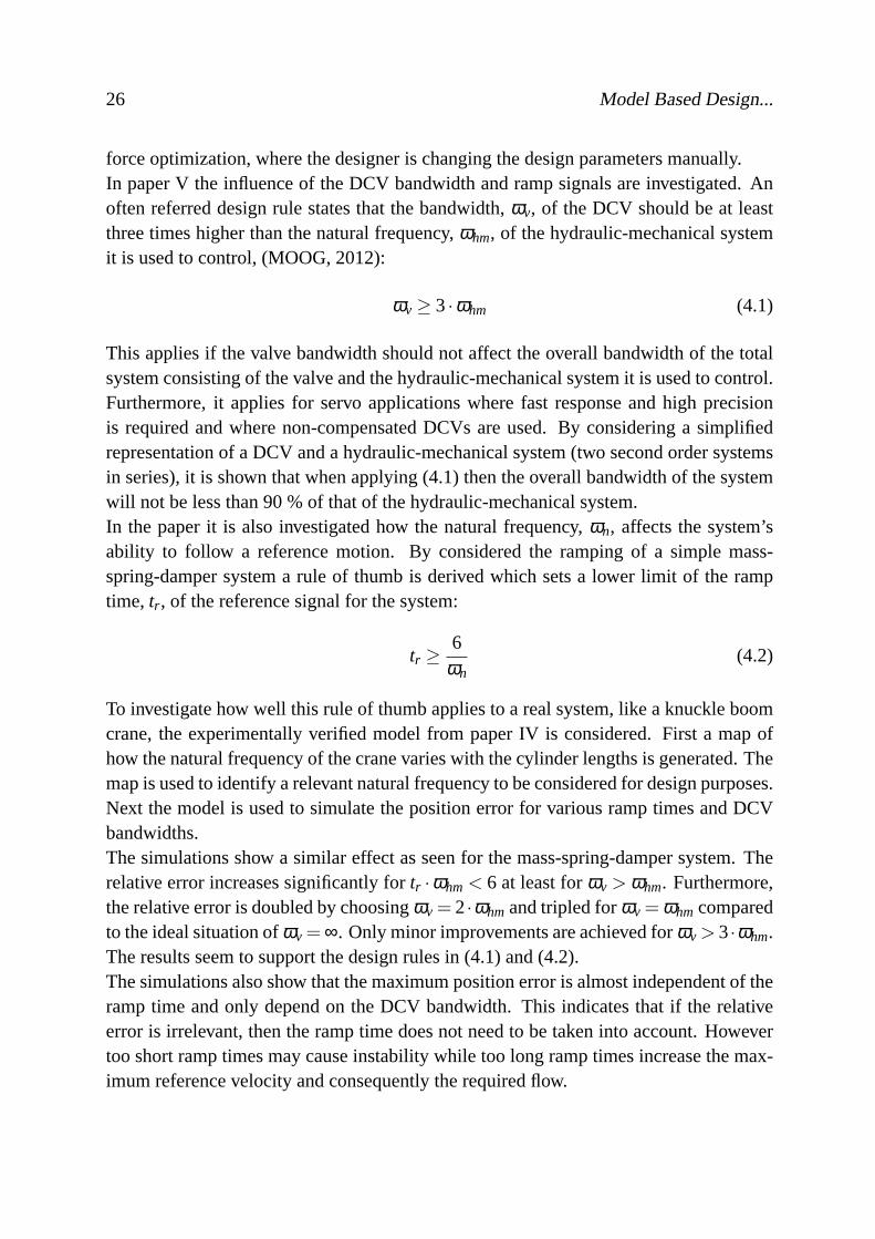
force optimization, where the designer is changing the design parameters manually.In paper V the influence of the DCV bandwidth and ramp signals areinvestigated. Anoften referred design rule states that the bandwidth,ωv, of the DCV should be at leastthree times higher than the natural frequency,ωhm, of the hydraulic-mechanical systemit is used to control, (MOOG, 2012):
ωv ≥ 3 ·ωhm (4.1)
This applies if the valve bandwidth should not affect the overall bandwidth of the totalsystem consisting of the valve and the hydraulic-mechanical system it is used to control.Furthermore, it applies for servo applications where fast response and high precisionis required and where non-compensated DCVs are used. By considering a simplifiedrepresentation of a DCV and a hydraulic-mechanical system (two second order systemsin series), it is shown that when applying (4.1) then the overall bandwidth of the systemwill not be less than 90 % of that of the hydraulic-mechanical system.In the paper it is also investigated how the natural frequency, ωn, affects the system’sability to follow a reference motion. By considered the ramping of a simple mass-spring-damper system a rule of thumb is derived which sets a lower limit of the ramptime, tr , of the reference signal for the system:
tr ≥6
ωn(4.2)
To investigate how well this rule of thumb applies to a real system, like a knuckle boomcrane, the experimentally verified model from paper IV is considered. First a map ofhow the natural frequency of the crane varies with the cylinder lengths is generated. Themap is used to identify a relevant natural frequency to be considered for design purposes.Next the model is used to simulate the position error for various ramp times and DCVbandwidths.The simulations show a similar effect as seen for the mass-spring-damper system. Therelative error increases significantly fortr ·ωhm< 6 at least forωv > ωhm. Furthermore,the relative error is doubled by choosingωv = 2·ωhm and tripled forωv = ωhm comparedto the ideal situation ofωv =∞. Only minor improvements are achieved forωv > 3·ωhm.The results seem to support the design rules in (4.1) and (4.2).The simulations also show that the maximum position error isalmost independent of theramp time and only depend on the DCV bandwidth. This indicates that if the relativeerror is irrelevant, then the ramp time does not need to be taken into account. Howevertoo short ramp times may cause instability while too long ramptimes increase the max-imum reference velocity and consequently the required flow.

Design and Optimization 27
The simulation results confirm the validity of (4.1) and (4.2) and usefulness as generaldesign rules. However, the selection of these design parameters always depend on theacceptable error level for the application to be controlledand for offshore knuckle boomcrane the investigated design rules may be too conservative. A prerequisite to evaluatethis is to have a simulation model, like the one described in paper IV.

28 Model Based Design...

Chapter 5Conclusions
In this dissertation methods for modeling, parameter identification, design and optimiza-tion of a selected piece of offshore pipe handling equipment, a knuckle boom crane, havebeen put forward. Most of the modeling methods are general and can be used for othertypes of hydraulically actuated cranes. Some of the design methods are also general andcan be used for many types of electro-hydraulic motion control systems. A part of thedesign methods, though, are specifically targeting offshore knuckle boom cranes and arenot suited for other cranes like onshore cranes, simply because design requirements aredifferent.The presented methods are developed to accommodate the needs of the system designer.They take into account the challenges encountered by the system designer such as lim-ited access to component data and time available for model development by applying alevel of modeling detail that is suited for system design.
5.1 Contributions
The main challenge of modeling mechanical systems like a knuckle boom crane is toinclude the structural flexibility in an appropriate way. Inpaper I the finite segmentmethod (FSM) is used to model a single crane boom. The finite segment (FS) model iscompared to a finite element (FE) model and very good conformityfor both static anddynamic behavior is achieved. Even though FSM does not represent state of the art offlexibility modeling, this paper shows that FSM is both efficient and sufficient for mod-eling for system design.This is confirmed in paper IV where FSM is used to model structural flexibility anddamping of a complete knuckle boom crane and experimentallyobtained results are usedto calibrate and verify the model. In the paper, approaches for approximation of flexibil-ity and damping parameters are also presented. However, theseparameters usually have
29

30 Model Based Design...
to be experimentally verified and, as it is shown in the paper, it is not uncommon that theflexibility parameters must be reduced by a factor of two and vice versa for the dampingparameters. Naturally, the reason for this is the un-modeledflexibility and damping thatis inconvenient or too difficult to introduce separately.For modeling of directional control valves (DCVs) the main challenge is to include asufficiently accurate representation of the valve dynamics. This is often modeled assecond order system, as it is in paper II. However, for many valves, like pressure com-pensated DCVs, information about dynamic performance is not available and have tobe experimentally determined. In paper II an approach for frequency response testing ispresented and it is shown that a second order system is only able to describe the valvedynamics up to and around the bandwidth of the valve. However, thisis sufficient forsystem design purposes.For pressure compensated DCVs another challenge is the modeling of the pressure com-pensator. In paper II one suggestion is given and in papers III and IV an alternativemodel is used. The alternative model include less parameters and is less computationaldemanding. This is an example of always looking for a best practice within modelingfor system design.With respect to modeling, as well as system design, counterbalance valves (CBVs) aresome of the most difficult components to handle. In some cases they can be modeledwith rather simple semi-physical approaches, but often thisleads to a number of chal-lenges, e.g., related to friction and resulting hysteresis, nonlinear discharge area charac-teristics, varying discharge coefficients and varying flow forces. In those cases the onlyoption may be to use a non-physical (black-box) approach as the one presented in paperIV.Using this black-box model the steady-state behavior of the considered CBV is simu-lated with an accuracy that is not possible to achieve with a semi-physical model. Thedisadvantage of the black-box model is that it relies on several parameters that have tobe experimentally determined. However, sufficiently accurate modeling of CBVs willprobably always require some sort of experimental work. This is also shown in paperIII, where a semi-physical model is used.In general, modeling for system design of a knuckle boom crane, will require experi-mental work for model verification. In paper IV a stepwise approach for calibration andverification of a complete crane model is presented. In each step separate sub-modelsare considered and both optimization techniques and manualtuning is used identify un-certain parameters. This approach may be generalized and used for verification of othertypes of systems as well.In paper III design and optimization of hydraulic systems isdiscussed. It is shown howto arrive at a nominal design with relatively simple steady-state considerations and howsimulation can be used to analyze dynamic system behavior. One of the major challenges

Conclusions 31
with hydraulic systems containing CBVs, is to avoid instability and ensure an acceptablelevel of oscillations during load lowering. A new method for reduction of oscillations isdiscussed and subjected to a design optimization using the Complex method. The newmethod is compared to a more classic method and it is concluded that the new methodis the most suitable for offshore knuckle boom cranes.A central challenge in hydraulic system design is selectionof DCVs and to specify therequired bandwidth of the valve. In paper V simple design rulesfor required DCVbandwidth and minimum ramp times for input signals are presented and discussed. Anexperimentally verified simulation model is used to investigate how these parameters in-fluence both relative and absolute position errors for an electro-hydraulic motion controlsystem.The investigations confirm the validity of these simple design rules. It is also clear thatrequired DCV bandwidth and minimum ramp times always depend onthe acceptableerror level for the specific application. For offshore knuckle boom cranes these designrules may be too conservative, however, a prerequisite for investigating this is to have areliable simulation model.
5.2 Outlook
The main challenge for any model based design approach lies within the ability to pro-duce simulation models that, with a reasonable precision, are able to mimic the behaviorof the real system to be designed. Throughout this dissertation and the appended papersa number of modeling challenges have been addressed. While most of them involveexisting modeling techniques and mainly aim to identify therequired level of modelingdetail, also novel modeling techniques have been presentedlike the black-box model forcounterbalance valves presented in paper IV.The model yield encouraging results in terms of steady-state behavior and it may verywell be used for other types of pressure control valves as well.However, there are stillissues to be investigated in relation to the applied modeling approach. They includephenomena such as dynamic behavior and the influence of hysteresis. This will requiremore experimental work and, in general, an approach for mapping of valve characteris-tics is needed.A major challenge in the offshore industry is that there are very limited opportunities tobuild prototypes for design verification. This of course promotes the use of model baseddesign approaches, although it is difficult to verify modelsbefore any real systems havebeen realized. Even then, it may be difficult to carry out experimental studies requiredfor model verification due to cost and time constraints. Therefore there is a need forprocedures for both model validation and verification which do not require full scale

32 Model Based Design...
experimental work. Such procedures may be based on scale model tests or testing ofindividual components and mapping of their characteristics as it is suggested in paper IIfor directional control valves.Design of hydraulic systems should always be based on sound steady-state considera-tions before attempting to carry out design optimization. Since system design is oftenbased on existing system architectures the remaining part of the job, the component siz-ing/selection, could be automated or standardized by setting up systematic proceduresand using parameterized steady-state models. The use of dynamic simulation modelsfor design optimization could also be automated. However, after the initial design pro-cedure there are often only a few parameters left to be optimized and the potential gainfor automating this procedure is relatively low. The most important value is to have adynamic simulation model that can be used as a design evaluation tool.Introducing new actuation technologies such as separate meter-in separate meter-outcontrol and digital hydraulics represent a higher potential than automated design, be-cause they have the potential to improve or even eliminate problems related to stabilityand efficiency. However, they also represent a higher risk and,once again, the best wayto reduce those risks is to utilize dynamic simulation for design evaluation together withan appropriate amount of testing and model verification.

References 33
References
Alirand, M., Favennec, F., and Lebrun, M. (2002). Pressure components stability analy-sis: A revisited approach.International Journal of Fluid Power, 3(1):33–46.
Andersen, T. O., Hansen, M. R., Pedersen, P., and Conrad, F. (2005). The influence offlow forces on the performance of over center valve systems. In Proceedings of theNinth Scandinavian International Conference on Fluid Power. Linköping, Sweden.
Andersson, J. (2001).Multiobjective optimization in engineering design. Applicationsto fluid power systems. PhD thesis, Linköping University, Linköping, Sweden.
Armstrong-Hélouvry, B., Dupont, P., and de Wit, C. C. (1994). A survey of models,analysis tools and compensation methods for the control of machines with friction.Automatica, 30(7):1083–1138.
Banerjee, A. K. and Nagarajan, S. (1997). Efficient simulation of large overall motionof beams undegoing large deflections.Multibody System Dynamics, 1(1):113–126.
Bauchau, O. A., Epple, A., and Heo, S. (2008). Interpolation if finite rotations in flex-ible multi-body dynamics simulations.Proceedings of the Institution of MechanicalEngineers, Part K: Journal of Multi-body Dynamics, 222(4):353–366.
Bo, L. C. and Pavelescu, D. (1982). The friction-speed relation and its influence on thecritical velocity of stick-slip motion.Wear, 82(3):277–289.
Bonchis, A., Corke, P. I., and Rye, D. C. (1999). A pressure-based, velocity inde-pendent, friction model for asymmetrical hydraulic cylinders. InProceedings of the1999 International Conference on Robotics and Automation, pages 1746–1751. De-troit, Michigan, USA.
Bouzgarrou, B. C., Ray, P., and Gogu, G. (2005). New approach fordynamic modellingof flexible manipulators.Proceedings of the Institution of Mechanical Engineers, PartK: Journal of Multi-body Dynamics, 219(3):285–298.
Box, M. J. (1965). A new method for constrained optimizationand a comparison withother methods.The Computer Journal, 8(1):42–52.
Braccesi, C., Landi, L., and Scaletta, R. (2004). New dual meshless flexible bodymethodology for multi-body dynamics: simulation of generalized moving loads.Pro-ceedings of the Institution of Mechanical Engineers, Part K: Journal of Multi-bodyDynamics, 218(1):51–62.

34 Model Based Design...
Burrows, C. R. (2000). Fluid power systems - some research issues. Proceedings ofthe Institution of Mechanical Engineers, Part C: Journal ofMechanical EngineeringScience, 214(1):203–220.
Chapple, P. J. and Tilley, D. G. (1994). Evaluation techniquesfor the selection of coun-terbalance valves. InProceedings of the Expo and Technical Conference for Electrohy-draulic and Electropneumatic Motion Control Technology, pages 351–359. Anaheim,USA.
Connelly, J. and Huston, R. L. (1994a). The dynamics of flexiblemultibody systems:A finite segment approach — I. Theoretical aspects.Computers and Structures,50(2):255–258.
Connelly, J. and Huston, R. L. (1994b). The dynamics of flexiblemultibody systems:A finite segment approach — II. Example problems.Computers and Structures,50(2):259–262.
da Silva, J. C. (2000). Artificial intelligence enhancing fluid power system design. InProceeding of the 48th National Conference on Fluid Power, pages 157–168. Chicago,Illinois, USA.
da Silva, J. C. and Back, N. (2000). Shaping the process of fluidpower system designapplying an expert system.Research in Enginnering Design, 12(21):8–17.
Darlington, M., Culley, S., and Potter, S. (2001). Knowledge and reasoning issues raisedin automating the conceptual design of fluid power systems.International Journal ofFluid Power, 2(2):75–85.
Dunlop, G. R. and Rayudu, R. K. (1993). An expert assistant for hydraulic systems. InProceedings of the First New Zealand International Two-Stream Conference on Arti-ficial Neural Networks and Expert Systems, pages 314–316. Dunedin, New Zealand.
Eberhard, P. and Schiehlen, W. (2006). Computational dynamics of multibody systems:History, formalisms, and applications.Journal of Computational and Nonlinear Dy-namics, 1(1):3–12.
Engler, F., Baum, H., and von Dombrowski, R. (2010). Developmentenvironment forfluid-power-mechatronic systems. InProceedings of the 7th International Fluid PowerConference. Aachen, Germany.
Eriksson, B. and Palmberg, J.-O. (2011). Individual metering fluid power systems: chal-lenges and opportunities.Proceedings of the Institution of Mechanical Engineers,Part I: Journal of Systems and Control Engineering, 225(2):196–211.

References 35
Gerstmayr, J. and Schöberl, J. (2006). A 3d finite element method for flexible multibodysystems.Multibody System Dynamics, 15(4):309–324.
Gordic, D., Barbic, M., and Jovicic, N. (2004). Modelling of spool position feedbackservovalves.International Journal of Fluid Power, 5(1):37–50.
Hampson, S. P., Brain, C., Tomlinson, S. P., Chawdhry, P. K., Medland, A. J., and Bur-rows, C. R. (1996). System design - improved efficiency through software integration.In Proceedings of the 9th Bath International Fluid Power Workshop. Bath, UK.
Handroos, H., Halme, J., and Vilenius, M. (1993). Steady-stateand dynamic proper-ties of counter balance valves. InProceedings of the 3rd Scandinavian InternationalConference on Fluid Power, pages 215–235. Linköping, Sweden.
Handroos, H. M. and Vilenius, M. J. (1991). Flexible semi-empirical models for hy-draulic flow control valves. volume 113, pages 232–238.
Hansen, M. R. and Andersen, T. (2005). System topology optimization. volume 2, pages133–141.
Hansen, M. R., Andersen, T., and Conrad, F. (2001). Experimentally based analysisand synthesis of hydraulically actuated loader crane. InBath Workshop on PowerTransmission and Motion Control, pages 259–274. Bath, UK.
Hansen, M. R. and Andersen, T. O. (2001). A design procedure for actuator control sys-tem using design optimization. InProceedings of the 7th Scandinavian InternationalConference on Fluid Power. Linköping, Sweden.
Hughes, E. J., Richards, T. G., and Tilley, D. G. (2001). Development of a design supporttool for fluid power system design.Journal of Engineering Design, 12(2):75–92.
Huston, R. L. (1981). Multi-body dynamics including the effects of flexibility and com-pliance.Computers and Structures, 14(5-6):443–451.
Huston, R. L. (1991). Computer methods in flexible multibody dynamics.InternationalJournal for Numerical Methods in Engineering, 32(8):1657–1668.
Huston, R. L. and Wang, Y. (1993). Flexibility effects in multibody systems. InCom-puter Aided Analysis of Rigid and Flexible Mechanical Systems: Proceedings of theNATO Advanced Study Institute, pages 351–376. Troia, Portugal.
Käppi, T. and Ellman, A. (1999). Modelling and simulation of proportional mobilevalves. InProceedings of the 4th JHPS International Symposium on Fluid Power,pages 531–536. Tokyo, Japan.

36 Model Based Design...
Käppi, T. and Ellman, A. (2000). Analytical methods for definingpressure compensatordynamics.Fluid Power Systems and Technology, 7:121–125.
Krimbacher, N., Garstenauer, M., and Scheidl, R. (2001). Optimization of hydraulic sys-tems by means of numerical simulation. InProceedings of the 2nd International Work-shop on Computer Software for Design, pages 76–83. Ostrava-Malenovice, CzechRepublic.
Krus, P., Jansson, A., and Palmberg, J.-O. (1991). Optimizationfor component selec-tion in hydraulic systems. InProceedings of the 4th Bath International Fluid PowerWorkshop, pages 219–231. Bath, UK.
Liermann, M. and Murrenhoff, H. (2005). Knowledge based tools for the design ofservo-hydraulic closed loop control.Power Transmission and Control, pages 17–28.
Lin, Z.-C. and Shen, C.-C. (1995). An investigation of an expert system for hydrauliccircuit design with learning.Artificial Intelligence in Engineering, 9(3):153–165.
Linjama, M. and Vilenius, M. (2007). Digital hydraulics - towards the perfect valvetechnology. InProceedings of the Tenth Scandinavian International Conference onFluid Power. Tampere, Finland.
Lisowski, E. and Stecki, J. S. (1999). Stability of a hydraulic counterbalancing system ofhydraulic winch. InProceedings of the Sixth Scandinavian International Conferenceon Fluid Power, pages 921–933. Tampere, Finland.
Maré, J.-C. (2012). Friction modelling and simulation at system level: a practical viewfor the designer.Proceedings of the Institution of Mechanical Engineers, Part I: Jour-nal of Systems and Control Engineering, 226(6):728–741.
Maré, J.-C. and Attar, B. (2008). Enhanced model of four way valves characteristics andits validation at low temperature.International Journal of Fluid Power, 9(3):35–43.
Merritt, H. E. (1967).Hydraulic control systems. Wiley.
Michel, S. and Weber, J. (2012). Electrohydraulic compact-drives for low power appli-cations considering energy-efficiency anf high inertial loads. InProceedings of the7th FPNI PhD Symposium on Fluid Power, pages 869–888. Reggio Emilia, Italy.
Miyakawa, S. (1978). Stability of a hydraulic circuit with a counterbalance valve.Bul-letin of the JSME, 21(162):1750–1756.
MOOG (2012). Electrohydraulic valves... a technical look. Technical report, Moog Inc.http://www.moog.com/literature/ICD/Valves-Introduction.pdf.

References 37
Mostofi, A. (1999). The incorporation of damping in lumped-parameter modelling tech-niques. Proceedings of the Institution of Mechanical Engineers, Part K: Journal ofMulti-body Dynamics, 213(1):11–17.
Márton, L., Fodor, S., and Sepehri, N. (2011). A practical method for friction identifi-cation in hydraulic actuators.Mechatronics, 21(1):350–356.
Muller, M. T. and Fales, R. C. (2008). Design and analysis of a two-stage poppet valvefor flow control. International Journal of Fluid Power, 9(1):17–26.
Munteanu, M. G., Gogu, R., and Ray, P. (2006). Fast and simple dynamic analysis offlexible multi-body systems.Proceedings of the Institution of Mechanical Engineers,Part K: Journal of Multi-body Dynamics, 220(4):219–237.
Naets, F., Tamarozzi, T., Heirman, G. H. K., and Desmet, W. (2012). Real-time flexiblemultibody simulation with global model parameterization.Multibody System Dynam-ics, 27(3):267–284.
Nielsen, B., Entwistle, R. T., Tandrup, L. B., and Andersen, T. O.(2006). Parameteriseddynamic model of a 4-way spool valve - an experimental study.
Nikravesh, P. E. (1988).Computer-aided analysis of mechanical systems. Prentice Hall.
Olsson, H., Åström, K. J., Canudas de Wit, C., Gäfvert, M., and Lischinsky, P. (1998).Friction models and friction compensation.Europena Journal of Control, 4(3):176–195.
Opdenbosch, P., Sadegh, N., Book, W., Murray, T., and Yang, R. (2009). Modelling anelectro-hydraulic poppet valve.International Journal of Fluid Power, 10(1):7–15.
Ottestad, M., Nilsen, N., and Hansen, M. R. (2012). Reducing the static friction inhydraulic cylinders by maintaining relative velocity between piston and cylinder. InProceedings of the 12th International Conference on Control, Automation and Sys-tems, pages 764–769. Jeju Island, Korea.
Overdiek, G. (1981). Design and characteristics of hydraulic winch controls by coun-terbalance valves. InProceedings of the European Conference on Hydrostatic Trans-mission for Vehicle Applications. Achen, Germany.
Palmberg, J.-O. (1995). Design of fluid-mechanical systems - methods and tools to meetfuture needs. InProceedings of Hydraulikdagar i Linköping. Linköping, Sweden.
Papadopoulos, E. and Davliakos, I. (2004). A systematic methodology for optimalcomponent selection of electrohydralic servosystems.International Journal of FluidPower, 5(3):15–24.

38 Model Based Design...
Pascal, M. (2001). Some open problems in dynamic analysis offlexible multibodysystems.Multibody System Dynamics, 5(4):315–334.
Pedersen, H. C. (2004). Power management in mobile hydraulic applications - an ap-proach for designing hydraulic power supply systems. InProceedings of the 3rd FPNIPhD Symposium on Fluid Power, pages 125–139. Terrassa, Spain.
Persson, T., Krus, P., and Palmberg, J.-O. (1989). The dynamicproperties of over-centervalves in mobile systems. InProceedings of the 2nd International Conference onFluid Power Transmission and Control. Hangzhou, China.
Rahman, M. M., Porteiro, J. L. F., and Weber, S. T. (1997). Numerical solution andanimation of oscillating turbulent flow in a counterbalancevalves. InProceedingsof the Thirty-Second Intersociety Energy Conversion Engineering Conference. Hon-olulu, Hawaii, USA.
Raman-Nair, W. and Baddour, R. E. (2003). Three-dimensionaldynamics of a flexi-ble marine riser undergoing large elastic deformations.Multibody System Dynamics,10(4):393–423.
Ramli, Y., Chapple, P. J., and Tilley, D. G. (1995). Applicationof computer aideddesign (cad) in hydraulic systems using counterbalance valves. InProceedings of the4th International Conference on Computer-Aided Design and Computer Graphics.Wuhan, China.
Ruan, J., Burton, R., Ukrainetz, P., and Xu, Y. M. (2001). Two-dimensional pressurecontrol valve.Proceedings of the Institution of Mechanical Engineers, Part C: Journalof Mechanical Engineering Science, 215(9):1031–1039.
Schiehlen, W. (1997). Multibody system dynamics: Roots andperspectives.MultibodySystem Dynamics, 1(2):149–188.
Schiehlen, W. (2007). Research trends in multibody systemsdynamics. MultibodySystem Dynamics, 18(1):3–13.
Schlemmer, K. and Murrenhoff, H. (2008). Development of an expert system for electro-hydraulic motion control design. InThe 20th International Conference on Hydraulicsand Pneumatics, pages 259–268. Prague, Czech Republic.
Shabana, A. A. (1997). Flexible multibody dynamics: Review ofpast and recent devel-opments.Multibody System Dynamics, 1(2):189–222.
Stecki, J. S. and Garbacik, A. (2002). Fluid Power Net Publications.

References 39
Steiner, B. and Scheidl, R. (2005). A computer aided conceptual design method forhydraulic components.Power Transmission and Control, pages 209–221.
Tran, X. B., Hafizah, N., and Yanada, H. (2012). modeling of dynamicfriction behaviorsof hydraulic cylinders.Mechatronics, 22(1):65–75.
Tørdal, S. S. and Klausen, A. (2013). Dynamiske karakteristikker av Brevini HPV41med åpen og lukket sløyferegulering. Bachelor’s thesis, University of Agder, Grim-stad, Norway.In Norwegian.
Yanada, H. and Sekikawa, Y. (2008). Modeling of dynamic behaviors of friction.Mecha-tronics, 18(7):330–339.
Yoo, W.-S., Kim, K.-N., Kim, H.-W., and Sohn, J.-H. (2007). Developments of multi-body systems dynamics: Computer simulations and experiments. Multibody SystemDynamics, 18(1):35–58.
Zähe, B. (1995). Stability of load holding circuits with counterbalance valves. InPro-ceedings of the 8th Bath International Fluid Power Workshop, pages 60–75. Bath,UK.
Zhang, R., Alleyne, A. G., and Prasetiawan, E. A. (2002). Performance limitations of aclass of two-stage electro-hydraulic flow valves.International Journal of Fluid Power,3(1):47–53.

40 Paper I

Paper IA Method for Finite Element Based
Modeling of Flexible Components in
Time Domain Simulation of Knuckle Boom
Crane
Jan Henriksen,Morten Kollerup Bak and Michael Rygaard Hansen
41

42 Paper I
This paper has been published as:
J. Henriksen, M. K. Bak and M. R. Hansen, “A Method for Finite Element Based Mod-eling of Flexible Components in Time Domain Simulation of Knuckle Boom Crane”,The 24th International Congress on Condition Monitoring and Diagnostics Engineer-ing Management, pp. 1215-1224. Stavanger, Norway, May 30 - June 1, 2011.

A Method for Finite Element Based Modeling of Flexible Components... 43
A Method for Finite Element Based Modeling of Flexible
Components in Time Domain Simulation of Knuckle Boom
Crane
Jan Henriksen, Morten Kollerup Bak and Michael Rygaard HansenDepartment of Engineering Sciences
Faculty of Engineering and Science, University of AgderJon Lilletunsvei 9, 4879 Grimstad, Norway
Abstract — In this paper emphasis is on modeling of the flexibility of the different mainstructural components of an offshore knuckle boom crane. The modeling approach usesresults from finite element analysis of the structural components to calibrate a multi-body dynamic model of the crane. The calibration is a parameter identification thatminimizes the deviation between the static and dynamic behavior of the finite elementmodel of the beam-like jibs of the crane with that of lumped beam models. The latterapproach allows for an efficient simulation of tool point control schemes that takes intoaccount all important structural deflections and vibrations.
Keywords — Hydraulic crane, multi-body system mechanics, lumped beammodel.
44 Paper I
1 Introduction
The ongoing competition between manufacturers of hydraulically actuated offshore equip-ment continuously sets new references for main performanceparameters such as price,payload and reach, controllability, weight, efficiency and reliability. Since developmenttime and costs must be kept at a minimum this leaves the designengineer in a challengedposition typically facing a complex task of a strongly dynamic and multidisciplinary na-ture. As already pointed out in Palmberg (1995) computer based time domain simulationand optimization techniques are potentially excellent tools for the challenged designerin the iterative design phase. Another important parameter concerning said equipment ismodel based condition based maintenance (CBM). The aim of this work is to investigatethe possibilities of using time domain simulation on the hydraulic-mechanical system ofhydraulically actuated cranes with a view to obtain computational efficient models thatare sufficiently precise to be used both online but also as a diagnostics tool in CBM.There are many factors that influence the performance of hydraulic cranes. The mechan-ical structure of a boom causes gravitational and inertia loads. Friction forces may alsobe significant, especially in a telescopic manipulator. A hydraulic crane uses full strokecontrol and is subjected to hard non-linearities, time varying parameters, external dis-turbances, a number of saturation phenomena and coupling effects and even though thehydraulic system in principle is quite simple, dynamic problems may appear in practice.To avoid cavitation and for safety reasons, often the most practical way is to use coun-terbalance valves. The influence of load pressure variations on the velocity of the actu-ators may be eliminated in several ways, Andersen and Hansen (2001), but the simplestmethod is to apply a pressure compensated proportional valve. However, the combina-tion of these two hydraulic valves will often decrease the stability margin significantly.Hence, a certain pressure feedback/load dependancy or otherdesign manipulations ofthe individual hydraulic circuits are often introduced/accepted in one or more of themain cylinder functions. In terms of kinematic structure, the hydraulic cranes can betreated as mechanisms made of several stiff and flexible links connected with revolutejoints. From the point of view of topology, the manipulator is globally an open kine-matic chain, with locally closed kinematic chains from the steering and control systemsin the shape of cylinders and dyad links. Closed loop controlof pipe handler cranes israpidly developing. Position and pressure transducers aregenerally accepted and fullyintegrated in tool point control.An important question is whether models with an acceptable and useful accuracy maybe established without excessive testing and tuning of simulation parameters. Previouswork, Mikkola and Handroos (1996) and Ellman et al. (1996), has shown very encour-aging accuracy of models on hydraulic driven boom mechanisms. There are severalparameters associated with the modeling of an entire hydraulic crane that are difficult to

A Method for Finite Element Based Modeling of Flexible Components... 45
estimate and measure, see for example Ebbesen and Hansen (2010) and Pedersen et al.(2010). They include damping, friction, flexibility and backlash in both the hydraulicand mechanical components. In this paper the importance of including the flexibilityof the structural parts are investigated and an approach to the flexibility modeling ofthe beam-like arms that are present in any hydraulic crane isput forward. A so-calledknuckle boom crane used for pipe handling is used to exemplify the approach. For sucha crane there might be different failure mechanisms both related to the hydraulics andthe mechanics. The dynamic response of the crane booms duringoperation can be asignificant indicator of a number of wear and fatigue phenomena.
2 Considered System
Knuckle boom cranes are used for a wide range of offshore and marine operations andtherefore exist in different variations. The considered crane is used on a drilling rig forhandling of the drill pipes.Considering the crane as a general mechatronic system, three different sub-systems canbe identified:
1. A mechanical system providing the geometric and load carrying properties.
2. A primarily hydraulic actuation system driving the mechanical system.
3. An electronic control system for control of the crane through the actuation system.
The main components of the mechanical system are a rotating part mounted on a pedestalwith a slewing bearing in between, an inner jib, an outer jib and agripping yoke for thepipe handling. See Fig. 1.
Pipe Deck
Pedestal
Rotating Part
Inner Jib
Outer Jib
Gripping Yoke
Slewing Bearing
23.5m
16m
Figure 1: Main components of the cranes mechanical system.

46 Paper I
The hydraulic system consists of three primary circuits for:
1. Tilting of the inner jib.
2. Tilting of the outer jib.
3. Slewing of the crane.
Furthermore it contains some secondary circuits for opening and closing etc. of thegripping yoke, which are not considered here. A total model ofthe crane is describedin detail in Bak et al. (2011). In the following the modeling ofthe outer jib is givenspecial attention since it qualifies as a structural component where the flexibility shouldbe taken into account.
3 Modeling of the Outer Jib Flexibility
The outer jib is a beam-like structure, see Fig. 2, that is kinematically connected to theinner jib via a revolute joint, point A. The rotation around theaxis of the revolute jointis controlled by means of two double acting hydraulic cylinders in parallel that connectto the outer jib in a spherical joint, point B. The axis of the revolute joint correspondsto the y-axis of the local coordinate system attached to the outer jib, see Figure 2. Thegripping yoke is connected to the outer jib via a hydraulically damped universal joint atthe tip of the outer jib, point C.The shape of the jib roughly reflects the bending moment in thestructure and increasesin cross section dimensions from the revolute joint to the cross section at the cylinderconnection. Thereafter, the cross section gradually decreases in size until the end of thejib where the gripping yoke connection is attached. Seen froma solid mechanics pointof view the outer jib may be thought of as a beam that is hinged inpoint A and simplysupported in point B when considered in the xz-plane, and as a cantilever beam fixed inpoint A when considered in the xy-plane.
3.1 Finite Element Model
Finite element analysis is a widely accepted method for linear deflections, stress, strainsand vibrational analysis of structural parts. This method has been used to generate aprecise picture of the flexibility of the outer jib and to act as foundation for the calibrationof a more simple lumped multi-body model.The finite element analysis comprises different linear analyses of the outer jib. Theouter jib is modeled as a plate structure with cross sectionalreinforcements at differentintervals. The physical model is built up by plates with different thickness, however,
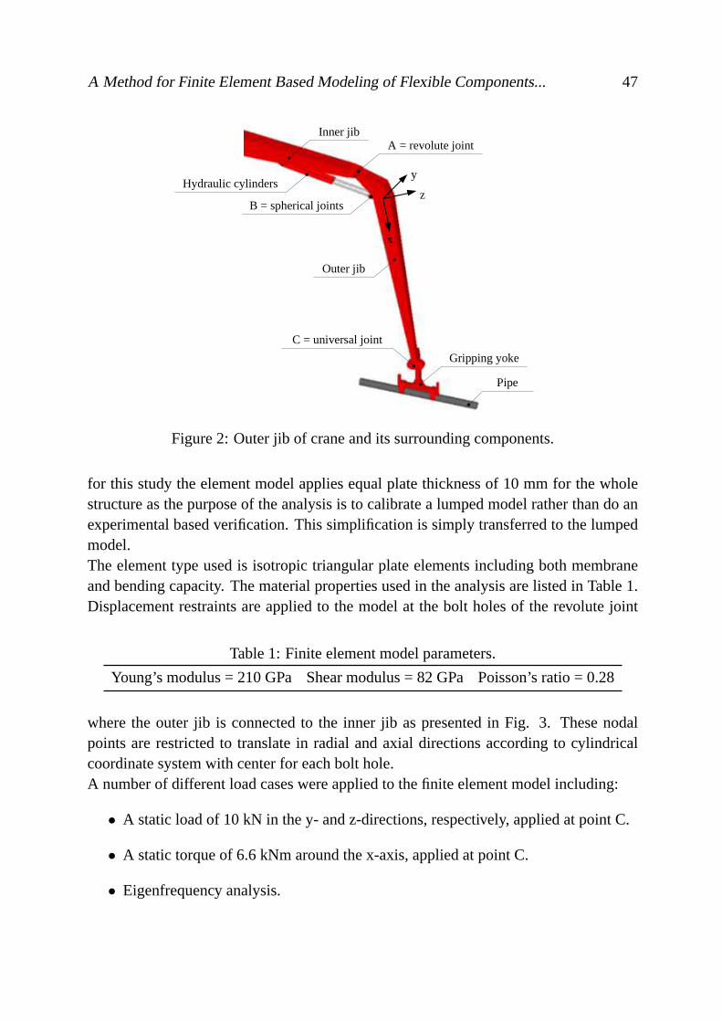
A Method for Finite Element Based Modeling of Flexible Components... 47
A = revolute jointInner jib
Hydraulic cylinders
B = spherical joints
Outer jib
C = universal joint
Gripping yoke
Pipe
x
y
z
Figure 2: Outer jib of crane and its surrounding components.
for this study the element model applies equal plate thickness of 10 mm for the wholestructure as the purpose of the analysis is to calibrate a lumped model rather than do anexperimental based verification. This simplification is simply transferred to the lumpedmodel.The element type used is isotropic triangular plate elements including both membraneand bending capacity. The material properties used in the analysis are listed in Table 1.Displacement restraints are applied to the model at the bolt holes of the revolute joint
Table 1: Finite element model parameters.
Young’s modulus = 210 GPa Shear modulus = 82 GPa Poisson’s ratio = 0.28
where the outer jib is connected to the inner jib as presented in Fig. 3. These nodalpoints are restricted to translate in radial and axial directions according to cylindricalcoordinate system with center for each bolt hole.A number of different load cases were applied to the finite element model including:
• A static load of 10 kN in the y- and z-directions, respectively, applied at point C.
• A static torque of 6.6 kNm around the x-axis, applied at point C.
• Eigenfrequency analysis.

48 Paper I
A
B
C
x
z
y
Figure 3: Boundary conditions applied to outer jib.
3.2 Lumped Model
In a lumped model the mechanical system is modeled as a chain of 3D-rigid segmentskinematically attached to each other by means of kinematic joints. The main advantagesof lumping a beam in a multibody simulation model are:
• Simple model development from cross sectional data.
• Possible to use standard joints and rigid bodies available in libraries.
• Possible to apply external loading anywhere on the beam like component via therigid bodies.
• Possible to discard unwanted degrees of freedom.
The individual segments are modeled as rigid bodies with rotational springs that may beattached to the two neighboring bodies. The original work within this area was carriedout by Kane et al. (1987) and Huston and Wang (1993).For bending the segment stiffness is:
kS=2 ·E · I
L(1)

A Method for Finite Element Based Modeling of Flexible Components... 49
Where E is the Young’s modulus, I is the area moment of inertiaand L is the length ofthe segment.For torsion the segment stiffness is:
kS=2 ·G · Ip
L(2)
Where G is the shear modulus, Ip is the polar moment of inertiaand L is the length ofthe segment.If two segments are connected, then the resulting connecting stiffness is:
kC =1
1kS,1
+ 1kS,2
(3)
Where kS,1 is the stiffness of the first segment and kS,2 is thestiffness of the secondsegment of the connection.If the segment is the first or last segment of the beam then, depending on the physicalconnection between the beam and its surroundings, the rotational springs may either beconnected to a fixed interface or to nothing yielding the following possible connectionstiffnesses at the beam ends:
kC = kS f ixed
kC = 0 f ree(4)
In the current work the kinematical connections between the segments discard the po-sitional degrees of freedom thereby avoiding a stiff model.Also, the force from thehydraulic cylinder (point B) is easily applied to the third segment as an exterior force.The segmentation is shown in Fig. 4.The outer jib has been divided into nine segments but this number can be reduced formost practical problems. The topology of the segmentation is listed and in Table 2.The segments have tapered rectangular hollow cross sections. For simplicity an average
Table 2: Topology of segmentation of outer jib.
OJ segment Previous body Next body Previous joint Next joint
S1 Last IJ segment S2 Revolute joint Spherical jointSi, i = 1...8 Si −1 Si +1 Spherical joint Spherical jointS9 S8 Gripping yoke Spherical joint Revolute joint
value of the stiffnesses of the segments was used, so that each segment had a singlevalue for each of its three stiffnesses. In Table 3 the different segment and connectionstiffnesses are listed.

50 Paper I
A
B
C
S1S2
S3
S4
x
z
y
S5
S6
S7
S8
S9
Figure 4: Segmentation of outer jib. The local coordinate system of segment 5 (S5) isshown.
Table 3: Stiffnesses [MNn/rad] of outer jib segmentation fornominal lumped model.
No. l [m] kSx kSy kSz kprevC,x knext
Cx kprevCy knext
Cy kprevCz knext
Cz
S1 0.7 2300 3100 2940 2300834
01280
2940879S2 2.05 1310 2180 1250
975 1670 877S3 1.045 3830 7140 2910984 1820 765S4 2.5 1330 2440 1040
551 886 530S5 2.5 943 1390 1080 363 613 318S6 2.5 590 1100 450 229 442 177S7 2.5 374 687 292 80 139 71S8 4.653 102 174 93 65 109 61S9 1.4 179 294 177 179 0 0
3.3 Comparison and Calibration
In the following the main results from the finite element modeland the lumped modelare compared. Two different lumped models are displayed, the nominal that is deriveddirectly from cross sectional data, see Table 3, and a calibrated model that is tuned sothat the two fundamental eigenfrequencies correspond to that of the finite element model.The calibration has been performed by simply scaling the segment rotational stiffnesses

A Method for Finite Element Based Modeling of Flexible Components... 51
with the same scaling factor. Hence, only two calibration parameters were introduced:
k∗Sx,i = kSx,i
k∗Sy,i = 1.05·kSy,i
k∗Sz,i = 0.96·kSz,i
(5)
Wherei = 1...9 and * indicates the calibrated model.In Fig. 5 the deflections of what approximates the neutral axisof the beam are shownfor the 10 kN static load cases.Further, in Table 4 the two lowest eigenfrequencies of the model are listed. The cor-responding eigenmodes are the fundamental bending mode in the xy-plane and the xz-plane, respectively.The non-calibrated model has some deviations from the finiteelement model, however,they would be acceptable for most engineering purposes. With a relatively simple cal-ibration it is possible to adjust the fundamental eigenfrequencies quite close to that ofthe finite element model. The deflection curves show a more pronounced deviation, es-pecially in the out-of-plane direction, i.e., in the xy-plane. Since the effect of addingthe flexibility of beams in simulation of hydraulic cranes isexpected to have most sig-nificant impact on dynamic results the main target of the calibration has been to fit theeigenfrequencies and the static deflections have been considered secondary because theyfit quite well. If the static deflections had shown a larger deviation from the finite ele-ment model, the calibration might need to be carried out as a multi-criteria optimizationwhere both deviations from eigenfrequencies as well as staticdeflections are minimizedsimultaneously.
Table 4: Eigenfrequencies of the different models.
Model fxy [Hz] fxz [Hz]
Finite element 3.21 5.40Lumped (nom.) 3.26 5.29Lumped (cal.) 3.21 5.40
4 Simulation Results
In this section the importance of adding flexibility of cranejibs are shown by using thecalibrated lumped model in a time domain simulation model that includes the hydrauliccircuit that control the motion of the outer jib relative to that of the inner jib and comparethe results with those obtained using a rigid body model.

52 Paper I
0 50 1000
2
4
6
8
10
12
x (B − C) [%]
u z [mm
]
FEMLumped (cal.)Lumped (nom.)
0 50 1000
5
10
15
20
25
30
x (B − C) [%]u y [m
m]
FEMLumped (cal.)Lumped (nom.)
Figure 5: Deflections of outer jib neutral axis versus percentage distance from B to Cfor 10 kN loads in y- and z-directions.
4.1 Hydraulic Circuit
The hydraulic circuit, Fig. 6, consists of a pressure compensated proportional directionalvalve, counterbalance valves for controlled load lowering and two cylinders.The control valve consist of a 4/3 proportional directionalvalve and a pressure reducingvalve representing the pressure compensator. A small volume is added between the twovalves to avoid algebraic loops. The circuit which directs the load sensing pressure tothe spring side of pressure compensator is modeled as a pressure source and a functionblock which sets the value of the pressure source equal to the highest value of the 4/3valve’s A- and B-port pressures. This does not represent the actual functionality of theload sensing circuit, but since the load sensing pressure always is the highest of the A-and B-port pressures the result is the same and it simplifies the model.The control signal for the valve is modeled as a normalized signal which can be variedcontinuously between 1- and 1 and thereby controlling both flow rate and direction ofthe hydraulic fluid through the control valve. It is represented by a signal block whichallows specifying the control signal as a function of the simulation time.Each counterbalances valve consists of a check valve for free flow into the actuator anda pilot operated check valve which opens at a certain crackingpressure, in this case 220bar, for flow out of the actuator. The cracking pressure indicates the value at which thevalve’s A-port pressure is able to open the valve itself. The valve therefore also serves asboth shock- and relief valves with setting of 220 bar. For the main function the openingof the valve is assisted by the pilot pressure, i.e., the pressure of the opposite side of the

A Method for Finite Element Based Modeling of Flexible Components... 53
Figure 6: Model structure of hydraulic circuit for tilting of outer jib.
actuator to which the counterbalance valve is connected. Thepilot pressure lowers theeffective setting of the valve by a factor determined by the pilot ratio, which is 3:1 forboth counterbalance valves.
4.2 Simulation Sequence
To demonstrate the importance of including the flexibility in models of multi-body sys-tems, a simulation is carried out for both a rigid body model and a flexible model. Thesequence of the simulation is illustrated in Fig. 7 and is modeled by prescribing thenormalized input signal to the directional control valve asa time series. The hydrauliccylinder is retracted for the first 11 seconds, then held fixedfor 5 seconds before it is ex-tended to its initial position in 19 seconds. The extra time used for extending is becauseof the differential area of the cylinder yielding two different gearings between valve flowand cylinder speed. The simulation model is developed and executed using the commer-cial simulation software SimulationXR©.The behavior of the system changed significantly when replacing the lumped model witha single rigid body representing the entire outer jib. In Fig. 8 the cylinder force is shownfor both cases.Obviously, the rigid body model predicts instability in the system during cylinder extrac-tion. The steady state values are the same for the two simulation models but the dynamicresults and derived values such as vibration level, fatigueetc. are totally different.

54 Paper I
t = 0 s t = 11...16 s t = 35 s
Figure 7: Model structure of hydraulic circuit for tilting of outer jib.
0 5 10 15 20 25 30 35−1000
−500
0
500
1000
1500
t [s]
F cyl [k
N]
Flexible (lumped)Rigid
Figure 8: Variation in cylinder force.
5 Conclusions
In this paper the modeling of flexible hydraulically actuated cranes has been investi-gated. Emphasis has been on the modeling of the structural flexibility of the outer jibof a knuckle boom crane used for pipe handling in offshore applications. An approachusing segments to a 3D lumped model is put forward. A finite element model has beendeveloped and used to evaluate and calibrate the lumped model. Comparison betweenthe finite element model and the lumped model show that a rather rough approximationof the bending stiffness of the segments of the lumped model yields quite satisfactory re-sults both regarding dynamic and static behavior. Also, two simple one-dimensional cal-ibrations within a few percentages of the nominal model yields a behavior of the lumpedmodel that for most engineering applications corresponds to that of the finite element
A Method for Finite Element Based Modeling of Flexible Components... 55
model. From a CBM point of view the lumped model seems to be well suited for bothdiagnostics capable of analyzing large time series with a relatively low computationaleffort. Further, the importance of including flexibility inthe modeling of hydraulicallyactuated cranes is clearly demonstrated on the investigated knuckle boom crane. A sim-ulation model that take into account the hydraulic circuit and the cylinders that controlthe outer jib produce totally different dynamic behavior depending on whether the outerjib is modeled as a single rigid body or as the calibrated lumped model.
Acknowledgment
The work presented in this paper is funded by the Norwegian Ministry of Education andResearch and Aker Solutions.
References
Andersen, T. O. and Hansen, M. R. (2001). Evaluation of velocity control conceptsinvolving counter balance valves in mobile cranes. InProceedings of the 5th Interna-tional Conference on Fluid Power Transmission and Control. Hangzhou, China.
Bak, M. K., Hansen, M. R., and Nordhammer, P. A. (2011). Virtual prototyping - modelof offshore knuckle boom crane. InProceedings of the 24th International Congress onCondition Monitoring and Diagnostics Engineering Management, pages 1242–1252.Stavanger, Norway.
Ebbesen, M. K. and Hansen, M. R. (2010). Correction scheme for tool point velocitycontrol of a flexible hydraulically actuated manipulator. In Proceedings of the IASTED29th International Conference on Modeling, Identificationand Control. Innsbruck,Austria.
Ellman, A., Käppi, T., and Vilenius, M. J. (1996). Simulation and analysis of hydrauli-cally driven boom mechanisms. InProceedings of the 9th Bath International FluidPower Workshop, pages 413–429. Bath, UK.
Huston, R. L. and Wang, Y. (1993). Flexibility effects in multibody systems. InCom-puter Aided Analysis of Rigid and Flexible Mechanical Systems: Proceedings of theNATO Advanced Study Institute, pages 351–376. Troia, Portugal.
Kane, T. R., Ryan, R. R., and Banerjee, A. K. (1987). Dynamics of a cantilever beamattached to a moving base.Journal of Guidance, Control and Dynamics, 10(2):139–151.

56 Paper I
Mikkola, A. and Handroos, H. (1996). Modeling and simulation ofa flexible hydraulic-driven log crane. InProceedings of the 9th Bath International Fluid Power Workshop.Bath, UK.
Palmberg, J.-O. (1995). Design of fluid-mechanical systems - methods and tools to meetfuture needs. InProceedings of Hydraulikdagar i Linköping. Linköping, Sweden.
Pedersen, M. M., Hansen, M. R., and Ballebye, M. (2010). Developing a tool pointcontrol scheme for a hydraulic crane using interactive real-time dynamic simulation.Modeling, Identification and Control, 31(4):133–143.
Paper IIModeling, Performance Testing and
Parameter Identification of
Pressure Compensated Proportional
Directional Control Valves
Morten Kollerup Bak and Michael Rygaard Hansen
57

58 Paper II
This paper has been published as:
M. K. Bak and M. R. Hansen, “Modeling, Performance Testing and Parameter Iden-tification of Pressure Compensated Proportional Directional Control Valves” The 7thFPNI PhD Symposium on Fluid Power, pp. 889-908. Reggio Emilia, Italy, June 27 - 30,2012.

Modeling, Performance Testing and Parameter Identification... 59
Modeling, Performance Testing and Parameter Identification
of Pressure Compensated Proportional Directional Control
Valves
Morten Kollerup Bak and Michael Rygaard HansenDepartment of Engineering Sciences
Faculty of Engineering and Science, University of AgderJon Lilletunsvei 9, 4879 Grimstad, Norway
Abstract — This paper presents a practical approach for dynamic performance testingof pressure compensated proportional directional controlvalves and parameter identi-fication for a proposed model of such types of valves. The performance test is basedon the methods described in BS ISO 10770-1:2009, Institution (2009). The proposedvalve model is intended for time domain simulation of hydraulic-mechanical systemsand uses a second order model to describe the dynamics of the valve. As a case study aSauer-Danfoss PVG32 is considered.
Keywords — Directional control valve, dynamics, modeling, performance testing.

60 Paper II
1 Introduction
Pressure compensated proportional directional control valves (PCPDCVs) were origi-nally developed for mobile applications with large variations in load pressure and withthe need for load independent flow control. Initially the valves were mechanically orhydraulically actuated, i.e., either directly controlledby a handle connected to the mainspool or remotely controlled from a manually operated pilot stage regulating a pilot pres-sure to move the main spool. While these actuation types are still used, a more commonsolution is electro-hydraulic actuation (EHA), i.e., hydraulic control of the main spoolby means of an electrically actuated pilot stage.The two most important features of EHA are:
1. Closed loop position control of the main spool by means of alinear variable differ-ential transformer (LVDT) connected to the main spool and integrated electronicswith a microprocessor for control of the pilot stage.
2. Dither for elimination of static friction (stiction) between the main spool and thevalve housing.
With these features PCPDCVs take upon some of the characteristics of servo valves interms of precision and repeatability (low hysteresis), however with a significantly lowerbandwidth.Usually the valves are used in an operator controlled open loop configuration, i.e., theoperator closes the control loop, without significant bandwidth requirements. However,for both mobile and especially offshore applications, the valves are increasingly beingused in closed loop configurations with more emphasis on the bandwidth requirements.In design of hydraulic closed loop control systems, an important design parameter isthe bandwidth of the control valve. The bandwidth of the selected valve, in combina-tion with the one of the hydraulic-mechanical system to be controlled, must match therequired bandwidth and dynamic characteristics of the closed loop control system in or-der to avoid instability and insufficient accuracy. As a rule of thumb the bandwidth ofthe control valve is recommended to be at least three times larger than the one of thehydraulic-mechanical system to avoid reducing the overallbandwidth, MOOG (2012).For servo valves, which traditionally have been used for closed loop applications, thebandwidth can usually be identified by the valve’s datasheet.This information is gener-ally not available for PCPDCVs, probably because manufacturers have focused less onthis kind of data. Therefore a practical test approach is needed to quickly identify thebandwidth with a reasonable precision. Furthermore a valve model with a detail levelappropriate for simulation of hydraulic-mechanical systems is needed, which includesthe bandwidth of the valve.

Modeling, Performance Testing and Parameter Identification... 61
Related work with spool type valves has mainly been devoted toservo valves and sinceits birth it has been subject to extensive research, recent work include Gordic et al. (2004)and Liu et al. (2009), however mostly dealing with rather detailed modeling and anal-ysis, which is outside the scope of this paper. Similar research on poppet type valveshas been presented in Zhang et al. (2002) and Opdenbosch et al.(2009), also includingreduced-order models which is more in line with the work of this paper.Previous research on PCPDCVs, focused on semi-empirical modeling, have been pre-sented in Käppi and Ellman (1999) and Käppi and Ellman (2000). This paper focus onretrieving information to be used for modeling and simulation of hydraulically actuatedsystems using PCPDCVs for closed loop control. More explicitly the objectives are:
1. To establish a practical approach for performance testing and analysis of PCPD-CVs based on the standardized test methods described in BS ISO10770-1:2009Institution (2009).
2. Based on the test results, to perform parameter identification for a proposed valvemodel for time domain simulation of hydraulic-mechanical systems.
The paper is organized in the following way: First, a considered valve is describedand the proposed model is presented. Next, the approach for carrying out the tests andprocessing the test data is explained. This is followed by a presentation of the testresults together with parameter identification for the proposed model. The paper endswith conclusions on the results.
2 Considered Valve
Within the class of PCPDCVs a wide range of valves are available from manufacturerssuch as Sauer-Danfoss, Brevini Hydraulics, HAWE Hydraulics, Parker, Bosch Rexroth,HUSCO and others. As a case study a Sauer-Danfoss PVG32 is considered. The partic-ular valve is schematically illustrated by Fig. 1 and consists of:
1. Supply module for constant supply pressure, containing apressure reducing valveand a pressure relief valve.
2. Service module for actuator control, containing a load sensing (LS) circuit, a pres-sure compensator and a main spool with centering spring.
3. EHA module, PVES-SP series 4, and handle for manual actuation.
4. End module.

62 Paper II
T PLS
B A
pS
pC
pLS
Supply module Service module End module
PressurereducingvalvePressure
reliefvalve
Main spool
EHA module
Pressurecompen-sator LS circuit
Handle
pA pB
Figure 1: Simplified hydraulic diagram of considered PVG32.
The pressure reducing valve in the supply module reduces thesupply pressure to a levelneeded for the pilot stage, which is integrated in the EHA module. The pressure reliefvalve protects the pilot stage from pressure peaks.Via the main spool the pressure,pA or pB, on the controlled valve port is transmittedthrough the LS circuit to the pressure compensator. The compensator thereby works asa pressure reducing valve with a variable pressure setting. The pre-compression of thecompensator spring corresponds to a pressure of 7 bar; hencethe pressure between thecompensator and the main spool,pC, is always reduced to a level approximately 7 barhigher than the LS pressure,pLS. With a constant pressure drop across the metering edge,the controlled flow is independent of the load pressure and proportional to the positionof the main spool. For this reason PCPDCVs are also referred to as load independent.A more detailed schematic of the main spool and the EHA module is given by Fig. 2.The four edges, P-B, A-T, P-A and B-T, of the main spool are identical although thetwo return edges, A-T and B-T, are open in the centered spool position. The openingcharacteristics of the metering edges, P-B and P-A, are linear, i.e., the cross sectionalopening areas of the edges are linearly dependent of the spool position.Based on the deviation between the spool position, measured with the LVDT, and thecontrol signal, a spool position reference, the pilot stageis controlled to create an axialpressure difference on the main spool, causing it to move. The pilot stage consist offour on/off valves, two normally open and two normally closed, controlled by means ofpulse width modulated (PWM) signals. The details of the control scheme for the valveare however out of the scope of this paper. Further information about the PVG32 andthe EHA module (the PVE) is given by Sauer-Danfoss (2013).

Modeling, Performance Testing and Parameter Identification... 63
B AT T
P(compensated)
Controller
LVDT
Spool
Housing
Control signal Pilot stage
Figure 2: Simplified schematic of main spool and EHA module.
3 Valve Model
The proposed valve model is not intended for detailed analysis of the valve itself, butfor use in models of hydraulic-mechanical systems for which the influence of valve’sdynamic performance must be included. Therefore the model does not include the func-tionality of the controller and the pilot stage, but insteada simplified representation ofthe dynamics between the control signal and the main spool position, modeled as a sec-ond order system. The position of the main spool is represented by a normalized signalwhich can be varied continuously between -1 and 1, with 0 being thecenter position ofthe spool. The four spool edges are modeled as variable orifices of which the openingsdepend on the normalized spool position signal.The model is developed in MapleSimTM and consists of both predefined library com-ponents and custom made components. This, as opposed to encapsulating the model ina single custom made component, offers flexibility and facilitates both re-use of com-ponents and changes in the model later on. The model structure, as it appears in theMapleSimTM environment, is shown in Fig. 3. The blue lines are signal lines transfer-ring only a single state variable. The red lines transfer thetwo hydraulic state variable,pressure and flow, between the hydraulic components. The control signal (spool posi-tion reference),ure f , is fed to a second order system, 1, representing the dynamics of thevalve:
uspool
ure f=
1s2
ω2n+2 ·ζ · s
ωn+1
(1)
The output,uspool, is the normalized spool position signal which is limited touspool,min=
−1 anduspool,max= 1 by the limiter function, 2.The openings of the four main spool edges are represented by dimensionless numbers,uPB, uAT, uPA anduBT, which are functions ofuspool and with the rangeuedge= [0,1] as

64 Paper II
pS
pcomp
uref
1
B
P T
pLS
pB
uspool
A
pA2
3 4 5 6
7
8
9
Figure 3: Structure of proposed valve model.
shown in Fig. 4.The metering edge P-B opens for positive values of the spool position signal, startingfrom the overlap,OLPB:
uPB =
{0 for uspool≤ OLPBuspool−OLPB
1−OLPBfor OLPB < uspool
(2)
The return edge A-T opens together with the P-B edge, however starting at the underlap,ULAT, modeling the open A-T connection in the centered spool position. The edge thenopens gradually to the point ofuspool= 2 ·OLPB, from where it opens along with P-B:
uAT =
0 for uspool≤ULAT(uspool−ULAT)·OLPB
(1−OLPB)·(−ULAT+2·ULAT)for ULAT < uspool< 2 ·OLPB
uspool−OLPB1−OLPB
for 2·OLPB≤ uspool
(3)
The metering edge P-A opens for negative values of the spool position signal, startingfrom the overlap,OLPA:
uPA =
{0 for OLPA ≤ uspool−(uspool−OLPA)
1+OLPAfor uspool< OLPA
(4)
The return edge B-T opens together with the P-A edge, however, starting at the underlap,ULBT, modeling the open B-T connection in the centered spool position. The edge then

Modeling, Performance Testing and Parameter Identification... 65
opens gradually to the point ofuspool= 2 ·OLPA, from where it opens along with P-A:
uBT =
0 for ULBT ≤ uspool(uspool−ULBT)·OLPA
(1+OLPA)·(ULBT−2·OLPA)for 2·OLPA < uspool<ULBT
−(uspool−OLPA)
1+OLPAfor uspool≤ 2 ·OLPA
(5)
uedge
0.5 1-0.25-0.5
0.5
uPB
uAT
uBT
uPA
0.25 0.75
1
0.75
0.25
-1 -0.75 uspool
OLPBULAT
ULBTOLPA
Figure 4: Edge openings as function of the spool position.
The over- and underlap values for the model, related to the normalized spool positionsignal, are given in Table 1. Assuming turbulent flow across the spool edges they can be
Table 1: Model values for over- and underlaps of main spool edges.
OLPB ULAT OLPA ULBT
0.1 −0.05 −0.1 0.05
modeled as:Qedge= uedge·Cedge·
√∆pedge (6)
Qedge is the flow for the considered edge,δ ppedge is the pressure drop across it anduedge is opening. Hence, model components 3, 4, 5 and 6 contain (2), (3), (4) and (5),respectively, to determine the opening of the edge, and (6) to compute the flow.In (6) Cedgeis the flow coefficient of the fully opened edge which can be expressed as:
Cedge=Cd ·Aedge·√
2ρ
(7)

66 Paper II
Cd is the discharge coefficient, typically in the range of 0.5 to0.75 for spool valveswith notch-type edges, Borghi et al. (2005).Aedgeis the cross sectional area of the fullyopened edge andρ is the density of the hydraulic fluid. Values ofCd andAedgeare usu-ally not available as catalogue data, however, the flow coefficient may be derived fromcharacteristic curves as the one in Fig. 5.
Figure 5: Flow characteristic for different spools available for the PVG32. Source:Sauer-Danfoss.
The characteristics of the considered spool is representedby the curve marked with E,which corresponds toCedge≈ 36 l/min ·bar0.5 ≈ 1.9 ·10−6 m3/s·Pa0.5.The LS circuit, which directs the load pressure the compensator, is included in compo-nent 7 and modeled as a piecewise function:
pLS=
pA for uspool< 0
pB for 0< uspool
0 otherwise
(8)
The model of the pressure compensator is included in component 8. Like the main spooledges, the compensator is modeled as a variable orifice with a dimensionless openinguC = [0,1], i.e., a normalized position of the compensator spool. Basedon a simplesteady-state equilibrium for the compensator spool, see Figure 1, formulated as a pres-sure balance:
pC = pLS+ p0+(1−uC) ·KC (9)
The opening can be determined:
uC =pLS+ p0+KC− pC
KC(10)

Modeling, Performance Testing and Parameter Identification... 67
p0 is the pre-compression of the compensator spring, which is 7·105 Pa, andKC is thenormalized spring stiffness with the unit[Pa/−].The compensator is initially fully open, but will immediatelystart to close and, in turn,move to a position where the compensated pressure,pC, reaches a level of:
pC = pLS+ p0+(1−uC) ·KC ≈ pLS+ p0 (11)
Assuming that the compensator spring has a relatively flat characteristic.The flow through the compensator, i.e., the throttling from the supply pressure,pS, tothe compensated pressure:
QC = uC ·CC · √pS− pC (12)
Since the characteristics of the pressure compensator is usually not available as cata-logue data, the normalized spring stiffness,KC, and the flow coefficient,CC, simply haveto be fitted to yield the correct functionality, i.e., reducing the supply pressure accord-ing to the load pressure to maintain an approximately constant pressure drop across themetering edge. For this valve model, this is a reasonable modeling approach since thepressure compensator has been carefully designed to achieve this functionality. For thisvalve model the spring stiffness has been set toKC = 1 ·105 Pa/− and the flow coeffi-cient has been set toCC = 1.9·10−6 m3/s·Pa0.5, i.e., identical to the spool edge values.The pressure gradient in the volume, component 9 in the model, between the compen-sator and the main spool:
pC =βVC
· (QC−QPB/PA) (13)
β is the stiffness of the hydraulic fluid.VC is the size of volume between the compensatorand the main spool.QPB/PA is the flow through either the P-B or P-A edge, expressed by(6).
4 Testing and Data Processing
The test is based on the methods described in BS ISO 10770-1:2009, Institution (2009),which include both steady-state and dynamic performance testing. Sufficient informa-tion about steady-state characteristics is usually given by the datasheet of the consideredtype of valve, whereas information about dynamic performance is more deficient. Thisis typically given as reaction times to step inputs and specified as a range of typical val-ues. As is customary for high-end proportional valves and servo valves, the preferredpresentation of the valve dynamics would be a Bode plot, whichcan be used to identifythe bandwidth of the valve.

68 Paper II
In order to produce such data, a series of frequency responsetests are carried out, wherethree signals are recorded as time series data:
1. Control signal (input).
2. Position of main spool (first output).
3. Flow on controlled port (second output).
The test setup is illustrated schematically in Fig. 6. It consists of:
1. Hydraulic constant-pressure supply unit set topS= 100 bar.
2. PVG32 with PVES-SP.
3. Parker SCQ-150 flow meter.
4. NI USB-6211 DAQ board.
5. PC with NI LabVIEW and Virtual Instrument programmed for the purpose.
6. DC power supply (not illustrated) for PCPDCV and flow meter.
1
2
3
4
5
Figure 6: Test setup.
The frequency response is obtained by stimulating the valvewith a sinusoidal input sig-nal and comparing it to the output signals. To investigate the dependency of signal offsetand amplitude the tests are carried out in six different cases; at 50 % negative and 50 %positive offset, respectively, and with 5 %, 10 % and 25 % amplitudes for each offset.In each case the frequency of the sinusoidal input signal is varied from 0.1 Hz and upto the frequency that results in approximately 180◦ phase lag of the output signals. Thevariation is a discrete sweep with a step size of 0.1 Hz and with a recording for each stepin frequency.

Modeling, Performance Testing and Parameter Identification... 69
As the input signal is sinusoidal and the valve has an approximately linear flow char-acteristic, both output signals, spool position and flow, are also sinusoidal. To producea Bode plot for the entire frequency sweep, the magnitude and the phase lag must becomputed for each step in frequency.Since the measured outputs are rather noisy they cannot be used directly for computa-tion. Instead of filtering the signals, they are simply approximated with a sine curve:
yA = OA+AA ·sin(2 ·π · f · t+φA) (14)
yA is the approximated output signal, either spool position orflow. f is the test frequencyin Hz] andt is the time vector of the measured output signal.To achieve the best possible approximation, the offset,OA, amplitude,AA, and phase lag,φA, are tuned by means of a gradient based optimization algorithm which minimizes thedeviation between the measured and the approximated output signal. An example of anoptimized output signal approximation is shown in Fig. 7.
0 0.5 1 1.5 2 2.5 3 3.5 4 4.5 50
20
40
60
80
100
t [s]
Inpu
t [%
] ver
sus
outp
ut [l
/min
]
InputMeasured outputApproximated output
Figure 7: Example of output approximated by means of optimization.
With this approach the phase lag is identified automaticallyby optimization. The mag-nitude is computed as:
M = 20· AA
A0(15)
AA is the approximated amplitude at the considered frequency and A0 is the approxi-mated output amplitude at the lowest frequency (0.1 Hz). Sincethe input and outputsignals have different units and different scale, the low-frequency output amplitude is
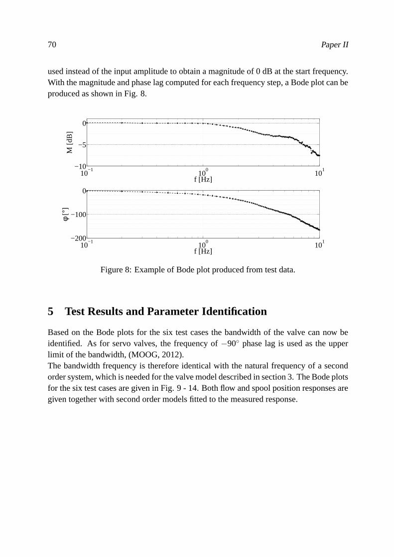
70 Paper II
used instead of the input amplitude to obtain a magnitude of 0dB at the start frequency.With the magnitude and phase lag computed for each frequencystep, a Bode plot can beproduced as shown in Fig. 8.
10−1
100
101−10
−5
0
f [Hz]
M [d
B]
10−1
100
101−200
−100
0
f [Hz]
φ [°
]
Figure 8: Example of Bode plot produced from test data.
5 Test Results and Parameter Identification
Based on the Bode plots for the six test cases the bandwidth of the valve can now beidentified. As for servo valves, the frequency of−90◦ phase lag is used as the upperlimit of the bandwidth, (MOOG, 2012).The bandwidth frequency is therefore identical with the natural frequency of a secondorder system, which is needed for the valve model described insection 3. The Bode plotsfor the six test cases are given in Fig. 9 - 14. Both flow and spool position responses aregiven together with second order models fitted to the measuredresponse.

Modeling, Performance Testing and Parameter Identification... 71
10−1
100
101−10
−5
0
f [Hz]
M [d
B]
2nd order modelSpool positionFlow
10−1
100
101−200
−100
0
f [Hz]
φ [°
]
2nd order modelSpool positionFlow
Figure 9: 5 % amplitude @ 50 % negative offset.
10−1
100
101−10
−5
0
f [Hz]
M [d
B]
2nd order modelSpool PositionFlow
10−1
100
101−200
−100
0
f [Hz]
φ [°
]
2nd order modelSpool PositionFlow
Figure 10: 5 % amplitude @ 50 % positive offset.

72 Paper II
10−1
100
101−10
−5
0
f [Hz]
M [d
B]
2nd order modelSpool PositionFlow
10−1
100
101−200
−100
0
f [Hz]
φ [°
]
2nd order modelSpool PositionFlow
Figure 11: 10 % amplitude @ 50 % negative offset.
The spool position response is used to identify the two modelparameters,ωn andζ .Since the natural frequency can be identified directly from the Bode plots, only thedamping ratio needs to be adjusted to match the measured response.As seen from all six Bode plots, the second order model is not anaccurate descriptionof the valve dynamics. The phase lag of the model fits the measured response quite wellup to around−90◦, but the magnitude does not fit very well.While the dynamics of the valves main stage alone may be modeled as a second ordersystem, the pilot stage and the controller obviously also influence the overall dynamicbehavior of the valve. However, since the proposed valve modelis not intended for de-tailed analysis of the valve itself, but for simulation of hydraulic-mechanical systems,the second order model will, for many applications, be sufficient to capture the valve’sinfluence on the overall system dynamics.The bandwidths and model parameters identified from the testsare listed in Table 2.
For practical reasons the valve has only been tested up to 5 Hz inthe two cases of25 % amplitude, see Fig. 13 - 14. In these two cases the bandwidth cannot be directlyidentified and the data in the last two rows of Table 2 thereforerepresent the best fit ofthe second order model.Considering the remaining data, a reasonable estimate of the bandwidth is 5 Hz, corre-sponding to roughlyωn = 30 rad/s as the natural frequency of the second order modelwith a damping ratio ofζ = 0.8.
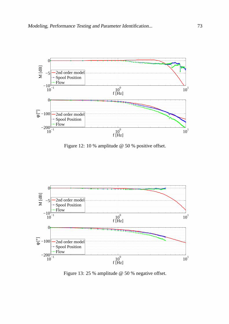
Modeling, Performance Testing and Parameter Identification... 73
10−1
100
101−10
−5
0
f [Hz]
M [d
B]
2nd order modelSpool PositionFlow
10−1
100
101−200
−100
0
f [Hz]
φ [°
]
2nd order modelSpool PositionFlow
Figure 12: 10 % amplitude @ 50 % positive offset.
10−1
100
101−10
−5
0
f [Hz]
M [d
B]
2nd order modelSpool PositionFlow
10−1
100
101−200
−100
0
f [Hz]
φ [°
]
2nd order modelSpool PositionFlow
Figure 13: 25 % amplitude @ 50 % negative offset.

74 Paper II
10−1
100
101−10
−5
0
f [Hz]
M [d
B]
2nd order modelSpool PositionFlow
10−1
100
101−200
−100
0
f [Hz]
φ [°
]
2nd order modelSpool PositionFlow
Figure 14: 25 % amplitude @ 50 % positive offset.
Table 2: Identified bandwidths and models parameters.
Offset[%] Amplitude[%] fBW [Hz] ωn [rad/s] ζ− 50 5 4.5 28.3 0.7+ 50 5 5 31.4 0.6− 50 10 5.5 34.6 0.9+ 50 10 5.2 32.7 0.6− 50 25 7 44 0.9+ 50 25 7 44 0.9
6 Conclusions
In this paper, an approach for dynamic performance testing of pressure compensatedproportional directional control valves (PCPDCVs) has been presented along with iden-tification of parameters for a proposed model of the considered type of valve.In the model, the dynamics of the valves is represented by a second order system andtherefore only requires two parameters. This limits the level of model complexity whilestill capturing the overall dynamic system behavior for simulation of hydraulic-mechanicalsystems.For detailed component analysis, e.g., for design of valves, a second order model is notan adequate representation of the valve dynamics. For that amore detailed model isrequired.As a case study a Sauer-Danfoss PVG32 has been considered. With the presented test

Modeling, Performance Testing and Parameter Identification... 75
approach, the bandwidth has been determined to 5 Hz, corresponding to a natural fre-quency ofωn = 30 rad/s and a damping ratio ofζ = 0.8.
Acknowledgements
The work presented in this paper is funded by the Norwegian Ministry of Education andResearch and Aker Solutions.The authors would like to thank Aker Solutions and Sauer-Danfoss for sponsoring com-ponents used for the experimental work.
Nomenclature
ure f Spool postion reference (control signal) -uspool Spool postion (normalized) -uedge Opening, P-B, A-T, P-A, or B-T edge -uC Opening, compensator -OLedge Overlap, P-B or P-A edge -ULedge Underlap, A-T or B-T edge -Qedge Flow, P-B, A-T, P-A, or B-T edge [m3/s]QC Flow, compensator [m3/s]Cedge Flow coefficient, P-B, A-T, P-A, or B-T edge [m3/s·Pa0.5]Cedge Flow coefficient, compensator [m3/s·Pa0.5]Cd Discharge coeffiecient -Aedge Cross sectional area, fully opened edge [m2]∆pedge Pressure drop, P-B, A-T, P-A, or B-T edge [Pa]pA Pressure, A-port [Pa]pB Pressure, B-port [Pa]pLS Load sensing pressure [Pa]pC Compensated pressure [Pa]p0 Pre-compression, compensator spring [Pa]pS Supply pressure [Pa]KC Stiffness, compensator spring [Pa/−]VC Volume [m3]ρ Density, hydraulic fluid [kg/m3]β Stiffness (bulk modulus), hydraulic fluid [Pa]yA Approximated output [%]OA Approximated offset [%]

76 Paper II
AA Approximated output amplitude [%]A0 Low-frequency output amplitude [%]φA Approximated phase lag [◦]t Time vector [s]M Magnitude [dB]f Test frequency [Hz]fBW Bandwidth frequency [Hz]ωn Natural frequency [rad/s]ζ Damping ratio -
References
Borghi, M., Milani, M., and Paoluzzi, R. (2005). Influence ofnotch shape and numberof notches on the metering characteristics of hydraulic valves. International Journalof Fluid Power, 6(4):5–18.
Gordic, D., Barbic, M., and Jovicic, N. (2004). Modelling of spool position feedbackservovalves.International Journal of Fluid Power, 5(1):37–50.
Institution, B. S. (2009). Bs iso 10770-1:2009. hydraulic fluid power - electrically mod-ulated hydraulic control valves. part 1: Test methods for four port directional flowcontrol valves. Technical report, British Standards Institution.
Käppi, T. and Ellman, A. (1999). Modelling and simulation of proportional mobilevalves. InProceedings of the 4th JHPS International Symposium on Fluid Power,pages 531–536. Tokyo, Japan.
Käppi, T. and Ellman, A. (2000). Analytical methods for definingpressure compensatordynamics.Fluid Power Systems and Technology, 7:121–125.
Liu, X., Huang, Q., Dacheng, C., Han, J., and Lin, X. (2009). Analysis ofperfor-mance effect factors of three-stage electro-hydraulic servo valve. Journal of Com-puter, 4(12):1216–1222.
MOOG (2012). Electrohydraulic valves... a technical look. Technical report, Moog Inc.http://www.moog.com/literature/ICD/Valves-Introduction.pdf.
Opdenbosch, P., Sadegh, N., Book, W., Murray, T., and Yang, R. (2009). Modelling anelectro-hydraulic poppet valve.International Journal of Fluid Power, 10(1):7–15.
Sauer-Danfoss (2013). Pvg proportional valves. http://www.sauer-danfoss.com/Products/PVGProportionalValves/index.htm.

Modeling, Performance Testing and Parameter Identification... 77
Zhang, R., Alleyne, A. G., and Prasetiawan, E. A. (2002). Performance limitations of aclass of two-stage electro-hydraulic flow valves.International Journal of Fluid Power,3(1):47–53.

78 Paper II

Paper IIIModel Based Design Optimization of
Operational Reliability in
Offshore Boom Cranes
Morten Kollerup Bak and Michael Rygaard Hansen
79

80 Paper III
This paper has been published as:
M. K. Bak and M. R. Hansen, “Model Based Design Optimization of Operational Relia-bility in Offshore Boom Cranes”,International Journal of Fluid Power. Vol. 14 (2013),No. 3, pp. 53-65.

Model Based Design Optimization... 81
Model Based Design Optimization of Operational Reliability
in Offshore Boom Cranes
Morten Kollerup Bak and Michael Rygaard HansenDepartment of Engineering Sciences
Faculty of Engineering and Science, University of AgderJon Lilletunsvei 9, 4879 Grimstad, Norway
Abstract — This paper presents a model based approach for design of reliable electro-hydraulic motion control systems for offshore material handling cranes. The approachtargets the system engineer and is based on steady-state computations, dynamic timedomain simulation and numerical optimization.In general, the modeling takes into account the limited access to component data nor-mally encountered by engineers working with system design. Asystem model is pre-sented which includes the most important characteristics ofboth mechanical system andhydraulic components such as the directional control valveand the counterbalance valve.The model is used to optimize the performance of an initial design by minimizing oscil-lations, maximizing the load range and maintaining operational reliability.
Keywords — System modeling, system design, counterbalance valve, directional controlvalve.

82 Paper III
1 Introduction
Despite the fact that hydraulics, in general, is considered amature technology, designof hydraulic motion control systems still offers a number ofchallenges for both com-ponent suppliers and manufacturers of hydraulically actuated machines. For the systemdesigner, the main challenge is to meet the functional requirements for the system, aset of design constraints, while satisfying a number of performance criteria such as cost,weight, overall efficiency and response time, which are often conflicting and also subjectto constraints.Design of hydraulic systems has been subjected to extensive research including steady-state based design, (Stecki and Garbacik, 2002), as well as component selection us-ing dynamic simulation and numerical optimization, (Krus etal., 1991), (Hansen andAndersen, 2001), (Andersson, 2001) and (Papadopoulos and Davliakos, 2004). Auto-mated design through so-called expert systems with the ability to handle both conceptualand detailed design have attracted a considerable amount ofinterest from researchers,(da Silva and Back, 2000), (Hughes et al., 2001), (Liermann and Murrenhoff, 2005) and(Schlemmer and Murrenhoff, 2008). The impact outside academia, however, remainslimited. A reason for this may be that design of hydraulic systems is somewhat appli-cation dependent. Design criteria and constraints in combination with design traditionsdiffer from one application area to another, making it difficult to set up and maintaindesign rules for expert systems. Moreover, scepticism and conservatism may contributeto design engineers being reluctant to make use of such systems.Hydraulic systems are therefore still designed manually andin many cases based on ex-isting systems, reducing the design job to a sizing problem where the system architectureis already given. In these cases the design engineer can certainly make benefit from pre-viously mentioned tools such as dynamic simulation and optimization. However, usingthese tools still requires a great level of application specific knowledge.For offshore applications, which are the focus of this paper,reliability and productivityare the most important performance criteria. They are especially important for offshoreapplications because of remote locations and high cost of down time. Therefore priceand efficiency are less important criteria than for other applications like agriculture orconstruction machines.In the offshore industry, the problem of designing reliablesystems is further complicatedby limited opportunities to build prototypes to verify new designs. This only promotesthe need for model based design approaches wherevirtual prototypescan be used toevaluate and optimize a design.In this paper an offshore material handling application is considered which uses a pres-sure compensated directional control valve (DCV) and a counterbalance valve (CBV) -classically prone to instability and therefore unreliable. A dynamic model and a typical

Model Based Design Optimization... 83
steady-state sizing procedure are presented as seen from a system designer’s point ofview. Next, an optimization procedure, based on the Complex method, is applied in or-der to investigate two different design concepts; one that represents a traditional way ofchoosing design parameters for the considered system and one that represents a new andreliable way of handling the problem of using a pressure compensated DCV togetherwith a CBV. The two methods are compared and their limitationsare discussed.
2 Considered System
The considered system is part of a smaller crane used for material handling on an off-shore drilling rig. It is put forward as a representative problem within offshore cranedesign where the mechanical system and operating cycles are determined a priori.The mechanical system is a crane boom actuated by a hydrauliccylinder, configured asshown in Fig. 1.
4m
1.1
3m
A
B
C
0.5m
1.75m
0.25m
Figure 1: Mechanical system.
The total mass of the boom and the load attached to it is 5000 kgwith COG located at adistance of 4 m from the pivoting point of the boom.The cylinder is controlled with an electro-hydraulically actuated DCV with integratedload sensing (LS) circuit and pressure compensator which maintains an approximatelyconstant pressure drop ofpcomp− pLS= 7·105 Pa across the metering edge of the DCV,see Fig. 2. This makes the controlled flow independent of the load pressure and propor-tional to the position of the DCV main spool.An externally vented (drained) CBV is used to control the piston pressure,p2, duringload lowering, i.e., when the cylinder is exposed to negative loads. The system is sup-plied by a hydraulic power unit (HPU) with constant supply pressure, pS= 210·105 Pa,and return pressure,pR = 0.The control system consists of a feedforward controller (FFC) which is a scaling of thevelocity reference, vref, and a feedback controller (FBC),which is a PI controller thatregulates the actuator position,s, according to the position reference,sre f .

84 Paper III
pS
pR
pcomp pLS
p1
p2
p3
FBC
FFC
sref
vref
F
s
v
Figure 2: Electro-hydraulic motion control system.
This type of electro-hydraulic motion control system is widely used for offshore mate-rial handling equipment where closed loop control of the individual actuators is used toachieve control of a manipulator end point and where several machines are supplied bya common HPU with a ring line system connected to the individualmachines.Design of such a system is an iterative process involving design of both the mechanicalsystem and the motion control system. In practice, detaileddesign of both systems iscarried out separately with constraints imposed by a conceptual design. The conceptualdesign is then revisited if it later proves to be unsuitable.As an example placement and size of the cylinder may be determined during the concep-tual design phase. To ensure the lifting capacity, the required cylinder piston diametercan be obtained by:
Dp ≥√
4π· Fmax
ηhmc· (p2− p3 ·φ)(1)
The forceFmax includes the steady-state load force and, for offshore equipment, a certaincontribution from environmental loads, e.g., wind and waves.The return pressure,p3, can often be neglected or alternatively set to, e.g., 5...10·105 Pato account for the pressure drop through the return path. Theinlet pressure,p2, is typi-cally set to 20...30·105 Pa below the supply pressure, e.g., 180·105 Pa if the supply is210·105 Pa. The hydro-mechanical efficiency,ηhmc, depends on the cylinder design andtype of sealings. In practice it is typically set to 0.9 for the considered type of cylinder,(Rasmussen et al., 1996).Simultaneously, the minimum required rod diameter must be determined in order toavoid buckling of the cylinder. A simple and common approach isto use the rod diam-eter as an effective diameter throughout the length of the whole cylinder and apply the

Model Based Design Optimization... 85
formula forEuler bucklingof an ideal column:
Dr ≥4
√64· fs · (l2 ·F)max
π3 ·E (2)
Since the load on the cylinder varies with the position of the piston the maximum prod-uct of the squared cylinder length,l , and the force,F , is used and an appropriate safetyfactor, fs, is introduced.The system may have several operating cycles which need to be considered when de-signing it. For a crane with coordinated control of multiple actuators, inverse kinematicsmay be applied to obtain the operating cycles for the individual actuators. However,independent operating cycles are usually defined for each actuator and used as designreferences. The most common is to use a trapezoidal velocityprofile to determine themaximum velocity:
vmax=∆s
∆t − tramp(3)
Cylinders are usually required to use the full stroke,h, i.e.,∆s= h. ∆t is the time of theoperating cycle, i.e., time for lifting or lowering, andtramp is the ramping time.Parameters for the cylinder and the operating cycle, for which the motion control systemis to be designed, are given in Table 1.
Table 1: Parameters for cylinder and operating cycle.
Cylinder
Fmax= 195 N ηhmc= 0.9 fs = 4lmin = 1.536 m h= 1 m E = 2.1 ·109 PaDp = 0.125 m Dp = 0.08 m φ = 0.59
Operating cycle
∆t = 10 s tramp= 1.5 s vmax = 0.118m/s
3 System Modeling
In model based design the actual modeling is closely linked to the design objectives. Themain challenge is to minimize the complexity of the system model without ignoring orunderestimating important physical phenomena. For systems manufacturers this chal-lenge involves setting up suitable models of a number of sub-supplier components forwhich the required data may be difficult to acquire or not available. For the considered

86 Paper III
system this includes, among other parameters, the bandwidthof the DCV, steady-statecharacteristics of the CBV and cylinder friction.The model of the hydraulic-mechanical system is developed with MapleSimTM and con-sists of both predefined library components and custom made components developed viaMapleTM. This combination facilitates both efficient model development and modelingat a detail level that is not supported by library components.The design analysis and optimization (section 5) is carriedout with MATLAB R© andSimulinkR©. For this purpose an S-function (compiled C-code) is generated from theMapleSimTM model and used to carry out simulations in SimulinkR©.The advantage of this use of the two software packages is the speed and efficiency withwhich models can be developed in MapleSimTM combined with fast simulation of theS-function in SimulinkR© and predefined functions in MATLABR© for post processingand design optimization.
3.1 Mechanical System
The mechanical system is modelled as a three-dimensional multi-body system with threerigid bodies; boom, cylinder barrel and cylinder piston.The hinges in points A, B and C (see Fig. 1) are modelled as a revolute joint, a sphericaljoint and a universal joint, respectively. The translational degree of freedom (DOF)between the cylinder barrel and piston is modelled as a prismatic joint. This gives asystem with a single DOF which is actuated by the hydraulic cylinder. Fig. 3 shows thechosen model structure as it appears in MapleSimTM.
A
spherical joint
B
universal joint
C
prismatic joint
interface to hydraulic model
boom
cylinder piston
revolute joint
cylinder barrel
Figure 3: Structure of mechanical model.
The flexibility of the boom may have some influence on the system dynamics but is notincluded here.
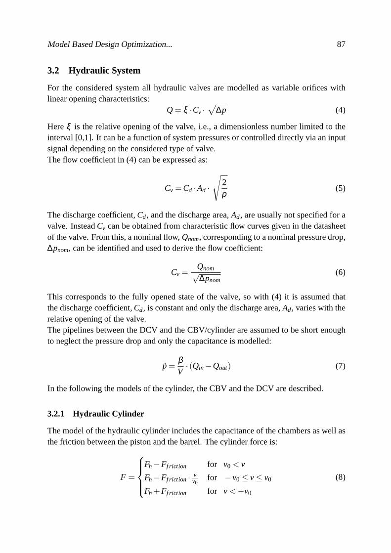
Model Based Design Optimization... 87
3.2 Hydraulic System
For the considered system all hydraulic valves are modelledas variable orifices withlinear opening characteristics:
Q= ξ ·Cv ·√
∆p (4)
Hereξ is the relative opening of the valve, i.e., a dimensionless number limited to theinterval [0,1]. It can be a function of system pressures or controlled directly via an inputsignal depending on the considered type of valve.The flow coefficient in (4) can be expressed as:
Cv =Cd ·Ad ·√
2ρ
(5)
The discharge coefficient,Cd, and the discharge area,Ad, are usually not specified for avalve. InsteadCv can be obtained from characteristic flow curves given in the datasheetof the valve. From this, a nominal flow,Qnom, corresponding to a nominal pressure drop,∆pnom, can be identified and used to derive the flow coefficient:
Cv =Qnom√∆pnom
(6)
This corresponds to the fully opened state of the valve, so with (4) it is assumed thatthe discharge coefficient,Cd, is constant and only the discharge area,Ad, varies with therelative opening of the valve.The pipelines between the DCV and the CBV/cylinder are assumed tobe short enoughto neglect the pressure drop and only the capacitance is modelled:
p=βV· (Qin−Qout) (7)
In the following the models of the cylinder, the CBV and the DCV are described.
3.2.1 Hydraulic Cylinder
The model of the hydraulic cylinder includes the capacitanceof the chambers as well asthe friction between the piston and the barrel. The cylinder force is:
F =
Fh−Ff riction for v0 < v
Fh−Ff riction · vv0
for −v0 ≤ v≤ v0
Fh+Ff riction for v<−v0
(8)

88 Paper III
The hydraulic force isFh = p2 ·Ap− p3 ·φ ·Ap. The actual friction in the cylinder is quitecomplex, especially around zero velocity. As described in Ottestad (2012) it consists ofboth static and coulomb friction as well as velocity dependent and pressure dependentfriction, which may be described with a model of five parameters. Even though themodel is not very complex, the number of parameters represents a problem for a systemdesigner because they need to be experimentally determined.Consequently, an even simpler model must be used:
Ff riction = FS+Cp · |Fh| (9)
The first term is the static friction which may be set toFS ≈ Ap · 1 · 105 m2 · Pa. InOttestad et al. (2012) it was experimentally determined toFS= 580 N for a cylinder ofthe same size as the one used here. The second term is the pressure dependent frictionwhich may constitute 2...3 % of the hydraulic force, e.g.,Cp = 0.02. v0 in Eq. (8) is usedto handle the transition around zero velocity in order to avoid computation difficultiesand can be set to a small value of, e.g.,v0 = 0.005 m/s.Even though the friction model described by Eq. (9) is quite simple, it is sufficient forthe considered system because the operating cycle does not contain any position controlaround zero velocity.The pressure gradients in the two chambers are:
p2 =βV1
· (Q1−v·Ap) (10)
p3 =βV2
· (v·φ ·Ap−Q2) (11)
The chamber volumes,V1 andV2, are functions of the piston position,s. Q1 andQ2 arethe flows on the piston-side and the rod-side of the cylinder, respectively.
3.2.2 Counterbalance Valve
The model of the CBV consists of two components; check valve and pilot assisted reliefvalve (the CBV itself), both modelled according to Eq. (4).The relative opening of the check valve is:
ξcv =p1− p2− pcr,cv
ks,cv(12)
The cracking pressure,pcr,cv, of the check valve is usually specified for a CBV and thenormalized spring stiffness can be set to a value of, e.g.,ks,cv = 1 ·105 Pa.
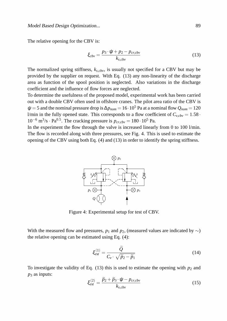
Model Based Design Optimization... 89
The relative opening for the CBV is:
ξcbv=p3 ·ψ + p2− pcr,cbv
ks,cbv(13)
The normalized spring stiffness,ks,cbv, is usually not specified for a CBV but may beprovided by the supplier on request. With Eq. (13) any non-linearity of the dischargearea as function of the spool position is neglected. Also variations in the dischargecoefficient and the influence of flow forces are neglected.To determine the usefulness of the proposed model, experimental work has been carriedout with a double CBV often used in offshore cranes. The pilot area ratio of the CBV isψ = 5 and the nominal pressure drop is∆pnom= 16·105 Pa at a nominal flowQnom= 120l/min in the fully opened state. This corresponds to a flow coefficient of Cv,cbv= 1.58·10−6 m3/s · Pa0.5. The cracking pressure ispcr,cbv= 180·105 Pa.In the experiment the flow through the valve is increased linearly from 0 to 100 l/min.The flow is recorded along with three pressures, see Fig. 4. This is used to estimate theopening of the CBV using both Eq. (4) and (13) in order to identify the spring stiffness.
p3
p2
p1
Q
Figure 4: Experimental setup for test of CBV.
With the measured flow and pressures,p1 andp2, (measured values are indicated by∼)the relative opening can be estimated using Eq. (4):
ξ (1)est =
Q
Cv ·√
p2− p1(14)
To investigate the validity of Eq. (13) this is used to estimate the opening withp2 andp3 as inputs:
ξ (2)est =
p2+ p3 ·ψ − pcr,cbv
ks,cbv(15)

90 Paper III
The spring stiffness is tuned until the best match betweenξ (1)est andξ (2)
est is obtained. Theresult is shown in Fig. 5 together with the input flow. The relative openings are given inpercentage.
0 5 10 15 20 250
20
40
60
80
100
t [s]
Q [
l/min
], ξ
[%]
est
ξest
(1)
ξest
(2)
Figure 5: Estimated and openings and flow and measured flow.
The best match between the two estimated openings is obtainedwith ks,cbv= 295·105
Pa. Also shown in Fig. 5 is the estimated flow obtained by means ofξ (2)est andp1 andp2:
Qest= ξ (2)est ·Cv ·
√p2− p1 (16)
From the correspondence shown in Fig. 5 there seems to be limited influence from flowforces and, although the suggested model is relatively simple, the results show that it isadequate to describe the steady-state characteristics of the considered type of CBV.
3.2.3 Directional Control Valve
The DCV model consists of several smaller models representing the main components ofthe valve; main spool, LS circuit and pressure compensator.The model does not includethe functionality of the electro-hydraulic actuation, butinstead a simplified model of thedynamics between the input signal and the main spool position, represented by a secondorder system:
uspool
ure f=
1s2
ω2v+2 ·ζ · s
ωv+1
(17)
The control signal,ure f , is the sum of the feedforward control signal,uFF , and the feed-back control signal,uFB. The spool position,uspool, is a normalized signal which canvary continuously between -1 and 1, with 0 being the center position of the spool.For servo valves and high-performance proportional valvesthe bandwidth,ωv, can usu-ally be identified from the valves datasheet. For pressure compensated DCVs there isusually no information available about the bandwidth and theonly way to identify it maybe to carry out a frequency response test of the considered valve. An approach for such
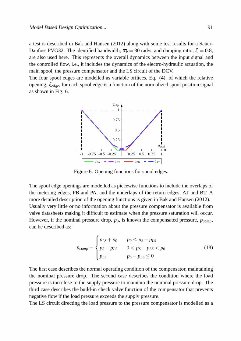
Model Based Design Optimization... 91
a test is described in Bak and Hansen (2012) along with some testresults for a Sauer-Danfoss PVG32. The identified bandwidth,ωv = 30 rad/s, and damping ratio,ζ = 0.8,are also used here. This represents the overall dynamics between the input signal andthe controlled flow, i.e., it includes the dynamics of the electro-hydraulic actuation, themain spool, the pressure compensator and the LS circuit of the DCV.The four spool edges are modelled as variable orifices, Eq. (4), of which the relativeopening,ξedge, for each spool edge is a function of the normalized spool position signalas shown in Fig. 6.
ξedge
0.5 1-0.25-0.5
0.5
ξPB ξATξBTξPA
0.25 0.75
1
0.75
0.25
-1 -0.75
uspool
Figure 6: Opening functions for spool edges.
The spool edge openings are modelled as piecewise functions to include the overlaps ofthe metering edges, PB and PA, and the underlaps of the return edges, AT and BT. Amore detailed description of the opening functions is givenin Bak and Hansen (2012).Usually very little or no information about the pressure compensator is available fromvalve datasheets making it difficult to estimate when the pressure saturation will occur.However, if the nominal pressure drop,p0, is known the compensated pressure,pcomp,can be described as:
pcomp=
pLS+ p0 p0 ≤ pS− pLS
pS− pLS 0< pS− pLS< p0
pLS pS− pLS≤ 0
(18)
The first case describes the normal operating condition of the compensator, maintainingthe nominal pressure drop. The second case describes the condition where the loadpressure is too close to the supply pressure to maintain the nominal pressure drop. Thethird case describes the build-in check valve function of the compensator that preventsnegative flow if the load pressure exceeds the supply pressure.The LS circuit directing the load pressure to the pressure compensator is modelled as a

92 Paper III
piecewise function:
pLS=
p3 uspool< 0
0 uspool= 0
p2 0< uspool
(19)
3.2.4 Model Structure
Fig. 7 shows the model structure of the hydraulic system as it appears in the graphi-cal environment of MapleSimTM. The red lines represent transfer of the two hydraulicpower variables, pressure and flow, between the hydraulic components. The blue linesare signal lines.
hydraulic cylinder
volumevolume
pressure compensator
uref
interface to mechanical model
check valve CBV
LS circuit
PB BT PA AT
p2
p1 p3
pcomp
uspool
pLS
pS
pR
Figure 7: Structure of hydraulic model.
3.3 Control System
In the control system model the velocity reference,vre f , is split into two signals, for lift-ing and lowering, which are scaled by the two feedforward gains, Kv,1 andKv,2 respec-tively, to make up the feedforward controller (FFC). The velocity reference is integratedto obtain the position reference, sref, for the feedback controller (FBC).The structure of the SimulinkR© model, with the control system and the S-function con-taining the hydraulic-mechanical model, is shown in Fig. 8.The input to the hydraulic-mechanical model is the control signal to the DCV, uref inEq. (17). The outputs are the three system pressures,p1, p2 and p3 and the positionof the cylinder piston,s. The latter is used to compute the position error,es = sre f − s,which is the input to the feedback controller (FBC).
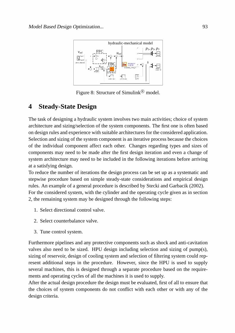
Model Based Design Optimization... 93
vref FFC
srefFBC s
p1, p2, p3
hydraulic-mechanical model
uref
Figure 8: Structure of SimulinkR© model.
4 Steady-State Design
The task of designing a hydraulic system involves two main activities; choice of systemarchitecture and sizing/selection of the system components. The first one is often basedon design rules and experience with suitable architectures for the considered application.Selection and sizing of the system component is an iterativeprocess because the choicesof the individual component affect each other. Changes regarding types and sizes ofcomponents may need to be made after the first design iteration and even a change ofsystem architecture may need to be included in the following iterations before arrivingat a satisfying design.To reduce the number of iterations the design process can be set up as a systematic andstepwise procedure based on simple steady-state considerations and empirical designrules. An example of a general procedure is described by Stecki and Garbacik (2002).For the considered system, with the cylinder and the operating cycle given as in section2, the remaining system may be designed through the followingsteps:
1. Select directional control valve.
2. Select counterbalance valve.
3. Tune control system.
Furthermore pipelines and any protective components such as shock and anti-cavitationvalves also need to be sized. HPU design including selection and sizing of pump(s),sizing of reservoir, design of cooling system and selectionof filtering system could rep-resent additional steps in the procedure. However, since the HPU is used to supplyseveral machines, this is designed through a separate procedure based on the require-ments and operating cycles of all the machines it is used to supply.After the actual design procedure the design must be evaluated, first of all to ensure thatthe choices of system components do not conflict with each other or with any of thedesign criteria.

94 Paper III
4.1 Directional Control Valve
The DCV is selected according to the maximum flow required by theactuator:
Qmax= vmax·Ap (20)
To ensure enough flow for all situations, a valve with a higher capacity may be selected.However this choice is often implicitly made since rated flow ofa valve is a discretedesign variable and the valve with the nearest flow capacity above the required is chosen.For hydraulic systems with closed loop control, an importantproperty of the DCV is thebandwidth. Manufacturers of servo valves usually recommendchoosing a valve with abandwidth,ωv, which is at least three times higher than the natural frequency, ωsys, ofthe system it is used to control, (MOOG, 2012):
ωv ≥ 3 ·ωsys (21)
This applies if the valve should not affect the overall bandwidth of the series connectionof the valve and the hydraulic-mechanical system it is used to control.For many applications such as material handling cranes, it is the opposite, i.e., the band-width of the DCV is lower than the one of the hydraulic-mechanical system. This is alsoreflected by the fact that pressure compensated DCVs have relatively low bandwidths,up to 5 Hz (Bak and Hansen, 2012).Fig. 9 shows the natural frequency of the considered system asfunction of the cylinderpiston position,s, for three different load cases.
0 0.2 0.4 0.6 0.8 10
10
20
30
s [m]
f n [Hz]
100% load50% load25% load
Figure 9: Natural frequency of hydraulic-mechanical system.
Choosing a DCV with a bandwidth of 5 Hz is sufficient for this application as long asthe ramping times for the velocity reference are not too small.

Model Based Design Optimization... 95
4.2 Counterbalance Valve
The size of the CBV is chosen according to the maximum flow required or induced bythe actuator or it may be chosen to match the rated flow of the DCV.In order to avoid unintended opening of the CBV the cracking pressure is typically setto a factor of 1.3 above the maximum load induced pressure, (Sun Hydraulics, 2012):
pcr,cbv≥ 1.3 · pload,max (22)
One of the most critical design variables of a system containing CBVs is the pilot arearatio, ψ, due to its strong influence on the system stability during loadlowering. Itis therefore usually chosen based on experience and may needto be changed once thesystem has been realized and tested.Some basic steady-state considerations for choosingψ may be applied to ensure thatcavitation does not occur on the metering side of the cylinder during load lowering.The cylinder force during negative loads:
F =1
ηhmc· (p2 ·Ap− p3 ·φ ·Ap) (23)
And the opening condition for the CBV:
p2+ψ · p3 = pcr,cbv (24)
Can be combined to express the upper limit ofψ:
ψ ≤pcr,cbv− F ·ηhmc
Ap
p3−φ (25)
p3 is set to the preferred safety margin, e.g., 10...20·105 Pa in order to avoid cavitation.
4.3 Control System
The feedback controller gains cannot be determined based onsteady-state considerationsand therefore have to be tuned after the system has been realized. The feedforward gains,on the other hand, can be estimated when using a pressure compensated DCV.For a DCV with a symmetrical and linear flow characteristic (neglecting the deadband

96 Paper III
of the valve) the cylinder velocity is:
v≈ ure f ·Qmax
AQ(26)
AQ =
{Ap 0≤ ure f
φ ·Ap ure f < 0(27)
In Eq. (26)Qmax is the maximum flow of the valve. With a velocity reference thefeedforward control signal can be computed:
uFF = vre f ·Kv (28)
Combining Eq. (26) and (eq28pap3) yields the feedforward gain:
Kv =AQ
Qmax(29)
4.4 System Characteristics
Employing the sizing procedure described through Eq. (20) -(29) yields a number ofdesign parameters for the considered system. They are listed in Table 2 together withthe most important model parameters. With the velocity reference specified in section 2,
Table 2: Parameters for hydraulic system.
Directional control valve
ωv = 30 rad/s ζ = 0.8Cv = 2 ·10−6 m3/s · Pa0.5 overlap: 10%p0 = 7 ·105 Pa
Counterbalance valve
ψ = 3 Cv=1.58·10−6 m3/s·Pa0.5
pcr,cbv= 235·105 Pa ks,cbv= 300·105 Papcr,cv = 2 ·105 Pa ks,cv = 1 ·105 Pa
Control system
Kv,1 = 7.4 Kv,2 = 4.3
see Fig. 10, a simulation is carried out to analyze the response of the system.With the feedforward gains given in Table 2 and the feedback controller disabled thepiston position shown in Fig. 11 is obtained.

Model Based Design Optimization... 97
0 5 10 15 20 25
-0.1
-0.05
0
0.05
0.1
0.15
t [s]
v [m
/s]
Figure 10: Velocity reference,vre f .
0 5 10 15 20 250
0.2
0.4
0.6
0.8
1
t [s]
s [m
]
sref
s
Figure 11: Position reference,sre f , versus simulated position,s.
The simulated system pressures are shown in Fig. 12.
0 5 10 15 20 25-100
0
100
200
300
400
t [s]
p ⋅
105 [P
a]
p1
p2
p3
Figure 12: Simulated system pressuresp1, p2 andp3.
As seen from both Fig. 11 and 12 the system becomes strongly oscillatory during thelowering sequence and it is not able to follow the prescribed position reference withthe feedforward controller alone. As the last step in a designprocedure the feedbackcontroller can relatively easy be tuned to remove the accumulated position error seen inFig. 11.

98 Paper III
5 Dynamic Considerations
The system response shown in Fig. 11 and 12 illustrates a classical problem with systemsusing a CBV in combination with a pressure compensated DCV. If care is not taken thesystem is likely to become so oscillatory that it is uncontrollable. Furthermore, thenegative values of p3, though they cannot occur in reality, indicate that the oscillationsare violent enough to cause cavitation in rod-side chamber of the cylinder.The system response is directly influenced by the chosen pilot area ratio,ψ, which isusually set high for energy efficiency purposes and only lowered if the system, as in thiscase, becomes strongly oscillatory.From Eq. (25) a pilot area ratio ofψ = 3 is obtained. In Fig. 13 the pressure responsewith ψ = 1 is shown.
0 5 10 15 20 250
50
100
150
200
t [s]
p ⋅
105 [P
a]
p1
p2
p3
Figure 13: Simulated pressures withψ = 1.
Lowering the pilot area ratio clearly reduces the oscillations. However, a significantlevel of oscillation remains and often it is necessary to take extra measures to furtherreduce the oscillations.
5.1 Reliability and Dynamic Performance
Strong oscillations may lead to excessive noise, wear and fatigue, and as shown in Fig.12, loss of functionality. Hence, these oscillations are directly related to the reliabilityof the system.The oscillatory nature of the considered system has been investigated several times(Miyakawa, 1978), (Overdiek, 1981), (Persson et al., 1989),(Handroos et al., 1993),(Chapple and Tilley, 1994), (Ramli et al., 1995), (Zähe, 1995) and (Andersen et al.,2005) and it is well established that it is caused by having twoactive throttling controlvalves in series; the pressure compensator of the DCV and the CBV. The oscillations canbe reduced by lowering the pilot area ratio, bleeding of the CBV’s pilot line or narrowingthe return edge of the DCV. These measures can, however, not remove the oscillatorynature related to the CBV and therefore they do not improve the reliability of the system,

Model Based Design Optimization... 99
they only improve the dynamic performance.Reliability may be divided into several categories, e.g., operational reliability and safetyrelated reliability, and their importance may vary from one application to another. Whileboth types of reliability are important for offshore applications, the first one is the mainconcern here. The operational reliability, i.e., how well and reliable the system can becontrolled, is directly influenced by its oscillatory nature.In order to improve the operational reliability, the concept of two throttling valves in se-ries must be abandoned. This can be done either by removing the pressure compensatoror by removing the CBV. The first measure is normally avoided in offshore applicationsbecause it increases the demands on the feedback controllerand therefore introducesanother loss of operational reliability. The second measure is only partially possiblebecause the CBV has other functionalities than controllingthe load lowering. It can,however, be obtained by forcing the CBV to open completely, asdescribed by Nord-hammer et al. (2012), making it work as a fixed orifice. This will,in turn, require thatthe throttling is handled by the return edge of the DCV.While this eliminates the oscillations caused by the CBV andtherefore improves theoperational reliability, the safety related reliability is likely to be reduced due to an in-creased closing time of the CBV and a possibly increased riskof the CBV getting stuckopen. This is critical in case of hose rupture and therefore the method may need to becombined with safety increasing features or monitoring functions. Further safety assess-ment, however, is not carried out here.Reducing the pilot area ratio of the CBV or transferring the return throttling to the DCVwill reduce the load range that can be handled during lowering.The loss in efficiency,on the other hand, is not a big issue since the considered system is supplied from a ringline with a constant pressure level.Availability becomes an issue if the return throttling is tobe handled by the DCV, sincethis requires a tailor-made main spool whereas a CBV is usually available with severaldifferent pilot area ratios.The oscillatory behavior of the considered system can be investigated by means of sim-ulation. The pilot area ratio and the return edge of the DCV arethe design parametersthat must be chosen with the objective to:
1. Minimize oscillations.
2. Maximize load range.
Simultaneously, it must be chosen if the operational reliability should be increased byforcing the CBV open and if the availability should be reduced by demanding a tailor-made main spool for the DCV.

100 Paper III
5.2 Design Optimization
The most effective way to handle this is by means of numericaloptimization using asuitable algorithm based on minimization techniques. In the following, two differentdesign concepts are subjected to optimization and comparedwith the classical conceptof only lowering the pilot area ratio andthrottling with the CBV. One of them representsa semi-classical concept;throttling with the CBV and the DCV. The other represents anew concept; forcing the CBV to open completely andthrottling with the DCV. Bothdesigns, though, represent less available concepts since they require tailor-made DCVmain spools. For both concepts the design variables are the pilot area ratio of the CBVand the size of the return edge of the DCV. The available range of pilot area ratios isψ = [1,1.5,2,2.5,3,4,5] and it is assumed that the return edge of the DCV main spoolcan be machined within the intervalCv,BT = [0.5 ·10−6,2 ·10−6] m3/s · Pa0.5.
5.2.1 Design Objectives
The first objective is to minimize the oscillations of the load controlling pressure,p2,during the lowering sequence. To determine the oscillationslevel, p2 is first low-passfiltered to determine the steady-state pressure,p(ss)
2 , around which it oscillates. Theoscillations ofp2 can then be found:
p(osc)2 = p2− p(ss)
2 (30)
To obtain a single quantity representing the oscillation level, p(osc)2 is squared and inte-
grated over the time of the lowering sequence:
O=∫ t2
t1
(p(osc)
2
)2dt (31)
Before starting the optimization procedure a nominal oscillation level,Onom, of the initialdesign is found. This is used to obtain a normalized oscillation level (an error) duringthe optimization:
e(1)i =Oi
Onom(32)
Here Oi is the oscillation level of the i’th design suggested bythe optimization routine.For the concept ofthrottling with the CBV and DCV, Eq. (32) is used for the objectivefunction. For the concept ofthrottling with the DCV, an additional objective is used to

Model Based Design Optimization... 101
penalize the design if the CBV is not fully open:
e(2)i = 0.5 · Oi
Onom+0.5 · (1−ξ cbvi) (33)
Hereξ cbvi is the mean value of the CBV opening during the lowering sequence.In both cases two additional objectives must be met; the steady-state level ofp3 cannotexceed 180·105 Pa (to ensure the functionality of the DCV) and the steady-state level ofp2 cannot exceed 250·105 Pa (rated pressure of cylinder). If any of these two implicitconstraints are violated, Eq. (32) and (33) are overruled and the error is set toei = 1.Similarly, violation of explicit constraints (limits of design variables) is penalized bysetting the errorei = 1.The second objective of maximizing the load range is handledby evaluating Eq. (32) or(33) for two load cases; one with a load of 5000 kg (maximum load) and one with a lowerload which is the minimum load the considered design can handle without violating anyof the implicit constraints. The objective function used bythe optimization algorithmcan then be described as:
ei = 0.5 ·e(maxload)i +0.5 ·e(minload)
i (34)
Here, bothe(maxload)i ande(minload)
i are represented by either Eq. (32) and (33) dependingon the considered design concept.
5.2.2 Optimization Procedure
The optimization problem, to minimize ei, is solved with the Complex method (Box,1965) with the modification that violation of both implicit and explicit constraints ishandled by penalization, i.e, settingei = 1 as earlier described.The method is often used for optimization of hydraulic systems and has the advantage ofbeing fast and easy to implement (Andersson, 2001). The structure of the optimizationprocedure is shown in Fig. 14.The initial design,xini = [ψ,Cv,BT] according to Table 2, is evaluated by running a sim-ulation to determine the system pressures, i.e., the response shown in Fig. 12. In thesimulation the feedback controller is disabled and only thefeedforward signal is used tocontrol the system.The nominal oscillation level, Onom, is determined by means of Eq. (30) and (31) andpassed on for evaluation of new designs. Next, a random designpopulation is generatedwithin the limits of the design variables,X lim. The size of the population is twice thenumber of design variables, i.e.,Xpop contains four designs.
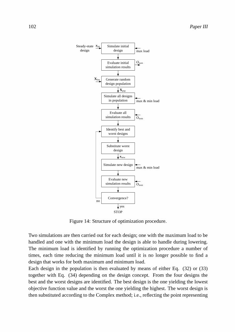
102 Paper III
Simulate initial design
Evaluate initial simulation results
Generate random design population
Simulate all designs in population
Evaluate all simulation results
Identify best and worst designs
Substitute worst design
Simulate new design
Evaluate new simulation results
Steady-state design
xini
X lim
Onom
Xpop
Onom
Convergence?
xnew
Onom
STOP
yes
no
max load
max & min load
max & min load
Figure 14: Structure of optimization procedure.
Two simulations are then carried out for each design; one withthe maximum load to behandled and one with the minimum load the design is able to handle during lowering.The minimum load is identified by running the optimization procedure a number oftimes, each time reducing the minimum load until it is no longer possible to find adesign that works for both maximum and minimum load.Each design in the population is then evaluated by means of either Eq. (32) or (33)together with Eq. (34) depending on the design concept. From the four designs thebest and the worst designs are identified. The best design is the one yielding the lowestobjective function value and the worst the one yielding the highest. The worst design isthen substituted according to the Complex method; i.e., reflecting the point representing

Model Based Design Optimization... 103
the worst design through the centroid of the remaining points in the design space in orderto obtain a new design.A simulation of the new design,xnew, is carried out and the design is evaluated. Theprocedure of substituting the worst design continues untilthe convergence criterion ismet; i.e., the objective function values of the best and the worst design are equal withsome tolerance.
5.2.3 Results
First, the concept of forcing the CBV to open completely andthrottling with the DCVisinvestigated. This is functional in the load range 3000 - 5000 kg (60 - 100 % load) withψ = 5 andCv,BT = 0.7·10−6 m3/s · Pa0.5 as the optimal design values. The pressures forthe maximum and minimum loads are shown in Fig. 15 and 16.
0 5 10 15 20 250
50
100
150
200
t [s]
p ⋅
105 [
Pa]
p1
p2
p3
Figure 15: 100% load,ψ = 5,Cv,BT = 0.7 ·10−6 m3/s · Pa0.5.
0 5 10 15 20 250
50
100
150
200
t [s]
p ⋅
105 [P
a]
p1
p2
p3
Figure 16: 60% load,ψ = 5,Cv,BT = 0.7 ·10−6 m3/s · Pa0.5.
While the oscillations are nearly removed at 60 % load, some oscillations remain at100 % load. This is partly due to the limitp(ss)
3 < 180·105 Pa which prevents furthernarrowing of the return edge. Also, the nature of the system together with the chosenramping time will cause some oscillations as also seen from the lifting sequence.Secondly, the concept ofthrottling with the CBV and the DCVis investigated. This

104 Paper III
is functional in the load range 1500 - 5000 kg (30 - 100 % load) withψ = 1.5 andCv,BT = 0.85·10−6 m3/s · Pa0.5 as the optimal design values. The system pressures forthe two load cases are shown in Fig. 17 and 18.
0 5 10 15 20 250
50
100
150
200
t [s]
p ⋅
105 [P
a]
p1
p2
p3
Figure 17: 100% load,ψ = 1.5,Cv,BT = 0.85·10−6 m3/s · Pa0.5.
0 5 10 15 20 250
50
100
150
200
t [s]
p ⋅
105 [P
a]
p1
p2
p3
Figure 18: 30% load,ψ = 1.5,Cv,BT = 0.85·10−6 m3/s · Pa0.5.
In terms of dynamic performance, i.e., oscillation level, the concept ofthrottling with theCBV and the DCVgenerally yields slightly better results than the concept of throttlingwith the DCV. Both concepts are better than the classical concept ofthrottling with theCBV, in terms of dynamic performance.When considering the operational reliability, however, theconcept ofthrottling withthe DCV is the only fully reliable design because the CBV is active in theother twoconcepts and, inherently, contribute to less predictable system behavior. The evaluationof the different concepts can be summarized as in Table 3.
If only small load variations are to be handled, the concept of forcing the CBV toopen completely andthrottling with the DCVrepresents the best design. For larger loadranges, this may not be a functional design, butthrottling with the CBV and DCVis abetter solution than only throttling with the CBV.Requiring a tailor-made main spool for the DCV represents an additional cost of thesystem. For offshore applications operational reliability is the important performance

Model Based Design Optimization... 105
Table 3: Evaluation of return throttling concepts.
Throttling concept Dynamic perfor-mance
Operational reliabil-ity
DCV + +CBV + DCV + ÷CBV ÷ ÷
criterion and it is therefore often accepted to acquire components with some degree ofcustomization.
6 Conclusions
In this paper, an approach for model based design of electro-hydraulic motion controlsystems for offshore material handling cranes is put forward. The design procedure tar-gets the system engineer and therefore one of the main challenges is to establish reliablesystem models with a suitable level of complexity. Models of the main components ofthe hydraulic system, which include key parameters such as bandwidth of the directionalcontrol valve (DCV) and steady-state characteristics of the counterbalance valve (CBV)is presented.A typical steady-state design procedure is presented and used to determine the parame-ters of the main components of the motion control system. Thepresented system modelis then used to demonstrate the problem of the inherently oscillatory behavior that char-acterizes the considered system.In order to improve the dynamic performance and the operational reliability of the sys-tem, an optimization procedure, based on the Complex method, is applied to the simu-lation model in order to optimize design parameters for the DCV and the CBV.With the objective to reduce the oscillation level during operation of the system, threedifferent design concepts have been investigated:
1. The classical concept,throttling with the CBV, where the pilot area ratio of theCBV is lowered.
2. A semi-classical concept,throttling with the CBV and the DCV, where the pilotarea ratio of the CBV is lowered and the return edge of the DCV is narrowed.
3. A new concept,throttling with the DCV, where the CBV is forced to open com-pletely by increasing the pilot area ratio and narrowing the return edge of the DCV.
The main advantage of the classical concept is availabilityand load range. The mainadvantage of the new concept is operational reliability. The semi-classical concept and

106 Paper III
the new concept both have an advantage in terms of dynamic performance.In an offshore context where operational reliability is the most important criterion, thenew concept is ideal as long as its poor load range capabilityis acceptable, i.e., forapplications with small load variations.
Acknowledgements
The work presented in this paper is funded by the Norwegian Ministry of Education andResearch and Aker Solutions.
Nomenclature
Ad Discharge area [m2]Ap Piston area [m2]AQ Controlled cylinder area [m2]Cd Discharge coefficient -Cv Flow coefficient [m3/s·Pa0.5]Cp Pressure friction coefficient -Dp Piston diameter [m]Dr Rod Diameter [m]e Error/ovjective function value -es Position error [m]E Young’s modulus [Pa]fs Safety factor -F Load force/cylinder force [N]Ff riction Friction force [N]Fh Hydraulic force [N]FS Static friction force [N]h Cylinder stroke [m]ks Normalized spring stiffness [Pa]Kv Velocity feedforward gain -l Cylinder length [m]O Oscillation level -p System pressure [Pa]p0 Nominal pressure drop [Pa]pcomp Compensated pressure [Pa]pcr Cracking pressure [Pa]

Model Based Design Optimization... 107
pload Load induced pressure [Pa]pLS Load sensing pressure [Pa]Q Flow [m3/s]s Piston position [m]t Cycle time [s]tramp Ramping time [s]uFB Feedback control signal -uFF Feedforward control signal -uspool Normalized spool position -ure f Control signal -v Piston velocity [m/s]v0 Transition velocity [m/s]V Volume [m3]β Bulk modulus Paζ Damping ratio -ηhmc Hydro-mechanical efficiency -ξ Relative valve opening -ρ Fluid density [kg/m3]φ Cylinder area ratio -ψ Pilot area ratio -ωsys System natural frequency [rad/s]ωv Valve bandwidth [rad/s]
References
Andersen, T. O., Hansen, M. R., Pedersen, P., and Conrad, F. (2005). The influence offlow forces on the performance of over center valve systems. In Proceedings of theNinth Scandinavian International Conference on Fluid Power. Linköping, Sweden.
Andersson, J. (2001).Multiobjective optimization in engineering design. Applicationsto fluid power systems. PhD thesis, Linköping University, Linköping, Sweden.
Bak, M. K. and Hansen, M. R. (2012). Modeling, performance testingand parameteridentification of pressure compensated proportional directional control valves. InPro-ceedings of the 7th FPNI PhD Symposium on Fluid Power, pages 889–908. ReggioEmilia, Italy.
Box, M. J. (1965). A new method for constrained optimizationand a comparison withother methods.The Computer Journal, 8(1):42–52.
108 Paper III
Chapple, P. J. and Tilley, D. G. (1994). Evaluation techniquesfor the selection of coun-terbalance valves. InProceedings of the Expo and Technical Conference for Electrohy-draulic and Electropneumatic Motion Control Technology, pages 351–359. Anaheim,USA.
da Silva, J. C. and Back, N. (2000). Shaping the process of fluidpower system designapplying an expert system.Research in Enginnering Design, 12(21):8–17.
Handroos, H., Halme, J., and Vilenius, M. (1993). Steady-stateand dynamic proper-ties of counter balance valves. InProceedings of the 3rd Scandinavian InternationalConference on Fluid Power, pages 215–235. Linköping, Sweden.
Hansen, M. R. and Andersen, T. O. (2001). A design procedure for actuator control sys-tem using design optimization. InProceedings of the 7th Scandinavian InternationalConference on Fluid Power. Linköping, Sweden.
Hughes, E. J., Richards, T. G., and Tilley, D. G. (2001). Development of a design supporttool for fluid power system design.Journal of Engineering Design, 12(2):75–92.
Krus, P., Jansson, A., and Palmberg, J.-O. (1991). Optimizationfor component selec-tion in hydraulic systems. InProceedings of the 4th Bath International Fluid PowerWorkshop, pages 219–231. Bath, UK.
Liermann, M. and Murrenhoff, H. (2005). Knowledge based tools for the design ofservo-hydraulic closed loop control.Power Transmission and Control, pages 17–28.
Miyakawa, S. (1978). Stability of a hydraulic circuit with a counterbalance valve.Bul-letin of the JSME, 21(162):1750–1756.
MOOG (2012). Electrohydraulic valves... a technical look. Technical report, Moog Inc.http://www.moog.com/literature/ICD/Valves-Introduction.pdf.
Nordhammer, P., Bak, M. K., and Hansen, M. R. (2012). A method forreliable motioncontrol of pressure compensated hydraulic actuation with counterbalance valves. InProceedings of the 12th International Conference on Control, Automation and Sys-tems, pages 759–763. Jeju Island, Korea.
Ottestad, M., Nilsen, N., and Hansen, M. R. (2012). Reducing the static friction inhydraulic cylinders by maintaining relative velocity between piston and cylinder. InProceedings of the 12th International Conference on Control, Automation and Sys-tems, pages 764–769. Jeju Island, Korea.

Model Based Design Optimization... 109
Overdiek, G. (1981). Design and characteristics of hydraulic winch controls by coun-terbalance valves. InProceedings of the European Conference on Hydrostatic Trans-mission for Vehicle Applications. Achen, Germany.
Papadopoulos, E. and Davliakos, I. (2004). A systematic methodology for optimalcomponent selection of electrohydralic servosystems.International Journal of FluidPower, 5(3):15–24.
Persson, T., Krus, P., and Palmberg, J.-O. (1989). The dynamicproperties of over-centervalves in mobile systems. InProceedings of the 2nd International Conference onFluid Power Transmission and Control. Hangzhou, China.
Ramli, Y., Chapple, P. J., and Tilley, D. G. (1995). Applicationof computer aideddesign (cad) in hydraulic systems using counterbalance valves. InProceedings of the4th International Conference on Computer-Aided Design and Computer Graphics.Wuhan, China.
Rasmussen, P. W., Iversen, F., Halling, B., Haugaard, J., Hounsgaard, G., Mï¿12lbak,H. G., Kristensen, F. D., Lyngbï¿1
2k, E., Rasmussen, N. B., Jessen, B. B., and Jan-nerup, O. (1996).Hydraulik Stï¿12bi. in danish.
Schlemmer, K. and Murrenhoff, H. (2008). Development of an expert system for electro-hydraulic motion control design. InThe 20th International Conference on Hydraulicsand Pneumatics, pages 259–268. Prague, Czech Republic.
Stecki, J. S. and Garbacik, A. (2002). Fluid Power Net Publications.
Sun Hydraulics (2012). Load control and motion control cartridge valves.counterbalance and pilot-to-open check. Technical report,Sun Hydraulics.http://www.sunhydraulics.com/pdf/TT_US_Ctrbal_POCk.pdf.
Zähe, B. (1995). Stability of load holding circuits with counterbalance valves. InPro-ceedings of the 8th Bath International Fluid Power Workshop, pages 60–75. Bath,UK.

110 Paper III

Paper IVAnalysis of Offshore Knuckle Boom Crane
— Part One:
Modeling and Parameter Identification
Morten Kollerup Bak and Michael Rygaard Hansen
111

112 Paper IV
This paper has been published as:
M. K. Bak and M. R. Hansen, “Analysis of Offshore Knuckle Boom Crane— Part One:Modeling and Parameter Identification”,Modeling, Identification and Control. Vol. 34(2013), No. 4, pp. 157-174.

Analysis of Offshore Knuckle Boom Crane — Part One... 113
Analysis of Offshore Knuckle Boom Crane — Part One:
Modeling and Parameter Identification
Morten Kollerup Bak and Michael Rygaard HansenDepartment of Engineering Sciences
Faculty of Engineering and Science, University of AgderJon Lilletunsvei 9, 4879 Grimstad, Norway
Abstract — This paper presents an extensive model of a knuckle boom crane used forpipe handling on offshore drilling rigs. The mechanical system is modeled as a multi-body system and includes the structural flexibility and damping. The motion controlsystem model includes the main components of the crane’s electro-hydraulic actuationsystem. For this a novel black-box model for counterbalancevalves is presented, whichuses two different pressure ratios to compute the flow through the valve. Experimen-tal data and parameter identification, based on both numerical optimization and manualtuning, are used to verify the crane model.The demonstrated modeling and parameter identification techniques target the systemengineer and takes into account the limited access to component data normally encoun-tered by engineers working with design of hydraulic systems.
Keywords — Hydraulic crane, multi-body system, flexibility, directional control valve,counterbalance valve.

114 Paper IV
1 Introduction
Today’s offshore drilling equipment is characterized by high price, high level of systemcomplexity and low production numbers. For the equipment manufacturers, it requires agreat level of skill and experience to develop the equipment, since there are very limitedpossibilities to build prototypes for testing and verification of new designs. Increasingfocus on production and development costs adds to this challenge. As a consequence,design engineers continuously have to improve their procedures for decision making re-garding choice of principal solutions, components and materials in order to reach thebest possible trade-off between different performance criteria such as reliability, effi-ciency and cost.Computer based time domain simulation and optimization techniques have, by far, proventhemselves as excellent tools for the challenged designer and have over the last coupleof decades increasingly been employed by drilling equipment manufacturers. However,the use of these techniques still offers a number of challenges both in industry as well asacademia.In model based design, simulation models serve as virtual prototypes providing informa-tion, e.g., about a machine’s overall efficiency, stabilityand accuracy, enabling engineersto test, redesign and optimize the design of the machine before it is manufactured. Modelbased design offers the possibility to reduce both development time and costs while alsoproducing more reliable machines.The main challenge in model based design lies within the ability to produce simulationmodels that, with a reasonable precision, are able to mimic the behavior of a real system.This challenge is especially pronounced for hydraulicallyactuated machines, like manyoffshore drilling applications, simply because suppliersof hydraulic component are notused to deliver all the data needed to develop simulation models of their products.An application that represents a typical piece of high-end offshore equipment is theknuckle boom crane. The ability to employ a model based approach for design of suchcranes is highly relevant.Modeling, simulation, design and control of various types of cranes have been subjectedto extensive research. General modeling techniques and different control concepts havebeen presented by Hiller (1996) and Abdel-Rahman et al. (2003)and particularly mo-bile (truck-mounted) cranes have attracted a considerableamount of interest from re-searchers (Ellman et al., 1996), (Mikkola and Handroos, 1996), (Esque et al., 1999),(Hansen et al., 2001), (Nielsen et al., 2003) and (Esque et al.,2003). The dynamics ofthese types of cranes is well documented and modeling techniques have been proventhrough experimental verification.In (Than et al., 2002) and (Bak et al., 2011) offshore boom cranes have been investigated.Models taking the structural flexibility into account have been presented, however, with-

Analysis of Offshore Knuckle Boom Crane — Part One... 115
out any experimental verification.Though mobile cranes are particularly flexible and behave differently than offshorecranes, the same modeling techniques can be used for both types of cranes. Modelingof mechanical systems such as boom mechanisms can be handledwith different genericapproaches. However, the most suitable approach is not alwaysobvious.Modeling approaches for hydraulic components and systems are, in general, also well-established but may cause problems when it comes to model verification. The problem isoften a lack of proper model data and/or that the physics is not fully understood. There-fore, for certain hydraulic components, there may be a need to introduce new modelingapproaches.In this paper an extensive model of an offshore knuckle boom crane is developed witha view to identify a best practice for predicting the behavior of this type of crane. It isdemonstrated how to overcome the modeling challenge by choosing an appropriate levelof modeling detail and by using experimental work together with parameter identifica-tion techniques.A commercially available software package, MapleSimTM, is used to develop a dynamicmodel and MATLABR© is used for steady-state simulations and optimization based pa-rameter identification.
2 Considered System
Knuckle boom cranes are used for a wide range of offshore and marine operations andtherefore exist in different variations. The considered crane is manufactured by AkerSolutions and is used on drilling rigs to move drill pipes between the pipe deck and atransportation system leading to the drill floor of the rig.Prior to commissioning of a crane, it undergoes a test procedure to verify the functional-ity and ensure that the performance corresponds to the criteria given in the design spec-ification. This procedure facilitates an experimental study that can be used to calibrateand verify design models of the crane. In the following a description of the consideredcrane is given along with system variables that have been measured and recorded duringa test procedure. The procedure itself is described in section 5 along with the modelparameter identification.The considered crane may be treated as a large multi-domain system consisting of threeinteracting systems:
1. A mechanical system.
2. An electro-hydraulic actuation system.
3. An electronic control system.

116 Paper IV
The main components of the cranes mechanical system are a rotating part mounted on apedestal, an inner jib, an intermediate jib, an outer jib anda gripping yoke, see Fig. 1.
Inner jib
Intermediate jib
Outer jib
Gripping yoke
Rotating part
Pedestal
Pipe deck
7.2
m
12.1
m
2.3 m
10.4
m
Figure 1: Main components of mechanical system.
The crane is controlled from the operators cabin (not shown) mounted on the rotatingpart, also called the king. A slewing bearing and transmission between the king and thepedestal allows for slewing of the crane. However, this degree offreedom (DOF) andthe details of the slewing transmission are not considered here.The gripping yoke also includes a number of hydraulically actuated DOFs which arenot considered. The actuation system is supplied by a hydraulic power unit (HPU) withconstant supply pressure,pS= 210 bar, and return pressure,pR = 0.The considered part of the actuation system consists of three hydraulic circuits, one foreach crane jib, connected to the supply and return lines of the HPU. The control systemincludes a human-machine interface (HMI) which facilitates the operation of the crane,a number of sensors and instruments used for feedback control and/or monitoring and acontroller where the control logic is defined.When considering the actuation and control systems together, the three circuits of theactuation system can be considered as three sub-systems of the motion control system,including both actuation and control. A simplified schematic of the motion control sub-system for the inner jib is shown in Fig. 2.

Analysis of Offshore Knuckle Boom Crane — Part One... 117
pS
pR
p2
p3
Controller
uJS
uV
lcyl
CBV
I
p1
I
IDCV
Figure 2: Simplified schematic of motion control sub-systemfor inner jib.
The main components of the hydraulic circuit are a cylinder with integrated positionsensor, a servo-type directional control valve (DCV) and an externally vented (drained)counterbalance valve (CBV). The cylinder velocity is controlled via the DCV, whichcontrols the flow into either of the two cylinder chambers. During retraction of thecylinder (load lowering), it is exposed to negative loads (piston velocity and load forcehave the same direction) and therefore the piston pressure,p2, needs to be controlled.This is handled by the CBV, which provides a relief valve functionality on the outlet sideassisted by the pressure,p3, on the inlet side.The DCV is controlled via a joystick (part of the HMI) from which the command signal,uJS, is fed to the controller and used to generate the control signal,uV , to the valve. Thesignal from the position sensor in the hydraulic cylinder isalso fed to the controller,where it can be used for feedback control depending on the selected control mode. Inopen loop control mode joystick commands are passed throughthe controller and feddirectly to the DCV. In closed loop control mode both joystickcommands and cylinderpositions are used for control of the DCV.The motion control sub-systems for the intermediate and outer jibs are identical andcontain the same control system elements as the one for the inner jib. However, as seenfrom Fig. 3, the elements of the actuation systems are different.The DCV is pressure compensated and uses a load sensing (LS) circuit and a pressurereducing valve that maintains a constant pressure drop across metering edge of the mainspool at any time. This makes the controlled flow independentof the load pressure andproportional to the spool position, i.e., the control signal fed to the valve.There are two CBVs since the load force on the cylinder may act ineither direction,depending on the orientation of the crane jibs. The CBVs are non-vented and include two

118 Paper IV
pS
pR
pcomp pLS
p2 p3
p1 p4
Controller
uJS
uV
lcyl
px,1 px,2
CBV1 CBV2II
DCV
Figure 3: Simplified schematic of motion control sub-systemfor intermediate and outerjibs.
series connected orifices to manipulate the pilot pressures, px,1 and px,2. For practicalreasons it is only possible to measurep2 andp3 this circuits.In total seven pressures, three command signals and three position signals are measuredand recorded during the experimental test procedure. Table1 provides an overview ofthe system variables and the ones that are measured for the three considered motioncontrol sub-systems.
Table 1: System variables for considered motion control sub-systems.
✓ = measured Input Output State variables
✗ = not mea-sured
uJS lcyl p1 p2 p3 p4 px,1 px,2
Inner jib ✓ ✓ ✓ ✓ ✓ NA NA NAIntermediate jib ✓ ✓ ✗ ✓ ✓ ✗ ✗ ✗Outer jib ✓ ✓ ✗ ✓ ✓ ✗ ✗ ✗
3 Mechanical System Model
The mechanical system is modeled using the multi-body library in MapleSimTM. Themodel includes the main components shown in Fig. 1 as well as the hydraulic cylindersfor the three crane jibs.

Analysis of Offshore Knuckle Boom Crane — Part One... 119
In terms of kinematic structure, the crane can be treated as alarge mechanism consistingof both rigid and flexible links connected by revolute joints. The structural flexibility ofa crane similar to the one considered here has been studied byHenriksen et al. (2011)and Bak et al. (2011). It was shown that the flexibility of certain structural members canhave a significant influence on the overall dynamic behavior of the crane and thereforemust be accounted for in a dynamic model.Here thefinite segment methodis used to model the flexibility. The main advantageof this method is that it is based on rigid body modeling techniques, making it easy toimplement. The method was originally developed by Huston (1981) and further studiedin Huston (1991), Huston and Wang (1993), Connelly and Huston (1994a) and Connellyand Huston (1994b). Hansen et al. (2001) used the method for modeling of a mobilecrane and achieved encouraging results in terms of conformity between measurementsand simulations.The masses, inertias and geometry of the mechanical components have been extractedfrom CAD models.
3.1 Kinematic Structure
The topology of the crane is globally an open kinematic chain, formed by the crane jibs,with locally closed chains formed by the hydraulic cylinders. With the main componentsand the barrels and pistons of the three hydraulic cylinders, the model includes a total of12 bodies, see Fig. 4.Since the slewing DOF of the crane is not considered, the crane can be modeled as a pla-nar mechanism using revolute and translational joints. However, only spatial multi-bodyelements are available in MapleSimTM, making the selection of kinematic constraintsless straight forward. To identify a suitable kinematic structure the crane is initiallytreated as a rigid body system.The bottom of the pedestal is fixed at the global origin and theking is fixed to the topof the pedestal in point A. Points B, C, D and E represent revolute joints (RJ). The con-nection points of cylinder barrels, points F, H and J, are modeled as spherical joints (SJ)while the connection points for pistons, points G, I and K, are modeled as universal joints(UJ). The translational DOFs between the cylinder barrels and pistons are modeled asprismatic joints (PJ). This leaves four remaining DOFs (Nikravesh, 1988):
nDOF = 6 ·nbodies−6 ·nf ixtures−5 ·nPJ
−5 ·nRJ−4 ·nUJ−3 ·nSJ
= 72−12−15−20−12−9= 4
(1)

120 Paper IV
Y X
Z
A
B
C D
E
F
G
H
IJ
K3
4
5
6
7
8
9
2
10
11
12
1
z 3 x 3
z4
x4
z5
x5
z6
x6
Figure 4: Topology of mechanical system model.
These are the ones of the three crane jib, which are actuated byhydraulic cylinders, andthe rotational DOF of the gripping yoke (point E). The latter isactuated by a hydraulicmotor, which is not considered here. The DOF is included to be ableto orientate and fixthe gripping in the wanted positions.
3.2 Flexibility
When applying the finite segment method to a planar mechanism, the flexible membersare divided into a number of rigid segments which are connected by revolute joints androtational springs (and dampers), see Fig. 5.
kS
21
kS kS kSkC
Figure 5: Concept of the finite segment method.
The left part of the figure illustrates a model of a single segment. The flexibility of thesegment is represented by two rotational springs, both with the stiffnesskS. In the rightpart of the figure two segments are connected. The stiffnesskC of the connection between

Analysis of Offshore Knuckle Boom Crane — Part One... 121
the segments corresponds to a series connection of the springs for the two adjoiningsegments:
kC =1
1kS,1
+ 1kS,2
(2)
kS,1 is the segment stiffness of the segment 1 andkS,2 is the segment stiffness of thesegment 2.For bending the segment stiffness is:
kS=2 ·E · I
L(3)
E is the Young’s modulus,I is the area moment of inertia andL is the length of thesegment.The pedestal, the inner jib and the outer jib are assumed to dominate the overall struc-tural flexibility of the crane since the remaining components are far more compact. Fig.6 shows the segmentation of the three flexible members.
s1(1)
s2(1)
s1(3) s2
(3)
s3(3)
s4(3)
s5(3)
s1(5)
s2(5)
s3(5)
s4(5)
kC(1)
kS,1(1)
kS,2(1)
kS,2(3)
kC,1(3)
kC,2(3)
kS,4(3)
kS,2(5)
kC(5)
kS,3(5)
Figure 6: Segmentation of flexible model.
The pedestal, inner jib and outer jib (body numbers 1, 3 and 5)are divided into two, fiveand four segments, respectively. The number of segments is certainly debatable, but iskept low for computational reasons.

122 Paper IV
As seen from Fig. 6, the inner and outer jibs are beam-like structures with varying crosssections. With the chosen segmentations, the cross sectionareas of the individual seg-ments vary linearly and continuously and therefore averagevalues of the segments areamoments of inertia are used to determine the segment stiffnesses,kS. The area momentsof inertia at the cross sections between the segments are extracted from CAD modelsand used to determine the average area moments of inertia. Henriksen et al. (2011) usedthis approach for a model of a single crane jib and compared both static deflections andnatural frequencies of a finite segment model with results of afinite element analysisand achieved a remarkable conformity even without calibrating the model.The segment and connection stiffnesses, determined using (2) and (3), are given in Table2. The first and last segments of the inner and outer jibs are assumed rigid and thereforethe stiffness,kS, of the neighboring segment is used as the connection stiffness,kC.
Table 2: Segment and connection stiffnesses.
Segment kS [Nm/rad] kC [Nm/rad]
s(1)1 5.75·1092.88·109
s(1)2 5.75·109
s(3)1 rigid1.96·109
s(3)2 1.96·1096.03·108
s(3)3 8.73·1082.77·108
s(3)4 4.05·1084.05·108
s(3)5 rigid
s(5)1 rigid2.08·108
s(5)2 2.08·1088.33·107
s(5)3 1.39·1081.39·108
s(5)4 rigid
The stiffnesses in the appliedlumped parameter modelare indeed uncertain (soft) pa-rameters and (2) and (3) merely represent a means to estimatethose parameters. Asargued by Shabana (1997), they can also be determined by finite element analysis andparameter identification. This is, however, not the scope of this paper and instead thestiffnesses are tuned during the calibration (section 5) ofthe entire crane model.

Analysis of Offshore Knuckle Boom Crane — Part One... 123
3.3 Damping
The dynamic characteristics of the mechanical model dependon the damping appliedto it and therefore the damping must be carefully considered. However, damping pa-rameters are even more uncertain than those related to the flexibility. The only way toproperly determine the damping parameters may be to carry out a thorough experimentalstudy of the considered structure. As in this case, time, resources and practical circum-stances seldom allow for that kind of investigations.Therefore, whether working with design models or models for analysis and with limitedpossibilities for experimental investigations, there is aneed for methods to determinethe damping parameters with a reasonable accuracy. Mostofi (1999) presents a simpleapproach that can be used for lumped parameter modeling techniques such as the finitesegment method. Forstiffness damping(damping elements in parallel with the flexibleelements), the damping of a structural member is:
c= βk ·k (4)
k contains the spring coefficients determined in section 3.2 andβk is a stiffness multiplierdetermined by:
βk =2 ·ζS
ωS(5)
ζS is the damping ratio of the structure andωS is the natural frequency of the structurefor the considered mode of motion. Representative damping ratios for different struc-tures are given in Adams and Askenazi (1999). For metal structures with joints, e.g.,weldings and bolted connections, the damping ratio isζ = 0.03−0.07. Naturally, thisis subject to uncertainty but, nevertheless, better than a simple guess.To determine the damping coefficients for the models of the three flexible members,simulations without damping have been carried out to find the natural frequency of eachmember. In the simulations each member is fixed in one end (cantilevered) and an im-pulse is applied to excite oscillations from which the natural frequency can be observed.The natural frequencies and corresponding range of stiffness multipliers for the threeflexible members are given in Table 3.
Table 3: Natural frequencies and stiffness multipliers.
Member ωS [rad/s] βk [s]
Pedestal (with king) 94 0.0006 - 0.0015Inner jib 60 0.001 - 0.002outer jib 35 0.002 - 0.004

124 Paper IV
The stiffness multipliers are tuned together with spring coefficients during the modelcalibration in section 5.
4 Motion Control System Model
Whereas the model of the mechanical system, in general, is based on physical (white-box) modeling, the motion control system model is mostly based on semi-physical (grey-box) modeling. The main reason for this is that manufacturers of hydraulic componentsdo not provide enough and sufficiently detailed informationto establish physical mod-els. In addition, physical models will quickly become too complex and computationaldemanding for system simulation. Therefore certain model structures have to be as-sumed which allow for simplifications without ignoring or underestimating importantphysical phenomena.The motion control system is modeled using both predefined components from the hy-draulic and the signal block libraries in MapleSimTM and custom made componentsdeveloped via MapleTM. This combination facilitates both efficient model developmentand modeling at a detail level that is not supported by library components.Joystick commands and control signals are represented by normalized signal, which canvary continuously between -1 and 1, and component dynamics ismodeled using transferfunctions.Hydraulic valves are generally modeled as variable orifices with linear opening charac-teristics:
Q= ξ ·CV ·√
∆p (6)
Hereξ is the relative opening of the valve, i.e., a dimensionless number between 0 and1. It can be a function of system pressures or controlled with an input signal dependingon the considered type of valve.Q is the volume flow through the valve and∆p is thepressure drop across it.The flow coefficient in (6) can be expressed as:
CV =Cd ·Ad ·√
2ρoil
(7)
The discharge coefficient,Cd, and the discharge area,Ad, are usually not specified for avalve. InsteadCV can be obtained from characteristic flow curves given in the datasheetof the valve. From this, a nominal flow,Qnom, corresponding to a nominal pressure drop,

Analysis of Offshore Knuckle Boom Crane — Part One... 125
∆pnom, can be identified and used to derive the flow coefficient:
CV =Qnom√∆pnom
(8)
This corresponds to the fully opened state of the valve, so with (6) it is assumed thatthe discharge coefficient,Cd, is constant and only the discharge area,Ad, varies with therelative opening of the valve.This modeling approach works well for DCVs with closed loop spoolposition controlwhere dither is used to eliminate static friction and certaindesign details are used toreduce the disturbances from flow forces.In some cases the approach may also work for pressure controlvalves like CBVs. Mostoften, though, attempting to establish physical or semi-physical models of such valveswill encounter a number of challenges, e.g., related to friction and resulting hysteresis,non-linear discharge area characteristics, varying discharge coefficients and varying flowforces. Therefore, a better way to model those types of valves may be to use a non-physical (black-box) approach as described in section 4.2.The following sub-sections describe models of the DCVs, the CBVsand the hydrauliccylinders.
4.1 Directional Control Valves
The main concern, when modeling a DCV, is the steady-state flow characteristics andthe dynamics (bandwidth) of the valve. For system simulations, the design details ofthe valve are usually not important and therefore servo valves and pressure compen-sated DCVs can often be represented by the same model. Breakingdown the model intoseveral elements offers flexibility and facilitates changes in the model like including orexcluding a pressure compensator. The general DCV model includes a representationof the valve actuation (pilot stage) and four elements for the main spool. For pressurecompensated valves, the model also includes the LS circuit and the pressure compen-sator. The model structure for the pressure compensated DCV is shown in Fig. 7. Theblue lines are signal lines transferring only a single statevariable. The red lines transferthe two hydraulic state variable, pressure and flow, between the hydraulic components.These are custom made components developed in MapleTM.The valve is actuated with the control signaluV , which is passed through a second ordersystem representing the dynamics of the valve:
uspool
uV=
1s2
ω2V+2 ·ζV · s
ωV+1
(9)

126 Paper IV
pcomp
pS pR
pB pA
LS circuit
pLS
uVuspool
pressure compensator
PB BT ATPA
Figure 7: Structure of DCV model.
The output,uspool, is a normalized signal representing the spool position, which can varycontinuously between -1 and 1 with 0 being the center position of the spool. The naturalfrequency,ωV , represents the bandwidth of the valve andζV is the damping ratio.For servo valves the bandwidth can usually be identified from the valves datasheet. Herethe valve dynamics is usually visualized with Bode plots for several input amplitudesshowing that the dynamics is non-linear. For system simulations, though, a linear modellike the second order system will most often be sufficient to capture the dominant dy-namics.For pressure compensated DCVs there is usually no informationavailable about thebandwidth and the only way to identify it may be to carry out a frequency responsetest of the considered valve. An approach for such a test is described in Bak and Hansen(2012) along with some test results for a Danfoss PVG32, which is identical to the DCVsused for the intermediate and outer jibs. The identified bandwidth, ωV = 30 rad/s, anddamping ratio,ζV = 0.8, are therefore also used here. This represents the overall dy-namics between the control signal and the controlled flow, i.e., the dynamics of the pilotstage, the main spool, the LS circuit and the pressure compensator.The four main spool edges are modeled as variable orifices, according to (6), for whichthe relative opening,ξedge, of each spool edge is a function of the normalized spool po-sition signal as shown in Fig. 8.The spool edge openings are piecewise linear functions that include the overlaps of themetering edges, PB and PA, and the underlaps of the return edges, AT and BT. A moredetailed description of the opening functions is given in Bak and Hansen (2012).When modeling pressure compensated DCVs, a problem often encountered is that verylittle or no information about the pressure compensator is available from the valvesdatasheet. This makes it difficult to estimate when the pressure saturation will occurand to establish a model of the compensator. However, if the nominal pressure dropacross the main spool metering edge (setting of compensatorspring),p0, is known the

Analysis of Offshore Knuckle Boom Crane — Part One... 127
ξedge
0.5 1-0.25-0.5
0.5
ξPB ξATξBTξPA
0.25 0.75
1
0.75
0.25
-1 -0.75
uspool
Figure 8: Opening functions for spool edges.
compensated pressure,pcomp, can be described as:
pcomp=
pLS+ p0 for p0 ≤ pS− pLS
pS− pLS for 0< pS− pLS< p0
pLS for pS− pLS≤ 0
(10)
The first case describes the normal operating condition of the compensator, maintain-ing the nominal pressure drop across the main spool meteringedge. The second casedescribes the condition where the load pressure is too close to the supply pressure tomaintain the nominal pressure drop. The third case describes the build-in check valvefunction of the compensator, which prevents negative flow if the load pressure exceedsthe supply pressure.The LS circuit directing the load pressure to the pressure compensator is modeled as apiecewise function:
pLS=
pA for uspool< 0
pB for 0< uspool
0 otherwise
(11)
The model parameters for the servo valve (inner jib) and the pressure compensatedDCVs (intermediate and outer jibs) are given in Table 4.
4.2 Counterbalance Valves
The model of the CBV consists of two components; a check valveand a pilot assistedrelief valve (the actual CBV).

128 Paper IV
Table 4: DCV model parameters.
Inner jib Int. & outer jibs
ωV 250 rad/s (40 Hz) 30 rad/s (5 Hz)ζV 0.8 0.8Overlap 5 % 10 %Underlap 0 5 %CV 111.8 l
min·bar0.537.8 l
min·bar0.5p0 NA 7 bar
The check valve is modeled according to (6) with the relative opening given by:
ξCV =p1− p2− pcr,CV
ks,CV(12)
This is only the basic part of a piecewise function that limitsthe relative opening to theintervalξCV = [0,1]. p1 is the pressure at the port connected to the DCV andp2 is thepressure at the port connected to the cylinder. The crackingpressure,pcr,CV, is usuallyspecified for a CBV and the normalized spring stiffness can beset to a low value of, e.g.,ks,CV = 1 bar.In practice the check valve is either opened or closed. The spring stiffness is only used tohandle the transition between the two states, which otherwise may cause computationaldifficulties.Describing the relative opening by means of a pressure equilibrium like (12) can in somecases also be used for the CBV itself. However, for the previously mentioned reasons, itis often only valid for the condition where the CBV is just about to open (crack). For anexternally vented CBV, like the one in Fig. 2, the cracking condition is described by:
p2+ψ · px = pcr,CBV (13)
Once again,p2 is the pressure at the port connected to the cylinder.px is the pilotpressure andψ is the pilot area ratio.For a non-vented CBV, like the one in Fig. 3 (ignoring the two internal orifices), thecracking condition is:
p2+ψ · px = pcr,CBV+(1+ψ) · p1 (14)
As for the check valve,p1 is the pressure at the port connected to the DCV.Instead of using (6) and a pressure equilibrium to model the CBV it is proposed to use ablack-box approach based on the cracking condition in (13).
Analysis of Offshore Knuckle Boom Crane — Part One... 129
For the black-box model, two new variables are introduced;µx andµL. The first one isthe ratio between the pilot pressure,px, and the load pressure,pL:
µx =px
pL(15)
The second variable is dependent on the type of CBV. For an externally vented CBV, itis the ratio between the load pressure and the cracking pressure:
µL =pL
pcr,CBV(16)
For a non-vented CBV, it is the ratio between the pressure dropacross the valve and thecracking pressure:
µL =∆p
pcr,CBV(17)
By replacingp2 with pL in (13) it can be combined with (15) and (16) to arrive at thefollowing expression:
µL,cr =1
1+ψ ·µx(18)
This expression, just as (13) and (14), describes the cracking condition of the CBVwhere there is still no flow the through the valve. It is illustrated by the solid line in Fig.9, here for a CBV with a pilot area ratio ofψ = 3. The dashed lines above illustrateconditions with different levels of flow through the valve.In the model the actualµx andµL for a given time step is computed by (15) and either(16) or (17) depending on the type of CBV. The distance,s, from the cracking line(randomly shown in Fig. 9) is then computed:
s= µL −µL,cr (19)
If the distance is negative, there is no flow through the valve. Otherwise, the flow iscomputed as:
QCBV = ACBV ·snCBV (20)
HereACBV is given by:ACBV = A0+A1 ·µx (21)
Similarly, nCBV is given by:nCBV = n0+n1 ·µx (22)
The four parameters,A0, A1, n0 andn1 have to be experimentally determined, ideally bya thorough mapping of the flow through the CBV for different pressure combinations at

130 Paper IV
0 0.5 1 1.5 20
0.2
0.4
0.6
0.8
1
1.2
1.4
1.6
1.8
2
µx
µ L
Q = 0Q > 0
s
Figure 9: Example of the relation betweenµL andµx for the CBV model.
the individual ports. Alternatively, as described in section 5.2, they can be determinedwith parameter identification techniques and suitable measurements from the systemwhere the CBV is installed.The remaining (known) model parameters for the CBVs and the check valves for theinner jib and the intermediate and outer jibs are given in Table 5.
Table 5: CBV model parameters.
Inner jib Int. & outer jibs
CV 89.4 lmin·bar0.5
63.2 lmin·bar0.5
pcr,CV 1 bar 1 barks,CV 1 bar 1 barpcr,CBV 250 bar 250 barψ 3 6

Analysis of Offshore Knuckle Boom Crane — Part One... 131
4.3 Hydraulic Cylinders
The model of the hydraulic cylinder includes the capacitanceof the chambers as well asthe friction between the piston and the barrel. The cylinder force is:
Fcyl =
Fp−Ff r for vcyl < v0
Fp−Ff r · vcylv0
for −v0 ≤ vcyl ≤ v0
Fp+Ff r for vcyl <−v0
(23)
The pressure force isFp = p1 ·Ap − p2 · φ ·Ap. HereAp is the piston area andφ =
(D2p −D2
r )/D2p, whereDp is the piston diameter andDr is the rod diameter.p1 and
p2 are the pressures in the corresponding cylinder chambers.vcyl is the cylinder pistonvelocity andv0 is a transition velocity used to handle the change in friction force aroundzero velocity.The capacitance of the two chamber volumes are accounted forby:
p1 =βoil
V1· (Q1−vcyl ·Ap) (24)
p2 =βoil
V2· (vcyl ·Aa−Q2) (25)
βoil is the effective stiffness (bulk modulus) of the hydraulic fluid. Q1 andQ2 are volumeflows in the two cylinder chambers. The chamber volumes,V1 andV2, are functions ofthe cylinder length.The friction in the cylinder is quite complex, especially around zero velocity. As de-scribed in Ottestad et al. (2012) it consists of both static and Coulomb friction as wellas velocity dependent and pressure dependent friction, which may be described with amodel of five parameters. Even though the model is not very complex, the number ofparameters represents a problem because they cannot be determined without an exten-sive experimental study of the considered cylinder.Consequently, an even simpler model must be used and therefore the friction force in(23) consists only of static friction and pressure dependent friction:
Ff r = FS+Cp · |Fp| (26)
The static friction can be set toFS = Ap ·1 ·105 m2·Pa, i.e., a pressure of 1 bar on thepiston-side is required to overcome the static friction. The pressure dependent frictionmay constitute 2...3 % of the hydraulic force, e.g.,Cp = 0.02. The friction parametersare identified in section 5. The remaining (known) parametersfor the cylinders are given

132 Paper IV
in Table 6.
Table 6: Cylinder model parameters.
Inner jib Int. & outer jibs
Dp 0.3 m 0.25 mDr 0.18 m 0.125 ml0 3.145 m 2.315 mstroke 1.755 m 1.33 mmass 1500 kg 750 kg
5 Parameter Identification
For verification of the model, experiments have been carriedout where inputs, outputsand certain state variables (given in section 2) of the real system have been measuredand recorded. The crane used for the experimental work is shown in Fig. 10.
Figure 10: Crane used for experiments.
In order to calibrate and verify the model, the inputs from the experiments are fed tothe model and the uncertain parameters are systematically tuned (identified) until bothsimulated outputs and state variables correspond to those obtained in the experiments.The model can then be considered as verified as illustrated inFig. 11.To simplify the experiments and the following parameter identification, the individualDOFs are considered separately and one at the time. Since the procedure for identifyingthe parameters and verifying the model is the same for all three DOFs, only the DOFof the outer jib is considered in the following. During the experimental procedure the

Analysis of Offshore Knuckle Boom Crane — Part One... 133
Real system
Model
Input Measured output
Simulated output
Measured state variables
Simulated state variables
� �
Figure 11: Principle of model verification.
crane is operated in open loop control mode, i.e., joystick signals are passed directly tothe control valve of the considered DOF. The joystick signal and the resulting cylindermotion for the outer jib DOF are shown in Fig. 12.
0 50 100 150-1
-0.5
0
0.5
1
u JS [
-]
0 50 100 1502
3
4
5
t [s]
l cyl [
m]
Inner jibIntermediate jibOuter jib
Figure 12: Experimental input and output for motion controlsub-system for outer jib.
The calibration of the model is carried out in three steps; first the steady-state cylinderforces are considered, next the steady-state pressures andfinally the system dynamicsare considered.Both steady-state and dynamic simulation is used for the model calibration. Steady-state simulation is carried out in MATLABR©, and dynamic simulation is carried outin SimulinkR© using an S-function (compiled C-code) generated from the MapleSimTM
model. The main advantage of this approach is a significant increase in simulation speed.Furthermore, simulated values are quickly compared with measured values by importing

134 Paper IV
the latter from the MATLABR© workspace and plotting them together with the simulatedvalues. The SimulinkR© model is shown in Fig. 13.
Figure 13: Simulink model of the crane.
The pressures in the circuit of the considered DOF are monitored and the measuredpressures are compared with the simulated pressures. Simulated and measured lengthsof all three cylinders are monitored for verification, i.e.,to calibrate the motion of theconsidered cylinder and to ensure that the two remaining cylinders are not moving duringsimulation.
5.1 Steady-State Forces
A prerequisite for verification of the motion control systemis to verify the mechanicalmodel and to identify its uncertain parameters. For this purpose a rigid body steady-statemodel of the mechanical system, as shown in Fig. 4, is used to simulate the steady-statepressure forces in the cylinders, in order to compare these with the measured pressureforces. The simulation is carried out by using the measured cylinder motion given inFig. 12 as input and computing the resulting steady-state force on the cylinder.A parameter identification is carried out to identify the friction parameters for the cylin-der model and to tune the mechanical model parameters, i.e.,the masses and positionsof the centers of gravity (COGs) originally found via CAD models.Since a CAD modelseldom takes into account all the components in a mechanicalassembly it is reasonableto allow for a tuning of the mechanical properties within a given set of constraints.The parameter identification is an optimization routine, based on thefmincon functionin MATLAB R©, which minimizes the squared deviation between the measured pressureforce,Fp, and the simulated pressure force,Fp:
minimize f = (Fp−Fp)2 (27)

Analysis of Offshore Knuckle Boom Crane — Part One... 135
The simulated pressure force is computed as:
Fp =
Fcyl−FS−Cp ·∣∣∣Fp
∣∣∣ for vcyl < 0
Fcyl+FS+Cp ·∣∣∣Fp
∣∣∣ for 0≤ vcyl
(28)
Fcyl is the simulated steady-state force on the cylinder andvcyl is the measured cylinderpiston velocity.The measured pressure force and simulated forces after the parameter identification areshown in Fig. 14. The parameter values before and after the identification are givenin Table 7. As the pedestal and the king (bodies 1 and 2) are stationary, they are notincluded in the parameter identification. The positions of the COGs are according to thelocal coordinate systems in Fig. 4
0 50 100 150-300
-200
-100
0
100
200
300
400
t [s]
F [
kN]
Fp (measured)
Fcyl
(simulated)
Fp (simulated)
Figure 14: Measured and simulated forces for verification ofsteady-state characteristics.
The steady-state levels of the measured and simulated pressure forces are nearly equaland the mechanical model along with the identified parametersis therefore consideredreliable.
5.2 Steady-State Pressures
The verification of the steady-state behavior of the controlsystem model mainly dependson the calibration of the CBV model, i.e., identification of the four model parameters in

136 Paper IV
Table 7: Mechanical model parameters before and after parameter identification. Posi-tions of COGs are according to Fig. 4.
Parameter Before After
m3 5500 kg 5600 kgm4 1100 kg 1150 kgm5 2950 kg 3000 kgm6 2700 kg 2710 kg
x3 5.3 m 5.4 mz3 0.4 m 0.35 mx4 1.15 m 1.1 mz4 -0.2 m -0.15 mx5 4.9 m 4.8 mz5 -0.26 m -0.21 mx6 1 m 1.57 mz0 0 0
FS (outer jib) - 6.4 kNCp (outer jib) - 0.029
(21) and (22). For that the flows,Q1 andQ2, through CBV1 and CBV2 are computedfrom the measured cylinder motion shown in Fig. 12 and used in asteady-state modelof the outer jib circuit, together with the two measured pressures,p2 and p3, in orderto estimate the two remaining pressures,p1 and p4. The measured and estimated statevariables are then used together with the CBV model to identify A0, A1, n0 andn1.The two CBVs in the outer jib circuit are identical with ageometricpilot area ratioof ψ = 6. During operation a small amount of oil flows through the internalorificesof the active CBV, which causes a reduction of the actual pilotpressure,px,1 or px,2,compared to the external pressure,p1 or p4, at the pilot port. For practical reasons, theexternal pressure at the pilot port is often considered as the pilot pressure and thereforethe orifices are said to lower theeffectivepilot area ratio.With the given sizes of the two orifices the effective pilot area ratio is theoreticallyψ = 1.95, which is represented by the dashed black line in Fig. 15. However, this isonly valid when the flow through the orifices is turbulent and the back pressure is zero.In practice, there is always a certain level of back pressureand the flow through theorifices may not follow the fully turbulent orifice equation at all times. Therefore theoriginal cracking line forψ = 1.95 is corrected according to:
µL,cr =1
1+C1 ·µx+C2 ·µ2x
(29)

Analysis of Offshore Knuckle Boom Crane — Part One... 137
0 1 2 30
0.1
0.2
0.3
0.4
0.5
0.6
0.7
0.8
0.9
1
µx
µ L
µL,cr
µL,cr
(adjusted)
µL,1
µL,2
Figure 15: Relation betweenµL andµx for the outer jib CBVs.
The corrected cracking line, the solid black line in Fig. 15,is adjusted by tuningC1 andC2 until it coincides with the actualµL values obtained with the measured and estimatedstate variables.During extension of the cylinder CBV2 is active andµL is obtained by:
µL,2 =p3− p4
pcr,CBV(30)
µx is obtained by:
µx,2 =p1
p3(31)
During retracting of the cylinder CBV1 is the active one andµL is obtained by:
µL,2 =p2− p1
pcr,CBV(32)
µx is obtained by:
µx,2 =p4
p2(33)
With the computedµx andµL values, (19) and (20) can be used to simulate the steady-state flow through the two CBVs and compare them with the measured flow in order toidentify the four model parameters.

138 Paper IV
As for the mechanical model, the parameter identification is carried out by means ofnumerical optimization. Also here the optimization routineis based on thefminconfunction in MATLAB R©, which minimizes the squared deviation between the measuredflow, QCBV, and the simulated flow,QCBV:
minimize f = (QCBV−QCBV)2 (34)
Fig. 16 show the measured and simulated flows after the parameter identification. Theidentified parameters are given in Table 8.
01
23
00.5
10
10
20
30
40
50
60
70
µx
µL
QC
BV [
l/min
]
Q1 (measured)
Q2 (measured)
Q1 (simulated)
Q2 (simulated)
Figure 16: Measured and simulated flows through the CBVs after the parameter identi-fication.
The steady-state simulation yields good conformity betweenthe measured and simulatedflows, which indicate that the suggested CBV model is valid and that the identifiedparameters are reliable. For the actual verification of the model, a dynamic simulation
Table 8: Model parameters for outer jib CBVs.
Parameter Value Parameter Value
C1 1.6267 C2 0.2452A0 27.84 A1 146.2n0 0.4707 n1 0.0359

Analysis of Offshore Knuckle Boom Crane — Part One... 139
is carried out with the joystick signal in Fig. 12 as input. Theflow coefficients of theDCV are adjusted manually in order to simulate the correct flowand obtain the cylindermotion shown in Fig. 17.
0 50 100 1502
2.5
3
3.5
4
t [s]
l [m
]
lcyl
(simulated)
lcyl
(measured)
Figure 17: Measured and simulated cylinder motion.
Once the DCV model is calibrated and the simulated cylinder motion corresponds tothe measured cylinder motion, the steady-state level of thesimulated pressures can becompared with the measured pressures. Fig. 18 shows the simulated and measuredvalues ofp2 andp3.
0 50 100 1500
50
100
150
200
250
t [s]
p [b
ar]
p2 (simulated)
p3 (simulated)
p2 (measured)
p3 (measured)
Figure 18: Measured and simulated pressures for verification of steady-state character-istics.
There is indeed a good conformity between steady-state levels of the measured and

140 Paper IV
simulated pressures, which verifies the steady-state characteristics of the CBV modeland that the identified parameters are useful for simulation.
5.3 System Dynamics
The remaining uncertain parameters that dominate the system dynamics are the flexibil-ity and damping parameters of the mechanical system and the stiffness, bulk modulus,of the hydraulic oil. The actual friction in the hydraulic cylinders, the dynamics of hy-draulic valves and other hydraulic components also influence the overall dynamics tosome extent, but they are considered to be less important forthe considered system.While the steady-state level of the simulated and measured pressures in Fig. 18 corre-spond well, there is a significant difference in dynamic response. The model is obviouslystiffer than the real crane and therefore the flexibility parameters of the mechanical sys-tem are tuned by a scaling factor until the simulated dynamicresponse corresponds tothe measured. Simultaneously, the bulk modulus is also adjusted.The main objective for the tuning is to make the frequency of the simulated pressureoscillations correspond to the measured pressure oscillations. Naturally, the simulatedamplitudes should also correspond to the measured amplitudes. However, there are moreuncertain parameters related to the amplitude of the oscillations than for the frequency.Therefore some deviations are to be expected. Fig. 19 shows the simulated and mea-sured pressures after the tuning.During extension of the cylinder, both frequency and amplitude of the simulated pres-sure correspond very well with the measurements, except for the acceleration phase inthe beginning of the sequence. The reason for this is most likely the un-modeled dynam-ics of the cylinder endstops and possibly that the CBV model is not accurate enough foraccelerating flows.During retraction of the cylinder only the frequency corresponds to some extent in thebeginning of the sequence. The amplitudes do not correspondand the simulated oscil-lations are dampened far quicker than the measured oscillations. Also here, the likelycauses are un-modeled dynamics of the cylinder endstop and inaccuracy of the CBVmodel. Furthermore, as described in section 4.3, the friction in the cylinder is quitecomplex around zero velocity and the applied cylinder modelmay be too simple to cap-ture the real behavior during acceleration.In general though, the simulated response corresponds well to the measurements. Theobserved deviations are within the expectations of what can beachieved with a modelof the suggested detail level. The calibrated model is suitable for the type of simulationsthat can be utilized by system engineers working with hydraulic system design and/orcontrol system design.To obtain the correspondence shown in Fig. 19, all the flexibility parameters are ad-

Analysis of Offshore Knuckle Boom Crane — Part One... 141
0 50 100 1500
50
100
150
200
250
t [s]
p [b
ar]
p2 (simulated)
p3 (simulated)
p2 (measured)
p3 (measured)
Figure 19: Measured and simulated pressures for verification of dynamic characteristics.
justed to 55% of their original value (Table 2) and the stiffness multipliers,βk, used todetermine the damping parameters for the three flexible members, are set to 0.002, 0.003and 0.007, respectively. Bulk modulus is set to 5500 bar, which is almost half the valueof the initial guess.Immediately, it seems surprising that the estimated structural stiffness needs to be re-duced nearly by a factor of two. However, only three of the crane’s structural com-ponents are considered flexible and while the estimated compliance of these individualmembers may be correct, the flexibility of the remaining components also contributes tothe overall dynamics. These components include the king, the intermediate jib and thefoundation on which the pedestal is mounted. In addition, theconnections between theindividual structural components may also offer some flexibility.The identified value of bulk modules is significantly lower than the theoretical valueof a typical hydraulic oil, even when accounting for a certainamount of entrained air.

142 Paper IV
However, the compliance of pipes and hoses will also lower the effective bulk modulus.According to Merritt (1967) the effective bulk modulus is usually not more than 100,000psi (approximately 6900 bar). The identified value of 5500 bar is therefore consideredreliable.Estimating the damping of a complex system like the considered crane is obviouslydifficult. According to (5) the stiffness multipliers shouldbe reduced along with thestiffness of the structural members, because the natural frequencies are lowered. Sincethe stiffness multipliers are actually increased, it implies that the damping ratio ofζ =
0.03−0.07 is too low. However, the un-modeled dynamics of structural components,other than the three considered, will also contribute to the total system damping. Further-more the connections between the structural components will also offer some dampingin terms of friction.Therefore the stiffness multipliers determined in section3.3 may be reasonable whenconsidering the three structural members individually. For a complete model, though,the measurements show that additional damping needs to be introduced.
6 Conclusions
In this paper a model of an offshore knuckle boom crane has been presented. The modelis developed in MapleSimTM and includes both the crane’s mechanical system and theelectro-hydraulic motion control system.The mechanical system is modeled as a two-dimensional multi-body system which in-cludes the structural flexibility and damping. Thefinite segment methodis used tomodel the flexibility and a procedure for estimating the structural damping is presented.Though these methods do not represent the state of the art within flexibility modeling, itis shown that they are sufficient for the given modeling purpose. Furthermore, they areadvantageous in terms of modeling effort and computationalrequirements.The motion control system is modeled using mostly semi-physical modeling techniquesin order to reduce the computation requirements without neglecting or underestimatingimportant physical phenomena. For modeling of the CBVs in thehydraulic system, anovel black-box approach is presented which uses two different pressure ratios to com-pute the flow through the valve. This approach is, however, based on having a certainamount of experimental data available.The crane model is calibrated and verified with experimental data through three differentsteps:
1. Verification of the steady-state characteristics of the mechanical system model byidentifying the cylinder friction parameters and tuning the masses and COG posi-tions of the bodies in the model.

Analysis of Offshore Knuckle Boom Crane — Part One... 143
2. Verification of the steady-state characteristics of the motion control system model,mainly by identifying the unknown CBV model parameters.
3. Verification of the dynamic behavior of the crane model by tuning the flexibilityand damping parameters of the mechanical system model and thestiffness, bulkmodulus, of the hydraulic oil.
For the first two steps an optimization procedure is applied to efficiently identify theunknown parameters. In the last step the estimated parameters are simply adjusted by ascaling factor until the simulated response corresponds tothe measured response.The demonstrated modeling and parameter identification techniques target the systemengineer by taking into account the limited access to component data normally encoun-tered by engineers working with system design. The verified crane model is an exampleof a virtual prototype which can be used to evaluate and improvethe design of the con-sidered system.
Acknowledgements
The work presented in this paper is funded by the Norwegian Ministry of Education andResearch and Aker Solutions.The authors would like to thank Morten Abusdal (Aker Solutions) for his help with theexperimental work.
References
Abdel-Rahman, E. M., Nayfeh, A. H., and Masoud, Z. N. (2003). Dynamics and controlof cranes: A review.Journal of Vibration and Control, 67(7):863–908.
Adams, V. and Askenazi, A. (1999).Building better products with finite element analy-sis. OnWord Press.
Bak, M. K. and Hansen, M. R. (2012). Modeling, performance testingand parameteridentification of pressure compensated proportional directional control valves. InPro-ceedings of the 7th FPNI PhD Symposium on Fluid Power, pages 889–908. ReggioEmilia, Italy.
Bak, M. K., Hansen, M. R., and Nordhammer, P. A. (2011). Virtual prototyping - modelof offshore knuckle boom crane. InProceedings of the 24th International Congress onCondition Monitoring and Diagnostics Engineering Management, pages 1242–1252.Stavanger, Norway.

144 Paper IV
Connelly, J. and Huston, R. L. (1994a). The dynamics of flexiblemultibody systems:A finite segment approach — I. Theoretical aspects.Computers and Structures,50(2):255–258.
Connelly, J. and Huston, R. L. (1994b). The dynamics of flexiblemultibody systems:A finite segment approach — II. Example problems.Computers and Structures,50(2):259–262.
Ellman, A., Käppi, T., and Vilenius, M. J. (1996). Simulation and analysis of hydrauli-cally driven boom mechanisms. InProceedings of the 9th Bath International FluidPower Workshop, pages 413–429. Bath, UK.
Esque, S., Käppi, T., and Ellman, A. (1999). Importance of the mechanical flexibilityon behaviour of a hydraulic driven log crane. InProceedings of the 2nd InternationalConference on Recent Advances in Mechatronics, pages 359–365. Istanbul, Turkey.
Esque, S., Raneda, A., and Ellman, A. (2003). Techniques for studying a mobile hy-draulic crane in virtual reality.International Journal of Fluid Power, 4(2):25–34.
Hansen, M. R., Andersen, T., and Conrad, F. (2001). Experimentally based analysisand synthesis of hydraulically actuated loader crane. InBath Workshop on PowerTransmission and Motion Control, pages 259–274. Bath, UK.
Henriksen, J., Bak, M. K., and Hansen, M. R. (2011). A method for finite elementbased modeling of flexible components in time domain simulation of knuckle boomcrane. InProceedings of the 24th International Congress on Condition Monitoringand Diagnostics Engineering Management, pages 1215–1224. Stavanger, Norway.
Hiller, M. (1996). Modelling, simulation and control designfor large and heavy manip-ulators.Robotics and Autonomous Systems, 19(2):167–177.
Huston, R. L. (1981). Multi-body dynamics including the effects of flexibility and com-pliance.Computers and Structures, 14(5-6):443–451.
Huston, R. L. (1991). Computer methods in flexible multibody dynamics.InternationalJournal for Numerical Methods in Engineering, 32(8):1657–1668.
Huston, R. L. and Wang, Y. (1993). Flexibility effects in multibody systems. InCom-puter Aided Analysis of Rigid and Flexible Mechanical Systems: Proceedings of theNATO Advanced Study Institute, pages 351–376. Troia, Portugal.
Merritt, H. E. (1967).Hydraulic control systems. Wiley.

Analysis of Offshore Knuckle Boom Crane — Part One... 145
Mikkola, A. and Handroos, H. (1996). Modeling and simulation ofa flexible hydraulic-driven log crane. InProceedings of the 9th Bath International Fluid Power Workshop.Bath, UK.
Mostofi, A. (1999). The incorporation of damping in lumped-parameter modelling tech-niques. Proceedings of the Institution of Mechanical Engineers, Part K: Journal ofMulti-body Dynamics, 213(1):11–17.
Nielsen, B., Pedersen, H. C., Andersen, T. O., and Hansen, M. R. (2003). Modellingand simulation of mobile hydraulic crane with telescopic arm. pages 433–446.
Nikravesh, P. E. (1988).Computer-aided analysis of mechanical systems. Prentice Hall.
Ottestad, M., Nilsen, N., and Hansen, M. R. (2012). Reducing the static friction inhydraulic cylinders by maintaining relative velocity between piston and cylinder. InProceedings of the 12th International Conference on Control, Automation and Sys-tems, pages 764–769. Jeju Island, Korea.
Shabana, A. A. (1997). Flexible multibody dynamics: Review ofpast and recent devel-opments.Multibody System Dynamics, 1(2):189–222.
Than, T. K., Langen, I., and Birkeland, O. (2002). Modelling and simulation of offshorecrane operations on a floating production vessel. InProceedings of The Twelfth (2002)International Offshore and Polar Engineering Conference. Kitakyushu, Japan.

146 Paper IV

Paper VAnalysis of Offshore Knuckle Boom Crane
— Part Two:
Motion Control
Morten Kollerup Bak and Michael Rygaard Hansen
147

148 Paper V
This paper has been published as:
M. K. Bak and M. R. Hansen, “Analysis of Offshore Knuckle Boom Crane— PartTwo: Motion Control”,Modeling, Identification and Control. Vol. 34 (2013), No. 4, pp.175-181.

Analysis of Offshore Knuckle Boom Crane — Part Two... 149
Analysis of Offshore Knuckle Boom Crane — Part Two:
Motion Control
Morten Kollerup Bak and Michael Rygaard HansenDepartment of Engineering Sciences
Faculty of Engineering and Science, University of AgderJon Lilletunsvei 9, 4879 Grimstad, Norway
Abstract — In this paper design of electro-hydraulic motion control systems for offshoreknuckle boom cranes is discussed. The influence of the control valve bandwidth alongwith the ramp time for the control signal are investigated both analytically with simpli-fied system models and numerically with an experimentally verified crane model.The results of both types of investigations are related to general design rules for selectionof control valves and ramp times and the relevance of these design rules is discussed.Generally, they are useful but may be too conservative for offshore knuckle boom cranes.However, as demonstrated in the paper, the only proper way to determine this is to eval-uate the motion control system design by means of simulation.
Keywords — Hydraulic crane, system design, directional control valve,bandwidth, ramptime.

150 Paper V
1 Introduction
Design of offshore knuckle boom cranes is a complex and multidisciplinary task in-volving mechanical, hydraulic and control systems design.Naturally, this is an iterativeprocess as the design of the crane’s mechanical system and motion control system de-pend on each other. In practice though, detailed design of both systems is carried outseparately as concurrent activities with constraints imposed by a conceptual design. Thispaper focuses on design of the motion control system.Despite the fact that hydraulics, in general, is considered amature technology, designof hydraulic motion control systems still offers a number ofchallenges for both com-ponent suppliers and manufacturers of hydraulically actuated machines. For the systemdesigner, the main challenge is to meet the functional requirements for the system, a setof design constraints, while satisfying a number of performance criteria such as cost,reliability, overall efficiency and controllability, whichare often conflicting and alsosubject to constraints. Design and optimization of hydraulic system has been subjectedto quite extensive research, e.g., by Krus et al. (1991), Andersson (2001), Hansen andAndersen (2001), Krimbacher et al. (2001), Stecki and Garbacik(2002), Papadopoulosand Davliakos (2004), Pedersen (2004) and Bak and Hansen (2013b).Besides design of the actuation system, there are generallythree system elements toconsider when designing electro-hydraulic motion control systems:
• Control strategy.
• Control elements (control valves).
• Reference signals (generation and shaping).
In this paper a typical control strategy for offshore knuckle boom cranes is consideredand the selection of control elements and reference signalsare investigated in order toidentify their influence on the system performance.
2 Motion Control System Design
Offshore knuckle boom cranes generally feature a high degreeof automation comparedto other types of cranes. The control strategy relies on position and/or velocity feedbackfrom the individual degrees of freedom (DOFs). For DOFs actuated by hydraulic cylin-ders this is usually achieved by means of a position sensor integrated in the cylinder.Fig. 1 shows the general architecture of a typical electro-hydraulic motion control sub-system for the considered type of crane.Besides monitors, push buttons and switches the HMI contains two joysticks which the

Analysis of Offshore Knuckle Boom Crane — Part Two... 151
pS
pR
uJS
uv
yCBV(s)
FBC
FFC
yref
vref
SPG
DCVuFF
uFB
Figure 1: Simplified schematic of electro-hydraulic motioncontrol sub-system.
operator uses to generate command signals for the control system. Joystick signals arefed to the SPG where they may be treated in different ways depending on the selectedcontrol mode. In open loop control mode the joystick signal,uJS, is fed directly to theDCV as a feedforward signal. In closed loop control mode joystick signals are trans-formed into velocity and position references for the individual cylinder motions. Thelatter is used for path control of the crane’s gripping yoke where several DOFs are con-trolled in a coordinated manner.The FFC is a scaling of the velocity reference with the feedforward signal,uFF , givenby:
uFF = vre f ·KFF (1)
The feedforward gain,KFF , is a tuning parameter, but may be computed when using apressure compensated DCV. With a DCV with linear flow characteristics the cylindervelocity is given by:
vcyl ≈uv ·Qmax
AQ(2)
Qmax is the maximum flow of the DCV andAQ is either the piston area or the rod-sidearea of the cylinder, depending on the sign of the valve control signal,uv, i.e., the signof the velocity reference,vre f :
AQ =
{Ap for 0≤ uv
Ap ·φ for uv < 0(3)
The cylinder area ratio isφ = (D2p−D2
r )/D2p, whereDp is the piston diameter andDr is
the rod diameter.

152 Paper V
Combining (1) and (2) yields the feedforward gain:
KFF =AQ
Qmax(4)
Theoretically, the cylinder could be controlled by the feedforward controller alone.However due to internal leakages in the hydraulic system, deadband of the DCV andnonlinear characteristics of the main spool this is not possible in practice.The FBC is a PI controller which compensates for disturbancesand accumulated posi-tion errors. The control system usually also contains an element which compensates fordeadband of the DCV. This deadband compensator, however, is not considered here.The system architecture shown in Fig. 1 is a popular structurebecause of its simple and,consequently, robust design. Furthermore, the controllers are easy to tune because of theload independent flow control.
3 Dynamic Considerations
A critical point in the design process is the selection of theDCV and, more specifically,to determine which dynamic properties are required from the valve. According to Merritt(1967) the bandwidth of the DCV should be greater than any of the natural frequenciesof the hydraulic-mechanical system it is used to control. Manufacturers of servo valvesusually recommend choosing a valve with a bandwidth,ωv, which is at least three timeshigher than the natural frequency,ωhm, of the hydraulic-mechanical system (MOOG,2012):
ωv ≥ 3 ·ωhm (5)
This applies if the valve bandwidth should not affect the overall bandwidth of the totalsystem consisting of the valve and the hydraulic-mechanical system it is used to control.Furthermore, it applies for servo applications where fast response and high precision isrequired and where non-compensated DCVs are used.In order to investigate the relevance and usefulness of the design rule stated by (5) asimplified model of a hydraulic servo system is considered. The system structure isillustrated by the block diagram in Fig 2 which corresponds toa single DOF of the con-sidered crane.TheGc block represents the controller and contains both the FFC and the FBC. TheGv
block represents the DCV including the closed loop spool position control and the dy-namics of the valve. For simplified analysis this block is normally modeled as a secondorder system:

Analysis of Offshore Knuckle Boom Crane — Part Two... 153
Gc(s) Gv(s) Ghm(s) 1/suref u v y
vref
yref
Figure 2: Block diagram representation of hydraulic servo system controlling a singleDOF.
Gv(s) =1
s2
ω2v+ 2·ζv·s
ωv+1
(6)
The Ghm block is the hydraulic-mechanical system to be controlled, in this case alsorepresented by a second order system:
Ghm(s) =Khm
s2
ω2hm
+ 2·ζhm·sωhm
+1(7)
The performance of any hydraulic servo system depends on thebandwidth of these twoseries connected systems, i.e., the product of the two transfer functions in (6) and (7).If the design rule in (5) is followed the overall dynamics of the valve and the hydraulic-mechanical system will approximately be that of the hydraulic-mechanical system. Ifthe valve has a smaller bandwidth then the overall bandwidth ofthe system is markedlyreduced. In Fig. 3 the Bode plot ofGhm is shown together with the productGv ·Ghm forωv = 3 ·ωhm andωv = ωhm. The remaining system parameters areKhm= 1, ωhm= 10rad/s,ζhm= 0.2 andζv = 0.8.Clearly, choosingωv = ωhm yields a system with distinctly poorer dynamic performancewhereas choosingωv = 3 ·ωhm justifies the simplification:
Gvhm(s) =Khm
s2
ω2vhm
+ 2·ζhm·sωvhm
+1≈ Gv ·Ghm (8)
whereωvhm= 0.9 ·ωhm (9)
Equation (8) and (9) are valid for frequencies up to and around ωhm. Frequencies beyondthis value are rarely of interest for hydraulic servo systems. Therefore, when applying(5), the valve dynamics can simply be disregarded and the effective bandwidth (naturalfrequency) of the total system,ωvhm, may be used as a design reference, which is 90 %of ωhm.Besides the bandwidth of the DCV also the motion reference for the control system must

154 Paper V
101 100
50
0
-50
-100
0
-90
-180
-270
-360
M[d
B]
ϕ[º
]
ω [rad/s]
ωv = ∞ωv = 3·ωhm
ωv = ωhm
Figure 3: Bode plot of different combinations of valve dynamics and hydraulic-mechanical system dynamics.
be considered. Also here the natural frequency of the hydraulic-mechanical system mustbe taken into account as it gives an indication of the limit that the system imposes on thedesired motion.Consider the mass-spring-damper system shown in Fig. 4 with a mass,m, a stiffness,k, and a damping,b. This may be represented by an underdamped second order systemwith a natural frequency,ωn, and a damping ratio,ζ . The mass is traveling at a speed,y = v0, and the motion of the mass should be ramped down via the reference input,x.In principle, this corresponds to halting a hydraulically controlled payload by rampingdown the input flow.
m
y
v0
x
k
b
Figure 4: Second order system with a mass travelling at a speedy= v0.
Initially, x= y= v0 and then the reference velocity is ramped down according to:
x= v0 ·[1− t
tr
], t ≤ tr (10)
Here t is the time andtr is the ramp time during which the mass is decelerated. Theanalytical solution to the motion of the mass during the rampdown is:

Analysis of Offshore Knuckle Boom Crane — Part Two... 155
y=C0+C1 · t +C2 · t2
−C0 ·e−α·t ·[cos(β · t)+ α
β·sin(β · t)
](11)
whereC0 =
v0
ω2n · tr
C1 = v0 C2 =− v0
2 · tr(12)
andα = ζ ·ωn β = ωn ·
√1−ζ 2 (13)
The reference velocity in (10) becomes zero att = tr . At that instant the position error,referred to as the overshoot, is:
e= |xt=tr −yt=tr |= v0
ω2n ·tr
·{
1−e−α ·tr ·[cos(β ·tr)+α
β ·sin(β ·tr)]} (14)
The relative overshoot is the absolute position error relative to the nominal travel:
erel =e
xt=tr
= 2ω2
n ·t2r·{
1−e−α ·tr ·[cos(β ·tr)+α
β ·sin(β ·tr)]} (15)
In Fig. 5 the relative overshoot is plotted as a function of the ramp time for two differentdamping ratios. The natural frequency has no influence on thecurves.
0 5 10 15 200
0.2
0.4
0.6
0.8
1
tr ⋅ ω
n [-]
e rel [-
]
ζ = 0.2ζ = 0.8
tr · ωn = 6
Figure 5: Relative overshoot as function of ramp time for twodifferent damping ratios.
Most hydraulic-mechanical systems have dynamic characteristics that are not signifi-cantly more complicated than for the system in Fig. 4. Therefore the result shown inFig. 5 may be utilized for hydraulic servo systems. It is clear that for a typical hydraulic-mechanical system, ramp times should be considered whenevermotion is prescribed.Also, it is clear that a useful ramp time depends on the acceptable overshoot. Hence, ifhigh overshoot is acceptable then small ramp times may be prescribed and vice versa.

156 Paper V
As a rule of thumb, the ramp time of a prescribed motion should obey the inequality:
tr ≥6
ωn(16)
It is important to keep in mind that the natural frequency of areal system may be sub-stantially smaller than the one computed for a model of the system. The discrepancy ismainly because the modeled stiffness typically is higher than the actual stiffness. Thiscan be taken into account in many ways, for example by using a smaller stiffness inthe computation or by means of experimental work that can reveal the actual naturalfrequency of the system to be controlled.
4 Practical Application
With the experimentally verified simulation model described in Bak and Hansen (2013a)it is possible to generate a realistic picture of the naturalfrequency of the crane. The-oretically, there may be several mode shapes and natural frequencies for the crane. Inpractice, though, it will only be possible to excite the lowestof these frequencies. Thisfrequency will be common for all the considered DOFs, i.e., the ones for three cranejibs, but will vary with positions of the jibs, i.e., the lengths of the hydraulic cylinders.By orienting the crane jibs in different positions in the simulation model and applying animpulse the natural frequency for the given positions can beobserved from the follow-ing pressure oscillations in the cylinders. As seen from Fig.6 the crane is a redundantmechanism, since there are more DOFs than needed to position the gripping yoke withinthe work space of the crane. This redundancy is not exploitedfor control purposes butonly to improve foldability. Therefore, the cylinders 2 and3 are simply operated equallyin practical operations.
Pipe deck
Cylinder 1
Cylinder 3
Cylinder 2
Figure 6: Knuckle boom crane with redundant DOF.

Analysis of Offshore Knuckle Boom Crane — Part Two... 157
The variation of the natural frequency can be mapped in a three-dimensional represen-tation as shown in Fig. 7 as function of only two independent cylinder lengths.
23
4 34
50.5
1
1.5
2
l1 [m]l
2/3 [m]
f hm
[Hz]
Figure 7: Variation of natural frequency of the crane.
The figure provides a clear picture of how the natural frequency varies with the length ofthe cylinders. The orientation of the inner jib has no major influence, except whencylinders 2 and 3 are nearly fully extended. The natural frequency varies betweenfhm≈ 0.65...1.9 Hz corresponding toωhm≈ 4...12 rad/s.In order to investigate how well the simplified analysis in section 3 applies to a realsystem like the considered crane, simulations with parameter variations are carried outwith the experimentally verified crane model. To limit the extent of the analysis a simplesequence of extending the outer jib cylinder is considered.While cylinders 1 and 2 areheld at rest cylinder 3 is extended with trapezoidal velocityreference, see Fig. 8, usingthe FFC only. The FBC is disabled to ease comparison and the deadband of DCV is setto zero in order to simulate the function of a deadband compensator.
0 5 10 15 20 25 300
0.05
0.1
0 5 10 15 20 25 30-10123
t [s] tend
v re
f[m
/s]
s re
f[m
]
tr
tstart
vmax
1 m
Figure 8: Velocity and position references.
The reference cylinder travel is 1 m, starting and ending 0.15 m from the end stops. Inthis range the natural frequency varies betweenfhm≈ 1.65...0.65 Hz corresponding toωhm≈ 10...4 rad/s. Since the highest natural frequency is present at thebeginning of thesequence only the performance during the ramp up is considered andωhm= 10 rad/s isused as the reference frequency. According to (5) the DCV bandwidth should then be

158 Paper V
at leastωv = 30 rad/s, which is at the performance limit of most pressure compensatedDCVs. Bak and Hansen (2012) tested a Danfoss PVG32 and identified a bandwidth offv = 5 Hz or slightly more than 30 rad/s.Simulations are carried out with variations of both ramp time, tr , and DCV bandwidth,ωv, where relative position error at the end of the ramping period and maximum positionerror during the sequence are observed. In Fig. 9 the relative position error is shown asfunction oftr ·ωhm for different DCV bandwidths.
0 5 10 15 200
0.2
0.4
0.6
0.8
1
tr ⋅ ω
hm [-]
e rel [
-]
ωv/ω
hm = ∞
ωv/ω
hm = 3
ωv/ω
hm = 5
ωv/ω
hm = 4
ωv/ω
hm = 2
ωv/ω
hm = 1
ωv/ω
hm = 0.5
Figure 9: Relative error at the end of the ramp.
The effect is the similar to the one seen in Fig. 5. The relative error increases signifi-cantly fortr ·ωhm< 6 at least forωv > ωhm. Furthermore, it is seen thaterel is doubledby choosingωv = 2 ·ωhm and tripled forωv = ωhm compared to the ideal situation ofωv = ∞. Only minor improvements are achieved forωv > 3 ·ωhm. The results seem tosupport the design rules in (5) and (16).In Fig. 10 the maximum position error is shown as function oftr ·ωhm for different DCVbandwidths.
0 5 10 15 200.005
0.01
0.015
0.02
tr ⋅ ω
hm [-]
e max
[m
]
ωv/ω
hm = ∞
ωv/ω
hm = 3
ωv/ω
hm = 5
ωv/ω
hm = 4
ωv/ω
hm = 2
ωv/ω
hm = 1
ωv/ω
hm = 0.5
Figure 10: Maximum error during the sequence.
The maximum position error is almost independent of the ramptime and only depends

Analysis of Offshore Knuckle Boom Crane — Part Two... 159
on the DCV bandwidth. This indicates that if the relative erroris irrelevant, then theramp time does not need to be taken into account. However too short ramp times maycause instability while too long ramp times increase the maximum reference velocityand consequently the required flow.The results once again support the design rules in (5) and (16) since there is no sig-nificant improvement forωv > 3 ·ωhm, but a significant increase in error forωv = ωhm
compared toωv = 3 ·ωhm.The absolute errors are small compared to the reference travel of the cylinder and wellwithin the acceptable range for typical offshore knuckle boom crane operations. Thesimulation results confirm the validity of (5) and (16) and usefulness as general designrules. In general, the choice of DCV and ramp times will always depend on the accept-able levels of relative and absolute errors. A prerequisiteto evaluate this is to have asimulation model, like the one described in Bak and Hansen (2013a), with which a fre-quency map, like the one in Fig. 7, can be generated and relevant control sequences canbe simulated.
5 Conclusions
In this paper design of electro-hydraulic motion control systems for offshore knuckleboom cranes has been discussed and a typical system architecture has been presented.A critical point in the design process is the selection of thedirectional control valve(DCV) and more specifically to determine which dynamic propertiesare required fromthe valve. A commonly used design rule is to select a valve witha bandwidth,ωv, whichis at least three times higher than the natural frequency,ωhm, of the hydraulic-mechanicalsystem it is used to control.The influence of the DCV bandwidth along with the ramp time for the control signalhave been investigated both analytically with simplified system models and numericallywith the experimentally verified crane model described in Bakand Hansen (2013a).The results of both types of investigations confirm the relevance and usefulness of designrules for required DCV bandwidth and suitable ramp times. However the selection ofthese design parameters always depend on the acceptable error level for the applicationto be controlled and for offshore knuckle boom crane the investigated design rules maybe too conservative.However, the only way to properly evaluate the performance of the motion control sys-tem design, without building a prototype, is to have simulation model of the applicationlike the one described in Bak and Hansen (2013a).

160 Paper V
Acknowledgements
The work presented in this paper is funded by the Norwegian Ministry of Education andResearch and Aker Solutions.
References
Andersson, J. (2001).Multiobjective optimization in engineering design. Applicationsto fluid power systems. PhD thesis, Linköping University, Linköping, Sweden.
Bak, M. K. and Hansen, M. R. (2012). Modeling, performance testingand parameteridentification of pressure compensated proportional directional control valves. InPro-ceedings of the 7th FPNI PhD Symposium on Fluid Power, pages 889–908. ReggioEmilia, Italy.
Bak, M. K. and Hansen, M. R. (2013a). Analysis of offshore knuckleboom crane —part one: modeling and parameter identification.Modeling, Identification and Control,34(4).
Bak, M. K. and Hansen, M. R. (2013b). Model based design optimization of operationalreliability in offshore boom cranes.International Journal of Fluid Power, 14(3):53–66.
Hansen, M. R. and Andersen, T. O. (2001). A design procedure for actuator control sys-tem using design optimization. InProceedings of the 7th Scandinavian InternationalConference on Fluid Power. Linköping, Sweden.
Krimbacher, N., Garstenauer, M., and Scheidl, R. (2001). Optimization of hydraulic sys-tems by means of numerical simulation. InProceedings of the 2nd International Work-shop on Computer Software for Design, pages 76–83. Ostrava-Malenovice, CzechRepublic.
Krus, P., Jansson, A., and Palmberg, J.-O. (1991). Optimizationfor component selec-tion in hydraulic systems. InProceedings of the 4th Bath International Fluid PowerWorkshop, pages 219–231. Bath, UK.
Merritt, H. E. (1967).Hydraulic control systems. Wiley.
MOOG (2012). Electrohydraulic valves... a technical look. Technical report, Moog Inc.http://www.moog.com/literature/ICD/Valves-Introduction.pdf.

Analysis of Offshore Knuckle Boom Crane — Part Two... 161
Papadopoulos, E. and Davliakos, I. (2004). A systematic methodology for optimalcomponent selection of electrohydralic servosystems.International Journal of FluidPower, 5(3):15–24.
Pedersen, H. C. (2004). Power management in mobile hydraulic applications - an ap-proach for designing hydraulic power supply systems. InProceedings of the 3rd FPNIPhD Symposium on Fluid Power, pages 125–139. Terrassa, Spain.
Stecki, J. S. and Garbacik, A. (2002). Fluid Power Net Publications.

162 Paper V