model reduction methods - linear affine parabolic …...linearparabolicproblems...
TRANSCRIPT

Linear Parabolic ProblemsReduced Basis ApproximationA Posteriori Error EstimationPOD(t)-Greedy(µ) Sampling
Model Reduction MethodsLinear Affine Parabolic Problems
Martin A. Grepl1, Gianluigi Rozza2
1IGPM, RWTH Aachen University, Germany2MATHICSE - CMCS, Ecole Polytechnique Fédérale de Lausanne,
Switzerland
Summer School "Optimal Control of PDEs"Cortona (Italy), July 12-17, 2010
Grepl, Rozza Model Reduction Methods

Linear Parabolic ProblemsReduced Basis ApproximationA Posteriori Error EstimationPOD(t)-Greedy(µ) Sampling
Acknowlegements – Collaborators
A.T. Patera K. Veroy C. Prud’homme
Y. Maday C.N. Nguyen D. Knezevic
D.B.P. Huynh A. Manzoni G. Pau
D.V. Rovas I.B. Oliveira S. Sen
Grepl, Rozza Model Reduction Methods

Linear Parabolic ProblemsReduced Basis ApproximationA Posteriori Error EstimationPOD(t)-Greedy(µ) Sampling
Acknowlegements – Sponsors
I AFOSR, DARPAI Swiss National Science FoundationI European Research CouncilI Singapore-MIT AllianceI Progetto Rocca Politecnico di Milano-MITI German Excellence Initiative
Grepl, Rozza Model Reduction Methods

Linear Parabolic ProblemsReduced Basis ApproximationA Posteriori Error EstimationPOD(t)-Greedy(µ) Sampling
MotivationProblem StatementTruth Approximation
Concrete Delamination [HJN], [S]
Delamination
Heat Flux
FRP laminate
q(t)
x1
Concrete slab
x2
κ
ΓF
wdel
Ω2 , Measurement 2
Γdel
, Measurement 1Ω1
Ω0,FRP%FRP, cP,FRP, kFRP
Ω0,C%C, cP,C, kC 1 [kC]
y0(x, t = 0;µ) = 0
Input (parameter): µ ≡ (wdel/2, κ ≡ kFRP/kC)
Output of interest: si(t;µ) =∫Ωiy0(x, t;µ), i = 1, 2
Grepl, Rozza Model Reduction Methods

Linear Parabolic ProblemsReduced Basis ApproximationA Posteriori Error EstimationPOD(t)-Greedy(µ) Sampling
MotivationProblem StatementTruth Approximation
Concrete Delamination – Problem Statement
Given (µ1, µ2) ∈ D ≡ [1, 10]× [0.4, 1.8], evaluate the outputs,
for k = 1, . . . , 200, (∆t = 0.05, tk ∈ (0, 10]),
Si(tk;µ) =1
|Ωi|
∫Ωi
y0(tk;µ), i = 1, 2
TS(tk;µ) = S1(tk;µ)− S2(tk;µ) ,
where y0(tk;µ) ∈ X0(Ω0(µ1)) satisfies†
† Here, X0 ≡ v ∈ H1(Ω0(µ1))| v|Γbottom = 0; y0(t0;µ) = 0.
Grepl, Rozza Model Reduction Methods

Linear Parabolic ProblemsReduced Basis ApproximationA Posteriori Error EstimationPOD(t)-Greedy(µ) Sampling
MotivationProblem StatementTruth Approximation
Concrete Delamination – Problem Statement
1
∆t
∫Ω0(µ1)
(y0(tk;µ)− y0(tk−1;µ)) v0
+ µ2
∫Ω0,FRP(µ1)
∇y0(tk;µ) · ∇v0
+∫
Ω0,C(µ1)∇y0(tk;µ) · ∇v0 = u(tk)
∫ΓF
v0 ,
∀v0 ∈ X0,
where u(tk) is specified “in the field.”
Grepl, Rozza Model Reduction Methods

Linear Parabolic ProblemsReduced Basis ApproximationA Posteriori Error EstimationPOD(t)-Greedy(µ) Sampling
MotivationProblem StatementTruth Approximation
Concrete Delamination – Results
Temperature distribution: wdel/2 = 5, κ = 1
k = 10 k = 20
k = 40 k = 60
Grepl, Rozza Model Reduction Methods

Linear Parabolic ProblemsReduced Basis ApproximationA Posteriori Error EstimationPOD(t)-Greedy(µ) Sampling
MotivationProblem StatementTruth Approximation
Concrete Delamination – Results
Thermal signal TSe(tk;µ)
κ = 1
0 2 4 6 8 100
0.05
0.1
0.15
0.2
0.25
0.3
0.35
0.4
0.45
0.5
time t
Ther
mal
Sig
nal
µ1 = 1
µ1 = 2
µ1 = 3
µ1 = 5
µ1 = 10
wdel/2 = 3
0 2 4 6 8 100
0.05
0.1
0.15
0.2
0.25
0.3
0.35
0.4
0.45
0.5
time t
Ther
mal
Sig
nal
µ2 = 0.4
µ2 = 0.6
µ2 = 1
µ2 = 1.8
Grepl, Rozza Model Reduction Methods
Linear Parabolic ProblemsReduced Basis ApproximationA Posteriori Error EstimationPOD(t)-Greedy(µ) Sampling
MotivationProblem StatementTruth Approximation
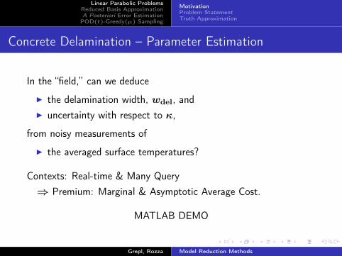
Concrete Delamination – Parameter Estimation
In the “field,” can we deduce
I the delamination width, wdel, andI uncertainty with respect to κ,
from noisy measurements of
I the averaged surface temperatures?
Contexts: Real-time & Many Query⇒ Premium: Marginal & Asymptotic Average Cost.
MATLAB DEMO
Grepl, Rozza Model Reduction Methods

Linear Parabolic ProblemsReduced Basis ApproximationA Posteriori Error EstimationPOD(t)-Greedy(µ) Sampling
MotivationProblem StatementTruth Approximation
Reduced Basis Methods for Time-dependent Problems
New ingredients/challenges:
I Simultaneous dependence on both time and parameters.I "Time" as an additional (albeit special) parameter.
I Output, s = s(t;µ), is a function of time (and parameter).I Important for applications, e.g., control.I A posteriori error bounds (no "compliance"⇒ dual problem).
I Sampling procedure.I Greedy algorithm for parameter-time case.I Unknown "control" input.
I Dimension N of RB space.I Advection-dominated problems.
Grepl, Rozza Model Reduction Methods

Linear Parabolic ProblemsReduced Basis ApproximationA Posteriori Error EstimationPOD(t)-Greedy(µ) Sampling
MotivationProblem StatementTruth Approximation
Problem Statement
Given µ ∈ D ⊂ RP , evaluate t ∈ (0, tf ]
se(t;µ) = `(ue(x; t;µ);µ)
where ue(x; t;µ) ∈ L2(0, tf ;Xe(Ω)) satisfies u0 = 0
m
(∂ue
∂t(x; t;µ), v;µ
)+ a(ue(x; t;µ), v;µ)
= f(v;µ) g(t), ∀ v ∈ Xe.
Note: For now, we assume u0 = 0 – extension to nonzero initialconditions are briefly discussed below.
Grepl, Rozza Model Reduction Methods

Linear Parabolic ProblemsReduced Basis ApproximationA Posteriori Error EstimationPOD(t)-Greedy(µ) Sampling
MotivationProblem StatementTruth Approximation
Definitions
µ: input parameter - µ = (µ1, µ2, . . . , µP ); P -tuple
D: parameter domain in RP ;
Ω: spatial domain in Rd;
se: output;
`: output functional;
ue: field variable;
Xe: function space (H10(Ω))ν ⊂ Xe ⊂ (H1(Ω))ν †,
with inner product (w, v)Xe, ∀w, v ∈ Xe,
and induced norm ‖w‖Xe =√
(w,w)Xe, ∀w ∈ Xe.† For simplicity we assume ν = 1.
Grepl, Rozza Model Reduction Methods

Linear Parabolic ProblemsReduced Basis ApproximationA Posteriori Error EstimationPOD(t)-Greedy(µ) Sampling
MotivationProblem StatementTruth Approximation
Reference Geometry
Note Ω is parameter-independent:
I the reduced basis requires a common spatial configuration, i.e.,a reference domain Ωref
I Introduce a piecewise affine mapping T (·;µ) : Ω→ Ωo(µ)
ao(wo, vo;µ) over Ωo(µ)⇓
T (·;µ)−1 : Ωo(µ)→ Ωref ≡ Ω⇓
a(w, v;µ) over Ω
(Ωref = Ωo(µref))
where a(w, v;µ) = ao(wo Tµ, vo Tµ;µ)
We henceforth assume that the problem is already mapped to thereference domain.
Grepl, Rozza Model Reduction Methods

Linear Parabolic ProblemsReduced Basis ApproximationA Posteriori Error EstimationPOD(t)-Greedy(µ) Sampling
MotivationProblem StatementTruth Approximation
Hypotheses
Linear forms and functions
f(·;µ) : linear, affine in µ,Xe-bounded, ∀µ ∈ D
g(·) : L2(0, tf) “control” input
`(·;µ) : linear, affine in µ,L2(Ω)-bounded, ∀µ ∈ D
Grepl, Rozza Model Reduction Methods

Linear Parabolic ProblemsReduced Basis ApproximationA Posteriori Error EstimationPOD(t)-Greedy(µ) Sampling
MotivationProblem StatementTruth Approximation
Hypotheses
a(·, ·;µ) : bilinear, affine in µ,symmetric,Xe-continuous,Xe-coercive form, ∀µ ∈ D;
m(·, ·;µ) : bilinear, affine in µ,symmetric,L2(Ω)-continuous,L2(Ω)-coercive form, ∀µ ∈ D;
Extensions to non-symmetric, non-affine, non-linear are possible . . .. . . and are partly discussed later on.
Grepl, Rozza Model Reduction Methods

Linear Parabolic ProblemsReduced Basis ApproximationA Posteriori Error EstimationPOD(t)-Greedy(µ) Sampling
MotivationProblem StatementTruth Approximation
Affine parameter dependence
Require also `(v;µ), f(v;µ)
a(w, v;µ) =Qa∑q=1
Θqa(µ) aq(w, v),
m(w, v;µ) =Qm∑q=1
Θqm(µ) mq(w, v);
whereΘqa,m : D → R, µ-dependent functions;
representing coefficients, geometry, . . .
aq and mq µ-independent forms.
Note: affine assumption may be relaxed [BMNP,GMNP].
Grepl, Rozza Model Reduction Methods

Linear Parabolic ProblemsReduced Basis ApproximationA Posteriori Error EstimationPOD(t)-Greedy(µ) Sampling
MotivationProblem StatementTruth Approximation
Truth Approximation
I Spatial Discretization: Finite Element
XN ⊂ X with dim(XN ) = N
for given N (N →∞).We may also consider Finite Volume [HO]
I Temporal Discretization: Finite Difference
tk = k∆t, ∀k ∈ K ≡ (0), 1, 2, . . . ,K
for given ∆t = tf/K (fixed).We may also consider DG [RMM]
Grepl, Rozza Model Reduction Methods

Linear Parabolic ProblemsReduced Basis ApproximationA Posteriori Error EstimationPOD(t)-Greedy(µ) Sampling
MotivationProblem StatementTruth Approximation
Truth Approximation
I Temporal Discretization: Finite Difference
∂u
∂t(tk;µ) ≈
u(tk;µ)− u(tk−1;µ)
∆t
I Euler BackwardI Crank-Nicolson (advection-dominated problems)
∆t ∆t
t1 = ∆t
∆t
t2 = 2∆t tK = K∆t = tft0 = 0
s(t1;µ)s(t2;µ) s(tK;µ)
s(t0;µ)
Grepl, Rozza Model Reduction Methods

Linear Parabolic ProblemsReduced Basis ApproximationA Posteriori Error EstimationPOD(t)-Greedy(µ) Sampling
MotivationProblem StatementTruth Approximation
Problem Statement
Given µ ∈ D ⊂ RP , evaluate ∀k ∈ K
sk(µ) ≡ s(tk;µ) = `(u(tk;µ);µ)
where uk(µ) ≡ u(tk;µ) ∈ X satisfies u0 = 0
m
(u(tk;µ)− u(tk−1;µ)
∆t, v;µ
)+ a(u(tk;µ), v;µ)
= f(v;µ) g(tk), ∀ v ∈ X.
Note: We directly drop the superscript N , i.e., X = XN ,
u(tk;µ) = uN (tk;µ), s(tk;µ) = sN (tk;µ).
Grepl, Rozza Model Reduction Methods
Linear Parabolic ProblemsReduced Basis ApproximationA Posteriori Error EstimationPOD(t)-Greedy(µ) Sampling
MotivationProblem StatementTruth Approximation
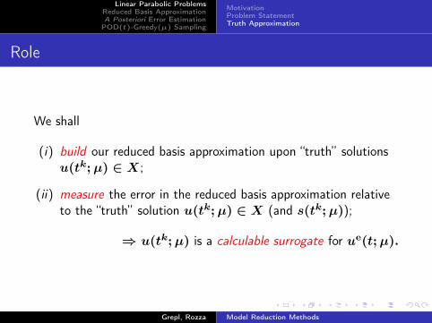
Role
We shall
(i) build our reduced basis approximation upon “truth” solutionsu(tk;µ) ∈ X;
(ii) measure the error in the reduced basis approximation relativeto the “truth” solution u(tk;µ) ∈ X (and s(tk;µ));
⇒ u(tk;µ) is a calculable surrogate for ue(t;µ).
Grepl, Rozza Model Reduction Methods

Linear Parabolic ProblemsReduced Basis ApproximationA Posteriori Error EstimationPOD(t)-Greedy(µ) Sampling
RB Spaces & BasesApproximationOfline-Online ProcedureAlgebraic Equations
Parametric ManifoldMNK
We assume
I the form a is continuous and coercive (or inf-sup stable); andI the form m is continuous and coercive; andI the Θq
m,a(µ), 1 ≤ q ≤ Qm,a, are smooth;
then
MNK ≡ u(tk;µ) | 1 ≤ k ≤ K, ∀µ ∈ D
lies on a smooth P + 1-dimensional manifold in X.
Grepl, Rozza Model Reduction Methods

Linear Parabolic ProblemsReduced Basis ApproximationA Posteriori Error EstimationPOD(t)-Greedy(µ) Sampling
RB Spaces & BasesApproximationOfline-Online ProcedureAlgebraic Equations
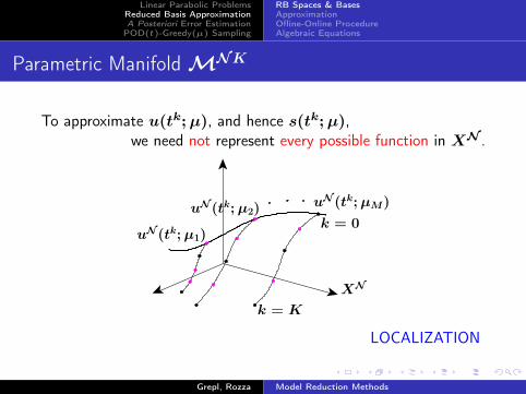
Parametric ManifoldMNK
To approximate u(tk;µ), and hence s(tk;µ),we need not represent every possible function in XN .
k = K
k = 0uN(tk;µ1)
uN(tk;µ2)uN(tk;µM)
XN
XN ⊂ spanu(tk;µm), 1 ≤ k ≤ K, 1 ≤ m ≤M;
Grepl, Rozza Model Reduction Methods
Linear Parabolic ProblemsReduced Basis ApproximationA Posteriori Error EstimationPOD(t)-Greedy(µ) Sampling
RB Spaces & BasesApproximationOfline-Online ProcedureAlgebraic Equations
Parametric ManifoldMNK
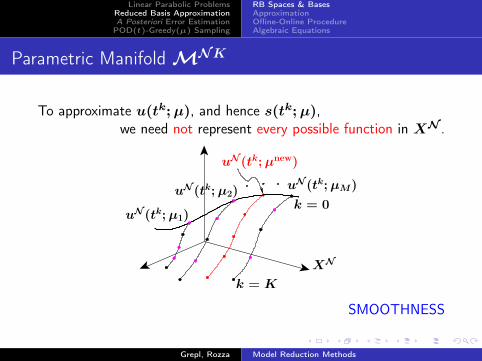
To approximate u(tk;µ), and hence s(tk;µ),we need not represent every possible function in XN .
k = K
k = 0
XN
uN(tk;µ1)
uN(tk;µ2)uN(tk;µM)
LOCALIZATION
Grepl, Rozza Model Reduction Methods
Linear Parabolic ProblemsReduced Basis ApproximationA Posteriori Error EstimationPOD(t)-Greedy(µ) Sampling
RB Spaces & BasesApproximationOfline-Online ProcedureAlgebraic Equations
Parametric ManifoldMNK
To approximate u(tk;µ), and hence s(tk;µ),we need not represent every possible function in XN .
k = K
k = 0
XN
uN(tk;µ1)
uN(tk;µ2)
uN(tk;µnew)
uN(tk;µM)
SMOOTHNESS
Grepl, Rozza Model Reduction Methods

Linear Parabolic ProblemsReduced Basis ApproximationA Posteriori Error EstimationPOD(t)-Greedy(µ) Sampling
RB Spaces & BasesApproximationOfline-Online ProcedureAlgebraic Equations
Reduced Basis Space
We define the Lagrangian RB space
XN = spanζn, 1 ≤ n ≤ N, 1 ≤ N ≤ Nmax,
with mutually (·, ·)X -orthonormal basis functions
ζn ∈ X, 1 ≤ n ≤ Nmax.
We thus obtainXN ⊂ X, dim(XN) = N, 1 ≤ N ≤ Nmax,
and hierarchical spacesX1 ⊂ X2 ⊂ . . . ⊂ XNmax−1 ⊂ XNmax(⊂ X).
The basis functions are constructed using a POD-Greedy algorithmoutlined below.
Grepl, Rozza Model Reduction Methods

Linear Parabolic ProblemsReduced Basis ApproximationA Posteriori Error EstimationPOD(t)-Greedy(µ) Sampling
RB Spaces & BasesApproximationOfline-Online ProcedureAlgebraic Equations
Galerkin Projection
Given µ ∈ D ⊂ RP , evaluate ∀k ∈ K
skN(µ) ≡ sN(tk;µ) = `(uN(tk;µ);µ)
where ukN(µ) ≡ uN(tk;µ) ∈ XN satisfies uN,0 = 0
m
(uN(tk;µ)− uN(tk−1;µ)
∆t, v;µ
)+ a(uN(tk;µ), v;µ)
= f(v;µ) g(tk), ∀ v ∈ XN .
⇒ reduced basis inherits the fixed truth temporal discretization.
Grepl, Rozza Model Reduction Methods

Linear Parabolic ProblemsReduced Basis ApproximationA Posteriori Error EstimationPOD(t)-Greedy(µ) Sampling
RB Spaces & BasesApproximationOfline-Online ProcedureAlgebraic Equations
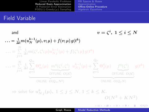
Field Variable
We expand ukN(µ) =N∑j=1
ukN j(µ)ζj
and obtain v = ζi, 1 ≤ i ≤ N
a(ukN(µ), v;µ) + 1∆tm(ukN(µ), v;µ) = . . .
N∑j=1
[a(ζj, ζi;µ) + 1
∆tm(ζj, ζi;µ)
]ukN j(µ) = . . .
N∑j=1
[ Qa∑q=1
Θqa(µ) aq(ζj, ζi)︸ ︷︷ ︸
OFFLINE: O(N )︸ ︷︷ ︸ONLINE: O(QaN2)
+ 1∆t
Qm∑q=1
Θqm(µ) mq(ζj, ζi)︸ ︷︷ ︸
OFFLINE: O(N )︸ ︷︷ ︸ONLINE: O(QmN2)
]ukN j(µ) = . . .
Grepl, Rozza Model Reduction Methods

Linear Parabolic ProblemsReduced Basis ApproximationA Posteriori Error EstimationPOD(t)-Greedy(µ) Sampling
RB Spaces & BasesApproximationOfline-Online ProcedureAlgebraic Equations
Field Variable
We expand ukN(µ) =N∑j=1
ukN j(µ)ζj
and obtain v = ζi, 1 ≤ i ≤ N
a(ukN(µ), v;µ) + 1∆tm(ukN(µ), v;µ) = . . .
N∑j=1
[a(ζj, ζi;µ) + 1
∆tm(ζj, ζi;µ)
]ukN j(µ) = . . .
N∑j=1
[ Qa∑q=1
Θqa(µ) aq(ζj, ζi)︸ ︷︷ ︸
OFFLINE: O(N )︸ ︷︷ ︸ONLINE: O(QaN2)
+ 1∆t
Qm∑q=1
Θqm(µ) mq(ζj, ζi)︸ ︷︷ ︸
OFFLINE: O(N )︸ ︷︷ ︸ONLINE: O(QmN2)
]ukN j(µ) = . . .
Grepl, Rozza Model Reduction Methods
Linear Parabolic ProblemsReduced Basis ApproximationA Posteriori Error EstimationPOD(t)-Greedy(µ) Sampling
RB Spaces & BasesApproximationOfline-Online ProcedureAlgebraic Equations
Field Variable
and v = ζi, 1 ≤ i ≤ N
. . . = 1∆tm(uk−1
N (µ), v;µ) + f(v;µ) g(tk)
. . . =N∑j=1
1∆tm(ζj, ζi;µ)uk−1
N j (µ) + f(ζi;µ) g(tk)
. . . =N∑j=1
1∆t
Qm∑q=1
Θqm(µ) mq(ζj, ζi)︸ ︷︷ ︸
OFFLINE: O(N )︸ ︷︷ ︸ONLINE: O(QmN2)
uk−1N j (µ) +
Qf∑q=1
Θqf(µ) fq(ζi)︸ ︷︷ ︸
OFFLINE: O(N )︸ ︷︷ ︸ONLINE: O(QfN)
g(tk)
⇒ solve for ukN j(µ), 1 ≤ j ≤ N , 1 ≤ k ≤ K.O(N3 +KN2)
Grepl, Rozza Model Reduction Methods
Linear Parabolic ProblemsReduced Basis ApproximationA Posteriori Error EstimationPOD(t)-Greedy(µ) Sampling
RB Spaces & BasesApproximationOfline-Online ProcedureAlgebraic Equations
Output Evaluation
Given ukN j(µ), 1 ≤ j ≤ N , evaluate the output from ∀k ∈ K
skN(µ) = `(ukN(µ);µ) =N∑j=1
ukN j(µ)`(ζj;µ)
=N∑j=1
ukN j(µ)Q∑q=1
Θq`(µ) `q(ζj)︸ ︷︷ ︸
OFFLINE: O(N )︸ ︷︷ ︸ONLINE: O(Q`N)︸ ︷︷ ︸
ONLINE: O(N)
⇒ solve for skN(µ), 1 ≤ k ≤ K, in O(KN).
Grepl, Rozza Model Reduction Methods

Linear Parabolic ProblemsReduced Basis ApproximationA Posteriori Error EstimationPOD(t)-Greedy(µ) Sampling
RB Spaces & BasesApproximationOfline-Online ProcedureAlgebraic Equations
Computational Cost
Summary computational cost: (Q = Qa +Qm)
OFFLINE — once, parameter independent
O(KNmaxN •) + O(QN2maxN )
solve for ζn form µ-independent quantities;
ONLINE — many times, parameter dependent µnew
O(QN2) + O(N3 +KN2) + O(KN)form RB matrices solve for ukNj(µ) evaluate output
;
Online cost is independent of N .
Grepl, Rozza Model Reduction Methods

Linear Parabolic ProblemsReduced Basis ApproximationA Posteriori Error EstimationPOD(t)-Greedy(µ) Sampling
RB Spaces & BasesApproximationOfline-Online ProcedureAlgebraic Equations
Stiffness Matrix
Evaluation of RB Stiffness Matrix AN ∈ RN×N :
Parameter-independent matrices AqN ∈ RN×N , 1 ≤ q ≤ Qa:
AqN nm = aq(ζm, ζn)
=N∑i=1
N∑j=1
ζmi aq(ϕNi , ϕNj ) ζnj , 1 ≤ n,m ≤ N,
thusAqN = ZTN ANq ZN .
We finally assemble
AN =Qa∑q=1
Θqa(µ) AqN .
Here, ZN = [ζ1 ζ2 . . . ζN ] ∈ RN×N .
Grepl, Rozza Model Reduction Methods
Linear Parabolic ProblemsReduced Basis ApproximationA Posteriori Error EstimationPOD(t)-Greedy(µ) Sampling
RB Spaces & BasesApproximationOfline-Online ProcedureAlgebraic Equations
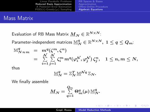
Mass Matrix
Evaluation of RB Mass Matrix MN ∈ RN×N :
Parameter-independent matrices MqN ∈ RN×N , 1 ≤ q ≤ Qm:
MqN nm = mq(ζm, ζn)
=N∑i=1
N∑j=1
ζmi mq(ϕNi , ϕNj ) ζnj , 1 ≤ n,m ≤ N,
thusMqN = ZTN MNq ZN .
We finally assemble
MN =Qm∑q=1
Θqm(µ) Mq
N .
Grepl, Rozza Model Reduction Methods

Linear Parabolic ProblemsReduced Basis ApproximationA Posteriori Error EstimationPOD(t)-Greedy(µ) Sampling
RB Spaces & BasesApproximationOfline-Online ProcedureAlgebraic Equations
Load/Source Vector
Evaluation of RB Load/Source Vector FN ∈ RN :
Parameter-independent vectors FqN ∈ RN , 1 ≤ q ≤ Qf :
FqN n = fq(ζn)
=N∑i=1
ζmi fq(ϕNi ), 1 ≤ n ≤ N,
thusFqN = ZTN FNq.
We finally assemble
FN =Qf∑q=1
Θqf(µ) FqN .
Grepl, Rozza Model Reduction Methods

Linear Parabolic ProblemsReduced Basis ApproximationA Posteriori Error EstimationPOD(t)-Greedy(µ) Sampling
RB Spaces & BasesApproximationOfline-Online ProcedureAlgebraic Equations
Output Vector
Evaluation of RB Output Vector LN ∈ RN :
Parameter-independent vectors LqN ∈ RN , 1 ≤ q ≤ Q`:
LqN n = `q(ζn)
=N∑i=1
ζmi `q(ϕNi ), 1 ≤ n ≤ N,
thusLqN = ZTN LNq.
We finally assemble
LN =Q∑q=1
Θq`(µ) LqN .
Grepl, Rozza Model Reduction Methods

Linear Parabolic ProblemsReduced Basis ApproximationA Posteriori Error EstimationPOD(t)-Greedy(µ) Sampling
RB Spaces & BasesApproximationOfline-Online ProcedureAlgebraic Equations
Summary
Given µ ∈ D, evaluate ∀k ∈ K
skN(µ) = LTN(µ)ukN(µ)
where ukN(µ) ∈ RN satisfies uN,0(µ) = 0(AN(µ) + 1
∆tMN(µ)
)ukN(µ) =
1∆tMN(µ)uk−1
N (µ) + FN(µ) g(tk).
I LU-decomposition: AN(µ) + 1∆tMN(µ)
I Forward/Back Substitution: ukN(µ), ∀k ∈ KArrays for N ≤ Nmax are principal subarrays of arrays for N = Nmax.
Grepl, Rozza Model Reduction Methods

Linear Parabolic ProblemsReduced Basis ApproximationA Posteriori Error EstimationPOD(t)-Greedy(µ) Sampling
RB Spaces & BasesApproximationOfline-Online ProcedureAlgebraic Equations
Example: Concrete Delamination – Results
Delamination
Heat Flux
FRP laminate
q(t)
x1
Concrete slab
x2
κ
ΓF
wdel
Ω2 , Measurement 2
Γdel
, Measurement 1Ω1
Ω0,FRP%FRP, cP,FRP, kFRP
Ω0,C%C, cP,C, kC 1 [kC]
y0(x, t = 0;µ) = 0
Input (parameter): µ ≡ (wdel/2, κ ≡ kFRP/kC) ⊂ D,where D ≡ [1, 10]× [0.4, 1.8].
“Truth”: N = 5601, K = 200.
Grepl, Rozza Model Reduction Methods

Linear Parabolic ProblemsReduced Basis ApproximationA Posteriori Error EstimationPOD(t)-Greedy(µ) Sampling
RB Spaces & BasesApproximationOfline-Online ProcedureAlgebraic Equations
Example: Concrete Delamination – Results
N εumax,rel εsmax,rel
20 8.09E –02 6.76E –0140 2.71E –02 1.44E –0260 1.02E –02 3.34E –0380 5.02E –03 1.43E –03120 7.40E –04 9.81E –05160 2.13E –04 2.34E –05200 9.55E –05 6.02E –06
I Maximum relative error:εumax,rel = max
µ∈Ξtest
|||eK |||µ|||uK(µ)||| , µu = arg max
µ∈Ξtest
|||uK(µ)|||
I Maximum relative output error:εsmax,rel = max
µ∈Ξtest
maxk∈K
|sk(µ)−skN (µ)|smax
, smax = maxµ∈Ξtest
maxk∈K|sk(µ)|
How do we choose N?Grepl, Rozza Model Reduction Methods

Linear Parabolic ProblemsReduced Basis ApproximationA Posteriori Error EstimationPOD(t)-Greedy(µ) Sampling
PreliminariesPrimal-only FormualationPrimal-Dual FormulationNumerical Results
Motivation
How do we know that ukN(µ), skN(µ) are accurate? ONLINE
|||uk(µ)− ukN(µ)|||µ ≤ εtol,min, ∀k ∈ K, ∀µ ∈ D
|sk(µ)− skN(µ)| ≤ εstol,min, ∀k ∈ K, ∀µ ∈ D
How do we know what value of N to take? ONLINE/OFFLINE
N too large ⇒ computational inefficiencyN too small ⇒ unacceptable uncertainty
How do we choose the sample SN optimally? OFFLINE
RB space has to approximate manifoldM well, butRB matrices need to be “well-conditioned.”
Grepl, Rozza Model Reduction Methods

Linear Parabolic ProblemsReduced Basis ApproximationA Posteriori Error EstimationPOD(t)-Greedy(µ) Sampling
PreliminariesPrimal-only FormualationPrimal-Dual FormulationNumerical Results
Requirements
Our a posteriori error bounds, ∆kN(µ) and ∆s k
N (µ), must be
I rigorous 1 ≤ N ≤ Nmax
|||uk(µ)− ukN(µ)||| ≤ ∆N(µ), ∀k ∈ K, ∀µ ∈ D,|sk(µ)− skN(µ)| ≤ ∆s
N(µ), ∀k ∈ K, ∀µ ∈ D.
I reasonably sharp
∆kN(µ)
|||uk(µ)− ukN(µ)|||≤ C,
∆s kN (µ)
|sk(µ)− skN(µ)|≤ C,
where C ≈ 1.I efficient
⇒ Online cost depends on N , Q, and K, but not on N .
Grepl, Rozza Model Reduction Methods
Linear Parabolic ProblemsReduced Basis ApproximationA Posteriori Error EstimationPOD(t)-Greedy(µ) Sampling
PreliminariesPrimal-only FormualationPrimal-Dual FormulationNumerical Results
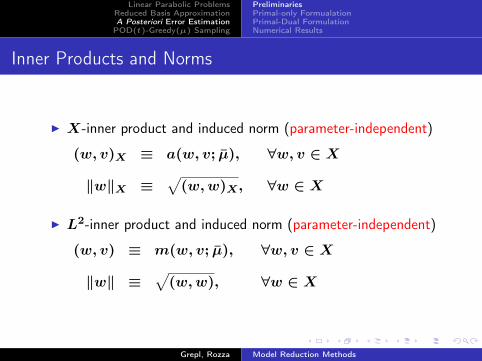
Inner Products and Norms
I X-inner product and induced norm (parameter-independent)
(w, v)X ≡ a(w, v; µ), ∀w, v ∈ X
‖w‖X ≡√
(w,w)X , ∀w ∈ X
I L2-inner product and induced norm (parameter-independent)
(w, v) ≡ m(w, v; µ), ∀w, v ∈ X
‖w‖ ≡√
(w,w), ∀w ∈ X
Grepl, Rozza Model Reduction Methods

Linear Parabolic ProblemsReduced Basis ApproximationA Posteriori Error EstimationPOD(t)-Greedy(µ) Sampling
PreliminariesPrimal-only FormualationPrimal-Dual FormulationNumerical Results
Inner Products and Norms
I “Spatio-temporal” energy norm (parameter-dependent)
(((wk, vk))) = m(wk, vk;µ)
+k∑
k′=1
∆t a(wk′, vk
′;µ),
|||wk||| =(m(wk, wk;µ)
+k∑
k′=1
∆t a(wk′, wk
′;µ)
)1/2
,
1 ≤ k ≤ K.
Grepl, Rozza Model Reduction Methods

Linear Parabolic ProblemsReduced Basis ApproximationA Posteriori Error EstimationPOD(t)-Greedy(µ) Sampling
PreliminariesPrimal-only FormualationPrimal-Dual FormulationNumerical Results
Coercivity and Continuity constants
We also define
I Coercivity constants
α(µ) ≡ infw∈X
a(w,w;µ)
‖w‖2X; σ(µ) ≡ inf
w∈X
m(w,w;µ)
‖w‖2;
I Continuity constants
γa(µ) ≡ supw∈X
supv∈X
a(w, v;µ)
‖w‖X‖v‖X.
γm(µ) ≡ supw∈X
supv∈X
m(w, v;µ)
‖w‖ ‖v‖.
Grepl, Rozza Model Reduction Methods

Linear Parabolic ProblemsReduced Basis ApproximationA Posteriori Error EstimationPOD(t)-Greedy(µ) Sampling
PreliminariesPrimal-only FormualationPrimal-Dual FormulationNumerical Results
Coercivity Lower Bound
We require a positive lower bound for the coercivity constant
I αLB : D → R0 < αLB(µ) ≤ α(µ), ∀µ ∈ D.
I σLB : D → R0 < σLB(µ) ≤ σ(µ), ∀µ ∈ D.
This bound can be calculated using the
I “min Θ” Approach (if a is parametrically coercive), orI Successive Constraint Method [HRSP]
exactly as in elliptic case.
Grepl, Rozza Model Reduction Methods

Linear Parabolic ProblemsReduced Basis ApproximationA Posteriori Error EstimationPOD(t)-Greedy(µ) Sampling
PreliminariesPrimal-only FormualationPrimal-Dual FormulationNumerical Results
Dual Norm of Residual
We define the residual, ∀k ∈ K,
rk(v;µ) ≡ f(v;µ) g(tk)−m(uN (tk;µ)−uN (tk−1;µ)
∆t, v;µ
)−a(uN(tk;µ), v;µ), ∀ v ∈ X
Dual Norm of Residual
Given µ ∈ D, the dual norm of rk(v;µ) is defined as
‖rk(·;µ)‖X′ ≡ supv∈X
rk(v;µ)
‖v‖X= ‖ek(µ)‖X ,
where ek(µ) ∈ X satisfies(ek(µ), v)X = rk(v;µ), ∀v ∈ X.
Grepl, Rozza Model Reduction Methods

Linear Parabolic ProblemsReduced Basis ApproximationA Posteriori Error EstimationPOD(t)-Greedy(µ) Sampling
PreliminariesPrimal-only FormualationPrimal-Dual FormulationNumerical Results
Energy Error Bound
We define the error bound, ∆kN(µ) = ∆N(tk;µ), 1 ≤ k ≤ K,
as
∆kN(µ) = α
−1/2LB (µ)
(k∑
k′=1
∆t ‖ek′(µ)‖2X
)1/2
.
We can then prove
Proposition (Energy Error Bound)
For any N = 1, . . . , Nmax, the error in the field variable,ek(µ) = uk(µ)− ukN(µ), is bounded by
|||ek(µ)||| ≤ ∆kN(µ), ∀ µ ∈ D, ∀ k ∈ K.
Grepl, Rozza Model Reduction Methods

Linear Parabolic ProblemsReduced Basis ApproximationA Posteriori Error EstimationPOD(t)-Greedy(µ) Sampling
PreliminariesPrimal-only FormualationPrimal-Dual FormulationNumerical Results
Energy Error Bound
Proof.
Sketch: The error, ek(µ) = uk(µ)− ukN(µ), satisfies
m(ek(µ)−ek−1(µ)
∆t, v;µ
)+ a(ek(µ), v;µ)
= rk(v;µ), ∀ v ∈ X, ∀ k ∈ K.We now choose v = ek(µ) and apply
I Cauchy-Schwarz to m(ek−1(µ), ek(µ);µ),I the definition of the dual norm of the residual,I Young’s Inequality (twice): for c ∈ R, d ∈ R, ρ ∈ R+
2|c| |d| ≤ 1ρ2 c
2 + ρ2d2
I and finally sum from k′ = 1 to k.
Grepl, Rozza Model Reduction Methods

Linear Parabolic ProblemsReduced Basis ApproximationA Posteriori Error EstimationPOD(t)-Greedy(µ) Sampling
PreliminariesPrimal-only FormualationPrimal-Dual FormulationNumerical Results
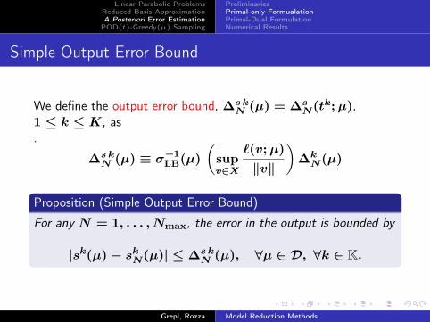
Simple Output Error Bound
We define the output error bound, ∆s kN (µ) = ∆s
N(tk;µ),1 ≤ k ≤ K, as.
∆s kN (µ) ≡ σ−1
LB(µ)(
supv∈X
`(v;µ)
‖v‖
)∆kN(µ)
Proposition (Simple Output Error Bound)
For any N = 1, . . . , Nmax, the error in the output is bounded by
|sk(µ)− skN(µ)| ≤ ∆s kN (µ), ∀µ ∈ D, ∀k ∈ K.
Grepl, Rozza Model Reduction Methods
Linear Parabolic ProblemsReduced Basis ApproximationA Posteriori Error EstimationPOD(t)-Greedy(µ) Sampling
PreliminariesPrimal-only FormualationPrimal-Dual FormulationNumerical Results
Simple Output Error Bound
We define the output error bound, ∆s kN (µ) = ∆s
N(tk;µ),1 ≤ k ≤ K, as.
∆s kN (µ) ≡ σ−1
LB(µ)(
supv∈X
`(v;µ)
‖v‖
)∆kN(µ)
Proposition (Simple Output Error Bound)
For any N = 1, . . . , Nmax, the error in the output is bounded by
|sk(µ)− skN(µ)| ≤ ∆s kN (µ), ∀µ ∈ D, ∀k ∈ K.
Grepl, Rozza Model Reduction Methods

Linear Parabolic ProblemsReduced Basis ApproximationA Posteriori Error EstimationPOD(t)-Greedy(µ) Sampling
PreliminariesPrimal-only FormualationPrimal-Dual FormulationNumerical Results
Error Bounds
Remarks:
I The error bounds are rigorous upper bounds for the reducedbasis error for any N = 1, . . . , Nmax, for all µ ∈ D, and forall k ∈ K.
I Define: s±N(tk;µ) = sN(tk;µ)±∆s(tk;µ), then
⇒ s−N(tk;µ) ≤ s(tk;µ) ≤ s+N(tk;µ)
I We may also consider other norms than ||| · |||, i.e., L2(Ω)[HO].
Grepl, Rozza Model Reduction Methods

Linear Parabolic ProblemsReduced Basis ApproximationA Posteriori Error EstimationPOD(t)-Greedy(µ) Sampling
PreliminariesPrimal-only FormualationPrimal-Dual FormulationNumerical Results
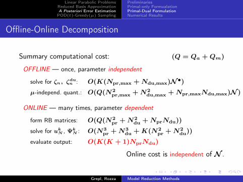
Offline-Online Decomposition
Crucial ingredient: Dual norm of residual ‖ek(µ)‖X , ∀k ∈ K.
Computational procedure follows directly from the elliptic case withadded complexity due to mass term and time dependence.
I Expand uN(µ) =N∑j=1
ukN j(µ) ζj
I Riesz representation:(ek(µ), v)X = rk(v;µ)
I Affine decomposition
I Linear superposition
Grepl, Rozza Model Reduction Methods

Linear Parabolic ProblemsReduced Basis ApproximationA Posteriori Error EstimationPOD(t)-Greedy(µ) Sampling
PreliminariesPrimal-only FormualationPrimal-Dual FormulationNumerical Results
Offline-Online Decomposition
Summary of computational cost: Q = Qa +Qm
OFFLINE —
O(QNmaxN •) + O(Q2N2maxN )
solve Poisson problems form µ-independent inner products;
ONLINE —
O(KQ2N2)evaluate ‖ek(µ)‖X -sum for 1 ≤ k ≤ K
;
Online cost is independent of N .
Grepl, Rozza Model Reduction Methods

Linear Parabolic ProblemsReduced Basis ApproximationA Posteriori Error EstimationPOD(t)-Greedy(µ) Sampling
PreliminariesPrimal-only FormualationPrimal-Dual FormulationNumerical Results
Example: Concrete Delamination – Results
Convergence energy norm error and boundN εumax,rel ∆u
max,rel ηu
20 8.09E –02 3.18E –01 2.7440 2.71E –02 8.01E –02 2.7760 1.02E –02 2.01E –02 2.5880 5.02E –03 8.40E –03 2.83120 7.40E –04 1.71E –03 2.45160 2.13E –04 4.84E –04 2.21200 9.55E –05 2.70E –04 2.20
I Maximum relative error bound:∆y
max,rel = maxµ∈Ξtest
∆kN (µ)
|||uK(µ)||| , µu = arg maxµ∈Ξtest
|||uK(µ)|||
I Average effectivity:ηu = 1
ntrainK
Pµ∈Ξtest
Pk∈K
∆kN (µ)
|||ek(µ)|||
Grepl, Rozza Model Reduction Methods

Linear Parabolic ProblemsReduced Basis ApproximationA Posteriori Error EstimationPOD(t)-Greedy(µ) Sampling
PreliminariesPrimal-only FormualationPrimal-Dual FormulationNumerical Results
Example: Concrete Delamination – Results
Convergence output error and boundN εsmax,rel ∆s
max,rel ηs
20 6.76E –02 2.58E+01 21140 1.44E –02 6.24E+00 34160 3.34E –03 1.46E+00 36380 1.43E –03 4.73E –01 379120 9.81E –05 1.24E –01 604160 2.34E –05 2.88E –02 674200 6.02E –06 9.18E –03 1117
I Maximum relative output bound:∆s
max,rel = maxµ∈Ξtest
∆sKN (µ)
|smax|
I Average output effectivity:
ηs = 1ntrain
Pµ∈Ξtest
∆s kη(µ)
N (µ)
|skη(µ)(µ)−skη(µ)
N (µ)|, kη(µ) = arg max
k∈K|sk(µ)− skN(µ)|
Grepl, Rozza Model Reduction Methods

Linear Parabolic ProblemsReduced Basis ApproximationA Posteriori Error EstimationPOD(t)-Greedy(µ) Sampling
PreliminariesPrimal-only FormualationPrimal-Dual FormulationNumerical Results
Motivation
The notion “compliance” does not exist in the parabolic context.Thus similar to the noncompliant elliptic problem, we consider aprimal-dual formulation for the parabolic problem
Goal:I Faster convergence of output error & bound.
output error = primal error(Npr) × dual error(Ndu)
I Improved effectivities for output error estimation.
Grepl, Rozza Model Reduction Methods

Linear Parabolic ProblemsReduced Basis ApproximationA Posteriori Error EstimationPOD(t)-Greedy(µ) Sampling
PreliminariesPrimal-only FormualationPrimal-Dual FormulationNumerical Results
Dual Problem
Introduce dual problem for output at time t′:
Given µ ∈ D, the dual variable ψe(t;µ), 0 < t ≤ t′, satisfies
m(v, ∂ψ
e
∂t(t;µ);µ
)− a(v, ψe(t;µ);µ) = 0, ∀v ∈ Xe
with final condition
m(v, ψe(t′;µ);µ) ≡ l(v;µ), ∀v ∈ Xe.
Note that the dual problem evolves backward in time with finalcondition defined at the "time of interest."
Grepl, Rozza Model Reduction Methods

Linear Parabolic ProblemsReduced Basis ApproximationA Posteriori Error EstimationPOD(t)-Greedy(µ) Sampling
PreliminariesPrimal-only FormualationPrimal-Dual FormulationNumerical Results
Dual Problem – Truth Approximation
FD[t] – FE Galerkin[x] Truth Approximation:I EB or CN: ∆t = tf/K, t
k = k∆t, 0 ≤ k ≤ KI ψ(tk;µ) = ψN (tk;µ) ∈ XN ⊂ Xe, dim(XN ) = N
⇒ inherited from primal problem.
Introduce truth dual problem for output at time tL, 1 ≤ L ≤ K:
Given µ ∈ D, the dual variable ψL(tk;µ), 1 ≤ k ≤ L, satisfies
m(v, ψ
L(tk;µ)−ψL(tk+1;µ)∆t
;µ)− a(v, ψL(tk;µ);µ) = 0, ∀v ∈ X,
with final condition
m(v, ψL(tL;µ);µ) ≡ l(v;µ), ∀v ∈ X.
Grepl, Rozza Model Reduction Methods

Linear Parabolic ProblemsReduced Basis ApproximationA Posteriori Error EstimationPOD(t)-Greedy(µ) Sampling
PreliminariesPrimal-only FormualationPrimal-Dual FormulationNumerical Results
Dual Problem – LTI Property
Invoking the LTI (linear time-invariance) property we can expressthe dual for the output at time tL, 1 ≤ L ≤ K, as
ψL(tk;µ) ≡ Ψ(tK−L+k;µ), 1 ≤ k ≤ L,
where Ψ(tk;µ), 1 ≤ k ≤ K evolves backward from the finaltime tK .
⇒ To obtain ψL(tk;µ), 1 ≤ k ≤ L, 1 ≤ L ≤ K, weI solve once for Ψk(tk;µ), 1 ≤ k ≤ K, and thenI appropriately shift the result
— we do not need to solve K dual problems.
Note: shifting property does not hold for LTV systems.
Grepl, Rozza Model Reduction Methods

Linear Parabolic ProblemsReduced Basis ApproximationA Posteriori Error EstimationPOD(t)-Greedy(µ) Sampling
PreliminariesPrimal-only FormualationPrimal-Dual FormulationNumerical Results
Dual Problem – LTI Property
t3t2t1t0 tKtK−1tK−2Ψ(tk;µ)
ψ3(tk;µ)
ψ2(tk;µ)
ψ1(tk;µ)
u(tk;µ)
Grepl, Rozza Model Reduction Methods

Linear Parabolic ProblemsReduced Basis ApproximationA Posteriori Error EstimationPOD(t)-Greedy(µ) Sampling
PreliminariesPrimal-only FormualationPrimal-Dual FormulationNumerical Results
Dual Problem – Truth Approximation
Given µ ∈ D, the dual variable Ψk(µ) = Ψ(tk;µ), 1 ≤ k ≤ K,satisfies
m
(v,
Ψ(tk;µ)−Ψ(tk+1;µ)
∆t;µ
)− a(v,Ψ(tk;µ);µ) = 0, ∀v ∈ X,
with final condition
m(v,Ψ(tK+1;µ);µ) ≡ l(v;µ), ∀v ∈ X.
I If either m or ` are parameter-dependent, we obtain an"elliptic subproblem" for the final condition.
Grepl, Rozza Model Reduction Methods

Linear Parabolic ProblemsReduced Basis ApproximationA Posteriori Error EstimationPOD(t)-Greedy(µ) Sampling
PreliminariesPrimal-only FormualationPrimal-Dual FormulationNumerical Results
Dual RB Space
Lagrangian RB space Ndu 6= Npr and XduNdu6= Xpr
N
XduNdu
= spanζdu,n, 1 ≤ n ≤ Ndu, 1 ≤ Ndu ≤ Ndu,max,
with mutually (·, ·)X -orthonormal basis functions
ζdu,n ∈ X, 1 ≤ n ≤ Ndu,max.
We thus obtainXduNdu⊂ X, dim(Xdu
Ndu) = Ndu, 1 ≤ Ndu ≤ Ndu,max,
andXdu
1 ⊂ Xdu2 ⊂ . . . ⊂ Xdu
Ndu,max−1 ⊂ XduNdu,max
(⊂ X).
⇒ Constructed using POD(t)-Greedy(µ) algorithm.
Grepl, Rozza Model Reduction Methods

Linear Parabolic ProblemsReduced Basis ApproximationA Posteriori Error EstimationPOD(t)-Greedy(µ) Sampling
PreliminariesPrimal-only FormualationPrimal-Dual FormulationNumerical Results
Galerkin Projection – Dual
Given µ ∈ D, the dual variable ΨkN(µ) ∈ Xdu
Ndu, 1 ≤ k ≤ K,
satisfies
m
(v,
ΨkN(µ)−Ψk+1
N (µ)
∆t;µ
)− a(v,Ψk
N(µ);µ) = 0, ∀v ∈ XduNdu
,
with final condition
m(v,ΨN(tK+1;µ);µ) ≡ l(v;µ), ∀v ∈ XduNdu
.
⇒ RB inherits the fixed truth temporal discretization.
Grepl, Rozza Model Reduction Methods

Linear Parabolic ProblemsReduced Basis ApproximationA Posteriori Error EstimationPOD(t)-Greedy(µ) Sampling
PreliminariesPrimal-only FormualationPrimal-Dual FormulationNumerical Results
Galerkin Projection – Primal
Given µ ∈ D ⊂ RP and ΨkN(µ), evaluate ∀k ∈ K
skN(µ) = `(ukN(µ);µ) +k∑
k′=1
rk′(ΨK−k+k′
N (µ);µ)∆t
where ukN(µ) ∈ X(pr)N satisfies uN,0 = 0
m
(uN(tk;µ)− uN(tk−1;µ)
∆t, v;µ
)+ a(uN(tk;µ), v;µ)
= f(v;µ) g(tk), ∀ v ∈ X(pr)N .
⇒ XN = XprN and rk(v;µ) is the primal residual.
Grepl, Rozza Model Reduction Methods

Linear Parabolic ProblemsReduced Basis ApproximationA Posteriori Error EstimationPOD(t)-Greedy(µ) Sampling
PreliminariesPrimal-only FormualationPrimal-Dual FormulationNumerical Results
Offline-Online Decomposition
I Similar to primal caseI Exploit affine parameter dependence
I Evaluation of RB stiffness/mass matrix and RB output vectorfor dual problem similar to primal case (replace ζ by ζdu).
I New ingredient: residual correction termk∑
k′=1
rk′(ΨK−k+k′
N (µ);µ)∆t, 1 ≤ k ≤ K,
where rk(v;µ), 1 ≤ k ≤ K, is given by
rk(v;µ) ≡ f(v;µ) g(tk)−m(ukN (µ)−uk−1
N (µ)
∆t, v;µ
)−a(ukN(µ), v;µ), ∀ v ∈ X.
Grepl, Rozza Model Reduction Methods

Linear Parabolic ProblemsReduced Basis ApproximationA Posteriori Error EstimationPOD(t)-Greedy(µ) Sampling
PreliminariesPrimal-only FormualationPrimal-Dual FormulationNumerical Results
Algebraic Equations – Output Estimate
Evaluation of output with residual correction
skN(µ) = LTN(µ)ukN(µ) + ∆tk∑
k′=1
(ΨK−k+k′
N (µ))T(F duN (µ) g(tk
′)−Apr,du
N (µ)uk′
N(µ)
−1
∆tMpr,du
N (µ)(uk′
N(µ)− uk′−1N (µ)
))where Ψk
N(µ) = [ΨkN 1(µ) . . .Ψk
N Ndu(µ)] ∈ RNdu is the
solution of the dual problem.
Grepl, Rozza Model Reduction Methods

Linear Parabolic ProblemsReduced Basis ApproximationA Posteriori Error EstimationPOD(t)-Greedy(µ) Sampling
PreliminariesPrimal-only FormualationPrimal-Dual FormulationNumerical Results
Algebraic Equations – Example
Evaluation of RB Matrix Apr,duN ∈ RNpr×Ndu :
Parameter-independent matrices Apr,du,qN ∈ RNpr×Ndu, 1 ≤ q ≤ Qa:
Apr,du,qN nm = aq(ζdu,m, ζn)
=N∑i=1
N∑j=1
ζdu,mi aq(ϕNi , ϕ
Nj ) ζnj , 1 ≤ n ≤ Npr,
1 ≤ m ≤ Ndu,thus
Apr,du,qN = (Zdu
N )T ANq ZN .
We finally assemble
Apr,duN =
Qa∑q=1
Θqa(µ) Apr,du,q
N .
Here, ZduN = [ζdu,1 ζdu,2 . . . ζdu,Ndu] ∈ RN×Ndu .
Grepl, Rozza Model Reduction Methods
Linear Parabolic ProblemsReduced Basis ApproximationA Posteriori Error EstimationPOD(t)-Greedy(µ) Sampling
PreliminariesPrimal-only FormualationPrimal-Dual FormulationNumerical Results
Offline-Online Decomposition
Summary computational cost: (Q = Qa +Qm)
OFFLINE — once, parameter independent
solve for ζn, ζdun : O(K(Npr,max +Ndu,max)N •)
µ-independ. quant.: O(Q(N2pr,max +N2
du,max +Npr,maxNdu,max)N )
ONLINE — many times, parameter dependent
form RB matrices: O(Q(N2pr +N2
du +NprNdu))
solve for ukN , ΨkN : O(N3
pr +N3du +K(N2
pr +N2du))
evaluate output: O(K(K + 1)NprNdu)
Online cost is independent of N .
Grepl, Rozza Model Reduction Methods
Linear Parabolic ProblemsReduced Basis ApproximationA Posteriori Error EstimationPOD(t)-Greedy(µ) Sampling
PreliminariesPrimal-only FormualationPrimal-Dual FormulationNumerical Results
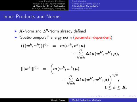
Inner Products and Norms
I X-Norm and L2-Norm already definedI “Spatio-temporal” energy norm (parameter-dependent)
(((wk, vk)))du = m(wk, vk;µ)
+K∑k′=k
∆t a(wk′, vk
′;µ),
|||wk|||du =(m(wk, wk;µ)
+K∑k′=k
∆t a(wk′, wk
′;µ)
)1/2
,
1 ≤ k ≤ K.
Grepl, Rozza Model Reduction Methods

Linear Parabolic ProblemsReduced Basis ApproximationA Posteriori Error EstimationPOD(t)-Greedy(µ) Sampling
PreliminariesPrimal-only FormualationPrimal-Dual FormulationNumerical Results
Dual Final Condition
If m or ` are parameter-dependent, we define the residual
rΨf (v;µ) ≡ `(v;µ)−m(v,ΨK+1N ;µ), ∀ v ∈ X.
Lemma (Dual Error Bound – Final Condition)
Given µ ∈ D, the error edu(tK+1;µ) = ΨK+1(µ)−ΨK+1N (µ)
is bounded by
‖edu(tK+1;µ)‖ ≤ ∆ΨfN (µ) ≡
εΨfN (µ)
σLB(µ)
where
εΨfN (µ) ≡ sup
v∈X
rΨf (v;µ)
‖v‖
Grepl, Rozza Model Reduction Methods

Linear Parabolic ProblemsReduced Basis ApproximationA Posteriori Error EstimationPOD(t)-Greedy(µ) Sampling
PreliminariesPrimal-only FormualationPrimal-Dual FormulationNumerical Results
Dual Norm of Dual Residual
We define the residual, ∀k ∈ K,
rdu,k(v;µ) ≡ −m(v, ΨN (tk;µ)−ΨN (tk+1;µ)
∆t;µ)
−a(v,ΨN(tk;µ);µ), ∀ v ∈ X
Dual Norm of Residual
Given µ ∈ D, the dual norm of rdu,k(v;µ) is defined as
‖rdu,k(·;µ)‖X′ ≡ supv∈X
rdu,k(v;µ)
‖v‖X= ‖edu,k(µ)‖X ,
where edu,k(µ) ∈ X satisfies(edu,k(µ), v)X = rdu,k(v;µ), ∀v ∈ X.
Grepl, Rozza Model Reduction Methods

Linear Parabolic ProblemsReduced Basis ApproximationA Posteriori Error EstimationPOD(t)-Greedy(µ) Sampling
PreliminariesPrimal-only FormualationPrimal-Dual FormulationNumerical Results
Energy Error Bound – Dual
We define the error bound, ∆du,kN (µ) = ∆du
N (tk;µ),1 ≤ k ≤ K, as
∆du,kN (µ) =
(∆t
αLB(µ)
k∑k′=1
‖edu,k′(µ)‖2X + σLB(µ)∆ΨfN (µ)2
)1/2
.
We can then prove
Proposition (Energy Error Bound)
For any N = 1, . . . , Ndu,max, the error in the dual variable,edu,k(µ) = Ψk(µ)−Ψk
N(µ), is bounded by
|||edu,k(µ)|||du ≤ ∆du,kN (µ), ∀ µ ∈ D, ∀ k ∈ K.
Grepl, Rozza Model Reduction Methods

Linear Parabolic ProblemsReduced Basis ApproximationA Posteriori Error EstimationPOD(t)-Greedy(µ) Sampling
PreliminariesPrimal-only FormualationPrimal-Dual FormulationNumerical Results
Output Error Bound
We (re-)define the output error bound, ∆s kN (µ) = ∆s
N(tk;µ),1 ≤ k ≤ K, as.
∆s kN (µ) ≡ ∆pr,k
Npr(µ) ∆du,K−k+1
Ndu(µ)
Proposition (Simple Output Error Bound)
For any N = 1, . . . , Nmax, the error in the output is bounded by
|sk(µ)− skN(µ)| ≤ ∆s kN (µ), ∀µ ∈ D, ∀k ∈ K.
Grepl, Rozza Model Reduction Methods

Linear Parabolic ProblemsReduced Basis ApproximationA Posteriori Error EstimationPOD(t)-Greedy(µ) Sampling
PreliminariesPrimal-only FormualationPrimal-Dual FormulationNumerical Results
Offline-Online Decomposition
Computational procedure to calculate ‖edu,k(µ)‖X , ∀k ∈ K,follows directly from the primal problem
I Expand ΨN(µ) =Ndu∑j=1
ΨkN j(µ) ζdu,j
I Riesz representation:(edu,k(µ), v)X = rdu,k(v;µ)
I Affine decomposition
I Linear superposition
Grepl, Rozza Model Reduction Methods

Linear Parabolic ProblemsReduced Basis ApproximationA Posteriori Error EstimationPOD(t)-Greedy(µ) Sampling
PreliminariesPrimal-only FormualationPrimal-Dual FormulationNumerical Results
Offline-Online Decomposition
Summary of computational cost: Q = Qa +Qm
OFFLINE —
O(Q(Npr,max +Ndu,max)N •) + O(Q2(N2pr,max +N2
du,max)N )solve Poisson problems form µ-independent inner products
;
ONLINE —
O(KQ2(N2pr +N2
du))evaluate ‖epr/du,k(µ)‖X -sum for 1 ≤ k ≤ K
;
Online cost is independent of N .
Grepl, Rozza Model Reduction Methods

Linear Parabolic ProblemsReduced Basis ApproximationA Posteriori Error EstimationPOD(t)-Greedy(µ) Sampling
PreliminariesPrimal-only FormualationPrimal-Dual FormulationNumerical Results
Summary
Remarks:
I We require a separate dual problem for each output⇒ Primal-dual formulation becomes expensive.
I Shifting property for dual only holds for LTI systems⇒ Bounds are valid also for linear time-varying systems,
but we require K dual problems (for each output).
I Computational cost: two smaller problems are “better” thanone big problem, e.g., consider Npr = Ndu = 1/2N .
I Residual correction term: O(K(K + 1)NprNdu)⇒ Reduce cost by considering only every (say) tenth timestep.
Grepl, Rozza Model Reduction Methods

Linear Parabolic ProblemsReduced Basis ApproximationA Posteriori Error EstimationPOD(t)-Greedy(µ) Sampling
PreliminariesPrimal-only FormualationPrimal-Dual FormulationNumerical Results
Example: Concrete Delamination – Results
Delamination
Heat Flux
FRP laminate
q(t)
x1
Concrete slab
x2
κ
ΓF
wdel
Ω2 , Measurement 2
Γdel
, Measurement 1Ω1
Ω0,FRP%FRP, cP,FRP, kFRP
Ω0,C%C, cP,C, kC 1 [kC]
y0(x, t = 0;µ) = 0
Input (parameter): µ ≡ (wdel/2, κ ≡ kFRP/kC) ⊂ D,where D ≡ [1, 10]× [0.4, 1.8].
“Truth”: N = 5601, K = 200.
Grepl, Rozza Model Reduction Methods

Linear Parabolic ProblemsReduced Basis ApproximationA Posteriori Error EstimationPOD(t)-Greedy(µ) Sampling
PreliminariesPrimal-only FormualationPrimal-Dual FormulationNumerical Results
Example: Concrete Delamination – Results
Dual problem: convergence energy norm error & bound output 1
Ndu εdumax,rel ∆du
max,rel ηdu
20 2.04E –01 7.46E –01 2.6240 5.23E –02 9.69E –02 2.4160 1.36E –02 2.23E –02 2.5680 3.30E –03 5.39E –03 2.61100 1.74E –03 2.27E –03 2.29120 6.45E –04 9.00E –04 2.25140 1.51E –04 3.77E –04 2.13160 8.16E –05 1.41E –04 2.09
Grepl, Rozza Model Reduction Methods

Linear Parabolic ProblemsReduced Basis ApproximationA Posteriori Error EstimationPOD(t)-Greedy(µ) Sampling
PreliminariesPrimal-only FormualationPrimal-Dual FormulationNumerical Results
Example: Concrete Delamination – Results
Primal-dual formulation: convergence output bound (Npr = Ndu)
N εsmax,rel ∆smax,rel ηs
20 1.78E –02 1.23E+00 17440 1.75E –03 3.85E –02 26060 1.67E –04 2.24E –03 18980 7.57E –06 2.43E –04 268100 6.21E –07 3.21E –05 222120 1.34E –07 6.84E –06 212140 3.36E –08 1.82E –06 210160 8.64E –09 4.14E –07 384
εs,simplemax,rel ∆s,simple
max,rel
6.76E –02 2.58E+011.44E –02 6.24E+003.34E –03 1.46E+001.43E –03 4.73E –013.71E –04 2.77E –019.81E –05 1.24E –014.59E –05 6.33E –022.34E –05 2.88E –02
Grepl, Rozza Model Reduction Methods

Linear Parabolic ProblemsReduced Basis ApproximationA Posteriori Error EstimationPOD(t)-Greedy(µ) Sampling
PreliminariesPrimal-only FormualationPrimal-Dual FormulationNumerical Results
Example: Concrete Delamination – Results
Primal-dual formulation: convergence output error and bound
20 40 60 80 100 120 140 160 180 20010
−9
10−8
10−7
10−6
10−5
10−4
10−3
10−2
10−1
Npr
ε max
,rel
s
Ndu
= 20N
du = 40
Ndu
= 80N
du = 120
Ndu
= 140N
du = 160
20 40 60 80 100 120 140 160 180 20010
−7
10−6
10−5
10−4
10−3
10−2
10−1
100
101
Npr
∆ max
,rel
s
Ndu
= 20N
du = 40
Ndu
= 80N
du = 120
Ndu
= 140N
du = 160
Grepl, Rozza Model Reduction Methods

Linear Parabolic ProblemsReduced Basis ApproximationA Posteriori Error EstimationPOD(t)-Greedy(µ) Sampling
PreliminariesPrimal-only FormualationPrimal-Dual FormulationNumerical Results
Example: Concrete Delamination – Results
Primal-dual formulation: online compuational times
Npr = Ndu sN(µ, tk) ∆sN(µ, tk) s(µ, tk)
20 3.11E –03 9.78E –04 140 5.22E –03 1.54E –03 160 7.90E –03 2.34E –03 180 9.49E –03 3.88E –03 1100 1.48E –02 9.98E –03 1120 2.01E –02 1.74E –02 1140 2.55E –02 3.21E –02 1160 3.10E –02 4.36E –02 1
Output & Bound for 1 ≤ k ≤ KSavings with respect to truth: ≈ 150
Grepl, Rozza Model Reduction Methods

Linear Parabolic ProblemsReduced Basis ApproximationA Posteriori Error EstimationPOD(t)-Greedy(µ) Sampling
PreliminariesPrimal-only FormualationPrimal-Dual FormulationNumerical Results
Example: Concrete Delamination – Results
Primal-dual formulation: online compuational times
Npr = Ndu sN(µ, tk) ∆sN(µ, tk) s(µ, tk)
20 6.90E –04 9.78E –04 140 9.70E –04 1.54E –03 160 1.31E –03 2.34E –03 180 1.82E –03 3.88E –03 1100 2.97E –03 9.98E –03 1120 5.59E –03 1.74E –02 1140 9.28E –03 3.21E –02 1160 1.23E –02 4.36E –02 1
Output & Bound for every tenth timestep k = [10, 20, . . . ,K]
Savings with respect to truth: ≈ 400
Grepl, Rozza Model Reduction Methods

Linear Parabolic ProblemsReduced Basis ApproximationA Posteriori Error EstimationPOD(t)-Greedy(µ) Sampling
PreliminariesPrimal-only FormualationPrimal-Dual FormulationNumerical Results
Example: Concrete Delamination – Results
Primal formulation: online compuational times
Npr sN(µ, tk) ∆sN(µ, tk) s(µ, tk)
20 2.10E –04 4.52E –04 140 3.97E –04 6.36E –04 160 6.73E –04 8.75E –04 180 1.08E –03 1.33E –03 1100 2.05E –03 3.70E –03 1120 4.37E –03 6.20E –03 1140 6.44E –03 1.20E –02 1160 8.24E –03 1.65E –02 1
Output & Bound for every timestep 1 ≤ k ≤ KSavings with respect to truth: ≈ 40
Grepl, Rozza Model Reduction Methods

Linear Parabolic ProblemsReduced Basis ApproximationA Posteriori Error EstimationPOD(t)-Greedy(µ) Sampling
PreliminariesPrimal-only FormualationPrimal-Dual FormulationNumerical Results
Summary
I Choice primal-dual vs. primal-only formulation is problemspecific and depends on
I convergence rate of primal problem.I convergence rate of dual problem.I number of outputs.
I Same argument holds for choice of Npr vs. Ndu.I Primal-only formulation advantageous if
I K is large, i.e., K N ; complexity for residual correction isO(K(K + 1)NprNdu).
I we have many outputs are of interest (separate dual for eachoutput).
I the system is time-varying.
Grepl, Rozza Model Reduction Methods

Linear Parabolic ProblemsReduced Basis ApproximationA Posteriori Error EstimationPOD(t)-Greedy(µ) Sampling
MotivationPOD in timeGreedy in parameter spaceSummary
Sampling Strategy
We extend the Greedy Algorithm to a POD(t)-Greedy(µ) samplingprocedure [HO], combining a
I small POD in time, with⇒ optimally captures causality of time variation
I (exhaustive) Greedy search in parameter space D.⇒ (sub-)optimal selection for high-dimensional D (large ntrain).
We defineI Desired error tolerance εtol,min.I Train sample Ξtrain ≡ µ1
train, . . . , µntraintrain ⊂ D, with
I Cardinality (size) |Ξtrain| = ntrain.⇒ Ξtrain serves as our (finite) surrogate for D.
Grepl, Rozza Model Reduction Methods

Linear Parabolic ProblemsReduced Basis ApproximationA Posteriori Error EstimationPOD(t)-Greedy(µ) Sampling
MotivationPOD in timeGreedy in parameter spaceSummary
POD(t)-Greedy(µ)
Proper Orthogonal Decomposition (POD) in time:
I LetPODX(uk(µ), 1 ≤ k ≤ K, R)
return the R largest POD modes, ΨPOD,i, 1 ≤ i ≤ R,with respect to the (·, ·)X inner product.
I The set PR = ΨPOD,i, 1 ≤ i ≤ R is (·, ·)X orthogonaland satisfies the optimality property
PR = arg infXR⊂spanuk(µ),1≤k≤K
(1K
K∑k=1
infv∈XR
‖uk(µ)− v‖2X
)1/2
Grepl, Rozza Model Reduction Methods

Linear Parabolic ProblemsReduced Basis ApproximationA Posteriori Error EstimationPOD(t)-Greedy(µ) Sampling
MotivationPOD in timeGreedy in parameter spaceSummary
POD(t)-Greedy(µ)
Evaluation of ΨPOD,1 = PODX(uk(µ), 1 ≤ k ≤ K, 1):
1. Form correlation matrix CPOD ∈ RK×K given by
CPODij = 1
K(ui(µ), uj(µ))X , 1 ≤ i, j ≤ K.
2. Solve for eigenpair (ψPOD,max ∈ RK , λPOD,max ∈ R+0),corresponding to largest eigenvalue λPOD,max from
CPOD ψPOD,k = λPOD,kψPOD,k.
3. Compute largest POD mode
ΨPOD,1 ≡K∑k=1
ψPOD,maxk uk(µ).
Grepl, Rozza Model Reduction Methods

Linear Parabolic ProblemsReduced Basis ApproximationA Posteriori Error EstimationPOD(t)-Greedy(µ) Sampling
MotivationPOD in timeGreedy in parameter spaceSummary
POD(t)-Greedy(µ)
We require a rigorous, sharp, inexpensive error bound:
|||uk(µ)− ukN(µ)||| ≤ ∆kN(µ), ∀µ ∈ D.
RecallI Effectivities ηu are O(1).I Computational cost to evaluate ∆k
N(µ) is O(KQ2N2).
Greedy(µ) Idea:I ∆k
N(µ) is monotonically increasing in time.I Find parameter value such that
µ∗ = arg maxµ∈Ξtrain
∆KN(µ)
⇒ Largest error bound at final time.
Grepl, Rozza Model Reduction Methods

Linear Parabolic ProblemsReduced Basis ApproximationA Posteriori Error EstimationPOD(t)-Greedy(µ) Sampling
MotivationPOD in timeGreedy in parameter spaceSummary
POD(t)-Greedy(µ)
Greedy, L∞(Ξtrain, ||| · |||), space “economization”
Kntrain contestants
∈ Ξtrain × I
⇒ Nmax Kntrain winners
µ∗1, . . . , µ∗Nmax
in which we never form most snapshots:
|||uk(µ)− ukN(µ)|||ntrain · O(KN •)
replaced
by
∆kN(µ)
ntrain · O(KQ2N2) †
note good effectivity of estimator is crucial.
†In addition to the offline effort that is requiredin any event for online rigorous/sharp certification.
Grepl, Rozza Model Reduction Methods

Linear Parabolic ProblemsReduced Basis ApproximationA Posteriori Error EstimationPOD(t)-Greedy(µ) Sampling
MotivationPOD in timeGreedy in parameter spaceSummary
POD(t)-Greedy(µ) Algorithm
POD(t)-Greedy(µ) Algorithm
Set XN = 0, SN = 0, N = 0, µ∗ = µ∗0
while ∆maxN ≥ εtol,min
ekN,proj(µ∗) = uk(µ∗)− projX,XNu
k(µ∗), 1 ≤ k ≤ KSN+1 = SN ∪ µ∗;XN+1 = XN + PODX(ekN,proj(µ
∗), 1 ≤ k ≤ K, 1);
N = N + 1;
µ∗ = arg maxµ∈Ξtrain
∆KN(µ)/|||yKN (µ)|||;
∆maxN = ∆K
N(µ∗)/|||yKN (µ∗)|||;end
Grepl, Rozza Model Reduction Methods

Linear Parabolic ProblemsReduced Basis ApproximationA Posteriori Error EstimationPOD(t)-Greedy(µ) Sampling
MotivationPOD in timeGreedy in parameter spaceSummary
POD(t)-Greedy(µ)
RemarksI Spaces XN are hierarchical.
I Algorithm guarantees that
|||uk(µ)− ukN(µ)||| ≤ ∆kN(µ) ≤ εtol,min, ∀µ ∈ Ξtrain.
I We can replace condition on ∆maxN by a condition on Nmax
(hp-Reduced Basis).
I No additional Gram-Schmidt orthogonalization required, basisfunctions are "by construction" X-orthogonal.
I Computational complexity remains O(KN •) + O(ntrain) –not O(KN •ntrain).
Grepl, Rozza Model Reduction Methods

Linear Parabolic ProblemsReduced Basis ApproximationA Posteriori Error EstimationPOD(t)-Greedy(µ) Sampling
MotivationPOD in timeGreedy in parameter spaceSummary
Extensions
I Nonzero initial conditions, u0(µ) 6= 0.I Nonzero (but constant) initial condition
⇒ ζ1 = u0(µ) 6= 0.I Affinely parameter dependent initial condition
u0(µ) =Qu0∑q=1
Θqu0
(µ)uq0
where uq0 ∈ X, µ-independent and known, andΘqu0
: D → R, µ-dependent functions.We then initialize
⇒ XN = spanuq0, 1 ≤ q ≤ Qu0.I No a priori knowledge
– Series representation of u0;– Projection of u0 onto XN (N -dependent cost);– Contribution to error & bound.
Grepl, Rozza Model Reduction Methods

Linear Parabolic ProblemsReduced Basis ApproximationA Posteriori Error EstimationPOD(t)-Greedy(µ) Sampling
MotivationPOD in timeGreedy in parameter spaceSummary
Extensions
I Unknown “control” input, g(tk) (e.g. optimal control).Duhamel’s Principle: given any control input g(tk), we canobtain uk(µ) from
uk(µ) =K∑j=1
h(tk−j+1;µ) g(tj), ∀k ∈ K,
where h(tk;µ) is the impulse response. We thus train the RBapproximation on an impulse input
⇒ g(tk) = δ1k, ∀k ∈ K.only valid for LTI systems
I Multiple “control” inputs, g(tk) ∈ Rm.⇒ recursive training on each input (LTI).
Grepl, Rozza Model Reduction Methods

Linear Parabolic ProblemsReduced Basis ApproximationA Posteriori Error EstimationPOD(t)-Greedy(µ) Sampling
Extensions & Outlook
Straightforward:I Non-symmetric Problems (convection-diffusion)
I Define norms appropriately (replace a by symmetric part of a)I Adjust time discretization (Crank-Nicolson instead of EB)I Expect much larger N (need for hpRB)
I Dynamic systems (parametric or non-parametric).
Not Straightforward:I Non-affine Problems
I Empirical Interpolation MethodI Non-parabolic (hyperbolic) Problems
I a non-coercive: L2(Ω) error bound.I Expect even larger N .
Grepl, Rozza Model Reduction Methods

Linear Parabolic ProblemsReduced Basis ApproximationA Posteriori Error EstimationPOD(t)-Greedy(µ) Sampling
Extensions & Outlook
Not Straightforward:I Non-linear Problems
I Quadratically Nonlinear (visc. Burgers [NRP], Navier Stokes[VP, KNP])
I Lower bounds for stability constantI Online cost for ∆N is O(N4)I Bounds restricted to envelope tf ×Re small
I Higher-Order & Nonpolynomial NonlinearI Empirical Interpolation Method
I Multiscale ProblemsI Fokker-Plank Equation
Grepl, Rozza Model Reduction Methods