modeling of an interface crack with bridging effects...
TRANSCRIPT
Modeling of an Interface
Crack with Bridging Effects
Between Two Fibrous
Composite Layers
Brian Lau Verndal Bak
Thomas Bro Henriksen
Department of Mechanical and
Manufacturing Engineering
Aalborg University
Spring 2010
Master of Science Thesis
Design of Mechanical Systems

Study Board of Industry and
Global Business Development
Design of Mechanical Systems
Fibigerstræde 16
Telephone: 99 40 93 09
Email: [email protected]
http://industri.aau.dk/
Title: Modeling of an Interface Crack with Bridging Effects
Between Two Fibrous Composite Layers
Theme: Design of Mechanical Systems
Project Period: DMS4, Spring 2010
Project Group: Group 48F
Supervisor:
Jens H. Andreasen
Authors:
Brian Lau Verndal Bak Thomas Bro Henriksen
Copies: 4
Report: 118 pages
DVD: 1
Finished: June 2nd 2010
The content of this report is freely accessible, though publication (with reference) may only
occur after permission from the authors.

Abstract
In this report a procedure for analyzing the fracture resistance of interface cracks between sim-
ilar or dissimilar layers of fibrous composite materials is developed. This is intended for a de-
tailed simulation of delamination defects using fracture mechanics, as they cannot be analyzed
by use of point stress or strain based criteria.
In advanced composite structures a significant amount of resources are spent on inspec-
tion and repair of production errors like dry-spots, which are areas where fibers have not been
wetted by the resin. The developed procedure is intended to be used to evaluate whether or
not a dry-spot or another kind of detected delamination in a composite structure is critical for
the structural integrity, and therefore has to be repaired.
The propagation of cracks in fibrous materials is considered to be dependent on the critical
energy release rate Gc ,0 at the crack tip, as well as the crack length and end-opening due to
fiber bridging across the crack faces behind the crack tip. Fiber bridging increases the fracture
resistance against crack propagation until reaching a steady state crack length for which it is
assumed constant, and this is accounted for in the developed procedure.
The criteria for determining propagation implies that the energy release rate at the crack
tip must reach a material dependent critical value G0 ≥ Gc ,0. The energy release rate G0 is
calculated from the stress intensity factors, and these are estimated by use of the analytical
expression for crack face displacements near the crack tip. The increase in fracture resistance
from fiber bridging influences this criterion by causing tractions between the crack faces and
thereby reduce the relative crack displacement. This means that an increased load can be ap-
plied before the critical values are reached.
An extensive study of fracture mechanical theory concerning interface cracks between two
isotropic or anisotropic materials, with focus on obtaining expressions for the relative displace-
ment of the crack faces, has been conducted and is described in this report.
A numerical method for simulating this criterion for a specific delamination crack based
on solving the structural response using a finite element model is described. Results for the
relative crack face displacement near the crack tip are exported to a parameter estimation used
for determining the stress intensity factors related to the analytical expressions. This parameter
estimation is formulated as an optimization problem minimizing the least squares difference
between the numerical results and the analytical expressions by use of the conjugate gradient
method with a golden section search.
In fracture mechanics the expressions for the relative crack face displacement are derived
as infinite series of eigenfunctions, but in most literature they are presented by the first eigen-
function which only applies very close to the crack tip. As this calls for using small elements
compared to structural dimensions in order to yield reliable results in the numerical procedure,
analytical expressions for the relative displacement including the second and third eigenfunc-
tions are derived.
These are implemented in the parameter estimation, and studies of the determination of the
stress intensity factors show that it yields reliable estimation results for elements up to 10-20
times larger than when using the expressions with the first eigenfunction only. Similar studies
have been conducted for orthotropic materials with the same conclusion.
v

vi
A simulation of propagation of a crack in two similar orthotropic fiber materials with bridg-
ing is conducted for a plane DCB model in order to verify the modeling of fiber bridging based
on assumed test results. The resulting R-curves are compared to these and show good corre-
lation for the pure mode I and mode II, while for a mixed mode case the steady state fracture
resistance is overestimated.

Preface
This Master of Science Thesis is the product of the DMS4 project period of Spring 2010 at Aal-
borg University, Department of Mechanical and Manufacturing Engineering. It has been pub-
lished by group 48F. The purpose of this project is to simulate an interface crack with bridging
effects between two fibrous composite layers.
The report is most of all directed to the supervisor and censor but also fellow students with
an interest in this subject. The reader is assumed familiar with linear fracture mechanics of
isotropic materials as well as fibrous composite materials in order to understand the contents
of this report.
Structure of the Report
This report consists of a main report accompanied by an appendix in the back of the report. A
detailed description of the approach to the project and the structure of the report is given in
chapter 1. The appendix part consists of supplementary information and calculations to the
parts of the report. There are references from the report to the appendix where appropriate.
Computational calculations are made in MATLAB, analytical expressions are derived using
Maple and all finite element analysis are made in ANSYS. All programs and macros used to
build and analyze the models studied in this project can be found on the appertaining DVD.
Instructions for Reading
It is expected that the chapters are read together and in their chronological order. The notation
used for references in the report is as is in agreement with the Harvard citation style. The used
sources are listed in the bibliography in the back of the main report. Figures and tables are
numbered sequentially in each chapter and references are made to all figures and tables. The
report contains a nomenclature located at on page ix.
Contents of the appertaining DVD
The contents of the enclosed DVD are:
• PDF files of this report
• All MATLAB and Maple programs used in the project
• All macros for generating the finite element models
vii

Nomenclature
(δy )i Relative displacement between nodepair i
α, β Dundurs’ parameters
δ Crack mouth opening displacement, CMOD
δn , δt Relative normal and tangential displacement of crack faces
δx , δy , δz Relative displacement in x-, y- and z-direction
Γ J-integral path
κ Poisson parameter for plane stress or strain
λ Singularity parameter
d(x) Relative displacement vector
f(z) Complex potential vector
h(x) Vector relating the complex potential vectors for material 1 and 2
t(x) Traction vector
w3 Eigenvector
w Eigenvector
µ Shear module
µ Complex root of sixth order characteristic equation
ν Poission’s ratio
Φ(z) Complex stress potential defined as ddz
φ(z)
φ(z) Complex stress potential
Ψ(z) Complex stress potential defined as ddz
ψ(z)
ψ(z) Complex stress potential
σnn ,σt t Stress components rotated according to the nt-coordinate system
σn ,σt Normal and tangential stresses on crack faces from fiber bridging
θ Argument for complex number
θ Rotation angle
ε Bimaterial constant
A Matrix describing the mechanical properties of an anisotropic material
A j ,B j ,C j ,D j Complex material parameters
B Matrix describing the mechanical properties of an anisotropic material
B Width of the DCB test specimen
C Constant dependent on material and geometry
ix

x
E Youngs Modulus for an isotropic material
G Energy release rate
Gc Critical energy release rate
H Height of each beam of the DCB test specimen
H Matrix describing the mechanical properties of an anisotropic bimaterial combination
I Second area moment
j Index for material 1 or material 2
JR Critical fracture resistance
K Complex stress intensity factor (K I + i K I I )
k Index for eigenvalue: 0 = main eigenvalue, 1 = second eigenvalue,...
K I Stress intensity factor for mode I
K I I I Stress intensity factor for mode III
K I I Stress intensity factor for mode II
L Length
L Matrix describing the mechanical properties of an anisotropic material
M1 Moment on the upper beam
M2 Moment on the lower beam
q1, q2 Weighting factors
ri Distance from the crack tip to nodepair i
Si j Compliance matrix
t Thickness
u, v , w Displacement in x-, y- and z-direction
Zi Parameters used in the parameter estimation procedure
r Distance from crack tip

xi
.

Contents
Abstract vii
Preface viii
Nomenclature x
1 Project Description 1
1.1 Project Introduction . . . . . . . . . . . . . . . . . . . . . . . . . . . . . . . . . . . . 1
1.2 Problem Statement . . . . . . . . . . . . . . . . . . . . . . . . . . . . . . . . . . . . 5
1.3 Project Approach . . . . . . . . . . . . . . . . . . . . . . . . . . . . . . . . . . . . . 5
1.4 Project limitations . . . . . . . . . . . . . . . . . . . . . . . . . . . . . . . . . . . . . 7
1.5 Structure of the report . . . . . . . . . . . . . . . . . . . . . . . . . . . . . . . . . . 7
2 Crack in a Single Isotropic Material 9
2.1 Stresses and Displacements Around a Crack Tip . . . . . . . . . . . . . . . . . . . 9
2.2 Simulation of a Crack in a Isotropic Material. . . . . . . . . . . . . . . . . . . . . . 12
3 Interface Crack between Two Isotropic Materials 21
3.1 Theory of Interfacial Crack Between Two Isotropic Materials . . . . . . . . . . . . 22
3.2 Simulation of a Crack Between Two Dissimilar Isotropic Materials . . . . . . . . 33
3.3 Presentation of Simulation Results . . . . . . . . . . . . . . . . . . . . . . . . . . . 40
3.4 Evaluation of the Results of the Parameter Estimation . . . . . . . . . . . . . . . . 43
4 Interface Crack between Two Dissimilar Anisotropic Materials 45
4.1 Theory of Interface Crack between Dissimilar Anisotropic Materials . . . . . . . 45
4.2 Fiber Bridging . . . . . . . . . . . . . . . . . . . . . . . . . . . . . . . . . . . . . . . 53
4.3 Finite Element Modeling of Bridging . . . . . . . . . . . . . . . . . . . . . . . . . . 57
4.4 Description of Test Data . . . . . . . . . . . . . . . . . . . . . . . . . . . . . . . . . 60
4.5 Simulation of Crack between Two Orthotropic Materials . . . . . . . . . . . . . . 62
4.6 Analysis of DCB Test Specimen with a Solid FE Model . . . . . . . . . . . . . . . . 69
5 Discussion 77
5.1 Application of the Developed Procedure . . . . . . . . . . . . . . . . . . . . . . . . 77
5.2 Further Development . . . . . . . . . . . . . . . . . . . . . . . . . . . . . . . . . . . 80
Conclusion 88
Bibliography 89
APPENDIX 93
Appendix A Simulation Results for Isotropic Bimaterial Problem 93
A.1 Results Based on Complete 2 Termed Displacement Expansion . . . . . . . . . . 93
A.2 Results Based on Simplified 2 Termed Displacement Expansion . . . . . . . . . . 94
xiii

xiv CONTENTS
A.3 Results Based on Complete 3 Termed Displacement Expansion . . . . . . . . . . 98
A.4 Results Based on Simplified 3 Termed Displacement Expansion . . . . . . . . . . 100
Appendix B Simulation Results for Anisotropic Bimaterial Problem 103

Chapter
1Project Description
In this chapter the subject of the project is presented and the motivation for treating it is ex-
plained. Furthermore, the problem statement and the limitations to the project are clarified and
a description of the approach adopted for conducting the project is given in order to give an
overview of the contents of the project.
1.1 Project Introduction
In this report the development of a numerical procedure based on fracture mechanics to be
used for evaluating stability of a crack in the interface between two fiber composite materials
is described. A significant number of mechanical structures such as wind turbine blades, boats
and aircrafts are designed with use of fiber composite materials in order to reduce weight, and
this gives rise to a wish for improved methods for predicting design limits for these structures.
At present, fiber composite structures are almost exclusively designed and analyzed on basis of
layered shell element models with design limits being determined from in-plane stress or strain
criteria. These criteria do not take out-of-plane effects into consideration which are one of the
major causes to fiber layer delamination and related failure of the structure. It is the intension
to be able to model this for details in the form of sub-models of a larger model/structure with
the procedure developed in this project.
The intended use of the numerical procedure developed in this project is to be able to pre-
dict whether a delamination crack in a structure caused by for example a production flaw is
critical to the integrity of the structure or not. In this way it can be assessed if the crack should
be repaired or not. The goal is to be able to determine a stability criteria for a crack and the
effect on this criteria caused by fibers across the two crack surfaces behind the crack tip, the
so-called bridging effect.
Research in the field of modeling of crack propagation in composite structures is extensive
and ongoing. In the wind turbine and aviation industry the long termed goals are to be able to
model and analyze crack propagation in large structures such as wind turbine blades or aircraft
wings, and in a lager perspective to be able to assess and predict the consequences of fatigue
crack growth in composite structures.
The main alternative to the method used in the procedure treated in this project is cohesive
modeling which uses elements formulated with a cohesive constitutive law that implies both
1
2 CHAPTER 1. PROJECT DESCRIPTION
crack tip growth and bridging effects. Cohesive modeling has been a significant area of research
at Aalborg University in recent years, see for instance (Hansen, 2009).
1.1.1 Concept of Crack Instability Criteria and Bridging
The concept of crack instability criteria with bridging is introduced here in order to clarify the
purpose of the method used in the numerical procedure developed. A crack in any given struc-
ture of common materials have a fracture toughness against crack growth. The fracture tough-
ness, which is material dependent, is quantified by the critical energy release rate Gc
[
Jm2
]
.
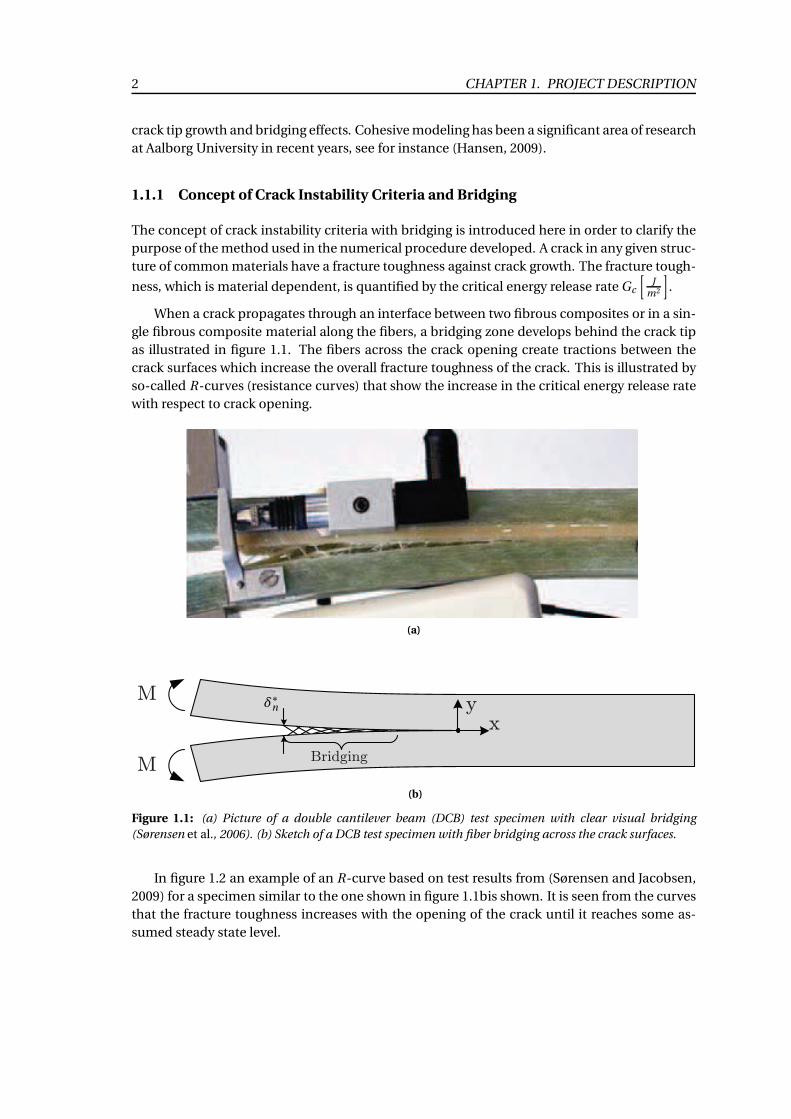
When a crack propagates through an interface between two fibrous composites or in a sin-
gle fibrous composite material along the fibers, a bridging zone develops behind the crack tip
as illustrated in figure 1.1. The fibers across the crack opening create tractions between the
crack surfaces which increase the overall fracture toughness of the crack. This is illustrated by
so-called R-curves (resistance curves) that show the increase in the critical energy release rate
with respect to crack opening.
(a)
M
M
xy
Bridging
δ∗n
(b)
Figure 1.1: (a) Picture of a double cantilever beam (DCB) test specimen with clear visual bridging
(Sørensen et al., 2006). (b) Sketch of a DCB test specimen with fiber bridging across the crack surfaces.
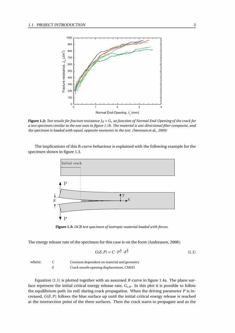
In figure 1.2 an example of an R-curve based on test results from (Sørensen and Jacobsen,
2009) for a specimen similar to the one shown in figure 1.1bis shown. It is seen from the curves
that the fracture toughness increases with the opening of the crack until it reaches some as-
sumed steady state level.
1.1. PROJECT INTRODUCTION 3
Figure 1.2: Test results for fracture resistance JR =Gc as function of Normal End-Opening of the crack for
a test specimen similar to the one seen in figure 1.1b. The material is uni-directional fiber composite, and
the specimen is loaded with equal, opposite moments in the test. (Sørensen et al., 2009)
The implications of this R-curve behaviour is explained with the following example for the
specimen shown in figure 1.3.
xy
P
P
Initial crack
δ
Figure 1.3: DCB test specimen of isotropic material loaded with forces.
The energy release rate of the specimen for this case is on the form (Andreasen, 2008):
G(δ,P) =C ·P43 ·δ
23 (1.1)
where: C Constant dependent on material and geometry
δ Crack mouth opening displacement, CMOD
Equation (1.1) is plotted together with an assumed R-curve in figure 1.4a. The plane sur-
face represent the initial critical energy release rate, Gc ,0. In this plot it is possible to follow
the equilibrium path (in red) during crack propagation. When the driving parameter P is in-
creased, G(δ,P) follows the blue surface up until the initial critical energy release is reached
at the intersection point of the three surfaces. Then the crack starts to propagate and as the
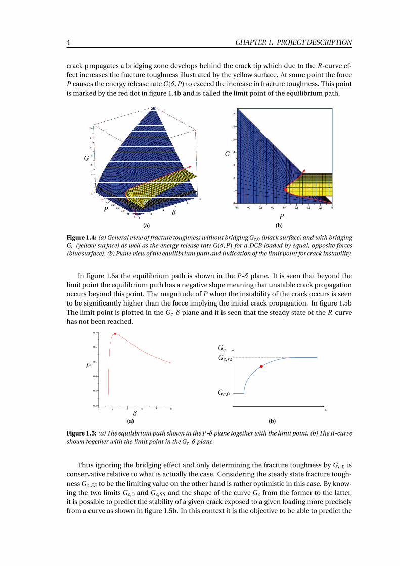
4 CHAPTER 1. PROJECT DESCRIPTION
crack propagates a bridging zone develops behind the crack tip which due to the R-curve ef-
fect increases the fracture toughness illustrated by the yellow surface. At some point the force
P causes the energy release rate G(δ,P) to exceed the increase in fracture toughness. This point
is marked by the red dot in figure 1.4b and is called the limit point of the equilibrium path.
δP
G
(a)
P
G
(b)
Figure 1.4: (a) General view of fracture toughness without bridging Gc ,0 (black surface) and with bridging
Gc (yellow surface) as well as the energy release rate G(δ,P ) for a DCB loaded by equal, opposite forces
(blue surface). (b) Plane view of the equilibrium path and indication of the limit point for crack instability.
In figure 1.5a the equilibrium path is shown in the P-δ plane. It is seen that beyond the
limit point the equilibrium path has a negative slope meaning that unstable crack propagation
occurs beyond this point. The magnitude of P when the instability of the crack occurs is seen
to be significantly higher than the force implying the initial crack propagation. In figure 1.5b
The limit point is plotted in the Gc -δ plane and it is seen that the steady state of the R-curve
has not been reached.
δ
P
(a)
Gc
Gc ,0
Gc ,ss
(b)
Figure 1.5: (a) The equilibrium path shown in the P-δ plane together with the limit point. (b) The R-curve
shown together with the limit point in the Gc -δ plane.
Thus ignoring the bridging effect and only determining the fracture toughness by Gc ,0 is
conservative relative to what is actually the case. Considering the steady state fracture tough-
ness Gc ,SS to be the limiting value on the other hand is rather optimistic in this case. By know-
ing the two limits Gc ,0 and Gc ,SS and the shape of the curve Gc from the former to the latter,
it is possible to predict the stability of a given crack exposed to a given loading more precisely
from a curve as shown in figure 1.5b. In this context it is the objective to be able to predict the
1.2. PROBLEM STATEMENT 5
course of the fracture toughness curve from Gc ,0 to Gc ,ss for a specific crack by the procedure
developed in this project.
1.2 Problem Statement
The objective of this project is to develop a procedure for determining if a crack in an interface
between two dissimilar materials is critical to the integrity of a particular structure. Further-
more, the objective is to gain understanding of theory of advanced fracture mechanics describ-
ing interface cracks and how this can be implemented in numerical modeling procedures.
In order to do this, theory describing the physical behavior and growth of a crack in inter-
faces must be studied. This concern among other things analytical descriptions of the stresses
and crack face displacements near the crack tip including treatment of the coupled oscillating
stress singularity, determination of the stress intensity factors and the effects of crack mode
mixity. Furthermore, the increase in the fracture resistance, R-curve effects, caused by bridging
fibers behind the crack tip is treated. A numerical procedure for application of the full formu-
lation fracture mechanics near the crack tip, with a simulation of bridging effects in the crack
opening between the crack surfaces, has to be developed.
Finally, an application of the procedure on a two dimensional case for orthotropic fiber
composites has to be carried out in order to evaluate the simulation of the R-curve effects by
comparing it to R-curves inspired from tests conducted in (Sørensen and Jacobsen, 2009).
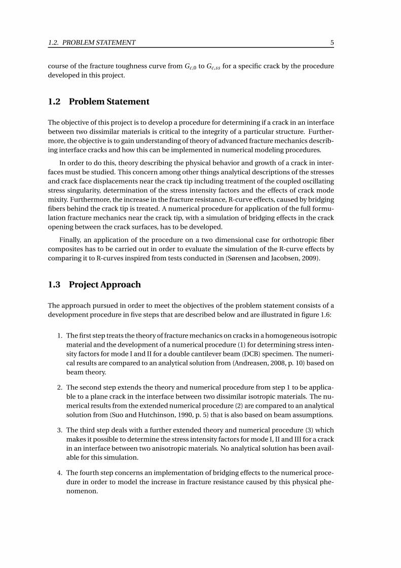
1.3 Project Approach
The approach pursued in order to meet the objectives of the problem statement consists of a
development procedure in five steps that are described below and are illustrated in figure 1.6:
1. The first step treats the theory of fracture mechanics on cracks in a homogeneous isotropic
material and the development of a numerical procedure (1) for determining stress inten-
sity factors for mode I and II for a double cantilever beam (DCB) specimen. The numeri-
cal results are compared to an analytical solution from (Andreasen, 2008, p. 10) based on
beam theory.
2. The second step extends the theory and numerical procedure from step 1 to be applica-
ble to a plane crack in the interface between two dissimilar isotropic materials. The nu-
merical results from the extended numerical procedure (2) are compared to an analytical
solution from (Suo and Hutchinson, 1990, p. 5) that is also based on beam assumptions.
3. The third step deals with a further extended theory and numerical procedure (3) which
makes it possible to determine the stress intensity factors for mode I, II and III for a crack
in an interface between two anisotropic materials. No analytical solution has been avail-
able for this simulation.
4. The fourth step concerns an implementation of bridging effects to the numerical proce-
dure in order to model the increase in fracture resistance caused by this physical phe-
nomenon.
6 CHAPTER 1. PROJECT DESCRIPTION
5. In the fifth and final step the simulation of R-curve behavior by the numerical procedure
developed is evaluated for pure mode I, pure mode II and a mixed mode example. The re-
sults are compared to R-curves inspired from tests conducted in (Sørensen and Jacobsen,
2009).
Simulation of a crack in a single isotropic material
Simulation of an interface crack
between 2 dissimilar isotropic materials
Simulation of an interface crack between
2 unidirectional ortotropic fibre materials
Analytical solution to the model of (1) for comparison and
verification of the model
Analytical solution to the model of (2) for comparison and verification of the
simulation
Analytical solutions
Material A
Material BMaterial A
Material A
Material B
Simulation of bridging effects by implementation of this to the simulation in (3) for fiber materials
Simulation and evaluation of R-curve effects and comparison with R-curves inspired
from tests for two identical orthotropic fiber materials with bridging
Material A
Material B
Figure 1.6: Flowchart illustrating the project approach. The analytical solutions for (1) and (2) are from
(Andreasen, 2008, p. 10) and (Suo and Hutchinson, 1990, p. 5), respectively
1.4. PROJECT LIMITATIONS 7
The structure of the project approach is based on a wish to treat the theory and numerical
simulation simultaneously and a stepwise verification of the developed procedure with rela-
tively simple examples.
1.4 Project limitations
The development of a procedure for determining stability of an interface crack in this report is
treated within the following limitations:
• The theory applied in the developed procedure is based on the assumptions of linear
fracture mechanics.
• The main focus is limited to straight crack growth in plane problems.
• The procedure is limited to existing cracks only, and it does not treat simulation of crack
initiation.
• The procedure is limited to simulating crack growth in a straight plane between two ma-
terials only. Thus changes of crack planes are not treated.
1.5 Structure of the report
This report is structured in the following four parts:
Introduction to the project In this part the general problem of interface crack growth is de-
scribed with an introduction to significant fracture mechanical concepts related to it.
The motivation for working with this type of crack problem and the aim of the project is
covered as well as a contextual connection to application areas is described.
Theory and simulations of a crack in isotropic materials This part covers two chapters that
describe the fracture mechanical theory used and the numerical procedures developed
for determining the stress intensity factors for a crack in a single and in the interface
between two dissimilar isotropic materials. Each chapter contains a description of the
theory followed by the application in the numerical procedure for each of the two cases.
Theory and simulation for crack in anisotropic materials This part contains a chapter con-
taining a description of theory of an analytical description of crack face displacements
for anisotropic materials, which is implemented in the simulation.
Furthermore the concept of fiber bridging is treated and a simulation method is de-
scribed and implemented in the simulation procedure.
The test and results from (Sørensen and Jacobsen, 2009) is described, and assumptions
made in this article are discussed based on a simulation of a three dimensional model of
the test specimen.
Finally a two dimensional simulation of a double cantilever specimen of orthotropic
fiber materials is described in order to evaluate the R-curve effects in comparison with
R-curves inspired from the article.
Discussion of the procedure developed This covers a general discussion and evaluation of the
simulation procedure developed, and puts it in into perspective with suggestions for
prospective developments and possible applications of the procedure.

Chapter
2Crack in a Single Isotropic Material
The purpose of this chapter is to briefly describe the stresses and displacement expressions for a
crack in an isotropic material. This makes the base for a description of a numerical determina-
tion of stress intensity factors for this type of crack by fitting finite element result for crack face
displacements to analytical expressions.
2.1 Stresses and Displacements Around a Crack Tip
In this section the expressions for stresses and displacements around the crack tip from the
linear elastic fracture mechanics (LEFM) for a crack in a single isotropic material are briefly
described and plotted.
The objective of this report is to develop a numerical method for determining stability of
a crack between two similar or dissimilar materials. In order to do this the energy release rate
for the crack has to be calculated for a specific load, and then compared to a critical value
that is material dependent. It is intended to do this by calculating the stress intensity factor(s)
based on finite element results of stresses or displacements. From the stress intensity factors
the energy release rate can be calculated.
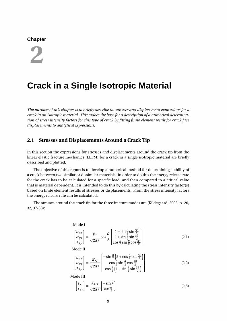
The stresses around the crack tip for the three fracture modes are (Kildegaard, 2002, p. 26,
32, 37-38):
Mode I
σxx
σy y
τx y
=K Ip2πr
cosθ
2
1−sin θ2 sin 3θ
2
1+sin θ2 sin 3θ
2
cos θ2 sin θ
2 cos 3θ2
(2.1)
Mode II
σxx
σy y
τx y
=K I Ip2πr
−sin θ2
(
2+cos θ2 cos 3θ
2
)
cos θ2 sin θ
2 cos 3θ2
cos θ2
(
1−sin θ2 sin 3θ
2
)
(2.2)
Mode III[
τxz
τy z
]
=K I I Ip
2πr
[
−sin θ2
cos θ2
]
(2.3)
9
10 CHAPTER 2. CRACK IN A SINGLE ISOTROPIC MATERIAL
These stress expressions are dependent on the stress intensity factors K I , K I I and K I I I for
the three modes respectively. This makes it possible to determine the stress intensity factors
from these expressions, if the stresses in the vicinity of the crack tip are determined numeri-
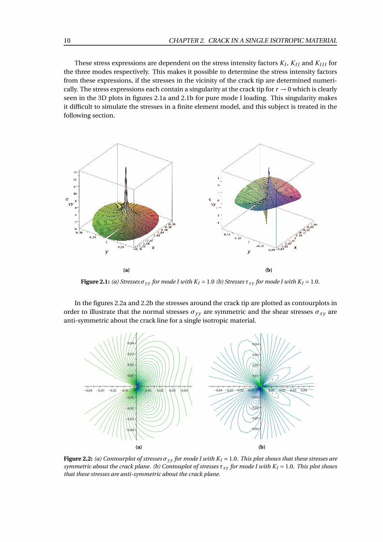
cally. The stress expressions each contain a singularity at the crack tip for r → 0 which is clearly
seen in the 3D plots in figures 2.1a and 2.1b for pure mode I loading. This singularity makes
it difficult to simulate the stresses in a finite element model, and this subject is treated in the
following section.
(a) (b)
Figure 2.1: (a) Stresses σy y for mode I with K I = 1.0 (b) Stresses τx y for mode I with K I = 1.0.
In the figures 2.2a and 2.2b the stresses around the crack tip are plotted as contourplots in
order to illustrate that the normal stresses σy y are symmetric and the shear stresses σx y are
anti-symmetric about the crack line for a single isotropic material.
(a) (b)
Figure 2.2: (a) Contourplot of stresses σy y for mode I with K I = 1.0. This plot shows that these stresses are
symmetric about the crack plane. (b) Contouplot of stresses τx y for mode I with K I = 1.0. This plot shows
that these stresses are anti-symmetric about the crack plane.
2.1. STRESSES AND DISPLACEMENTS AROUND A CRACK TIP 11
The displacements around the crack tip for the three fracture modes are (Kildegaard, 2002,
p. 27, 32, 38):
Mode I
[
u
v
]
=2(1+ν)
EK I
√
r
2π
cos θ2
[
κ−12
+sin2 θ2
]
sin θ2
[
κ+12 −cos2 θ
2
]
(2.4)
Mode II
[
u
v
]
=2(1+ν)
EK I I
√
r
2π
sin θ2
[
κ+12 −cos2 θ
2
]
cos θ2
[
κ−12
+sin2 θ2
]
(2.5)
Mode III
[
w]
= 41+ν
EK I I I
√
r
2π
[
sin θ2
]
(2.6)
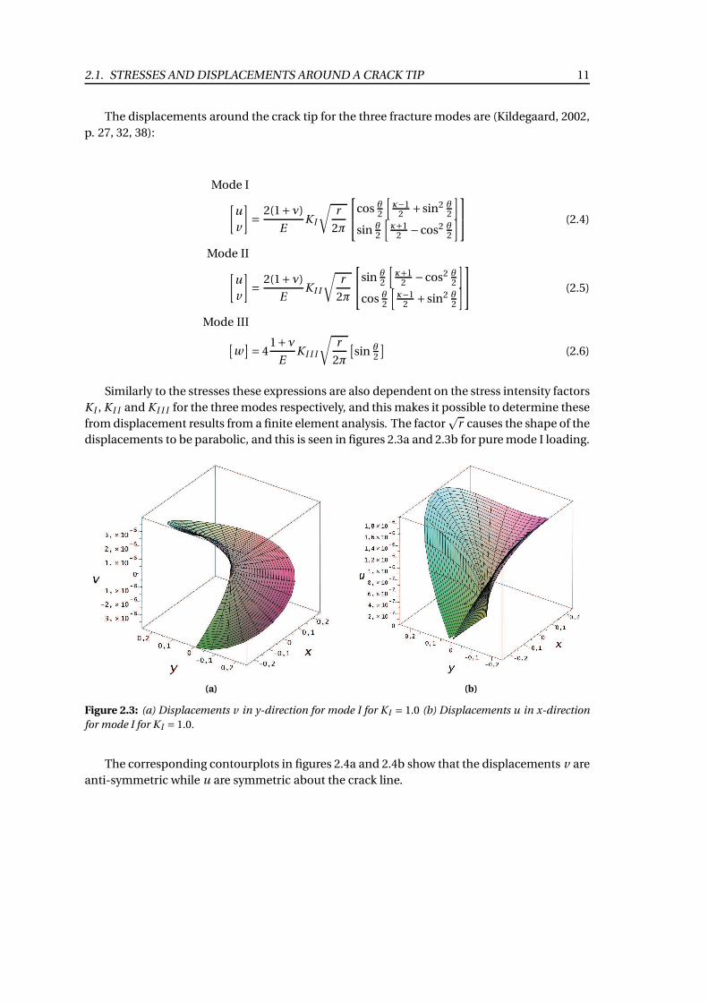
Similarly to the stresses these expressions are also dependent on the stress intensity factors
K I , K I I and K I I I for the three modes respectively, and this makes it possible to determine these
from displacement results from a finite element analysis. The factorp
r causes the shape of the
displacements to be parabolic, and this is seen in figures 2.3a and 2.3b for pure mode I loading.
(a) (b)
Figure 2.3: (a) Displacements v in y-direction for mode I for K I = 1.0 (b) Displacements u in x-direction
for mode I for K I = 1.0.
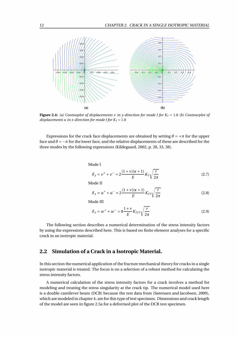
The corresponding contourplots in figures 2.4a and 2.4b show that the displacements v are
anti-symmetric while u are symmetric about the crack line.
12 CHAPTER 2. CRACK IN A SINGLE ISOTROPIC MATERIAL
(a) (b)
Figure 2.4: (a) Contouplot of displacements v in y-direction for mode I for K I = 1.0 (b) Contourplot of
displacements u in x-direction for mode I for K I = 1.0
Expressions for the crack face displacements are obtained by setting θ =+π for the upper
face and θ=−π for the lower face, and the relative displacements of these are described for the
three modes by the following expressions (Kildegaard, 2002, p. 28, 33, 38).
Mode I
δy = v++v− = 2(1+ν)(κ+1)
EK I
√
r
2π(2.7)
Mode II
δx = u++u− = 2(1+ν)(κ+1)
EK I I
√
r
2π(2.8)
Mode III
δz = w++w− = 81+ν
EK I I I
√
r
2π(2.9)
The following section describes a numerical determination of the stress intensity factors
by using the expressions described here. This is based on finite element analyses for a specific
crack in an isotropic material.
2.2 Simulation of a Crack in a Isotropic Material.
In this section the numerical application of the fracture mechanical theory for cracks in a single
isotropic material is treated. The focus is on a selection of a robust method for calculating the
stress intensity factors.
A numerical calculation of the stress intensity factors for a crack involves a method for
modeling and treating the stress singularity at the crack tip. The numerical model used here
is a double cantilever beam (DCB) because the test data from (Sørensen and Jacobsen, 2009),
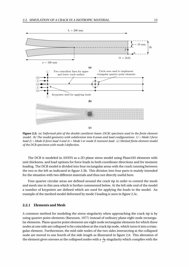
which are modeled in chapter 4, are for this type of test specimen. Dimensions and crack length
of the model are seen in figure 2.5a for a deformed plot of the DCB test specimen.
2.2. SIMULATION OF A CRACK IN A ISOTROPIC MATERIAL. 13
L = 200 mm
h = 10 mm2h
a = 100 mm
O = (0,0)
yx
(a)
Two coincident lines for upper
and lower crack surface
Circle area used to implement
triangular quarter point elements
Keypoints used for applying loads
1
3,4
2
2
3,4
3,4
1
(b)
(c)
Figure 2.5: (a) Deformed plot of the double cantilever beam (DCB) specimen used in the finite element
model. (b) The model geometry with subdivision into 8 areas and load configurations: 1) = Mode I force
load 2) = Mode II force load 3 and 4) = Mode I or mode II moment load. (c) Meshed finite element model
of the DCB specimen with mode I deflection.
The DCB is modeled in ANSYS as a 2D plane stress model using Plane183 elements with
unit thickness, and load options for force loads in both coordinate directions and for moment
loading. The DCB model is divided into four rectangular areas with the crack running between
the two to the left as indicated in figure 2.5b. This division into four parts is mainly intended
for the situation with two different materials and thus not directly useful here.
Four quarter circular areas are defined around the crack tip in order to control the mesh
and mesh size in this area which is further commented below. At the left side end of the model
a number of keypoints are defined which are used for applying the loads to the model. An
example of the meshed model deformed by mode I loading is seen in figure 2.5c.
2.2.1 Elements and Mesh
A common method for modeling the stress singularity when approaching the crack tip is by
using quarter point elements (Barsoum, 1977) instead of ordinary plane eight node rectangu-
lar elements. Plane quarter point elements are eight node rectangular elements for which three
nodes at one side are collapsed to be coincident at the crack tip node, which turns it into a trian-
gular element. Furthermore, the mid-side nodes of the two sides intersecting at the collapsed
node are moved to one fourth of the side length as illustrated in figure 2.6. This alteration of
the element gives stresses at the collapsed nodes with a 1pr
singularity which complies with the
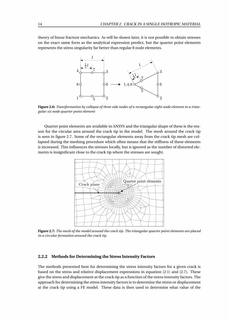
14 CHAPTER 2. CRACK IN A SINGLE ISOTROPIC MATERIAL
theory of linear fracture mechanics. As will be shown later, it is not possible to obtain stresses
on the exact same form as the analytical expression predict, but the quarter point elements
represents the stress singularity far better than regular 8 node elements.
3
21
4 7
8
5
6
5
7
1,4,8
3
6
2
12 l
l
14l
l
Figure 2.6: Transformation by collapse of three side nodes of a rectangular eight node element to a trian-
gular six node quarter point element
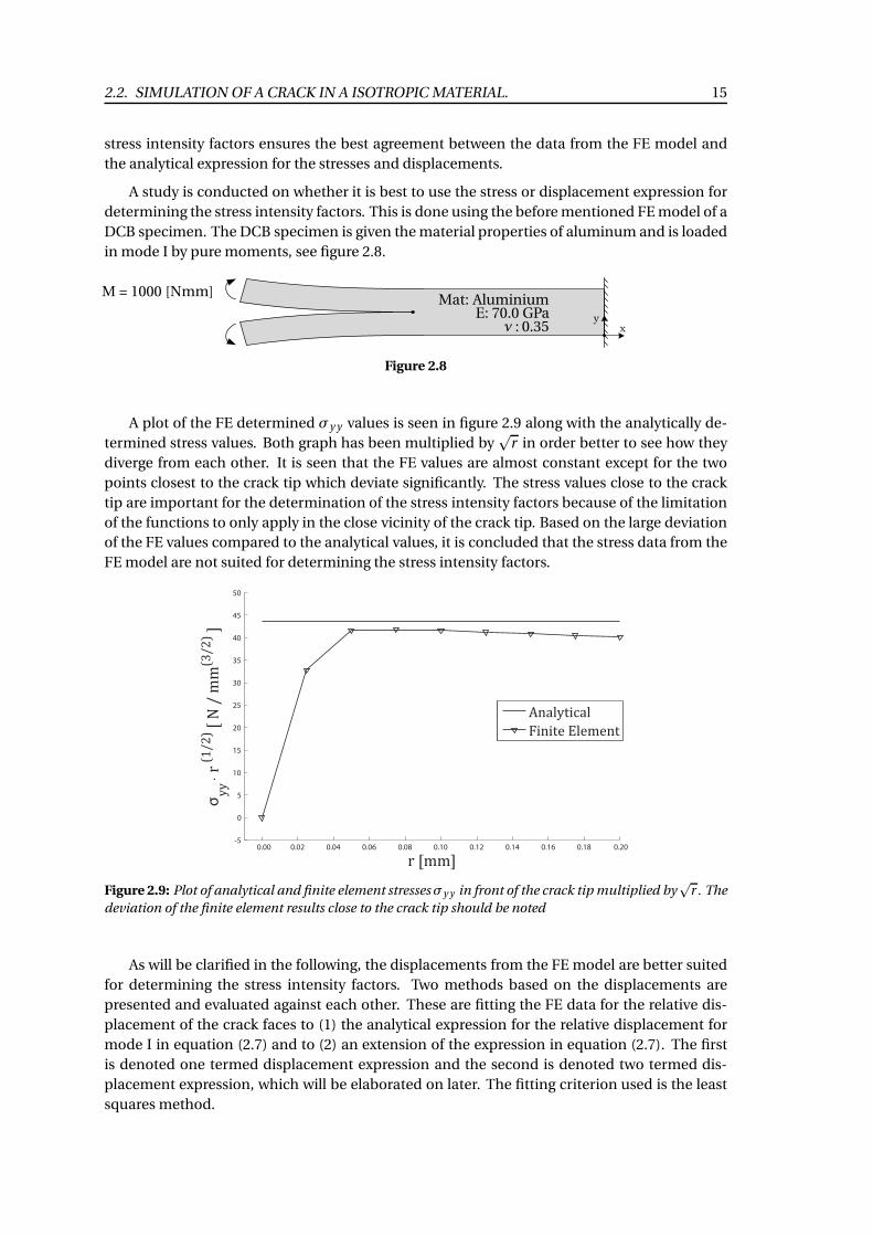
Quarter point elements are available in ANSYS and the triangular shape of these is the rea-
son for the circular area around the crack tip in the model. The mesh around the crack tip
is seen in figure 2.7. Some of the rectangular elements away from the crack tip mesh are col-
lapsed during the meshing procedure which often means that the stiffness of these elements
is increased. This influences the stresses locally, but is ignored as the number of distorted ele-
ments is insignificant close to the crack tip where the stresses are sought.
1
Quarter point elementsCrack plane
Figure 2.7: The mesh of the model around the crack tip. The triangular quarter point elements are placed
in a circular formation around the crack tip.
2.2.2 Methods for Determining the Stress Intensity Factors
The methods presented here for determining the stress intensity factors for a given crack is
based on the stress and relative displacement expressions in equation (2.1) and (2.7). These
give the stress and displacement at the crack tip as a function of the stress intensity factors. The
approach for determining the stress intensity factors is to determine the stress or displacement
at the crack tip using a FE model. These data is then used to determine what value of the
2.2. SIMULATION OF A CRACK IN A ISOTROPIC MATERIAL. 15
stress intensity factors ensures the best agreement between the data from the FE model and
the analytical expression for the stresses and displacements.
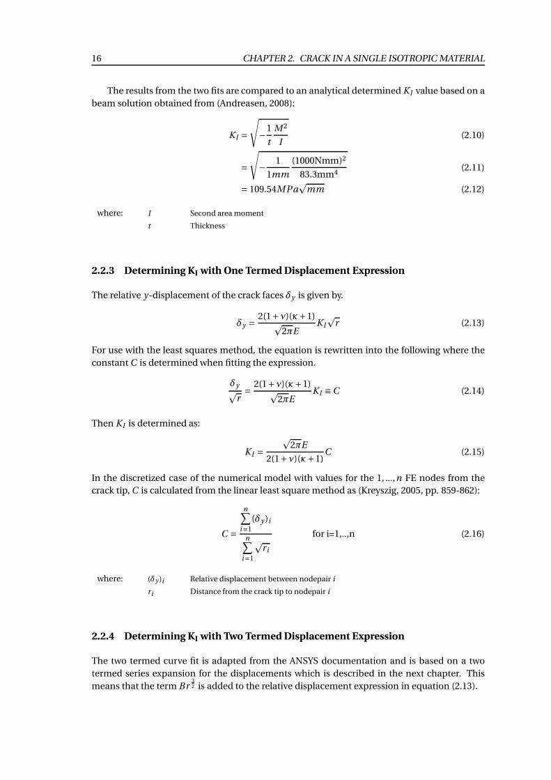
A study is conducted on whether it is best to use the stress or displacement expression for
determining the stress intensity factors. This is done using the before mentioned FE model of a
DCB specimen. The DCB specimen is given the material properties of aluminum and is loaded
in mode I by pure moments, see figure 2.8.
yx
Mat: AluminiumE: 70.0 GPa
ν : 0.35
M = 1000 [Nmm]
Figure 2.8
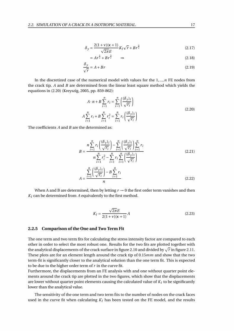
A plot of the FE determined σy y values is seen in figure 2.9 along with the analytically de-
termined stress values. Both graph has been multiplied byp
r in order better to see how they
diverge from each other. It is seen that the FE values are almost constant except for the two
points closest to the crack tip which deviate significantly. The stress values close to the crack
tip are important for the determination of the stress intensity factors because of the limitation
of the functions to only apply in the close vicinity of the crack tip. Based on the large deviation
of the FE values compared to the analytical values, it is concluded that the stress data from the
FE model are not suited for determining the stress intensity factors.
0.00 0.02 0.04 0.06 0.08 0.10 0.12 0.14 0.16 0.18 0.20-5
0
5
10
15
20
25
30
35
40
45
50
r [mm]
σy
y
r(1
/2
) [ N
/ m
m(3
/2
) ]
Analytical
Finite Element
∙
Figure 2.9: Plot of analytical and finite element stresses σy y in front of the crack tip multiplied byp
r . The
deviation of the finite element results close to the crack tip should be noted
As will be clarified in the following, the displacements from the FE model are better suited
for determining the stress intensity factors. Two methods based on the displacements are
presented and evaluated against each other. These are fitting the FE data for the relative dis-
placement of the crack faces to (1) the analytical expression for the relative displacement for
mode I in equation (2.7) and to (2) an extension of the expression in equation (2.7). The first
is denoted one termed displacement expression and the second is denoted two termed dis-
placement expression, which will be elaborated on later. The fitting criterion used is the least
squares method.
16 CHAPTER 2. CRACK IN A SINGLE ISOTROPIC MATERIAL
The results from the two fits are compared to an analytical determined K I value based on a
beam solution obtained from (Andreasen, 2008):
K I =
√
−1
t
M 2
I(2.10)
=
√
−1
1mm
(1000Nmm)2
83.3mm4(2.11)
= 109.54MPap
mm (2.12)
where: I Second area moment
t Thickness
2.2.3 Determining KI with One Termed Displacement Expression
The relative y-displacement of the crack faces δy is given by.
δy =2(1+ν)(κ+1)
p2πE
K I
pr (2.13)
For use with the least squares method, the equation is rewritten into the following where the
constant C is determined when fitting the expression.
δypr=
2(1+ν)(κ+1)p
2πEK I ≡C (2.14)
Then K I is determined as:
K I =p
2πE
2(1+ν)(κ+1)C (2.15)
In the discretized case of the numerical model with values for the 1, ...,n FE nodes from the
crack tip, C is calculated from the linear least square method as (Kreyszig, 2005, pp. 859-862):
C =
n∑
i=1
(δy )i
n∑
i=1
pri
for i=1,..,n (2.16)
where: (δy )i Relative displacement between nodepair i
ri Distance from the crack tip to nodepair i
2.2.4 Determining KI with Two Termed Displacement Expression
The two termed curve fit is adapted from the ANSYS documentation and is based on a two
termed series expansion for the displacements which is described in the next chapter. This
means that the term Br32 is added to the relative displacement expression in equation (2.13).
2.2. SIMULATION OF A CRACK IN A ISOTROPIC MATERIAL. 17
δy =2(1+ν)(κ+1)
p2πE
K I
pr +Br
32 (2.17)
= Ar12 +Br
32 ⇒ (2.18)
δypr= A+Br (2.19)
In the discretized case of the numerical model with values for the 1, ...,n FE nodes from
the crack tip, A and B are determined from the linear least square method which yields the
equations in (2.20) (Kreyszig, 2005, pp. 859-862):
A ·n +Bn∑
i=1
ri =n∑
i=1
(
(δy )ip
ri
)
An∑
i=1
ri +Bn∑
i=1
r 2i =
n∑
i=1
ri
(
(δy )ip
ri
)
(2.20)
The coefficients A and B are the determined as:
B =n
n∑
i=1
ri
(
(δy )ip
ri
)
−n∑
i=1
(
(δy )ip
ri
) n∑
i=1
ri
nn∑
i=1
r 2i −
n∑
i=1
ri
n∑
i=1
(
(δy )ip
ri
)(2.21)
A =
n∑
i=1
(
(δy )ip
ri
)
−Bn∑
i=1
ri
n(2.22)
When A and B are determined, then by letting r → 0 the first order term vanishes and then
K I can be determined from A equivalently to the first method.
K I =p
2πE
2(1+ν)(κ+1)A (2.23)
2.2.5 Comparison of the One and Two Term Fit
The one term and two term fits for calculating the stress intensity factor are compared to each
other in order to select the most robust one. Results for the two fits are plotted together with
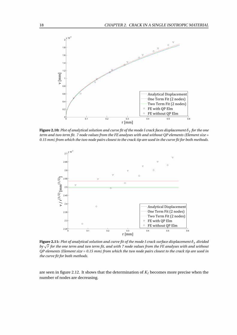
the analytical displacements of the crack surface in figure 2.10 and divided byp
r in figure 2.11.
These plots are for an element length around the crack tip of 0.15mm and show that the two
term-fit is significantly closer to the analytical solution than the one term fit. This is expected
to be due to the higher order term of r in the curve fit.
Furthermore, the displacements from an FE analysis with and one without quarter point ele-
ments around the crack tip are plotted in the two figures, which show that the displacements
are lower without quarter point elements causing the calculated value of K I to be significantly
lower than the analytical value.
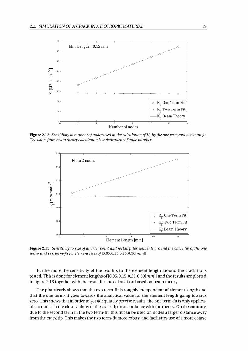
The sensitivity of the one term and two term fits to the number of nodes on the crack faces
used in the curve fit when calculating K I has been tested on the FE model, and the results
18 CHAPTER 2. CRACK IN A SINGLE ISOTROPIC MATERIAL
0 0.1 0.2 0.3 0.4 0.5 0.60
0.2
0.4
0.6
0.8
1
1.2
1.4
1.6
1.8
2x 10
-3
!"##$
%!"#
#$
&'()*+,-()!.,/0)(-1#1'+
2'1!31 #!4,+!56!'781/9
3:7!31 #!4,+!56!'781/9
4;!:,+<!=>!;)#
4;!:,+<7?+!=>!;)#
Figure 2.10: Plot of analytical solution and curve fit of the mode I crack faces displacement δy for the one
term and two term fit. 7 node values from the FE analyses with and without QP elements (Element size =
0.15 mm) from which the two node pairs closest to the crack tip are used in the curve fit for both methods.
0 0.1 0.2 0.3 0.4 0.5 0.62.25
2.3
2.35
2.4
2.45
2.5
2.55
2.6
2.65
2.7x 10
-3
!"##$
%!&! '(
&)* !"#
#'(
&)* $
+,-./012-.!3145.-26#6,0
7,6!86 #!910!')!,:;64*
8<:!86 #!910!')!,:;64*
9=!<10>!?@!=.#
9=!<10>:A0!?@!=.#
Figure 2.11: Plot of analytical solution and curve fit of the mode I crack surface displacement δy divided
byp
r for the one term and two term fit, and with 7 node values from the FE analyses with and without
QP elements (Element size = 0.15 mm) from which the two node pairs closest to the crack tip are used in
the curve fit for both methods.
are seen in figure 2.12. It shows that the determination of K I becomes more precise when the
number of nodes are decreasing.
2.2. SIMULATION OF A CRACK IN A ISOTROPIC MATERIAL. 19
0 2 4 6 8 10 12 14104
106
108
110
112
114
116
118
120
!"#$%&'(&)'*$+
,-&./01&""2345
67"8&9$):;<&=&>82?&""
,-@&A)$&B$%"&CD;
,-@&BE'&B$%"&CD;
,-@&F$1"&B<$'%G
Figure 2.12: Sensitivity to number of nodes used in the calculation of K I by the one term and two term fit.
The value from beam theory calculation is independent of node number.
0 0.1 0.2 0.3 0.4 0.5104
106
108
110
112
114
116
!"#"$%&'"$(%)&*##+
,-&*.
/0&##123+
45%&%6&3&$67"8
,-9&:$"&;"<#&45%
,-9&;=6&;"<#&45%
,-9&>"0#&;)"6<?
Figure 2.13: Sensitivity to size of quarter point and rectangular elements around the crack tip of the one
term- and two term-fit for element sizes of [0.05,0.15,0.25,0.50[mm]].
Furthermore the sensitivity of the two fits to the element length around the crack tip is
tested. This is done for element lengths of [0.05,0.15,0.25,0.50[mm]] and the results are plotted
in figure 2.13 together with the result for the calculation based on beam theory.
The plot clearly shows that the two term-fit is roughly independent of element length and
that the one term-fit goes towards the analytical value for the element length going towards
zero. This shows that in order to get adequately precise results, the one term-fit is only applica-
ble to nodes in the close vicinity of the crack tip in accordance with the theory. On the contrary,
due to the second term in the two term-fit, this fit can be used on nodes a larger distance away
from the crack tip. This makes the two term-fit more robust and facilitates use of a more coarse

20 CHAPTER 2. CRACK IN A SINGLE ISOTROPIC MATERIAL
mesh that still gives satisfactory results. Because of this, the two term-fit is considered most
suitable for the calculation and is chosen as the method to be used further on in the report.
The two curve fit methods have been tested and compared for mode II with the same conclu-
sions.
Chapter
3Interface Crack between Two IsotropicMaterials
The purpose of this chapter is to derive and explain the complete expressions for the stresses and
displacements at the crack tip of an interface crack between two dissimilar isotropic materials.
Furthermore, the energy release rate as a function of the complex stress intensity factor is given as
a function of the stress intensity factors. The expressions for the relative crack surface displace-
ments are applied in a simulation of a crack between to dissimilar isotropic materials where
different studies are conducted on how to determine the stress intensity factors and the energy
release rate.
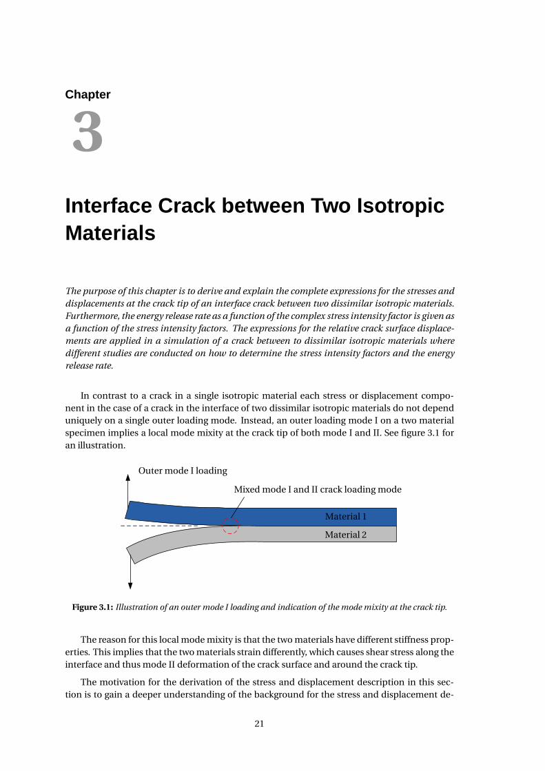
In contrast to a crack in a single isotropic material each stress or displacement compo-
nent in the case of a crack in the interface of two dissimilar isotropic materials do not depend
uniquely on a single outer loading mode. Instead, an outer loading mode I on a two material
specimen implies a local mode mixity at the crack tip of both mode I and II. See figure 3.1 for
an illustration.
Mixed mode I and II crack loading mode
Outer mode I loading
Material 1
Material 2
Figure 3.1: Illustration of an outer mode I loading and indication of the mode mixity at the crack tip.
The reason for this local mode mixity is that the two materials have different stiffness prop-
erties. This implies that the two materials strain differently, which causes shear stress along the
interface and thus mode II deformation of the crack surface and around the crack tip.
The motivation for the derivation of the stress and displacement description in this sec-
tion is to gain a deeper understanding of the background for the stress and displacement de-
21
22 CHAPTER 3. INTERFACE CRACK BETWEEN TWO ISOTROPIC MATERIALS
scription for an interface crack between two dissimilar isotropic materials described in article
(Suo and Hutchinson, 1990). In this article the stress and displacement are given for the crack
interface (θ = 0), only.
Although the stress or displacement description at the interface is sufficient for determin-
ing the stress intensity factors by numeric simulation, the full field solutions for stresses and
displacements around the crack tip are considered relevant to obtain. This is seen in the per-
spective of achieving a wide comprehension of the stresses and displacements at an interfacial
crack tip and mathematical method used for describing them.
Furthermore, it has only been possible to obtain the first eigenfunction expressions for
the stresses and displacements for the interface between the two materials from the article
(Suo and Hutchinson, 1990). This means that these expressions are only valid very close to the
crack tip and not suited for use with the FE analysis for determination of the stress intensity
factors that must be conducted because this calls for very small elements in the model. Hence,
the rest of the terms in the series describing the stresses and displacements are derived here.
The approach when dealing with interface cracks between two dissimilar isotropic mate-
rials and the idea of terms like the bimaterial constant and oscillating singularities, which are
treated later in this chapter, are equivalent to the ideas and terms figuring in the more general
description of an interfacial crack between anisotropic materials which are treated in chapter
4. Therefore a thorough treatment of these terms and ideas are presented here both for use in
the simulation of a crack between two dissimilar isotropic materials as well as a basis for the
theory presented in chapter 4.
3.1 Theory of Interfacial Crack Between Two Isotropic Materials
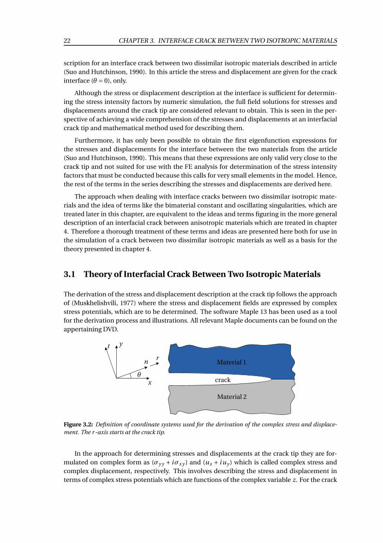
The derivation of the stress and displacement description at the crack tip follows the approach
of (Muskhelishvili, 1977) where the stress and displacement fields are expressed by complex
stress potentials, which are to be determined. The software Maple 13 has been used as a tool
for the derivation process and illustrations. All relevant Maple documents can be found on the
appertaining DVD.
θ
n
y
x
t
r
crack
Material 1
Material 2
Figure 3.2: Definition of coordinate systems used for the derivation of the complex stress and displace-
ment. The r -axis starts at the crack tip.
In the approach for determining stresses and displacements at the crack tip they are for-
mulated on complex form as (σy y + iσx y ) and (ux + i uy ) which is called complex stress and
complex displacement, respectively. This involves describing the stress and displacement in
terms of complex stress potentials which are functions of the complex variable z. For the crack

3.1. THEORY OF INTERFACIAL CRACK BETWEEN TWO ISOTROPIC MATERIALS 23
illustrated in figure 3.2 the following complex displacement is given (Rathkjen, 1984, p. 33).
ux + i uy =1
2µ j
(
κ j ·φ(z)− z ·Φ(z)−ψ(z))
(3.1)
where: φ(z) Complex stress potential
ψ(z) Complex stress potential
Φ(z) Complex stress potential defined as ddz
φ(z)
µ Shear module
κ Poisson parameter for plane stress or strain
j Index for material 1 or material 2
In the same way the so called fundamental stress combinations expressed by stress poten-
tials in cartesian coordinates are given as (Rathkjen, 1984, p. 27).
σxx +σy y = 2(
Φ(z)+Φ(z))
(3.2)
σy y −σxx +2iσx y = 2
(
z
(
d
dzΦ(z)
)
+Ψ(z)
)
(3.3)
where: Ψ(z) Complex stress potential defined as ddz
ψ(z)
The sum of these fundamental stress combinations eliminates σxx and yields the follow-
ing complex expression for the σy y and σx y which are of interest for the stress analysis at the
crack tip, because these stresses are the only stresses that influence the propagation of a crack
orientated as in figure 3.2.
σy y + iσx y =Φ(z)+Φ(z)+ z
(
d
dzΦ(z)
)
+Ψ(z) (3.4)
In order to obtain the complex stress and complex displacement the task is to determine
the stress potentials. To do this the complex stress and complex displacement are transformed
to a nt -coordinate system that is rotated θ in relation to the x y-coordinate system, see figure
3.2. This is partly due to the way these types of problems has been solved in the past and
because it makes it possible to solve for wedge formed crack geometries instead of closed crack
geometries which in the end, though, are treated in the present derivation.
The complex stress and displacement transformed to the nt -system expressed by stress
potentials are given as (Rathkjen, 1984, p.33):
σt t + iσnt =Φ(z)+Φ(z)+(
z
(
d
dzΦ(z)
)
+Ψ(z)
)
e2iθ (3.5)
un + i ut =1
2µ
(
κ j ·φ(z)− z ·Φ(z)−ψ(z))
e−iθ (3.6)
The complex stress and displacement in the nt -coordinates (3.5) and (3.6) are used to
determine the stress potentials figuring in the complex stress and displacement in equation
(3.1) and (3.4). This is done by applying the boundary conditions for the stresses on the crack
faces and behind the crack tip, and boundary conditions for the displacement across the inter-
face. The boundary conditions are described in section 3.1.1 With these boundary conditions
24 CHAPTER 3. INTERFACE CRACK BETWEEN TWO ISOTROPIC MATERIALS
around the crack tip in mind the stress potentials are guessed to be in the form showed in the
following equations (Williams, 1959, p. 200):
φ j (z) = A j zλ+iε+B j zλ−iε (3.7)
ψ j (z) =C j zλ+iε+D j zλ−iε (3.8)
Φ j (z) =d
dzφ j =
A j zλ+iε (λ+ iε)
z+
B j zλ−iε (λ− iε)
z(3.9)
Ψ j (z) =d
dzψ j =
C j zλ+iε (λ+ iε)
z+
D j zλ−iε (λ− iε)
z(3.10)
where: A j ,B j ,C j ,D j Complex material parameters
λ Singularity parameter
ε Bimaterial constant
The reason that the stress potentials are guessed to be in this form is that they have the
ability to produce the stress singularity at the crack tip from the power of the real number λ as
zλ+iε = r λ+iεe iθ(λ+iε) and the denominator, z in the Φ and Ψ stress potentials. In addition this
form of the stress potentials shows a discontinuity across the crack surfaces as θ is uniquely
defined in the interval [−π,π] only. Thus when going from the upper crack surface to the lower,
θ changes from +π to −π (see figure 3.3).
The following part of the derivation concerns a verification showing that stress potentials
on this form are applicable and a determination of the constants figuring in the stress poten-
tials as well as a solution for λ and ε.
By inserting the stress potentials Ψ j and Φ j into (3.5) and by converting the complex vari-
able z to polar form as z = r e iθ and zλ+iε = r λ+iεe iθ(λ+iε) the complex stress in nt -coordinates
is expressed as:
σt t + iσnt =1
r 1−λ
([
(λ+ iε)2 e iθ(λ+iε−1)A j + (λ− iε)2 e iθ(λ−iε−1)B j
+ (λ+ iε)e iθ(λ+iε)e iθC j + (λ− iε) e iθ(λ−iε)e iθD j
+ (λ− iε)e−iθ(λ−iε+1) A j + (λ+ iε) e−iθ(λ+iε+1)B j
]
cos(ln(r )ε)
+ i
[
(λ+ iε)2 e iθ(λ+iε−1)A j − (λ− iε)2 e iθ(λ−iε−1)B j
+ (λ+ iε)e iθ(λ+iε)e iθC j − (λ− iε) e iθ(λ−iε)e iθD j
− (λ− iε)e−iθ(λ−iε+1) A j + (λ+ iε) e−iθ(λ+iε+1)B j
]
sin(ln(r )ε)
)
(3.11)
The cosine and sine terms in equation (3.11) emerges from r iε = e i (ln(r )ε) = cos(ln(r )ε)+i sin(ln(r )ε) and cause a so-called oscillating singularity to the stress description for r → 0. It
should be noted in equation (3.11) that the polar representation uses the same angle θ as is
used in the coordinate transformation from the x y-system to the nt -system. This implies that
a chosen point z = r e iθ always lies on the n-axis.
3.1. THEORY OF INTERFACIAL CRACK BETWEEN TWO ISOTROPIC MATERIALS 25
In the same manner as for the complex stress the complex displacement from equation
(3.6) is expressed as:
un + i ut =r λ
e iθ·
1
2µ j·([
κ j
(
A j e iθ(λ+iε)−B j e iθ(λ−iε)
)
+ A j e i 2θe−iθ(λ−iε)(λ− iε)−B j e i 2θe−iθ(λ+iε)(λ+ iε)
+C j e−iθ(λ−iε)−D j e−iθ(λ+iε)
]
i sin(ln(r )ε)
+[
κ j
(
A j e iθ(λ+iε)+B j e iθ(λ−iε)
)
− A j e i 2θe−iθ(λ−iε)(λ− iε)−B j e i 2θe−iθ(λ+iε)(λ+ iε)
−C j e−iθ(λ−iε)−D j e−iθ(λ+iε)
]
cos(ln(r )ε)
)
(3.12)
It is seen that the expression for the complex displacement consists of an oscillating sine
and cosine term similar to the complex stress.
3.1.1 Applying the Boundary Conditions
It is assumed that boundaries other than the crack faces and the unbroken interface between
the two materials can be ignored because a solution is sought in the close vicinity of the crack
tip only. In this way the outer geometry of a given structure does not influence the solution.
As will be shown later the outer geometry and external load are accounted for in the complex
stress intensity factor K = K I +i K I I . The boundary conditions for the crack faces and the inter-
face are illustrated in figure 3.3 and given as:
1. No stresses on the crack faces for material 1 and 2.
2. Continuity of σx y and σy y across the interface between material 1 and 2.
3. Continuity of ux and uy across the interface between material 1 and 2.
These boundary conditions are used in the following to determine the parameters A1, ...,D2.
This results in an eigenvalue problem with a system of 8 equations.
Applying boundary condition 1 The C1 and D1 coefficients of the complex stress potentials
for material 1 are obtained by applying the boundary conditions of item 1 in the list above.
For the complex stress component on the crack faces to equal zero for material 1, that is σy y +iσx y = 0 at θ = π, the coefficients of the cosine and sine terms in equations (3.11) must equal
zero. From the cosine term C1 (A1,B1) is obtained and from the sine term the expression for
D1 (A1,B1,C1) is obtained. C2 (A2,B2) and D2 (A2,B2,C2) are obtained similarly for σy y +iσx y =0 at θ =−π.
Applying boundary condition 2 The A2 and B2 coefficients are obtained by applying the
boundary conditions of item 2. In order for the stresses to be continuous across the interface
26 CHAPTER 3. INTERFACE CRACK BETWEEN TWO ISOTROPIC MATERIALS
θ
−θ
θ =±π
σy y (θ =π) = 0
σx y (θ =π) = 0
σy y (θ =−π) = 0
σx y (θ =−π) = 0
σy y,1(θ = 0) =σy y,2(θ = 0)
σx y,1(θ = 0) =σx y,2(θ = 0)
ux,1(θ = 0) = ux,2(θ = 0)
uy,1(θ = 0) = uy,2(θ = 0)
x
y
Material 1
Material 2
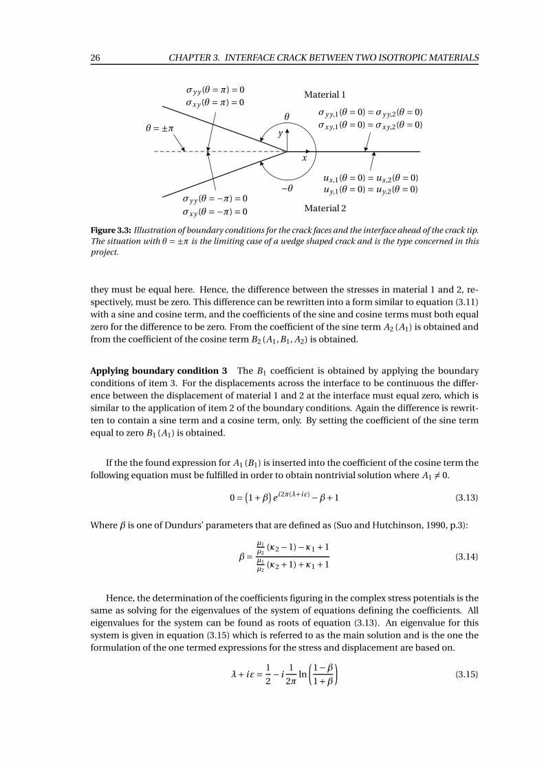
Figure 3.3: Illustration of boundary conditions for the crack faces and the interface ahead of the crack tip.
The situation with θ = ±π is the limiting case of a wedge shaped crack and is the type concerned in this
project.
they must be equal here. Hence, the difference between the stresses in material 1 and 2, re-
spectively, must be zero. This difference can be rewritten into a form similar to equation (3.11)
with a sine and cosine term, and the coefficients of the sine and cosine terms must both equal
zero for the difference to be zero. From the coefficient of the sine term A2 (A1) is obtained and
from the coefficient of the cosine term B2 (A1,B1, A2) is obtained.
Applying boundary condition 3 The B1 coefficient is obtained by applying the boundary
conditions of item 3. For the displacements across the interface to be continuous the differ-
ence between the displacement of material 1 and 2 at the interface must equal zero, which is
similar to the application of item 2 of the boundary conditions. Again the difference is rewrit-
ten to contain a sine term and a cosine term, only. By setting the coefficient of the sine term
equal to zero B1 (A1) is obtained.
If the the found expression for A1 (B1) is inserted into the coefficient of the cosine term the
following equation must be fulfilled in order to obtain nontrivial solution where A1 6= 0.
0 =(
1+β)
e i 2π(λ+iε)−β+1 (3.13)
Where β is one of Dundurs’ parameters that are defined as (Suo and Hutchinson, 1990, p.3):
β=µ1
µ2(κ2 −1)−κ1 +1
µ1
µ2(κ2 +1)+κ1 +1
(3.14)
Hence, the determination of the coefficients figuring in the complex stress potentials is the
same as solving for the eigenvalues of the system of equations defining the coefficients. All
eigenvalues for the system can be found as roots of equation (3.13). An eigenvalue for this
system is given in equation (3.15) which is referred to as the main solution and is the one the
formulation of the one termed expressions for the stress and displacement are based on.
λ+ iε=1
2− i
1
2πln
(
1−β
1+β
)
(3.15)
3.1. THEORY OF INTERFACIAL CRACK BETWEEN TWO ISOTROPIC MATERIALS 27
All other eigenvalues for this problem are given as:
λ+ iε=(1+2k)
2− i
1
2πln
(
1−β
1+β
)
where k ∈Z (3.16)
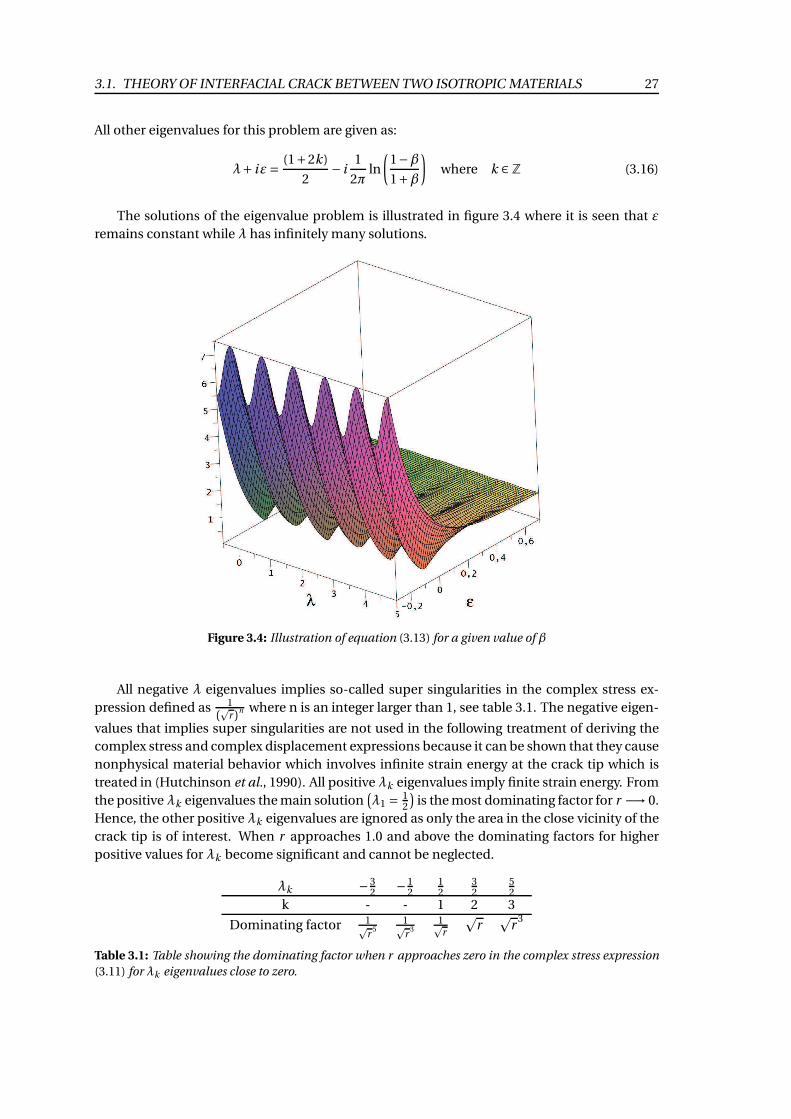
The solutions of the eigenvalue problem is illustrated in figure 3.4 where it is seen that ε
remains constant while λ has infinitely many solutions.
Figure 3.4: Illustration of equation (3.13) for a given value of β
All negative λ eigenvalues implies so-called super singularities in the complex stress ex-
pression defined as 1
(p
r )n where n is an integer larger than 1, see table 3.1. The negative eigen-
values that implies super singularities are not used in the following treatment of deriving the
complex stress and complex displacement expressions because it can be shown that they cause
nonphysical material behavior which involves infinite strain energy at the crack tip which is
treated in (Hutchinson et al., 1990). All positive λk eigenvalues imply finite strain energy. From
the positive λk eigenvalues the main solution(
λ1 = 12
)
is the most dominating factor for r −→ 0.
Hence, the other positive λk eigenvalues are ignored as only the area in the close vicinity of the
crack tip is of interest. When r approaches 1.0 and above the dominating factors for higher
positive values for λk become significant and cannot be neglected.
λk −32
−12
12
32
52
k - - 1 2 3
Dominating factor 1pr
51pr
31pr
pr
pr
3
Table 3.1: Table showing the dominating factor when r approaches zero in the complex stress expression
(3.11) for λk eigenvalues close to zero.
28 CHAPTER 3. INTERFACE CRACK BETWEEN TWO ISOTROPIC MATERIALS
As discovered in the simulation of a crack in a single isotropic material in chapter 2 there is
in some cases reason for including the next eigenvalue in the complex stress or displacement
description in order to utilize the use of larger elements at the crack tip while still being able to
obtain good estimates of the stress intensity factors. Hence, the displacement expression to be
used in the curve fit for determining the stress intensity factor for an interface crack must also
contain terms for the first and the second positive eigenvalue.
In order to fit the numerical results to the analytical solution containing these terms it is in
principle necessary just to know the dominating factor for the second eigenvalue term and not
the coefficient. For the first eigenvalue term though, the dominating factor and coefficient of
the main eigenvalue must be known. This is because the stress intensity factors can be calcu-
lated from the coefficient of the main dominating factor alone.
By inserting the eigenvalues λk and ε into the seven coefficients A2, B1, B2, C1, C2, D1
and D2 determined from solving the equations obtained from the boundary conditions they
reduce significantly which simplifies the expression for the complex stress and displacement.
The reduced coefficients are:
A2 =1−β
1+βA1 (3.17)
B1 = 0 (3.18)
B2 = 0 (3.19)
C1 =−(λk + iε) A1 (3.20)
C2 =−1−β
1+β(λk + iε) A1 (3.21)
D1 =1−β
1+βA1 (3.22)
D2 = A1 (3.23)
From the complex stress equation (3.4) the following eigenfunctions describing the com-
plex stress σ(λk ) is obtained by inserting the above coefficients.
σ(λk )=1
r λk
(
r iε ·Kp
2πc (1)+
r−iε ·Kp
2πc (2)
)
(3.24)
where: K Complex stress intensity factor (K I + i K I I )
k Index for eigenvalue: 0 = main eigenvalue, 1 = second eigenvalue,...
The coefficients c (1) and c (2) are given by:
c (1) =−1
2(1+β)(λk − iε−1)e iθ(λk+iε) ·
(
e−3iθ−e−iθ)
(3.25)
c (2) =1
2
(
(1+β) ·e iθ(−λk+iε+1)+ (1−β) ·e−iθ(−λk+iε+1))
(3.26)
The eigenfunction series describing the complex stress is then given as a linear combina-
tion of the eigenfunctions.
σy y + iσx y = 1.0 ·σ(
λ1 =1
2
)
+q1 ·σ(
λ2 =3
2
)
+q2 ·σ(
λ3 =5
2
)
+ ... (3.27)
3.1. THEORY OF INTERFACIAL CRACK BETWEEN TWO ISOTROPIC MATERIALS 29
where: q1 , q2 Weighting factors
The reason that the weight in front of the first eigenfunction is 1.0 is because consistency is
sought between the way the stress intensity factors are defined for a single isotropic material. In
this way the expression in equation (3.49) reduce to the stress description for a single isotropic
material if material properties are the same for material 1 and 2.
From comparing equation (3.24) for any specific value of λk and equation (3.4) with the
determined stress potentials inserted the complex stress intensity factor is determined to be:
A1,k =K (1+β)
2(λk − iε)p
2π(3.28)
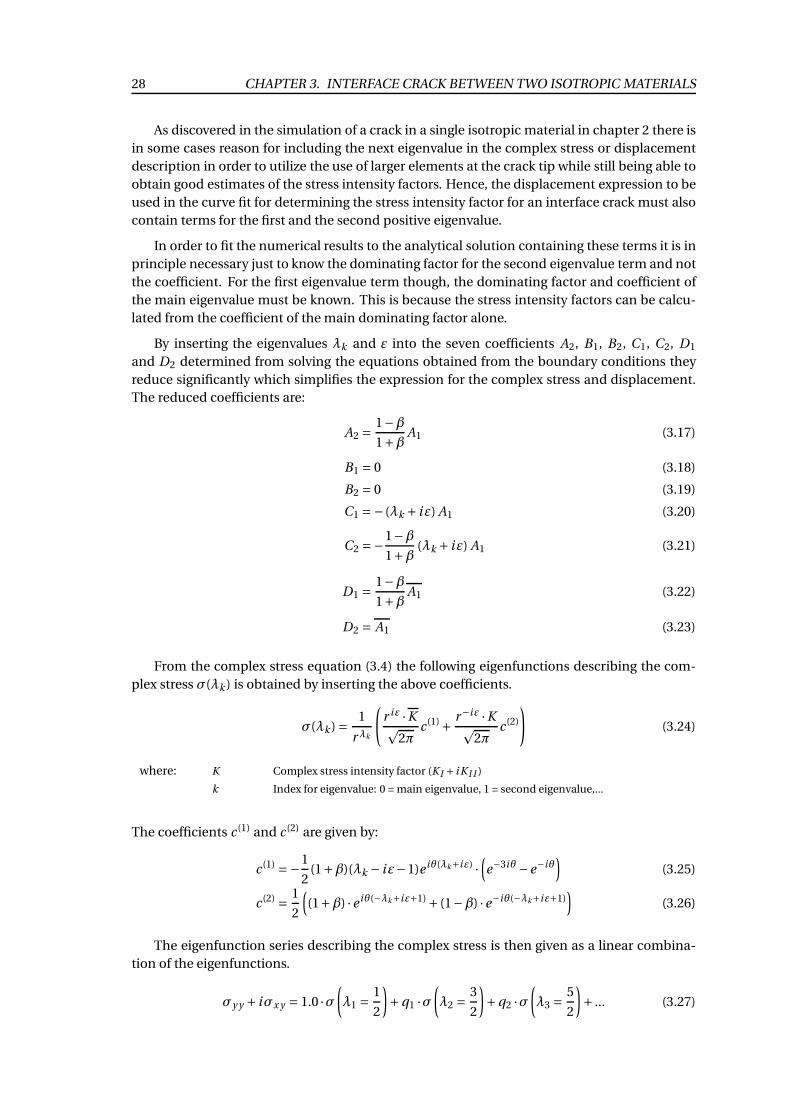
The stress components σy y andσx y are plotted in 3D in figure 3.5 as the real and imaginary
part of equation (3.49) for arbitrary chosen K = 83.3+i 76.3 and the material properties given in
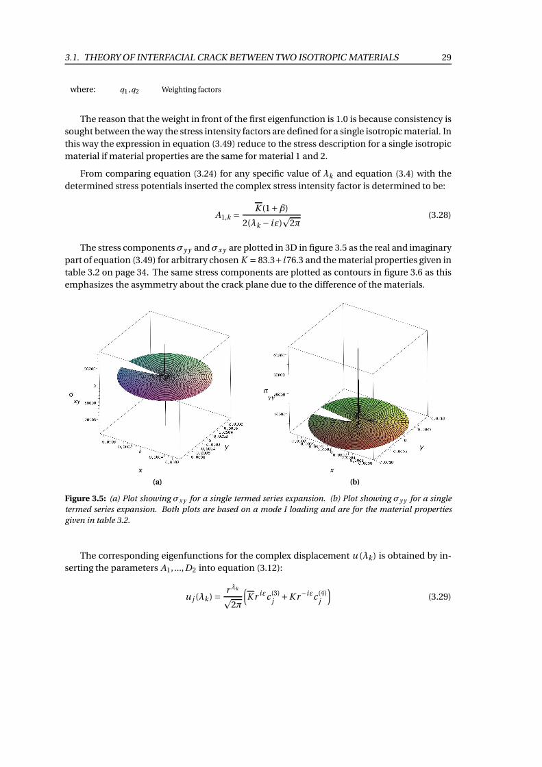
table 3.2 on page 34. The same stress components are plotted as contours in figure 3.6 as this
emphasizes the asymmetry about the crack plane due to the difference of the materials.
(a) (b)
Figure 3.5: (a) Plot showing σx y for a single termed series expansion. (b) Plot showing σy y for a single
termed series expansion. Both plots are based on a mode I loading and are for the material properties
given in table 3.2.
The corresponding eigenfunctions for the complex displacement u (λk ) is obtained by in-
serting the parameters A1, ...,D2 into equation (3.12):
u j (λk ) =r λk
p2π
(
K r iεc (3)j
+K r−iεc (4)j
)
(3.29)
30 CHAPTER 3. INTERFACE CRACK BETWEEN TWO ISOTROPIC MATERIALS
(a) (b)
Figure 3.6: (a) Contourplot of σx y for a single termed series expansion. (b) Contourplot of σy y for a single
termed series expansion. Both plots are based on a mode I loading and are for the material properties
given in table 3.2, and it is seen that the compared with the analogous plot for the single isotropic material
case, σx y is not anti-symmetric and σy y is not symmetric about the crack plane.
with the coefficients c (3)j
and c (4)j
being:
c (3)1 =
(
1+β)
·e iθλk ·e−θ·εκ1 − (1−β)e−iθλ ·eθ·ε
4(λk + iε)µ1(3.30)
c (3)2 =
(
1−β)
·e iθλk ·e−θ·εκ2 − (1+β)e−iθλ ·eθ·ε
4(λk + iε)µ2(3.31)
c (4)1 =
1
4µ1
(
1+β)
·e−iθλk ·e−θ·ε(1−e2iθ) (3.32)
c (4)2 =
1
4µ2
(
1−β)
·e−iθλk ·e−θ·ε(1−e2iθ) (3.33)
The eigenfunction series describing the complex displacement is then given as
ux + i uy = 1 ·u
(
λ1 =1
2
)
+q1 ·u
(
λ2 =3
2
)
+q2 ·u
(
λ3 =5
2
)
+ ... (3.34)
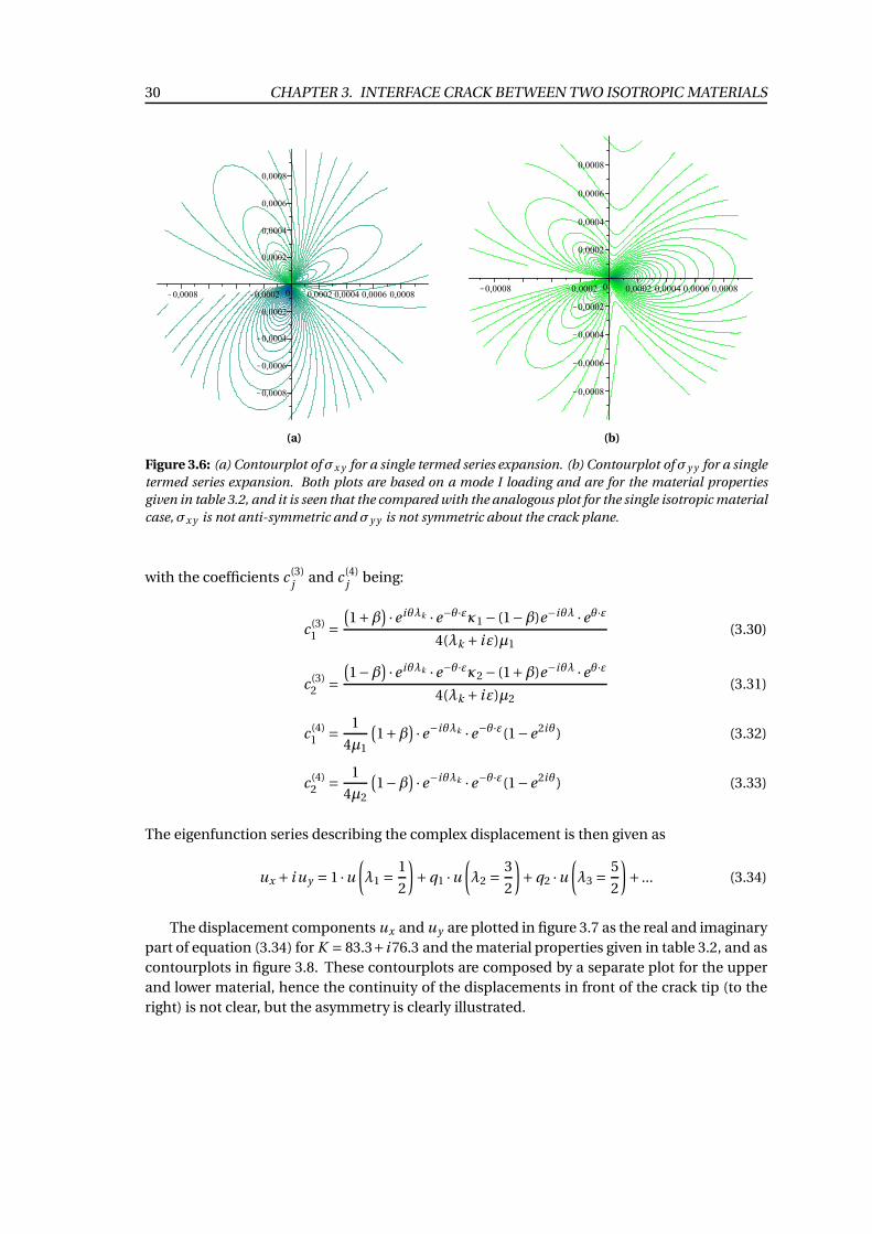
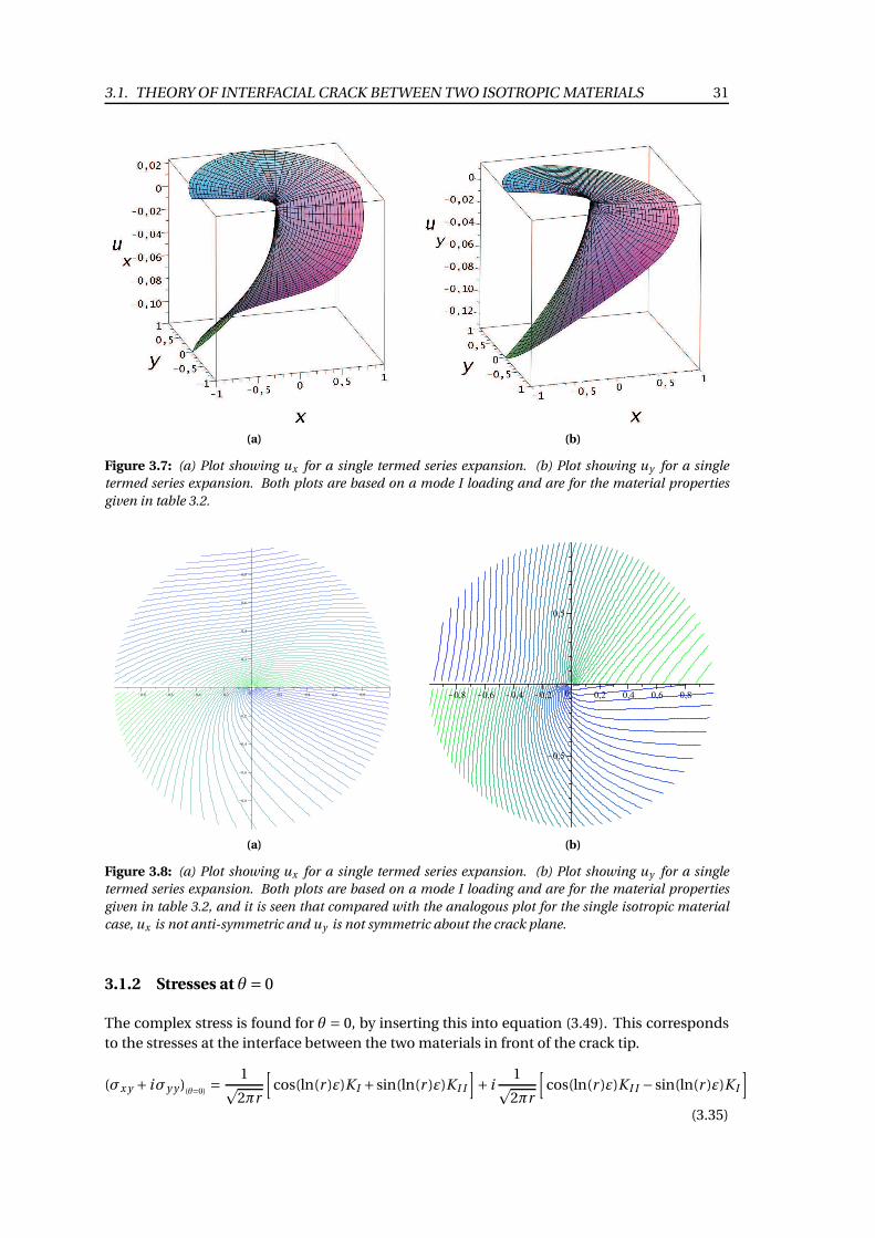
The displacement components ux and uy are plotted in figure 3.7 as the real and imaginary
part of equation (3.34) for K = 83.3+i 76.3 and the material properties given in table 3.2, and as
contourplots in figure 3.8. These contourplots are composed by a separate plot for the upper
and lower material, hence the continuity of the displacements in front of the crack tip (to the
right) is not clear, but the asymmetry is clearly illustrated.
3.1. THEORY OF INTERFACIAL CRACK BETWEEN TWO ISOTROPIC MATERIALS 31
(a) (b)
Figure 3.7: (a) Plot showing ux for a single termed series expansion. (b) Plot showing uy for a single
termed series expansion. Both plots are based on a mode I loading and are for the material properties
given in table 3.2.
(a) (b)
Figure 3.8: (a) Plot showing ux for a single termed series expansion. (b) Plot showing uy for a single
termed series expansion. Both plots are based on a mode I loading and are for the material properties
given in table 3.2, and it is seen that compared with the analogous plot for the single isotropic material
case, ux is not anti-symmetric and uy is not symmetric about the crack plane.
3.1.2 Stresses at θ = 0
The complex stress is found for θ = 0, by inserting this into equation (3.49). This corresponds
to the stresses at the interface between the two materials in front of the crack tip.
(σx y + iσy y )(θ=0)
=1
p2πr
[
cos(ln(r )ε)K I +sin(ln(r )ε)K I I
]
+ i1
p2πr
[
cos(ln(r )ε)K I I −sin(ln(r )ε)K I
]
(3.35)
32 CHAPTER 3. INTERFACE CRACK BETWEEN TWO ISOTROPIC MATERIALS
3.1.3 Displacements at θ =±π
The complex displacement is found for θ = π and θ =−π, which corresponds to the displace-
ment of the crack face for the two materials. For θ = π the eigenfunctions of the displacement
of material 1 is given as:
u(λk ) j=1 =K r λk
p2π
· r iε ·(
1+β)
(i sin(πε))e−πεκ1 +(
1−β)
(i sin(πλk )) eπε
4(λk + iε)µ1(3.36)
For θ =−π the eigenfunctions for the displacement of material 2 are expressed as:
u(λk ) j=2 =K r λk
p2π
· r iε ·(
1−β)
(i sin(−πε))eπεκ2 +(
1+β)
(i sin(−πλk ))e−πε
4(λk + iε)µ2(3.37)
In practice it only makes sense to measure the relative displacement between the crack faces in
the numeric simulation. Hence, the relative displacement is derived for the relative displace-
ment in the x-direction and y-direction, δx and δy , respectively and are given as:
δx = ux, j=1 −ux, j=2
δy = uy, j=1−uy, j=2
}
⇔ (3.38)
δx + i ·δy =(
ux + i uy
)
j=1−
(
ux + i uy
)
j=2(3.39)
In order to obtain the relative complex displacement without K being conjugated as in
equation (3.36) and (3.37) the relative complex displacement is written as:
δy + i ·δx = i (δx + iδy ) (3.40)
= i ((
ux + i uy
)
j=1−
(
ux + i uy
)
j=2) (3.41)
(3.42)
This implies that the eigenfunctions describing the relative complex displacement ∆(λk )
are given as:
∆(λk ) =K r λk r−iε
p2π
(
−i (−1)λk
)
κ1+1µ1
+ κ2+1µ2
4(λk − iε)cosh(πε)(3.43)
The factor(
−i (−1)λk)
implies that the sign of the eigenfunctions change for every λk in the
following way:
λk12
32
52
72
...
−i (−1)λk 1 -1 1 -1 ...
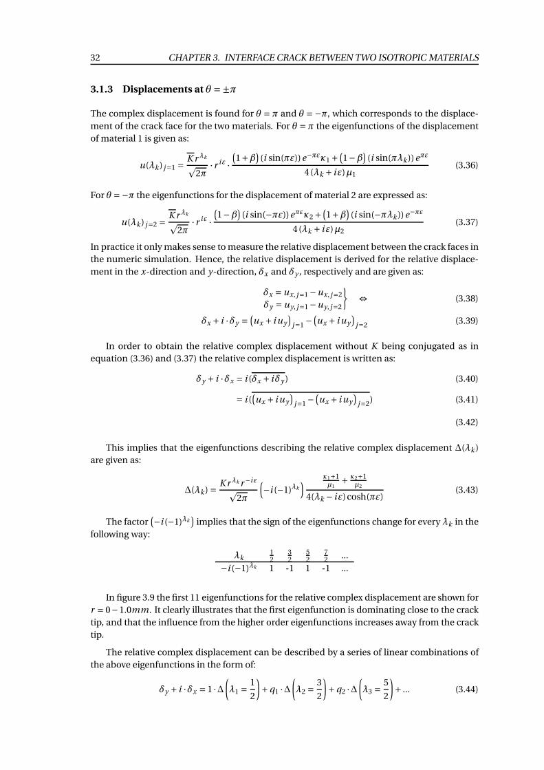
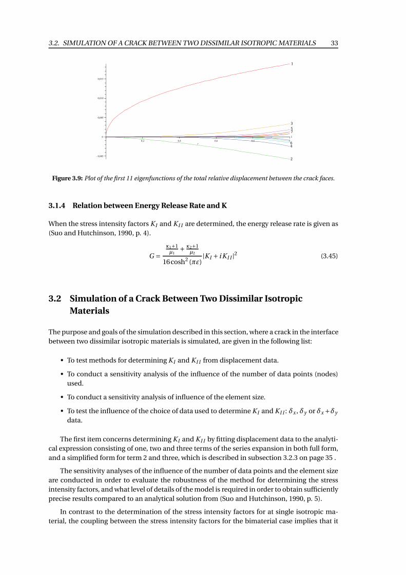
In figure 3.9 the first 11 eigenfunctions for the relative complex displacement are shown for
r = 0−1.0mm. It clearly illustrates that the first eigenfunction is dominating close to the crack
tip, and that the influence from the higher order eigenfunctions increases away from the crack
tip.
The relative complex displacement can be described by a series of linear combinations of
the above eigenfunctions in the form of:
δy + i ·δx = 1 ·∆(
λ1 =1
2
)
+q1 ·∆(
λ2 =3
2
)
+q2 ·∆(
λ3 =5
2
)
+ ... (3.44)
3.2. SIMULATION OF A CRACK BETWEEN TWO DISSIMILAR ISOTROPIC MATERIALS 33
1
2
3
4
5
6
7
...
Figure 3.9: Plot of the first 11 eigenfunctions of the total relative displacement between the crack faces.
3.1.4 Relation between Energy Release Rate and K
When the stress intensity factors K I and K I I are determined, the energy release rate is given as
(Suo and Hutchinson, 1990, p. 4).
G =κ1+1µ1
+ κ2+1µ2
16cosh2 (πε)|K I + i K I I |2 (3.45)
3.2 Simulation of a Crack Between Two Dissimilar Isotropic
Materials
The purpose and goals of the simulation described in this section, where a crack in the interface
between two dissimilar isotropic materials is simulated, are given in the following list:
• To test methods for determining K I and K I I from displacement data.
• To conduct a sensitivity analysis of the influence of the number of data points (nodes)
used.
• To conduct a sensitivity analysis of influence of the element size.
• To test the influence of the choice of data used to determine K I and K I I : δx , δy or δx +δy
data.
The first item concerns determining K I and K I I by fitting displacement data to the analyti-
cal expression consisting of one, two and three terms of the series expansion in both full form,
and a simplified form for term 2 and three, which is described in subsection 3.2.3 on page 35 .
The sensitivity analyses of the influence of the number of data points and the element size
are conducted in order to evaluate the robustness of the method for determining the stress
intensity factors, and what level of details of the model is required in order to obtain sufficiently
precise results compared to an analytical solution from (Suo and Hutchinson, 1990, p. 5).
In contrast to the determination of the stress intensity factors for at single isotropic ma-
terial, the coupling between the stress intensity factors for the bimaterial case implies that it
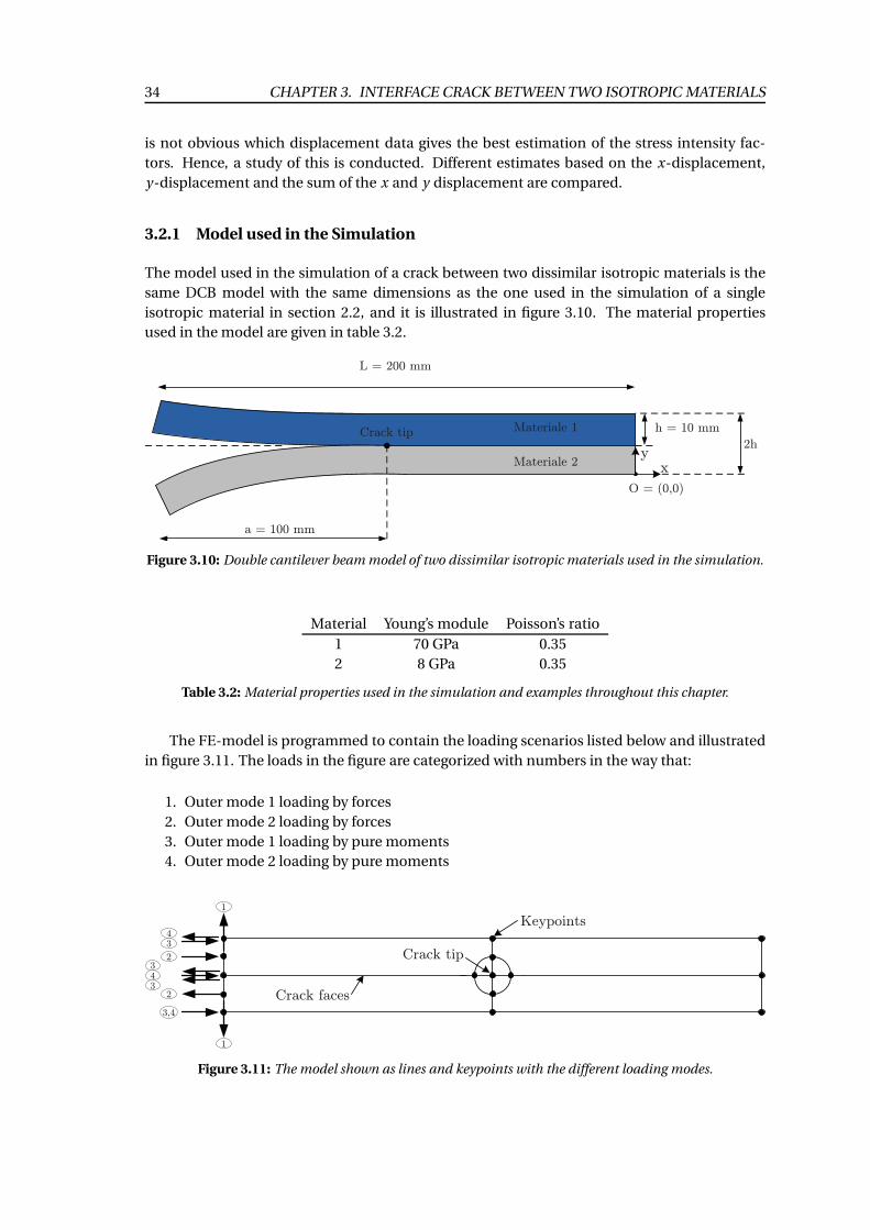
34 CHAPTER 3. INTERFACE CRACK BETWEEN TWO ISOTROPIC MATERIALS
is not obvious which displacement data gives the best estimation of the stress intensity fac-
tors. Hence, a study of this is conducted. Different estimates based on the x-displacement,
y-displacement and the sum of the x and y displacement are compared.
3.2.1 Model used in the Simulation
The model used in the simulation of a crack between two dissimilar isotropic materials is the
same DCB model with the same dimensions as the one used in the simulation of a single
isotropic material in section 2.2, and it is illustrated in figure 3.10. The material properties
used in the model are given in table 3.2.
L = 200 mm
h = 10 mm
a = 100 mm
O = (0,0)
xy
Materiale 1
Materiale 2
2hCrack tip
Figure 3.10: Double cantilever beam model of two dissimilar isotropic materials used in the simulation.
Material Young’s module Poisson’s ratio
1 70 GPa 0.35
2 8 GPa 0.35
Table 3.2: Material properties used in the simulation and examples throughout this chapter.
The FE-model is programmed to contain the loading scenarios listed below and illustrated
in figure 3.11. The loads in the figure are categorized with numbers in the way that:
1. Outer mode 1 loading by forces
2. Outer mode 2 loading by forces
3. Outer mode 1 loading by pure moments
4. Outer mode 2 loading by pure moments
Keypoints
2
2
3,4
Crack tip
Crack faces
34
1
1
343
Figure 3.11: The model shown as lines and keypoints with the different loading modes.
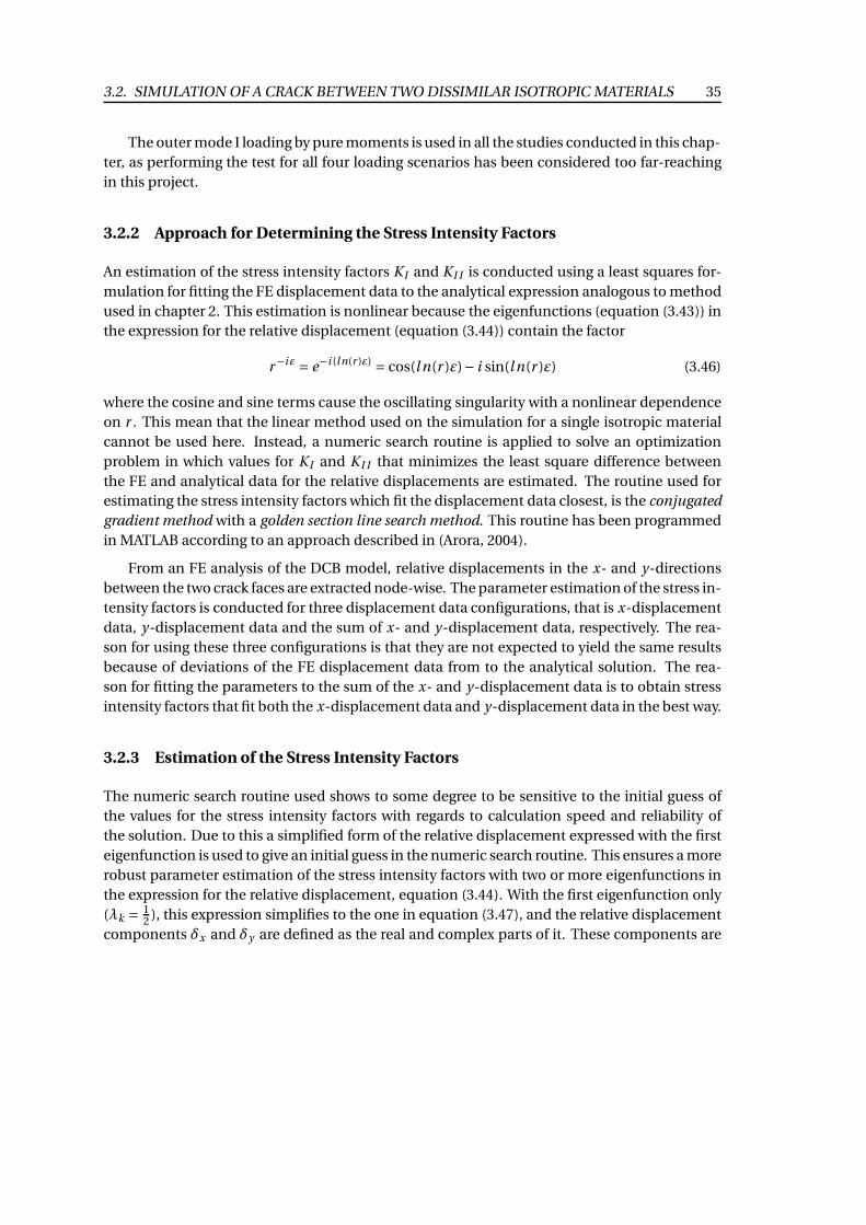
3.2. SIMULATION OF A CRACK BETWEEN TWO DISSIMILAR ISOTROPIC MATERIALS 35
The outer mode I loading by pure moments is used in all the studies conducted in this chap-
ter, as performing the test for all four loading scenarios has been considered too far-reaching
in this project.
3.2.2 Approach for Determining the Stress Intensity Factors
An estimation of the stress intensity factors K I and K I I is conducted using a least squares for-
mulation for fitting the FE displacement data to the analytical expression analogous to method
used in chapter 2. This estimation is nonlinear because the eigenfunctions (equation (3.43)) in
the expression for the relative displacement (equation (3.44)) contain the factor
r−iε = e−i (ln(r )ε) = cos(l n(r )ε)− i sin(l n(r )ε) (3.46)
where the cosine and sine terms cause the oscillating singularity with a nonlinear dependence
on r . This mean that the linear method used on the simulation for a single isotropic material
cannot be used here. Instead, a numeric search routine is applied to solve an optimization
problem in which values for K I and K I I that minimizes the least square difference between
the FE and analytical data for the relative displacements are estimated. The routine used for
estimating the stress intensity factors which fit the displacement data closest, is the conjugated
gradient method with a golden section line search method. This routine has been programmed
in MATLAB according to an approach described in (Arora, 2004).
From an FE analysis of the DCB model, relative displacements in the x- and y-directions
between the two crack faces are extracted node-wise. The parameter estimation of the stress in-
tensity factors is conducted for three displacement data configurations, that is x-displacement
data, y-displacement data and the sum of x- and y-displacement data, respectively. The rea-
son for using these three configurations is that they are not expected to yield the same results
because of deviations of the FE displacement data from to the analytical solution. The rea-
son for fitting the parameters to the sum of the x- and y-displacement data is to obtain stress
intensity factors that fit both the x-displacement data and y-displacement data in the best way.
3.2.3 Estimation of the Stress Intensity Factors
The numeric search routine used shows to some degree to be sensitive to the initial guess of
the values for the stress intensity factors with regards to calculation speed and reliability of
the solution. Due to this a simplified form of the relative displacement expressed with the first
eigenfunction is used to give an initial guess in the numeric search routine. This ensures a more
robust parameter estimation of the stress intensity factors with two or more eigenfunctions in
the expression for the relative displacement, equation (3.44). With the first eigenfunction only
(λk = 12 ), this expression simplifies to the one in equation (3.47), and the relative displacement
components δx and δy are defined as the real and complex parts of it. These components are
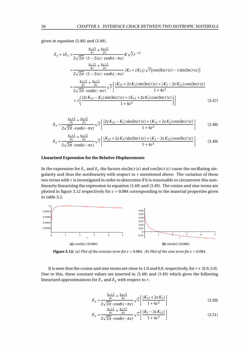
36 CHAPTER 3. INTERFACE CRACK BETWEEN TWO ISOTROPIC MATERIALS
given in equation (3.48) and (3.49).
δy + iδx =κ1+1µ1
+ κ2+1µ2
2p
2π · (1−2iε) ·cosh(−πε)Kp
r r−iε
=κ1+1µ1
+ κ2+1µ2
2p
2π · (1−2iε) ·cosh(−πε)(K I + i K I I )
pr(
cos(ln(r )ε)− i sin(ln(r )ε))
=κ1+1µ1
+ κ2+1µ2
2p
2π ·cosh(−πε)
pr
[
(K I I +2εK I )sin(ln(r )ε)+ (K I −2εK I I )cos(ln(r )ε)
1+4ε2
+ i
(
(2εK I I −K I )sin(ln(r )ε)+ (K I I +2εK I )cos(ln(r )ε)
1+4ε2
)]
(3.47)
δx =κ1+1µ1
+ κ2+1µ2
2p
2π ·cosh(−πε)
pr
[
(2εK I I −K I )sin(ln(r )ε)+ (K I I +2εK I )cos(ln(r )ε)
1+4ε2
]
(3.48)
δy =κ1+1µ1
+ κ2+1µ2
2p
2π ·cosh(−πε)
pr
[
(K I I +2εK I )sin(ln(r )ε)+ (K I −2εK I I )cos(ln(r )ε)
1+4ε2
]
(3.49)
Linearized Expression for the Relative Displacements
In the expression for δx and δy the factors sin(ln(r )ε) and cos(ln(r )ε) cause the oscillating sin-
gularity and thus the nonlinearity with respect to r mentioned above. The variation of these
two terms with r is investigated in order to determine if it is reasonable to circumvent this non-
linearity linearizing the expression in equation (3.48) and (3.49). The cosine and sine terms are
plotted in figure 3.12 respectively for ε= 0.084 corresponding to the material properties given
in table 3.2.
(a) cos(ln(r )0.084) (b) sin(ln(r )0.084)
Figure 3.12: (a) Plot of the consine term for ε= 0.084. (b) Plot of the sine term for ε= 0.084.
It is seen that the cosine and sine terms are close to 1.0 and 0.0, respectively, for r ∈ [0.0,5.0].
Due to this, these constant values are inserted in (3.48) and (3.49) which gives the following
linearized approximations for δx and δy with respect to r .
δx =κ1+1µ1
+ κ2+1µ2
2p
2π ·cosh(−πε)
pr
[
(K I I +2εK I )
1+4ε2
]
(3.50)
δy =κ1+1µ1
+ κ2+1µ2
2p
2π ·cosh(−πε)
pr
[
(K I −2εK I I )
1+4ε2
]
(3.51)
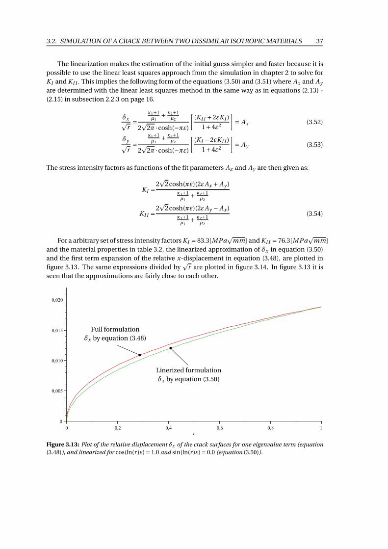
3.2. SIMULATION OF A CRACK BETWEEN TWO DISSIMILAR ISOTROPIC MATERIALS 37
The linearization makes the estimation of the initial guess simpler and faster because it is
possible to use the linear least squares approach from the simulation in chapter 2 to solve for
K I and K I I . This implies the following form of the equations (3.50) and (3.51) where Ax and Ay
are determined with the linear least squares method in the same way as in equations (2.13) -
(2.15) in subsection 2.2.3 on page 16.
δxpr=
κ1+1µ1
+ κ2+1µ2
2p
2π ·cosh(−πε)
[
(K I I +2εK I )
1+4ε2
]
= Ax (3.52)
δypr=
κ1+1µ1
+ κ2+1µ2
2p
2π ·cosh(−πε)
[
(K I −2εK I I )
1+4ε2
]
= Ay (3.53)
The stress intensity factors as functions of the fit parameters Ax and Ay are then given as:
K I =2p
2cosh(πε)(2εAx + Ay )
κ1+1µ1
+ κ2+1µ2
K I I =2p
2cosh(πε)(2εAy − Ax )
κ1+1µ1
+ κ2+1µ2
(3.54)
For a arbitrary set of stress intensity factors K I = 83.3[MPap
mm] and K I I = 76.3[MPap
mm]
and the material properties in table 3.2, the linearized approximation of δx in equation (3.50)
and the first term expansion of the relative x-displacement in equation (3.48), are plotted in
figure 3.13. The same expressions divided byp
r are plotted in figure 3.14. In figure 3.13 it is
seen that the approximations are fairly close to each other.
Full formulation
δx by equation (3.48)
Linerized formulation
δx by equation (3.50)
Figure 3.13: Plot of the relative displacement δx of the crack surfaces for one eigenvalue term (equation
(3.48)), and linearized for cos(ln(r )ε) = 1.0 and sin(ln(r )ε) = 0.0 (equation (3.50)).
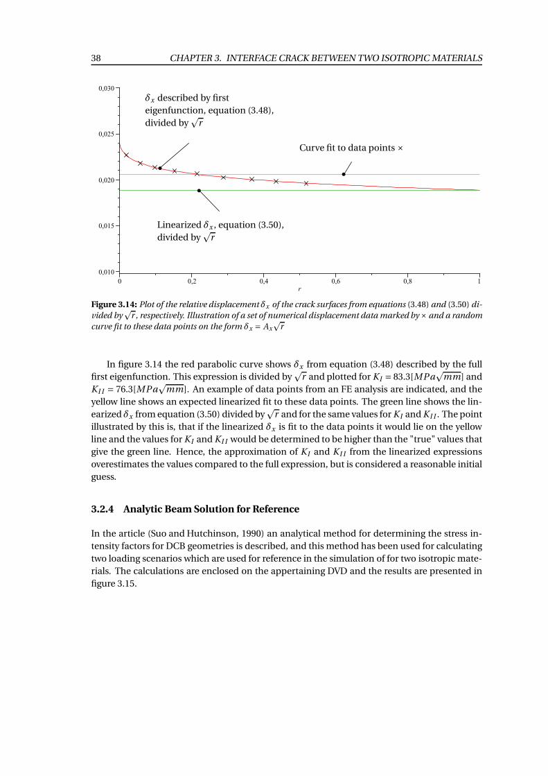
38 CHAPTER 3. INTERFACE CRACK BETWEEN TWO ISOTROPIC MATERIALS
δx described by first
eigenfunction, equation (3.48),
divided byp
r
Linearized δx , equation (3.50),
divided byp
r
Curve fit to data points ×
Figure 3.14: Plot of the relative displacement δx of the crack surfaces from equations (3.48) and (3.50) di-
vided byp
r , respectively. Illustration of a set of numerical displacement data marked by × and a random
curve fit to these data points on the form δx = Axp
r
In figure 3.14 the red parabolic curve shows δx from equation (3.48) described by the full
first eigenfunction. This expression is divided byp
r and plotted for K I = 83.3[MPap
mm] and
K I I = 76.3[MPap
mm]. An example of data points from an FE analysis are indicated, and the
yellow line shows an expected linearized fit to these data points. The green line shows the lin-
earized δx from equation (3.50) divided byp
r and for the same values for K I and K I I . The point
illustrated by this is, that if the linearized δx is fit to the data points it would lie on the yellow
line and the values for K I and K I I would be determined to be higher than the "true" values that
give the green line. Hence, the approximation of K I and K I I from the linearized expressions
overestimates the values compared to the full expression, but is considered a reasonable initial
guess.
3.2.4 Analytic Beam Solution for Reference
In the article (Suo and Hutchinson, 1990) an analytical method for determining the stress in-
tensity factors for DCB geometries is described, and this method has been used for calculating
two loading scenarios which are used for reference in the simulation of for two isotropic mate-
rials. The calculations are enclosed on the appertaining DVD and the results are presented in
figure 3.15.
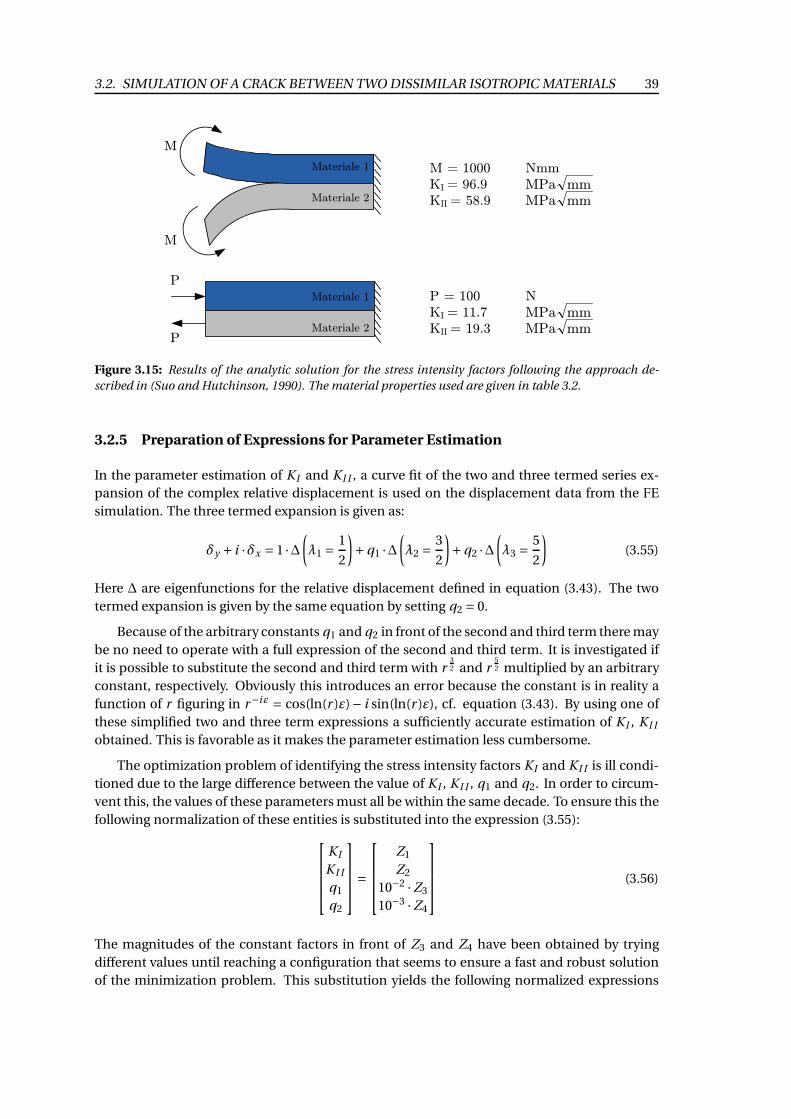
3.2. SIMULATION OF A CRACK BETWEEN TWO DISSIMILAR ISOTROPIC MATERIALS 39
M = 1000 Nmm
KI = 96.9
KII = 58.9
Materiale 1
Materiale 2
M
M
Materiale 1
Materiale 2
P
P
mmMPa
mmMPa
P = 100 N
KI = 11.7
KII = 19.3
mmMPa
mmMPa
Figure 3.15: Results of the analytic solution for the stress intensity factors following the approach de-
scribed in (Suo and Hutchinson, 1990). The material properties used are given in table 3.2.
3.2.5 Preparation of Expressions for Parameter Estimation
In the parameter estimation of K I and K I I , a curve fit of the two and three termed series ex-
pansion of the complex relative displacement is used on the displacement data from the FE
simulation. The three termed expansion is given as:
δy + i ·δx = 1 ·∆(
λ1 =1
2
)
+q1 ·∆(
λ2 =3
2
)
+q2 ·∆(
λ3 =5
2
)
(3.55)
Here ∆ are eigenfunctions for the relative displacement defined in equation (3.43). The two
termed expansion is given by the same equation by setting q2 = 0.
Because of the arbitrary constants q1 and q2 in front of the second and third term there may
be no need to operate with a full expression of the second and third term. It is investigated if
it is possible to substitute the second and third term with r32 and r
52 multiplied by an arbitrary
constant, respectively. Obviously this introduces an error because the constant is in reality a
function of r figuring in r−iε = cos(ln(r )ε)− i sin(ln(r )ε), cf. equation (3.43). By using one of
these simplified two and three term expressions a sufficiently accurate estimation of K I , K I I
obtained. This is favorable as it makes the parameter estimation less cumbersome.
The optimization problem of identifying the stress intensity factors K I and K I I is ill condi-
tioned due to the large difference between the value of K I , K I I , q1 and q2. In order to circum-
vent this, the values of these parameters must all be within the same decade. To ensure this the
following normalization of these entities is substituted into the expression (3.55):
K I
K I I
q1
q2
=
Z1
Z2
10−2 ·Z3
10−3 ·Z4
(3.56)
The magnitudes of the constant factors in front of Z3 and Z4 have been obtained by trying
different values until reaching a configuration that seems to ensure a fast and robust solution
of the minimization problem. This substitution yields the following normalized expressions
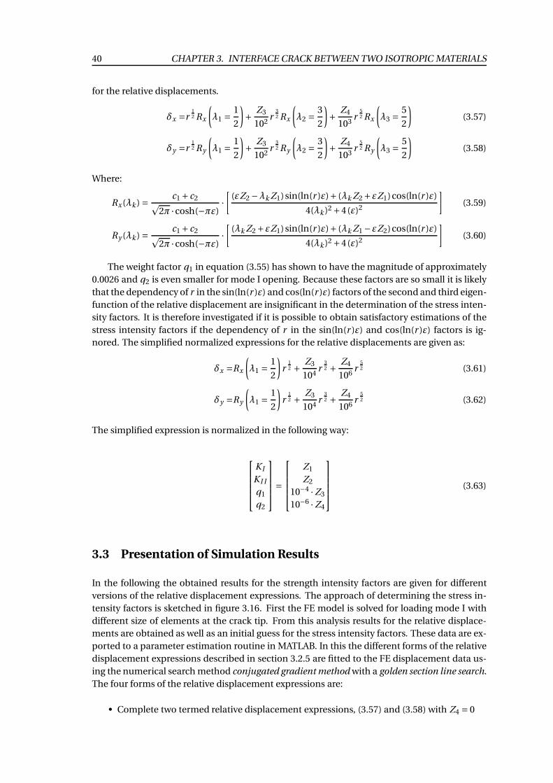
40 CHAPTER 3. INTERFACE CRACK BETWEEN TWO ISOTROPIC MATERIALS
for the relative displacements.
δx =r12 Rx
(
λ1 =1
2
)
+Z3
102r
32 Rx
(
λ2 =3
2
)
+Z4
103r
52 Rx
(
λ3 =5
2
)
(3.57)
δy =r12 Ry
(
λ1 =1
2
)
+Z3
102r
32 Ry
(
λ2 =3
2
)
+Z4
103r
52 Ry
(
λ3 =5
2
)
(3.58)
Where:
Rx (λk ) =c1 +c2p
2π ·cosh(−πε)·[
(εZ2 −λk Z1)sin(ln(r )ε)+ (λk Z2 +εZ1)cos(ln(r )ε)
4(λk )2 +4(ε)2
]
(3.59)
Ry (λk ) =c1 +c2p
2π ·cosh(−πε)·[
(λk Z2 +εZ1)sin(ln(r )ε)+ (λk Z1 −εZ2)cos(ln(r )ε)
4(λk )2 +4(ε)2
]
(3.60)
The weight factor q1 in equation (3.55) has shown to have the magnitude of approximately
0.0026 and q2 is even smaller for mode I opening. Because these factors are so small it is likely
that the dependency of r in the sin(ln(r )ε) and cos(ln(r )ε) factors of the second and third eigen-
function of the relative displacement are insignificant in the determination of the stress inten-
sity factors. It is therefore investigated if it is possible to obtain satisfactory estimations of the
stress intensity factors if the dependency of r in the sin(ln(r )ε) and cos(ln(r )ε) factors is ig-
nored. The simplified normalized expressions for the relative displacements are given as:
δx =Rx
(
λ1 =1
2
)
r12 +
Z3
104r
32 +
Z4
106r
52 (3.61)
δy =Ry
(
λ1 =1
2
)
r12 +
Z3
104r
32 +
Z4
106r
52 (3.62)
The simplified expression is normalized in the following way:
K I
K I I
q1
q2
=
Z1
Z2
10−4 ·Z3
10−6 ·Z4
(3.63)
3.3 Presentation of Simulation Results
In the following the obtained results for the strength intensity factors are given for different
versions of the relative displacement expressions. The approach of determining the stress in-
tensity factors is sketched in figure 3.16. First the FE model is solved for loading mode I with
different size of elements at the crack tip. From this analysis results for the relative displace-
ments are obtained as well as an initial guess for the stress intensity factors. These data are ex-
ported to a parameter estimation routine in MATLAB. In this the different forms of the relative
displacement expressions described in section 3.2.5 are fitted to the FE displacement data us-
ing the numerical search method conjugated gradient method with a golden section line search.
The four forms of the relative displacement expressions are:
• Complete two termed relative displacement expressions, (3.57) and (3.58) with Z4 = 0
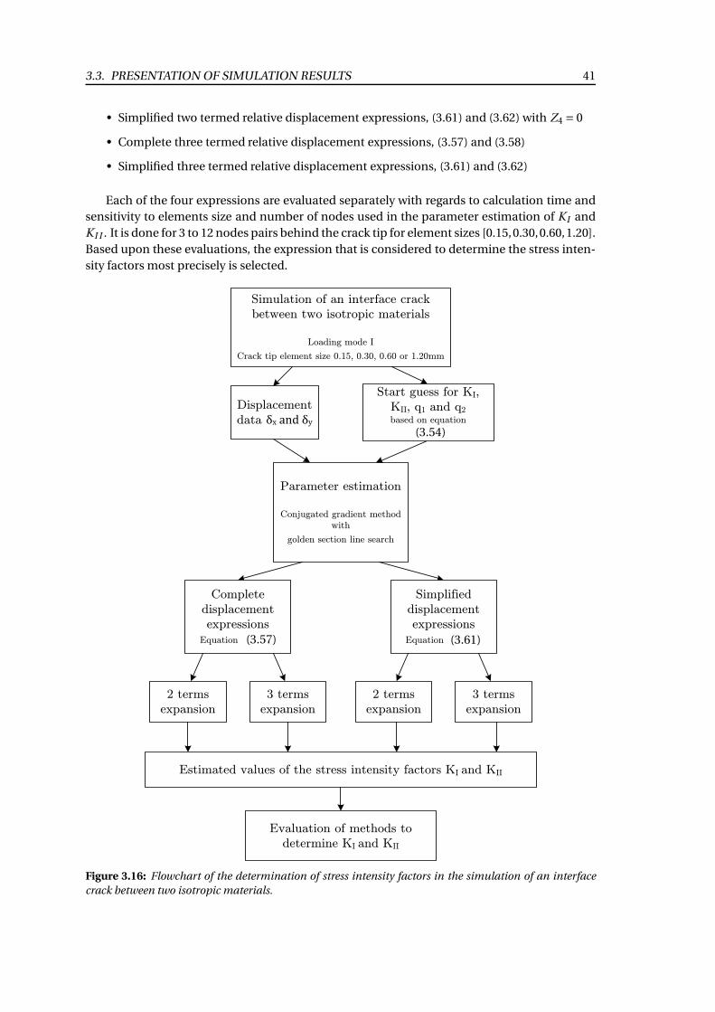
3.3. PRESENTATION OF SIMULATION RESULTS 41
• Simplified two termed relative displacement expressions, (3.61) and (3.62) with Z4 = 0
• Complete three termed relative displacement expressions, (3.57) and (3.58)
• Simplified three termed relative displacement expressions, (3.61) and (3.62)
Each of the four expressions are evaluated separately with regards to calculation time and
sensitivity to elements size and number of nodes used in the parameter estimation of K I and
K I I . It is done for 3 to 12 nodes pairs behind the crack tip for element sizes [0.15,0.30,0.60,1.20].
Based upon these evaluations, the expression that is considered to determine the stress inten-
sity factors most precisely is selected.
Parameter estimation
Conjugated gradient method
with
golden section line search
Simulation of an interface crack
between two isotropic materials
Loading mode I
Crack tip element size 0.15, 0.30, 0.60 or 1.20mm
Displacement
data !
Start guess for KI,
KII, q1 and q2
based on equation
2 terms
expansion
3 terms
expansion
Simplified
displacement
expressions
Equation .
2 terms
expansion
3 terms
expansion
Complete
displacement
expressions
Equation .
Estimated values of the stress intensity factors KI and KII
Evaluation of methods to
determine KI and KII
(3.54)
(3.57) (3.61)
Figure 3.16: Flowchart of the determination of stress intensity factors in the simulation of an interface
crack between two isotropic materials.
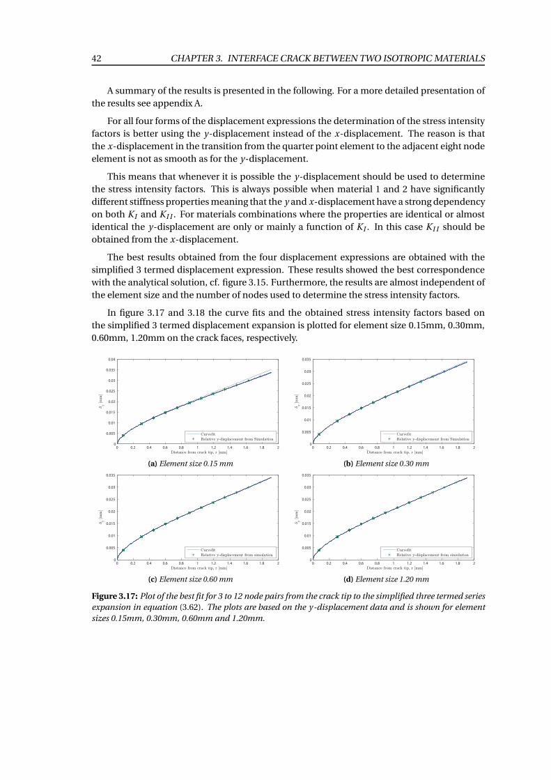
42 CHAPTER 3. INTERFACE CRACK BETWEEN TWO ISOTROPIC MATERIALS
A summary of the results is presented in the following. For a more detailed presentation of
the results see appendix A.
For all four forms of the displacement expressions the determination of the stress intensity
factors is better using the y-displacement instead of the x-displacement. The reason is that
the x-displacement in the transition from the quarter point element to the adjacent eight node
element is not as smooth as for the y-displacement.
This means that whenever it is possible the y-displacement should be used to determine
the stress intensity factors. This is always possible when material 1 and 2 have significantly
different stiffness properties meaning that the y and x-displacement have a strong dependency
on both K I and K I I . For materials combinations where the properties are identical or almost
identical the y-displacement are only or mainly a function of K I . In this case K I I should be
obtained from the x-displacement.
The best results obtained from the four displacement expressions are obtained with the
simplified 3 termed displacement expression. These results showed the best correspondence
with the analytical solution, cf. figure 3.15. Furthermore, the results are almost independent of
the element size and the number of nodes used to determine the stress intensity factors.
In figure 3.17 and 3.18 the curve fits and the obtained stress intensity factors based on
the simplified 3 termed displacement expansion is plotted for element size 0.15mm, 0.30mm,
0.60mm, 1.20mm on the crack faces, respectively.
0 0.2 0.4 0.6 0.8 1 1.2 1.4 1.6 1.8 20
0.005
0.01
0.015
0.02
0.025
0.03
0.035
0.04
Distance from crack tip, r [mm]
δy [
mm
]
CurvefitRelative y-displacement from Simulation
(a) Element size 0.15 mm
0 0.2 0.4 0.6 0.8 1 1.2 1.4 1.6 1.8 20
0.005
0.01
0.015
0.02
0.025
0.03
0.035
Distance from crack tip, r [mm]
δy [
mm
]
CurvefitRelative y-displacement from Simulation
(b) Element size 0.30 mm
0 0.2 0.4 0.6 0.8 1 1.2 1.4 1.6 1.8 20
0.005
0.01
0.015
0.02
0.025
0.03
0.035
Distance from crack tip, r [mm]
δy [
mm
]
CurvefitRelative y-displacement from simulation
(c) Element size 0.60 mm
0 0.2 0.4 0.6 0.8 1 1.2 1.4 1.6 1.8 20
0.005
0.01
0.015
0.02
0.025
0.03
0.035
Distance from crack tip, r [mm]
δy [
mm
]
CurvefitRelative y-displacement from simulation
(d) Element size 1.20 mm
Figure 3.17: Plot of the best fit for 3 to 12 node pairs from the crack tip to the simplified three termed series
expansion in equation (3.62). The plots are based on the y-displacement data and is shown for element
sizes 0.15mm, 0.30mm, 0.60mm and 1.20mm.
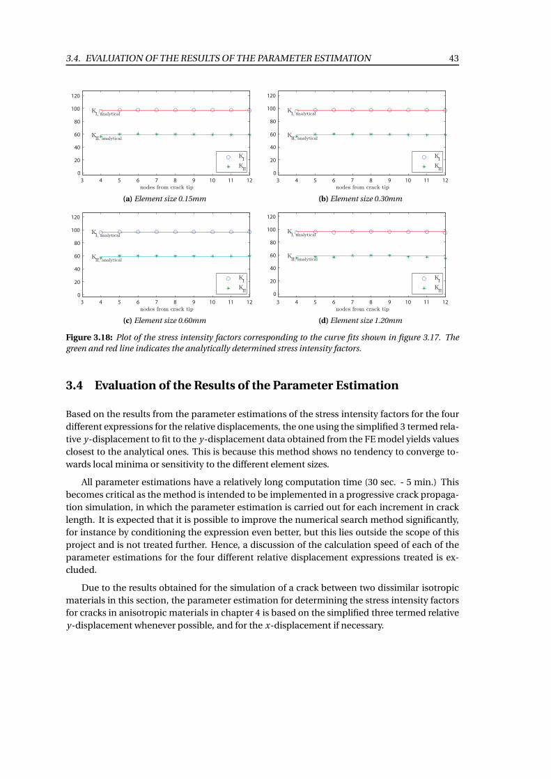
3.4. EVALUATION OF THE RESULTS OF THE PARAMETER ESTIMATION 43
3 4 5 6 7 8 9 10 11 12
0
20
40
60
80
100
120
nodes from crack tip
KI, analytical
KII, analytical
KI
KII
(a) Element size 0.15mm
3 4 5 6 7 8 9 10 11 12
0
20
40
60
80
100
120
nodes from crack tip
KI, analytical
KII, analytical
KI
KII
(b) Element size 0.30mm
3 4 5 6 7 8 9 10 11 12
0
20
40
60
80
100
120
nodes from crack tip
KI, analytical
KII, analytical
KI
KII
(c) Element size 0.60mm
3 4 5 6 7 8 9 10 11 12
0
20
40
60
80
100
120
nodes from crack tip
KI, analytical
KII, analytical
KI
KII
(d) Element size 1.20mm
Figure 3.18: Plot of the stress intensity factors corresponding to the curve fits shown in figure 3.17. The
green and red line indicates the analytically determined stress intensity factors.
3.4 Evaluation of the Results of the Parameter Estimation
Based on the results from the parameter estimations of the stress intensity factors for the four
different expressions for the relative displacements, the one using the simplified 3 termed rela-
tive y-displacement to fit to the y-displacement data obtained from the FE model yields values
closest to the analytical ones. This is because this method shows no tendency to converge to-
wards local minima or sensitivity to the different element sizes.
All parameter estimations have a relatively long computation time (30 sec. - 5 min.) This
becomes critical as the method is intended to be implemented in a progressive crack propaga-
tion simulation, in which the parameter estimation is carried out for each increment in crack
length. It is expected that it is possible to improve the numerical search method significantly,
for instance by conditioning the expression even better, but this lies outside the scope of this
project and is not treated further. Hence, a discussion of the calculation speed of each of the
parameter estimations for the four different relative displacement expressions treated is ex-
cluded.
Due to the results obtained for the simulation of a crack between two dissimilar isotropic
materials in this section, the parameter estimation for determining the stress intensity factors
for cracks in anisotropic materials in chapter 4 is based on the simplified three termed relative
y-displacement whenever possible, and for the x-displacement if necessary.

44 CHAPTER 3. INTERFACE CRACK BETWEEN TWO ISOTROPIC MATERIALS
Summary of Simulation of a Crack Between Two Dissimilar Isotropic
Materials
In this chapter the complete expressions for the stress and displacement field at the crack tip
between two dissimilar isotropic materials is derived. From this the relative displacements
between the two crack faces have been derived. A simulation of a crack in the interface between
the two materials has been conducted in ANSYS with the relative displacements between the
crack faces as output.
Different forms of the equation for the relative displacement have been reformulated into
a minimization problem by use of the least squares method, where the purpose is to determine
the stress intensity factors based on the displacement data from the simulation. Different for-
mulations of the relative displacement together with different element sizes at the crack tip
have been studied. The conclusion is that by using the simplified displacement formulation for
two and three terms, respectively, the problem of determining the stress intensity factors seems
to be convex and satisfactory results are obtained. In addition the simplified three termed dis-
placement formulation makes it possible to use larger element sizes without compromising
the results.
On the other hand if the minimization problem is based on the complete displacement
formulation with two and three terms, respectively, several local minima seem to exist close to
the true values for the stress intensity factors, and this makes it difficult to obtain satisfactory
results.
Chapter
4Interface Crack between TwoDissimilar Anisotropic Materials
In this chapter the theory describing the stress and displacement fields at a crack tip between
two dissimilar anisotropic materials is presented. The procedure for determining the stress in-
tensity factors explained in the previous chapter is extended to the case of a crack between two
anisotropic materials. Furthermore, the R-curve behavior from fiber bridging in fibrous com-
posites is treated and the concept and modeling of fiber bridging is presented and implemented
in a FE model. A test of a double cantilever beam specimen made of orthotropic fiber materials
presented in (Sørensen and Jacobsen, 2009) is briefly described and this specimen is modeled as
a solid FE model. The elastic response of the test specimen is studied and evaluated in compar-
ison to the assumptions in the theory of a crack between dissimilar anisotropic materials and
the assumptions of the article. Finally a simulation of the test specimen with application of the
parameter estimation for determining the energy release rate at the crack tip and bridging across
the crack surfaces is carried out for pure mode I and II, and for mixed mode loading in order to
obtain R-curves for these three scenarios.
4.1 Theory of Interface Crack between Dissimilar Anisotropic
Materials
In continuation of the development of the method used to determine the stress intensity fac-
tors in the simulation of two dissimilar isotropic materials, a theory describing the relative
crack face displacements for a crack in the interface between two dissimilar anisotropic ma-
terials is described in this section. It is presented for anisotropic materials in general, but is in
this chapter only applied to a simulation of two orthotropic fiber composite materials. Both of
these have unidirectional fibers orientated in the x-direction (see figure 4.1) as this is the case
for the test specimen in (Sørensen and Jacobsen, 2009).
The change from considering a crack between two isotropic materials to two anisotropic
materials involves a number of additional challenges. The description of the stress and dis-
placement field around an interface crack between two anisotropic materials involves consti-
tutive laws for the materials which compared to the isotropic material problem are extended
from 2 to 21 independent material parameters. I the general case this implies coupling be-
tween all three crack opening modes for a given external load in opposition to the isotropic
bimaterial problem, where only coupling between modes I and II is present. The is because
45
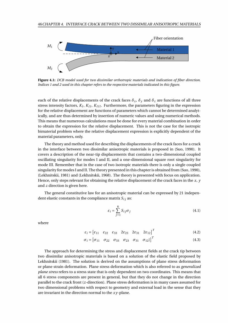
46CHAPTER 4. INTERFACE CRACK BETWEEN TWO DISSIMILAR ANISOTROPIC MATERIALS
xy
z
M1Material 1
Material 2
M2
Fiber orientation
Figure 4.1: DCB model used for two dissimilar orthotropic materials and indication of fiber direction.
Indices 1 and 2 used in this chapter refers to the respective materials indicated in this figure.
each of the relative displacements of the crack faces δx , δy and δz are functions of all three
stress intensity factors, K I , K I I , K I I I . Furthermore, the parameters figuring in the expression
for the relative displacement are functions of parameters which cannot be determined analyt-
ically, and are thus determined by insertion of numeric values and using numerical methods.
This means that numerous calculations must be done for every material combination in order
to obtain the expression for the relative displacement. This is not the case for the isotropic
bimaterial problem where the relative displacement expression is explicitly dependent of the
material parameters, only.
The theory and method used for describing the displacements of the crack faces for a crack
in the interface between two dissimilar anisotropic materials is proposed in (Suo, 1990). It
covers a description of the near-tip displacements that contains a two-dimensional coupled
oscillating singularity for modes I and II, and a one-dimensional square root singularity for
mode III. Remember that in the case of two isotropic materials there is only a single coupled
singularity for modes I and II. The theory presented in this chapter is obtained from (Suo, 1990),
(Lekhnitskii, 1981) and (Lekhnitskii, 1968). The theory is presented with focus on application.
Hence, only steps relevant for obtaining the relative displacement of the crack faces in the x, y
and z direction is given here.
The general constitutive law for an anisotropic material can be expressed by 21 indepen-
dent elastic constants in the compliance matrix Si j as:
εi =6
∑
j=1
Si jσ j (4.1)
where
εi =[
ε11 ε22 ε33 2ε23 2ε31 2ε12
]T(4.2)
σi =[
σ11 σ22 σ33 σ23 σ31 σ12]]T
(4.3)
The approach for determining the stress and displacement fields at the crack tip between
two dissimilar anisotropic materials is based on a solution of the elastic field proposed by
Lekhnitskii (1981). The solution is derived on the assumptions of plane stress deformation
or plane strain deformation. Plane stress deformation which is also referred to as generalized
plane stress refers to a stress state that is only dependent on two coordinates. This means that
all 6 stress components are present in general, but that they do not change in the direction
parallel to the crack front (z-direction). Plane stress deformation is in many cases assumed for
two dimensional problems with respect to geometry and external load in the sense that they
are invariant in the direction normal to the x y-plane.
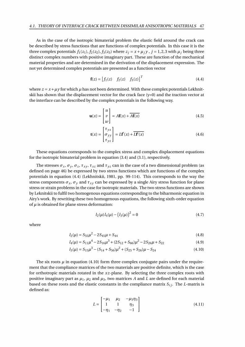
4.1. THEORY OF INTERFACE CRACK BETWEEN DISSIMILAR ANISOTROPIC MATERIALS 47
As in the case of the isotropic bimaterial problem the elastic field around the crack can
be described by stress functions that are functions of complex potentials. In this case it is the
three complex potentials f1(z1), f2(z2), f3(z3) where z j = x +µ j y , j = 1,2,3 with µ j being three
distinct complex numbers with positive imaginary part. These are function of the mechanical
material properties and are determined in the derivation of the displacement expression. The
not yet determined complex potentials are presented as a function vector
f(z)=[
f1(z) f2(z) f3(z)]T
(4.4)
where z = x+µy for which µ has not been determined. With these complex potentials Lekhnit-
skii has shown that the displacement vector for the crack face (y=0) and the traction vector at
the interface can be described by the complex potentials in the following way.
u(x)=
u
v
w
= Af(x)+ Af(x) (4.5)
t(x) =
τy x
σy y
τy z
= Lf′(x)+Lf′(x) (4.6)
These equations corresponds to the complex stress and complex displacement equations
for the isotropic bimaterial problem in equation (3.4) and (3.1), respectively.
The stresses σx , σy , σz , τx y , τxz and τy z can in the case of a two dimensional problem (as
defined on page 46) be expressed by two stress functions which are functions of the complex
potentials in equation (4.4) (Lekhnitskii, 1981, pp. 99-114). This corresponds to the way the
stress components σx , σy and τx y can be expressed by a single Airy stress function for plane
stress or strain problems in the case for isotropic materials. The two stress functions are shown
by Leknitskii to fulfil two homogenous equations corresponding to the biharmonic equation in
Airy’s work. By rewriting these two homogenous equations, the following sixth-order equation
of µ is obtained for plane stress deformation:
l2(µ)l4(µ)−(
l3(µ))2 = 0 (4.7)
where
l2(µ) = S55µ2 −2S45µ+S44 (4.8)
l4(µ) = S11µ4 −2S16µ
3 + (2S12 +S66)µ2 −2S26µ+S22 (4.9)
l3(µ) = S15µ3 − (S14 +S56)µ2 + (S25 +S26)µ−S24 (4.10)
The six roots µ in equation (4.10) form three complex conjugate pairs under the require-
ment that the compliance matrices of the two materials are positive definite, which is the case
for orthotropic materials rotated in the xz-plane. By selecting the three complex roots with
positive imaginary part as µ1, µ2 and µ3, two matrices A and L are defined for each material
based on these roots and the elastic constants in the compliance matrix Si j . The L-matrix is
defined as:
L =
−µ1 µ2 −µ3η3
1 1 η3
−η1 −η2 −1
(4.11)
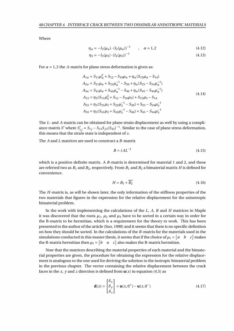
48CHAPTER 4. INTERFACE CRACK BETWEEN TWO DISSIMILAR ANISOTROPIC MATERIALS
Where
ηα =−l3(µα) · (l2(µα))−1 , α= 1,2 (4.12)
η3 =−l3(µ3) · (l4(µ3))−1 (4.13)
For α= 1,2 the A-matrix for plane stress deformation is given as:
A1α = S11µ2α+S12 −S16µα+ηα(S15µα−S14)
A2α = S21µα+S22µ−1α −S26 +ηα(S25−S24µ
−1α )
A3α = S41µα+S42µ−1α −S46 +ηα(S45−S44µ
−1α )
A13 = η3(S11µ23 +S12 −S16µ3)+S15µ3 −S14
A23 = η3(S21µ3 +S22µ−13 −S26)+S25 −S24µ
−13
A33 = η3(S41µ3 +S42µ−13 −S46)+S45 −S44µ
−13
(4.14)
The L- and A-matrix can be obtained for plane strain displacement as well by using a compli-
ance matrix S ′ where S ′i j= Si j −Si 3S j 3(S33)−1. Similar to the case of plane stress deformation,
this means that the strain state is independent of z.
The A and L matrices are used to construct a B-matrix
B = i AL−1 (4.15)
which is a positive definite matrix. A B-matrix is determined for material 1 and 2, and these
are referred two as B1 and B2, respectively. From B1 and B2 a bimaterial matrix H is defined for
convenience.
H = B1 +B2 (4.16)
The H-matrix is, as will be shown later, the only information of the stiffness properties of the
two materials that figures in the expression for the relative displacement for the anisotropic
bimaterial problem.
In the work with implementing the calculations of the L, A, B and H matrices in Maple
it was discovered that the roots µ1, µ2 and µ3 have to be sorted in a certain way in order for
the B-matrix to be hermitian, which is a requirement for the theory to work. This has been
presented to the author of the article (Suo, 1990) and it seems that there is no specific definition
on how they should be sorted. In the calculations of the B-matrix for the materials used in the
simulations conducted in this master thesis, it seems that if the choice of µi =[
a b c]
makes
the B-matrix hermitian then µi =[
b a c]
also makes the B-matrix hermitian.
Now that the matrices describing the material properties of each material and the bimate-
rial properties are given, the procedure for obtaining the expression for the relative displace-
ment is analogous to the one used for deriving the solution to the isotropic bimaterial problem
in the previous chapter. The vector containing the relative displacement between the crack
faces in the x, y and z direction is defined from u(x) in equation (4.5) as
d(x)=
δx
δy
δz
=u(x,0+)−u(x,0−) (4.17)
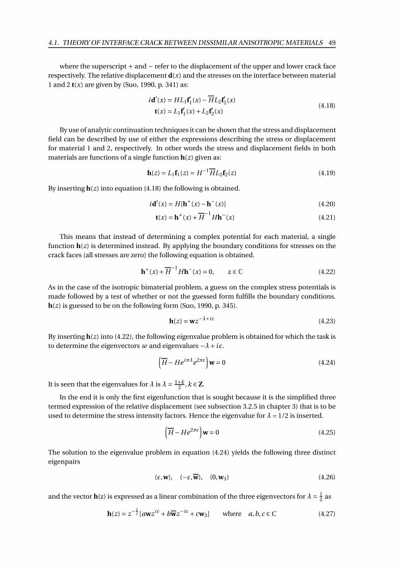
4.1. THEORY OF INTERFACE CRACK BETWEEN DISSIMILAR ANISOTROPIC MATERIALS 49
where the superscript + and − refer to the displacement of the upper and lower crack face
respectively. The relative displacement d(x) and the stresses on the interface between material
1 and 2 t(x) are given by (Suo, 1990, p. 341) as:
i d′(x) = HL1f′1(x)−HL2f′2(x)
t(x) = L1f′1(x)+L2f′2(x)(4.18)
By use of analytic continuation techniques it can be shown that the stress and displacement
field can be described by use of either the expressions describing the stress or displacement
for material 1 and 2, respectively. In other words the stress and displacement fields in both
materials are functions of a single function h(z) given as:
h(z) = L1f1(z) = H−1HL2f2(z) (4.19)
By inserting h(z) into equation (4.18) the following is obtained.
i d′(x) = H [h+(x)−h−(x)] (4.20)
t(x) =h+(x)+H−1
H h−(x) (4.21)
This means that instead of determining a complex potential for each material, a single
function h(z) is determined instead. By applying the boundary conditions for stresses on the
crack faces (all stresses are zero) the following equation is obtained.
h+(x)+H−1
H h−(x) = 0, z ∈ C (4.22)
As in the case of the isotropic bimaterial problem, a guess on the complex stress potentials is
made followed by a test of whether or not the guessed form fulfills the boundary conditions.
h(z) is guessed to be on the following form (Suo, 1990, p. 345).
h(z) = wz−λ+iε (4.23)
By inserting h(z) into (4.22), the following eigenvalue problem is obtained for which the task is
to determine the eigenvectors w and eigenvalues −λ+ iε.
(
H −He iπλe2πε)
w = 0 (4.24)
It is seen that the eigenvalues for λ is λ= 1+k2
,k ∈ Z.
In the end it is only the first eigenfunction that is sought because it is the simplified three
termed expression of the relative displacement (see subsection 3.2.5 in chapter 3) that is to be
used to determine the stress intensity factors. Hence the eigenvalue for λ = 1/2 is inserted.
(
H −He2πε)
w = 0 (4.25)
The solution to the eigenvalue problem in equation (4.24) yields the following three distinct
eigenpairs
(ε,w), (−ε,w), (0,w3) (4.26)
and the vector h(z) is expressed as a linear combination of the three eigenvectors for λ= 12
as
h(z) = z− 12 [awziε+bwz−iε+cw3] where a,b,c ∈C (4.27)
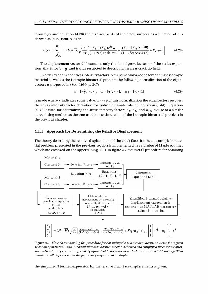
50CHAPTER 4. INTERFACE CRACK BETWEEN TWO DISSIMILAR ANISOTROPIC MATERIALS
From h(z) and equation (4.20) the displacements of the crack surfaces as a function of r is
derived as (Suo, 1990, p. 347):
d(r )=
δx
δy
δz
= (H +H)
√
r
2π
[
(K I + i K I I )r iεw
(1+2iε)cosh(πε)+
(K I − i K I I )r−iεw
(1−2iε)cosh(πε)+K I I I w3
]
(4.28)
The displacement vector d(r) contains only the first eigenvalue term of the series expan-
sion, that is for λ= 12
, and is thus restricted to describing the near crack tip field.
In order to define the stress intensity factors in the same way as done for the single isotropic
material as well as the isotropic bimaterial problem the following normalization of the eigen-
vectors w proposed in (Suo, 1990, p. 347)
w = [−12 i ,∗,∗], w = [ 1
2 i ,∗,∗], w3 = [∗,∗,1] (4.29)
is made where ∗ indicates some value. By use of this normalization the eigenvectors recovers
the stress intensity factor definition for isotropic bimaterials, cf. equation (3.44). Equation
(4.28) is used for determining the stress intensity factors K I , K I I and K I I I by use of a similar
curve fitting method as the one used in the simulation of the isotropic bimaterial problem in
the previous chapter.
4.1.1 Approach for Determining the Relative Displacement
The theory describing the relative displacement of the crack faces for the anisotropic bimate-
rial problem presented in the previous section is implemented in a number of Maple routines
which are enclosed on the appertaining DVD. In figure 4.2 the overall procedure for obtaining
Calculate H
Simplified 3 termed relative
displacement expression is
exported to MATLAB parameter
estimation routine
Solve eigenvalue
problem in equation
and obtain
Obtain relative
displacement by inserting
numerically determined
in equation
Construct Sij Solve for rootsCalculate L1, A1
and B1
Material 1
Construct Sij Solve for rootsCalculate L2, A2
and B2
Material 2Equation (4.7)
(4.25)
w , w3 and ε
H , w , w3 and ε
(4.28)
Equations
(4.7) (4.14) (4.15) Equation (4.16)
µ
µ
δx
δy
δz
= (H +H)√
r2π
[
(KI +i KI I )r iεw(1+2iε)cosh(πε) +
(KI −i KI I )r−iεw(1−2iε)cosh(πε) +K I I I w3
]
+q1
1
1
1
r32 +q2
1
1
1
r52
Figure 4.2: Flow chart showing the procedure for obtaining the relative displacement vector for a given
selection of material 1 and 2. The relative displacement vector is showed as a simplified three term expres-
sion with arbitrary constants q1 and q2 equivalent to the those described in subsection 3.2.5 on page 39 in
chapter 3. All steps shown in the figure are programmed in Maple.
the simplified 3 termed expression for the relative crack face displacements is given.
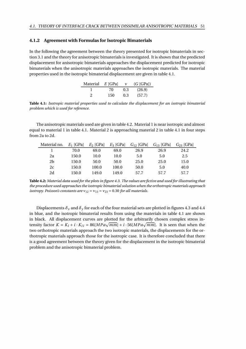
4.1. THEORY OF INTERFACE CRACK BETWEEN DISSIMILAR ANISOTROPIC MATERIALS 51
4.1.2 Agreement with Formulas for Isotropic Bimaterials
In the following the agreement between the theory presented for isotropic bimaterials in sec-
tion 3.1 and the theory for anisotropic bimaterials is investigated. It is shown that the predicted
displacement for anisotropic bimaterials approaches the displacement predicted for isotropic
bimaterials when the anisotropic materials approaches the isotropic materials. The material
properties used in the isotropic bimaterial displacement are given in table 4.1.
Material E [GPa] ν (G [GPa])
1 70 0.3 (26.9)
2 150 0.3 (57.7)
Table 4.1: Isotropic material properties used to calculate the displacement for an isotropic bimaterial
problem which is used for reference.
The anisotropic materials used are given in table 4.2. Material 1 is near isotropic and almost
equal to material 1 in table 4.1. Material 2 is approaching material 2 in table 4.1 in four steps
from 2a to 2d.
Material no. E1 [GPa] E2 [GPa] E3 [GPa] G12 [GPa] G13 [GPa] G23 [GPa]
1 70.0 69.0 69.0 26.9 26.9 24.2
2a 150.0 10.0 10.0 5.0 5.0 2.5
2b 150.0 50.0 50.0 25.0 25.0 15.0
2c 150.0 100.0 100.0 50.0 5.0 40.0
2d 150.0 149.0 149.0 57.7 57.7 57.7
Table 4.2: Material data used for the plots in figure 4.3. The values are fictive and used for illustrating that
the procedure used approaches the isotropic bimaterial solution when the orthotropic materials approach
isotropy. Poisson’s constants are ν12 = ν13 = ν23 = 0.30 for all materials.
Displacements δx and δy for each of the four material sets are plotted in figures 4.3 and 4.4
in blue, and the isotropic bimaterial results from using the materials in table 4.1 are shown
in black. All displacement curves are plotted for the arbitrarily chosen complex stress in-
tensity factor K = K I + i ·K I I = 86[MPap
mm] + i · 56[MPap
mm]. It is seen that when the
two orthotropic materials approach the two isotropic materials, the displacements for the or-
thotropic materials approach those for the isotropic case. It is therefore concluded that there
is a good agreement between the theory given for the displacement in the isotropic bimaterial
problem and the anisotropic bimaterial problem.
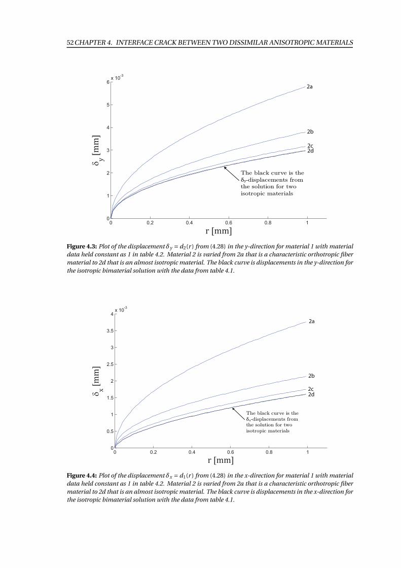
52CHAPTER 4. INTERFACE CRACK BETWEEN TWO DISSIMILAR ANISOTROPIC MATERIALS
0 0.2 0.4 0.6 0.8 10
1
2
3
4
5
6x 10
-3
δ
2a
2b
2c2d
Figure 4.3: Plot of the displacement δy = d2(r ) from (4.28) in the y-direction for material 1 with material
data held constant as 1 in table 4.2. Material 2 is varied from 2a that is a characteristic orthotropic fiber
material to 2d that is an almost isotropic material. The black curve is displacements in the y-direction for
the isotropic bimaterial solution with the data from table 4.1.
0 0.2 0.4 0.6 0.8 10
0.5
1
1.5
2
2.5
3
3.5
4x 10
-3
δ
2a
2b
2c
2d
Figure 4.4: Plot of the displacement δx = d1(r ) from (4.28) in the x-direction for material 1 with material
data held constant as 1 in table 4.2. Material 2 is varied from 2a that is a characteristic orthotropic fiber
material to 2d that is an almost isotropic material. The black curve is displacements in the x-direction for
the isotropic bimaterial solution with the data from table 4.1.
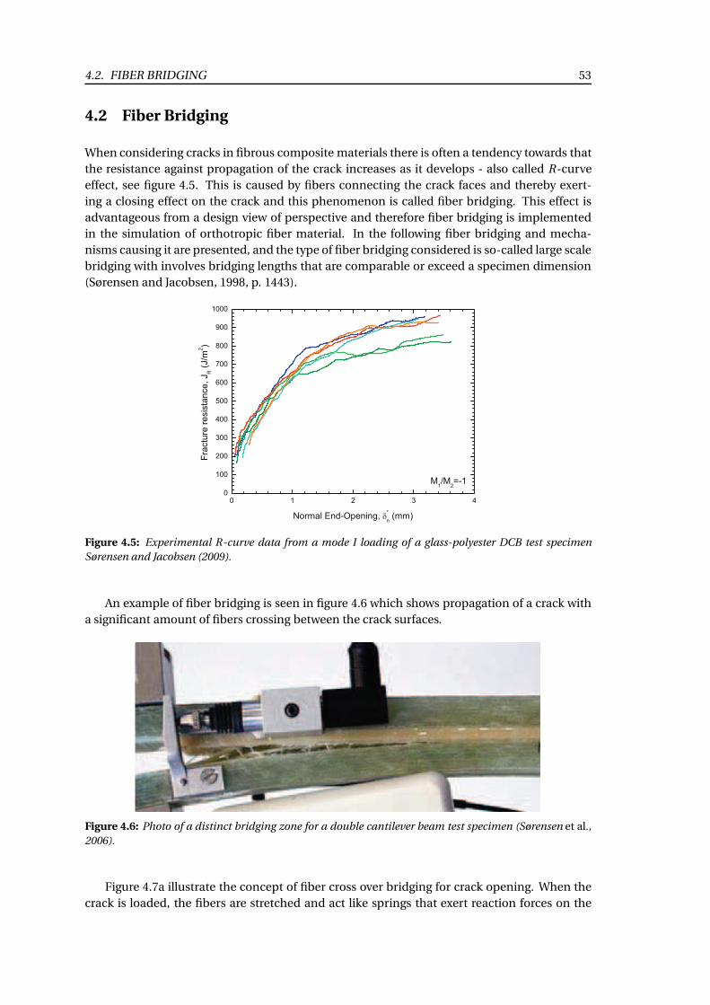
4.2. FIBER BRIDGING 53
4.2 Fiber Bridging
When considering cracks in fibrous composite materials there is often a tendency towards that
the resistance against propagation of the crack increases as it develops - also called R-curve
effect, see figure 4.5. This is caused by fibers connecting the crack faces and thereby exert-
ing a closing effect on the crack and this phenomenon is called fiber bridging. This effect is
advantageous from a design view of perspective and therefore fiber bridging is implemented
in the simulation of orthotropic fiber material. In the following fiber bridging and mecha-
nisms causing it are presented, and the type of fiber bridging considered is so-called large scale
bridging with involves bridging lengths that are comparable or exceed a specimen dimension
(Sørensen and Jacobsen, 1998, p. 1443).
Figure 4.5: Experimental R-curve data from a mode I loading of a glass-polyester DCB test specimen
Sørensen and Jacobsen (2009).
An example of fiber bridging is seen in figure 4.6 which shows propagation of a crack with
a significant amount of fibers crossing between the crack surfaces.
Figure 4.6: Photo of a distinct bridging zone for a double cantilever beam test specimen (Sørensen et al.,
2006).
Figure 4.7a illustrate the concept of fiber cross over bridging for crack opening. When the
crack is loaded, the fibers are stretched and act like springs that exert reaction forces on the
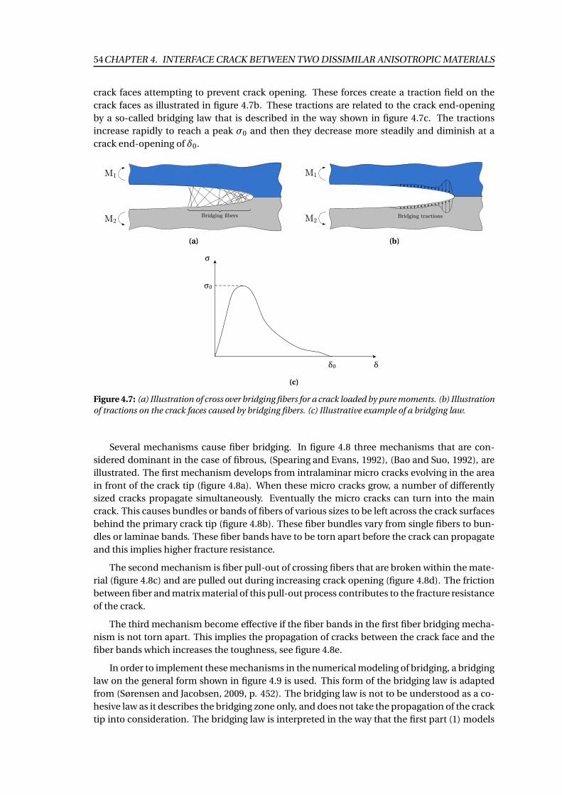
54CHAPTER 4. INTERFACE CRACK BETWEEN TWO DISSIMILAR ANISOTROPIC MATERIALS
crack faces attempting to prevent crack opening. These forces create a traction field on the
crack faces as illustrated in figure 4.7b. These tractions are related to the crack end-opening
by a so-called bridging law that is described in the way shown in figure 4.7c. The tractions
increase rapidly to reach a peak σ0 and then they decrease more steadily and diminish at a
crack end-opening of δ0.
Bridging fibers
M1
M2
(a)
Bridging tractions
M1
M2
(b)
(c)
Figure 4.7: (a) Illustration of cross over bridging fibers for a crack loaded by pure moments. (b) Illustration
of tractions on the crack faces caused by bridging fibers. (c) Illustrative example of a bridging law.
Several mechanisms cause fiber bridging. In figure 4.8 three mechanisms that are con-
sidered dominant in the case of fibrous, (Spearing and Evans, 1992), (Bao and Suo, 1992), are
illustrated. The first mechanism develops from intralaminar micro cracks evolving in the area
in front of the crack tip (figure 4.8a). When these micro cracks grow, a number of differently
sized cracks propagate simultaneously. Eventually the micro cracks can turn into the main
crack. This causes bundles or bands of fibers of various sizes to be left across the crack surfaces
behind the primary crack tip (figure 4.8b). These fiber bundles vary from single fibers to bun-
dles or laminae bands. These fiber bands have to be torn apart before the crack can propagate
and this implies higher fracture resistance.
The second mechanism is fiber pull-out of crossing fibers that are broken within the mate-
rial (figure 4.8c) and are pulled out during increasing crack opening (figure 4.8d). The friction
between fiber and matrix material of this pull-out process contributes to the fracture resistance
of the crack.
The third mechanism become effective if the fiber bands in the first fiber bridging mecha-
nism is not torn apart. This implies the propagation of cracks between the crack face and the
fiber bands which increases the toughness, see figure 4.8e.
In order to implement these mechanisms in the numerical modeling of bridging, a bridging
law on the general form shown in figure 4.9 is used. This form of the bridging law is adapted
from (Sørensen and Jacobsen, 2009, p. 452). The bridging law is not to be understood as a co-
hesive law as it describes the bridging zone only, and does not take the propagation of the crack
tip into consideration. The bridging law is interpreted in the way that the first part (1) models
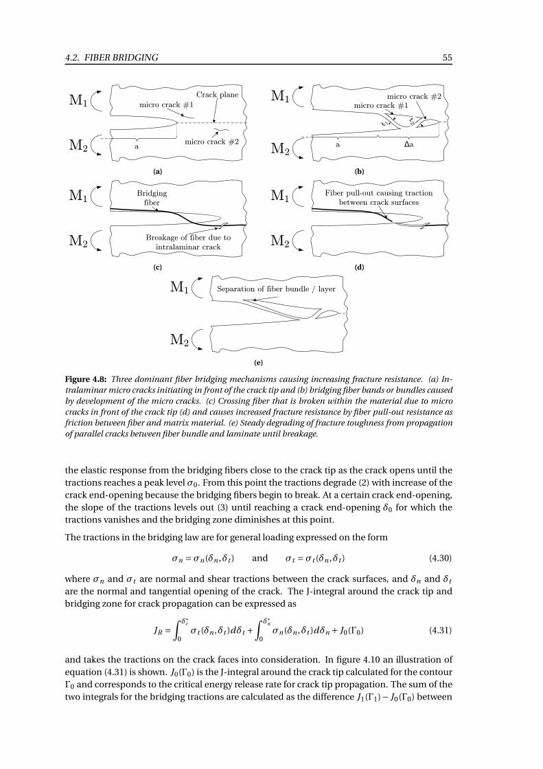
4.2. FIBER BRIDGING 55
Crack plane
micro crack #2a
micro crack #1M1
M2
(a)
micro crack #2
a
micro crack #1
a
t 1
t2
M1
M2
(b)
Breakage of fiber due to intralaminar crack
M1
M2
Bridging fiber
(c)
M1
M2
Fiber pull-out causing traction between crack surfaces
(d)
Separation of fiber bundle / layerM1
M2
(e)
Figure 4.8: Three dominant fiber bridging mechanisms causing increasing fracture resistance. (a) In-
tralaminar micro cracks initiating in front of the crack tip and (b) bridging fiber bands or bundles caused
by development of the micro cracks. (c) Crossing fiber that is broken within the material due to micro
cracks in front of the crack tip (d) and causes increased fracture resistance by fiber pull-out resistance as
friction between fiber and matrix material. (e) Steady degrading of fracture toughness from propagation
of parallel cracks between fiber bundle and laminate until breakage.
the elastic response from the bridging fibers close to the crack tip as the crack opens until the
tractions reaches a peak level σ0. From this point the tractions degrade (2) with increase of the
crack end-opening because the bridging fibers begin to break. At a certain crack end-opening,
the slope of the tractions levels out (3) until reaching a crack end-opening δ0 for which the
tractions vanishes and the bridging zone diminishes at this point.
The tractions in the bridging law are for general loading expressed on the form
σn =σn(δn ,δt ) and σt =σt (δn ,δt ) (4.30)
where σn and σt are normal and shear tractions between the crack surfaces, and δn and δt
are the normal and tangential opening of the crack. The J-integral around the crack tip and
bridging zone for crack propagation can be expressed as
JR =∫δ∗
t
0σt (δn ,δt )dδt +
∫δ∗n
0σn(δn ,δt )dδn + J0(Γ0) (4.31)
and takes the tractions on the crack faces into consideration. In figure 4.10 an illustration of
equation (4.31) is shown. J0(Γ0) is the J-integral around the crack tip calculated for the contour
Γ0 and corresponds to the critical energy release rate for crack tip propagation. The sum of the
two integrals for the bridging tractions are calculated as the difference J1(Γ1)− J0(Γ0) between
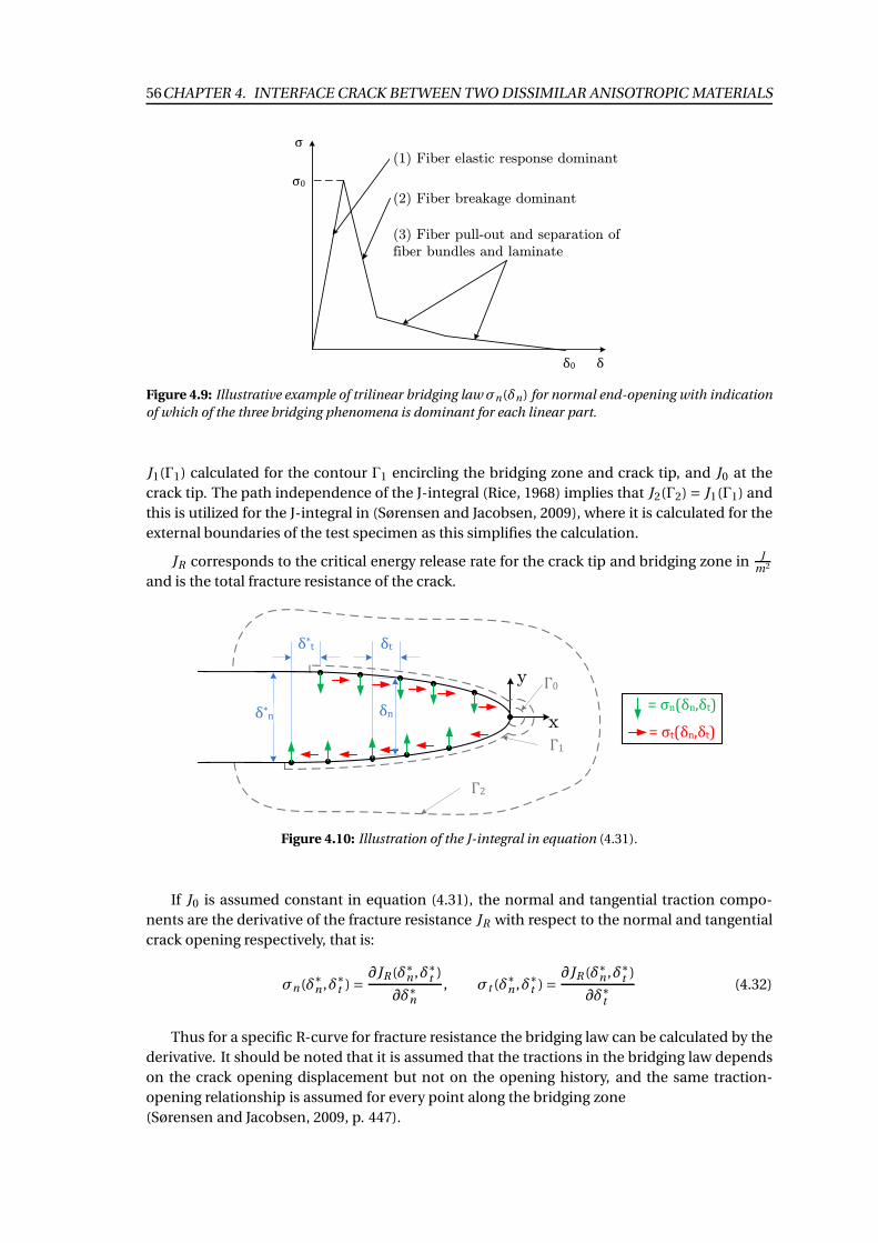
56CHAPTER 4. INTERFACE CRACK BETWEEN TWO DISSIMILAR ANISOTROPIC MATERIALS
(1) Fiber elastic response dominant
(2) Fiber breakage dominant
(3) Fiber pull-out and separation of fiber bundles and laminate
Figure 4.9: Illustrative example of trilinear bridging law σn(δn) for normal end-opening with indication
of which of the three bridging phenomena is dominant for each linear part.
J1(Γ1) calculated for the contour Γ1 encircling the bridging zone and crack tip, and J0 at the
crack tip. The path independence of the J-integral (Rice, 1968) implies that J2(Γ2) = J1(Γ1) and
this is utilized for the J-integral in (Sørensen and Jacobsen, 2009), where it is calculated for the
external boundaries of the test specimen as this simplifies the calculation.
JR corresponds to the critical energy release rate for the crack tip and bridging zone in Jm2
and is the total fracture resistance of the crack.
!"
!#
"
#
$%
$&y
x'()"* "+ #,
'()#* "+ #,
$-
Figure 4.10: Illustration of the J-integral in equation (4.31).
If J0 is assumed constant in equation (4.31), the normal and tangential traction compo-
nents are the derivative of the fracture resistance JR with respect to the normal and tangential
crack opening respectively, that is:
σn(δ∗n ,δ∗t ) =∂JR (δ∗n ,δ∗t )
∂δ∗n, σt (δ∗n ,δ∗t ) =
∂JR (δ∗n ,δ∗t )
∂δ∗t(4.32)
Thus for a specific R-curve for fracture resistance the bridging law can be calculated by the
derivative. It should be noted that it is assumed that the tractions in the bridging law depends
on the crack opening displacement but not on the opening history, and the same traction-
opening relationship is assumed for every point along the bridging zone
(Sørensen and Jacobsen, 2009, p. 447).
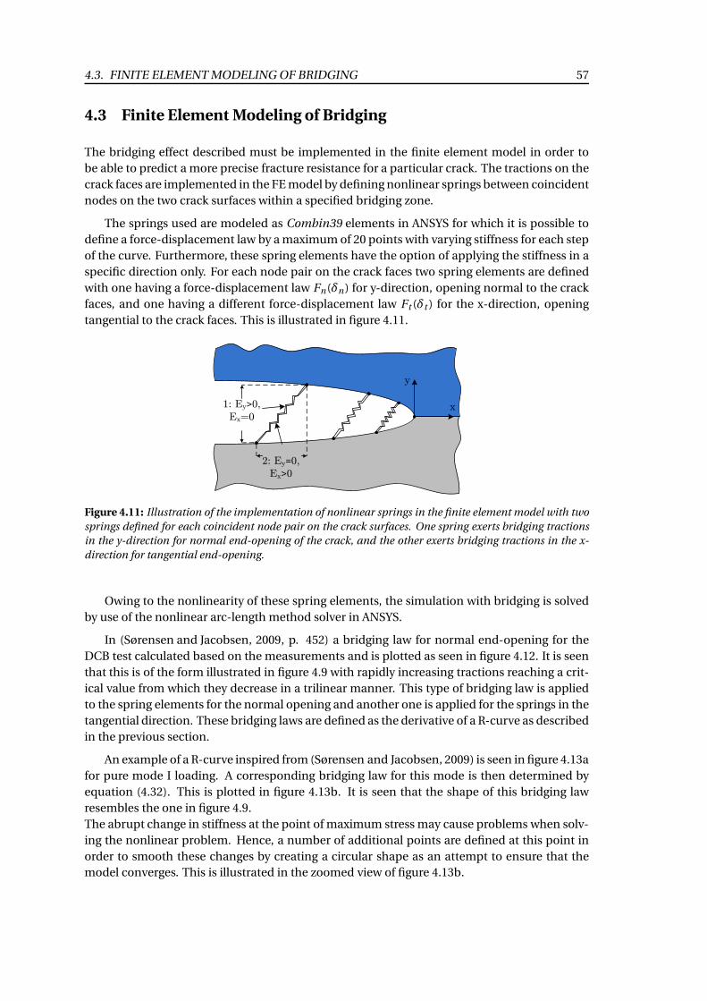
4.3. FINITE ELEMENT MODELING OF BRIDGING 57
4.3 Finite Element Modeling of Bridging
The bridging effect described must be implemented in the finite element model in order to
be able to predict a more precise fracture resistance for a particular crack. The tractions on the
crack faces are implemented in the FE model by defining nonlinear springs between coincident
nodes on the two crack surfaces within a specified bridging zone.
The springs used are modeled as Combin39 elements in ANSYS for which it is possible to
define a force-displacement law by a maximum of 20 points with varying stiffness for each step
of the curve. Furthermore, these spring elements have the option of applying the stiffness in a
specific direction only. For each node pair on the crack faces two spring elements are defined
with one having a force-displacement law Fn(δn) for y-direction, opening normal to the crack
faces, and one having a different force-displacement law Ft (δt ) for the x-direction, opening
tangential to the crack faces. This is illustrated in figure 4.11.
2: Ey 0,
Ex 0
1: Ey 0,
Ex=0
y
x
Figure 4.11: Illustration of the implementation of nonlinear springs in the finite element model with two
springs defined for each coincident node pair on the crack surfaces. One spring exerts bridging tractions
in the y-direction for normal end-opening of the crack, and the other exerts bridging tractions in the x-
direction for tangential end-opening.
Owing to the nonlinearity of these spring elements, the simulation with bridging is solved
by use of the nonlinear arc-length method solver in ANSYS.
In (Sørensen and Jacobsen, 2009, p. 452) a bridging law for normal end-opening for the
DCB test calculated based on the measurements and is plotted as seen in figure 4.12. It is seen
that this is of the form illustrated in figure 4.9 with rapidly increasing tractions reaching a crit-
ical value from which they decrease in a trilinear manner. This type of bridging law is applied
to the spring elements for the normal opening and another one is applied for the springs in the
tangential direction. These bridging laws are defined as the derivative of a R-curve as described
in the previous section.
An example of a R-curve inspired from (Sørensen and Jacobsen, 2009) is seen in figure 4.13a
for pure mode I loading. A corresponding bridging law for this mode is then determined by
equation (4.32). This is plotted in figure 4.13b. It is seen that the shape of this bridging law
resembles the one in figure 4.9.
The abrupt change in stiffness at the point of maximum stress may cause problems when solv-
ing the nonlinear problem. Hence, a number of additional points are defined at this point in
order to smooth these changes by creating a circular shape as an attempt to ensure that the
model converges. This is illustrated in the zoomed view of figure 4.13b.
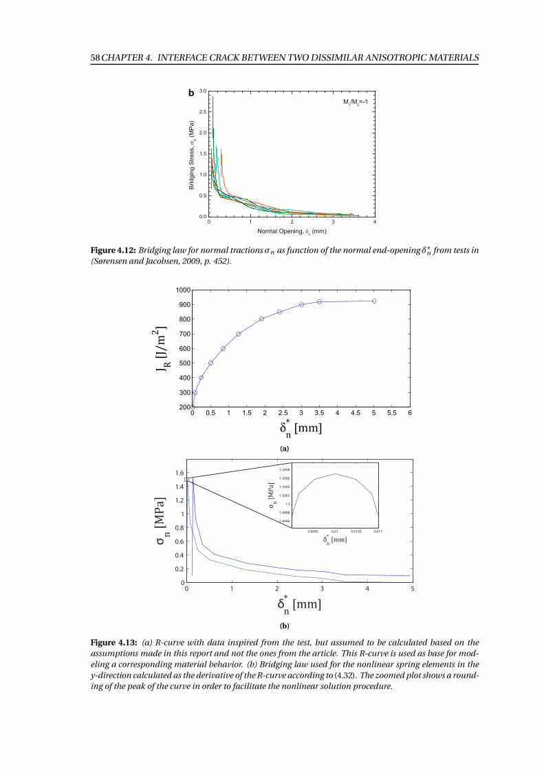
58CHAPTER 4. INTERFACE CRACK BETWEEN TWO DISSIMILAR ANISOTROPIC MATERIALS
b
Figure 4.12: Bridging law for normal tractions σn as function of the normal end-opening δ∗n from tests in
(Sørensen and Jacobsen, 2009, p. 452).
0 0.5 1 1.5 2 2.5 3 3.5 4 4.5 5 5.5 6200
300
400
500
600
700
800
900
1000
δ
!"#$$%
& '"#&($)%
(a)
0 1 2 3 4 50
0.2
0.4
0.6
0.8
1
1.2
1.4
1.6
δ
σ
0.0095 0.01 0.0105 0.011
1.4996
1.4998
1.5
1.5002
1.5004
1.5006
1.5008
δ
σ
(b)
Figure 4.13: (a) R-curve with data inspired from the test, but assumed to be calculated based on the
assumptions made in this report and not the ones from the article. This R-curve is used as base for mod-
eling a corresponding material behavior. (b) Bridging law used for the nonlinear spring elements in the
y-direction calculated as the derivative of the R-curve according to (4.32). The zoomed plot shows a round-
ing of the peak of the curve in order to facilitate the nonlinear solution procedure.
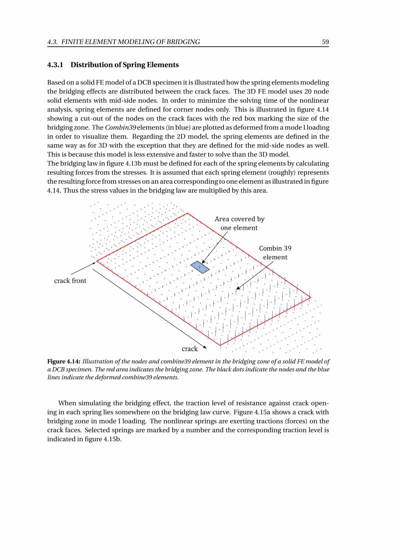
4.3. FINITE ELEMENT MODELING OF BRIDGING 59
4.3.1 Distribution of Spring Elements
Based on a solid FE model of a DCB specimen it is illustrated how the spring elements modeling
the bridging effects are distributed between the crack faces. The 3D FE model uses 20 node
solid elements with mid-side nodes. In order to minimize the solving time of the nonlinear
analysis, spring elements are defined for corner nodes only. This is illustrated in figure 4.14
showing a cut-out of the nodes on the crack faces with the red box marking the size of the
bridging zone. The Combin39 elements (in blue) are plotted as deformed from a mode I loading
in order to visualize them. Regarding the 2D model, the spring elements are defined in the
same way as for 3D with the exception that they are defined for the mid-side nodes as well.
This is because this model is less extensive and faster to solve than the 3D model.
The bridging law in figure 4.13b must be defined for each of the spring elements by calculating
resulting forces from the stresses. It is assumed that each spring element (roughly) represents
the resulting force from stresses on an area corresponding to one element as illustrated in figure
4.14. Thus the stress values in the bridging law are multiplied by this area.
crack front
crack
Figure 4.14: Illustration of the nodes and combine39 element in the bridging zone of a solid FE model of
a DCB specimen. The red area indicates the bridging zone. The black dots indicate the nodes and the blue
lines indicate the deformed combine39 elements.
When simulating the bridging effect, the traction level of resistance against crack open-
ing in each spring lies somewhere on the bridging law curve. Figure 4.15a shows a crack with
bridging zone in mode I loading. The nonlinear springs are exerting tractions (forces) on the
crack faces. Selected springs are marked by a number and the corresponding traction level is
indicated in figure 4.15b.
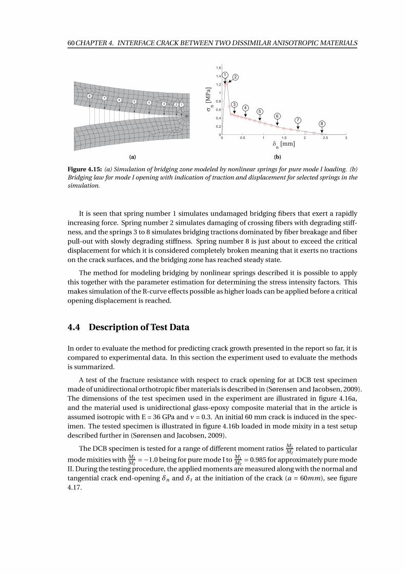
60CHAPTER 4. INTERFACE CRACK BETWEEN TWO DISSIMILAR ANISOTROPIC MATERIALS
1234
56
78
(a)
δ
σ
12
34
5
67
8
(b)
Figure 4.15: (a) Simulation of bridging zone modeled by nonlinear springs for pure mode I loading. (b)
Bridging law for mode I opening with indication of traction and displacement for selected springs in the
simulation.
It is seen that spring number 1 simulates undamaged bridging fibers that exert a rapidly
increasing force. Spring number 2 simulates damaging of crossing fibers with degrading stiff-
ness, and the springs 3 to 8 simulates bridging tractions dominated by fiber breakage and fiber
pull-out with slowly degrading stiffness. Spring number 8 is just about to exceed the critical
displacement for which it is considered completely broken meaning that it exerts no tractions
on the crack surfaces, and the bridging zone has reached steady state.
The method for modeling bridging by nonlinear springs described it is possible to apply
this together with the parameter estimation for determining the stress intensity factors. This
makes simulation of the R-curve effects possible as higher loads can be applied before a critical
opening displacement is reached.
4.4 Description of Test Data
In order to evaluate the method for predicting crack growth presented in the report so far, it is
compared to experimental data. In this section the experiment used to evaluate the methods
is summarized.
A test of the fracture resistance with respect to crack opening for at DCB test specimen
made of unidirectional orthotropic fiber materials is described in (Sørensen and Jacobsen, 2009).
The dimensions of the test specimen used in the experiment are illustrated in figure 4.16a,
and the material used is unidirectional glass-epoxy composite material that in the article is
assumed isotropic with E = 36 GPa and ν = 0.3. An initial 60 mm crack is induced in the spec-
imen. The tested specimen is illustrated in figure 4.16b loaded in mode mixity in a test setup
described further in (Sørensen and Jacobsen, 2009).
The DCB specimen is tested for a range of different moment ratios M1
M2related to particular
mode mixities withM1
M2=−1.0 being for pure mode I to
M1
M2= 0.985 for approximately pure mode
II. During the testing procedure, the applied moments are measured along with the normal and
tangential crack end-opening δn and δt at the initiation of the crack (a = 60mm), see figure
4.17.
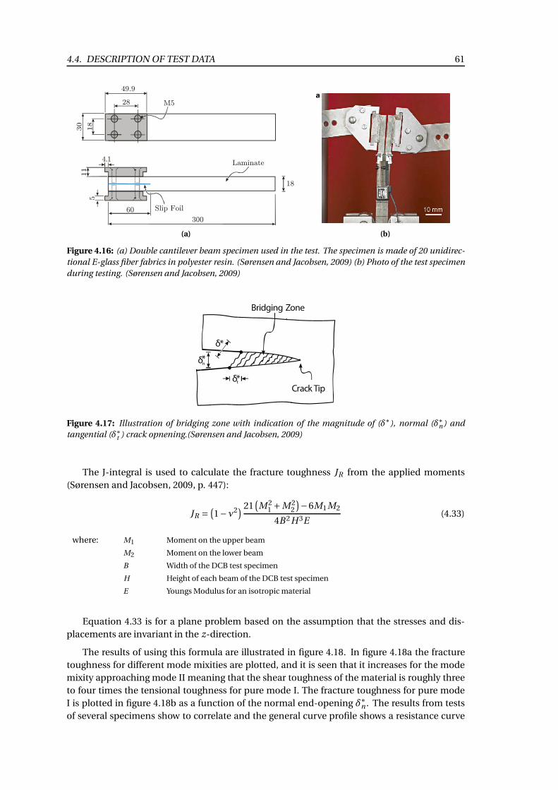
4.4. DESCRIPTION OF TEST DATA 61
300
60
Laminate
Slip Foil
28
49.918
30
M5
11
4.1
5
18
(a)
9
(b)
Figure 4.16: (a) Double cantilever beam specimen used in the test. The specimen is made of 20 unidirec-
tional E-glass fiber fabrics in polyester resin. (Sørensen and Jacobsen, 2009) (b) Photo of the test specimen
during testing. (Sørensen and Jacobsen, 2009)
δn
δ*
*
δt*
Bridging Zone
Crack Tip
Figure 4.17: Illustration of bridging zone with indication of the magnitude of (δ∗), normal (δ∗n) and
tangential (δ∗t ) crack opnening.(Sørensen and Jacobsen, 2009)
The J-integral is used to calculate the fracture toughness JR from the applied moments
(Sørensen and Jacobsen, 2009, p. 447):
JR =(
1−ν2) 21
(
M 21 +M 2
2
)
−6M1M2
4B 2H 3E(4.33)
where: M1 Moment on the upper beam
M2 Moment on the lower beam
B Width of the DCB test specimen
H Height of each beam of the DCB test specimen
E Youngs Modulus for an isotropic material
Equation 4.33 is for a plane problem based on the assumption that the stresses and dis-
placements are invariant in the z-direction.
The results of using this formula are illustrated in figure 4.18. In figure 4.18a the fracture
toughness for different mode mixities are plotted, and it is seen that it increases for the mode
mixity approaching mode II meaning that the shear toughness of the material is roughly three
to four times the tensional toughness for pure mode I. The fracture toughness for pure mode
I is plotted in figure 4.18b as a function of the normal end-opening δ∗n . The results from tests
of several specimens show to correlate and the general curve profile shows a resistance curve
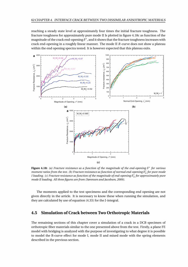
62CHAPTER 4. INTERFACE CRACK BETWEEN TWO DISSIMILAR ANISOTROPIC MATERIALS
reaching a steady state level at approximately four times the initial fracture toughness. The
fracture toughness for approximately pure mode II Is plotted in figure 4.18c as function of the
magnitude of the crack end-openingδ∗, and it shows that the fracture toughness increases with
crack end-opening in a roughly linear manner. The mode II R-curve does not show a plateau
within the end opening spectra tested. It is however expected that this plateau exits.
a
(a) (b)
a
(c)
Figure 4.18: (a) Fracture resistance as a function of the magnitude of the end-opening δ∗ for various
moment ratios from the test. (b) Fracture resistance as function of normal end-opening δ∗n for pure mode
I loading. (c) Fracture resistance as function of the magnitude of end-opening δ∗n for approximately pure
mode II loading. All three figures are from (Sørensen and Jacobsen, 2009).
The moments applied to the test specimens and the corresponding end opening are not
given directly in the article. It is necessary to know these when running the simulation, and
they are calculated by use of equation (4.33) for the J-integral.
4.5 Simulation of Crack between Two Orthotropic Materials
The remaining sections of this chapter cover a simulation of a crack in a DCB specimen of
orthotropic fiber materials similar to the one presented above from the test. Firstly, a plane FE
model with bridging is analyzed with the purpose of investigating to what degree it is possible
to model the R-curve effect for mode I, mode II and mixed mode with the spring elements
described in the previous section.
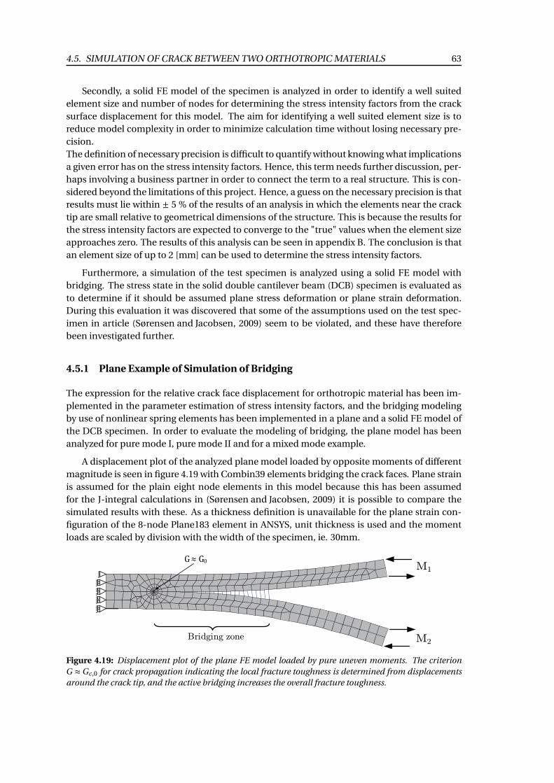
4.5. SIMULATION OF CRACK BETWEEN TWO ORTHOTROPIC MATERIALS 63
Secondly, a solid FE model of the specimen is analyzed in order to identify a well suited
element size and number of nodes for determining the stress intensity factors from the crack
surface displacement for this model. The aim for identifying a well suited element size is to
reduce model complexity in order to minimize calculation time without losing necessary pre-
cision.
The definition of necessary precision is difficult to quantify without knowing what implications
a given error has on the stress intensity factors. Hence, this term needs further discussion, per-
haps involving a business partner in order to connect the term to a real structure. This is con-
sidered beyond the limitations of this project. Hence, a guess on the necessary precision is that
results must lie within ± 5 % of the results of an analysis in which the elements near the crack
tip are small relative to geometrical dimensions of the structure. This is because the results for
the stress intensity factors are expected to converge to the "true" values when the element size
approaches zero. The results of this analysis can be seen in appendix B. The conclusion is that
an element size of up to 2 [mm] can be used to determine the stress intensity factors.
Furthermore, a simulation of the test specimen is analyzed using a solid FE model with
bridging. The stress state in the solid double cantilever beam (DCB) specimen is evaluated as
to determine if it should be assumed plane stress deformation or plane strain deformation.
During this evaluation it was discovered that some of the assumptions used on the test spec-
imen in article (Sørensen and Jacobsen, 2009) seem to be violated, and these have therefore
been investigated further.
4.5.1 Plane Example of Simulation of Bridging
The expression for the relative crack face displacement for orthotropic material has been im-
plemented in the parameter estimation of stress intensity factors, and the bridging modeling
by use of nonlinear spring elements has been implemented in a plane and a solid FE model of
the DCB specimen. In order to evaluate the modeling of bridging, the plane model has been
analyzed for pure mode I, pure mode II and for a mixed mode example.
A displacement plot of the analyzed plane model loaded by opposite moments of different
magnitude is seen in figure 4.19 with Combin39 elements bridging the crack faces. Plane strain
is assumed for the plain eight node elements in this model because this has been assumed
for the J-integral calculations in (Sørensen and Jacobsen, 2009) it is possible to compare the
simulated results with these. As a thickness definition is unavailable for the plane strain con-
figuration of the 8-node Plane183 element in ANSYS, unit thickness is used and the moment
loads are scaled by division with the width of the specimen, ie. 30mm.
G ≈ G0
Bridging zone
M1
M2
Figure 4.19: Displacement plot of the plane FE model loaded by pure uneven moments. The criterion
G ≈ Gc ,0 for crack propagation indicating the local fracture toughness is determined from displacements
around the crack tip, and the active bridging increases the overall fracture toughness.
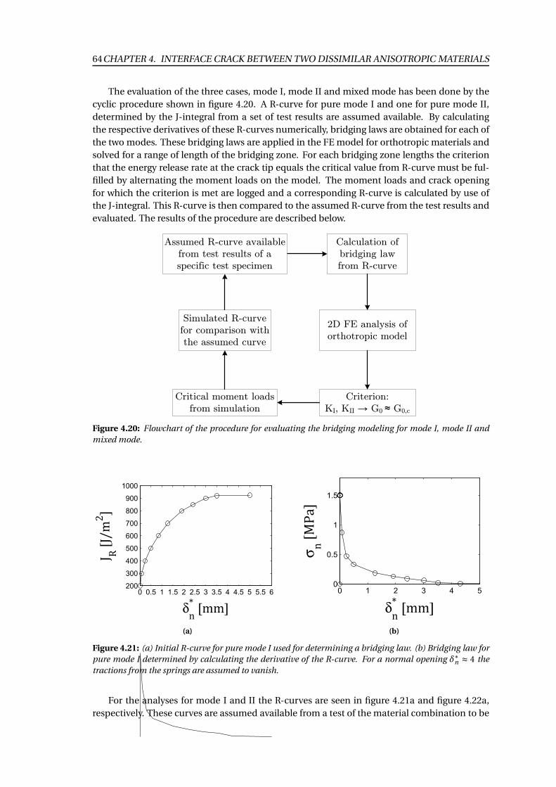
64CHAPTER 4. INTERFACE CRACK BETWEEN TWO DISSIMILAR ANISOTROPIC MATERIALS
The evaluation of the three cases, mode I, mode II and mixed mode has been done by the
cyclic procedure shown in figure 4.20. A R-curve for pure mode I and one for pure mode II,
determined by the J-integral from a set of test results are assumed available. By calculating
the respective derivatives of these R-curves numerically, bridging laws are obtained for each of
the two modes. These bridging laws are applied in the FE model for orthotropic materials and
solved for a range of length of the bridging zone. For each bridging zone lengths the criterion
that the energy release rate at the crack tip equals the critical value from R-curve must be ful-
filled by alternating the moment loads on the model. The moment loads and crack opening
for which the criterion is met are logged and a corresponding R-curve is calculated by use of
the J-integral. This R-curve is then compared to the assumed R-curve from the test results and
evaluated. The results of the procedure are described below.
2D FE analysis of
orthotropic model
Simulated R-curve
for comparison with
the assumed curve
Criterion:
KI, KII G0 ! G0,c
Critical moment loads
from simulation
Assumed R-curve available
from test results of a
specific test specimen
Calculation of
bridging law
from R-curve
Figure 4.20: Flowchart of the procedure for evaluating the bridging modeling for mode I, mode II and
mixed mode.
0 0.5 1 1.5 2 2.5 3 3.5 4 4.5 5 5.5 6200
300
400
500
600
700
800
900
1000
δ
!"#$$%
& '"#&($)%
(a)
"#$$%
0 1 2 3 4 50
0.5
1
1.5
δ
!"#$$%
σ "#*+,%
σ "#*+,%
(b)
Figure 4.21: (a) Initial R-curve for pure mode I used for determining a bridging law. (b) Bridging law for
pure mode I determined by calculating the derivative of the R-curve. For a normal opening δ∗n ≈ 4 the
tractions from the springs are assumed to vanish.
For the analyses for mode I and II the R-curves are seen in figure 4.21a and figure 4.22a,
respectively. These curves are assumed available from a test of the material combination to be
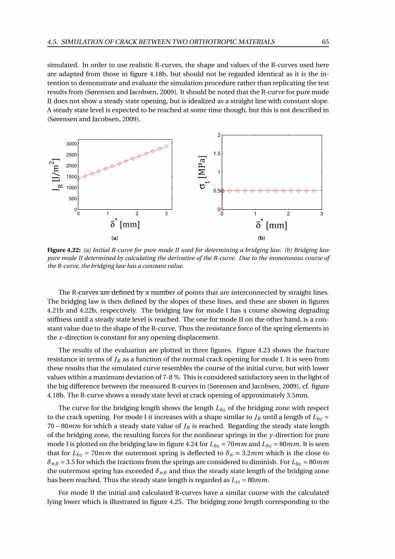
4.5. SIMULATION OF CRACK BETWEEN TWO ORTHOTROPIC MATERIALS 65
simulated. In order to use realistic R-curves, the shape and values of the R-curves used here
are adapted from those in figure 4.18b, but should not be regarded identical as it is the in-
tention to demonstrate and evaluate the simulation procedure rather than replicating the test
results from (Sørensen and Jacobsen, 2009). It should be noted that the R-curve for pure mode
II does not show a steady state opening, but is idealized as a straight line with constant slope.
A steady state level is expected to be reached at some time though, but this is not described in
(Sørensen and Jacobsen, 2009).
0 1 2 30
500
1000
1500
2000
2500
3000
δ !"##$
% &!"%'#
($
(a)
!"##$
0 1 2 30
0.5
1
1.5
2
δ !"##$
σ)!"*
+,$
(b)
Figure 4.22: (a) Initial R-curve for pure mode II used for determining a bridging law. (b) Bridging law
pure mode II determined by calculating the derivative of the R-curve. Due to the monotonous course of
the R-curve, the bridging law has a constant value.
The R-curves are defined by a number of points that are interconnected by straight lines.
The bridging law is then defined by the slopes of these lines, and these are shown in figures
4.21b and 4.22b, respectively. The bridging law for mode I has a course showing degrading
stiffness until a steady state level is reached. The one for mode II on the other hand, is a con-
stant value due to the shape of the R-curve. Thus the resistance force of the spring elements in
the x-direction is constant for any opening displacement.
The results of the evaluation are plotted in three figures. Figure 4.23 shows the fracture
resistance in terms of JR as a function of the normal crack opening for mode I. It is seen from
these results that the simulated curve resembles the course of the initial curve, but with lower
values within a maximum deviation of 7-8 %. This is considered satisfactory seen in the light of
the big difference between the measured R-curves in (Sørensen and Jacobsen, 2009), cf. figure
4.18b. The R-curve shows a steady state level at crack opening of approximately 3.5mm.
The curve for the bridging length shows the length Lbz of the bridging zone with respect
to the crack opening. For mode I it increases with a shape similar to JR until a length of Lbz =70−80mm for which a steady state value of JR is reached. Regarding the steady state length
of the bridging zone, the resulting forces for the nonlinear springs in the y-direction for pure
mode I is plotted on the bridging law in figure 4.24 for Lbz = 70mm and Lbz = 80mm. It is seen
that for Lbz = 70mm the outermost spring is deflected to δn ≈ 3.2mm which is the close to
δn,0 = 3.5 for which the tractions from the springs are considered to diminish. For Lbz = 80mm
the outermost spring has exceeded δn,0 and thus the steady state length of the bridging zone
has been reached. Thus the steady state length is regarded as Lss = 80mm.
For mode II the initial and calculated R-curves have a similar course with the calculated
lying lower which is illustrated in figure 4.25. The bridging zone length corresponding to the

66CHAPTER 4. INTERFACE CRACK BETWEEN TWO DISSIMILAR ANISOTROPIC MATERIALS
0 0.5 1 1.5 2 2.5 3 3.5 4 4.50
200
400
600
800
1000
!"# $
%&'
δ(
)"#%%'
0 0.5 1 1.5 2 2.5 3 3.5 4 4.50
20
40
60
80
100
*+,"#
%%
'
!"-./%"0120
!"3453654017
8.97:9):"51):0;
Figure 4.23: Plot of the initial and calculated values for JR and the bridging zone length Lbz with respect
to the normal crack opening δ∗n for mode I.
0 0.5 1 1.5 2 2.5 3 3.50
0.2
0.4
0.6
0.8
1
1.2
1.4
1.6
δ !"##$
σ !"%&'$
()*+* ,!-'.!/0)!#0+1!2
34)* ,!1-1#1 5!67/0)819:!;<=!>!?@A@!"##$
34)* ,!1-1#1 5!67/0)819:!;<=!>!B@A@!"##$
Figure 4.24: Bridging law for mode I with indication of the resistance forces in the bridging springs in the
y-direction for bridging lengths of Lbz = 70mm and Lbz = 80mm.
tangential opening for this mode are up to approximately three times the steady state length for
mode I for magnitudes of tangential crack opening equal to normal opening. This mode shows
no steady state level, or if it does it is beyond Lbz > 300mm, and this has not been covered in
(Sørensen and Jacobsen, 2009) or in this report.
One example has been calculated for mixed mode loading for which M1
M2= 0.25 meaning
that the moments have the same direction but with M2 being four times M1. This should in-
troduce both mode I and II deformations around the crack tip and thus K I 6= 0 and K I I 6= 0. The
analysis has been made with application of the bridging laws obtained for pure mode I and
mode II respectively in order to evaluate if, or to what degree, this is possible.
Regarding the determination of crack propagation by calculating G0 at the crack tip this
example simplifies in the way that the stress intensity factors K I and K I I decouples because
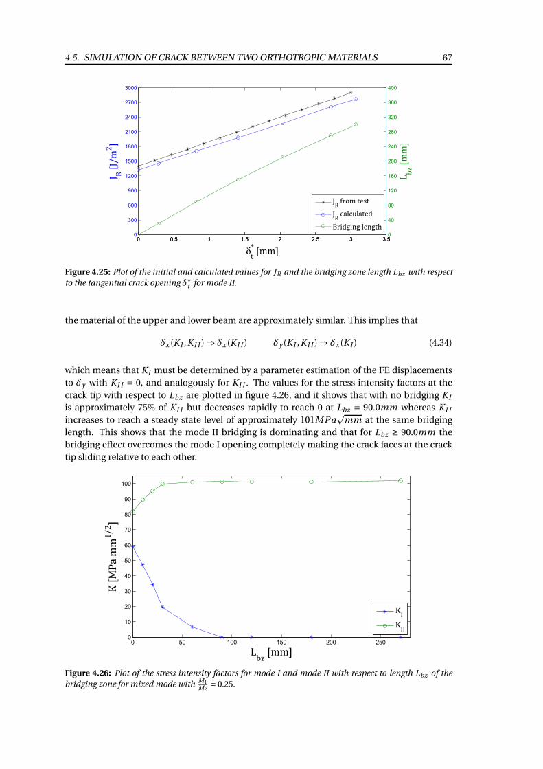
4.5. SIMULATION OF CRACK BETWEEN TWO ORTHOTROPIC MATERIALS 67
0 0.5 1 1.5 2 2.5 3 3.50
300
600
900
1200
1500
1800
2100
2400
2700
3000
!"# $
%&'
δ(
)"#%%'
0 0.5 1 1.5 2 2.5 3 3.50
40
80
120
160
200
240
280
320
360
400
*+,"#
%%
'
!"-./%")01)
!"2342543)06
7.8698:9"40:9);
Figure 4.25: Plot of the initial and calculated values for JR and the bridging zone length Lbz with respect
to the tangential crack opening δ∗t for mode II.
the material of the upper and lower beam are approximately similar. This implies that
δx (K I ,K I I ) ⇒ δx (K I I ) δy (K I ,K I I )⇒ δx (K I ) (4.34)
which means that K I must be determined by a parameter estimation of the FE displacements
to δy with K I I = 0, and analogously for K I I . The values for the stress intensity factors at the
crack tip with respect to Lbz are plotted in figure 4.26, and it shows that with no bridging K I
is approximately 75% of K I I but decreases rapidly to reach 0 at Lbz = 90.0mm whereas K I I
increases to reach a steady state level of approximately 101MPap
mm at the same bridging
length. This shows that the mode II bridging is dominating and that for Lbz ≥ 90.0mm the
bridging effect overcomes the mode I opening completely making the crack faces at the crack
tip sliding relative to each other.
0 50 100 150 200 2500
10
20
30
40
50
60
70
80
90
100
!"#$%!&&'()*
+,-!"&&*
.
..
Figure 4.26: Plot of the stress intensity factors for mode I and mode II with respect to length Lbz of the
bridging zone for mixed mode withM1
M2= 0.25.
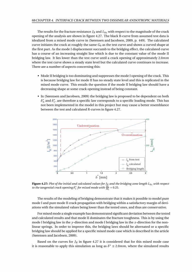
68CHAPTER 4. INTERFACE CRACK BETWEEN TWO DISSIMILAR ANISOTROPIC MATERIALS
The results for the fracture resistance JR and Lbz with respect to the magnitude of the crack
opening of the analysis are shown in figure 4.27. The black R-curve from assumed test data is
idealized from a mixed mode curve in (Sørensen and Jacobsen, 2009, p. 449). The calculated
curve initiates the crack at roughly the same G0 as the test curve and shows a curved shape at
the first part. As the mode I displacement succumb to the bridging effect, the calculated curve
has a course of an increasing straight line which is due to the constant value of the mode II
bridging law. It lies lower than the test curve until a crack opening of approximately 2.0mm
where the test curve shows a steady state level but the calculated curve continues to increase.
There are a number of aspects concerning this:
• Mode II bridging is too dominating and suppresses the mode I opening of the crack. This
is because bridging law for mode II has no steady state level and this is replicated in the
mixed mode curve. This entails the question if the mode II bridging law should have a
decreasing shape at some crack opening instead of being constant.
• In (Sørensen and Jacobsen, 2009) the bridging law is proposed to be dependent on both
δ∗n and δ∗t , are therefore a specific law corresponds to a specific loading mode. This has
not been implemented in the model in this project but may cause a better resemblance
between the test and calculated R-curves in figure 4.27.
δ
Overestimation
Underestimation
Figure 4.27: Plot of the initial and calculated values for JR and the bridging zone length Lbz with respect
to the tangential crack opening δ∗t for mixed mode withM1
M2= 0.25.
The results of the modeling of bridging demonstrate that it makes it possible to model pure
mode I and pure mode II crack propagation with bridging within a satisfactory margin of devi-
ations with the simulated values being lower than the tested ones, and thus are conservative.
For mixed mode a single example has demonstrated significant deviation between the tested
and calculated results and that mode II dominates the fracture toughness. This is by using the
mode I bridging law in the y-direction and mode I bridging law in the x-direction for the non-
linear springs. In order to improve this, the bridging laws should be alternated or a specific
bridging law should be applied for a specific mixed mode case which is described in the article
(Sørensen and Jacobsen, 2009).
Based on the curves for JR in figure 4.27 it is considered that for this mixed mode case
it is reasonable to apply this simulation as long as δ∗ ≤ 2.0mm, where the simulated results
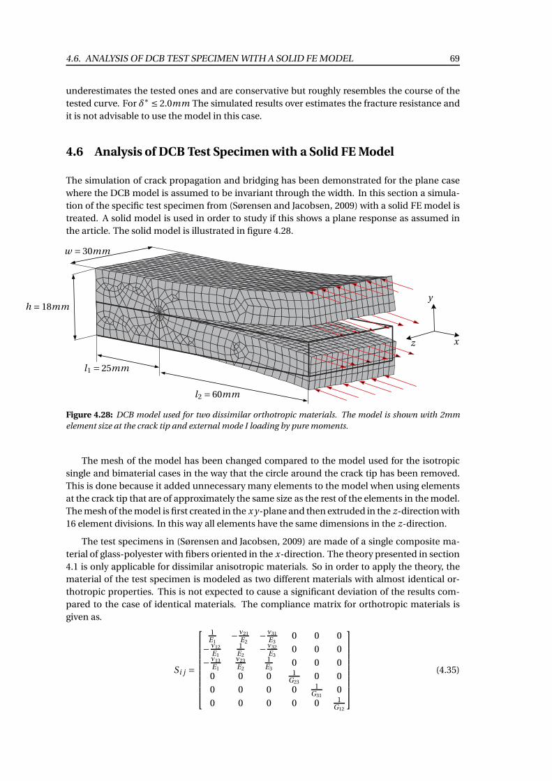
4.6. ANALYSIS OF DCB TEST SPECIMEN WITH A SOLID FE MODEL 69
underestimates the tested ones and are conservative but roughly resembles the course of the
tested curve. For δ∗ ≤ 2.0mm The simulated results over estimates the fracture resistance and
it is not advisable to use the model in this case.
4.6 Analysis of DCB Test Specimen with a Solid FE Model
The simulation of crack propagation and bridging has been demonstrated for the plane case
where the DCB model is assumed to be invariant through the width. In this section a simula-
tion of the specific test specimen from (Sørensen and Jacobsen, 2009) with a solid FE model is
treated. A solid model is used in order to study if this shows a plane response as assumed in
the article. The solid model is illustrated in figure 4.28.
w = 30mm
h = 18mm
l1 = 25mm
l2 = 60mm
x
y
z
Figure 4.28: DCB model used for two dissimilar orthotropic materials. The model is shown with 2mm
element size at the crack tip and external mode I loading by pure moments.
The mesh of the model has been changed compared to the model used for the isotropic
single and bimaterial cases in the way that the circle around the crack tip has been removed.
This is done because it added unnecessary many elements to the model when using elements
at the crack tip that are of approximately the same size as the rest of the elements in the model.
The mesh of the model is first created in the x y-plane and then extruded in the z-direction with
16 element divisions. In this way all elements have the same dimensions in the z-direction.
The test specimens in (Sørensen and Jacobsen, 2009) are made of a single composite ma-
terial of glass-polyester with fibers oriented in the x-direction. The theory presented in section
4.1 is only applicable for dissimilar anisotropic materials. So in order to apply the theory, the
material of the test specimen is modeled as two different materials with almost identical or-
thotropic properties. This is not expected to cause a significant deviation of the results com-
pared to the case of identical materials. The compliance matrix for orthotropic materials is
given as.
Si j =
1E1
−ν21
E2−ν31
E30 0 0
−ν12
E1
1E2
−ν32
E30 0 0
−ν13
E1
ν23
E2
1E3
0 0 0
0 0 0 1G23
0 0
0 0 0 0 1G31
0
0 0 0 0 0 1G12
(4.35)
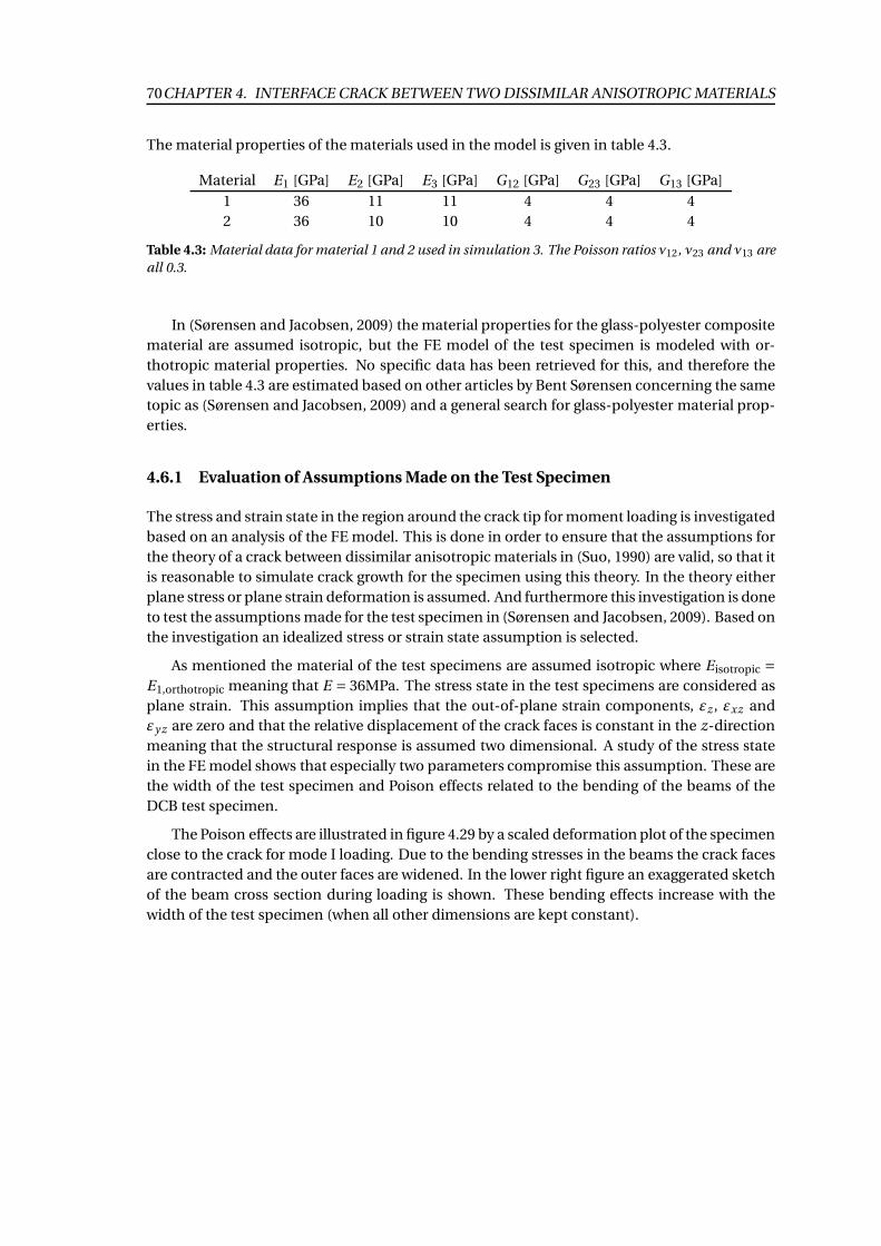
70CHAPTER 4. INTERFACE CRACK BETWEEN TWO DISSIMILAR ANISOTROPIC MATERIALS
The material properties of the materials used in the model is given in table 4.3.
Material E1 [GPa] E2 [GPa] E3 [GPa] G12 [GPa] G23 [GPa] G13 [GPa]
1 36 11 11 4 4 4
2 36 10 10 4 4 4
Table 4.3: Material data for material 1 and 2 used in simulation 3. The Poisson ratios ν12, ν23 and ν13 are
all 0.3.
In (Sørensen and Jacobsen, 2009) the material properties for the glass-polyester composite
material are assumed isotropic, but the FE model of the test specimen is modeled with or-
thotropic material properties. No specific data has been retrieved for this, and therefore the
values in table 4.3 are estimated based on other articles by Bent Sørensen concerning the same
topic as (Sørensen and Jacobsen, 2009) and a general search for glass-polyester material prop-
erties.
4.6.1 Evaluation of Assumptions Made on the Test Specimen
The stress and strain state in the region around the crack tip for moment loading is investigated
based on an analysis of the FE model. This is done in order to ensure that the assumptions for
the theory of a crack between dissimilar anisotropic materials in (Suo, 1990) are valid, so that it
is reasonable to simulate crack growth for the specimen using this theory. In the theory either
plane stress or plane strain deformation is assumed. And furthermore this investigation is done
to test the assumptions made for the test specimen in (Sørensen and Jacobsen, 2009). Based on
the investigation an idealized stress or strain state assumption is selected.
As mentioned the material of the test specimens are assumed isotropic where Eisotropic =E1,orthotropic meaning that E = 36MPa. The stress state in the test specimens are considered as
plane strain. This assumption implies that the out-of-plane strain components, εz , εxz and
εy z are zero and that the relative displacement of the crack faces is constant in the z-direction
meaning that the structural response is assumed two dimensional. A study of the stress state
in the FE model shows that especially two parameters compromise this assumption. These are
the width of the test specimen and Poison effects related to the bending of the beams of the
DCB test specimen.
The Poison effects are illustrated in figure 4.29 by a scaled deformation plot of the specimen
close to the crack for mode I loading. Due to the bending stresses in the beams the crack faces
are contracted and the outer faces are widened. In the lower right figure an exaggerated sketch
of the beam cross section during loading is shown. These bending effects increase with the
width of the test specimen (when all other dimensions are kept constant).
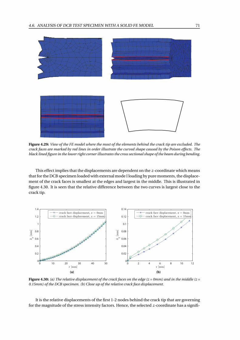
4.6. ANALYSIS OF DCB TEST SPECIMEN WITH A SOLID FE MODEL 71
X
Y
Z
Figure 4.29: View of the FE model where the most of the elements behind the crack tip are excluded. The
crack faces are marked by red lines in order illustrate the curved shape caused by the Poison effects. The
black lined figure in the lower right corner illustrates the cross sectional shape of the beam during bending.
This effect implies that the displacements are dependent on the z-coordinate which means
that for the DCB specimen loaded with external mode I loading by pure moments, the displace-
ment of the crack faces is smallest at the edges and largest in the middle. This is illustrated in
figure 4.30. It is seen that the relative difference between the two curves is largest close to the
crack tip.
0 10 20 30 40 500
0.2
0.4
0.6
0.8
1
1.2
1.4
r [mm]
δy [m
m]
crack face displacement, z = 0mmcrack face displacement, z = 15mm
(a)
0 2 4 6 8 10 120
0.02
0.04
0.06
0.08
0.1
0.12
0.14
r [mm]
δy [m
m]
crack face displacement, z = 0mmcrack face displacement, z = 15mm
(b)
Figure 4.30: (a) The relative displacement of the crack faces on the edge (z = 0mm) and in the middle (z =
0.15mm) of the DCB specimen. (b) Close up of the relative crack face displacement.
It is the relative displacements of the first 1-2 nodes behind the crack tip that are governing
for the magnitude of the stress intensity factors. Hence, the selected z-coordinate has a signifi-
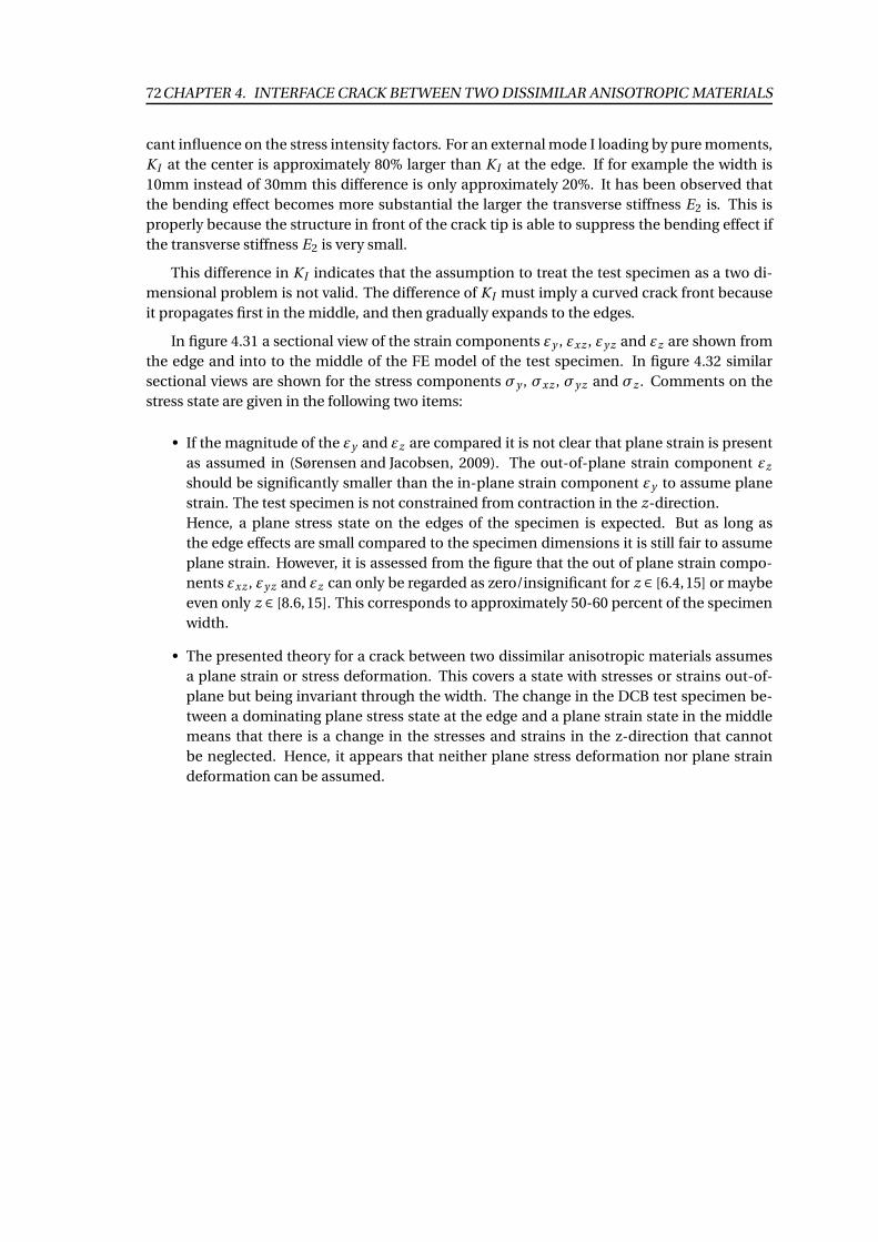
72CHAPTER 4. INTERFACE CRACK BETWEEN TWO DISSIMILAR ANISOTROPIC MATERIALS
cant influence on the stress intensity factors. For an external mode I loading by pure moments,
K I at the center is approximately 80% larger than K I at the edge. If for example the width is
10mm instead of 30mm this difference is only approximately 20%. It has been observed that
the bending effect becomes more substantial the larger the transverse stiffness E2 is. This is
properly because the structure in front of the crack tip is able to suppress the bending effect if
the transverse stiffness E2 is very small.
This difference in K I indicates that the assumption to treat the test specimen as a two di-
mensional problem is not valid. The difference of K I must imply a curved crack front because
it propagates first in the middle, and then gradually expands to the edges.
In figure 4.31 a sectional view of the strain components εy , εxz , εy z and εz are shown from
the edge and into to the middle of the FE model of the test specimen. In figure 4.32 similar
sectional views are shown for the stress components σy , σxz , σy z and σz . Comments on the
stress state are given in the following two items:
• If the magnitude of the εy and εz are compared it is not clear that plane strain is present
as assumed in (Sørensen and Jacobsen, 2009). The out-of-plane strain component εz
should be significantly smaller than the in-plane strain component εy to assume plane
strain. The test specimen is not constrained from contraction in the z-direction.
Hence, a plane stress state on the edges of the specimen is expected. But as long as
the edge effects are small compared to the specimen dimensions it is still fair to assume
plane strain. However, it is assessed from the figure that the out of plane strain compo-
nents εxz , εy z and εz can only be regarded as zero/insignificant for z ∈ [6.4,15] or maybe
even only z ∈ [8.6,15]. This corresponds to approximately 50-60 percent of the specimen
width.
• The presented theory for a crack between two dissimilar anisotropic materials assumes
a plane strain or stress deformation. This covers a state with stresses or strains out-of-
plane but being invariant through the width. The change in the DCB test specimen be-
tween a dominating plane stress state at the edge and a plane strain state in the middle
means that there is a change in the stresses and strains in the z-direction that cannot
be neglected. Hence, it appears that neither plane stress deformation nor plane strain
deformation can be assumed.
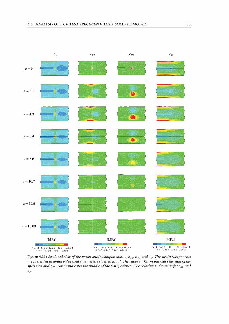
4.6. ANALYSIS OF DCB TEST SPECIMEN WITH A SOLID FE MODEL 73
-1.7e-3
-1e-3
-0.3e-3
0.3e-3
0.7e-3
1e-3
2e-3
2.5e-3
3..5e-3 -1e-3
-0.7e-3
-0.4e-3
-0.2e-3
-0.1e-3
0.1e-3
0.15e-3
0.2e-3
0.3e-3 -1.1e-3
-1e-3
-0.6e-3
-0.3e-3
0
0.1e-3
0.2e-3
0.3e-3
0.4e-3
εy εxz εy z εz
z = 0
z = 2.1
z = 4.3
z = 6.4
z = 8.6
z = 10.7
z = 12.9
z = 15.00
[MPa][MPa][MPa]
Figure 4.31: Sectional view of the tensor strain components εy , εxz , εy z and εz . The strain components
are presented as nodal values. All z values are given in [mm]. The value z = 0mm indicates the edge of the
specimen and z = 15mm indicates the middle of the test specimen. The colorbar is the same for εxz and
εy z .
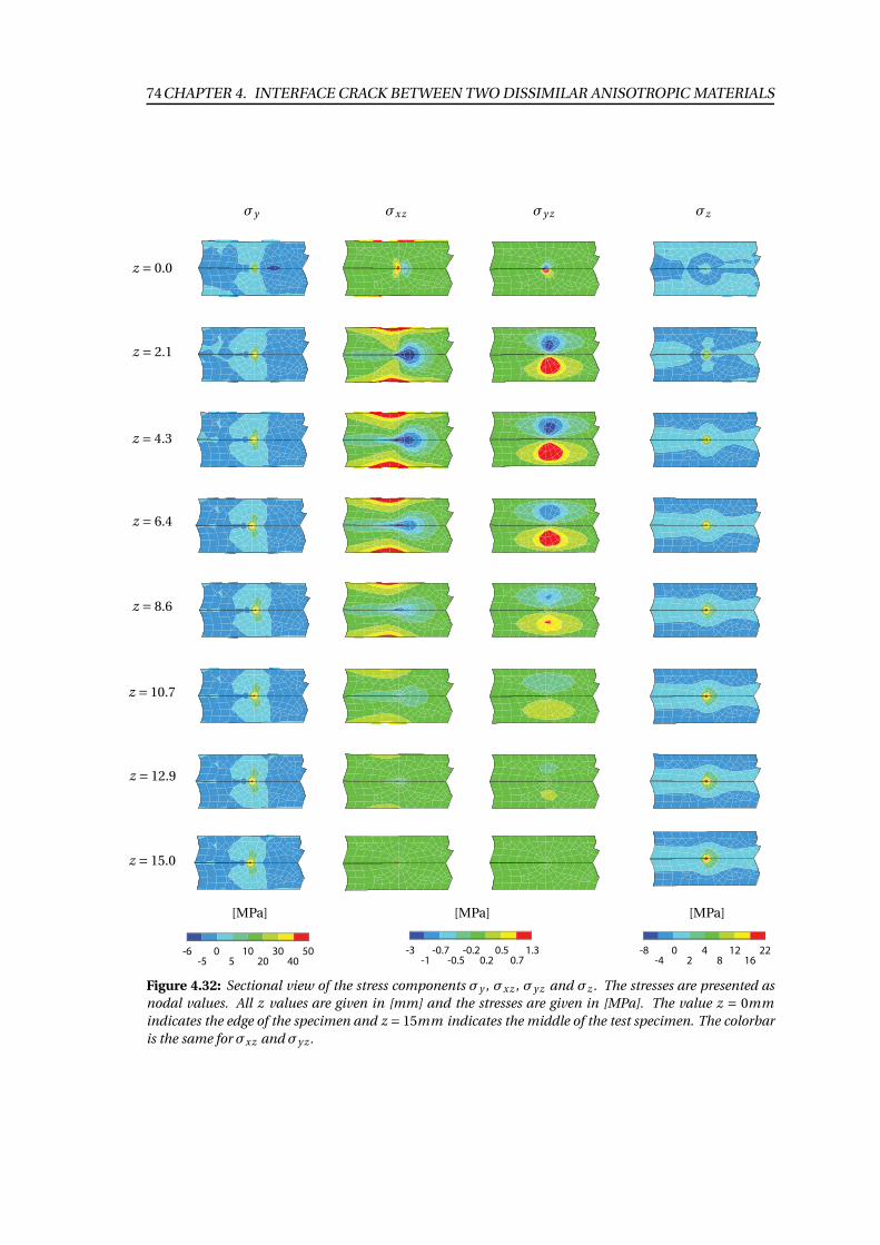
74CHAPTER 4. INTERFACE CRACK BETWEEN TWO DISSIMILAR ANISOTROPIC MATERIALS
-6
-5
0
5
10
20
30
40
50 -3
-1
-0.7
-0.5
-0.2
0.2
0.5
0.7
1.3 -8
-4
0
2
4
8
12
16
22
σy σxz σy z σz
z = 0.0
z = 2.1
z = 4.3
z = 6.4
z = 8.6
z = 10.7
z = 12.9
z = 15.0
[MPa][MPa][MPa]
Figure 4.32: Sectional view of the stress components σy , σxz , σy z and σz . The stresses are presented as
nodal values. All z values are given in [mm] and the stresses are given in [MPa]. The value z = 0mm
indicates the edge of the specimen and z = 15mm indicates the middle of the test specimen. The colorbar
is the same for σxz and σy z .
4.6. ANALYSIS OF DCB TEST SPECIMEN WITH A SOLID FE MODEL 75
The assumptions made in (Sørensen and Jacobsen, 2009) seem not to be fulfilled based on
the evaluation of the FE model of the test specimen. A summary of these assumptions and why
they are violated is seen in the lest below.
• Two dimensional structural response
From the displacement curves in figure 4.30 it is clear that due to the Poisson effects from
bending, the structural response can not be regarded as two dimensional.
• Plane strain
The strain and stress plots of the FE model of the test specimen in figure 4.31 and 4.32
show that it is not reasonable to assume plane strain nor plane stress through the width
of the specimen.
• Isotropic material
It seems from the orthotropic FE analysis that the elastic modulus E2 (and maybe also
E3) have a large influence on to what degree the relative crack face displacement is influ-
enced by the bending effects.
The fact that these assumptions seem not to be valid means that there are some significant
uncertainties related to the R-curves presented in Sørensen and Jacobsen (2009). This implies
that it is not reasonable to simulate R-curves for the solid FE model and compare these directly
to the R-curves in the article because a single R-curve cannot be obtained for three dimen-
sional cases with the method used in this project.
Thus in order to use the method on the solid model, it has to be further developed to make it
possible to vary the propagation of the crack front with respect to the z-coordinate. This has
not been done in this project, but is discussed in chapter 5.
4.6.2 Difference between R-curves for Solid FE model
A study of the difference between two R-curves determined for plane strain for relative dis-
placements on the edge and in the middle of the solid model for pure mode I loading has been
conducted. These curves are then compared to the R-curve from the test, in order to determine
which one is closest to the test results.
A R-curve similar to the one for mode I from the plane simulation is used for determining
the bridging law for the solid model. As this R-curve is used for the edge and the middle of the
specimen, this will lead to apparently different fracture resistances for the two cases.
Because the calculation of the J-integral is not valid for the three dimensional case, the R-
curves plotted for moment load instead of fracture resistance with respect to crack opening.
The loads from the test is obtained by solving for the moments, M1 and M2 in equation (4.33).
In the case of pure mode I M1 = M2.
In figure 4.33 the moment measured in the test is shown together with the moments pre-
dicted from the crack face displacement of the edge and middle, respectively. It is seen that
there is a good correspondence between the moment predicted for the crack face displace-
ments in the middle and the measured moment. On the contrary the moment determined
from the crack face displacement at the edge is far from the measured moment.
When the R-curves reach steady state there is approximately 30% difference between Mmeasured
and Medge. The difference between Mmeasured and Mmiddle is approximately -5%. From this
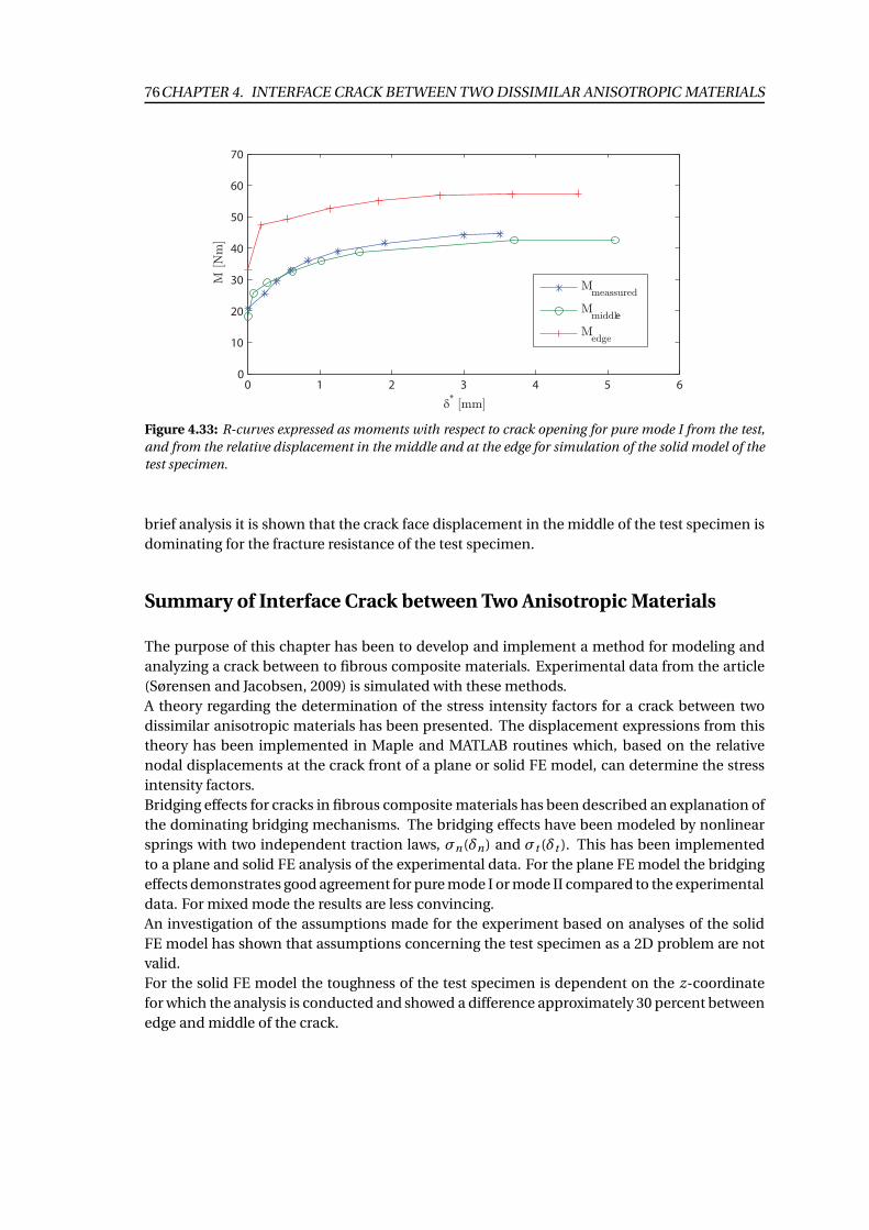
76CHAPTER 4. INTERFACE CRACK BETWEEN TWO DISSIMILAR ANISOTROPIC MATERIALS
0 1 2 3 4 5 60
10
20
30
40
50
60
70
M [N
m]
δ* [mm]
Mmeassured
Mmiddle
Medge
Figure 4.33: R-curves expressed as moments with respect to crack opening for pure mode I from the test,
and from the relative displacement in the middle and at the edge for simulation of the solid model of the
test specimen.
brief analysis it is shown that the crack face displacement in the middle of the test specimen is
dominating for the fracture resistance of the test specimen.
Summary of Interface Crack between Two Anisotropic Materials
The purpose of this chapter has been to develop and implement a method for modeling and
analyzing a crack between to fibrous composite materials. Experimental data from the article
(Sørensen and Jacobsen, 2009) is simulated with these methods.
A theory regarding the determination of the stress intensity factors for a crack between two
dissimilar anisotropic materials has been presented. The displacement expressions from this
theory has been implemented in Maple and MATLAB routines which, based on the relative
nodal displacements at the crack front of a plane or solid FE model, can determine the stress
intensity factors.
Bridging effects for cracks in fibrous composite materials has been described an explanation of
the dominating bridging mechanisms. The bridging effects have been modeled by nonlinear
springs with two independent traction laws, σn(δn) and σt (δt ). This has been implemented
to a plane and solid FE analysis of the experimental data. For the plane FE model the bridging
effects demonstrates good agreement for pure mode I or mode II compared to the experimental
data. For mixed mode the results are less convincing.
An investigation of the assumptions made for the experiment based on analyses of the solid
FE model has shown that assumptions concerning the test specimen as a 2D problem are not
valid.
For the solid FE model the toughness of the test specimen is dependent on the z-coordinate
for which the analysis is conducted and showed a difference approximately 30 percent between
edge and middle of the crack.
Chapter
5Discussion
The purpose of this chapter is to present and discuss suggested applications of the procedure
developed in this project. Furthermore, suggestions for further development of the mesh strategy,
bridging model and extension of the developed procedure for curved crack fronts, is presented.
5.1 Application of the Developed Procedure
In this section some applications of the developed procedure in the stage it has at the end of
the project period are described. These concern:
• Progressive crack modeling
• Modeling of test data
• Sub-modeling
• Plane crack simulation
5.1.1 Simulation of Progressive Crack Propagation
The main steps in the simulation procedure developed in this project for simulating progres-
sive crack propagation is illustrated in figure 5.1 and described below.
The simulation begins with a definition of the finite element model with a specification of
the geometry, the two materials on either side of the crack, loads on the structure and the length
and location of the initial crack without bridging between the crack faces. The expressions for
the relative displacements of the crack faces are calculated for either isotropic or anisotropic
materials, dependent on what type of materials are to be simulated.
When the definition of the model and the calculation of the displacement expressions are
conducted, the progressive simulation is initiated in a loop as indicated in figure 5.1. The finite
element model is analyzed and the relative nodal crack face displacements and the analytical
expression are exported to the parameter estimation in MATLAB. The stress intensity factors
K I and K I I are estimated, and by use of these the energy release rate G(K I ,K I I ) is calculated in
order to compare this to the critical fracture toughness Gc ,0 for the crack tip.
If G(K I ,K I I ) < Gc ,0 the crack is stable and the load can be increased, and the FE model is
solved for the increased load and the loop is repeated. If G(K I ,K I I ) >Gc ,0 the crack propagates
and must be increased a distance that is to be specified in the next run of the loop. A bridging
zone develops behind the crack tip, and this must be added into the FE model. Then the FE
77
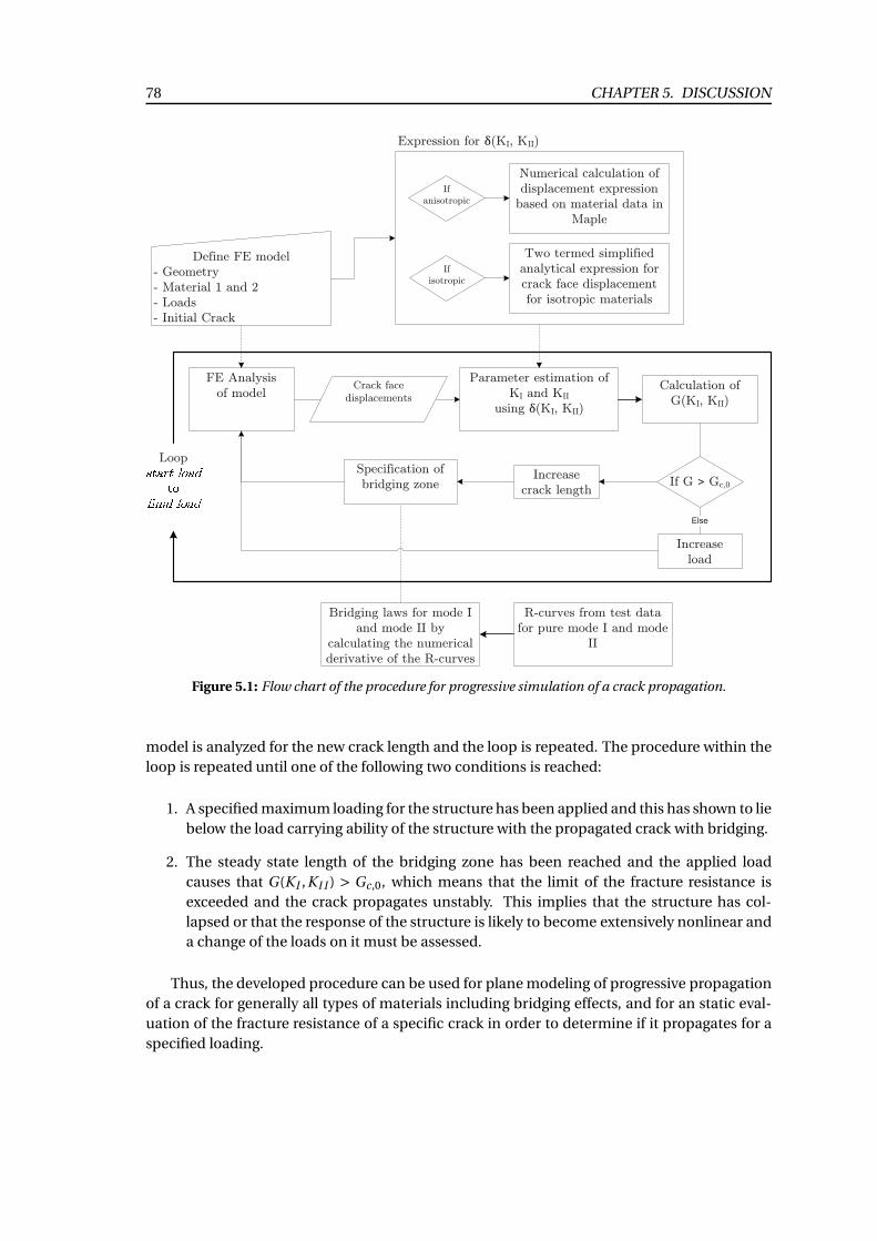
78 CHAPTER 5. DISCUSSION
FE Analysis of model
Parameter estimation of KI and KII
using (KI, KII)
Calculation of G(KI, KII)
Increase load
Increase crack length
Specification of bridging zone
R-curves from test data for pure mode I and mode
II
Bridging laws for mode I and mode II by
calculating the numerical derivative of the R-curves
Define FE model- Geometry- Material 1 and 2- Loads- Initial Crack
Crack face displacements
Expression for (KI, KII)
Numerical calculation of displacement expression
based on material data in Maple
Two termed simplified analytical expression for crack face displacement for isotropic materials
If anisotropic
If isotropic
Loop
If G Gc,0
Else
Figure 5.1: Flow chart of the procedure for progressive simulation of a crack propagation.
model is analyzed for the new crack length and the loop is repeated. The procedure within the
loop is repeated until one of the following two conditions is reached:
1. A specified maximum loading for the structure has been applied and this has shown to lie
below the load carrying ability of the structure with the propagated crack with bridging.
2. The steady state length of the bridging zone has been reached and the applied load
causes that G(K I ,K I I ) > Gc ,0, which means that the limit of the fracture resistance is
exceeded and the crack propagates unstably. This implies that the structure has col-
lapsed or that the response of the structure is likely to become extensively nonlinear and
a change of the loads on it must be assessed.
Thus, the developed procedure can be used for plane modeling of progressive propagation
of a crack for generally all types of materials including bridging effects, and for an static eval-
uation of the fracture resistance of a specific crack in order to determine if it propagates for a
specified loading.
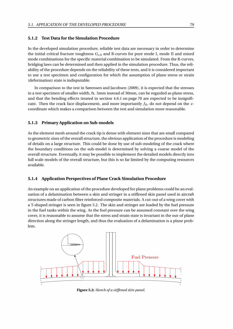
5.1. APPLICATION OF THE DEVELOPED PROCEDURE 79
5.1.2 Test Data for the Simulation Procedure
In the developed simulation procedure, reliable test data are necessary in order to determine
the initial critical fracture toughness Gc ,0 and R-curves for pure mode I, mode II and mixed
mode combinations for the specific material combination to be simulated. From the R-curves,
bridging laws can be determined and then applied in the simulation procedure. Thus, the reli-
ability of the procedure depends on the reliability of these tests, and it is considered important
to use a test specimen and configuration for which the assumption of plane stress or strain
(deformation) state is indisputable.
In comparison to the test in Sørensen and Jacobsen (2009), it is expected that the stresses
in a test specimen of smaller width, fx. 5mm instead of 30mm, can be regarded as plane stress,
and that the bending effects treated in section 4.6.1 on page 70 are expected to be insignifi-
cant. Then the crack face displacement, and more importantly JR , do not depend on the z-
coordinate which makes a comparison between the test and simulation more reasonable.
5.1.3 Primary Application on Sub-models
As the element mesh around the crack tip is dense with element sizes that are small compared
to geometric sizes of the overall structure, the obvious application of the procedure is modeling
of details on a large structure. This could be done by use of sub-modeling of the crack where
the boundary conditions on the sub-model is determined by solving a coarse model of the
overall structure. Eventually, it may be possible to implement the detailed models directly into
full scale models of the overall structure, but this is so far limited by the computing resources
available.
5.1.4 Application Perspectives of Plane Crack Simulation Procedure
An example on an application of the procedure developed for plane problems could be an eval-
uation of a delamination between a skin and stringer in a stiffened skin panel used in aircraft
structures made of carbon fiber reinforced composite materials. A cut-out of a wing cover with
a T-shaped stringer is seen in figure 5.2. The skin and stringer are loaded by the fuel pressure
in the fuel tanks within the wing. As the fuel pressure can be assumed constant over the wing
cover, it is reasonable to assume that the stress and strain state is invariant in the out-of plane
direction along the stringer length, and thus the evaluation of a delamination is a plane prob-
lem.
Fuel Pressure
Figure 5.2: Sketch of a stiffened skin panel.
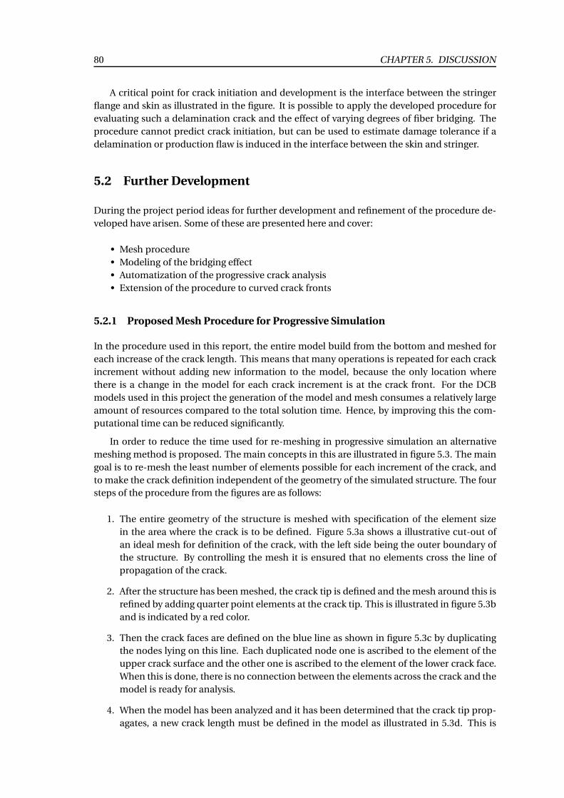
80 CHAPTER 5. DISCUSSION
A critical point for crack initiation and development is the interface between the stringer
flange and skin as illustrated in the figure. It is possible to apply the developed procedure for
evaluating such a delamination crack and the effect of varying degrees of fiber bridging. The
procedure cannot predict crack initiation, but can be used to estimate damage tolerance if a
delamination or production flaw is induced in the interface between the skin and stringer.
5.2 Further Development
During the project period ideas for further development and refinement of the procedure de-
veloped have arisen. Some of these are presented here and cover:
• Mesh procedure
• Modeling of the bridging effect
• Automatization of the progressive crack analysis
• Extension of the procedure to curved crack fronts
5.2.1 Proposed Mesh Procedure for Progressive Simulation
In the procedure used in this report, the entire model build from the bottom and meshed for
each increase of the crack length. This means that many operations is repeated for each crack
increment without adding new information to the model, because the only location where
there is a change in the model for each crack increment is at the crack front. For the DCB
models used in this project the generation of the model and mesh consumes a relatively large
amount of resources compared to the total solution time. Hence, by improving this the com-
putational time can be reduced significantly.
In order to reduce the time used for re-meshing in progressive simulation an alternative
meshing method is proposed. The main concepts in this are illustrated in figure 5.3. The main
goal is to re-mesh the least number of elements possible for each increment of the crack, and
to make the crack definition independent of the geometry of the simulated structure. The four
steps of the procedure from the figures are as follows:
1. The entire geometry of the structure is meshed with specification of the element size
in the area where the crack is to be defined. Figure 5.3a shows a illustrative cut-out of
an ideal mesh for definition of the crack, with the left side being the outer boundary of
the structure. By controlling the mesh it is ensured that no elements cross the line of
propagation of the crack.
2. After the structure has been meshed, the crack tip is defined and the mesh around this is
refined by adding quarter point elements at the crack tip. This is illustrated in figure 5.3b
and is indicated by a red color.
3. Then the crack faces are defined on the blue line as shown in figure 5.3c by duplicating
the nodes lying on this line. Each duplicated node one is ascribed to the element of the
upper crack surface and the other one is ascribed to the element of the lower crack face.
When this is done, there is no connection between the elements across the crack and the
model is ready for analysis.
4. When the model has been analyzed and it has been determined that the crack tip prop-
agates, a new crack length must be defined in the model as illustrated in 5.3d. This is
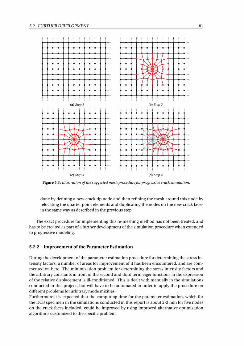
5.2. FURTHER DEVELOPMENT 81
(a) Step 1 (b) Step 2
(c) Step 3 (d) Step 4
Figure 5.3: Illustration of the suggested mesh procedure for progressive crack simulation.
done by defining a new crack tip node and then refining the mesh around this node by
relocating the quarter point elements and duplicating the nodes on the new crack faces
in the same way as described in the previous step.
The exact procedure for implementing this re-meshing method has not been treated, and
has to be created as part of a further development of the simulation procedure when extended
to progressive modeling.
5.2.2 Improvement of the Parameter Estimation
During the development of the parameter estimation procedure for determining the stress in-
tensity factors, a number of areas for improvement of it has been encountered, and are com-
mented on here. The minimization problem for determining the stress intensity factors and
the arbitrary constants in front of the second and third term eigenfunctions in the expression
of the relative displacement is ill-conditioned. This is dealt with manually in the simulations
conducted in this project, but will have to be automated in order to apply the procedure on
different problems for arbitrary mode mixities.
Furthermore it is expected that the computing time for the parameter estimation, which for
the DCB specimen in the simulations conducted in this report is about 2-3 min for five nodes
on the crack faces included, could be improved by using improved alternative optimization
algorithms customized to the specific problem.
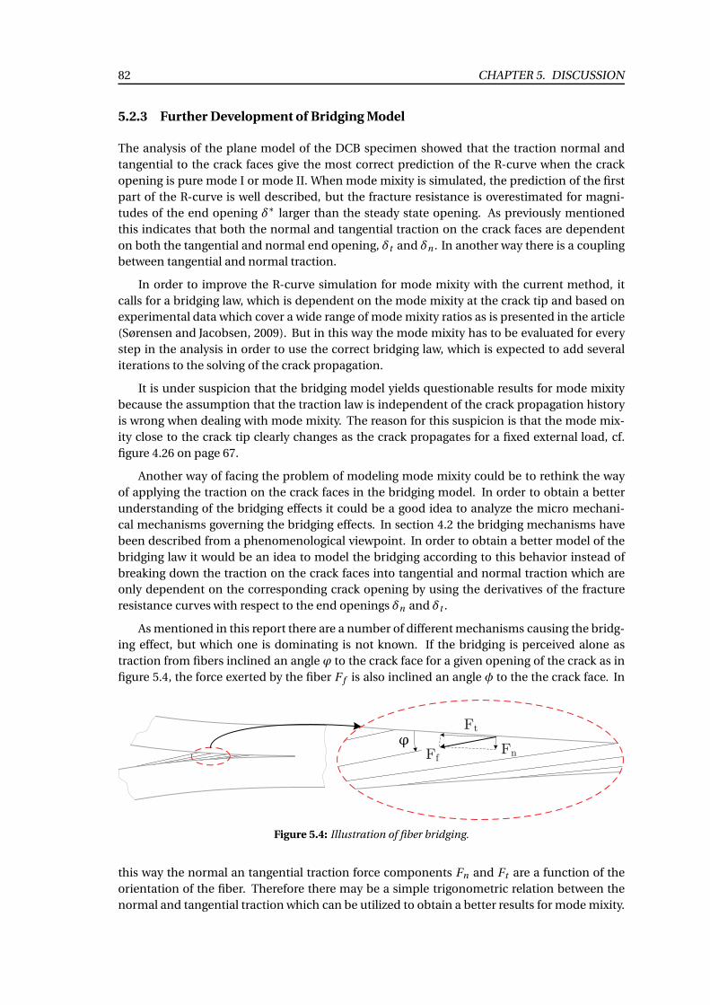
82 CHAPTER 5. DISCUSSION
5.2.3 Further Development of Bridging Model
The analysis of the plane model of the DCB specimen showed that the traction normal and
tangential to the crack faces give the most correct prediction of the R-curve when the crack
opening is pure mode I or mode II. When mode mixity is simulated, the prediction of the first
part of the R-curve is well described, but the fracture resistance is overestimated for magni-
tudes of the end opening δ∗ larger than the steady state opening. As previously mentioned
this indicates that both the normal and tangential traction on the crack faces are dependent
on both the tangential and normal end opening, δt and δn . In another way there is a coupling
between tangential and normal traction.
In order to improve the R-curve simulation for mode mixity with the current method, it
calls for a bridging law, which is dependent on the mode mixity at the crack tip and based on
experimental data which cover a wide range of mode mixity ratios as is presented in the article
(Sørensen and Jacobsen, 2009). But in this way the mode mixity has to be evaluated for every
step in the analysis in order to use the correct bridging law, which is expected to add several
iterations to the solving of the crack propagation.
It is under suspicion that the bridging model yields questionable results for mode mixity
because the assumption that the traction law is independent of the crack propagation history
is wrong when dealing with mode mixity. The reason for this suspicion is that the mode mix-
ity close to the crack tip clearly changes as the crack propagates for a fixed external load, cf.
figure 4.26 on page 67.
Another way of facing the problem of modeling mode mixity could be to rethink the way
of applying the traction on the crack faces in the bridging model. In order to obtain a better
understanding of the bridging effects it could be a good idea to analyze the micro mechani-
cal mechanisms governing the bridging effects. In section 4.2 the bridging mechanisms have
been described from a phenomenological viewpoint. In order to obtain a better model of the
bridging law it would be an idea to model the bridging according to this behavior instead of
breaking down the traction on the crack faces into tangential and normal traction which are
only dependent on the corresponding crack opening by using the derivatives of the fracture
resistance curves with respect to the end openings δn and δt .
As mentioned in this report there are a number of different mechanisms causing the bridg-
ing effect, but which one is dominating is not known. If the bridging is perceived alone as
traction from fibers inclined an angle ϕ to the crack face for a given opening of the crack as in
figure 5.4, the force exerted by the fiber F f is also inclined an angle φ to the the crack face. In
FfFn
Ft
Figure 5.4: Illustration of fiber bridging.
this way the normal an tangential traction force components Fn and Ft are a function of the
orientation of the fiber. Therefore there may be a simple trigonometric relation between the
normal and tangential traction which can be utilized to obtain a better results for mode mixity.
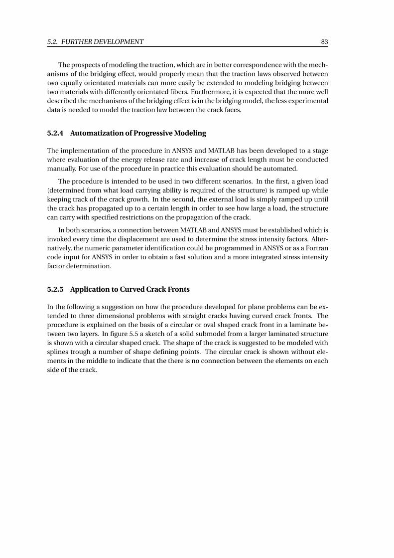
5.2. FURTHER DEVELOPMENT 83
The prospects of modeling the traction, which are in better correspondence with the mech-
anisms of the bridging effect, would properly mean that the traction laws observed between
two equally orientated materials can more easily be extended to modeling bridging between
two materials with differently orientated fibers. Furthermore, it is expected that the more well
described the mechanisms of the bridging effect is in the bridging model, the less experimental
data is needed to model the traction law between the crack faces.
5.2.4 Automatization of Progressive Modeling
The implementation of the procedure in ANSYS and MATLAB has been developed to a stage
where evaluation of the energy release rate and increase of crack length must be conducted
manually. For use of the procedure in practice this evaluation should be automated.
The procedure is intended to be used in two different scenarios. In the first, a given load
(determined from what load carrying ability is required of the structure) is ramped up while
keeping track of the crack growth. In the second, the external load is simply ramped up until
the crack has propagated up to a certain length in order to see how large a load, the structure
can carry with specified restrictions on the propagation of the crack.
In both scenarios, a connection between MATLAB and ANSYS must be established which is
invoked every time the displacement are used to determine the stress intensity factors. Alter-
natively, the numeric parameter identification could be programmed in ANSYS or as a Fortran
code input for ANSYS in order to obtain a fast solution and a more integrated stress intensity
factor determination.
5.2.5 Application to Curved Crack Fronts
In the following a suggestion on how the procedure developed for plane problems can be ex-
tended to three dimensional problems with straight cracks having curved crack fronts. The
procedure is explained on the basis of a circular or oval shaped crack front in a laminate be-
tween two layers. In figure 5.5 a sketch of a solid submodel from a larger laminated structure
is shown with a circular shaped crack. The shape of the crack is suggested to be modeled with
splines trough a number of shape defining points. The circular crack is shown without ele-
ments in the middle to indicate that the there is no connection between the elements on each
side of the crack.
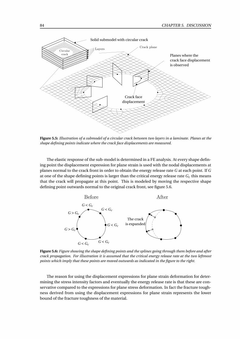
84 CHAPTER 5. DISCUSSION
Circular crack
LayersCrack plane
Crack face
displacement
Planes where the
crack face displacement
is observed
Solid submodel with circular crack
Figure 5.5: Illustration of a submodel of a circular crack between two layers in a laminate. Planes at the
shape defining points indicate where the crack face displacements are measured.
The elastic response of the sub-model is determined in a FE analysis. At every shape defin-
ing point the displacement expression for plane strain is used with the nodal displacements at
planes normal to the crack front in order to obtain the energy release rate G at each point. If G
at one of the shape defining points is larger than the critical energy release rate Gc this means
that the crack will propagate at this point. This is modeled by moving the respective shape
defining point outwards normal to the original crack front, see figure 5.6.
Before After
G <Gc
G <Gc
G <GcG <Gc
G <Gc
G >Gc
G >Gc
The crack
is expanded
Figure 5.6: Figure showing the shape defining points and the splines going through them before and after
crack propagation. For illustration it is assumed that the critical energy release rate at the two leftmost
points which imply that these points are moved outwards as indicated in the figure to the right.
The reason for using the displacement expressions for plane strain deformation for deter-
mining the stress intensity factors and eventually the energy release rate is that these are con-
servative compared to the expressions for plane stress deformation. In fact the fracture tough-
ness derived from using the displacement expressions for plane strain represents the lower
bound of the fracture toughness of the material.
5.2. FURTHER DEVELOPMENT 85
When considering three dimensional fracture mechanical problems in the way described
above, different areas of the modeling procedure for plane problems needs to be generalized
to three dimensions. This involves for example:
• Traction laws that take the fiber orientation with respect to the crack front into considera-
tion. This could strengthen the argument for choosing a more physically correct bridging
model as mention in subsection 5.2.3.
• The compliance matrices used in the displacement expressions for anisotropic materials
are needed in the coordinate system following the normal to the crack front. This means
that the compliance matrix used in the displacement expressions in general is unique
for each location on the crack front due to the coordinate transformation. This implies
that numeric calculations of the displacement expressions for each location of the shape
defining points has to be performed.

Conclusion
In this project a numerical procedure for determining if an interface crack between two dis-
similar materials propagates for a specific outer load has been developed. This has been done
in three main steps concerning a crack in a simple isotropic material, an interface crack in
an isotropic bimaterial and an anisotropic bimaterial. This procedure applies a full fracture
mechanical formulation for relative displacements of the crack surfaces near the crack tip to
estimate the stress intensity factors. These are used to calculate the energy release rate and
this is compared to a material dependent critical value in order to determine if the crack tip
propagates.
An effort has been made for gaining a considerable understanding of the theory of fracture
mechanics for describing stresses and displacements around the crack tip interface cracks in
dissimilar materials. Particular focus has been on the derivation of complex stress and dis-
placement for the isotropic bimaterial interface crack, involving a determination of complex
potentials from crack boundary conditions. A theory on a description of the full field solution
for an interface crack in an isotropic bimaterial has been treated and interpreted with applica-
tion of it kept in mind.
The fracture mechanical expressions for the crack face displacements have been imple-
mented in a numerical curve fit method which is used to determine the stress intensity factors
from the nodal crack face displacements from a FE model. It has been made possible to use
nodal displacement values a distance away from the crack tip that is 10-20 times larger than if
only the first eigenfunction solution is used. This is done by applying two and three eigenfunc-
tions in a simplified form in the expression for the crack face displacements.
The curve fit of the analytical expression to finite element results has been programmed as a
least squares fit for the two bimaterial cases using the conjugate gradient method to estimate
the stress intensity factors and a weighting factor for each of the simplified eigenfunctions.
The theory for anisotropic materials is used for simulating an interface crack between two
orthotropic unidirectional fiber materials, and for this type of materials large scale bridging of
fibers between the crack faces tend to cause a significant increase of the overall fracture resis-
tance as the crack propagates. Dominating mechanisms causing fiber bridging has been de-
scribed and a modeling of this by using nonlinear springs with specified traction-displacement
descriptions has been implemented in a plane and a solid finite element model.
The capability for estimating propagation of a crack with bridging fibers of the developed
procedure has been demonstrated for a plane model of two similar orthotropic materials. This
has been done by applying bridging laws obtained from an R-curve based on test data, and
comparing simulated R-curves with R-curves from the test. This has shown that for pure mode
I and II it is possible to simulate the tested increase in the fracture resistance to a satisfactory
degree (figures 4.23 and 4.25 on page 66-67), whereas for a mixed mode case the results are less
convincing and has to be developed further (figure 4.27 on page 68).
The stress and strain state through the width of a solid model of a double cantilever beam
specimen for two similar orthotropic materials used in the test in (Sørensen and Jacobsen,
2009) has been analyzed. It is shown that the assumptions regarding the specimen as a plane
problem made in the article seem not to be valid. This is because the stress and strain state in
87

88 CHAPTER 5. DISCUSSION
the specimen varies significantly through the width and that the crack face displacement are
80% larger in the middle than at the edges for the specific specimen. A R-curve from the test
for pure mode I has been compared to R-curves simulated for the middle and the edge of the
specimen, and this shows that it corresponds to the one in the middle.
Bibliography
Andreasen, J. H. (2008). Brudmekanik. Department of Mechanical Engineering.
Arora, Jasbir (2004). Introduction to Optimum Design. 2nd ed.. Academic Press.
Bao, G. and Z. Suo (1992). Remarks on crack-bridging concepts. Applied Mechanics Reviews 45(8), 355–366.
Barsoum, Roshdy S. (1977). Triangular quarter-point elements as elastic and perfectly-plastic crack tip elements.
International Journal for Numerical Methods in Engineering 11(1), 85–98.
Hansen, A. L. (2009). Simulation of crack growth and r-curve behavior using cohesive zone modeling.
Hutchinson, John W., Viggo Tvergaard and Fariborz Ghahremani (1990). Three-dimensional effects in microcrack
nucleation in brittle polycrystals. Journal of the American Ceramic Society 73(6), 1548–1554.
Kildegaard, Arne (2002). Kompendium i Brudmekanik. Department of Mechanical Engineering.
Kreyszig, Erwin (2005). Advanced Engineering Mathematics. Wiley.
Lekhnitskii, S. G. (1981). Theory of Elasticity of an Anisotropic Body. Mir Publishers.
Lekhnitskii, Sergei G. (1968). Anisotropic Plates. second ed.
Muskhelishvili, N. I. (1977). Some Basic Problems of the Mathematical Theory of Elasticity. 1 ed.. Springer.
Rathkjen, A. (1984). Plan elasticitetsteori og komplekse variable. second ed.. Aalborg University.
Rice, J.R. (1968). A path independent integral and the approximate analysis of strain concentration by notches and
cracks. Journal of Applied Mechanics 35, 379–386.
Sørensen, Bent F. and Torben K. Jacobsen (2009). Characterizing delamination of fibre composites by mixed mode
cohesive laws. Composites Science and Technology.
Sørensen, Bent, Kenneth Jørgensen, Torben Jacobsen and Rasmus Østergaard (2006). Dcb-specimen loaded with
uneven bending moments. International Journal of Fracture 141(1), 163–176.
Spearing, S.M. and A.G. Evans (1992). The role of fiber bridging in the delamination resistance of fiber-reinforced
composites. Acta Metallurgica et Materialia 40(9), 2191 – 2199.
Sørensen, Bent F. and Torben K. Jacobsen (1998). Large-scale bridging in composites: R-curves and bridging laws.
Composites Part A: Applied Science and Manufacturing 29(11), 1443 – 1451.
Sørensen, Bent F., Stergios Goutianos and Torben K. Jacobsen (2009). Strength scaling of adhesive joints in polymer-
matrix composites. International Journal of Solids and Structures 46(3-4), 741 – 761.
Suo, Zhigang (1990). Singularities, interfaces and cracks in dissimilar anisotropic media. Proceedings of the Royal
Society of London. Series A, Mathematical and Physical Sciences 427(1873), 331–358.
Suo, Zhigang and John W. Hutchinson (1990). Interface crack between two elastic layers. International Journal of
Fracture 43(1), 1–18.
Williams, M. L. (1959). The stresses around a fault or crack in dissimilar media. Bulletin of the Seismological Society
of America 49(2), 199–204.
89


APPENDIX
91

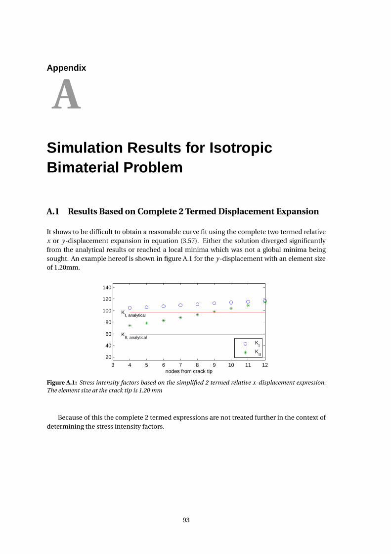
Appendix
ASimulation Results for IsotropicBimaterial Problem
A.1 Results Based on Complete 2 Termed Displacement Expansion
It shows to be difficult to obtain a reasonable curve fit using the complete two termed relative
x or y-displacement expansion in equation (3.57). Either the solution diverged significantly
from the analytical results or reached a local minima which was not a global minima being
sought. An example hereof is shown in figure A.1 for the y-displacement with an element size
of 1.20mm.
3 4 5 6 7 8 9 10 11 12
20
40
60
80
100
120
140
nodes from crack tip
KI, analytical
KII, analytical
KI
KII
Figure A.1: Stress intensity factors based on the simplified 2 termed relative x-displacement expression.
The element size at the crack tip is 1.20 mm
Because of this the complete 2 termed expressions are not treated further in the context of
determining the stress intensity factors.
93
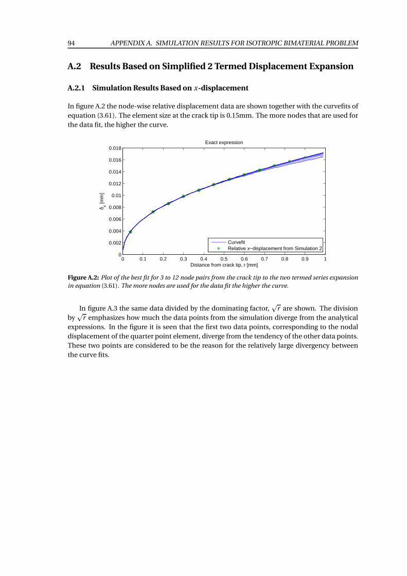
94 APPENDIX A. SIMULATION RESULTS FOR ISOTROPIC BIMATERIAL PROBLEM
A.2 Results Based on Simplified 2 Termed Displacement Expansion
A.2.1 Simulation Results Based on x-displacement
In figure A.2 the node-wise relative displacement data are shown together with the curvefits of
equation (3.61). The element size at the crack tip is 0.15mm. The more nodes that are used for
the data fit, the higher the curve.
0 0.1 0.2 0.3 0.4 0.5 0.6 0.7 0.8 0.9 10
0.002
0.004
0.006
0.008
0.01
0.012
0.014
0.016
0.018
Distance from crack tip, r [mm]
δ x [mm
]
Exact expression
CurvefitRelative x−displacement from Simulation 2
Figure A.2: Plot of the best fit for 3 to 12 node pairs from the crack tip to the two termed series expansion
in equation (3.61). The more nodes are used for the data fit the higher the curve.
In figure A.3 the same data divided by the dominating factor,p
r are shown. The division
byp
r emphasizes how much the data points from the simulation diverge from the analytical
expressions. In the figure it is seen that the first two data points, corresponding to the nodal
displacement of the quarter point element, diverge from the tendency of the other data points.
These two points are considered to be the reason for the relatively large divergency between
the curve fits.
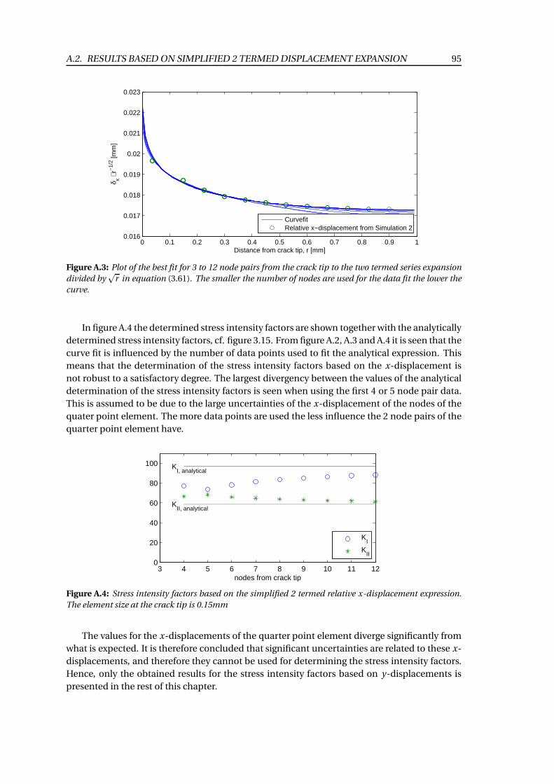
A.2. RESULTS BASED ON SIMPLIFIED 2 TERMED DISPLACEMENT EXPANSION 95
0 0.1 0.2 0.3 0.4 0.5 0.6 0.7 0.8 0.9 10.016
0.017
0.018
0.019
0.02
0.021
0.022
0.023
Distance from crack tip, r [mm]
δ x ⋅ r−
1/2 [m
m]
CurvefitRelative x−displacement from Simulation 2
Figure A.3: Plot of the best fit for 3 to 12 node pairs from the crack tip to the two termed series expansion
divided byp
r in equation (3.61). The smaller the number of nodes are used for the data fit the lower the
curve.
In figure A.4 the determined stress intensity factors are shown together with the analytically
determined stress intensity factors, cf. figure 3.15. From figure A.2, A.3 and A.4 it is seen that the
curve fit is influenced by the number of data points used to fit the analytical expression. This
means that the determination of the stress intensity factors based on the x-displacement is
not robust to a satisfactory degree. The largest divergency between the values of the analytical
determination of the stress intensity factors is seen when using the first 4 or 5 node pair data.
This is assumed to be due to the large uncertainties of the x-displacement of the nodes of the
quater point element. The more data points are used the less influence the 2 node pairs of the
quarter point element have.
3 4 5 6 7 8 9 10 11 120
20
40
60
80
100
nodes from crack tip
KI, analytical
KII, analytical
KI
KII
Figure A.4: Stress intensity factors based on the simplified 2 termed relative x-displacement expression.
The element size at the crack tip is 0.15mm
The values for the x-displacements of the quarter point element diverge significantly from
what is expected. It is therefore concluded that significant uncertainties are related to these x-
displacements, and therefore they cannot be used for determining the stress intensity factors.
Hence, only the obtained results for the stress intensity factors based on y-displacements is
presented in the rest of this chapter.
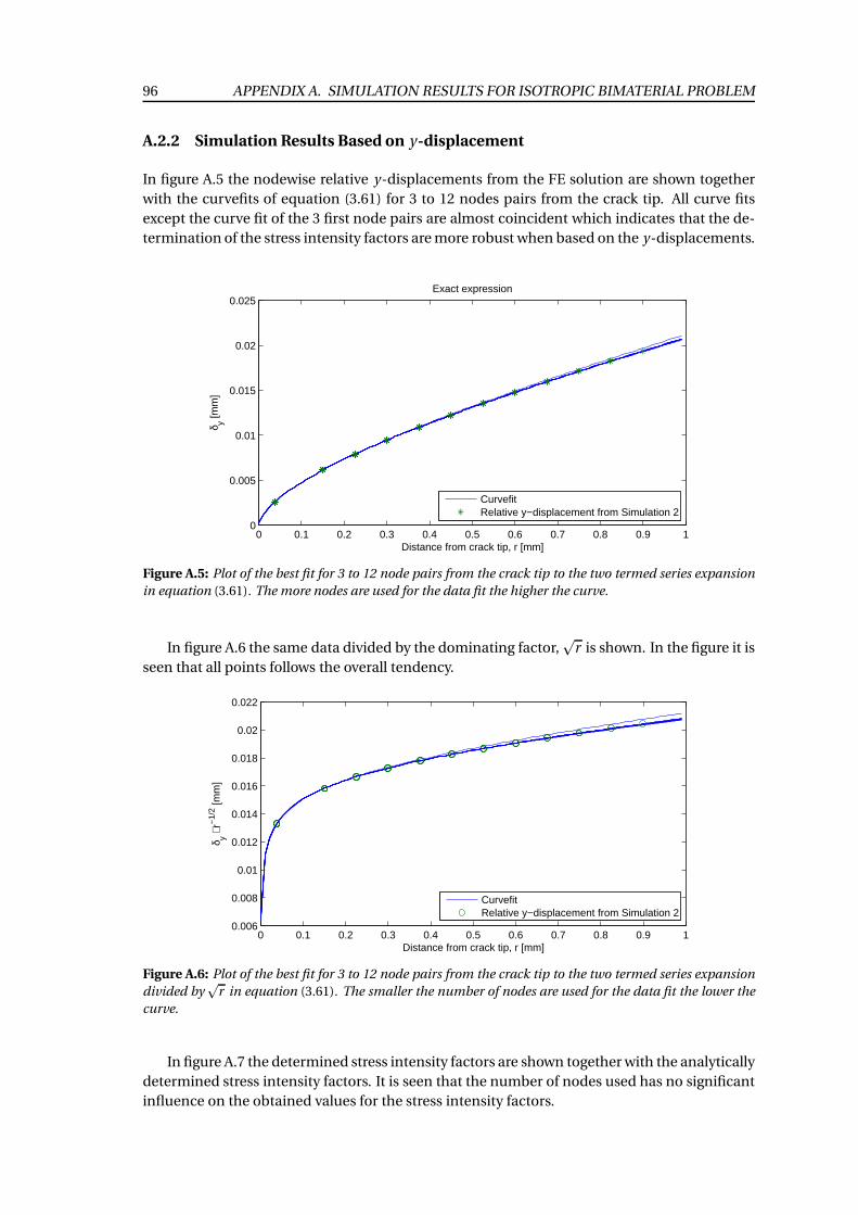
96 APPENDIX A. SIMULATION RESULTS FOR ISOTROPIC BIMATERIAL PROBLEM
A.2.2 Simulation Results Based on y-displacement
In figure A.5 the nodewise relative y-displacements from the FE solution are shown together
with the curvefits of equation (3.61) for 3 to 12 nodes pairs from the crack tip. All curve fits
except the curve fit of the 3 first node pairs are almost coincident which indicates that the de-
termination of the stress intensity factors are more robust when based on the y-displacements.
0 0.1 0.2 0.3 0.4 0.5 0.6 0.7 0.8 0.9 10
0.005
0.01
0.015
0.02
0.025
Distance from crack tip, r [mm]
δ y [mm
]
Exact expression
CurvefitRelative y−displacement from Simulation 2
Figure A.5: Plot of the best fit for 3 to 12 node pairs from the crack tip to the two termed series expansion
in equation (3.61). The more nodes are used for the data fit the higher the curve.
In figure A.6 the same data divided by the dominating factor,p
r is shown. In the figure it is
seen that all points follows the overall tendency.
0 0.1 0.2 0.3 0.4 0.5 0.6 0.7 0.8 0.9 10.006
0.008
0.01
0.012
0.014
0.016
0.018
0.02
0.022
Distance from crack tip, r [mm]
δ y ⋅ r−
1/2 [m
m]
CurvefitRelative y−displacement from Simulation 2
Figure A.6: Plot of the best fit for 3 to 12 node pairs from the crack tip to the two termed series expansion
divided byp
r in equation (3.61). The smaller the number of nodes are used for the data fit the lower the
curve.
In figure A.7 the determined stress intensity factors are shown together with the analytically
determined stress intensity factors. It is seen that the number of nodes used has no significant
influence on the obtained values for the stress intensity factors.
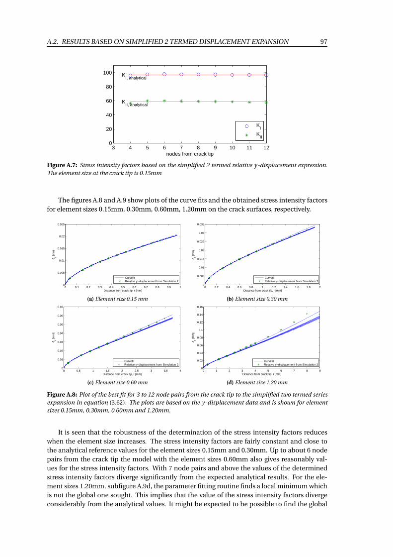
A.2. RESULTS BASED ON SIMPLIFIED 2 TERMED DISPLACEMENT EXPANSION 97
3 4 5 6 7 8 9 10 11 120
20
40
60
80
100
nodes from crack tip
KI, analytical
KII, analytical
KI
KII
Figure A.7: Stress intensity factors based on the simplified 2 termed relative y-displacement expression.
The element size at the crack tip is 0.15mm
The figures A.8 and A.9 show plots of the curve fits and the obtained stress intensity factors
for element sizes 0.15mm, 0.30mm, 0.60mm, 1.20mm on the crack surfaces, respectively.
0 0.1 0.2 0.3 0.4 0.5 0.6 0.7 0.8 0.9 10
0.005
0.01
0.015
0.02
0.025
Distance from crack tip, r [mm]
δ y [mm
]
CurvefitRelative y−displacement from Simulation 2
(a) Element size 0.15 mm
0 0.2 0.4 0.6 0.8 1 1.2 1.4 1.6 1.8 20
0.005
0.01
0.015
0.02
0.025
0.03
0.035
Distance from crack tip, r [mm]
δ y [mm
]
CurvefitRelative y−displacement from Simulation 2
(b) Element size 0.30 mm
0 0.5 1 1.5 2 2.5 3 3.5 40
0.01
0.02
0.03
0.04
0.05
0.06
0.07
Distance from crack tip, r [mm]
δ y [mm
]
CurvefitRelative y−displacement from Simulation 2
(c) Element size 0.60 mm
0 1 2 3 4 5 6 7 8 90
0.02
0.04
0.06
0.08
0.1
0.12
0.14
0.16
Distance from crack tip, r [mm]
δ y [mm
]
CurvefitRelative y−displacement from Simulation 2
(d) Element size 1.20 mm
Figure A.8: Plot of the best fit for 3 to 12 node pairs from the crack tip to the simplified two termed series
expansion in equation (3.62). The plots are based on the y-displacement data and is shown for element
sizes 0.15mm, 0.30mm, 0.60mm and 1.20mm.
It is seen that the robustness of the determination of the stress intensity factors reduces
when the element size increases. The stress intensity factors are fairly constant and close to
the analytical reference values for the element sizes 0.15mm and 0.30mm. Up to about 6 node
pairs from the crack tip the model with the element sizes 0.60mm also gives reasonably val-
ues for the stress intensity factors. With 7 node pairs and above the values of the determined
stress intensity factors diverge significantly from the expected analytical results. For the ele-
ment sizes 1.20mm, subfigure A.9d, the parameter fitting routine finds a local minimum which
is not the global one sought. This implies that the value of the stress intensity factors diverge
considerably from the analytical values. It might be expected to be possible to find the global
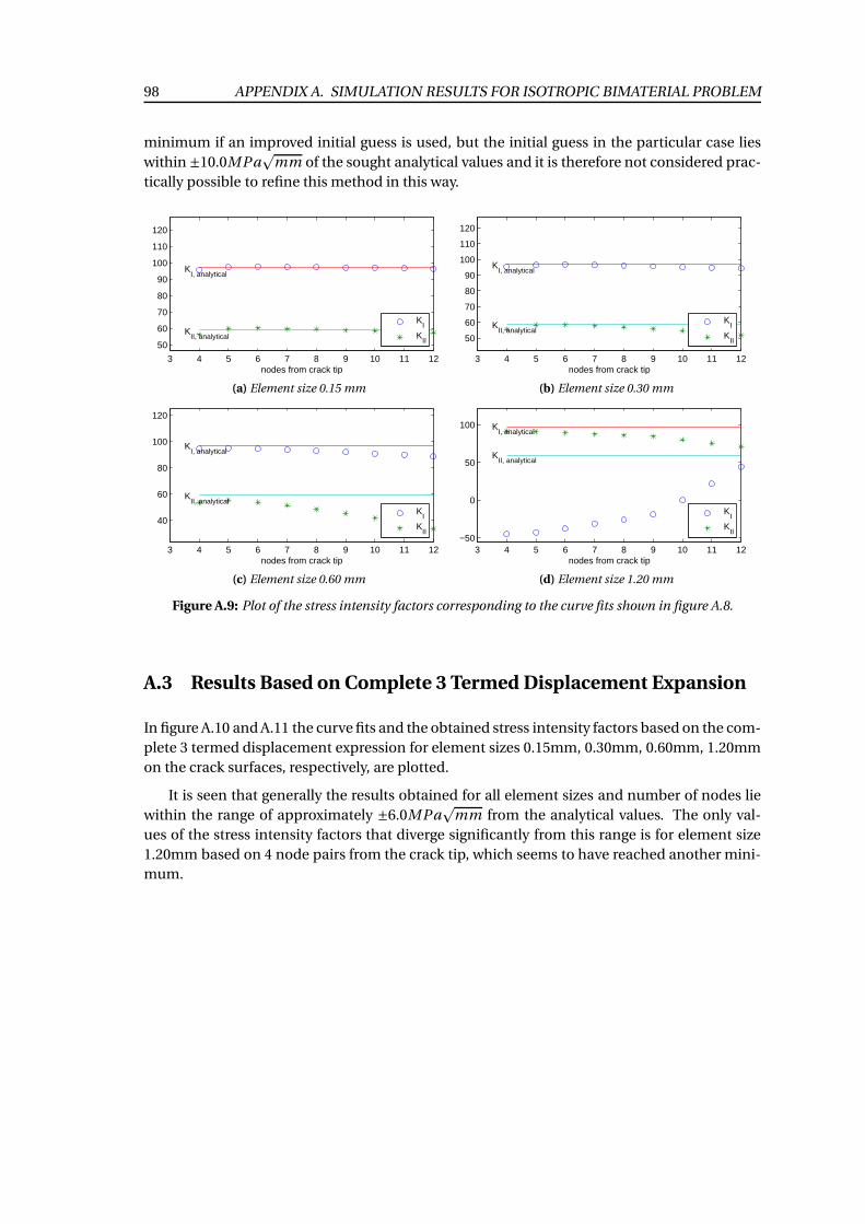
98 APPENDIX A. SIMULATION RESULTS FOR ISOTROPIC BIMATERIAL PROBLEM
minimum if an improved initial guess is used, but the initial guess in the particular case lies
within ±10.0MPap
mm of the sought analytical values and it is therefore not considered prac-
tically possible to refine this method in this way.
3 4 5 6 7 8 9 10 11 12
50
60
70
80
90
100
110
120
nodes from crack tip
KI, analytical
KII, analytical
KI
KII
(a) Element size 0.15 mm
3 4 5 6 7 8 9 10 11 12
50
60
70
80
90
100
110
120
nodes from crack tip
KI, analytical
KII, analytical
KI
KII
(b) Element size 0.30 mm
3 4 5 6 7 8 9 10 11 12
40
60
80
100
120
nodes from crack tip
KI, analytical
KII, analytical
KI
KII
(c) Element size 0.60 mm
3 4 5 6 7 8 9 10 11 12−50
0
50
100
nodes from crack tip
KI, analytical
KII, analytical
KI
KII
(d) Element size 1.20 mm
Figure A.9: Plot of the stress intensity factors corresponding to the curve fits shown in figure A.8.
A.3 Results Based on Complete 3 Termed Displacement Expansion
In figure A.10 and A.11 the curve fits and the obtained stress intensity factors based on the com-
plete 3 termed displacement expression for element sizes 0.15mm, 0.30mm, 0.60mm, 1.20mm
on the crack surfaces, respectively, are plotted.
It is seen that generally the results obtained for all element sizes and number of nodes lie
within the range of approximately ±6.0MPap
mm from the analytical values. The only val-
ues of the stress intensity factors that diverge significantly from this range is for element size
1.20mm based on 4 node pairs from the crack tip, which seems to have reached another mini-
mum.
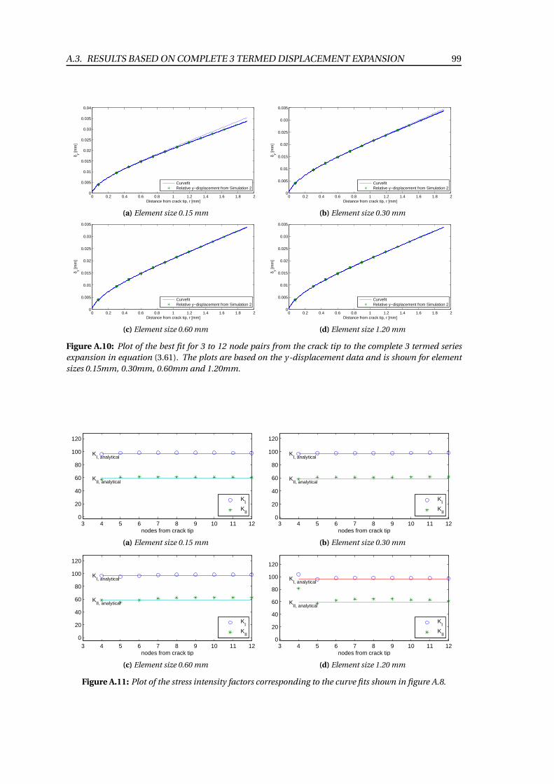
A.3. RESULTS BASED ON COMPLETE 3 TERMED DISPLACEMENT EXPANSION 99
0 0.2 0.4 0.6 0.8 1 1.2 1.4 1.6 1.8 20
0.005
0.01
0.015
0.02
0.025
0.03
0.035
0.04
Distance from crack tip, r [mm]
δ y [mm
]
CurvefitRelative y−displacement from Simulation 2
(a) Element size 0.15 mm
0 0.2 0.4 0.6 0.8 1 1.2 1.4 1.6 1.8 20
0.005
0.01
0.015
0.02
0.025
0.03
0.035
Distance from crack tip, r [mm]
δ y [mm
]
CurvefitRelative y−displacement from Simulation 2
(b) Element size 0.30 mm
0 0.2 0.4 0.6 0.8 1 1.2 1.4 1.6 1.8 20
0.005
0.01
0.015
0.02
0.025
0.03
0.035
Distance from crack tip, r [mm]
δ y [mm
]
CurvefitRelative y−displacement from Simulation 2
(c) Element size 0.60 mm
0 0.2 0.4 0.6 0.8 1 1.2 1.4 1.6 1.8 20
0.005
0.01
0.015
0.02
0.025
0.03
0.035
Distance from crack tip, r [mm]
δ y [mm
]
CurvefitRelative y−displacement from Simulation 2
(d) Element size 1.20 mm
Figure A.10: Plot of the best fit for 3 to 12 node pairs from the crack tip to the complete 3 termed series
expansion in equation (3.61). The plots are based on the y-displacement data and is shown for element
sizes 0.15mm, 0.30mm, 0.60mm and 1.20mm.
3 4 5 6 7 8 9 10 11 120
20
40
60
80
100
120
nodes from crack tip
KI, analytical
KII, analytical
KI
KII
(a) Element size 0.15 mm
3 4 5 6 7 8 9 10 11 120
20
40
60
80
100
120
nodes from crack tip
KI, analytical
KII, analytical
KI
KII
(b) Element size 0.30 mm
3 4 5 6 7 8 9 10 11 120
20
40
60
80
100
120
nodes from crack tip
KI, analytical
KII, analytical
KI
KII
(c) Element size 0.60 mm
3 4 5 6 7 8 9 10 11 120
20
40
60
80
100
120
nodes from crack tip
KI, analytical
KII, analytical
KI
KII
(d) Element size 1.20 mm
Figure A.11: Plot of the stress intensity factors corresponding to the curve fits shown in figure A.8.
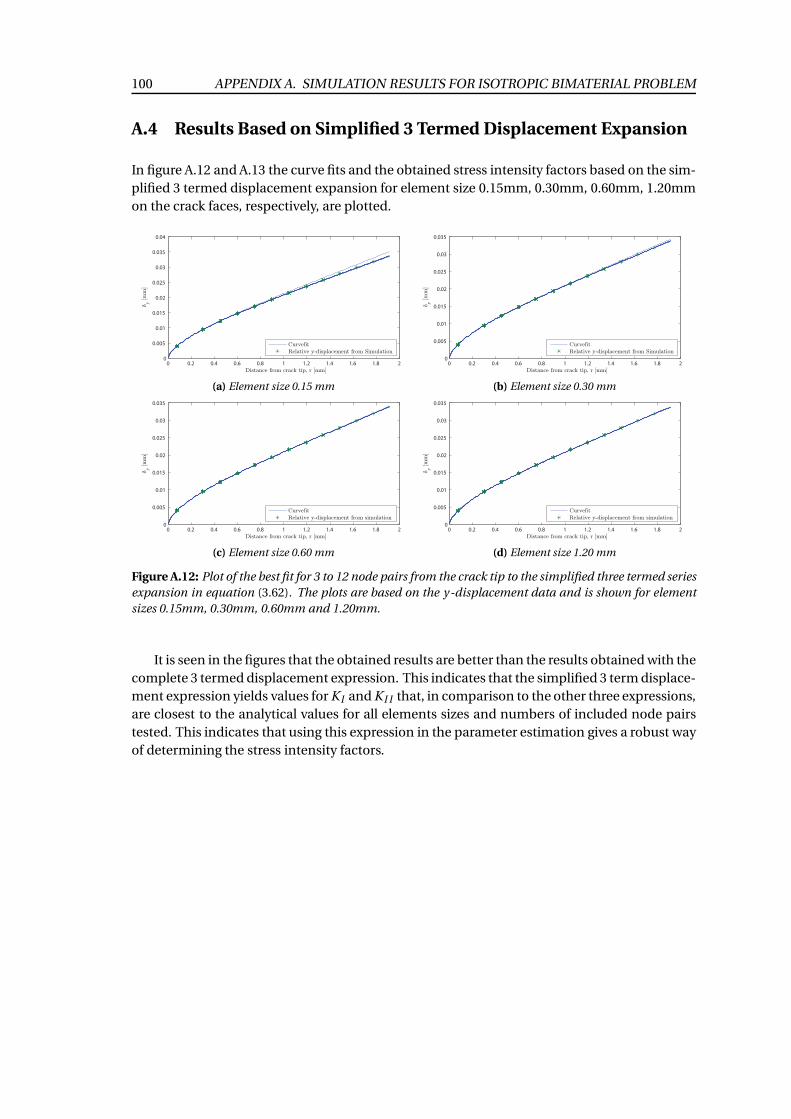
100 APPENDIX A. SIMULATION RESULTS FOR ISOTROPIC BIMATERIAL PROBLEM
A.4 Results Based on Simplified 3 Termed Displacement Expansion
In figure A.12 and A.13 the curve fits and the obtained stress intensity factors based on the sim-
plified 3 termed displacement expansion for element size 0.15mm, 0.30mm, 0.60mm, 1.20mm
on the crack faces, respectively, are plotted.
0 0.2 0.4 0.6 0.8 1 1.2 1.4 1.6 1.8 20
0.005
0.01
0.015
0.02
0.025
0.03
0.035
0.04
Distance from crack tip, r [mm]
δy [
mm
]
CurvefitRelative y-displacement from Simulation
(a) Element size 0.15 mm
0 0.2 0.4 0.6 0.8 1 1.2 1.4 1.6 1.8 20
0.005
0.01
0.015
0.02
0.025
0.03
0.035
Distance from crack tip, r [mm]
δy [
mm
]
CurvefitRelative y-displacement from Simulation
(b) Element size 0.30 mm
0 0.2 0.4 0.6 0.8 1 1.2 1.4 1.6 1.8 20
0.005
0.01
0.015
0.02
0.025
0.03
0.035
Distance from crack tip, r [mm]
δy [
mm
]
CurvefitRelative y-displacement from simulation
(c) Element size 0.60 mm
0 0.2 0.4 0.6 0.8 1 1.2 1.4 1.6 1.8 20
0.005
0.01
0.015
0.02
0.025
0.03
0.035
Distance from crack tip, r [mm]
δy [
mm
]
CurvefitRelative y-displacement from simulation
(d) Element size 1.20 mm
Figure A.12: Plot of the best fit for 3 to 12 node pairs from the crack tip to the simplified three termed series
expansion in equation (3.62). The plots are based on the y-displacement data and is shown for element
sizes 0.15mm, 0.30mm, 0.60mm and 1.20mm.
It is seen in the figures that the obtained results are better than the results obtained with the
complete 3 termed displacement expression. This indicates that the simplified 3 term displace-
ment expression yields values for K I and K I I that, in comparison to the other three expressions,
are closest to the analytical values for all elements sizes and numbers of included node pairs
tested. This indicates that using this expression in the parameter estimation gives a robust way
of determining the stress intensity factors.
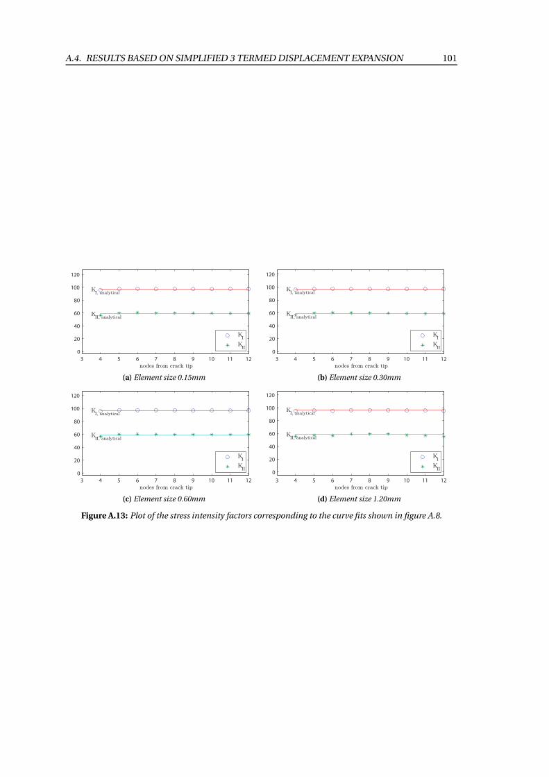
A.4. RESULTS BASED ON SIMPLIFIED 3 TERMED DISPLACEMENT EXPANSION 101
3 4 5 6 7 8 9 10 11 12
0
20
40
60
80
100
120
nodes from crack tip
KI, analytical
KII, analytical
KI
KII
(a) Element size 0.15mm
3 4 5 6 7 8 9 10 11 12
0
20
40
60
80
100
120
nodes from crack tip
KI, analytical
KII, analytical
KI
KII
(b) Element size 0.30mm
3 4 5 6 7 8 9 10 11 12
0
20
40
60
80
100
120
nodes from crack tip
KI, analytical
KII, analytical
KI
KII
(c) Element size 0.60mm
3 4 5 6 7 8 9 10 11 12
0
20
40
60
80
100
120
nodes from crack tip
KI, analytical
KII, analytical
KI
KII
(d) Element size 1.20mm
Figure A.13: Plot of the stress intensity factors corresponding to the curve fits shown in figure A.8.

Appendix
BSimulation Results for AnisotropicBimaterial Problem
Study of Best Suited Element Size and Number of Nodes for Solid
Model Simulation
It has been studied what size of elements and number of nodes are best suited for determining
the stress intensity factors when using results from an analysis of a solid model with orthotropic
material properties.
An element size and number of nodes for estimation of the stress intensity factors have
been selected based on analyses for five different element sizes 0.5, 1.0, 1.5, 2.0 and 2.3 [mm]
and for 1 to 10 node pairs of the crack surfaces. Estimated values for the stress intensity factors
for mode I loading for the five element sizes are illustrated in figures B.1a to B.1e. With regards
to the element size, it is seen that K I is roughly the same for all plots, and this is illustrated
more distinctly in the box plot in figure B.1f where the difference in the mean value for K I is
roughly 0.1 MPap
mm. The value of 2.3mm is limited by the particular model used, and hence
it may be possible to increase it even further, but for the specific DCB specimen this size must
be compared to a beam height of 9.0mm and is therefore relatively large.
An element size of 2[mm] is used in the plane and solid models used to model the R-curve
behavior as this yields good results and ensures a fast analysis. Regarding the number of node-
pairs to use, the evaluation for the particular case has shown that including five nodepairs in
the parameter estimation induce a fast and precise solution, and is selected for use in the fol-
lowing simulations, as a further investigation of this area of the numerical procedure is outside
the scope of this project.
103
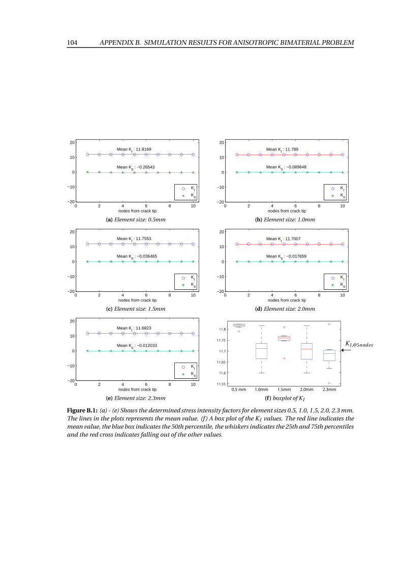
104 APPENDIX B. SIMULATION RESULTS FOR ANISOTROPIC BIMATERIAL PROBLEM
0 2 4 6 8 10−20
−10
0
10
20
nodes from crack tip
Mean KI : 11.8169
Mean KII : −0.26543
KI
KII
(a) Element size: 0.5mm
0 2 4 6 8 10−20
−10
0
10
20
nodes from crack tip
Mean KI : 11.789
Mean KII : −0.089648
KI
KII
(b) Element size: 1.0mm
0 2 4 6 8 10−20
−10
0
10
20
nodes from crack tip
Mean KI : 11.7553
Mean KII : −0.036465
KI
KII
(c) Element size: 1.5mm
0 2 4 6 8 10−20
−10
0
10
20
nodes from crack tip
Mean KI : 11.7007
Mean KII : −0.017659
KI
KII
(d) Element size: 2.0mm
0 2 4 6 8 10−20
−10
0
10
20
nodes from crack tip
Mean KI : 11.6823
Mean KII : −0.012033
KI
KII
(e) Element size: 2.3mm
11.55
11.6
11.65
11.7
11.75
11.8
0.5 mm 1.0mm 1.5mm 2.0mm 2.3mm
K I ,@5nodes
(f ) boxplot of K I
Figure B.1: (a) - (e) Shows the determined stress intensity factors for element sizes 0.5, 1.0, 1.5, 2.0, 2.3 mm.
The lines in the plots represents the mean value. (f ) A box plot of the K I values. The red line indicates the
mean value, the blue box indicates the 50th percentile, the whiskers indicates the 25th and 75th percentiles
and the red cross indicates falling out of the other values.