modeling of piston pin lubrication in internal combustion
TRANSCRIPT

Modeling of Piston Pin Lubrication in Internal Combustion Engines
by
Zhen Meng
B. Eng., Vehicle Engineering Tsinghua University, 2015
S.M., Mechanical Engineering
Massachusetts Institute of Technology, 2017
Submitted to the Department of Mechanical Engineering in Partial Fulfillment of the Requirement for the Degree of
Doctor of Philosophy in Mechanical Engineering and Computation
at the
MASSACHUSETTS INSTITUTE of TECHNOLOGY
September 2020
© 2020 Massachusetts Institute of Technology. All rights reserved.
Signature of Author: _____________________________________________________________ Department of Mechanical Engineering
August 15, 2020
Certified by: _ _________________________________________________________________ Tian Tian
Principal Research Engineer, Department of Mechanical Engineering, MIT Thesis Supervisor
Accepted by: ___________________________________________________________________
Nicolas Hadjiconstantinou Chairman, Department Committee on Graduate Students, MIT
Co-Director, Computational Science and Engineering, MIT


3
Modeling of Piston Pin Lubrication in Internal Combustion Engines
by
Zhen Meng
Submitted to the Department of Mechanical Engineering on August 15, 2020
in Partial Fulfillment of the Requirements of the Degree of
Doctor of Philosophy in Mechanical Engineering and Computation
Abstract
The piston pin joins the piston and the connecting rod to transfer the linear force on the
piston to rotate the crankshaft that is the eventual power outlet of the engine. The interfaces
between the piston pin and the pin bore as well as the connecting rod small end are one of the
most heavily loaded tribo pairs in engines. Piston pin seizure still occurs often in the engine
development and the solution often comes from applying expensive coatings. Furthermore, it
has been found that the friction loss associated with the pin can be a significant contributor to
the total engine mechanical loss. Yet, there lacks a basic understanding of the lubrication
behavior of the pin interfaces.
This work is aimed to develop a piston pin lubrication model with consideration of all
the important mechanical processes. The model predicts the dynamics of the pin and the
lubrication of the interfaces between the pin and pin bore as well as small end. The model
couples the dynamics of the pin with the structural deformation of the mating parts, the
hydrodynamic and boundary lubrication of all the interfaces, and oil transport. The model is
successfully implemented with an efficient and robust numerical solver with the second order
accuracy to compute this highly stiff system. The preliminary results applying the model to a
gasoline engine show that the boundary lubrication is the predominant contributor to the total

4
friction. As a result, the interface with more asperity contact tends to hold the pin with it. Thus,
the pin friction loss is coming from the interface with less contact. Solely from friction reduction
point of view, ensuring efficient hydrodynamics lubrication in one interface is sufficient.
Furthermore, as the heavy load is supported in several small areas, mechanical and thermal
deformation of all the parts are critical to load distribution, oil transport, and the generation of
hydrodynamic and asperity contact pressure, providing the necessity of the elements
integrated in the model.
This work represents the first step to establishing a more comprehensive engineering
model that helps the industry understand the pin lubrication and find cost-effective solutions to
overcome the existing challenges.
Thesis Supervisor: Dr. Tian Tian
Title: Principle Research Engineer, Department of Mechanical Engineering, MIT

5
Acknowledgements
This work was sponsored by Daimler and the Consortium on Lubrication in Internal
Combustion Engines in the Sloan Automotive Laboratory, Massachusetts Institute of
Technology. The consortium members were Mahle, MTU, Shell, Toyota, Volkswagen, Volvo
Trucks, and Weichai Power.
First of all, I would like to express my sincere gratitude for my advisor, Dr. Tian Tian, for
his inspiration and guidance during my time at MIT. He showed and lead me to a higher level of
thinking and working in terms of solving real-world problems as an engineer. He has been not
only the best source for me to seek advice in research, but also a valuable friend as I’ve learned
a lot from his experience and insights of life.
I would also like to thank the other members in my thesis committee, Professor Ton
Lubrecht, Professor Wai Cheng, and Professor Irmgard Bischofberger. They have given me a lot
of advice from various perspectives to help me make my work more comprehensive.
I would like to thank the members of the Sloan Automotive Laboratory at MIT for their
help and exchange of ideas and knowledge. Especially, I’ve been really enjoying the time
working together with fellow students in my group, Yang Liu, Tianshi Fang, Sebastian Ahling,
Chongjie Gu, Qin Zhang, Wang Zhang, Jerome Sacherer, Zhiyuan Shu, and Koji Kikuhara. Special
thanks to Janet Maslow for assisting our research in the lab.
Finally, I would like to thank my parents, Xuemin Zhao and Qiang Meng, and my
girlfriend, Jingru Cao, for everything they’ve done for me.
Zhen Meng, Cambridge, MA, August 2020

6

7
Table of Contents
ABSTRACT ............................................................................................................................................... 3
ACKNOWLEDGEMENTS ........................................................................................................................... 5
LIST OF FIGURES ................................................................................................................................... 11
LIST OF TABLES ..................................................................................................................................... 15
CHAPTER 1 INTRODUCTION .............................................................................................................. 17
1.1 BACKGROUND AND MOTIVATION ...................................................................................................... 17 1.1.1 Power cylinder system .......................................................................................................... 18 1.1.2 Piston pin system .................................................................................................................. 20
1.2 EXISTING WORK ............................................................................................................................. 21 1.3 OBJECTIVES ................................................................................................................................... 23 1.4 THESIS SCOPE ................................................................................................................................ 24
CHAPTER 2 MAJOR FACTORS OF THE MODEL ................................................................................... 26
2.1 KINEMATICS AND DYNAMICS ............................................................................................................. 26 2.1.1 Definitions and simplifications .............................................................................................. 26 2.1.2 System kinematics ................................................................................................................ 27 2.1.3 System dynamics ................................................................................................................... 29
2.2 GEOMETRY OF THE INTERFACES ......................................................................................................... 30 2.2.1 Contours of the interfaces ..................................................................................................... 30 2.2.2 Clearance profile between the surfaces ................................................................................ 32
2.3 ASPERITY CONTACT SUB-MODEL ........................................................................................................ 33 2.4 HYDRODYNAMIC SUB-MODEL ........................................................................................................... 33
2.4.1 Governing equations ............................................................................................................. 33 2.4.2 Boundary conditions ............................................................................................................. 34
2.5 CALCULATION OF FRICTION ............................................................................................................... 35 2.5.1 Calculation of friction power loss .......................................................................................... 35 2.5.2 Friction in boundary lubrication regime ................................................................................ 38 2.5.3 Friction from hydrodynamic shear stress .............................................................................. 39 2.5.4 Summary ............................................................................................................................... 39
2.6 STRUCTURAL DEFORMATION ............................................................................................................. 39 2.7 SUMMARY .................................................................................................................................... 40

8
CHAPTER 3 SOLUTION METHOD ....................................................................................................... 42
3.1 STRUCTURE OF THE SOLVER .............................................................................................................. 42 3.1.1 Main architecture ................................................................................................................. 42 3.1.2 Hydrodynamic module with P-q algorithm ........................................................................... 44
3.2 NUMERICAL SCHEMES ..................................................................................................................... 46 3.2.1 Reynolds equation ................................................................................................................. 46 3.2.2 Equations of system dynamics .............................................................................................. 47
3.3 JACOBIAN MATRIX FOR NEWTON’S METHOD ....................................................................................... 48 3.4 ACCURACY OF THE SCHEMES ............................................................................................................. 51 3.5 SUMMARY .................................................................................................................................... 54
CHAPTER 4 MODEL RESULTS WITH BASIC INPUT ............................................................................... 55
4.1 DYNAMICS OF THE SYSTEM ............................................................................................................... 56 4.1.1 Reciprocation of the piston ................................................................................................... 56 4.1.2 Normal forces on the pin ...................................................................................................... 57 4.1.3 Rotation of the pin ................................................................................................................ 60 4.1.4 Friction force and power loss ................................................................................................ 61
4.2 OIL TRANSPORT PATTERN ................................................................................................................ 64 4.2.1 Intake stroke ......................................................................................................................... 67 4.2.2 Compression stroke ............................................................................................................... 69 4.2.3 Expansion stroke ................................................................................................................... 70 4.2.4 Exhaust stroke ....................................................................................................................... 72 4.2.5 Summary ............................................................................................................................... 73
4.3 PARAMETRIC STUDY ........................................................................................................................ 74 4.3.1 Installation clearance ............................................................................................................ 74
4.3.1.1 Between the pin and the pin boss ................................................................................................... 74 4.3.1.2 Between the pin and the small end bearing .................................................................................... 77
4.3.2 Roughness of the surfaces .................................................................................................... 79 4.3.2.1 Roughness of the pin boss ............................................................................................................... 80 4.3.2.2 Roughness of the small end bearing ............................................................................................... 83
4.3.3 Coefficient of friction ............................................................................................................ 85 4.3.3.1 Coefficient of friction between pin and pin boss ............................................................................ 85 4.3.3.2 Coefficient of friction between pin and small end bearing ............................................................. 89
4.3.4 Engine speed ......................................................................................................................... 92 4.3.5 Cavitation pressure ............................................................................................................... 93
4.4 EFFECTS OF DEFORMATION OF THE PIN ............................................................................................... 95

9
4.5 SUMMARY .................................................................................................................................. 102
CHAPTER 5 APPLICATION TO A MODERN GASOLINE ENGINE .......................................................... 104
5.1 INPUT SETUP ............................................................................................................................... 104 5.2 RESULTS WITH RIGID AND ELASTIC COMPONENTS ............................................................................... 107 5.3 EFFECTS OF DESIGN FEATURES ON THE PIN BOSS ................................................................................ 113
CHAPTER 6 CONCLUSIONS .............................................................................................................. 117
6.1 CONCLUSIONS .............................................................................................................................. 117 6.2 FUTURE WORK ............................................................................................................................ 118
REFERENCES ....................................................................................................................................... 120

10

11
List of Figures
FIGURE 1.1 POWER CYLINDER SYSTEM AND THE MOTIONS OF THE PISTON ................................................................................... 19 FIGURE 1.2 FORCES ON THE PISTON EXCLUDING FRICTION FORCES AT EARLY EXPANSION STROKE ...................................................... 20 FIGURE 1.3 CONNECTION OF PISTON AND CON ROD THROUGH THE PIN ....................................................................................... 21 FIGURE 1.4 EXPANDED VIEW OF THE INTERFACES WITH THE PIN ................................................................................................ 21 FIGURE 2.1 IMPORTANT GEOMETRICAL PARAMETERS OF THE PISTON PIN LUBRICATION MODEL ........................................................ 26 FIGURE 2.2 AXIAL OIL SLOTS ON THE PISTON PIN BOSS AND THE CORRESPONDING INTERFACES ........................................................ 30 FIGURE 2.3 CIRCUMFERENTIAL OIL GROOVES ON THE PISTON PIN BOSS AND THE CORRESPONDING INTERFACES ................................... 31 FIGURE 2.4 FORCES ON THE PISTON, PIN, CON ROD, AND CRANKSHAFT WITHOUT FRICTION ............................................................ 35 FIGURE 2.5 RELATION BETWEEN BOUNDARY FRICTION COEFFICIENT AND RELATIVE VELOCITY ........................................................... 38 FIGURE 3.1 OVERALL STRUCTURE OF THE NUMERICAL SOLVER .................................................................................................. 43 FIGURE 3.2 DIFFERENCE IN THE PRESSURES IN THE MIDDLE OF THE PIN AT PEAK CYLINDER PRESSURE WITH DIFFERENT GRIDS AND FIRST
ORDER ACCURACY SCHEME ....................................................................................................................................... 53 FIGURE 3.3 DIFFERENCE IN THE PRESSURES IN THE MIDDLE OF THE PIN AT PEAK CYLINDER PRESSURE WITH DIFFERENT GRIDS AND SECOND
ORDER ACCURACY SCHEME ....................................................................................................................................... 53 FIGURE 4.1 AXIAL ACCELERATION OF THE PISTON AND PIN IN THE BASELINE CALCULATION .............................................................. 57 FIGURE 4.2 HYDRODYNAMIC NORMAL FORCES ON THE PIN IN THE BASELINE CALCULATION ............................................................. 57 FIGURE 4.3 ASPERITY CONTACT NORMAL FORCES ON THE PIN IN THE BASELINE CALCULATION .......................................................... 58 FIGURE 4.4 MAGNITUDE OF HYDRODYNAMIC AXIAL FORCES ON THE PIN IN THE BASELINE CALCULATION ............................................ 58 FIGURE 4.5 MAGNITUDE OF ASPERITY CONTACT AXIAL FORCES ON THE PIN IN THE BASELINE CALCULATION ........................................ 59 FIGURE 4.6 NET AXIAL FORCE ON THE PIN IN THE BASELINE CALCULATION .................................................................................... 59 FIGURE 4.7 NET ASPERITY CONTACT NORMAL FORCE ON THE PIN IN THE BASELINE CALCULATION ..................................................... 60 FIGURE 4.8 ANGULAR VELOCITIES OF CON ROD AND PIN IN THE BASELINE CALCULATION ................................................................. 61 FIGURE 4.9 FRICTION FORCES ON THE PIN IN THE BASELINE CALCULATION ................................................................................... 62 FIGURE 4.10 NET FRICTION FORCE ON THE PIN IN THE BASELINE CALCULATION ............................................................................. 62 FIGURE 4.11 EFFECTIVE COEFFICIENT OF FRICTION IN BOUNDARY LUBRICATION IN THE BASELINE CALCULATION ................................... 63 FIGURE 4.12 FRICTION POWER LOSS IN THE BASELINE CALCULATION .......................................................................................... 64 FIGURE 4.13 TYPICAL TRACES OF THE PISTON SLIDING VELOCITY AND THE FRICTION FORCE BETWEEN THE PISTON AND THE CYLINDER FROM
THE PISTON SKIRT LUBRICATION MODEL ....................................................................................................................... 64 FIGURE 4.14 DISTRIBUTION OF ASPERITY CONTACT PRESSURE AT 384 CA IN THE BASELINE CALCULATION ......................................... 65 FIGURE 4.15 DISTRIBUTION OF HYDRODYNAMIC PRESSURE AT 384 CA IN THE BASELINE CALCULATION ............................................. 66 FIGURE 4.16 DISTRIBUTION OF VOID RATIO AT 384 CA IN THE BASELINE CALCULATION ................................................................. 66 FIGURE 4.17 DISTRIBUTION OF PRESSURES AND OIL EXCHANGE AT THE BOUNDARIES AT 90 CA IN THE BASELINE CALCULATION .............. 68

12
FIGURE 4.18 DISTRIBUTION OF PRESSURES AND OIL EXCHANGE AT THE BOUNDARIES AT 135 CA IN THE BASELINE CALCULATION ............ 69 FIGURE 4.19 DISTRIBUTION OF PRESSURES AND OIL EXCHANGE AT THE BOUNDARIES AT 315 CA IN THE BASELINE CALCULATION ............ 70 FIGURE 4.20 DISTRIBUTION OF PRESSURES AND OIL EXCHANGE AT THE BOUNDARIES AT 380 CA IN THE BASELINE CALCULATION ............ 71 FIGURE 4.21 CUMULATIVE OIL VOLUME ABSORBED FROM AMBIENT IN THE BASELINE CALCULATION ................................................. 72 FIGURE 4.22 DISTRIBUTION OF PRESSURES AND OIL EXCHANGE AT THE BOUNDARIES AT 675 CA IN THE BASELINE CALCULATION ............ 73 FIGURE 4.23 NORMAL FORCES ON THE PIN WITH DIFFERENT PIN-PIN BOSS INSTALLATION CLEARANCES ............................................. 75 FIGURE 4.24 AVERAGE OIL FILM THICKNESS BETWEEN PIN AND PIN BOSS WITH DIFFERENT PIN-PIN BOSS INSTALLATION CLEARANCES ....... 76 FIGURE 4.25 HYDRODYNAMIC PRESSURE ON A CROSS-SECTION WITH THE SAME BOUNDARY CONDITIONS AND DIFFERENT INSTALLATION
CLEARANCE. .......................................................................................................................................................... 76 FIGURE 4.26 ANGULAR VELOCITIES OF THE PIN WITH DIFFERENT PIN-PIN BOSS INSTALLATION CLEARANCES ........................................ 77 FIGURE 4.27 NORMAL FORCES ON THE PIN WITH DIFFERENT PIN-SMALL END INSTALLATION CLEARANCES .......................................... 78 FIGURE 4.28 ANGULAR VELOCITIES OF THE PIN WITH DIFFERENT PIN-SMALL END INSTALLATION CLEARANCES ..................................... 78 FIGURE 4.29 NORMAL FORCES ON THE PIN WITH DIFFERENT ROUGHNESS ON THE PIN BOSS AND THE SMALL END BEARING .................... 80 FIGURE 4.30 NORMAL FORCES ON THE PIN WITH DIFFERENT PIN BOSS ROUGHNESS ....................................................................... 81 FIGURE 4.31 ANGULAR VELOCITIES OF THE PIN WITH DIFFERENT PIN BOSS ROUGHNESS .................................................................. 82 FIGURE 4.32 FRICTION FORCE BETWEEN THE PIN AND THE SMALL END BEARING WITH DIFFERENT PIN BOSS ROUGHNESS ....................... 82 FIGURE 4.33 FRICTION FORCE BETWEEN THE PIN AND THE PIN BOSS WITH DIFFERENT PIN BOSS ROUGHNESS ...................................... 83 FIGURE 4.34 FRICTION POWER LOSS AND FMEP WITH DIFFERENT PIN BOSS ROUGHNESS ............................................................... 83 FIGURE 4.35 ANGULAR VELOCITIES OF THE PIN WITH DIFFERENT SMALL END BEARING ROUGHNESS .................................................. 84 FIGURE 4.36 NORMAL FORCES ON THE PIN WITH DIFFERENT SMALL END BEARING ROUGHNESS ....................................................... 84 FIGURE 4.37 ANGULAR VELOCITIES OF THE PIN WITH DIFFERENT COEFFICIENT OF FRICTION BETWEEN PIN AND PIN BORE ...................... 85 FIGURE 4.38 NORMAL FORCES ON THE PIN WITH DIFFERENT COEFFICIENT OF FRICTION BETWEEN PIN AND PIN BORE ............................ 86 FIGURE 4.39 SLIDING OIL FLOW RATE INTO THE CRITICAL REGION OF THE SMALL END WITH DIFFERENT COEFFICIENT OF FRICTION BETWEEN
PIN AND PIN BORE ................................................................................................................................................... 86 FIGURE 4.40 PRESSURE DISTRIBUTIONS AND OIL FLOW THROUGH THE BOUNDARIES AT 135 CA WITH DIFFERENT COEFFICIENT OF FRICTION
BETWEEN PIN AND PIN BORE ..................................................................................................................................... 88 FIGURE 4.41 PRESSURE DISTRIBUTIONS AND OIL FLOW THROUGH THE BOUNDARIES AT 315 CA WITH DIFFERENT COEFFICIENT OF FRICTION
BETWEEN PIN AND PIN BORE ..................................................................................................................................... 88 FIGURE 4.42 NORMAL FORCES ON THE PIN WITH DIFFERENT COEFFICIENT OF FRICTION BETWEEN PIN AND SMALL END BEARING ............. 89 FIGURE 4.43 ANGULAR VELOCITIES OF THE PIN WITH DIFFERENT COEFFICIENT OF FRICTION BETWEEN PIN AND SMALL END BEARING ....... 90 FIGURE 4.44 FRICTION FORCE BETWEEN THE PIN AND THE SMALL END BEARING WITH DIFFERENT COEFFICIENT OF FRICTION .................. 91 FIGURE 4.45 EFFECTIVE COEFFICIENT OF FRICTION BETWEEN THE PIN AND THE SMALL END BEARING WITH DIFFERENT SLIDING COEFFICIENT
OF FRICTION .......................................................................................................................................................... 91 FIGURE 4.46 FRICTION POWER LOSS AND FMEP WITH DIFFERENT COEFFICIENT OF FRICTION BETWEEN PIN AND SMALL END BEARING ..... 91 FIGURE 4.47 NORMAL FORCES ON THE PIN WITH DIFFERENT ENGINE SPEEDS ............................................................................... 92

13
FIGURE 4.48 SLIDING OIL FLOW RATE INTO THE CRITICAL REGION OF THE SMALL END WITH DIFFERENT ENGINE SPEEDS ......................... 93 FIGURE 4.49 NORMAL FORCES ON THE PIN WITH DIFFERENT CAVITATION PRESSURES .................................................................... 94 FIGURE 4.50 HYDRODYNAMIC PRESSURE [BAR] AT 380 CA WITH DIFFERENT CAVITATION PRESSURES ............................................... 95 FIGURE 4.51 AVERAGE OIL FILM THICKNESS IN THE CRITICAL REGION OF THE PIN-SMALL END INTERFACE ........................................... 95 FIGURE 4.52 DEFORMATION OF THE PIN WITH TWO 1000N FORCES AT THE ENDS AND A 2000N FORCE IN THE MIDDLE ...................... 96 FIGURE 4.53 NORMAL FORCES ON THE INTERFACES WITH RIGID AND ELASTIC PINS ........................................................................ 97 FIGURE 4.54 ANGULAR VELOCITIES OF RIGID AND ELASTIC PINS ................................................................................................. 97 FIGURE 4.55 CLEARANCE, DEFORMATION, OIL FLOW RATE, AND PRESSURES ON THE INTERFACES AT 120 CA ..................................... 99 FIGURE 4.56 CLEARANCE, DEFORMATION, OIL FLOW RATE, AND PRESSURES ON THE INTERFACES AT 300 CA ................................... 100 FIGURE 4.57 CLEARANCE, DEFORMATION, OIL FLOW RATE, AND PRESSURES ON THE INTERFACES AT 500 CA ................................... 101 FIGURE 4.58 FRICTION POWER LOSS WITH RIGID AND ELASTIC PINS .......................................................................................... 102 FIGURE 5.1 COLD RADIAL VARIANCE (MICROMETER) OF THE PIN .............................................................................................. 105 FIGURE 5.2 ADDITIONAL RADIAL VARIANCE (MICROMETER) OF THE PIN BOSS DUE TO THERMAL LOAD ............................................. 105 FIGURE 5.3 TOTAL RADIAL VARIANCE (MICROMETER) OF THE PIN ............................................................................................ 106 FIGURE 5.4 COMBUSTION PRESSURE TRACE USED IN THE CALCULATION .................................................................................... 106 FIGURE 5.5 NORMAL FORCES ON THE PIN WITH DIFFERENT CONSIDERATIONS OF DEFORMATION .................................................... 107 FIGURE 5.6 FRICTION FORCE BETWEEN THE PIN AND THE PIN BOSS WITH DIFFERENT CONSIDERATIONS OF DEFORMATION ................... 108 FIGURE 5.7 FRICTION POWER LOSS AND FMEP BETWEEN THE PIN AND THE SMALL END WITH DIFFERENT CONSIDERATIONS OF
DEFORMATION ..................................................................................................................................................... 108 FIGURE 5.8 ANGULAR VELOCITY OF THE PIN WITH DIFFERENT CONSIDERATIONS OF DEFORMATION ................................................. 109 FIGURE 5.9 ASPERITY CONTACT PRESSURE [BAR] AT 385 CA IN THE RIGID CASE ......................................................................... 109 FIGURE 5.10 HYDRODYNAMIC PRESSURE [BAR] AT 385 CA IN THE RIGID CASE ........................................................................... 110 FIGURE 5.11 MAGNIFIED DEFORMATION [𝝁M] OF THE PIN AT 385 CA IN THE CASE WITH ELASTIC PIN ........................................... 110 FIGURE 5.12 CLEARANCE BETWEEN PIN AND SMALL END AT 385 CA ....................................................................................... 111 FIGURE 5.13 ASPERITY CONTACT PRESSURE [BAR] AT 385 CA IN THE CASE WITH ELASTIC PIN ....................................................... 111 FIGURE 5.14 HYDRODYNAMIC PRESSURE [BAR] AT 385 CA IN THE CASE WITH ELASTIC PIN ........................................................... 111 FIGURE 5.15 MAGNIFIED DEFORMATION [𝝁M] OF THE PIN BOSS AT 385 CA IN THE CASE WITH ELASTIC PIN AND PIN BOSS ................. 112 FIGURE 5.16 HYDRODYNAMIC PRESSURE [BAR] AT 385 CA IN THE CASE WITH ELASTIC PIN AND PIN BOSS ....................................... 112 FIGURE 5.17 NORMAL FORCES ON THE PIN WITH DIFFERENT PIN BOSS DESIGNS .......................................................................... 114 FIGURE 5.18 ANGULAR VELOCITY OF THE PIN WITH DIFFERENT PIN BOSS DESIGNS ....................................................................... 115 FIGURE 5.19 HYDRODYNAMIC PRESSURE DISTRIBUTION AT 340 CA WITH DIFFERENT PIN BOSS DESIGNS ......................................... 115 FIGURE 5.20 FRICTION FORCE BETWEEN PIN AND PIN BOSS AND FMEP WITH DIFFERENT PIN BOSS DESIGNS .................................... 116

14

15
List of Tables TABLE 3.1 MAJOR PARAMETERS FOR TESTING THE ACCURACY OF THE NUMERICAL SCHEMES ........................................................... 52 TABLE 4.1 ENGINE SPECIFICATION OF THE BASELINE CALCULATION ............................................................................................. 55 TABLE 4.2 OTHER IMPORTANT PARAMETERS IN THE BASELINE CALCULATION ................................................................................ 55 TABLE 5.1 SPECIFICATION AND RUNNING CONDITION OF THE GASOLINE ENGINE STUDIED IN SECTION 5.1 ........................................ 104

16

17
Chapter 1 Introduction
1.1 Background and Motivation
Internal combustion engines have been widely used in the propulsion systems of
automotive vehicles and are expected to keep their predominance in the market in the
following decades [1]. Yet, continuous increase of the consumption of motor fuels with the
expansion of the car ownership has imposed to the world a significant challenge in terms of
environmental disruption and resource depletion. In order to address this challenge, extensive
effort has been made to improve the efficiency of the engines.
The energy loss due to the friction in the piston assembly is estimated to account for
15% of the total loss in typical engines [2], and 55-72% of it can be attributed to the piston and
the connecting rod (con rod) [3]. As the connection between these two components, the piston
pin is crucial to the performance of the entire engine.
Because of the limited surface area, the pressure taken by the pin during engine
operation can attain 100 MPa, and a large proportion of it is supported by boundary
lubrication. As a result, the pin still experiences severe wear and sometimes seizure in the
development of modern engines. Quiet often, standard protocols to change the mechanical and
geometrical designs of the pin fail to resolve the issue and costly DLC coating has to be applied.
In an experimental study on the Friction Mean Effective Pressure (FMEP) of a turbo-
charged gasoline engine, it was observed that modifications to the piston pin boss, such as axial
oil slots, circumferential oil grooves, and larger diameters, are able to reduce the FMEP
significantly [4]. However, the exact mechanisms contributing to the observed friction change
are largely unclear although the evidences suggested that the amount of oil lubricating the
pin/pin-bore interface may play a critical role in pin friction. Therefore, an adequate analytical
tool is needed in the industry to help develop new designs systematically and cost-effectively.
While maximizing the hydrodynamic pressure generation and minimizing direct asperity
contact are the goal to reduce wear, friction, and risk for seizure, there is limited understanding
how the lubricant outside of the interfaces of the pin and its mating parts interacts with the

18
primary and secondary motion of the pin, and how oil is transported to the area bearing the
thrust force. Furthermore, the lubrication depends highly on the rotation of the pin, the
geometry of the pin and the bearings, the structural deformation of the components, and the
surface roughness. On the other hand, the rotation of the pin is also dependent on the
lubrication. This introduces a unique challenge for modeling the pin lubrication problem, as the
primary motion of the system needs to be predicted as well. In addition, although the
interfaces, namely, pin and piston and pin and con rod, are completely separated geometrically,
they are affecting each other through their influence on the rotation of the pin.
1.1.1 Power cylinder system
Figure 1.1 shows the main components of the power cylinder system in a four-stroke
internal combustion engine at early expansion stroke, when the combustion of the fuel
generates enormous pressure in the combustion chamber and pushes the piston to move
downwards. Guided by the cylinder liner, the primary motion of the piston is the reciprocation
along the axial direction. This motion is transferred to the rotation of the crankshaft through
the piston pin and the connecting rod.
Due to the gap between the piston and the liner, which is usually in the order of 10
micrometers, the piston also translates in the lateral direction and tilts around the pin. The
lateral motion and tilting are referred to as the piston secondary motion.
Figure 1.2 shows the forces acting on the piston from other components with the
friction neglected. In the axial direction, the force from the pin is balancing the pressure from
the combustion chamber. In the lateral direction, it balances the forces from the liner. Both the
forces from the pin and the liner are contributed by hydrodynamic pressure and solid-solid
contact pressure.
Bai [5], Totaro [6], and Zhen [7-9] developed successively a comprehensive model to
study the interaction between the piston and the liner. The model integrates the dynamics of
the components, structural deformation, friction generation on the interface, lubrication and
oil transport between the piston skirt and the liner, and the breaking-in of the piston-skirt

19
surfaces. The model is also able to calculate the piston secondary motion, which will be directly
associated with this study.
Figure 1.1 Power cylinder system and the motions of the piston

20
Figure 1.2 Forces on the piston excluding friction forces at early expansion stroke
1.1.2 Piston pin system
Figure 1.3 [10] shows how the piston pin is installed inside the piston and the con rod.
The directions of the axes are the same as in Figure 1.1. In most of the modern engines, the pin
has a fully floating configuration where it is able to rotate around its axis (𝑦). The rotation will
be referred to as the primary motion of the pin.
The pin has a basic shape of a hollow cylinder, with the outer diameter more than one
tenth of the length. Therefore, in the expanded view of its side surface, as shown in Figure 1.4,
the length in both axial and circumferential directions have the same order of magnitude of 10s
of millimeters. The interface between the pin and the con-rod small-end is in the center,
whereas the interfaces between the pin and the piston pin boss are on the two ends.
Although the centers of the pin, the con rod small end, and the piston pin boss are
overlapping at 𝑃 in Figure 1.3, their locations will be different because of the clearance among
the components, which are usually in the order of 10 micrometers. The relative movement will
be referred to as the secondary motion of the system.
The secondary motion will determine the interaction on the interfaces, such as the
generation of hydrodynamic pressure and asperity contact pressure. The distribution of the
pressures, in turn, will affect the dynamics. This makes it more challenging to simulate the
system.

21
Figure 1.3 Connection of piston and con rod through the pin
Figure 1.4 Expanded view of the interfaces with the pin
1.2 Existing Work
There have been both experimental and computational studies on the piston pin
system. In 1997, Suhara et al. [11] designed an original device to measure the friction on the
piston pin boss bearing from the phase difference between the rotational oscillations of the
bearing and the semi-floating pin. Although the oscillation signals were affected by the

22
intermediate spring, the device was able to help generalize the pattern of friction during an
engine cycle and study the effects of different design parameters. Iwasaki et al. [12] developed
a measurement device for a gasoline engine that collected bending stress of the pin as the
friction on the small end bearing. It was found that at higher engine speeds, the edges of the
bearing would experience severe asperity contact, which can be alleviated with the addition of
side relief to the bearing. The device was also able to measure the secondary motion of the pin,
showing that the pin would stay with the upper side of the small end bearing during most of the
engine cycle.
Clark et al. [13] tested the dynamics of the floating piston pin in a diesel engine and
identified the outer edges of the small end and the inner edges of piston pin bore as the places
with highest dry contact. Pin rotation was also measured and was shown to have a clockwise
cumulative rotation angle as defined in Figure 1.1. Abed et al [14] developed a motion data
acquisition system to capture the rotation angle of the pin against the piston pin bore, and
received a similar pattern in terms of net rotation.
Miura et al. [15] used thin-film sensors to measure the oil pressure in the fully flooded
interface between the pin and the piston pin boss. It was found that the highest hydrodynamic
pressure occurs near the inner edges of the pin boss and around 𝜑 = ±45° in the
circumference as shown in Figure 1.3.
On the modeling side, Ligier and Ragot [16] developed a simple hydrodynamic
lubrication program with a refined contact model to simulate the general behavior of the piston
pin, including the motion and the wear. The surface of the pin is assumed to be fully flooded
with lubricating oil, and the load carrying capacity is provided only by the squeeze of the oil.
Fridman, Piraner, and Clark [17] developed a model for the pin in heavy-duty diesel
engines. The results showed that the pin would slightly rotate in the direction of the crankshaft
rotation, which is consistent with the experimental results discussed above. It also showed a
contact pressure distribution that is similar to the wear pattern observed in the pin bushing.
The model does not include the structural deformation of the bearings.
Wang et al. [18] carried out an EHD lubrication analysis between the pin and the small
end bush, assuming the clearance is entirely filled with lubricant. Bertocchi, Giacopini, and Dini

23
[19] developed an algorithm to study the small end and big end based on the complementarity
relation between the hydrodynamic pressure and void fraction of the clearance of the
interfaces to guarantee the conservation of mass while considering cavitation. However, the
components are simplified as rigid.
Shi [20] designed a more comprehensive analytical model for the floating piston pin that
coupled the pin rotation, elastic deformation, lubrication, cavitation, and asperity contact. It
showed that the contact pressure became more concentrated with the deflection of the pin,
which can be improved with higher stiffness. Because the model calculates the rotation of the
pin with explicit time-marching integration, some of the results are unstable and oscillating
during the expansion stroke of the engine.
Ba et al. [21] built a multi-body dynamic model to analyze the lubrication for the piston
pin joint. It mainly consisted of an EHD solver that included film cavitation and asperity contact.
Different modifications to the geometries of the pin bore were tested to provide guidance for
the design. The structural deformation of the pin is simplified as bending deflection, whereas
the deformation of the pin boss is calculated from structural analysis rather than implicitly
computed in the model.
1.3 Objectives
The existing models for piston pin lubrication have at least one of the following
simplifications
• The interfaces between the pin and its mating part are fully filled with lubricant.
• The engine components are rigid.
• The engine components are not rigid, but their mechanical deformation is pre-
determined.
• Asperity contact pressure is not considered.
• The rotation of the pin is calculated explicitly.
The main objective of this study is to develop a comprehensive piston pin lubrication
model that has the following features

24
• To integrate the major processes critical to the lubrication of the pin, including
primary (pin rotation) and secondary motion of the pin, structural deformation of
the components, oil transport at the interfaces, hydrodynamic lubrication with mass
conservation between full and partial film regions, asperity contact and friction of
boundary lubrication considering stick and slip of the pin with its interfaces.
• To couple the two interfaces, which are indirectly affecting each other as both the
small end and the pin boss have forces on the pin.
• To apply an implicit numerical scheme that solves the system with robustness and
efficiency. The system is not only highly non-linear, but also very stiff as the net
force/inertia force of the pin is much smaller than the forces at each interface.
• To establish a relation among the major factors and understand how the system
works.
1.4 Thesis Scope
The second chapter introduces the major mechanical processes considered in the
model. It identifies the degrees of freedom in the system dynamics, as well as the equations
regarding their equilibrium. It also specifies the other unknowns and the related correlations,
including the geometry of the interfaces, the hydrodynamic and asperity contact pressures,
generation of friction force, and structural deformation.
The third chapter discusses the solution method of the system. It first introduces the
overall structure of the solver, including the algorithm in the hydrodynamic module that
incorporates full film and partial film regions while guaranteeing mass conservation. It also
explains the finite difference scheme with second-order accuracy to discretize the equations for
the Jacobian matrix of the Newton’s method.
The fourth chapter shows the results of the model with input data derived from a turbo-
charged gasoline engine. It starts with analyzing the general patterns of the dynamics and oil
transport during the engine cycle, followed by the parametric study on the installation
clearance, roughness, coefficient of friction, and engine speed. Finally, the effects of the
structural deformation of the pin is investigated.

25
The fifth chapter discusses the application of the model to a modern gasoline engine
with the profile and structural deformation of the pin boss considered.
The last chapter summarizes the thesis work with conclusions and remarks and suggests
several aspects on this topic to investigate in this future.

26
Chapter 2 Major Factors of the Model
2.1 Kinematics and Dynamics
2.1.1 Definitions and simplifications
Figure 2.1 shows some important geometrical parameters involved in the model. As
explained in the first chapter, the centers of the pin (𝑃), the con rod small end (𝑃!), and the
piston pin boss (𝑃") are three different points, and the relative locations among them are
critical to the system. 𝑄 denotes the center of the con rod big end and 𝐶 denotes the center of
gravity of the con rod. The center of the crank shaft (𝑂) is defined as the origin of the
coordinate system.
Figure 2.1 Important geometrical parameters of the piston pin lubrication model

27
The model has a few simplifications regarding the kinematics and dynamics. First, the
angular velocity of the crank shaft, �̇�, is assumed to be constant throughout the entire engine
cycle.
The forces between the con rod big end and the crank shaft are neglected when
calculating the torque equilibrium of the con rod around the big end because of their limited
arms compared to the forces at the small end.
Finally, the friction forces between the pin and the pin boss and between the pin and
the small end are neglected in the equations of force balance as their magnitudes are much
smaller than the normal forces.
2.1.2 System kinematics
There are five degrees of freedom in the system. The first three are the location of the
pin in the lateral (𝑥) and axial (𝑧) directions and the rotation of the pin along the 𝑦 axis, which
are denoted by 𝑥#, 𝑧#, and 𝛼#. The fourth degree of freedom is the rotation of the con rod, 𝛼#!.
Both 𝛼# and 𝛼#! are defined as positive when they are clockwise from the opposite direction of
𝑧 (𝛼#! is negative in Figure 2.1). The last degree of freedom is the axial location of the piston pin
boss, 𝑧#".
The locations of 𝑃! are dependent on 𝛼#!, whereas the lateral location of 𝑃" can be
imported from the result of the piston skirt lubrication model [5]. This input can be substituted
with no secondary motion if the secondary motion is not available and the results should not
have appreciable difference with the ones with secondary motion provided.
In the model, every time step is represented by the angle 𝛽 of the crankshaft, defined as
clockwise from 𝑧 axis. With 𝛽 known, the location, velocity, and acceleration of the con rod big
end are
𝑥$ = −𝑟% sin 𝛽 (2.1)
𝑧$ = 𝑟% cos 𝛽 (2.2)

28
�̇�$ = −𝑟%𝜔 cos 𝛽 (2.3)
�̇�$ = −𝑟%𝜔 sin 𝛽 (2.4)
�̈�$ = 𝑟%𝜔" sin 𝛽 (2.5)
�̈�$ = −𝑟%𝜔" cos 𝛽 (2.6)
Here 𝑟% is the radius of the crankshaft, which is the fixed distance between 𝑂 and 𝑄.
𝜔 = �̇� is the constant angular velocity of the crankshaft.
The movement of the center of the small end is
𝑥#! = −𝑟% sin 𝛽 − 𝑙! sin 𝛼#! (2.7)
𝑧#! = 𝑟% cos 𝛽 + 𝑙! cos 𝛼#! (2.8)
�̇�#! = −𝑟%𝜔 cos 𝛽 − 𝑙!�̇�#! cos 𝛼#! (2.9)
�̇�#! = −𝑟%𝜔 sin 𝛽 − 𝑙!�̇�#! sin 𝛼#! (2.10)
�̈�#! = 𝑟%𝜔" sin 𝛽 + 𝑙!H�̇�#!I" sin 𝛼#! − 𝑙!�̈�#! cos 𝛼#! (2.11)
�̈�#! = −𝑟%𝜔" cos 𝛽 − 𝑙!H�̇�#!I" cos 𝛼#! − 𝑙!�̈�#! sin 𝛼#! (2.12)
where 𝑙! is the distance between the centers of the small end and the big end.
The distance of the con rod’s center of gravity from the big end is
𝑥&/$ = 𝑥&( cos 𝛼#! − 𝑧&( sin 𝛼#! (2.13)
𝑧&/$ = 𝑥&( sin 𝛼#! + 𝑧&( cos 𝛼#! (2.14)
with 𝑥&( and 𝑧&( the original distance when the con rod is vertical.
Therefore, the motion of 𝐶 can be derived through the motion of 𝑄
𝑥& = 𝑥&/$ + 𝑥&/$ (2.15)

29
𝑧& = 𝑧$ + 𝑧&/$ (2.16)
�̈�& = �̈�$ − H�̇�#!I"𝑥&/$ − �̈�#!𝑧&/$ (2.17)
�̈�& = �̈�$ − H�̇�#!I"𝑧&/$ + �̈�#!𝑥&/$ (2.18)
2.1.3 System dynamics
Each degree of freedom can be described by an equilibrium equation. For the pin, it
takes a distributed force from the small end bearing and another from the piston pin boss, both
of which can be decomposed into the lateral direction and the axial direction. Therefore, the
force balance for the pin is
𝐹)*"+,- − 𝐹+,-"+ −𝑚�̈�# = 0 (2.19)
𝑁)*"+,- − 𝑁+,-"+ −𝑚�̈�# = 0 (2.20)
Here, 𝑚 is the mass of the pin, 𝐹+,-"+ and 𝑁+,-"+ are the lateral and axial forces from
the pin to the piston, and 𝐹)*"+,- and 𝑁)*"+,- are the forces from the con rod to the pin. The
forces are the summation of hydrodynamic and asperity contact pressures projected to the
corresponding directions.
The torque on the pin comes from the friction forces, and determines the angular
acceleration of the pin
𝑓𝑟 − 𝐼�̈�# = 0 (2.21)
Here, 𝑟 is the radius of the pin, 𝐼 is the moment of inertia around its center of gravity.
The net friction force 𝑓 on the pin will be analyzed in detail in the following subsections.
The equilibrium of torques of the con rod around its big end is
𝑚!H�̈�&𝑧&/$ − �̈�&𝑥&/$I + 𝑙!H𝐹)*"+,- cos 𝛼#! + 𝑁)*"+,- sin 𝛼#!I − 𝐼!,/�̈�#! = 0 (2.22)

30
Here, 𝑚! is the mass of the con rod. 𝐼!,/ is the moment of inertia around 𝑄. The first
term on the left-hand side of the equation is the contribution from the inertia, and the second
term comes from the forces at the small end.
Finally, the axial forces on the piston, including the force from the pin and the
combustion force, are balanced in the 𝑧 direction
𝑁+,-"+ − 𝜋𝑟""𝑝)01/ −𝑚"�̈�#" = 0 (2.23)
𝑟" and 𝑚" are the radius and mass of the piston, 𝑝)01/ is the gauge pressure in the
combustion chamber.
2.2 Geometry of the Interfaces
2.2.1 Contours of the interfaces
As shown in Figure 1.4, in a typical pin system, the side surface of the pin can be divided
into 5 sections: the two interfaces between the pin and the pin boss at the two ends of the pin,
the interface between the pin and the small end in the middle, and two areas in ambient
separating the interfaces.
In some other designs, however, the surface will be more complicated. For example,
when there are oil slots along the axial direction or oil grooves in the circumference of the pin
boss, the interfaces will be further divided if the features are considered as boundary, as shown
in Figures 2.2 and 2.3 [4].
Figure 2.2 Axial oil slots on the piston pin boss and the corresponding interfaces

31
Figure 2.3 Circumferential oil grooves on the piston pin boss and the corresponding interfaces
It is important to identify accurately the contours of each section of the interface and
the ambient areas for arbitrary designs of the components. The first main reason is that the
interpolation of clearance needs to be performed within the same section. In addition, the
ambient areas should not have any asperity contact pressure or more hydrodynamic pressure
than atmospheric.
In order to assign the nodes to correct sections, the model performs a simple cluster
analysis. Suppose that there are 𝑛 nodes in total, the algorithm works as follows
• Assign node 1 to section 1.
• If the distance from node 2 to node 1 is smaller than a threshold, assign node 2
to section 1. Otherwise, assign it to a new section 2.
• For each new node 𝑖, use 𝒢 to denote the set of previous nodes whose distances
from 𝑖 are smaller than the threshold.
o If 𝒢 is empty, assign node 𝑖 to a new section.
o If all the nodes in 𝒢 are in the same section 𝑗, assign 𝑖 to this section.
o If the nodes in 𝒢 are from more than one sections 𝑗!, … , 𝑗2, assign node 𝑖
as well as all the nodes in sections 𝑗", … , 𝑗2 to section 𝑗!.

32
2.2.2 Clearance profile between the surfaces
The base shape of the outer surface of the pin, as well as the inner surfaces of the small
end and pin boss, are cylindrical with constant nominal radii. The difference between the
nominal radii of the mating surfaces is named installation clearance and determines the initial
clearance between the components.
According to the exact design of the bearings in the pin boss and small end, the local
radius might be different from the nominal one. In addition, thermal load also alters the shapes
of the surfaces. Since the effects on the clearance by the installation clearance, designed
profile, and thermal load are not changing within an engine cycle, they will be treated as input
to the model and denoted by ℎ(.
Next, the relative locations among 𝑃, 𝑃!, and 𝑃" will affect the geometry of the
interfaces. As their influence changes with crank angle, they will be part of the solution. As a
result, the clearance between the pin and the small end becomes
ℎ! = ℎ( + H𝑧#! − 𝑧#I cosH𝜑 − 𝛼#!I + H𝑥#! − 𝑥#I sinH𝜑 − 𝛼#!I (2.24)
where 𝜑 is the circumferential location on the side surface of the pin, as shown in Figures 1.3
and 1.4.
The clearance between the pin and the pin boss becomes
ℎ" = ℎ( + H𝑧#" − 𝑧#I cos𝜑 + H𝑥#" − 𝑥#I sin𝜑 (2.25)
Finally, the structural deformation of the surfaces, 𝑑, contributes directly to the
geometry. The final clearance profile in the model is a function of motion and deformation.
ℎ = ℎ( + 𝑓3(𝜉) + 𝑑 (2.26)
Here 𝜉 represents the collection of the five degrees of freedom,𝑓3(𝜉) refers to the
relations in equations 2.24 and 2.25.

33
2.3 Asperity Contact Sub-model
The formula developed by Hu et al. [22] based on the Greenwood-Tripp model [23] is
applied to calculate the asperity contact pressure. If the roughness of the pin and the small end
are 𝜎 and 𝜎!, the effective roughness of their interface will be [24]
𝜎!,455 = [𝜎" + 𝜎!" (2.27)
When the clearance between them is smaller than 4 times of the effective roughness,
asperity contact pressure will arise with a magnitude of
𝑝6 = 𝑐! ]4 −ℎ
𝜎!,455^6"
∙ 𝕀3789!,$%% (2.28)
𝑐! and 𝑐" are constant parameters derived from the material properties. 𝕀 is the
Boolean variable indicating whether or not ℎ is lower than 4𝜎455.
Therefore, the asperity contact is only a function of the clearance and does not need to
be treated as an independent variable in the system.
2.4 Hydrodynamic Sub-model
2.4.1 Governing equations
As the clearances of the interfaces are in the order of 10s of micrometers, which is much
smaller than the length and width, it suffices to use the Reynolds equation to describe the flow
of the lubricating oil.
In order to consider the partial film regions, where there is not enough oil to fill the
entire clearance, the present model applies the algorithm designed by Biboulet and Lubrecht
[25] to guarantee mass conservation. In addition to the hydrodynamic pressure 𝑝, a void
fraction 𝜃 is defined as the ratio between the volume of air and the total volume of the local
cell in the finite difference mesh. Thus, the effective oil film thickness is (1 − 𝜃)ℎ, and the

34
original Reynolds equation that only applies to full film region is generalized to the following
form with constant oil density and dynamic viscosity 𝜂
𝜕𝑟"𝜕𝜑
]ℎ:
12𝜂𝜕𝑝𝜕𝜑^ +
𝜕𝜕𝑦]ℎ:
12𝜂𝜕𝑝𝜕𝑦^ =
𝑢2𝜕(ℎ − 𝜃ℎ)𝑟𝜕𝜑
+𝜕(ℎ − 𝜃ℎ)
𝜕𝑡(2.29)
In the full film regions, where the entire clearance is filled with oil and 𝜃 = 0, the
hydrodynamic pressure will be positive. In the partial film regions, where 𝜃 is larger than 0,
there will be no hydrodynamic pressure. Thus, there exists a complementarity relation between
𝑝 and 𝜃
f𝑝 ≥ 0𝜃 ≥ 0𝑝 ∙ 𝜃 = 0
(2.30)
which is equivalent to
𝑝 + 𝜃 − h𝑝" + 𝜃" = 0 (2.31)
The Reynolds equation and the complementarity equation will be associated with 𝑝 and
𝜃 in the system equations.
2.4.2 Boundary conditions
In addition to the distribution and transport of lubricating oil within the interfaces, there
will be oil exchange with the ambient through the boundaries of the interface. The boundary
conditions for the film thickness and pressure of the oil, therefore, have direct impact on the
lubrication condition of the system. Since related measurement data are hardly available, it is
necessary to make reasonable assumptions regarding the boundary conditions.
The baseline setup of the model assumes that the boundary is filled with lubricant at
ambient pressure. This represents an upper limit of the natural oil supply to the system.
The partial film regions on the interfaces are assumed to be at a constant cavitation
pressure that is lower than ambient. Thus, oil will be absorbed into the interface if the area
near the boundary is not fully flooded.

35
2.5 Calculation of Friction
2.5.1 Calculation of friction power loss
Unlike the calculation of the friction power loss between the piston skirt and the
cylinder liner, which is simply the multiplication of the friction force on the interface and the
sliding velocity of the piston, the power loss associated with the pin is not as straightforward.
Figure 2.4 shows the forces on the components of the piston assembly. Note that 𝛼#!
here is negative. In order to calculate the power loss, the power output to the crankshaft
without any friction is needed. The torque exerted on the crankshaft is
𝑇( = 𝐹);𝑟% cos 𝛽 + 𝑁);𝑟% sin β (2.32)
Figure 2.4 Forces on the piston, pin, con rod, and crankshaft without friction

36
The force on the piston from the combustion chamber is the driving force of the system.
Its magnitude is
𝑁)01/ = 𝜋𝑟""𝑝)01/ (2.33)
The difference between𝑁)01/ and 𝑁);, the axial force from the crankshaft to the con
rod big end, provides the acceleration of the pin, the con rod, and the piston
𝑁); = 𝑁)01/ +𝑚�̈�# +𝑚!�̈�& +𝑚"�̈�#" (2.34)
In order to get an expression for 𝐹); that does not contain any other forces except for
𝑁);, the torque balance of the con rod needs to be based on the center of the small end, 𝑃!
𝑚!H�̈�&𝑧&/#! − �̈�&𝑥&/#!I + 𝑙!H𝐹); cos 𝛼#! + 𝑁); sin 𝛼#!I − 𝐼!,;�̈�#! = 0 (2.35)
Here 𝑥&/#! and 𝑧&/#! are the relative location between the center of gravity of the con
rod and 𝑃!, which is only a function of 𝛼#!. 𝐼!,; is the moment of inertia around 𝑃!.
Therefore,
𝐹); =𝐼!,;�̈�#! +𝑚!H�̈�&𝑥&/#! − �̈�&𝑧&/#!I
𝑙! cos 𝛼#!− 𝑁); tan 𝛼#! (2.36)
The torque output with frictionless condition is
𝑇( =𝑟%
cos 𝛼#!m𝐼!,;�̈�#! +𝑚!H�̈�&𝑥&/#! − �̈�&𝑧&/#!I
𝑙!cos 𝛽 + n𝑁)01/ +o𝑚�̈�p sinH𝛽 − 𝛼#!Iq (2.37)
As the rotational speed of the crankshaft is assumed to be constant, the primary motion
of the piston is almost fixed. Therefore, even if there is friction on the interfaces, the force
balance in the axial direction will be the same as equation (2.34) because the friction forces can
be viewed as internal forces and will cancel off each other. This means that 𝑁); will be the same
as well.
The torque balance of the con rod around 𝑃! will become

37
𝑚!H�̈�&𝑧&/#! − �̈�&𝑥&/#!I + 𝑙!H𝐹); cos 𝛼#! + 𝑁); sin 𝛼#!I − 𝐼!,;�̈�#! − 𝑓!𝑟! = 0 (2.38)
with 𝑓! being the total friction force between the pin and the small end and 𝑟! the radius of the
small end bearing.
Therefore,
𝐹); =𝐼!,;�̈�#! +𝑚!H�̈�&𝑥&/#! − �̈�&𝑧&/#!I + 𝑓!𝑟!
𝑙! cos 𝛼#!− 𝑁); tan 𝛼#! (2.36)
The torque output will decrease from 𝑇( by
∆𝑇 = ∆𝐹);𝑟% cos 𝛽 =𝑟!𝑟% cos 𝛽𝑙! cos 𝛼#!
𝑓! (2.37)
The power output is the multiplication of the torque and the angular velocity of the
crankshaft
∆𝒫 = �̇�∆𝑇 (2.38)
Neglecting the secondary motion of the pin, the rotation of the con rod and crankshaft
can be related as
𝑙! sin 𝛼#! = 𝑟% sin 𝛽 (2.39)
𝑙!�̇�#! cos 𝛼#! = 𝑟%�̇� cos 𝛽 (2.40)
From equations (2.37), (2.38), and (2.40), the final friction power loss is
∆𝒫 = 𝑟!𝑓!�̇�#! (2.41)
This indicates that the friction between the pin and the piston pin boss does not directly
generate loss of power. However, as the interfaces are integrated by the rotation of the pin, the
friction will alter the behavior of the pin/small end interface. Detailed analysis will be provided
in the following chapters.

38
2.5.2 Friction in boundary lubrication regime
In the pin system, if the friction force from the small end bearing is larger than the
friction force from the pin boss, the pin will tend to follow the rotation of the con rod and
rotate against the pin boss. Otherwise, the pin will stay with the pin boss and have relative
sliding with the small end. The stick-slip model [26-27], where the coefficient of friction for
boundary lubrication changes with the sliding velocity, is suitable to describe this process.
However, the function for the coefficient is not always differentiable, which can compromise
the robustness of numerical solver.
The model uses an approximation to the stick-slip model to determine the coefficient of
friction. The coefficient between the pin and the small end bearing is
𝜇! = 𝜇!,( m1 −2
1 + 𝑒2<=̇&!?@̇Aq (2.42)
Here 𝜇!,( is the reference coefficient when the sliding velocity is large enough, 𝑘 is a
pre-determined parameter that alters the shape of the curve.
The coefficient between the pin and the pin boss is
𝜇" = 𝜇",( w1 −2
1 + 𝑒2=̇&!x (2.43)
Figure 2.5 shows the curves with different values of 𝑘.
Figure 2.5 Relation between boundary friction coefficient and relative velocity

39
2.5.3 Friction from hydrodynamic shear stress
The total drag on the pin from the hydrodynamic effects is equivalent to the shear stress
on the bearings.
𝜏 = −𝜂𝑢ℎ+ℎ2𝜕𝑝𝑟𝜕𝜑
(2.44)
Here 𝑢 is sliding velocity of the interface.
2.5.4 Summary
The total friction forces on the interface of the pin and the small end bearing (𝑆!) and
the interface between the pin and pin boss (𝑆") are
𝑓! = 𝜇!,( m1 −2
1 + 𝑒2<=̇&!?@̇Aq ∙o𝑝6
B!
+om−𝜂𝑟H�̇�#! − �̇�I
ℎ +ℎ2𝜕𝑝𝑟𝜕𝜑
qB!
(2.45)
𝑓" = 𝜇",( w1 −2
1 + 𝑒2=̇&!x ∙o𝑝6
B"
+ow−𝜂𝑟�̇�#!ℎ
+ℎ2𝜕𝑝𝑟𝜕𝜑
xB"
(2.46)
They are functions of the motion 𝜉, clearance ℎ, and hydrodynamic pressure 𝑝.
2.6 Structural Deformation
The components will deform accordingly as they are loaded with hydrodynamic and
asperity contact pressures. In the model, elastic deformation will be considered with a linear
relation with the pressure distribution.
𝑑 = 𝑀)01+ ∙ (𝑝 + 𝑝6) (2.47)
Here 𝑀)01+ is the sum of compliance matrices of the components in contact. It will be
calculated prior to the model calculation as an input. 𝑑, 𝑝, and 𝑝6 are vectors with the number
of cells in the mesh as their length.
As the hydrodynamic module requires the size of the cells in the mesh to be small to get
accurate pressure distributions, the structural deformation is generally smoother. On the other

40
hand, while the other parts of the Jacobian matrix are very sparse, the compliance matrix is
dense and will take up considerable computation time.
In order to reduce the size of the compliance matrix so that the calculation can be more
efficient and less memory consuming, two different sets of meshes are defined on the pin. The
calculation of hydrodynamic pressure and clearance is performed on the fine mesh, whereas
the deformation is calculated on the coarse mesh. Since it is straightforward to get the matrices
that interpolate and transform the variables between the meshes, the final form of the
deformation is
𝑑 = 𝑀)"5 ∙ 𝑀)01+ ∙ [𝑀5")(𝑝 + 𝑝6)] (2.48)
Suppose that there are 𝑛5 cells in the fine mesh and 𝑛) cells in the coarse mesh, 𝑀5")
will be a matrix with size 𝑛) × 𝑛5 that transforms the pressures to the coarse mesh, 𝑀)"5 will be
a matrix with size 𝑛5 × 𝑛) that transforms the deformation back to the fine mesh.
2.7 Summary
The pin lubrication model developed in this study integrates most of the important
features in the pin system. The dynamics of the engine components are calculated, including
the rotation of the pin.
To calculate the clearance profile of the interfaces, the model considers the fixed
geometry due to thermal load, the effects of the secondary motions among the components,
and the contribution from the structural deformation.
The model considers the effects of roughness on the asperity contact pressure.
Although the roughness is not included in the calculation of hydrodynamic pressure, the
lubrication part of the model incorporates both full film and partial film regions while
guaranteeing mass conservation of oil.
In the boundary lubrication regime, the model uses an approximation to the stick-slip
model to determine the coefficient of friction, which is differentiable and will not complicate
the solution method.

41
The model uses constant viscosity for the lubricant without considering the effects of
temperature and shear thinning.

42
Chapter 3 Solution Method
As described in the previous chapter, the variables to be solved at eath time step are
• Motion of the components 𝜉 = [𝑥# 𝑧# 𝛼# 𝛼#! 𝑧#"]
• Clearance between the surfaces ℎ
• Hydrodynamic pressure 𝑝
• Void fraction 𝜃
• Deformation 𝑑
As will be shown in the next chapter, the system is very stiff in the sense that the net
forces on the pin are much smaller than the corresponding forces on each interface. Therefore,
all the unknowns will be solved implicitly in order to ensure a stable solution.
The model applies the Newton-Raphson method to solve the unknowns by linearizing
the system equations with regards to the differentials of the unknowns. The details will be
introduced in the following subsections.
3.1 Structure of the Solver
3.1.1 Main architecture
Figure 3.1 shows the flow chart of the numerical solver. At the beginning of each time
step 𝑡 represented by the angle of the crankshaft, the results at the previous steps are
extrapolated to get the initial guess of motion, clearance, and deformation
𝜉(D) = 2𝜉(D?!) − 𝜉(D?") (3.1)
ℎ(D) = 2ℎ(D?!) − ℎ(D?") (3.2)
𝑑(D) = 2𝑑(D?!) − 𝑑(D?") (3.3)

43
Then, the initial guess is imported to the hydrodynamic module to calculate the
hydrodynamic pressure 𝑝(D) and void fraction𝜃(D). The asperity contact pressure 𝑝6(D) can be
determined by ℎ(D).
Figure 3.1 Overall structure of the numerical solver
After getting the pressures, the forces can be computed. The equations for motion,
clearance, and deformation are likely to have non-negligible errors instead of being balanced.
The errors are
𝑒F =
⎣⎢⎢⎢⎢⎡
𝐹)*"+,- − 𝐹+,-"+ −𝑚�̈�#𝑁)*"+,- − 𝑁+,-"+ −𝑚�̈�#
𝑓𝑟 − 𝐼�̈�#𝑚!H�̈�&𝑧&/$ − �̈�&𝑥&/$I + 𝑙!H𝐹)*"+,- cos 𝛼#! + 𝑁)*"+,- sin 𝛼#!I − 𝐼!,/�̈�#!
𝑁+,-"+ − 𝜋𝑟""𝑝)01/ −𝑚"�̈�#" ⎦⎥⎥⎥⎥⎤
(3.4)
𝑒3 = ℎ( + 𝑓3H𝜉(D)I + 𝑑(D) − ℎ(D) (3.5)
𝑒G = 𝑀)01+ ∙ n𝑝(D) + 𝑝6(D)p − 𝑑(D) (3.6)

44
Equations (3.5) and (3.6) correspond respectively to equations (2.26) and (2.47).
Next, the Jacobian matrix 𝐽 regarding the system equations is assembled. The details
about the Jacobian matrix can be found in section 3.3.
The amount of adjustment to the variables can be calculated by
⎣⎢⎢⎢⎡∆F∆3∆G∆H∆I⎦⎥⎥⎥⎤
= 𝐽?! ∙
⎣⎢⎢⎢⎡𝑒F𝑒3𝑒G00 ⎦⎥⎥⎥⎤
(3.7)
There are no errors for the Reynolds equation and complementarity equation because
they have been balanced in the hydrodynamic module, which will be discussed in the next
subsection.
The variables are then updated as
𝜉(D) = 𝜉(D) − ∆F (3.8)
ℎ(D) = ℎ(D) − ∆3 (3.9)
𝑑(D) = 𝑑(D) − ∆G (3.10)
The process will be iterated until all the errors are lower than their corresponding
threshold.
In the model, all the variables are non-dimensionalized, although their original values
are shown in the equations above.
3.1.2 Hydrodynamic module with P-q algorithm
In the hydrodynamic module, 𝑃 and 𝜃 are the only unknowns. The dimensionless forms
of the Reynolds equation and the complementarity equation are
𝐹 =𝜕𝜕𝜑 �
𝐻: 𝜕𝑃𝜕𝜑�
+𝜕𝜕𝑌 �
𝐻: 𝜕𝑃𝜕𝑌�
−𝑈2𝜕(𝐻 − 𝜃𝐻)
𝜕𝜑−𝜕(𝐻 − 𝜃𝐻)
𝜕𝑇= 0 (3.11)

45
𝐺 = 𝑃 + 𝜃 − h𝑃" + 𝜃" = 0 (3.12)
with
𝐻 =ℎ𝛿
𝑌 =𝑦𝑟
𝑈 =𝑢𝜔𝑟
𝑃 =𝑝
12𝜂𝜔𝑟"𝛿?"
𝑇 =𝑡𝜔?!
Here, 𝛿 is the average installation clearance between the components, 𝜔 is the angular
velocity of the crankshaft.
Denoting 𝐹# and 𝐹I as the partial derivatives of 𝐹 in equation (3.11) regarding 𝑃 and 𝜃,
respectively, and 𝐺# and 𝐺I are the partial derivatives of 𝐺 in equation (3.12). Using finite
differences, the equations can be discretized with local linearization. If the residuals of 𝐹 and 𝐺
are 𝑟J and 𝑟K , the correction terms for 𝑃 and 𝜃, ∆# and ∆I, can be computed by
w𝐹# 𝐹I𝐺# 𝐺I
x w∆#∆Ix = − �
𝑟J 𝑟K �
(3.13)
Note that 𝐺# + 𝐺I is the identity matrix 𝐼. Thus, by defining a new variable 𝛾 = 𝑃 − 𝜃,
equation (3.13) can be transformed into
(𝐹#𝐺I − 𝐹I𝐺#)∆L= −𝑟J + (𝐹# + 𝐹I)𝑟K (3.14)
Because of the complementarity relation between 𝑃 and 𝜃, the positive entries of 𝛾
indicate full film regions and give the hydrodynamic pressure, whereas the negative entries give
the void ratio in the partial film regions. After the iteration with equation (3.14) has led to a
converging result for 𝛾, the original unknown can be calculated by
𝑃 = max(𝛾, 0) (3.15)

46
𝜃 = max(−𝛾, 0) (3.16)
Compared with equation (3.13), equation (3.14) has half the number of variables,
therefore is more efficient. More detailed information can be found in [25].
3.2 Numerical Schemes
The model applies finite difference schemes. The scaling factors for non-
dimensionalization are
• Clearance ℎM: average installation clearance of the surfaces
• Angular velocity 𝜔M: velocity of the crankshaft
• Distance along the axis of the pin 𝑦M: radius of the pin
• Sliding velocity of the interface: 𝑢M = 𝜔M𝑦M
• Velocity in the axial direction of the piston (𝑧): 𝑣M = 𝜔M𝑟%
• Velocity in the lateral direction (𝑥): 𝑤M = 𝜔MℎM
• Time: 𝑢M = 𝜔M?!
• Pressure: 𝑝M = 12𝜂𝑦M"ℎM?"𝜔M
• Normal force: 𝐹M = max𝐹)01/
• Moment on the con rod: 𝑀M = 𝐹M𝑙!
3.2.1 Reynolds equation
In the dimensionless Reynolds equation
𝜕𝜕𝜑 �
𝐻: 𝜕𝑃𝜕𝜑�
+𝜕𝜕𝑌 �
𝐻: 𝜕𝑃𝜕𝑌�
−𝑈2𝜕(𝐻 − 𝜃𝐻)
𝜕𝜑−𝜕(𝐻 − 𝜃𝐻)
𝜕𝑇= 0 (3.17)
the Poiseuille terms use a central difference scheme, which has second-order accuracy. With a
rectangular mesh defined on the pin, and the indices in the circumferential and axial directions
denoted as 𝑖 and 𝑗, the discretization is
w𝜕𝜕𝜑 �
𝐻: 𝜕𝑃𝜕𝜑�
xN,O=𝐻N,O: + 𝐻NP!,O:
2∆𝜑"H𝑃NP!,O − 𝑃N,OI +
𝐻N,O: + 𝐻N?!,O:
2∆𝜑"H𝑃N?!,O − 𝑃N,OI (3.18)

47
w𝜕𝜕𝑋 �
𝐻: 𝜕𝑃𝜕𝑋�
xN,O=𝐻N,O: + 𝐻N,OP!:
2∆𝑋"H𝑃N,OP! − 𝑃N,OI +
𝐻N,O: + 𝐻N,O?!:
2∆𝑋"H𝑃N,O?! − 𝑃N,OI (3.19)
The Couette term uses upwind scheme. For first order accuracy, the term is
w𝑈2𝜕𝛬𝜕𝜑xN,O
=𝑈2∆𝜑 ∙ �
𝛬N,O − 𝛬N?!,O 𝑈 ≥ 0𝛬NP!,O − 𝛬N,O 𝑈 < 0 (3.20)
with Λ = 𝐻 − 𝜃𝐻. For second order accuracy, the term becomes
w𝑈2𝜕𝛬𝜕𝜑xN,O
=𝑈4∆𝜑 ∙ �
3𝛬N,O − 4𝛬N?!,O + 𝛬N?",O 𝑈 ≥ 0−𝛬NP",O + 4𝛬NP!,O − 3𝛬N,O 𝑈 < 0 (3.21)
The squeeze term uses backward scheme. For first and second order accuracy, it is
discretized as
w𝜕𝛬𝜕𝑇xN,O
(D)
=𝛬N,O(D) − 𝛬N,O
(D?!)
∆𝑇(3.22)
w𝜕𝛬𝜕𝑇xN,O
(D)
=3𝛬N,O
(D) − 4𝛬N,O(D?!) + 𝛬N,O
(D?")
2∆𝑇(3.23)
3.2.2 Equations of system dynamics
In the equations for system dynamics, the acceleration of the motions is discretized with
either second-order or third-order backward scheme
m𝜕"𝜉𝜕𝑡"
q(D)
=𝜉(D) − 2𝜉(D?!) + 𝜉(D?")
∆𝑡"(3.24)
m𝜕"𝜉𝜕𝑡"
q(D)
=2𝜉(D) − 5𝜉(D?!) + 4𝜉(D?") − 𝜉(D?:)
∆𝑡"(3.25)
The schemes provide, respectively, first-order accuracy and second-order accuracy.

48
3.3 Jacobian Matrix for Newton’s Method
Suppose that the fine rectangular mesh on the pin has 𝑛Q cells in the circumferential
direction, 𝑛R cells in the circumferential direction, and 𝑛 = 𝑛Q𝑛R in total.
The forces on the interfaces are the summation of the forces on the cells projected to
the corresponding directions.
𝐹)*"+,- = −𝑎oH𝑝N + 𝑝6NI sinH𝜑N − 𝛼#!IN∈B!
(3.26)
𝑁)*"+,- = −𝑎oH𝑝N + 𝑝6NI cosH𝜑N − 𝛼#!IN∈B!
(3.27)
𝐹+,-"+ = 𝑎oH𝑝N + 𝑝6NI sin𝜑NN∈B"
(3.28)
𝑁+,-"+ = 𝑎oH𝑝N + 𝑝6NI cos𝜑NN∈B"
(3.29)
Here 𝑎 is the area of the cells, 𝑆! and 𝑆" represent respectively the interfaces between
the pin and the small end and between the pin and the pin boss.
According to section 2.3, the asperity contact pressure is
𝑝6N = 𝑐! �4 −ℎN𝜎455
�6"∙ 𝕀3'789$%% (3.30)
Therefore, the equation for the force balance of the pin in the lateral direction
𝐹)*"+,- − 𝐹+,-"+ −𝑚�̈�# = 0 (3.31)
can be discretized as
𝑎 o m𝑝N + 𝑐! �4 −ℎN𝜎455
�6"∙ 𝕀3'789$%%q 𝑠𝑖𝑛H𝜑N − 𝛼#! ∙ 𝕀N∈B!I
N∈B!∪B"
+𝑚2𝑥# − 𝑓H𝑥#,0UVI
∆𝑡" = 0 (3.32)

49
Here 𝑓H𝑥#,0UVI = 5𝑥#(D?!) − 4𝑥#
(D?") + 𝑥#(D?:).
Denoting the left-hand side of the equation as 𝑓, the related entries in the Jacobian
matrix before scaling are
𝛿𝑓𝛿𝑥#
= 2𝑚∆𝑡?" (3.33)
𝛿𝑓𝛿𝛼#!
= −𝑎oH𝑝N + 𝑝6NI cosH𝜑N − 𝛼#!IN∈B!
(3.34)
𝛿𝑓𝛿𝑝N
= 𝑎 sinH𝜑N − 𝛼#! ∙ 𝕀N∈B!I (3.35)
𝛿𝑓𝛿ℎN
= −𝑎 sinH𝜑N − 𝛼#! ∙ 𝕀N∈B!I ∙𝑝6N𝑐"
4𝜎455 − ℎN(3.36)
The terms related to the other equilibriums, as well as the equations for clearance and
deformations, are straightforward and can be derived in a similar fashion.
The Reynolds equation with the second-order accuracy scheme has the following terms
in the Jacobian matrix
• 𝑃N,O
−2𝐻!,#$ +𝐻!%&,#$ +𝐻!'&,#$
2∆𝜑( −2𝐻!,#$ +𝐻!,#%&$ +𝐻!,#'&$
2∆𝑋(
• 𝑃N±!,O and 𝑃N,O±!
𝐻!,#$ +𝐻!±&,#$
2∆𝜑( and𝐻!,#$ +𝐻!,#±&$
2∆𝑋(
• 𝜃N,O (+ if 𝑈 ≥ 0; − if 𝑈 < 0)
3𝐻!,#2∆𝑇 ±
3𝑈𝐻!,#4∆𝜑
• 𝜃N?!,O (only if 𝑈 ≥ 0) and 𝜃NP!,O (only if 𝑈 < 0)

50
−𝑈𝐻!'&,#∆𝜑 and
𝑈𝐻!%&,#∆𝜑
• 𝜃N?",O (only if 𝑈 ≥ 0) and 𝜃NP",O (only if 𝑈 < 0)
𝑈𝐻!'(,#4∆𝜑 and
𝑈𝐻!%(,#4∆𝜑
• 𝐻N,O (− if 𝑈 ≥ 0; + if 𝑈 < 0)
30𝑃!%&,# + 𝑃!'&,# − 2𝑃!,#2𝐻!,#(
2∆𝜑( +30𝑃!,#%& + 𝑃!,#'& − 2𝑃!,#2𝐻!,#(
2∆𝑋( −01 − 𝛷!,#2
∆𝑇 ∓3𝑈01 − 𝜃!,#2
4∆𝜑
• 𝐻N?!,O 3#𝑃()*,+ − 𝑃(,+&𝐻()*,+,
2∆𝜑, + 𝕝-./𝑈#1 − 𝛷()*,+&
∆𝜑
• 𝐻NP!,O 3#𝑃(0*,+ − 𝑃(,+&𝐻(0*,+,
2∆𝜑, − 𝕝-1/𝑈#1 − 𝛷(0*,+&
∆𝜑
• 𝐻N?",O (only if 𝑈 ≥ 0) and 𝐻NP",O (only if 𝑈 < 0)
−𝑈01 − 𝛷𝑖−1,𝑗2
4∆𝜑and
𝑈01 − 𝛷𝑖+1,𝑗24∆𝜑
• 𝐻N,O±! 3#𝑃(,+±* − 𝑃(,+&𝐻(,+±*,
2∆𝑋,
In addition, the sliding velocity 𝑈 is a function of the angular velocities. The velocities
between the pin and the small end bearing and the pin and the pin boss are
𝑈! =1𝑢M𝑟H�̇�#! − �̇�#I = Α̇#! − Α̇# (3.37)
𝑈" =1𝑢M𝑟(−�̇�#) = −Α̇# (3.38)
Here the reference sliding velocity 𝑢M is the multiplication of the radius of the pin 𝑟 and
the angular velocity of the crankshaft.Α̇ represents the dimensionless angular velocity.
Therefore, the Reynolds equation also has entries in the Jacobian matrix regarding 𝛼#!
and 𝛼#.

51
3.4 Accuracy of the Schemes
Suppose that a discretization scheme with first-order accuracy is applied, the calculated
value of a variable at some point 𝑥 will be the actual value of the variable plus an error term,
which is proportional to the step size of the mesh, ℎ
𝛾!(𝑥) = 𝛾(𝑥) + 𝑂(ℎ) (3.39)
If the grid is refined by a factor of 2 in each dimension in space and time, the calculated
value will give
𝛾" = 𝛾 + 𝑂 �ℎ2�
(3.40)
When the grids are sufficiently fine and higher order errors can be neglected, the
discretization error of the coarse grid, O(h), is roughly twice as much as the difference between
the two results, γ! − γ", whereas the discretization error of the fine grid is around the same
size as the difference. If the grid is further refined to get a new result γ:, it will satisfy the
following relation
𝛾" − 𝛾: =12(𝛾! − 𝛾") (3.41)
If a second-order accuracy scheme is applied, the results will become
𝛾! = 𝛾 + 𝑂(ℎ") (3.42)
𝛾" = 𝛾 + 𝑂(ℎ" 4⁄ ) (3.43)
Similarly,
𝛾" − 𝛾: =14(𝛾! − 𝛾") (3.44)
In order to test and compare the accuracy of the schemes, the model is applied to a
simple working example. The motions of the con rod and the piston are pre-determined at each

52
time step, and the asperity contact pressure is not included. The only unknowns are the
location of the pin, the clearance, the hydrodynamic pressure, and the void ratio.
Some important parameters are listed in Table 3.1.
Table 3.1 Major parameters for testing the accuracy of the numerical schemes
Installation clearances 10 µm
Radius of pin 10 mm
Mass of pin 70 g
Mass of piston 200 g
Crankshaft radius 43 mm
Con rod length 138 mm
Engine speed 2000 rpm
Maximum combustion pressure 100 bar
Four cases with different grid sizes are calculated. The first case has a grid with 30 cells
in the circumferential direction of the pin and 25 cells in the axial direction, and a time step of
1-degree crank angle (1 CA). In the next cases, the number of cells is doubled constantly in both
directions, while the time step is decreased by half. The finest grid has 240 × 200 cells and a
time step of 1/8 CA.
The metric for comparison is the hydrodynamic pressure along the middle cross-section
of the pin at the peak cylinder pressure. Figure 3.2 shows the relative difference between the
pressures of two consecutive grids for the scheme with first order accuracy, where equations
(3.17), (3.18), (3.20), (3.22), and (3.24) are used. The difference is scaled with the result of the
coarsest grid.
When the grids are refined, the difference in the pressures is reduced approximately by
half, which is consistent with the previous analysis.
Figure 3.3 shows the similar results for the second order accurate schemes. Every time
the grid is refined by a factor of 2, the difference will decrease roughly by a factor of 4. In
addition, the magnitude of the differences is smaller than that in Figure 3.2. This shows the

53
advantage of the second order accurate scheme, which will be used in the full version of the
model.
Figure 3.2 Difference in the pressures in the middle of the pin at peak cylinder pressure with
different grids and first order accuracy scheme
Figure 3.3 Difference in the pressures in the middle of the pin at peak cylinder pressure with
different grids and second order accuracy scheme

54
3.5 Summary
The model solves the system equations based on the Newton-Raphson method, but
with the hydrodynamic part independent from the main solver to facilitate future modification.
Finite difference schemes with second-order accuracy are applied to discretize the equations in
order to guarantee the efficiency of the model.

55
Chapter 4 Model Results with Basic Input
In this chapter, the model is applied to a turbo-charged gasoline engine to study the
interaction among different factors.
In order to analyze the results systematically, some input data in this chapter are
simplified. First, on all the surfaces, the radial variances from the nominal diameters due to
designs of profiles and thermal expansion are neglected. The structural deformation of the
components is also excluded until the last section of this chapter. With all these simplifications,
the clearance in the interfaces is uniform in the axial direction.
The first two sections will be focused on the overall pattern of system dynamics and oil
transport on the interfaces using a baseline setup. Then, the effects of different parameters will
be analyzed. Finally, the elastic deformation of the pin will be introduced.
The engine specification and other important parameters for the baseline calculation
are listed, respectively, in Table 4.1 and Table 4.2.
Table 4.1 Engine specification of the baseline calculation
Stroke 86 mm
Cylinder bore diameter 77 mm
Con rod length 138 mm
Engine speed 4000 rpm
Peak cylinder pressure 101 bar
Table 4.2 Other important parameters in the baseline calculation
Installation clearance between pin and small end bearing 20 µm
Installation clearance between pin and piston pin boss 20 µm
Pin diameter 23 mm
Pin length 50 mm

56
Roughness of pin 0.1 µm
Roughness of small end bearing 0.8 µm
Roughness of piston pin boss 0.8 µm
Boundary friction coefficient between pin and small end bearing 0.10
Boundary friction coefficient between pin and piston pin boss 0.10
Cavitation pressure 0.7 bar
Initial oil film thickness on the interfaces 5 µm
4.1 Dynamics of the System
4.1.1 Reciprocation of the piston
Figure 4.1 shows the axial acceleration of the piston during a complete engine cycle. 0-
CA is when the piston is at the top dead center (TDC) before the intake stroke.
The acceleration pattern is mostly determined by the rotation of the crankshaft. In the
first half of the downstrokes, the piston is accelerating downwards; in the last half of the
upstrokes, it is decelerating. During these periods of time, the piston is closer to the TDC. When
the piston is closer to the bottom dead center (BDC), it is either accelerating in the upstrokes or
decelerating in the downstrokes.
Since the distance between the centers of the pin and the pin boss is only in the order of
10 micrometers, the axial acceleration of the pin is almost the same as the piston.

57
Figure 4.1 Axial acceleration of the piston and pin in the baseline calculation
4.1.2 Normal forces on the pin
Figures 4.2-4.3 show the normal forces on the pin, which are divided into the
contribution from the hydrodynamic pressure and the asperity contact pressure. A normal
force is defined as the direct integration of corresponding pressure over the interfaces. Since all
the cells on the mesh have the same area, it is equivalent to the multiplication of the area and
the summation of the pressure.
Figure 4.2 Hydrodynamic normal forces on the pin in the baseline calculation
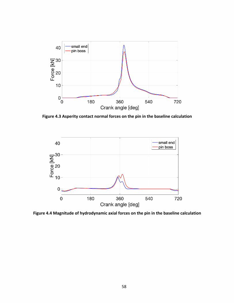
58
Figure 4.3 Asperity contact normal forces on the pin in the baseline calculation
Figure 4.4 Magnitude of hydrodynamic axial forces on the pin in the baseline calculation

59
Figure 4.5 Magnitude of asperity contact axial forces on the pin in the baseline calculation
Figures 4.4-4.5 show the magnitude of the axial forces on the pin. An axial force is the
integration of pressure after projecting to the axial direction of the piston (𝑧). The forces are
similar with the normal forces, indicating that the pressures are concentrated on the top and
bottom of the interfaces. Note that the axial forces from the small end and the pin boss are in
opposite directions.
The net axial force on the pin, which is shown in Figure 4.6, provides its acceleration and
is consistent with Figure 4.1.
Figure 4.6 Net axial force on the pin in the baseline calculation

60
4.1.3 Rotation of the pin
In general, the friction force between the pin and the small end drives the pin to rotate
with the con rod, whereas the friction force from the pin boss keeps the pin from rotating. On
the other hand, the coefficient of friction for boundary lubrication is the same on the two
interfaces in the baseline calculation and is much higher than the coefficient in the
hydrodynamic lubrication regime.
As a result, the pin has the tendency to follow whoever has the higher asperity contact
normal force with it. Figure 4.7 shows the net asperity contact normal force on the pin. It is
defined as the contact normal force from the small end bearing subtracting the force from the
pin boss. Figure 4.8 shows the angular velocities of the con rod and the pin.
Figure 4.7 Net asperity contact normal force on the pin in the baseline calculation

61
Figure 4.8 Angular velocities of con rod and pin in the baseline calculation
There is a connection between the patterns of the rotation and the axial acceleration of
the pin. When the acceleration of the pin is positive in Figure 4.1, there is more contact force
from the small end, which is pushing it upwards, and vice versa. Thus, when the piston is closer
to the TDC (around 0/720 CA and 360 CA), the pin stays with the pin bore and does not rotate.
When the piston is closer to the BDC (around 180 and 540 CA), the pin rotates with the con rod.
There is an exception between 360 and 450 CA, when the pin is accelerating downwards
but rotating with the con rod. This is the most critical period of time during the entire engine
cycle, as the combustion pressure above the piston is so high that both of the interfaces are
generating tremendous amount of pressures. The reason of this exception will be analyzed in
section 4.2.
4.1.4 Friction force and power loss
Figures 4.9 shows the friction forces from the small end and the pin boss, which can
reach 4000 Newtons. Figure 4.10 shows the net friction force on the pin, which determines its
rotation in Figure 4.8. The magnitude of the net friction force is much smaller than the
magnitude on individual interface, indicating a very stiff system.

62
Figure 4.11 shows the effective coefficient of friction in the boundary lubrication regime
at each interface. As analyzed before, the interface without relative rotation has a coefficient
less than the nominal value.
Figure 4.9 Friction forces on the pin in the baseline calculation
Figure 4.10 Net friction force on the pin in the baseline calculation

63
Figure 4.11 Effective coefficient of friction in boundary lubrication in the baseline calculation
As shown in Figure 4.8, the maximum angular velocity of the con rod is around 100 rad
per second, which gives a velocity of 1m/s as the radius of the pin is roughly 0.01m. Although
the speed is low, the maximum friction force on the pin occurs at the same time as the
maximum velocity of the con rod at the beginning of the expansion stroke. As a result, the
friction generates high power loss. Figure 4.12 shows the friction power loss of the pin system,
which can attain several thousand Watts.
By contrast, the sliding speed of the piston is low when the friction between the piston
and the cylinder liner is high. Figure 4.13 shows a typical pattern of the sliding velocity of the
piston and the friction force with the liner. It is calculated with the piston skirt lubrication
model [9] using the data from a different engine for qualitative comparison.

64
Figure 4.12 Friction power loss in the baseline calculation
Figure 4.13 Typical traces of the piston sliding velocity and the friction force between the
piston and the cylinder from the piston skirt lubrication model
4.2 Oil Transport Pattern
In this section, the overall pattern of the distribution and transport of lubricating oil will
be investigated.
Figures 4.14-4.16 show the distribution of asperity contact pressure, hydrodynamic
pressure, and void ratio at 384 CA, where the peak cylinder pressure (PCP) attained in the
combustion chamber takes place. The expanded view of the pin surface is the same as Figure

65
1.4, where 𝑦 is the axial direction of the pin and 𝜑 is the circumferential direction with 0/360
degrees being the top of the original surface and 180 degree as the bottom. The areas circled
by the red lines are the interfaces with the small end and the pin boss.
In order to balance the combustion pressure on the piston, the pin is in contact with the
piston pin boss at the top of their interface. The consequent force is in turn balanced by the
force from small end bearing at the bottom of the other interface. These areas will be referred
to as critical regions.
In the following subsections, some adjustments will be made to the plots of
distributions for simplicity and illustration
• Only half of the interfaces will be shown because of symmetry.
• The interface between the pin and the pin boss will be shifted by 180 degree in
the circumferential direction so that the critical regions on the interfaces are
aligned.
Figure 4.14 Distribution of asperity contact pressure at 384 CA in the baseline calculation

66
Figure 4.15 Distribution of hydrodynamic pressure at 384 CA in the baseline calculation
Figure 4.16 Distribution of void ratio at 384 CA in the baseline calculation

67
4.2.1 Intake stroke
Figure 4.17 shows the distribution of pressures at 90 CA, when neither the pin nor the
con rod is rotating. The red arrows represent the oil flow rate into/out of the boundaries of the
interfaces in the pin axial (𝑦) direction, and the black arrows show the oil flow rate in the
circumferential (𝜑) direction. The left and right boundaries of the two interfaces are not aligned
because of the angle of the con rod.
Since there is no relative rotation, the circumferential oil flow is driven by pressure. On
one hand, oil is squeezed out of the interface in the areas where hydrodynamic pressure builds
up. On the other hand, in the partial film regions, oil is drawn into the interfaces.
After 90 CA, the piston and the pin start to decelerate, and the pin rotates against the
pin boss. As shown in Figure 4.18, oil will be brought from the right portion of the interface to
the center portion, which is the critical region. The large curved arrows in yellow illustrate the
overall path of oil transport.

68
Figure 4.17 Distribution of pressures and oil exchange at the boundaries at 90 CA in the
baseline calculation

69
Figure 4.18 Distribution of pressures and oil exchange at the boundaries at 135 CA in the
baseline calculation
4.2.2 Compression stroke
In the late compression stroke, the acceleration of the piston becomes negative, and the
pin stops rotating. As shown in Figure 4.19, the relative rotation between the pin and the small
end has the similar effect on the oil transport. Lubricant will be brought to the critical region of
the interface to build hydrodynamic pressure.

70
Figure 4.19 Distribution of pressures and oil exchange at the boundaries at 315 CA in the
baseline calculation
4.2.3 Expansion stroke
Figure 4.20 shows the pressure distributions and oil flow rate at the boundaries in the
early expansion stroke. Because of the large hydrodynamic pressure, oil will be pushed from
the critical regions back to the right portion of the interfaces.
Although the small end has lower total normal force than the pin bore, it has higher
asperity contact force and drags the pin to rotate. This is mainly because the interfaces
between the pin and the pin boss have around twice as much boundaries as the pin-small end
interface. Because of the assumption that ambient pressure is higher than the constant

71
cavitation pressure, more oil will be sucked into the pin-pin boss interfaces. Figure 4.21 shows
the cumulative amount of oil transport absorbed from ambient into the interfaces through the
boundaries. It is scaled without dimension.
Figure 4.20 Distribution of pressures and oil exchange at the boundaries at 380 CA in the
baseline calculation
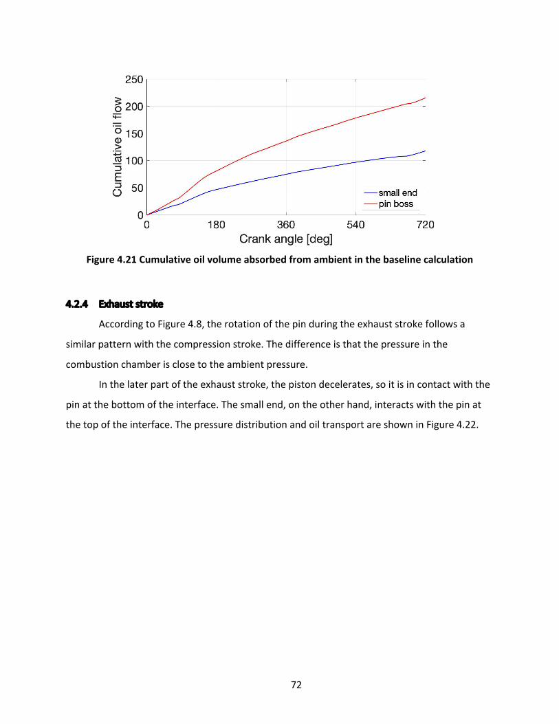
72
Figure 4.21 Cumulative oil volume absorbed from ambient in the baseline calculation
4.2.4 Exhaust stroke
According to Figure 4.8, the rotation of the pin during the exhaust stroke follows a
similar pattern with the compression stroke. The difference is that the pressure in the
combustion chamber is close to the ambient pressure.
In the later part of the exhaust stroke, the piston decelerates, so it is in contact with the
pin at the bottom of the interface. The small end, on the other hand, interacts with the pin at
the top of the interface. The pressure distribution and oil transport are shown in Figure 4.22.

73
Figure 4.22 Distribution of pressures and oil exchange at the boundaries at 675 CA in the
baseline calculation
4.2.5 Summary
The oil transport pattern on the interfaces is significantly affected by the axial
acceleration of the piston and the pin. In general, the pin will rotate with the con rod small end
when it has positive acceleration and stay with the piston pin boss when it has negative
acceleration.

74
Relative rotation is beneficial for the lubrication condition of the interfaces as it brings
oil to the critical regions. Therefore, it helps that the pin has relative rotation with both of its
mating components during an engine cycle.
Because the interface between the pin and the piston pin boss is divided into two
separate sections, it benefits from larger perimeter of boundary across which oil is absorbed
from ambient.
Although the results discussed in this section is based on an ideal setup where no
structural deformation is considered and some important parameters (roughness, sliding
coefficient of friction, installation clearance, etc.) are the same for both interfaces, it is helpful
to establish a basic oil transport pattern. It provides a powerful perspective that facilitates
further investigation in the effects of individual parameters.
4.3 Parametric Study
A parametric study is conducted to examine the effects of some critical parameters. This
study is to demonstrate the consistency of the model rather than identifying the trend in real
cases as the geometry is over-simplified.
4.3.1 Installation clearance
In the baseline calculation, both the installation clearances of the interfaces are 10
micrometers in radius. In this section, the effects of increasing each clearance are studied and
compared.
4.3.1.1 Between the pin and the pin boss
Figure 4.23 shows the normal forces in the calculation with different clearances
between the pin and the pin boss. The other clearance is 10 micrometers in all cases.
Between 90 CA and 360 CA, the cases with larger clearances have higher hydrodynamic
forces between the pin and the pin boss. This is mainly due to the amount of lubricant on the
interface. Figure 4.24 shows the average oil film thickness between the pin and the pin boss.
When the clearance is larger, the interface is able to gain more lubricant from the ambient. For

75
example, the curve for the 20-micrometer clearance not only grows faster than the other
curves, but also maintains more oil throughout the entire engine cycle.
After 360 CA, the load is so high that the minimum clearance between the pin and the
pin boss becomes very small for all the cases. As a result, the ability of the profiles to generate
hydrodynamic pressure is important. Figure 4.25 shows some artificial one-dimensional profiles
representing a cross-section of the pin-pin boss interface with different clearances. The black
curves represent the surfaces and the blue curves indicate the sliding velocity. The
hydrodynamic pressure was solved with the same minimum clearance, sliding velocity, and
boundary oil film thickness. It shows that a smaller clearance is able to generate higher
hydrodynamic force, which is the reason why there is more asperity contact force on the pin
boss at early expansion stroke when the clearance is larger.
Figure 4.23 Normal forces on the pin with different pin-pin boss installation clearances

76
Figure 4.24 Average oil film thickness between pin and pin boss with different pin-pin boss
installation clearances
Figure 4.25 Hydrodynamic pressure on a cross-section with the same boundary conditions
and different installation clearance.
Figure 4.26 shows the angular velocities of the pin. The most significant difference
occurs in the late compression stroke, when the pin in the 20-micrometer case rotates with the
small end. This is because it has higher hydrodynamic force and therefore lower asperity
contact between the pin and the pin boss.

77
Figure 4.26 Angular velocities of the pin with different pin-pin boss installation clearances
4.3.1.2 Between the pin and the small end bearing
Figure 4.27 shows the normal forces in the calculation with different clearances
between the pin and the small end. The other clearance is 10 micrometers in all cases.
Both interfaces will have more contact when the clearance gets larger. The changes on
the small end are because of the same reason discussed above, whereas the higher asperity
contact pressure on the pin boss can be attributed to the rotation of the pin.
During the late intake stroke and the early compression stroke (90-270 CA), the load is
not high, and the minimum oil film thickness is not as low as PCP timing. Compared to the
baseline calculation, the relative sliding between pin and small end helps build hydrodynamic
pressure. Therefore, although the small end has larger total force than the pin boss, the
contribution from asperity contact is actually less, and the pin stays with pin boss, as shown in
Figure 4.28. As a result, less amount of oil will be brought to the critical region to be used later.

78
Figure 4.27 Normal forces on the pin with different pin-small end installation clearances
Figure 4.28 Angular velocities of the pin with different pin-small end installation clearances

79
4.3.2 Roughness of the surfaces
According to the asperity contact sub-model introduced in Chapter 2, with the same
minimum clearance on an interface, the asperity contact pressure will be much lower when the
roughness is smaller. This means that in the case with lower roughness, the two surfaces can be
closer to each other to generate higher hydrodynamic pressure without producing excessive
contact in the meantime.
In the baseline calculation, both the pin boss and the small end bearing have a surface
roughness of 0.8 micrometer. In this section, the effects of decreasing each roughness are
studied and compared.
Figure 4.29 shows the normal forces in the calculation with different roughness on both
the pin boss and the small end bearing. It is obvious that smaller roughness leads to lower
asperity contact pressure and higher hydrodynamic pressure.

80
Figure 4.29 Normal forces on the pin with different roughness on the pin boss and the small
end bearing
4.3.2.1 Roughness of the pin boss
Figure 4.30 shows the normal forces in the calculation with different roughness only on
the pin boss. The roughness on the small end bearing is 0.8 micrometer in all cases.
The asperity contact force between the pin and the pin boss decreases with the
roughness. However, the contact on the other interface becomes larger.
This is a direct illustration of the subtle connection between the two interfaces. When
the pin-pin boss interface has lower asperity contact, it will have less friction and therefore
more relative rotation. Consequently, the pin-small end interface will have less relative
rotation, which results in less lubricant brought to the critical region and more asperity contact.

81
However, because of the limited relative rotation, the friction force between the pin and
the small end bearing is decreased as well, as shown in Figures 4.32. Figure 4.33 shows the
friction force between the pin and the pin boss, and Figure 4.34 shows the total friction power
loss and friction mean effective pressure (FMEP) of the system.
Figure 4.30 Normal forces on the pin with different pin boss roughness

82
Figure 4.31 Angular velocities of the pin with different pin boss roughness
Figure 4.32 Friction force between the pin and the small end bearing with different pin boss roughness

83
Figure 4.33 Friction force between the pin and the pin boss with different pin boss roughness
Figure 4.34 Friction power loss and FMEP with different pin boss roughness
4.3.2.2 Roughness of the small end bearing
Figures 4.35 and 4.36 show the angular velocities and normal forces in the calculation
with different roughness only on the small end bearing. The roughness on the pin boss is 0.8
micrometer in all cases.

84
The situation is similar to the previous subsection. The surface with lower roughness has
less asperity contact while the other surface has more. The pin is rotating less closely with the
con rod.
Figure 4.35 Angular velocities of the pin with different small end bearing roughness
Figure 4.36 Normal forces on the pin with different small end bearing roughness

85
4.3.3 Coefficient of friction
The role of the coefficient of friction in the boundary lubrication regime is
straightforward. With the similar magnitudes of asperity contact force, the interface with a
higher friction coefficient will have higher potential in generating friction force and prevent
relative rotation.
4.3.3.1 Coefficient of friction between pin and pin boss
Figures 4.37 and 4.3 show the rotation of the pin and the normal forces with different
coefficients of friction between the pin and the pin boss. The coefficient of the other interface
is 0.10.
When the friction coefficient between the pin and the pin boss is larger, it will be
difficult for the pin to rotate with the con rod. This is because once the pin starts to rotate
against the pin boss, a much higher friction force will arise and stop the rotation. Therefore, the
lubrication condition on the interface is deteriorated because less oil can be redistributed to
the critical region. As a result, there will be higher asperity contact between the pin and the pin
boss.
Figure 4.37 Angular velocities of the pin with different coefficient of friction between pin and pin bore

86
Figure 4.38 Normal forces on the pin with different coefficient of friction between pin and pin
bore
Figure 4.39 Sliding oil flow rate into the critical region of the small end with different coefficient of friction between pin and pin bore

87
On the other hand, although the pin-small end interface has relative relation during the
entire engine cycle, it has more contact as well. This is exactly due to the non-stopping sliding
between the surfaces.
Figure 4.39 shows the net oil flow rate into the critical region of the small end bearing
due to sliding motion. Here the ‘critical region’ is defined as the area centered around the very
bottom of the small end bearing with a circumferential range of 0.6 rad, as shown by the green
box in Figure 4.40. The flow rate pattern with modified coefficient of friction is significantly
different from the baseline case.
As shown in Figure 4.37, in the baseline case, the angular velocity of the con rod is
almost always smaller than or equal to the pin (the blue curve is always above or overlap with
the black dotted curve). This means that the pin can rotate against the small end only in one
direction, which is from right to the left in Figure 4.41. On the other hand, the clearance around
the critical region is usually the lowest in the entire circumference. This leads to the
accumulation of lubricant to the right of the critical region as discussed in section 4.2.
In the other cases, the pin can rotate against the small end in both directions. Thus, the
oil will not be accumulated as a long-term effect. The only exception is the extruded part of the
interface, as shown in the red circle in Figure 4.40, which receives Couette flow from outside
the boundaries. Therefore, while the baseline case can build hydrodynamic pressure along the
entire pin axis, the other cases only have hydrodynamic pressure in limited area.

88
Figure 4.40 Pressure distributions and oil flow through the boundaries at 135 CA with
different coefficient of friction between pin and pin bore
Figure 4.41 Pressure distributions and oil flow through the boundaries at 315 CA with
different coefficient of friction between pin and pin bore

89
4.3.3.2 Coefficient of friction between pin and small end bearing
Figure 4.42 shows the normal forces on the pin with different coefficients of friction
between the pin and the small end bearing. The coefficient of the other interface is 0.10.
The effects are similar to the previous subsection. Both interfaces will have higher
asperity contact if the friction coefficient is larger.
As shown in Figure 4.43, with larger friction coefficient between the pin and the small
end bearing, the pin will follow the rotation of the con rod during most of the engine cycle.
Figure 4.42 Normal forces on the pin with different coefficient of friction between pin and
small end bearing

90
Figure 4.43 Angular velocities of the pin with different coefficient of friction between pin and small end bearing
Figures 4.44 and 4.45 show the friction force and effective friction coefficient between
the pin and the small end bearing. In the baseline calculation, the pin stays with the pin boss in
the late compression stroke (270-360 CA) and its effective friction coefficient with the small end
bearing reaches the upper bound. As the higher upper bound is increased from 0.10 to 0.15,
more friction force can be generated so that the pin instead rotates with the small end.
However, when the upper bound further increases to 0.20, the extra potential for friction
forces will not be utilized. Therefore, both the friction force and the effective coefficient do not
change anymore. This is also the situation in the early expansion stroke (360-450 CA).
As a result, as long as the other interface stays the same, the overall friction loss will not
increase by much from 0.15 to 0.20, as shown in Figure 4.46.

91
Figure 4.44 Friction force between the pin and the small end bearing with different coefficient
of friction
Figure 4.45 Effective coefficient of friction between the pin and the small end bearing with
different sliding coefficient of friction
Figure 4.46 Friction power loss and FMEP with different coefficient of friction between pin
and small end bearing

92
4.3.4 Engine speed
Figure 4.47 shows the normal forces on the pin in the cases with different engine
speeds. When the speed is lower, there is less hydrodynamic pressure builds up in the early
expansion stroke. This is because less amount of oil is brought to the critical region by the
sliding motion, as shown in Figure 4.48.
Figure 4.47 Normal forces on the pin with different engine speeds
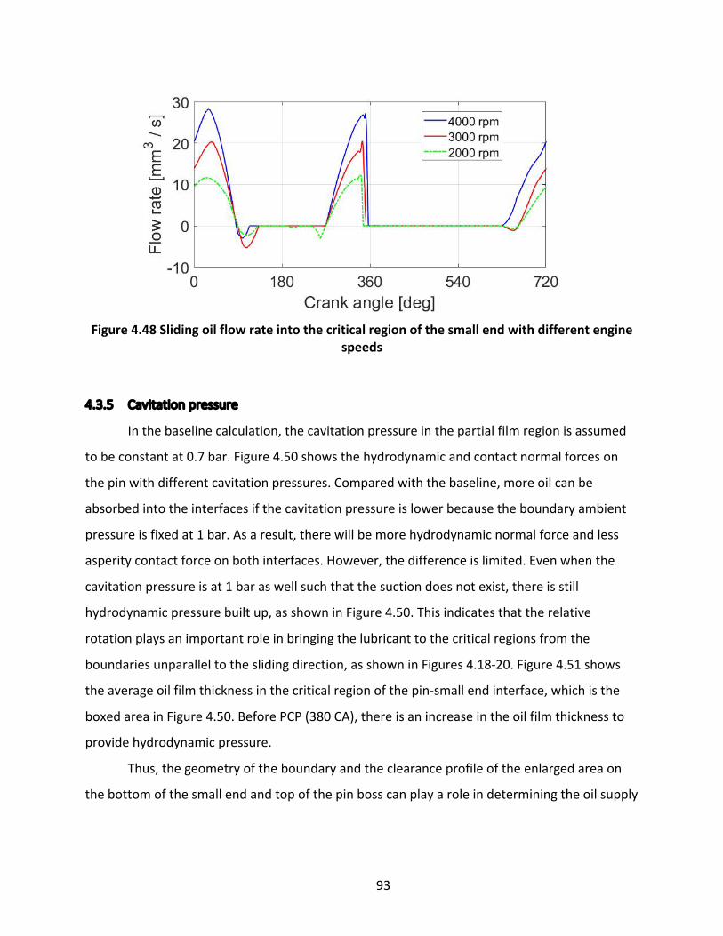
93
Figure 4.48 Sliding oil flow rate into the critical region of the small end with different engine
speeds
4.3.5 Cavitation pressure
In the baseline calculation, the cavitation pressure in the partial film region is assumed
to be constant at 0.7 bar. Figure 4.50 shows the hydrodynamic and contact normal forces on
the pin with different cavitation pressures. Compared with the baseline, more oil can be
absorbed into the interfaces if the cavitation pressure is lower because the boundary ambient
pressure is fixed at 1 bar. As a result, there will be more hydrodynamic normal force and less
asperity contact force on both interfaces. However, the difference is limited. Even when the
cavitation pressure is at 1 bar as well such that the suction does not exist, there is still
hydrodynamic pressure built up, as shown in Figure 4.50. This indicates that the relative
rotation plays an important role in bringing the lubricant to the critical regions from the
boundaries unparallel to the sliding direction, as shown in Figures 4.18-20. Figure 4.51 shows
the average oil film thickness in the critical region of the pin-small end interface, which is the
boxed area in Figure 4.50. Before PCP (380 CA), there is an increase in the oil film thickness to
provide hydrodynamic pressure.
Thus, the geometry of the boundary and the clearance profile of the enlarged area on
the bottom of the small end and top of the pin boss can play a role in determining the oil supply

94
to and pressure generation of the contact area. This model can be used to help optimize related
design features.
Figure 4.49 Normal forces on the pin with different cavitation pressures

95
Figure 4.50 Hydrodynamic pressure [bar] at 380 CA with different cavitation pressures
Figure 4.51 Average oil film thickness in the critical region of the pin-small end interface
4.4 Effects of Deformation of the Pin
As stated in Chapter 2, only the component of deformations in the radial direction of
the pin will be included, and all of them are assumed to be elastic.
Figure 4.51 shows the magnified radial deformation on the pin with a simple loaded
condition. Each end of pin takes a normal force of 1000 Newtons on the top, while another
normal force of 2000 Newtons is applied to the middle of the pin on the bottom.
The total deformation can be roughly decomposed into the following parts.
• Bending

96
• Ovality of the cross-section
• Local distortion near the loaded places
In Figure 4.51, the contribution of bending at the two ends is around 1 micrometer.
Since the actual loads on the pin can attain an order of magnitude of 10 thousand Newtons, the
effect of bending will be significant.
Figures 4.52 and 4.53 show the normal forces on the interfaces and the angular
velocities of the pin. The ‘no deform.’ label represents the baseline calculation discussed in the
previous chapter, while ‘deform.’ stands for the case with the deformation of the pin included.
Figure 4.52 Deformation of the pin with two 1000N forces at the ends and a 2000N force in
the middle

97
Figure 4.53 Normal forces on the interfaces with rigid and elastic pins
Figure 4.54 Angular velocities of rigid and elastic pins

98
Compared with the baseline, the most pronounced difference of the case with an elastic
pin is that there is much less pin rotation during the engine cycle. The direct reason is the
higher asperity contact force between the pin and the pin boss, as shown in the bottom right of
Figure 4.52.
Figures 4.54 shows the distributions of hydrodynamic pressure, asperity contact
pressure, clearance, and deformation of the cases at 120 CA. The oil flow rate is illustrated by
the red arrows. During the late intake stroke, because the pin bends away from the outer edge
of the pin boss on the top of the interface, the large clearance makes it difficult to generate
either hydrodynamic pressure or contact pressure. In order to compensate it, the inner edge
has to be much closer to the pin. As a result, the contact on the pin boss is higher than the small
end bearing, and the pin will stay with the pin boss and rotate against the small end. Thus, the
asperity contact force between the pin and the small end bearing is smaller than that in the
baseline case.
In the late compression stroke, the load rises significantly due to the pressure in the
combustion chamber. As shown in Figure 4.55, the pressures are concentrated not only on the
inner edge of the pin boss, but also on the outer edge of the small end bearing. The edges,
therefore, have limited clearances between the surfaces. On the other hand, the pin is rotating
relatively with the small end and transporting oil to the critical region. The arrows in Figure 4.55
show that in the baseline case, some of the oil transport will be squeezed out of the interface
when it meets the existing hydrodynamic pressure that has been developed in almost the
entire critical region. However, when the pin is able to deform, the center of the critical region
will have higher clearance because of bending. Therefore, lubricant can be accumulated and
available in the following strokes.
As shown in Figure 4.56, at 500 CA, the accumulated oil will provide hydrodynamic
pressure in the center of the small end bearing, whereas in the baseline case the load is entirely
supported by asperity contact.

99
Figure 4.57 shows the friction power loss of the two cases. With deformation, there is
more power loss around the TDC of expansion stroke (360 CA) and less power loss in the later
expansion stroke. The overall loss is slightly higher than the baseline case.
Figure 4.55 Clearance, deformation, oil flow rate, and pressures on the interfaces at 120 CA

100
Figure 4.56 Clearance, deformation, oil flow rate, and pressures on the interfaces at 300 CA

101
Figure 4.57 Clearance, deformation, oil flow rate, and pressures on the interfaces at 500 CA

102
Figure 4.58 Friction power loss with rigid and elastic pins
4.5 Summary
In this chapter, the model was applied to a real gasoline engine to understand the
relation between the pin rotation and the lubrication of the two interfaces. For this purpose,
the profiles of small end and pin bore bearings and their thermal and mechanical deformations
are not considered to ease the analysis. The basic pattern in the interaction of the pin with the
small end and the pin boss was identified, and the effects of various design and operation
parameters were analyzed. The model was found to generate consistent results for the
mechanisms considered.
When the two interfaces are in the same condition in terms of installation clearance,
surface roughness, coefficient of friction, and oil supply at the boundaries, the system will
follow a certain kind of symmetry, which originally comes from the axial acceleration pattern of
the pin. During approximately one half of the engine cycle, there is higher load between the pin
and the small end bearing, and the pin rotates with the small end, bringing oil to the top of the
pin-pin boss interface. During the other half of the cycle, the pin stays with the pin boss and
brings oil to the bottom of the pin-small end interface. Since the amounts of cumulative
rotation of the pin against both pin boss and small end are similar, both interfaces are to some
extent equally lubricated.

103
On the other hand, the system is very stiff in the sense that the forces on the pin from
each interface are more than two orders of magnitude larger than the corresponding net
forces. Therefore, a slight change in the condition of one interface will alter the behavior on the
other as well.
On each interface, the product of the normal asperity contact force and the sliding
coefficient of friction determines an upper bound of the friction force or friction potential,
while the lower bound is zero. As the angular inertia of the pin is much less than the friction
moment of either interface, the friction torque from two interfaces are approximately
balanced. If the pin stays with one interface, it means that this interface has higher friction
potential than the other interface. For instance, if the interface of pin and small end is
frictionless, the friction between the pin and pin boss will be zero no matter how large its
friction potential is. This concept of friction potential and effective friction coefficient is helpful
in understanding the rotation of the pin and its relationship with the lubrication of two
interfaces. Therefore, in order to reduce friction loss, only one of the interfaces need to be
improved. This has been shown by the parametric study where the friction power is smaller
when one of the interfaces has lower roughness or sliding coefficient of friction. The model’s
ability to reflect this interesting process shows the adequacy of the approximation of stick-slip
friction used in this work.
The opposite is also true. If the asperity contact or friction force on one interface is
increased, the other interface will be negatively affected as well, and the overall friction loss of
the system will be higher. An example will be shown in the next Chapter, where the
deformation of the pin leads to concentrated contact pressure on the edge of the pin boss.

104
Chapter 5 Application to a Modern Gasoline Engine
5.1 Input Setup
In this section, the model is applied to a gasoline engine. The important parameters are
shown in Table 5.1.
The profile of the pin boss is included in the form of the variance from the nominal
radius in the radial direction. It consists of the initial cold shape and the expansion due to
thermal load, which are shown respectively in Figures 5.1 and 5.2. Figure 5.3 shows total
variance. The pin boss features axial oil slots, which are treated in the same way as the
boundary regions, as shown in Figure 2.2.
Table 5.1 Specification and running condition of the gasoline engine studied in section 5.1
Stroke 92.8 mm
Cylinder bore diameter 82.5 mm
Con rod length 144 mm
Engine speed 2000 rpm
Peak cylinder pressure 15.6 bar
Installation clearance between pin and small end bearing 20 µm
Installation clearance between pin and piston pin boss 20 µm
Pin diameter 21 mm
Roughness of pin 0.1 µm
Roughness of small end bearing 0.8 µm
Roughness of piston pin boss 0.8 µm
Boundary friction coefficient between pin and small end bearing 0.10
Boundary friction coefficient between pin and piston pin boss 0.10
Cavitation pressure 0.7 bar
Initial oil film thickness on the interfaces 5 µm

105
Figure 5.1 Cold radial variance (micrometer) of the pin
Figure 5.2 Additional radial variance (micrometer) of the pin boss due to thermal load

106
Figure 5.3 Total radial variance (micrometer) of the pin
The total radial variances for the pin and the con rod small end bearing are assumed to
be uniform at 20 micrometers.
The structural deformations of both the pin and the pin boss are included in the
calculation, while the small end bearing is assumed to be rigid.
The pressure in the combustion chamber is shown in Figure 5.4.
Figure 5.4 Combustion pressure trace used in the calculation

107
5.2 Results with Rigid and Elastic Components
Figures 5.5 shows the normal forces on the pin from the calculation of the following
cases
• No deformation is considered. All the components are rigid.
• Elastic deformation of the pin is considered.
• Elastic deformation of both the pin and the pin boss is considered.
Figures 5.6 and 5.7 show the friction forces, friction power loss, and FMEP for these
cases. When only the pin is deforming, there will be less asperity contact and friction between
the pin and the pin boss around expansion TDC. When the deformation of the pin boss is also
considered, the situation will be slightly further improved.
Figure 5.5 Normal forces on the pin with different considerations of deformation

108
Figure 5.6 Friction force between the pin and the pin boss with different considerations of
deformation
Figure 5.7 Friction power loss and FMEP between the pin and the small end with different
considerations of deformation
Figure 5.8 shows the rotation of the pin. The patterns are similar in the cases, especially
before the early expansion stroke. Therefore, the difference in the friction loss should be
mainly attributed to the direct effect of deformation on the clearance.
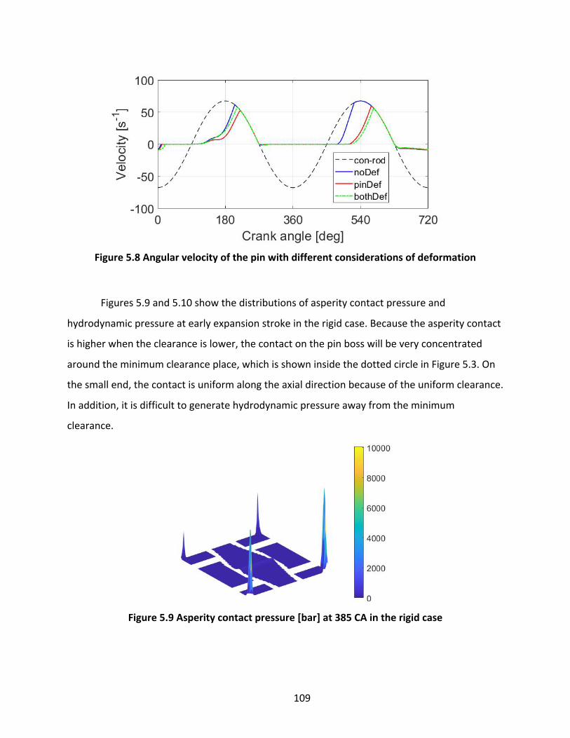
109
Figure 5.8 Angular velocity of the pin with different considerations of deformation
Figures 5.9 and 5.10 show the distributions of asperity contact pressure and
hydrodynamic pressure at early expansion stroke in the rigid case. Because the asperity contact
is higher when the clearance is lower, the contact on the pin boss will be very concentrated
around the minimum clearance place, which is shown inside the dotted circle in Figure 5.3. On
the small end, the contact is uniform along the axial direction because of the uniform clearance.
In addition, it is difficult to generate hydrodynamic pressure away from the minimum
clearance.
Figure 5.9 Asperity contact pressure [bar] at 385 CA in the rigid case

110
Figure 5.10 Hydrodynamic pressure [bar] at 385 CA in the rigid case
When the pin is elastic, the deformation at peak cylinder pressure is shown in Figure
5.11. It not only has local distortion in the areas with the highest pressures, but also bends
downwards. Because of the bending, the clearance at the edges of the pin-small end interface
is lower than the middle, as shown in Figure 5.12. Consequently, the pressures are higher near
the edges, as shown in Figures 5.13 and 5.14.
On the other hand, the deformation makes the pin and pin boss conform more to each
other, so the asperity contact at their interface is more spread, and more hydrodynamic
pressure can be generated compared to the rigid case.
Figure 5.11 Magnified deformation [𝝁m] of the pin at 385 CA in the case with elastic pin

111
Figure 5.12 Clearance between pin and small end at 385 CA
Figure 5.13 Asperity contact pressure [bar] at 385 CA in the case with elastic pin
Figure 5.14 Hydrodynamic pressure [bar] at 385 CA in the case with elastic pin

112
Figure 5.15 shows the deformation of the pin boss at 385 CA when it is elastic as well. In
this case, it will conform even better with the pin, and the lubrication condition will be further
improved. Figure 5.16 shows the hydrodynamic deformation.
Figure 5.15 Magnified deformation [𝝁m] of the pin boss at 385 CA in the case with elastic pin
and pin boss
Figure 5.16 Hydrodynamic pressure [bar] at 385 CA in the case with elastic pin and pin boss
The change in the asperity contact due to deformation is in the different direction from
what was discussed in the previous parametric study. This is because in the previous chapter,
all the surfaces are originally cylindrical and fit each other well. When deformation occurs,
there will be places with lower local clearance so that the contact becomes more concentrated.
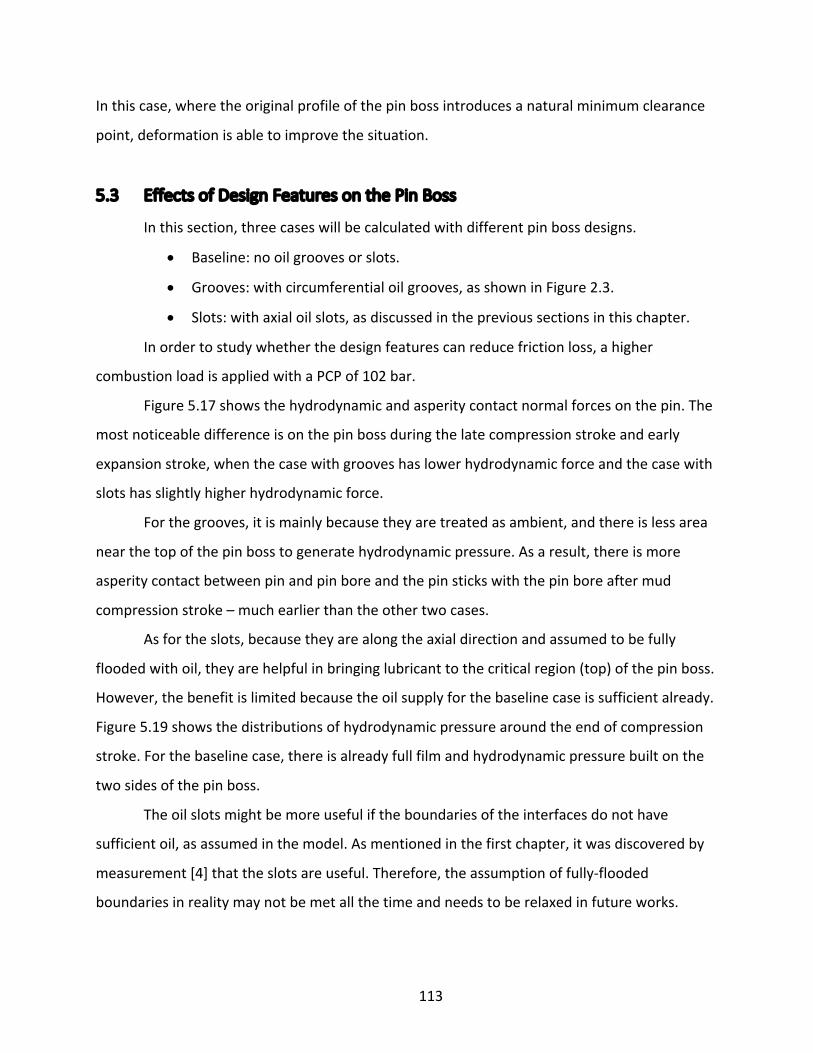
113
In this case, where the original profile of the pin boss introduces a natural minimum clearance
point, deformation is able to improve the situation.
5.3 Effects of Design Features on the Pin Boss
In this section, three cases will be calculated with different pin boss designs.
• Baseline: no oil grooves or slots.
• Grooves: with circumferential oil grooves, as shown in Figure 2.3.
• Slots: with axial oil slots, as discussed in the previous sections in this chapter.
In order to study whether the design features can reduce friction loss, a higher
combustion load is applied with a PCP of 102 bar.
Figure 5.17 shows the hydrodynamic and asperity contact normal forces on the pin. The
most noticeable difference is on the pin boss during the late compression stroke and early
expansion stroke, when the case with grooves has lower hydrodynamic force and the case with
slots has slightly higher hydrodynamic force.
For the grooves, it is mainly because they are treated as ambient, and there is less area
near the top of the pin boss to generate hydrodynamic pressure. As a result, there is more
asperity contact between pin and pin bore and the pin sticks with the pin bore after mud
compression stroke – much earlier than the other two cases.
As for the slots, because they are along the axial direction and assumed to be fully
flooded with oil, they are helpful in bringing lubricant to the critical region (top) of the pin boss.
However, the benefit is limited because the oil supply for the baseline case is sufficient already.
Figure 5.19 shows the distributions of hydrodynamic pressure around the end of compression
stroke. For the baseline case, there is already full film and hydrodynamic pressure built on the
two sides of the pin boss.
The oil slots might be more useful if the boundaries of the interfaces do not have
sufficient oil, as assumed in the model. As mentioned in the first chapter, it was discovered by
measurement [4] that the slots are useful. Therefore, the assumption of fully-flooded
boundaries in reality may not be met all the time and needs to be relaxed in future works.

114
Figure 5.20 shows the friction forces between the pin and the pin boss and the FMEP
associated with the pin. The effects on FMEP are not significant from both variants. The FMEP
increases from the baseline case by around 4% with grooves added, and decreases by 2.5% with
slots added.
Figure 5.17 Normal forces on the pin with different pin boss designs

115
Figure 5.18 Angular velocity of the pin with different pin boss designs
Figure 5.19 Hydrodynamic pressure distribution at 340 CA with different pin boss designs

116
Figure 5.20 Friction force between pin and pin boss and FMEP with different pin boss designs

117
Chapter 6 Conclusions
6.1 Conclusions
The main challenge of the pin lubrication is that its primary motion or pin rotation is
unknown. The pin rotation is determined by the competition of the forces generated in the
small end and piston bearing interfaces, where the pin rotation plays a central role in the
outcome of oil transport, pressure, and friction. Thus, understanding the lubrication of the
piston pin needs to resolve the coupling of the primary motion of the pin, oil transport on the
interfaces, and oil exchange with the surroundings. Additionally, both hydrodynamic and
boundary lubrication are highly dependent on the exact geometry of the mating parts during
operation. Therefore, coupling the thermal and mechanical deformation of the pin, pin bore,
and small end is essential for the model to reflect the reality. Furthermore, the problem is
numerically challenging as the magnitude of the two competing forces at the two interfaces is
much greater than the inertia of the pin rotation. The present work shows that a stable model
with consistent results can be realized by employing adequate lubrication sub-models with oil
conservation and a stable algorithm.
The present work has been limited to model development and examination of the
consistency of the model in reflecting the built-in physics and the effects of the design and
operating parameters. Comparing the model prediction and the real measurement requires
accurate data on temperature, thermal and structural deformation, and geometry change due
to wear, and is beyond the scope of this work.
Preliminary results do show that substantial friction power loss can come from this
system despite its relatively slow sliding speed. This is because high magnitude of contact force
and the alignment of the timing between highest friction force and highest sliding speed.
Furthermore, the friction is mainly contributed by the boundary lubrication while hydrodynamic
friction is almost negligible. As pin is free, the friction can thus be effectively reduced by
enhancing the hydrodynamic effect in only one interface, which includes ensuing oil supply to

118
the contact regions and favorable clearance shape during engine operation. The current model
has the capability to help make necessary design changes toward that direction.
The friction potential developed in this work is a useful concept to help understand the
rotation of the pin. When the coefficient of friction of the boundary lubrication of the two
interfaces are the same, it has been found that the reciprocating nature of the piston leads to a
pattern where the pin rotates with the connecting rod during half of the engine cycle, and stays
with the piston during the other half. Because of the larger width on the bottom of the small
end and the top of the pin boss, this pattern is favorable for bringing oil to the regions with the
highest load. More friction will be generated if the pin rotates more with either of the
components. This might be able to provide some guidance for new designs.
As the first step to establish a comprehensive engineering model to understand the pin
lubrication, this work not only lays a foundation but also helps gain a great deal of insights to
the complex interactions involved in the pin lubrication.
6.2 Future Work
A number of simplifications in the present model can be improved in the future. First of
all, more factors need to be added for more accurate simulation, such as the structural
deformation of the con rod small end, and the effects of temperature and shear stress on the
viscosity of the lubricant.
On the other hand, there are special design features for different engines in the market.
For instance, in some commercial vehicle diesel engines, there is an oil bore in the shank of the
connecting rod through which oil can be transported to lubricate the small end bearing; there
are also cases where the hole on the piston pin has an offset such that the inner and outer
surfaces of the pin are not concentric. The current model can be improved accordingly in order
to consider such design features.
The oil supply to the boundaries of the interfaces, if found not necessarily sufficient
temporally and spatially, will be a subject of further work as well. While relaxing the presently

119
fully-flooded boundary condition in the model is straightforward, where and when the
boundaries may become starved need more work assisted with experimental findings.
Finally, the results of the model, especially the friction on the pin, can be used to
improve the other models. As an example, the piston skirt lubrication model [9] neglects the
friction force between the pin and the pin boss when calculating the torque of the piston. This
assumption can be dropped with information provided by the pin lubrication model.

120
References
[1] Johnson, T., & Joshi, A. (2017). Review of Vehicle Efficiency and Emissions (No. 2017-01-0907). SAE Technical Paper.
[2] Holmberg, K., Andersson, P., & Erdemir, A. (2012). Global energy consumption due to friction in passenger cars. Tribology international, 47, 221-234.
[3] Richardson, D. E. (2000). Review of power cylinder friction for diesel engines. Transactions of the ASME, Journal of Engineering for Gas Turbines and Power, 122(4), 506-519.
[4] Meiser, J., Deuß, T., Ehnis, H., & Künzel, R. (2017). Friction Power Measurements of a Fired Gasoline Engine Influence of Piston Pin Bore. MTZ worldwide, 78(1), 58-62.
[5] Bai, D. (2012). Modeling piston skirt lubrication in internal combustion engines (Doctoral dissertation, Massachusetts Institute of Technology).
[6] Totaro, P. (2014). Modeling piston secondary motion and skirt lubrication with applications (Master’s thesis, Massachusetts Institute of Technology).
[7] Meng, Z. (2017). Numerical investigation of the piston skirt lubrication in heavy duty diesel engines (Master’s thesis, Massachusetts Institute of Technology).
[8] Meng, Z., Ahling, S., & Tian, T. (2019). Modeling of Oil Transport between Piston Skirt and Cylinder Liner in Internal Combustion Engines. SAE International Journal of Advances and Current Practices in Mobility, 1(2019-01-0590), 1158-1168.
[9] Meng, Z., Zhang, L., & Tian, T. (2019). Study of Break-In Process and its Effects on Piston Skirt Lubrication in Internal Combustion Engines. Lubricants, 7(11), 98.
[10] Heiserman, D. L. (n.d.). Auto and Light-Truck Systems. Retrieved July 2, 2020, from http://www.waybuilder.net/freeed/Courses/15%20Transportation/AutoTruck03/AutoTruckShow.asp?iNum= 010102.
[11] Suhara, T., Ato, S., Takiguchi, M., & Furuhama, S. (1997). Friction and lubrication characteristics of piston pin boss bearings of an automotive engine (No. 970840). SAE Technical Paper.
[12] Iwasaki, H., Higasa, Y., Takiguchi, M., Sue, S., & Shishido, K. (2007, January). Effects of Design for Piston Pin and Bearing on State of Bearing Lubrication. In Internal Combustion Engine Division Fall Technical Conference (Vol. 48116, pp. 631-636).
[13] Clark, K., Antonevich, J., Kemppainen, D., & Barna, G. (2009). Piston pin dynamics and temperature in a CI Engine. SAE International Journal of Engines, 2(1), 91-105.
[14] Abed, G., Zou, Q., Barber, G., Zhou, B., Wang, Y., Liu, Y., & Shi, F. (2013). Study of the motion of floating piston pin against pin bore. SAE International Journal of Engines, 6(2), 990-998.
[15] Miura, K., Kobayashi, K., Yamakawa, N., Saruwatari, M., & Mihara, Y. (2015). Measurement of Oil Film Pressure in Piston Pin-Boss by Thin-Film Pressure Sensor (No. 2015-01-2040). SAE Technical Paper.
[16] Ligier, J. L., & Ragot, P. (2005). Piston pin: wear and rotating motion (No. 2005-01-1651). SAE Technical Paper.

121
[17] Fridman, V., Piraner, I., & Clark, K. (2006, January). Modeling of mixed lubrication conditions in a heavy duty piston pin joint. In Internal Combustion Engine Division Spring Technical Conference (Vol. 42061, pp. 741-748).
[18] Wang, D., Mian, O., Merritt, D., & Zhu, G. (2008). Elasto-Hydrodynamic Lubrication Analysis and Wear Prediction of Con rod Small-End Bush and Piston Pin Interface (No. 2008-36-0068). SAE Technical Paper.
[19] Bertocchi, L., Giacopini, M., & Dini, D. (2012, October). Analysis of the Lubrication Regimes at the Small End and Big End of a Con rod of a High Performance Motorbike Engine. In International Joint Tribology Conference (Vol. 45080, pp. 229-231). American Society of Mechanical Engineers.
[20] Shi, F. (2011). An analysis of floating piston pin. SAE International Journal of Engines, 4(1), 2100-2105.
[21] Ba, L., He, Z. P., Liu, Y. H., & Zhang, G. C. (2015). Analysis of piston-pin lubrication considering the effects of structure deformation and cavitation. Journal of Zhejiang University-SCIENCE A, 16(6), 443-463.
[22] Hu, Y., Cheng, H. S., Arai, T., Kobayashi, Y., & Aoyama, S. (1994). Numerical simulation of piston ring in mixed lubrication—a nonaxisymmetrical analysis. Journal of Tribology, Transactions of the ASME, 116, 470-478.
[23] Greenwood, J. A., & Tripp, J. H. (1970). The contact of two nominally flat rough surfaces. Proceedings of the institution of mechanical engineers, 185(1), 625-633.
[24] Bhushan, B. (1998). Contact mechanics of rough surfaces in tribology: multiple asperity contact. Tribology letters, 4(1), 1-35.
[25] Biboulet, N., & Lubrecht, A. A. (2018). Efficient solver implementation for Reynolds equation with mass-conserving cavitation. Tribology International, 118, 295-300.
[26] Rabinowicz, E. (1958). The intrinsic variables affecting the stick-slip process. Proceedings of the Physical Society, 71(4), 668.
[27] Karnopp, D. (1985). Computer simulation of stick-slip friction in mechanical dynamic systems.