modelling credit risk - home | bank of england

Centre for Central Banking StudiesModelling credit risk

Somnath Chatterjee

CCBS Handbook No. 34

Modelling credit risk Somnath Chatterjee

[email protected]

Financial institutions have developed sophisticated techniques to quantify and manage credit risk across different product lines. From a regulator’s perspective a clear understanding of the techniques commonly used would enhance supervisory oversight of financial institutions. The initial interest in credit risk models originated from the need to quantify the amount of economic capital necessary to support a bank’s exposures. This Handbook discusses the Vasicek loan portfolio value model that is used by firms in their own stress testing and is the basis of the Basel II risk weight formula.

The role of a credit risk model is to take as input the conditions of the general economy and those of the specific firm in question, and generate as output a credit spread. In this regard there are two main classes of credit risk models – structural and reduced form models. Structural models are used to calculate the probability of default for a firm based on the value of its assets and liabilities. A firm defaults if the market value of its assets is less than the debt it has to pay. Reduced form models assume an exogenous, random cause of default. For reduced form or default-intensity models the fundamental modelling tool is a Poisson process. A default-intensity model is used to estimate the credit spread for contingent convertibles (CoCo bonds).

The final section focusses on counterparty credit risk in the over-the-counter (OTC) derivatives market. It describes the credit value adjustment that banks make to the value of transactions to reflect potential future losses they may incur due to their counterparty defaulting. I would like to thank Abbie McGillivray for designing the layout of this Handbook. [email protected] Centre for Central Banking Studies, Bank of England, Threadneedle Street, London, EC2R 8AH The views expressed in this Handbook are those of the author, and are not necessarily of the Bank of England. Series editor: Andrew Blake, email [email protected] This copy is also available via the internet site at www.bankofengland.co.uk/education/ccbs/handbooks_lectures.htm © Bank of England 2015 ISSN: 1756-7270 (Online)

boe490482

Text Box

Handbook No. 34 Modelling credit risk 3

Contents

Introduction 5

1 Economic capital allocation 6Probability density function of credit losses

Calculating joint loss distribution using the Vasicek model

The Vasicek model and portfolio invariance

6

8

12

2 Structural credit risk models 13Equity and debt as contingent claims

Asset value uncertainly

Estimating the probability of default

Applying the Merton model

14

15

17

19

3 Reduced form models 20

Default intensity

Contingent convertible capital instruments

Pricing CoCo bonds

21

22

23

4 Counterparty credit risk 24Credit value adjustments

Expected exposures with and without margins

25

26

References 28

Appendix 29


Modelling credit risk Introduction

Credit is money provided by a creditor to a borrower (also referred to as an obligor as he or she has an obligation).

Credit risk refers to the risk that a contracted payment will not be made. Markets are assumed to put a price on this

risk. This is then included in the market’s purchase price for the contracted payment. The part of the price that is

due to credit risk is the credit spread. The role of a typical credit risk model is to take as input the conditions of the

general economy and those of the specific firm in question, and generate as output a credit spread.

The motivation to develop credit risk models stemmed from the need to develop quantitative estimates of the

amount of economic capital needed to support a bank’s risk taking activities. Minimum capital requirements have

been coordinated internationally since the Basel Accord of 1998. Under Basel 1, a bank’s assets were allotted via a

simple rule of thumb to one of four broad risk categories, each with a ‘risk weighting’ that ranged from 0%-100%.

A portfolio of corporate loans, for instance, received a risk weight of 100%, while retail mortgages – perceived to be

safer – received a more favourable risk weighting of 50%. Minimum capital was then set in proportion to the

weighted sum of these assets.

minimum capital requirement = 8% x ∑

Over time, this approach was criticised for being insufficiently granular to capture the cross sectional distribution of

risk. All mortgage loans, for instance, received the same capital requirement without regard to the underlying risk

profile of the borrower (such as the loan to value or debt to income ratio). This led to concerns that the framework

incentivised ‘risk shifting’. To the extent that risk was not being properly priced, it was argued that banks had an

incentive to retain only the highest risk exposures on their balance sheets as these were also likely to offer the

highest expected return.

In response, Basel II had a much more granular approach to risk weighting. Under Basel II, the credit risk

management techniques under can be classified under:

Standardised approach: this involves a simple categorisation of obligors, without considering their actual

credit risks. It includes reliance on external credit ratings.

Internal ratings-based (IRB) approach: here banks are allowed to use their ‘internal models’ to calculate

the regulatory capital requirement for credit risk.

These frameworks are designed to arrive at the risk-weighted assets (RWA), the denominator of four key

capitalisation ratios (Total capital, Tier 1, Core Tier 1, Common Equity Tier 1). Under Basel II, banks following the IRB

approach may compute capital requirements based on a formula approximating the Vasicek model of portfolio

credit risk. The Vasicek framework is described in the following section.

boe490482

Text Box

6 Handbook No. 34 Modelling credit risk

Under Basel III the minimum capital requirement was not changed, but stricter rules were introduced to ensure

capital was of sufficient quality. There is now a 4.5% minimum CET1 requirement. It also increased levels of capital

by introducing usable capital buffers rather than capital minima. See BCBS (2010). Basel III cleaned up the

definition of capital, i.e., the numerator of the capital ratio. But it did not seek to materially alter the Basel II risk-

based framework for measuring risk-weighted assets, i.e., the denominator of the capital ratio; therefore, the

architecture of the risk weighted capital regime was left largely unchanged. Basel III seeks to improve the

standardised approach for credit risk in a number of ways. This includes strengthening the link between the

standardised approach the internal ratings-based (IRB) approach.

1. Economic capital allocation

When estimating the amount of economic capital needed to support their credit risk activities, banks employ an

analytical framework that relates the overall required economic capital for credit risk to their portfolio’s probability

density function (PDF) of credit losses, also known as loss distribution of a credit portfolio. Figure 1 shows this

relationship. Although the various modelling approaches would differ, all of them would consider estimating such a

PDF.

Figure 1 Loss distribution of a credit portfolio

Probability density function of credit losses

Mechanisms for allocating economic capital against credit risk typically assume that the shape of the PDF can be

approximated by distributions that could be parameterised by the mean and standard deviation of portfolio losses.

Figure 1 shows that credit risk has two components. First, the expected loss (EL) is the amount of credit loss the

bank would expect to experience on its credit portfolio over the chosen time horizon. This could be viewed as the

normal cost of doing business covered by provisioning and pricing policies. Second, banks express the risk of the

portfolio with a measure of unexpected loss (UL). Capital is held to offset UL and within the IRB methodology, the

regulatory capital charge depends only on UL. The standard deviation, which shows the average deviation of

expected losses, is a commonly used measure of unexpected loss. The area under the curve in Figure 1 is equal to

100%. The curve shows that small losses around or slightly below the EL occur more frequently than large losses.

boe490482

Text Box


The likelihood that losses will exceed the sum of EL and UL – that is, the likelihood that the bank will not be able to

meet its credit obligations by profits and capital – equals the shaded area on the RHS of the curve and depicted as

stress loss. 100% minus this likelihood is called the Value-at- Risk (VaR) at this confidence level. If capital is set

according to the gap between the EL and VaR, and if EL is covered by provisions or revenues, then the likelihood

that the bank will remain solvent over a one-year horizon is equal to the confidence level. Under Basel II, capital is

set to maintain a supervisory fixed confidence level. The confidence level is fixed at 99.9% i.e. an institution is

expected to suffer losses that exceed its capital once in a 1000 years. Lessons learned from the 2007-2009 global

financial crisis, would suggest that stress loss is the potential unexpected loss against which it is judged to be too

expensive to hold capital. Regulators have particular concerns about the tail of the loss distribution and about

where banks would set the boundary for unexpected loss and stress loss. For further discussion on loss distributions

under stress scenarios see Haldane et al (2007).

A bank has to take a decision on the time horizon over which it assesses credit risk. In the Basel context there is a

one-year time horizon across all asset classes. The expected loss of a portfolio is assumed to be equal to the

proportion of obligors that might default within a given time frame, multiplied by the outstanding exposure at

default, and once more by the loss given default, which represents the proportion of the exposure that will not be

recovered after default. Under the Basel II IRB framework the probability of default (PD) per rating grade is the

average percentage of obligors that will default over a one-year period. Exposure at default (EAD) gives an estimate

of the amount outstanding if the borrower defaults. Loss given default (LGD) represents the proportion of the

exposure (EAD) that will not be recovered after default. Assuming a uniform value of LGD for a given portfolio, EL

can be calculated as the sum of individual ELs in the portfolio (Equation 1.1)

Equation 1.1 ∑

Unlike EL, total UL is not an aggregate of individual ULs but rather depends on loss correlations between all loans in

the portfolio. The deviation of losses from the EL is usually measured by the standard deviation of the loss variable

(Equation 1.2). The UL, or the portfolio’s standard deviation of credit losses can be decomposed into the

contribution from each of the individual credit facilities:

Equation 1.2 ∑

where denotes the stand-alone standard deviation of credit losses for the ith facility, and denotes the

correlation between credit losses on the ith facility and those on the overall portfolio. The parameter captures the

ith facility’s correlation/diversification effects with other instruments in the bank’s credit portfolio. Other things

being equal, higher correlations among credit instruments – represented by higher – lead to a higher standard

deviation of credit losses for the portfolio as a whole.

Basel II has specified the asset correlation values for different asset classes (BCBS 2006). But the theoretical basis

for calculating UL under the Basel II IRB framework stems from the Vasicek (2002) loan portfolio value model. See

BCBS (2005) for further explanation of the Basel II IRB formulae. A problem with the IRB approach is that it implies

excessive reliance on banks’ own internal models in calculating capital requirements as the standardised approach

boe490482

Text Box


did not provide a credible alternative method for capturing risks in banks’ trading portfolios. However, banks’

internal models have been found to produce widely differing risk weights for common portfolios of banking assets.

Part of the difficulty in assessing banks’ RWA calculations is distinguishing between differences that arise from

portfolio risk and asset quality and those that arise from differences in models. To identify differences between

banks’ internal models, regulators have undertaken a number of exercises in which banks applied internal models to

estimate key risk parameters for a hypothetical portfolio assets. This ensured that differences in calculated risk

weights are down to differences in banks’ modelling approaches, rather than differences in the risk of portfolios

being assessed. The following section discusses the Vasicek (2002) methodology to calculate the joint loss

distribution for a portfolio of bank exposures.

Calculating joint loss distribution using the Vasicek model

The Vasicek (2002) model assumes that the asset value of a given obligor is given by the combined effect of a

systematic and an idiosyncratic factor. It assumes an equi-correlated, Gaussian default structure. That is, each

obligor i defaults if a certain random variable falls below a threshold, and these are all normal and equi-

correlated. The asset value of the i-th obligor at time t is therefore given by:

Equation 1.3 1

Where S and Z are respectively the systematic and the idiosyncratic component and it can be proved that is the

asset correlation between two different obligors. See Box 1 for further details on the Vasicek loan portfolio model.

Here , , , … , are mutually independent standard normal variables. The Vasicek model uses three inputs to

calculate the probability of default (PD) of an asset class. One input is the through-the-cycle PD (TTC_PD) specific

for that class. Further inputs are a portfolio common factor, such as an economic index over the interval (0,T) given

by S. The third input is the asset correlation. . Then the term is the company’s exposure to the systematic

factor and the term 1 represents the company’s idiosyncratic risk.

A simple threshold condition determines whether the obligor i defaults or not.

default iff

where will be shown to be a function of TTC_PD.

Box 1 The Vasicek loan portfolio value model

Vasicek applied to firms’ asset values what had become the standard geometric Brownian motion model. Expressed as a stochastic differential equation,

Where is the value of the th firm’s assets, and are the drift rate and volatility of that value, and is a Wiener process or Brownian motion, i.e. a random walk in continuous time in which the change over any finite time period is normally distributed with mean zero and variance equal to the length of the period, and changes in separate time periods are independent of each other. Solving this stochastic differential equation one obtains the value of the th firm’s assets at time T as:

boe490482

Text Box


The Vasicek model can be interpreted in the context of a trigger mechanism that is useful for modelling credit risk.

A simple threshold condition determines whether the obligor defaults or not.

Integrating over S in equation 1.3 we denote the unconditional probability of default by ∗ (this is the TTC_PD):

Pr ∗

The probability of default conditional on can be written as:

| 11

|

It follows that the probability of default conditional on S is equal to:

Equation 1.4 | N N∗

1

∗

1 ∗

(1) √

The th firm defaults if , so the probability of such an event is

(2) ∗

where is easily derived from equation (1) and N is the cumulative normal pdf. That is, default of a single obligor happens if the value of a normal random variable happens to fall below a certain .

Correlation between defaults is introduced by assuming correlation in the processes, and thus in the terminal values, . In particular, it is assumed that the in equation (1) are pair-wise correlated according to factor .

Being normal and equi-correlated, each random variable can then be represented as the sum of two other random variables: one common across firms, and the other idiosyncratic:

with ~ 0,1 , ~ 0,1 . Hence the probability of default of obligor can also be written as

(3) ∗

∗ in equation (2) is the through-the-cycle average loss. … in equation (3) is the loss subject to credit conditions S. The proportion of loans in the portfolio that suffer default is given by the following pdf:

(4)

boe490482

Text Box


The distribution function of the proportion of losses that suffer default is given by two parameters, default

probability, p and asset correlation, (rho). Figure 2 shows the portfolio loss distribution with default probability (p

= 0.02 or 2%) and asset correlation ( 0.1 or 10%). This is the unconditional probability of default.

Figure 2 Unconditional loss distribution

In the Vasicek framework, two processes drive the cyclical level of a portfolio loss rate: the stochastic common

factor S and asset correlations . What follows is an economic interpretation of both these processes beginning

with the common factor S.

Given a macroeconomic scenario, an S can be computed, which can then be used in the Vasicek framework to

calculate the loss rate conditional to that specific scenario. The common component S may be viewed as

representing aggregate macro-financial conditions which can be extracted from observable economic data.

Aggregate credit risk depends on the stochastic common factor S, because when we face good economic times the

expected loss rate tends to below the long-term average, while during bad times the expected loss rate is expected

to be above the long-term average. In this framework, S is unobservable. Despite their latent nature, many macro-

economic and financial variables regularly collected contain relevant information on the state of economic and

financial conditions. If we can extract from each of these observables the common part of information, which

represent the state of aggregate conditions, then we can use this measure as the factor S in the Vasicek framework

and compute the conditional loss rate. It is through the estimated S that a specific macro-economic scenario is

taken into account in the default rate calculation. Therefore, S may be viewed as the macro-to-micro default part

of the framework whereby macroeconomic and credit conditions are translated into applicable default rates. The

Kalman filter algorithm can be used to compute S. The main advantage of this technique is that it allows the state

variables to be unobserved magnitudes.

boe490482

Text Box


Figure 3 Expected loss conditional on the common state factor

Figure 3 shows the expected loss conditional on the common factor, S where the latter has been estimated using

the Kalman filter. It can be seen from Figure 3 that S shows strong persistence. Thus bad realisations of S tend to be

followed by bad realisations of S and vice versa. S is a standard normal variable with a mean of 0 and a standard

deviation of 1. In normal times one would not expect to observe large negative magnitudes for S. But under stress S

would dip more significantly into negative territory.

The Appendix at the end of this Handbook demonstrates how S can be estimated empirically using the Kalman

filter algorithm. A detailed explanation of the Kalman filter can be found in Harvey (1989) and Durbin and

Koopman (2012).

Asset correlations ρ (rho) are a way to measure the likelihood of the joint default of two obligors belonging to the

same portfolio and, therefore, they are important drivers of credit risk. The role of correlations in the Vasicek

framework needs to be clarified. A portfolio with high correlations produces greater default oscillations over the

cycle S, compared with a portfolio with lower correlations. Correlations do not affect the timing of the default;

higher correlations do not imply that defaults earlier or later than other portfolios. Thus, during good times a

portfolio with high correlations will produce fewer defaults than a portfolio with low correlations. While in bad

times the opposite is true, high correlations are creating more defaults.

Some benchmark values of ρ (rho) are available from the regulatory regimes. The Basel II IRB risk-weighted

formulae, which are based on the Vasicek model, prescribes, for corporate exposures, correlations between 12%

and 24%, where the actual number is computed as a probability of default weighted average.

boe490482

Text Box


Following the Vasicek framework, two borrowers are correlated because they are both linked to the common factor

S. Clearly this is a simplification of the true correlation structure. However, it allows the Vasicek framework to

provide a straightforward calculation of the default risk of a portfolio.

The Vasicek model and portfolio invariance

Banks estimate the input parameters for the Vasicek model via their internal models. In order to make IRB

applicable across jurisdictions, the BCBS determined that an approach with ‘risk weights’ would be used to

determine capital requirements. The risk weights would be valid if a given asset will take the same risk weight

regardless of the portfolio it is added to. This property is called portfolio invariance.

In theory, portfolio-invariant risk weights can be used to limit the probability that losses exceed total capital

provided two assumptions are met. First, portfolios must be ‘asymptotically fine-grained,’ which means that each

loan must be of negligible size. Second, one must make an ‘asymptotic single risk factor’ (ASRF) assumption. The

ASRF assumption means that, while every loan is exposed to idiosyncratic risk, there is only one source of common

shocks. See Gordy (2003). One can think of the ASRF as representing aggregate macro-financial conditions, S, as

described above. Each loan may have different correlation with the ASRF, but correlations between loans are driven

by their link to that single factor, S. Violation of either of these assumptions would result in an incorrect

assessment of portfolio credit risk.

The ‘asymptotically fine-grained’ assumption treats the portfolio as being made up of an infinite number of

negligible exposures. In practice, however, real portfolios are usually lumpy. Lumpiness effectively decreases the

diversification of the portfolio, thereby increasing the variance of the loss distribution. So to keep the same

portfolio of containing losses, more capital is needed for a lumpy portfolio than for an asymptotically fine-grained

one. ASRF implies that institution-specific diversification effects are not taken into account when calculating RWA.

Instead, the RWA are calibrated to an ‘ideal’ bank which is well-diversified and international.

The specific values used in the IRB formulas are asset-class dependent, since different borrowers and/or asset

classes show different degrees of dependence on aggregate macro-financial conditions. For the IRB approach, banks

must categorise banking-book exposures into five general asset classes: (a) corporate, (b) sovereign, (c) bank, (d)

retail and (e) equity. Within the IRB methodology, the regulatory capital charge depends only on the UL – minimum

capital levels must be calculated that will be sufficient to cover portfolio unexpected loss (UL).

For corporate, sovereign and bank exposures, the unexpected loss is defines as:

UL = (Total Loss – EL) x Maturity Adjustment

.0.999

1.

1 2.51 1.5

where N and represent the normal and inversed distribution function respectively

boe490482

Text Box


Asset correlation 0.12 0.24 1

has a permitted range of 12% - 24%.

M is the average portfolio effective maturity

Maturity Adjustment 0.11852 0.05478 ln

A number of inferences can be made from this characterisation of unexpected loss. First, asset correlation is

modelled entirely as a function of PD alone. Second, the formula sets the minimum capital requirement such that

unexpected losses will not exceed the bank’s capital up to a 99.9% confidence level. Third, average portfolio

maturity is assumed to be 2.5 years. Exposures with maturities beyond that time will necessitate holding more

capital.

For retail exposures, banks must provide their own estimation of PD, LGD and EAD. Moreover, for retail asset

classes, no maturity adjustment applies. Therefore, the Vasicek looks more simplified.

.0.999

1.

For residential mortgage exposures, 0.15. For qualifying revolving retail exposures (credit cards), 0.04.

2. Structural credit risk models

A credit risk model is used by a bank to estimate a credit portfolio’s PDF. In this regard, credit risk models can be

divided into two main classes: structural and reduced form models. Structural models are used to calculate the

probability of default for a firm based on the value of its assets and liabilities. The basic idea is that a company

(with limited liability) defaults if the value of its assets is less than the debt of the company.

Reduced form models typically assume an exogenous cause of default. They model default as a random event

without any focus on the firm’s balance sheet. This random event of default is described as a Poisson event. As

Poisson models look at the arrival rate, or intensity, of a specific event, this approach to credit risk modelling is also

referred to as default intensity modelling. This chapter discusses the structural approach to credit risk. Chapter 3

looks at reduced form models.

Structural models were initiated by Merton (1974) and use the Black-Scholes option pricing framework to

characterise default behaviour. They are used to calculate the probability of default of a firm based on the value of

its assets and liabilities. The main challenge with this approach is that one does not observe the market value of a

firm’s assets. A bank’s annual report only provides an accounting version of its assets. But for any publicly listed

bank, the market value of equity is observable, as is its debt. The analysis that follows is known as contingent claims

analysis (CCA) and uses equity prices and accounting information to measure the credit risk of institutions with

publicly traded equity.

boe490482

Text Box


Equity and debt as contingent claims

Structural credit risk models view firm’s liabilities (equity and debt) as ‘contingent claims’ issued against the firm’s

underlying assets. As there is a possibility of the debt defaulting, the debt is risky. Risky debt is the default-free

value of the debt minus the expected loss. The value of risky debt is, therefore, derived from the value of uncertain

assets. As risky debt is a claim on uncertain assets, such claims are called contingent claims.

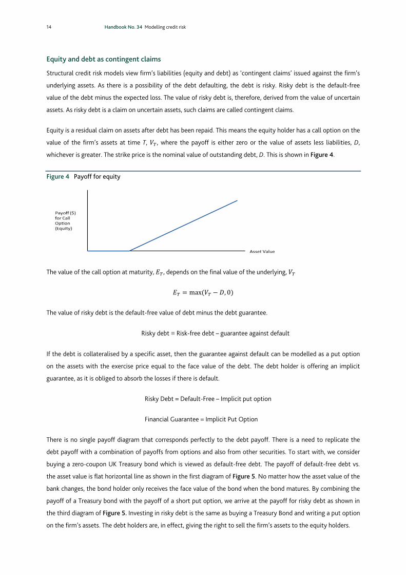
Equity is a residual claim on assets after debt has been repaid. This means the equity holder has a call option on the

value of the firm’s assets at time T, , where the payoff is either zero or the value of assets less liabilities, D,

whichever is greater. The strike price is the nominal value of outstanding debt, D. This is shown in Figure 4.

Figure 4 Payoff for equity

The value of the call option at maturity, , depends on the final value of the underlying,

max , 0

The value of risky debt is the default-free value of debt minus the debt guarantee.

Risky debt ≡ Risk-free debt – guarantee against default

If the debt is collateralised by a specific asset, then the guarantee against default can be modelled as a put option

on the assets with the exercise price equal to the face value of the debt. The debt holder is offering an implicit

guarantee, as it is obliged to absorb the losses if there is default.

Risky Debt = Default-Free – Implicit put option

Financial Guarantee = Implicit Put Option

There is no single payoff diagram that corresponds perfectly to the debt payoff. There is a need to replicate the

debt payoff with a combination of payoffs from options and also from other securities. To start with, we consider

buying a zero-coupon UK Treasury bond which is viewed as default-free debt. The payoff of default-free debt vs.

the asset value is flat horizontal line as shown in the first diagram of Figure 5. No matter how the asset value of the

bank changes, the bond holder only receives the face value of the bond when the bond matures. By combining the

payoff of a Treasury bond with the payoff of a short put option, we arrive at the payoff for risky debt as shown in

the third diagram of Figure 5. Investing in risky debt is the same as buying a Treasury Bond and writing a put option

on the firm’s assets. The debt holders are, in effect, giving the right to sell the firm’s assets to the equity holders.

boe490482

Text Box


Figure 5 Payoff diagrams for risky debt – default-free debt plus short put option

Financial crises have caused equity holders and debt holders of a bank to become more uncertain about how the

value of the bank’s assets will evolve in the future. A bank’s creditors participate in the downside risk but receive a

maximum payoff equal to the face value of debt. Equity holders benefit from upside outcomes where default does

not occur but have limited liability on the downside. So uncertainty in a bank’s asset value has an asymmetric effect

on the market value of debt and equity. The asymmetry in the payoffs to debt holders and equity holders is shown

in Figure 6.

Figure 6 Payoff to debt and equity holders of the firm

Asset value uncertainty

The central idea behind CCA is that an institution’s risk of default is driven by the uncertainty in its assets values

relative to promised payments on its debt obligations. Assets of a bank are uncertain and change due to factors

such as profit flows and risk exposures. Default risk over a given horizon is driven by uncertain changes in future

asset values relative to promised payments on debt – where these payments are often referred to as “default

barriers”. Having identified the nature of the payoffs to debt and equity holders, the next step would be to examine

how the value of a bank’s assets would evolve through time relative to a default barrier. Stochastic assets which

evolve relative to a distress barrier can be used to determine the value of liabilities with implicit options. The

probability that the assets will be below the distress barrier is the probability of default, which is required to be

estimated in order to quantify credit risk.

boe490482

Text Box


A stochastic process is a random process indexed by time. Let be the value of assets at time t. Changes in

between any two points in time can be accounted for by a certain component (the drift term) and an uncertain

component (the random or stochastic term). The drift represents the expected (average) growth rate of the asset

value. The stochastic term is a random walk where the variance is proportional to time and the standard deviation

is proportional to the square root of time. It represents the uncertainty about asset value evolution.

The dynamics of assets which are uncertain follow this “diffusion” process, with drift and volatility, given by

Such a process in continuous time is a Geometric Brownian Motion (GBM) and dz is a Wiener-process, which is

normally distributed with zero mean and unit variance. A more rigorous description can be found in Baz and Chacko

(2004).

For a GBM the asset value at time t can be calculated from the asset value at time 0 using the following

relationship:

exp √ ]

Here is the realisation of a normal random variable with mean zero and unit variance. The drift term is adjusted

by the term, , which must be included if there is uncertainty in the evolution of the assets. In a certain world,

0 and, in this case, exp .

The asset at time t may be above or below a barrier , which represents the level of promised payments on the

debt. Since assets can fall below the barrier, we can calculate the probability that .

Using the equation above for ,

exp2

√

Rearranging the probability that assets are less than or equal to the barrier is equivalent to the probability that the

random component of the asset return, , is less than :

The term is called the “distance to default” and is the number of standard deviations the current asset value is

away from the default barrier, . It is a concept pioneered by KMV Corporation and is explained in Kealhofer

(2003). Since ~ 0,1 is normally distributed,

~ ,

i.e. the probability of default on the debt is the standard cumulative normal distribution of the minus distance to

default, . Figure 7 illustrates two possible paths of the firm’s asset value. A higher asset return raises the firm’s

asset value more quickly, reducing the probability of default, other things being equal. But there is also uncertainty

boe490482

Text Box


about the asset value growth. Uncertainty about the asset value growth means that the range of possible values for

the firm’s assets widens out over time. The probability distribution of the asset value at time T is developed on the

assumption that financial assets follow a lognormal distribution. Therefore, the logarithm of the asset value follows

a normal distribution at time T. If the firm’s asset value falls below the horizontal line (default boundary), there is a

default. The probability of default is the area below the default barrier in Figure 7. In order to arrive at the

probability of default we need to estimate the mean and variance of the probability distribution.

Figure 7 Probability of default

Estimating the probability of default

Figure 8 shows a balance sheet identity that always holds: assets equal the value of risky debt plus equity. Asset

value is stochastic and may fall below the value of outstanding liabilities which constitute the bankruptcy level

(“default barrier”) D. D is defined as the present value of promised payments on debt discounted at the risk-free

rate.

Figure 8 Balance sheet evolution

boe490482

Text Box


The firm’s outstanding liabilities constitute the bankruptcy level whose standard normal density defines the

“distance to default” relative to firm value. Equity value is the value of an implicit call option on the assets with an

exercise price equal to the default barrier. The equity value can be computed as the value of a call option as shown

in equation 2.1

Equation 2.1

Where the factors and are given by

ln 2

√

√ln 2

√

Where r is the risk-free rate, σ is the asset value volatility, and N(d) is the probability of the standard normal

density function below d.

The present value of market-implied expected losses associated with outstanding liabilities can be valued as an

implicit put option, which is calculated with the default threshold D as strike price on the asset value V. The

implicit put option is given by:

Equation 2.2

The value of risky debt, B, is thus the default-free value minus the expected loss, as given by the implicit put option:

Equation 2.3

The market value of assets of banks cannot be observed directly but it can be implied using financial asset prices.

From the observed prices and volatilities of market-traded securities, it is possible to estimate the implied values

and volatilities of the underlying assets in banks. Using numerical techniques, asset and asset volatility can also be

estimated directly to calibrate the Merton model. In equation 2.1 neither V, nor is directly are directly

observable. However, if the company is publicly traded then we observe E. This means equation 2.1 provides one

condition that must be satisfied by and . can also be estimated from historical data. In order to calibrate

the Merton model we need to find a second equation in these two unknowns, and . To do so we invoke Ito’s

lemma as follows:

12

Using Ito’s lemma we can also state that:

boe490482

Text Box


Where / is the delta of the equity. It can be proved that this delta is:

Crucially, from the above we can relate the unknown volatility of asset values to the observable volatility of equity:

Equation 2.4

This provides another equation that must be satisfied by and .

Therefore, calibrating the Merton model requires knowledge about the value of equity, E, the volatility of equity,

, and the distress barrier as inputs into equations and , in

order to calculate the implied asset value and implied asset volatility .

Applying the Merton model

We illustrate the Merton model framework, described above, with an example. To do so, we initialise the

parameters of the Merton model with the following values:

V = 100; Asset value

D = 90; Default-free value of debt or “default barrier”

r = 0.05 (5%); Risk-free rate of interest

σv = 0.10 (10%); Asset value return uncertainty

T = 1; Time to maturity

The solution of the model provides throws up the value of equity, E, and the risky debt B. Using an iterative

procedure, the output of the Merton model gives value of E and B as 14.63 and 85.37 respectively. The risk-neutral

probability, that the firm will default on its debt, is N(-d2). The risk-neutral probability of default describes the

likelihood that a firm will default if the firm was active in a risk-neutral economy, an economy where investors do

not command a premium for bearing default risk.

The risk-neutral default probability N(-d2) is 6.63% for one year.

As we are modelling credit risk, we want to estimate the credit spread s. This is the risk premium required to

compensate for the expected loss (EL). The credit spread s, is the spread of the yield-to-maturity, y, over the risk-

free rate of interest, r.

The yield-to-maturity for risky debt B, denoted as y, is derived as follows;

ln

0.0028

boe490482

Text Box


Thus, credit spread for risky debt is equal to 28 basis points (0.28 per cent). For extensions of this approach to

estimate sovereign credit risk see Gray et al. (2008).

Figure 9 Variation of default probability with asset uncertainty

Using the same model parameters we can do some sensitivity analysis by varying the asset value uncertainty from

0 to 30 per cent. Figure 9 shows how the default probability increases as the volatility in asset value increases. This

implies that if the value of the bank’s assets fluctuates over time, the likelihood that the asset value will fall below

the debt value at maturity increases.

The CCA framework is useful because it provides forward-looking default probabilities which take into account both

leverage levels and market participants’ views on credit quality. In the context of stress testing, it provides a

standardised benchmark of credit risk (default probabilities) that facilitates cross-sector and cross-density

comparisons. However, CCA can only be applied to entities with either publicly traded equity or very liquid CDS

spreads, and it cannot capture liquidity or funding roll-over risk.

3. Reduced form models

In the structural credit risk model, the underlying asset value follows a standard GBM with no jumps and constant

drift and volatility:

As discussed above, this is the asset value diffusion process in the Merton (1974) model. A stochastic variable can

follow a GBM as described above and exhibit, on top of this, jumps at random times when it drops to a lower value.

From these post-jump values it can proceed with the original diffusion process till the next jump occurs and so on.

boe490482

Text Box


We can extend the equation by adding a jump process:

1

The occurrence of the jump is modelled using a Poisson process with intensity :

is a jump process defined by

with probabilities

the jump size J is drawn randomly from a distribution with probability density function P(J), say, which is

independent of both the Brownian motion and Poisson process. Intuitively, if there is a jump (dY = 1), V

immediately assumes value JV. For example, a sudden 10% fall in the asset price could be modelled by setting J =

0.9.

In the structural approach, the term is absent; the value of the firm is modelled as a continuous process, with

default occurring when the value reaches some barrier. In reduced form models, the emphasis is on the jump

process, , and default will occur at the first jump of J.

Default intensity

In reduced form, or default intensity models, the fundamental modelling tool is the Poisson process, and we begin

by demonstrating its properties. We assume there are constant draws from the Poisson distribution, and each draw

brings up either a 0 or a 1. Most of the draws come up with 0. But when the draw throws up a 1, it represents a

default. Poisson distribution specifies that the time between the occurrence of this particular event and the

previous occurrence of the same event has an exponential distribution. Box 2 formalises the Poisson process.

!

Box 2 Poisson process and distributions

A Poisson process is an ‘arrival’ process in which Nt is the number of arrivals from time 0 to time t, and,

All arrivals are of size 1.

For all t, s > 0, is independent of the history up to t.

For all t, s > 0, is independent of t.

The probability of k arrivals at time t has a Poisson distribution:

And the expected number of arrivals between 0 and t is

It is important to note that has a time dimension. For example, if it refers to a year, then t = 1, above gives the

expected arrivals in a year; t = 1/52 gives the expected arrivals in a week.

boe490482

Text Box


When the Poisson process is used for credit risk, the arrival rate is referred to as default intensity and is normally

represented by, .

The probability of default between 0 and t is

1

The probability of no default between 0 and t is

The expected time until default (i.e. the first and only possible default) is

1

Contingent convertible capital Instruments

We will apply the default intensity model, described above, for pricing contingent convertible capital instruments

(CoCos). A CoCo is a bond that will get converted into equity or suffer a write-down of its face value as soon as

the capital of the issuing bank falls below a certain trigger level. This trigger level is the point at which the bank is

deemed to have insufficient regulatory capital. A key lesson of the financial crisis has been that regulatory capital

instruments in the future must be able to absorb losses in order to help banks remain ‘going concerns.’ Triggering

the conversion of the bond into shares or activating the write-down of the face value takes place when the bank is

still a going concern. Conversion should occur ahead of banks having to write down assets and well ahead of the

triggering of resolution measures. A trigger event is a barrier that causes another event, in this case the CoCo

conversion. The risk of conversion should be compared to a default risk.

A CoCo can convert into a predefined number of shares. Another possibility is that the face value of the debt is

written down. This analysis focusses on the conversion of a CoCo into shares and the notion of a recovery rate. For

1

0

The expected waiting time ( ) until the first arrival is

and the probability of no arrivals between 0 and t is

The same parameter, , determines all the above magnitudes: it gives us the waiting times and the expected number

of arrivals by a given time. has various names including the ‘hazard rate’, the ‘arrival rate’, or the ‘arrival intensity’.

The arrivals can be used to represent the arrival of defaults in a portfolio of bonds, for example.

boe490482

Text Box


a discussion on the design characteristics of CoCos see Haldane (2011). Further quantitative analysis can be found

in Spiegeleer and Schoutens (2011).

The number of shares received per converted bond is the conversion ratio . The conversion price of a CoCo

with face value F is the implied purchase price of the underlying shares on the trigger event:

Equation 3.1

If the bond is converted into shares, the loss for the investor depends on the conversion ratio and the

value ∗ of the shares when the trigger materialises. So if the CoCo gets triggered and a conversion occurs:

Equation 3.2 ∗ 1∗

1

Equation 3.2 has brought forth the introduction of a recovery rate for a CoCo bond. Then, with the notation as

above, the recovery rate is defined as:

Equation 3.3 ∗

The recovery rate, , will be determined by the conversion price, , and the share price at conversion, ∗. The

closer the conversion price matches the market price of the shares ∗ at the trigger date, the higher this

recovery ratio.

Pricing CoCo bonds

There are alternative approaches to pricing Coco bonds. In this analysis, we view the CoCo bond as a credit

instrument and adopt a reduced form approach for pricing. It was explained in the beginning of this chapter that in

the reduced form approach, a default intensity parameter is used when modelling default. This is also known as

credit derivatives pricing. Credit instruments are usually quoted by their credit spread over the risk-free rate of

interest. The credit spread is linked to the recovery rate 1 and default intensity by what is known as the

credit triangle:

Equation 3.4 1

The credit spread is the product of the loss 1 and the instantaneous probability of this loss taking place .

Applying this principle enables one to view the trigger event whereby a CoCo is converted into shares as an extreme

event akin to that in the credit default swap market. Triggering the CoCo conversion can then be modelled as such

an extreme event. The default intensity is replaced by a trigger intensity , which has a higher value than the

corresponding default intensity. From equation 3.4 we can determine the value of the credit spread on a CoCo

using the credit triangle.

Equation 3.5 1

boe490482

Text Box


This approach can be applied to the pricing of CoCos after making some adjustments. First, to prevent the bank

from defaulting the CoCo conversion has to occur before the default time. This implies that the default intensity of

the conversion, has to be greater than the default intensity of the entity itself, namely, the bank. This is

because the CoCo will fulfil its purpose if it converts before the bank defaults.

The trigger intensity, , is linked to the probability of hitting the trigger, , according to the Poisson process:

Equation 3.6 1

where T is the maturity of the CoCo bond. The probability of hitting the trigger would be equivalent to hitting a

barrier in a barrier option framework. Equation 3.6 gives the probability of the CoCo defaulting at time T. By

solving equation 3.6 for , we get the following:

Equation 3.7

Thus equation 3.5 for the credit spread of the CoCo has the following computable solution:

Equation 3.8 1

1∗

CoCos are difficult to price because of their sensitivity to the probability of trigger. Spiegeleer and Schoutens

(2011) show that in a Black-Scholes framework, the probability ∗, of hitting ∗ is given by:

Equation 3.9 ∗

∗

√

∗∗

√

Continuous dividend yield

r = Continuous interest rate

Volatility

T = Maturity of the contingent convertible

Current share price

This allows for a closed form solution and also promotes a better appreciation of the loss absorption qualities of a

CoCo bond.

4. Counterparty credit risk

Counterparty credit risk (CCR) is the risk that the counterparty, in a transaction, defaults before settlement of final

cash flows. It exists in OTC derivatives, securities financing transactions and long settlement transactions. CCR has

the following general characteristics:

it is bilateral (that is, each counterparty can have exposure to the other)

what is known today is only the current exposure

boe490482

Text Box


it is random and depends on potential future exposure

These characteristics differentiate CCR from credit risk. Unlike market risk, CCR arises when the market value of

transactions is in your favour (that is, positive mark-to-market value) and the counterparty defaults. Quantifying

CCR typically involves:

Simulating risk factors at numerous future points in time for the lifetime of the portfolio

Re-pricing positions at each time point

Aggregating positions on a path consistent basis, taking into account netting and collateral.

Figure 10 shows quantifying exposure involves striking a balance between two effects. First, uncertainty of market

variables and, therefore, risk increases the further we go out in time. Second, derivative contracts involve cash flows

that are paid over time and reduce the risk profile as the underlying securities amortise through time. For instance,

in a 5-year interest rate swap contract, maximum exposure to the dealer is unlikely to occur in the first year as

there is less uncertainty about interest rates in that period. It is also unlikely to be in the last year since most of the

swap payments will already have been made by then. It is more likely that maximum exposure will be in the middle

of the contract. An analysis of the different methods for quantifying CCR can be found in Gregory (2011).

Figure 10 Quantifying counterparty credit risk

Credit value adjustments

Credit valuation adjustment (CVA) is often mentioned in the context of market risk and CCR. It is an adjustment

banks make to the value of transactions to reflect potential future losses they may incur due to their counterparty

defaulting. CVA is the difference between the price of a credit-risky derivative and the price of a default-free

derivative to account for the expected loss from counterparty default. Banks recognise counterparty risks in

derivatives trades and make CVA adjustments. Basel II reports that two-thirds of credit risk losses during the global

financial crisis are caused by CVA volatility rather than actual defaults. CVA is also an integral part of the Basel III

accord. However, CVA is primarily a valuation and mark-to-market pricing concept and is not a substitute for

traditional counterparty credit risk management.

boe490482

Text Box


In the presence of counterparty credit risk, the value of a derivative can be written as

Equation 4.1

Where is the value of the claim. is the credit-risk-free value of the asset and CVA is the credit value

adjustment that varies with counterparty creditworthiness. CVA is by definition 0. It follows from equation 4.1

that a credit-risky derivative has a lower price than a derivative without risk. This is because the buyer of the credit-

risky derivative (often referred to as the dealer) lowers the price of the derivative since he or she accounts for the

credit risk of the counterparty (the derivatives seller). In particular, if the counterparty defaults, the buyer of the

derivative will not receive a payout of the derivative. CVA is an adjustment since the derivatives buyer adjusts

(lowers) the price of the derivative due to credit risk.

The CVA is given by:

Equation 4.2 ∑

where

LGD is the loss given default

DFt is the discount factor for tenor t

EEt is the expected exposure at time t.

PDt is the (conditional) probability of default at time t

The value of the CVA is an increasing function of both the probability of the counterparty defaulting, as well as

expected exposure at the time of default. It can be seen from equation 4.2 that a higher PD, a higher LGD and a

higher EE would all increase the CVA. Banks’ CVA increased dramatically during the financial crisis. Regulatory

reforms focussed on reducing the magnitude of the CVA. The starting point would be to reduce the probability of

default of banks or reduce the expected exposures.

Expected exposures with and without margins

is the expected ‘in the money’ value of the contract. If a counterparty is ‘in the money’ in a derivatives

contract, 0

If there are no margins, then:

Equation 4.3 Ε , 0

Equation 4.3 shows the uncollateralised exposure. This is the expected exposure when no collateral is exchanged.

If we introduce variation margins (VM) which are calculated daily (or intraday) and marked to market, the expected

exposure (EE) diminishes. Counterparties in a derivatives transaction exchange gains and losses in this manner.

If there are daily variation margins (VM)

Equation 4.4 Ε , 0 ,

boe490482

Text Box


where , 0

VM is based on the value of the contract in the previous day. For the counterparty that is ‘in the money’, is

positive. Variations margins are designed to ensure the expected exposure never becomes too large.

Initial margins (IM) are set to cover potential losses on in-the-money derivative contracts in the event of

counterparty default. Their levels are based on a model looking at the product and historic market moves. In the

case of bilateral transactions, both parties pay and the margins are segregated. If they are centrally cleared, all

clearing members pay into a central CCP pool.

With daily variation margin (VM) and initial margin (IM)

Equation 4.5 Ε , 0 ,

where IM is set to n-day VaR, i.e. Ρ Χ 1 , and we assume m-day margin period of risk.

If there is counterparty default, the contract will have to be replaced in the market. Due to fluctuations in market

liquidity it won’t always be possible to replace the contract immediately following default. The n-day VaR is based

on the number of days it would take to do so. The m-day margin period of risk would imply that the counterparty is

exposed to the fluctuating value of the contract m-days into the future. The IM is meant to mitigate this loss.

Suppose that it may take up to 5 days to find a new counterparty to the contract and that under normal market

conditions the price should not be expected to move by more than £5 within five days with probability 99%. Then

if the initial margin is set at £5, a dealer will be protected against default of a counterparty with 99% confidence. A

95% VaR would imply that in 95 out of 100 cases, the counterparty will have enough margin to cover this loss. In

actual practice, the confidence interval is typically 99.7%.

Collateralising over-the-counter (OTC) derivatives in the bilateral market has historically been discretionary. The

2007-2009 financial crisis saw the emergence of large bilateral exposures many of which were not sufficiently

collateralised. A proliferation of redundant overlapping contracts exacerbated counterparty credit risk. Since then,

collateral has assumed a central role in OTC derivatives transactions for mitigating counterparty credit risk. To

make the OTC derivatives market more robust, the G20 has mandated that all standardised contracts be cleared

through central counterparties (CCPs) and that standards be developed for margining non-centrally cleared trades.

Stricter margin requirements for bilaterally cleared trades will also improve risk management. However, mandating

central clearing of OTC derivatives and other proposed regulatory reforms, such as Basel III, is expected to increase

demand for collateral overall. Sidanus and Zikes (2012) have made an assessment of how OTC derivatives reform

will increase the demand for high-quality assets to use as collateral.

boe490482

Text Box


References

Basel Committee on Banking Supervision (BCBS) (2005), ‘An explanatory note on the Basel II IRB risk weight

functions’, July.

BCBS (2006), Basel II: International Convergence of Capital Measurement and Capital standards: A Revised

Framework – Comprehensive Version, Bank of International Settlements, June.

BCBS (2010), ‘Calibrating regulatory minimum capital requirements and capital buffers: a top-down approach’,

October.

Baz, J and Chacko, G, (2004), ‘Financial Derivatives’, Cambridge University Press.

Durbin, J and Koopman, SJ, (2012), ‘Time series analysis by state space methods’, Oxford University Press.

Gordy, M.B. (2003), ‘A risk-factor based model foundation for ratings-based bank capital rule.’ Journal of Financial

Intermediation, 12, 199-232.

Gray, D, Merton, R, Bodie (2008), ‘A New Framework for Measuring and Managing Macrofinancial risk and

Financial Stability’, Harvard Business School Working Paper No. 9/15.

Gregory, J, (2011),‘Counterparty credit risk: the new challenge for global financial markets’, John Wiley & sons.

Haldane, A, (2011), ‘Capital Discipline. Speech given at the American Economic Association, ‘ Denver, 9 January

2011.

Haldane, A, Hall, S and Pezzini, S, (2007), ‘ A new approach to assessing risks to financial stability’, Bank of

England, Financial Stability Paper No.2.

Harvey, AC, (1989), ’Forecasting, Structural Time Series Models and the Kalman Filter,’ Cambridge University

Press.

Kealhofer, S (2003), ‘Quantifying credit risk I: Default prediction.’ Financial Analysts Journal, 59(1):30-44.

Merton, RC, (1974), ‘On the pricing of corporate debt: the risk structure of interest rates,’ Journal of Finance 51,

987-1019.

Sidanus, C and Zikes, F, (2012), ‘OTC derivatives reform and collateral demand impact‘, Bank of England, Financial

Stability Paper No. 18.

Spiegeleer, Jan D and Schoutens, W, (2011), ‘Pricing CoCos; A derivatives approach.’ Department of Mathematics,

Katholieke Universiteit Leuven.

Vasicek, O, (2002), ‘Loan portfolio value’, Risk, December, pages 160-62.

boe490482

Text Box


Appendix

Estimating the unobserved state variable using the Kalman filter

The Kalman filter is a set of equations which allows an estimator to be updated once a new observation becomes

available. It first forms an optimal predictor of the unobserved state variable vector S given its previously estimated

values. These estimates for the unobserved state variables are then updated using information provided by the

observed variables.

Let be the set of m observable variables at time t. The model can be written as

(1)

~ ,

~ 0,

~ 0,1

0,1, … ,

Where is the scalar stochastic process representing the state of macro-financial conditions, is the m-

dimensional vector of factor loadings, ∅ is a diagonal m x m matrix of AR(1) coefficients, is a diagonal matrix of

MA(1) coefficients, is the autoregressive coefficient of the unobservable stochastic process , while is a

multivariate Gaussian white noise process with diagonal variance and covariance matrix and is a scalar

Gaussian white noise with unit variance.

In order to close the model we need to specify the initial conditions for the stochastic process, . Therefore, we

assume to be normally distributed with mean and variance .

The common factor at time t is obtained as the expected value of the process, . The model parameters can be

estimated by rewriting equations (1) in state space form and using the Kalman filter. An equivalent state space

representation of (1) can be obtained as

(2)

(3)

~ Θ

Equation (2) is the measurement equation that relates the observable macroeconomic and financial variables to

the unobservable state variables ( ). Equation (3) is called the state equation, and it captures the dynamics of the

latent state variable . The algorithm works in a two-step process. In the prediction step, the Kalman filter

produces estimates of the current state variables, along with the corresponding estimation uncertainty. Once the

next measurement is observed (with some noise), these estimates are updated.

boe490482

Text Box


With the model written in state space form, the estimation of the model parameters can be obtained through the

maximisation of the likelihood.

The Kalman filter enables estimation of the conditional mean, , ,…, Θ and the conditional

variance | , , … , .

The Kalman recursions that allow us to compute the common factor as the first element of the vector Θ , are

(4) Θ

(5)

(6)

(7)

(8) Θ Θ

(9)

which are iterated starting from t = 0. The matrix in (7) is referred to as the Kalman gain.

The Kalman recursions are derived from the formula of the conditional mean and conditional variance in a

multinormal distribution. A normal distribution is fully characterised by its first two moments and the exact

likelihood function is obtained as a by-product of the Kalman filter algorithm. In order to initialise the filter we need

to specify Θ and . A possible choice is to assume these parameters to be fixed and estimate them using

maximum likelihood. Assume that ∼ Θ , , where Θ and are known and let denote the set of

parameters to estimate, i.e. , , , the likelihood function can be written as

(10) ∏ |

Since

| | Θ

Θ

|

Then

∼ 0,

Therefore the value of the likelihood function can be directly computed from the Kalman recursions in equations

(4) – (9), and the maximum of log can be obtained numerically.

boe490482

Text Box


Figure 11 depicts the ‘true state’ common factor S, around which we build the macro indicators. We have

considered two macro indicators (the blue and green lines) over a scenario of 30 years. They have been simulated

from a random number series and are not based on actual data.

Figure 11 State variable and macro indicators

Figure 12 shows the estimated S, along with the ‘true state’ S. The Kalman recursive equations, (4) to (9), have

been used to compute the estimated common factor, S.

Figure 12 True and estimated state variable

boe490482

Text Box

boe490482

Text Box

modelling credit risk - home | bank of england

Documents