modelling techniques for large- eddy simulation of wall

ACTAUNIVERSITATIS

UPSALIENSISUPPSALA

2018

Digital Comprehensive Summaries of Uppsala Dissertationsfrom the Faculty of Science and Technology 1697

Modelling Techniques for Large-Eddy Simulation of Wall-BoundedTurbulent Flows

TIMOFEY MUKHA

ISSN 1651-6214ISBN 978-91-513-0394-9urn:nbn:se:uu:diva-356729

Dissertation presented at Uppsala University to be publicly examined in ITC 2446,Lägerhyddsvägen 2, Uppsala, Friday, 21 September 2018 at 10:15 for the degree of Doctor ofPhilosophy. The examination will be conducted in English. Faculty examiner: Full ProfessorHrvoje Jasak (University of Zagreb).

AbstractMukha, T. 2018. Modelling Techniques for Large-Eddy Simulation of Wall-BoundedTurbulent Flows. Digital Comprehensive Summaries of Uppsala Dissertations from theFaculty of Science and Technology 1697. 91 pp. Uppsala: Acta Universitatis Upsaliensis.ISBN 978-91-513-0394-9.

Large-eddy simulation (LES) is a highly accurate turbulence modelling approach in which awide range of spatial and temporal scales of the flow are resolved. However, LES becomesprohibitively computationally expensive when applied to wall-bounded flows at high Reynoldsnumbers, which are typical of many industrial applications. This is caused by the need to resolvevery small, yet dynamically important flow structures found in the inner region of turbulentboundary layers (TBLs). To remove the restrictive resolution requirements, coupling LES withspecial models for the flow in the inner region has been proposed. The predictive accuracy ofthis promising approach, referred to as wall-modelled LES (WMLES), requires further analysisand validation.

In this work, systematic simulation campaigns of canonical wall-bounded flows have beenconducted to support the development of a complete methodology for highly accurate WMLESon unstructured grids. Two novel algebraic wall-stress models are also proposed and shown tobe more robust and precise than the classical approaches of the same type.

For turbulence simulations, it is often challenging to provide accurate conditions at the inflowboundaries of the domain. Here, a novel methodology is proposed for generating an inflowTBL using a precursor simulation of turbulent channel flow. A procedure for determining theparameters of the precursor based on the Reynolds number of the inflow TBL is given. Theproposed method is robust and easy to implement, and its accuracy is demonstrated to be on parwith other state-of-the-art approaches.

To make the above investigations possible, several software packages have been developedin the course of the work on this thesis. This includes a Python package for post-processingthe flow simulation results, a Python package for inflow generation methods, and a library forWMLES based on the general-purpose software for computational fluid dynamics OpenFOAM.All three codes are publicly released under an open-source licence to facilitate their use by otherresearch groups.

Keywords: Wall modelling, Inflow generation, Large-eddy simulation, OpenFOAM,Computational fluid dynamics

Timofey Mukha, Department of Information Technology, Box 337, Uppsala University,SE-75105 Uppsala, Sweden.

© Timofey Mukha 2018

ISSN 1651-6214ISBN 978-91-513-0394-9urn:nbn:se:uu:diva-356729 (http://urn.kb.se/resolve?urn=urn:nbn:se:uu:diva-356729)

12

13

τw τwτw

(x, y, z)

(u, v, w)〈·〉

δ

U0

δ x

δ

U0

y = 0

δ99 y 〈u〉 = 0.99U0

θ =∫∞0

〈u〉U0

(1− 〈u〉

U0

)y

δ∗ =∫∞0

(1− 〈u〉

U0

)y

ν

x =U0x

ν, δ99 =

U0δ99ν

, θ =U0θ

ν, δ∗ =

U0δ∗

ν.

x = 0

x ≈ 106

θ = 4060

y ≤ 0.1δ99y+ ≥ 50

δ U0

ν

τwτwτw

τw

uτ =√

τw/ρδν = ν/uτ

y+ = y/δνuτ

u+ = u/uτ

≈ 0.1δy+ ≈ 50

τ = δ99uτ/ν

∼ δνδ99

y+ y/δ

〈u〉/uτ = Φ1(y+),

(U0 − 〈u〉)/uτ = Φ2(y/δ).

Φ1 Φ2

y+ ≈ 30y/δ ≈ 0.3

〈u〉+ =1

κy+ +B.

κ B

κ = 0.41 B = 5.2

y+ < 5 〈u〉+y+

〈u〉+ y+

y+ = 〈u〉+ + e−κB

[eκ〈u〉

+ − 1− κ〈u〉+ − 1

2(κ〈u〉+)2 − 1

6(κ〈u〉+)3

],

〈u〉+ =1

κ

(1 + κy+

)+ C

(1− e(−y+/B1) − y+

B1e(−y+/B2)

),

κ = 0.41 C = 7.8 B1 = 11 B2 = 3

h = 2δ

x z

Ub

Ub =1

h

∫ h

0

〈u〉 y.

Uc 〈u〉(δ)

uτ

ν δ

b =δUb

ν, c =

Ucδ

ν, τ =

uτδ

ν.

b > 1800

τ ≈ 1000

Φ1

τ ≈ 1000

ρ

∂ui

∂t+

∂uiuj

∂xj= −1

ρ

∂p

∂xi+

∂

∂xj(2νSij) ,

Sij =1

2

(∂ui

∂xj+

∂uj

∂xi

).

xi i = 1, 2, 3 ui

p νSij

p = p/ρ

∂ui

∂xi= 0.

ui = 0

p = 0

N

N ∼ 2.75

〈u〉〈p〉

u = 〈u〉 + u′

p = 〈p〉+ p′

∂〈ui〉∂xi

= 0,

∂〈ui〉∂t

+∂〈ui〉〈uj〉

∂xj= −∂〈p〉

∂xi+

∂

∂xj

(τij + 2ν〈Sij〉

),

τij = 〈ui〉〈uj〉 − 〈uiuj〉

τij

νt ν

νt

νt

δν

ρτij

φ(x, t) =

∞∫∫∫−∞

φ(ξξξ, t)G (x, ξξξ,Δ) 3ξξξ.

φ φ GΔ

G Δ

ui p

∂ui

∂xi= 0,

∂ui

∂t+

∂uiuj

∂xj= − ∂p

∂xi+

∂

∂xj

(2νSij

),

Sij =1

2

(∂ui

∂xj+

∂uj

∂xi

).

uiuj

uiuj uiuj

∂ui

∂t+

∂uiuj

∂xj= − ∂p

∂xi+

∂

∂xj

(τij + 2νSij

),

τij = uiuj − uiuj

τijτij

τij

N ∼ 1.85

τij

νν

νl t

ν ∼ l2

t= u l ,

u lΔ

k = τkk /2 k

∂k

∂t+

∂uik

∂xi= 2ν SijSij − Ce

k3/2

Δ+

∂

∂xi

(ν

∂k

∂xi

)+ ν

∂2k

∂xi∂xi,

Ce = 1.048 ν

ν = CkΔ√

k ,

Ck = 0.094

Ce Ck

Ce Ck

1/t

ν = (CsΔ)2√

2SijSij ,

Cs ≈ 0.18ν

y → 0 yν

Sij Ωij = (∂ui/∂xj −∂uj/∂xi)/2 ν ∼ y3 y → 0

Sd

ν

ν = (CwΔ)2(Sd

ijSdij)

3/2

(SijSij)5/2 + (SdijS

dij)

5/4.

ν

ν

ν

ν

φ

∂p/∂xi

∂p/∂xii i i

Δ V13

G =

{1/Δ3, ∈ V

0,

Sij ν

δ δνx η

y+ y/δ

δ δν

ui(x, η, z, t) = 〈ui〉(x, η) +Ai(x, η)ui,p(x, η, z, t),

Ai(x, η)ui,p

〈ui〉 Ai xui,p

x

ui,p

η ui,p

ui xx

〈ui〉(x , η, t)− 〈ui〉(x , η, t+Δt)

〈ui〉(x , η, t)− 〈ui〉(x , η, t+Δt)=

x − x

x − x,

ui,p

η

x

〈u〉 (y+) = γ〈u〉 (y+),

〈u〉 (η ) = γ〈u〉 (η ) + (1− γ)U0,

γ uτ, /uτ, η = y/δ

〈v〉 (y+) = 〈v〉 (y+),

〈v〉 (η ) = 〈v〉 (η ).

uτ

(u′i) (y+) = γ(u′

i) (y+),

(u′i) (η ) = γ(u′

i) (η ).

850θ

y

0 < y < bm, 0 < z < hm,

bm hm

y = 0

θ

θ

δ∗ δ99

τ

θ

θ

δ∗

δ99 τ

(bm, hm, U0, θ , ν).

θ

θ δ

U0 Uc

θ =Uc

ν

∫ δ

0

〈u〉Uc

(1− 〈u〉

Uc

)y.

b θ

b

(lp, bp, δ, Ub, νp).

(lp, bp, δ, Ub, νp)(bm, hm, U0, θ , ν)

bp = bm νp = ν θp = θ

Uc = U0

Uc

Ub= f1( θ),

f1( θ) ≈ 1 + α1−β1

θ

δ

δ

θ= f2( θ),

f2 ≈ γ2 + α2β2

θ

f1 f2

f1 f2

i αi βi γi

2.603 · 10−4

lp = 8δ

θ ≈ 830

θ ≈ 830

≈ 270θ 370θ

1.85

∼ δν

N ∼

τwτwτwh

h

x1 x3

x2

x1

∂τij/∂xj τij = τij + 2νSij

Sw

∂τij/∂xj∮τijnj S n

∫Sw

τijnj S = −∫Sw

τi2 S ≈ τw,i2Sw. (i = 1, 3)

τw,12 τw,32

τwτwτw τwτwτwτw

τwτwτw

u p

h

τw

τwτw,12 τw,32

ui

τi2

τw,i2 = (ν + ν )fui,P

Δx2. (i = 1, 3)

Pf Δx2

τwν

ν =τw[

(u1,P /Δx2)2+ (u3,P /Δx2)

2]1/2 − ν.

ui

τwτwτw

τw τw

τwτw

τwτw

τw τwτw

τ ′wτwτ ′w

δ(δ/20)2

τ = δ/δν

τw

≈ 750δν × 100δντ ′w

≈ 1500δν × 700δν(1000δν)

2

(δ/20)2 τ = 20 000τ ′w

τ ∼ 104

τ ≤ 2000

τw τw

τ = 1000 τwτw(δ/20)2

τ+w = τw/〈τw〉 τ+w = τw/〈τw〉

≈ 0.50.794

τ+w τ+w τ = 1000

τw

τw /〈τw〉 = 0.418τw

0.288τw τw

τw τw

τw∼ 104 τw

τ ′w

τw

τ ′w

τwτwh

τwu

〈u〉

τw,12 =u1|h〈u〉|h 〈τw〉,

·|h

〈u3〉〈τw,32〉

τw,12

τ ′w,12 u′1|h τ ′w,12

〈τw〉

〈u〉/√〈τw〉 − 1

κ

(x2

√〈τw〉/ν

)−B = 0.

〈u〉x2 = h

〈τw〉

〈τw〉

τ ′w〈τw〉

〈u〉|h

τ ′w〈τw〉

τ ′w〈τw〉

τ ′w

τw

τwu

u τw

τ ′wτ = 1000τw

uu

h

uτw

τ ′w

uτ

h/δ = 0.025≈ 0.62

h/δ ≈ 0.3< 0.1

τwh/δ

τw u

uτ

u∗τ u

h/δ

h/δτ ′w

τ = 1000 τw

u τw

〈τw〉

〈τw〉

∂

∂x2

[(ν + νt)

∂〈ui〉∂x2

]= Fi,

Fi =1

ρ

∂〈p〉∂xi

+∂〈ui〉∂t

+∂

∂xj〈ui〉〈uj〉.

i = 1, 3 u2

h

y = h

νt

νt

τ

0.2 0.5100 150

τw

νt

νt = νκx+2

(1− (−x+

2 /A))2

,

κ = 0.41 A = 17.8〈uτ 〉

νt

uτp = (u2τ + u2

p)1/2

up = |ν/ρ(∂p/∂x1)|1/3 α = u2τ/u

2τp

uτ uτp

x∗2 = x2〈uτp〉/ν

νt = νκx∗2

[α+ x∗

2(1− α)3/2]β [

1−(− x∗

2

1 +Aα3

)]2,

A = 17 β = 0.78

F

F = 0

〈τw〉

Fi =∂〈p〉∂xi

∣∣∣∣h

F νt

x2 = hF

x2

F

hh

hx+2 > 50

x2/δ ≈ 0.3h

h

h〈τw〉

u τw hτw

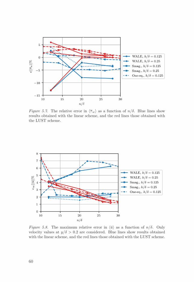
τ = 1000〈τw〉 ε[〈τw〉] h/δ

uh/δ = 0.025

u

h

ε[〈τw〉] h/δu

h/δ 〈τw〉h/δ

h/δ

u /〈u〉 uh/δ

τw

u

u u

u x2 = hh

τ = 1000〈u〉/Ub

δ/20

τ =1000

δ/20〈u〉/Ub

u

h

τ = 5200

n/δ

h/δ

〈τw〉 h/δ

〈τw〉 h/δ

h/δ ≈ 0.2 〈τw〉〈u〉

h

h

h/δ

h/δ > 0.1

〈τw〉h/δ

u|h

h

h/δ < 0.05

〈τw〉 h/δ

〈τw〉

h/δ

τ =5200

τw

n/δ10 30

〈τw〉〈u〉

〈τw〉 n/δ

h/δ 0.125 0.25

n/δ > 20

〈u〉

〈u〉 y/δ > 0.2〈u〉

n/δ = 30

〈τw〉 n/δ

〈u〉 n/δy/δ > 0.2

h〈τw〉

h τw

n/δ = 30h

δ

δ

δ

δ

≈ 0.064δ n/δ ≈ 15.5

h

h δcf

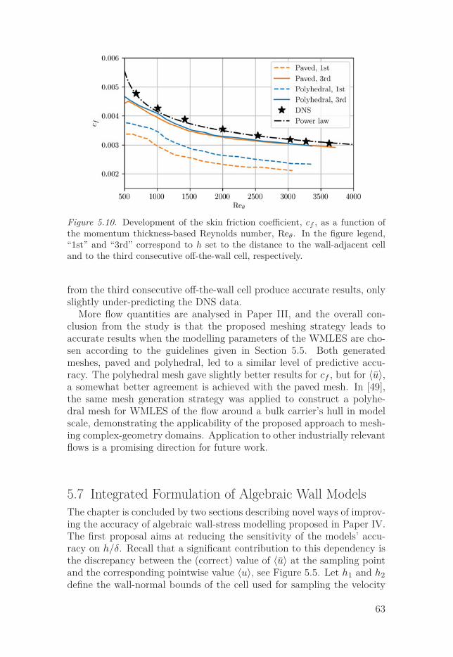
cfθ

h

cf 〈u〉

h/δ〈u〉

〈u〉 h1 h2

h = (h1+h2)/2〈τw〉〈u〉|h

〈τw〉

〈u〉|h ≈ 1

h2 − h1

∫ h2

h1

〈u〉 x2

〈u〉+ = F (〈τw〉, x+2 , q) q

F (〈τw〉, x+2 , q) x2

〈u〉|h 〈τw〉

〈u〉|h =〈uτ 〉

h2 − h1

∫ h2

h1

F (〈τw〉, x+2 , q) x2.

F (〈τw〉, x+2 , q)

h

h1

h2

u

〈τw〉u

h/δ

h/δ

τw

κ B

τw

ui i = 1 . . . n nhi/δ

u∗τ

u∗i = ui/u

∗τ h∗

i = hiu∗τ/ν

uτ

u∗i h∗

i

τw

ui

uτ

≈ 0.91ui τw

≈ 0.62h/δ = 0.025

〈u〉 k = 〈u′iu

′i〉/2

U0

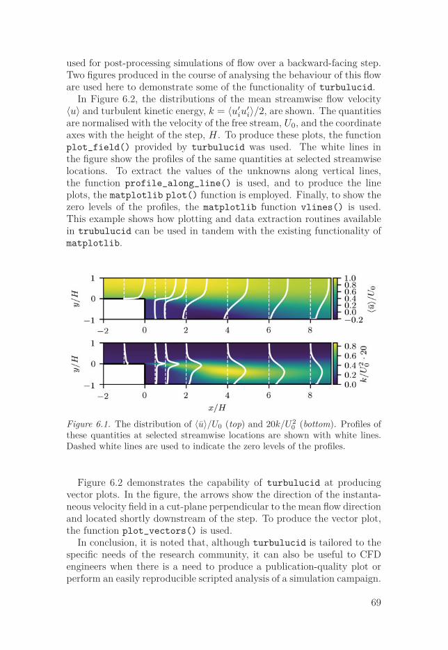
H

〈u〉/U0 20k/U20

H

τwν

F F = 0 Fi = ∂p/∂xi|hνt

h h

ν

n/δ = 30

〈τw〉〈u〉

h〈τw〉

h

τw

θ = 830 2 400

τw τwτ = 1000

h/δ n/δ

〈τw〉 h/δ

τw

u τw

〈u〉〈τw〉

∂ui

∂xi= 0,

∂ui

∂t+

∂uiuj

∂xj= −1

ρ

∂p

∂xi+ ν

∂2ui

∂xj∂xj.

xi i = 1, 2, 3 ui

p ν

h

ui = 0

τ ≈ 5200

θ = 6650

θ = 1410

Acta Universitatis UpsaliensisDigital Comprehensive Summaries of Uppsala Dissertationsfrom the Faculty of Science and Technology 1697

Editor: The Dean of the Faculty of Science and Technology

A doctoral dissertation from the Faculty of Science andTechnology, Uppsala University, is usually a summary of anumber of papers. A few copies of the complete dissertationare kept at major Swedish research libraries, while thesummary alone is distributed internationally throughthe series Digital Comprehensive Summaries of UppsalaDissertations from the Faculty of Science and Technology.(Prior to January, 2005, the series was published under thetitle “Comprehensive Summaries of Uppsala Dissertationsfrom the Faculty of Science and Technology”.)

Distribution: publications.uu.seurn:nbn:se:uu:diva-356729

ACTAUNIVERSITATIS

UPSALIENSISUPPSALA

2018

modelling techniques for large- eddy simulation of wall

Documents