Modular Forms, Elliptic Curves, and their Connectionto Fermat’s Last Theorem

Dylan Johnson

ABSTRACT

Fermat’s Last Theorem (FLT) states that if n is an integer greater than three, the equationxn + yn = zn has no integer solutions with xyz 6= 0. This incredible statement eluded prooffor over three-hundred years: in that time, mathematicians developed numerous tools whichfinally proved FLT in 1995. In this paper, we introduce some of the essential objects whichenter the proof — especially modular forms, elliptic curves, and Galois representations —with an emphasis on precisely stating the Shimura-Taniyama Conjecture and explaining howits proof finally settled FLT. We offer proofs whenever they clarify a definition or elucidatean idea, but generally prefer examples and exposition which make concrete a truly beautifulbody of mathematical theory.

i

Contents

0 Introduction 1

1 Some Algebraic Number Theory 31.1 Unique Factorisation and the Ring of Integers . . . . . . . . . . . . . . . . . 31.2 Inverse Limits and the Absolute Galois Group . . . . . . . . . . . . . . . . . 5

2 Modular Forms 82.1 The Group Action . . . . . . . . . . . . . . . . . . . . . . . . . . . . . . . . 82.2 An Early Definition and Examples . . . . . . . . . . . . . . . . . . . . . . . 112.3 Congruence Subgroups . . . . . . . . . . . . . . . . . . . . . . . . . . . . . . 12

3 Hecke Operators and Newforms 163.1 The Double Coset Operator . . . . . . . . . . . . . . . . . . . . . . . . . . . 163.2 The diamond Operator and Dirichlet Characters . . . . . . . . . . . . . . . . 173.3 The Tp Operator . . . . . . . . . . . . . . . . . . . . . . . . . . . . . . . . . 213.4 Newforms . . . . . . . . . . . . . . . . . . . . . . . . . . . . . . . . . . . . . 22

4 Elliptic Curves 264.1 Projective Space . . . . . . . . . . . . . . . . . . . . . . . . . . . . . . . . . 274.2 Elliptic Curves . . . . . . . . . . . . . . . . . . . . . . . . . . . . . . . . . . 284.3 Torsion and the Tate Module . . . . . . . . . . . . . . . . . . . . . . . . . . 314.4 Reduction of Elliptic Curves over Q . . . . . . . . . . . . . . . . . . . . . . . 33

5 Galois Representations 355.1 Frobenius Elements and Galois Representations . . . . . . . . . . . . . . . . 355.2 Galois Representation Associated to an Elliptic Curve . . . . . . . . . . . . . 385.3 Galois Representation Associated to a Newform . . . . . . . . . . . . . . . . 41

6 The Shimura-Taniyama Conjecture 43

7 Overview of the Proof of Fermat’s Last Theorem 47

References 49

ii

0 Introduction

Proven in 1995, Fermat’s Last Theorem (FLT) remains a celebrity of twentieth centurymathematics. FLT states that for n ≥ 3, the equation xn + yn = zn has no integer solutionswith xyz 6= 0. The saga of FLT began in 1637 when Pierre de Fermat — a French lawyer whoenjoyed mathematics in his spare time — conjectured his theorem in the margin of an oldmath book. Fermat wrote that he had found a “truly marvelous proof” of the theorem, butthat the book’s margin was simply “to narrow to contain it”. Because Fermat never publisheda formal proof — and it took mathematicians over three hundred years to devise one — itseems almost certain that Fermat never actually proved his own theorem. Nevertheless, hesparked a wildfire: countless mathematicians developed incredible mathematics in an effortto prove FLT.

Early attempts relied on a crucial simplifying observation: a non-trivial solution — i.e.a solution with xyz 6= 0 — to the equation xpd + ypd = zpd for the exponent pd yields anon-trivial solution (xd)p + (yd)p = (zd)p for the exponent p. Because Fermat did indeedprove his theorem in the case of n = 4, the observation shows that proving FLT for anyexponent n ≥ 3 reduces to proving FLT for equations xp + yp = zp with p an odd prime. Sothe first progress on FLT involved checking the statement for p = 3 (by Euler in 1770), p = 5(by Legendre and Dirichlet, independently, around 1825), and p = 7 (by Lame in 1865).

The first substantial case of FLT came from the work of Sophie Germain in 1823. Germainintroduced a much more general strategy for attacking the problem which ultimately splitthe problem into two cases:

1. Case 1 is the non-existence of xp + yp = zp for which p doesn’t divide xyz; and

2. Case 2 is the same but when p does divide xyz.

Together with Legendre, Germain applied her techniques to prove the first case of FLT for allprimes less than or equal to 197 (see [Rid09] for additional details). In particular, Germainshowed that the first case of FLT holds for odd “Germain primes”: an odd prime p suchthat 2p + 1 is also prime. It remains unknown whether or not there exist infinitely-manyGermain primes, so we still aren’t sure if Germain’s results gave an infinitude of results onFLT.

The next substantial case of FLT came from Ernst Kummer who drew upon ideas byLame on unique factorisation. Kummer proved (both case 1 and case 2) of FLT for so-called“regular primes” around 1850. The precise definition of a regular prime relies on the notionof factorisation of ring ideals; in section 1, we introduce some of these ideas (and defer to[Mil17] for the rest). Although certain heuristics predict that roughly 61% of primes areregular, whether or not there are infinitely-many remains a mystery. So two hundred yearsafter Fermat conjectured his theorem, mathematicians still weren’t sure about infinitelymany cases.

The twentieth century witnessed the development of a wonderful body of mathematicswhich would go on to prove Fermat’s Last Theorem. Of central importance are the ideasof Goro Shimura and Yutaka Taniyama — who conjectured a precise relationship between“modular forms” and “elliptic curves” — and Jean-Pierre Serre — who conjectured a preciserelationship between “modular forms” and “Galois representations”. Ultimately, the link

1

between modular forms and elliptic curves became an invaluable tool and by 1990 it wasknown that Fermat’s Last Theorem would follow from the Shimura-Taniyama Conjecture.Andrew Wiles thus proved FLT by proving (most of) Shimura-Taniyama.

In this paper, we offer a broad overview of the twentieth century mathematics whichproved FLT; we emphasise the role of the Shimura-Taniyama Conjecture (STC) in the proofand indeed develop the necessary language to precisely state STC. Along the way, we intro-duce some of number theory’s most important tools and techniques. While we provide manyproofs (especially in sections 2 and 5), we generally prefer illustrative examples to technicalarguments.

Section 1 introduces some essential algebraic number theory (material from [Mil17] and[Mil18]), and is intended mostly as a reference for later sections. Section 2 introduces modularforms and their relationship with subgroups of SL2(Z) (material from chapters 1 and 2 of[DS05]). Section 3 introduces Hecke operators as well as newforms, the modular forms whichplay a role in STC (material from chapter 5 of [DS05]). Section 4 introduces elliptic curves,including the Tate module of an elliptic curve and reduction of curves over Q (material fromchapters 3 and 7 of [Sil86]).

Section 5 shifts to the construction of Galois representations for both newforms and ellip-tic curves, as well as discusses the structure of the absolute Galois group Gal(Q/Q) (materialfrom chapter 8 of [Mil17] and chapter 9 of [DS05]). Finally, section 6 states the Shimura-Taniyama Conjecture and goes through an explicit example to illustrate the statement (ma-terial from chapter 9 of [DS05] and [Wes99]). Section 7 then brings everything together byoutlining the stepping stones which go into proving FLT (material from [DDT07]).

1. Some AlgebraicNumber Theory

2. Modular Forms3. Hecke Operators

and Newforms

4. Elliptic Curves

5. Galois Rep-resentations

6. The Shimura-Taniyama Conjecture

7. Overview of theProof of Fermat’s

Last Theorem

2

1 Some Algebraic Number Theory

Developed throughout the nineteenth and early twentieth century, basic algebraic numbertheory forms the foundation for not only Lame and Kummer’s early attempts at FLT, butalso for the Shimura-Taniyama Conjecture and Wiles’s ultimate proof. In this section, wehighlight the essential results we will need later, and intend that this section serves only asa reference for subsequent sections.

1.1 Unique Factorisation and the Ring of Integers

One of the greatest structural features of the integers is that they permit unique factori-sation. Indeed, a common strategy for attacking problems over Z is to first consider theproblem for irreducible (prime) integers — which are often easier to understand — beforethen assembling information for a general integer from information on its prime divisors.But unique factorisation fails in rings “not too much larger” than the integers: for example,6 = 2 · 3 = (1 +

√−5)(1 −

√−5) in Z[

√−5]. Roughly speaking, the algebraic number

theory of the late 1800s worked to recover a notion of unique factorisation in more generalrings. Ultimately, the solution is to consider factorisation of ring ideals, rather than of ringelements.

We begin with some essential algebraic notions. Throughout this section, we will workover Q — as Q is our principal concern as number theorists — keeping in mind that manyof these ideas naturally generalise to arbitrary rings/fields.

Definition 1.1. A number α ∈ C is an algebraic number if there exists a polynomial

f(x) = xn + an−1xn−1 + · · ·+ a1x+ a0, ai ∈ Q

such that f(α) = 0.

We denote by Q the set of all algebraic numbers, where the notation comes from thealgebraic closure of a field; that is, Q may equivalently be thought of as the algebraic closureof Q, just as C is the algebraic closure of R. Similarly, we define an algebraic integer byreplacing Q with Z:

Definition 1.2. A number α ∈ C is an algebraic integer if there exists a polynomial

f(x) = xn + an−1xn−1 + · · ·+ a1x+ a0, ai ∈ Z

such that f(α) = 0.

We denote by Z the set of all algebraic integers, where the notation comes from a moregeneral notion of “integral closure”. Finally, rather than consider all algebraic numbers Q,we will want to consider finite subfields.

Definition 1.3. Consider the tower of field extensions Q ⊂ K ⊂ Q. We call K an (al-gebraic) number field if it is a finite algebraic extension of Q. In this case, we callOK := K ∩ Z the ring of integers of K.

3

As hinted at in the introductory paragraph, the terminology comes from the prototypicalexample: Z is the ring of integers in Q. Indeed, let p

q∈ Q satisfy the polynomial f(x) =

xn +∑n−1

k=0 akxk. Then

f

(p

q

)=pn

qn+

n−1∑k=0

akpk

qk= 0 =⇒ pn +

n−1∑k=0

akpkqn−k = 0 =⇒ q divides p

so an integral element pq

is indeed an integer. The following two theorems summarise theresults we need.

Theorem 1.4. Let L be an algebraic number field with ring of integers OL. Then any ideala ⊂ OL uniquely factors into a unique, finite product

a =

g∏i=1

peii

with each pi a prime ideal and ei ≥ 1. Moreover, every prime ideal pi is maximal.

Theorem 1.5. Let Q ⊂ K ⊂ L be a tower of algebraic number field with ring of integersOK and OL. Further, let p denote a prime (maximal) ideal in OK and kp the field OK/kp.By the previous theorem, we have a unique factorisation

pOL =

g∏i=1

piei

into a product of prime ideals pi ⊂ OL. Then letting li be the field OL/pi and fi the index[li : kp], we have

g∑k=1

eifi = [L : K].

Moreover, if L/K is Galois, then ei = ej =: e and fi = fj =: f for all i, j; in particular,efg = [L : K].

In theorem 1.4, we have the promised result: unique factorisation of ideals. In theorem1.5, we control the way an ideal may factor when we promote it to an ideal in a larger ringof integers. Momentarily, we will give names to various types of factorisations as well asspecialise to the case when L/K is Galois. But we first return to our motivating example:Z[√−5].

Recall that 6 = 2 · 3 = (1 +√−5)(1−

√−5) represents a failure of unique factorisation

of elements in Z[√−5]. As in theorem 1.5, with K = Q, OK = Z, L = Q[

√−5], and

OK = Z[√−5], we may regard (2) and (5) — prime ideals in OK — as ideals in OL. In this

case, we obtain factorisations

(2) = (2, 1 +√−5)2

(3) = (3, 1 +√−5)(3, 1−

√−5).

4

Moreover, the ideals (1 +√−5), (1−

√−5) ⊂ OL factor as

(1 +√−5) = (2, 1 +

√−5)(3, 1 +

√−5)

(1−√−5) = (2, 1 +

√−5)(3, 1−

√−5)

so we obtain a completely unique factorisation of the ideal (6) ⊂ Z[√−5]:

(6) = (2, 1 +√−5)2(3, 1 +

√−5)(3, 1−

√−5).

In this example, we appealed to an extremely crucial case of the theorem 1.5: when K = Qand L is some number field. We will almost exclusively consider this case.

Now, we enumerate various types of factorisations:

Definition 1.6. Use the setup as in theorem 1.5. If g = 1 and ei = 1, then we have

pOL = p1

so p remains prime in OL and we say that p is inert. If g = [L : K] — so that ei = 1 = fifor all i — then we have

pOL =

g∏i=1

pi

and we say that p splits (or splits completely). Finally, if there is some j such that ej > 1,we say that p ramifies in OL. In all cases, we say that the primes pi divide p — or thatthe primes pi lie above p — and naturally denote this by pi|p.

So for L = Q[√−5] the number field from before, we see that the ideal (2) ramifies in L

while the ideal (3) splits completely. Contrast this with the situation for Z[i], the ring ofintegers in L = Q[i]. In this case, (2) = (2, 1 + i)2 is the only prime to ramify, while (3)remains inert and (5) = (5, 2+ i)(5, 2− i) splits completely. In particular, (5, 2+ i) lies above(5) in Q[i].

For our purposes, ramification will be the case of greatest interest, owing in large part tothe rarity of ramification:

Theorem 1.7. Use the setup as in theorem 1.5. Let R(OL) = {p ⊂ OK : p ramifies in OL}.Then R(OL) is finite; succinctly, only finitely-many primes ramify.

For our favourite example L = Q[√−5] over Q, we’ve previously seen that (2) ramifies;

the only other prime to ramify is (5) = (5,√−5)2. In fact, for any square-free integer D,

the quadratic extension Q[√D] has ramification exclusively at the primes dividing D and

sometimes at (2).

1.2 Inverse Limits and the Absolute Galois Group

Recall that a field extension L/K is Galois if the extension is both normal — every irreduciblepolynomial over K either (i) remains irreducible over L or (ii) splits completely over L —and separable — every minimal polynomial over K of an element of L is separable. Inparticular, a field of characteristic zero is automatically separable, so a characteristic-zerofield extension L/K is Galois if it is normal. It follows that the extension Q/Q is Galois, soit makes sense to speak of the extension’s Galois group.

5

Definition 1.8. The group GQ := Gal(Q/Q) := Aut(Q/Q) is called the absolute Galoisgroup (of Q).

We will realise the absolute Galois group as a natural limit of finite-degree Galois groups.Along the way, we’ll define a construction called the inverse limit, a fundamental techniquein mathematics and especially useful for defining a number of objects we’ll need later.

Consider the tower of field extensions Q/L/Q with L/Q a Galois number field. Thenthere is a natural surjection GQ → Gal(L/Q) given by restriction: for any σ ∈ GQ, defineσL ∈ Gal(L/Q) by σL := σ|L. Conversely, given all such σL, we can reconstruct σ: for anys ∈ Q, pick a Galois number field L such that s ∈ L so that σ(s) must be σL(s). We thushave a natural pairing between elements of σ ∈ GQ and collections {σLi

}i∈I — where I is anindex set and Li ranges over the Galois number fields Li/Q — such that

• for all i and j, the automorphism σLi∈ Gal(Li/Q), and σLj

= σLjon Li ∩ Lj; and

• the automorphism σ restricts to σLion Li.

The first bullet is a sort of “compatibility” requirement which forces automorphisms indistinct Galois groups to knit together in a natural way. The second bullet connects elementsof the massive Galois group GQ to elements of “small”, finite extensions. This is a specialcase of the following construction.

Definition 1.9. Let (I,≤) be a directed partially-ordered set. Let {Gi}i∈I be a collectionof groups with maps rj,i : Gj → Gi such that rj,i ◦ rk,j = rk,i for all k ≥ j ≥ i. The pair(Gi)i∈I and (rj,i)i,j∈I make up an inverse system of groups and bonding morphisms over I.

Definition 1.10. The inverse limit of an inverse system (Gi)i∈I and (rj,i)i,j∈I is definedby

lim←−i∈I

Gi =

{(ai) ∈

∏i∈I

Gi : rj,i(aj) = ai for all j ≥ i

},

a subgroup of the direct product∏

i∈I Gi. The condition that rj,i(aj) = ai is called thecompatibility condition of the system as it ensures that the elements of the inverse systemare compatible with the reduction maps. If each Gi has a topology, then we endow lim←−i∈I Gi

with the subspace topology of the product topology on∏

i∈I Gi.

Let’s apply this definition to our motivating example GQ. In this case, our partiallyordered set is the set {Li}i∈I of all Galois number fields Li/Q with an ordering ≤ given by

Li ≤ Lj ⇐⇒ Li ⊂ Lj.

Further, set Gi := Gal(Li/Q) and for Lj ≥ Li define the bonding morphism rj,i : Lj → Liby restriction. Then any Lk ≥ Lj ≥ Li satisfy rj,i ◦ rk,j = rk,i and we indeed have an inversesystem. The following diagram shows an excerpt of this massive inverse system, where thenotation Gal(L) denotes the Galois group Gal(L/Q) for various number fields L.

6

. . .... . .

.. .. . . .

... . .. . . .

... . ..

Gal(Q(√

2,√

3)) Gal(Q(√

2,√

5)) Gal(Q(e2πi/5))

Gal(Q(cos(2π7

)))

. . .... . .

.

Gal(Q(√

2)) Gal(Q(√

3)) Gal(Q(√

5)) · · ·

Gal(Q)

The earlier discussion (together with Zorn’s Lemma if we want to be entirely formal) justifiesthat

GQ ∼= lim←−i∈I

Gal(Li/Q)

so, as promised, we have realised GQ as a limit of finite Galois groups. Momentarily, we willdiscuss the topology this yields. But we first discuss another essential example.

Example 1.11. Let I denote the set of positive integers with their natural ordering and fix` an integer prime. For n ∈ I, set Gn := Z/`nZ and for n ≥ m define rn,m : Z/`nZ→ Z/`mZby reduction mod `m. Then we have an inverse system

Z/`Z← Z/`2Z← Z/`3Z← · · · ← Z/`nZ← · · ·

where all maps are given by reduction mod some power of `. But this time we get an objectwe have not yet encountered:

Z` := lim←−n∈I

Z/`nZ.

An important structural feature of Z` is that we have an embedding Z ↪→ Z`: send aninteger a to the sequence (a, a, a, a, a, . . . ) where nth entry “a” denotes the reduction of amod `n. The sequence is in Z` because we certainly have the compatibility condition

rm,n(a mod `m) = a mod `n

for all m ≥ n. Moreover, the map is injective because an integer a such that a ≡ 0 mod `n

for all n must itself equal 0. So we indeed have a (canonical) embedding of Z into Z`.For an example of a non-integer element of Z`, consider the sequence (a1, a2, a3, a4, . . . )

given byan = 1 + `+ · · ·+ `n−1

so that a1 = 1, a2 = 1 + `, a3 = 1 + ` + `2, and so forth. For n ≥ m, reducing an mod `m

yields am so once again the sequence satisfies the compatibility condition and is in Z`. For` > 2, the sequence does not represent an integer because it never stabilises (when ` = 2,the sequence represents -1 under the aforementioned embedding Z ↪→ Z`).

7

Definition 1.12. The object Z` constructed in the preceding example is the ring of `-adicintegers. Its field of fractions is Q`, the field of `-adic numbers. As the names suggest,Z` is in fact the ring of integers inside Q`.

If we endow each finite Galois group Gal(Li/Q) with the discrete topology, for Li a Galoisnumber field, then the inverse limit lim←−i Gal(Li/Q) equips GQ with its own topology. Wecall this topology the Krull topology on GQ and for our purposes we only need a particularlyimportant collection of open subgroups in GQ.

Definition 1.13. Let X be a topological space and fix x ∈ X. A neighbourhood baseN for x is a set of (open) neighbourhoods of x such that any neighborhood U of x containssome N ∈ N .

Theorem 1.14. In the Krull topology on GQ, the collection

{Gal(Q/M) : M/Q finite and Galois}

constitutes a neighbourhood base of the identity. In particular, the subgroups Gal(Q/M) areopen for M/Q finite and Galois.

Our ultimate goal is to associate to “elliptic curves” and “modular forms” certain contin-uous maps GQ → GL2(Q`). Continuity will be determined with respect to the Krull topologyon GQ and the subgroups in theorem 1.14 will figure prominently. But before we do any ofthat we must first define both modular forms (section 2) and elliptic curves (section 4).

2 Modular Forms

Broadly speaking, modular forms are functions on the upper-half of the complex plane whichare holomorphic and exhibit significant symmetry. To make precise this notion of symmetry,we’ll study an important group action before then linking the group action to modular forms.

2.1 The Group Action

We begin by defining an essential group action, which appears not only in the theory ofmodular forms, but also in complex analysis, hyperbolic geometry, geometric group theory,the theory of continued fractions, and elsewhere. Our acting group will be SL2(Z), the groupof 2 by 2 integer matrices with determinant one:

SL2(Z) =

{(a bc d

): a, b, c, d ∈ Z, ad− bc = 1

}.

In the context of modular forms, we will often refer to SL2(Z) as the “modular group”. Ourset on which the modular group will act is H∗ := H∪Q∪{∞}: the upper-half of the complexplane,

H = {z ∈ C : Im(z) > 0} ,

together with its “rational limits”, the points Q and infinity.

8

In words, we will refer to H∗ as the “extended upper-half-plane”. To distinguish elementsof H, we will always use τ to denote a complex number with positive imaginary part (unlessotherwise specified); similarly, we will always use s to denote a point of Q∪{∞} and use γ todenote a matrix in SL2(Z). The action takes place as follows: a matrix γ = ( a bc d ) ∈ SL2(Z)acts on H by taking τ to

γ(τ) :=aτ + b

cτ + d. (1)

Because

Im(γ(τ)) =Im(τ)

|cτ + d|2,

that the Im(τ) is greater than 0 implies that Im(γ(τ)) > 0. So the action indeed sendselements of H to elements of H. Analogously, a matrix γ = ( a bc d ) ∈ SL2(Z) acts on Q∪{∞}by taking s to

γ(s) :=aτ + s

cs+ d.

In particular,∞ maps to the rational number ac

unless c = 0, in which case∞ maps to itself.Similarly, a number s ∈ Q maps to another rational number unless cs+ d = 0, in which cases maps to ∞. This shows that the action of SL2(Z) not only shuffles around the points ofH, but also shuffles around the rational limits Q ∪ {∞}.

Notice that for all z ∈ H∗, the identity I := ( 1 00 1 ) satisfies I(z) = z. Thus, for z 7→ γ(z)

to define a group action, one need only check that γ1(γ2(z)) = (γ1γ2)(z). Our main objectiveis to define and study “modular forms”, holomorphic functions which play nicely with theaction of SL2(Z) on H∗. But first we study the action of the modular group in its own rightfor which we introduce an incredible lemma regarding the structure of SL2(Z).

Lemma 2.1. The modular group SL2(Z) is generated by the matrices

(1 10 1

)and

(0 −11 0

).

Proof. Take ( a bc d ) ∈ SL2(Z) and let S denote the group of matrices generated by ( 1 10 1 ) and

( 0 −11 0 ); we will exhibit a sequence of matrices in S which, by right multiplication, take ( a bc d )

to a matrix in S. This will prove that SL2(Z) ⊂ S; because S ⊂ SL2(Z) automatically, theclaim will follow.

Now, note that ( 1 10 1 )n = ( 1 n

0 1 ) ∈ S. Computing(a bc d

)(1 n0 1

)=

(a an+ bc cn+ d

)(2)

and (a bc d

)(0 −11 0

)=

(b −ad −c

)(3)

illustrates how the matrices in S act by right multiplication. In particular, we may choose nin equation 2 such that ( a1 b1

c1 d1) := ( a bc d )( 1 n

0 1 ) satisfies 0 ≤ |d1| < |c|; in fact, we may furtherapply equation 3 to flip the values of c1 and d1 so that 0 ≤ |c1| < |c|. Repeating this processon ( a1 b1

c1 d1), we obtain a matrix ( a2 b2

c2 d2) such that 0 ≤ |c2| < |c1| < |c|. In this way, we obtain a

sequence of matrices ( ai bici di), 1 ≤ i ≤ k such that |ck| < |ck−1| < · · · < |c1| < |c|. Because all

of the inequalities are strict, the process eventually terminates with a matrix where ck = 0.

9

So by repeated right multiplication of matrices from S we have obtained the matrix( ak bk

0 dk), which necessarily has determinant one. This forces ak = dk = ±1. Because ( ±1 bk

0 ±1 ) =

( 1 bk0 1 )( ±1 0

0 ±1 ) is a product of matrices in S, the matrix ( ±1 bk0 ±1 ) is itself in S and we’re

done.

We will use knowledge of these generators to make sense of the modular group’s actionon H. In particular, let Tn := ( 1 1

0 1 )n = ( 1 n0 1 ), any n ∈ Z — noting that this generator

has infinite order in SL2(Z) — and let F := ( 0 −11 0 ) — noting that this generator has order

four in SL2(Z) but has order two as an action on H∗. Then for τ ∈ H, equation (1) yieldsTn(τ) = τ+n so Tn acts on H as a translation by n. Similarly, F (τ) = − 1

τ, so |F (τ)| = 1

|τ | and

F “flips” elements of H over the upper-half of the circle {z ∈ C : |z| = 1}: more precisely, forz = reiθ with θ ∈ (0, π) and r > 0, we have F (z) = 1

rei(π−θ) ∈ H. These observations break

H into some natural regions. First, we have the strip {τ ∈ H : −12< τ ≤ 1

2} which covers

all of H by the translations Tn. Second, we have the region {τ ∈ H : |τ | ≥ 1} which coversH after flipping once by F . Hopefully this serves to motivate the following proposition.

Proposition 2.2. Let D := {τ ∈ H : −12≤ Re(τ) ≤ 1

2, |τ | ≥ 1}, as pictured in figure 1. Let

L denote the part of the boundary of D with real part less than 0 and R the same but largerthan 0. Then

(a) for all τ ∈ H, there exists γ ∈ SL2(Z) and r ∈ D such that γ(τ) = r; and

(b) modding D by the action of SL2(Z) identifies L and R, and identifies nothing else.

Proof. See the proofs of lemmas 2.3.1 and 2.3.2 in [DS05].

Figure 1: A fundamental domain for SL2(Z). The lower-left boundary point of D is aprimitive sixth root of unity. Image adapted from [Sch18].

We call the region D a fundamental domain for SL2(Z), so-called because it bears a unique(up to boundary identifications) representative from the orbit of any τ ∈ H.

10

2.2 An Early Definition and Examples

For now, we’ll set aside the action on Q ∪ {∞} and return to it in section 2.3. With theaction of SL2(Z) on H, however, we proceed to the notion of a modular form, a functionwhich plays nicely with this action. For this we need some handy notation.

Definition 2.3. Let f be a function from H to C and γ = ( a bc d ) ∈ SL2(Z). For k ∈ Z, definethe weight-k operator [γ]k by defining its action f [γ]k on f :

f [γ]k(τ) := (cτ + d)−kf(γ(τ)).

And now we can state the definition of a modular form.

Definition 2.4. A function f : H → C is a modular form of weight-k (with respectto SL2(Z)) if

(i) f is holomorphic on H;

(ii) the limit limIm(τ)→∞ f(τ) exists and is finite;

(iii) and f(τ) = f [γ]k(τ) — so f(γ(τ)) = (cτ + d)kf(τ) — for all γ ∈ SL2(Z).

In a certain precise sense, condition (ii) means that f is “holomorphic at infinity”, inline with our increasing regard for infinity as a point in its own right. In particular, thefundamental domain D is not compact under the subspace topology inherited from C; addingthe point at infinity (as well as adding some natural open sets to the topology) will makeD ∪ {∞} compact. We thus require condition (ii) so that modular forms make sense on the(nicer) compact sets. To motivate condition (iii), consider the cases of k = 0 and k = 2.A weight-0 modular form f satisfies f(γ(τ)) = f(τ) for all γ ∈ SL2(Z); as such, weight-0modular forms give SL2(Z)-invariant functions on H. A weight-2 modular form f satisfiesf(γ(τ)) = (cτ + d)2f(τ); computing∫

f(γ(τ)) d(γ(τ)) =

∫(cτ + d)2f(τ)

1

(cτ + d)2dτ =

∫f(τ) dτ

shows that weight-2 modular forms give SL2(Z)-invariant integration on H. Indeed, the proofof the Modularity Theorem — a key ingredient in the proof of Fermat’s Last Theorem —necessitates the theory of weight-2 modular forms.

Naturally, f = 0 is a weight-k modular form for all k. A weight-0 modular form f satisfiesf(τ) = f(γ(τ)) for all γ ∈ SL2(Z) and all τ ∈ H. In particular, we can regard f as a functionon the space H∪{∞} mod the action of SL2(Z). We will think more about this space later;for now, take for granted that it is compact (as discussed) “complex one-manifold”. Just asany holomorphic function on C ∪ {∞} is constant (by Liouville’s Theorem), a holomorphicfunction on a compact one-manifold is constant. So f = c for some c ∈ C, and all weight-0modular forms are constant.

For more interesting examples of modular forms, we consider so-called Eisenstein series.

11

Definition 2.5. For k an integer larger than 2, the weight-k Eisenstein series, denotedGk(τ), is

Gk(τ) =∑′

(c,d)∈Z2

1

(cτ + d)k

where the prime on the summand denotes that the sum excludes (c, d) = (0, 0).

Because we require k > 2, the sum defining an Eisenstein series converges absolutely onH, converges uniformly on compact subsets of H, and is bounded as the Im(τ) approachesinfinity (refer to exercise 1.1.4 in [DS05] for a proof). By absolute convergence, we may freelyrearrange the terms in the sum: using this fact and applying the definition of the weight-koperator, it follows that Gk[γ]k(τ) = Gk(τ) for any γ ∈ SL2(Z). As such, the Eisensteinseries give examples of modular forms of weight-k, as promised. Note, however, that when kis odd, Gk(τ) = 0, so we obtain interesting examples for k ≥ 4 and even. Indeed, this reflectsa more general fact: there are no modular forms of odd weight with respect to all of SL2(Z).

To see this, note that −I =

(−1 00 −1

)∈ SL2(Z) and the condition f(τ) = f [−I]k(τ) forces

f(τ) = (−1)kf(τ) for all τ .The Eisenstein series are of particular use as a way of generating other functions of

interest.

Definition 2.6. Set g2(τ) := 60G4(τ) and g3(τ) := 140G6(τ). Then we define the discrim-inant function ∆ : H→ C, also called the Ramanujan-Delta function, by

∆(τ) := g2(τ)3 − 27g3(τ)2

a modular form of weight-12. Similarly, we construct the j-function j : H→ C by defining

j(τ) :=g2(τ)3

∆(τ),

a “meromorphic modular form” of weight-0; although j satisfies conditions (i) and (iii) tobe a modular form, ∆ has exactly one zero at infinity (and g2 does not vanish at infinity) soj has a pole at infinity. These functions arise in the study of “elliptic curves”, where theycorrespond to the “discriminant” and “j-invariant”, respectively, of elliptic curves over C.

2.3 Congruence Subgroups

So far, we have only considered modular forms of weight-k with respect to the entire modulargroup. We will ultimately want a slightly more refined notion of modular form, in whichwe restrict to the action of certain subgroups of SL2(Z). To motivate this transition weintroduce a delightful problem in classical number theory: the four squares problem. Letr(n) denote the cardinality of {(x1, x2, x3, x4) ∈ Z4 : n = x21 + x22 + x23 + x24}. Then thefunction

f(τ) :=∞∑n=0

r(n)e2πinτ

12

satisfies conditions (i) and (ii) to be a modular form (in fact satisfies a stronger conditionthan condition (ii), as we will discuss), but doesn’t quite satisfy condition (iii) – see [DS05]section 1.2 for details. Nevertheless, f(τ) does satisfy the transformation laws

f(τ + 1) = f(τ)

and

f

(τ

4τ + 1

)= (4τ + 1)2f(τ)

so f(γτ) = f [γ]2 for γ = ( 1 10 1 ) and γ = ( 1 0

4 1 ); let Γf denote the subgroup of SL2(Z) generatedby these two matrices. Then f satisfies condition (iii) when we replace SL2(Z) with Γf , whichmotivates the following definition.

Definition 2.7. Let Γ be a subgroup of SL2(Z) and for all s ∈ Q ∪ {∞}, let αs ∈ SL2(Z)be such that αs(s) = ∞. A function f : H → C is a modular form of weight-k withrespect to Γ if

(i) f is holomorphic on H;

(ii) the limit limIm(τ)→∞ f [αs]k(τ) exists and is finite for all s;

(iii) and f(τ) = f [γ]k(τ) — so f(γ(τ)) = (cτ + d)kf(τ) — for all γ ∈ Γ.

We tweak condition (ii) so that f isn’t just holomorphic at infinity — as we required fora modular form with respect to SL2(Z) — but is also holomorphic at all other rational limitsQ ∪ {∞}. When dealing with SL2(Z), it makes no difference because the action of SL2(Z)identifies all points of Q ∪ {∞}; for a subgroup, however, we can wind up with rationalnumbers r such that γ(r) 6=∞ for all γ ∈ Γ. So condition (ii) transfers such a rational r toinfinity — using the operator [αr] — so that the holomorphicity of f [αr] at infinity yields theholomorphicity of f at r. Later examples should clarify these ideas, especially geometrically.

Recall our function f(τ) :=∑r(n)e2πinτ and its associated subgroup Γf . With notation

as before, f is a modular form of weight 2 with respect Γf . In fact, the subgroup Γf willhave a special name once we introduce some more notation.

Definition 2.8. The principal congruence subgroup of level N is

Γ(N) :=

{(a bc d

)∈ SL2(Z) :

(a bc d

)≡(

1 00 1

)mod N

}where the equivalence mod N is taken entry-wise. A subgroup Γ < SL2(Z) is a congruencesubgroup of level N if Γ(N) ⊂ Γ. The most important congruence subgroups of level Nare

Γ1(N) :=

{(a bc d

)∈ SL2(Z) :

(a bc d

)≡(

1 ∗0 1

)mod N

}and

Γ0(N) :=

{(a bc d

)∈ SL2(Z) :

(a bc d

)≡(∗ ∗0 ∗

)mod N

}where ∗ represents an unrestricted congruence mod N .

13

Note that for a fixed level N , we have the containments Γ(N) < Γ1(N) < Γ0(N), soΓ1(N) and Γ0(N) are indeed congruence subgroups of level N . Note also that we havealready seen an example of a congruence subgroup, as Γf = Γ0(4) – refer to exercise 1.2.4 in[DS05]. An important property of all congruence subgroups is that they have finite index.

Lemma 2.9. A congruence subgroup Γ of level N has finite index in SL2(Z).

Proof. Consider the natural map φ : SL2(Z) → SL2(Z/NZ) given by reduction mod N .Then kerφ = Γ(N) so SL2(Z)/Γ(N) ∼= Imφ < SL2(Z/NZ), a finite group. So Γ(N) hasfinite index in SL2(Z); because Γ(N) < Γ, the lemma follows.

Now, we introduce some final details about the action of the modular group, but spe-cialised to a congruence subgroup Γ. First note that we can define a fundamental domainfor Γ as we did for the entire modular group: a fundamental domain for Γ is a set D ⊂ Hsuch that Γ(D) = H and such that no two elements of D (up to boundary identifications)are equivalent under the action of Γ. Because Γ ⊂ SL2(Z), a fundamental domain for Γalways contains a fundamental domain for SL2(Z). For example, figure 2 depicts the earlierfundamental domain for SL2(Z) together with eleven other (hyperbolic) triangles; the unionof all twelve triangles constitutes a fundamental domain for Γ(3) — where twelves comesfrom the fact that [SL2(Z)/{±I} : Γ(3)] = 12.

Figure 2: A fundamental domain for Γ(3), with a fundamental domain for SL2(Z) in blue.The (hyperbolic) triangles are labelled with the transformation which takes the blue regionto that triangle, where T denotes translation to the right, T ′ denotes translation to the left,and S denotes flips over the unit circle. Image adapted from [Sch18].

Definition 2.10. Let Γ be a congruence subgroup and write Q∗ =⊔i Γ(si) for distinct

si ∈ Q∗. We call the si the cusps of Γ, where it is understood that any other representativeof the same coset works equally well.

14

The geometry of a fundamental domain motivates the term cusp, because they appear atthe “limits”, or “cusps”, of a fundamental domain. For example, SL2(Z) has just the cuspat∞, while the cusps of Γ(3) are -1, 0, 1, and∞, as seen in figure 2. Both of these exampleshave finitely-many cusps; this is a general phenomenon.

Theorem 2.11. A congruence subgroup Γ has finitely-many cusps.

Proof. By proposition 2.9, there exist n and βi ∈ SL2(Z) such that SL2(Z) =⊔ni=1 Γβi.

Thus,

Q∗ = SL2(Z)(∞) =n⋃i=1

Γβi(∞)

so the cusps of Γ are some subset of β1(∞), . . . , βn(∞).

As remarked earlier, the cusps are of interest because they appear at the limits of afundamental domain; by including the cusps, therefore, we make the fundamental domaincompact. Because of their incredible importance, these compactified domains get a specialname.

Definition 2.12. Set H∗ := H∪Q∪{∞}, the extended hyperbolic plane. Denote by X(N)the quotient space Γ(N)\H∗ i.e. a fundamental domain for Γ(N) with cusps added andboundaries identified (note that we place Γ(N) to the left of the backslash because Γ(N)acts on the left). Similary, define X1(N) := Γ1(N)\H∗ and X0(N) := Γ0(N)\H∗.

For example, X(1) is the blue region in figure 1 with the left and right halves of the boundaryidentified and a point added at infinity; this makes X(1) into a sphere, the simplest exampleof a compact complex manifold of dimension one.

Indeed, any of X(N), X1(N), and X0(N) permits the structure of a compact complexmanifold of dimension one, which in turn makes modular forms — and their cousins automor-phic forms — into holomorphic — respectively, meromorphic — functions on the manifold.But we won’t need these details for our discussion. An understanding of the example ofX(1), the action of congruence subgroups, and the geometry the action yields suffice.

Before we proceed, we need to address a small omission in the discussion thus far. Al-though we defined only the action of SL2(Z) on H, we will want the action of a much largergroup. Denote by GL+

2 (R) the set of two-by-two real matrices with positive detreminant.Then γ = ( a bc d ) ∈ GL+

2 (R) and τ ∈ H, the action on H extends with precisely the samedefinition as before: γ(τ) = aτ+b

cτ+d. However, the weight-k operator requires an additional

term.

Definition 2.13. Let f be a weight-k modular form and γ = ( a bc d ) ∈ GL+2 (R). Define the

weight-k operator [γ]k by (f [γ]k)(τ) = (det γ)k−1(cτ + d)−kf(γ(τ)).

Notice that this definition agrees with the one given for γ ∈ SL2(Z) where (det γ) = 1. Werequire the more general definition because it will appear in the definitions of the operatorswe next define.

15

3 Hecke Operators and Newforms

As is standard throughout mathematics, we now want to leverage the power of linear algebra.Specifically, we will define operators on the space Mk(Γ) of weight-k modular forms withrespect to Γ, before then investigating the eigenvectors of these operators. Ultimately, wewill go on to associate certain representations to a special subset of these eigenvectors.

3.1 The Double Coset Operator

We first define a more general operator, before then isolating special cases to define ouroperators of interest.

Definition 3.1. Let Γ1,Γ2 be congruence subgroups and let α ∈ GL2(Z). Write Γ1αΓ2 =∪jΓ1βj with βj = γ1,jαγ2,j with γi,j ∈ Γi.Then we define the weight-k double cosetoperator [Γ1αΓ2]k : Mk(Γ1)→Mk(Γ2) by

f [Γ1αΓ2]k :=∑j

f [βj]k.

Although it is not at all clear from the definition, the sum defining the double coset operatoris finite and the image indeed lands in Mk(Γ2) (see section 5.1 of [DS05] for details).

Because we made a choice of coset representatives βj, we must also check if the operatoris well-defined. To this end, take f ∈ Mk(Γ1) and let β and β′ represent the same coset inΓ1\Γ1αΓ2 — recalling once again that we write Γ1 to the left of the backslash because theaction occurs on the left. Then we need to check that f [β]k = f [β′]k. Write β = γ1αγ2 andβ′ = γ′1αγ

′2, with γi ∈ Γi, and write use that β and β′ represent the same coset to obtain

Γ1β = Γ1β′ because β and β′. Then

Γ1β = Γ1β′ =⇒ Γ1αγ2 = Γ1αγ

′2 =⇒ αγ2 ∈ Γ1αγ

′2

and the Γ1 invariance of f implies that f [αγ2]k = f [αγ′2]k. Another application of Γ1 invari-ance yields f [β]k = f [β′]k so the operator is indeed well-defined.

We illustrate this definition with three examples:

• Say Γ2 < Γ1 and α = I. Then Γ1αΓ2 = Γ1 and f [Γ1αΓ2]k = f [I]k = f , so we obtainthe natural inclusion Mk(Γ1) ↪→Mk(Γ2).

• Say Γ1 < Γ2 and α = I. Then Γ1αΓ2 =⊔ni=1 Γ1γ2,i for some coset representatives

γ2,i ∈ Γ2. In this case, f [Γ1αΓ2]k =∑

i f [γ2,i]k gives a surjection Mk(Γ1) � Mk(Γ2):for any f ∈Mk(Γ2) ⊂Mk(Γ1), we have f

n[Γ1αΓ2]k = f .

• Say α−1Γ1α = Γ2. Then Γ1αΓ2 = Γ1α and f [Γ1αΓ2]k = f [α]k. So in this case we havean isomorphism Mk(Γ1)

∼−→Mk(Γ2) with inverse map [Γ2α−1Γ1]k = [α−1]k.

16

3.2 The diamond Operator and Dirichlet Characters

We now use the double coset operator to define the Hecke operators on Mk(Γ0(N)). Con-sider the situation when Γ1 = Γ1(N) = Γ2 and α ∈ Γ0(N).Then Γ1αΓ2 = Γ1α and forf ∈ Mk(Γ1(N)) we have f [Γ1αΓ2]k = f [α]k. In this way we obtain an action of Γ0(N)on Mk(Γ1(N)), which takes f to f [α]k; because the normal subgroup Γ1(N) of Γ0(N)acts trivially in the preceding construction, we have actually constructed an action ofΓ0(N)/Γ1(N) ∼= (Z/NZ)× on Mk(Γ1(N)). This actions yields the first of two Hecke op-erators.

Definition 3.2. For d ∈ (Z/NZ)×, the diamond operator 〈d〉 : Mk(Γ1(N))→Mk(Γ1(N))is given by

〈d〉f = f [α]k, any α =

(a bc δ

)∈ Γ0(N) with δ ≡ d mod N.

Note that such an α exists because c, which is ≡ 0 mod N , and δ, which reduces tod ∈ (Z/nZ)× mod N , are relatively prime. Also note that this the well-defined-ness of thisaction — i.e lack of dependence on the choice of δ — follows from the triviality of the actionof Γ1(N). Recalling that the weight-k operator is multiplicative — so [γ1γ2]k = [γ1]k[γ2]k —the next proposition follows from multiplying the matrices corresponding to two diamondoperators.

Proposition 3.3. Let d, e ∈ (Z/NZ)× have corresponding diamond operators 〈d〉 and 〈e〉respectively. Then 〈d〉〈e〉 = 〈de〉. In particular, diamond operators commute.

So far, we’ve only defined the diamond operator for d less than and coprime to the levelN . The definition naturally generalises to any positive integer n.

Definition 3.4. Fix a level N and let n be a positive integer. If n and N are coprime, thenthe reduction n of n mod N is in (Z/NZ)× so we may define the diamond operator 〈n〉of n by 〈n〉 := 〈n〉. If n and N are not coprime, define 〈n〉 := 0.

Because our original diamond operators commute, our more general diamond opeartors alsocommute. Next, we introduce a convenient object for discussing eigenvalues of the diamondoperator.

Definition 3.5. Let GN := (Z/NZ)×. A Dirichlet character χ mod N is a homomor-phism of multiplicative groups

χ : GN → C×.

Equivalently, we will think of a Dirichlet character mod N as a multiplicative map

χ : Z→ C×

such that χ(k + N) = χ(k) for all k and such that χ(n) = 0 whenever (n mod N) 6∈ GN .

Either way, we denote by GN the group (under multiplication) of all Dirichlet charactersmod N .

17

Dirichlet characters satisfy a remarkable number of important properties, some of whichwe highlight here. Because GN has finite order, its image in C× has finite order so χ(GN) ⊂S1, where S1 denotes the circle group in C×. In particular, the image of a Dirichlet charactermod N consists entirely of N th roots of unity (but will usually only require dth roots of unityfor divisors d of N). As with any object involving levels, Dirichlet characters of a smallerlevel naturally promote to Dirichlet characters of a higher level, but not all characters go theother way; we call a Dirichlet character primitive if it does not arise from a smaller level inthe following precise sense.

Definition 3.6. For any d dividing N , let πN,d : GN → Gd denote the natural surjection,and let χ denote a Dirichlet character mod N . Let d denote the smallest divisor of N suchthat some character χd mod d satisfies χ = χd ◦ πN,d (note that this is equivalent to thecondition that χ is trivial on ker πN,d). We call d the conductor of χ and say that χ isprimitive if the conductor of χ is N .

In other words, a Dirichlet character is primitive if it cannot be expressed as a characteron a smaller level. For example, every nontrivial character mod a prime p is automaticallyprimitive. The notion of the “level” of a Dirichlet character will naturally correspond tothe levels of modular forms, as we will see momentarily. But first we use a standard trickinvolving sums over a group to obtain the so-called orthogonality relations.

Proposition 3.7. Let χ : Z→ C× be a Dirichlet character mod N . Then

∑n∈GN

χ(n) =

{φ(N) if χ = 1

0 otherwise

and ∑χ∈GN

χ(n) =

{φ(N) if n = 1

0 otherwise

where φ is the Euler totient function.

Proof. Let S :=∑

n∈GNχ(n). If χ = 1, then S = #GN = φ(n) as desired. If χ 6= 1, then

there exists m ∈ GN such that χ(m) 6= 1. Then∑n∈GN

χ(n) =∑n∈GN

χ(mn)

because multiplication by m defines an automorphism of GN , and so

S =∑n∈GN

χ(mn) =∑n∈GN

χ(m)χ(n) = χ(m)S.

But χ(m) 6= 1, so S = 0 as desired. A similar argument with the same trick proves thesecond relation.

18

Let’s look at some examples. Let N = 6 and note that G6 = {1, 5}. Then there is asingle nontrivial Dirichlet character χ defined by χ(5) = −1; the character χ has conductorthree (so is not primitive) and necessarily satisfies χ(1) + χ(−1) = 0 as in the proposition.As another example, consider N = 8 for which G8 = {1, 3, 5, 7}. Define a character χ byχ(3) = −1 = χ(5) and χ(7) = 1; then χ is primitive and once again the images sum to 0.

With Dirichlet characters in hand, we connect them with the diamond operator.

Definition 3.8. Let χ be a Dirichlet character mod N . For γ ∈ Γ0(N), let dγ denotethe lower-right entry of γ, so that f [γ]k = 〈dγ〉f for all f ∈ Mk(Γ1(N)). We define theχ-eigenspace of Mk(Γ1(N)) to be

Mk(N,χ) := {f ∈Mk(Γ1(N)) : 〈dγ〉f = χ(dγ)f for all γ ∈ Γ0(N)}.

In particular, Mk(N,χ) collects modular forms which are eigenvectors for the diamond op-erators with eigenvalues given by χ.

What makes this definition work is that both Dirichlet characters and the diamond operatorare multiplicative. More specifically, let d1, d2 ∈ Z/NZ and say that a modular form fsatisfies 〈di〉f = χ(di)f for some character χ : Z/NZ→ C. Then

〈d1d2〉f = 〈d1〉〈d2〉f = 〈d1〉χ(d2)f = χ(d1)χ(d2)f = χ(d1d2)f

so 〈d1d2〉f = χ(d1d2)f as it must. It follows that if f is an eigenvector for each diamondoperator d with eigenvalue λd, then the map d 7→ λd defines a character χ; in this case, wewould have f ∈Mk(N,χ).

Example 3.9. Let 1N denote the trivial character mod N . Then Mk(N, 1N) consists of allmodular forms such that 〈dγ〉f = f for all γ ∈ Γ0(N). Because 〈dγ〉f = f [γ]k, it follows thatMk(N, 1N) = Mk(Γ0(N)).

Example 3.10. Fix a weight k and level N , and take f ∈ Mk(Γ1(N)). Then −I ∈ Γ0(N)and 〈−1〉f = f [−I]k = (−1)kf . Thus, if χ is a character such that χ(−1) 6= (−1)k, thenMk(N,χ) = {0}.

We consider χ-eigenspaces Mk(N,χ) because the full space Mk(Γ1(N)) of modular formsdecomposes into a direct sum of eigenspaces.

Theorem 3.11. We have an equality Mk(Γ1(N)) =⊕

χMk(N,χ) of C vector spaces, wherethe direct sum ranges over Dirichlet characters χ of level N .

Proof. Recall the notation GN = (Z/NZ)×. As in previous arguments, we will “symmetrise”by summing over the whole group GN : for each Dirichlet character χ, define a linear operatorTχ on Mk(Γ1(N)) by

Tχ :=1

|GN |∑d∈GN

〈d〉χ(d)

.

19

By construction, Tχ fixes Mk(N,χ). Moreover, for any f ∈Mk(Γ1(N)) and any e ∈ GN ,

〈e〉(Tχf) =1

|GN |∑d∈GN

〈de〉fχ(d)

=1

|GN |∑d′∈GN

〈d′〉fχ(d′e−1)

=1

χ(e−1)· 1

|GN |∑d′∈GN

〈d′〉fχ(d′)

= χ(e)f,

so Tχ(f) ∈Mk(N,χ) and Tχ projects to Mk(N,χ). So far, we have shown that the operatorsTχ are projections. To get a direct sum decomposition, it remains to show that

(i) for distinct Dirichlet characters χ and χ′, the operator Tχ kills Mk(N,χ′); and

(ii) the operator∑

χ∈GNTχ is the identity.

Assuming (i) and (ii), let’s finish the proof. For any f ∈ Mk(Γ1(N)), statement (ii) impliesthat

f =∑χ∈GN

fχ,

where fχ = Tχf ∈ Mk(N,χ). For a direct sum, however, we need that the representationof f in (3.2) is unique. Represent f with a potentially different sum f =

∑χ∈GN

fχ, each

fχ ∈Mk(N,χ). Then statement (i) shows that for any χ′ ∈ GN

Tχ′f =∑χ∈GN

Tχ′(fχ) = T ′χ(fχ′) = fχ′

so fχ must equal Tχf for all χ, so the sum in (3.2) is unique and we indeed have a directsum. We now finish up the proofs of (i) and (ii).

To show (i), take f ∈Mk(N,χ′) and compute

|GN | · Tχf =∑d∈GN

〈d〉fχ(d)

=∑d∈GN

χ′(d)f

χ(d)=∑d∈GN

ψ(d)f

where ψ := χ′/χ is a nontrivial Dirichlet character mod N (because χ 6= χ′). By the firstorthogonality relation in theorem 3.7, the sum

∑d∈GN

ψ(d) = 0 so Tχf = 0, as desired.To show (ii), compute

|GN | ·∑χ∈GN

Tχ =∑χ∈GN

∑d∈GN

〈d〉χ(d)

=∑d∈GN

〈d〉∑χ∈GN

1

χ(d)

=∑d′∈GN

〈d′〉∑χ∈GN

χ(d′).

20

By the second orthogonality relation in theorem 3.7, the sum 〈d′〉∑

χ∈GNχ(d′) is nonzero

only when d = 1, in which case it is |GN |. Thus, we wind up with

|GN | ·∑χ∈GN

Tχ = 〈1〉 · |GN |

from which it follows that∑

χ∈GNTχ is the identity. This completes the proof.

3.3 The Tp Operator

To define our second Hecke operator, we appeal once again to the to the case of the doublecoset operator [Γ1αΓ2] when Γ1 = Γ1(N) = Γ2. But now take α = ( 1 0

0 p ). Then the cosetdecomposition of Γ1αΓ2 depends on whether or not p divides N and after some effort (see[DS05] section 5.2) one obtains the following.

Definition 3.12. Set βj := ( 1 j0 p ) and β∞ := ( p 0

0 1 ). The Tp operator on Mk(Γ1(N)) is givenby, for any (m n

N p ) ∈ SL2(Z) and any f ∈Mk(Γ1(N)),

Tpf =

{∑p−1j=0 f [βj]k, if p | N∑p−1j=0 f [βj]k + f [(m n

N p )β∞]k, if p - N.

We will make sense of the Hecke actions through their effect on Fourier expansions.

In particular, because

(1 10 1

)∈ Γ1(N), a modular form f ∈ Mk(Γ1(N)) satisfies f(τ) =

f(τ + 1). So f admits a Fourier expansion

f(τ) =∞∑n=0

an(f)qn,

where q := e2πiτ .

Theorem 3.13. Take f ∈Mk(Γ1(N)) and let an(f) denote the nth Fourier coefficient of f .Let 1N denote the function which is 1 when p - N and 0 when p | N (the trivial charactermod N). Then we have a formula for the nth Fourier coefficient of Tpf ∈Mk(Γ1(N)):

an(Tpf) = anp(f) + 1N(p)pk−1an/p(〈p〉f),

where, by convention, an/p(f) is zero if n/p is not an integer.If further f ∈Mk(N,χ) for some Dirichlet character χ, then Tpf ∈Mk(N,χ) and

an(Tpf) = anp(f) + pk−1χ(p)an/p(f). (4)

Proof. See the proof of proposition 5.2.2 in [DS05]. For µp a primitive pth root of unity, themain ingredient in the proof is the following:

p−1∑j=0

µNjp =

{p, if p|N,0, otherwise.

To see this, recall that Gp := (Z/Z)× is cyclic for p prime and let a generate Gp. Then themap Gp → C× defined by a 7→ µp defines a Dirichlet character mod p.

21

As with the diamond operator, we want to make sense of a version of the Tp operator forall positive n. In this case, we appeal to formula 4 for inspiration.

Definition 3.14. Fix a level N and consider a prime factorisation n =∏prii , with pi distinct.

For p prime and r ≥ 2, we define

Tpr := TpTpr−1 − pk−1〈p〉Tpr−2 .

Then define the operator Tn by

Tn :=∏

Tprii .

For completeness, we also define T1 to be the identity.

And with that we have defined all of our Hecke operators. For convenience of study, wecollect them into a single object.

Definition 3.15. The Hecke algebra is the algebra of operators

TZ := Z[Tn, 〈n〉 : n ∈ Z>0] ⊂ End(Mk(Γ1(N))),

where each integer operates on a modular form by multiplication.

With a bit of computational effort (see section 5.2 in [DS05]), one can show the followingimportant fact.

Theorem 3.16. The Hecke algebra TZ commutes; in other words, all Hecke operators com-mute with one another (and they naturally commute with multiplication by an integer).

Although we won’t go into the details here, that the Hecke algebra commutes will be an es-sential ingredient for theorem 3.22 in the next section. Indeed, we proceed to define newforms— the extremely special modular forms to which we will attach “Galois representations”,and theorem 3.22 gives some important properties of newforms. A fair bit of theory goesinto developing the definitions and propositions which follow, including the commutativityof the Hecke algebra, but we simply isolate the bare essentials, choosing instead to focus onthe overarching story.

3.4 Newforms

Throughout this section, fix Γ := Γ1(N). Broadly speaking, a newform f of level N is amodular form in Mk(Γ) with three essential properties:

(a) f vanishes at the cusps of Γ,

(b) f does not arise from a form at a lower level D dividing N , and

(c) f is an eigenvector (or eigenform) for every operator in the Hecke algebra.

22

Although only property (c) requires the theory of Hecke operators, we’ve postponed thediscussion of (a) and (b) until now so that all three occur at the same time.

To make sense of condition (a), let n denote the number of cusps of Γ1(N) and chooseβj ∈ SL2(Z), 1 ≤ j ≤ n, such that βj(∞) represent the cusps of Γ; that is, so that SL2(Z) =⊔j Γβj. Without loss of generality, assume that β1 = I so that β1 corresponds to the cusp

at ∞. Also recall that ( 1 10 1 ) ∈ Γ = Γ1(N) forces f(τ + 1) = f(τ) for all τ ∈ H, so f has a

Fourier expansion

f(τ) =∞∑n=0

an(f)qn

where, as always, q := e2πiτ . The value of f at infinity is limIm(τ)→∞ = a0(f) so we saythat f vanishes at the cusp ∞ if a0(f) = 0. Then, we say that f vanishes at a cusp βj(∞)if f [βj

−1]k vanishes at infinity; in other words, to check that a modular form vanishes ata cusp, we first transfer the cusp back to ∞ and then use the Fourier expansion there todetermine vanishing (note the similarity of this definition to that of definition 2.7). Notethat this entire process depends on the existence of a Fourier expansion; to see that f [β−1j ]has a Fourier expansion, refer to the discussion preceding definition 1.2.3 in [DS05].

We restrict attention to Γ = Γ1(N) as this will be our congruence subgroup of interest,even though a similar definition makes sense for much more general congruence subgroups.

Definition 3.17. A modular form f ∈Mk(Γ) is a cusp form if f vanishes at the cusps ofΓ. We denote by Sk(Γ) the space of cusp forms inside Mk(Γ).

By linearity of the weight-k operator, Sk(Γ) is itself a vector space. In our new language, wewant our newforms to be cusp forms.

To make sense of condition (b), we first remark that there are two natural ways of movingbetween levels of modular forms.

Lemma 3.18. Let M divide N . Then every f ∈Mk(Γ1(M)) may be regarded as a modularform in Mk(Γ1(N)). Similarly, every f ∈ Sk(Γ1(M)) may be regarded as a modular form inSk(Γ1(N)).

Proof. Because Γ1(N) < Γ1(M), that f is weight-k invariant with respect to matrices inΓ1(M) automatically implies the same for matrices in Γ1(N). The result for cusp forms isanalogous.

Lemma 3.19. Let f ∈ Mk(Γ1(N)) and define g(τ) := f(pτ). Then g ∈ Mk(Γ1(pN)).Similarly, if f ∈ Sk(Γ1(N)), then g ∈ Sk(Γ1(pN)).

Proof. Take γ ∈ Γ1(pN) and write γ = ( a bpNc d ) with a, d ≡ 1 mod pN and ad− bpNC = 1.

Compute

g[γ]k(τ) = (pNcτ + d)−kg

(aτ + b

pNcτ + d

)= (Nc(pτ) + d)−kf

(a(pτ) + bp

Nc(pτ) + d

)= f

[( a bpNc d

)]k

(pτ)

= f(pτ)

23

where the final equality follows from the fact that ( a bpNc d

) ∈ Γ1(N). So we have g[γ]k(τ) =g(τ) for any γ ∈ Γ1(pN) and g ∈ Mk(Γ1(pN)) as desired. The result for cusp forms isanalogous.

We are going to want our modular form in Mk(Γ1(N)) to not arise from a lower level ineither of the above senses. Roughly speaking, we want to study modular forms at the veryfirst level for which they appear — the first level at which they are “new” modular forms,rather than “old” modular forms which come from previous levels. In spirit, this relates tothe notion of a primitive Dirichlet character, where a primitive Dirichlet character is in somesense new to its level (although we will not put restrictions on whether or not the charactersassociated to our modular forms are primitive).

To do all of this formally, for each d dividing the level N we set αd := ( d 00 1 ) and consider

the multiplication-by-d map [αd]k. In particular, for f ∈ Sk(Γ1(Nd

)), lemma 3.19 shows thatf [αd]k = (detαd)

k−1f(dτ) = dk−1f(dτ) is in Sk(Γ1(N)).

Definition 3.20. For each divisor d of N , let αd := ( d 00 1 ) and define a map

id : Sk(Γ1(N/d))× Sk(Γ1(N/d))→ Sk(Γ1(N))

by(f, g) 7→ f + g[αd]k.

Define the subspace of old modular forms at level N to be

Sk(Γ1(N))old :=∑d|Nd6=1

Im id.

And with this define the subspace of new modular forms at level N by

Sk(Γ1(N))new := (Sk(Γ1(N))old)⊥

where the orthogonal complement is taken with respect to the so-called Petersson innerproduct on Sk(Γ1(N)).

We will not define the inner product here, but know that it exists only for the space ofcusp forms Sk(Γ1(N)) and not for the full space of modular forms. This, in part, motivatesthe need for condition (a). In our new language, condition (b) becomes that we want ournewforms to be new at their level N .

Finally, condition (c) requires that our newform is an eigenvector (from here on we willuse “eigenform”) for every operator in the Hecke algebra. It turns out that (see theorem5.8.2 in [DS05]) that f ∈ Sk(Γ1(N))new is an eigenform for every T ∈ TZ if and only if f isan eigenform for each T ∈ {〈n〉, Tn : gcd(n,N) = 1}. Either way, we can now make a precisedefinition of newform.

Definition 3.21. A modular form f ∈Mk(Γ1(N)) is a newform if

(a) f is a cusp form i.e. f ∈ Sk(Γ1(N)),

(b) f is new at level N i.e. f ∈ Sk(Γ1(N))new, and

24

(c) f is a (normalised) Hecke eigenform i.e. f is an eigenform for all operators T ∈ TZ.

By normalised we mean that a1(f) = 1.

We require the condition on normalisation so that any one-dimensional subspace ofSk(Γ1(N))new has at most one newform. Indeed, newforms enjoy a number of importantproperties, including that they will constitute a basis for Sk(Γ1(N))new.

Theorem 3.22. The set of newforms constitutes an orthogonal basis of Sk(Γ1(N))new (withrespect to the Petersson inner product). Each newform f lies in an eigenspace Sk(N,χ) andsatisfies Tnf = an(f)f for all positive n. That is, the Tn-eigenvalues of f align with itsFourier coefficients.

Recall that by convention we take T1 to be the identity map; this makes sense because werequire a newform to satisfy a1(f) = 1 = eigenvalue of T1. Moreover, that the the definitionof Tn in 3.14 reflects the Fourier coefficient formula in 3.13 in part permits (and indeedcontributes to the proof of) theorem 3.22. Hopefully, this provides at least some sense ofhow the theory allows such remarkable functions to exist.

We require one more property of newforms which relates the Fourier coefficients to thenumber fields introduced in section 1.

Theorem 3.23. For f a newform, set Kf := Q[an(f) : n ∈ Z>0] so Kf is the smallest fieldextension over Q generated by the Fourier coefficients of f . Then the extension Kf/Q hasfinite degree; in particular, Kf is a number field.

Definition 3.24. For f a newform, the number field Kf introduced in the previous theoremis the number field (or coefficient field) of f .

Whenever we have a number field, we’re naturally interested in its ring of integers. Inthis case, we have that the Fourier coefficients not only generate a number field, but also liewithin that number field’s ring of integers.

Theorem 3.25. For f a newform, the Fourier coefficients an(f) are algebraic integers; inother words, Z[an(f) : n ∈ Z>0] is a subset of the ring of integers of Kf .

Note that we only have Z[an(f)] ⊆ OKf, not strict equality. Some examples will illustrate

these theorems as well as demonstrate instances when our containment is (and is not) anequality.

Example 3.26. In the London Modular Forms Database (LMFDB), newform 37.2.b.a hasFourier expansion

f(q) = q + 2iq2 − q3 − 2q4 − 2iq5 − 2iq6 + 3q7 − 2q9 + · · · ,

where as always q = e2πiτ . The newform f has level 37 and weight 2, so f ∈ S2(37, χ) forsome Dirichlet character χ; let’s calculate χ.

Recall from definiton 3.14 that Tp2 = TpTp− pk−1〈p〉. By applying the eigenvalue map —and remembering that f is a newform implies that its Fourier coefficients are precisely itsTn eigenvalues — we have

ap2(f) = ap(f)2 − p〈p〉

25

(one can also deduce this equation by taking n = 2 = p in theorem 3.13). Taking p = 2, wehave

−2 = (2i)2 − 2 · χ(2)

from which it follows that χ(2) = −1. Because 2 generates (Z/37Z)×, the equality χ(2) = −1entirely defines χ. Indeed, this agrees with the Dirichlet character reported on LMFDB.

Note also that the Fourier coefficients of f generate the number field Kf = Q[i] which hasring of integers Z[i]. But because Z[an(f)] = Z[2i] — this appears likely from the coefficientswe have written above and indeed LMFDB confirms it — we have a proper containment inZ[an(f)] ⊆ OKf

. The index of Z[2i] inOKfis 2, sometimes known as the coefficient ring index

or Hecke index of f . Lastly, the q8 coefficient in the Fourier expansion is zero, so T8 ∈ If(where If ⊂ TZ denotes the kernel of the eigenvalue map); in fact, looking at additionalterms on LMFDB reveals that T24, T31, . . . ∈ If as well.

Example 3.27. In the London Modular Forms Database (LMFDB), newform 16.2.e.a hasFourier expansion

f(q) = q + (−1− i)q2 + (−1 + i)q3 + 2iq4 + (−1− i)q5 + 2q6 − 2iq7 + (2− 2i)q8 + iq9 + · · · .

The newform f also has associated Dirichlet character χ : (Z/16Z)× → C× defined byχ(5) = i and weight 2, so f ∈ S2(16, χ).

As before, let’s substitute p = 3 into

ap2(f) = ap(f)2 − p〈p〉

to obtaini = (−1 + i)2 − 3χ(3).

It follows that χ(3) = −i; because 3 ≡ (−1) · 53 mod 16, our calculation of χ(3) agrees withthe definition of χ as it must.

Once again the Fourier coefficients generate the number field Kf = Q[i] which has ringof integers Z[i] = Z[an(f)]. But in this case we have an equality in Z[an(f)] ⊆ OKf

. Finally,we see that Tn 6∈ If for any n ∈ {1, . . . , 9}, but some arithmetic yields 2 · T3 + T8 and2 · T2 + T4 + T6 are in If .

In section 5, we will attach a “Galois representation” to each newform f as well as attacha Galois representation to each “elliptic curve” over Q. Then the Shimura-Taniyama Con-jecture will provide a precise correspondence between newforms and elliptic curves throughtheir Galois representations. To accomplish all of this, we first require the notion of anelliptic curve.

4 Elliptic Curves

Mathematicians studied elliptic curves well before the twentieth century. But the Shimura-Taniyama Conjecture — and its contribution to proving Fermat’s Last Theorem — vaultedelliptic curves into the forefront of mathematical interest. Although their precise definitionappears most naturally in the abstraction of algebraic geometry, we simplify our study asmuch as possible to avoid this technicality. Throughout this section, we let k denote a fieldof any characteristic with algebraic closure k. Eventually, we will of course specialise to thecase of k = Q.

26

4.1 Projective Space

To give a precise definition of an elliptic curve, we require the notion of projective space.

Definition 4.1. Define n-dimensional projective space by

Pn(k) := {(x1 : · · · : xn+1) : xi ∈ k, some xi 6= 0}/ ∼

where (x1 : · · · : xn+1) ∼ (y1 : · · · : yn+1) if there exists λ ∈ k such that xi = λyi for all i.

In words, projective space is the collection of nonzero (n + 1)-tuples modulo the action ofmultiplication by field elements.

As an example, we show that P1(R) is isomorphic to one copy of the real line together withan extra point out at infinity. Indeed, any point (a : b) ∈ P1(R) with a 6= 0 is equivalentto (1 : c), where c := a−1b. Similarly, any point (0 : a), a 6= 0, is equivalent to (0 : 1).Altogether, we have

P1(R) := {(1 : a) : a ∈ R} ∪ (0 : 1) ∼= R ∪ {∞}

where the point (0, 1) plays the role of an extra point out an infinity. This is in fact one ofthe great advantages of projective space: it allows us to account for points out at infinity.As another example, consider P2(R). In the same way as before, we have

P2(R) ∼= R2 ∪ P1(R) ∼= R2 ∪ R ∪ {∞}

where the extra R ∪ {∞} accounts for the extra points at infinity: each point in m ∈ Rcorresponds to the infinity at the end of a line of slope m, and the point {∞} correspondsto the infinity at the end of a vertical line. Therefore, even parallel lines intersect in P2(R):they intersect at their slope’s point at infinity! When we turn toward elliptic curves, we willplay with this idea of points at infinity. But we first generalise the notions we’ve alreadyintroduced.

Definition 4.2. Let k be a field. Then n-dimensional affine space over k is

An(k) = {(x1, . . . , xn) : xi ∈ k}

Theorem 4.3. Let k be a field. Then

P(k)n = An(k) ∪ Pn−1(k).

So n-dimensional projective space consists of two components: an n-dimensional affine piecetogether with the points Pn−1(k) out at infinity.

Proof. The proof strategy proceeds identically as in the example of P1(R) given above; forthe sake of brevity, we omit the details.

27

4.2 Elliptic Curves

With the notion of projective space in hand, we turn to elliptic curves, for which we’ll requirethe notion of a “curve” in P2(k).

Definition 4.4. A projective curve in P2(k) is the set of zeroes of a homogeneous —every monomial has the same degree — polynomial in three variables of degree d.

Remark 4.5. We only define projective curves in P2(k) because that’s all we need for ellipticcurves; fortunately, these agree with the natural notion of curve that we’re accustomed toseeing in, say, calculus. For future reference, note that curves in Pn(k), n ≥ 3, requireintersections of zero sets of polynomials; this is analogous to the fact that one can realize aline in R3 as an intersection of two planes.

We require the condition on homogeneity because it guarantees that equivalent pointsmap to the same thing. More precisely, a homogeneous polynomial P in three variables ofdegree d gives a well-defined map P : P2(k) → P because (x1, x2, x3) ∼ (y1, y2, y3) if andonly if yi = λxi if and only if

P (y1, y2, y3) = P (λx1, λx2, λx3) = λdP (x1, x2, x3) ∼ P (x1, x2, x3).

Formally, an elliptic curve E (over a field k) is a “smooth projective algebraic curve(over k) of genus one”. Rather than work with this abstract definition, which draws uponsignificant algebraic geometry, we appeal to an incredible and beautiful theorem regardingthe structure of elliptic curves.

Theorem 4.6. Let E be an elliptic curve over a field k. Then E is isomorphic to theprojective curve in P2(k) given by some equation

Y 2Z + a1XY Z + a3Y Z2 = X3 + a2X

2Z + a4XZ2 + a6Z

3. (5)

Definition 4.7. The discriminant of the Weierstrass equation (5) is

∆ := −b22b8 − 8b34 − 27b26 + 9b2b4b6

where

b2 = a21 + 4a2,

b4 = 2a4 + a1a3,

b6 = a23 + 4a6, and

b8 = a21a6 + 4a2a6 − a1a3a4 + a2a23 − a24.

The j-invariant of an elliptic curve is

j :=c34∆

wherec4 = b22 − 24b4.

28

Theorem 4.8. The Weierstrass equation (5) defines an elliptic curve if and only if itsdiscriminant does not equal zero. Two Weierstrass equations define the same (isomorphic)elliptic curves over k if and only if they have the same j-invariant.

As such, from here on out we will always regard elliptic curves as the points satisfyingsome equation (5) with nonzero discriminant, and we will refer to this equation as the(homogeneous) Weierstrass form of the elliptic curve E. Note that E lives inside P2 = A2∪P1.As such, we should be able to split E into two pieces: an affine piece and a piece out atinfinity. After making sense of these pieces, we will look at some examples.

We can obtain infinitely-many different copies of A2 inside P2 by choosing one of X, Y ,or Z and setting that variable to something nonzero (Note that this isn’t the standard wayto obtain the de-homogenised Weierstrass equation, as it suggests that we have to make achoice. There is a natural canonical alternative that ends in the same place, but we presentthe material in this way because we find it more intuitive.) To obtain the simplest possibleaffine embedding of equation (5), we choose to set Z equal to 1, which leaves the curve

y2 + a1xy + a3y = x3 + a2x2 + a4x+ a6 (6)

in A2 (where, by convention, we use lower-case letters to denote variables in affine space).For the component at infinity, theorem 4.3 again shows that we need only set Z = 0; thisforces X = 0, so there is only the point (0 : 1 : 0) out at infinity. Note that from equation(6) we can completely recover (5) by simply multiplying each term by the appropriate powerof Z: this process, called “re-homogenisation”, shows that we may easily transfer betweenthe projective and affine interpretations. We will most often think of an elliptic curve E asdefined by equation (6) in k2 and having a designated point at infinity (0 : 1 : 0). Figure 3gives some examples of elliptic curves.

Figure 3: The affine pieces of three elliptic curves over R. Image taken from [Sil86].

We will often use 0 to denote the point (0 : 1 : 0) at infinity because it will act as theidentity element for an abelian group structure on the elliptic curve!

Definition 4.9. Let an elliptic curve E over k have Weierstrass equation (6) and let P,Qbe two points on E with coordinates in k. Define a binary operation on E as follows:if the line through P and Q intersects E at a third point (x, y), set P + Q := (x,−y);

29

otherwise, P + Q := 0. Equivalently, we could define the group law by requiring that threecollinear points P,Q,R on E satisfy P +Q+R = 0. Either way, we count intersections withmultiplicity so that P +P equals the intersection between the tangent line at P and E. Wedenote by E(k) the group which results. Figure 4 illustrates the group law.

The two definitions given are certainly equivalent when P + Q = 0. Otherwise, let R =(x, y) ∈ k2 denote P +Q. We may assume that our Weierstrass equation is such that (x, y)is on E if and only if (x,−y) is (see section 3.1 for details justifying this claim in [Sil86]).Then consider the vertical line through (x, y) and (x,−y): because it passes through thepoint at infinity, (x, y) + (x,−y) = 0 from which it follows that −R = (x,−y). But thenP + Q + R = 0 implies P + Q = −R = (x,−y) as in the second definition. Checking thateither definition indeed defines a group law — in particular, checking associativity — is along, careful exercise but is nevertheless doable.

Figure 4: The group law of an elliptic curve. Image taken from [Sil86].

Our principal interest will be in understanding elliptic curves over finite algebraic exten-sions K of Q. Note that, by the group law definition, if P and Q are are points of E whosecoordinates lie in K, then P + Q also has coordinates in K. This holds true for any field,so we can indeed make sense of the group of an elliptic curve over any field (as long as thediscriminant is nonzero). Let’s compute an example to illustrate these ideas.

Example 4.10. Let E be the elliptic curve given by the equation y2 = x3 + x (this is thesecond elliptic curve in figure 3). Rather than regard E as a curve over R, however, let’sregard E as a curve over F3; this is valid because the Weierstrass equation has discriminant-64 which is nonzero mod 3 (so, in particular, theorem 4.8 says that y2 = x3 + x indeeddefines an elliptic curve mod 3). Over F3, there are only four points on the elliptic curve: 0,(0,0), (2,1), and (2,2). So the elliptic curve group E(F3) is isomorphic to either Z/2Z×Z/2Zor Z/4Z. To determine which one it is, we’ll compute P + P for P = (2, 1).

The line which passes through P twice is the tangent line at P ; computing that dydx

= 12y

over F3 shows that the tangent line at (2, 1) has equation y = 2x. The tangent line intersects

30

E at a point (x0, y0) satisfying

y0 = 2x0

(2x0)2 = x30 + x0

from which it follows that x0 = 0 or x0 = 2. The point where x0 = 2 is the point P , sowe’re interested in the point with x0 = 0. This is the point (0, 0). So (2, 1) + (2, 1) is notthe identity, from which it follows that E(F3) = Z/4Z.

4.3 Torsion and the Tate Module

As is often the case in group theory, to understand the elliptic curve group structure E(k),we begin with nice subgroups. For us, in particular, we want to study the torsion subgroups.

Definition 4.11. Let E be an elliptic curve. For each positive integer m, define the mul-tiplication by m map [m] : E → E by [m]P = P + · · ·+ P︸ ︷︷ ︸

m times

.

With this notation, the m torsion of the elliptic curve group is precisely the kernel of [m].The multiplication by m map, though a bit complicated, may be understood entirely interms of rational polynomials.

Theorem 4.12. Let E be an elliptic curve with coefficients in some field k and let P = (x, y)be a point of E (with x and y potentially in k). Then either [m]P = 0 or there existpolynomials ψi in two variables with coefficients in k such that

[m]P =

(ψ1(x, y)

ψ2(x, y),ψ3(x, y)

ψ4(x, y)

).

Proof. The proof proceeds by induction. The base case for m = 1 follows immediately. Forthe inductive step, write [m]P = P + [m− 1]P and notice that if [m]P = 0 or [m− 1]P = 0,we’re done. Otherwise, use the definition of the group law to see that the addition of twopoints is equivalent to evaluating two rational functions with coefficients in k. Becauserational functions (over k) evaluated at rational functions (over k) yield rational functions(over k), the statement follows.

In the statement and proof of the theorem, we’ve emphasised the importance of whencoefficients/coordinates are in k or in k; in general, we’ll think of coordinates are in k unlessotherwise specified, as in the notation E(k) introduced earlier or in the following definition.

Definition 4.13. Let E be an elliptic curve over k. We define the m-torsion of E to be

E[m] := ker[m] = {P = (x, y) ∈ k2

: P ∈ E, [m]P = 0} ∪ {0}.

We refer to points (x, y) ∈ E[m] with x, y ∈ k as rational m-torsion points.

The word choice “rational” comes from our motivating example as number theorists:elliptic curves over Q. When we restrict to this case, rational torsion points will quiteliterally be torsion points with Q-rational coordinates. Either way, we consider algebraicclosures k because the m-torsion structure is much simpler over an algebraically closed field.

31

Theorem 4.14. Let E be an elliptic curve over a field k and m a positive integer. If char(k)does not divide m, then

E[m] ∼= Z/mZ× Z/mZ.This includes when char(k) = 0, as zero divides no positive integers.

Proof. While we haven’t introduced the tools to prove this theorem in full generality, we canprove it for m = 2.

Let P = (x, y) ∈ k2 be a 2-torsion point on E, and recall that −P = (x,−y). Then Pis a 2-torsion point if and only if P + P = 0 if and only if P = −P if and only if y = −yif and only if y = 0. The points (x, 0) on E correspond to the roots of a third-degreeWeierstrass polynomial; because E has coefficients in k, there are three such distinct roots

x1, x2, x3 in k2

(they are distinct for otherwise the discriminant would be zero and E wouldnot define an elliptic curve). As such, we have four two-torsion points 0, (x1, 0), (x2, 0), and(x3, 0). A group of order four all of whose elements have order two must be Z/2Z× Z/2Z,as desired.

To see this theorem in action, we’ll look at some examples.

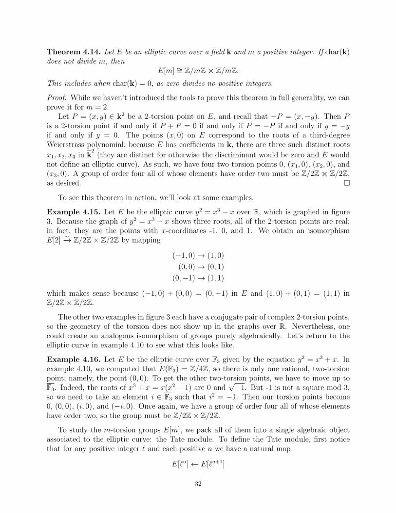
Example 4.15. Let E be the elliptic curve y2 = x3 − x over R, which is graphed in figure3. Because the graph of y2 = x3 − x shows three roots, all of the 2-torsion points are real;in fact, they are the points with x-coordinates -1, 0, and 1. We obtain an isomorphismE[2]

∼−→ Z/2Z× Z/2Z by mapping

(−1, 0) 7→ (1, 0)

(0, 0) 7→ (0, 1)

(0,−1) 7→ (1, 1)

which makes sense because (−1, 0) + (0, 0) = (0,−1) in E and (1, 0) + (0, 1) = (1, 1) inZ/2Z× Z/2Z.

The other two examples in figure 3 each have a conjugate pair of complex 2-torsion points,so the geometry of the torsion does not show up in the graphs over R. Nevertheless, onecould create an analogous isomorphism of groups purely algebraically. Let’s return to theelliptic curve in example 4.10 to see what this looks like.

Example 4.16. Let E be the elliptic curve over F3 given by the equation y2 = x3 + x. Inexample 4.10, we computed that E(F3) = Z/4Z, so there is only one rational, two-torsionpoint; namely, the point (0, 0). To get the other two-torsion points, we have to move up toF3. Indeed, the roots of x3 + x = x(x2 + 1) are 0 and

√−1. But -1 is not a square mod 3,

so we need to take an element i ∈ F3 such that i2 = −1. Then our torsion points become0, (0, 0), (i, 0), and (−i, 0). Once again, we have a group of order four all of whose elementshave order two, so the group must be Z/2Z× Z/2Z.

To study the m-torsion groups E[m], we pack all of them into a single algebraic objectassociated to the elliptic curve: the Tate module. To define the Tate module, first noticethat for any positive integer ` and each positive n we have a natural map

E[`n]← E[`n+1]

32

given by multiplication by `. This looks reminiscent of example 1.11 in which we constructedthe `-adic integers; indeed, the `n-torsion groups form an inverse system

E[`]← E[`2]← E[`3]← · · · ← E[`n]← E[`n+1]← · · ·

with maps given by multiplication by some power of `. The inverse limit of this system isthe object we want.

Definition 4.17. We define the Tate module of an elliptic curve E by Ta`(E) := lim←−nE[`n].

Momentarily, we will use the Tate module to define representations in section 5. Butwhile we’re on the topic of elliptic curves, we define the essential notion of reduction.

4.4 Reduction of Elliptic Curves over Q

Figure 3 depicts the affine piece of the elliptic curve E : y2 = x3 − x over R; by consideringonly the rational points, we may equally well regard E as an elliptic curve over Q. In bothcases, the discriminant is −64 6= 0 so the Weierstrass equation indeed defines an ellipticcurve over either field. In examples 4.10 and 4.16, we went even farther and regarded Eover F3, where this again yields an elliptic curve because −64 6≡ 0 mod 3. This process,of taking an elliptic curve E over Q and instead regarding it as a curve over a finite fieldFp, is called reduction. A question of well-defined-ness arises, however, because of theorem4.8: distinct Weierstrass equations might define the same elliptic curve. And those distinctWeierstrass equations could yield different behaviours mod the same prime p. So we muststandardise our choice.

Definition 4.18. Let E be an elliptic curve over Q. A minimal Weierstrass equationof E is a Weierstrass equation with rational coefficients whose discriminant has the fewestnumber of prime divisors (counted with multiplicity).

Remark 4.19. This definition of minimality relies on the fact that OQ = Z is a principalideal domain (and in fact permits unique factorisation) so we can simultaneously minimizethe number of all prime divisors. For a general number field, OK may not be a P.I.D. inwhich case minimality is better regarded as a local condition for various primes. For K = Q,this amounts to considering elliptic curves over Qp for primes p, but is not necessary for ourdiscussion (which is why we ignore the local perspective; see [Sil86] for elliptic curves over ageneral “local field”).

By the Well-Ordering Principle, minimal Weierstrass equations necessarily exist. Butthey are not unique: the equations y2 = x3 − x and y2 = (x + 1)3 − (x + 1) define thesame (up to isomorphism) elliptic curve E, both have discriminant −64 = 26, and no otherWeierstrass equation representing E has five or fewer total prime divisors. For details onthe existence and construction of minimal Weierstrass equations, see sections 3.1 and 7.1in [Sil86]. From here on out, we represent all elliptic curves over Q with their minimalWeierstrass equations, even when not specifically stated.

Definition 4.20. Let E be an elliptic curve over Q and let E denote the curve obtained byreducing its (minimal) Weierstrass equation mod p. Then two possibilities arise:

33

(i) if p does not divide the discriminant of E, then E is an elliptic curve over Fp; or

(ii) if p divides the discriminant of E, then E has a singularity as a curve over Fp.

In the first case, we say that E has good reduction at p. In the second case, we say thatE has bad reduction at p.

Case (ii) — the case of bad reduction — in fact has two sub-cases, as a Weierstrassequation can have one of two distinct types of singularities: a cusp or a node. The terminol-ogy comes from the geometry of such singularities over R, as depicted in figure 5. Just asthe discriminant ∆ detected when an elliptic curve has a singularity, another invariant willdetect the type of singularity.

Figure 5: The two types of of non-smooth cubic curves. Image adapted from [Sil86].

Theorem 4.21. Let C be a projective curve in P2(k) given by a homogeneous Weierstrassequation. Then

• the curve C is nonsingular if and only if ∆ 6= 0, in which case C is an elliptic curve;

• the curve C has a node if and only if ∆ = 0 and c4 6= 0; and

• the curve C has a cusp if and only if ∆ = 0 = c4.

In addition, C has at most one singularity.

So in reducing a curve over Q mod some prime p, we could end up with three verydifferent types of behaviour. The curve y2 = x3 in figure 5, for example, has a cusp overany finite field (as both its discriminant and c4-value are always 0). In contrast, the curvey2 = x3 +x2 has a cusp only over F2 and has a node over any other finite field. The followingdefinition enumerates the types of reduction.

Definition 4.22. Let E be an elliptic curve over Q and let E denote the reduction of Emod some prime p. We say that

• E has good reduction at p if E defines an elliptic curve over Fp;

34

• E has semi-stable (multiplicative) bad reduction at p if E has a node over Fp;and

• E has unstable (additive) bad reduction at p if E has a cusp over Fp.

The use of the term “stable” refers to the potentially-different behaviour of a curveE/Q when regarded as a curve some over finite extensions of Q. And the use of the terms“additive” and “multiplicative” refer to the structure of the group of points E(Fp) in thosecases. For details, see [Sil86] section 7.4 (noting that there they consider elliptic curves overQp ⊃ Q) and [DS05] section 8.3. Finally, we collect the local behaviour of reductions atvarious primes into a global invariant associated with an elliptic curve over Q.

Definition 4.23. Let E be an elliptic curve over Q and set

ep :=

0, if E has good reduction at p

1, if E has semi-stable reduction at p

2 + δp, if E has unstable reduction at p

where δp is a “small” (≤ 6) correction term which is zero for all p 6∈ {2, 3} (for a moredetailed discussion of δp, see [Sil94]). Define the conductor N of E by

N :=∏

p prime

pep .

Ultimately, the conductor will appear as a level of a newform in the Shimura-TaniyamaConjecture, hence the use of the symbol N . Note that for a semi-stable elliptic curve, theconductor of N is square-free; this case is of interest as Wiles first proved the Shimura-Taniyama Conjecture for semi-stable curves.

5 Galois Representations

In this section, we construct the “Galois representations” associated to an elliptic curve,before then doing the same for a newform.

5.1 Frobenius Elements and Galois Representations

We begin by highlighting some essential structural properties of GQ to facilitate our studyof Galois representations. First, we remark that the action of GQ on Q restricts to an actionon Z ⊂ Q. Indeed, for σ ∈ GQ and x ∈ Z, there exist ai ∈ Z such that

xn + an−1xn−1 + · · ·+ a1x+ a0 = 0

soσ(x)n + an−1σ(x)n−1 + · · ·+ a1σ(x) + a0 = 0

from which it follows that σ(x) ∈ Z. We’ll use the action of GQ on Z to define some importantsubgroups. Fix p ∈ Z prime and let p ⊂ Z be a prime ideal lying over p. The decompositiongroup of p is

Dp = {σ ∈ GQ : σ(p) = p}

35

a subgroup of the absolute Galois group. Because elements of the decomposition group fixp, they induce a natural action on Fp = Z/p: for σ ∈ Dp and x ∈ Z,

σ(x+ p) := σ(x) + p.

At the level of Z, we have (Z∩Z)/(p∩Z) = Z/(p) = Fp; because σ fixes p∩Z, it follows thatthe induced action of σ on Fp fixes Fp. Altogether, in modding everything by p we obtain anatural map Dp → GFp , where GFp = Gal(Fp/Fp).

Theorem 5.1. The reduction map Dp → GFp is a surjection.

Proof. We have seen that the absolute Galois group GQ may be realised as an inverse limitof finite Galois groups Gal(K/Q). In the same way, we can realise GFp as an inverse limitof finite Galois groups Gal(Fq/Fp). We will prove the theorem first in the case of finiteextensions and then pass to the inverse limit to obtain the desired result. To this end, fixa number field K/Q, regard p as an ideal in OK by considering P := p ∩ OK , and regardDp as the decomposition group in Gal(K/Q) by considering D := Dp|K < Gal(K/Q). Forour final piece of setup, denote by Fp the finite field OK/p so that we have a reduction mapD → Gal(Fp/Fp).

Let a ∈ Fp be such that Fp = Fp(a). Consider the polynomial

t(x) =∏σ∈D

(x− σ(a)),

which has a as a root and has coefficients which are fixed by elements of D i.e. t(x) ∈ KD.Then the reduction t(x) mod P — obtained by reducing the coefficients of t(x) mod P —has a as a root and we assert without proof that it is the minimal polynomial of a over Fp.By Galois theory, every Galois conjugate of a is a root of the minimal polynomial of a; thatt(x) is the minimal polynomial thus implies that every Galois conjugate of a takes the formσ(a) for some σ ∈ D. Because a generates the extension Fp/Fp, it follows that every elementof Gal(Fp/Fp) appears as some σ so the reduction map D → Gal(Fp/Fp) surjects.

Now, return to the infinite extensions and take an automorphism σ ∈ GFp . Regard GFp

as an inverse limit of finite Galois groups so that we may represent σ with a compatiblesystem (σn)n∈I of elements σn ∈ Gal(Fpn/Fp), where pn := p ∩ Kn for some number fieldKn and Fpn = Fpn = OKn/pn. For each pn our work in the finite case shows we can finda σn ∈ Dp|Kn such that the reduction of σn is precisely σn. These σn necessarily form acompatible system for the groups Gal(Kn/Q), because they arose from a compatible system(σn)n∈I . Then the inverse limit knits together the (σn)n∈I into an element σ ∈ GQ whichreduces to σ. And so the reduction map Dp → GFp surjects.

We now define the inertia group of p to be the kernel of the reduction map Dp → GFp ,

Ip = {σ ∈ Dp : σ(x) ≡ x mod p for all x ∈ Z},

so that we have a short exact sequence

0→ Ip → Dp → GFp → 0.

36

As a field of characteristic p, there is a natural automorphism of Fp: the Frobeniusautomorphism φp defined by φp(x) := xp. We define a Frobenius element Frobp to be anyelement of the decomposition group which maps to φp ∈ GFp . Equivalently, a Frobenius

element Frobp is any element of GQ such that for all x ∈ Z,

Frobp(x) ≡ φp(x) = xp mod p.

Note that, by the short exact sequence above, the Frobenius element Frobp always exists butis only defined up to multiplication by the kernel Ip.

Ideally, we would like to have a notion of Frobp in which our Frobenius element dependsonly the prime p and not on our choice of p lying over p. While we cannot quite obtain such aunique Frobenius element in general, we can speak of a Frobenius element up to conjugation.

Theorem 5.2. Let p and p′ be primes lying over p. Then there exists σ ∈ GQ such thatσ(p) = p′ and

σFrobpσ−1 = Frobσ(p) = Frobp′ .

In particular, any two primes p and p′ lying over p have conjugate Frobenius elements.

Proof. We won’t prove the existence of such a σ ∈ GQ as it isn’t our main focus. So assumeσ(p) = p′. Then the definition of Frobp yields

Frobp is a Frobenius over p ⇐⇒ Frobp(σ−1x) ≡ (σ−1x)p mod p

⇐⇒ Frobp(σ−1x)− (σ−1x)p ∈ p

⇐⇒ σFrobpσ−1x− xp ∈ σ(p)

⇐⇒ σFrobpσ−1x ≡ xp mod σ(p)

⇐⇒ σFrobpσ−1 is a Frobenius over σ(p)

⇐⇒ σFrobpσ−1 = Frobσ(p)

as desired.

Of course, a natural concern arises: when we write σFrobpσ−1 = Frobσ(p), the left-hand-side

is only defined up to Ip while the right-hand-side is only defined up to Iσ(p). We allow thisambiguity because once again we have equality up to conjugation:

Dσ(p) = σDpσ−1 and Iσ(p) = σDpσ

−1.

Now, we care so much about Frobenius elements because they form a dense subset of“much” of the absolute Galois group. Indeed, although we would like a dense subset of allof GQ, we have to settle for something a touch weaker.

Theorem 5.3 (A Simple Version of the Chebotarev Density Theorem). Let S be a finiteset of primes in Z and let Qunr,S denote the maximal extension of Q unramified outside ofS i.e. the union of all finite extensions L/Q for which any prime p 6∈ S does not ramify inOL. For each prime p 6∈ S, let

Fp =⋃p|p

{conjugacy class of Frobenius elements Frobp|Qunr,S}.

Then the union of all such Fp is dense in Gal(Qunr,S/Q). Succinctly, the Frobenius elementsof unramified primes are dense in Gal(Qunr,S/Q).

37

In this statement, density is determined with respect to the Krull topology.That we have a dense set is of great interest for continuity reasons: the image of a con-

tinuous map on Gal(Qunr,S/Q) is completely determined by the map’s image on Frobeniuselements Frobp. As we have seen, however, the symbol Frobp is only defined up to con-jugation, so it makes sense to study continuous maps which are themselves defined up toconjugation; this motivates our study of representations in the next section which are, bydefinition, determined only up to conjugation.

Definition 5.4. A d-dimensional `-adic Galois representation is a continuous homo-morphism

ρ : GQ → GLd(L)

where L is a finite extension of Q`. Continuity is determined with respect to the Krulltopology on the domain and the subspace toplogy (of Ld2) on the codomain. Two Galoisrepresentations ρ1, ρ2 are isomorphic if there exists a matrix M ∈ GLd(L) such that ρ1(g) =Mρ2(g)M−1 for all g ∈ GQ.

The Galois representations associated to elliptic curves will have L = Q` while the Galoisrepresentations associated to a newform f will have L = Kf,λ, a finite extension of Q`

obtained from the number field Kf .Just as we had a notion of ramification for primes in a number field, so too does there

exist a notion of ramification for Galois representations. In both cases, ramification dependson the behaviour for a prime p lying above a rational prime p.

Definition 5.5. Let ρ : GQ → GLd(L) be a Galois representation. We say that ρ isunramified at a prime p ∈ Z if for any prime p ⊂ Z lying over p, the inertia group is killedby ρ i.e. Ip ⊂ ker ρ.

So we now have two uses of the word “unramified”: a number field in which p is unramifiedand a Galois representation which is unramified at p. Let’s connect these two ideas. Notethat ρ necessarily factors through a unique quotient as in the commutative diagram

GQ GL2(Q`)

Gal(Qker ρ/Q)

r

ρ

i

such that i is injective, where Qker ρdenotes the fixed field of ker ρ and r denotes the natural

restriction map. If ρ is unramified at p, then for all p lying above p, we have ker ρ ⊃ Ip. It

turns out that this implies that p will be unramified in Qker ρ, so ρ in some sense kills the

part of GQ where p ramifies. We care about ramification because of theorem 5.3, for whichwe need to exclude finitely-many ramified primes.

5.2 Galois Representation Associated to an Elliptic Curve

Let E be an elliptic curve over Q. To define a Galois representation associated to E, weconsider the natural action of GQ on E. In particular, an automorphism σ ∈ GQ acts on a

38

point [x1 : x2 : x3] of E, xi ∈ Q, by acting componentwise: σ([x1 : x2 : x3]) := [σ(x1) : σ(x2) :σ(x3)]. Note that the action produces a well-defined map on P3(Q) because homomorphismsare multiplicative.

Now, recall that multiplication by m on E may be written as rational polynomials withrational coefficients; because the coefficients are fixed by σ ∈ GQ, the action of the absoluteGalois group commutes with multiplication by m. That is, GQ sends torsion subgroups intothemselves, so the action restricts to E[`n] for all positive ` and n. Regard the action of GQon `n-torsion as a map σn : GQ → Aut(Z/`nZ) to obtain the following commutative diagram

GQ

Aut(E[`n]) Aut(E[`n+1]),

σn σn+1

where the bottom map Aut(E[`n+1]) → Aut(E[`n]) arises from the natural multiplication-by-` map E[`n+1]→ E[`n]. But by theorem 4.14, we have an isomorphism E[`n] ∼= (Z/`nZ)2.Thus, Aut(E[`n]) ∼= GL2(Z/`nZ) and the diagram becomes

GQ

Aut(E[`n]) Aut(E[`n+1])

GL2(Z/`nZ) GL2(Z/`n+1Z))

σn σn+1

o o

Applying the inverse limit — remembering that lim←−nE[`n] = Ta`(E) and lim←−n Z/`nZ = Z`

— we obtain a series of maps

GQ → Aut(Ta`(E))∼−→ GL2(Z`) ↪→ GL2(Q`).

Their composition yields a map ρE,` : GQ → GL2(Q`).

Definition 5.6. The map ρE,` : GQ → GL2(Q`) obtained in the preceding construction isthe `-adic Galois representation associated to the elliptic curve E. Note that dependence onE enters in the action of GQ on the Tate module Ta`(E).

Recall that for ρE,` : GQ → GL2(Q`) to define a Galois representation, it must becontinuous. We’ll argue continuity assuming theorem 1.14 and the following fact: a basis forthe topology on GL2(Q`) is the collection

{UM(n)}M∈GL2(Q`),n∈Z≥0, where UM(n) := M(I + `nM2(Z`))

and Md(Z`) denotes the set of d by d matrices with entries in Z`. Because a map is continuousif and only if the inverse image of any basis set is open, we need only show that ρ−1E,`(Um(n))is open for all M and n. Moreover, multiplication by M ∈ GL2(Q`) defines a continuousmap on GL2(Q`), so it actually suffices to show that ρ−1E,`(U1(n)) is open for all m.

39

Take M ∈ U1(n) and note that for any e ≤ n we have M ≡ I mod `e. In particular,

M = (I, . . . , I︸ ︷︷ ︸n times

,Mn+1,Mn+2, . . .) (7)

where Me denotes the reduction of M mod `e. As such, when we pull M back along ρ−1E,` toGQ, we wind up with elements of the form

(1, . . . , 1︸ ︷︷ ︸n times

, σin+1 , σin+2 , . . .) ∈ GQ (8)

where the first n identity entries correspond to finite Galois extensions Gal(Kij/Q) contain-ing the `j-torsion coordinates. Moreover, every element in GQ of the form in (8) maps tosomething of the form in (7). So we have

H := ρ−1E,`(Um(n)) = {σ ∈ GQ : σ = (1, . . . , 1︸ ︷︷ ︸n times

, σin+1 , σin+2 , . . .)},

a subgroup of GQ whose elements fix the number fields Kij . But then QH=⋃nj=1Kij is a

finite extension of Q such that H = Gal(KH/Q). In particular, theorem 1.14 says that H isopen in the Krull topology, so ρE,` is continuous.

Now that we have the Galois representation ρE,`, we enumerate some of its properties.

Theorem 5.7. Let E be an elliptic curve over Q with conductor N and fix a prime `. ThenρE,` is unramified for all primes p - `N and for any p a prime lying over p, the imageρE,`(Frobp) satisfies the equation

x2 − ap(E)x+ p = 0,

where ap(E) := p+ 1−#E(Fp). Moreover, ρE,` is irreducible.

For clarification, we use # to denote cardinality. There are four important things to remark.First, note that the characterstic polynomial of ρE,`(Frobp) is entirely independent of `,

and instead only depends on E and p.Second, that ρE,` is unramified at all but the finitely many primes dividing `N shows that

ρE,` factors through a Galois group simpler than all of GQ. To see this, let S denote the set ofprimes dividing `N and denote by H the smallest closed normal subgroup of GQ containingIp for all p 6∈ S — we require that H be normal to avoid the ambiguity of conjugate inertialgroups. By virtue of being unramified outside of S, the representation ρE,` is trivial on H.Apply the fundamental theorem of infinite Galois theory — which gives a correspondencebetween intermediate fields and closed subgroups of the Galois group (see [Mil18]) — to see

that H = Gal(Q/QH) and QH

is Galois over Q. The following lemma identifies QHmore

explicity.

Lemma 5.8. We have QH= Qunr,S, the maximal extension of Q unramified outside of S.

By the lemma, H = Gal(Q/Qunr,S). Because ρE,` kills the generators of H, the continuityof ρE,` and that H is closed imply that ρE,` kills all of H = Gal(Q/Qunr,S). So ρE,` is entirelydetermined by its action at the level of Qunr,S/Q, rather than Q/Q. And so we have provenour desired result.

40

Theorem 5.9. The representation ρE,` : GQ → GL2(Q`) factors through Gal(Qunr,S/Q).That is, we have a commutative diagram

GQ GL2(Q`)

Gal(Qunr,S/Q)

r

ρE,`

ρ

where r denotes the natural restriction map and ρ is the unique continuous map which fillsin the diagram.

Third, because the Frobenius element Frobp is only determined up to conjugation, acharacteristic equation x2− ap(E)x+ p = 0 is the best possible determination of ρE,`(Frobp)we could hope for. Two conjugate Frobenius elements might have distinct images in GL2(Q`),but as conjugates they will necessarily have the same characteristic equation.

Fourth, the two previous remarks allow us to appeal to the Chebotarev density theorem(theorem 5.3). Indeed, the density of the Frobenius elements (of unramified primes) inGal(Qunr,S/Q) tells us that ρ is entirely determined by where it sends Frobenii. So thecommutative diagram shows that ρE,` is itself determined by its image on (unramified)Frobenii. But theorem 5.7 provides the characteristic equations of these Frobenius elements,so checking the equality of ρE,` and some other representations reduces to checking equalityonly at Frobenius elements. We will return to these idea in section 6, after constructingsimilar representations for newforms.

5.3 Galois Representation Associated to a Newform

Let f ∈ M2(Γ1(N)) be a newform and let X1(N) denote H ∪ Q ∪ {∞} mod the action ofΓ1(N) as in definition 2.12. Note that f has weight k = 2; as weight two newforms are theonly ones to appear in the STC correspondence, we need only consider Galois representationsfor weight-2 forms.

The construction of the Galois representation associated to f is much more complicatedthan that for an elliptic curve, and we simply have not developed the necessary backgroundhere. As such, we offer only an outline and refer the reader to section 9.5 of [DS05] foradditional details. The construction proceeds in three stages:

1. Regard X1(N) as a curve over C and then transfer this to X1(N) as a curve over Q(by analyzing the fields of meromorphic functions on each). Then the first step is toconstruct a Galois representation

ρX1(N),` : GQ → GL2g(Q`)

where g is the “genus” of X1(N) as a curve over Q.

2. Associate to f a “complex torus” Af with dimension d. Then construct a Galoisrepresentation

ρAf ,` : GQ → GL2d(Q`)

where we use the representation ρX1(N),` in part 1 to prove that ρAf ,` is indeed arepresentation with some nice properties.

41

3. Decompose the representation ρAf ,` into some natural pieces to obtain representations

ρf,λ : GQ → GL2(Q`)

where λ is any prime lying over ` in the number field Kf .

In steps 1 and 2, the construction of ρX1(N),` and ρAf ,` proceeds quite similarly to that ofρE,` for E an elliptic curve. Indeed, one can define the Tate module of both (the “Jacobian”of) X1(N) and Af using `n-torsion and then construct the representation as before. In thiscase, however, the points on either X1(N) or Af don’t necessarily form a group (in this way,elliptic curves are quite special), so one needs to use the “Picard group” of the curve/surface;for an elliptic curve E, the Picard group of E is isomorphic to the group of points on E sothis more general construction agrees with what we did for elliptic curves. Either way, theTate modules Ta(X1(N)) and Ta(Af ) arise as inverse limits of torsion as before. Similar tothe elliptic curve case, this process yields isomorphisms Ta(X1(N)) ∼= Z2g

` and Ta(Af ) ∼= Z2d`

and so obtain representations with dimensions 2g and 2d.The isomorphism Ta(Af ) ∼= Z2d

` becomes quite important for step 3 as well. TensoringZ2d` with Q` over Z` in effect inverts the elements of Z` so that

V`(Af ) := Ta(Af )⊗Z`Q`∼= Q2d

`

is the vector space underying the representation ρAf ,`. Thus, to decompose ρAf ,` we needonly decompose V`(Af ).

Lemma 5.10. We have a decomposition V`(Af ) ∼= (Kf ⊗Q Q`)2.

So it remains to decompose Kf ⊗Q Q`. We will do this for an arbitrary number field beforethen specializing to the case of Kf .

Let K be a number field with ring of integers OK and fix a prime `. For each ideal λlying over `, define the ring of λ-adic integers OK,λ by the inverse limit

OK,λ = lim←−n

OK/λn

and define the field of λ-adic numbers Kλ as the field of fractions of OK,λ. Notice thatthis agrees with the definition of the `-adic integers/numbers in example 1.11 by takingK = Q. Indeed, because `Z ⊂ λOK, there is a natural embedding of Z` ↪→ OK,λ and thus anembedding Q` ↪→ Kλ. The latter makes Kλ into a field extension of Q`, and the extension isfinite because K/Q is. Now, we can state our desired result and apply it to our particularcase.

Lemma 5.11. We have a decomposition K⊗QQ`∼=∏

λ|`Kλ where the notation λ|` denotesthat the product ranges over all primes λ ⊂ OK lying over `.

Proof. Refer to section 9.2 of [DS05] the proof.

For λ a prime in Kf lying over `, denote by Kf,λ the field of λ-adic integers. Togetherthe lemmas say that

V`(Af ) ∼=

∏λ|`

Kf,λ

2

42

so that the representation ρAf ,λ yields a homomorphism

GQ → GL2

∏λ|`

Kf,λ

.

For a fixed λ, we may apply a projection from the product to obtain a homomorphism

ρf,λ : GQ → GL2 (Kf,λ) .

Definition 5.12. The homomorphism ρf,λ is the `-adic Galois representation associated tothe newform f .

Contrast the two representations we have constructed: the Galois representation ρE,`appeals to the case of definition 5.4 when L = Q`, whereas ρf,λ requires a finite extensionL = Kf,λ. For these definitions to align — as they must for our desired correspondence —we will need Kf,λ = Q`. Based on the definition of Kf,λ, this occurs when Kf = Q. Aswe will see in the next section, the Shimura-Taniyama Conjecture provides the existenceof such newforms. But first we again summarise the properties of the representation justconstructed; note their incredible similarity to those of ρE,`.

Theorem 5.13. Let f ∈ S2(N,χ) be a newform with number field Kf and fix a prime `. Foreach prime λ of OKf

lying over `, let ρf,λ : GQ → GL2(Kf,λ) be the Galois representationassociated to f . Then ρf,λ is unramified at primes away from ` and N (i.e. is unramifiedfor every prime p - `N). Moreover, for p a prime over p, ρf,λ(Frobp) satisfies the equation

x2 − ap(f)x+ χ(p)p = 0.

In particular, if f ∈ S2(Γ0(N)) then χ(p) = 1 so that the equation becomes x2−ap(f)x+p = 0.

Note once again that the characteristic equation of ρf,λ(Frobp) does not depend on `!Indeed, for the representations ρf,λ and ρE,` to align, we’ll want their characteristic equationsat Frobp to agree. As in the theorem, this case occurs when f ∈ S2(Γ0(N)). The Shimura-Taniyama Conjecture will guarantee that such newforms suffice to give a correspondence, solet’s finally get on to stating STC.

6 The Shimura-Taniyama Conjecture

In its many forms, the Shimura-Taniyama Conjecture (STC) states that every elliptic curveis “modular”. In this paper we have developed theory for understanding the Galois theoreticstatement of STC, the version which Wiles proved (with some help from Taylor) in 1995:

Theorem 6.1. (Galois Theoretic STC for Semi-Stable Elliptic Curves) Let E be a semi-stable elliptic curve over Q with conductor N . Then there exists a newform f ∈ S2(Γ0(N))with number field Kf = Q such that ρf,` ∼ ρE,` for all `.

43

Thus, a semi-stable elliptic curve E/Q is called “modular” because it corresponds —through its Galois representations — to some modular form f . We of course have no hope ofgoing through the proof of STC here. Instead, we go through an example which illustratesthe incredible power of this correspondence.

Consider the congruence subgroup Γ0(11) and let X0(11) denote Γ0(11)\H∗ as in defi-nition 2.12. The expository article [Wes99] goes through and deduces that a fundamentaldomain for X0(11) is the blue region in figure 6. Note that, although the fundamental do-main has five limits on the real line, X0(11) only has two distinct cusps. Indeed, figure 7shows the fundamental domain wrapped up with two sides identified; the two cusps are thecusp at infinity in the center of the square and the single cusp at all four vertices of thesquare. From topology, we recognise the square with these side identifications as a torus, sowe can realise X0(11) as a compact surface with genus one.

Figure 6: A fundamental domain for Γ0(11). The arrows denote sides which are identifiedunder the action of some matrix of Γ0(11). Notice that this fundamental domain neverthelesscontains a fundamental domain for SL2(Z), but contains one different from that in figure 1.Image adapted from [Wes99].

Figure 7: The fundamental domain for Γ0(11) in figure 6 with the triple-arrow boundariesidentified and the other boundaries straightened. Image adapted from [Wes99].

Alternatively, an algebraic argument in section 3.1 and exercise 3.1.4 of [DS05] deduces

44

that the genus of X0(11) is b11+112c = 1. Either way, recalling that an elliptic curve is a

smooth projective curve of genus 1 allows us to regard X0(11) itself as an elliptic curve! (Weignore the subtle connections between the genus of a surface and the genus of a curve here;[Wes99] explicitly goes through the process of transferring X0(11) from a genus one surfaceto a genus one curve over Q.)

Because X0(11) defines an elliptic curve, it has an associated Weierstrass equation (6).Once again, refer to [Wes99] for the details of how to discern that X0(11) has (minimal)Weierstrass equation

E : y2 + y = x3 − x2 − 10x− 20

as an elliptic curve E over Q. Equation in hand, let’s see what the Shimura-TaniyamaConjecture, theorem 5.7, and theorem 5.13 say about E and its corresponding newform f .

By STC, we can determine the level N of f by determining the conductor of E. Recallingthe notation from definition 4.7, we have that

b2 = −4,

b4 = −20,

b6 = −79, and

b8 = −21.

so that E has discriminant∆ = −161, 051 = −1 · 115

and c4 valuec4 = 496 = 24 · 31.

The discriminant shows that E has bad reduction at 11 and good reduction at all otherprimes. Because 11 does not divide the c4 value, E has semi-stable (multiplicative) reductionat 11 so definition 4.23 yields that that E has conductor N := 11. So by STC we seek anewform f ∈ S2(11).

Comparing theorems 5.7 and 5.13 and the images of our Galois representations at Frobe-nius elements, we see that ρE,` ∼ ρf,` forces

x2 − ap(E)x+ p = x2 − ap(f)x+ p

for all p - 11 · `. Varying `, we obtain p + 1 −#E(Fp) = ap(E) = ap(f) for all p 6= 11. Wethus compute a couple values of #E(Fp) to get the first couple Fourier coefficients of f .

• For p = 2, we have an equation E : y2 + y = x3 +x2. By Fermat’s Little Theorem modtwo, this reduces to y+ y = x+x which holds for all points (x, y) ∈ F2

2. Together withthe point at infinity, we have #E(F2) = 5 so that a2(E) = 2 + 1− 5 = −2.

• For p = 3, reduction yields E : y2 +y = 2x2 +1 (again using Fermat’s Little Theorem).If y = 0, then x = ±1 and if x = 0, there are no solutions with y ∈ F3. So if neitherx nor y equals zero, we may use a2 = 1 mod 3 for a 6= 0 to obtain y + 1 = 0. Thisgives the points y = −1 and x = ±1. Together with the point at infinity, we count#E(F3) = 5 so that a3(E) = 3 + 1− 5 = −1.

45

• For p = 5, similar arguments become increasingly casewise (but no less interesting oruseful); for brevity, we had a computer check all twenty-five to discover that four pointslie on E: (0, 0), (0, 4), (1, 0), and (1, 4). So #E(F5) = 5 so that a5(E) = 5 + 1− 5 = 1.

It follows by STC that

f(q) = q − 2q2 − q3 + a4(f)q4 + q5 + · · ·and, if we had further knowledge of the Dirichlet character χ for which f ∈ S2(11, χ), wecould determine a4(f) using a2(f). The prime coefficients suffice, however, in the followingway.

Chapter 3 of [DS05] computes dimension formulas for the vector spaces (over C) of mod-ular forms Mk(Γ0(N)) and of cusp forms Sk(Γ0(N)). In particular, the dimension is alwaysfinite and (as we’ve seen previously in theorem 3.22) the set of newforms constitutes a basisfor the subspace Sk(Γ0(N))new ⊂ Sk(Γ0(N)). So in computing enough Fourier coefficientsap(f), we can uniquely determine which of the finitely-many newforms f must be. Referenc-ing the dimension formulas in [DS05], we find that dimC S2(Γ0(N)) is the genus of X0(N)as a Riemann surface. For N = 11, in particular, we have that the dimension of S2(Γ0(11))equals 1 so there is but one possible newform: the unique newform of weight 2 and level 11,label 11.2.a.a in the LMFDB:

f(q) = q − 2q2 − q3 + 2q4 + q5 + 2q6 − 2q7 − 2q9 − 2q10 + q11 − 2q12 + 4q13 + · · · .As they must, the Fourier coefficients we have so far computed agree with those given

on LMFDB. Indeed, that a7(f) = −2 in turn implies that E(F7) has 10 points and thata13(f) = 4 implies that E(F13) has 10 as well. Notice that we do not obtain information forp = 11 because the correspondence ap(f) = ap(E) only holds for primes of good reduction(i.e. for primes not dividing the conductor N). Theorem 5.9 and the discussion whichfollows justify that the equality of images of Frobenius elements at good primes ensuresthe correspondence ρE,` and ρf,` of the Galois representations at all primes `. At the badprimes ` dividing N , the behaviour of the Galois representations are more complicated —notice that theorems 5.7 and 5.13 only give information for good primes — but one cannevertheless make sense of the correspondence there. For details on the correspondence atprimes of semi-stable and unstable reduction, refer to chapters 4 and 5 of [Sil94].

Let’s compute one more example, so that that we can see a case when S2(Γ0(N)) hasdimension greater than one. In particular, consider the elliptic curve E with (minimal)Weierstrass equation y2 + y = x3 + x − 1. In the same manner as before we can computethat E has discriminant ∆ = −1 · 307 and c4 value c4 = −48. Thus, E has semi-stable badreduction at 307 and no other primes, and thus has conductor N = 307. So STC guaranteesthat E corresponds to some newform f ∈ Sk(Γ0(307)).

As before, we appeal to chapter 3 of [DS05] for the dimensions of the spaces of cuspforms; exercise 3.1.4 and section 3.5 together show that dimC S2(Γ0(307)) = 25. BecauseN = 307 is prime, S2(Γ0(307)) = S2(Γ0(307))new and this means that there are twenty-fivenewforms of weight 2 and level 307. Of these, only four have number field Q:

f1(q) := q −2q4 +4q5 −3q9 + · · ·f2(q) := q +2q2 +2q3 +2q4 +4q6 −3q7 +q9 + · · ·f3(q) := q +2q2 +2q4 +2q5 +3q7 −3q9 + · · ·f4(q) := q +q2 +2q3 −q4 +2q6 +3q7 −3q8 +q9 + · · · .

46

So STC requires that one of the four newforms fi corresponds to E. Compute that #E(F2) =1 to narrow the choices to f2 and f3. Then compute that #E(F3) = 4 to determine thatE has corresponding newform f3. It follows that #E(F7) = 5 and — using LMFDB to seethat a97(f3) = 11 — that #E(F97) = 87.

7 Overview of the Proof of Fermat’s Last Theorem

Historically, the proof of Fermat’s Last Theorem (FLT) proceeded through a series of re-ductions. In 1995, Wiles (with some help from Taylor) added the final link in the chain byproving the Shimura-Taniyama Conjecture (STC) for semi-stable elliptic curves. The proofmanifests as an enormous proof by contradiction, as it begins by assuming a hypotheticalsolution to a` + b` = c` with abc 6= 0 and ` > 7 and ultimately contradicts the non-existenceof modular forms of weight k = 2 and level N = 2:

1. In 1955, Shimura and Taniyama make their famous conjecture that all elliptic curvesover Q (in particular, the semi-stable ones) are modular.

2. In 1975, Hellegouarch took a hypothetical non-trivial solution a`+b` = c` to the Fermatequation and considered the elliptic curve

E : y2 = x(x+ a`)(x− b`).

Subsequent work by Frey showed that E is semi-stable and that its associated Galoisrepresentation ρE,` is irreducible for ` > 7. By passing through STC, this linked FLTwith modular forms.

3. In the late 80’s, Serre devised an incredible series of powerful conjectures, which detailhow various Galois representations “arise” from modular forms in a precise way. Inparticular, Serre conjectured that the Galois representations ρE,` associated to theFrey-Hellegouarch curve arise from modular forms of weight k = 2 and level N = 2.

4. In 1990, Ribet proved that the Shimura-Taniyama conjecture implies Serre’s conjecturefor the representations ρE,`. Because there are no modular forms of weight k = 2 andlevel N = 2, the truth of STC would contradict the existence of the elliptic curve E,which in turn contradicts the existence of a solution a` + b` = c`.

5. In 1995, Wiles (with some help from Taylor) furnished the final link in the chain byproving STC for semi-stable elliptic curves with irreducible representations ρE,`; by theproperties of the Frey Curve E, Wiles’s work sufficed to prove Fermat’s Last Theorem.

And so, 358 years after Fermat’s original note, the mathematical community completed theproof of Fermat’s Last Theorem. While we have highlighted many mathematicians here,without a doubt there are hundreds of others who contributed.

We stated the Shimura-Taniyama Conjecture for semi-stable elliptic curves over Q asthis case suffices to prove Fermat’s Last Theorem. But the full conjecture in fact postulatedthat all elliptic curves over Q — not just the semi-stable ones — are modular. By 2001,work of Breuil, Conrad, Diamond, and Taylor had completed the general case so that we

47

now know that all rational elliptic curves are modular; this result is sometimes called theModularity Theorem, rather than the Shimura-Taniyama Conjecture. Even more recently,Robert Langlands has devised a series of conjectures which vastly generalise the ModularityTheorem. The so-called Langlands program thus seeks to correspond “automorphic forms”— natural generalisations of modular forms — to various arithmetic objects in algebraicgeometry — such as elliptic curves. Already these conjectures guide the future of numbertheory, just as Shimura-Taniyama inspired twentieth century number theorists.

48

References

[DDT07] Henri Darmon, Fred Diamond, and Richard Taylor. Fermat’s last theorem, Septem-ber 2007.

[DS05] Fred Diamond and Jerry Shurman. A First Course in Modular Forms. SpringerScience and Business Media, New York, 2005.

[Mil17] James S. Milne. Algebraic number theory, 2017. Available at www.jmilne.org/

math/.

[Mil18] James S. Milne. Fields and galois theory, 2018. Available at www.jmilne.org/

math/.

[Rid09] Larry Riddle. Sophie germain and fermat’s last theorem, July 2009. Available athttps://www.agnesscott.edu/lriddle/women/women.htm.

[Sch18] Berndt Schwerdtfeger. Modular fundamental domain, October 2018.

[Sil86] Joseph H. Silverman. The Arithmetic of Elliptic Curves. Springer Science andBusiness Media, New York, 1986.

[Sil94] Joseph H. Silverman. Advanced Topics in the Arithmetic of Elliptic Curves.Springer Science and Business Media, New York, 1994.

[Wes99] Tom Weston. The modular curves X0(11) and X0(11), 1999. Available at https://people.math.umass.edu/~weston/ep.html.

49