modular road system - university of waterloo
TRANSCRIPT
Modular Road Plate System
by
Tin Lun Alan Mak
A thesis
presented to the University of Waterloo
in fulfillment of the
thesis requirement for the degree of
Master of Applied Science
in
Civil Engineering
Waterloo, Ontario, Canada, 2012
©Tin Lun Alan Mak 2012

ii
AUTHOR'S DECLARATION
I hereby declare that I am the sole author of this thesis. This is a true copy of the thesis, including any
required final revisions, as accepted by my examiners.
I understand that my thesis may be made electronically available to the public.

iii
Abstract
Concrete and asphalt are the most common materials used in permanent roadway pavements. Roadways
are also constructed for temporary use in the resource industry, for remote site construction, and for disaster
relief. Although temporary roads have been used for almost as long as permanent ones, little research has been
done to optimize their design in view of their relatively short service lives or to investigate the advantages of
constructing them with reusable materials or employing structural systems that require minimal subgrade
preparation. With this in mind, the purpose of this study is to conduct research to determine the feasibility of a
reusable, modular road plate system requiring minimal preparation of the subgrade.
This thesis presents a literature review, summarizing the currently available products that perform a similar
function and the methods currently available to design such products, including terramechanics and foundation
design. Alternative concept designs for a modular road plate system are then introduced. Following this, a
simple structural steel plate system is designed to resist vertical, traffic-induced loads using several methods.
Specifically, an equivalent thickness method and finite element (FE) analysis are employed. Different loading
conditions, soil conditions, and plate assemblies (i.e. boundary conditions) are compared. The different loading
conditions include: single and multi-wheel loading, and centre versus edge loading of the plate. The different
modelled plate assemblies include: single plates, four plates assembled with fixed connections, and four plates
assembled with hinged connections. Structural steel plates are considered in the FE analysis study, in order to
develop the design methodology, prior to applying it to the other materials or structural systems. Soil properties
and panel thicknesses are studied covering a broad range of conditions under which temporary roadways may
be built. Thirty scenarios are created from five soil types and six panel thicknesses. With the different loading
and boundary conditions investigated, a total of 120 scenarios are analyzed in total, using several different FE
models.
The results from the FE analysis studies show that there is a significant difference between hinged and fixed
connected panels, and that these different boundary conditions can be considered by modelling a single plate
that is centre loaded (to represent a multi-plate system with fixed plate connections) or a single plate that is edge

iv
loaded (to represent a multi-plate system with hinged plate connections). The results of this research in general
provide a practical framework for developing a modular road plate system constructed using any material or
structural system under a range of soil and loading conditions.

v
Acknowledgements
I would like to thank my supervisors, Dr. Scott Walbridge, P.Eng., Dr. Susan Tighe, P.Eng., and Dr. Alan
Plumtree, P.Eng., for their contribution to this work by providing research advice, academic guidance, and
engineering support. Their knowledge and expertise help aid and guide the completion of this research.
My special thanks to Vale and the Ontario Centres of Excellence (OCE) for their financial support and
patience. In particular, I would like to express my appreciation to Dr. Sam Marcuson (Vale), Ross Bradsen
(OCE), Leanne Gelsthrope (OCE), David Doran (OCE), and James Doran (OCE).
Lastly, I would like to thank my lab mates, Jeff, Kasra, Greg, Rana, David, and Jamie for their continuous
support and motivation.

vi
Dedication
To my lovely wife, faithfully will forever be engraved.

vii
Table of Contents
AUTHOR'S DECLARATION ............................................................................................................... ii
Abstract ................................................................................................................................................. iii
Acknowledgements ................................................................................................................................ v
Dedication ............................................................................................................................................. vi
Table of Contents ................................................................................................................................. vii
List of Figures ........................................................................................................................................ x
List of Tables ........................................................................................................................................ xii
Chapter 1 Introduction ............................................................................................................................ 1
1.1 Background .................................................................................................................................. 1
1.2 Objectives ..................................................................................................................................... 3
1.3 Scope ............................................................................................................................................ 3
1.4 Thesis Organization ...................................................................................................................... 3
Chapter 2 Literature Review .................................................................................................................. 5
2.1 Current Pavement Methods .......................................................................................................... 5
2.1.1 AASHTO Design Guide ........................................................................................................ 5
2.1.2 StreetPave .............................................................................................................................. 7
2.2 Existing Modular Road Systems .................................................................................................. 8
2.2.1 Rollable Systems ................................................................................................................... 8
2.2.2 Plate Systems ......................................................................................................................... 9
2.3 Temporary Road Research ......................................................................................................... 13
2.4 Existing Tools for Designing Modular Road Plate Systems ...................................................... 14
2.4.1 Terramechanics.................................................................................................................... 14
2.4.2 Foundation Designs ............................................................................................................. 17
2.4.3 Finite Element (FE) Analysis .............................................................................................. 21
2.5 Summary of Findings ................................................................................................................. 22
Chapter 3 Design Criteria ..................................................................................................................... 23
3.1 Performance ................................................................................................................................ 23
3.1.1 Structural: Vertical Loads .................................................................................................... 23
3.1.2 Structural: Horizontal Loads ............................................................................................... 27

viii
3.1.3 Skid Resistance ................................................................................................................... 28
3.2 Cost ............................................................................................................................................ 29
3.3 Durability ................................................................................................................................... 31
3.4 Research Methodology for Vertical Load Design ..................................................................... 33
3.5 Material Properties and Limits for Vertical Traffic Load Design .............................................. 34
3.5.1 Road Plate: Material Properties and Strength Limits .......................................................... 34
3.5.2 Soil: Material Properties and Strength Limits ..................................................................... 35
3.5.3 Vertical Deformation Limits ............................................................................................... 38
3.6 Summary of Key Findings ......................................................................................................... 40
Chapter 4 Design Concepts .................................................................................................................. 42
4.1 Material Type ............................................................................................................................. 42
4.1.1 Conventional Pavement Materials (i.e. Asphalt, Concrete) ............................................... 42
4.1.2 Metals .................................................................................................................................. 43
4.1.3 Polymers ............................................................................................................................. 46
4.1.4 Fibre-Reinforced Polymers ................................................................................................. 48
4.1.5 Wood ................................................................................................................................... 48
4.2 Modular Road System Design Concepts ................................................................................... 49
4.2.1 Simple Plate Design ............................................................................................................ 49
4.2.2 Sandwich Panel Design ....................................................................................................... 54
4.2.3 Asphalt Tray Design ........................................................................................................... 54
4.2.4 Railway-Inspired Design ..................................................................................................... 55
4.3 Equivalent Plate Thickness Calculations ................................................................................... 56
4.3.1 Calculation Methodology .................................................................................................... 57
4.3.4 Assumed Input Parameters .................................................................................................. 59
4.3.5 Calculation Results ............................................................................................................. 60
4.3.6 Other Trial Thickness Considerations ................................................................................. 61
4.4 Summary of Key Findings ......................................................................................................... 62
Chapter 5 Finite Element (FE) Model and Study Descriptions ........................................................... 63
5.1 2D Single Wheel (2D-SW) FE Model ....................................................................................... 63
5.2 Multi-Wheel (2D-MW) Model .................................................................................................. 67

ix
5.3 3D Single Wheel (3D-SW) Model ............................................................................................. 68
5.4 Modeling Difficulties ................................................................................................................. 71
5.5 Analytical Study Description ..................................................................................................... 72
5.6 Summary of Input Design Values .............................................................................................. 72
5.7 Summary of Key Findings .......................................................................................................... 73
Chapter 6 FE Analysis Results ............................................................................................................. 74
6.1 Single Wheel (2D-SW) FE Model Results ................................................................................. 74
6.2 Multi-Wheel (2D-MW) FE Model Results ................................................................................ 78
6.3 Single Wheel (3D-SW) Model ................................................................................................... 80
6.4 Design Tables Based on FE Analysis Results ............................................................................ 91
6.4.1 Load and Resistance Factors ............................................................................................... 93
6.4.2 Different Loading Conditions .............................................................................................. 95
6.5 Summary of Key Findings .......................................................................................................... 97
Chapter 7 Conclusions and Recommendations .................................................................................... 98
7.1 Conclusions ................................................................................................................................ 98
7.2 Recommendations for Future Research ...................................................................................... 99
Appendix A Comparison of 3D FE Model Stresses ........................................................................... 101
Bibliography ....................................................................................................................................... 104

x
List of Figures
Figure 2.1- ROLLAROAD System [Eventsystems, 2011]. ................................................................... 9
Figure 2.2 - FibreCon Product by Canadian Mat System [Canadian Mat System Inc., 2011]. ........... 10
Figure 2.3- C-Hinge System by Canadian Mat System [Canadian Mat System Inc., 2011]. .............. 11
Figure 2.4- All Terrain Road System [All Terrain Road, 2005]. ......................................................... 12
Figure 2.5- Boussinesq Equation Parameters. [Gunaratne, 2006]. ..................................................... 16
Figure 2.6- Bekker Model [Wong, 2009]. ........................................................................................... 17
Figure 2.7- Foundation Design Diagram [Das, 2009]. ......................................................................... 18
Figure 3.1- Wheel location for pavement thickness calculations [Huang, 1993]. ............................... 25
Figure 3.2-CL-W Truck Load Diagram [Canadian Standards Association, 2006]. ............................. 26
Figure 3.3- CL-625-ONT Truckload Diagram [Canadian Standards Association, 2006]. .................. 27
Figure 3.4- Research Methodology. ..................................................................................................... 34
Figure 3.5- Maximum Allow Load for different Slip Angle with Bearing Capacity Equation. .......... 37
Figure 3.6- Pumping of Rigid Pavement [Huang, 1993]. .................................................................... 39
Figure 3.7 – Deflection Limits for Highway Bridge Superstructure Vibration [Canadian Standards
Association, 2006] ............................................................................................................................... 40
Figure 4.1- Load Distribution for Rigid and Flexible Pavement [Texas Department of Transportation,
2011]. ................................................................................................................................................... 43
Figure 4.2- Strength vs. Cost of material [Ashby et al., 2007]. .......................................................... 44
Figure 4.3- Strength vs. Density [Ashby et al., 2007]......................................................................... 45
Figure 4.4- Wear-rate Constant vs. Hardness [Ashby et al., 2007]..................................................... 46
Figure 4.5- Comparing Cost and Strength with Different Materials.................................................... 50
Figure 4.6- Simple Plate Design. ......................................................................................................... 51
Figure 4.7- Sandwich Panel Design. .................................................................................................... 54
Figure 4.8- Asphalt Tray Design.......................................................................................................... 55
Figure 4.9- Railway-Inspired Design. .................................................................................................. 56
Figure 4.10- Equivalent Stress Thicknesses for Different Materials (k = 1 GPa). .............................. 61
Figure 5.1- 2D single wheel (2D-SW) model. ..................................................................................... 64
Figure 5.2- 2D multi-wheel (2D-MW) model (all dimensions in metres). .......................................... 68
Figure 5.3- Single panel 3D-SW model (all dimensions in metres). ................................................... 69

xi
Figure 5.4- Panel loading locations (all dimensions in metres)............................................................ 70
Figure 5.5- Four panel 3D-SW model (all dimensions in metres). ...................................................... 71
Figure 6.1- Typical deformed shape from 2D-SW analysis (Esoil=10 MPa and tpanel = 20 mm). .......... 74
Figure 6.2- Effect of soil depth on plate stress, deformation, and soil stress for the weakest soil. ...... 76
Figure 6.3- Effect of modelled soil width on plate stress, deformation, and soil stress. ...................... 77
Figure 6.4-Effect of mesh size on plate stress, deformation, and soil stress. ....................................... 78
Figure 6.5- 2D-MW analysis results for strong and weak scenarios. ................................................... 79
Figure 6.6- Plate and soil stresses with wheel load pattern (weak scenario- all units are in kN). ........ 80
Figure 6.7- Von Mises Stress Legend for Panel Distribution. .............................................................. 80
Figure 6.8- Von Mises Stress Legend for Soil Distribution. ................................................................ 80
Figure 6.9- Single panel centre loading (1CNU) analysis results. ....................................................... 82
Figure 6.10- Deformed shape and Von-Mises stress contours for 1CNU analysis. ............................. 83
Figure 6.11- Single panel eccentric loading (1ENU) analysis results. ................................................. 84
Figure 6.12- Deformed shape and Von-Mises stress contours for 1ENU analysis. ............................. 85
Figure 6.13- Four panel fixed connection (4ENF) analysis results. ..................................................... 86
Figure 6.14- Four panel pinned connection (4ENP) analysis results. .................................................. 87
Figure 6.15- Deformed shape and Von-Mises stress contours for 4ENP analysis. .............................. 88
Figure 6.16- Shear Stress along the plate. ............................................................................................ 89
Figure 6.17- Comparing different panel configurations (20 mm panel thickness). .............................. 91
Figure 6.18- Comparing different panel configurations (3 mm panel thickness). ................................ 91
Figure 6.19- Panel design tool. ............................................................................................................. 93
Figure 6.20- Modified panel design tool. ............................................................................................. 95
Figure 6.21- Modified Panel Design Guide for Light Trucks. ............................................................. 96
Figure 6.22- Modified Panel Design Guide for Logging Trucks. ........................................................ 97
Figure 7.1- 20 mm Panel Thickness Comparison with Different Panel Configurations. ................... 101
Figure 7.2- 15 mm Panel Thickness Comparison with Different Panel Configurations. ................... 102
Figure 7.3- 10 mm Panel Thickness Comparison with Different Panel Configurations. ................... 102
Figure 7.4- 5 mm Panel Thickness Comparison with Different Panel Configurations. ..................... 103
Figure 7.5- 3 mm Panel Thickness Comparison with Different Panel Configurations. ..................... 103

xii
List of Tables
Table 2.1- AASHTO Mechanistic-Empirical Pavement Design Procedure [American Association of
State Highway and Transportation Officials, 1993]. ............................................................................. 7
Table 2.2 - Meyerhof's Shape, Depth Inclination Factors for Rectangular Footing. [Das, 2009] ...... 19
Table 3.1- Ranges of soil elastic modulus for different types of soils. ................................................ 36
Table 3.2- Maximum Allow Load for different Slip Angle with Bearing Capacity Equation............. 37
Table 3.3- Different Severity Classes Description for Potholes and Faults. ........................................ 38
Table 4.1- Metal Property Summery [Ashby et al., 2007]. .................................................................. 44
Table 4.2- Property Summery for Polymers [Ashby et al., 2007]. ...................................................... 47
Table 4.3- Strength, Elastic Modulus, and Cost for typical Fibre-Reinforced Polymers [Ashby et al.,
2007]. ................................................................................................................................................... 48
Table 4.4- Yield Strength, Ultimate Strength, and Elastic Modulus of Wood [Ashby et al., 2007]. ... 48
Table 4.5- Equivalent Thickness Equations for Calculation. ............................................................... 59
Table 4.6- Input parameters for StreetPave Analysis. .......................................................................... 59
Table 4.7- Strength, Stiffness, and Density Properties of Investigated Materials [Ashby et al., 2007].
............................................................................................................................................................. 60
Table 5.1- Variables in 2D single wheel (2D-SW) validation study. .................................................. 65
Table 5.2- Summary of FE analyses performed................................................................................... 72
Table 5.3- List of Input Variables with Corresponding Values. .......................................................... 73
Table 5.4- List of Failure Criteria with Corresponding Values. .......................................................... 73
Table 6.1- Summary Findings for all test cases. .................................................................................. 92
Table 6.2- Suggested factors of safety. ................................................................................................ 94

1
Chapter 1
Introduction
1.1 Background
The need to rehabilitate or upgrade existing civil infrastructure such as roadways, water/power services,
and grade separations (overpasses), while causing minimal disruption to the general public, has led to a number
of recent innovations in the construction industry such as; the usage of “rapid bridge replacement” methods
[Flowers et al., 2010] and horizontal drilling [Society of Petroleum Engineers (U.S.), 1991] or trenchless
technologies [Najafi and Gokhale, 2005]. These innovations often require a higher initial cost, which is offset
either by a significantly reduced “disruption cost” or a much more durable end product, thus enabling a longer
service period before the next repair or replacement is required. As our urban centres grow and the existing
infrastructure deteriorates or becomes functionally obsolete at an increasing rate, the societal benefit of these
innovations is critical in terms of its impact on our quality of life.
In the construction of high-rises, many contactors are using aluminum form work [Nasvik, 2005]. In
certain cases, it is more economical to use reusable aluminum forms as compared to the traditional wood form
work, which is cheaper initially but often cannot be reused. Aluminum form work also has tighter geometric
tolerances and is lighter and can be erected with minimal heavy equipment.
During the turn of the new century, there was a big movement in the construction industry to promote the
waste hierarchy- i.e. reduce, reuse, and recycle [Takata and Umeda, 2007]. “Reduce” refers to the decreased
usage of certain materials, which can create a more efficient design using less energy or material that is more
energy intensive. “Reuse” refers to the usage of a product again without dismantling the parts. “Recycle”
means to separate out all of the material(s) and build new products from the separated materials. Generally,
reducing uses the least amount of energy and recycling uses the most amount of energy in this hierarchy.
This awareness has also been implemented in the pavement engineering field where the majority of projects
employ reuse and recycling. The reuse of asphalt and concrete is facilitated through large scale recycling trains
and crushing equipment [Transportation Association of Canada, 2012]. Many examples of successful projects

2
and practices can be found in the Transportation Association of Canada Pavement Asset and Design Guide
[Transportation Association of Canada, 2012]. However, pavement management has recently refocused on
recycling because it can decrease the cost of the materials and in the long term this is more environmentally
sustainable. In creating roadways for resource industries, much shorter service lives can be considered.
Resource vehicles may not be able to transport heavy loads on dirt roads because of weak supporting soil
underneath.
The total value of our civil infrastructure is substantial in monetary terms. In Canada, the infrastructure (i.e.
buildings, bridges, roads) has an estimated current value of over five trillion dollars [Environment Canada,
2008]. However, this value is actually small when compared to the economic benefit that is derived over time
through the day-to-day use of this infrastructure. When the cost of the “down time” due to the repair or
replacement of our civil infrastructure is considered, the potential economic benefit of developing new
approaches for reducing this downtime becomes significant.
Often, one of the more time-consuming steps in urban infrastructure renewal projects involves the paving of
a new road surface as an integral part of the project, to provide temporary access during construction, or to
simply cover the repaired or upgraded component. With this in mind, the research and development of a
reusable, modular road plate system could lead to significant benefits in terms of providing a new, fast, durable,
and cost-effective solution for urban renewal projects and emergency situations.
The provision of a durable, quickly construction road surface could be a viable solution for a variety of
design scenarios. The design of such a modular road surface would require careful material selection to ensure
that the resulting product is durable in comparison with conventional pavement. A modular product could be
manufactured off site and brought in for use in remote areas. This could provide significant life-cycle benefits –
even for permanently installed systems in certain applications.
For many urban renewal projects, temporary detours are sometimes required, which are simply
decommissioned at the end of the projects. Another potential benefit of the proposed technology is that it

3
would provide a road surface that can be removed and reused on multiple urban renewal projects, resulting in
significant long term reductions in material costs and construction waste.
1.2 Objectives
The objectives of this thesis are as follows:
to review existing modular road plate products, establish a set of design criteria, and propose a methodology
for the design of modular road plate systems.
to propose several original modular road plate system design concepts and compare and evaluate their
potential, based on the established design criteria.
to perform a structural analysis of one of the proposed design concepts under vertical, traffic-induced loads,
and to assess its performance for a range of loading and soil conditions.
1.3 Scope
The scope of the presented work in this thesis is limited to the study of temporary roads made out of
modular, reusable elements, and designed to carry conventional Canadian highway traffic on both urban and
resource roads. Although a complete design methodology is presented, the focus of the detailed analysis and
design performed for the current study is limited to the structural design of simple plate systems (with a focus
on plate systems made out of steel), to resist vertical, traffic-induced loads.
1.4 Thesis Organization
The current thesis is organized into seven chapters as follows:
Chapter 2 presents a literature review. This review begins with a summary of the current methods available
for conventional pavement design. Following this, a review of the different currently available products that
perform a similar function is presented, followed by a summary of the methods available to design such
products, including terramechanics and foundation design.
4
Chapter 3 presents the criteria for modular road plate design and a complete methodology for the design of
such a system.
Chapter 4 presents several design concepts and evaluates them qualitatively based on the established design
criteria. Thickness calculations are then presented for one of these concepts – the simple plate design – to resist
vertical, traffic-induced loads using an “equivalent thickness approach”.
Chapter 5 describes a finite element (FE) models used to perform more refined analyses of a structural steel
simple plate design under vertical, traffic-induced loads. Three model types are employed: a 2D single wheel
model, a 2D multi-wheel model, and a 3D single wheel model. The assumptions made in the FE analysis are
discussed and the studies performed with each model type are described.
Chapter 6 presents the results of the FE analysis studies, and interprets these results.
The final chapter concludes with a summary of the significant results of this research, and provides
recommendations for future research and development of modular road plate systems.

5
Chapter 2
Literature Review
2.1 Current Pavement Methods
The current methods for designing pavement can be characterized as either empirical, mechanistic, or a
combination thereof. Empirical methods employ relationships fitted to experiment results or observations,
while mechanistic methods employ relationships derived from fundamental laws [American Association of
State Highway and Transportation Officials, 1993].
In general, it is difficult to obtain the data required to establish empirical models due to the high cost and
effort involved in prototyping. However, the pavement industry has depended primarily on empirical methods
traditionally, due to the considerable uncertainties and many variables involved in the design of a pavement
system for a new roadway. To simplify the process, pavement designs are based heavily on the number of truck
loads and a number of performance criteria indictors (PCIs).
The implementation of mechanistic models also presents difficulties, because of the large numbers of input
parameters that need to be measured or estimated. The multi-disciplinary nature of the mechanistic design
process is also worth pointing out, since the design problem requires an understanding of transportation
engineering, structural mechanics, and geotechnical engineering concepts.
2.1.1 AASHTO Design Guide
The AASHTO Design Guide [American Association of State Highway and Transportation Officials, 1993]
was written by the AASHTO Design Committee to develop procedures to design and rehabilitate rigid, flexible,
and aggregate surfaced pavement. The design guide is split between pavement design and management
principles, new pavement design procedures, existing pavement design procedures, and mechanistic-empirical
design procedures. An example of the rigid pavement design equation is as follows:

6
(2.1)
where:
W18 = predicted number of 18-kip equivalent single axle load applications
ZR = standard normal deviate
S0 = combined standard error of the traffic prediction and performance prediction
D = thickness (inches) of pavement slab
PSI = difference between the initial design serviceability index (p0) and the design
terminal serviceability index, (pt)
S'c = modulus of rupture (psi) for Portland cement concrete used
J = load transfer coefficient used to adjust for load transfer characteristics of a
specific design
Cd = drainage coefficient
Ec = modulus of elasticity (psi) for Portland cement concrete
k = modulus of subgrade reaction (psi)
This predictive equation was derived from field observations at the AASHO Road Test. Therefore, the
equation is based on empirical testing.
The design guide also outlines the process for mechanistic-empirical design. The steps are summarized in
Table 2.1.

7
Table 2.1- AASHTO Mechanistic-Empirical Pavement Design Procedure [American Association of State
Highway and Transportation Officials, 1993].
Step Process Comment
1 Evaluate Input Requirements May include traffic, roadbed properties,
environment, material characteristic, and
uncertainties
2 Set up trial pavement sections Evaluate possible thickness range
3 Structural analysis for stress, strain, and deflection at specified locations
4 Distress analysis may include cracking, rutting, faulting, or punchouts
5 Calibrations Correlated field observations with distresses in the
model
6 Life-cycle prediction Solution based on performance and cost
7 Rehabilitation Calculate when rehabilitation is required and repeat
Steps 1-5
2.1.2 StreetPave
StreetPave [American Concrete Pavement Association, 2011] is a computer program developed by the
American Concrete Pavement Association. The program facilitates the design of concrete pavement for city,
municipal, country, and state roadways. StreetPave follows the United States of America’s standard design
practices [American Concrete Pavement Association, 2011] and the AASHTO Design Guide. The program
calculates the thicknesses for both flexible and rigid pavement according to the different parameters, traffic
loads, soil conditions, and pavement materials. It is possible to compare the differences in maintenance and
cost of rigid and flexible pavements through the life cycle cost analysis module. Programs, such as StreetPave
and DARWin [American Association of State Highway and Transportation Officials, 2009], remove the
complexity of using the charts and tables in the AASHTO Manuals, and automate the calculations to easily
compare the projects using different build methods. StreetPave is also commonly used in Canada for design of
concrete pavement [Transportation Association of Canada, 2012].
8
2.2 Existing Modular Road Systems
There is a number of existing modular road system products. Most are aimed towards the construction and
resource industries. All of the systems researched are used for low speed truck traffic. They are designed to be
assembled with ease. The different products can be summarized into two types of process, rollable and plate.
Rollable method is long and narrow strips of panels, which are connected by a hinge. A number of these panels
can be preassembled offsite and rolled onto the back of a truck. The plate method is rectangular panels, which
can be connected by a hinge or a bolt. These panels can create roadways and construction platforms.
The following are a review of a few systems that can be purchased. These were found within the resource
industries where remote access and construction zones are required. Some other term used to describe these
modular systems are “mat systems”, “road mats”, or “temporary road systems”.
2.2.1 Rollable Systems
The currently available rollable systems generally consist of long thin long strips of material which are
hinged together on two sides of the strips. The resulting road surface can be rolled and stored for rapid
deployment where they can be quickly transported to the site and installed. Most rollable products are defined
by the width in the travel direction, which is generally equal or smaller than the length of the wheel footprint.
Therefore, the traveling wheel is on at least two panels for the majority of the time [Fan et al., 2011].
2.2.1.1 ROLLAROAD by EventSystems
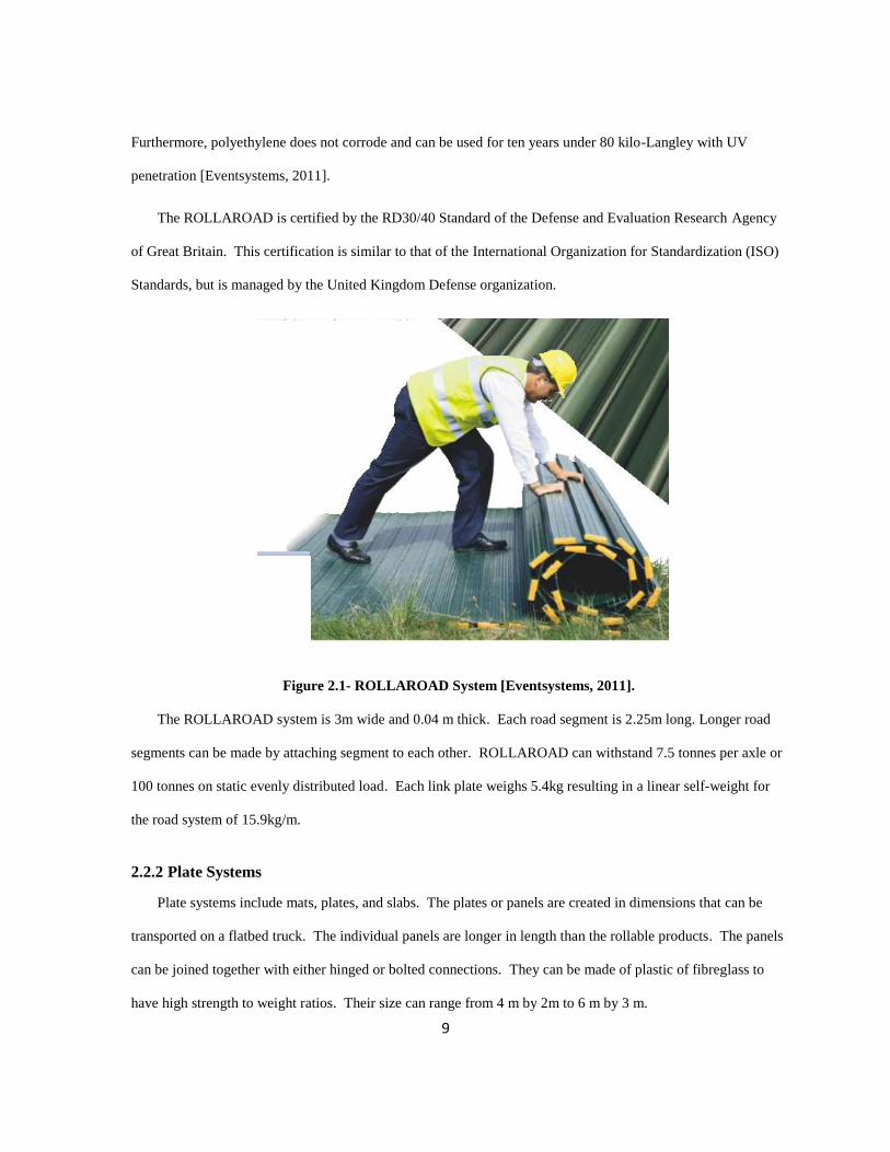
EventSystems [Eventsystems, 2011] is a company, which makes rolled products for ground protection, as
seen in Figure 2.1. The majority of their products are used for sports surfaces, such as stadiums and tennis
courts. Their PortaPath is a compacted version of the ROLLAROAD [Eventsystems, 2011] used to protect the
grass in stadiums for events, such as auto shows..
The ROLLAROAD system is a rolled mat system composed of high-density polyethylene. While other
materials were contemplated, polyethylene was chosen because it is 25% lighter and costs 50% less than
aluminum [Eventsystems, 2011]. Therefore, polyethylene has both advantages in regards to weight and cost.
9
Furthermore, polyethylene does not corrode and can be used for ten years under 80 kilo-Langley with UV
penetration [Eventsystems, 2011].
The ROLLAROAD is certified by the RD30/40 Standard of the Defense and Evaluation Research Agency
of Great Britain. This certification is similar to that of the International Organization for Standardization (ISO)
Standards, but is managed by the United Kingdom Defense organization.
Figure 2.1- ROLLAROAD System [Eventsystems, 2011].
The ROLLAROAD system is 3m wide and 0.04 m thick. Each road segment is 2.25m long. Longer road
segments can be made by attaching segment to each other. ROLLAROAD can withstand 7.5 tonnes per axle or
100 tonnes on static evenly distributed load. Each link plate weighs 5.4kg resulting in a linear self-weight for
the road system of 15.9kg/m.
2.2.2 Plate Systems
Plate systems include mats, plates, and slabs. The plates or panels are created in dimensions that can be
transported on a flatbed truck. The individual panels are longer in length than the rollable products. The panels
can be joined together with either hinged or bolted connections. They can be made of plastic of fibreglass to
have high strength to weight ratios. Their size can range from 4 m by 2m to 6 m by 3 m.

10
2.2.2.1 Hinged Plates
The majority of the hinged plate system use clasps that do not require bolts or rods to secure pieces of the
plate together (Figure 2.3) and still allow rotation between adjacent panels. Since there are no rods to connect
the plates together, lubrication is not required. Also, because the angle adjacent panels is normally small, a
complex hinge (allowing rotation about more than one axis) is not required
2.2.2.2 Canadian Mat System
The Canadian Mat System portrays the FiberCon [Canadian Mat System Inc., 2011] product as a
lightweight, non-absorptive, and high carrying capacity material. It is composed of a glass fibre reinforced
polymer (GFRP) or “fibreglass”, which is suggested to be stronger than wood [Ashby et al., 2007]. With
normal operating conditions, FiberCon can be used for 15 years. The mats by themselves are 50 mm in
thickness, as seen in Figure 2.2. Flexural modulus deals with the stiffness of the material, while the tensile
strength deals with the loading capacity base on material failure.
Figure 2.2 - FibreCon Product by Canadian Mat System [Canadian Mat System Inc., 2011].
One of the patented products by Canadian Mat System is a steel frame add-on to the FibreCon System that
allows for easy attachment and detachment of each panel. The C-Hinge does not require fasteners to create the
hinge connection. Therefore, one major advantage of this system is that it facilitates an ease of installation, as

11
well as quick turnover when the system is moved from site to site. The curve shape of the locking mechanism
prevents debris, such as mud, ice, and oil from accumulating.
Figure 2.3- C-Hinge System by Canadian Mat System [Canadian Mat System Inc., 2011].
One application of the FiberCon product with the steel frame is its common usage by many mining
companies, such as ESSO and Suncor, for staging platforms or construction roadways. It is used around the
world in places, such as Anchorage, Alaska and Jakarta, Indonesia [Canadian Mat System Inc., 2011]. The
platform system is 10 cm (four inches) thick with the steel frame. While the normal mat dimensions are 5.8 m
by 2.3 m and weighs 590 kg, there are other sizes for different applications. The International Organization for
Standardization (ISO) has specified dimensions for shipment of containers: 40 ’ (12.2 m) containers should
have dimensions of approximately 12.2 m by 2.4 m by 2.6 m [Murphy, 2009]. In an ISO shipping container,
thirty mats can be packaged. In an environment that lack soil support, i.e. the soil is in poor condition or there
is no support underneath, the mat can support 1.1 MPa (160 psi). In contrast, if strong soil is present, it can
support up to 4.1 MPa (600 psi). The other important consideration is moisture on the panel. A friction
coefficient of 0.92 is observed when wet and 0.88 when dry. Furthermore, this product is designed to perform
at a temperature range of -50oC to + 50
oC.
2.2.2.3 Bolted Plates
To reduce the complexity of the connections and improve the ridability of the roadway, some products
employ plates that are bolted together. When plates are bolted together, rotation is restrained and moments are

12
transferred from one plate to the next. While this results in higher load effects that must be carried by the joints,
it also results in a smoother surface and better ridability.
2.2.2.3.1 All Terrain Road
All Terrain Road (ATR) [All Terrain Road, 2005] has created a mat product that claimed to be extremely
light and portable. Each panel is composed of polypropylene in a honeycomb structure. ATR’s “direct energy
transfers” fasteners allow higher loading on the fasteners, as seen in Figure 2.4. The side of each mat is wedge-
shaped to allow room for expansion which is efficient for with standing large variations in temperature.
Figure 2.4- All Terrain Road System [All Terrain Road, 2005].
The ATR panels are used in urban construction sites, by natural resource industries, and for helicopter
landing pads. This mat product can also be used for a range of design conditions, such as over wetlands, ice
roads, and permafrost. Furthermore, these panels can be installed and removed quickly without truck-mounted
cranes.
Each mat only weighs 182 kg (400 lbs.) and can be placed, usually with the assistance of four individuals,
by hand. The mats are 2.31 m by 4.29 m (7.5 by 14 ft.). Since the mats are light, they easily transported as 112
13
mats can be carried on a 53 ft. trailer unit. In fact, the limiting factor of transportation is not weight, but height
restrictions.
2.3 Temporary Road Research
The published fundamental research on temporary road systems has primarily involved prototyping and
field testing with vehicles. Many of the road system testing and research has been conducted by the US Army
[Webster and Tingle, 1998] due to the need of rapid development of support roadways. The various
applications are described in the following sections.
[Webster and Tingle, 1998] report on test conducted to evaluate following five different types of
temporary road systems: fibreglass-reinforced, plastic hexagonal, aluminum hexagonal, non-reinforced plastic
mesh, and reinforced plastic mesh. The U.S. Military focuses on the comparison of the different systems rather
than the comparison of different thicknesses for a given system or different thicknesses for a givens system or
different soil properties. They conclude that the aluminum system performed the best because of the low rutting
that occurred during repeated load testing. Conversely, the plastic mats performed poorly because they
exhibited high rutting after minimal repeated loads. They tested both hinged and bolted designs which
discovered the bolted design in general can handle higher repeated loads. All the tested designs have a width
greater than that of the truck. Therefore, each individual segment supports both the left and right wheel loads
[Webster and Tingle, 1998].
[Gartrell, 2009] tested temporary tarmac systems on different soil strengths for aircraft applications. These
consist of mat systems designed for oil drilling work platforms made of high density polyethylene with insert
pins for a fixed connection, for construction to support heavy equipment over sand soils made of fibreglass with
insert pins, for foot traffic and light truck traffic made of plastics, for repairing damaged airfields, and for oil
industry for medium duty vehicles. The matting systems are either made of plastics, fibreglass, or aluminum.
These were tested with a vehicle mimicking a load of a C-130 aircraft. Rutting and damage per wheel pass
were recorded and compared. These values were also compared with the permanent plastic deformation limit
(7.2 cm) and number of failed connecting pins (20%) under the United States Air Force (USAF) criteria for

14
operations on contingency airfields. The products were tested under low (3-5 CBR), medium (8-10 CBR), and
high (40-50 CBR) strength soils. From his analysis, all the mat systems can support multiple aircraft loads
except for the mats which were designed for foot traffic. Products designed for heavy uses in the oil industry
preformed the best; these include mats made of fibreglass and metal.
[Fan et al., 2011] used equivalent cable theory to evaluate road mats. The research assumed rigid beam
behaviour for the individual mat segments. Hinged connections were assumed between the mat segments. The
model analysed the 2D impact of a vertical truck load. His formula can predict the mobility of vehicles on
hinged road mats. He suggested that lighter the vehicle, greater the adhesive force, stiffer the soils, and wider
and longer beams would help in the movement of the locomotive.
2.4 Existing Tools for Designing Modular Road Plate Systems
There are available tools and theories which can help design the modular road plate system. These theories
are not normally used within pavement designs. Terramechanics studies soil behaviour under dynamic loading
like farming equipment. Foundation design studies long term behaviour of soil under large loads. The next
sections will study the background and theories behind these tools, and their potential uses for the design of
modular road plate systems.
2.4.1 Terramechanics
Dr. M.G. Bekker [Bekker, 1974] pioneered off-road locomotion and the field of terramechanics.
Terramechanics is the study of soil interactions with mechanical devices. The following are two branches of
terramechanics: terrain-vehicle and terrain-implement mechanics. Terrain-vehicle mechanics refers to the
performance of the vehicle over unprepared terrain with respect to ride quality, handling, and manoeuvrability.
Terrain-implement mechanics refers to the efficiencies of terrain-working machinery to shape terrain as
required. In this section, terramechanics will refer solely to terrain-vehicle mechanics. The difference between
terramechanics and the road system is that the soils under the panels are not consistently shifting to the degree
of a wheeled or tracked off road vehicle.
15
[Wong, 2009] described the interactions of off road tracked and wheeled vehicles on weak or unknown
soil. This process allows for the analysis of the method by which agriculture vehicles work during operation.
This research advanced the defense designs and space explorations as it involved soil evaluation with elastic
and plastic behaviour. Before the concept of modern pavement, wheeled vehicles were driven on soils.
However, systematic studies on off-road vehicles were not significantly researched until the mid-20th
century.
Terramechanics of vehicles focus on the movement of soil after a vehicle has passed over it. The soil is
modelled both as a compressed medium and performance immediately following the loading. In most
applications, soil compression is overloaded, but soil sinkage is analyzed as applied to the agricultural industry.
In agriculture, soil is preferred not to be ‘yielded’ or ‘damaged’. Therefore, the elastic range of the soil is
analyzed. Within the road system design discussions, it is suggested that panels can be installed without
interference with the future usability of the soil because the road system would only be used as temporary.
Therefore, this section will discuss the disruption impact of the panels with soil support. In terramechanics, the
terrain is split between dense terrain, which could be compared with an ideal elastoplastic medium, and loose
terrain. In pavement design, vehicle contact dimensions for rigid pavement are modelled as an equivalent
rectangle.
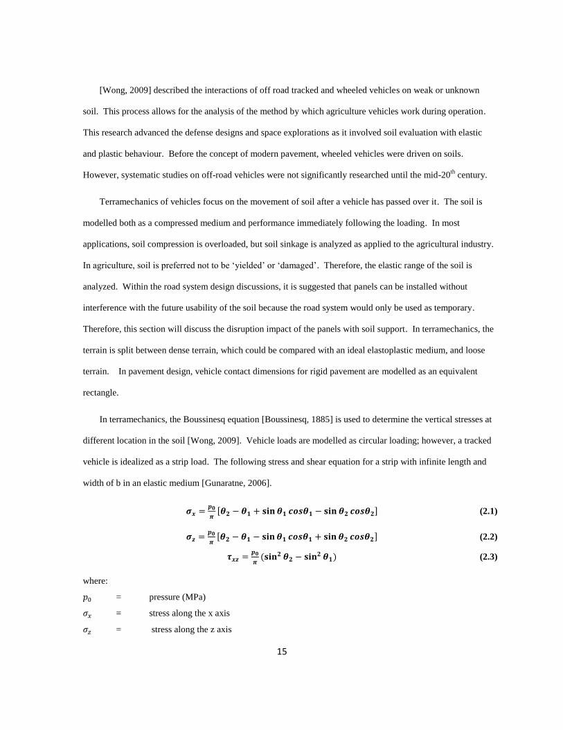
In terramechanics, the Boussinesq equation [Boussinesq, 1885] is used to determine the vertical stresses at
different location in the soil [Wong, 2009]. Vehicle loads are modelled as circular loading; however, a tracked
vehicle is idealized as a strip load. The following stress and shear equation for a strip with infinite length and
width of b in an elastic medium [Gunaratne, 2006].
(2.1)
(2.2)
(2.3)
where:
= pressure (MPa)
= stress along the x axis
= stress along the z axis

16
= shear stress perpendicular to x axis and along z axis
Figure 2.5- Boussinesq Equation Parameters. [Gunaratne, 2006].
With these set of equations, it is possible to determine the loading stresses within the elastic medium. With
the knowledge of the stresses in the calculated model, the accuracy can be assessed by comparing the finite
element model to the calculated model. By comparing stress from a soil contact size of a tire and a panel, the
resultant stresses can help classify the different finite element model as fully rigid supporting or fully flexible.
These ranges are the soil contact size of the tire contact and the panel size.
The Bekker pressure-sinkage equation [Bekker, 1974, Bekker, 1972, Bekker, 1966] determines the
deformation of the soil based on a pressure. The model uses a factor of 0.85 [Gunaratne, 2006] to compensate
for the differences in bearing pressure when comparing the flexible and rigid foundations.
(2.4)
and
= Bekker equation pressure-sinkage parameters
b = smaller dimension of the circular plate
z = sinkage
p = pressure
This equation can be used for rectangular plates of large aspect ratios in elastic mediums.
17
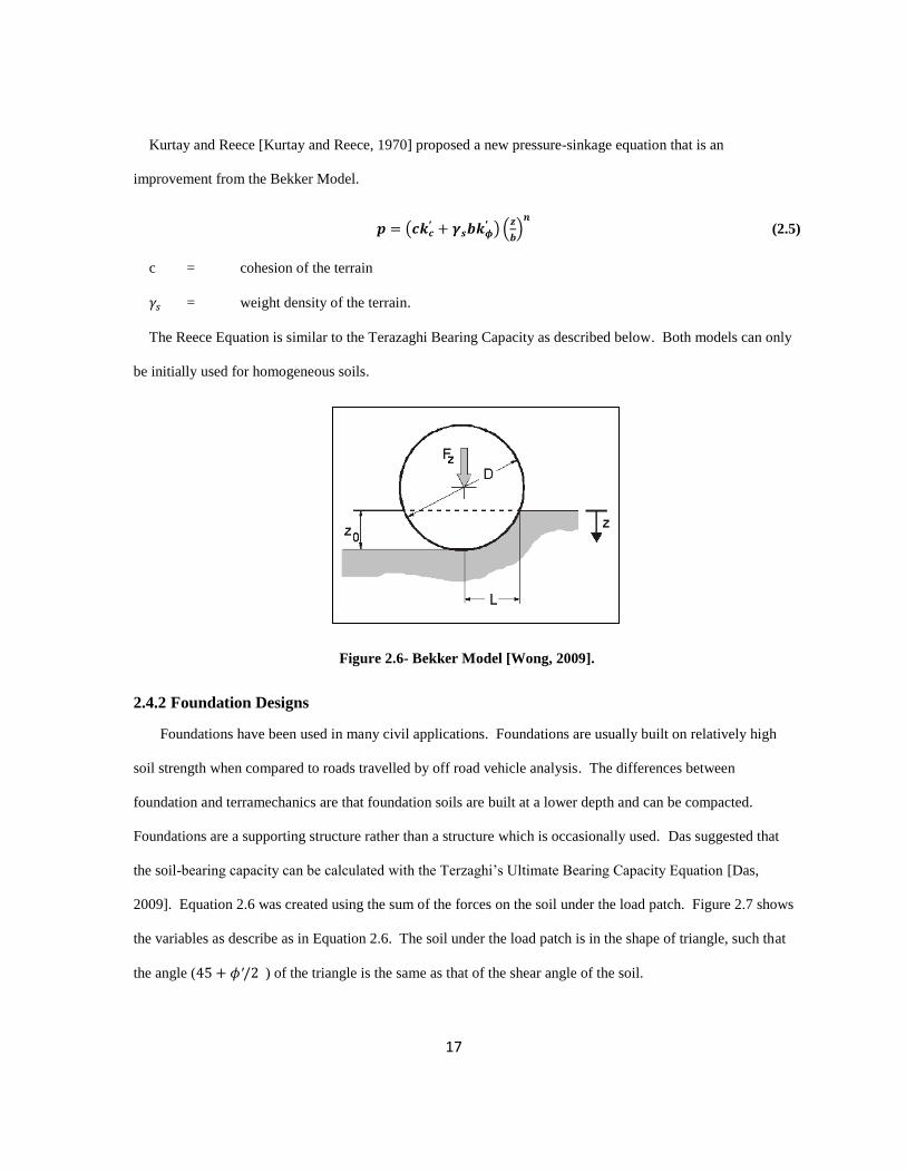
Kurtay and Reece [Kurtay and Reece, 1970] proposed a new pressure-sinkage equation that is an
improvement from the Bekker Model.
(2.5)
c = cohesion of the terrain
= weight density of the terrain.
The Reece Equation is similar to the Terazaghi Bearing Capacity as described below. Both models can only
be initially used for homogeneous soils.
Figure 2.6- Bekker Model [Wong, 2009].
2.4.2 Foundation Designs
Foundations have been used in many civil applications. Foundations are usually built on relatively high
soil strength when compared to roads travelled by off road vehicle analysis. The differences between
foundation and terramechanics are that foundation soils are built at a lower depth and can be compacted.
Foundations are a supporting structure rather than a structure which is occasionally used. Das suggested that
the soil-bearing capacity can be calculated with the Terzaghi’s Ultimate Bearing Capacity Equation [Das,
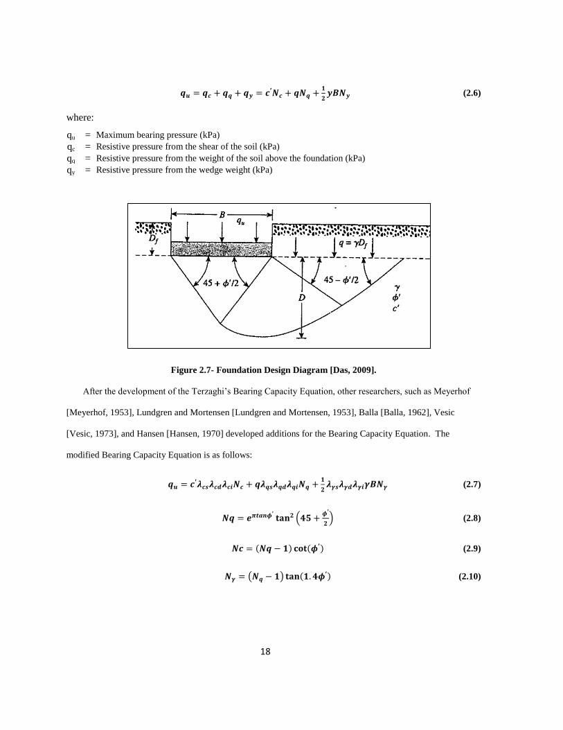
2009]. Equation 2.6 was created using the sum of the forces on the soil under the load patch. Figure 2.7 shows
the variables as describe as in Equation 2.6. The soil under the load patch is in the shape of triangle, such that
the angle ( ) of the triangle is the same as that of the shear angle of the soil.
18
(2.6)
where:
qu = Maximum bearing pressure (kPa)
qc = Resistive pressure from the shear of the soil (kPa)
qq = Resistive pressure from the weight of the soil above the foundation (kPa)
qy = Resistive pressure from the wedge weight (kPa)
Figure 2.7- Foundation Design Diagram [Das, 2009].
After the development of the Terzaghi’s Bearing Capacity Equation, other researchers, such as Meyerhof
[Meyerhof, 1953], Lundgren and Mortensen [Lundgren and Mortensen, 1953], Balla [Balla, 1962], Vesic
[Vesic, 1973], and Hansen [Hansen, 1970] developed additions for the Bearing Capacity Equation. The
modified Bearing Capacity Equation is as follows:
(2.7)
(2.8)
(2.9)
(2.10)
19
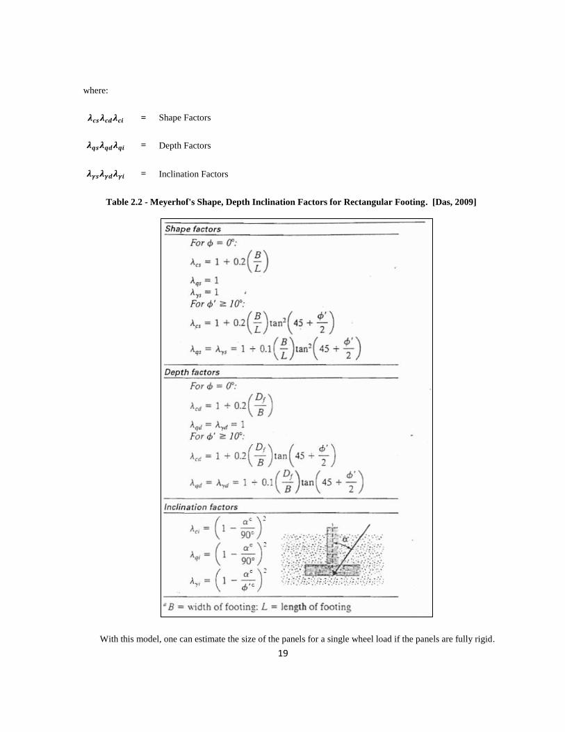
where:
= Shape Factors
= Depth Factors
= Inclination Factors
Table 2.2 - Meyerhof's Shape, Depth Inclination Factors for Rectangular Footing. [Das, 2009]
With this model, one can estimate the size of the panels for a single wheel load if the panels are fully rigid.

20
The Leaning Tower of Pisa is likely the most famous example of a loss in foundation. The loss of support
caused the tower to lean. It is possible to determine the stresses along the plane of the soil using fundamental
principles of the mechanics of deformable solids. Using Boussinesq’s equation, [Boussinesq, 1885] the
following calculations are of the vertical stresses under the corner of the flexible rectangular load:
(2.11)
(2.12)
(2.13)
(2.14)
where:
= Stress in the z axle at ‘z’ distance from the surface (Pa)
z = distance from the bottom surface of the load (m)
L = length of the load area (m)
B = width of the load area (m)
The last model only calculates the corner stresses under the load area using the previous equations:
(2.15)
(2.16)
(2.17)
(2.18)
where:
z = distance from the bottom surface of the load (m)
L = length of the load area (m)
B = width of the load area (m)
The Bearing Capacity Model analyzes the failure of soil during loading. The model demonstrates the
appropriate force for a certain soil condition and load area. Because this model is derived from the
21
Boussinesq’s equation for point load, the medium is assumed homogenous. However, soils are not
homogeneous or perfectly elastic. Therefore, there may be inconsistencies between the theoretical models and
the actual values. The differences between the two values are ± 25 to 30% [Das, 2009]. Since models in this
thesis will use perfectly elastic soils, this theory will be used to compare with these models.
2.4.3 Finite Element (FE) Analysis
Finite element method (FEM) is a set of numerical calculation to find approximate solutions to the model
system. Combining functions of physical models, like Hooke’s law, from small parts of the model can create a
larger set of equation to define the model. Able to use no linear or dynamic functions is one of the advantages
of this method. With the complexity of mechanistic approach with respect to geometry, non-homogenous
material, and non-linear materials, it would be more efficient to use computer software that iterates the
calculations. This program recognizes that each material has individual variables, instead of assessing them
together as one. It is, therefore, challenging to analyze non-linear stress-strain relationships in the context of
pavement design. With the finite element method, non-linear relationships in elastic and plastic regions of the
material can be used in the calculations.
There are finite element programs that are specific for pavement consisting of slabs. KENSLABS [Huang,
1993] uses the vertical concentrated force from the wheel loads and subgrade reactions. The program uses
different types of foundations and slabs. The options include: liquid, solid, and layered foundations. Liquid
foundation models are used in the Winkler foundation, which is characterized by an elastic spring [Gunaratne,
2006]. The word “liquid” is specified because the relationship between a spring and a floating boat; where the
force from the underside of the boat is from the buoyancy of the boat; is based on the weight of water from
which the boat is displaced. In solid foundations, the stresses within the foundations are uniformly distributed.
The Boussinesq equation [Boussinesq, 1885] is a representation of this type of foundation. The Boussinesq
equation was be described in an earlier section (Equation 2.1). Slab to subgrade are concrete pavement slabs
which rest on the subgrade. These slabs can be modelled as either bounded or unbounded to the subgrade. The
calculations for bonded slabs are similar to a compound slab or beam in a structural application. The composite
moment of inertia is calculated according to the neutral axis of effective width. When the slabs are unbounded,

22
the stiffness matrix is added together. When the displacement is determined, the moments for each node are
calculated.
Abaqus has been used in many engineering applications as a finite element program. It can calculate
physical forces, thermal interactions, and acoustics. In pavement analysis, Abaqus has been used to model
pavement behaviour in repeated loading [Uzarowski, 2006] and joint analysis [Prabhu et al., 2009].
Models can be simplified by changing the beam elements into a shell element [Robinson et al., 2011].
Their research states that it is suitable to reduce solid to shell elements when the length is relatively long
compared to the thickness. Because of the thickness to length ratio, it is not efficient to create a mesh to
correlate with actual physical attributes for the allotted computational time. Danielson [Danielson et al., 1996]
suggests that during the finite analysis of a tire in contact with pavement, it is appropriate to model half of the
tire with the appropriate cross symmetry. Both researchers suggested that a poorly meshed shell element is
more accurate than a poorly meshed solid element when the length verses thickness ratio is small.
2.5 Summary of Findings
Section 2.1 discussed how conventional roads ways are designed with either asphalt or concrete materials.
Conventional design process does not allow for alternative materials like metals or polymers. Section 2.2
uncovers the different available temporary road or platform products which are commercially used. There is no
extensive development in making the products efficient for different soil conditions. Section 2.3 highlights the
ongoing researches of temporary roadways. These researches are mostly military funded to test current
products for their durability. Section 2.4 gathers different theories from foundation design and terramechanics.
These theories can be implemented to support this research.

23
Chapter 3
Design Criteria
In the following sections, design criteria for a modular road plate system are discussed and proposed. In
Section 3.1, the main performance aspects are discussed, including: structural capacity to resist vertical and
horizontal traffic-induced loads, and skid resistance. In Section 3.2, initial to final costs are broken down and
analysed. In Section 3.3 discusses the durability factors that can create a system that can last. This section also
introduces which materials are advised to be used in long term roadways. Section 3.4 shows what kind of
methodology will be used to design such systems. This will sum up the performance, cost, and durability
within the design process. Section 3.5 will introduce the limits and requirements. These limits will include
both objective limits, such as material failures, and subjective limits, such as ridability.
3.1 Performance
A modular road plate system is expected to provide stable vertical support for the safe passage of traffic
passing over the road way, while protecting the ground below from damage during the service period. In order
to perform this function, the following system performance requirements have been identified: 1) adequate
structural capacity to resist vertical traffic loads, 2) adequate structural capacity to resist horizontal traffic loads
(i.e. braking or centrifugal forces), and 3) adequate skid resistance of the road plate surface.
The road is designed to carry the identified loads over varying environment conditions. On initial soil
loading, the soil behaves as an elastic medium [Das, 2009]. Therefore, it is appropriate to model the road
system with elastic support. The quality of the pavement will be directed related to a material performance.
The material will be analyzed for yielding when failure occurs because the road system is not a single-use
system.
3.1.1 Structural: Vertical Loads
On a conventional roadway, vehicle-induced vertical loads can vary considerably, depending on the type
and quantity of goods being carried. For each vehicle, the load distribution between axles will also vary
depending on the number of axles and their arrangement. In the design of highway structures such as bridges,

24
the axle loads due to automobiles are generally ignored, as they are much lower than the truck axle loads. For
bridges, truck wheel loads can be modelled as uniformly distributed or concentrated loads. For modelling the
local behaviour of smaller components, the latter approach is more appropriate.
Truck/axle loads can be modelled as single axles with single tires, single axles with dual tires, and tandem
axles with dual tires [Huang, 1993]. A possible assumption for the tire spacing can be seen in Figure 3.1. With
this type of loading procedure, the distance between the axles is too large for the load of each axle to be
dependent. In flexible pavement design, wheels along only one side of the vehicle are considered, while the
wheels on both sides are considered in rigid pavement design.
The Equivalent Single Axle Load (ESAL) is used to provide a measure of load by combining the mixed truck
traffic into an equivalent number for design purposes. In AASHTO Pavement Design Guide [American
Association of State Highway and Transportation Officials1993], an 80 kN-load single axle is used for
highways designs. ESAL’s are often based on site recordings on site or calculated based on certain
assumptions. AASHTO Design Guide allows for mix traffic to be calculated to an ESAL. This is done by
applying equivalent axle load factor (EALF) on axle loads which are higher and lower than the 18 kips axle
load. For example, with a terminal serviceability of 2.5 and a structural number of 5.0, a truck with a single
axle weight of 10 kips would be 8.8% of the truck count. Structural number is calculated by the thickness,
modulus, and drainage conditions of the base and subbase. Terminal Serviceability is the condition of
pavement which is considered to have failed. By putting all the mix traffic into Equivalent Single Axle Load of
18 kips.
where:
m = number of axle group
Fi= EALF for the ith
axle group
n = number of passes of the ith
axle group

25
The contact area of the tire depends on the contact pressure. The contact pressure of a low pressure tire
would be higher than the tire pressure because the walls of the tires are compressed, and therefore increasing the
contact pressure. The opposite is true when the tire is in over-pressured. The contact pressure would typically
be less than the tire pressure because of the tension in the tire material. Also, it is possible for inflated tires to
differ 10-15% in pressure due to different temperatures [Mallick and El-Korchi, 2009]. Actual tire pressure is
non-uniform on the contact area. If the tire is underinflated, the edge of the tire will have higher pressure.
Moreover, if the tire is over inflated, the centre of the tire will have higher pressure. However, this physical
attribute is not typically considered in current pavement design practice [Huang, 1993]. For design purposes,
contact pressure if often simply assumed to be equal to the tire pressure. Vehicle tire pressure can range from
50 – 100 psi (345 – 690 kPa) [Young et al., 2004]. With the current practice of replacing dual wheel axles with
super-single tires, there will be an increase stresses in the pavement by 10 - 35% because of the higher pressures
required for those tires [Greene et al., 2010]. Super-single tires reduce fuel consumption based on rolling
resistance [Ioannides, 1992].
Figure 3.1- Wheel location for pavement thickness calculations [Huang, 1993].
A design truckload of 625 kN (140 kip) is specified in the Canadian Highway Bridge Design Code [Canadian
Standards Association, 2006] in Figure 3.2. A 625 kN design truck with a slightly different axle arrangement is
used in Ontario (see Figure 3.3). For either design truck, the maximum wheel load is 87.5 kN (20 kip).
Since a modular road plate system is something in between a pavement and structural component, good
arguments could be made for designing it using either the existing pavement or bridge code models. For the
current study, it was elected to use the CL-625-ONT wheel, axle, and truck loads for modular road plate system

26
design. This model was chosen, since it is representative of Canadian truck traffic and enables analysis under
multiple wheel or axle groups. With a tire contact area of 250 mm by 600 mm, as specified in Figure 3.3, and a
maximum wheel load of 87.5 kN, the contact pressure is 0.5833 MPa (84 psi), which falls within the range
suggested by [Young et al., 2004]. The effects of varying this assumption (e.g. to model road plate use with
load restrictions or in industry sector applications) are not investigated.
Figure 3.2-CL-W Truck Load Diagram [Canadian Standards Association, 2006].
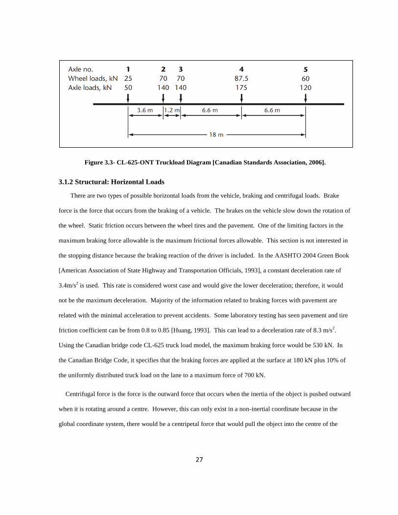
27
Figure 3.3- CL-625-ONT Truckload Diagram [Canadian Standards Association, 2006].
3.1.2 Structural: Horizontal Loads
There are two types of possible horizontal loads from the vehicle, braking and centrifugal loads. Brake
force is the force that occurs from the braking of a vehicle. The brakes on the vehicle slow down the rotation of
the wheel. Static friction occurs between the wheel tires and the pavement. One of the limiting factors in the
maximum braking force allowable is the maximum frictional forces allowable. This section is not interested in
the stopping distance because the braking reaction of the driver is included. In the AASHTO 2004 Green Book
[American Association of State Highway and Transportation Officials, 1993], a constant deceleration rate of
3.4m/s2 is used. This rate is considered worst case and would give the lower deceleration; therefore, it would
not be the maximum deceleration. Majority of the information related to braking forces with pavement are
related with the minimal acceleration to prevent accidents. Some laboratory testing has seen pavement and tire
friction coefficient can be from 0.8 to 0.85 [Huang, 1993]. This can lead to a deceleration rate of 8.3 m/s2.
Using the Canadian bridge code CL-625 truck load model, the maximum braking force would be 530 kN. In
the Canadian Bridge Code, it specifies that the braking forces are applied at the surface at 180 kN plus 10% of
the uniformly distributed truck load on the lane to a maximum force of 700 kN.
Centrifugal force is the force is the outward force that occurs when the inertia of the object is pushed outward
when it is rotating around a centre. However, this can only exist in a non-inertial coordinate because in the
global coordinate system, there would be a centripetal force that would pull the object into the centre of the

28
radius. There is a relationship between the force that the object sees, velocity of the object, and radius of the
turn.
(3.1)
where:
F= centrifugal force
m = mass
v = velocity
r = radius
In the pavement code, the curvature and speed of the vehicle pertain to the ability for the vehicle to stay on
the pavement, but not the forces created by the turning vehicle on the pavement. In the Canadian bridge code,
mass is taken as CL-W Truck load divided by a factor of 127. This force is applied as a right angle to the
direction of travel and 2.0 m above the deck surface. This would create both a horizontal force and a moment
within the pavement, which would create an uplift force at one of the edges. The frictional forces can also
deduce the maximum possible centrifuge forces because once the vehicle turns to sharp or increases it speed in
a turn, it would slip.
3.1.3 Skid Resistance
Skid resistance is very closely related to the braking forces. A proper skid resistance allows the vehicle to
stop in time during an emergency to prevent an accident. Skid resistance is more important during wet weather
because water would decrease the friction between the tire and the pavement. Keeping proper skid resistance
requires proper texture and drainage in the pavement. Drainage can be inhibited by lack of grade or sunken part
of the pavement, like rutting. Proper texture is attributed by aggregate types and size, mixture proportion, and
texture orientation and detail [Transportation Association of Canada, 2012]. To test these panels for skid
resistance, there are possible field and lab test. In the field, the portable skid resistance tester (Pendulum tester)
is used by swinging a pendulum with a rubber end. As the rubber contacts the pavement, energy from the
falling pendulum is absorbed. The remaining energy is captured at the upswing of the pendulum. Road,
Pavement Friction Tester is a more automated friction tester where an extra wheel vehicle or trailer is locked to
29
record static friction. In the lab, Asphalt Mix Design tests if a mixture of asphalt pavement has appropriate skid
resistance [Transportation Association of Canada, 2012].
3.2 Cost
The total costs of a modular road plate system can be broken down into: initial, manufacturing, installation,
maintenance, and decommission cost. In conventional pavement design, initial and installation costs are
generally combined with the construction or manufacturing cost. However, the proposed modular road plate
system can be installed multiple times. The more times the system can be reused, the greater the chance of
recuperating the higher initial cost of fabrication
The initial cost accounts for the costs of manufacturing the system. Optimizing the design is critical for
minimizing the initial material and fabrication costs. For example, considering a simple plate system with a
plate thickness of 20 mm, if this thickness can be decreased by 1 mm, then the material cost can be decreased
by five percent. This would be a significant reduction in the material cost. However, the fabrication (e.g.
machining) cost may not be lowered. Considering that the road system may be longer than 1 km, it is an
important cost saving factor to calculate the minimal required thickness. Unlike most temporary road products
in the market, the panel thicknesses are not optimized for the locations where they will be used. The design is
intended to be multifunctional for usage in many situations. This concept may be valid for the design because
the panels are used in multiple location types with minimal time frame. Over the product life cycle, it may be
used in locations of strong and/or weak soils. Therefore, it may be appropriate to design this product to
withstand all failures modes for a variety of different design scenarios. The opposite is true for conventional
pavements, where pavement costs are optimized for the location expected depending on traffic and
environmental loads for the given design scenario.
With that design concept, the product is required to withstand all failure criteria. There are two ways to
approach the design criteria: 1) have one design for all range of soils or 2) have multiple designs for different
soil scenarios. For the first approach, as the panels are design for different scenarios, the manufacturing cost
increase because of the design limitations. The design may work for the weakest support, but is over designed

30
for a strong support. For the second approach, if the panels are only design for one scenario, similar to what
conventional pavement, the reusability of the panel would not be feasible. To allow for different scenarios for
the given panels, its dimensions may be different for a variety of locations and sites which would increase
engineering cost. It is not economically feasible to design and build panels which are used for only one type of
soil condition. If these panels are designed to be reusable, being specifically designed for only one location may
limits its usage. Also, increasing the types of panels available would increase the cost associated for building.
Therefore, a proper balance of the design criteria would decrease the cost of engineering and manufacture of the
plate system. Also, it may be necessary to enhance the soil at the location to fit into the proper limits of the
panels. Having more variety of panels may be more economical for the user, but not for the manufacturer. It is
not economically feasible to design and build panels which are used for only one type of soil condition. If these
panels are designed to be reusable, being specifically designed for only one location may limit its usage. Also,
increasing the types of panels available would increase the cost associated with construction. In determining
whether a “one size fits all” solution or a range of designs for different soil or loading conditions would work
best, the concept of “returns to scale” [Frisch and Christophersen, 1964] becomes relevant, wherein
proportionality between input and output changes is assumed. When this proportion is linear, this is referred to
as “constant returns to scale”. When the outputs increase less than the rate of the input, this is referred to as
“decreasing returns to scale”. In the current context, when more choices are offered, there may not be an
increase in demand because the product still serves the same number of customers. However, this increase in
choices also increases in the cost associated with design and manufacturing. Because of economy of scale
[Gunaratne, 2006], localizing the initial built can decrease the cost per unit. These saving may be caused by the
discount by purchasing in bulk and efficiency of the manufacturing.
Installation costs includes of shipping, labour, and any other cost associated with installation that cannot be
reused. Equipment costs for installation may be lower than for regular pavement because (depending on the
final modular road system design) there may be no need for specific pavement laying equipment. The major
equipment required for the modular road plate system would be a lift or crane to place the panels (if they are too
heavy to be lifted by hand) and any equipment required to connect the panels. The maintenance costs include

31
the time, labour, equipment, and materials required to replace damaged panels or remove them when the road is
no longer needed. The time needed to replace the panels is similar to installation of the panels. Disposal costs
may be positive or negative depending on the recyclability of the material, and could vary if the panel damage is
minimal enough for repurposing. The decommissioning costs include all of the cost associated with the
dismantling of the panel roadway and the cost of restocking the panels at a storage location.
The costs discussed in the previous paragraphs can all be attributed to the owner of the modular road plate
system (whether it is a government body, a private agency, or a contractor). There are also indirect costs
associated with roads that can be attributed to the user. In terms of pavement usage for a public road, the loss of
time is a cost paid by the user and often referred to as the user delay cost. This can also be considered as an
opportunity cost for the traveler, based on the value of traveller’s time. These costs can be particularly
burdensome when the project operates for extended periods of time [Transportation Association of Canada,
2012]. The World Bank [Archondo-Callao and Faiz, 1994] uses a road user costs model, which analyzes twelve
different types of vehicles and considers the following user costs: operating cost, time cost, accident cost, and
emissions. Using this model, road user cost can be calculated. Furthermore, there are costs associated with the
owner if it is a private road. These costs are related to the time that is required to build the road. The costs can
vary depending on the company’s ability to plan for the construction of the roads ways based on their current
processes and the usage of the roadway.
3.3 Durability
Durability of the system depends on the mechanical behaviour and material selection. . Designing the
product to have good durability would mean it can be reused more times to recuperate the initial fabrication
cost. There are a wide range of deterioration mechanisms that can limit the service lives of mechanical
components. These include: corrosion, fatigue, and photo-degradation..
Certain metals are particularly susceptible to corrosion. Certain metals are particularly susceptible to
corrosion. Corrosion occurs when the metals is dissociated into ions and releasing electrons. Metals which are
corroded often turn into different forms of metal oxides. For example, iron metal in water can dissociate into

32
iron ion which turns into iron oxide when in contact of water and air. Some alloys only require being exposure
to moisture in the air [Ashby et al., 2007]. Within the operating parameters, these panels will be within the
natural pavement environment, which consist of air, moisture, and salts [Transportation Association of Canada,
2012]. Corroded areas can decrease the stress capacity around the area because the corroded material offers no
structural support. Also, these areas are more susceptible to fatigue because it creates area where cracks can
form.
To mitigate corrosion, corrosion resistant metals or non-metallic materials can be selected, or corrosion
susceptible metals can be protected with coatings. Non corrosive metals, such as platinum and gold, resist
corrosion because of their high electro-negativities to prevent from becoming ions. Non-metallic materials,
such as carbine fibre and plastic, do not corrode. Metals can be coated naturally or industrial to prevent
corrosion. Natural coating, such as aluminum oxide, is a passive layer created by the original aluminum metals
and will prevent the aluminum metal from further corrosion. An industrial coating, such as zinc, uses it as a
sacrificial layer which to prevent the corrosion of the main metal. Designs should not use dissimilar metals in
connections. For example, using a copper bolt to connection two steel plates would localize the corrosion on
the steel around the bolt. Adding a sacrificial anode to the metal can help protect the actual metal. For
example, a piece of steel coated with zinc will be protected because the corrosion will first occur on the zinc.
Common processes for doing this are galvanizing and metalizing. A polymer film can also be applied to
prevent any moisture contacting the metal.
Fatigue is a type of failure mechanism that occurs with repetitive stress cycles that are not above the yield
point. During fatigue loading, cracks are initiated in the material as the result of plastic slip along shear planes
near the surface of the material. To mitigate fatigue failure, designs must account for the endurance limit of the
material, which is a measure of the material’s resistance to crack initiation. Minimizing sharp changes in
geometry or material defects can also improve fatigue performance by reducing or eliminating local stress
concentrations. Surface treatments (e.g. peening) to introduce compressive residual stresses (which inhibit crack
growth) are another way to improve the fatigue performance of mechanical components.

33
Another degradation mechanism is photo-degradation. This mechanism is more prevalent in polymers when
exposed to light and oxygen. It can cause decrease in strength, stiffness, and coloring. To combat photo-
degradation, additives, such as antioxidants, light stabilizers, or fluorescent whitening agents can be used
[Ashby et al., 2007]. The amount of additives needed is dependent on the operating conditions like daily
sunlight amount and temperature ranges. Not only polymers but fibre-reinforced composite materials where
polymers comprise the fibre or the matrix are also susceptible to this form of degradation.
3.4 Research Methodology for Vertical Load Design
Given the performance, cost, and durability requirements for a modular road plate system described in the
previous sections and the available tools described in Chapter 2 (currently used for pavement design or well-
suited for designing modular roads), a methodology was established as part of the current project, for the design
of modular road plate systems. This methodology is summarized in Figure 3.4. In this figure, a single material
panel with predefined plan dimensions is assumed. Simple modifications would be required to extend this
methodology to composite systems with different plan dimensions. The proposed design methodology is limited
to the establishment of a suitable plate thickness to resist the vertical loads due to the passage of vehicular
traffic. The other performance criteria discussed in Section 3.1 (horizontal load and skid resistance) would also
need to be considered in the complete design of a modular road plate system.
To determine the minimum thickness requirement for the panel system, a number of inputs need to be
defined. These inputs include: the ranges of loading conditions and subgrade properties that the fabricated
system is expected to see during its service life. The inputs are either constant (i.e. panel material strength) or
variable (i.e. trial thicknesses as described later in Section 4.3 and soil conditions described in Section 3.5.1).
The different trial scenarios can be used to establish a range of conditions for which a given panel thickness
would provide a satisfactory design.

34
Figure 3.4- Research Methodology.
3.5 Material Properties and Limits for Vertical Traffic Load Design
3.5.1 Road Plate: Material Properties and Strength Limits
Steel was used in the initial design process because it is easy to model and can be applied easily on the
field. The steel properties used are similar to the ones which are used in structural codes because they have
proven to their characteristics. In the Canadian Highway Bridge Design Code [Canadian Standards
Association, 2006], structural steel is taken to have an elastic modulus of 200,000 MPa and shear modulus of
elasticity of 77000 MPa. The yield strength of structural steel can range from 200 to 500 MPa [Ashby et al.,
Initial Design Development Methodology
Traffic Subgrade Properties
Trial Pavement Thicknesses
Trial Soil Subgrade Modulus
Structural Analysis
Sensitivity Analysis
Soil Dimensions Mesh of System
Panel Material Strength(Material Yield Limit)
Deformation Limit(Pavement Code and Ridability Research)
Soil Bearing Capacity(Soil Bearing Failure)
Minimium Design Requirement

35
2007]. Atmospheric corrosion-resistant steel will be used in this process. These steel have yield strength of
350 MPa and have a minimal thickness of 1/2 inch (12.7 mm)
3.5.2 Soil: Material Properties and Strength Limits
The modular road plate system must not fail under short term loading. Under short term loading, the soil
behaves as an elastic medium [Das, 2009]. Therefore, it is appropriate to model the road system with elastic
material properties assumed for the subgrade.
Soil can be classified into a range of soil types [Gerrard, 2000]. The material property ranges for the
different soil types can be used to establish trial soil properties for use in the proposed vertical load design
methodology. The modular road plate system would offer the greatest advantage over conventional pavement if
it can be installed with little or no subgrade preparation. For very weak soils, however, subbase should be added
to enhance the stiffness bearing capacity of the soil.
Modulus of subgrade reaction is an equivalent soil material property of the spring constant of Hooke’s
Law, while soil bearing capacity is the strength of the material [Das, 2009]. There is no direct correlation
between those material constants. Modulus of subgrade reaction or elastic modulus of the soil focuses on the
temporary loading response of the soil, while soil bearing capacity is associated with large deformations.
Modulus of subgrade reaction can be used if deformations are low. In the AASHTO Design Guide, modulus of
subgrade reaction (k) can be related to soil elastic modulus (E) with the following equation.
(3.2)
where:
= Modulus of subgrade reaction (MPa)
= Elastic Modulus (MPa)
In Table 3.1, soil elastic modulus ranges are shown for clay and sand.

36
Table 3.1- Ranges of soil elastic modulus for different types of soils.
Soil Elastic Modulus (MPa)
Clay Very Soft 0.5 - 5 Soft 5 - 20
Medium 20 - 50
Stiff, silty 50 - 100
Sandy 25 - 200 Shale 100 - 200 Sand
Loose 10 - 25 Dense 25 - 100 Dense with Gravel 100 - 200
Silty 25 - 200 In Terzaghi’s Bearing Capacity (in section 2.4.2), bearing capacity can be a model varied by different slip
angles of soil. The soil modulus and bearing capacity assume that the soil has no cohesion. As such, the
following bearing capacity can be shown with a footprint size of 1 m by 1 m panel contact or 0.6 m by 0.25 m
wheel contact.
As shown in Table 3.2, the maximum allowable load for an 87 kN vehicle is for a slip angle of 42 degrees
for a direct wheel in surface contact and 28 degrees for a rigid panel to surface. Combining Table 3.1 and Table
3.2, the critical strength for soil can be found to limit the constraints of the future finite element models. These
calculations can aid in the design of the size of the panel requirements such that the final concepts should be
able to handle loads between those soil properties. The data for Table 3.2 is shown on Figure 3.5.

37
Table 3.2- Maximum Allow Load for different Slip Angle with Bearing Capacity Equation.
Theta
(θ)
Maximum allowable Pressure (kPa) Maximum allowable load (kN)
Wheel Contact Panel Contact Wheel Contact Panel Contact
20 15.63 26.05 2.34 26.05
22 22.14 36.90 3.32 36.90
24 31.12 51.87 4.67 51.87
26 43.57 72.62 6.54 72.62
28 60.92 101.54 9.14 101.54
30 85.31 142.18 12.80 142.18
32 119.90 199.84 17.99 199.84
34 169.57 282.62 25.44 282.62
36 241.88 403.13 36.28 403.13
38 348.85 581.42 52.33 581.42
40 510.10 850.17 76.52 850.17
42 758.52 1264.20 113.78 1264.20
44 1151.02 1918.37 172.65 1918.37
46 1789.79 2982.99 268.47 2982.99
48 3065.55 4999.45 459.83 4999.45
50 5291.51 8567.70 793.73 8567.70
Figure 3.5- Maximum Allow Load for different Slip Angle with Bearing Capacity Equation.
0
1000
2000
3000
4000
5000
6000
7000
8000
9000
1
10
100
1000
10000
20 22 24 26 28 30 32 34 36 38 40 42 44 46 48 50
Load
Fo
rce
kN
Pre
ssu
re (
MP
a)
Soi Slip Angle (degrees)
Pressure of Wheel Contact
Pressure of Panel Contact
Load of Panel Contact
Load of Wheel Contact

38
3.5.3 Vertical Deformation Limits
The Pavement Quality Index (PQI) is used widely to rate pavement performance. It maps the deterioration
and predicts when maintenance is required. It is a combination of the Riding Comfort Index (RCI), the
Structural Adequacy Index (SAI), and the Surface Distress Index (SDI). It is calculated as follows:
(3.3)
Ride quality is a measure of the passengers’ comfort while riding. However, there is equipment to measure
the roughness of pavement using both indirect and direct methods. Indirect measurement refers to the change of
distance using optics. This profiles the road as different heights and derives an overall Roughness Index. The
direct measurement uses an independent wheel to analyze the actual response of the wheel to the vehicle by
measuring acceleration. Also, the APL Profilometer is a single wheel instrument with a horizontal pendulum to
determine the inertia and the angle difference from a reference plane. The direct measurements are sensitive to
speed. Therefore, any instrument using that procedure is required to take measurements at a constant speed.
The MTO’s Manual for Condition Rating for Rigid Pavement [Chong and Wrong, 1995] discusses the
process for pavement evaluation. According to this reference, pavement is evaluated based on the following
attributes: ride quality, distress manifestation, surface defects, surface deformations, joint deficiencies, and
cracking.
The design uses objective numbers to define a relatively subjective scale. Of the types of defects, only
potholing and faulting (stepping) result in surface height differences that might influence ridability, as seen in
Table 3.3.
Table 3.3- Different Severity Classes Description for Potholes and Faults.
Class Potholing Faulting
Very Slight Barely noticeable Less than 3 mm
Slight Disintegration of surrounding material 3 – 6 mm
Moderate Wider than coarse aggregate and less
than 75 mm
7 – 12 mm
Severe 75 – 150 mm deep 13 – 19 mm
Very Severe Over 150 mm deep More than 19 mm

39
Potholes are depressions in the pavement surface and are independent of cracking and joint defects. They
result from fatigue of the road surface. Oversized particles of soft aggregates and placement of the reinforcing
steel too close to the surface can cause potholes. Potholes manifest because of water seepage into the pavement
surface and loosening the pavement structure. Faulting is a difference in vertical displacement between
adjacent slabs at joints in the pavement, as seen by Figure 3.6. This is resulted from the loss of subgrade,
pumping under the slab, or freeze-thaw cycles. In the case of transverse faulting, the elevation of trailing slab is
usually higher than the leading slab because force on the leading slab is more sudden. Due to the higher force
and displacement of the leading slab edge, slab will pump water and subgrade soil the adjacent slab. With the
loss of subgrade, the edge of the leading slab will permanently deform downward, while the trailing slab edge
will deform upwards. The resulting permanent deformation will lead to cracking at some distance from the
joint.
Figure 3.6- Pumping of Rigid Pavement [Huang, 1993].
The limited deflection method involves correlation of the vertical deflections and the required thickness of
the pavement. Kansas State Highway Commission [Keeling, 1947] modified Boussinesq’s Equation
[Boussinesq, 1885] and limited the deflection of the subgrade to 0.1 in (2.54 mm). The U.S. Navy [Lynch
et al., 1999] referred to this as the Burmister’s two-layer theory [Burmister et al., 1943] and limited the
deflection of the surface to 0.25 in. (6.35 mm). This limited deflection method is popular with field analysis
because it is easy to take deflection data as a predicting variable for pavement maintenance. However,

40
pavement failures are not caused by deflection, but from stresses and strains that exceed the structural design.
Caution should be used when relating limited deflection with current pavement design because concrete and
asphalt are more prone to low flexural strength. In the Canadian Highway Bridge Design Code, a serviceability
limit decreases the discomfort or concern of users of the bridge [Canadian Standards Association, 2006]. These
limits are based on frequency and static deflection at the sidewalk or inside face of the barrier. The limit can
range from a maximum allowable deflection of 200 mm for a frequency of 1 Hz to 7.5 mm for a frequency of
10 Hz if there are no pedestrians.
Figure 3.7 – Deflection Limits for Highway Bridge Superstructure Vibration [Canadian Standards
Association, 2006]
3.6 Summary of Key Findings
This chapter focused on the design constrained, which are performance (Section 0), cost (Section 3.1.2),
and durability (Section 3.3). In performance, the appropriate load was described in accordance to current
roadway building codes. Cost constraints are characterized as construction and time cost. Cost can increase

41
drastically even if there is a small delay in construction. Durability focused on the failure mechanism of
degradation and fatigue. Section 3.4 describes the research methods while incorporate material properties to
design constraints to find appropriate thickness. Section 3.5 shows the appropriate numerical limits based on
soil properties and displacement, which is related to ultimate limit state and serviceability limit state
respectively.

42
Chapter 4
Design Concepts
In the following chapter, the various materials that could be used in the fabrication a modular road plate
system, and the advantages and disadvantages of these materials are discussed in Section 4.1. Following this,
in Section 4.2, several modular road plate system design concepts are discussed and evaluated qualitatively. In
Section 4.3, equivalent plate thicknesses are calculated for one of the design concepts: the simple plate.
4.1 Material Type
Modular road plate systems could be constructed from a range of possible materials or combinations of
materials. In this section, the advantages and disadvantages of these materials will be discussed in terms of key
aspects including strength, stiffness, durability, and cost.
4.1.1 Conventional Pavement Materials (i.e. Asphalt, Concrete)
Conventional pavement materials are asphalt concrete, Portland cement concrete (PCC), and gravel.
Asphalt pavement is known as flexible pavement because the structure deflects under loading. The flexible
pavement system consists not only of asphalt materials, but base and subbase materials. These different layers
distribute the load evenly onto the subgrade. Asphalt is usually made of petroleum or natural deposits called
pitch. The asphalt binder is mixed with aggregates to create asphalt concrete. The strength of asphalt concrete
is dependent on the type of asphalt binder, the aggregates, and temperature. It generally has the highest bearing
capacity layer due to the requirement to handle higher stresses.
Rigid pavement system uses Portland cement concrete. This system is different from the flexible pavement
system because it distributes the load evenly at the top of the pavement section, as seen in Figure 4.1. The
surface structure of the rigid system has high modulus of elasticity to allow little deflection from loading. It is
optional to use a base and a subbase course under the rigid surface. The various material layers provide
additional load distribution, aid in the drainage and frost resistance, and provide a stable platform for
construction [American Concrete Pavement Association, 2011]. Joints are placed in the surface course to
suppress crack growth due to contraction of the concrete slabs.

43
Figure 4.1- Load Distribution for Rigid and Flexible Pavement [Texas Department of Transportation,
2011].
4.1.2 Metals
Pure metals have a relatively high stiffness but low yield strength in comparison to most materials [Ashby
et al., 2007]. This is overcome by alloying metals to increase yield strength. Most metals are likely to corrode
if they are not protected properly. Also, fatigue needs to be included within their design parameters. From
previous research of the U.S. Army [Webster and Tingle, 1998], metals alloys perform better than other
materials, such as, fibreglass or plastics, after repeated loads of heavy trucks. This section will narrow down the
applicable choices of metals based on cost, strength, stiffness, and durability. In Table 4.1, the properties of
various metals are summarized. To advance the evaluation further, Figure 4.2 shows the strength per cost to
help select a material that is high strength with a relatively low cost.
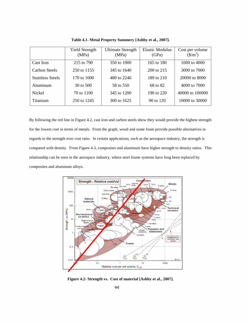
44
Table 4.1- Metal Property Summery [Ashby et al., 2007].
Yield Strength
(MPa)
Ultimate Strength
(MPa)
Elastic Modulus
(GPa)
Cost per volume
($/m3)
Cast Iron 215 to 790 350 to 1000 165 to 180 1000 to 4000
Carbon Steels 250 to 1155 345 to 1640 200 to 215 3000 to 7000
Stainless Steels 170 to 1000 480 to 2240 189 to 210 20000 to 8000
Aluminum 30 to 500 58 to 550 68 to 82 4000 to 7000
Nickel 70 to 1100 345 to 1200 190 to 220 40000 to 100000
Titanium 250 to 1245 300 to 1625 90 to 120 10000 to 30000
By following the red line in Figure 4.2, cast iron and carbon steels show they would provide the highest strength
for the lowest cost in terms of metals. From the graph, wood and some foam provide possible alternatives in
regards to the strength over cost ratio. In certain applications, such as the aerospace industry, the strength is
compared with density. From Figure 4.3, composites and aluminum have higher strength to density ratios. This
relationship can be seen in the aerospace industry, where steel frame systems have long been replaced by
composites and aluminum alloys.
Figure 4.2- Strength vs. Cost of material [Ashby et al., 2007].

45
Figure 4.3- Strength vs. Density [Ashby et al., 2007].
Durability for modular road plate applications can be evaluated by the wear and fatigue limits. Wear can be
defined by the following:
(4.1)
where:
ka = a measurement for the propensity of a sliding couple for wear ((MPa)-1
)
w = volume of material removed from contact surface / distance slid (m3)
Fn = applied bearing pressure * nominal area (N)
The constant ka is used to calculate the wear of the material over a certain force. Figure 4.4 helps identify
an inexpensive material as a wear surface for vehicles. A higher ka number represents a higher rate of wear.
From the Figure 4.4, steels have higher wear rates than some materials, such as, aluminum and copper.
However, for road application, proper limits of the forces need to be understood. This figure is created for wear
analysis of bearings where there are high repetitious forces. Therefore, a higher wear rate may still be

46
applicable. For example, a ball bearing would require a lower wear rate than a steel girder under pedestrian
loads.
Figure 4.4- Wear-rate Constant vs. Hardness [Ashby et al., 2007].
Considering the second part of durability, instead of the fatigue limit, the endurance limit can be used. The
endurance limit is the stress in the material where no fatigue failure will occur. The panels need to be designed
for either a finite or infinite fatigue life. The finite and infinite life boundaries lie between 106 and 10
7 cycles
for steels. A standard 5 axles truck would require 200,000 passes to reach the infinite life boundary; this would
take approximately 6 years if the traffic consists of 100 daily truck loads.
4.1.3 Polymers
Polymers are long chained structures composed mostly of carbon atoms. They have lower densities than
most metals, and have Young’s moduli that are lower than metals. Their strength to density ratio is similar to
that of metals. Polymers are easier to manufacture compared to metals because of their malleability and low

47
heat requirement. Polymers are separated into the following two categories: thermoset and thermoplastics.
Thermosets are polymers that can be heated only once. They are generally used for bonding agents of different
materials, such as fibreglass. Thermoplastics are polymers that can be reheated after they have set.
Elastomers can either be thermoplastics or thermosets, but have a lower Young’s modulus. They have low
elastic modulus because their polymer chain acts similar to springs. Rubbers are sometimes classified as
elastomers.
Table 4.2- Property Summery for Polymers [Ashby et al., 2007].
Yield Strength
(MPa)
Ultimate
Strength
(MPa)
Elastic Modulus
(GPa)
Cost per
volume ($/m3)
Polycarbonate 59 to 70 60 to 72 2 to 2.44 3000 to 4500
Polyethylene 18 to 29 21 to 45 0.621 to 0.896 1500 to 1750
Polypropylene 21 to 37 27 to 41 0.896 to 1.55 800 to 1250
Polystyrene 29 to 56 36 to 57 2.28 to 3.34 1500 to 2000
PVC 35 to 52 41 to 65 2.14 to 4.14 1250 to 2000
Polyurethane Elastomers 25 to 51 25 to 51 0.002 to 0.003 4000 to 9000
Natural Rubber 20 to 30 22 to 32 0.0015 to 0.0025 900 to 1100
Polymers are used heavily in temporary roadways because the material and construction costs are minimal.
In the report by Webster and Tingle [Webster and Tingle, 1998], plastic performed the worst out of all of the
material types. This may be due to the poor creep properties of plastics, even at room temperatures. The creep
temperature of polymers is 1/3 of the melting temperature (in Celsius) [Ashby et al., 2007]. In Webster and
Tingle’s study, the standard dimensions for metal and plastic sheet products are similar. Because of the
similarity in dimension and dissimilarity in strength, the polymer products are more likely to experience
structural failures than the corresponding metal products.
Lower melting temperatures make polymers easier to shape and manufacture than metals. Because of the
lower elastic modulus than metals, parts made with polymers can be easily fitted together. These advantages
combined with lower cost of dies and moulds would make polymers an affordable material from a
constructability standpoint.

48
4.1.4 Fibre-Reinforced Polymers
Fibre-reinforced polymers (FRPS) are hybrid materials. They combine the positive attributes of one
material, and offset its weaknesses with another material. The following are three main types of fibres that are
found in FRPs: glass reinforced polymer (GFPR), carbon reinforced polymer (CFRP), and Kevlar
(ARAMID).These reinforced polymers can be expensive to manufacture because of the complexity of the
hybridization. From Table 4.3, although the reinforced polymers have higher yield strengths than most metals,
the manufacturing cost is higher than that of most materials [Ashby et al., 2007].
Table 4.3- Strength, Elastic Modulus, and Cost for typical Fibre-Reinforced Polymers [Ashby et al.,
2007].
Yield Strength
(MPa)
Ultimate Strength
(MPa)
Elastic Modulus
(GPa)
Cost per volume
($/m3)
CFRP 550 to 1050 550 to 1050 69 to 150 70000 to 150000
GFPR 110 to 192 138 to 241 15 to 28 15000 to 40000
Kevlar 1000 to 1300 2600 to 2800 60 to 120 700000 to 750000
4.1.5 Wood
Wood is a natural material. Wood behaves similarly to unidirectional composite material due to the grain
direction. When the grains are in the direction of the load, the material can handle more stress. In terms of
specify strength (σf/ρ), wood and steel is similar. This may be one of the reasons that some manufactures still
use wood in matting products. Some of the typical wood properties are listed in Table 4.4. The typical wood is
matured wood of different species that are used for building structures. One of the disadvantages of using
wood is the non-uniformity of this material. For example, if a panel of wood contains a knot, it would severely
decrease the uniformity of stresses through the panel. Some existing products use hardwoods such as oak or
softwoods such as white fir [Eventsystems, 2011].
Table 4.4- Yield Strength, Ultimate Strength, and Elastic Modulus of Wood [Ashby et al., 2007].
Yield Strength
(MPa)
Ultimate Strength
(MPa)
Elastic Modulus
(GPa)
Wood Typical (longitudinal) 30 to 70 60 to 100 6 to 30
Wood Typical (transverse) 2 to 6 4 to 9 0.5 to 3
49
4.2 Modular Road System Design Concepts
In this section, the following four design concepts are described:
a simple plate design,
a sandwich panel design,
an asphalt tray design, and
a railway-inspired design.
4.2.1 Simple Plate Design
The first design considered for this study was a simple plate design. This design would consist of solid
panels, fabricated using one homogenous material. To select appropriate materials, constraint types are
required. These can be cost, weight, or strength. From the Figure 4.5, carbon steels and wood are shown to
have similar costs and strength ratios. These materials would therefore be good choices for use in a simple plate
system. When dealing with higher cost-to-strength ratios, the physical dimensions must be optimized to
minimized cost. Chapter 2 discusses this issue in more detail, where panels that are made of polymers and
composites are more complex in shape than wood and steel panels.

50
Figure 4.5- Comparing Cost and Strength with Different Materials.
Using a simple panel system, as shown in Figure 4.6, allows focus into other aspects of design, such as
connections. There are many possible connection types that can be considered in engineered structures. From a
civil engineering perspective, there are limits in the types of connections used due to environmental effects that
can occur. Connections must be selected based on ease of installation, ability to operate with minimal
maintenance, ability to handle load, constructability, and reusability.

51
Figure 4.6- Simple Plate Design.
Ease of the installations at the site can be achieved by using a connection design that is only one-
dimensional. For example, a hinge would only require a pin from one side after the two objects are connected.
A two dimensional installation, such as a universal joint, requires a pin to be installed from two different axes.
The increased number in axes during installation will increase the time required for installation. Also, if the
panels are hinged instead of fixed, the panels can be transported as connected pieces. Therefore, this could
eliminate the need to connect the panels at the job site.
The ability to operate with minimal maintenance requires the connection to operate under different
environmental conditions, such as operating despite the presence of foreign materials between the connections.
Most hinge connections require minimal friction at the joint connection to operate optimally. With the
introduction of foreign material or the lack of lubricants between the joints, the system will not operate
according to its intended purpose and may seize. As mentioned earlier in the literature review, the C-Hinge was
created to limit seizing by increasing tolerances. Hinges fix translational movement and allow for rotational
movement between the two objects. However, if the tolerances are large, the hinge may allow minor
translational movement between the two objects. The hinge can seize due to the extra degree of restriction
within the moving part. Therefore, a hinge with fewer degrees of restriction would decrease the possibility of
seizing. Hodgson created a self-aligning hinge [Hodgson, 1999], which allows rotational movement, but

52
restricts lateral movements. Hodgson’s hinge would accommodate the warping of doors because of the extra
degree of freedom when compared to a conventional door hinge.
Constructability involves the ability to create inexpensive and simple construction of the panels. Hinge
elements are more complex because they account for movement of the joints. The complexity is introduced due
to the extra construction steps required. Hinges can be moulded, cast, or machined [Poli, 2001].
Reusability means that the road system can be used again in the future. A quick turnaround time is
preferable. A fixed welded system is not suitable because it results in damage of the system at installation and
removal. A fixed bolted system is preferable because the bolts can be easily removed and replaced. Users with
any fastener system should be cautious during removal because tightening the bolts during thermal expansion
and obstructing foreign particles may seize the fasteners. Bolts are a fraction of the cost of the panel.
Therefore, new bolts should be used each time the bolt is installed. If the bolt is seized in the nut, forced
removal of the bolt can damage the panels and risk the replacement of the panel. Bolts are preferred over
screws because screws are tightened within the panel material, while bolts are tightened with nuts. When the
threads of a nut are stripped, the nut can be replaced easily, however, if the threads in the hole of the panel are
stripped, the panel may need to be repair or replaced.
The difference between a hinged and fixed connection is the ability for the connection to transfer moments.
With a hinged connection, there will be less stress between the separate panels, but more stress in the soil. The
panels beside the loaded panels do not fully support the load and it will bear downward into the soil. Therefore,
if these connections are similar in thickness, the hinged connection requires the support of a strong soil base,
while fixed connections require the support of a strong panel material.
The size of the panels can impact the overall structure of the system. If the panels are perfectly rigid, a large
panel can distribute a load on the subgrade better than a smaller panel of the same rigidity. By distributing the
load, the subgrade will less likely fail under bearing capacity. The faulting failure can also be decreased
because the difference in instantaneous forces is also decreased. If the panels are perfectly flexible, no matter
what size the panels are, the system will conform to the load and subgrade. A large panel would be more costly

53
to manufacture for the same quantity. For example, a panel that has the dimensions of two metres by two
metres will be more expensive than four panels that are one metre by one metre, because of the larger tooling
necessary to create the larger panels.
The panels must provide adequate friction for braking. Rubber of the tire has a coefficient of friction of
about 1 to 4 on dry steel [Ashby et al., 2007]. However, as the steel becomes damp, the water will drastically
decrease its coefficient. To allow for proper drainage, groves or grades in the panels must be designed to allow
for water drainage.
In most pavement structures, only reaction from adjacent slabs and the frictional forces constraints the
surface course layers laterally. Because of the lightness of these panels, there may be a need for the panels to be
connected to the ground. The forces that can move the panels may be lateral, longitudinal, or vertical. Lateral
forces come from the vehicle making lateral movements such as lane switching or turning. Longitudinal forces
can arise from the braking forces. Vertical forces can occur from the uplift of a passing vehicle. The uplift
occurs from the difference in air pressure at the bottom of the vehicle and the normal air pressure. To control
the lateral and longitudinal forces, frictional forces or actual anchors can be used. The required frictional forces
must be equivalent to the frictional forces that can be generated by calculating the weight of the panels and the
friction coefficient of the panel to soil (Equation 4.2) [Ashby et al., 2007]. If the required frictional forces
exceed the limit, an anchor system may be necessary. A simple anchor system can be a number of spikes
connecting the panel to the soil. To account for the vertical forces, the weight of the panels should be
considered. If the weight of the panels cannot hold the vertical forces, a hook system may be needed to hold
down the panels.
(4.2)
where:
= Lateral force of friction parallel to the surface
= coefficient of friction
= normal force exerted by the object to the surface

54
4.2.2 Sandwich Panel Design
The sandwich panel design concept is a variation of the simple plate concept, wherein the plate is
fabricated of layers – each made from a different material – arranged in such a way that the material chosen for
each layer is optimal, given the various functions performed by the layer. With this system, the flexural
stiffness of the plate can be maximized, while the cost and/or weight of the panel is minimized, by using stiff
materials for the outer layers with an inexpensive and/or light middle layer. An example of this system is to use
steel surfaces with a foam core. By placing the steel at the surface of the panel, the area moment of inertia is
increased. However, the core will carry most of the shear stresses because it would have a bigger volume than
the surface material. The core material must have proper thickness and strength to deal with the shear loads. In
certain parts of Canada, the temperature difference can be up to 60oC between 20OC and -33
OC [Environment
Canada, 2010]. Therefore, the core and surface materials should have similar thermal expansion properties and
be bonded strongly to each other. Figure 4.7 shows an example of a sandwich panel design where various
materials are combined.
Figure 4.7- Sandwich Panel Design.
4.2.3 Asphalt Tray Design
The asphalt tray design consists of a steel “tray” filled with cured asphalt. This design concept was
developed recognizing the success of asphalt as a material for constructing permanent roads. Thought was given
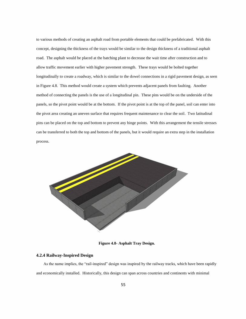
55
to various methods of creating an asphalt road from portable elements that could be prefabricated. With this
concept, designing the thickness of the trays would be similar to the design thickness of a traditional asphalt
road. The asphalt would be placed at the batching plant to decrease the wait time after construction and to
allow traffic movement earlier with higher pavement strength. These trays would be bolted together
longitudinally to create a roadway, which is similar to the dowel connections in a rigid pavement design, as seen
in Figure 4.8. This method would create a system which prevents adjacent panels from faulting. Another
method of connecting the panels is the use of a longitudinal pin. These pins would be on the underside of the
panels, so the pivot point would be at the bottom. If the pivot point is at the top of the panel, soil can enter into
the pivot area creating an uneven surface that requires frequent maintenance to clear the soil. Two latitudinal
pins can be placed on the top and bottom to prevent any hinge points. With this arrangement the tensile stresses
can be transferred to both the top and bottom of the panels, but it would require an extra step in the installation
process.
Figure 4.8- Asphalt Tray Design.
4.2.4 Railway-Inspired Design
As the name implies, the “rail-inspired” design was inspired by the railway tracks, which have been rapidly
and economically installed. Historically, this design can span across countries and continents with minimal

56
subgrade preparation. If it is assumed that the roads will support only a single lane of traffic, the vehicles
should not deviate from the lane unless there is an emergency or when the vehicle is driving off the road. Thus,
the main structural support is provided directly under the wheel lines. The rail-inspired system is similar to that
of the conventional rail system, except there is a platform that is placed on top of I-beams or “rails” on which
wheeled vehicles can drive. Under the rails are transverse wooden beams, similar to rail ties, which can be
replaced.
Temporary roadways constructed with lumber already exist (see Section 2.2). However, these roadways are
not sufficient for heavy vehicles and may fail under heavy loads [Manitoba Conservation and Water
Stewardship, 2012]. The purpose of the rails in the rail-inspired design is to distribute the load, so that the
lumber will be less likely to fail in flexure. The wooded beams distribute the rail loads more evenly to the soil,
thus preventing soil failures under heavy traffic loads. The design is shown in Figure 4.9.
Figure 4.9- Railway-Inspired Design.
4.3 Equivalent Plate Thickness Calculations
To obtain an approximate idea of the material quantities required for the simple plate system, an equivalent
plate thickness calculation was performed to determine the thickness of a plate constructed from a single,
homogenous material that would provide the same performance as a rigid concrete pavement. It is designed

57
according to the AASHTO Pavement Design Guide [American Association of State Highway and
Transportation Officials, 1993] for different soil conditions.
4.3.1 Calculation Methodology
Using the program StreetPave [American Concrete Pavement Association, 2011], rigid concrete pavement
designs based on the AASHTO Pavement Design Guide were obtained for a range of soil conditions. The
calculated thickness of the concrete pavement was then converted to an equivalent thickness for a simple plate
constructed from another material. Plate thicknesses providing an equivalent flexural strength, flexural
stiffness, and weight were thus established.
To calculate equivalent strength, the classic bending stress in a beam under simple bending is used (as
shown in equation 4.3) [Popov, 1991]. To determine the required thickness to withstand the same moment
while having the same surface footprint, the thickness and the material type can be varied. By rearranging the
bending stress equation, the relationship between material strength and thickness can be established. The
relation between appropriate material strength is the inverse square root of the thickness (Equation 4.4). For
example, if the material strength decreased by a factor of two then the thickness would require an increase of
four.
(4.3)
(4.4)
where:
= maximum stress of the beam
= moment supported in the beam (Nm)
= moment of inert (m4)
=height of the beam (m)
= perpendicular distance to the neutral axis (m)
= width of the beam (m)

58
This analysis should also be able to determine the equivalent thickness in terms of stiffness. Using the same
Euler-Bernoulli bending theory (Equation 4.4), the stiffness in terms of elastic modulus and curvature can be
isolated. While keeping the curvature, moments, and widths constants on right side of the equation, a
relationship between thickness and elastic modulus based on stiffness can be established. The material Young’s
Modulus is the inverse cube root of the thickness. For example, if the Young’s Modulus of the material is
decreased by a factor of two, then the thickness requirement would increase by a factor of eight.
(4.5)
where:
kbeam = resulting curvature of the beam
= Elastic modulus of the beam (MPa)
Finding equivalent thickness in terms of weight can be used to prevent movement of the pavement due to low
pressures of a passing vehicle. Given the standard definition of density (i.e. mass per unit volume), the
equivalent thickness can be calculated.
(4.6)
where:
w = mass (kg)
= density (kg/m3)
l = length (m)
w = width (m)
h = height (m)
Table 4.5 shows the summary of the equivalent thicknesses for strength, stiffness, and weight.

59
Table 4.5- Equivalent Thickness Equations for Calculation.
Equivalent Strength Thickness
4.3.2 Equivalent Stiffness Thickness
4.3.3 Equivalent Weight Thickness
4.3.4 Assumed Input Parameters
In order to perform the StreetPave analysis, the following input parameters in Table 4.6 were assumed.
Table 4.6- Input parameters for StreetPave Analysis.
Variable SI Unit Comment
Average Daily Truck Traffic 50 truck
vehicles
for high volume residential road [American
Concrete Pavement Association, 2011]
Modulus of Subgrade Reaction, k 1 MPa for typical silts and clays [Gunaratne, 2006]
Average 28-day Concrete Flexural
Strength
4.136
MPa
Concrete Modulus of Elasticity 27.5 GPa
Table 4.7 shows the list of materials that may be appropriate to be analysed for equivalent thickness.
Their strength, elastic modulus and density are required to calculate equivalent thicknesses.

60
Table 4.7- Strength, Stiffness, and Density Properties of Investigated Materials [Ashby et al., 2007].
Flexural Strength
(MPa)
Elasticity Modulus
(GPa)
Density
(g/cm3)
Al Alloy 200 200 2.70
Stainless Steel 500 200 7.85
High Carbon Steel 1000 100 7.85
Low Carbon Steel 500 150 7.70
HDPE 25.0 1.00 0.60
Polypropylene 100 4.00 1.20
Polycarbonate 80.0 5.00 1.40
ABS 65.0 4.00 1.10
CFRP 700.00 100.00 2.00
GFRP 150.00 20.00 1.69
Wood 60.00 20.00 1.64
Concrete 30.0 24.6 2.40
4.3.5 Calculation Results
With the equations in Table 4.5 and material properties listed in Table 4.7, the calculated rigid pavement
thickness was calculated for each material. The calculated equivalent thicknesses for the different materials are
summarized in Figure 4.10. Steel (stainless or carbon) appears to have the lowest equivalent thickness in terms
of strength, stiffness, and weight.

61
Figure 4.10- Equivalent Stress Thicknesses for Different Materials (k = 1 GPa).
For the majority of the cases in Figure 4.10, the stiffness is the limit for this design. This limit is similar to
the ridability criteria of conventional pavement, where the serviceability limit state is analyzed. The majority of
the failures that occur on conventional pavement are caused by the failure of material. (Section 3.5) It may be
appropriate to focus on the strength limit of the thickness with this design process. Therefore, the required
thickness for polymer or fibreglass can be decreased. This highlights the shortcomings of the empirical design
such that it cannot be used to design road plates for other materials, such as polymers and metals. To further the
analysis, finite element analysis should be used to calculate the interaction of the plate and soil.
4.3.6 Other Trial Thickness Considerations
There are a few places where materials other than asphalt and concrete are used in roadway construction
and can be examined to gain insight on the design requirements for a modular road plate system. Manhole
covers [Melnick and Melnick, 1994] are removable plates designed support vehicles passing over manholes.
They are able to distribute vehicle loads without yielding or crushing the supporting concrete. ASTM
[American Society for Testing and Material, 2007] specifies manhole covers of two different types and three
0
50
100
150
200
250
300
350
400 C
alcu
late
d T
hic
kne
ss (
mm
)
Strength
Stiffness
Weight
Concrete: Typical
Metals Polymers Fibreglass Metals Polymers Fibreglass

62
different grades. The different grades correspond with the thicknesses of the plate ranging from 6.5 mm to 12.5
mm. They have a top dimension of 381 mm by 584 mm or 457 mm by 610 mm.
4.4 Summary of Key Findings
Section 4.1 outlines many practical materials that can be used in the modular roadway system. There are
many unconventional materials that can be used with similar physical properties as asphalt and concrete, like
metals, plastics and fibre-reinforced. Section 4.2 showcases some creative methods in creating modular
roadways with current practices. These include pre-cured asphalt and railway like roadways. Section 4.3
highlights the different design limits and calculates appropriate initial panel thicknesses. There is currently no
process to design roadway with material other than concrete or asphalt.

63
Chapter 5
Finite Element (FE) Model and Study Descriptions
This chapter describes the finite element (FE) models developed to analyze modular road plate panels and
systems, along with the analytical studies performed using the developed models. A 2D single wheel (2D-SW)
FE model is described in Section 5.1, a 2D multiple wheel (2D-MW) FE model is described in Section 5.2, and
a 3D single wheel (3D-SW) FE model is described in Section 5.3. In Section 5.4, a number of barriers
encountered in the FE modelling are discussed, and in Section 5.5, the analytical studies performed with the
various FE models described in the preceding sections are described.
The computer program ABAQUS [Simulia, 2007] was used for the FE analysis presented in this thesis. In
order to ensure reasonable analysis times, the soil was modelled as a linear elastic material in all of the
presented FE analysis work. This is considered good practice in the early product design phase by a number of
researchers [Beskou, 2011, Helwany, 2007, Kim and Tutumluer, 2008, Wang, 2010]. In the analytical studies,
different scenarios are considered to cover a range of soil conditions, panel thicknesses, loading patterns, and
connection types. The analysis focused on the simple steel plate design, assuming that the same methodology
can be extended to other plate systems and materials in the future.
5.1 2D Single Wheel (2D-SW) FE Model
Prior to performing the analytical studies, the assumed model boundary conditions and level of mesh
refinement are needed to be validated. In order to do this, a 2D single wheel (2D-SW) FE model was
employed. The main parameters investigated were the volume of soil under a single road plate that needed to
be modelled for accurately simulating a semi-infinite volume of soil below the plate, and the level of mesh
refinement needed to accurately predict the stresses in the steel plate and soil under a design wheel load. In
order to perform this validation step efficiently, a 2D FE model was employed.
5.1.1.1 2D-SW Model Description
The 2D single wheel (single plate) models (2D-SW) were created to determine the appropriate boundaries
for the FE analysis. Figure 5.1 defines the critical dimensions of the 2D model. If the wheel load is applied at

64
the centre of the road plate, then the symmetry of the problem can be exploited to cut the required number of
elements in half, as illustrated in Figure 5.1. The confining effects of the soil adjacent to the bottom and left
hand sides of the soil volume are modelled by restraining displacements along these edges in a direction
perpendicular to the edge. The soil volume in this figure is determined by the “modelled width” and “depth”
dimensions. A 1 m x 1 m square plate is assumed, with a thickness that can vary. The wheel load modelled
was the heaviest wheel load in the CAN/CSA-S6 CL-625-ONT design truck [Canadian Standards Association,
2006]. The heaviest, fourth axle wheel load is modelled. This wheel introduces a load of 87.5 kN over a 0.6 m
x 0.25 m area. This load is modelled by applying a uniform pressure of 0.5833 MPa over the loading area. This
loading corresponds to the unfactored wheel load for this design truck and does not consider dynamic effects,
which are normally considered in bridge design using a dynamic load allowance (DLA) factor.
Figure 5.1- 2D single wheel (2D-SW) model.

65
Table 5.1 shows the ranges and increments considered for the variable parameters in the boundary
condition and mesh refinement validation study. These parameters included the modelled width and width, and
the mesh size. In order to confirm the influence of the plate thickness and soil stiffness on the results, these
parameters were also varied. Resilient Modulus (MR) is an estimate of the modulus of elasticity of the soil.
However, in ABAQUS, an elastic modulus must be prescribed. There are correlations between California
Bearing Ratio (CBR) and MR [American Association of State Highway and Transportation Officials, 1993] as
stated in Equation 5.1.
(5.1)
Table 5.1- Variables in 2D single wheel (2D-SW) validation study.
Variables Range Increments
Width 0 - 1000 cm 0, 50, 100, 250, 500, 750, 1000
Depth 1 - 50 m 1, 5, 10, 25, 50
Mesh 1 -500 mm square mesh 1, 5, 10, 50, 100, 250, 500
Thickness 1 - 20 mm 1, 20 mm
Resilient Modulus 1 – 50 MPa 1, 50 MPa
The panel and base have an interaction property of frictionless and hard surface with adjustment for over
closures. Different surface contacts were tested within the Abaqus program to determine which would derive
possible results. Contact errors are one of the main concerns with building the model because the models
should not only give a probable solution, but also an actual solution. For example, if the contacts were not
properly constrained, the models would not find a solution due to convergence issues. While modeling, the
convergence issues occur during improper constraints of the items in the model and the contacts between the
items. When the contacts are not tied down nor have proper friction properties, the dynamic instability would
occur in the model where the panels will attempt to slide out of the soil. However, Abaqus has difficulties
modeling friction between two surfaces because of the discontinuity between sticking and slipping [Simulia,
2007]. This can cause convergence issues especially in small increments. The models require small increments

66
to solve large deformations because of the elastic difference in the two materials, namely soil and panel. To
eliminate the dynamic instability, the middle of the panel is tied down to the soil. A hard surface with
adjustment for over closures was used to ensure that the nodes for the two different parts would not penetrate
each other within the contact area.
In practice, plane strain should be used for very thick continuum while plane stress should be used for very
thin continuum. In this analysis, the soil is relatively thick while the panels are relatively thin. The soil element
uses the family of plane strain elements because the strain that is out of the plane is relatively small compared to
the other strains. Similar analyses are used for dams where the object’s length is greater than the in-plane
dimensions. The panel uses a beam element specified by Abaqus because the panel object uses a line element
and not a shell element. Using the beam element format allows the line to show a beam cross-section and the
associated rigidity. It would be difficult to obtain an accurate solution with the panel if the shell elements are
used in a 2D format due to the large differences between the thickness and the length. The node distance of
panels are 25 mm apart, while the node distance of the soil is 50 mm apart. These numbers were chosen
because the nodes of the two objects must line up. These node densities allow for a 95% accuracy of the model.
Both objects used a linear geometric order because the simplicity of the model was sufficient for this analysis.
By analyzing the model in two dimensions, the results will be similar to a strip foundation where the out of
plane is infinitely long when compared to the in plane dimensions. This would not be an accurate
representation of the actual model proposed because the load patch is 0.6 m by 0.25 m and the panel size is 1 m
by 1 m. The two dimensional model may give a higher stress and deformation value because the loads are not
distributed out of plane. Although this model may not provide an accurate depiction of the actual model, it can
show how different panel sizes affect the stresses and deformations.
Using a two dimensional model, modeling a 0.6 m of load has a similar effect of modeling a continuous
depth of the model. This creates a model similar to a continuous spread footing or strip footing. This
simplification may lead to stresses which are larger than the actual because the actual load is a small patch load
rather than a continuous strip load. The element type used for the panel is a line element while the soil uses a
shell element. The shell element was used as advised by the Abaqus Manual [Simulia, 2007] and Robinson

67
[Robinson et al., 2011] because the panel thicknesses are significantly smaller than other dimensions in the
structure.
In order to examine convergence as the mesh was refined and the soil volume increased, the following
parameters were monitored: 1) the maximum stress in the panel, 2) the maximum deformation, and 3) the
maximum stress in the soil. The Von Mises stress was compared because it analyses both the shear and the
principle stress to create a more accurate range for failure.
In Chapter 6, the results of this validation study are presented for the following cases: 1) the weakest soil
subgrade modulus (1 MPa) with the minimum panel thickness (1 mm), and 2) the strongest soil resilient
modulus (50 MPa) with the maximum panel thickness (20 mm).
5.2 Multi-Wheel (2D-MW) Model
Following the 2D-SW validation studies, a 2D multi-wheel (2D-MW) model was developed to investigate
how the multi-wheel truck load would impact a multi-panel system. In the single wheel model, only the wheel
load associated with the heaviest fourth axle was considered. However, because the second and third axial are
close together, it was speculated that this axle group might be critical for multi-panel system design. In the
CAN/CSA-S6 bridge code [Canadian Standards Association, 2006], the combination of the second and third
axles, and the individual fourth axle may be critical depending on the length of the bridge component that is
being designed. In the 2D-MW model, a continuous panel is stretched over the outside-to-outside distance
between the first and last wheel load patches plus 0.375 m on either side of the truck to not let the load be at the
edge of the panel. An edge loaded panel creates eccentric load, which would induce larger stresses in the soil
than a panel loaded principally. In doing this, a moment resisting connection is effectively being assumed
between panels. The height (2.0 m), modelled width (0.5 m), and mesh size (1 cm) for the multi-wheel model
were chosen based on the results of the 2D single wheel analysis. Figure 5.2 shows how the loads and the shape
dimension. The 2D-MW model was similar to the 2D-SW model in most other respects, except that symmetry
was not assumed in the 2D-MW model because the axle configuration of the design truck is not symmetrical.
The different items in the models were horizontally constrained. The soil was constrained at the bottom surface

68
while the panels were tied into the top of the soil surface at the middle of the maximum pressure load, which is
the fourth axle. The multi-wheel model was used to examine the following two different cases: 1) the softest
soil resilient modulus (1 MPa) with the minimum panel thickness (1 mm), and 2) the stiffest soil resilient
modulus (50 MPa) with the maximum panel thickness (20 mm). Similar to the 2D-SW model in Chapter 6 , the
Von Mises panel stress, deformation, and soil stress are compared for these two cases.
Figure 5.2- 2D multi-wheel (2D-MW) model (all dimensions in metres).
5.3 3D Single Wheel (3D-SW) Model
In order to investigate possible concerns surrounding the simplifying assumptions required to implement
the 2D models, a 3D single wheel (3D-SW) model was subsequently developed. This is more accurately
simulated with out-of-plane stresses and strains in the system. For the 3D-SW studies, the panel dimensions in
plan were held constant at 1 m x 1 m. The soil volume was modelled with a depth of 1.0 m and an modelled
width of 0.5 m on all four sides of the panel. Symmetry was not assumed, since one of the goals of the 3D-SW
analysis was to model the effects of eccentrically loading the plate.
In order to study the effects of the panel connection type, the following two versions of the 3D-SW model
were developed: one is to model a single panel and the other is to model a four panel “system”. In both cases,
single wheel loading was modelled. In the four panel model, the total plane area of the four panels was 2 m x 2
m and the depth and modelled width of the soil volume was the same as in the single panel model.
Axle 4 Wheel Load
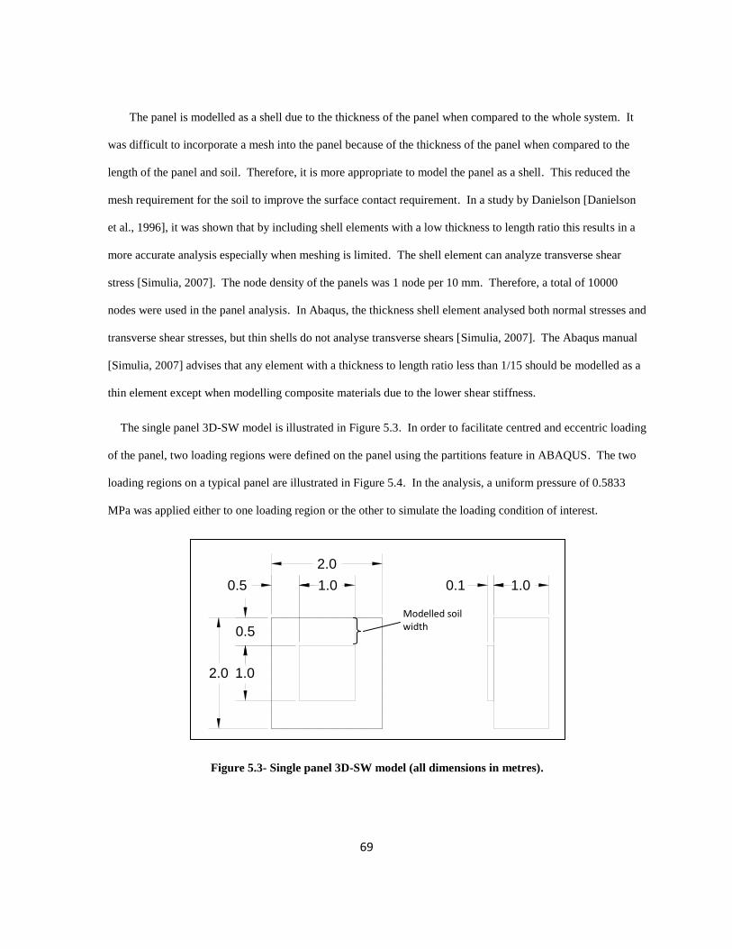
69
The panel is modelled as a shell due to the thickness of the panel when compared to the whole system. It
was difficult to incorporate a mesh into the panel because of the thickness of the panel when compared to the
length of the panel and soil. Therefore, it is more appropriate to model the panel as a shell. This reduced the
mesh requirement for the soil to improve the surface contact requirement. In a study by Danielson [Danielson
et al., 1996], it was shown that by including shell elements with a low thickness to length ratio this results in a
more accurate analysis especially when meshing is limited. The shell element can analyze transverse shear
stress [Simulia, 2007]. The node density of the panels was 1 node per 10 mm. Therefore, a total of 10000
nodes were used in the panel analysis. In Abaqus, the thickness shell element analysed both normal stresses and
transverse shear stresses, but thin shells do not analyse transverse shears [Simulia, 2007]. The Abaqus manual
[Simulia, 2007] advises that any element with a thickness to length ratio less than 1/15 should be modelled as a
thin element except when modelling composite materials due to the lower shear stiffness.
The single panel 3D-SW model is illustrated in Figure 5.3. In order to facilitate centred and eccentric loading
of the panel, two loading regions were defined on the panel using the partitions feature in ABAQUS. The two
loading regions on a typical panel are illustrated in Figure 5.4. In the analysis, a uniform pressure of 0.5833
MPa was applied either to one loading region or the other to simulate the loading condition of interest.
Figure 5.3- Single panel 3D-SW model (all dimensions in metres).
2.0
2.0
0.5 1.0
0.5
1.0
1.00.1
Modelled soil width

70
Figure 5.4- Panel loading locations (all dimensions in metres).
The four panel 3D-SW model, illustrated in Figure 5.5, consists of four panels placed together in a square
formation. The load is placed on Panel 1 in the inner corner as an eccentric load to simulate centre loading on
the four panel system. This approach was used to allow direct comparison with the eccentrically loaded single
panel analysis. The following two connection types were assumed in the four panel analysis: 1) fixed or
“moment” connections which link displacements and rotations along connected panel edges, and 2) pinned or
“hinged” connections which link the displacements but allow rotations to differ at the edges of the connected
panels. Continuous connections were assumed along the entire length of each connected panel edge.
Center Loading
Eccentric Loading0.6
0.3
0.1
0.3
0.2 0.6
0.25
0.25

71
Figure 5.5- Four panel 3D-SW model (all dimensions in metres).
In the single panel 3D-SW analysis, the panels were tested with two different types of loading: centred and
eccentric. The centre loading was determined as the best case scenario because the load is evenly distributed
over the panel area. The eccentric loading was thought to represent a worst case scenario because less area of
the panel participated in distributing the load.
In the four panel 3D-SW analysis, only one loading configuration was considered. However, the following
two connection types were analyzed: hinged and fixed. The purpose of these panel analyses was to determine
how the connection type affects the extent to which the adjacent panels contribute to redistributing the load in a
multi-panel modular road plate system.
5.4 Modeling Difficulties
A number of convergence issues were encountered in the 3D-SW models due to the large deflections
involved, and the large differences between the elastic moduli of the soil and the panel materials. During the
eccentric loading analysis, the convergence issues were generally more prevalent.
Constraints were added to prevent the panel from misalignment with the eccentric load, as suggested in
[Sun and Sacks, 2005] to help solve convergence issues. This study was used because it attempts to analyse
biomechanical material interacting with soft tissues, which is similar to this thesis such that a hard material (the
panel) interacts with a soft material (the soil). In the 3D-SW analysis, a point in the middle of the loading patch
0.5
1.0
1.0
3.0
0.5 1.0 1.0 0.1 2.0
3.0
1 2
3 4
Loading
Modelled soil width

72
was selected to be constrained in the in-plane rotational and horizontal translational axes. Without this
constraint, the model would experience convergence issues because the panels would not be statically stable.
In all the analyses, the modelling steps were decreased to introduce the load more gradually, as suggested in
[Zienkiewicz et al., 2005]. With the proper initial rate of loading, the panels are able to align with the soil and
limit the over-closure and mesh rippling. Because of the difference between the moduli of the panel and the soil
material, the lower step sizes were required.
5.5 Analytical Study Description
Section 5.3 summarizes all of the analyses performed using the 3D-SW single and four panel models.
Seven panel thicknesses and seven soil stiffness were modelled, resulting in 49 analyses per panel
configuration. The following four panel configurations were analyzed: single panel with centre loading
(1CNU), single panel with eccentric loading (1ENU), four panels with fixed connections (4ENF), and four
panels with pinned connections (4ENP). These resulted in a total of 196 analyses performed.
Table 5.2- Summary of FE analyses performed.
Variables Range Scenarios
Panel thickness 1 mm to 20 mm 1, 2, 3, 5, 10, 15, 20 MPa (7 cases)
Resilient Soil
Modulus
1 MPa to 50
MPa 1, 5, 10 , 20, 30, 40, 50 MPa (7 cases)
number of panels 1 to 4 1 panel, 4 panels
connection type hinged and fixed
5.6 Summary of Input Design Values
Table 5.3 summarizes the investigated input ranges for model calculation as suggested in the previous
sections. These values are used during the analysis in the next chapter.

73
Table 5.3- List of Input Variables with Corresponding Values.
Input Variable Value Constant Comment
Traffic 87.5 kN or 0.583 MPa Yes See 3.1.1
Subgrade Modulus 1 - 50 MPa No See 3.5.1
Young’s Modulus of Steel 200 GPa Yes 5.6.1 [Ashby et al., 2007]
Table 5.4- List of Failure Criteria with Corresponding Values.
Failure Criteria Value Comment
Steel Yield Strength 350 MPa [Ashby et al., 2007]
Deformation Limit 20 mm
Table 3.3.
Table 3.3
Soil Bearing Capacity Soil Dependent
Table 3.1
5.7 Summary of Key Findings
Chapter 5 summarized to build the model correctly in order obtain proper data. The 2D single wheel model
(in Section 5.1) studied the sensitivity of the physical shape of the model. The 2D multi wheel model (in
Section 5.2) studied how different load patterns can create larger loads. The 3D model (in Section 5.3) shows
the final models which will general the FEM. Section 5.4 describes modelling difficulties, such as convergence
and contact issues. These were solved by having smaller incremental time, preloading the models, and proper
model contacts.

74
Chapter 6
FE Analysis Results
In this chapter, the results of the various finite element (FE) analysis studies described in Chapter 5 are
presented. In Sections 6.1-6.3, the FE analysis results obtained using the 2D single wheel (2D-SW), 2D multi-
wheel (2D-MW), and 3D single wheel (3D-SW) models respectively are presented. In Section 6.4, area graphs
are developed based on the 3D-SW FE analysis results, for the rapid design of modular road systems consisting
of 1 m x 1 m steel plates under a wide range of soil conditions.
6.1 Single Wheel (2D-SW) FE Model Results
Figure 6.1 shows the typical deformed shape of the soil below a centre loaded steel road panel, according to
the 2D-SW analysis. In Figure 6.1, the road plate deformation is also visible. In particular, the uplift of the
plate at its outer edge can be seen. This uplift occurred in only some cases because with a rigid panel the panel
does not flex upward.
Figure 6.1- Typical deformed shape from 2D-SW analysis (Esoil=10 MPa and tpanel = 20 mm).
The 2D single wheel (2D-SW) analysis was used to determine the mesh refinement, and the modelled soil
depth and width to be used in the 2D-MW and 3D-SW analyses. The results of these analyses are summarized
in Figures 6.2-6.4. In these figures, the stress and deformations are divided by the maximum value in the series,
since the main objective of these analyses was to determine when the results stabilize as the level of mesh
refinement, or the modelled soil depth or width are increased. The data series are categorized to a panel stress
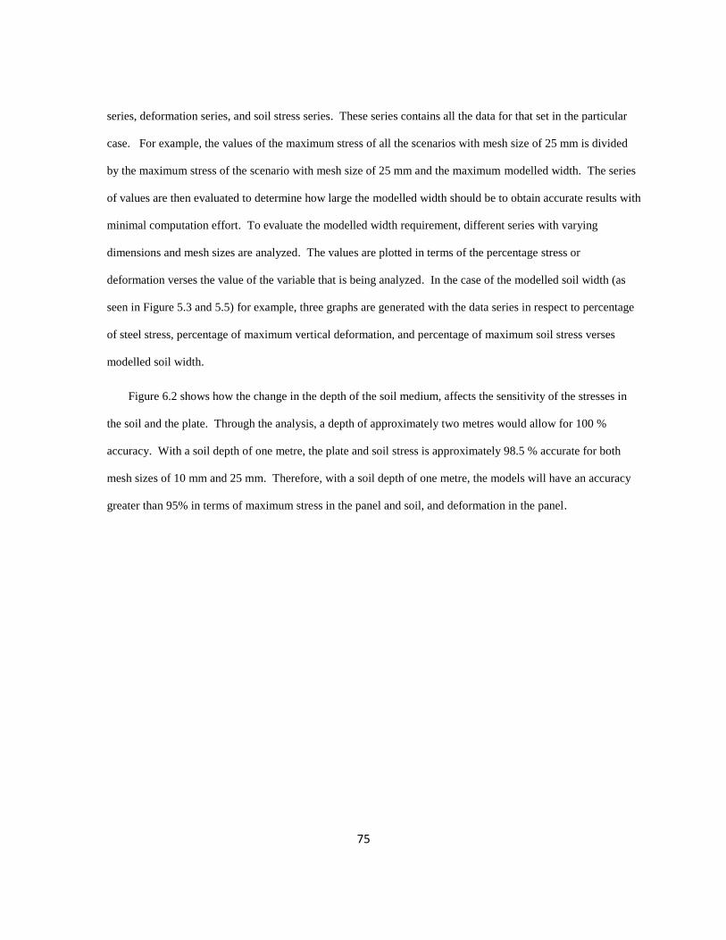
75
series, deformation series, and soil stress series. These series contains all the data for that set in the particular
case. For example, the values of the maximum stress of all the scenarios with mesh size of 25 mm is divided
by the maximum stress of the scenario with mesh size of 25 mm and the maximum modelled width. The series
of values are then evaluated to determine how large the modelled width should be to obtain accurate results with
minimal computation effort. To evaluate the modelled width requirement, different series with varying
dimensions and mesh sizes are analyzed. The values are plotted in terms of the percentage stress or
deformation verses the value of the variable that is being analyzed. In the case of the modelled soil width (as
seen in Figure 5.3 and 5.5) for example, three graphs are generated with the data series in respect to percentage
of steel stress, percentage of maximum vertical deformation, and percentage of maximum soil stress verses
modelled soil width.
Figure 6.2 shows how the change in the depth of the soil medium, affects the sensitivity of the stresses in
the soil and the plate. Through the analysis, a depth of approximately two metres would allow for 100 %
accuracy. With a soil depth of one metre, the plate and soil stress is approximately 98.5 % accurate for both
mesh sizes of 10 mm and 25 mm. Therefore, with a soil depth of one metre, the models will have an accuracy
greater than 95% in terms of maximum stress in the panel and soil, and deformation in the panel.

76
Figure 6.2- Effect of soil depth on plate stress, deformation, and soil stress for the weakest soil.
Figure 6.3 shows how the modelled soil width affects the sensitivity of the model by comparing stresses
and strains. As the modelled soil width increases, the stresses and deformation will appear explicit. If the
modelled soil width extends at least one metre past the panel edge, the model appears to result in 95 %
accuracy.
2000 4000 6000 8000 100000.94
0.96
0.98
1
Height of Soil (mm)
Pla
te S
tre
ss P
rece
nta
ge
(%
)
Plate Stress - Depth Analysis
2000 4000 6000 8000 100000.94
0.96
0.98
1
Height of Soil (mm)
De
form
atio
n P
rece
nta
ge
(%)
Deformation - Depth Analysis
2000 4000 6000 8000 100000.94
0.96
0.98
1
Height of Soil (mm)
So
il S
tre
ss P
rece
nta
ge
(%)
Soil Stress - Depth Analysis
Mesh size of 10 mm
Mesh size of 25 mm
95% Limit

77
Figure 6.3- Effect of modelled soil width on plate stress, deformation, and soil stress.
Figure 6.4 shows how the mesh size affects the sensitivity of the model by comparing different stresses and
strains. As the mesh size increases, the accuracy of the model decreases. When a mesh size of 50 mm was
used, an accuracy of 97 % was recorded.
102
103
104
0.94
0.96
0.98
1
Extended Edge Distance (mm)
Pla
te S
tre
ss P
rece
nta
ge
(%
)Plate Stress - Extension Analysis
102
103
104
0.94
0.96
0.98
1
Extended Edge Distance (mm)
De
form
atio
n P
rece
nta
ge
(%
)
Deformation - Extension Analysis
102
103
104
0.94
0.96
0.98
1
Extended Edge Distance (mm)
So
il S
tre
ss P
rece
nta
ge
(%
)
Soil Stress - Extension Analysis
Mesh size of 10 mm
Mesh size of 25 mm
Mesh size of 50 mm
Mesh size of 100 mm
95% Limit

78
Figure 6.4-Effect of mesh size on plate stress, deformation, and soil stress.
For practical reasons, a convergence criterion of 95% accuracy was assumed for determining the acceptable
levels of mesh refinement, soil depth, and modelled soil width. During the analysis of the modelled soil width
in Figure 6.3, 95% accuracy was achieved with a modelled soil width of 500 mm. In the mesh refinement study
in Figure 6.4, a mesh size of 50 mm was required to achieve 95% accuracy. In the soil height study in Figure
6.2, a required height of 1-2 m was found to obtain 95% accuracy.
6.2 Multi-Wheel (2D-MW) FE Model Results
The purpose of the 2D multi-wheel (2D-MW) analysis was to study the effects of multi-wheel axle groups
acting simultaneously on a continuous multi-panel road plate system. Figure 6.5 shows a comparison of the
“strong” and “weak” scenarios defined in Chapter 5. The strong scenario consisted of a 20 mm thick panel
supporting the entire CAN/CSA S6-06 CL-625 truck model on a soil with a subgrade modulus of 50 MPa. The
weak scenario consisted of a 1 mm thick panel supporting the entire CL-625 truck on a soil with a subgrade
0 20 40 60 80 1000.94
0.96
0.98
1Plate Stress - Mesh Analysis
Mesh Size (mm)
Pla
te S
tre
ss P
rece
nta
ge
(%
)
0 20 40 60 80 1000.94
0.96
0.98
1Deformation - Mesh Analysis
Mesh Size (mm)
De
form
atio
n P
rece
nta
ge
(%
)
0 20 40 60 80 1000.94
0.96
0.98
1Soil Stress - Mesh Analysis
Mesh Size (mm)
So
il S
tre
ss P
rece
nta
ge
(%
)
Extended Soil Distance from Plate = 0 mm
Extended Soil Distance from Plate = 250 mm
Extended Soil Distance from Plate = 500 mm
Extended Soil Distance from Plate = 750 mm
Extended Soil Distance from Plate = 1000 mm
Extended Soil Distance from Plate = 5000 mm
Extended Soil Distance from Plate = 9000 mm
95% Limit

79
modulus of 1 MPa. Both scenarios did not include dynamic loading as previously mentioned. Figure 6.5 shows
the panel Von Mises stress, deformation, and soil Von Mises stress along the plate. Looking at this figure, the
rigid panel distributes stresses and strain more evenly than a flexible panel. Figure 6.6 shows the stress
distributions in the panel and the soil with the corresponding stress range legends in Figure 6.7 and Figure 6.8.
These figures show how the forces are distributed under the soil surface. The top number represents the axle
number of the truck. The second row of numbers represents the specific axle weight and the last row represents
the wheel loads. The wheel load pressure was used to model the loading in each individual location.
Figure 6.5- 2D-MW analysis results for strong and weak scenarios.
0 0.2 0.4 0.6 0.8 1 1.2 1.4 1.6 1.8 2
x 104
0
10
20
30
40
50
Pla
te S
tre
ss (
MP
a)
True Distance Along Path (mm)
Strong Scenario
Weak Scenario
0 0.2 0.4 0.6 0.8 1 1.2 1.4 1.6 1.8 2
x 104
-60
-40
-20
0
20
De
form
atio
n (
mm
)
True Distance Along Path (mm)
0 0.2 0.4 0.6 0.8 1 1.2 1.4 1.6 1.8 2
x 104
0
0.05
0.1
0.15
0.2
0.25
So
il S
tre
ss (
MP
a)
True Distance Along Path (mm)

80
Figure 6.6- Plate and soil stresses with wheel load pattern (weak scenario- all units are in kN).
Figure 6.7- Von Mises Stress Legend for Panel
Distribution.
Figure 6.8- Von Mises Stress Legend for Soil
Distribution.
6.3 Single Wheel (3D-SW) Model
With the knowledge gained from the 2D models, 3D single wheel (3D-SW) models were constructed and
analyzed to consider the 3D stress states in the panel and soil more accurately, and to study the effects of the
plate connection type and eccentric plate loading on the analytical results. The results of the 3D-SW analyses
are summarized in Figure 6.9 to 6.15. These results are compared in terms of the panel stress, deformation, and
soil stress verses modulus of subgrade of the soil. The thickness of the steel plate is the main design variable.
The panel stress results are compared with the nominal unfactored yield strength of the steel (350 MPa) to give
an indication of an acceptable minimum plate thickness. The soil stress results are compared with bearing stress
limits of soil having different shear angles. The deflection results are compared with deflection limits for
conventional concrete pavement. They are also compared to the ideal cases of a perfectly rigid panel and no
panel at all (i.e. tire acting directly on soil).

81
In the panel stress graphs, Von Mises stresses are plotted at the top left side of the results figure (Figure 6.9,
Figure 6.11, Figure 6.13, and Figure 6.14). In the deformation graph, the displacement limit and theoretical
values are compared with the data series. Limits set by Table 2.1 are shown in the graph as a different limiting
line. The foundation model deformation limit is calculated from Boussinesq’s equation as a plate load of 0.25
m by 0.60 m. The basic elastic deformation limit is calculated using Hooke’s Law, and the elastic modulus to
calculate the deformation is based on the vertical truck load. This limit assumes that the forces are fully
vertically distributed in the material. In the soil stress graphs, the soil stresses are soil bearing stresses (or
defined in Abaqus as contact pressure). These can be compared to the limiting stresses calculated using the
bearing capacity equation with different shear angles considered to model different soil types.
In Figure 6.9, the results are presented for the case of a single plate with the tire load centred (1CNU). An
image of the deformed shape and Von-Mises stress contours for this analysis case are presented in Figure 6.10.
Similar results are presented for the eccentric loading (1ENU) case in Figure 6.11 and Figure 6.12. Figure 6.13
and Figure 6.14 present the results for the analyses of the four panels fixed connection (4ENF) and four panel
pinned connection (4ENP) respectively. An image of the deformed shape for the latter case is presented in
Figure 6.15.
Figure 6.9 shows the results of a single panel loaded with a single tire load in the centre of the panel.
Maximum panel stress, soil stress, and vertical deformation increased when the steel thickness is decreased.
Increasing the soil elasticity decreases the panel stress and deformation; however, if the soil elasticity changes
without the panel thickness changing, the stress in the soil does not change drastically.

82
Figure 6.9- Single panel centre loading (1CNU) analysis results.
Figure 6.10 shows the deformation and stress of the single panel loaded with a single tire load in the centre
of the panel. The stresses are focus in the centre of the panel, where the wheel load occurred.
0 10 20 30 40 500
200
400
600
800
1000
12001CNU-Panel Data
Soil Elastic Modulus (MPa)
Pa
ne
l S
tre
ss M
Pa
)
Steel Yield Stress, Unfactored
0 10 20 30 40 500
100
200
300
4001CNU-Deformation Data
Soil Elastic Modulus (MPa)
Ve
rtic
al D
efo
rma
tio
n (
mm
)
Foundation Model H=2
Basic Elastic H=2
Severe Potholes
Very Severe Potholes
Severe Rutting 20mm
Very Severe Rutting 50mm
0 10 20 30 40 500
0.2
0.4
0.6
0.8
11CNU-Soil Data
Soil Elastic Modulus (MPa)
So
il S
tre
ss (
MP
a)
Rigid Panel on Soil
Wheel on Soil
Theta=35
Theta=36
Theta=37
Theta=38
Steel Thickness = 1 mm
Steel Thickness = 2 mm
Steel Thickness = 3 mm
Steel Thickness = 5 mm
Steel Thickness =10 mm
Steel Thickness =15 mm
Steel Thickness =20 mm
Concrete Thickness =120 mm
Concrete Thickness =130 mm
Concrete Thickness =140 mm
Concrete Thickness =150 mm
No Panel, Imprint of 0.6 m, 0.25 m
No Panel, Imprint of 1 m, 1 m

83
Figure 6.10- Deformed shape and Von-Mises stress contours for 1CNU analysis.
Figure 6.11 shows the results of a single panel loaded with a single tire load in the corner of the panel.
Similar to Figure 6.9, the panel stress increased as the panel thickness decrease. However, as the panel
thickness increase, the soil stresses also increase. The vertical deformation did not change when there was a
change in panel thickness.

84
Figure 6.11- Single panel eccentric loading (1ENU) analysis results.
Figure 6.12 shows the deformation and stress of the single panel loaded with a single tire load in the corner
of the panel. The stresses are focus in the top corner of the panel, where the wheel load occurred.
0 10 20 30 40 500
200
400
600
800
1000
12001ENU-Panel Data
Soil Elastic Modulus (MPa)
Pa
ne
l S
tre
ss M
Pa
)
Steel Yield Stress, Unfactored
0 10 20 30 40 500
100
200
300
4001ENU-Deformation Data
Soil Elastic Modulus (MPa)
Ve
rtic
al D
efo
rma
tio
n (
mm
)
Foundation Model H=2
Basic Elastic H=2
Severe Potholes
Very Severe Potholes
Severe Rutting 20mm
Very Severe Rutting 50mm
0 10 20 30 40 500
0.2
0.4
0.6
0.8
11ENU-Soil Data
Soil Elastic Modulus (MPa)
So
il S
tre
ss (
MP
a)
Rigid Panel on Soil
Wheel on Soil
Theta=35
Theta=36
Theta=37
Theta=38
Steel Thickness = 1 mm
Steel Thickness = 2 mm
Steel Thickness = 3 mm
Steel Thickness = 5 mm
Steel Thickness =10 mm
Steel Thickness =15 mm
Steel Thickness =20 mm
Concrete Thickness =120 mm
Concrete Thickness =130 mm
Concrete Thickness =140 mm
Concrete Thickness =150 mm
No Panel, Imprint of 0.6 m, 0.25 m
No Panel, Imprint of 1 m, 1 m

85
Figure 6.12- Deformed shape and Von-Mises stress contours for 1ENU analysis.
Figure 6.13 shows the results of four fix connected panel loaded with a single tire load in the centre of the
panel. The shapes of the graphs appear similar to Figure 6.9. Maximum panel stress, soil stress, and vertical
deformation increased when the steel thickness is decreased. Increasing the soil elasticity decreases the panel
stress and deformation. However, if the soil elasticity changes without the panel thickness changing, the stress
in the soil does not change drastically. The loading results are similar to that of a single panel loaded with a
single tire load in the centre of the panel.

86
Figure 6.13- Four panel fixed connection (4ENF) analysis results.
Figure 6.14 shows the results of four pin connected panel loaded with a single tire load in the centre of the
panel. The shapes of the graphs appear similar to Figure 6.11. Similar to Figure 6.13, the panel stress increased
as the panel thickness decrease. However, as the panel thickness increase, the soil stresses also increase. The
vertical deformation did not change when there was a change in panel thickness. The loading results are similar
to that of a single panel loaded with a single tire load in the corner of the panel.
0 10 20 30 40 500
200
400
600
800
1000
12004ENF-Panel Data
Soil Elastic Modulus (MPa)
Pa
ne
l S
tre
ss M
Pa
)
Steel Yield Stress, Unfactored
0 10 20 30 40 500
100
200
300
4004ENF-Deformation Data
Soil Elastic Modulus (MPa)
Ve
rtic
al D
efo
rma
tio
n (
mm
)
Foundation Model H=2
Basic Elastic H=2
Severe Potholes
Very Severe Potholes
Severe Rutting 20mm
Very Severe Rutting 50mm
0 10 20 30 40 500
0.2
0.4
0.6
0.8
14ENF-Soil Data
Soil Elastic Modulus (MPa)
So
il S
tre
ss (
MP
a)
Rigid Panel on Soil
Wheel on Soil
Theta=35
Theta=36
Theta=37
Theta=38
Steel Thickness = 1 mm
Steel Thickness = 2 mm
Steel Thickness = 3 mm
Steel Thickness = 5 mm
Steel Thickness =10 mm
Steel Thickness =15 mm
Steel Thickness =20 mm
Concrete Thickness =120 mm
Concrete Thickness =130 mm
Concrete Thickness =140 mm
Concrete Thickness =150 mm
No Panel, Imprint of 0.6 m, 0.25 m
No Panel, Imprint of 1 m, 1 m

87
Figure 6.14- Four panel pinned connection (4ENP) analysis results.
Figure 6.15 shows the deformation and stress of the four pin connected panel loaded with a single tire load
in the centre of the panel. The stresses are focus in the centre of the panel, where the wheel load occurred.
From the figure, the panels appear to be hinged together.
0 10 20 30 40 500
200
400
600
800
1000
12004ENP-Panel Data
Soil Elastic Modulus (MPa)
Pa
ne
l S
tre
ss M
Pa
)
Steel Yield Stress, Unfactored
0 10 20 30 40 500
100
200
300
4004ENP-Deformation Data
Soil Elastic Modulus (MPa)
Ve
rtic
al D
efo
rma
tio
n (
mm
)
Foundation Model H=2
Basic Elastic H=2
Severe Potholes
Very Severe Potholes
Severe Rutting 20mm
Very Severe Rutting 50mm
0 10 20 30 40 500
0.2
0.4
0.6
0.8
14ENP-Soil Data
Soil Elastic Modulus (MPa)
So
il S
tre
ss (
MP
a)
Rigid Panel on Soil
Wheel on Soil
Theta=35
Theta=36
Theta=37
Theta=38
Steel Thickness = 1 mm
Steel Thickness = 2 mm
Steel Thickness = 3 mm
Steel Thickness = 5 mm
Steel Thickness =10 mm
Steel Thickness =15 mm
Steel Thickness =20 mm
Concrete Thickness =120 mm
Concrete Thickness =130 mm
Concrete Thickness =140 mm
Concrete Thickness =150 mm
No Panel, Imprint of 0.6 m, 0.25 m
No Panel, Imprint of 1 m, 1 m

88
Figure 6.15- Deformed shape and Von-Mises stress contours for 4ENP analysis.
When comparing the different thicknesses for the single panel centre loading (1CNU) case, an unexpected
trend is observed. It was assumed that as panel thickness increases, the stresses in the panel would decrease
which is consistent with the beam bending theory. However, the results suggest that a panel thickness of 5 mm
would, for certain soil moduli, result in higher panel stresses than a panel thickness of 1 mm. The location of
the maximum stress for a 20 mm panel is at the centre of the vehicle contact area. However, as the thickness
decreases, the maximum stress moves to the edge of the tire contact area. It appears that the high shear at the
edge of the wheel load results in an increase in the shear stress at this location. This can be seen in the multi-
wheel model in Figure 6.5 for the second and third axles. In Figure 6.16, as the elasticity of the soil and the
plate decrease, the shear stress increases and moves to the edge of the load.

89
Figure 6.16- Shear Stress along the plate.
As eccentric loading occurs, the maximum stress in the soil increases more than center loading. The
maximum stresses in the soil are higher in eccentric loading than a soil without any panel supports. This occurs
because a vertical load is applied on the panel, but the panel distributes the load to a vertical and moment load.
The combined load creates a non-uniform bearing pressure on the soil, which is higher than a vertical load.
In all the scenarios pertaining to a steel panel, there are higher soil stresses and deformation than with
conventional Portland cement concrete pavement. If the end specifications require having a vehicle riding
surface similar to conventional roadways, higher soil stresses may not impact the requirement. This may not be
significant because there may be some tolerance with the soil yielding as it may not impact the performance of
the panels. This is also true for the deformation limit. In conventional pavement, the majority of the failures
occur on the pavement surface. Therefore, the failures used to analyze the design of such pavement would be
different from a pavement design with alternative panels.
Figure 6.13 and Figure 6.14 present the analysis results for the four panels fixed connection (4ENF) and
four panel pinned connection (4ENP) respectively. In Figure 6.17 and Figure 6.18, the data is arranged to
compare the various panel configurations directly. In comparing different panel configurations for a 20 mm
panel thickness (Figure 6.17), there is an evident similarity between a single centre loaded panel (1CNU) and
-30
-20
-10
0
10
20
30
40
50
60
70
0 100 200 300 400 500 600 700 800 900 1000 She
ar S
tre
ss ,
S12
(M
Pa)
Horizontal Distance Away from the Centre of the Load (mm)
Soil 50 MPa-Plate 20 MPa
Soil 50 MPa-Plate 1 MPa
Soil 5 MPa-Plate 20 MPa
Soil 5 MPa-Plate 5 MPa
Soil 5 MPa-Plate 1 MPa
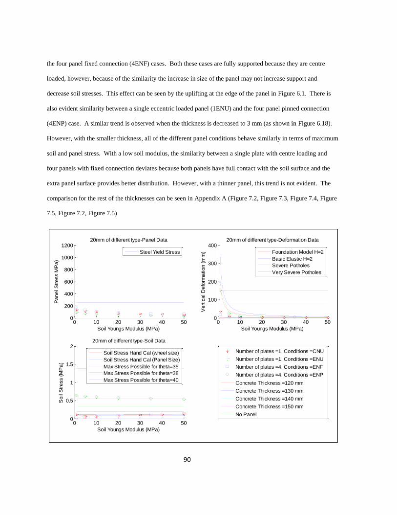
90
the four panel fixed connection (4ENF) cases. Both these cases are fully supported because they are centre
loaded, however, because of the similarity the increase in size of the panel may not increase support and
decrease soil stresses. This effect can be seen by the uplifting at the edge of the panel in Figure 6.1. There is
also evident similarity between a single eccentric loaded panel (1ENU) and the four panel pinned connection
(4ENP) case. A similar trend is observed when the thickness is decreased to 3 mm (as shown in Figure 6.18).
However, with the smaller thickness, all of the different panel conditions behave similarly in terms of maximum
soil and panel stress. With a low soil modulus, the similarity between a single plate with centre loading and
four panels with fixed connection deviates because both panels have full contact with the soil surface and the
extra panel surface provides better distribution. However, with a thinner panel, this trend is not evident. The
comparison for the rest of the thicknesses can be seen in Appendix A (Figure 7.2, Figure 7.3, Figure 7.4, Figure
7.5, Figure 7.2, Figure 7.5)
0 10 20 30 40 500
200
400
600
800
1000
120020mm of different type-Panel Data
Soil Youngs Modulus (MPa)
Pa
ne
l S
tre
ss M
Pa
)
Steel Yield Stress
0 10 20 30 40 500
100
200
300
40020mm of different type-Deformation Data
Soil Youngs Modulus (MPa)
Ve
rtic
al D
efo
rma
tio
n (
mm
)
Foundation Model H=2
Basic Elastic H=2
Severe Potholes
Very Severe Potholes
0 10 20 30 40 500
0.5
1
1.5
220mm of different type-Soil Data
Soil Youngs Modulus (MPa)
So
il S
tre
ss (
MP
a)
Soil Stress Hand Cal (wheel size)
Soil Stress Hand Cal (Panel Size)
Max Stress Possible for theta=35
Max Stress Possible for theta=38
Max Stress Possible for theta=40
Number of plates =1, Conditions =CNU
Number of plates =1, Conditions =ENU
Number of plates =4, Conditions =ENF
Number of plates =4, Conditions =ENP
Concrete Thickness =120 mm
Concrete Thickness =130 mm
Concrete Thickness =140 mm
Concrete Thickness =150 mm
No Panel
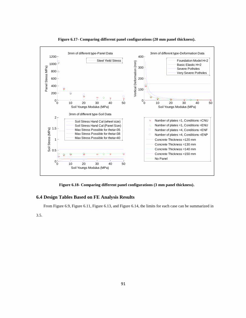
91
Figure 6.17- Comparing different panel configurations (20 mm panel thickness).
Figure 6.18- Comparing different panel configurations (3 mm panel thickness).
6.4 Design Tables Based on FE Analysis Results
From Figure 6.9, Figure 6.11, Figure 6.13, and Figure 6.14, the limits for each case can be summarized in
3.5.
0 10 20 30 40 500
200
400
600
800
1000
12003mm of different type-Panel Data
Soil Youngs Modulus (MPa)
Pa
ne
l S
tre
ss M
Pa
)
Steel Yield Stress
0 10 20 30 40 500
100
200
300
4003mm of different type-Deformation Data
Soil Youngs Modulus (MPa)
Ve
rtic
al D
efo
rma
tio
n (
mm
)
Foundation Model H=2
Basic Elastic H=2
Severe Potholes
Very Severe Potholes
0 10 20 30 40 500
0.5
1
1.5
23mm of different type-Soil Data
Soil Youngs Modulus (MPa)
So
il S
tre
ss (
MP
a)
Soil Stress Hand Cal (wheel size)
Soil Stress Hand Cal (Panel Size)
Max Stress Possible for theta=35
Max Stress Possible for theta=38
Max Stress Possible for theta=40
Number of plates =1, Conditions =CNU
Number of plates =1, Conditions =ENU
Number of plates =4, Conditions =ENF
Number of plates =4, Conditions =ENP
Concrete Thickness =120 mm
Concrete Thickness =130 mm
Concrete Thickness =140 mm
Concrete Thickness =150 mm
No Panel

92
Table 6.1- Summary Findings for all test cases.
1CNU 1ENU 4ENF 4ENF
Panel Stress
at 1 MPa - thickness >
=10 mm
at 5 MPa- Thickness >=
10mm
greater than 10 MPa –
thickness >= 1 mm
At 1 MPa- Thickness
>=10 mm
At 5 MPa- Thickness
>= 5 mm
At 10 MPa – thickness
>= 1 mm
At 1 MPa- thickness
>=15 mm
At 5 MPa- thickness
>= 10 mm
Greater than 10 MPa-
thickness >= 1 mm
At 1 MPa-
Thickness >=10
mm
At 5 MPa-
Thickness >= 5
mm
At 10 MPa –
thickness >= 1 mm
Deformation
At 1MPa – no trial
thickness
At 5 MPa – thickness
>=10 mm
greater than 10 MPa –
thickness >= 1 mm
At 10 MPa- thickness
>=1 mm
At 1 MPa- thickness
>=20 mm
At 5 MPa- 10 MPa
Greater than 10 MPa-
thickness >= 1 mm
At 10 MPa-
thickness >=1 mm
Soil Stress
At 1 MPa – Thickness
>= 10 mm
Greater than 5 MPa-
thickness >= 1 mm
Less than 5 MPa – no
Trial Thickness
At 5 MPa- thickness
<= 3mm
Greater than 10 MPa –
thickness >= 1mm
At 1 MPa- thickness
>= 10 mm
At 5 MPa- thickness
>= 1 mm
Less than 5 MPa –
no Trial Thickness
At 5 MPa-
thickness <= 3mm
Greater than 10
MPa – thickness
>= 1mm
To summarize the requirements of the two panels of different thicknesses, a 1 mm steel panel thickness will
hold all vertical truck loads without yielding the plate with 20 mm deformation, and there is no yielding in the
soil of a modulus 10 MPa and greater. A panel of 20 mm thickness is required for a soil modulus of 1 MPa
requiring the panel to be centre loaded and fixed without the soil yielding connection. This can be achieved by
creating a panel wider than the vehicle so that the load is to be closer to the center.
When the limits are simplified to the bearing capacity of the soil and the deformation allowable for
conventional pavement, the results can be presented in graphical form as shown in Figure 6.19. The results of
each test case are limited to the limited derived from section 3.5 and associated with the required thickness.
The graph in Figure 6.19 can be used as a design tool for selecting the steel panel thickness, given the soil
properties. The required soil properties are the elastic modulus and bearing capacity. To use Figure 6.19, the
soil at the location needs to be tested to determine these parameters. However, if testing cannot occur, Figure
6.19 gives approximate values for slip angles (which can be used to calculate bearing capacity) and soil moduli

93
corresponding to different soil types. Given the soil bearing capacity and soil elastic modulus, the
corresponding vertical and horizontal lines can be drawn. In the region in which the two corresponding lines
meet, the critical plate thickness is given. For example, a soil with a modulus of 20 MPa and a bearing capacity
of 0.25 MPa would require a steel panel thickness of 10 mm (as labeled as “#1” in Figure 6.19). When the
elastic modulus is 20 MPa and the bearing capacity is 0.05 MPa, the soil needs to be strengthened before a
panel can be applied. When the soil elastic modulus is 5 MPa and the soil bearing capacity is 0.25 MPa, a
stiffer soil is required. Soils can be strengthened and stiffened by introducing a subgrade material between the
panel and the native soil with the desired properties.
Figure 6.19- Panel design tool.
6.4.1 Load and Resistance Factors
In order to ensure that the panel design meets the safety requirements of the relevant codes, Figure 6.16 can
be modified to consider appropriate load and resistance factors. In the presented analysis, soil and panel failure
can be considered as ultimate limit states (ULS). Excess deformations can be considered as a serviceability
0 5 10 15 20 25 30 35 40 45 500
0.05
0.1
0.15
0.2
0.25
0.3
0.35
0.4
Soil Modulus (MPa)
So
il B
ea
rin
g C
ap
acity (
MP
a)
RequiresStiffening
of Soil
Requires Strenghtening andStiffening of Soil
Requires Strenghtening of Soil
Requires Panel Thickness 1 mm
Requires Panel Thickness 10 mm
Requires Panel Thickness 20 mm
30
32
34
36
Slip
An
gle
(d
eg
ree
)
Very Soft Soft Medium Stiff
Clay
Loose Dense
Sand
#1

94
limit state (SLS). Ultimate limit state defines the limits of the design based on material failure during peak
loads. Serviceability limit state defines the limits based on the functionality of the design during routine
loading. In the Canadian Bridge Code [Canadian Standards Association, 2006], a resistance factor of 0.5 is
suggested for soil failure. A resistance factor of 0.95 is suggested for steel.
Load factors provided in the Canadian Bridge Code. When only live loads are considered, a live load factor
of 1.7 is appropriate. In addition to this load factor, a dynamic load allowance (DLA) is applied to account for
the dynamic effects on the truck loading due to the fact that the truck is travelling at a considerable velocity.
With these load and resistance factors, we can update Figure 6.19. With the suggested factors of safety, a
modified panel guide is created (see Figure 6.20).
Table 6.2- Suggested factors of safety.
Variable Load and Resistance Factors Relevant Limit
State
Vehicle Loading 1.7 ULS
DLA 1.5 ULS/SLS
Soil Bearing
Capacity
0.5 ULS
Soil Elastic
Modulus
1.0 SLS
Steel Yield
Strength
0.95 ULS

95
Figure 6.20- Modified panel design tool.
6.4.2 Different Loading Conditions
Different loading conditions can also be explored, using a similar approach. The following are two
foreseeable truck loadings that can be tested: light and heavy vehicles. The first scenario shows the possibility
of decreasing the required panel thickness in order to make it more economical for private vehicle use. The
scenario with heavier vehicle loads shows the potential of the proposed system for the resource sector. Vehicles
in the resource sector are often heavier than normal trucks on conventional roadways. Fitch [Fitch, 1994]
described light trucks as having tire pressures of 40 psi (0.275 MPa). The United States Department of
Agriculture [Greenfield, 1993] defines the maximum tire pressure for logging vehicles as 100 psi (0.689 MPa).
With the two scenarios, we can modify the panel design tool for the different vehicle load applications.
Because of the elasticity of the metal, when the plates support a light truck load, the overall stresses and
deformation will be decreased by the ratio of the light truck load and normal truck load to 48%. Therefore, the
soil bearing capacity requirement will decrease by a factor of 48%, as seen in Figure 6.21, where the vertical
0 5 10 15 20 25 30 35 40 45 500
0.1
0.2
0.3
0.4
0.5
0.6
0.7
Soil Modulus (MPa)
So
il B
ea
rin
g C
ap
acity (
MP
a)
RequiresStiffening
of Soil
Requires Strenghtening andStiffening of Soil
Requires Strenghtening of Soil
Requires Panel Thickness 1 mm
Requires Panel Thickness 10 mm
Requires Panel Thickness 20 mm
3032
34
36
38
Slip
An
gle
(d
eg
ree
)
Very Soft Soft Medium Stiff
Clay
Loose Dense
Sand

96
positions of the curves are shifted with respect to those in Figure 6.19. When the load of a logging vehicle is
used, the requirement of the soil bearing capacity increases by 118%, as shown in Figure 6.22.
Figure 6.21- Modified Panel Design Guide for Light Trucks.
0 5 10 15 20 25 30 35 40 45 500
0.05
0.1
0.15
0.2
0.25
0.3
0.35
Soil Modulus (MPa)
So
il B
ea
rin
g C
ap
acity (
MP
a)
RequiresStiffening
of Soil
Requires Strenghtening andStiffening of Soil
Requires Strenghtening of Soil
Requires Panel Thickness 1 mm
Requires Panel Thickness 10 mm
Requires Panel Thickness 20 mm
30
32
34
36
Slip
An
gle
(d
eg
ree
)
Very Soft Soft Medium Stiff
Clay
Loose Dense
Sand
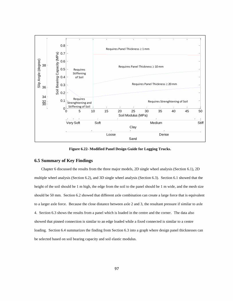
97
Figure 6.22- Modified Panel Design Guide for Logging Trucks.
6.5 Summary of Key Findings
Chapter 6 discussed the results from the three major models, 2D single wheel analysis (Section 6.1), 2D
multiple wheel analysis (Section 6.2), and 3D single wheel analysis (Section 6.3). Section 6.1 showed that the
height of the soil should be 1 m high, the edge from the soil to the panel should be 1 m wide, and the mesh size
should be 50 mm. Section 6.2 showed that different axle combination can create a large force that is equivalent
to a larger axle force. Because the close distance between axle 2 and 3, the resultant pressure if similar to axle
4. Section 6.3 shows the results from a panel which is loaded in the centre and the corner. The data also
showed that pinned connection is similar to an edge loaded while a fixed connected is similar to a centre
loading. Section 6.4 summarizes the finding from Section 6.3 into a graph where design panel thicknesses can
be selected based on soil bearing capacity and soil elastic modulus.
0 5 10 15 20 25 30 35 40 45 500
0.1
0.2
0.3
0.4
0.5
0.6
0.7
0.8
Soil Modulus (MPa)
So
il B
ea
rin
g C
ap
acity (
MP
a)
RequiresStiffening
of Soil
Requires Strenghtening andStiffening of Soil
Requires Strenghtening of Soil
Requires Panel Thickness 1 mm
Requires Panel Thickness 10 mm
Requires Panel Thickness 20 mm
3032
34
36
38
Slip
An
gle
(d
eg
ree
)
Very Soft Soft Medium Stiff
Clay
Loose Dense
Sand

98
Chapter 7
Conclusions and Recommendations
In the following sections, the main conclusions of the presented research are stated, and a number of areas
for future research on the subject of reusable, modular road plate systems are recommended.
7.1 Conclusions
The main conclusions of the research presented in the previous chapters are as follows:
Translating the empirical design rules for asphalt or concrete pavement to a modular road plate system is a
difficult task, as many of the empirical design criteria cannot be easily translated to a measurable structural
parameters such as a deflection or a stress. For this reason, mechanistic design methods are recommended for
the design of modular road plate systems.
The thickness of structural steel plate required to carry the vertical loads as Canadian highway traffic is
primarily a function of the soil properties, and to a lesser extent the loading and plate connection type (i.e.
boundary conditions). For various loading, soil, and boundary conditions, minimum plate thicknesses are
proposed, based on the FE analysis results.
Most of the observed failures for the investigated structural steel simple plate system were due to soil
strength limits being exceeded, rather than plate yielding or excessive deflection.
Hinged connections provide almost no benefit for resisting vertical, traffic-induced loads. Fixed connections
do result in a reduction in the predicted deflections and stresses.
An edge loaded plate, either alone or connected to adjacent plates with hinges, provides practically no benefit
in terms of reducing deflections or soil stresses under vertical, traffic-induced loads. In fact, the local soil
stresses at the plate edge can even be slightly higher in this case. For this reason, fixed connections should be
used or plate dimensions should be selected so that edge loading by a single wheel is not likely to occur. Plates
that are as wide as the roadway, and therefore likely to be loaded by two wheels simultaneously, are one
possibility.
99
The analysis of multi-plate systems can be simplified by modelling a single plate that is centre loaded (to
represent a multi-plate system with fixed plate connections) or a single plate that is edge loaded (to represent a
multi-plate system with hinged plate connections).
When the soil stiffness is high, failure is less dependent on the thickness of the panels and more dependent on
the shear angle of the soil (i.e. soil strength). When the soil stiffness is low, failure is more dependent on the
thickness of the panels, and failure by plate yielding dominates.
There should be three thicknesses for the manufactured panels (1 mm, 10 mm, and 20 mm) to accommodate
the wide range of soils in Canada. With the selective range, the product can be made cheaper for location with
firm soil properties. These panels should have fixed edge connections. The design chart for 87.5 kN truck from
Figure 6.20 shows which panel thickness is required for a given set of soil properties. Figure 6-21 and Figure
6.22 shows design guides for light trucks and logging truck, respectively.
7.2 Recommendations for Future Research
The following are recommendations for future research on reusable, modular road plate systems:
A detailed economic analysis for the proposed structural steel simple plate design is recommended. In this
analysis, the proposed system should be compared with current temporary road methods and current pavement
practices. A life-cycle cost analysis (LCCA) should be performed with a range of detour lengths and traffic
volumes.
A study on the effect of varying the plate dimensions in plan (i.e. width and length) is recommended. In
particular, non-square panel designs that span the entire road width should be investigated, as these might lead
to reduced edge load effects.
More sophisticated soil models should be introduced in future finite element (FE) analyses. These should
consider the possibility that local soil failure near the panel edge might not lead to failure of the plate system,
due to the short term nature of the loading and service life. Creep and cyclic loading effects could also be
considered with a more sophisticated soil model.
100
The FE analysis studies presented herein should be extended to other plate materials, including composite
plate systems (i.e. sandwich panels), and eventually to other modular road plate design concepts. This analysis
should be combined with an economic study to determine the optimal modular road plate system design for
different loading and soil conditions.
Structural analysis of the proposed system under horizontal, traffic induced loads (i.e. braking loads) is an
essential area for future research. These loads may have significant implications for the thinner plate designs,
the plate-to-plate connection design, and the design of the anchorage or gripping system, which may be required
to connect the plates to the soil.
Further evaluation is recommended of the proposed plate system with regards to other criteria defined in the
proposed methodology, such as skid resistance and durability.

101
Appendix A
Comparison of 3D FE Model Stresses
Figure 7.1- 20 mm Panel Thickness Comparison with Different Panel Configurations.
0 10 20 30 40 500
200
400
600
800
1000
120020mm of Different Type - Panel Data
Soil Elastic Modulus (MPa)
Pa
ne
l S
tre
ss M
Pa
)
0 10 20 30 40 500
50
100
150
20020mm of Different Type - Deformation Data
Soil Elastic Modulus (MPa)
Ve
rtic
al D
efo
rma
tio
n (
mm
)
0 10 20 30 40 500
0.2
0.4
0.6
0.820mm of Different Type - Soil Data
Soil Elastic Modulus (MPa)
So
il S
tre
ss (
MP
a)
Number of plates =1, Conditions =CNU
Number of plates =1, Conditions =ENU
Number of plates =4, Conditions =ENF
Number of plates =4, Conditions =ENP

102
Figure 7.2- 15 mm Panel Thickness Comparison with Different Panel Configurations.
Figure 7.3- 10 mm Panel Thickness Comparison with Different Panel Configurations.
0 10 20 30 40 500
200
400
600
800
1000
120015mm of Different Type - Panel Data
Soil Elastic Modulus (MPa)
Pa
ne
l S
tre
ss M
Pa
)
0 10 20 30 40 500
50
100
150
20015mm of Different Type - Deformation Data
Soil Elastic Modulus (MPa)
Ve
rtic
al D
efo
rma
tio
n (
mm
)
0 10 20 30 40 500
0.2
0.4
0.6
0.815mm of Different Type - Soil Data
Soil Elastic Modulus (MPa)
So
il S
tre
ss (
MP
a)
Number of plates =1, Conditions =CNU
Number of plates =1, Conditions =ENU
Number of plates =4, Conditions =ENF
Number of plates =4, Conditions =ENP
0 10 20 30 40 500
200
400
600
800
1000
120010mm of Different Type - Panel Data
Soil Elastic Modulus (MPa)
Pa
ne
l S
tre
ss M
Pa
)
0 10 20 30 40 500
50
100
150
20010mm of Different Type - Deformation Data
Soil Elastic Modulus (MPa)
Ve
rtic
al D
efo
rma
tio
n (
mm
)
0 10 20 30 40 500
0.2
0.4
0.6
0.810mm of Different Type - Soil Data
Soil Elastic Modulus (MPa)
So
il S
tre
ss (
MP
a)
Number of plates =1, Conditions =CNU
Number of plates =1, Conditions =ENU
Number of plates =4, Conditions =ENF
Number of plates =4, Conditions =ENP

103
Figure 7.4- 5 mm Panel Thickness Comparison with Different Panel Configurations.
Figure 7.5- 3 mm Panel Thickness Comparison with Different Panel Configurations.
0 10 20 30 40 500
200
400
600
800
1000
12005mm of Different Type - Panel Data
Soil Elastic Modulus (MPa)
Pa
ne
l S
tre
ss M
Pa
)
0 10 20 30 40 500
50
100
150
2005mm of Different Type - Deformation Data
Soil Elastic Modulus (MPa)
Ve
rtic
al D
efo
rma
tio
n (
mm
)0 10 20 30 40 50
0
0.2
0.4
0.6
0.85mm of Different Type - Soil Data
Soil Elastic Modulus (MPa)
So
il S
tre
ss (
MP
a)
Number of plates =1, Conditions =CNU
Number of plates =1, Conditions =ENU
Number of plates =4, Conditions =ENF
Number of plates =4, Conditions =ENP
0 10 20 30 40 500
200
400
600
800
1000
12003mm of Different Type - Panel Data
Soil Elastic Modulus (MPa)
Pa
ne
l S
tre
ss M
Pa
)
0 10 20 30 40 500
50
100
150
2003mm of Different Type - Deformation Data
Soil Elastic Modulus (MPa)
Ve
rtic
al D
efo
rma
tio
n (
mm
)
0 10 20 30 40 500
0.2
0.4
0.6
0.83mm of Different Type - Soil Data
Soil Elastic Modulus (MPa)
So
il S
tre
ss (
MP
a)
Number of plates =1, Conditions =CNU
Number of plates =1, Conditions =ENU
Number of plates =4, Conditions =ENF
Number of plates =4, Conditions =ENP

104
Bibliography
[All Terrain Road, 2005] All Terrain Road (2005). All Terrain Road Mats. Fluoro-Seal Interest, L.P.
[American Association of State Highway and Transportation Officials, 1993] American Association of State
Highway and Transportation Officials (1993). AASHTO Guide for Design of Pavement Structures. Number v. 2.
American Association of State Highway and Transportation Officials.
[American Association of State Highway and Transportation Officials, 2009] American Association of State
Highway and Transportation Officials (1993). AASTOWare- TaskForce Handbook. American Association of
State Highway and Transportation Officials.
[American Concrete Pavement Association, 2011] American Concrete Pavement Association (2011). StreetPave.
[American Society for Testing and Material, 2007] American Society for Testing and Material (2007). Standard
Specification for Manhole Cover Assembly, Bolted, Semi-Flush, Oiltight and Watertight, Hinged. American
Society for Testing and Materials, f1144 – 98 edition.
[Archondo-Callao and Faiz, 1994] Archondo-Callao, R. S. and Faiz, A. (1994). Estimating Vehicle Operating
Costs. World Bank Technical Paper Number 234.
[Ashby et al., 2007] Ashby, M., Shercliff, H., and Cebon, D. (2007). Materials: engineering, science, processing
and design. Butterworth-Heinemann.
[Balla, 1962] Balla, A. (1962). Balla, a. Balla, A, 88:13–34.
[Bekker, 1966] Bekker, M. (1966). Off-road locomotion on the moon and on earth. Journal of Terramechanics,
3(3):83–91. cited By (since 1996) 0.
[Bekker, 1972] Bekker, M. (1972). Closing remarks at a mobility symposium. Journal of Terramechanics, 8(4):69–
72. cited By (since 1996) 0.
[Bekker, 1974] Bekker, M. (1974). Accomplishments and future tasks in off-road transportation. Journal of
Terramechanics, 11(2):11–30. cited By (since 1996) 2.
[Beskou, 2011] Beskou, N.D., T.-D. (2011). Dynamic effects of moving loads on road pavements: A review. Soil
Dynamics and Earthquake Engineering, 31(4):547–567. cited By (since 1996) 0.
[Boussinesq, 1885] Boussinesq, J. (1885). Application des potentiels à l’étude de l’équilibre et du mouvement des
solides élastiques: principalement au calcul des deformations et des pressions que produisent, dans ces solides,
des efforts quelconques exercés sur une petite partie de leur surface ou de leur intérieur; mémoire suivi de
notes étendues sur divers points de physique mathématique et d’analyse. Gauthier-Villars.

105
[Burmister et al., 1943] Burmister, D. M., Palmer, L. A., and Barber, E. S. (1943). The theory of stress and
displacements in layered systems and applications to the design of airport runways. Highway Research Board
Proceedings, 23:126–148.
[Canadian Mat System Inc., 2011] Canadian Mat System Inc. (2011). FiberCon.
[Canadian Standards Association, 2006] Canadian Standards Association (2006). Canadian Highway Bridge
Design Code. National Standard of Canada Series. CSA International.
[Chong and Wrong, 1995] Chong, G. and Wrong, G. (1995). Manual for Condition Rating of Rigid Pavements:
Distress Manifestations. Ontario. Ministry of Transportation and Communications. Research and Development
Division.
[Chong et al., 1982] Chong, G., Wrong, G., of Transportation, O. M., Research, C., and Branch, D. (1982). Manual
for Condition Rating of Rigid Pavements: Concrete Surface and Composite Distress Manifestations. The
Research and Development Branch Ministry of Transportation, Ontario.
[Danielson et al., 1996] Danielson, K. T., Noor, A. K., and Green, J. S. (1996). Computational strategies for tire
modeling and analysis. Computers & Structures, 61(4):673 – 693.
[Das, 2009] Das, B. (2009). Principles of Geotechnical Engineering: SI Version. Cengage Learning.
[Environment Canada, 2008] Environment Canada (2008). Adapting to climate change. EnviroZine, 87.
[Environment Canada, 2010] Environment Canada (2010). Weather - Environment Canada. Website.
[Eventsystems, 2011] Eventsystems (2011). ROLLAROAD.
[Fan et al., 2011] Fan, H. b., Liu, F., and Long, H. (2011). Locomotion of vehicles on hinged road mats. Journal of
Terramechanics, 48(1):47–55..
[Fitch, 1994] Fitch, J. (1994). Motor truck engineering handbook. Society of Automotive Engineers.
[Flowers et al., 2010] Flowers, J. N., Zech, W. C., and Abbas, H. H. (2010). Rapid bridge deck replacement
construction techniques: State of the practice. Number 2152 in Transportation Research Record. Transportation
Research Record.
[Frisch and Christophersen, 1964] Frisch, R. and Christophersen, R. (1964). Theory of Production. Springer.
[Gartrell, 2009] Gartrell, C.A., Newman, J.K., Anderton, G.L (2009). Performance measurements of pavement
matting systems by full-scale testing over differing soil strengths. Journal of Materials in Civil Engineering,
21(10):561–568.
[Gerrard, 2000] Gerrard, J. (2000). Fundamentals of Soils. Routledge fundamentals of physical geography series.
Routledge.

106
[Greene et al., 2010] Greene, J., Toros, U., and Choubane, B. (2010). Impact of wide-base single tires on pavement
damage. Transportation Research Record, (2155):82–90. cited By (since 1996) 1.
[Greenfield, 1993] Greenfield, P. H. (1993). Central tire inflation: USDA forest service program. In Engineering
Field Notes, volume 24, page 3. United States Department of Agriculture: Forest Service.
[Gunaratne, 2006] Gunaratne, M. (2006). The foundation engineering handbook. CRC/Taylor & Francis.
[Hansen, 1970] Hansen, J. B. (1970). A revised and extended formula for bearing capacity. Danish Geotechnical
Institute, 28.
[Helwany, 2007] Helwany, S. (2007). Applied soil mechanics: with ABAQUS applications. John Wiley & Sons.
[Hodgson, 1999] Hodgson, A. (1999). Self-aligning hinge.
[Huang, 1993] Huang, Y. (1993). Pavement analysis and design. Prentice Hall.
[Ioannides, 1992] Ioannides, A M., Salsilli, R A., Vinding, I., Packard, R G. (1992). Super-singles: Implications for
design. Heavy Vehicles and Roads: Technology, Safety and Policy. Proceedings of the Third International
Symposium on Heavy Vehicle Weights and Dimensions, 28 June - 2 July 1992, Queen’s College Cambridge,
UK, 28:225–32.
[Keeling, 1947] Keeling, R. C. (1947). Design of flexible pavement using the triaxial compression test. Highway
Research Board Bulletin, 8:33.
[Kim and Tutumluer, 2008] Kim, M. and Tutumluer, E. (2008). Multiple wheel-load interaction in flexible
pavements. Transportation Research Record, (2068):49–60.
[Kurtay and Reece, 1970] Kurtay, T. and Reece, A. (1970). Plasticity theory and critical state soil mechanics.
Journal of Terramechanics, 7(3-4):23–56.
[Lundgren and Mortensen, 1953] Lundgren, H. and Mortensen, K. (1953). Determination by the theory of plasticity
of the bearing capacity of continuous footings on sand. Proceedings of the 3rd International Conference on Soil
Mechanics and Foundation Engineering, 1:409–412.
[Lynch et al., 1999] Lynch, L., Jano, V., and Horne, D. (1999). U.S. Army corps of engineers experience with
accelerated and full-scale pavement investigations. Technical memorandum no. 3-37, USAE Waterways
Experiment Station, Vicksburg, MS. Technical Memorandum No. 3-37.
[Mallick and El-Korchi, 2009] Mallick, R. and El-Korchi, T. (2009). Pavement engineering: principles and
practice. CRC Press.
[Manitoba Conservation and Water Stewardship, 2012] Manitoba Conservation and Water Stewardship (2012).
FORESTRY ROAD MANAGEMENT. Manitoba Conservation and Water Stewardship.

107
[Melnick and Melnick, 1994] Melnick, M. and Melnick, R. (1994). Manhole Covers. MIT Press.
[Meyerhof, 1953] Meyerhof, G. G. (1953). The bearing capacity of foundations under eccentric and inclined loads.
Third International Conference on Soil Mechanics and Foundation Engineering, 1:440 – 445.
[Murphy, 2009] Murphy, C. (2009). ISO, the International Organization for Standardization: Global Governance
through Voluntary Consensus. Global Institutions Series. Taylor & Francis.
[Najafi and Gokhale, 2005] Najafi, M. and Gokhale, S. (2005). Trenchless technology: pipeline and utility design,
construction, and renewal. McGraw-Hill.
[Nasvik, 2005] Nasvik, J. (2005). Working with gang forms. Concrete Construction - World of Concrete, 50(8):30–
34.
[Poli, 2001] Poli, C. (2001). Design for Manufacturing: A Structured Approach. Elsevier Science.
[Popov, 1991] Popov, E. P. (1991). Engineering Mechanics of Solids. Prentice-Hall.
[Prabhu et al., 2009] Prabhu, M., Varma, A., and Buch, N. (2009). Analytical investigation of the effects of dowel
misalignment on concrete pavement joint opening behaviour. International Journal of Pavement Engineering,
10(1):49–62.
[Robinson et al., 2011] Robinson, T., Armstrong, C., and Fairey, R. (2011). Automated mixed dimensional
modelling from 2d and 3d cad models. Finite Elements in Analysis and Design, 47(2):151 – 165.
[Simulia, 2007] Simulia (2007). Abaqus: Version 6.7. Simulia.
[Society of Petroleum Engineers (U.S.), 1991] Society of Petroleum Engineers (U.S.) (1991). Horizontal Drilling.
S P E REPRINT SERIES BOOKLETS. Society of Petroleum Engineers.
[Sun and Sacks, 2005] Sun, W. and Sacks, M. (2005). Finite element implementation of a generalized fung-elastic
constitutive model for planar soft tissues. Biomechanics and Modeling in Mechanobiology, 4:190–199.
10.1007/s10237-005-0075-x.
[Takata and Umeda, 2007] Takata, S. and Umeda, Y. (2007). Advances in life cycle engineering for sustainable
manufacturing businesses: proceedings of the 14th CIRP Conference on Life Cycle Engineering, Waseda
University, Tokyo, Japan, June 11th-13th, 2007. Springer.
[Texas Department of Transportation, 2011] Texas Department of Transportation (2011). Pavement Design Guide.
Texas Department of Transportation.
[Transportation Association of Canada, 2012] Transportation Association of Canada (2012). Pavement Asset
Design and Management Guide. Transportation Association of Canada.
108
[Uzarowski, 2006] Uzarowski, L. (2006). The Development of Asphalt Mix Creep Parameters and Finite Element
Modeling of Asphalt Rutting. PhD thesis, University of Waterloo.
[Vesic, 1973] Vesic, A. S. (1973). Analysis of ultimate loads of shallow foundations. Journal of the Soil Mechanics
and Foundations Division, 99:45–73.
[Wang, 2010] Wang, F.and Liu, K. W. X.-C. (2010). Impact analysis for computer simulating multi-factor on
cement slab deflection. In Impact analysis for computer simulating multi-factor on cement slab deflection,
volume 3, pages 528–532, Sanya.; Conference of 2010 International Conference on Computer Modeling and
Simulation, ICCMS 2010; Conference Date: 22 January 2010 through 24 January 2010; Conference Code:
79952.
[Webster and Tingle, 1998] Webster and Tingle (1998). Expedient road construction over sands using lightweight
mats. Report, U.S. Army Corps of Engineers, Waterways Experiment Station.
[Wong, 2009] Wong, J. (2009). Terramechanics and off-road vehicle engineering: terrain behaviour, off-road
vehicle performance and design. Elsevier Science & Technology.
[Young et al., 2004] Young, H., Freedman, R., Ford, A., and Sears, F. (2004). Sears and Zemansky’s university
physics: with modern physics. Pearson Addison Wesley.
[Zienkiewicz et al., 2005] Zienkiewicz, O., Taylor, R., and Nithiarasu, P. (2005). The Finite Element Method.
Butterworth-Heinemann.