monday, session md-1, siirola

Sandia National Laboratories is a multi-program laboratory managed and operated by Sandia Corporation, a wholly owned subsidiary of Lockheed Martin Corporation, for the U.S. Department of Energy's

National Nuclear Security Administration under contract DE-AC04-94AL85000.

Leveraging Block-Composable Optimization Modeling Environments for Transmission

Switching and Unit Commitment

John D. Siirola,1 Jean-Paul Watson,1 and David L. Woodruff 2

1 Discrete Math & Complex Systems Department Sandia National Laboratories

Albuquerque, NM USA

2 Graduate School of Management University of California, Davis

Davis, CA USA

Increasing Real-Time and Day-Ahead Market Efficiency through Improved Software 25 June 2012

Siirola, Watson, Woodruff, p. 2

This is a talk on modeling environments• Our premise:

– Optimization (math programming; MP) is critical for grid planning and operations

– Typical models are tough to create and tougher to understand– We increasingly leverage problem-specific structure to solve

harder (bigger, more complex) problems effectively

• Our approach:– New MP modeling environment (Pyomo)

• Extensible: new modeling constructs• Powerful: develop new native solvers, heuristic methods• Open: (1) transparent;

solvers, heuristics, etc. can interrogate and manipulate model• Open: (2) freely distributable;

researchers, vendors, operators can share models


The Challenge: MP is dense and subtle

Hedman, et al., "Co-Optimization of Generation Unit Commitment and Transmission Switching With N-1 Reliability," IEEE Trans Power Systems, 25(2), pp.1052-1063, 2010


The Challenge: MP is dense and subtle

Hedman, et al., "Co-Optimization of Generation Unit Commitment and Transmission Switching With N-1 Reliability," IEEE Trans Power Systems, 25(2), pp.1052-1063, 2010

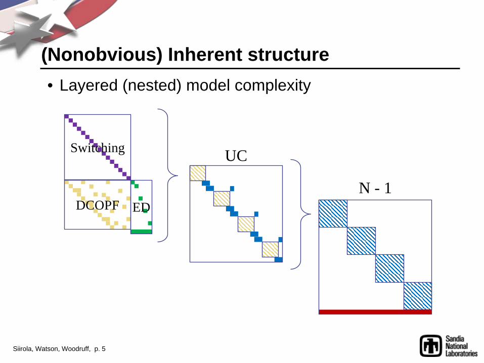
To a first approximation:- DCOPF- Economic dispatch- Unit commitment- Transmission switching- N-1 contingency


(Nonobvious) Inherent structure• Layered (nested) model complexity

DCOPF ED

Switching UC

N - 1


Block-oriented modeling• “Blocks”

– Collections of model components• Var, Param, Set, Constraint, etc.

– Blocks may be arbitrarily nested

• Why blocks?– Support reusable modeling components– Express distinctly modeled concepts as distinct objects– Manipulate modeled components as distinct entities– Explicitly expose model structure (e.g., for decomposition)

• Prior art– Ubiquitous in the simulation community– Rare in Math Programming environments

• Notable exceptions: ASCEND, JModelica.org


GLPK

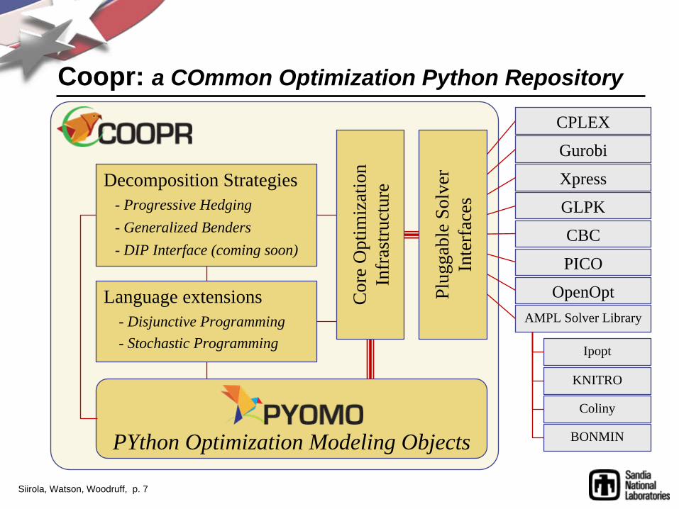
PYthon Optimization Modeling Objects

Coopr: a COmmon Optimization Python Repository

Language extensions- Disjunctive Programming- Stochastic Programming

Decomposition Strategies- Progressive Hedging- Generalized Benders- DIP Interface (coming soon)

CPLEX

Gurobi

Xpress

AMPL Solver Library

CBC

PICO

OpenOptPlug

gabl

e So

lver

In

terf

aces

Cor

e O

ptim

izat

ion

Infr

astru

ctur

e

Ipopt

KNITRO

Coliny

BONMIN


from coopr.pyomo import *

m = ConcreteModel()

m.x1 = Var()m.x2 = Var(bounds=(-1,1))m.x3 = Var(bounds=(1,2))

m.obj = Objective( sense = minimize,expr = m.x1**2 + (m.x2*m.x3)**4 +

m.x1*m.x3 + m.x2 +m.x2*sin(m.x1+m.x3) )

model = m

Pyomo overview• Formulating optimization models natively within Python

– Provides a natural syntax to describe mathematical models– Can formulate large models with a concise syntax– Separates modeling and data declarations– Enables data import and export in commonly used formats

• Highlights:– Clean syntax– Python scripts provide

a flexible context for exploring the structure of Pyomo models

– Leverage high-quality third- party Python libraries, e.g., SciPy, NumPy, MatPlotLib


• Capture connected block structure, e.g., network flow

• Block interface through connectors (group of variables)• Block implementation independent of network definition

Domain Node Arc Connector Vars

Fluid flow Mass balance Pressure Drop Pressure; Volumetric flow

AC Power flow KCL Active power transfer;Reactive power transfer

Phase angle;Active power flow;Reactive power flow

Structured modeling with blocks

Node

ArcArc

Arc Arc

Arc

Node

Node Node

Node

Node


DC OPF: transmission (line) modeldef dc_line_rule(line, id):

line.B = Param()

line.Limit = Param()

line.V_angle_in = Var()

line.V_angle_out = Var()

line.Power = Var( bounds= ( -line.Limit, line.Limit ) )

line.power_flow = Constraint( expr= \

line.Power == line.B*(line.V_angle_in - line.V_angle_out) )

line.IN = Connector( initialize= \

{ “Power”: -line.Power, “V_angle”: line.V_angle_in } )

line.OUT = Connector( initialize= \

{ “Power”: line.Power, “V_angle”: line.V_angle_out } )


General power flow model (1 / 2)from coopr.pyomo import *

model = AbstractModel()

model.BUSES = Set()

model.LINES = Set()

model.GENERATORS = Set()

model.ENDPOINTS = Set(initialize=[“IN”, “OUT”])

model.links = Param( model.LINES, model.ENDPOINTS )


General power flow model (2 / 2)

from power_flow import \

dc_line_rule as line_rule, \

dc_bus_rule as bus_rule, \

dc_generator_rule as generator_rule

model.bus = Block( model.BUSES, rule=bus_rule )

model.line = Block( model.LINES, rule=line_rule )

model.generator = Block( model.GENERATORS, rule=generator_rule )

def _network(model, l, end):

if endpoint == ‘IN’:

return model.line[l].IN == model.bus[ value(model.links[l, end]) ].PORT

else:

return model.line[l].OUT == model.bus[ value(model.links[l, end]) ].PORT

model.network = Constraint(model.LINES, model.ENDPOINTS, rule=_network)

def _generator_placement(model, g):

return model.generator[g].OUT == model.bus[ value(model.generator[g].bus) ].PORT

model.generator_placement = Constraint(model.GENERATORS, rule=_generator_placement)

Only domain-specific component( Note: we have only shown the line rule and not the bus or generator rules )


Solving block models1) Construct hierarchical model

– Generate blocks (Variables + Internal constraints)– “Connect” blocks by forming constraints over block connectors

2) Use a model transformation to “flatten” the model– Replicates connector constraints for each variable in connector– Generates aggregating constraints– (Eliminates redundant variables)


from power_flow import ac_line_rule as line_rule, \

ac_bus_rule as bus_rule, \

ac_generator_rule as generator_rule







else:






Model libraries: switching to ACOPF is trivial


Manipulating model blocks• Generalized Disjunctive Programming (GDP)

– Switching entire blocks on/off through binary variables

• Introduce new modeling components:– “Disjunct”

• a new form of model block– “Disjunction”

• a new constraint for enforcing logical XOR over disjunctive sets

min ck f x k

s.t. g x 0

iDk

VYik

hik x o

ck ik

Y trueYik {true, false}


Creating an “open line” modeldef open_dc_line_rule(line):



line.Power = Var()

line.power_flow = Constraint( expr= line.Power == 0 )


{ “Power”: -line.Power, “V_angle”: line.V_angle_in } )


{ “Power”: line.Power, “V_angle”: line.V_angle_out } )


Creating a “switchable line”def switchable_dc_line_rule(line, id):



line.Power_in = Var()

line.Power_out = Var()


{ “Power”: line.Power_in, “V_angle”: line.V_angle_in } )


{ “Power”: line.Power_out, “V_angle”: line.V_angle_out } )

line.Closed = Disjunct( rule=dc_line_rule )

line.Open = Disjunct ( rule=open_dc_line_rule )

line.Switch = Disjunction( initialize=[line.Closed, line.Open] )

line.connections = ConstraintList()

for block in ( line.Open, line.Closed ):

line.connections.add( line.IN = block.IN )

line.connections.add( line.OUT = block.OUT )


from power_flow import switchable_dc_line_rule as line_rule, \

dc_bus_rule as bus_rule, \

dc_generator_rule as generator_rule







else:






Creating a transmission switching model


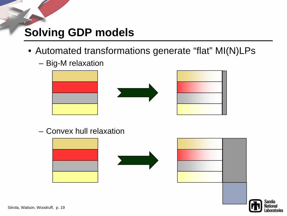
Solving GDP models• Automated transformations generate “flat” MI(N)LPs

– Big-M relaxation

– Convex hull relaxation


def dc_economic_dispatch_rule(b, *args):

b.bus = Block( b.model().BUSES, rule=bus_rule )

b.line = Block( b.model().LINES, rule=line_rule )

b.generator = Block( b.model().GENERATORS, rule=generator_rule )

def _network(b, l, end):


return b.line[l].IN == b.bus[ value(b.model().links[l, end]) ].PORT

else:

return b.line[l].OUT == b.bus[ value(b.model().links[l, end]) ].PORT

ed.network = Constraint(b.model().LINES, b.model().ENDPOINTS, rule=_network)

def _gen_placement(b, g):

return b.generator[g].OUT == b.bus[ value(b.generator[g].bus) ].PORT

b.generator_placement = Constraint(b.model().GENERATORS, rule=_gen_placement)

Convert transmission model block rule


from power_flow import dc_economic_dispatch_rule

model.TIMES = SET()

model.period = Block( model.TIMES, rule=dc_economic_dispatch_rule )

def _gen_limit(model, t, g):

if t == 1:

return Constraint.Skip

else:

return model.period[t-1].generator[g].STATE == \

model.period[t].generator[g].PREV_STATE

model.generation_limit = Constraint(model.TIMES, model.GENERATORS, rule=_gen_limit)

Generate the UC model

Note: the generator ramp limits and startup / shutdown constraints are part of a “switchable generator” block similar to the “switchable line” block. This is a complex block (13+ parameters, 8+ variables, 7+ constraints), and is completely abstracted away by the block modeling approach.


Exploiting block structure: decomposition• “Block diagonal” models very common in optimization

– Stochastic programming– Parameter estimation– Design enumeration (e.g., N-1)

M(x1 ,y1 )

…

N(y)

M

M,N

M(x1 ,y1 )

…

+ magic to converge

N(y)

M(x2 ,y2 )

M(xn ,yn )

M(x2 ,y2 )

M(xn ,yn )


Putting it together: UC + switching + N-1

~~

~

~

N-1 Contingencies

Unit Commitment

DecisionsSwitchable Transmission Line

Network Model

Bus model

Generator Model

Current Balance (KCL)

Transmission Line Power Flow Model

V

Generation Model

Ramp Limits (

V

Presenter

Presentation Notes

def switchable_line(model, line): line.pf_model = Block(rule=DC_line_model) line.IN = Connector(dup=line.pf_model.IN) line.OUT = Connector(dup=line.pf_model.OUT) def active_rule(model, disjunct): disjunct.line_in = Constraint( expr=line.IN == line.pf_model.IN ) disjunct.line_in = Constraint( expr=line.OUT == line.pf_model.OUT ) line.active = Disjunct(rule=active_rule) def inactive_rule(model, disjunct): disjunct.line_in = Constraint( expr=line.IN == model.NO_FLOW ) disjunct.line_in = Constraint( expr=line.OUT == model.NO_FLOW ) line.inactive = Disjunct(rule=inactive_rule) line.switch = Disjunction( expr=[line.active, line.inactive] )


“Blocks” fundamentally change modeling• Explicit model blocks

– Component reuse– Implicit transformations when generating model instances

• Generalized Disjunctive Programs– Explicit transformations to create standard forms– (Solver-specific decomposition)

• Block diagonal models– Implicit transformation to create standard forms– Solver-specific decomposition


Acknowledgements• Sandia National Laboratories

– Bill Hart– Jean-Paul Watson– John Siirola– David Hart– Tom Brounstein

• University of California, Davis– Prof. David L. Woodruff– Prof. Roger Wets

• Texas A&M University– Prof. Carl D. Laird– Daniel Word– James Young– Gabe Hackebeil

• Texas Tech University– Zev Friedman

• Rose Hulman Institute – Tim Ekl

• William & Mary– Patrick Steele

• North Carolina State– Kevin Hunter

Plus our many users, including:- University of California, Davis- Texas A&M University- University of Texas- Rose-Hulman Institute of Technology- University of Southern California- George Mason University- Iowa State University- N.C. State University- University of Washington- Naval Postgraduate School- Universidad de Santiago de Chile - University of Pisa - Lawrence Livermore National Lab- Los Alamos National Lab


For more information…

• Project homepage– http://software.sandia.gov/coopr

• “The Book”

• Mathematical Programming Computation papers– Pyomo: Modeling and Solving Mathematical Programs in Python (Vol. 3, No. 3, 2011)– PySP: Modeling and Solving Stochastic Programs in Python (Vol. 4, No. 2, 2012)

monday, session md-1, siirola

Documents