monetary policy across space and time -...
TRANSCRIPT
Monetary Policy across Space and Time∗
Laura Liu† Christian Matthes‡ Katerina Petrova§
October 10, 2018
Abstract
In this paper we ask two questions: (i) is the conduct of monetary policy stable across time
and similar across major economies, and (ii) do policy decisions of major central banks have
international spillover effects. To address these questions, we build on recent semi-parametric
advances in time-varying parameter models that allow us to increase the VAR dimension and to
jointly model three advanced economies (US, UK, and the Euro Area). Our main reduced-form
finding is an increased connectedness between and within countries during the recent financial
crisis. In order to study policy spillovers, we jointly identify three economy-specific monetary
policy shocks using a combination of sign and magnitude restrictions. We find that monetary
policy shocks were larger in magnitude and more persistent in the early 1980s than in subsequent
periods. We also uncover positive spillover effects of policy between countries in the 1980s and
diminished, and sometimes negative ‘beggar-thy-neighbour’ effects in the second half of the
sample. Moreover, during the 1980s, we find evidence for policy coordination between central
banks.
JEL codes: C54, E30, E58
Keywords: Monetary policy spillovers, time-varying parameters, changing volatility
∗We would like to thank Thomas Lubik as well as workshop participants at the EUI workshop on time-varying
parameter models and the St. Andrews Workshop on time-varying uncertainty in macro. The views expressed in
this paper are those of the authors and do not necessarily reflect those of the Federal Reserve Board of Governors,
the Federal Reserve Bank of Richmond, or the Federal Reserve System.†Federal Reserve Board of Governors, Email: [email protected]‡Federal Reserve Bank of Richmond, Email: [email protected]§University of St. Andrews, Email: [email protected]
1
1 Introduction
The past 50 years have seen three major economic events that have been shared across many indus-
trialized economies: the Great In�ation of the late 1970s and early 1980s, the Great Moderation
starting in the mid-1980s, and the 2008 �nancial crisis and the subsequent recession. In this pa-
per we use macroeconomic time series for three major world economies (the Euro Area, the US,
and the UK) that feature these key events as a backdrop to ask what the conduct and e¤ects of
monetary policy have been, how they have changed over time, and whether they have been similar
across these economies. A question of particular importance for monetary policy concerns policy
spillovers: do macroeconomic variables in major economies react to decisions of central banks in
other major economies? Our choice of countries is motivated by the fact that the selected economies
account for more than a third of total world GDP. Even though they all share the historic episodes
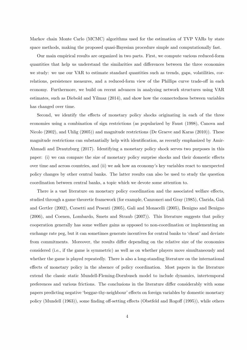
mentioned before, the magnitude of these events has been dramatically di¤erent, as illustrated in
Figure 1: the Great In�ation was most severe in the UK, while the Bundesbank, which later joined
the European Central Bank (ECB), is often credited with avoiding the large spikes in in�ation
we have seen in the other two countries. The Great Moderation period, characterized by low and
stable in�ation and unemployment, arrived later in the UK than in the US. Finally, the recession
after the recent �nancial crisis and the associated recovery followed a very di¤erent path in the
Euro Area (EA).
In this paper, we estimate a time-varying parameter model with drifting volatility using a semi-
parametric approach to investigate monetary policy experiences across countries and during the
three major events described above. We jointly identify three economy-speci�c monetary policy
shocks and investigate the spillover e¤ects of policy across countries and time. To this end, we
employ a combination of sign and magnitude restrictions, leaving most variables�responses unre-
stricted, and letting the data speak on their direction and size.
The motivation behind our modeling choice is that vector autoregressive (VAR) models are
well-suited for answering our research questions, as they allow for modeling interconnectedness and
joint dynamics of macroeconomic time series. However, ignoring the structural changes and breaks
in the past few decades that are both evident in the data and documented in the literature, can
result in invalid inference; hence, allowing for time-variation in the parameters and volatility of
the VAR model is essential. Because of the multi-country connections we want to explore, we also
require a relatively large number of observables in the VAR model alongside parameter drift.
2
Figure 1: Unemployment, In�ation and Interest Rates across countries
Time-varying parameter (TVP) VAR models have been made popular by Cogley and Sargent
(2005) and Primiceri (2005). One concern of the model speci�cation popularized in these papers is
that it is generally not amenable to having more than a few variables in the VAR (the upper bound
in the literature seems to be around �ve, as used, for example, in Amir-Ahmadi, Matthes and Wang
(2016)) and few lags (the standard choice seems to be two lags for quarterly data, as in Cogley and
Sargent (2005) and Primiceri (2005)). The reason for this concern is that state space methods used
to �lter the drifts in the parameters are subject to the �curse of dimensionality�which is particularly
severe when considering richly parameterized VAR models. This prevents researchers from using
larger datasets that have been employed and found important in �xed-coe¢ cient VARs (see, for
example, Christiano, Eichenbaum and Evans (1999)).
To handle a larger number of drifting parameters, we use the quasi-Bayesian local likelihood
approach to estimate time-varying parameter VARs introduced in Petrova (2018). The combination
of the closed-form quasi-posterior expressions derived in Petrova (2018) with standard Minnesota-
type priors used in the literature on �xed-coe¢ cient VARs speci�ed directly on the drifting para-
meters, allows the number of variables in the VAR to be large while also facilitating the parameter
drift. Moreover, the quasi-Bayesian local likelihood approach of Petrova (2018) models the parame-
ter time-variation nonparametrically, ensuring consistent estimation in a wide class of parameter
processes and alleviating the risk of invalid inference due to misspecifying the state equations for
the latent parameters in random coe¢ cient models. Finally, the availability of analytic expressions
for the quasi-posterior density in the Gaussian VAR case eliminates the computational burden of
3
Markov chain Monte Carlo (MCMC) algorithms used for the estimation of TVP VARs by state
space methods, making the proposed quasi-Bayesian procedure simple and computationally fast.
Our main empirical results are organized in two parts. First, we compute various reduced-form
quantities that help us understand the similarities and di¤erences between the three economies
we study: we use our VAR to estimate standard quantities such as trends, gaps, volatilities, cor-
relations, persistence measures, and a reduced-form view of the Phillips curve trade-o¤ in each
economy. Furthermore, we build on recent advances in analyzing network structures using VAR
estimates, such as Diebold and Yilmaz (2014), and show how the connectedness between variables
has changed over time.
Second, we identify the e¤ects of monetary policy shocks originating in each of the three
economies using a combination of sign restrictions (as popularized by Faust (1998), Canova and
Nicolo (2002), and Uhlig (2005)) and magnitude restrictions (De Graeve and Karas (2010)). These
magnitude restrictions can substantially help with identi�cation, as recently emphasized by Amir-
Ahmadi and Drautzburg (2017). Identifying a monetary policy shock serves two purposes in this
paper: (i) we can compare the size of monetary policy surprise shocks and their domestic e¤ects
over time and across countries, and (ii) we ask how an economy�s key variables react to unexpected
policy changes by other central banks. The latter results can also be used to study the question
coordination between central banks, a topic which we devote some attention to.
There is a vast literature on monetary policy coordination and the associated welfare e¤ects,
studied through a game theoretic framework (for example, Canzoneri and Gray (1985), Clarida, Gali
and Gertler (2002), Corsetti and Pesenti (2005), Gali and Monacelli (2005), Benigno and Benigno
(2006), and Coenen, Lombardo, Smets and Straub (2007)). This literature suggests that policy
cooperation generally has some welfare gains as opposed to non-coordination or implementing an
exchange rate peg, but it can sometimes generate incentives for central banks to �cheat�and deviate
from commitments. Moreover, the results di¤er depending on the relative size of the economies
considered (i.e., if the game is symmetric) as well as on whether players move simultaneously and
whether the game is played repeatedly. There is also a long-standing literature on the international
e¤ects of monetary policy in the absence of policy coordination. Most papers in the literature
extend the classic static Mundell-Fleming-Dornbusch model to include dynamics, intertemporal
preferences and various frictions. The conclusions in the literature di¤er considerably with some
papers predicting negative �beggar-thy-neighbour�e¤ects on foreign variables by domestic monetary
policy (Mundell (1963)), some �nding o¤-setting e¤ects (Obstfeld and Rogo¤ (1995)), while others
4
predicting positive �complementary�spillover e¤ects (Corsetti and Pesenti (2001)). The results in
the literature are largely determined by the relative strength of the di¤erent transmission channels
of monetary policy (exchange rate, terms of trade, or current account channels) imposed through
the theoretical assumptions as well as the parameter calibrations of the models in these papers.
Because there is a lack of clear consensus in the literature on the direction of policy spillover
e¤ects and coordination of monetary policy, our approach is useful as it imposes fewer theoretical
restrictions and lets the data speak, while also allowing for the possibility that these e¤ects might
be changing over time.
The empirical macroeconomic literature that has touched upon some of our research questions
includes Lubik and Schorfheide (2006), Gerko and Rey (2017), Stephane, Pesaran, Smith and Smith
(2013), to name a few. For example, Gerko and Rey (2017) compare the e¤ects of monetary policy
shocks across the UK and US and �nd that the spillover e¤ects are stronger from the US to the
UK than vice versa. Gerko and Rey (2017) are silent on how these e¤ects have varied over time,
a focus of our paper. Papers that study how much co-movement there is across major economies
include Canova, Ciccarelli and Ortega (2007) and Billio, Casarin, Ravazzolo and Van Dijk (2016).
The latter studies a sample that includes the �nancial crisis and �nds, similar to our results,
stronger co-movement in that period compared to earlier periods (focusing on the US and the EA
only). Concerning monetary policy, some papers have analyzed di¤erences in the 1970s: DiCecio
and Nelson (2009) emphasize similarities between the conduct of US and UK monetary policy
in the 1970s, whereas Beyer, Gaspar, Gerberding and Issing (2008) emphasize large di¤erences
in estimated policy rules between the US, UK, and Germany during that period. Most of the
empirical literature either estimates a �xed-parameter VAR or DSGE model, typically considering
a smaller subset of the sample to avoid estimation bias stemming from the structural change in the
series, or estimates a time-varying model either through considering a small number of variables,
possibly at the cost of omitted variable bias, or by imposing some additional (factor/ Markov-
switching) structure on the parameter time-variation. The advantage of our approach is that we
model jointly the three economies using a larger variable set and longer sample, while also allowing
for time-variation in the dynamics of all variables.
Our main reduced-form result is that once we allow for drifts in the model�s parameters, we
�nd signi�cant time-variation in the cross-country interconnectedness, based on weighted directed
networks constructed as in Diebold and Yilmaz (2014). Particularly, connectedness of economic
and �nancial variables within and between countries is smaller during the Great Moderation and
5
increases considerably during the recent �nancial crisis, making spillover from �nancial to real
variables as well as cross-country contagion much more severe. Our monetary policy shock analysis
suggests several conclusions. First, monetary policy shocks are larger in magnitude and more
persistent in the Great Moderation than in any subsequent periods in all economies. Second, we
�nd positive spillover e¤ects of policy across countries in the 1980s (particularly from the EA to US
and UK, as well as from US to UK and from UK to US) as well as evidence for policy coordination
during that period, and smaller and sometimes negative �beggar-thy-neighbour� spillover e¤ects
and no coordination in the subsequent periods. Third, while we impose that the e¤ects of foreign
monetary policy shocks are smaller on impact than domestic policy shocks, foreign spillovers can
occasionally have more persistent e¤ects.
The remainder of the paper is organized as follows. Section 2 outlines the Bayesian semi-
parametric methodology utilized in the paper and provides a brief comparison with alternative
methods. Section 3.1 contains a detailed description of the model speci�cation, data, and priors.
Sections 3.2 and 3.3 present the reduced-form empirical results and Section 3.4 contains the struc-
tural shock analysis of the paper. Finally, Section 4 concludes, and the supplementary Appendix
contains additional results.
2 Methodology
In this section, we outline the quasi-Bayesian local likelihood (QBLL) methodology developed for
reduced-form VAR models in Petrova (2018). Before going into the technical details, we want to
emphasize four major advantages of this approach.
The �rst advantage is a remedy for the �curse of dimensionality�problem. The standard ap-
proach to estimating time-varying parameter VARs with stochastic volatility involves casting these
models in state space form (Cogley and Sargent (2002, 2005), Primiceri (2005)) and exploiting
the MCMC algorithms for approximation of the posterior of the parameters (states). The most
serious limitation to the practical use of this state space appoach to TVP VAR models is its in-
ability to accommodate larger systems. The size and complexity of the state space increases with
the VAR dimension, since an extra state equation is required for each parameter as well as an
additional shock and additional coe¢ cients1. As a result, state space methods are subject to the
1 In a state space setting, an M -dimensional TVP VAR (k) with stochastic volatility requires the addition of
M(3=2+M(k+1=2)) state equations, so for instance, a simple �ve variable TVP VAR(4) requires 120 state equations.
6
�curse of dimensionality�and their application to the estimation of TVP VAR models is limited
to a model of four to �ve variables. This makes the use of the standard approach infeasible for
our application. Additional estimation complexity of state space models arises from the use of
MCMC algorithms. On the other hand, the QBLL methodology employed in this paper admits
a closed-form quasi-posterior density, facilitating estimation of large VAR systems. For example,
Petrova (2018) estimates an 80-variable VAR model with time-variation in the parameters and the
covariance matrix in a little over a minute of computation time. Such a model in a state space
setup would require 9,720 state equations just to allow for a single lag, which is clearly infeasible.
An alternative to our approach would be to assume more structure on the VAR coe¢ cients or the
volatilities; for example, a factor structure, as outlined by Canova and Ciccarelli (2009), Canova
and Sala (2009), Amisano, Giannone and Lenza (2015), or a panel structure as in Koop and Koro-
bilis (2018) or Canova et al. (2007). Our methodology does not require imposing such constraints a
priori, which can be restrictive and even invalid if the model does not obey the assumed structure.
Additionally, choosing prior distributions in models with a factor structure in the coe¢ cients can
be burdensome.
The second advantage of our methodology is that the standard state space approach is fully
parametric and thus requires a parametric law of motion for the drifting parameters, with a random
walk process being the most common assumption in the literature (see for example, Cogley and
Sargent (2002, 2005), Primiceri (2005), Mumtaz and Surico (2009), Cogley, Primiceri and Sargent
(2010) and Clark (2012)). While convenient, this assumption is restrictive and can provide invalid
inference even asymptotically if the true law of motion is misspeci�ed. On the other hand, our
methodology is nonparametric with respect to the parameter time-variation and as a result valid
in a wide class of deterministic and stochastic processes (see Petrova (2018) for further discussion
and Monte Carlo evidence using various data-generating processes).
Third, to maintain symmetry and positive de�niteness of the drifting reduced-form covariance
matrix, state space methods resort to diagonalization, e.g. Cogley and Sargent (2005), Primiceri
(2005), Cogley et al. (2010) use Cholesky decomposition assuming that the diagonal elements follow
a random walk in logarithms. This implies that the ordering of the variables in the VAR matters for
inference2, which can be undesirable particularly for reduced-form analysis. The QBLL approach
permits direct estimation of the time-varying covariance matrix, which has a time-varying inverted-
Wishart posterior density, remaining by construction symmetric and positive de�nite at each point
2For a recent alternative parametric state space setup that does not share this problem, see Bognanni (2018).
7
in time.
Finally, as will become evident below, our approach permits the use of exactly the same priors
that have been well-designed and used by researchers for many years for �xed-coe¢ cient VARs.
This makes prior elicitation substantially more straightforward than in the state space setup; for
example, we do not have to rely on a training sample to obtain priors or starting values of the
Kalman �lter, which is standard when using fully parametric TVP VAR models. Note that this
does not mean that we are restricted to standard priors coming from �xed-coe¢ cient VARs. Our
setup can accommodate �exible non-conjugate priors that can even facilitate time-varying prior
beliefs.
We now turn to a more formal description of our model and the estimation algorithm. Let an
M�1 dimensional vector yt be generated by a stable time-varying parameter (TVP) heteroskedastic
VAR model of lag order k:
yt = B0t +Xk
p=1Bptyt�p + "t; "t = �
�1=2t �t; �t � NID(0; IM ) (1)
where B0t is a vector of time-varying intercepts, Bpt are time-varying autoregressive matrices
with all roots of the polynomial (z) = det�IM �
Pkp=1 z
pBpt
�outside the unit circle, and
��1t a positive de�nite time-varying covariance matrix. Letting xt = (1; y0t�1; :::; y0t�k) and Bt =
(B0t; B1t; :::; Bkt), the model (1) can be written as
yt = (IM xt)�t + ��1=2t �t; (2)
where �t := vec(B0t) is an M(Mk + 1)� 1 vector for each t = 1; :::; T: Further, de�ne the matrices
Y = (y1; :::; yT )0, E = ("1; :::; "T )
0 ; X = (x01; :::; x0T )0 ; and denote their vectorized forms by y =
vec(Y ) and " = vec(E):
In order to estimate the time-varying parameters �t and �t; we employ a quasi-Bayesian method-
ology proposed by Petrova (2018), which builds on previous frequentist work by Giraitis, Kapetanios
and Yates (2014). This class of semi-parametric estimators can handle both deterministic and sto-
chastic time-variation and can provide valid inference for a wide class of models (see Giraitis et al.
(2014) and Petrova (2018) for more details). For completeness, we include the conditions from these
papers, su¢ cient for consistency and asymptotic normality of the time-varying parameter vector
�t :=h�t;�vech
���1t
��0i0below:
(i) �t is a deterministic process
�t = f (t=T ) ; (3)
8
where f(:) is a piecewise di¤erentiable function or
(ii) �t is a stochastic process satisfying:
supj:jj�tj�h
jj�t � �j jj2 = Op (h=t) for 1 � h � t as t!1: (4)
Petrova (2018) proves that in the Bayesian setup the resulting quasi-posterior distributions are
asymptotically valid for inference and con�dence interval construction in a general nonlinear likeli-
hood setup. The intuition for this result is that the parameter vector �t is assumed to vary slowly
enough through (3) and (4) to permit consistent estimation. Petrova (2018) also veri�es that the
required high-level assumptions are satis�ed for the special case of a time-varying (but otherwise
linear) Gaussian model, for which a closed-form time-varying Normal-Wishart expression for the
quasi-posterior density is provided. In particular, the method requires introducing a reweighting of
the likelihoods of the observations (y1; :::; yT ) for the VAR(k) model (1). This weighting function
gives greater weight to observations in the vicinity of the time period whose parameter values are
of interest. The resulting local likelihood function at each point in time j is given by
Lj(yj�j ;�j ; X) = (2�)�M{Tj=2 j�j j{Tj=2e�12
PTt=1 #jt(yt�(IMxt)�j)0�j(yt�(IMxt)�j) (5)
where the weights #jt are computed using a kernel function and normalized in the following way
#jt = {Tjwjt=PTt=1wjt; wjt = K
�j � tH
�for j; t 2 f1; :::; Tg ;
where {Tj :=�PT
t=1
�w2jt=
�PTt=1wjt
�2���1. The kernel function K is assumed to be a non-
negative, continuous, and bounded function with a bandwidth parameter H satisfying H ! 1
and H = o(T= log T ). The rate of convergence is given by {Tj ; which behaves like H; implying a
nonparametric rate; this is unsurprising, since we have an in�nite sequence of parameter vectors to
estimate. For example, the widely used Normal kernel weights are given by
wjt = (1=p2�) exp((�1=2)((j � t)=H)2) for j; t 2 f1; :::; Tg ;
while the rolling-window procedure results as a special case of the choice of a �at kernel weights:
wjt = I( jt� jj � H) for j; t 2 f1; :::; Tg : The weighted likelihood (5) can be written more compactly
as
Lj(yj�j ;�j ; X) / j�j jtr(Dj)=2 exp��12(y � (IM X)�j)0(�j Dj)(y � (IM X)�j)
�(6)
9
where Dj := diag(#j1; :::; #jT ) for j 2 f1:::; Tg: The intuition behind what the kernel e¤ectively
achieves when we estimate the parameters at time j is to give more weight to observations close to
the speci�c point in time j and down-weigh distant observations.
Next, we assume a Normal-Wishart prior distribution for �j and �j for j 2 f1; :::; Tg:
�j j�j � N��0j ; (�j �0j)�1
�; �j �W (�0j ; 0j) (7)
where �0j is a vector of prior means, �0j is a positive de�nite matrix, �0j is a scalar scale parameter
of the Wishart distribution, and 0j is a positive de�nite matrix. Then, by Proposition 2 of Petrova
(2018), combining this prior with the weighted likelihood Lj in (6) delivers a Normal-Wishart quasi-
posterior distribution for �j and �j for j = f1; :::; Tg:
�j j�j ; X; Y � N�e�j ; (�j e�j)�1� ; �j � W(e�j ; e j); (8)
with posterior parameters:
e�j = �IM e��1j � h(IM X 0DjX)�j + (IM �0j)�0ji; (9)
e�j = �0j +X0DjX; e�j = �0j +
XT
t=1#jt; e j = 0j + Y
0DjY +B0j�0jB00j � eBje�j eB0j ;
where
�j = (IM X 0DjX)�1(IM X 0Dj)y (10)
is the frequentist local likelihood estimator of Giraitis et al. (2014) for �j . Note that to generate a
draw for the parameters at any point in time, we just need to draw from a conjugate Normal-Wishart
posterior, which is very fast even for large systems. Thus, the main advantages of our approach over
the standard fully parametric state space-based methods are its simplicity, computational e¢ ciency
and robustness to misspeci�cation.
3 Empirical Application
3.1 Data and Priors
We employ quarterly data starting in 1971Q1 until 2013Q4 on the unemployment rate, the short-
term nominal interest rate3, the long-term (10-year) nominal interest rate on government bonds,
year-on-year in�ation (CPI-based for the US and EA, RPI-based for the UK), the annual growth
3We consider the short-term interest rate as the main policy instrument.
10
rate of an exchange rate index for each country trade-weighted against a basket of currencies, and
the annual growth rate of a stock price index4 for each country (S&P 500 for the US, DAX to
proxy for the EA, and an all-share index for the UK from the Global Financial Database). For
the pre-euro period of our sample, we follow the literature and use synthetic EA data constructed
by Fagan, Henry and Mestre (2001) as a composite from individual countries�data series. The
price indices for the in�ation calculations and the unemployment rates are seasonally adjusted.
Finally, to account for movements in commodity prices, we also add a series on global commodity
price in�ation computed as the annual growth rate of the Moody�s commodity price index. For
the estimation of our model, we use four lags and a Minnesota-style prior with overall shrinkage
� = 0:05. Since our VAR does not include variables with a clear stochastic trend, we follow
standard practice (e.g., Banbura, Giannone and Reichlin (2010) and Kilian and Luetkepohl (2017))
and center the coe¢ cient on the �rst lag of each variable at zero. We also impose that at each
point in time, the companion form of our VAR has only eigenvalues less than one in absolute value.
The prior for the Wishart parameters is set following Kadiyala and Karlsson (1997).
We have performed a number of robustness checks and the main results in this section do not
change. Some of these additional results can be found in the supplementary Appendix; the rest
are available upon request. First, our results are robust to di¤erent values of the overall shrinkage
parameter � = 0.01, 0.3, 0.5, as well as lag orders of two, six, and eight quarters. In addition,
our main results do not change when we replace EA data with German data (these additional
results can be found in the supplementary Appendix). While the German data have the advantage
that EA data aggregate various monetary policymakers into one arti�cial policymaker before the
introduction of the euro, the EA data have the advantage over German data since the Bundesbank
is not the sole decision-maker on German monetary policy after the introduction of the euro in 1999.
These di¤erences are not important in practice since the EA and German series are highly correlated
for most of our sample, and our robustness check in the Appendix con�rms this. Particularly, even
before the advent of the euro, the Bundesbank had been a de facto leader in European policymaking
decision (as emphasized by di Giovanni, McCrary and von Wachter (2009)). Conversely, the ECB
has reacted, at least during its �rst years, strongly to German data (most likely to obtain a similar
reputation to the Bundesbank), as highlighted in Alesina, Blanchard, Gali, Giavazzi and Uhlig
(2001).
4We will henceforth refer to this growth rate of stock indices as stock returns, but it useful to remember that we
do not explicitly take into account dividends.
11
3.2 Reduced-Form Evidence
We now present reduced-form evidence from our TVP VAR model. These following three subsec-
tions serve three purposes; we want to assess: (i) the di¤erences in the economic environments in
the US, UK, and EA, (ii) whether these economies have become more similar (and more intercon-
nected in a sense we will make precise below), and (iii) how similar the conduct of monetary policy
is across these economies. Perhaps surprisingly, even without taking a stand on the identi�cation of
a monetary policy, we can already glean some insights on both long-run di¤erences across countries
and on the monetary policy stance (i.e. how tight monetary policy is in each country). Before we
proceed to actual results, it is worth pointing out how our estimated parameters vary over time.
In the supplementary Appendix, we show that the estimated parameter paths behave similarly to
random walks with drifts, which is in line with the parametric assumption made in the bulk of
the previous literature on TVP VAR models. Thus, our �ndings are not driven by an estimated
parameter variation that is at odds with existing literature.
To introduce the objects of our analysis, it will be useful for us to work with the companion
form of the VAR model in equation (1):
zt = �t +Atzt�1 + �t; �t � N (0;t); (11)
zt :=
26666664yt
yt�1...
yt�p+1
37777775 ; �t :=26666664B0t
0...
0
37777775 ; At :=26666664B1t B2t � � � Bpt
IM 0 � � � 0...
. . ....
0 IM 0
37777775 ; �t :=26666664"t
0
0
0
37777775 :
Because of the stability condition on the roots of the polynomial (z) = det�IM �
Pkp=1 z
pBpt
�,
it follows that � (At) < 1; where � (�) denotes the spectral radius. One additional advantage of our
econometric approach over the state space approach of Cogley and Sargent (2005) to TVP VAR
models is that given the stability condition above and the assumed time-variation of the parameters
in conditions (3) and (4); Giraitis, Kapetanios and Yates (2018) show that the TVP VAR model
in (11) can be approximated by an vector MA(1) process of the form
zt = (IMk �At)�1�t +1Xh=0
Aht �t�h + op (1) : (12)
For the reduced-form results in this section, we make use of this approximation5 to compute the5 In the absence of such an approximation for state space models, the way the computation in (13) has been
justi�ed in the literature is via an �anticipated utility approximation�, i.e. assuming that parameters will not change
in the future.
12
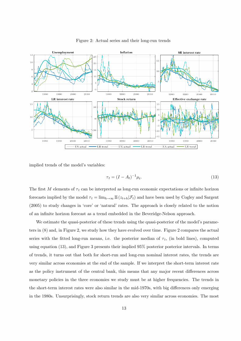
Figure 2: Actual series and their long-run trends
implied trends of the model�s variables:
� t = (I �At)�1�t: (13)
The �rst M elements of � t can be interpreted as long-run economic expectations or in�nite horizon
forecasts implied by the model � t = limh!1 E (zt+hjFt) and have been used by Cogley and Sargent
(2005) to study changes in �core�or �natural�rates. The approach is closely related to the notion
of an in�nite horizon forecast as a trend embedded in the Beveridge-Nelson approach.
We estimate the quasi-posterior of these trends using the quasi-posterior of the model�s parame-
ters in (8) and, in Figure 2, we study how they have evolved over time. Figure 2 compares the actual
series with the �tted long-run means, i.e. the posterior median of � t, (in bold lines), computed
using equation (13), and Figure 3 presents their implied 95% posterior posterior intervals. In terms
of trends, it turns out that both for short-run and long-run nominal interest rates, the trends are
very similar across economies at the end of the sample. If we interpret the short-term interest rate
as the policy instrument of the central bank, this means that any major recent di¤erences across
monetary policies in the three economies we study must be at higher frequencies. The trends in
the short-term interest rates were also similar in the mid-1970s, with big di¤erences only emerging
in the 1980s. Unsurprisingly, stock return trends are also very similar across economies. The most
13
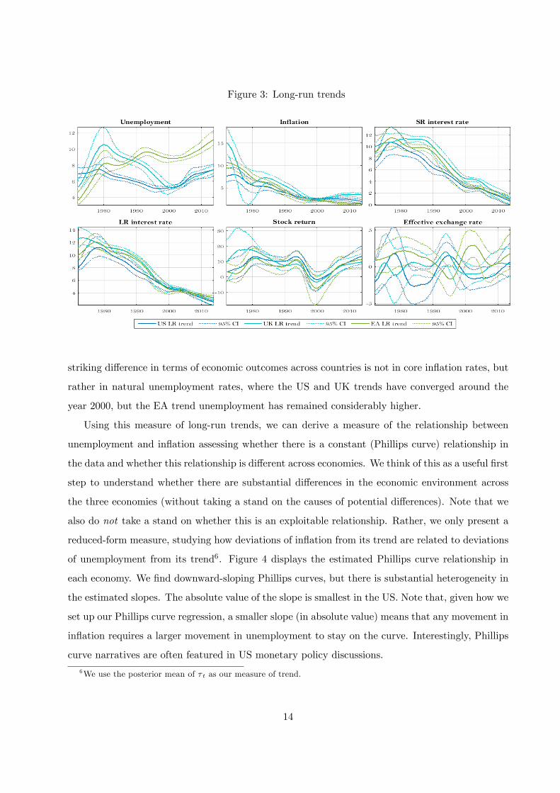
Figure 3: Long-run trends
striking di¤erence in terms of economic outcomes across countries is not in core in�ation rates, but
rather in natural unemployment rates, where the US and UK trends have converged around the
year 2000, but the EA trend unemployment has remained considerably higher.
Using this measure of long-run trends, we can derive a measure of the relationship between
unemployment and in�ation assessing whether there is a constant (Phillips curve) relationship in
the data and whether this relationship is di¤erent across economies. We think of this as a useful �rst
step to understand whether there are substantial di¤erences in the economic environment across
the three economies (without taking a stand on the causes of potential di¤erences). Note that we
also do not take a stand on whether this is an exploitable relationship. Rather, we only present a
reduced-form measure, studying how deviations of in�ation from its trend are related to deviations
of unemployment from its trend6. Figure 4 displays the estimated Phillips curve relationship in
each economy. We �nd downward-sloping Phillips curves, but there is substantial heterogeneity in
the estimated slopes. The absolute value of the slope is smallest in the US. Note that, given how we
set up our Phillips curve regression, a smaller slope (in absolute value) means that any movement in
in�ation requires a larger movement in unemployment to stay on the curve. Interestingly, Phillips
curve narratives are often featured in US monetary policy discussions.
6We use the posterior mean of � t as our measure of trend.
14
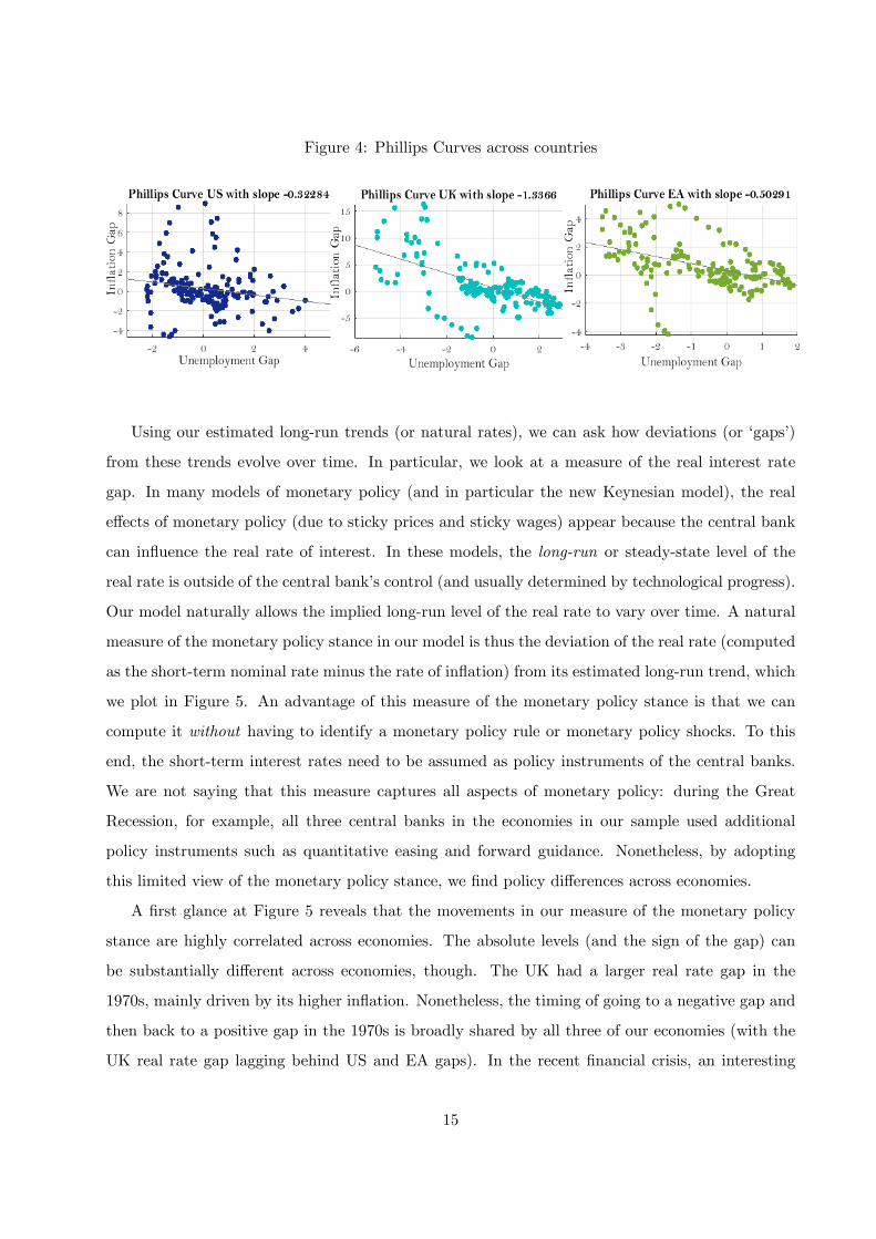
Figure 4: Phillips Curves across countries
Using our estimated long-run trends (or natural rates), we can ask how deviations (or �gaps�)
from these trends evolve over time. In particular, we look at a measure of the real interest rate
gap. In many models of monetary policy (and in particular the new Keynesian model), the real
e¤ects of monetary policy (due to sticky prices and sticky wages) appear because the central bank
can in�uence the real rate of interest. In these models, the long-run or steady-state level of the
real rate is outside of the central bank�s control (and usually determined by technological progress).
Our model naturally allows the implied long-run level of the real rate to vary over time. A natural
measure of the monetary policy stance in our model is thus the deviation of the real rate (computed
as the short-term nominal rate minus the rate of in�ation) from its estimated long-run trend, which
we plot in Figure 5. An advantage of this measure of the monetary policy stance is that we can
compute it without having to identify a monetary policy rule or monetary policy shocks. To this
end, the short-term interest rates need to be assumed as policy instruments of the central banks.
We are not saying that this measure captures all aspects of monetary policy: during the Great
Recession, for example, all three central banks in the economies in our sample used additional
policy instruments such as quantitative easing and forward guidance. Nonetheless, by adopting
this limited view of the monetary policy stance, we �nd policy di¤erences across economies.
A �rst glance at Figure 5 reveals that the movements in our measure of the monetary policy
stance are highly correlated across economies. The absolute levels (and the sign of the gap) can
be substantially di¤erent across economies, though. The UK had a larger real rate gap in the
1970s, mainly driven by its higher in�ation. Nonetheless, the timing of going to a negative gap and
then back to a positive gap in the 1970s is broadly shared by all three of our economies (with the
UK real rate gap lagging behind US and EA gaps). In the recent �nancial crisis, an interesting
15
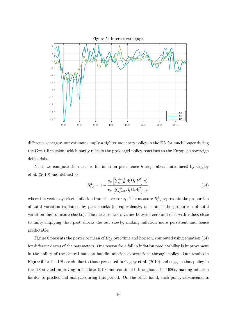
Figure 5: Interest rate gaps
di¤erence emerges: our estimates imply a tighter monetary policy in the EA for much longer during
the Great Recession, which partly re�ects the prolonged policy reactions to the European sovereign
debt crisis.
Next, we compute the measure for in�ation persistence h steps ahead introduced by Cogley
et al. (2010) and de�ned as
R2t;h = 1�e�
hPh�1j=0 A
jttA
j0t
ie0�
e�
hP1j=0A
jttA
j0t
ie0�
; (14)
where the vector e� selects in�ation from the vector zt. The measure R2t;h represents the proportion
of total variation explained by past shocks (or equivalently, one minus the proportion of total
variation due to future shocks). The measure takes values between zero and one, with values close
to unity implying that past shocks die out slowly, making in�ation more persistent and hence
predictable.
Figure 6 presents the posterior mean ofR2t;h over time and horizon, computed using equation (14)
for di¤erent draws of the parameters. One reason for a fall in in�ation predictability is improvement
in the ability of the central bank to handle in�ation expectations through policy. Our results in
Figure 6 for the US are similar to those presented in Cogley et al. (2010) and suggest that policy in
the US started improving in the late 1970s and continued throughout the 1980s, making in�ation
harder to predict and analyze during this period. On the other hand, such policy advancements
16
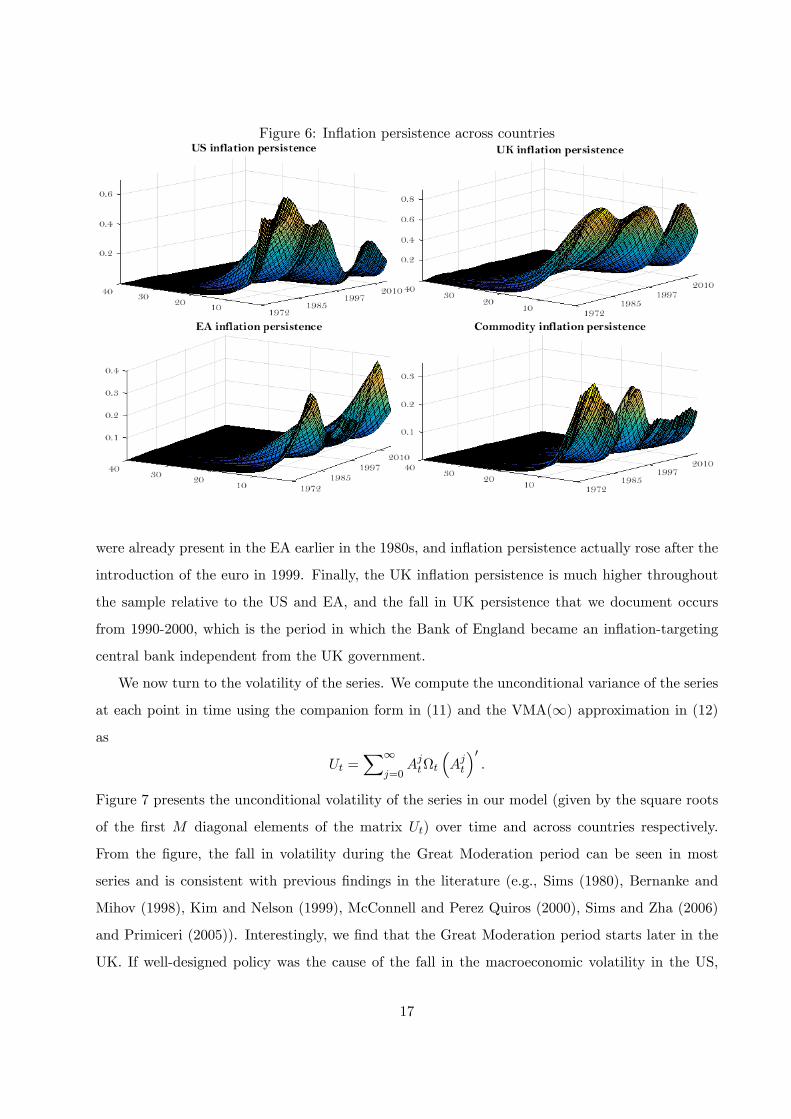
Figure 6: In�ation persistence across countries
were already present in the EA earlier in the 1980s, and in�ation persistence actually rose after the
introduction of the euro in 1999. Finally, the UK in�ation persistence is much higher throughout
the sample relative to the US and EA, and the fall in UK persistence that we document occurs
from 1990-2000, which is the period in which the Bank of England became an in�ation-targeting
central bank independent from the UK government.
We now turn to the volatility of the series. We compute the unconditional variance of the series
at each point in time using the companion form in (11) and the VMA(1) approximation in (12)
as
Ut =X1
j=0Ajtt
�Ajt
�0:
Figure 7 presents the unconditional volatility of the series in our model (given by the square roots
of the �rst M diagonal elements of the matrix Ut) over time and across countries respectively.
From the �gure, the fall in volatility during the Great Moderation period can be seen in most
series and is consistent with previous �ndings in the literature (e.g., Sims (1980), Bernanke and
Mihov (1998), Kim and Nelson (1999), McConnell and Perez Quiros (2000), Sims and Zha (2006)
and Primiceri (2005)). Interestingly, we �nd that the Great Moderation period starts later in the
UK. If well-designed policy was the cause of the fall in the macroeconomic volatility in the US,
17
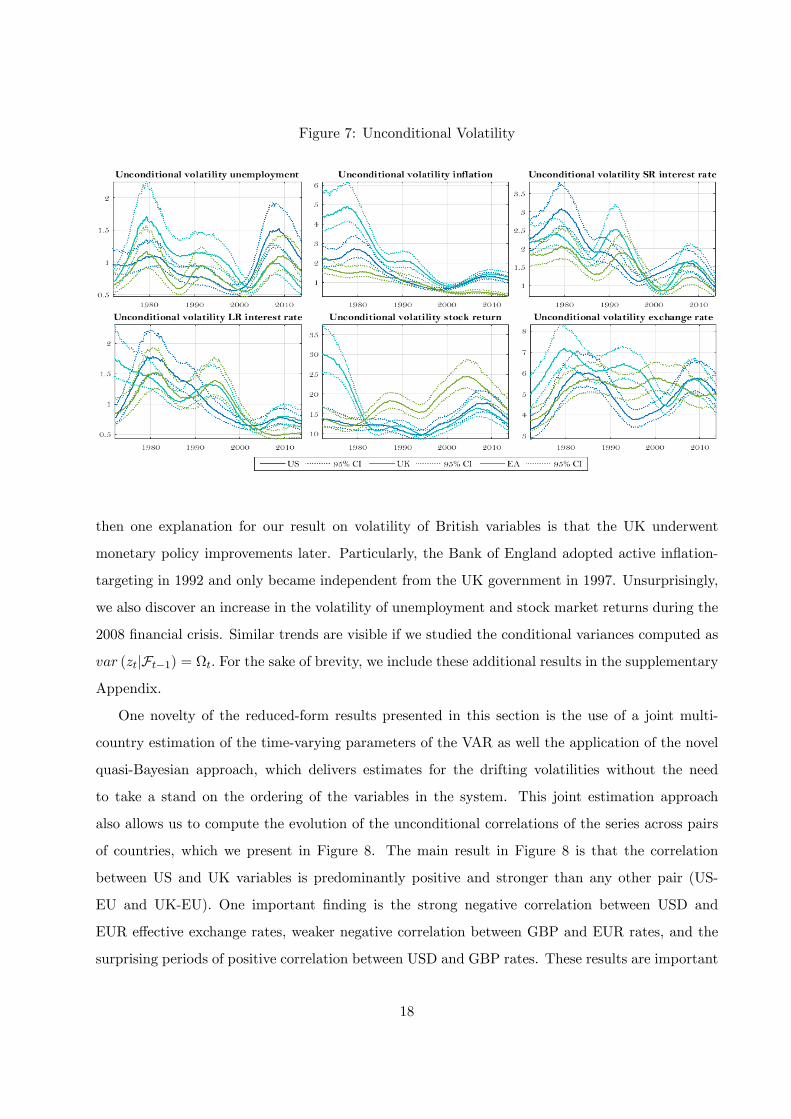
Figure 7: Unconditional Volatility
then one explanation for our result on volatility of British variables is that the UK underwent
monetary policy improvements later. Particularly, the Bank of England adopted active in�ation-
targeting in 1992 and only became independent from the UK government in 1997. Unsurprisingly,
we also discover an increase in the volatility of unemployment and stock market returns during the
2008 �nancial crisis. Similar trends are visible if we studied the conditional variances computed as
var (ztjFt�1) = t: For the sake of brevity, we include these additional results in the supplementary
Appendix.
One novelty of the reduced-form results presented in this section is the use of a joint multi-
country estimation of the time-varying parameters of the VAR as well the application of the novel
quasi-Bayesian approach, which delivers estimates for the drifting volatilities without the need
to take a stand on the ordering of the variables in the system. This joint estimation approach
also allows us to compute the evolution of the unconditional correlations of the series across pairs
of countries, which we present in Figure 8. The main result in Figure 8 is that the correlation
between US and UK variables is predominantly positive and stronger than any other pair (US-
EU and UK-EU). One important �nding is the strong negative correlation between USD and
EUR e¤ective exchange rates, weaker negative correlation between GBP and EUR rates, and the
surprising periods of positive correlation between USD and GBP rates. These results are important
18
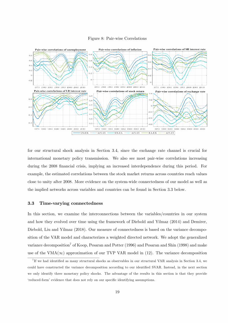
Figure 8: Pair-wise Correlations
for our structural shock analysis in Section 3.4, since the exchange rate channel is crucial for
international monetary policy transmission. We also see most pair-wise correlations increasing
during the 2008 �nancial crisis, implying an increased interdependence during this period. For
example, the estimated correlations between the stock market returns across countries reach values
close to unity after 2008. More evidence on the system-wide connectedness of our model as well as
the implied networks across variables and countries can be found in Section 3.3 below.
3.3 Time-varying connectedness
In this section, we examine the interconnections between the variables/countries in our system
and how they evolved over time using the framework of Diebold and Yilmaz (2014) and Demirer,
Diebold, Liu and Yilmaz (2018). Our measure of connectedness is based on the variance decompo-
sition of the VAR model and characterizes a weighted directed network. We adopt the generalized
variance decomposition7 of Koop, Pesaran and Potter (1996) and Pesaran and Shin (1998) and make
use of the VMA(1) approximation of our TVP VAR model in (12). The variance decomposition7 If we had identi�ed as many structural shocks as observables in our structural VAR analysis in Section 3.4, we
could have constructed the variance decomposition according to our identi�ed SVAR. Instead, in the next section
we only identify three monetary policy shocks. The advantage of the results in this section is that they provide
�reduced-form�evidence that does not rely on our speci�c identifying assumptions.
19
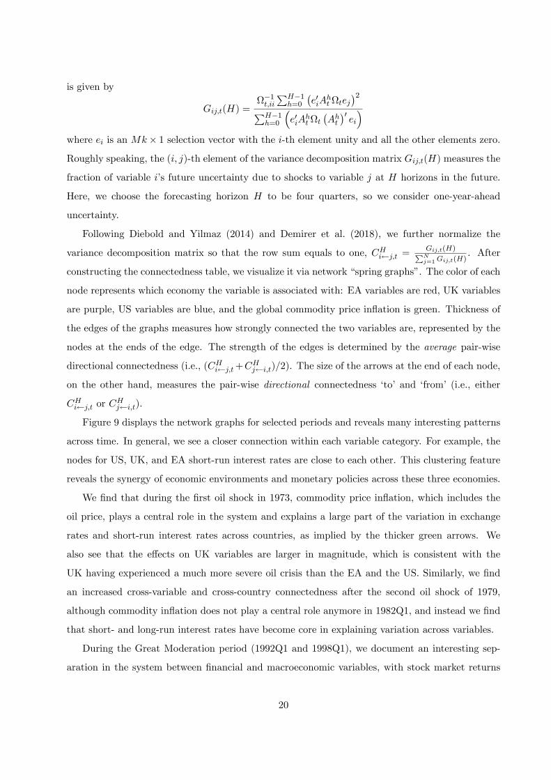
is given by
Gij;t(H) =�1t;ii
PH�1h=0
�e0iA
httej
�2PH�1h=0
�e0iA
htt
�Aht�0ei
�where ei is an Mk� 1 selection vector with the i-th element unity and all the other elements zero.
Roughly speaking, the (i; j)-th element of the variance decomposition matrix Gij;t(H) measures the
fraction of variable i�s future uncertainty due to shocks to variable j at H horizons in the future.
Here, we choose the forecasting horizon H to be four quarters, so we consider one-year-ahead
uncertainty.
Following Diebold and Yilmaz (2014) and Demirer et al. (2018), we further normalize the
variance decomposition matrix so that the row sum equals to one, CHi j;t =Gij;t(H)PNj=1Gij;t(H)
. After
constructing the connectedness table, we visualize it via network �spring graphs�. The color of each
node represents which economy the variable is associated with: EA variables are red, UK variables
are purple, US variables are blue, and the global commodity price in�ation is green. Thickness of
the edges of the graphs measures how strongly connected the two variables are, represented by the
nodes at the ends of the edge. The strength of the edges is determined by the average pair-wise
directional connectedness (i.e., (CHi j;t+CHj i;t)=2). The size of the arrows at the end of each node,
on the other hand, measures the pair-wise directional connectedness �to� and �from� (i.e., either
CHi j;t or CHj i;t).
Figure 9 displays the network graphs for selected periods and reveals many interesting patterns
across time. In general, we see a closer connection within each variable category. For example, the
nodes for US, UK, and EA short-run interest rates are close to each other. This clustering feature
reveals the synergy of economic environments and monetary policies across these three economies.
We �nd that during the �rst oil shock in 1973, commodity price in�ation, which includes the
oil price, plays a central role in the system and explains a large part of the variation in exchange
rates and short-run interest rates across countries, as implied by the thicker green arrows. We
also see that the e¤ects on UK variables are larger in magnitude, which is consistent with the
UK having experienced a much more severe oil crisis than the EA and the US. Similarly, we �nd
an increased cross-variable and cross-country connectedness after the second oil shock of 1979,
although commodity in�ation does not play a central role anymore in 1982Q1, and instead we �nd
that short- and long-run interest rates have become core in explaining variation across variables.
During the Great Moderation period (1992Q1 and 1998Q1), we document an interesting sep-
aration in the system between �nancial and macroeconomic variables, with stock market returns
20
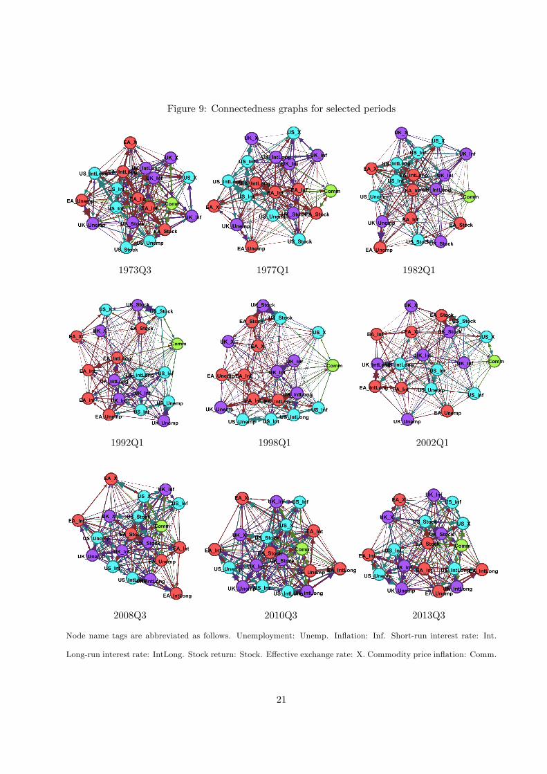
Figure 9: Connectedness graphs for selected periods
1973Q3 1977Q1 1982Q1
1992Q1 1998Q1 2002Q1
2008Q3 2010Q3 2013Q3
Node name tags are abbreviated as follows. Unemployment: Unemp. In�ation: Inf. Short-run interest rate: Int.
Long-run interest rate: IntLong. Stock return: Stock. E¤ective exchange rate: X. Commodity price in�ation: Comm.
21
and exchange rates of our three economies forming a cluster, implying not much spillover e¤ects be-
tween �nancial markets and the macroeconomy. During these periods, we �nd that UK short- and
long-run interest rates are strongly connected to UK in�ation with large portions of the variation
in in�ation explained by the rates and vice versa, a possible consequence of the introduction of in-
�ation targeting and its formal independence from the government in 1992 and 1997, respectively.
In 2002Q1, after the short 2001 NBER recession, we continue to �nd some separation between
�nancial and macro variables, although less clear than in the previous periods.
During the 2008 crisis and the periods afterward, we uncover an increased global interdepen-
dence (implied by the thicker arrows) and importantly, we �nd that stock returns are now central
in the estimated network, implying large contagion from �nancial markets to the macroeconomy.
Particularly, stock returns are directly explaining large proportions of the variation in unemploy-
ment, in�ation, and interest rates across countries. Our results are very similar in 2010Q3, with
commodity price in�ation now also playing a central role in the system.
The graphs presented so far try to uncover relationships between di¤erent variables in our
model. We can also use the information in those graphs to get a sense of how important unexpected
movements in other variables are on average in our system over time. This gives us an estimate of
how important interdependence or the �network structure�is in our data and, in particular, how it
has evolved over time. To achieve this goal, we measure the interaction across variables net of the
self e¤ect by averaging over the connectedness table excluding the diagonal elements,
CHt =1
N
XN
i;j=1;i6=jCHi j;t:
Figure 10 presents the posterior median and the 64% estimated posterior sets of our system-wide
connectedness measure, evolving over time, and the shaded grey top, middle, and bottom areas
display recession dates in the US, UK, and EA, respectively8. In general, Figure 10 suggests
that periods characterized by economic downturns (such as the Great In�ation in the early 1970s,
the EA and UK recessions around the middle 1990s, as well as the �nancial crisis, the Great
Recession, and the European sovereign debt crisis in the late 2000s) are associated with higher
overall connectedness. Particularly, over 80% of the variance of our model is explained by past
shocks to other variables during the recent crisis, compared to 60% in the Great Moderation. This
result suggests that during economic distress, correlations and interdependencies between variables8For the US, we use NBER recession dates; for the UK and EA, we use an OECD monthly recession indicators
from peak through trough and de�ne a recession in the UK and EA as �ve consecutive months of decline in each,
respectively.
22
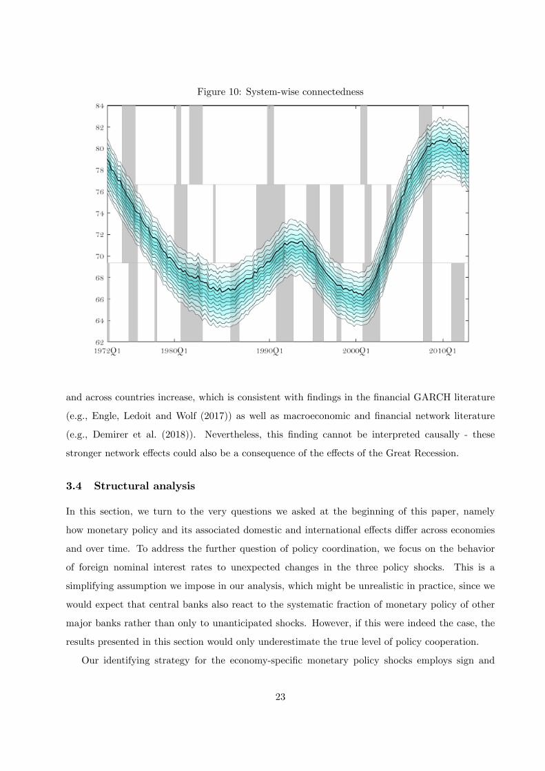
Figure 10: System-wise connectedness
and across countries increase, which is consistent with �ndings in the �nancial GARCH literature
(e.g., Engle, Ledoit and Wolf (2017)) as well as macroeconomic and �nancial network literature
(e.g., Demirer et al. (2018)). Nevertheless, this �nding cannot be interpreted causally - these
stronger network e¤ects could also be a consequence of the e¤ects of the Great Recession.
3.4 Structural analysis
In this section, we turn to the very questions we asked at the beginning of this paper, namely
how monetary policy and its associated domestic and international e¤ects di¤er across economies
and over time. To address the further question of policy coordination, we focus on the behavior
of foreign nominal interest rates to unexpected changes in the three policy shocks. This is a
simplifying assumption we impose in our analysis, which might be unrealistic in practice, since we
would expect that central banks also react to the systematic fraction of monetary policy of other
major banks rather than only to unanticipated shocks. However, if this were indeed the case, the
results presented in this section would only underestimate the true level of policy cooperation.
Our identifying strategy for the economy-speci�c monetary policy shocks employs sign and
23
magnitude restrictions of the impulse responses, along the lines of Uhlig (2005), Canova and Nicolo
(2002), and Faust (1998). Speci�cally, we impose the sign restrictions that in response to a monetary
policy shock in country i, the short-term nominal rate in that country increases, the in�ation rate
decreases, and the unemployment rate increases. Moreover, to distinguish monetary policy shocks
across countries, we also impose that a monetary policy shock in country i must have the largest
e¤ect in magnitude on in�ation, unemployment, and interest rate in country i. These magnitude
restrictions can be powerful tools that help shrink the identi�ed set of impulse responses, as carefully
detailed in Amir-Ahmadi and Drautzburg (2017).
More formally, we use the VMA(1) approximation of the companion model in (12) and let Ptdenote the Cholesky factor of ��1t : To impose our identifying restrictions, for each period t, we �rst
draw from a family of orthogonal matrices Q 2 Q of size M , and the resulting impulse responses
at every point in time, given by �th = [Ajt ]1:M;1:MPtQ0; span the space of all possible responses9.
Next, we employ rejection sampling, only retaining draws of �th that satisfy all sign and magnitude
restrictions. Namely, we check if a shock can be found for each economy i 2 f1; 2; 3g satisfying the
following: an increase in domestic interest rate (rit0 > 0) reduces on impact (i.e., h = 0) domestic
in�ation (�it0 � 0), increases domestic unemployment (uit0 � 0), and, in addition, the shock has the
highest magnitude e¤ect on the three domestic variables:���rit0�� > ����rjt0��� ; ����it0�� > �����jt0��� and���uit0�� > ����ujt0��� for all j 6= i: To implement the calculation of the impulse responses conditional
on reduced-form estimates, we use the algorithm outlined in Rubio-Ramirez, Waggoner and Zha
(2010), which allows us to e¢ ciently explore the space of candidate impulse responses. Notice that
we leave unrestricted the direction in which a policy shock in a given country might a¤ect the
remaining domestic variables (long-run interest rates, exchange rates, and stock returns) as well
as all foreign variables. As a consequence, the results on the size and direction of the spillover
e¤ects of shocks across countries are informed by the data only and not imposed as a maintained
assumption. In the main text, we focus on the point-wise impulse responses (computed as the
posterior mean) to a one standard deviation shock for selected time periods. The supplementary
Appendix contains both the associated posterior error bands as well as 3D plots that display the
entire evolution of the posterior mean responses. For the sake of clarity, throughout this section
and the Appendix, we always use dark blue for the US policy shocks, lighter blue for UK shocks,
and green for EA shocks.
In Figure 11, we show the responses of all domestic variables to a monetary policy shock in
9Note that we draw di¤erent Qs for di¤erent periods. [�]1:M;1:M selects the �rst M �M block of a given matrix.
24
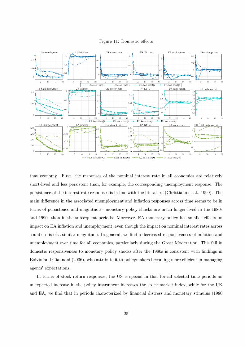
Figure 11: Domestic e¤ects
that economy. First, the responses of the nominal interest rate in all economies are relatively
short-lived and less persistent than, for example, the corresponding unemployment response. The
persistence of the interest rate responses is in line with the literature (Christiano et al., 1999). The
main di¤erence in the associated unemployment and in�ation responses across time seems to be in
terms of persistence and magnitude - monetary policy shocks are much longer-lived in the 1980s
and 1990s than in the subsequent periods. Moreover, EA monetary policy has smaller e¤ects on
impact on EA in�ation and unemployment, even though the impact on nominal interest rates across
countries is of a similar magnitude. In general, we �nd a decreased responsiveness of in�ation and
unemployment over time for all economies, particularly during the Great Moderation. This fall in
domestic responsiveness to monetary policy shocks after the 1980s is consistent with �ndings in
Boivin and Giannoni (2006), who attribute it to policymakers becoming more e¢ cient in managing
agents�expectations.
In terms of stock return responses, the US is special in that for all selected time periods an
unexpected increase in the policy instrument increases the stock market index, while for the UK
and EA, we �nd that in periods characterized by �nancial distress and monetary stimulus (1980
25
and 2010) the responses are negative, suggesting asymmetry in the responses of �nancial markets to
policy shocks. Finally, exchange rates mostly move in the expected direction: monetary tightening
causes an appreciation in the e¤ective exchange rate. One exception is the UK, as well as the EA
in periods before the introduction of the euro. This is expected, as the UK and the aggregated
individual European states prior to 1999 resemble more closely small open economies that have less
control over the value of their currencies in international markets.
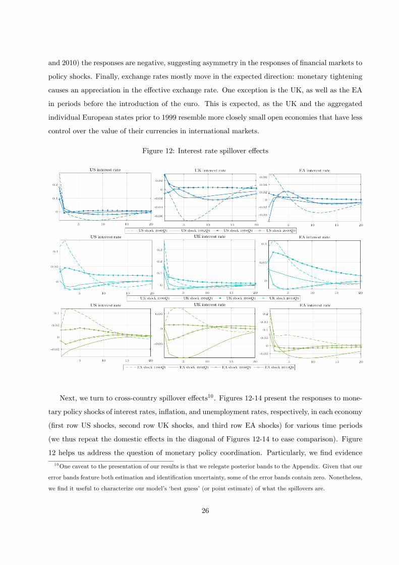
Figure 12: Interest rate spillover e¤ects
Next, we turn to cross-country spillover e¤ects10. Figures 12-14 present the responses to mone-
tary policy shocks of interest rates, in�ation, and unemployment rates, respectively, in each economy
(�rst row US shocks, second row UK shocks, and third row EA shocks) for various time periods
(we thus repeat the domestic e¤ects in the diagonal of Figures 12-14 to ease comparison). Figure
12 helps us address the question of monetary policy coordination. Particularly, we �nd evidence
10One caveat to the presentation of our results is that we relegate posterior bands to the Appendix. Given that our
error bands feature both estimation and identi�cation uncertainty, some of the error bands contain zero. Nonetheless,
we �nd it useful to characterize our model�s �best guess�(or point estimate) of what the spillovers are.
26
of policy coordination only during the 1970s and early 1980s, and zero or negative cooperation
afterwards. To put this result into historical context, the 1970s and 1980s were periods when
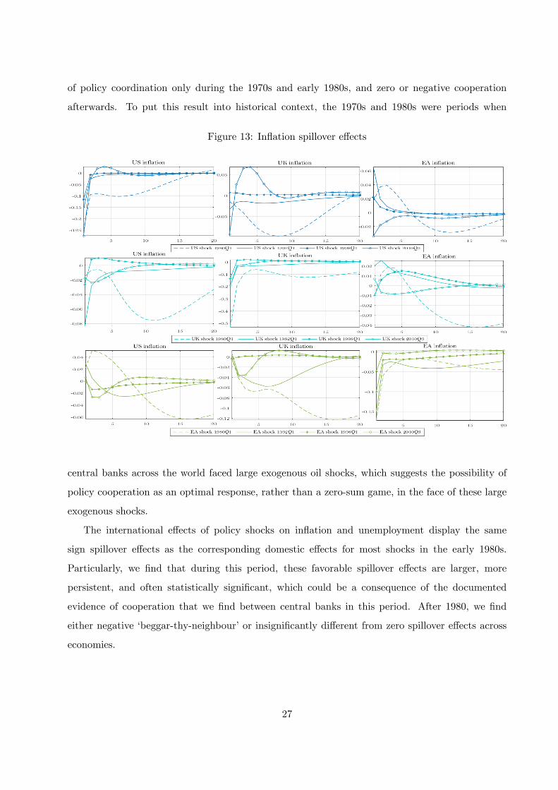
Figure 13: In�ation spillover e¤ects
central banks across the world faced large exogenous oil shocks, which suggests the possibility of
policy cooperation as an optimal response, rather than a zero-sum game, in the face of these large
exogenous shocks.
The international e¤ects of policy shocks on in�ation and unemployment display the same
sign spillover e¤ects as the corresponding domestic e¤ects for most shocks in the early 1980s.
Particularly, we �nd that during this period, these favorable spillover e¤ects are larger, more
persistent, and often statistically signi�cant, which could be a consequence of the documented
evidence of cooperation that we �nd between central banks in this period. After 1980, we �nd
either negative �beggar-thy-neighbour�or insigni�cantly di¤erent from zero spillover e¤ects across
economies.
27
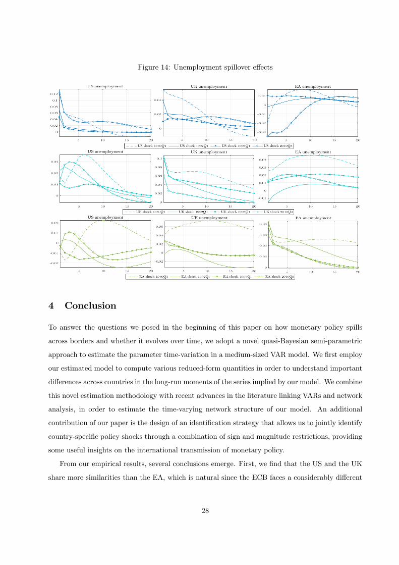
Figure 14: Unemployment spillover e¤ects
4 Conclusion
To answer the questions we posed in the beginning of this paper on how monetary policy spills
across borders and whether it evolves over time, we adopt a novel quasi-Bayesian semi-parametric
approach to estimate the parameter time-variation in a medium-sized VAR model. We �rst employ
our estimated model to compute various reduced-form quantities in order to understand important
di¤erences across countries in the long-run moments of the series implied by our model. We combine
this novel estimation methodology with recent advances in the literature linking VARs and network
analysis, in order to estimate the time-varying network structure of our model. An additional
contribution of our paper is the design of an identi�cation strategy that allows us to jointly identify
country-speci�c policy shocks through a combination of sign and magnitude restrictions, providing
some useful insights on the international transmission of monetary policy.
From our empirical results, several conclusions emerge. First, we �nd that the US and the UK
share more similarities than the EA, which is natural since the ECB faces a considerably di¤erent
28
environment as the policymaker of a currency union comprised of diverse member states. This
is particularly evident in our measure of the monetary policy stance as well as in the domestic
responses to monetary policy shocks. Our reduced-form analysis also points to some meaningful
changes in the UK monetary policy after the Bank of England underwent structural changes in the
1990s. Second, we uncover an increased connectedness between the variables in our model during
the recent �nancial crisis, and more generally, in periods with �nancial distress. While we �nd this
result compelling, we are cautious to conjecture on whether increased connectedness is the cause
or merely a symptom of recessions. Finally, our structural shock analysis suggests that monetary
policy shocks were larger in magnitude and more persistent in all countries in the early 1980s than
in any subsequent periods. In the same period, we also �nd evidence for positive spillover e¤ects of
policy between countries as well as policy coordination between the three central banks analyzed.
References
Alesina, A., Blanchard, O., Gali, J., Giavazzi, F. and Uhlig, H. (2001). De�ning a Macroeconomic Framework for
The Euro Area: Montiroing the EUropen Central Bank 3, CEPR.
Amir-Ahmadi, P. and Drautzburg, T. (2017). Identi�cation Through Heterogeneity, Working Papers 17-11, Federal
Reserve Bank of Philadelphia.
Amir-Ahmadi, P., Matthes, C. and Wang, M. (2016). Drifts and volatilities under measurement error: Assessing
monetary policy shocks over the last century, Quantitative Economics 7(2): 591�611.
Amisano, G., Giannone, D. and Lenza, M. (2015). Large time varying parameter VARs for macroeconomic forecasting,
Working paper .
Banbura, M., Giannone, D. and Reichlin, L. (2010). Large Bayesian vector autoregressions, Journal of Applied
Econometrics 25(1): 71�92.
Benigno, G. and Benigno, P. (2006). Designing targeting rules for international monetary policy cooperation, Journal
of Monetary Economics 53(3): 473�506.
Bernanke, B. and Mihov, I. (1998). Measuring monetary policy, Quarterly Journal of Economics 113: 869�902.
Beyer, A., Gaspar, V., Gerberding, C. and Issing, O. (2008). Opting Out of the Great In�ation: German Monetary
Policy After the Break Down of Bretton Woods, NBER Working Papers 14596, National Bureau of Economic
Research, Inc.
Billio, M., Casarin, R., Ravazzolo, F. and Van Dijk, H. K. (2016). Interconnections Between Eurozone and US
Booms and Busts Using a Bayesian Panel Markov-Switching VAR Model, Journal of Applied Econometrics
31(7): 1352�1370.
Bognanni, M. (2018). A class of time-varying parameter structural vars for inference under exact or set identi�cation,
Technical report, Federal Reserve Bank of Cleveland.
29
Boivin, J. and Giannoni, M. (2006). Has monetary policy become more e¤ective?, Review of Economics and Statistics
88(3): 445�462.
Canova, F. and Ciccarelli, M. (2009). Estimating Multicountry Var Models, International Economic Review
50(3): 929�959.
Canova, F., Ciccarelli, M. and Ortega, E. (2007). Similarities and convergence in G-7 cycles, Journal of Monetary
Economics 54(3): 850�878.
Canova, F. and Nicolo, G. D. (2002). Monetary disturbances matter for business �uctuations in the g-7, Journal of
Monetary Economics 49(6): 1131�1159.
Canova, F. and Sala, L. (2009). Back to square one: Identifcation issues in DSGE models, Journal of Monetary
Economics 56(4): 431�449.
Canzoneri, M. and Gray, J. A. (1985). Monetary policy games and the consequences of non-cooperative behavior,
International economic review 25(3): 547�564.
Christiano, L., Eichenbaum, M. and Evans, C. (1999). Monetary policy shocks: What have we learned and to what
end?, in J. B. Taylor and M. Woodford (eds), Handbook of Macroeconomics, Vol. 1A, Elsevier, pp. 65�148.
Clarida, R., Gali, J. and Gertler, M. (2002). A simple framework for international monetary policy analysis, Journal
of monetary economics 49: 879�904.
Clark, T. E. (2012). Real-time density forecasting from BVARs with stochastic volatility, Journal of Business and
Economic Statistics 29(3): 327�341.
Coenen, G., Lombardo, G., Smets, F. and Straub, R. (2007). International transmission and monetary policy
cooperation, International Dimensions of monetary policy, University of Chicago Press, pp. 157�192.
Cogley, T., Primiceri, G. E. and Sargent, T. J. (2010). In�ation-gap persistence in the US, American Economic
Journal: Macroeconomics 2(1): 43�69.
Cogley, T. and Sargent, T. J. (2005). Drifts and volatilities: Monetary policies and outcomes in the post World War
II US, Review of Economic Dynamics 8: 262�302.
Corsetti, G. and Pesenti, P. (2001). Welfare and macroeconomic interdependence*, The Quarterly Journal of Eco-
nomics 116(2): 421�445.
Corsetti, G. and Pesenti, P. (2005). International dimensions of optimal monetary policy, Journal of Monetary
Economics 52(2): 281�305.
De Graeve, F. and Karas, A. (2010). Identifying VARs through Heterogeneity: An Application to Bank Runs,
Working paper series, Sveriges Riksbank (Central Bank of Sweden).
Demirer, M., Diebold, F. X., Liu, L. and Yilmaz, K. (2018). Estimating global bank network connectedness, Journal
of Applied Econometrics 33(1): 1�15.
di Giovanni, J., McCrary, J. and von Wachter, T. (2009). Following Germany�s Lead: Using International Monetary
Linkages to Estimate the E¤ect of Monetary Policy on the Economy, The Review of Economics and Statistics
91(2): 315�331.
30
DiCecio, R. and Nelson, E. (2009). The Great In�ation in the United States and the United Kingdom: Reconciling
Policy Decisions and Data Outcomes, Nber working papers, National Bureau of Economic Research, Inc.
Diebold, F. and Yilmaz, K. (2014). On the network topology of variance decompositions: Measuring the connectedness
of �nancial �rms, Journal of Econometrics 182: 119�134.
Engle, R., Ledoit, O. and Wolf, M. (2017). Large dynamic covariance matrices, Journal of Bussiness and Economic
Statistics .
Fagan, G., Henry, J. and Mestre, R. (2001). An area-wide model (AWM) for the euro area, Working paper series,
European Central Bank.
Faust, J. (1998). The robustness of identi�ed VAR conclusions about money, Carnegie-Rochester Conference Series
on Public Policy 49: 207�244.
Gali, J. and Monacelli, T. (2005). Monetary policy and exchange rate volatility in a small open economy, Review of
economic studies 72: 707�734.
Gerko, E. and Rey, H. (2017). Monetary Policy in the Capitals of Capital, Nber working papers, National Bureau of
Economic Research, Inc.
Giraitis, L., Kapetanios, G. and Yates, T. (2014). Inference on stochastic time-varying coe¢ cient models, Journal of
Econometrics 179(1): 46�65.
Giraitis, L., Kapetanios, G. and Yates, T. (2018). Inference on multivariate heteroscedastic time varying random
coe¢ cient models, Journal of Time Series Analysis 39(2): 129�149.
Kadiyala, K. R. and Karlsson, S. (1997). Numerical methods for estimation and inference in Bayesian VAR models,
Journal of Applied Econometrics 12(2): 99�132.
Kilian, L. and Luetkepohl, H. (2017). Structural Vector Autoregressive Analysis, Cambridge University Press.
Kim, C. and Nelson, C. R. (1999). Has the U.S. Economy become more stable? A Bayesian Approach based on a
Markov-Switching Model of the Business Cycle, Review of Economics and Statistics 81(4): 608�618.
Koop, G. and Korobilis, D. (2018). Forecasting with high-dimensional panel VARs, Essex Finance Centre Working
Papers 21329, University of Essex, Essex Business School .
Koop, G., Pesaran, M. and Potter, S. (1996). Impulse Response Analysis in Nonlinear Multivariate Models, Journal
of Econometrics 74(1): 119�147.
Lubik, T. and Schorfheide, F. (2006). A Bayesian Look at the New Open Economy Macroeconomics, NBER Macro-
economics Annual 2005, Volume 20, NBER Chapters, National Bureau of Economic Research, Inc, pp. 313�382.
McConnell, M. and Perez Quiros, G. (2000). Output �uctuations in the U.S.: what has changed since the early
1980s?, American Economic Review 90: 1464�1476.
Mumtaz, H. and Surico, P. (2009). Time-varying yield curve dynamics and monetary policy, Journal of Applied
Econometrics 24(6): 895�913.
Mundell, R. A. (1963). Capital mobility and stabilization policy under �xed and �exible exchange rates, Canadian
Journal of Economics and Political Science 29.
Obstfeld, M. and Rogo¤, K. (1995). Exchange rate dynamics redux, Journal of political economy 103(3): 624�660.
31
Pesaran, H. and Shin, Y. (1998). Generalized Impulse Response Analysis in Linear Multivariate Models, Economics
Letters 58(1): 17�29.
Petrova, K. (2018). A quasi-bayesian local likelihood approach to time varying parameter VAR models, Journal of
Econometrics, Forthcoming .
Primiceri, G. (2005). Time-varying structural vector autoregressions and monetary policy, Review of Economic
Studies 72(3): 821�852.
Rubio-Ramirez, J. F., Waggoner, D. F. and Zha, T. (2010). Structural Vector Autoregressions: Theory of Identi�ca-
tion and Algorithms for Inference, Review of Economic Studies 77(2): 665�696.
Sims, C. A. (1980). Macroeconomics and reality, Econometrica 48: 1�48.
Sims, C. A. and Zha, T. (2006). Were there regime switches in U.S. monetary policy?, American Economic Review
96: 1193�1224.
Stephane, D., Pesaran, H., Smith, V. and Smith, R. (2013). Constructing multi-country rational expectations models,
Oxford Bulletin of Economics and Statistics 76(6): 812�840.
Uhlig, H. (2005). What are the e¤ects of monetary policy on output? results from an agnostic identi�cation procedure,
Journal of Monetary Economics 52(2): 381�419.
32