DOC #127919 v7 1

Monitoring Small Area Growth with GIS:

An Application to the City of Los Angeles

Simon Choi*, Ping Wang, Elizabeth Delgado, Sung Ho Ryu

Southern California Association of Governments

818 West 7th Street 12th Floor

Los Angeles, CA 90017

* choi@scag.ca.gov

* 213-236-1849

&

Kyuyoung Cho

Department of Urban Information Engineering,

Anyang University, South Korea

kyuyoung@anyang.ac.kr

Paper presented at the 2007 ESRI International User Conference,

San Diego, California, June 18-22, 2007

DOC #127919 v7 2

Abstract

This paper presents a technique of monitoring small area growth with GIS.

Monitoring growth of small areas, including census tracts, blocks, or traffic analysis

zones, becomes an important tool in measuring changes in small area plans (e.g.,

transit oriented development). Although geo-coded databases have become more

popular and easily accessible in recent days, most available data is still spatially

aggregated. The raster cell can be developed as a spatial base unit for monitoring

small area growth. Spatially aggregated small area data is disaggregated into raster

cells using land use information from both aerial photographs and local general

plans. This study uses the land use weighted interpolation to develop uneven and

hopefully more accurate distribution of the socioeconomic estimates within the census

tract of the City of Los Angeles. This paper also discusses how to monitor the

changing size and spatial distribution of small area household growth, specifically in

and around the transit oriented development (TOD) areas. ArcGIS Spatial Analyst is

used to implement the raster cell method.

1. Introduction

Urban and regional planning requires a variety of socioeconomic data at the small

area level to do detailed analysis. The socioeconomic estimates at the small area play

an important role in tracing the recent trends and figuring out the likely growth pattern

of the small area. Those estimates are useful to assess the effectiveness of the policy

and programs, or to evaluate the accuracy of the small area growth forecasts. Small

area analysis is made possible with the effective use of the geographic information

system (GIS).

The small area is not defined in a definite way, but in relative way (Smith and

Morrison, 2005). Demographers might treat a county as a small area, the regional

scientist might treat a metropolitan region as a small area, and transportation planner

might a transportation analysis zone as a small area. The U.S. Census Bureau

publishes socioeconomic data for a variety of small statistical areas. Even a census

block, the smallest size of U.S. Census statistical area, would be able to contain

necessary socioeconomic data.

The nature of the available socioeconomic data for those small size statistical areas is

spatially aggregated in a way that the socioeconomic data is difficult to be used for the

very small area analysis needed. For example, we might be interested in knowing the

number of housing units within a certain distance (e.g., 1/4 miles or 1/3 miles) of the

transit station/corridor, the number of jobs available within 30 minutes of the

residence area, the number of low income household within a certain distance of the

freeway, the number of residents living within a certain distance of the hazardous

toxic facility or even how these variables change over time. How do we process

socioeconomic data relevant to a specific very small area?

The area interpolation method plays a key role in determining the socioeconomic

estimates of the small area. Area weighting have been widely used due to its easy

applicability. This method, however, might not produce the accurate socioeconomic

estimates because of its “even distribution” assumption. This study uses the land use

DOC #127919 v7 3

weighted interpolation method to reflect uneven, and hopefully more accurate,

distribution of the socioeconomic estimates within the small area. As a base

geographical unit, the raster cell is an easily modifiable small size zone. The raster

cell level socioeconomic data estimates can be easily derived because of easy access

to land use image data from aerial photographs. Further, the study illustrates how

socioeconomic data at the raster cell level would be used to monitor the changing size

and spatial distribution of small area housing growth, particularly, in and around

transit oriented development areas.

2. Raster Cell Methods for Small Area Estimates and Forecasts

2-1. Process of developing small area growth estimates and forecasts

The development of the small area growth forecast involves several steps (SCAG,

2007).1 The following process is based on the recent growth estimates and forecast

experience of the Southern California Association of Government (SCAG):

1) The first step starts with an analysis of recent regional growth trends and the

collection of significant local general plan updates. A variety of large area

estimates and projections are collected from diverse federal, state, and local data

sources.

2) The second step involves the review and update of the existing regional growth

forecast methodology and key assumptions. The widely used methodology

includes the cohort-component method and the shift-share method. The key

technical assumptions included updates regarding the fertility rate, mortality rate,

net immigration, domestic in-migration, domestic out-migration, labor force

participation rates, double jobbing rates, unemployment rates, and headship rates,

etc.

3) The third step is to review, update and assess existing regional growth policies

and strategies, including land use strategies, economic growth initiatives and

goods movement strategies. Relevant analysis also includes general plan capacity

analysis, application of SCAG’s Compass Blueprint Program demonstration

projects, regional growth principles, polling and focus groups, and public

workshops.

4) The fourth step is to develop and evaluate the draft regional growth forecast

scenarios with small area distributions. Regional growth forecast scenarios are

developed and allocated into the smaller geographic levels using public

workshops. The small area distributions of the regional growth are evaluated

using transportation and emission modeling results and environmental impact

review (EIR) reports.

5) The fifth and last step is to select and adopt a preferred regional growth forecast.

A regional growth scenario with selected small area distributions is developed

1 (http://scag.ca.gov/Housing/pdfs/rhna/RHNA_Methodology_rc020107.pdf)

DOC #127919 v7 4

using transportation and environmental performance measures. A regional growth

forecast is adopted by the SCAG Regional Council.

An organized forecasting decision making process is required to develop a consensus

regional growth forecast in an efficient, open, and fair way. A variety of groups and

input is involved in the forecasting process include panel of experts, subregional/local

review, stakeholders/data users, public outreach, technical committee, policy

committee, and the SCAG Regional Council.

Using the Southern California six county region2 as an example, the household

forecasts are developed at different levels of geography (see figure 1). The raster cell

is currently not identified as an official geographic unit, but is being introduced for

this study.

Figure 1. Different levels of geography for household forecasts

2-2. Raster Cell Methods

2 Southern California Six County Region includes the following six counties: Imperial, Los Angeles,

Orange, Riverside, San Bernardino, and Ventura. There are 187 cities in the 38,000 square mile region.

The region’s current population is 18 million or more, accounting for more than 6% of the U.S national

population, and approximately half of the California population.

City/Unincorporated

Areas

Raster Cell

Partial Census Tract

(PT)

PT / TAZ

County

Census Tract (CT)

Traffic Analysis Zone

(TAZ)

Region

DOC #127919 v7 5

The spatially aggregated socioeconomic data at the census tract level can be easily

disaggregated into any small size zone using the area interpolation. The GIS analysis

does not require developing a raster cell as a spatial unit base. The more accurate

socioeconomic information at the smaller area level (e.g., raster cell), however, is

expected to inform public policy, or to support business decision making (Smith and

Morrison, 2005).

GIS interpolation techniques are used to (whole or percentage) disaggregate the CT

level households for buffer analysis related to TOD. Analysis of the growth within a

certain distance of the station can be done using the method above.

The small area socioeconomic data of the U.S. Census can be easily summed to the

large area socioeconomic data in many cases. The major problem occurs when the

spatial analysis is needed for newly identified small areas, such as transportation

analysis zones or neighborhood areas within a quarter mile distance of the train

stations/ bus stops. Any other interpolation technique might not accurately depict the

socioeconomic characteristics because of the data conversion process.

A better approach would be to use socioeconomic data of the smallest zone, which

could be based on a “geo-coded” parcel (Mouden and Hubner, 2000). The tax-lot

parcel becomes an important unit of land information, data collection and analysis

(Enger 1992; Bollens, 1998). For example, we might be able to estimate the number

of births and deaths for any different size of small area, if the birth or death data is

available in a “geo-coded” parcel format. The Center for Demographic Research

(CDR), California State University, Fullerton, annually estimates natural increase of

the small areas of the County of Orange. Geo-coded parcel data is the ideal unit of

analysis and has become more useful and popular in recent days, but such data is

expensive, hardly accessible, and limited in its scope.

The tax-lot parcel contains the following land and building characteristics: acreage,

land use, land value, improvement value, housing units, square footage, year built,

bedrooms/bathrooms, amongst other factors. This information is conveniently

available to the general public. For example, Los Angeles County Office of the

Assessor developed the Property Assessment Information System (PAIS) to enhance

Internet services to the public3. The PAIS internet system is composed of four major

elements: the parcel display (left-side base map showing individual parcels, street

center lines, city and county borders), the parcel detail (right-side property

information, recent sale information, roll values, property boundary description and

building description), the assessor maps, and the recent sales.

Synthetic population is sometimes produced to meet the socioeconomic data needs at

the very small area level. Due to confidentiality issues, some socioeconomic

characteristics at the small area are often released through the public statistics agency,

but nonetheless need to be analyzed for planning purpose. Several techniques

including matching method, synthetic method, Monte Carlo sampling are widely used

in a variety of academic and practical fields (Clark & Holm, 1987).

3 (http://maps.assessor.lacounty.gov/mapping/viewer.asp accessed on April 29, 2007).

DOC #127919 v7 6

The raster cell method can be an effective method in doing small area analysis and

growth monitoring because of availability of land use image data from aerial

photographs4. The raster cell is used as a spatial unit base, and spatially aggregated

small area socioeconomic data is disaggregated into raster cells modeling current land

use image data. For example, housing units may be reasonably estimated for each

raster cell by processing land use image data using ArcMap Spatial Analyst and SAS

(Cho, 2006).

Landis (1997) noted that (hectare based) raster cells might have both advantages and

disadvantages as units of analysis. They are small enough to capture the detailed

fabric of urban land used but large enough to avoid problems of data "noise." And,

since they are fixed, changes and trends across time can be easily identified. On the

negative side, they lack physical or legal reality. Unlike parcels, they are not

transacted. Nor are they directly regulated. Thus, they are not themselves the subject

of development or redevelopment decisions5.

2-2-1. Interpolation Methods

The estimates of the very small area (e.g., raster cell) are oftentimes would be very

useful to perform more accurate socioeconomic analysis. Area interpolation method

plays a key role in determining the socioeconomic estimates of the small area.

Interpolation is defined as the method of predicting unknown values using known

values of neighboring locations6. There are several interpolation methods (Cai, 2004;

Reibel & Agrawal, 2006; Bourdier, 2006) described below:

A. Area interpolation Method

An area interpolation method was mainly discussed by MacDougall (1976) and

Goodchild and Lam (1980). This method involves the following three steps7. The

first step is to overlay target and source zones. The second step is to determine the

proportion of each source zone that is assigned to each target zone. The third and

last step is to apportion the total value of the attribute for each source zone to

target zones according to the areal proportions. This method is being questioned

because of its assumption of uniform density of the attribute within each zone (Cai,

2004;Reibel & Agrawal, 2006).

B. Intelligent Interpolation Method

As GIS and remotely-sensed satellite images become widely available, intelligent

interpolation methods have been developed (Mennis, J. and Hultgren, T., 2006;

Mennis, 2003, 2002; Eicher & Brewer, 2001; Fisher and Langford, 1995;

Langford & Unwin, 1994; Goodchild et al, 1993). They use supplementary data

such as satellite images or land use data in area interpolation to improve

estimation accuracy (Sadahiro, 1999).

4 (http://data.geocomm.com/helpdesk/general.html).

5 (http://www.ncgia.ucsb.edu/conf/landuse97/papers/landis_john/paper.html)

6 (http://www.innovativegis.com/basis/primer/analysis.html).

7 http://www.geog.ubc.ca/courses/klink/gis.notes/ncgia/u41.html).

DOC #127919 v7 7

Dasymetric map seeks to display statistical surface data by exhaustively partitioning

space into zones where the zone boundaries reflect the underlying statistical surface

variation. The process of dasymetric mapping is the transformation of data from a set

of arbitrary source zones to a dasymetric map via the overlay of the source zones with

an ancillary data set. In practice, dasymetric mapping is often considered a particular

type of areal interpolation technique where source zone data are excluded from certain

classes in a categorical ancillary data set. Dasymetric mapping is applicable to a wide

variety of tasks where the user seeks to refine spatially aggregated data, for example

in estimating local population characteristics in areas where only coarser, regional

resolution census data are available8.

Mennis and Hultgren (2006) applied the dasymetric mapping to disaggregate

population count at the census tract level to smaller zones. The following is how they

applied the dasymetric mapping to Delaware County, Pennsylvania.9 First, population

data was collected from the U.S. Census Bureau for the year 2000 at the tract level,

there are 148 tracts. Second, the ancillary land cover data were derived from the U.S.

Geological Survey National Land Cover Data (NLCD) program. These raster data

were derived from 2001 Land sat ETM+ imagery. For the dasymetric mapping, these

data were smoothed using a majority filter and converted to vector format. This

resulted in a vector data layer with 3,526 polygons. Third, the dasymetric mapping

was applied using a 'containment' sampling method with no preset class densities and

no regions. This procedure produced a new vector data layer with 4,745 polygons.

The regression modeling method is designed to estimate the dependent variables by

using the estimated relationship between the independent variables and the dependent

variable. Mugglin and Carlin (1999, 2000) used the regression method to include

ancillary information for spatial interpolation and estimation.

Land use weighted interpolation is proposed as a way of developing the raster cell

data set (Reibel & Agrawal, 2006; Cho, 2006). The interpolation can be made using

the ordinary least squares (OLS) regression method or the maximum likelihood (ML)

method. The regression coefficients of each residential land use category were used as

weight factor for estimating population or households. Reibel & Agrawal (2006)

found that land use weight interpolation improved accuracy of population estimates to

some degree.

2-2-2. Small Area Estimates and Forecasts

Small area estimates are different from projections or forecasts. The difference is

found due to different consideration of temporal and methodological aspects (Smith et

al, 2001). Population estimates are generally used by demographers to refer to

approximations of population size for current or past dates while population

projection refers to an approximation for a future date.

Small area estimates are developed using a wide range of data sources. Federal, state,

and local governments produce a variety of socioeconomic data estimates. Private

vendors sometimes fill the gap the available data and data needs. Two major agencies

8 (http://astro.temple.edu/~jmennis/research/dasymetric/index.htm)

9 (http://astro.temple.edu/~jmennis/research/dasymetric/dasycasestudy/dasycasestudy.htm)

DOC #127919 v7 8

are worth mentioning. They are U.S. Census Bureau and California Department of

Finance (DOF). Both U.S. Census and California DOF play a key role in producing

such socioeconomic data estimates. Their estimates are important because they are

widely used for budgeting purposes and a wide range of socioeconomic analysis.

Those estimates are oftentimes not enough to meet the data needs at the small area

level. The small area estimates (e.g. census tract) are developed using the most recent

census count (e.g., CTPP), census estimates, DOF estimates, aerial land use data,

employment data from ES202, parcel level data from tax assessor’s office, and

building permits and demolitions. Private vendors play a major role in regularly

processing and updating the data that is not available through federal and state

agencies because they are not usually involved in developing the most recent update

of the census tract level or below.

Small area forecasts at the raster cell level require a completely different model

process than the estimation process because of much uncertainty of the future

residential land use. The future residential land use of small areas is generally

determined by the dynamics of housing demand and supply factors. The top down

approach is most widely used. According to the top down approach, the large area’s

housing forecast is followed by the small area’s housing forecast. This approach is

useful due to its easy applicability and flexibility.

The large area housing forecast generally focuses on housing demand factors in,

specifically, population projections. The methodology and assumptions of developing

population projection and converting projected population into households become a

key technical and policy discussion item.

The small area housing forecast and allocation process allocates of the large area’s

housing demands or needs into smaller areas by considering the supply factors of the

small areas. The allocation methodology and assumptions play a key role in

determining the future housing forecasts of the small area.

There are small area forecast models using the raster cell as a spatial unit (Smith et al,

2001; Brail et al, 2001; Waddell, 2004). The widely used models are the rule-based

model. The major advantage of the rule-based model is its easy applicability and

flexibility. The following is a brief overview of these rule-based forecast models.

California Urban Future Model I and II (CUF I and CUF II) are an urban growth and

land use policy simulation model. CUF II, in particular, uses a raster data structure

(Landis, 2001). The raster cell allocation of CUF II is primarily based on development

probability (e.g., bid scores for development or redevelopment). This model was

applied to the nine-county Association of Bay Area Governments region. The

database included nearly 1.8 million grid-cells10

.

The Urban Development Model (UDM) is an integrated land use and activity

modeling system for very small areas (e.g., blocks and portions of blocks) used in the

San Diego region (Smith et al, 2001). UDM is a two-stage nested allocation model.

The first stage is to project small area forecasts for 208 zones using the gravity model.

10 (http://www.ncgia.ucsb.edu/conf/landuse97/papers/landis_john/paper.html)

DOC #127919 v7 9

The second step is to further allocate 208 zone forecasts into 30,000 very small areas.

The allocation is based on two factors: accessibility weight and the very small areas’

capacity to accommodate growth. The average number of people for each of 30,000

very small areas is approximately 280 as of April 2000.

Subarea Allocation Model (SAM) is a small area growth forecast and allocation

model for the Phoenix metropolitan area by the Maricopa Association of

Governments (Walton et al). SAM is used to design and evaluate alternative land use

scenarios. The subarea allocation is rule-based model and driven by the site suitability

scores, which are created using measures including highway proximity, proximity to

urban development, neighboring “built” uses, development probability. The current

grid cell sizes are 220 feet on a size, or approximately 1.11 acres, and they can vary in

size depending on the planning scale. There are approximately 2 millions grid cells11

.

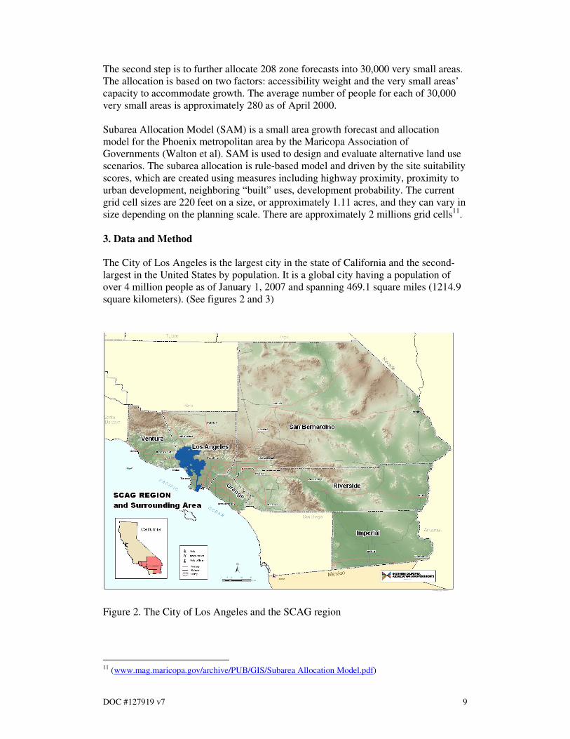
3. Data and Method

The City of Los Angeles is the largest city in the state of California and the second-

largest in the United States by population. It is a global city having a population of

over 4 million people as of January 1, 2007 and spanning 469.1 square miles (1214.9

square kilometers). (See figures 2 and 3)

Figure 2. The City of Los Angeles and the SCAG region

11 (www.mag.maricopa.gov/archive/PUB/GIS/Subarea Allocation Model.pdf)

DOC #127919 v7 10

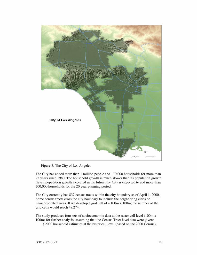
Figure 3. The City of Los Angeles

The City has added more than 1 million people and 170,000 households for more than

25 years since 1980. The household growth is much slower than its population growth.

Given population growth expected in the future, the City is expected to add more than

200,000 households for the 20 year planning period.

The City currently has 837 census tracts within the city boundary as of April 1, 2000.

Some census tracts cross the city boundary to include the neighboring cities or

unincorporated areas. If we develop a grid cell of a 100m x 100m, the number of the

grid cells would reach 48,274.

The study produces four sets of socioeconomic data at the raster cell level (100m x

100m) for further analysis, assuming that the Census Tract level data were given:

1) 2000 household estimates at the raster cell level (based on the 2000 Census);

DOC #127919 v7 11

2) 2005 household estimates at the raster cell level (based on the Claritas

household estimates as of January 1, 2006);

3) 2005 household estimates at the raster cell level (based on 2001 Regional

Transportation Plan (RTP) Household Forecasts at the Census Tract level, 1997-

2025);

4) 2025 household forecast at the raster cell level (based on 2001 RTP Household

Forecasts at the Census Tract level, 1997-2025).

3-1. Data

The study is based on a variety of data sources. The following is a brief overview of

the data sources.

Aerial Photography

SCAG has acquired a set of digital ortho-rectified photography for the entire region

including Mexicali, Mexico. The information was done at a 1-meter resolution for the

urban portions of the region which is equal to 9,133 square miles. The additional

29,000 square miles were done at 2 meter resolution.

Existing Land Use

In 2000, the Southern California Association of Governments (SCAG) developed a

digital land use coverage of its urban areas. The database covers the entire SCAG

region, approximately 38,500 square miles, including Mexicali, Mexico.

General Plan

City general plans are collected by SCAG from each local jurisdiction and are stored

in computerized format in SCAG's Geographic Information System (GIS). General

plans are constantly being updated by the individual cities. The land use in the general

plan is classified according to the Anderson (1971) land cover classification system.

To make the modeling process more manageable, SCAG collapsed the 100-plus land

use categories into seven: (i) undeveloped; (ii) single-family residential; (iii) multi-

family residential; (iv) commercial; (v) industrial; (vi) transportation; and (vii) public.

Census Tract Level Household Forecasts (7/1/2000, 7/1/ 2005, and 7/1/2025)

SCAG updates the growth forecast every three or four years. SCAG Regional Council

adopted a regional forecast, starting from 1997 to 2025, as part of the 2001 Regional

Transportation Plan (RTP), in April 2001. The 2001 RTP growth forecast was

developed in five year intervals between 2000 and 2025.

Claritas Tract Level Household Estimates (1/1/2006)

Claritas, a private vendor, has produced the updated demographic data every year for

more than 30 years. Tract Level Estimates are developed for January 1, 2006 by

incorporating many data sources. The data sources contributing to the 2006 tract level

estimates are: estimates produced by local governments or planning agencies, counts

of deliverable addresses from the U.S. Postal Service, household counts from the

Equifax Total Source consumer database, as well as counts from the Claritas Master

Address List.

Census Tract Level Household Estimates (4/1/2000)

DOC #127919 v7 12

The U.S. Census Bureau produces population and housing unit totals for Census 2000

at the census tract level. A census tract is a small, relatively permanent statistical

subdivision of a county or statistically equivalent entity, delineated for data

presentation purposes. Census tracts generally contain between 1,000 and 8,000

people12

.

Residential Building Permits for the City of Los Angeles (1/1/2001-12/31/2005)

The City of Los Angeles Planning Department keeps the recent residential building

permits issued between January 1, 2000 and December 31, 2005 for single- and

multiple-family housing units. This data is organized in the format of X/Y coordinates

and linked to the 2000 census tract.

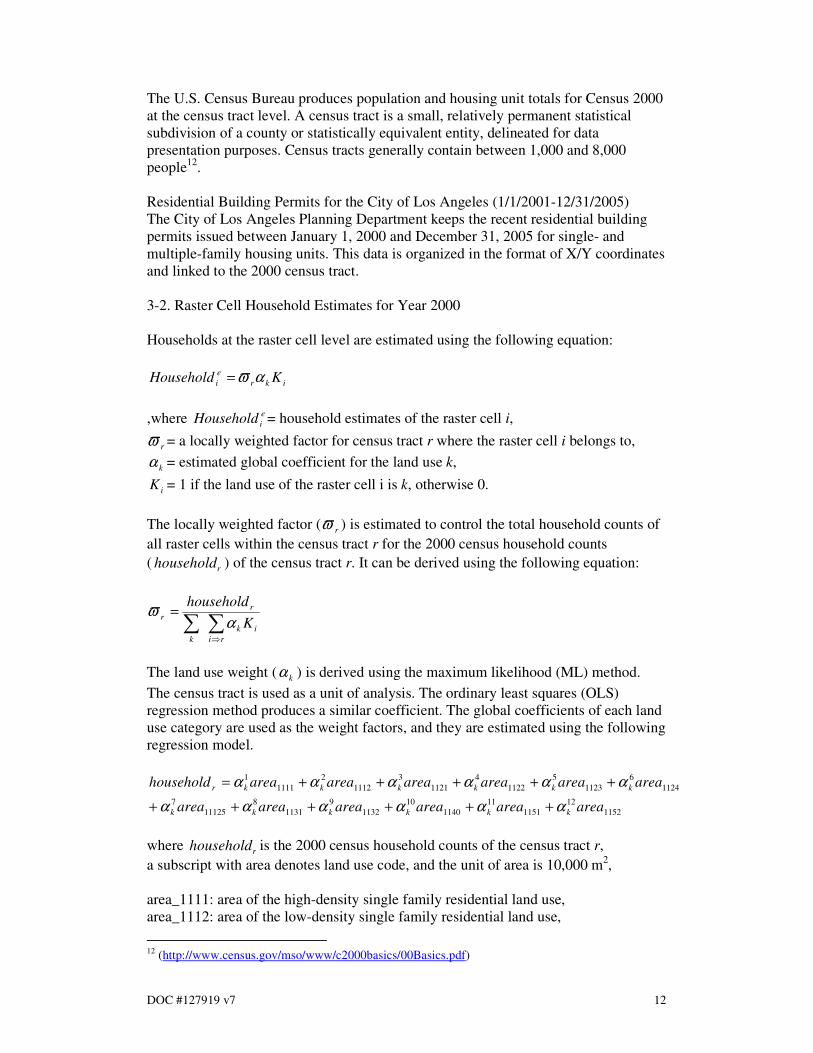
3-2. Raster Cell Household Estimates for Year 2000

Households at the raster cell level are estimated using the following equation:

ikr

e

i KHousehold αϖ=

,where e

iHousehold = household estimates of the raster cell i,

rϖ = a locally weighted factor for census tract r where the raster cell i belongs to,

kα = estimated global coefficient for the land use k,

iK = 1 if the land use of the raster cell i is k, otherwise 0.

The locally weighted factor ( rϖ ) is estimated to control the total household counts of

all raster cells within the census tract r for the 2000 census household counts

( rhousehold ) of the census tract r. It can be derived using the following equation:

∑∑⇒

=

ri

ik

k

r

rK

household

α

ϖ

The land use weight ( kα ) is derived using the maximum likelihood (ML) method.

The census tract is used as a unit of analysis. The ordinary least squares (OLS)

regression method produces a similar coefficient. The global coefficients of each land

use category are used as the weight factors, and they are estimated using the following

regression model.

1152

12

1151

11

1140

10

1132

9

1131

8

11125

7

1124

6

1123

5

1122

4

1121

3

1112

2

1111

1

areaareaareaareaareaarea

areaareaareaareaareaareahousehold

kkkkkk

kkkkkkr

αααααα

αααααα

++++++

+++++=

where rhousehold is the 2000 census household counts of the census tract r,

a subscript with area denotes land use code, and the unit of area is 10,000 m2,

area_1111: area of the high-density single family residential land use,

area_1112: area of the low-density single family residential land use,

12 (http://www.census.gov/mso/www/c2000basics/00Basics.pdf)

DOC #127919 v7 13

area_1121: area of the mixed multi-family residential land use,

area_1122: area of the duplexes, triplexes, and 2 or 3 unit condominiums and

townhouses land use,

area_1123: area of the low-rise apartments, condominiums, and townhouses land use,

area_1124: area of the medium-rise apartments and condominiums land use,

area_1125: area of the high-rise apartments and condominiums land use,

area_1131: area of the trailer parks and mobile home courts, high density land use,

area_1132: area of the mobile home courts and subdivisions, low density land use,

area_1140: area of the mixed residential land use,

area_1151: area of the rural residential, high-density land use,

area_1152: area of the rural residential, low-density land use.

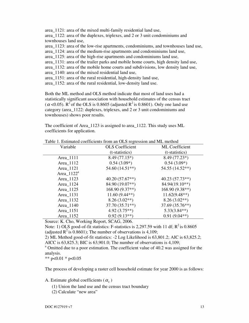
Both the ML method and OLS method indicate that most of land uses had a

statistically significant association with household estimates of the census tract

(α <0.05). R2

of the OLS is 0.8605 (adjusted R2

is 0.8601). Only one land use

category (area_1122: duplexes, triplexes, and 2 or 3 unit condominiums and

townhouses) shows poor results.

The coefficient of Area_1123 is assigned to area_1122. This study uses ML

coefficients for application.

Table 1. Estimated coefficients from an OLS regression and ML method

Variable OLS Coefficient

(t-statistics)

ML Coefficient

(t-statistics)

Area_1111 8.49 (77.15*) 8.49 (77.23*)

Area_1112 0.54 (3.09*) 0.54 (3.09*)

Area_1121 54.60 (14.51**) 54.55 (14.52**)

Area_1122a

Area_1123 40.20 (57.67**) 40.23 (57.73**)

Area_1124 84.90 (19.07**) 84.94(19.10**)

Area_1125 168.90 (9.37**) 168.90 (9.38**)

Area_1131 11.60 (9.44**) 11.62(9.48**)

Area_1132 8.26 (3.02**) 8.26 (3.02**)

Area_1140 37.70 (35.71**) 37.69 (35.76**)

Area_1151 4.92 (3.75**) 5.33(3.84**)

Area_1152 0.92 (9.13**) 0.91 (9.04**)

Source: K. Cho, Working Report, SCAG, 2006.

Note: 1) OLS good-of-fit statistics: F-statistics is 2,297.59 with 11 df; R2

is 0.8605

(adjusted R2

is 0.8601); The number of observations is 4,109;

2) ML Method good-of-fit statistics: -2 Log Likelihood is 63,801.2; AIC is 63,825.2;

AICC is 63,825.3; BIC is 63,901.0; The number of observations is 4,109; a Omitted due to a poor estimation. The coefficient value of 40.2 was assigned for the

analysis.

** p<0.01 * p<0.05

The process of developing a raster cell household estimate for year 2000 is as follows:

A. Estimate global coefficients ( kα )

(1) Union the land use and the census tract boundary

(2) Calculate “new area”

DOC #127919 v7 14

(3) Summarize the new area by the census tract and by the land use category

(4) Merge the result of A.(3) with the 2000 census household estimates

(5) Convert the land use categories to households using the estimated global

coefficients of the ML method.

B. Normalize the global coefficients to control for 2000 census tract estimates (krαϖ )

(1) Create a raster map (100m*100m grid) for each land use category by assigning

value 1 and repeat calculation for every land use category.

(2) Multiply the coefficient of A.(5) by the equivalent land category in the raster

map above and repeat calculation for every land use category.

(3) Mosaic all household related maps of B.(2)

(4) Produce “zonal statistics” by census tract.

(5) Create raster maps by using the sum of B.(4)

(6) Create probability maps by using the map algebra (B.(2)/ B.(5)). Use the

“raster calculator”.

C. Generate Raster Maps (ikr Kαϖ )

1) Create a raster map (100m*100m grid) with the census tract household data.

2) Multiply B.(3) by B.(6) using the “raster calculator.”

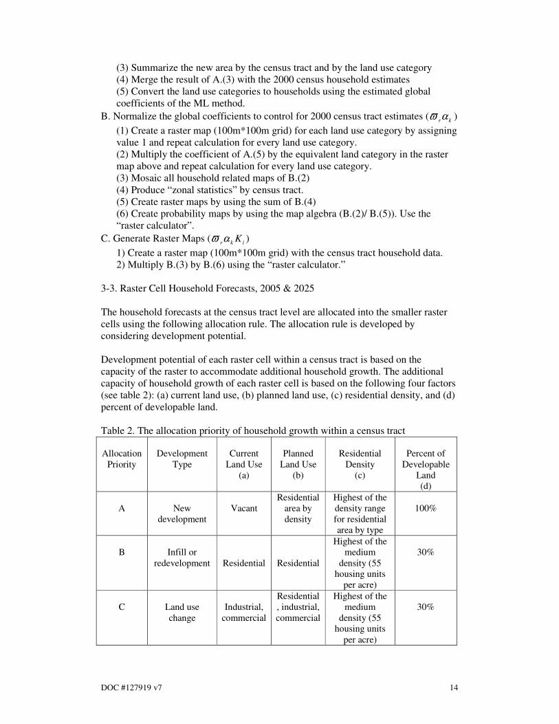
3-3. Raster Cell Household Forecasts, 2005 & 2025

The household forecasts at the census tract level are allocated into the smaller raster

cells using the following allocation rule. The allocation rule is developed by

considering development potential.

Development potential of each raster cell within a census tract is based on the

capacity of the raster to accommodate additional household growth. The additional

capacity of household growth of each raster cell is based on the following four factors

(see table 2): (a) current land use, (b) planned land use, (c) residential density, and (d)

percent of developable land.

Table 2. The allocation priority of household growth within a census tract

Allocation

Priority

Development

Type

Current

Land Use

(a)

Planned

Land Use

(b)

Residential

Density

(c)

Percent of

Developable

Land

(d)

A

New

development

Vacant

Residential

area by

density

Highest of the

density range

for residential

area by type

100%

B

Infill or

redevelopment

Residential

Residential

Highest of the

medium

density (55

housing units

per acre)

30%

C

Land use

change

Industrial,

commercial

Residential

, industrial,

commercial

Highest of the

medium

density (55

housing units

per acre)

30%

DOC #127919 v7 15

Note: Open space and other environmentally sensitive land are excluded from

additional household growth.

This study categorizes the current seven land use categories (e.g., undeveloped,

single-family residential, multi-family residential, commercial, industrial,

transportation, and public) into four: vacant; residential; commercial/industrial; and

other land use unsuitable for development.

The future land use plan specifies both land available and land not available for urban

development and redevelopment during the planning period (Berke et al, 2006). After

removing areas unsuitable for residential development, each raster cell is decomposed

into three major land development categories: 1) residentially developable vacant land,

2) residential infill/redevelopment, 3) industrial or commercial land. The process of

allocating census tract households into raster cell is as follows (see table 2):

A. Computing the maximum household growth capacity of residentially

developable vacant land: The maximum household growth capacity of

residentially developable vacant land is computed by multiplying each

residentially developable vacant land by maximum household density allowed in

the general plan of the City of Los Angeles.

B. Computing the additional household growth capacity of infill/redevelopment

land: The additional household growth capacity of infill/redevelopment land is

computed by multiplying 30% of existing residential areas by maximum

household density of the medium density residential areas allowed in the general

plan of the City of Los Angeles.

C. Computing the additional household growth capacity of industry and office

land uses: The additional household growth capacity of industry and office land

uses is computed by multiplying 30% of existing industry and office area by

maximum household density of the medium density residential areas allowed in

the general plan of the City of Los Angeles.

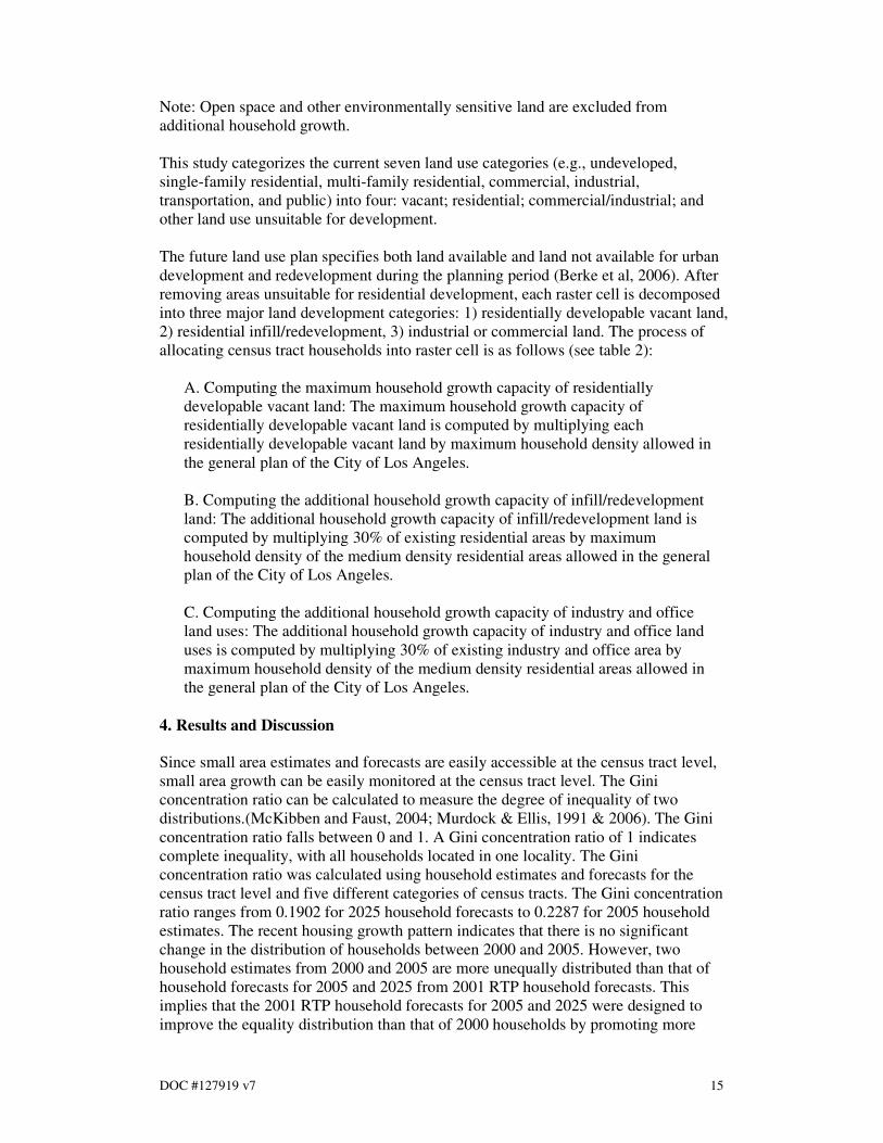
4. Results and Discussion

Since small area estimates and forecasts are easily accessible at the census tract level,

small area growth can be easily monitored at the census tract level. The Gini

concentration ratio can be calculated to measure the degree of inequality of two

distributions.(McKibben and Faust, 2004; Murdock & Ellis, 1991 & 2006). The Gini

concentration ratio falls between 0 and 1. A Gini concentration ratio of 1 indicates

complete inequality, with all households located in one locality. The Gini

concentration ratio was calculated using household estimates and forecasts for the

census tract level and five different categories of census tracts. The Gini concentration

ratio ranges from 0.1902 for 2025 household forecasts to 0.2287 for 2005 household

estimates. The recent housing growth pattern indicates that there is no significant

change in the distribution of households between 2000 and 2005. However, two

household estimates from 2000 and 2005 are more unequally distributed than that of

household forecasts for 2005 and 2025 from 2001 RTP household forecasts. This

implies that the 2001 RTP household forecasts for 2005 and 2025 were designed to

improve the equality distribution than that of 2000 households by promoting more

DOC #127919 v7 16

growth of the census tracts with less than 1,000 households, but in reality the more

equal distribution of households at the census tract level did not happen between 2000

and 2005.

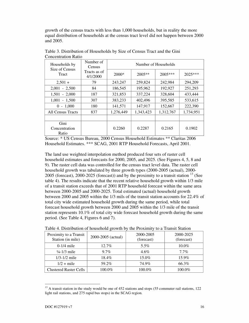
Table 3. Distribution of Households by Size of Census Tract and the Gini

Concentration Ratio

Number of Households Households by

Size of Census

Tract

Number of

Census

Tracts as of

4/1/2000 2000* 2005** 2005*** 2025***

2,501 + 79 243,247 259,824 242,984 294,209

2,001 - 2,500 84 186,545 195,962 192,927 251,293

1,501 - 2,000 187 321,853 337,224 328,604 433,444

1,001 - 1,500 307 383,233 402,496 395,585 533,615

0 - 1,000 180 141,571 147,917 152,667 222,390

All Census Tracts 837 1,276,449 1,343,423 1,312,767 1,734,951

Gini

Concentration

Ratio

0.2260 0.2287 0.2165 0.1902

Source: * US Census Bureau, 2000 Census Household Estimates ** Claritas 2006

Household Estimates. *** SCAG, 2001 RTP Household Forecasts, April 2001.

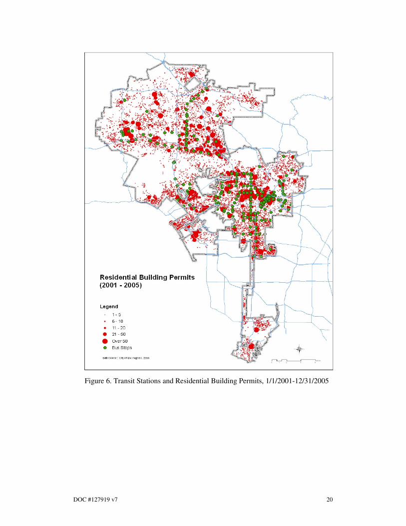
The land use weighted interpolation method produced four sets of raster cell

household estimates and forecasts for 2000, 2005, and 2025. (See Figures 4, 5, 8 and

9). The raster cell data was controlled for the census tract level data. The raster cell

household growth was tabulated by three growth types (2000-2005 (actual), 2000-

2005 (forecast), 2000-2025 (forecast)) and by the proximity to a transit station 13

(See

table 4). The results indicate that the recent relative household growth within 1/3 mile

of a transit station exceeds that of 2001 RTP household forecast within the same area

between 2000-2005 and 2000-2025. Total estimated (actual) household growth

between 2000 and 2005 within the 1/3 mils of the transit station accounts for 22.4% of

total city wide estimated household growth during the same period, while total

forecast household growth between 2000 and 2005 within the 1/3 mile of the transit

station represents 10.1% of total city wide forecast household growth during the same

period. (See Table 4, Figures 6 and 7).

Table 4. Distribution of household growth by the Proximity to a Transit Station

Proximity to a Transit

Station (in mile) 2000-2005 (actual)

2000-2005

(forecast)

2000-2025

(forecast)

0-1/4 mile 12.7% 5.5% 10.0%

¼-1/3 mile 9.7% 4.6% 7.7%

1/3-1/2 mile 18.4% 15.0% 15.9%

1/2 + mile 59.2% 74.9% 66.3%

Clustered Raster Cells 100.0% 100.0% 100.0%

13

A transit station in the study would be one of 452 stations and stops (55 commuter rail stations, 122

light rail stations, and 275 rapid bus stops) in the SCAG region.

DOC #127919 v7 17

The recent pattern of relatively fast household growth within walking distance from

the transit stations has two implications. The first implication is that the small area

growth can be used to update the household forecasts in the coming years. More

growth could be allocated into areas experiencing fast growth. The second implication

is that the small area growth within walking distance of stations is attributed to

strategic local and regional policies. The City’s multi-pronged efforts and SCAG’s

Compass Blueprint Program focus growth in existing and emerging centers and along

major transportation corridors. The City has implemented a transit vision strategy

which has been followed by major policy shifts and infrastructure investments. At a

regional level, SCAG adopted and is currently implementing the Compass Blueprint

Program whose proactive approach to planning and managing growth will create the

types of communities where all of us want to live work and play by providing tools

and services (such as fly through simulations and economic development strategies) to

cities and counties throughout Southern California to realize this growth vision on-

the-ground. The use of small area growth monitoring and the raster cell method in this

paper provides the opportunity to tell a story behind the possible scenarios to policy-

makers of the impact that future investments and policies can impact the makeup and

character of the City and the region at large.

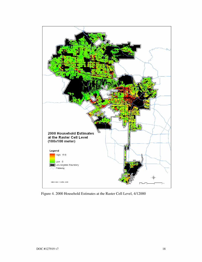
DOC #127919 v7 18

Figure 4. 2000 Household Estimates at the Raster Cell Level, 4/12000

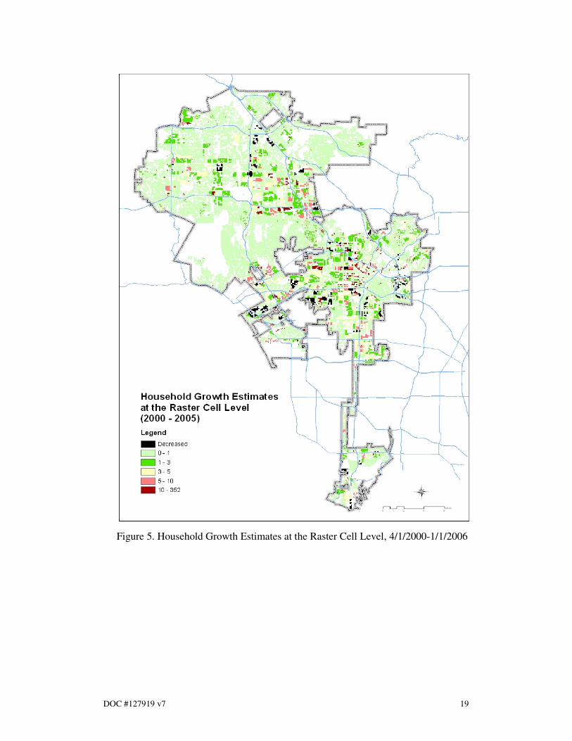
DOC #127919 v7 19

Figure 5. Household Growth Estimates at the Raster Cell Level, 4/1/2000-1/1/2006

DOC #127919 v7 20

Figure 6. Transit Stations and Residential Building Permits, 1/1/2001-12/31/2005

DOC #127919 v7 21

Figure 7. TOD Areas and Residential Building Permits 1/1/2001-12/31/2005

DOC #127919 v7 22

Figure 8. Household Growth Forecasts at the Raster Cell Level, 4/1/2000-7/1/2005

DOC #127919 v7 23

Figure 9. Household Growth Forecasts at the Raster Cell Level, 4/1/2000-7/1/2025

5. Conclusion

This paper presented a technique of monitoring small area growth with GIS.

Monitoring growth of small areas becomes an important tool in measuring the

progress of small area plans, such monitoring growth in and around transit oriented

development areas. This study used the land use weighted interpolation to develop

uneven and hopefully more accurate distribution of the socioeconomic estimates

within the census tract of the City of Los Angeles. The raster cell level socioeconomic

data estimates and forecasts were processed using land use information from both

DOC #127919 v7 24

aerial photographs and local general plans. The study also showed how

socioeconomic data at the raster cell level would be used to monitor the changing size

and spatial distribution of small area housing growth, in particular, around the transit

oriented development (TOD) area, to be able to provide additional information to

policy-makers about current and future changes that may result in the placement of

policies and investments.

Acknowledgment The authors thank Ying Zhou for providing the 2001 RTP household forecasts at the

census tract level and Jack Tsao for providing residential building permit data of the

City of Los Angeles.

DOC #127919 v7 25

References

Anderson, J. R., 1971, Land Use Classification Schemes Used in Selected Recent

Geographic Applications of Remote Sensing: Photogramm.Eng., v. 37, no. 4, p.

379—387.

Berke, R. P., D. R. Godschalk, and E. J. Kaiser with D. A. Rodriguez. 2006. Urban

Land Use Planning Fifth Edition. Illinois: University of Illinois Press.

Bollens, S. A. 1998. Land Supply Monitoring Systems. In the Growth Smart Working

Paper. Vol. 2. Chicago: American Planning Association.

Bourdier, J. 2006. Areal Interpolation Methods Using Land Cover and Street Data:

GIS Master’s Project.(http://charlotte.utdallas.edu/mgis/prj_mstrs/2006/Summer/Bourdier/report.pdf)

Brail, R. K. and R.E. Klosterman (eds.), 2001, Planning Support Systems. Redlands,

California: ESRI Press.

Cai, Q. 2004. A Methodology for Estimating Small-Area Population by Age and Sex

Based on Methods of Spatial Interpolation and Statistical Inference. GIScience 2004,

MD, USA

Childs, C., and G. Kabot. Working with ArcGIS Spatial Analyst.

Cho, K. 2006, Work Book, Southern California Association of Governments.

Claritas, 2006 Household Estimates at the census Tract Level.

Clark, M, and E. Holm. 1987. Microsimulation Methods in Human Geography and

Planning: A Review and Further Extensions, Geografisca Annalar 69B 145-164.

Eicher, C.L., and C.A. Brewer. 2001. Dasymetric Mapping and Areal Interpolation:

Implementation and Evaluation. Cartography and Geographic Information Science

28:125-138.

Enger, S. C. 1992. Issues in Designating Urban Growth Areas, Parts I and II.

Olympia, Washington: State of Washington, Department of Community Development,

Growth Management Division.

Fisher, P.F., and M. Langford,.1995. Modeling the Errors in Areal Interpolation

Between Zonal Systems by Monte Carlo Simulation. Environment and Planning A

27: 211-224.

George, M.V., S. K. Smith, D. A. Swanson, and J. Tayman. 2004. Population

Projections. Siegel, Jacob S. and David A. Swanson (eds.). The Methods and

Materials of Demography Second Edition. New York: Elsevier Academic Press.

Goodchild, M.F., and N. Lam. 1980. Areal Interpolation: A Variant of the Traditional

Spatial Problem. Geo- Processing 1: 297-312.

DOC #127919 v7 26

Goodchild, M. F., L. Anselin, and U. Deichmann. 1993. A Framework for the Areal

Interpolation of Socioeconomic Data. Environment and Planning A 25 (3): 383-

397.

Landis, J., and M. Zhang. 1998. The Second Generation of the California Urban

Futures Model: Parts I, II, and III. Environment and Planning B: Planning and Design.

25: 657-666, 795-824.

Landis, J. 2001. CUF, CUF II, and CUBRA: A Family of Spatially Explicit Urban

Growth and Land-Use Policy Simulation Models, In Brail, Richard K. and Richard E.

Klosterman (eds.), Planning Support Systems. Redlands, California: ESRI Press.

Langford, M. and Unwin, D. J. 1994. Generating and Mapping Population Density

Surfaces within a Geographical Information System. The Cartographic Journal, Vol

31, 21 – 26.

MacDougall, E.B., 1976. Computer Programming for Spatial Problems, Arnold,

London.

Martin, David. (1991) Geographic Information Systems and Their Socioeconomic

Applications, London: Routledge.

McCoy, J., and K. Johnston. 2001. Using ArcGIS Spatial Analyst. Redlands,

California: ESRI Press.

McKibben, J., and K. Faust. 2004. Population Distribution. In J. Siegel and D.

Swanson (Eds.) The Methods and Materials of Demography 2nd Edition. New York,

NY: Elsevier/Academic Press.

Mennis, J. and Hultgren, T., 2006. Intelligent dasymetric mapping and its application

to areal interpolation. Cartography and Geographic Information Science, 33(3): 179-

194.

Mennis, J., 2003. Generating Surface Models of Population Using Dasymetric

Mapping. The Professional Geographer, 55(1): 31-42.

Mennis, J., 2002. Using Geographic Information Systems to Create and Analyze

Statistical Surfaces of Population and Risk for Environmental Justice Analysis. Social

Science Quarterly, 83(1): 281-297.

Mouden, A. V., and M. H. Hubner. 2000. Monitoring Land Supply with Geographic

Information Systems: Theory, Practice, and Parcel-based Approaches. New York:

John Wiley & Sons.

Mugglin, A. S., B.P. Carlin, L. Zhu, and E. Conlon.1999. Bayesian Areal

Interpolation, Estimation, and Smoothing: An Inferential Approach for Geographic

Information Systems. Environment and Planning A, Vol 31, 1337 – 52.

Mugglin, A. S., B.P. Carlin, and A. E. Gelfand. 2000. Fully Model-Based Approaches

for Spatially Misaligned Data. Journal of the American Statistical Association, Vol 95,

DOC #127919 v7 27

No 451, 877 – 87.

Murdock, S.H., C. Kelley, and J. Jordan. 2006. Demographics: A Guide to Methods

and Data Sources for Media, Business, and Government. Boulder, Colorado:

Paradigm Publishers

Murdock, S.H., and D.R. Ellis. 1991. Applied Demography: An Introduction to Basic

Concepts, Methods, and Data. Boulder, Colorado: Westview Press.

Reibel, M., and A. Agrawal. 2006. Areal Interpolation of Population Counts Using

Pre-Classified Land Cover Data. Population Association of America Annual Meeting,

Los Angeles, March 31, 2006.

Sadahiro, Y. 1999. Statistical Methods for Analyzing the Distribution of Spatial

Objects in Relation to a Surface. Journal of Geographical Systems, 1 (2), 107-136.

Smith, S. K., J. Tayman, D. A. Swanson, 2001, State and Local Population

Projections: Methodology and Analysis, Kluwer Academic/Plenum Publishers, New

York.

Smith, S. K., and P. Morrison. 2005. Small-Area and Business Demography in

Dudley Poston and Michael Micklin, (eds). Handbook of Population. New York:

Kluwer Academic/Plenum Publishers.

Southern California Association of Governments. 2001 Regional Transportation Plan:

Household Forecasts.

Waddell P., and G. F. Ulfarsson. 2004. Introduction to Urban Simulation: Design and

Development of Operational Models. In Button, Kingsley, Hensher (eds). Handbook

in Transport, Volume 5: Transport Geography and Spatial Systems, Stopher:

Pergamon Press, pages 203-236.

Walton, R., M. Corlett, C. Arthur, and A. Bagley. Land Use and Transportation

Modeling with the ArcView Spatial Analyst: The MAC Subarea Allocation Model,

Maricopa Association of Governments.