mott-hubbard metal-insulator transition and optical conductivity in
TRANSCRIPT
Mott-Hubbard
Metal-Insulator Transition
and Optical Conductivity
in High Dimensions
Von der Mathematisch-Naturwissenschaftlichen Fakultatder Universitat Augsburg
zur Erlangung eines Doktorgrades der Naturwissenschaftengenehmigte Dissertation
vonDiplom–Physiker Nils Blumer
ausMunchen

i
Contents
Introduction 1
1 Models and Methods 5
1.1 Hubbard Model . . . . . . . . . . . . . . . . . . . . . . . . . . . . . . 5
1.1.1 Solid State Theory for Crystals . . . . . . . . . . . . . . . . . 6
1.1.2 Electronic Lattice Models . . . . . . . . . . . . . . . . . . . . 7
1.1.3 Wannier Representation . . . . . . . . . . . . . . . . . . . . . 8
1.1.4 One-band Hubbard Model . . . . . . . . . . . . . . . . . . . . 9
1.2 Dynamical Mean-Field Theory . . . . . . . . . . . . . . . . . . . . . . 11
1.2.1 Limit Z →∞ for Spin Models . . . . . . . . . . . . . . . . . . 12
1.2.2 Limit Z →∞ for Fermions . . . . . . . . . . . . . . . . . . . 13
1.2.3 Simplifications for the Hubbard Model in Z →∞ . . . . . . . 15
1.3 Quantum Monte Carlo Algorithm . . . . . . . . . . . . . . . . . . . . 19
1.3.1 Wick’s Theorem for the Discretized Impurity Problem . . . . 19
1.3.2 Monte Carlo Importance Sampling . . . . . . . . . . . . . . . 21
1.4 Maximum Entropy Method . . . . . . . . . . . . . . . . . . . . . . . 23
2 Lattice and Density of States 27
2.1 Hypercubic Lattice and Extensions . . . . . . . . . . . . . . . . . . . 29
2.1.1 Definitions and Analytical Considerations . . . . . . . . . . . 29
2.1.2 Numerical Results . . . . . . . . . . . . . . . . . . . . . . . . 32
2.1.3 Magnetic Frustration and Asymmetry of the DOS . . . . . . . 38
2.2 Bethe Lattice, RPE, and Disorder . . . . . . . . . . . . . . . . . . . . 39
2.2.1 Bethe Tree, Cayley Tree, and Husimi Cactus . . . . . . . . . . 40
2.2.2 Renormalized Perturbation Expansion . . . . . . . . . . . . . 43
2.3 General Density of States in d =∞ . . . . . . . . . . . . . . . . . . . 47
2.4 Redefinition of the Bethe Lattice . . . . . . . . . . . . . . . . . . . . 53
2.4.1 Model in d =∞ . . . . . . . . . . . . . . . . . . . . . . . . . . 54
2.4.2 Truncating the Hopping Range . . . . . . . . . . . . . . . . . 57
2.4.3 Finite Dimensionality . . . . . . . . . . . . . . . . . . . . . . . 59
2.4.4 Application to Asymmetric Model DOS . . . . . . . . . . . . . 62
2.5 Conclusion . . . . . . . . . . . . . . . . . . . . . . . . . . . . . . . . . 64
ii CONTENTS
3 Mott Metal-Insulator Transition in the d→∞ Hubbard Model 673.1 Motivation . . . . . . . . . . . . . . . . . . . . . . . . . . . . . . . . . 68
3.1.1 Experiment . . . . . . . . . . . . . . . . . . . . . . . . . . . . 683.1.2 Theory . . . . . . . . . . . . . . . . . . . . . . . . . . . . . . . 71
3.2 Characterization of Phase Transitions within the DMFT . . . . . . . 733.2.1 Transitions of First or Higher Order . . . . . . . . . . . . . . . 733.2.2 Convergence of Fixed Point Methods . . . . . . . . . . . . . . 753.2.3 Observables . . . . . . . . . . . . . . . . . . . . . . . . . . . . 76
3.3 Phase Diagram: Development until 1999 . . . . . . . . . . . . . . . . 793.4 Discussion of QMC Algorithms . . . . . . . . . . . . . . . . . . . . . 82
3.4.1 Fourier Transformation and Smoothing . . . . . . . . . . . . . 843.4.2 Overrelaxation and Sweeping Strategies . . . . . . . . . . . . . 893.4.3 Estimation of Errors . . . . . . . . . . . . . . . . . . . . . . . 903.4.4 Parallelization . . . . . . . . . . . . . . . . . . . . . . . . . . . 92
3.5 Results: Coexistence Region . . . . . . . . . . . . . . . . . . . . . . . 933.5.1 Choice of Observables and Extrapolation . . . . . . . . . . . . 933.5.2 Properties of the Insulating Phase . . . . . . . . . . . . . . . . 963.5.3 Internal Energy . . . . . . . . . . . . . . . . . . . . . . . . . . 1003.5.4 Coexistence Phase Diagram . . . . . . . . . . . . . . . . . . . 1083.5.5 Double Occupancy . . . . . . . . . . . . . . . . . . . . . . . . 113
3.6 Results: Thermodynamic Phase Transition Line . . . . . . . . . . . . 1213.6.1 Differential Equation for dUc /dT and Linearization . . . . . . 1213.6.2 Low-temperature Asymptotics of Uc(T ) . . . . . . . . . . . . . 1253.6.3 Full Phase Diagram . . . . . . . . . . . . . . . . . . . . . . . . 1313.6.4 Implications of Partial Frustration . . . . . . . . . . . . . . . . 138
3.7 Landau Theory and Criticality . . . . . . . . . . . . . . . . . . . . . . 1423.7.1 Free Energy Functional for the Bethe Lattice . . . . . . . . . . 1433.7.2 Direct Evaluation of Free Energy Differences . . . . . . . . . . 1443.7.3 Critical Behavior Near the MIT . . . . . . . . . . . . . . . . . 146
3.8 Spectra . . . . . . . . . . . . . . . . . . . . . . . . . . . . . . . . . . 1553.8.1 Maximum Entropy Method for Spectral Functions . . . . . . . 1553.8.2 Algorithmic Choices and Numerical Tests . . . . . . . . . . . . 1603.8.3 Numerical Results for the Bethe DOS . . . . . . . . . . . . . . 166
3.9 Conclusion . . . . . . . . . . . . . . . . . . . . . . . . . . . . . . . . . 173
4 Optical Conductivity 1754.1 Definition and General Properties of the Optical Conductivity . . . . 176
4.1.1 Connection between Conductivity and Reflectivity . . . . . . . 1774.1.2 Optical f -sum Rules . . . . . . . . . . . . . . . . . . . . . . . 1794.1.3 Experiments . . . . . . . . . . . . . . . . . . . . . . . . . . . . 1814.1.4 Impact of Electronic Model Abstractions . . . . . . . . . . . . 183
4.2 Kubo Formalism . . . . . . . . . . . . . . . . . . . . . . . . . . . . . 1864.2.1 Kubo Formalism in the Continuum . . . . . . . . . . . . . . . 1864.2.2 Kubo Formalism on a Lattice . . . . . . . . . . . . . . . . . . 1884.2.3 General Confirmation of the f -sum Rule . . . . . . . . . . . . 190
CONTENTS iii
4.3 Optical Conductivity in the Limit d→∞ . . . . . . . . . . . . . . . 1924.3.1 Optical Conductivity for the Hypercubic Lattice . . . . . . . . 1944.3.2 f -sum Rule within the DMFT . . . . . . . . . . . . . . . . . . 1954.3.3 f -sum Rule and General Dispersion Formalism . . . . . . . . . 197
4.4 Optical Conductivity for the Bethe Lattice . . . . . . . . . . . . . . . 1984.4.1 Treelike Layout of the Bethe Lattice . . . . . . . . . . . . . . 2004.4.2 Single-Chain Stacked Bethe Lattice . . . . . . . . . . . . . . . 2044.4.3 Periodically Stacked Lattices . . . . . . . . . . . . . . . . . . . 2094.4.4 Offdiagonal Disorder . . . . . . . . . . . . . . . . . . . . . . . 2114.4.5 General Dispersion Method . . . . . . . . . . . . . . . . . . . 213
4.5 Generalizations . . . . . . . . . . . . . . . . . . . . . . . . . . . . . . 2164.5.1 Coherent versus Incoherent Transport in High Dimensions . . 2164.5.2 Optical Conductivity in Finite Dimensions . . . . . . . . . . . 2194.5.3 Impact of Frustration by t− t′ Hopping . . . . . . . . . . . . . 222
4.6 QMC Results for the Bethe Lattice . . . . . . . . . . . . . . . . . . . 2254.6.1 Numerical Procedure for QMC Data . . . . . . . . . . . . . . 2264.6.2 Results: Self-Energy on the Real Axis . . . . . . . . . . . . . . 2304.6.3 Results: Optical Conductivity . . . . . . . . . . . . . . . . . . 234
4.7 Conclusion . . . . . . . . . . . . . . . . . . . . . . . . . . . . . . . . . 242
5 Realistic Modeling of Strongly Correlated Materials 2455.1 La1-xSrxTiO3 . . . . . . . . . . . . . . . . . . . . . . . . . . . . . . . 2465.2 DFT and LSDA . . . . . . . . . . . . . . . . . . . . . . . . . . . . . . 2495.3 LDA+DMFT . . . . . . . . . . . . . . . . . . . . . . . . . . . . . . . 2515.4 Results for La1-xSrxTiO3 . . . . . . . . . . . . . . . . . . . . . . . . . 255
5.4.1 Density of States and Photoemission Spectra . . . . . . . . . . 2555.4.2 Influence of Discretization Errors . . . . . . . . . . . . . . . . 2615.4.3 Optical Conductivity . . . . . . . . . . . . . . . . . . . . . . . 268
5.5 Conclusion . . . . . . . . . . . . . . . . . . . . . . . . . . . . . . . . . 276
Summary 279
A Additions to “Models and Methods” 281A.1 Extensions of the Hubbard Model . . . . . . . . . . . . . . . . . . . . 281A.2 Characterization of Generic Momenta . . . . . . . . . . . . . . . . . . 284A.3 DCA, CDMFT, and RDA . . . . . . . . . . . . . . . . . . . . . . . . 286
B Hyperdiamond Lattice 291
C Fourier-Transforming Imaginary-Time Green Functions 297
D Linear Response to Electromagnetic Fields 305D.1 Electromagnetic Interaction Hamiltonian and Choice of Gauge . . . . 305D.2 Linear Response Theory . . . . . . . . . . . . . . . . . . . . . . . . . 306
Bibliography 309

iv CONTENTS
Index 321
List of Publications 331
Curriculum Vitae 333
Acknowledgements 335

v
Nomenclature
0+ Positive infinitesimal
〈〈B, A〉〉 Correlation function, p. 308
〈f(ε)〉 Thermal expectation value,p. 195
〈f(ε)〉ρ(ε) Expectation value, p. 31
〈f(k)〉k Expectation value, p. 31
〈〈i, j〉〉 NNN pairs (in summation),p. 31
〈i, j〉 NN pairs (in summations), p. 9
s Auxiliary Ising spin field, p. 20
|v| Euclidean metric, 2-norm, p. 29
||v|| “Taxi cab” vector metric,1-norm, p. 30
α, β, γ Cartesic indices
β Inverse temperature, p. 17
ε(ω) Dielectric function, p. 177
εk, ε(k) Electronic dispersion(noninteracting energy), p. 14 +47
εD(k) Contribution to dispersion fromhopping to Dth-NN, p. 47
ηq DMFT momentum transferparametrization, p. 14
Λ Number of time slices, p. 19
Λ NRG frequency discretization,p. 111
µ Chemical potential, p. 10
µ, ν Band indices, p. 8
ρ(ε) Noninteracting DOS, p. 28
ρ(ε) Lattice input for σ(ω), p. 28
ρ′(ε) Derivative of ρ(ε), p. 195
Σ Proper self-energy, p. 16
σ Electronic spin, p. 8
σ0 Prefactor for σ(ω), p. 193
σ(ω) Optical conductivity, p. 177 +189
τ , ∆τ Imaginary time (p. 17), Trotterdiscretization (p. 19)
τ Hopping vector, p. 47
τ l Primitive lattice vector, p. 291
ψ Field operator, p. 8
ψ,ψ∗ Grassmann variables, p. 17
ωn Matsubara frequency, p. 16
ωp Plasma frequency, p. 180
a Asymmetry of model DOS(p. 43), lattice spacing (p. 188)
a∗ Ratio of scaled hoppingamplitudes for hc lattice withNN and NNN hopping, p. 31
vi Nomenclature
an Weight of self-avoiding loops oflength n, p. 44
a1g Atomic orbitals, p. 281
A Single-site action, p. 17
A(ω) Full single-particle spectralfunction, p. 23
Aε(ω) “k-resolved” spectral function,p. 193
A Electromagnetic vectorpotential, p. 305
A, B Sublattices of a bipartitelattice, p. 32
c†iσ,ciσ Creation, annihilation operator,p. 9
c†iνσ,ciνσ Creation, annihilation operator(multi-band), p. 8
c Speed of light, p. 305
C General matrix or tensor(p. 293), covariance matrix(p. 157)
d Differential operator
dx Infinitesimal volume ddx
d Band character in atomic limit(s, p, d, f ,. . . ), p. 281
d Dimension, p. 10
Dq(ε1, ε2) Two-particle density of states,p. 14
D[ψ] Functional differential, p. 17
erf(x) Error function (of x)
e Euler’s number (ex ≡ exp(x))
eα Cartesic unit vector, p. 30
e Electronic chargee ≈ −1.6× 10⁻¹⁹C, p. 6
eg, eπg Atomic orbitals, p. 281
E Electric field, p. 176
F(x) DOS transformation function,p. 49
F0 Multi-band model parameter,p. 282
G, G0 Full vs. noninteracting Greenfunction, p. 16
Gε(iωn) “Momentum-dependent” Greenfunction, p. 78
G Effective local bath propagator,p. 17
Hen(x) Hermite polynomial, p. 49
H, H Hamiltonian
HHub Hubbard Hamiltonian, p. 9
Imx Imaginary part (of x)
j, Paramagnetic current density(operator), p. 186
J Total current, p. 176
k Lattice momentum, p. 8
K Connectivity for Bethepseudo-lattice, p. 40
K, K0 Kinetic energy with (without)coupling to A, p. 188
L Number of ions (p. 6), numberof lattice sites (p. 8)
m Electronic massm ≈ 9.1× 10⁻³¹kg, p. 6
m∗ Effective (electron) mass, p. 76
niσ Occupation of lattice site i forspin σ, p. 9
n Average band filling, p. 10
nε,σ, nε Momentum distributionfunction, p. 196
Nomenclature vii
nf(ω) Fermi function, p. 193
Ne, Nv Number of electrons (p. 6),number of valence electrons(p. 7)
O(xn) Of the order xn
P Polarization operator, p. 190
q Lattice momentum, momentumtransfer, p. 14
Q Antiferromagnetic wave vector,p. 14
Rex Real part (of x)
r Distance, radius, p. 6
R Position of ion or lattice site,p. 6
Siν , siν Spin operator, p. 282
t NN hopping matrix element,p. 9
tνij Hopping matrix elementbetween sites i and j in band ν,p. 8
tD Hopping matrix element for(taxi cab) distance D, p. 38 +48
t2g Atomic orbitals, p. 281
Tr
Trace
T Temperature, p. 10
U Hubbard on-site interaction,p. 9
v Generic vector
vk, vk,ν Fermi velocity, p. 185
V0 Multi-band model parameter,p. 282
x Generic variable
Z Lattice coordination number,p. 11
Z Quasiparticle weight, p. 76
Z Partition function, p. 17
AF Antiferromagnet(ic), p. 10
ASA Atomic sphere approximation,p. 251
CDMFT Cellular (or cluster) DMFT,p. 286
DCA Dynamical clusterapproximation, p. 286
DFT Density functional theory,p. 249
DMFT Dynamical mean-field theory,p. 11
DMRG Density matrix renormalizationgroup, p. 289
DOS Noninteracting density ofstates, p. 14
ED Exact Diagonalization, p. 18
EELS Electronic energy lossspectroscopy, p. 183
FLEX Fluctuation-exchangeapproximation, p. 18
HF Hartree-Fock theory, p. 11
IPT Iterated perturbation theory,p. 18
L(S)DA Local (spin) densityapproximation, p. 250
LMTO Linear muffin-tin orbitals,p. 251
MEM Maximum entropy method,p. 25
NCA Non-crossing approximation,p. 18

viii Nomenclature
NN Nearest neighbors, p. 9
NNN Next-nearest neighbors, p. 27
NRG Numerical renormalizationgroup, p. 18
PES Photoemission spectroscopy,p. 258
QMC Quantum Monte Carlo, p. 19
RDA Random dispersionapproximation, p. 288
SIAM Single impurity Andersonmodel, p. 11
XAS X-ray absorption spectroscopy,p. 268
f -sum Sum rule for σ(ω), p. 179
fcc (Hyper) face centered cubic(lattice), p. 32
hc Hypercubic (lattice), p. 27
hd Hyperdiamond (lattice), p. 291
1
Introduction
Solid state theory aims at a description of intrinsic properties of solid materials byfinding and extracting information from suitable models. A good model is com-plicated enough to capture interesting aspects of nature, but simple enough to besolvable (at least within some limits or within controlled approximations) and to pro-vide insights about the associated mechanisms. Even if it was possible to constructa theory which exactly predicts all measurable properties of solids, more abstractmodels would still be necessary in order to classify the different properties and thedifferent classes of physical systems and in order to identify which “ingredients” areimportant for some particular effect. In this sense, the presence of free parametersin model Hamiltonian approaches is not necessarily a shortcoming compared to abinitio methods, but a very useful handle for understanding phenomena in a generalcontext. Often, different simplified models give reasonable descriptions for differentproperties of the same material. For a more realistic description one can then buildup a hierarchy of more complex theories, thus broadening the range of validity andimproving on the accuracy of agreement to experiment. The main advantage of a mi-croscopic model over a phenomenological theory is that its inherent approximationsare known so that it can, at least in principle, be made more realistic in a controlledway.
Solids are constituted of a macroscopic number of positively charged atomic nucleiand negatively charged electrons. In single crystals, the heavy nuclei can be assumedto form a rigid periodic lattice. Furthermore, due to the strong Coulomb force, alarge fraction of the electrons is typically tightly bound in atomic-like shells aroundthe ions. The resulting core ions then provide a periodic background potential forand shield the interaction between the remaining electrons. These valence electronsdetermine, to leading order, the electronic, magnetic, and thermal properties of solids.In this work, we will exclusively study the electronic system and mostly restrict ourtreatment to the valence electrons.
Even in the limit of vanishing interaction between the (valence) electrons, theirdispersion is split by the lattice potential into an infinite number of energy bands(Bloch, 1928). Due to the Pauli exclusion principle each eigenstate, characterizedby its momentum (within the Brillouin zone), band index, and spin, can only beoccupied by one electron. Consequently, there is some trivial correlation betweenthe electrons even at the noninteracting level. The (lattice-dependent) energy ofnoninteracting electrons is commonly referred to as kinetic energy. It is the potentialenergy associated with the (shielded) electron-electron Coulomb interaction whichintroduces genuine correlations between the valence electrons and makes the problem

2 Introduction
interesting and complicated.
The low-energy electronic properties of some materials can be reasonably wellunderstood without explicitly taking electron-electron interactions into account. Forgood metals, this surprising fact is elucidated by the phenomenological Landau Fermi-liquid theory (Landau, 1957a; Landau, 1957b) which replaces electrons by noninter-acting quasiparticles with a renormalized mass and a finite lifetime. Even whenthe noninteracting picture fails, phenomena such as long-range order can some-times be described within a static mean-field theory; here one replaces the effectof the electron-electron interaction on each electron by that of a time averaged (andpossibly spin-dependent) electronic charge density. In general however, in partic-ular for transition metal compounds, such effective single-particle pictures fail tosatisfactorily reproduce the interesting physical phenomena. These strongly cor-related electron systems, for which the transition metal compounds are prototypeexamples due to the strong (and locally essentially unshielded) Coulomb interac-tion between their well-localized 3d and 4f valence orbitals, then call for theo-ries which retain the full dynamics of the electronic correlation problem. Theo-ries for such d and f systems typically take only few orbitals per lattice site intoaccount and assume an effectively short-ranged Coulomb interaction. An extremecase is the Hubbard model where the Coulomb interaction is reduced to its on-sitepart (Hubbard, 1963; Gutzwiller, 1963; Kanamori, 1963), i.e., where electrons onlyinteract with each other if they occupy the same lattice site (in the Wannier picture).
The Dynamical Mean-Field Theory (DMFT) is a nonperturbative approximationfor strongly correlated electron models, namely variants of the Hubbard model, whichbecomes exact in the limit of infinite dimensionality or, equivalently, infinite latticecoordination number (Metzner and Vollhardt, 1989). It neglects (short-range) spa-tial correlations between the electrons while it retains their dynamical correlationswhich are crucial for the description of many interesting phenomena observed incorrelated electron systems. The DMFT simplifies the lattice problem by mappingit onto a single-impurity model embedded in a medium that has to be determinedself-consistently. Still, explicit solutions can only be obtained by application of ei-ther further approximations or of numerical techniques. The quantum Monte Carlo(QMC) method is numerically exact, i.e., its error can in principle be made arbi-trarily small by increasing the numerical effort; even with today’s high-performancecomputers the method is, however, restricted to not too low temperatures.
The low-temperature electronic properties of materials can be classified as insu-lating, metallic, or superconducting depending on whether the resistivity increasesor decreases upon lowering the temperature or precisely vanishes (below some crit-ical temperature), respectively. Changes in the resistivity and, in particular, phasetransitions from a metallic to an insulating state can be induced by, e.g., changeof stoichiometric composition, pressure, temperature, or magnetic field or by intro-ducing disorder. In contrast to transitions to (possibly long-range ordered) bandinsulators or those induced by Anderson localization which can be understood ona noninteracting or static mean-field level, nonperturbative approaches are requiredfor a quantitative theory of the correlation-induced Mott metal-insulator transition(MIT) which occurs at a point where potential and kinetic energy are of the same
Introduction 3
order.
The main focus of this work are studies of correlated electron systems near a Mottmetal-insulator transition. In particular, we will present the first controlled DMFTcalculation of the complete phase diagram of the fully frustrated single-band Hubbardmodel with semi-elliptic density of states at half filling using the QMC method. Wewill also perform the first calculations of the associated optical conductivity whichdo not depend on the assumption of anisotropy or disorder; these will be based onthe general theory of densities of states and transport properties in high dimensionswhich is also developed in this thesis. In addition to these pure model studies, wewill present results specific to the doped transition metal oxide La1-xSrxTiO3 whichare obtained using the hybrid LDA+DMFT technique. This new method employsab initio density functional theory in the local density approximation (LDA) fordefining a general multi-band Anderson-Hubbard model which is then treated withinthe DMFT.
Structure of this Thesis
In chapter 1, we introduce the general electronic Hamiltonian and its reduction tothe Hubbard model. We characterize the DMFT and its relation with mean-field ap-proximations to spin systems and present the DMFT mean-field equations as well astheir solution using the auxiliary-field QMC method. Finally, we discuss the analyticcontinuation of imaginary-time Green functions to the real axis by the maximumentropy method (MEM).
In chapter 2, we study the relations between lattice types, frustration, and densi-ties of states (DOS). On the basis of Monte Carlo computations of momentum sums,we also evaluate the convergence of the density of states to its infinite-dimensionallimit. We present new insights on the fractal tree commonly referred to as Bethelattice and on the impact of longer-range hopping for this model. We develop a newformalism that allows to construct models with hypercubic symmetry which repro-duce an arbitrary target DOS in the limit of infinite dimensionality (d =∞). Usingthis approach, we can for the first time define a regular and translationally invariantlattice with semi-elliptic DOS in d =∞.
In the central chapter 3, we thoroughly explore the low-temperature propertiesof the fully frustrated Hubbard model with semi-elliptic DOS within the DMFT. Wedetermine the boundaries of a coexistence region of metallic and insulating solutionswith high accuracy, thereby resolving a controversy on the existence of a first-ordertransition within this model. In the course of these studies, we detect and correctdeficiencies in previously used QMC schemes and develop an improved criterion forthe detection of phase transitions. Going beyond previous work, we also developa method for a reliable determination of the first-order transition line and performvarious tests of the accuracy of the result. Finally, we compute local MEM spectraand suggest some methodological improvements to be used in future calculations.
Transport properties are discussed in chapter 4, where we carefully review theformalism and its range of applicability and develop new expressions for the opticalf -sum rule which are valid in d = ∞. We show that the correct consideration of
4 Introduction
lattice properties is quantitatively important also in this limit and that simplifyingassumptions made in a previous study on the impact of frustration lead to large errors.We point out the ambiguities associated with any DMFT calculation of transportproperties for “the Bethe lattice” and review the possible concepts for making theproblem well-defined; among these choices, the model defined in chapter 2 will be seento have the most desirable properties. We then present accurate numerical results forthe optical conductivity which are based on the MEM spectra computed in chapter 3.
In chapter 5, we give an introduction to the density functional theory and its lo-cal density approximation and introduce the recently developed hybrid LDA+DMFTscheme. We discuss the construction and simplification of the resulting multi-bandHubbard model and its solution within the DMFT as well as the extraction of pho-toemission and x-ray absorption spectra. In addition to numerical results obtainedin a collaboration with Anisimov’s group, we present new calculations and quantifythe QMC discretization error. We also apply the formalism developed in chapter 2in order to derive a definition of the optical conductivity which is compatible withthe LDA DOS and present corresponding numerical results.
With the exception of the following introductory part, each chapter is supple-mented by a conclusion. A brief overview over the results and new insights obtainedin this thesis is given in the Summary. Finally, some aspects not directly within themain scope of this thesis are treated in the appendices.
5
Chapter 1
Models and Methods
In this chapter we set the framework for the main part of this thesis by introducing themodels under investigation and the approximations and methods employed. Studiesof abstract models represent an idealized and focused view on physics which shouldbe complemented by a clear knowledge about the inherent limitations. Therefore,we will emphasize those steps of abstraction from a “complete model” to the modelsstudied in this work which potentially cause properties of the resulting theory todiffer qualitatively from seemingly corresponding properties of real materials. Later,we will make contact with these observations, e.g., in the discussion of the f -sum ruleof the optical conductivity (see chapter 4) and discuss a more complete picture in thecontext of the LDA+DMFT method and its application to La1-xSrxTiO3 in chapter 5.Since the density functional theory (DFT) and its local density approximation (LDA)are not central to this work, these approaches are introduced directly in the context oftheir application in chapter 5. As far as practical, methods like the quantum MonteCarlo (QMC) algorithm or the maximum entropy method (MEM) are covered here ona descriptive level while original methodological contributions are mainly discussedin the following chapters.
In the following, we will first discuss the Hubbard model in a general context inSec. 1.1, then its nonperturbative treatment within the dynamical mean-field theory(DMFT) in Sec. 1.2. We describe the quantum Monte Carlo method of solving theDMFT self-consistency equations in Sec. 1.3 and the maximum entropy method of ob-taining real-time dynamical information by analytic continuation of QMC imaginary-time data in Sec. 1.4.
1.1 Hubbard Model
The one-band Hubbard model is the minimal lattice model for strongly correlatedelectron systems, i.e., for describing electronic properties of materials which cannotbe treated without explicitly taking the Coulomb interaction between the (valence)electrons into account. Typical examples are the transition metals and their com-pounds. In subsections 1.1.1 – 1.1.4, we explore the microscopic foundation of theHubbard model and review some of its basic properties and limitations. Extensionsof the one-band Hubbard model which can potentially overcome some of these limi-
6 1. Models and Methods
tations are listed in App. A.1. While most of these extensions are beyond the scopeof this thesis, the multi-band model (A.5) will be central to chapter 5.
1.1.1 Solid State Theory for Crystals
The typical condensed matter system contains a macroscopic number (usually 1020
or more) of atomic nuclei and electrons.1 In this situation, a complete description ofa particular system for given initial conditions is not possible. In fact, it might notbe desirable since the truly interesting information would be hidden in an extensiveamount of details. It is the concept of statistical physics to abstract from some specificsystem and view it as a realization of an ensemble of systems which share only someimportant features like the atomic constitution exactly but are allowed to differ inothers. Among the observations that can be made for such ensembles are not onlythose that pertain to each individual realization (like energy conservation), but alsoothers that involve averages over the ensemble, over time, and/or over space (likedensity-density pair correlation functions).2 All results of this work will apply to thethermodynamic limit of a (grand) canonical ensemble of unbounded systems with nonet charge.
Neglecting intra-nuclear effects and the gravitational, “weak”, and “strong” forces(which are extremely small on typical condensed matter length scales of 10−10 m to 1m), we assume that condensed matter systems are composed of inert pointlike atomicnuclei and electrons which interact by the Coulomb 1/r potential (for a distance r)and have no internal degrees of freedom other than (possibly) spin. Although, ingeneral, relativistic effects are important for the systems under consideration, theyoften contribute only a constant energy offset to the solid-state problem (e.g., for corestates of heavy nuclei) or can be treated approximately in a nonrelativistic framework(e.g., spin-orbit coupling for valence electrons; see App. A.1). Thus, the usual startingpoint for condensed matter theory is nonrelativistic quantum statistical mechanics forcharged electrons and ions with the Hamiltonian3
H =Ne∑
i=1
p2i
2m+
L∑
k=1
P 2k
2Mk
+∑
i<j
e2
|ri − rj|+∑
k<l
ZkZle2
|Rk −Rl|−∑
i,k
Zke2
|ri −Rk|(1.1)
Here, ri (Rk), pi (P i), and m (Mk) label the positions, momenta, and masses of elec-trons (ions), respectively; e is the electronic charge, Ne the total number of electrons,L that of ions, and Zk the atomic number of the ion with index k. Charge neutralityrequires that Ne =
∑
k Zk. In the Gaussian system of units, 4πε0 = 1 drops out ofthe expressions for the Coulomb energy.
1Exceptions to this rule are, e.g., mesoscopic systems where the physics may be dominated byfinite-size effects like in the single-electron transistor.
2Note that for ergodic systems, the infinite-length limit of the time average by definition agreeswith the ensemble average.
3The discussion of couplings to external electromagnetic fields is deferred to Sec. 4.2. We noteat this point, however, that the assumption of instantaneous Coulomb interaction used here and inthe following is exact within the Coulomb gauge.
1.1. Hubbard Model 7
Since the long-range mobility of ions is vanishingly small in the solid state (exceptfor solid Helium), one can estimate the kinetic energy of the ions to be smaller thanthat of the electrons by a factor of (m/Mk)
1/2 ≈ 10−2 − 10−3, which suggests usingm/M as a perturbation parameter where M is, e.g., the smallest ion mass in thesystem. In the adiabatic approximation (Born and Oppenheimer, 1927) one treats theelectronic problem for fixed ion coordinates; feeding back the electronic eigenenergiesas a function of the ion coordinates then allows for an approximate treatment of theionic contribution which reduces the error to (m/M)3/4 (see, e.g., Czycholl, 2000).We will take the zeroth-order approximation, i.e., use immobile ions on a periodiclattice and view them as an external potential for the electrons. The effect of thisconsiderable simplification should be kept in mind when later interpreting results, inparticular with respect to transport properties.
1.1.2 Electronic Lattice Models
The resulting purely electronic Hamiltonian,
H =Ne∑
i=1
p2i
2m+∑
i
V (ri) +∑
i<j
e2
|ri − rj|, (1.2)
where the external potential V (r) = V (r + Rα) is periodic on the lattice (withprimitive lattice vectors Rα for α = 1, . . . , d, where d is the dimension), defines theelectronic lattice problem.
A full solution of this problem would have to include energy contributions (ofpositive and negative sign) of at least the highest x-ray absorption edge of the con-stituting atoms, which can be more than 6 orders of magnitude larger than energydifferences between, e.g., metallic and insulating phases considered in this work. Inthis situation it is useful to distinguish between core electrons and valence electronswhere the former are assumed to be tightly bound to the nuclei. The resulting new“elementary particles”, the core ions, then define a new, drastically weaker crystalpotential. Since core ions are polarizable they also modify the infinite-range 1/rpotential of the bare Coulomb electron-electron interaction to some shorter rangedform.4 Provided that these effects can be quantified, we may restrict the treatmentto few valence electrons per lattice site,
H =Nv∑
i=1
p2i
2m+
Nv∑
i=1
V ion(ri) +Nv−1∑
i=1
Nv∑
j=i+1
V ee(ri, rj), (1.3)
where Nv is the number of valence electrons and V ion the shielded lattice potential.Here, we have implicitly assumed an instantaneous effective interaction of the density-density type which is certainly not exact. We also point out that the (screened)effective interaction potential V ee between valence electrons is in general neitherhomogeneous nor isotropic since the shielding charges are localized. Now switching
4Valence electrons can also take part in shielding the electron-electron interaction. This effectshould, however, not be built into a microscopic valence-electron model, but result from its solution.
8 1. Models and Methods
to the occupation number formalism (“second quantization”; see, e.g., Fetter andWalecka, 1971) in real space, the Hamiltonian for electrons with spin σ takes theform
H = H0 + Hint, (1.4)
where
H0 =∑
σ
∫
dr ψ†σ(r)
[
− ~2
2m∆ + V ion(r)
]
ψσ(r) (1.5)
Hint =1
2
∑
σσ
∫
dr
∫
dr ′ V ee(r, r′) nσ(r) nσ′(r′) . (1.6)
Here, ψσ(r), ψ†σ(r) are field operators which annihilate and create electrons of spin σ
at site r, respectively; ~ = h/2π is Planck’s constant, ∆ the Laplace operator, andnσ(r) = ψ†
σ(r)ψσ(r) the operator measuring the local density of electrons with spinσ at position r.
1.1.3 Wannier Representation
In terms of the lattice momentum k and Bloch eigenfunctions φνk(r) of the non-interacting5 Hamiltonian (1.5), we may introduce Wannier functions predominantlylocalized at site Ri by
χiν(r) =1√L
∑
k
e−ik·Ri φkν(r) , (1.7)
where L is the number of lattice sites, and thus construct creation and annihilationoperators c†iνσ,ciνσ for electrons with spin σ ∈ ↑, ↓ in the band ν at site Ri as
c†iνσ =
∫
dr χiν(r) ψ†σ(r) ←→ ψ†
σ(r) =∑
iν
χ∗iν(r)c†iνσ . (1.8)
Using this basis, the Hamiltonian may be written in the lattice representation as(Hubbard, 1963; Hubbard, 1964a)
H =∑
iνjσ
tνij c†iνσ cjνσ +
1
2
∑
νν′µµ′
∑
ijmn
∑
σσ′
Vνν′µµ′ijmn c†iνσ c†jν′σ′ cnµ′σ′ cmµσ , (1.9)
where the matrix elements are given by
tνij =
∫
dr χ∗iν(r)
[
− ~2
2m∆ + V ion(r)
]
χjν(r) (1.10)
Vνν′µµ′ijmn =
∫
dr
∫
dr ′ V ee(r, r ′)χ∗iν(r) χ∗
jν′(r′) χnµ′(r
′) χmµ(r) . (1.11)
5In principle, we mean by “noninteracting” the absence of interaction between electrons. Inpractice, however, it is often necessary to assume that at least a long-range Hartree part of theinteraction between the valence electrons is also included as a part of the kinetic energy and usedfor the definition of the Wannier orbitals (Gebhard, 1997) which then better justifies a very short-ranged form of the remaining explicit interaction. In any case, however, we want to assume that theexternal potential need not be determined self-consistently (which might affect conclusions aboutphenomena such as phase separation).
1.1. Hubbard Model 9
Several observations can be made at this point: First of all, in contrast to thefield-operator representation defined in the continuum, in the Wannier representationeven the bare Coulomb interaction not only depends on the densities niσ = c†iσ ciσ butalso contains explicit off-diagonal contributions, for example, on-site Hund’s rule cou-plings and Heisenberg nearest-neighbor exchange couplings (see App. A.1). Secondly,when the explicit treatment is restricted to a few valence electrons, the interactionV ee(r, r ′) cannot be expressed in the translationally invariant form V ee(r−r ′). This
affects symmetry considerations for the matrix elements Vνν′µµ′ijmn .6 Finally, the matrixelements of the kinetic energy tνij, called hopping amplitudes, can be expected to falloff rapidly with increasing |Ri −Rj| since the associated atomic orbitals and, con-sequently, the corresponding Wannier functions hardly overlap, at least for 3d or 4fvalence electrons (see, e.g., Ashcroft and Mermin, 1976).
1.1.4 One-band Hubbard Model
The simplified valence-electron model (1.9) still contains an infinite number of inputparameters that cannot be reliably determined from first principles.7 This situationcalls for a minimalistic approach where the number of parameters is chosen to be justlarge enough to capture the interesting effects, at least qualitatively.
If we restrict the Hamiltonian (1.9) to one valence band (ν = ν ′ = µ = µ′ =1) with isotropic hopping to nearest neighbors (NN) only8 and assume “perfect”screening, i.e., choose
tνij ≡ tij =
−t if i NN of j0 otherwise,
(1.12)
Vνν′µµ′ijmn ≡ Vijmn = U δijδimδin , (1.13)
we arrive at the one-band Hubbard model,
HHub = −t∑
〈i,j〉,σ
(
c†iσ cjσ + h.c.)
+ U∑
i
ni↑ni↓ . (1.14)
Here, t parameterizes the kinetic energy, U the Coulomb interaction, and the bracket〈i, j〉 restricts the sum to nearest-neighbor pairs i, j. The operator niσ = c†iσ ciσ mea-sures the occupancy of the site i with electrons of spin σ. Consequently, ni↑ni↓ isthe double occupancy, i.e., its expectation value corresponds to the density of dou-bly occupied sites. Studies of this model, originally proposed for the description of
6Formally, higher symmetry can be retained by applying (1.10) and (1.11) to the full unshieldedproblem. A truncation of the inherent sums over nearest-neighbor shells, however, can only bejustified after the divergencies have been removed by renormalization, i.e., shielding.
7For an approximate material specific determination of matrix elements using density functionaltheory, see Sec. 5.3.
8Since the methods introduced in the following do not rely on this restriction, we will later alsoconsider extended models with hopping beyond the NN shell. In this context, we refer to the modelwith NN hopping only as the “pure” Hubbard model.
10 1. Models and Methods
itinerant ferromagnetism (Hubbard, 1963; Gutzwiller, 1963; Kanamori, 1963), havebecome a major subfield of condensed matter theory. Since the hopping and inter-action terms in (1.14) do not commute, they cannot be simultaneously diagonalizedwhich leaves the treatment of the Hubbard model highly nontrivial. In the (grand)canonical ensemble, the model is fully specified by choosing t and U plus the under-lying lattice, the temperature T , and the average band filling n := 1
L
∑Li=1〈ni↑ + ni↓〉
(or, equivalently, the chemical potential µ).For dimension9 d = 1, many properties of the Hubbard model such as the ground
state wave function, magnetic susceptibility, Drude weight, and excitation spectracan be exactly calculated using the Bethe ansatz (Bethe, 1931; Lieb and Wu, 1968)in the thermodynamic limit. For higher dimensions, little is known rigorously. Thegeneric low-temperature phase for half-filled (n = 1) bipartite lattices (for a definition,see Sec. 2.1) and d ≥ 2 (only at T = 0 for d = 2) is antiferromagnetic (AF),i.e., both sublattices have a finite (opposite) magnetization. This phase is found inweak coupling (U → 0; qualitatively in Hartree-Fock, i.e., Slater mean-field theory)and strong coupling (Anderson’s “super-exchange” mechanism) for d > 2 and canalso be approached by renormalization group methods, at least for d = 2 (Halbothand Metzner, 2000; Honerkamp and Salmhofer, 2001). Ferromagnetism is rigorouslyestablished in the pure Hubbard model only in the thermodynamically irrelevant caseof half filling minus one electron at U =∞ for a variety of lattice types (in dimensionsd ≥ 2; in one dimension it is excluded by the Lieb-Mattis theorem) and also for so-called “flat band systems” (Mielke and Tasaki, 1993). For n = 1 and U → ∞, theHubbard model can be mapped to the spin-1/2 Heisenberg model for which a vastliterature exists; less is known about the t-J model to which the Hubbard modelis closely related for U → ∞ and n 6= 1. In d = 2, the Hubbard model is widelyused for modeling high-Tc superconductors. While the existence of long-range orderin the d-wave pairing is rigorously excluded (Mermin and Wagner, 1966; Su andSuzuki, 1998) at finite temperatures for narrow-band models, instabilities towardssuch order can still be inferred from corresponding correlation functions or fromcalculations at T = 0. For a more comprehensive overview over the physics of theHubbard model see, e.g., the proceedings edited by Baeriswyl, Campbell, Carmelo,Guinea, and Louis (1995).
The one-band Hubbard model represents a highly idealized view on strongly cor-related materials. Its applicability to d or f electron systems is a priori questionablesince the partially filled bands correspond to atomic orbitals which are 5-fold and7-fold degenerate (for each spin direction), respectively. While this degeneracy isat least partially lifted by crystal field effects, a more realistic description can po-tentially be achieved using multi-band versions of the Hubbard model, possibly also
9Note that for a lattice model with local Coulomb interaction, the dimensionality of the problemis completely determined by the hopping matrix elements tij in (1.9). The physics of the problem isof lower dimension d than the host lattice if the sublattice formed by all sites connected to one givensite via tij is topologically equivalent to a regular lattice of dimension d since then the Hamiltonianfactorizes into identical contributions from each of the unconnected sublattices. This fact explainswhy even some (unisotropic) bulk systems in our three-dimensional world may be modeled as one-dimensional or two-dimensional. Deviations from this idealized behavior arise both from residualhopping matrix elements and from long-range Coulomb interactions.

1.2. Dynamical Mean-Field Theory 11
taking intersite interactions into account. Apart from just keeping additional termsof (1.9), one may also choose a semi-effective approach including Kondo type interac-tions, e.g., for modeling manganites. Compounds with several inequivalent ions perunit cell may be modeled directly or by using orbitals on an effective Bravais lattice.Further possible extensions which introduce qualitatively new physics [compared to(1.14)] are disorder, phonons, and spin-orbit interaction. A more detailed discussion(including Hamiltonians and references) can be found in App. A.1. While most ofthe material provided there is intended to put our work into perspective, we willanalyze the implications of (off-diagonal) disorder for magnetic order, the densityof states, and transport properties in Sec. 2.2, chapter 3, and subsection 4.4.4 andstudy a multi-band model in chapter 5. For the moment, however, we will concen-trate on the (clean) one-band case for which we can achieve the high accuracy (inthe limit of infinite dimensionality, see below) needed for a reliable determination ofthe low-temperature phase diagram in chapter 3.
1.2 Dynamical Mean-Field Theory
Even though the Hubbard model (1.14) is a drastically simplified model for stronglycorrelated electron systems, very few exact statements can be made for lattice di-mensions d > 1 (see above). Therefore, in general, additional approximations haveto be made. One particularly successful approximation for the Hubbard model andits extensions is the Dynamical Mean-Field Theory (DMFT), also known as the limitof infinite dimensions (Metzner and Vollhardt, 1989). In the following, we will firstcharacterize the DMFT in comparison to other approaches used in the literatureand discuss its unique advantages in the context of the paramagnetic metal-insulatortransition (MIT) studied in chapter 3. We will then, in turn, explore the implica-tions of a large coordination number Z for spin models, noninteracting fermions, anddiagrammatic perturbation expansions for the Hubbard model and see that (for ap-propriate scaling) the Hubbard model indeed remains nontrivial. It can be mappedto a single impurity Anderson model (SIAM) plus a self-consistency condition in thelimit Z →∞. Possible extensions of the theory towards lower dimensions are referredto App. A.1.
Approximate analytic methods are only reliable if they are controlled by a pa-rameter which becomes small in some limit of the problem. Typical examples areweak-coupling perturbation theories in U/t of first order, i.e., Hartree-Fock theory(HF), a static mean-field approximation (Penn, 1966), or of second order (Georges andYedidia, 1991; van Dongen, 1994a). Further examples are strong-coupling expansionsin t/U (Harris and Lange, 1967; Takahashi, 1977; van Dongen, 1994b), and expan-sions for high temperature or for low density n, i.e., the T -matrix approximation ford ≥ 2 (Abrikosov and Khalatnikov, 1958; Galitskii, 1958; Landau, 1959; Engelbrecht,Randeria, and Zhang, 1992).
The DMFT is a controlled approach in the above sense; its small parameter is theinverse coordination number 1/Z. It is a conserving approximation which guaranteesthermodynamic consistency. Due to its nonperturbative character, the DMFT is
12 1. Models and Methods
not restricted to small or large values of U . Since the theory is formulated in thethermodynamic limit, it yields continuous spectra and is per se free from finite-sizeproblems. The local dynamics of the correlation problem, i.e., on-site correlations,are retained; only off-site short-range correlations are neglected. The mapping to aSIAM implies a considerable reduction in technical complexity. Still, the resultingproblem is too complicated for a general analytic or computationally inexpensivenumerical solution.
For a description of the MIT in d = 3 (where 1/Z has a value, e.g., of 1/6, 1/8,and 1/12 for the simple cubic, body centered cubic, and face centered cubic lattice,respectively) the limit of large coordination number seems a reasonable starting point.Only a nonperturbative method which keeps the local dynamical correlations canreliably characterize the MIT, since this transition is intrinsically an intermediate-coupling phenomenon (in contrast, e.g., to the transition to antiferromagnetic orderwhich can be understood both at weak and strong coupling within perturbationtheory). The thermodynamic limit is particularly important in the context of MITsas finite systems are always insulators. Provided that short-range fluctuations donot completely change the physics, we can hope to capture the essential correlationphysics within the DMFT, at least when the impurity part is solved numericallyexactly as in the QMC algorithm used throughout this work (see Sec. 1.3).
1.2.1 Limit Z → ∞ for Spin Models
It has been known for a long time that the results of the Weiss mean-field approx-imation (Weiss, 1907) become exact for models with localized spins in the limit ofinfinite coordination number Z →∞ (Brout, 1960).10 The Hamilton operator of theisotropic spin-1/2 nearest-neighbor Heisenberg model reads
HHeisenberg = −J∑
〈ij〉Si · Sj = −J
∑
〈ij〉
(
Szi Szj +
1
2(S+
i S−j + S−
i S+j )
)
, (1.15)
where the components of the spin operators obey the commutation rules [Szi , S±j ]− =
±δijS±i and [S+
i , S−j ]− = 2δijS
zi . In order for the energy per lattice site to remain
finite when Z → ∞, one has to scale the exchange interaction as J = J ∗/Z, whereJ∗ is independent of Z. Defining the average spin hi of the nearest neighbors (NN)of lattice site i,
hi =1
Z
∑
j NN of i
Sj , (1.16)
one finds that11 [hi, hj] = O(1/Z)(since only Z terms are nonvanishing) and that hi
commutes with the Hamiltonian (1.15) to leading order (see, e.g., Gebhard, 1997).
10Note that Brout does not explicitly make the connection from the limit of infinite coordinationnumber to the limit of infinite dimensionality but rather to the limit of infinite range of the exchangeinteraction which he assumes to be approached in the physical high-density limit of spin systems.
11Here and in the following, O(xn) means “of the order of xn”, i.e., that the functional dependenceon x (in the limit x→ 0) does not contain terms with lower powers than n.
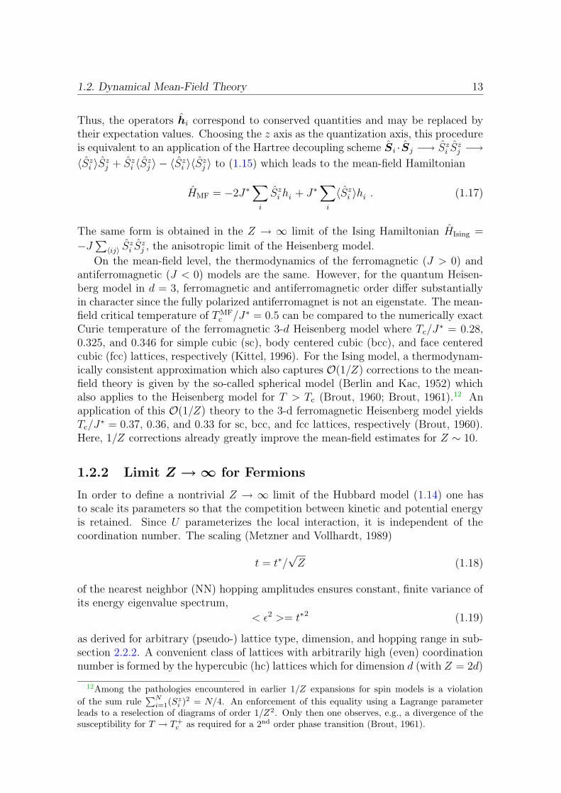
1.2. Dynamical Mean-Field Theory 13
Thus, the operators hi correspond to conserved quantities and may be replaced bytheir expectation values. Choosing the z axis as the quantization axis, this procedureis equivalent to an application of the Hartree decoupling scheme Si ·Sj −→ Szi S
zj −→
〈Szi 〉Szj + Szi 〈Szj 〉 − 〈Szi 〉〈Szj 〉 to (1.15) which leads to the mean-field Hamiltonian
HMF = −2J∗∑
i
Szi hi + J∗∑
i
〈Szi 〉hi . (1.17)
The same form is obtained in the Z → ∞ limit of the Ising Hamiltonian HIsing =
−J∑
〈ij〉 Szi S
zj , the anisotropic limit of the Heisenberg model.
On the mean-field level, the thermodynamics of the ferromagnetic (J > 0) andantiferromagnetic (J < 0) models are the same. However, for the quantum Heisen-berg model in d = 3, ferromagnetic and antiferromagnetic order differ substantiallyin character since the fully polarized antiferromagnet is not an eigenstate. The mean-field critical temperature of TMF
c /J∗ = 0.5 can be compared to the numerically exactCurie temperature of the ferromagnetic 3-d Heisenberg model where Tc/J
∗ = 0.28,0.325, and 0.346 for simple cubic (sc), body centered cubic (bcc), and face centeredcubic (fcc) lattices, respectively (Kittel, 1996). For the Ising model, a thermodynam-ically consistent approximation which also captures O(1/Z) corrections to the mean-field theory is given by the so-called spherical model (Berlin and Kac, 1952) whichalso applies to the Heisenberg model for T > Tc (Brout, 1960; Brout, 1961).12 Anapplication of this O(1/Z) theory to the 3-d ferromagnetic Heisenberg model yieldsTc/J
∗ = 0.37, 0.36, and 0.33 for sc, bcc, and fcc lattices, respectively (Brout, 1960).Here, 1/Z corrections already greatly improve the mean-field estimates for Z ∼ 10.
1.2.2 Limit Z → ∞ for Fermions
In order to define a nontrivial Z → ∞ limit of the Hubbard model (1.14) one hasto scale its parameters so that the competition between kinetic and potential energyis retained. Since U parameterizes the local interaction, it is independent of thecoordination number. The scaling (Metzner and Vollhardt, 1989)
t = t∗/√Z (1.18)
of the nearest neighbor (NN) hopping amplitudes ensures constant, finite variance ofits energy eigenvalue spectrum,
< ε2 >= t∗2 (1.19)
as derived for arbitrary (pseudo-) lattice type, dimension, and hopping range in sub-section 2.2.2. A convenient class of lattices with arbitrarily high (even) coordinationnumber is formed by the hypercubic (hc) lattices which for dimension d (with Z = 2d)
12Among the pathologies encountered in earlier 1/Z expansions for spin models is a violation
of the sum rule∑N
i=1(Szi )2 = N/4. An enforcement of this equality using a Lagrange parameter
leads to a reselection of diagrams of order 1/Z2. Only then one observes, e.g., a divergence of thesusceptibility for T → T+
c as required for a 2nd order phase transition (Brout, 1961).
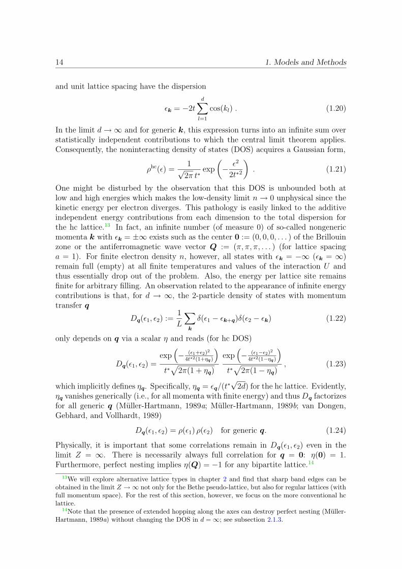
14 1. Models and Methods
and unit lattice spacing have the dispersion
εk = −2td∑
l=1
cos(kl) . (1.20)
In the limit d→∞ and for generic k, this expression turns into an infinite sum overstatistically independent contributions to which the central limit theorem applies.Consequently, the noninteracting density of states (DOS) acquires a Gaussian form,
ρhc(ε) =1√
2π t∗exp
(
− ε2
2t∗2
)
. (1.21)
One might be disturbed by the observation that this DOS is unbounded both atlow and high energies which makes the low-density limit n→ 0 unphysical since thekinetic energy per electron diverges. This pathology is easily linked to the additiveindependent energy contributions from each dimension to the total dispersion forthe hc lattice.13 In fact, an infinite number (of measure 0) of so-called nongenericmomenta k with εk = ±∞ exists such as the center 0 := (0, 0, 0, . . . ) of the Brillouinzone or the antiferromagnetic wave vector Q := (π, π, π, . . . ) (for lattice spacinga = 1). For finite electron density n, however, all states with εk = −∞ (εk = ∞)remain full (empty) at all finite temperatures and values of the interaction U andthus essentially drop out of the problem. Also, the energy per lattice site remainsfinite for arbitrary filling. An observation related to the appearance of infinite energycontributions is that, for d → ∞, the 2-particle density of states with momentumtransfer q
Dq(ε1, ε2) :=1
L
∑
k
δ(ε1 − εk+q)δ(ε2 − εk) (1.22)
only depends on q via a scalar η and reads (for hc DOS)
Dq(ε1, ε2) =exp
(
− (ε1+ε2)2
4t∗2(1+ηq)
)
t∗√
2π(1 + ηq)
exp(
− (ε1−ε2)2
4t∗2(1−ηq)
)
t∗√
2π(1− ηq), (1.23)
which implicitly defines ηq. Specifically, ηq = εq/(t∗√2d) for the hc lattice. Evidently,
ηq vanishes generically (i.e., for all momenta with finite energy) and thusDq factorizesfor all generic q (Muller-Hartmann, 1989a; Muller-Hartmann, 1989b; van Dongen,Gebhard, and Vollhardt, 1989)
Dq(ε1, ε2) = ρ(ε1) ρ(ε2) for generic q. (1.24)
Physically, it is important that some correlations remain in Dq(ε1, ε2) even in thelimit Z = ∞. There is necessarily always full correlation for q = 0: η(0) = 1.Furthermore, perfect nesting implies η(Q) = −1 for any bipartite lattice.14
13We will explore alternative lattice types in chapter 2 and find that sharp band edges can beobtained in the limit Z →∞ not only for the Bethe pseudo-lattice, but also for regular lattices (withfull momentum space). For the rest of this section, however, we focus on the more conventional hclattice.
14Note that the presence of extended hopping along the axes can destroy perfect nesting (Muller-Hartmann, 1989a) without changing the DOS in d =∞; see subsection 2.1.3.
1.2. Dynamical Mean-Field Theory 15
Little is usually said in the literature about the distribution of nongeneric mo-menta and the topology of Fermi surfaces in high dimensions. Even Gebhard’s (1997)motivation for the random dispersion approximation (RDA, see below) which is basedon the generic factorization (1.24) of the 2-particle DOS is somewhat vague andpartially incorrect in this respect. In App. A.2, we attempt a more careful charac-terization of generic and nongeneric momenta. While the modifications relative toGebhard’s view do not explain the discrepancy between RDA result and all recentDMFT results for the MIT (see chapter 3), they shed more light on foundations ofthe DMFT which will prove useful for our development of a generalized dispersionformalism in Sec. 2.3.
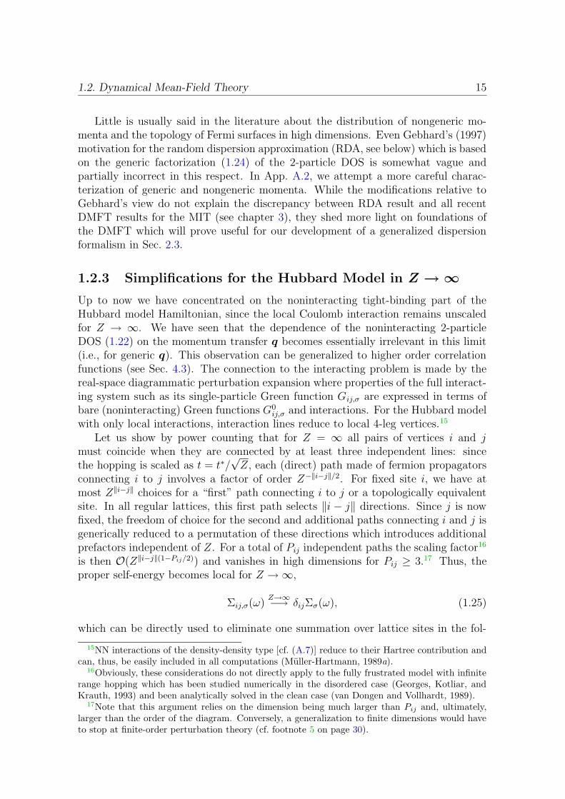
1.2.3 Simplifications for the Hubbard Model in Z → ∞
Up to now we have concentrated on the noninteracting tight-binding part of theHubbard model Hamiltonian, since the local Coulomb interaction remains unscaledfor Z → ∞. We have seen that the dependence of the noninteracting 2-particleDOS (1.22) on the momentum transfer q becomes essentially irrelevant in this limit(i.e., for generic q). This observation can be generalized to higher order correlationfunctions (see Sec. 4.3). The connection to the interacting problem is made by thereal-space diagrammatic perturbation expansion where properties of the full interact-ing system such as its single-particle Green function Gij,σ are expressed in terms ofbare (noninteracting) Green functions G0
ij,σ and interactions. For the Hubbard modelwith only local interactions, interaction lines reduce to local 4-leg vertices.15
Let us show by power counting that for Z = ∞ all pairs of vertices i and jmust coincide when they are connected by at least three independent lines: sincethe hopping is scaled as t = t∗/
√Z, each (direct) path made of fermion propagators
connecting i to j involves a factor of order Z−||i−j||/2. For fixed site i, we have atmost Z ||i−j|| choices for a “first” path connecting i to j or a topologically equivalentsite. In all regular lattices, this first path selects ||i − j|| directions. Since j is nowfixed, the freedom of choice for the second and additional paths connecting i and j isgenerically reduced to a permutation of these directions which introduces additionalprefactors independent of Z. For a total of Pij independent paths the scaling factor16
is then O(Z ||i−j||(1−Pij/2)) and vanishes in high dimensions for Pij ≥ 3.17 Thus, theproper self-energy becomes local for Z →∞,
Σij,σ(ω)Z→∞−→ δijΣσ(ω), (1.25)
which can be directly used to eliminate one summation over lattice sites in the fol-
15NN interactions of the density-density type [cf. (A.7)] reduce to their Hartree contribution andcan, thus, be easily included in all computations (Muller-Hartmann, 1989a).
16Obviously, these considerations do not directly apply to the fully frustrated model with infiniterange hopping which has been studied numerically in the disordered case (Georges, Kotliar, andKrauth, 1993) and been analytically solved in the clean case (van Dongen and Vollhardt, 1989).
17Note that this argument relies on the dimension being much larger than Pij and, ultimately,larger than the order of the diagram. Conversely, a generalization to finite dimensions would haveto stop at finite-order perturbation theory (cf. footnote 5 on page 30).

16 1. Models and Methods
lowing general real-space Dyson equation (for a time-invariant system),
Gij,σ(ω) = G0ij,σ(ω) +
∑
kl
G0ik,σ(ω)Σkl,σ(ω)Glj,σ(ω) . (1.26)
This is also the defining equation for the proper self-energy.18 For translationallyinvariant systems one can simplify this equation by Fourier transformation,
G−1σ (k, ω) = (G0
σ(k, ω))−1 − Σ(k, ω); Σ(k, ω) ≡ Σ(ω) . (1.27)
Consequently, the local Green function can be expressed in terms of the noninteract-ing DOS and the self-energy alone,
Gσ(ω) ≡ Gii,σ(ω) =1
VB
∑
k
1
ω + µ− εk − Σσ(ω)(1.28)
=
∞∫
−∞
dερ(ε)
ω + µ− ε− Σσ(ω). (1.29)
An alternative derivation of the q-independence of the proper self-energy is basedon the observation that the Laue function δ∗(q) =
∑
K δ(q + K) (with reciprocallattice vectors K) becomes effectively momentum-independent when applied to theinternal vertices of a diagram (such as a vertex of the inserted proper self-energy).Thus, the self-energy cannot depend on the external momentum and is consequentlymomentum-independent (Muller-Hartmann, 1989a).
The absence of momentum dependence in the self-energy greatly simplifies thetreatment of the Hubbard model. One may, in fact, single out one of the lattice sitesand replace the influence of its neighbors by the interaction with a single, frequency-dependent bath, i.e., map the Hubbard model onto a single impurity Anderson model(SIAM) in the limit Z → ∞. In order to restore the periodicity of the originallattice, this medium has to be determined self-consistently (Jarrell, 1992; Georges andKotliar, 1992; Janis and Vollhardt, 1992; Georges, Kotliar, Krauth, and Rozenberg,1996). Written in terms of fermionic Matsubara frequencies19 ωn = (2n + 1)πT ,self-energy Σσn ≡ Σσ(iωn), and Green function Gσn ≡ Gσ(iωn) the resulting coupledequations read
Gσn =
∞∫
−∞
dερ(ε)
iωn + µ− Σσn − ε(1.30)
Gσn = −〈ψσnψ∗σn〉A. (1.31)
18A self-energy is called proper if its external vertices cannot be be separated by cutting a singleGreen function line which implies that they are connected by at least three such lines.
19We here chose an imaginary-time formulation for brevity and in anticipation of its use in thecontext of the imaginary-time quantum Monte Carlo algorithm discussed in Sec. 1.3.
1.2. Dynamical Mean-Field Theory 17
−int. Dyson eq.k
Σ
G
G
impurity problem
G
Σ0
(1.30)
(1.35)
(1.31)
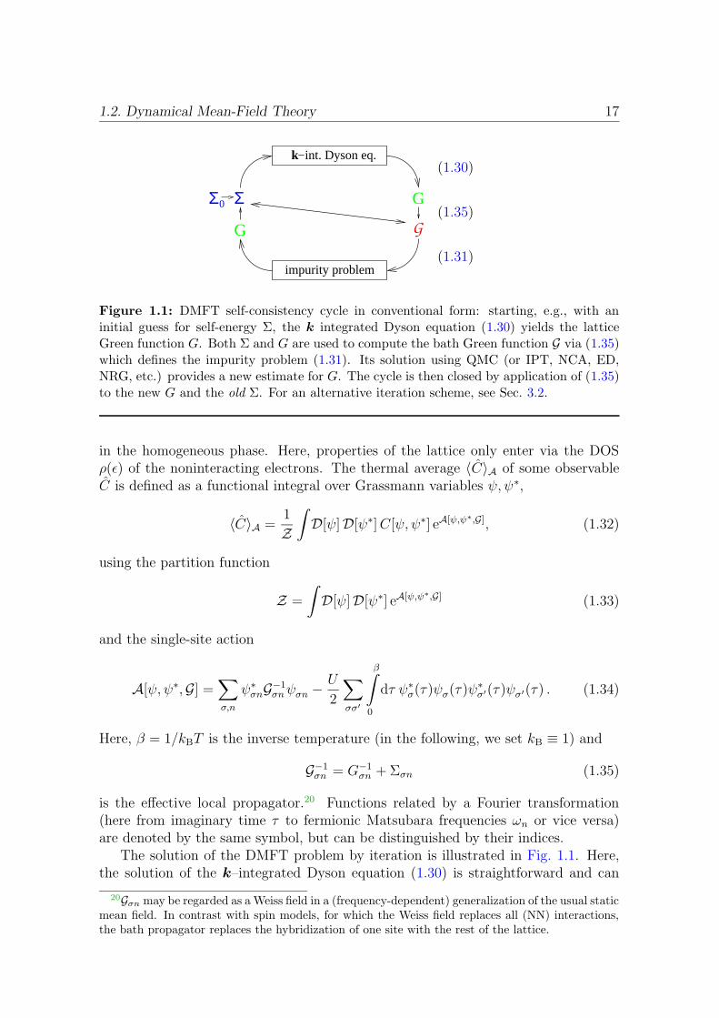
Figure 1.1: DMFT self-consistency cycle in conventional form: starting, e.g., with aninitial guess for self-energy Σ, the k integrated Dyson equation (1.30) yields the latticeGreen function G. Both Σ and G are used to compute the bath Green function G via (1.35)which defines the impurity problem (1.31). Its solution using QMC (or IPT, NCA, ED,NRG, etc.) provides a new estimate for G. The cycle is then closed by application of (1.35)to the new G and the old Σ. For an alternative iteration scheme, see Sec. 3.2.
in the homogeneous phase. Here, properties of the lattice only enter via the DOSρ(ε) of the noninteracting electrons. The thermal average 〈C〉A of some observableC is defined as a functional integral over Grassmann variables ψ, ψ∗,
〈C〉A =1
Z
∫
D[ψ]D[ψ∗]C[ψ, ψ∗] eA[ψ,ψ∗,G], (1.32)
using the partition function
Z =
∫
D[ψ]D[ψ∗] eA[ψ,ψ∗,G] (1.33)
and the single-site action
A[ψ, ψ∗,G] =∑
σ,n
ψ∗σnG−1
σnψσn −U
2
∑
σσ′
β∫
0
dτ ψ∗σ(τ)ψσ(τ)ψ
∗σ′(τ)ψσ′(τ) . (1.34)
Here, β = 1/kBT is the inverse temperature (in the following, we set kB ≡ 1) and
G−1σn = G−1
σn + Σσn (1.35)
is the effective local propagator.20 Functions related by a Fourier transformation(here from imaginary time τ to fermionic Matsubara frequencies ωn or vice versa)are denoted by the same symbol, but can be distinguished by their indices.
The solution of the DMFT problem by iteration is illustrated in Fig. 1.1. Here,the solution of the k–integrated Dyson equation (1.30) is straightforward and can
20Gσn may be regarded as a Weiss field in a (frequency-dependent) generalization of the usual staticmean field. In contrast with spin models, for which the Weiss field replaces all (NN) interactions,the bath propagator replaces the hybridization of one site with the rest of the lattice.

18 1. Models and Methods
be performed analytically for the semi-elliptic Bethe DOS (see Sec. 2.2) used inchapter 3. In contrast, the solution of the impurity problem (1.31) is highly non-trivial.21 Most numerical methods developed for the treatment of SIAMs with fixedbath could be adapted to the DMFT problem, e.g., solutions based on exact di-agonalization (ED) (Caffarel and Krauth, 1994; Georges et al., 1996), the non-crossing approximation (NCA) (Keiter and Kimball, 1970; Bickers, Cox, and Wilkins,1987; Pruschke and Grewe, 1989; Pruschke, Cox, and Jarrell, 1993), the fluctuation-exchange approximation (FLEX) (Bickers, Scalapino, and White, 1989; Bickers andScalapino, 1989; Bickers and White, 1991), the numerical renormalization group(NRG) (Wilson, 1975; Krishna-murthy, Wilkins, and Wilson, 1980; Costi, Hewson,and Zlatic, 1994; Bulla, 2000), and quantum Monte Carlo (QMC) algorithms. Wewill introduce the QMC method in Sec. 1.3 and use it throughout the numericalparts of this work; we will later also compare to results obtained from the othermethods mentioned above as well as from iterated perturbation theory (IPT), whichfor half-filling (n = 1) is based on the following second-order approximation for theself-energy (Georges and Kotliar, 1992),
ΣIPTσn =
U
2+ U 2
β∫
0
dτ eiωnτ(Gσ(τ)
)3; Gσ(τ) = Gσ(τ)−
U
2(1.36)
and becomes exact both at weak and strong coupling (Zhang, Rozenberg, and Kotliar,1993).
While the DMFT is a very successful theory for correlated electron systems due toits nonperturbative character, it misses some important physics even in three dimen-sions and may fail completely for two dimensional systems. In particular, phenom-ena which involve strong momentum dependence such as d-wave superconductivitycannot be described within the DMFT. Attempts to build up a more widely ap-plicable theory by systematically including O(1/Z) corrections have failed so far toproduce breakthroughs for finite-dimensional systems (Gebhard, 1990; Vlaming andVollhardt, 1992; van Dongen, 1994c; Schiller and Ingersent, 1995; Pruschke, Metzner,and Vollhardt, 2001).22 However, significant progress has been made recently usingschemes which interpolate between the DMFT single impurity problem and finite-dimensional clusters (with periodic boundary conditions). These fascinating exten-sions of the DMFT, namely the DCA and the CDMFT are reviewed in App. A.3,together with the RDA which was constructed as an alternative to the DMFT self-consistency approach.
21An exception is the application of (1.30) and (1.31) to a Lorentzian DOS ρ(ε) = t/(π(ε2 + t2))which can be realized on lattices with long range hopping (Georges and Kotliar, 1992). For thisDOS (which is clearly pathological due to its infinite variance), the Weiss function is independentof U ; furthermore (1.31) is solvable by Bethe ansatz in this case so that many properties can beobtained analytically.
22Recently, an improved version of the Schiller-Ingersent scheme was applied for the hypercubiclattice using the FLEX approximation. Although no violation of causality was observed in this case,the causality of the method in general is still unclear (Zarand, Cox, and Schiller, 2000).
1.3. Quantum Monte Carlo Algorithm 19
1.3 Quantum Monte Carlo Algorithm
In this section, we will discuss the auxiliary-field quantum Monte Carlo (QMC) al-gorithm used in this work for solving the impurity model (1.31). It was originallyformulated for treating a small number of magnetic impurities in metals (Hirsch andFye, 1986) and later applied to arbitrary hybridization functions, i.e., in the form re-quired for the solution of the DMFT problem (Jarrell, 1992; Rozenberg, Zhang, andKotliar, 1992; Georges and Krauth, 1992; Ulmke, Janis, and Vollhardt, 1995). Beforewe discuss technical details, let us point out some general important consequences ofusing this particular method for solving the impurity problem: First of all, the QMCmethod is formulated in imaginary time, i.e., G(τ) is evaluated (as a functional ofG(τ) and the model parameters) which implies that dynamical information can beobtained directly only for imaginary Matsubara frequencies and that analytic con-tinuation is required for getting information, e.g., the spectrum, at real frequencies(see Sec. 1.4). A second implication is that Fourier transforms are necessary in orderto connect the imaginary-time impurity part with the Dyson equations (1.30) and(1.35) which are diagonal in frequency space. Finally, the QMC method introducesa discretization ∆τ of the imaginary time β which not only necessitates an extra-polation of all DMFT(QMC) results to the physical limit ∆τ → 0 (using convergedDMFT solutions for different values of ∆τ) and restricts the method to relativelyhigh temperatures, but also complicates the Fourier transformations. Here, we willconcentrate on the solution of the impurity problem and discuss problems related tothe Fourier transforms in Sec. 3.4. We also specialize to the single-band homogeneouscase; for the generalization to the multi-band cases used in chapter 5, we refer to theliterature (Rozenberg, 1997; Han, Jarrell, and Cox, 1998; Held and Vollhardt, 1998).
1.3.1 Wick’s Theorem for the Discretized Impurity Problem
The difficulty in solving the functional integral equation (1.31) arises from the non-commutativity of the kinetic term and the interaction term in the single-site ac-tion (1.34). These terms can be separated by use of the Trotter-Suzuki formula(Trotter, 1959; Suzuki, 1976) for operators A and B:
e−β(A+B) =(e−∆τA e−∆τB
)Λ+O(∆τ) , (1.37)
where ∆τ = β/Λ and Λ is the number of (imaginary) time slices.23 Rewriting theaction (1.34) in discretized form
AΛ[ψ, ψ∗,G, U ] = (∆τ)2∑
σ
Λ−1∑
l,l′=0
ψ∗σl(G
−1σ )ll′ ψσl′
−∆τUΛ−1∑
l=0
ψ∗↑l ψ↑l ψ
∗↓l ψ↓l, (1.38)
23Since β = 1/kBT is the inverse temperature, small ∆τ on each “time slice” corresponds to ahigher temperature, for which the operators effectively decouple. Thus, we may view the Trotterapproach as a numerical extension of a high-temperature expansion to lower temperatures.

20 1. Models and Methods
where the matrix Gσ consists of elements Gσll′ ≡ Gσ(l∆τ − l′∆τ), we apply (1.37)and obtain to lowest order
exp (AΛ[ψ, ψ∗,G, U ]) =Λ−1∏
l=0
[
exp(
(∆τ)2∑
σ
Λ−1∑
l′=0
ψ∗σl(G
−1σ )ll′ ψσl′
)
× exp(−∆τ U ψ∗
↑l ψ↑l ψ∗↓l ψ↓l
)]
. (1.39)
Shifting the chemical potential by U/2, the four-fermion term can be rewritten asa square of two-fermion terms, which makes it suitable for the following discreteHubbard-Stratonovich transformation (Hirsch, 1983):
exp
(∆τU
2(ψ∗
↑l ψ↑l − ψ∗↓l ψ↓l)
2
)
=1
2
∑
sl =±1
exp(λsl(ψ
∗↑l ψ↑l − ψ∗
↓l ψ↓l))
(1.40)
with coshλ = exp(∆τU/2). Here, the interaction between electrons is replaced bythe interaction with an auxiliary binary field s with components sl for 0 ≤ l ≤ Λ.Acting like a local, but time-dependent magnetic field, s can be regarded as anensemble of Ising spins.
These transformations yield an expression for the functional integral
Gσl1l2 =1
Z∑
s
∫
D[ψ]D[ψ∗] ψ∗σl1ψσl2 exp
(∑
σ,l,l′
ψ∗σlM
sl
σll′ψσl′)
, (1.41)
with24
M sl
σll′ = (∆τ)2(G−1σ )ll′ − λσδll′sl, (1.42)
where in (1.41) the sum is taken over all configurations of the Ising spin field, andeach term of the sum involves independent fermions only. Now Wick’s theorem (see,e.g., Negele and Orland, 1987) can be applied to get the solution
Gσll′ =1
Z∑
s
(M s
σ
)−1
ll′det M
s↑ det M
s↓ , (1.43)
where Msσ is the matrix with elements M sl
σll′ , and the partition function has thevalue
Z =∑
sdet M
s↑ det M
s↓ . (1.44)
Computing one of the 2Λ terms in (1.43) directly from definition (1.42) is an operationof order O(Λ3). If the terms are ordered in a way so that successive configurations sand s′ only differ by one flipped spin sl → −sl then all matrices and determinantscan be updated at a cost of O(Λ2) (Blankenbecler, Scalapino, and Sugar, 1981). Onlyfor Λ . 24 can all terms be summed up exactly. Computations at larger Λ are madepossible by Monte Carlo importance sampling which reduces the number of termsthat have to be calculated explicitly from 2Λ to order O(Λ).
24A more precise form including subleading corrections is M sl
σll′ = (∆τ)2 (G−1σ )ll′ eλσsl′ + δll′
(1−
eλσsl)
(Held, 1999; Georges et al., 1996).
1.3. Quantum Monte Carlo Algorithm 21
1.3.2 Monte Carlo Importance Sampling
Monte Carlo (MC) procedures in general are stochastic methods for estimating largesums (or high-dimensional integrals) by picking out a comparatively small numberof terms (or evaluating the integrand only for a relatively small number of points).Let us assume we want to compute the average X := 1
M
∑Ml=1 xl, where l is an index
(e.g., an Ising configuration l ≡ s) and x some observable with the (true) variancevx = 1
M
∑Ml=1(xl−X)2. In a simple MC approach (as used, e.g., for the computation
of densities of states in chapter 2), one may select a subset of N ¿ M indicesindependently with a uniform random distribution P (lj) = const. (for 1 ≤ j ≤ N),
(XMC
)2=
1
N
N∑
j=1
xlj (1.45)
∆XMC := 〈(XMC −X)2〉 =vxN≈ 1
N(N − 1)
N∑
j=1
(xlj −XMC)2 . (1.46)
Here, the averages are taken over all realizations of the random experiment (eachconsisting of a selection of N indices). In the limit of N → ∞, the distribution ofXMC becomes Gaussian according to the central limit theorem. Only in this limit isthe estimate of vx from the QMC data reliable.
Smaller errors and faster convergence to a Gaussian distribution for the estimatemay be obtained by importance sampling. Here, the function xl is split up,
xl = pl ol; pl ≥ 0;M∑
l=1
pl = c , (1.47)
where we may regard pl as a (unnormalized) probability distribution for the indicesand ol as a remaining observable. If both the normalization c is known (i.e, thesum over the weights pl can be performed exactly) and the corresponding probabilitydistribution can be realized (by drawing indices l with probability P (l) = pl/c), weobtain
XMCimp =
c
N
N∑
j=1
olj and ∆XMCimp = c
√voN. (1.48)
Thus, the error can be reduced (vo < c2vx), when the problem is partially solvable, i.e.,the sum over pl with pl ≈ xl can be computed.25 Since this is not possible in general,one usually has to treat the normalization c as an unknown and realize the probabilitydistribution P (lj) = plj/c in a stochastic Markov process: Starting with some initialconfiguration l1, a chain of configurations is built up where in each step only a smallsubset of configurations l′ is accessible in a “transition” from configuration l. Providedthat the transition rules satisfy the detailed balance principle,
pl P(l → l′) = pl′ P(l′ → l) , (1.49)
25The possible reduction of the variance is limited when xl is of varying sign. This “minus-signproblem” seriously restricts the applicability of Monte Carlo methods for finite-dimensional fermionproblems.

22 1. Models and Methods
and the process is ergodic (i.e., all configurations can be reached from some startingconfiguration), the distribution of configurations of the chain approaches the targetdistribution in the limit of infinite chain length. Since the normalization remainsunknown, importance sampling by a Markov process can only yield ratios of differentobservables evaluated on the same chain of configurations. Another consequenceof using a Markov process is that initial configurations have to be excluded fromaverages since the true associated probabilities might be vanishingly small. Theywould otherwise be overrepresented in any run of finite length. Consequently, we willlater distinguish “warmup sweeps” from “measurement sweeps”.
For the computation of errors, one has to take into account the finite autocor-relation induced by the Markov process, i.e., correlation between subsequent mea-surements. This correlaton may be characterized by the autocorrelation time26
κo ≥ 1 which effectively reduces the number of independent samples, so that ∆X =c√
voκo/N . The numerical effort necessary to reach some target statistical accuracy∆X nevertheless increases only as (1/∆X)2.
Returning to the evaluation of the Green function using (1.43) and (1.44), theobvious choice is to sample configurations s according to the (unnormalized) prob-ability
P (s) =∣∣∣ det M
s↑ det M
s↓
∣∣∣ . (1.50)
The Green function can then be calculated as an average 〈. . . 〉s over these configu-rations:
Gσll′ =1
Z
⟨(M s
σ
)−1
ll′sign
(
det Ms↑ det M
s↓
)⟩
s, (1.51)
Z =⟨
sign(
det Ms↑ det M
s↓
)⟩
s. (1.52)
Here, Z deviates from the full partition function by an unknown prefactor whichcancels in (1.51). The inability to compute the partition function is a consequence ofthe importance sampling and is thus a general characteristic of QMC methods. Thiswill have severe consequences for the study of phase transitions (see chapter 3).
In this work, the transition probability is chosen according to the Metropolistransition rule (Metropolis, Rosenbluth, Rosenbluth, Teller, and Teller, 1953)27
P(x→ y) = min1, P (y)/P (z) (1.53)
for transitions from a spin configuration x to a configuration y, which clearly fulfillsdetailed balance (1.49). Configuration updates are always performed by sweeping
26For a set o1, o2, . . . , oN of measurements, the autocorrelation function (for the observableo) is col = 〈(ok − 〈o〉)(ok+l − 〈o〉)〉k. An associated autocorrelation time may then be defined as
κo = co0 + 2∑N0
l=1 col , where the cutoff N0 is determined by col > 0 for l ≤ N0 and cN0+1 < 0.
27Since in the present problem most of the computational cost is associated with the spin updateand only has to be paid for accepted spin flips, the Metropolis rule, which has the highest acceptanceratio compatible with detailed balance, might not be optimal. Our tests with the symmetric heat-bath rule and generalizations of it which further suppress transitions between states with similarprobability did not, however, lead to significant saving of computer time at constant accuracy.

1.4. Maximum Entropy Method 23
through the full spin field, i.e., by attempting to flip spins s0 through sΛ−1 one afterthe other and then starting the next sweep. Roughly, the number of such sweepshas to be held constant (rather than the number of attempted single-spin flips) forconstant statistical error when the number of spins Λ is varied. Since the systematicerror depends on ∆τ , the necessary number of time slices is proportional to theinverse temperature, Λ ∝ β, so that the total numerical cost for given accuracy isproportional to β3.
In this work, up to Λ = 400 time slices and up to 107 measurement sweeps wereused. A single iteration for Λ = 400 with 200000 sweeps took more than 7 CPUhours on a Cray T90. Since typically 10-20 iterations are needed for well-convergedsolutions (even when initializing the runs with data obtained for larger ∆τ), thecomputation of each such data point took several weeks of real time and used upabout a monthly contingent of supercomputer time. No minus-sign problem wasencountered, i.e., the sign in (1.51) and (1.52) was always positive.
1.4 Maximum Entropy Method
Within the DMFT, all single-particle properties can be expressed in terms of the localsingle-particle spectral function (also called “full” or “interacting” density of states)which is proportional to the imaginary part of the local retarded Green function,
A(ω) = − 1
πImG(ω + i0+) . (1.54)
The spectral function A(ω) is accessible experimentally: measured (angular aver-aged) photoemission spectra (PES) can under certain simplifying assumptions (seesubsection 5.4.1) be identified with A(ω) multiplied by the Fermi function nf(ω−µ).Correspondingly, inverse photoemission spectra or X-ray absorption spectra (XAS)can be identified with A(ω) multiplied by 1−nf(ω−µ). Furthermore, nonlocal spec-tral functions and the optical conductivity σ(ω) can, within the DMFT, be calculatedfrom A(ω) (see chapter 4).
In QMC calculations, however, the Green function G (and thus the spectral func-tion A(ω)) cannot be directly computed on the real axis. Instead, real-time dynami-cal information has to be extracted from imaginary-time data G(τ) (or, equivalently,from the Fourier transformed Matsubara-frequency data G(iωn)) via analytic contin-uation. This is in principle possible through inversion of the spectral representationfor G(τ), i.e.,
G(τ) =
∞∫
−∞
dω K(τ, ω − µ; β) A(ω) , (1.55)
K(τ, ω; β) :=exp(−τω)
1 + exp(−βω), (1.56)
but poses an ill-conditioned problem since G(τ) is only measured on a grid τl = l∆τ(where ∆τ = β/Λ) and since the kernel (1.56) becomes exponentially small for generic
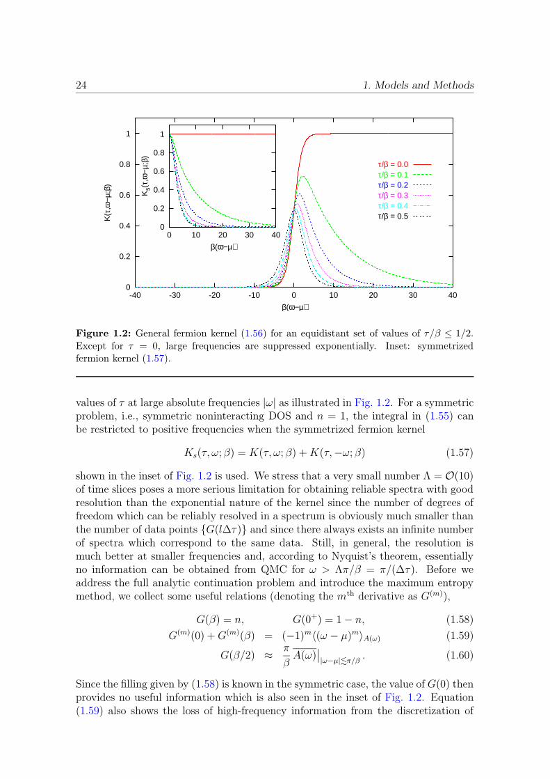
24 1. Models and Methods
0
0.2
0.4
0.6
0.8
1
-40 -30 -20 -10 0 10 20 30 40
K(τ
,ω−µ
;β)
β(ω−µ)
τ/β = 0.0τ/β = 0.1τ/β = 0.2τ/β = 0.3τ/β = 0.4τ/β = 0.5
0
0.2
0.4
0.6
0.8
1
0 10 20 30 40
Ks(
τ,ω
−µ;β
)
β(ω−µ)
Figure 1.2: General fermion kernel (1.56) for an equidistant set of values of τ/β ≤ 1/2.Except for τ = 0, large frequencies are suppressed exponentially. Inset: symmetrizedfermion kernel (1.57).
values of τ at large absolute frequencies |ω| as illustrated in Fig. 1.2. For a symmetricproblem, i.e., symmetric noninteracting DOS and n = 1, the integral in (1.55) canbe restricted to positive frequencies when the symmetrized fermion kernel
Ks(τ, ω; β) = K(τ, ω; β) +K(τ,−ω; β) (1.57)
shown in the inset of Fig. 1.2 is used. We stress that a very small number Λ = O(10)of time slices poses a more serious limitation for obtaining reliable spectra with goodresolution than the exponential nature of the kernel since the number of degrees offreedom which can be reliably resolved in a spectrum is obviously much smaller thanthe number of data points G(l∆τ) and since there always exists an infinite numberof spectra which correspond to the same data. Still, in general, the resolution ismuch better at smaller frequencies and, according to Nyquist’s theorem, essentiallyno information can be obtained from QMC for ω > Λπ/β = π/(∆τ). Before weaddress the full analytic continuation problem and introduce the maximum entropymethod, we collect some useful relations (denoting the mth derivative as G(m)),
G(β) = n, G(0+) = 1− n, (1.58)
G(m)(0) +G(m)(β) = (−1)m〈(ω − µ)m〉A(ω) (1.59)
G(β/2) ≈ π
βA(ω)
∣∣|ω−µ|.π/β . (1.60)
Since the filling given by (1.58) is known in the symmetric case, the value of G(0) thenprovides no useful information which is also seen in the inset of Fig. 1.2. Equation(1.59) also shows the loss of high-frequency information from the discretization of
1.4. Maximum Entropy Method 25
imaginary time: for a finite grid the error in estimating derivatives G(m) increasesrapidly with order m; thus, the determination of high order moments 〈(ω− µ)m〉A(ω)
of the spectrum is in general an ill-posed problem. At low temperatures, G(β/2)gives a hint as to the weight of a quasiparticle peak or the existence of a gap via(1.60) since its value is proportional to the value of the spectral function near theFermi energy, averaged over an inverse hyperbolic cosine with width π/β.
First attempts to address the analytic continuation problem for QMC data in-cluded least-squares fits, Pade approximants, and regularization (for references, seethe pedagogical and concise review by Jarrell (1997)). Least-squares fits of spectraapproximated as a set of box functions are inherently unstable. Pade approximationsfor G(iωn) only work well for very precise data (e.g., in the context of Eliashbergequations), but not for QMC. Regularization of the kernel (1.56) tends to produceoverly smeared-out spectra. What is needed instead is a regularization of the solutionA(ω) that only shows features which are supported by the data, but is as smoothas possible otherwise. This is essentially the idea of the maximum entropy method(MEM) of finding the most probable spectrum compatible with the data.
The MEM is a very general approach for reconstructing continuous, positivesemidefinite functions (i.e., densities or spectra) from incomplete, noisy, and pos-sibly oversampled28 data. It has a long history in the context of image reconstructionin such diverse disciplines as radio aperture synthesis, optical deconvolution, X-rayimaging, structural molecular biology, and medical tomography (see Skilling andBryan (1984) and references therein). A preliminary study of its usefulness in thecontext of the analytic continuation problem (Silver, Sivia, and Gubernatis, 1990)was soon followed by applications to spectra (Silver, Gubernatis, Sivia, and Jar-rell, 1990; Jarrell, Sivia, and Patton, 1990) and correlation functions (Deisz, Jarrell,and Cox, 1990). An efficient and general formulation of a MEM algorithm for analyticcontinuation of (oversampled) QMC data was then given by Gubernatis, Jarrell, Sil-ver, and Sivia (1991), closely following the general state-of-the-art approach by Bryan(1990).
For simplicity, we will first assume that the QMC simulation produces Nd mea-surements of the observables Gl ≡ G(l∆τ), 0 ≤ l < Λ which are independent bothin computer time and in imaginary time, i.e., without significant autocorrelationbetween subsequent measurements or between adjacent imaginary time slices.29 Ifwe further disregard systematic errors and assume some “true” spectrum A [whichcorresponds to a discretized Green function Gl via (1.55)] as well as a Gaussian dis-tribution of statistical errors, the probability distribution for the observed averaged
28Data is called oversampled when measurements of different data points (here: for different τ)are not statistically independent, but correlated (Bryan, 1990). In this case, the number of “good”degrees of freedom (entering the error statistics) is reduced.
29Typically, one of the “measurements” of a set Gl is generated by binning a macroscopicnumber of measurements within QMC. Autocorrelation in computer time, i.e., between differentbins vanishes in the limit of infinite bin size.
26 1. Models and Methods
values G ≡ Gl (where Gl =∑Nd
i=1Gil) is
P (G|A) ∝ e−12χ2
; χ2 =Λ−1∑
l=0
(Gl −Gl
)2
σ2l
. (1.61)
Here, σl can be estimated from the data alone, σ2l ≈
∑Nd
i=1
(Gl − Gi
l
)2/(Nd(Nd− 1)).
Obviously, the likelihood function P (G|A) is not directly helpful; in order to find themost probable spectrum given the measured data, we need the converse probabilityP (A|G). These probabilities are related by Bayes’ theorem,
P (A|G)P (G) = P (G|A)P (A) . (1.62)
Since the data G is constant in the search for an optimal A, the associated proba-bility P (G) drops out of the problem. For the probability P (A) of a spectrum A(ω)in absence of data, an entropic ansatz is made where prior knowledge can also beincorporated by choosing an appropriate (positive semidefinite) default model m(ω),
P (A) = eαS[A(ω),m(ω)] . (1.63)
Here, α is a numerical parameter while S is a generalized Shannon-Jaynes entropy,
S[A,m] =
∫
dω(
A(ω)−m(ω)− A(ω) ln(A(ω)/m(ω)
))
. (1.64)
For a constant default model (within some finite frequency range), the entropic form(1.64) clearly favors smooth spectra. This is also true for a general smooth defaultmodel. It also enforces positivity of A and pushes the solution towards the (normal-ized) default model in absence of data. From (1.61), (1.62), and (1.63), the posteriorprobability can be read off as
P (A|G,m, α) = eαS[A,m]− 12χ2[G,A] . (1.65)
The balance between a tight match of data and a high entropy is calibrated bythe Lagrange parameter α which may be chosen so that χ2 = Λ (historic MEM).Alternatively, one may use the value of α with the highest probability P (α|G, A,m)which can approximately be calculated within the method (classic MEM). Giventhe QMC data, a default model, a representation of the spectrum (i.e., a possiblyinhomogeneous grid of ωj of frequencies for which A is going to be computed), anda starting guess for α, a simple MEM program thus both searches for the spectrumA(ωj) with maximum probability P (A|G,m, α) for given α using, e.g., the Newton-Raphson method and, in an outer loop, searches for the best value of α.
More advanced aspects of the MEM, in particular the breakdown of some as-sumptions made above and improved formulations are discussed in the context of theanalytic continuation of Green functions for correlated systems in subsection 3.8.1.
27
Chapter 2
Lattice and Density of States
Within the DMFT, properties of the lattice enter the computation of single-particleproperties via the “noninteracting” density of states (DOS) ρ(ε) only.1 Thus, inaddition to the Hubbard interaction U , the temperature T , and the density n, theDOS constitutes an infinite set of input parameters for the DMFT treatment ofthe Hubbard model. While some aspects of a given DOS are easily characterized(with, e.g., the variance setting the energy scale for U and T ), many of its degrees offreedom may influence physical properties of the interacting system in a complicatedway. More generally, the choice of hopping matrix elements or, equivalently, thechoice of a dispersion εk may be crucial for properties of Hubbard type models in anydimension. In most studies of the Hubbard model in dimensions d > 1, the hoppingrange has been restricted to nearest neighbors (NN) and, in some cases, next-nearestneighbors (NNN). While using only these largest hopping matrix elements is certainlya reasonable starting point, the remaining part can still be qualitatively important,in particular in high dimensions.
Three related problems motivate the studies presented in this chapter. First,up to now there has been no fully satisfactory way of treating the Hubbard modelrigorously in d = ∞. As shown in Sec. 1.2, NN hopping on the hypercubic (hc)lattice leads to a Gaussian DOS without band edges in d→∞, which is unphysicalsince in the low-density limit the energy per electron becomes infinite and because anunbounded band violates the single-band assumption of energetically well-separatedbands. Inclusion of NNN hopping not only leads to magnetic frustration and anasymmetric DOS but (for an appropriate sign of the hopping amplitudes) cures theproblem of infinite energy in the low-density limit by introducing a sharp lower bandedge in d → ∞.2 Another conventional way of establishing band edges in d = ∞is taking this limit on the Bethe lattice which yields the semi-elliptic DOS usedthroughout chapter 3. Here, problems arise from the fact that the Bethe lattice isnot a regular lattice but a treelike structure which has no loops and no well-defined
1The quotation marks, which we will drop from now on, are a reminder that (at least) interactionswith lattice ions and core electrons are already included in the “noninteracting” dispersion εk and,consequently, determine the “noninteracting” DOS.
2This cure is, however, not stable upon further extension of the hopping range: hopping tothird-nearest neighbors generically reintroduces the low-energy tail extending to ε = −∞.
28 2. Lattice and Density of States
momentum space.The second motivation for studying the relation between lattices and correspond-
ing densities of states is that the knowledge of the DOS is not sufficient for thecomputation of two-particle properties like susceptibilities and, in particular, trans-port properties. In fact, a large part of chapter 4 is devoted to the question of howthe optical conductivity σ(ω) can be defined and computed for the Bethe lattice (or,more generally, for a lattice with a semi-elliptic DOS in the limit d = ∞). It wouldbe desirable to find a regular isotropic3 and translationally invariant lattice (with awell-defined k-space) with the same single-particle properties (i.e., the same DOS)as the Bethe lattice. Transport properties could then be computed directly fromfirst principles. As shown in Sec. 2.4 and in subsection 4.4.5, this is indeed possi-ble. Another important application of the new method developed in this work is thecomputation of the optical conductivity for a given LDA DOS in Sec. 5.4. Althoughhere, in principle, the full dispersion εk could be calculated, an educated guess forthe DMFT estimate of σ(ω) will be obtained without the numerically complicatedevaluation of ∇εk.
A third point relates to the question of how relevant results calculated in d =∞are to the finite-dimensional systems of the real world. Since the DOS represents thenoninteracting limit of the model Hamiltonian in any dimension, it seems questionableto rely on features of the DOS which are not robust under change of dimensions,i.e., cannot be obtained under similar assumptions concerning the hopping matrixelements in at least any dimension 3 ≤ d ≤ ∞. One example where a feature is notgeneric although it occurs in d = 3 and d = ∞ is the singularity of the fcc DOS atthe lower band edge. This feature is not present in any finite dimension d > 3 unlessNNN hopping is chosen appropriately; see, e.g., Ulmke (1998) and Sec. 2.1. Evenmore importantly, our study of the paramagnetic Mott metal-insulator transitionperformed in chapter 3 would not be complete without a discussion of microscopicmechanisms for frustration and their implications for the DOS and for transportproperties in infinite and finite dimensions.
The numerically exact studies of tight-binding models in large but finite dimen-sions presented in this chapter were made possible by the development of a computerprogram which allows for the computation of the DOS in arbitrary (finite) dimensionsgiven the dispersion εk. This computation is performed by Monte Carlo sampling ofthe d-dimensional integral (volume VB of the Brillouin zone)
ρ(ε) =1
VB
∫
dk δ(ε− εk) (2.1)
on a discretized energy interval. Originally, the computation of the DOS was only abyproduct (at no additional cost) of computations of
ρ(ε) =1
VB
∫
dk δ(ε− εk)|vk|2 (2.2)
3Here and in the following, we use the term isotropic for a lattice with hypercubic symmetrysince in that case the cartesic axes are equivalent and all transport properties are isotropic in thelong-wavelength limit.
2.1. Hypercubic Lattice and Extensions 29
which is the essential lattice input to the optical conductivity within the bubble ap-proximation (see chapter 4 where results for ρ(ε) are also presented). However, a fastand reliable way of computing the DOS is always useful since in spite of considerableanalytic effort a numerical integration is unavoidable even for the hypercubic latticewith NN hopping in d ≥ 2 [see, e.g., Schlipf (1998)].
The most important results of this chapter are the exact analytic expression andnumerical estimates for extended hopping matrix elements defined on a hypercubiclattice which yield a semi-elliptic DOS in the limit d→∞. In fact, the new methoddeveloped in this chapter for determining dispersion, transport properties, and matrixelements in d = ∞ is very general; it can be applied for any arbitrary target DOS.The method is based on a generalization of the observation that the dispersion ofthe fcc lattice can be written as a function of the dispersion of the hc lattice. Thisexpression, a (quadratic) polynomial in εhc
k , implies a simple transformation rule forthe DOS. In the course of this thesis it became apparent that parts of the necessaryformalism had already been worked out, but had not been published. Extending vanDongen’s (2001) construction via expansion of the dispersion in Hermite polynomialswe will show that both the hopping matrix elements and all information (e.g., theFermi velocity) needed for the computation of transport properties can be obtainedin a controlled scheme.
The structure of the remainder of this chapter is as follows: In Sec. 2.1 we will firstdiscuss hypercubic lattices with NN hopping matrix elements only, then consider t-t′
hopping to NNs and NNNs and, finally, we will treat the fcc lattice which is equivalentto a hc lattice with NNN hopping only. Conventional ways of constructing a semi-elliptic DOS in d =∞, i.e., via the fractal Bethe lattice and the disordered infinite-range hopping model are summarized in Sec. 2.2. The new general dispersion schemeis then developed in Sec. 2.3. As a first practical application we use this method forthe construction of a regular lattice with Bethe semi-elliptic DOS and begin with thecharacterization of its transport properties in Sec. 2.4. The robustness of the newmethod is demonstrated by studying both the effects of truncation of the hoppingrange and of finite dimensionality. Our treatment of the hyperdiamond lattice, aregular non-Bravais lattice with a reduced number of loops, in App. B supplementsthe findings of this chapter and our discussion of loops in subsection 4.4.2.
2.1 Hypercubic Lattice and Extensions
2.1.1 Definitions and Analytical Considerations
The d-dimensional hypercubic (hc) lattice is spanned by d orthonormal primitivevectors (setting the lattice spacing to a = 1) so that the cartesian components ofeach lattice vector are integers and the Euclidean length (or 2-norm) of a vector isgiven by
|v| := ||v||2 =( d∑
α=1
v2α
)1/2
(2.3)
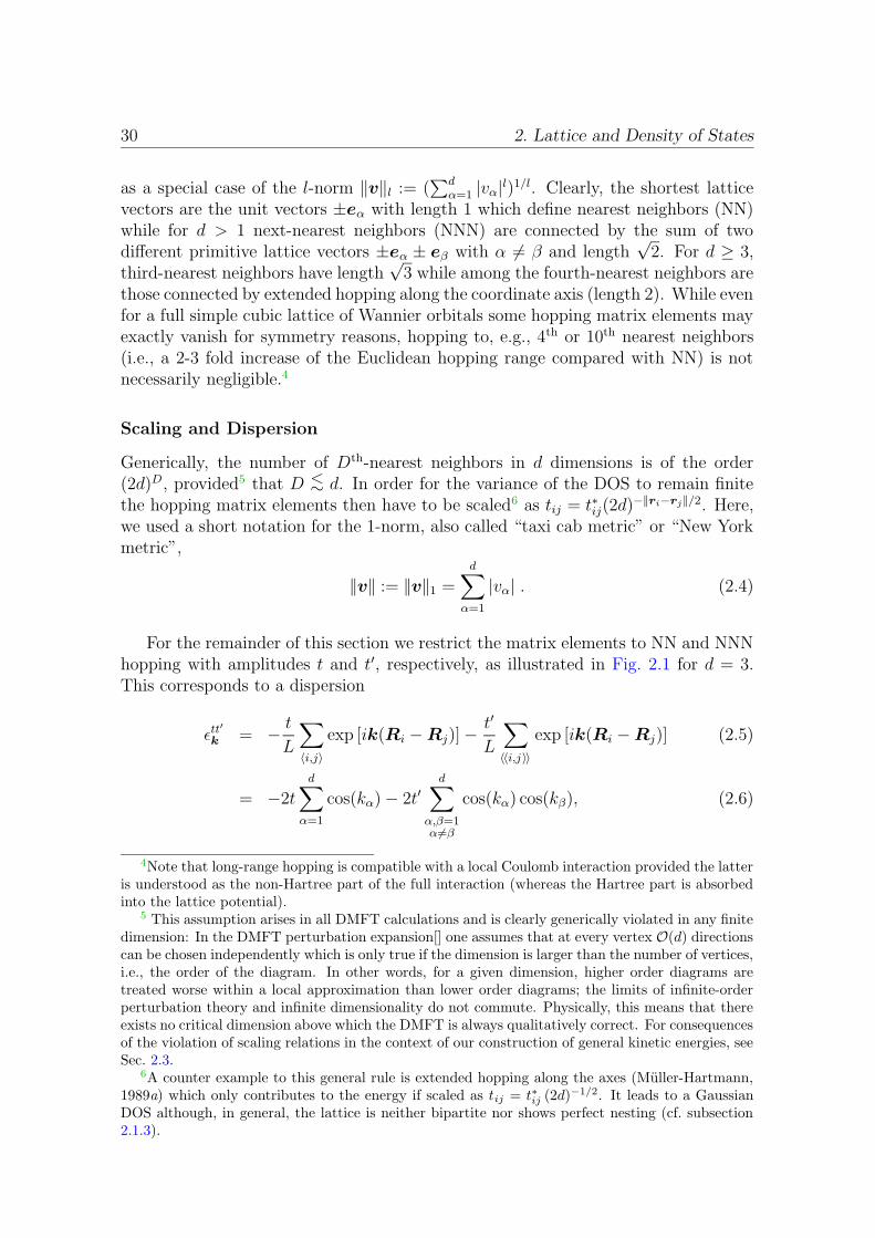
30 2. Lattice and Density of States
as a special case of the l-norm ||v||l := (∑d
α=1 |vα|l)1/l. Clearly, the shortest latticevectors are the unit vectors ±eα with length 1 which define nearest neighbors (NN)while for d > 1 next-nearest neighbors (NNN) are connected by the sum of twodifferent primitive lattice vectors ±eα ± eβ with α 6= β and length
√2. For d ≥ 3,
third-nearest neighbors have length√
3 while among the fourth-nearest neighbors arethose connected by extended hopping along the coordinate axis (length 2). While evenfor a full simple cubic lattice of Wannier orbitals some hopping matrix elements mayexactly vanish for symmetry reasons, hopping to, e.g., 4th or 10th nearest neighbors(i.e., a 2-3 fold increase of the Euclidean hopping range compared with NN) is notnecessarily negligible.4
Scaling and Dispersion
Generically, the number of Dth-nearest neighbors in d dimensions is of the order(2d)D, provided5 that D <∼ d. In order for the variance of the DOS to remain finitethe hopping matrix elements then have to be scaled6 as tij = t∗ij(2d)
−||ri−rj ||/2. Here,we used a short notation for the 1-norm, also called “taxi cab metric” or “New Yorkmetric”,
||v|| := ||v||1 =d∑
α=1
|vα| . (2.4)
For the remainder of this section we restrict the matrix elements to NN and NNNhopping with amplitudes t and t′, respectively, as illustrated in Fig. 2.1 for d = 3.This corresponds to a dispersion
εtt′
k = − tL
∑
〈i,j〉exp [ik(Ri −Rj)]−
t′
L
∑
〈〈i,j〉〉exp [ik(Ri −Rj)] (2.5)
= −2td∑
α=1
cos(kα)− 2t′d∑
α,β=1α6=β
cos(kα) cos(kβ), (2.6)
4Note that long-range hopping is compatible with a local Coulomb interaction provided the latteris understood as the non-Hartree part of the full interaction (whereas the Hartree part is absorbedinto the lattice potential).
5 This assumption arises in all DMFT calculations and is clearly generically violated in any finitedimension: In the DMFT perturbation expansion[] one assumes that at every vertex O(d) directionscan be chosen independently which is only true if the dimension is larger than the number of vertices,i.e., the order of the diagram. In other words, for a given dimension, higher order diagrams aretreated worse within a local approximation than lower order diagrams; the limits of infinite-orderperturbation theory and infinite dimensionality do not commute. Physically, this means that thereexists no critical dimension above which the DMFT is always qualitatively correct. For consequencesof the violation of scaling relations in the context of our construction of general kinetic energies, seeSec. 2.3.
6A counter example to this general rule is extended hopping along the axes (Muller-Hartmann,1989a) which only contributes to the energy if scaled as tij = t∗ij (2d)−1/2. It leads to a GaussianDOS although, in general, the lattice is neither bipartite nor shows perfect nesting (cf. subsection2.1.3).
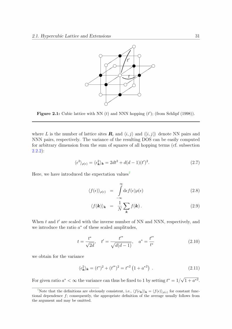
2.1. Hypercubic Lattice and Extensions 31
´´´´´´
´´´´´´
´´´
´´´
´´´
´´
´
´´´
´´
´
gw w
w
w
w
w
g g
gg
g
gg
g
g
g
g
g
t
t′
Figure 2.1: Cubic lattice with NN (t) and NNN hopping (t′); (from Schlipf (1998)).
where L is the number of lattice sites Ri and 〈i, j〉 and 〈〈i, j〉〉 denote NN pairs andNNN pairs, respectively. The variance of the resulting DOS can be easily computedfor arbitrary dimension from the sum of squares of all hopping terms (cf. subsection2.2.2):
〈ε2〉ρ(ε) = 〈ε2k〉k = 2dt2 + d(d− 1)(t′)2. (2.7)
Here, we have introduced the expectation values7
〈f(ε)〉ρ(ε) =
∞∫
−∞
dεf(ε)ρ(ε) (2.8)
〈f(k)〉k =1
N
∑
k
f(k) . (2.9)
When t and t′ are scaled with the inverse number of NN and NNN, respectively, andwe introduce the ratio a∗ of these scaled amplitudes,
t =t∗√2d, t′ =
t′∗√
d(d− 1), a∗ =
t′∗
t∗(2.10)
we obtain for the variance
〈ε2k〉k = (t∗)2 + (t′∗)2 = t∗2
(1 + a∗2
). (2.11)
For given ratio a∗ <∞ the variance can thus be fixed to 1 by setting t∗ = 1/√
1 + a∗2.
7Note that the definitions are obviously consistent, i.e., 〈f(εk)〉k = 〈f(ε)〉ρ(ε) for constant func-tional dependence f ; consequently, the appropriate definition of the average usually follows fromthe argument and may be omitted.
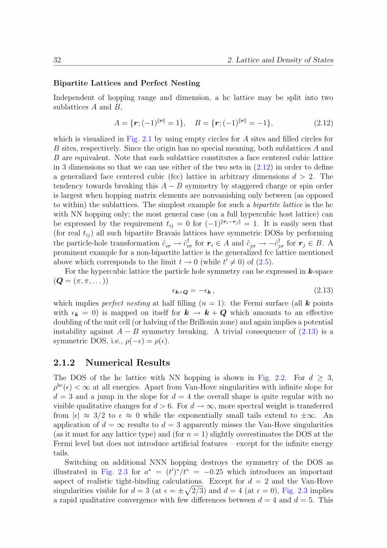
32 2. Lattice and Density of States
Bipartite Lattices and Perfect Nesting
Independent of hopping range and dimension, a hc lattice may be split into twosublattices A and B,
A = r; (−1)||r|| = 1, B = r; (−1)||r|| = −1, (2.12)
which is visualized in Fig. 2.1 by using empty circles for A sites and filled circles forB sites, respectively. Since the origin has no special meaning, both sublattices A andB are equivalent. Note that each sublattice constitutes a face centered cubic latticein 3 dimensions so that we can use either of the two sets in (2.12) in order to definea generalized face centered cubic (fcc) lattice in arbitrary dimensions d > 2. Thetendency towards breaking this A − B symmetry by staggered charge or spin orderis largest when hopping matrix elements are nonvanishing only between (as opposedto within) the sublattices. The simplest example for such a bipartite lattice is the hcwith NN hopping only; the most general case (on a full hypercubic host lattice) canbe expressed by the requirement tij = 0 for (−1)||ri−rj || = 1. It is easily seen that(for real tij) all such bipartite Bravais lattices have symmetric DOSs by performing
the particle-hole transformation ciσ → c†iσ for ri ∈ A and cjσ → −c†jσ for rj ∈ B. Aprominent example for a non-bipartite lattice is the generalized fcc lattice mentionedabove which corresponds to the limit t→ 0 (while t′ 6= 0) of (2.5).
For the hypercubic lattice the particle hole symmetry can be expressed in k-space(Q = (π, π, . . . ))
εk+Q = −εk , (2.13)
which implies perfect nesting at half filling (n = 1): the Fermi surface (all k pointswith εk = 0) is mapped on itself for k → k + Q which amounts to an effectivedoubling of the unit cell (or halving of the Brillouin zone) and again implies a potentialinstability against A − B symmetry breaking. A trivial consequence of (2.13) is asymmetric DOS, i.e., ρ(−ε) = ρ(ε).
2.1.2 Numerical Results
The DOS of the hc lattice with NN hopping is shown in Fig. 2.2. For d ≥ 3,ρhc(ε) <∞ at all energies. Apart from Van-Hove singularities with infinite slope ford = 3 and a jump in the slope for d = 4 the overall shape is quite regular with novisible qualitative changes for d > 6. For d→∞, more spectral weight is transferredfrom |ε| ≈ 3/2 to ε ≈ 0 while the exponentially small tails extend to ±∞. Anapplication of d = ∞ results to d = 3 apparently misses the Van-Hove singularities(as it must for any lattice type) and (for n = 1) slightly overestimates the DOS at theFermi level but does not introduce artificial features – except for the infinite energytails.
Switching on additional NNN hopping destroys the symmetry of the DOS asillustrated in Fig. 2.3 for a∗ = (t′)∗/t∗ = −0.25 which introduces an importantaspect of realistic tight-binding calculations. Except for d = 2 and the Van-Hovesingularities visible for d = 3 (at ε = ±
√
2/3) and d = 4 (at ε = 0), Fig. 2.3 impliesa rapid qualitative convergence with few differences between d = 4 and d = 5. This
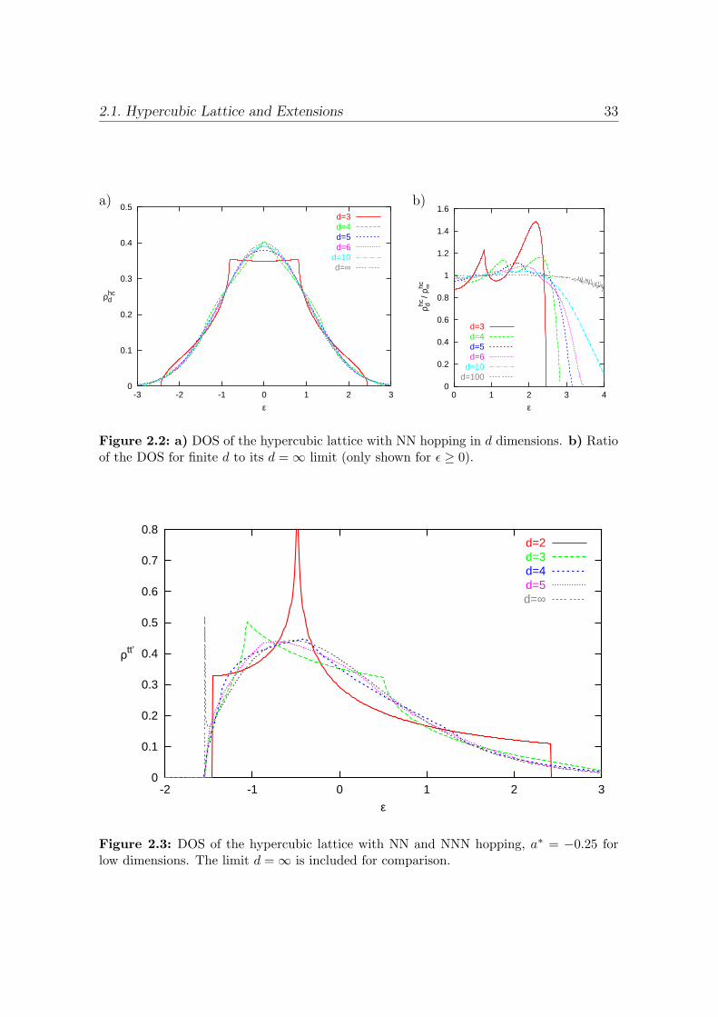
2.1. Hypercubic Lattice and Extensions 33
a) b)
0
0.1
0.2
0.3
0.4
0.5
-3 -2 -1 0 1 2 3
ρhcd
ε
d=3d=4d=5d=6
d=10d=∞
0
0.2
0.4
0.6
0.8
1
1.2
1.4
1.6
0 1 2 3 4
ρhc d /
ρhc ∞
ε
d=3d=4d=5d=6
d=10d=100
Figure 2.2: a) DOS of the hypercubic lattice with NN hopping in d dimensions. b) Ratioof the DOS for finite d to its d =∞ limit (only shown for ε ≥ 0).
0
0.1
0.2
0.3
0.4
0.5
0.6
0.7
0.8
-2 -1 0 1 2 3
ρtt’
ε
d=2d=3d=4d=5d=∞
Figure 2.3: DOS of the hypercubic lattice with NN and NNN hopping, a∗ = −0.25 forlow dimensions. The limit d =∞ is included for comparison.
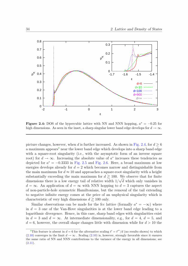
34 2. Lattice and Density of States
0
0.1
0.2
0.3
0.4
0.5
0.6
0.7
0.8
-2 -1 0 1 2 3
ρtt’
ε
d=6d=10
d=100d=900
d=∞
0
0.1
0.2
0.3
-1.7 -1.6 -1.5 -1.4
ρtt’
ε
Figure 2.4: DOS of the hypercubic lattice with NN and NNN hopping, a∗ = −0.25 forhigh dimensions. As seen in the inset, a sharp singular lower band edge develops for d→∞.
picture changes, however, when d is further increased. As shown in Fig. 2.4, for d ≥ 6a maximum appears8 near the lower band edge which develops into a sharp band edgewith a square-root singularity (i.e., with the asymptotic form of an inverse squareroot) for d → ∞. Increasing the absolute value of a∗ increases these tendencies asdepicted for a∗ = −0.3333 in Fig. 2.5 and Fig. 2.6. Here, a broad maximum at lowenergies develops already for d = 2 which becomes narrow and distinguishable fromthe main maximum for d ≈ 10 and approaches a square-root singularity with a heightsubstantially exceeding the main maximum for d & 100. We observe that for finitedimensions there is a low energy tail of relative width 1/
√d which only vanishes in
d = ∞. An application of d = ∞ with NNN hopping to d = 3 captures the aspectof non-particle-hole symmetric Hamiltonians, but the removal of the tail extendingto negative infinite energy comes at the price of an unphysical singularity which ischaracteristic of very high dimensions d & 100 only.
Similar observations can be made for the fcc lattice (formally a∗ = −∞) wherein d = 3 one of the Van-Hove singularities is at the lower band edge leading to alogarithmic divergence. Hence, in this case, sharp band edges with singularities existin d = 3 and d = ∞. At intermediate dimensionality, e.g., for d = 4, d = 5, andd = 6, however, the overall shape changes little with dimension while for d > 10 the
8This feature is absent in d = 6 for the alternative scaling t′ = t′∗/d (no results shown) to which
(2.10) converges in the limit d→∞ . Scaling (2.10) is, however, strongly favorable since it ensuresthe same ratio of NN and NNN contributions to the variance of the energy in all dimensions; see(2.11).
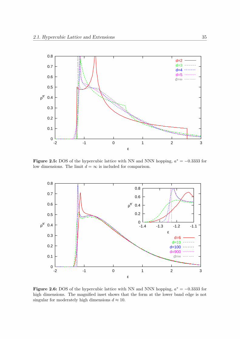
2.1. Hypercubic Lattice and Extensions 35
0
0.1
0.2
0.3
0.4
0.5
0.6
0.7
0.8
-2 -1 0 1 2 3
ρtt’
ε
d=2d=3d=4d=5d=∞
Figure 2.5: DOS of the hypercubic lattice with NN and NNN hopping, a∗ = −0.3333 forlow dimensions. The limit d =∞ is included for comparison.
0
0.1
0.2
0.3
0.4
0.5
0.6
0.7
0.8
-2 -1 0 1 2 3
ρtt’
ε
d=6d=10
d=100d=900
d=∞
0
0.2
0.4
0.6
0.8
-1.4 -1.3 -1.2 -1.1
ρtt’
ε
Figure 2.6: DOS of the hypercubic lattice with NN and NNN hopping, a∗ = −0.3333 forhigh dimensions. The magnified inset shows that the form at the lower band edge is notsingular for moderately high dimensions d ≈ 10.

36 2. Lattice and Density of States
0
0.1
0.2
0.3
0.4
0.5
0.6
0.7
0.8
0.9
1
1.1
1.2
-2 -1 0 1 2 3
ρfcc
ε
d=3d=4d=5d=6
d=10d=100
d=∞
Figure 2.7: DOS of the fcc lattice.
maximum value of ρfcc(ε) increases significantly and develops into the square-rootsingularity observed at d =∞ (see Fig. 2.7). Again, the singularity and the absenceof the lower energy tail in this limit are not robust features when the dimensionalityis decreased and thus results obtained in d = ∞ which depend on the singularity(as opposed to only a strong asymmetry) do not carry over to physically interestingdimensions.
The general behavior seen for t-t′ hopping on the hc lattice and for NN hoppingon the fcc lattice is easily explained by looking at the expressions for the energies forthe hypercube with NN hopping,
εhck = −2t
d∑
α=1
cos(kα) (2.14)
and the fcc lattice,
εfcck = 2t′d∑
α,β=1α6=β
cos(kα) cos(kβ) (2.15)
= 2t′[( d∑
α=1
cos(kα))2
−d∑
α=1
cos2(kα)]
(2.16)
= dt′[(√
2
d
d∑
α=1
cos(kα))2
− 1− 1
d
d∑
α=1
cos(2kα)]
. (2.17)
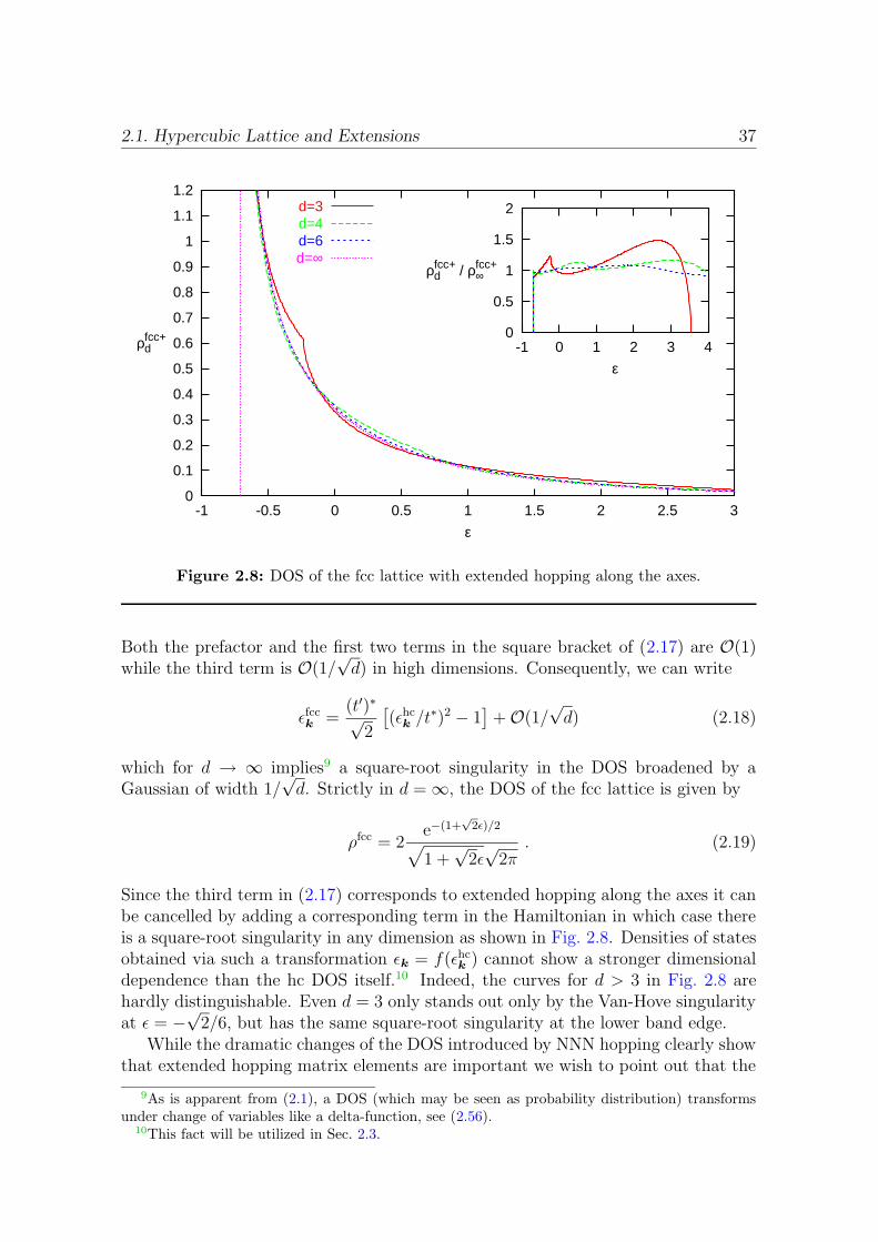
2.1. Hypercubic Lattice and Extensions 37
0
0.1
0.2
0.3
0.4
0.5
0.6
0.7
0.8
0.9
1
1.1
1.2
-1 -0.5 0 0.5 1 1.5 2 2.5 3
ρdfcc+
ε
d=3d=4d=6d=∞
0
0.5
1
1.5
2
-1 0 1 2 3 4
ρdfcc+ / ρ∞
fcc+
ε
Figure 2.8: DOS of the fcc lattice with extended hopping along the axes.
Both the prefactor and the first two terms in the square bracket of (2.17) are O(1)while the third term is O(1/
√d) in high dimensions. Consequently, we can write
εfcck =(t′)∗√
2
[(εhc
k /t∗)2 − 1
]+O(1/
√d) (2.18)
which for d → ∞ implies9 a square-root singularity in the DOS broadened by aGaussian of width 1/
√d. Strictly in d =∞, the DOS of the fcc lattice is given by
ρfcc = 2e−(1+
√2ε)/2
√
1 +√
2ε√
2π. (2.19)
Since the third term in (2.17) corresponds to extended hopping along the axes it canbe cancelled by adding a corresponding term in the Hamiltonian in which case thereis a square-root singularity in any dimension as shown in Fig. 2.8. Densities of statesobtained via such a transformation εk = f(εhc
k ) cannot show a stronger dimensionaldependence than the hc DOS itself.10 Indeed, the curves for d > 3 in Fig. 2.8 arehardly distinguishable. Even d = 3 only stands out only by the Van-Hove singularityat ε = −
√2/6, but has the same square-root singularity at the lower band edge.
While the dramatic changes of the DOS introduced by NNN hopping clearly showthat extended hopping matrix elements are important we wish to point out that the
9As is apparent from (2.1), a DOS (which may be seen as probability distribution) transformsunder change of variables like a delta-function, see (2.56).
10This fact will be utilized in Sec. 2.3.
38 2. Lattice and Density of States
inclusion of hopping elements tij with odd range D = ||ri − rj|| ≥ 3 will reintroduceinfinite-ranged low-energy tails and thus destroy the sharp band edge, one of theprominent features of t-t′ DOS in d = ∞. This issue will be treated in a broadercontext in Sec. 2.3. For the DMFT computation of transport properties for the t-t′
lattice, see subsection 4.5.3.For a discussion of the hyperdiamond lattice, see App. B.
2.1.3 Magnetic Frustration and Asymmetry of the DOS
One important question in the context of the DMFT is whether magnetic frustra-tion, in particular the suppression of antiferromagnetism, is closely related to otherproperties like the DOS and the optical conductivity or whether it can be regardedas being essentially independent, at least in high dimensions. While it is immediatelyclear that unfrustrated particle-hole symmetric systems have a symmetric DOS, theconverse statement is not generally true for Z =∞. In fact, when extended hoppingonly along the cartesic axes is introduced for the hypercubic lattice, the DOS re-mains Gaussian while for suitably chosen hopping matrix elements antiferromagneticorder is suppressed (Muller-Hartmann, 1989a). In the following, we will outline anargument why this behavior (and not only the model) should be regarded as patho-logical. First, we observe that for fixed hopping matrix elements tD to Dth-nearestneighbors along the cartesic axes the DOS in d dimensions can be obtained fromfolding the one-dimensional DOS d−1 times with itself. Since the DOS is symmetricin d = 1 if and only if the system is unfrustrated (i.e., t2n = 0 for integer n) thesame applies for all finite dimensions d. In Sec. 1.2 we have seen that perfect anticor-relation in the two-particle density of states Dq(ε1, ε2) at the antiferromagnet wavevector Q, i.e., η(Q) = −1 is associated with a strong antiferromagnetic instabilitydue to particle-hole symmetry. More generally, an instability at vector q occurs forηq ≡ η(q) ≈ −1. It seems thus reasonable to associate magnetic frustration withthe deviation of the minimum of η from −1. For the lattice under consideration it isclear that all extrema are on the diagonal q; q = λQ; 0 ≤ λ ≤ 1. For this line, wehave11 (Muller-Hartmann, 1989a)
η(λQ) =1
t2
∞∑
D=1
t2D cos(Dλπ) , (2.20)
where t2 =∑∞
D=1 t2D. First, we note that η(λQ) ≥ −1 and that η(Q) = −1 only in
the unfrustrated case where t2n = 0 for all n. For a fully quantitative analysis, werestrict hopping to NN and to NNN (along the cartesic axes). Then, the minimumof η(λQ) is for unit variance (t∗1
2 + t∗22 = 1)
ηmin =
−1 + 2t∗22 for t∗2
2 ≤ 0.2
−9t∗24−2t∗2
2+1
8t∗22 for 0.2 < t∗2
2 ≤ 1. (2.21)
11Note that (in this special case) we can use either scaled or unscaled hopping matrix elementssince the scaling factor is independent of the hopping range.

2.2. Bethe Lattice, RPE, and Disorder 39
-1
-0.5
0
0.5
1
0 0.2 0.4 0.6 0.8 1
η(λ
Q)
λ
t2*2=0.00
t2*2=0.20
t2*2=0.33
t2*2=0.50
t2*2=1.00
-1
-0.5
0
0.5
1
0 0.2 0.4 0.6 0.8 1
t2*2
<ε3>(2d)1/2
ηmin
Figure 2.9: DMFT momentum parameter η(λQ) [(1.23) and (2.20)] for the hypercubiclattice with hopping to NN and to NNN along the cartesic axes using scaled amplitudes1 − t∗22 and t∗2
2, respectively. The symmetric graph for t∗22 = 1 is not fully shown. Inset:
minimal value of η(q) and rescaled third moment of the DOS as a function of t∗22; both
frustration and asymmetry of the DOS are maximal at t∗22 = 1/3.
This value, i.e., the frustration is maximal for t∗22 = 1/3 (when η(q) ≥ −1/2 for all
q). This is exactly the value for which also the asymmetry of the DOS, measuredby its third moment, 〈ε3〉 = 6d t21t2 = 3(1− t∗22)t∗2/
√2d acquires its maximum. Thus,
for finite dimensions, maximal frustration coincides with maximal asymmetry of theDOS. This effect becomes only unobservable for Z →∞ since the associated weightbecomes exponentially small.12 The main part of Fig. 2.9 shows η(λQ) for differentvalues of t∗2
2. The minimum is at λ = 1 for t∗22 ≤ 0.2 and approaches λ = 0.5 for
t∗22 → 1 (which is again unfrustrated). The value of the minimum as a function of
t∗22 is shown in the inset together with the scaled third moment which illustrates that
maximal frustration coincides with maximal asymmetry for t∗22 = 1/3. We will find
more indications that magnetic frustration is generically associated with an asym-metry of the DOS by using the renormalized perturbation expansion in subsection2.2.2.
2.2 Bethe Lattice, RPE, and Disorder
Within this work and the DMFT literature in general, the term “Bethe lattice” ismost often used in the sense of a lattice having the “Bethe DOS”, i.e., a semi-ellipticDOS, without paying too much attention to the particular properties of this pseudo-
12Note that the ratio of the band edges, i.e., of the maximum and minimum energies, is indepen-dent of d. With respect to this criterion, the asymmetry is maximal for t∗2
2 = 1/5, where the ratiois 0.5 or 2 (depending on the signs of t1 and t2).
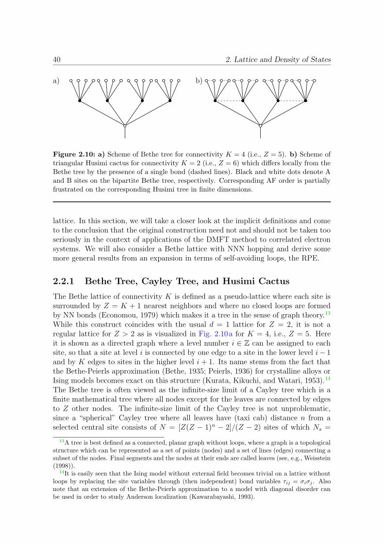
40 2. Lattice and Density of States
a) b)
Figure 2.10: a) Scheme of Bethe tree for connectivity K = 4 (i.e., Z = 5). b) Scheme oftriangular Husimi cactus for connectivity K = 2 (i.e., Z = 6) which differs locally from theBethe tree by the presence of a single bond (dashed lines). Black and white dots denote Aand B sites on the bipartite Bethe tree, respectively. Corresponding AF order is partiallyfrustrated on the corresponding Husimi tree in finite dimensions.
lattice. In this section, we will take a closer look at the implicit definitions and cometo the conclusion that the original construction need not and should not be taken tooseriously in the context of applications of the DMFT method to correlated electronsystems. We will also consider a Bethe lattice with NNN hopping and derive somemore general results from an expansion in terms of self-avoiding loops, the RPE.
2.2.1 Bethe Tree, Cayley Tree, and Husimi Cactus
The Bethe lattice of connectivity K is defined as a pseudo-lattice where each site issurrounded by Z = K + 1 nearest neighbors and where no closed loops are formedby NN bonds (Economou, 1979) which makes it a tree in the sense of graph theory.13
While this construct coincides with the usual d = 1 lattice for Z = 2, it is not aregular lattice for Z > 2 as is visualized in Fig. 2.10a for K = 4, i.e., Z = 5. Hereit is shown as a directed graph where a level number i ∈ Z can be assigned to eachsite, so that a site at level i is connected by one edge to a site in the lower level i− 1and by K edges to sites in the higher level i + 1. Its name stems from the fact thatthe Bethe-Peierls approximation (Bethe, 1935; Peierls, 1936) for crystalline alloys orIsing models becomes exact on this structure (Kurata, Kikuchi, and Watari, 1953).14
The Bethe tree is often viewed as the infinite-size limit of a Cayley tree which is afinite mathematical tree where all nodes except for the leaves are connected by edgesto Z other nodes. The infinite-size limit of the Cayley tree is not unproblematic,since a “spherical” Cayley tree where all leaves have (taxi cab) distance n from aselected central site consists of N = [Z(Z − 1)n − 2]/(Z − 2) sites of which Ns =
13A tree is best defined as a connected, planar graph without loops, where a graph is a topologicalstructure which can be represented as a set of points (nodes) and a set of lines (edges) connecting asubset of the nodes. Final segments and the nodes at their ends are called leaves (see, e.g., Weisstein(1998)).
14It is easily seen that the Ising model without external field becomes trivial on a lattice withoutloops by replacing the site variables through (then independent) bond variables τij = σiσj . Alsonote that an extension of the Bethe-Peierls approximation to a model with diagonal disorder canbe used in order to study Anderson localization (Kawarabayashi, 1993).

2.2. Bethe Lattice, RPE, and Disorder 41
Figure 2.11: Scheme of spherical Cayley tree with connectivity 2 and radius 5 (black solidlines). A selected set of NNN bonds is marked by dashed and dotted lines. Each sublatticeformed by the NNN bonds is fully frustrated with respect to AF order.
Z(Z − 1)n−1 constitute the surface (i.e., are leaves). This is illustrated in Fig. 2.11schematically for radius n = 5 and Z = 3. In the limit of infinite radius n, a finitefraction Ns/N ≈ (Z − 2)/(Z − 1) of sites is on the surface (Thorpe, 1981). A tight-binding model defined on such a Cayley tree would be dominated by surface states,in particular in the limit Z → ∞, where Ns/N → 1. This problem can be avoidedby using the bulk definition given at the beginning of the paragraph. The Bethelattice is bipartite; therefore, the generic low-temperature phase of a Hubbard modeldefined on the Bethe lattice is antiferromagnetic at half filling.
The Husimi cactus is a generalization of the Bethe lattice where each bond ispart of exactly one loop and is shown in its triangular form15 in Fig. 2.10b. For finiteZ, these loops introduce some degree of frustration. Since a single loop becomesirrelevant for Z →∞, however, all properties of the Husimi cactus converge to thatof the Bethe tree in this limit. In contrast, the inclusion of hopping along all NNNbonds (dashed lines in Fig. 2.11) leads to strong magnetic frustration in all dimensionsand to an asymmetric DOS (see subsection 2.2.2).
The absence of loops greatly simplifies not only calculations for spin models, butalso allows for an exact computation of the Green function for the noninteractingtight-binding model with nearest-neighbor hopping for arbitrary Z. Using a mean-field approach in the spirit of the Bethe-Peierls approximation (Thorpe, 1981) or therenormalized perturbation expansion around the atomic limit (Economou, 1979), one
15In the general definition of the Husimi cactus, both the type of polygons, i.e., the length ofloops, and the connectivity for each site can be chosen arbitrarily.
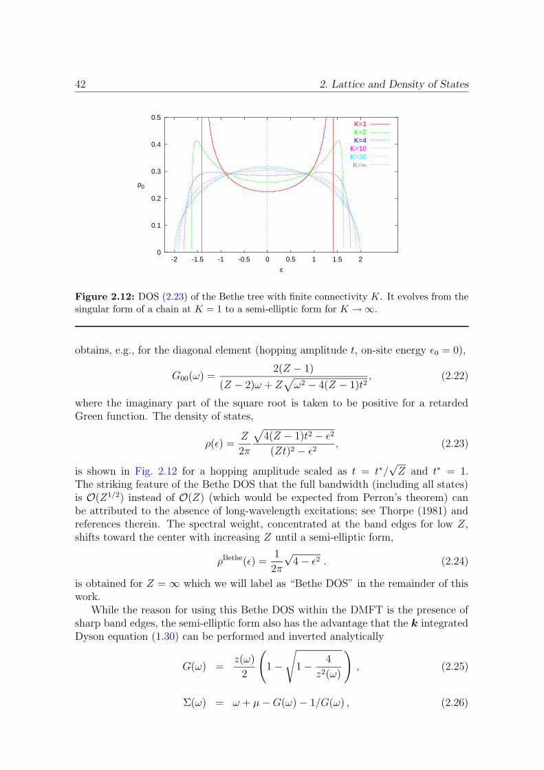
42 2. Lattice and Density of States
0
0.1
0.2
0.3
0.4
0.5
-2 -1.5 -1 -0.5 0 0.5 1 1.5 2
ρ0
ε
K=1K=2K=4
K=10K=30K=∞
Figure 2.12: DOS (2.23) of the Bethe tree with finite connectivity K. It evolves from thesingular form of a chain at K = 1 to a semi-elliptic form for K →∞.
obtains, e.g., for the diagonal element (hopping amplitude t, on-site energy ε0 = 0),
G00(ω) =2(Z − 1)
(Z − 2)ω + Z√
ω2 − 4(Z − 1)t2, (2.22)
where the imaginary part of the square root is taken to be positive for a retardedGreen function. The density of states,
ρ(ε) =Z
2π
√
4(Z − 1)t2 − ε2(Zt)2 − ε2 , (2.23)
is shown in Fig. 2.12 for a hopping amplitude scaled as t = t∗/√Z and t∗ = 1.
The striking feature of the Bethe DOS that the full bandwidth (including all states)is O(Z1/2) instead of O(Z) (which would be expected from Perron’s theorem) canbe attributed to the absence of long-wavelength excitations; see Thorpe (1981) andreferences therein. The spectral weight, concentrated at the band edges for low Z,shifts toward the center with increasing Z until a semi-elliptic form,
ρBethe(ε) =1
2π
√4− ε2 . (2.24)
is obtained for Z =∞ which we will label as “Bethe DOS” in the remainder of thiswork.
While the reason for using this Bethe DOS within the DMFT is the presence ofsharp band edges, the semi-elliptic form also has the advantage that the k integratedDyson equation (1.30) can be performed and inverted analytically
G(ω) =z(ω)
2
(
1−√
1− 4
z2(ω)
)
, (2.25)
Σ(ω) = ω + µ−G(ω)− 1/G(ω) , (2.26)
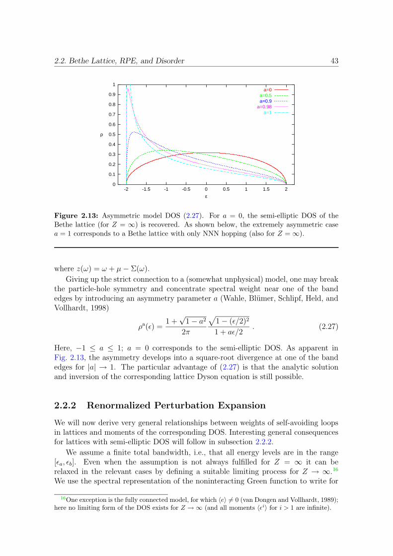
2.2. Bethe Lattice, RPE, and Disorder 43
0
0.1
0.2
0.3
0.4
0.5
0.6
0.7
0.8
0.9
1
-2 -1.5 -1 -0.5 0 0.5 1 1.5 2
ρ
ε
a=0a=0.5a=0.9
a=0.98a=1
Figure 2.13: Asymmetric model DOS (2.27). For a = 0, the semi-elliptic DOS of theBethe lattice (for Z = ∞) is recovered. As shown below, the extremely asymmetric casea = 1 corresponds to a Bethe lattice with only NNN hopping (also for Z =∞).
where z(ω) = ω + µ− Σ(ω).
Giving up the strict connection to a (somewhat unphysical) model, one may breakthe particle-hole symmetry and concentrate spectral weight near one of the bandedges by introducing an asymmetry parameter a (Wahle, Blumer, Schlipf, Held, andVollhardt, 1998)
ρa(ε) =1 +√
1− a2
2π
√
1− (ε/2)2
1 + aε/2. (2.27)
Here, −1 ≤ a ≤ 1; a = 0 corresponds to the semi-elliptic DOS. As apparent inFig. 2.13, the asymmetry develops into a square-root divergence at one of the bandedges for |a| → 1. The particular advantage of (2.27) is that the analytic solutionand inversion of the corresponding lattice Dyson equation is still possible.
2.2.2 Renormalized Perturbation Expansion
We will now derive very general relationships between weights of self-avoiding loopsin lattices and moments of the corresponding DOS. Interesting general consequencesfor lattices with semi-elliptic DOS will follow in subsection 2.2.2.
We assume a finite total bandwidth, i.e., that all energy levels are in the range[εa, εb]. Even when the assumption is not always fulfilled for Z = ∞ it can berelaxed in the relevant cases by defining a suitable limiting process for Z → ∞.16
We use the spectral representation of the noninteracting Green function to write for
16One exception is the fully connected model, for which 〈e〉 6= 0 (van Dongen and Vollhardt, 1989);here no limiting form of the DOS exists for Z →∞ (and all moments 〈εi〉 for i > 1 are infinite).

44 2. Lattice and Density of States
ω > max|εa|, |εb|
G(ω) =
εb∫
−εa
dερ(ε)
ω − ε =
εb∫
−εa
dε ρ(ε)1
ω
∞∑
i=0
( ε
ω
)i
=∞∑
i=0
〈εi〉ωi+1
. (2.28)
Thus, the high-frequency behavior of G is easily obtained from moments of the DOSand vice versa. Obviously, a necessary condition for (2.28) and the following conclu-sions to hold is that all moments 〈εi〉 exist.
The Renormalized Perturbation Expansion (RPE) is an expansion in the hoppingmatrix elements around the atomic limit where all contributions to the local Greenfunction for some site i can be obtained by considering all decorated self-avoidingloops starting and ending at i. While in finite dimensions the decorations must becomputed in terms of special self-avoiding loops which do not touch any site alreadycontained in loops of lower hierarchy, this restriction becomes irrelevant in the limitZ → ∞ where the decorations are nothing but full local Green functions. Thus,for the simplest case of full translational symmetry one arrives at a single closedself-consistency equation for some site i,
G−1(ω) = ω −(
G∑
j
t2ij +G2∑
j 6=ktijtjktki +G3
∑
j 6=k 6=l;j 6=ltijtjktkltli + . . .
)
(2.29)
=: ω −∞∑
n=2
anGn−1 , (2.30)
where the coefficients an measure the weight of self-avoiding loops of length n. Notethat when all nonzero hopping matrix elements are equal, the simpler expression an =tnNn applies, where Nn is the number of self-avoiding loops of length n originatingfrom site i which implies a one-to-one correspondence between the DOS and thetopology of the lattice.
Multiplying (2.30) by G and inserting the expansion (2.28) we can compute mo-ments of the DOS from the hopping weights order by order
〈ε0〉 = 1 ; 〈ε1〉 = 0 ; 〈ε2〉 = a2 . (2.31)
Enforcing, for simplicity, unit variance by setting the weight a2 of 2-loops to 1, thehigher order moments read
〈ε2〉 = 1 ; 〈ε3〉 = a3 (2.32)
〈ε4〉 = 2 + a4 ; 〈ε5〉 = 2 + 3a3 + a5 . (2.33)
It is easy to check that only (2.33) and corresponding higher order expressions arespecific to d =∞, while (2.32) also applies to finite dimensions: the third moment ofany DOS is directly determined only by the weight of self-avoiding 3-loops (i.e., thescaled number of 3-loops if all nonvanishing matrix elements are equal for a trans-lation invariant lattice, 〈ε3〉 = t3N3). We can thus spot one of the most prominent
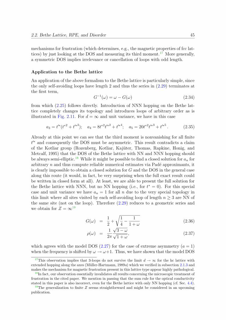
2.2. Bethe Lattice, RPE, and Disorder 45
mechanisms for frustration (which determines, e.g., the magnetic properties of fcc lat-tices) by just looking at the DOS and measuring its third moment.17 More generally,a symmetric DOS implies irrelevance or cancellation of loops with odd length.
Application to the Bethe lattice
An application of the above formalism to the Bethe lattice is particularly simple, sincethe only self-avoiding loops have length 2 and thus the series in (2.29) terminates atthe first term,
G−1(ω) = ω −G(ω) (2.34)
from which (2.25) follows directly. Introduction of NNN hopping on the Bethe lat-tice completely changes its topology and introduces loops of arbitrary order as isillustrated in Fig. 2.11. For d =∞ and unit variance, we have in this case
a3 = t′∗(t∗2 + t′∗2); a4 = 8t∗2t′∗
2+ t′∗
4; a5 = 20t∗2t′∗
3+ t′∗
5. (2.35)
Already at this point we can see that the third moment is nonvanishing for all finitet′∗ and consequently the DOS must be asymmetric. This result contradicts a claimof the Kotliar group (Rozenberg, Kotliar, Kajuter, Thomas, Rapkine, Honig, andMetcalf, 1995) that the DOS of the Bethe lattice with NN and NNN hopping shouldbe always semi-elliptic.18 While it might be possible to find a closed solution for an forarbitrary n and thus compute reliable numerical estimates via Pade approximants, itis clearly impossible to obtain a closed solution for G and the DOS in the general casealong this route (it would, in fact, be very surprising when the full exact result couldbe written in closed form at all). At least, we are able to present the full solution forthe Bethe lattice with NNN, but no NN hopping (i.e., for t∗ = 0). For this specialcase and unit variance we have an = 1 for all n due to the very special topology inthis limit where all sites visited by each self-avoiding loop of length n ≥ 3 are NN ofthe same site (not on the loop). Therefore (2.29) reduces to a geometric series andwe obtain for Z =∞19
G(ω) =1
2+
√
1
4− 1
1 + ω(2.36)
ρ(ω) =1
2π
√3− ω√1 + ω
, (2.37)
which agrees with the model DOS (2.27) for the case of extreme asymmetry (a = 1)when the frequency is shifted by ω → ω+1. Thus, we have shown that the model DOS
17This observation implies that 3-loops do not survive the limit d → ∞ for the hc lattice withextended hopping along the axes (Muller-Hartmann, 1989a) which we verified in subsection 2.1.3 andmakes the mechanism for magnetic frustration present in this lattice type appear highly pathological.
18In fact, our observation essentially invalidates all results concerning the microscopic treatment offrustration in the cited paper. We mention in passing that the sum rule for the optical conductivitystated in this paper is also incorrect, even for the Bethe lattice with only NN hopping (cf. Sec. 4.4).
19The generalization to finite Z seems straightforward and might be considered in an upcomingpublication.
46 2. Lattice and Density of States
interpolates between Bethe lattices for Z =∞ with only NN and only NNN hopping.In order to exclude that there is an accidental connection to the microscopic modelalso for 0 < a < 1, we determined the leading nontrivial corresponding moments ofthe DOS (2.27) for a = 0.9 (which are 〈(ε − 〈ε〉)3〉 ≈ 0.6268, 〈(ε − 〈ε〉)4〉 ≈ 2.3929,〈(ε − 〈ε〉)5〉 ≈ 3.3802) and fixed the ratio t′∗/t∗ ≈ 0.2208 to fulfill (2.32) and (2.35).This leads to a4 = 0.3568, a5 = 0.1917 and corresponds to 4th and 5th moments of2.3568 and 4.0720, respectively. Clearly, the results are not compatible; a5 wouldeven have to have the opposite sign in order to reproduce the 5th moment of themodel DOS.
From the above we may further conclude that the weights an for self-avoidingloops of length n > 2 must cancel exactly also for the tight-binding Hamiltonianhaving a semi-elliptic DOS which we will construct in the following section. Whilethis consideration implies that the Bethe tree is the only (pseudo)lattice with semi-elliptic DOS and only one nonzero hopping parameter it could in principle also beused to verify or even construct Hamiltonians. In practice, however, there exist manycontributions, e.g., to the sum over 4-loops on hypercubic lattices, even for a small setof longer range hopping terms. For hopping t to NN and t3 to 3rd-nearest neighborswe found on the hc lattice the leading contribution
a4 ≈ t∗4 + 36t∗2t∗32 + 4
√6t∗3t∗3 + 48
√6t∗t∗3
3 + 108t∗34 (2.38)
which adds up to -0.04 when the values from Table 2.1 (page 55) are used. Con-tributions from longer-range hopping are larger than might be expected from thesmall value of this partial sum. One contribution is, e.g., 12
√20t∗2t∗3t
∗5 ≈ −0.31. We
find it remarkable that the semi-elliptic DOS imposes such severe constraints (i.e.,the cancellation of all loops of length greater than 2) on corresponding tight-bindingmodels, even though this criterion appears not to be of general constructive value.
Off-diagonal disorder
One further application where the RPE can provide much insight is off-diagonaldisorder. For independent random variables tij, all contributions from self-avoidingloops of order n > 2 vanish exactly as long as the hopping elements vanish on average,〈tij〉 = 0. The remarkable conclusion is that noninteracting Green function and DOSagree with that of the Bethe lattice (with NN hopping) for arbitrary topology in thiscase. This statement, valid for Z = ∞, is more general than Wegner’s treatment of“gauge invariant” tight-binding models which predicts local Bethe lattice propertiesonly for systems with a fully symmetric distribution of hopping matrix elements,〈t2n+1ij 〉 = 0 (Wegner, 1976). In our view, the tighter restrictions for finite Z can be
linked to the fact that in this case not only the weight of self-avoiding loops, but ofall loops (of length n > 2) has to vanish in order to reduce the effective mean freepath to one lattice spacing, which is the physics of all models with Bethe DOS. Inthe context of DMFT calculations, frustration caused by disorder of the above typewas considered for a fully connected model (Georges and Krauth, 1993) and thenalso for the more general cases (Dobrosavljevic and Kotliar, 1993; Dobrosavljevicand Kotliar, 1994).
2.3. General Density of States in d =∞ 47
As a last conclusion from this section let us note that additional hopping (e.g.,along NNN bonds) does not modify the semi-elliptic DOS of the Bethe lattice whenthese additional bonds are fully disordered (with zero mean hopping amplitudes). Incontrast to the clean case it is, thus, possible to tune magnetic frustration in such asystem by variation of 〈t∗22〉 at constant DOS.20
2.3 General Density of States in d = ∞
In this section, we will present a general algorithm for finding an isotropic, transla-tionally invariant tight-binding Hamiltonian corresponding to an arbitrary DOS ind = ∞. While the availability of such a method to construct a microscopic Hamil-tonian corresponding to some model DOS might be useful in any dimension, it isabsolutely essential for considering spatially inhomogeneous phases (e.g, antiferro-magnetism or charge density waves) or computing transport properties within theDMFT. The algorithm developed in this section will later enable us to perform thefirst fully consistent DMFT calculation of the optical conductivity for a periodic andisotropic lattice (cf. footnote 3 on page 28) with the Bethe semi-elliptic DOS (seeSec. 4.4).
Scaling Relations
We start by rewriting the usual noninteracting Hamiltonian with general (transla-tionally invariant) hopping,21
H0 =∑
ij,σ
tij c†Riσ
cRjσ=∑
i,σ
∑
τ
tτ c†Riσ
cRi+τ ,σ (2.39)
=∑
k,σ
ε(k)nkσ, (2.40)
where
ε(k) =∑
τ
tτeiτ ·k =∑
τ
(tτ + t∗τ2
cos(τ · k) + itτ − t∗τ
2sin(τ · k)
)
. (2.41)
Classifying the hopping vectors τ according to their length measured by the taxi-cabmetric, we may split up the kinetic energy accordingly,
ε(k) =∞∑
D=1
εD(k), εD(k) =∑
||τ ||=Dtτeiτ ·k . (2.42)
For D > 1, each set of vectors τ ; ||τ || = D consists of different subsets whichare pairwise inequivalent such as, for D = 2, the subsets τ ; τ = ±eα ± eβ;α 6=
20The same applies to the regular, translation invariant model with semi-elliptic DOS which wewill construct in the next section: additional even-range disorder hopping terms could introducefrustration without changing the DOS.
21For sake of clarity, we write ε(k) instead of εk for the full dispersion [i.e., the full sum in (2.42)]throughout this section.
48 2. Lattice and Density of States
β and τ ; τ = ±2eα. Consequently, one may expect the corresponding hoppingamplitudes to be different. We will choose to neglect all hopping vectors with |τ ·eα| >1 for any direction α, i.e., only consider vectors of the form τ =
∑Di=1 eαi
with pairwisedifferent directions αi. This selection can be justified by the following observations:
• For fixed ||τ ||, the vectors considered are of minimal Euclidean length |τ | hintingat maximal overlap, i.e., largest |tτ |.
• The fraction of neglected vectors is O(1/d) in high dimensions (as long asdÀ D, cf. footnote 5 on page 30).
For real (and therefore symmetric) hopping amplitudes22 and in the isotropic case,the amplitudes tτ are functions of D = ||τ || alone, εD(k) = tD
∑
||τ ||=D eiτ ·k. As in
the case of t-t′ hopping (which corresponds to D = 1, 2 in the present scheme), thereare no cross terms in the variance
〈ε2(k)〉 =∑
τ ,τ′
tτtτ ′〈ei(τ−τ′)·k〉 =∑
τ
|tτ |2 =∑
D
〈ε2D(k)〉 (2.43)
〈ε2D(k)〉 = t2DND; ND = 2D(d
D
)
≈ (2d)D
D!. (2.44)
Here, ND is the number of hopping terms in shell D and the approximation in (2.44)is valid for d À D. In order for the total variance to remain finite, the amplitudestD must be scaled as tD = t∗D/
√ND, which is consistent with (2.10) and leads to
〈ε2(k)〉 =∞∑
D=1
〈ε2D(k)〉 =∞∑
D=1
t∗D2 . (2.45)
Hopping Matrix Elements and Dispersion; Transformation Function F(ε)
Now we have
εD(k) = tD2D∑
αD>αD−1>···>α1
cos(kαD) cos(kαD−1
) . . . cos(kα1) (2.46)
= tD2D
D!
(d
2
)D/2
BD(k), (2.47)
where the functions
BD(k) =
(2
d
)D/2 ∑
αD 6=αD−1 6=···6=α1
cos(kαD) cos(kαD−1
) . . . cos(kα1) (2.48)
22Note that while Eqn. (1.10) always yields real tij for atomic orbitals, this is not generally true forWannier orbitals where phase factors may arise. In a single-band description, however, a restrictionto the s-band case of real and isotropic hopping amplitudes is natural since the full Hamiltonianshould have the symmetry of the lattice.
2.3. General Density of States in d =∞ 49
fulfill a recursion relation in d =∞,
BD+1(k) = B1(k)BD(k)−DBD−1(k)2
d
d∑
α=1
cos2(kα) +O(1/d)
= B1(k)BD(k)−DBD−1(k) +O(1/√d) . (2.49)
To leading order, this relation is very similar to that of the Hermite polynomials23
Hen+1(x) = xHen(x)− nHen−1(x) . (2.50)
From (2.49), (2.50), and B0 = 1 we conclude that BD(k) = HeD(B1(k)). Further-more, we can express the argument x in (2.50) as the dispersion of the hypercubiclattice with a positive hopping term [i.e., t∗ = −1 in (1.14)] and unit variance:B1(k) = εhc
k . Consequently, we obtain
εD(k) = tD2D
D!
(d
2
)D/2
HeD(B1(k)) (2.51)
and
ε(k) =∞∑
D=1
t∗D√D!
HeD(εhck ) =: F(εhc
k ) . (2.52)
Finding not only an effectively one-dimensional expression, but even a closed form(2.52) for the general dispersion of a hypercubic lattice with arbitrary-range hoppingin terms of scaled hopping matrix elements is clearly a significant result. On the onehand, this expression applies to all such models where the hopping amplitudes de-pend on taxi-cab distance and therefore systematically classifies most models studiedin the DMFT literature. On the other hand, (2.52) will enable us to explore in-formation hidden in any given DOS, namely the dispersion and the scaled hoppingmatrix elements of a corresponding model (in d =∞), as we will show in the follow-ing. Since any analytic function can be expanded in Hermite polynomials using theorthogonality relation
∞∫
−∞
dxHen(x) Hem(x)e−x
2/2
√2π
= n! δmn, (2.53)
we can find hopping amplitudes t∗D so that ε(k) = F(εhck ) for an arbitrary analytic
function F . As an illustration of this expansion, we rescale the Hermite polynomialsin Fig. 2.14a to
pD(x) := HeD(x)/√D! . (2.54)
The full transformation function is then a linear combination of the basis functionspD where the Euclidean norm of the vector of expansion coefficients t∗D sets the energyscale for the resulting DOS.
23For the two different definitions of the Hermite polynomials with Hn(x) = 2n/2Hen(√
2x) see,e.g., Abramowitz and Stegun (1972).
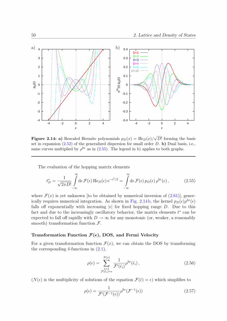
50 2. Lattice and Density of States
a) b)
-4
-3
-2
-1
0
1
2
3
4
-4 -2 0 2 4
p D(ε
)
ε
-0.4
-0.3
-0.2
-0.1
0
0.1
0.2
0.3
0.4
-4 -2 0 2 4
ρhc(ε
) p D
(ε)
ε
D=1D=2D=3D=4D=5
D=10
Figure 2.14: a) Rescaled Hermite polynomials pD(x) = HeD(x)/√D! forming the basis
set in expansion (2.52) of the generalized dispersion for small order D. b) Dual basis, i.e.,same curves multiplied by ρhc as in (2.55). The legend in b) applies to both graphs.
The evaluation of the hopping matrix elements
t∗D =1√
2πD!
∞∫
−∞
dεF(ε) HeD(ε) e−ε2/2 =
∞∫
−∞
dεF(ε) pD(ε) ρhc(ε) , (2.55)
where F(x) is yet unknown [to be obtained by numerical inversion of (2.61)], gener-ically requires numerical integration. As shown in Fig. 2.14b, the kernel pD(ε)ρhc(ε)falls off exponentially with increasing |ε| for fixed hopping range D. Due to thisfact and due to the increasingly oscillatory behavior, the matrix elements t∗ can beexpected to fall off rapidly with D →∞ for any monotonic (or, weaker, a reasonablysmooth) transformation function F .
Transformation Function F(ε), DOS, and Fermi Velocity
For a given transformation function F(x), we can obtain the DOS by transformingthe corresponding δ-functions in (2.1),
ρ(ε) =
N(ε)∑
i=1F(εi)=ε
1
F ′(εi)ρhc(εi) , (2.56)
(N(ε) is the multiplicity of solutions of the equation F(ε) = ε) which simplifies to
ρ(ε) =1
F ′(F−1(ε))ρhc(F−1(ε)) (2.57)
2.3. General Density of States in d =∞ 51
for a monotonic (i.e., invertible) function24 F(x). In order to solve for F(x) we formthe integral
ε∫
−∞
dε′ρ(ε′) =
ε∫
−∞
dε ′ρhc(ε ′); ε = F(ε) , (2.58)
which leads to
R(F(ε)) = erf(ε/√
2), R(ε) := 2
ε∫
−∞
dε′ρ(ε′)− 1 . (2.59)
We obtain
F(ε) = R−1(erf(ε/√
2)) ⇔ F−1(ε) =√
2 erf−1(R(ε)) (2.60)
or, summarizing,
F−1(ε) =√
2 erf−1
(
2
ε∫
−∞
dε′ρ(ε′)− 1
)
. (2.61)
This concludes our presentation of the general algorithm for constructing a tight-binding Hamiltonian, i.e., hopping matrix elements, from a given DOS in d = ∞based on ideas developed by van Dongen (2001).
For later use we also evaluate the Fermi velocity, vk. From (2.57) and (2.60) wehave
F ′(F−1(ε)) =ρhc(√
2 erf−1(R(ε)))
ρ(ε)(2.62)
which we can use for computing
vk = ∇F(εhck ) = F ′(F−1(ε))vhc
k (2.63)
by numerical integration and application of the inverse error function. As will bediscussed in detail in subsection 2.4.1 and chapter 4, the behavior of the squaredFermi velocity 〈|vk|2〉(ε) := ρ(ε)/ρ(ε) [cf. definitions (2.1) and (2.2)] dramaticallychanges from that observed in the hc lattice: for any nontrivial transformation itis no longer effectively constant but depends strongly on energy. In particular, theFermi velocity vanishes at the band edges as physically required in any dimension.
A practical application of the general dispersion formalism proceeds as followsfrom a given target DOS ρ(ε):
1. compute F−1(ε) using (2.61)
2. invert numerically or analytically to obtain F(ε)
3. evaluate transport properties, e.g., 〈|vk|2〉(ε) or ρ(ε) using (2.62) and (2.63)
24Here and in the following, F−1 denotes the functional inverse, not the fraction 1/F .
52 2. Lattice and Density of States
4. optionally: determine microscopic model parameters, i.e., the hopping matrixelements t∗D using (2.55)
The only choice inherent in this procedure beyond the usual assumptions for largedimensions is contained in step 1 which by construction produces a monotonic trans-formation function F .
Example: Flat-band System
One interesting limiting case of a monotonic transformation function which we cantreat analytically is the step function F(x) = 2Θ(x)− 1 corresponding to a flat bandDOS, ρ(ε) = (δ(ε− 1) + δ(ε+ 1))/2. Due to the nonanalytic step at ε = 0 we expectthe decay of the hopping matrix elements t∗D to be much slower than in generic cases,at least for monotonic F . Using the identity
x∫
0
dy e−y2/2Hen(y) = Hen−1(0)− e−x
2/2Hen−1(x) (2.64)
for x = ∞ and He2n(0) = (−1)n(2n− 1)!!, He2n+1(0) = 0 we can evaluate (2.55) forthe case at hand (trivially, t∗2n = 0):
t∗2n+1 =2
√
2π(2n+ 1)!
∞∫
0
dεHe2n+1(ε) e−ε2/2 (2.65)
= (−1)n√
2
π
(2n− 1)!!√
(2n+ 1)!(2.66)
n→∞−→ (−1)n(πn)−3/4 . (2.67)
The asymptotic form, obtained by applying the Stirling formula and retaining onlyleading powers of n, is accurate to within 1% for n > 30. As expected, t∗2n+1 fallsoff slowly; the power −3/4 is only slightly smaller than the threshold value −1/2required for the convergence of the sum
∑
D t∗D
2. Correspondingly, the transformationfunction converges only slowly to its limiting form. Both the hopping matrix elementsand the transformation functions, corresponding to truncated series expansions withD ≤ 2N+1, are shown in Fig. 2.15. We do not attempt to calculate truncation effectsfor the DOS for this toy model which is complicated due to the many branches formedby the oscillatory truncated transformation functions. Still, the main features of theDOS for a model with truncated hopping range are clear: the two δ-peaks (of theDmax = ∞ model) are broadened with a potentially irregular shape, while a finitedensity of states remains at ε = 0 for finite maximal hopping range. Furthermore, wecan read off from (2.67) and (2.71) that the gap develops very slowly for Dmax →∞with ρ(0) ∝ D
−1/2max .
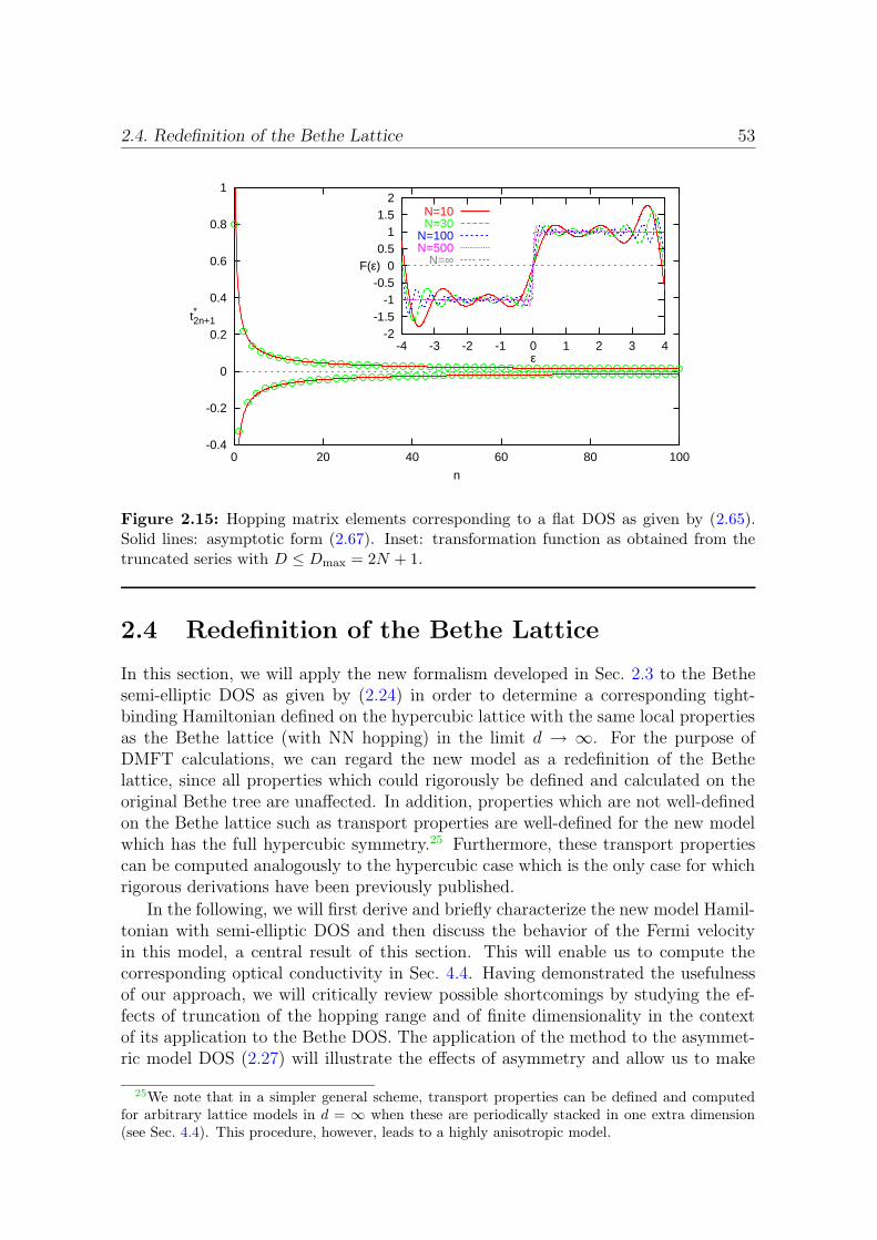
2.4. Redefinition of the Bethe Lattice 53
-0.4
-0.2
0
0.2
0.4
0.6
0.8
1
0 20 40 60 80 100
t*2n+1
n
-2-1.5
-1-0.5
00.5
11.5
2
-4 -3 -2 -1 0 1 2 3 4
F(ε)
ε
N=10N=30
N=100N=500
N=∞
Figure 2.15: Hopping matrix elements corresponding to a flat DOS as given by (2.65).Solid lines: asymptotic form (2.67). Inset: transformation function as obtained from thetruncated series with D ≤ Dmax = 2N + 1.
2.4 Redefinition of the Bethe Lattice
In this section, we will apply the new formalism developed in Sec. 2.3 to the Bethesemi-elliptic DOS as given by (2.24) in order to determine a corresponding tight-binding Hamiltonian defined on the hypercubic lattice with the same local propertiesas the Bethe lattice (with NN hopping) in the limit d → ∞. For the purpose ofDMFT calculations, we can regard the new model as a redefinition of the Bethelattice, since all properties which could rigorously be defined and calculated on theoriginal Bethe tree are unaffected. In addition, properties which are not well-definedon the Bethe lattice such as transport properties are well-defined for the new modelwhich has the full hypercubic symmetry.25 Furthermore, these transport propertiescan be computed analogously to the hypercubic case which is the only case for whichrigorous derivations have been previously published.
In the following, we will first derive and briefly characterize the new model Hamil-tonian with semi-elliptic DOS and then discuss the behavior of the Fermi velocityin this model, a central result of this section. This will enable us to compute thecorresponding optical conductivity in Sec. 4.4. Having demonstrated the usefulnessof our approach, we will critically review possible shortcomings by studying the ef-fects of truncation of the hopping range and of finite dimensionality in the contextof its application to the Bethe DOS. The application of the method to the asymmet-ric model DOS (2.27) will illustrate the effects of asymmetry and allow us to make
25We note that in a simpler general scheme, transport properties can be defined and computedfor arbitrary lattice models in d = ∞ when these are periodically stacked in one extra dimension(see Sec. 4.4). This procedure, however, leads to a highly anisotropic model.

54 2. Lattice and Density of States
contact with a related approach.
2.4.1 Model in d = ∞
A practical application of the theory outlined in Sec. 2.3 always proceeds in two steps:first, one has to find the energy transformation function F which relates the “target”DOS to the DOS of the hypercubic lattice [cf. (2.57)] and suffices for the computationof all transport related properties discussed in this work. In a second step one mayfully determine the underlying microscopic tight-binding model by computing thecorresponding scaled hopping matrix elements.
In order to determine the inverse of the transformation function via (2.60), weneed to compute the function R defined in (2.59) in terms of an integral over theDOS.26 Using (2.24) for unit variance, R can be obtained in closed form,
R(ε) = −1 +2
π
ε∫
−2
dε′√
1− ε′2/4
=1
π
(
ε√
1− ε2/4 + 2 sin−1(ε/2))
. (2.68)
Since we defined the function F to be smooth and monotonic, it can easily be ob-tained from F−1(ε) =
√2 erf−1(R(ε)) using numerical root-finding algorithms. The
transformation function shown as solid line in Fig. 2.16a is monotonic, antisymmetric,and smoothly approaches an asymptotic value of +2 (−2) for very high (low) energiesε. Keeping in mind that F was defined as a mapping function which when appliedto the hc DOS (i.e., energy levels with a Gaussian distribution function) yields thetarget DOS, we see that the boundedness of F guarantees sharp band edges, whilethe linearity at small energies with a slope greater than one flattens out the centralpart of the DOS compared to the hc case [cf. (2.71)]. Slight variations of the trans-formation functions only lead to a slight redistribution of spectral weight. This canbe illustrated by replacing the (analytically inaccessible) transformation function Fby a hyperbolic tangent,
F(ε) ≈ a tanh
(√π
2aε
)
; a ≈ 2.176, (2.69)
where the coefficients were chosen subject to the requirements that the correspondingDOS has unit variance and that it agrees with the Bethe DOS for |ε| → 0. Due tothe boundedness we again obtain sharp band edges, now with finite slopes; otherwisethe “tanh” DOS is hardly distinguishable from the semi-elliptic Bethe DOS, as seenin Fig. 2.16b.
In order to determine the microscopic model, we have to apply (2.55) to thenumerically evaluated transformation function F . As shown in Table 2.1, the scaledhopping matrix elements fall off exponentially fast – only a fraction 10−3 of the totalenergy variance arises from hopping amplitudes beyond 3rd-nearest neighbors and
26Note that R(µ) = 2n(µ)− 1 when n is the electron filling for a chemical potential µ at T = 0.

2.4. Redefinition of the Bethe Lattice 55
-2
-1.5
-1
-0.5
0
0.5
1
1.5
2
-4 -2 0 2 4
ε
~ε
Bethe"tanh"
0
0.1
0.2
0.3
0.4
0 0.5 1 1.5 2
ρ
ε
Bethe"tanh"
hc
Figure 2.16: Transformation function ε = F(ε) for the semi-elliptic Bethe DOS: numer-ically exact result and approximation by a hyperbolic tangent according to (2.69). Theinset shows corresponding DOSs [cf. (2.57)] in comparison to the Gaussian DOS of the hclattice.
D t∗D∑D
n=1 t∗n2 D t∗D
∑Dn=1 t
∗n2
1 0.98731 0.974773 9 0.00343 0.9999993 -0.15353 0.998345 11 -0.00108 1.0000005 0.03893 0.999861 13 0.00033 1.0000007 -0.01125 0.999987 15 -0.00011 1.000000
Table 2.1: Leading scaled hopping matrix elements corresponding to a semi-elliptic BetheDOS. The columns consisting of partial sums indicate rapid convergence of the series: onlya fraction 1 −∑D
n=1 t∗n2 of the variance arises from hopping terms beyond Dth neighbors.
The mean squared hopping distance is∑∞
D=1D t∗D2 ≈ 1.05406.
only a fraction 10−6 results from hopping beyond 9th-nearest neighbors. Since sucha short average range is certainly within physical limits for any itinerant system, ourmodel seems a no less natural description for systems involving narrow tight-bindingorbitals than the Hubbard model (with only NN hopping) itself. The situation wouldbe different if we had found slow algebraic decay of the hopping amplitudes like wehave seen for the toy flat band example, (2.67), which made the latter appear ratherunphysical.
Using (2.62) and (2.63), we can compute the averaged squared Fermi velocity〈|vk|2〉(ε), where for each value of ε the average is taken over all momenta k with
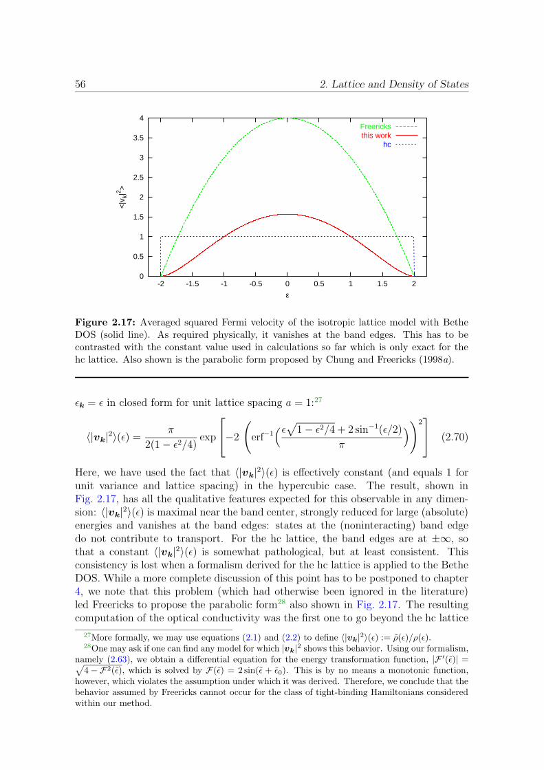
56 2. Lattice and Density of States
0
0.5
1
1.5
2
2.5
3
3.5
4
-2 -1.5 -1 -0.5 0 0.5 1 1.5 2
<|v
k|2 >
ε
Freericksthis work
hc
Figure 2.17: Averaged squared Fermi velocity of the isotropic lattice model with BetheDOS (solid line). As required physically, it vanishes at the band edges. This has to becontrasted with the constant value used in calculations so far which is only exact for thehc lattice. Also shown is the parabolic form proposed by Chung and Freericks (1998a).
εk = ε in closed form for unit lattice spacing a = 1:27
〈|vk|2〉(ε) =π
2(1− ε2/4) exp
−2
(
erf−1(ε√
1− ε2/4 + 2 sin−1(ε/2)
π
))2
(2.70)
Here, we have used the fact that 〈|vk|2〉(ε) is effectively constant (and equals 1 forunit variance and lattice spacing) in the hypercubic case. The result, shown inFig. 2.17, has all the qualitative features expected for this observable in any dimen-sion: 〈|vk|2〉(ε) is maximal near the band center, strongly reduced for large (absolute)energies and vanishes at the band edges: states at the (noninteracting) band edgedo not contribute to transport. For the hc lattice, the band edges are at ±∞, sothat a constant 〈|vk|2〉(ε) is somewhat pathological, but at least consistent. Thisconsistency is lost when a formalism derived for the hc lattice is applied to the BetheDOS. While a more complete discussion of this point has to be postponed to chapter4, we note that this problem (which had otherwise been ignored in the literature)led Freericks to propose the parabolic form28 also shown in Fig. 2.17. The resultingcomputation of the optical conductivity was the first one to go beyond the hc lattice
27More formally, we may use equations (2.1) and (2.2) to define 〈|vk|2〉(ε) := ρ(ε)/ρ(ε).28One may ask if one can find any model for which |vk|2 shows this behavior. Using our formalism,
namely (2.63), we obtain a differential equation for the energy transformation function, |F ′(ε)| =√
4−F2(ε), which is solved by F(ε) = 2 sin(ε + ε0). This is by no means a monotonic function,however, which violates the assumption under which it was derived. Therefore, we conclude that thebehavior assumed by Freericks cannot occur for the class of tight-binding Hamiltonians consideredwithin our method.
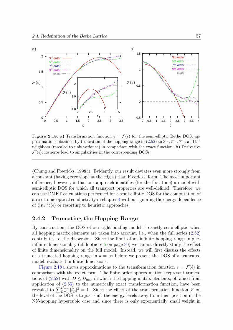
2.4. Redefinition of the Bethe Lattice 57
a) b)
F(ε) F(ε)
F(ε)
0
0.5
1
1.5
2
0 0.5 1 1.5 2 2.5 3 3.5~ε
3rd order5th order7th order9th order
exact
1.8
1.9
2
2 2.5 3 3.5~ε
-0.5
0
0.5
1
1.5
0 0.5 1 1.5 2 2.5 3 3.5 4~ε
3rd order5th order7th order9th order
exact
Figure 2.18: a) Transformation function ε = F(ε) for the semi-elliptic Bethe DOS: ap-proximations obtained by truncation of the hopping range in (2.52) to 3rd, 5th, 7th, and 9th
neighbors (rescaled to unit variance) in comparison with the exact function. b) DerivativeF ′(ε); its zeros lead to singularities in the corresponding DOSs.
(Chung and Freericks, 1998a). Evidently, our result deviates even more strongly froma constant (having zero slope at the edges) than Freericks’ form. The most importantdifference, however, is that our approach identifies (for the first time) a model withsemi-elliptic DOS for which all transport properties are well-defined. Therefore, wecan use DMFT calculations performed for a semi-elliptic DOS for the computation ofan isotropic optical conductivity in chapter 4 without ignoring the energy dependenceof 〈|vk|2〉(ε) or resorting to heuristic approaches.
2.4.2 Truncating the Hopping Range
By construction, the DOS of our tight-binding model is exactly semi-elliptic whenall hopping matrix elements are taken into account, i.e., when the full series (2.52)contributes to the dispersion. Since the limit of an infinite hopping range impliesinfinite dimensionality (cf. footnote 5 on page 30) we cannot directly study the effectof finite dimensionality on the full model. Instead, we will first discuss the effectsof a truncated hopping range in d = ∞ before we present the DOS of a truncatedmodel, evaluated in finite dimensions.
Figure 2.18a shows approximations to the transformation function ε = F(ε) incomparison with the exact form. The finite-order approximations represent trunca-tions of (2.52) with D ≤ Dmax in which the hopping matrix elements, obtained fromapplication of (2.55) to the numerically exact transformation function, have beenrescaled to
∑Dmax
D=1 |t∗D|2 = 1. Since the effect of the transformation function F onthe level of the DOS is to just shift the energy levels away from their position in theNN-hopping hypercubic case and since there is only exponentially small weight in
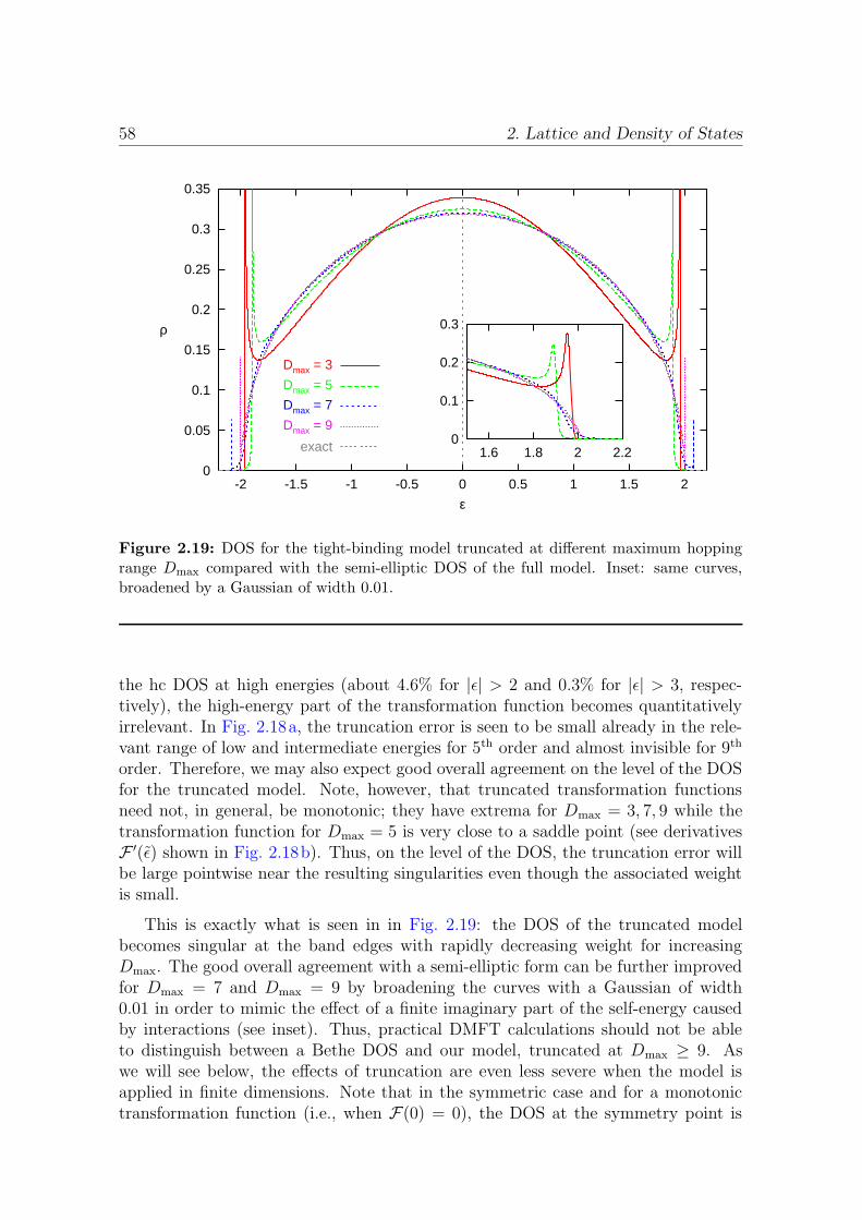
58 2. Lattice and Density of States
0
0.05
0.1
0.15
0.2
0.25
0.3
0.35
-2 -1.5 -1 -0.5 0 0.5 1 1.5 2
ρ
ε
Dmax = 3
Dmax = 5
Dmax = 7
Dmax = 9
exact 0
0.1
0.2
0.3
1.6 1.8 2 2.2
Figure 2.19: DOS for the tight-binding model truncated at different maximum hoppingrange Dmax compared with the semi-elliptic DOS of the full model. Inset: same curves,broadened by a Gaussian of width 0.01.
the hc DOS at high energies (about 4.6% for |ε| > 2 and 0.3% for |ε| > 3, respec-tively), the high-energy part of the transformation function becomes quantitativelyirrelevant. In Fig. 2.18a, the truncation error is seen to be small already in the rele-vant range of low and intermediate energies for 5th order and almost invisible for 9th
order. Therefore, we may also expect good overall agreement on the level of the DOSfor the truncated model. Note, however, that truncated transformation functionsneed not, in general, be monotonic; they have extrema for Dmax = 3, 7, 9 while thetransformation function for Dmax = 5 is very close to a saddle point (see derivativesF ′(ε) shown in Fig. 2.18b). Thus, on the level of the DOS, the truncation error willbe large pointwise near the resulting singularities even though the associated weightis small.
This is exactly what is seen in in Fig. 2.19: the DOS of the truncated modelbecomes singular at the band edges with rapidly decreasing weight for increasingDmax. The good overall agreement with a semi-elliptic form can be further improvedfor Dmax = 7 and Dmax = 9 by broadening the curves with a Gaussian of width0.01 in order to mimic the effect of a finite imaginary part of the self-energy causedby interactions (see inset). Thus, practical DMFT calculations should not be ableto distinguish between a Bethe DOS and our model, truncated at Dmax ≥ 9. Aswe will see below, the effects of truncation are even less severe when the model isapplied in finite dimensions. Note that in the symmetric case and for a monotonictransformation function (i.e., when F(0) = 0), the DOS at the symmetry point is
2.4. Redefinition of the Bethe Lattice 59
fully determined by the first derivative of the transformation function at the origin,
1
ρ(ε = 0)=√
2πF ′(0) =√
2π∞∑
n=0
t∗2n+1(−1)n(2n+ 1)!!√
(2n+ 1)!. (2.71)
This series is quickly converging for the tight-binding model corresponding to a BetheDOS as seen in Fig. 2.18 and Fig. 2.19.29
2.4.3 Finite Dimensionality
After having verified that the properties of the tight-binding model with semi-ellipticDOS derived in this section are robust with respect to truncation, we can now studythe robustness with respect to application in finite dimensions and thereby distin-guish generic from more artificial features. For this purpose, we explicitly calculatethe dispersion for the redefined Bethe model [i.e., the model defined by (2.68)], trun-cated at 3rd or 5th order hopping. Here, we evaluate BD(k) as defined in (2.48)without resorting to any large-d approximations for the involved sums or the num-ber of equivalent hopping terms; in particular, the approximation in (2.44) is notused.30 In the necessary summations, the exclusion of terms with equal indices posesa combinatorial problem which can be solved iteratively or as a linear system ofequations. In order to illustrate the basic considerations, we show how the sum-mation restrictions are replaced for D = 2, 3:
∑
i6=j =∑
ij (1− δij) ;∑
i6=j 6=k =∑
ijk (1− δij − δik − δjk + 2δijk), where the generalized δ-function equals 1 if all in-dices are equal and is 0 otherwise. For the sake of brevity, we will in the followingstate the results for AD(k) := (2/d)−d/2BD(k), from which the exact d-dimensionaldispersion can be obtained in the form
εD(k) = t∗D2D/2
D!√(dD
)AD(k) (2.72)
and which agrees with (2.47) in the limit dÀ D. The coefficient functions read
A1(k) =d∑
α=1
cos(kα); A2(k) =(∑
α
cos(kα))2
−∑
α
cos2(kα)
29Note that a gapped DOS as in the case of the flat band DOS considered above can only arisewhen the sum in (2.71) diverges which means that the hopping matrix elements t∗n decay moreslowly than n−5/4.
30We keep, however, the selection of hopping terms defined at the beginning of this section, i.e.,do not consider extended hopping along the cartesic axes.
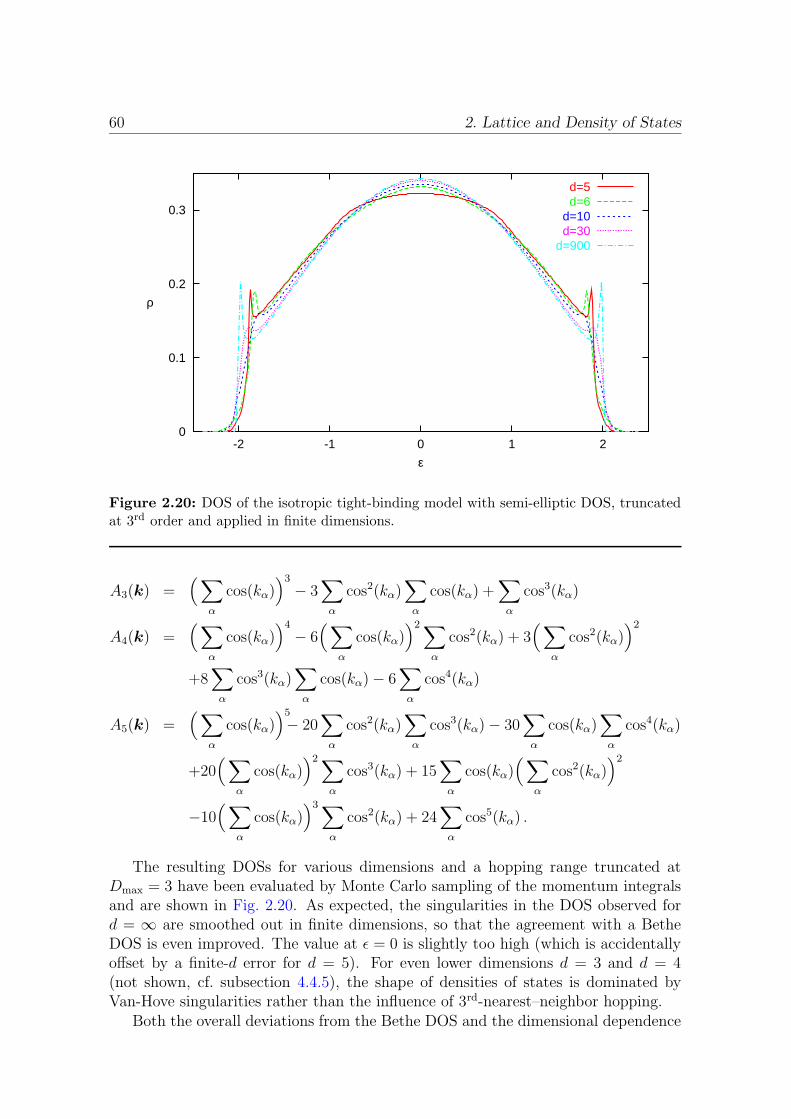
60 2. Lattice and Density of States
0
0.1
0.2
0.3
-2 -1 0 1 2
ρ
ε
d=5d=6
d=10d=30
d=900
Figure 2.20: DOS of the isotropic tight-binding model with semi-elliptic DOS, truncatedat 3rd order and applied in finite dimensions.
A3(k) =(∑
α
cos(kα))3
− 3∑
α
cos2(kα)∑
α
cos(kα) +∑
α
cos3(kα)
A4(k) =(∑
α
cos(kα))4
− 6(∑
α
cos(kα))2∑
α
cos2(kα) + 3(∑
α
cos2(kα))2
+8∑
α
cos3(kα)∑
α
cos(kα)− 6∑
α
cos4(kα)
A5(k) =(∑
α
cos(kα))5
− 20∑
α
cos2(kα)∑
α
cos3(kα)− 30∑
α
cos(kα)∑
α
cos4(kα)
+20(∑
α
cos(kα))2∑
α
cos3(kα) + 15∑
α
cos(kα)(∑
α
cos2(kα))2
−10(∑
α
cos(kα))3∑
α
cos2(kα) + 24∑
α
cos5(kα) .
The resulting DOSs for various dimensions and a hopping range truncated atDmax = 3 have been evaluated by Monte Carlo sampling of the momentum integralsand are shown in Fig. 2.20. As expected, the singularities in the DOS observed ford = ∞ are smoothed out in finite dimensions, so that the agreement with a BetheDOS is even improved. The value at ε = 0 is slightly too high (which is accidentallyoffset by a finite-d error for d = 5). For even lower dimensions d = 3 and d = 4(not shown, cf. subsection 4.4.5), the shape of densities of states is dominated byVan-Hove singularities rather than the influence of 3rd-nearest–neighbor hopping.
Both the overall deviations from the Bethe DOS and the dimensional dependence
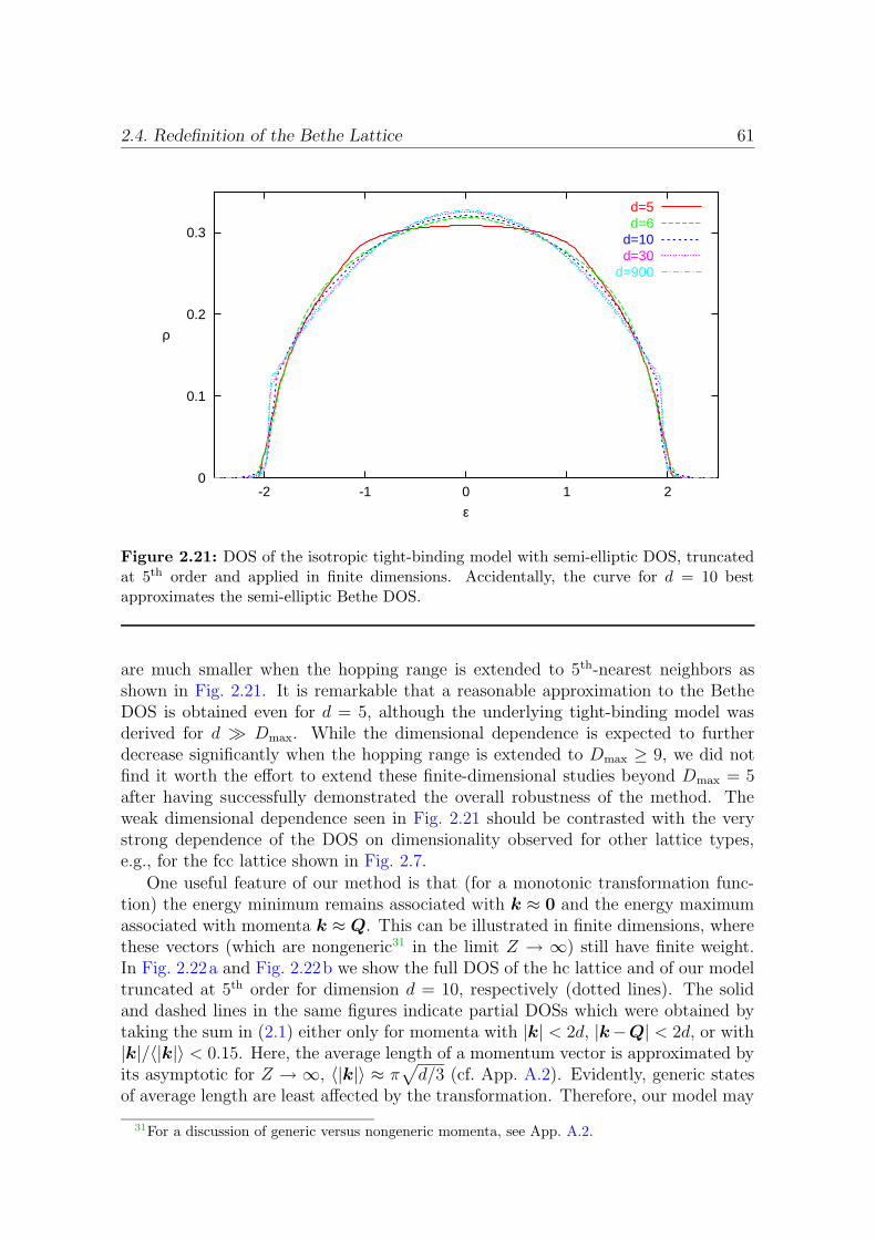
2.4. Redefinition of the Bethe Lattice 61
0
0.1
0.2
0.3
-2 -1 0 1 2
ρ
ε
d=5d=6
d=10d=30
d=900
Figure 2.21: DOS of the isotropic tight-binding model with semi-elliptic DOS, truncatedat 5th order and applied in finite dimensions. Accidentally, the curve for d = 10 bestapproximates the semi-elliptic Bethe DOS.
are much smaller when the hopping range is extended to 5th-nearest neighbors asshown in Fig. 2.21. It is remarkable that a reasonable approximation to the BetheDOS is obtained even for d = 5, although the underlying tight-binding model wasderived for d À Dmax. While the dimensional dependence is expected to furtherdecrease significantly when the hopping range is extended to Dmax ≥ 9, we did notfind it worth the effort to extend these finite-dimensional studies beyond Dmax = 5after having successfully demonstrated the overall robustness of the method. Theweak dimensional dependence seen in Fig. 2.21 should be contrasted with the verystrong dependence of the DOS on dimensionality observed for other lattice types,e.g., for the fcc lattice shown in Fig. 2.7.
One useful feature of our method is that (for a monotonic transformation func-tion) the energy minimum remains associated with k ≈ 0 and the energy maximumassociated with momenta k ≈ Q. This can be illustrated in finite dimensions, wherethese vectors (which are nongeneric31 in the limit Z → ∞) still have finite weight.In Fig. 2.22a and Fig. 2.22b we show the full DOS of the hc lattice and of our modeltruncated at 5th order for dimension d = 10, respectively (dotted lines). The solidand dashed lines in the same figures indicate partial DOSs which were obtained bytaking the sum in (2.1) either only for momenta with |k| < 2d, |k−Q| < 2d, or with|k|/〈|k|〉 < 0.15. Here, the average length of a momentum vector is approximated byits asymptotic for Z → ∞, 〈|k|〉 ≈ π
√
d/3 (cf. App. A.2). Evidently, generic statesof average length are least affected by the transformation. Therefore, our model may
31For a discussion of generic versus nongeneric momenta, see App. A.2.

62 2. Lattice and Density of States
a) b)
0
0.1
0.2
0.3
-4 -3 -2 -1 0 1 2 3 4
ρ
ε
k~0generic k
k~Qall k
0
0.1
0.2
0.3
-3 -2 -1 0 1 2 3
ρ
ε
k~0generic k
k~Qall k
Figure 2.22: Partial DOSs a) of the hc lattice and b) of the 5th order truncation of theredefined Bethe lattice in d = 10 (solid and dashed lines) in comparison with the full DOSs(dotted lines). The restriction to momenta with |k| ≈ 0, |k| ≈ 〈|k|〉, and |k −Q| ≈ 0 isexplained in the text.
be regarded as a minimal modification of the NN-hopping hc lattice for which theDOS becomes semi-elliptic.
2.4.4 Application to Asymmetric Model DOS
It should be evident that our method is by no means restricted to the Bethe DOS or toa symmetric DOS in general. In fact, it gives a natural description for all nonsingularsingle-band DOSs. In order to illustrate the application to an asymmetric case, todraw a connection to earlier work (Wahle et al., 1998), and to compare with estimatesfor hopping amplitudes obtained within an alternative scheme (Kollar, 1998), wealso applied our formalism to the asymmetric model DOS (2.27) which contains theasymmetry parameter −1 ≤ a ≤ 1 and coincides with the semi-elliptic Bethe DOSfor a = 0.
As seen in Table 2.2, slight asymmetry (a = 0.5) leaves the scaled hopping matrixelements corresponding to odd hopping range D = 2n + 1 almost invariant whilethe even range hopping becomes relevant. The energy shift (i.e., finite first mo-ment) implicit in (2.27) for |a| > 0 gives rise to a finite on-site amplitude t20 whichcan be evaluated using (2.55) for D = 0 just like for finite hopping range D > 0.With increasing asymmetry (a = 0.9 and a = 0.98, cf. Fig. 2.13), the even rangehopping elements become more dominant and also the decay is slower than for thesymmetric Bethe DOS. Even an asymmetry (a = 0.98) strong enough to allow forferromagnetism in the pure Hubbard model (Wahle et al., 1998) thus naturally fitsinto the present scheme. However, an application of the method (with a monotonictransformation function) would be questionable for the singular case a = 1, which

2.4. Redefinition of the Bethe Lattice 63
a = 0.5 a = 0.9 a = 0.98
D t∗D∑D
n=1 t∗n2 t∗D
∑Dn=1 t
∗n2 t∗D
∑Dn=1 t
∗n2
0 -0.26795 0.000000 -0.62679 0.000000 -0.81735 0.000000
1 0.98364 0.967540 0.96671 0.934524 0.95139 0.9051412 0.08255 0.974354 0.19413 0.972212 0.25457 0.9699453 -0.15137 0.997267 -0.14143 0.992213 -0.13252 0.9875054 -0.03143 0.998255 -0.07444 0.997755 -0.09835 0.9971775 0.03775 0.999680 0.03236 0.998802 0.02759 0.9979386 0.01273 0.999842 0.03046 0.999730 0.04063 0.9995897 -0.01062 0.999955 -0.00776 0.999790 -0.00528 0.9996178 -0.00534 0.999983 -0.01294 0.999957 -0.01748 0.9999239 0.00310 0.999993 0.00160 0.999960 0.00032 0.999923
10 0.00229 0.999998 0.00566 0.999992 0.00777 0.99998311 -0.00091 0.999999 -0.00012 0.999992 0.00053 0.99998312 -0.00101 1.000000 -0.00253 0.999998 -0.00355 0.99999613 0.00024 1.000000 -0.00018 0.999998 -0.00050 0.99999614 0.00045 1.000000 0.00116 1.000000 0.00167 0.99999915 -0.00006 1.000000 0.00016 1.000000 0.00032 0.999999
Table 2.2: Leading hopping matrix elements corresponding to the generalized asymmetricmodel DOS (2.27) with parameter a (cf. Table 2.1). The columns which consist of partialsums indicate rapid convergence of the corresponding dispersion and DOS: only a fraction1−
∑Dn=1 t
∗n2 of the variance arises from hopping terms beyond Dth neighbors. The “hop-
ping” term with range D = 0 denotes an on-site energy, i.e., the first moment of the energydistribution.
corresponds to a Bethe lattice with only NNN hopping, as we have shown in Sec. 2.2.We would have to overcome numerical stability issues just to reproduce a square-root singularity at the lower band edge which we regard as an artifact of d =∞ (incomplete analogy to the situation for the fcc lattice).
Earlier attempts to link the asymmetric model DOS (2.27) to some microscopictight-binding model (Wahle et al., 1998; Kollar, 1998) have led to a related, but quitedifferent construction scheme, which can be applied in low and infinite dimensions(Kollar, 2002). The straightforward application in d = 1 to the DOS (2.27) witha = 0.98 yields scaled hopping matrix elements which are well approximated byt∗2n+1 = 0.67 (2n)−1.6, t∗2n = −0.54 (2n)−1.6 for small hopping range and decay astD ∼ D−5/3 for large range (Kollar, 1998). When generalized to higher dimensions,Kollar’s construction is based on a dispersion ε(k) = g(|k|) (for some function g)which is spherical except at the boundaries of the Brillouin zone. We regard it moreas a proof of existence of a dispersion for a given DOS in arbitrary dimension than asa workable scheme for the following reasons: Most importantly, the above sphericalform for the dispersion implies discontinuities in the Fermi velocity at the boundariesof the Brillouin zone for d > 1 which, if taken seriously, makes the computation of
64 2. Lattice and Density of States
transport properties pointless. Due to the violation of symmetry between k = 0 andk = Q, concepts like perfect nesting become meaningless. Additionally, the hoppingis dominantly along the axes and is very slowly decaying (as tD ∼ D−2, only slightlyfaster than in the one-dimensional case). Thus, our approach appears much morephysical in higher dimensions which is not surprising since it was derived for thelarge-d limit.32
2.5 Conclusion
In this chapter, we have carefully studied the relationships between lattice types,densities of states, and magnetic frustration in high dimensions. Evaluating Brillouin-zone integrals by Monte Carlo sampling, we have computed the (noninteracting) DOSof the hypercubic lattice with hopping to nearest and/or next-nearest neighbors aswell as the DOS of the hyperdiamond lattice (see App. B) in low, intermediate, andhigh dimensions. Thereby and by comparing with the corresponding analytical d =∞results we have distinguished generic features from features that are artifacts of thed = ∞ limit. In particular, we have established that for regular lattices, magneticfrustration is generically associated with an asymmetric DOS or with off-diagonaldisorder.
We have then characterized the Bethe “lattice” which is a tree in the sense ofgraph theory rather than a regular lattice. We have pointed out that a semi-ellipticDOS implies the absence or cancellation of all self-avoiding loops in a renormal-ized perturbation expansion for any lattice. By computing moments of the DOSof the Bethe lattice with hopping to nearest and next-nearest neighbors (NNN), wehave contradicted an earlier claim that NNN hopping should leave the DOS invari-ant. Furthermore, we have presented the first (analytic) calculation of the (stronglyasymmetric) DOS of the Bethe lattice with only NNN hopping.
We have developed a general method of constructing a tight-binding Hamiltonianwhich yields a given, arbitrary DOS in the limit of infinite dimensions. This methodallows for the computation of all physical quantities that can be defined for thecorresponding finite-dimensional model. Such a method is particularly useful in thecontext of the DMFT, where nonlocal properties can be derived by combining anessentially local property of the interacting system with a nonlocal property of thenoninteracting system. Examples for such properties are the optical conductivity(which we will consider in chapter 4) and susceptibilities.
By applying the new general-dispersion formalism to the semi-elliptic “Bethe”DOS, we have found the first regular lattice with a bounded DOS in high dimensions,thereby removing one of the major artifacts previously regarded as inherent to thelimit d → ∞. We have verified that versions of this model with truncated hoppingranges still give reasonable descriptions. While the DOS is then no longer strictlybounded, the weight associated with long-frequency tails is suppressed exponentiallywith the number of hopping terms and becomes negligible for numerical purposes
32In contrast, only Kollar’s construction can be applied in very low dimensions, in particular inone dimension where it becomes exact.
2.5. Conclusion 65
when hopping to 7th or 9th nearest neighbors is included. For the full model, theaverage squared hopping distance is 1.054, i.e., surprisingly close to the value 1 validfor the usual hypercubic lattice. The convergence of the method (with the number ofnonzero hopping matrix elements and with dimensionality) is similarly good in termsof the distribution of spectral weight for other sufficiently smooth target DOSs. Thefact that exactly vanishing even-range hopping matrix elements are predicted for anysymmetric DOS follows necessarily for any consistent approach and is not specific toour method.
With the general dispersion method developed in Sec. 2.3, we have singled outone route to high dimensions with a series of very favorable properties (specializingon the case of a monotonic transformation function): (i) The approach does not re-quire large long-range hopping amplitudes. (ii) Generically, the DOSs correspondingto finite-d versions of the computed tight-binding model depend only weakly on di-mensionality. (iii) The topology of the Fermi surface remains hypercubic-like at allfillings in arbitrary dimensions with the energy minimum of εk at k = 0 (and themaximum at k = Q). (iv) The full hypercubic symmetry is retained. (v) For the firsttime, transport properties for the Bethe DOS can be calculated in a fully consistentway (including an f -sum rule) without resorting to anisotropic models. (vi) Thederived equations can be used as a heuristic approach for transport calculations infinite dimensions when only the DOS is known (e.g., from LDA calculations).

66 2. Lattice and Density of States
67
Chapter 3
Mott Metal-Insulator Transition inthe d → ∞ Hubbard Model
One of the most fascinating phenomena of strongly correlated electron systems is theinteraction-induced metal-insulator transition. Such a transition is fundamentallydifferent from filling-induced transitions between metals and band insulators since itcannot be understood in terms of (effectively) noninteracting electrons. Particularlychallenging is the Mott transition, the interaction-induced transition between a para-magnetic metal (PM) and a paramagnetic insulator (PI).1 As this transition does notbreak the translational symmetry of the lattice, its description needs to take strongelectronic correlations into account. For this reason, proximity to a Mott transitionmay be even regarded as a defining property of strongly correlated electron systems.The explanation and modeling of the Mott transition is a long-standing importantand difficult problem of condensed matter physics (Mott, 1968; Mott, 1990; Geb-hard, 1997; Imada, Fujimori, and Tokura, 1998).
In this chapter, we present studies of the Mott metal-insulator transition (MIT)occurring in the infinite-dimensional half-filled Hubbard model. Specifically, resultswill be obtained for the Bethe lattice, i.e., for a semi-elliptic noninteracting DOS.In order to observe the transition of interest in the paramagnetic phase, antiferro-magnetism is suppressed in the calculation, which corresponds to treating the latticeas fully frustrated. For this model, the Mott transition occurs for an interactionU slightly larger than the bandwidth W (see below). Consequently, perturbativemethods are not adequate for its description and may only a posteriori be useful forcomparison. We will argue later that even numerically exact methods such as QMCor ED may become problematic in the transition region if not used with great care.In fact, one of the achievements of this thesis is the settlement of a controversy aboutthe qualitative shape of the MIT phase diagram of the specified model. Therefore,our treatment will have to at least partially follow the historical development.
In Sec. 3.1 we give an experimental motivation and discuss the applicability ofthe model. In Sec. 3.2, we discuss strategies for pinpointing and characterizing phase
1Interactions can alternatively drive the transition of a metal into an insulating ordered state,namely an antiferromagnetic Neel low-temperature phase (AFI); the AFI, however, may be under-stood as an effective band insulator in the halved Brillouin zone (see subsection 1.1.4).

68 3. Mott Metal-Insulator Transition in the d→∞ Hubbard Model
transitions within the DMFT and specify potentially useful observables. A first lookat the history of the phase diagram is given in Sec. 3.3 where it will be seen that earlyQMC studies collaboratively performed in this work correctly captured some aspectsof the phase diagram while failing in describing others. In Sec. 3.4, we explainthe reasons for this failure and correct a fundamental problem of the QMC codepreviously used within our group. In addition, we quantify the remaining numericalerrors and present further improvements of the QMC algorithm and code developedas part of this thesis.
Accurate phase boundaries are then determined in Sec. 3.5. Here, we show thatthe total internal energy (per site) is best suited for distinguishing metallic from in-sulating solutions, in particular in the extrapolation ∆τ → 0. The resulting phasediagram is constructed and the controversy resolved in subsection 3.5.4. The obser-vation of a coexistence region of metallic and insulating solutions generates the needto determine the true thermodynamic phase transition line using free energy infor-mation. Prior to this work, this task had seemed too complicated to be accomplishedon the basis of numerically exact techniques; even in the context of iterative pertur-bation theory, results for this line had been contradictory. Using newly developedschemes, we demonstrate in Sec. 3.6 how the first order phase transition line canbe located based on QMC simulations; using low-temperature thermodynamic infor-mation and well-established numerical zero-temperature results, the thermodynamicphase transition line is even extended down to zero temperature. The presentation ofthe full phase diagram in subsection 3.6.3 is supplemented by a discussion of possiblescenarios for partially frustrated models in subsection 3.6.4.
Implications of the Landau theory of phase transitions for the convergence ofthe DMFT iteration process and the suitability of the fitting functions introduced inSec. 3.5 are discussed in Sec. 3.7. In addition, we propose a new concept for computingfree energy differences by solving impurity models which are (in general) not solutionsof the DMFT equations. In the final section 3.8, local spectral functions are computedusing the maximum entropy method. These results provide additional insight in thenature of the phase transition and will later be needed for the computation of theoptical conductivity in chapter 4.
3.1 Motivation
3.1.1 Experiment
Experimentally, metal-insulator transitions may be observed upon variation of tem-perature and pressure for a given sample or as a function of doping within a classof materials. Since the induced variations of energy scales are relatively small, onlyfew classes of materials, such as the oxides of vanadium, titanium, and chrome aswell as NiSe2−xSx display a correlation-induced MIT (Heine and Mattheiss, 1971;Mattheiss, 1972; Mott, 1990). The compound La1-xSrxTiO3, which will be treatedwithin LDA+DMFT in chapter 5, falls into this group; among the most promi-nent and best characterized examples, however, is V2O3 (Rice and McWhan, 1970;McWhan, Remeika, Rice, Brinkman, Maita, and Menth, 1971; McWhan, Remeika,
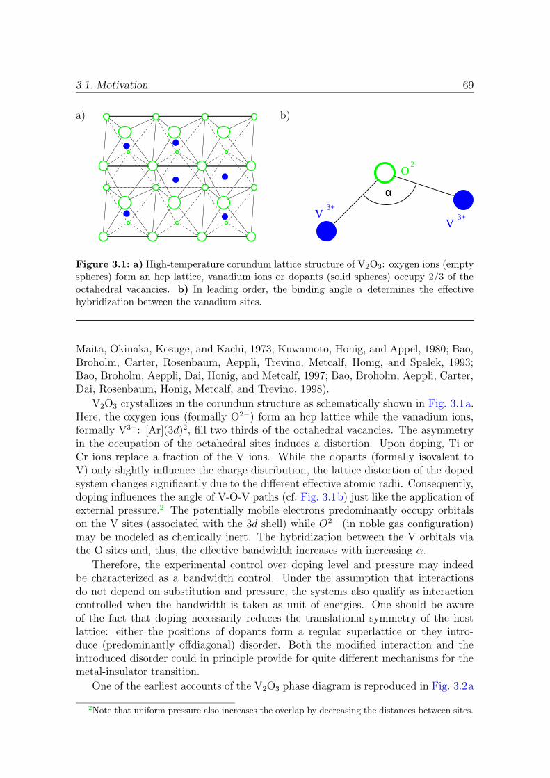
3.1. Motivation 69
a) b)
O2-
α
V3+
V3+
Figure 3.1: a) High-temperature corundum lattice structure of V2O3: oxygen ions (emptyspheres) form an hcp lattice, vanadium ions or dopants (solid spheres) occupy 2/3 of theoctahedral vacancies. b) In leading order, the binding angle α determines the effectivehybridization between the vanadium sites.
Maita, Okinaka, Kosuge, and Kachi, 1973; Kuwamoto, Honig, and Appel, 1980; Bao,Broholm, Carter, Rosenbaum, Aeppli, Trevino, Metcalf, Honig, and Spalek, 1993;Bao, Broholm, Aeppli, Dai, Honig, and Metcalf, 1997; Bao, Broholm, Aeppli, Carter,Dai, Rosenbaum, Honig, Metcalf, and Trevino, 1998).
V2O3 crystallizes in the corundum structure as schematically shown in Fig. 3.1a.Here, the oxygen ions (formally O2−) form an hcp lattice while the vanadium ions,formally V3+: [Ar](3d)2, fill two thirds of the octahedral vacancies. The asymmetryin the occupation of the octahedral sites induces a distortion. Upon doping, Ti orCr ions replace a fraction of the V ions. While the dopants (formally isovalent toV) only slightly influence the charge distribution, the lattice distortion of the dopedsystem changes significantly due to the different effective atomic radii. Consequently,doping influences the angle of V-O-V paths (cf. Fig. 3.1b) just like the application ofexternal pressure.2 The potentially mobile electrons predominantly occupy orbitalson the V sites (associated with the 3d shell) while O2− (in noble gas configuration)may be modeled as chemically inert. The hybridization between the V orbitals viathe O sites and, thus, the effective bandwidth increases with increasing α.
Therefore, the experimental control over doping level and pressure may indeedbe characterized as a bandwidth control. Under the assumption that interactionsdo not depend on substitution and pressure, the systems also qualify as interactioncontrolled when the bandwidth is taken as unit of energies. One should be awareof the fact that doping necessarily reduces the translational symmetry of the hostlattice: either the positions of dopants form a regular superlattice or they intro-duce (predominantly offdiagonal) disorder. Both the modified interaction and theintroduced disorder could in principle provide for quite different mechanisms for themetal-insulator transition.
One of the earliest accounts of the V2O3 phase diagram is reproduced in Fig. 3.2a
2Note that uniform pressure also increases the overlap by decreasing the distances between sites.
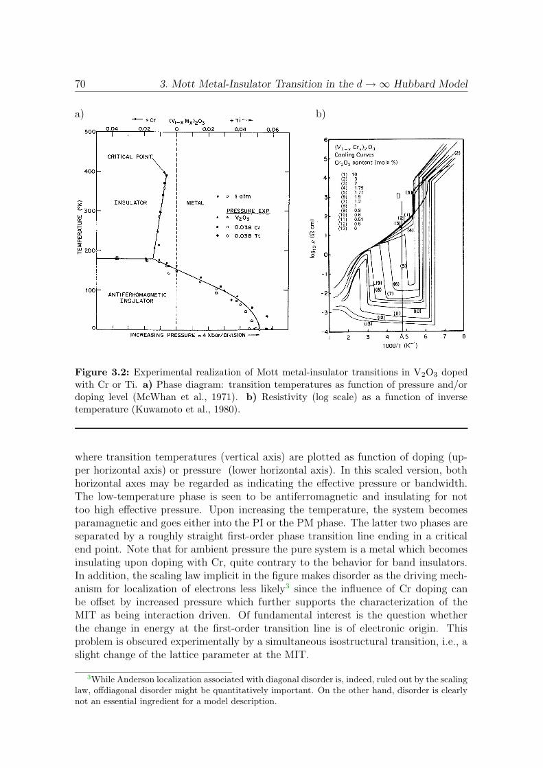
70 3. Mott Metal-Insulator Transition in the d→∞ Hubbard Model
a) b)
(d1-d2LI ) hybridization (Uozumi et al., 1993). Cluster-model analysis has revealed considerable weight ofcharge-transfer configurations, d3LI ,d4LI 2, . . . , mixed intothe ionic d2 configuration, resulting in a net d-electronnumber of nd.3.1 (Bocquet et al., 1996). This value isconsiderably larger than the d-band filling or the formald-electron number n52 and is in good agreement withthe value (nd53.0) deduced from an analysis of core-core-valence Auger spectra (Sawatzky and Post, 1979).If the above local-cluster CI picture is relevant to experi-ment, the antibonding counterpart of the split-off bond-ing state is predicted to be observed as a satellite on thehigh-binding-energy side of the O 2p band, although itsspectral weight may be much smaller than the bondingstate [due to interference between the d2→d1
1e andd3LI →d2LI 1e photoemission channels; see Eq. (3.12)].Such a spectral feature was indeed observed in an ultra-violet photoemission study by Smith and Henrich (1988)and in a resonant photoemission study by Park andAllen (1997). In spite of the strong p-d hybridizationand the resulting charge-transfer satellite mechanism de-scribed above, it is not only convenient but also realisticto regard the d1-d2LI bonding band as an effective V 3dband (lower Hubbard band). The 3d wave function isthus considerably hybridized with oxygen p orbitals andhence has a relatively small effective U of 1–2 eV (Sa-watzky and Post, 1979) instead of the bare value U;4 eV. Therefore the effective d bandwidth W becomescomparable to the effective U : W;U . With these factsin mind, one can regard V2O3 as a model Mott-Hubbardsystem and the (degenerate) Hubbard model as a rel-evant model for analyzing the physical properties ofV2O3.
The time-honored phase diagram for doped V2O3 sys-tems, (V12xCrx)2O3 and (V12xTix)2O3 , is reproducedin Fig. 70. The phase boundary represented by the solidline is of first order, accompanied by thermal hysteresis(Kuwamoto, Honig, and Appel, 1980). In a Cr-dopedsystem (V12xCrx)2O3 , a gradual crossover is observedfrom the high-temperature paramagnetic metal (PM) to
FIG. 69. Photoemission spectra of V2O3 in the metallic phasetaken using photon energies in the 3p-3d core excitation re-gion. From Shin et al., 1990.
FIG. 68. Corundum structure of V2O3.
FIG. 70. Phase diagram for doped V2O3 systems,(V12xCrx)2O3 and (V12xTix)2O3. From McWhan et al., 1971,1973.
1147Imada, Fujimori, and Tokura: Metal-insulator transitions
Rev. Mod. Phys., Vol. 70, No. 4, October 1998
Figure 3.2: Experimental realization of Mott metal-insulator transitions in V2O3 dopedwith Cr or Ti. a) Phase diagram: transition temperatures as function of pressure and/ordoping level (McWhan et al., 1971). b) Resistivity (log scale) as a function of inversetemperature (Kuwamoto et al., 1980).
where transition temperatures (vertical axis) are plotted as function of doping (up-per horizontal axis) or pressure (lower horizontal axis). In this scaled version, bothhorizontal axes may be regarded as indicating the effective pressure or bandwidth.The low-temperature phase is seen to be antiferromagnetic and insulating for nottoo high effective pressure. Upon increasing the temperature, the system becomesparamagnetic and goes either into the PI or the PM phase. The latter two phases areseparated by a roughly straight first-order phase transition line ending in a criticalend point. Note that for ambient pressure the pure system is a metal which becomesinsulating upon doping with Cr, quite contrary to the behavior for band insulators.In addition, the scaling law implicit in the figure makes disorder as the driving mech-anism for localization of electrons less likely3 since the influence of Cr doping canbe offset by increased pressure which further supports the characterization of theMIT as being interaction driven. Of fundamental interest is the question whetherthe change in energy at the first-order transition line is of electronic origin. Thisproblem is obscured experimentally by a simultaneous isostructural transition, i.e., aslight change of the lattice parameter at the MIT.
3While Anderson localization associated with diagonal disorder is, indeed, ruled out by the scalinglaw, offdiagonal disorder might be quantitatively important. On the other hand, disorder is clearlynot an essential ingredient for a model description.
3.1. Motivation 71
Figure 3.2b shows the resistivity as a function of inverse temperature for variouslevels of Cr doping. The lowest curve corresponds to the pure case, i.e., the verticaldashed line in the phase diagram Fig. 3.2a. This curve displays only one kink, asharp increase of the resistivity by 7 orders of magnitude at the Neel temperature.For sufficiently large doping, a second jump by some 2 or 3 orders of magnitudeappears at higher temperature (i.e., going left in the plot) which indicates the Mottmetal-insulator transition which is the subject of interest within this chapter.
3.1.2 Theory
A theoretical description of the V2O3 phase diagram should at least reproduce itstopology including the first-order Mott transition line. If such a description couldbe found in terms of a purely electronic model, this would be a strong indication forelectronic correlations being the driving force behind the Mott transition. Latticedegrees of freedom would, then, appear less important in this respect. While orbitaldegrees of freedom certainly play an important role for V2O3, at least quantitatively[see Held, Keller, Eyert, Vollhardt, and Anisimov (2001) and references therein], thevery essence of the Mott transition may already be captured qualitatively by thehalf-filled single-band Hubbard model. This model is a likely candidate since itsparamagnetic phase is a (perfect) metal for U = 0 and an insulator for U = ∞. Atransition would be expected for U ≈ W if W is an appropriate measure of the freebandwidth. For the usually considered case of NN hopping on a bipartite lattice,however, the antiferromagnetic phase generically extends to high enough tempera-tures that the evolution from metal to insulator as a function of U should occur asa smooth crossover. This expectation is indeed an established fact for the Bethelattice as well as for the hc lattice with NN hopping in infinite dimensions (see be-low) and is supported by recent QMC results for the simple cubic lattice in d = 3(Staudt, Dzierzawa, and Muramatsu, 2000). Therefore, the Mott transition can onlybe studied on the Hubbard model when the antiferromagnetic phase is suppressed.
The natural microscopic method of modeling magnetic frustration is the inclu-sion of hopping terms to (at least) next-nearest neighbors. As discussed in chapter2, frustration then generically implies an asymmetric DOS. DMFT results for thehypercubic lattice with NN and NNN hopping are shown in Fig. 3.3a. Here, symbolsand interpolating lines indicate the Neel temperature as computed using QMC foran increasing degree of frustration from top to bottom (Schlipf, 1998). Alternatively,antiferromagnetism may be suppressed in analytical and in mean-field methods4 byrestricting solutions to the subspace with appropriate symmetries. For the semi-elliptic Bethe DOS, this choice corresponds, e.g., to solving a fully disordered modelwhere the hopping terms obey 〈tij〉 = 0 and 〈t2ij〉 = t∗2/Z (cf. subsection 2.2.2). Thephase diagram of this “fully frustrated Bethe lattice” is shown in Fig. 3.3b as ob-tained by Georges et al. (1996) within iterated perturbation theory (IPT). Accordingto this result, metallic and insulating solutions coexist at low temperatures over a
4Such a suppression is not possible in the context of QMC applied directly in finite dimensions.For this method, the inclusion of NNN is not a practical alternative since it leads to the minus-signproblem. Therefore, finite-dimensional QMC can hardly treat frustration at all.
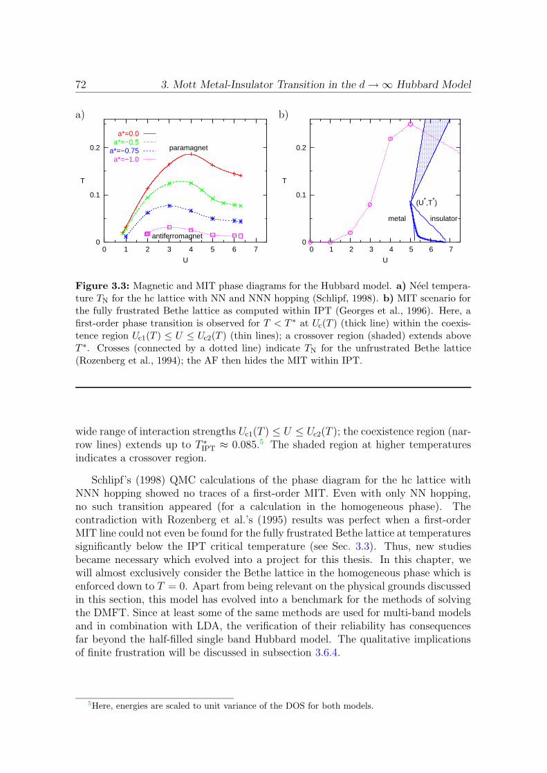
72 3. Mott Metal-Insulator Transition in the d→∞ Hubbard Model
a) b)
0
0.1
0.2
0 1 2 3 4 5 6 7
T
U
antiferromagnet
paramagnet
a*=0.0a*=−0.5
a*=−0.75a*=−1.0
0
0.1
0.2
0 1 2 3 4 5 6 7
T
U
(U*,T*)
metal insulator
Figure 3.3: Magnetic and MIT phase diagrams for the Hubbard model. a) Neel tempera-ture TN for the hc lattice with NN and NNN hopping (Schlipf, 1998). b) MIT scenario forthe fully frustrated Bethe lattice as computed within IPT (Georges et al., 1996). Here, afirst-order phase transition is observed for T < T ∗ at Uc(T ) (thick line) within the coexis-tence region Uc1(T ) ≤ U ≤ Uc2(T ) (thin lines); a crossover region (shaded) extends aboveT ∗. Crosses (connected by a dotted line) indicate TN for the unfrustrated Bethe lattice(Rozenberg et al., 1994); the AF then hides the MIT within IPT.
wide range of interaction strengths Uc1(T ) ≤ U ≤ Uc2(T ); the coexistence region (nar-row lines) extends up to T ∗
IPT ≈ 0.085.5 The shaded region at higher temperaturesindicates a crossover region.
Schlipf’s (1998) QMC calculations of the phase diagram for the hc lattice withNNN hopping showed no traces of a first-order MIT. Even with only NN hopping,no such transition appeared (for a calculation in the homogeneous phase). Thecontradiction with Rozenberg et al.’s (1995) results was perfect when a first-orderMIT line could not even be found for the fully frustrated Bethe lattice at temperaturessignificantly below the IPT critical temperature (see Sec. 3.3). Thus, new studiesbecame necessary which evolved into a project for this thesis. In this chapter, wewill almost exclusively consider the Bethe lattice in the homogeneous phase which isenforced down to T = 0. Apart from being relevant on the physical grounds discussedin this section, this model has evolved into a benchmark for the methods of solvingthe DMFT. Since at least some of the same methods are used for multi-band modelsand in combination with LDA, the verification of their reliability has consequencesfar beyond the half-filled single band Hubbard model. The qualitative implicationsof finite frustration will be discussed in subsection 3.6.4.
5Here, energies are scaled to unit variance of the DOS for both models.

3.2. Characterization of Phase Transitions within the DMFT 73
3.2 Characterization of Phase Transitions within
the DMFT
In this section, we will discuss how phase transitions can be found and character-ized within the DMFT. In subsection 3.2.1, we focus on the general implications ofthe mean-field character of the DMFT in connection with first-order transitions. Aparticularly important aspect is the question how the numerical stability of solutionsin the iterative process is related to their thermodynamic (meta-) stability. Thisproblem had been neglected in the literature so far and is now solved for a particulariteration scheme in subsection 3.2.2. Finally, we collect useful observables and discusstheir general behavior in subsection 3.2.3.
3.2.1 Transitions of First or Higher Order
In a thermal statistical ensemble, properties such as the (free) energy per particle,average filling, or average double occupancy are defined in terms of traces over allpossible states. Therefore, the observables are well-defined functions of a complete setof external parameters; for the Hubbard model on a given lattice (with unit varianceof the DOS) these parameters are the on-site interaction U , the temperature T , andthe chemical potential µ. More precisely, the free energy F is a continuous functionwhile its derivatives may be discontinuous at some hypersurfaces, i.e., lines in a 2-dimensional subspace of parameters such as U and T . The discontinuities indicate aphase transition; according to Ehrenfest, the order of the transition is defined as theorder of the first discontinuous derivative of F . In principle, the search for a phasetransition is, therefore, straightforward: sweeping through the parameter space, onesearches for jumps or kinks in the derivatives of F with respect to U or T , i.e., thedouble occupancy D or (minus) the entropy S or related observables. This is theusual practice, e.g., for QMC in finite dimensions.6
In contrast, in mean-field theories such as the DMFT, the ensemble average isperformed with the mean-field [here G(iωn), cf. subsection 1.2.3] as an additionalparameter which has to be determined self-consistently. The resulting fixed pointproblem may have one or more solutions for each point in the original parameterspace. In regions of the phase space where only one solution is known to exist orwhere the derivatives of F are found to be continuous, phase transitions can bepinpointed just like in direct methods by testing for higher order derivative discon-tinuities. If several solutions exist, however, the result of an iterative solution of thefixed point equations will depend on the initialization. For sequential solutions on agrid of phase points where the solution at one point initializes the iteration at theneighboring point, the solution within the coexistence region then depends on thesweeping direction: hysteresis occurs. For conserving approximations such as theDMFT, the free energy can be generalized as a Ginzburg-Landau functional FGL ofthe physical parameters plus the mean field which agrees with the true free energy
6A serious complication for such methods based on the solution of finite size clusters is, however,the rounding of all phase transitions.

74 3. Mott Metal-Insulator Transition in the d→∞ Hubbard Model
a) b)
-4
-2
0
2
4
6
8
10
12
14
16
18
-4 -3 -2 -1 0 1 2 3 4
F[∆
]
∆
-4
-2
0
2
4
6
-4 -3 -2 -1 0 1 2 3 4
d2 F[∆
]/d∆2
∆
-6
-4
-2
0
2
4
-2 0 2 4 6 8
F[∆
]
∆
Figure 3.4: Schematic dependence of the free energy functional on an order parameter ∆near a first-order phase transition. a) For phase points above the critical point and alongthe transition line, one minimum splits into two minima of equal depth. The inset showsthe second derivative of F . b) Evolution perpendicular to the transition line. The scenarioin b) also serves as a cartoon of our concept of the Mott MIT; then, the right minimum cor-responds to the metallic solution which exists almost until it equals the insulating solutionwhile the insulating solution keeps its character until it disappears.
for the physical values of the mean field. Then, the physical solution is the one whichminimizes FGL. Supposed we can identify an one-dimensional order parameter ∆,the dependence of F [U, T,∆] on ∆ is similar to the curves shown in Fig. 3.4 for afirst-order transition. The curves in Fig. 3.4a illustrate the development along thefirst-order line (coming from above the critical point): a single minimum becomesflat (i.e., with zero curvature) at the second order end-point. It splits for lower T ; theminima separate with increasing order parameter. Note that the region where thesecond derivative (inset of Fig. 3.4a) is reduced may be quite small (cf. subsection3.7.3). Therefore, asymptotically singular behavior may be visible only very closeto the second-order end point. Figure 3.4b depicts the evolution of the free energyfunctional perpendicular to the transition line: in the top curve, the left minimumcorresponds to a stable solution while the right one is metastable. The third curve(from top) marks the MIT. In the bottom curve, only one minimum remains. Notethe asymmetry in the coexistence region which will reappear in our results for theMIT.
Locating and characterizing phase transitions within the DMFT is potentially atwo-step process. In a first step, solutions are obtained and observables are computedon a fine enough grid to identify nonanalytic behavior. If numerical discontinuitiesare detected, it is necessary to search for hysteresis effects with coexisting solutions.The result of the first step is then a diagram which indicates continuous transitionsand/or coexistence regions. For the MIT on the Bethe lattice, such incomplete phasediagrams will be presented in Sec. 3.5. A second step is necessary for locating thefirst-order transition line within a coexistence region. This task is particularly difficultfor QMC since this method is by construction unable to directly calculate the free
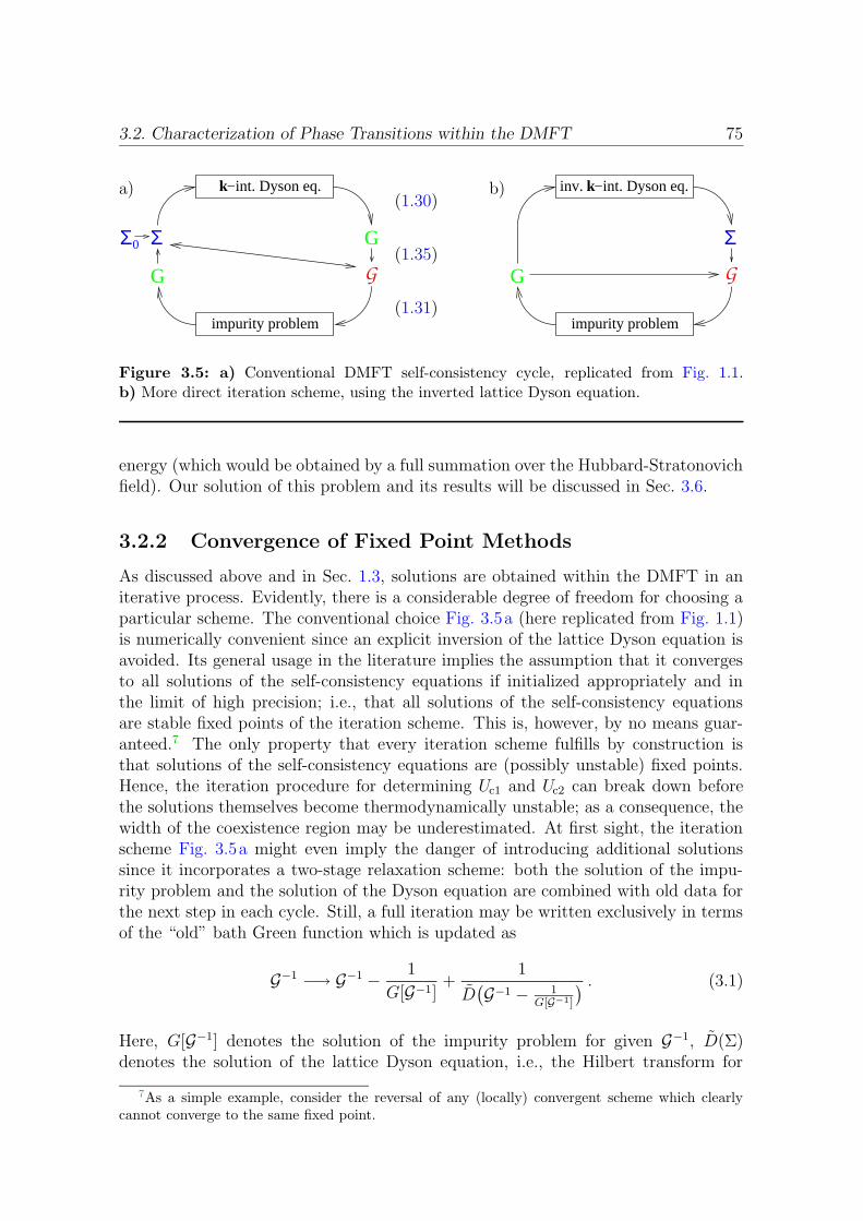
3.2. Characterization of Phase Transitions within the DMFT 75
−int. Dyson eq.k
Σ
G
G
impurity problem
G
Σ0
(1.30)
(1.35)
(1.31)
a) b) −int. Dyson eq.k
impurity problem
GG
Σ
inv.
Figure 3.5: a) Conventional DMFT self-consistency cycle, replicated from Fig. 1.1.b) More direct iteration scheme, using the inverted lattice Dyson equation.
energy (which would be obtained by a full summation over the Hubbard-Stratonovichfield). Our solution of this problem and its results will be discussed in Sec. 3.6.
3.2.2 Convergence of Fixed Point Methods
As discussed above and in Sec. 1.3, solutions are obtained within the DMFT in aniterative process. Evidently, there is a considerable degree of freedom for choosing aparticular scheme. The conventional choice Fig. 3.5a (here replicated from Fig. 1.1)is numerically convenient since an explicit inversion of the lattice Dyson equation isavoided. Its general usage in the literature implies the assumption that it convergesto all solutions of the self-consistency equations if initialized appropriately and inthe limit of high precision; i.e., that all solutions of the self-consistency equationsare stable fixed points of the iteration scheme. This is, however, by no means guar-anteed.7 The only property that every iteration scheme fulfills by construction isthat solutions of the self-consistency equations are (possibly unstable) fixed points.Hence, the iteration procedure for determining Uc1 and Uc2 can break down beforethe solutions themselves become thermodynamically unstable; as a consequence, thewidth of the coexistence region may be underestimated. At first sight, the iterationscheme Fig. 3.5a might even imply the danger of introducing additional solutionssince it incorporates a two-stage relaxation scheme: both the solution of the impu-rity problem and the solution of the Dyson equation are combined with old data forthe next step in each cycle. Still, a full iteration may be written exclusively in termsof the “old” bath Green function which is updated as
G−1 −→ G−1 − 1
G[G−1]+
1
D(G−1 − 1
G[G−1]
) . (3.1)
Here, G[G−1] denotes the solution of the impurity problem for given G−1, D(Σ)denotes the solution of the lattice Dyson equation, i.e., the Hilbert transform for
7As a simple example, consider the reversal of any (locally) convergent scheme which clearlycannot converge to the same fixed point.
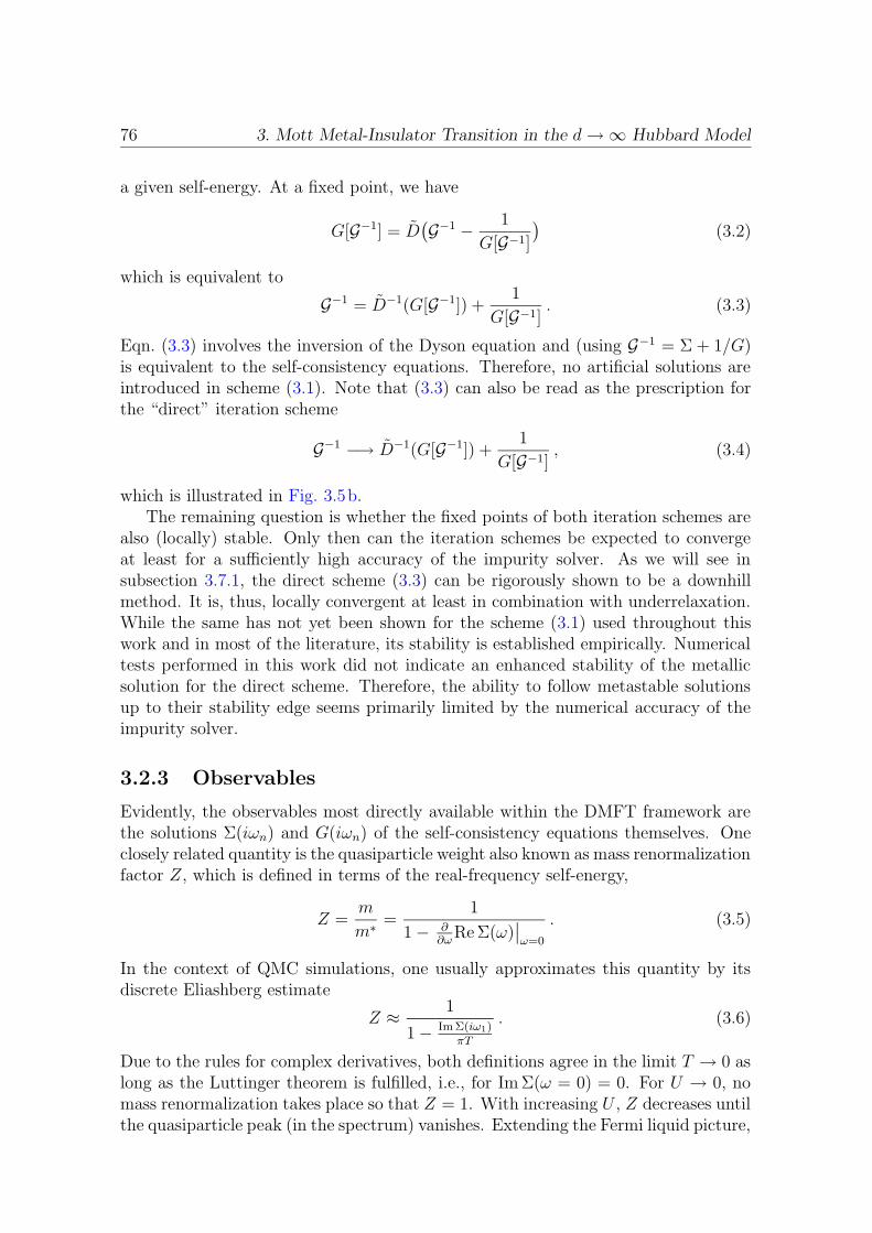
76 3. Mott Metal-Insulator Transition in the d→∞ Hubbard Model
a given self-energy. At a fixed point, we have
G[G−1] = D(G−1 − 1
G[G−1]
)(3.2)
which is equivalent to
G−1 = D−1(G[G−1]) +1
G[G−1]. (3.3)
Eqn. (3.3) involves the inversion of the Dyson equation and (using G−1 = Σ + 1/G)is equivalent to the self-consistency equations. Therefore, no artificial solutions areintroduced in scheme (3.1). Note that (3.3) can also be read as the prescription forthe “direct” iteration scheme
G−1 −→ D−1(G[G−1]) +1
G[G−1], (3.4)
which is illustrated in Fig. 3.5b.The remaining question is whether the fixed points of both iteration schemes are
also (locally) stable. Only then can the iteration schemes be expected to convergeat least for a sufficiently high accuracy of the impurity solver. As we will see insubsection 3.7.1, the direct scheme (3.3) can be rigorously shown to be a downhillmethod. It is, thus, locally convergent at least in combination with underrelaxation.While the same has not yet been shown for the scheme (3.1) used throughout thiswork and in most of the literature, its stability is established empirically. Numericaltests performed in this work did not indicate an enhanced stability of the metallicsolution for the direct scheme. Therefore, the ability to follow metastable solutionsup to their stability edge seems primarily limited by the numerical accuracy of theimpurity solver.
3.2.3 Observables
Evidently, the observables most directly available within the DMFT framework arethe solutions Σ(iωn) and G(iωn) of the self-consistency equations themselves. Oneclosely related quantity is the quasiparticle weight also known as mass renormalizationfactor Z, which is defined in terms of the real-frequency self-energy,
Z =m
m∗ =1
1− ∂∂ω
Re Σ(ω)∣∣ω=0
. (3.5)
In the context of QMC simulations, one usually approximates this quantity by itsdiscrete Eliashberg estimate
Z ≈ 1
1− Im Σ(iω1)πT
. (3.6)
Due to the rules for complex derivatives, both definitions agree in the limit T → 0 aslong as the Luttinger theorem is fulfilled, i.e., for Im Σ(ω = 0) = 0. For U → 0, nomass renormalization takes place so that Z = 1. With increasing U , Z decreases untilthe quasiparticle peak (in the spectrum) vanishes. Extending the Fermi liquid picture,
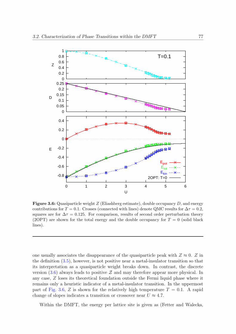
3.2. Characterization of Phase Transitions within the DMFT 77
-0.8
-0.6
-0.4
-0.2
0
0.2
0.4
0 1 2 3 4 5 6
E
U
EpotEtotEkin
2OPT: T=0
0
0.050.1
0.150.2
0.25
D
0
0.2
0.40.6
0.8
1
Z
T=0.1
Figure 3.6: Quasiparticle weight Z (Eliashberg estimate), double occupancyD, and energycontributions for T = 0.1. Crosses (connected with lines) denote QMC results for ∆τ = 0.2,squares are for ∆τ = 0.125. For comparison, results of second order perturbation theory(2OPT) are shown for the total energy and the double occupancy for T = 0 (solid blacklines).
one usually associates the disappearance of the quasiparticle peak with Z ≈ 0. Z inthe definition (3.5), however, is not positive near a metal-insulator transition so thatits interpretation as a quasiparticle weight breaks down. In contrast, the discreteversion (3.6) always leads to positive Z and may therefore appear more physical. Inany case, Z loses its theoretical foundation outside the Fermi liquid phase where itremains only a heuristic indicator of a metal-insulator transition. In the uppermostpart of Fig. 3.6, Z is shown for the relatively high temperature T = 0.1. A rapidchange of slopes indicates a transition or crossover near U ≈ 4.7.
Within the DMFT, the energy per lattice site is given as (Fetter and Walecka,
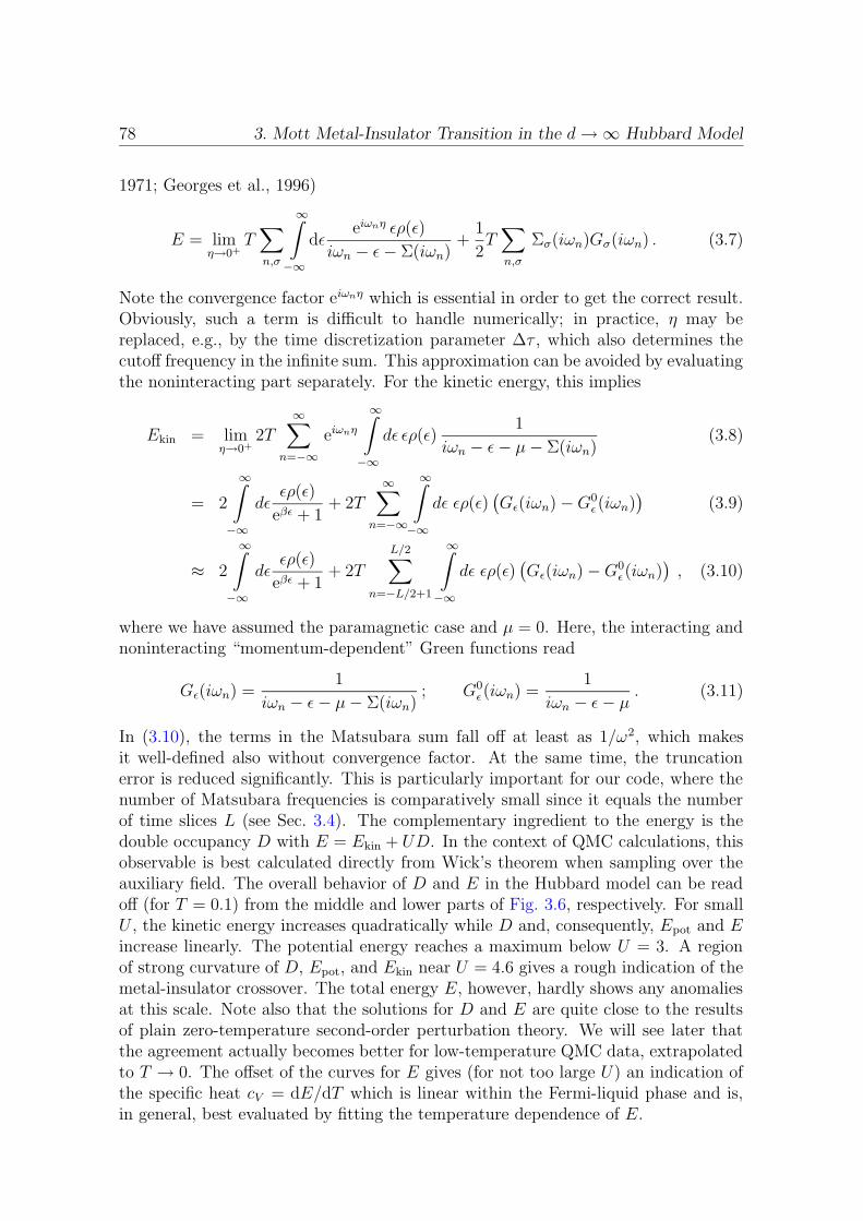
78 3. Mott Metal-Insulator Transition in the d→∞ Hubbard Model
1971; Georges et al., 1996)
E = limη→0+
T∑
n,σ
∞∫
−∞
dεeiωnη ερ(ε)
iωn − ε− Σ(iωn)+
1
2T∑
n,σ
Σσ(iωn)Gσ(iωn) . (3.7)
Note the convergence factor eiωnη which is essential in order to get the correct result.Obviously, such a term is difficult to handle numerically; in practice, η may bereplaced, e.g., by the time discretization parameter ∆τ , which also determines thecutoff frequency in the infinite sum. This approximation can be avoided by evaluatingthe noninteracting part separately. For the kinetic energy, this implies
Ekin = limη→0+
2T∞∑
n=−∞eiωnη
∞∫
−∞
dε ερ(ε)1
iωn − ε− µ− Σ(iωn)(3.8)
= 2
∞∫
−∞
dεερ(ε)
eβε + 1+ 2T
∞∑
n=−∞
∞∫
−∞
dε ερ(ε)(Gε(iωn)−G0
ε(iωn))
(3.9)
≈ 2
∞∫
−∞
dεερ(ε)
eβε + 1+ 2T
L/2∑
n=−L/2+1
∞∫
−∞
dε ερ(ε)(Gε(iωn)−G0
ε(iωn)), (3.10)
where we have assumed the paramagnetic case and µ = 0. Here, the interacting andnoninteracting “momentum-dependent” Green functions read
Gε(iωn) =1
iωn − ε− µ− Σ(iωn); G0
ε(iωn) =1
iωn − ε− µ. (3.11)
In (3.10), the terms in the Matsubara sum fall off at least as 1/ω2, which makesit well-defined also without convergence factor. At the same time, the truncationerror is reduced significantly. This is particularly important for our code, where thenumber of Matsubara frequencies is comparatively small since it equals the numberof time slices L (see Sec. 3.4). The complementary ingredient to the energy is thedouble occupancy D with E = Ekin + UD. In the context of QMC calculations, thisobservable is best calculated directly from Wick’s theorem when sampling over theauxiliary field. The overall behavior of D and E in the Hubbard model can be readoff (for T = 0.1) from the middle and lower parts of Fig. 3.6, respectively. For smallU , the kinetic energy increases quadratically while D and, consequently, Epot and Eincrease linearly. The potential energy reaches a maximum below U = 3. A regionof strong curvature of D, Epot, and Ekin near U = 4.6 gives a rough indication of themetal-insulator crossover. The total energy E, however, hardly shows any anomaliesat this scale. Note also that the solutions for D and E are quite close to the resultsof plain zero-temperature second-order perturbation theory. We will see later thatthe agreement actually becomes better for low-temperature QMC data, extrapolatedto T → 0. The offset of the curves for E gives (for not too large U) an indication ofthe specific heat cV = dE/dT which is linear within the Fermi-liquid phase and is,in general, best evaluated by fitting the temperature dependence of E.
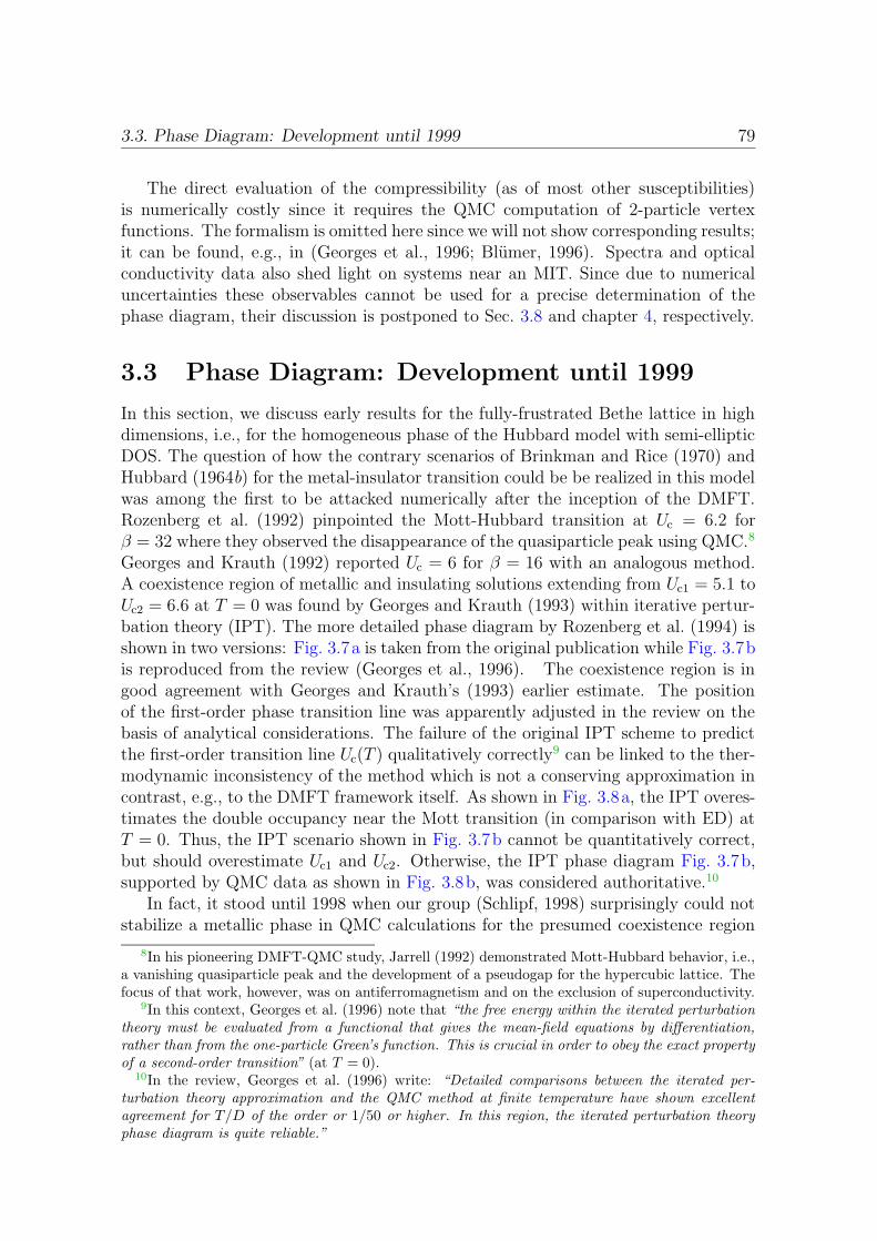
3.3. Phase Diagram: Development until 1999 79
The direct evaluation of the compressibility (as of most other susceptibilities)is numerically costly since it requires the QMC computation of 2-particle vertexfunctions. The formalism is omitted here since we will not show corresponding results;it can be found, e.g., in (Georges et al., 1996; Blumer, 1996). Spectra and opticalconductivity data also shed light on systems near an MIT. Since due to numericaluncertainties these observables cannot be used for a precise determination of thephase diagram, their discussion is postponed to Sec. 3.8 and chapter 4, respectively.
3.3 Phase Diagram: Development until 1999
In this section, we discuss early results for the fully-frustrated Bethe lattice in highdimensions, i.e., for the homogeneous phase of the Hubbard model with semi-ellipticDOS. The question of how the contrary scenarios of Brinkman and Rice (1970) andHubbard (1964b) for the metal-insulator transition could be be realized in this modelwas among the first to be attacked numerically after the inception of the DMFT.Rozenberg et al. (1992) pinpointed the Mott-Hubbard transition at Uc = 6.2 forβ = 32 where they observed the disappearance of the quasiparticle peak using QMC.8
Georges and Krauth (1992) reported Uc = 6 for β = 16 with an analogous method.A coexistence region of metallic and insulating solutions extending from Uc1 = 5.1 toUc2 = 6.6 at T = 0 was found by Georges and Krauth (1993) within iterative pertur-bation theory (IPT). The more detailed phase diagram by Rozenberg et al. (1994) isshown in two versions: Fig. 3.7a is taken from the original publication while Fig. 3.7bis reproduced from the review (Georges et al., 1996). The coexistence region is ingood agreement with Georges and Krauth’s (1993) earlier estimate. The positionof the first-order phase transition line was apparently adjusted in the review on thebasis of analytical considerations. The failure of the original IPT scheme to predictthe first-order transition line Uc(T ) qualitatively correctly9 can be linked to the ther-modynamic inconsistency of the method which is not a conserving approximation incontrast, e.g., to the DMFT framework itself. As shown in Fig. 3.8a, the IPT overes-timates the double occupancy near the Mott transition (in comparison with ED) atT = 0. Thus, the IPT scenario shown in Fig. 3.7b cannot be quantitatively correct,but should overestimate Uc1 and Uc2. Otherwise, the IPT phase diagram Fig. 3.7b,supported by QMC data as shown in Fig. 3.8b, was considered authoritative.10
In fact, it stood until 1998 when our group (Schlipf, 1998) surprisingly could notstabilize a metallic phase in QMC calculations for the presumed coexistence region
8In his pioneering DMFT-QMC study, Jarrell (1992) demonstrated Mott-Hubbard behavior, i.e.,a vanishing quasiparticle peak and the development of a pseudogap for the hypercubic lattice. Thefocus of that work, however, was on antiferromagnetism and on the exclusion of superconductivity.
9In this context, Georges et al. (1996) note that “the free energy within the iterated perturbationtheory must be evaluated from a functional that gives the mean-field equations by differentiation,rather than from the one-particle Green’s function. This is crucial in order to obey the exact propertyof a second-order transition” (at T = 0).
10In the review, Georges et al. (1996) write: “Detailed comparisons between the iterated per-turbation theory approximation and the QMC method at finite temperature have shown excellentagreement for T/D of the order or 1/50 or higher. In this region, the iterated perturbation theoryphase diagram is quite reliable.”
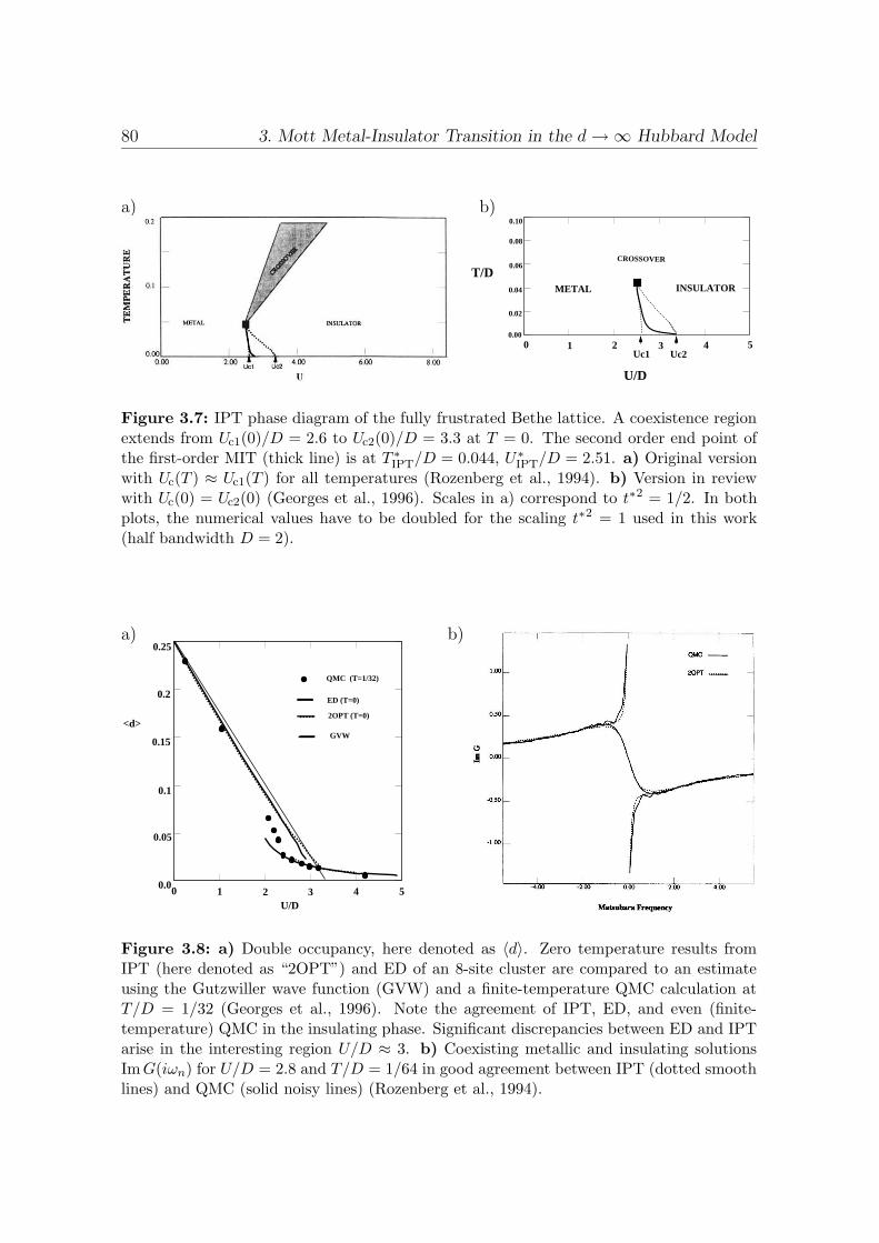
80 3. Mott Metal-Insulator Transition in the d→∞ Hubbard Model
a) b)
U/D
METAL INSULATOR
CROSSOVER
Uc1 Uc2
T/D
0 1 2 3 4 5
0.10
0.08
0.06
0.04
0.02
0.00
Figure 3.7: IPT phase diagram of the fully frustrated Bethe lattice. A coexistence regionextends from Uc1(0)/D = 2.6 to Uc2(0)/D = 3.3 at T = 0. The second order end point ofthe first-order MIT (thick line) is at T ∗
IPT/D = 0.044, U∗IPT/D = 2.51. a) Original version
with Uc(T ) ≈ Uc1(T ) for all temperatures (Rozenberg et al., 1994). b) Version in reviewwith Uc(0) = Uc2(0) (Georges et al., 1996). Scales in a) correspond to t∗2 = 1/2. In bothplots, the numerical values have to be doubled for the scaling t∗2 = 1 used in this work(half bandwidth D = 2).
a) b)0.25
QMC (T=1/32)
2OPT (T=0)
0.2
0.15
0.1
0.05
0.00 1 2 3 4 5
U/D
ED (T=0)
<d>GVW
Figure 3.8: a) Double occupancy, here denoted as 〈d〉. Zero temperature results fromIPT (here denoted as “2OPT”) and ED of an 8-site cluster are compared to an estimateusing the Gutzwiller wave function (GVW) and a finite-temperature QMC calculation atT/D = 1/32 (Georges et al., 1996). Note the agreement of IPT, ED, and even (finite-temperature) QMC in the insulating phase. Significant discrepancies between ED and IPTarise in the interesting region U/D ≈ 3. b) Coexisting metallic and insulating solutionsImG(iωn) for U/D = 2.8 and T/D = 1/64 in good agreement between IPT (dotted smoothlines) and QMC (solid noisy lines) (Rozenberg et al., 1994).
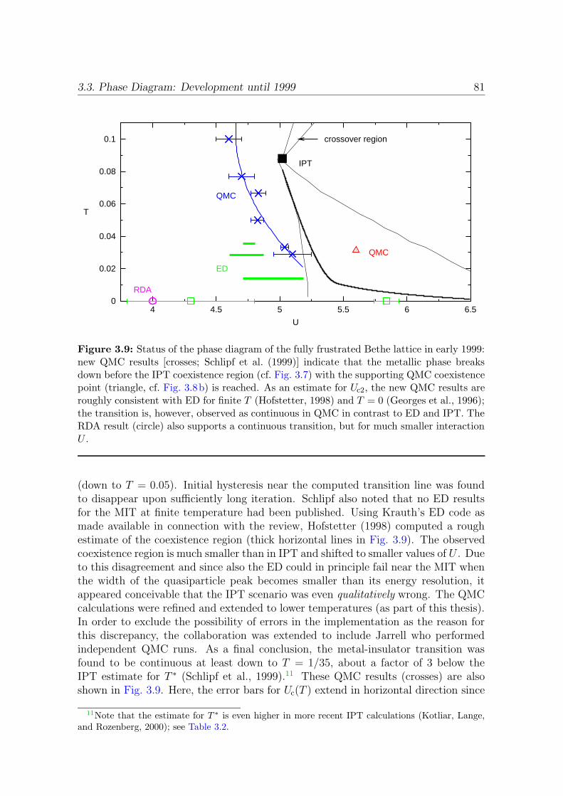
3.3. Phase Diagram: Development until 1999 81
0
0.02
0.04
0.06
0.08
0.1
4 4.5 5 5.5 6 6.5
T
U
crossover region
IPT
QMC
ED
RDA
QMC
Figure 3.9: Status of the phase diagram of the fully frustrated Bethe lattice in early 1999:new QMC results [crosses; Schlipf et al. (1999)] indicate that the metallic phase breaksdown before the IPT coexistence region (cf. Fig. 3.7) with the supporting QMC coexistencepoint (triangle, cf. Fig. 3.8b) is reached. As an estimate for Uc2, the new QMC results areroughly consistent with ED for finite T (Hofstetter, 1998) and T = 0 (Georges et al., 1996);the transition is, however, observed as continuous in QMC in contrast to ED and IPT. TheRDA result (circle) also supports a continuous transition, but for much smaller interactionU .
(down to T = 0.05). Initial hysteresis near the computed transition line was foundto disappear upon sufficiently long iteration. Schlipf also noted that no ED resultsfor the MIT at finite temperature had been published. Using Krauth’s ED code asmade available in connection with the review, Hofstetter (1998) computed a roughestimate of the coexistence region (thick horizontal lines in Fig. 3.9). The observedcoexistence region is much smaller than in IPT and shifted to smaller values of U . Dueto this disagreement and since also the ED could in principle fail near the MIT whenthe width of the quasiparticle peak becomes smaller than its energy resolution, itappeared conceivable that the IPT scenario was even qualitatively wrong. The QMCcalculations were refined and extended to lower temperatures (as part of this thesis).In order to exclude the possibility of errors in the implementation as the reason forthis discrepancy, the collaboration was extended to include Jarrell who performedindependent QMC runs. As a final conclusion, the metal-insulator transition wasfound to be continuous at least down to T = 1/35, about a factor of 3 below theIPT estimate for T ∗ (Schlipf et al., 1999).11 These QMC results (crosses) are alsoshown in Fig. 3.9. Here, the error bars for Uc(T ) extend in horizontal direction since
11Note that the estimate for T ∗ is even higher in more recent IPT calculations (Kotliar, Lange,and Rozenberg, 2000); see Table 3.2.

82 3. Mott Metal-Insulator Transition in the d→∞ Hubbard Model
the QMC hysteresis runs were performed at constant temperature. The interpolatingline is a guide to the eye only; it is certainly compatible with the T = 0 estimates forUc2 by ED and PSCT (Moeller, Si, Kotliar, Rozenberg, and Fisher, 1995). Still, thescenario of a continuous transition is in fundamental qualitative disagreement withboth ED (squares in Fig. 3.9 indicate the zero-temperature results, note the largeerror bars) and IPT.
Our controversial result stirred new interest in the problem. Qualitatively, thecontinuous scenario was supported by results from the random-dispersion approxi-mation (RDA), evaluated using ED on a small cluster. Quantitatively, however, theagreement was hardly better than, e.g., with IPT, since the (zero-temperature) RDAresult of Uc = 4 (shown as a circle in Fig. 3.9) is clearly too small to be compatiblewith the QMC data.
The result of a new QMC study by Rozenberg, Chitra, and Kotliar (1999), incontrast, was quantitatively almost compatible with our data (within double errorbars12). It also confirmed that the QMC coexistence point computed earlier by Rozen-berg et al. (1994) and shown as triangle in Fig. 3.9 was indeed incorrect. However,the new study demonstrated the coexistence of metallic and insulating solutions (tri-angles in Fig. 3.10) in a temperature range where Schlipf et al. (1999) had ruled out afirst-order transition. Further support for the scenario of a first order transition camefrom zero-temperature NRG studies (Bulla, 1999). The resolution of this contradic-tion, obtained for the same model (and now even using the same numerical methods)became an important project for this thesis and will be the subject of the remainderof this chapter. The first part, the verification of coexistence, was accomplished inthe fall of 1999, soon after Rozenberg made available a set of QMC estimates forG(τ) and G(τ) in both the metallic and insulating phase for the single parameter setT = 1/32, U = 4.92 (cf. Fig. 3.12).13 At this point, all involved groups accepted thata finite, but small coexistence region was established in the lowest temperature rangestudied so far using QMC. Still, the shapes of the coexistence region were unclear.The thick solid lines in Fig. 3.10 represent Kotliar’s perception that the region shouldbroaden significantly for lower T , reaching the RDA point for Uc1 and matching the(practically identical) estimates for Uc2 obtained using ED, PSCT, and NRG (seeTable 3.1 on page 112).
3.4 Discussion of QMC Algorithms
In the main part of this section, we will discuss two aspects of the quantum MonteCarlo (QMC) algorithm for the DMFT self-consistency problem: the discrete Fouriertransformations between imaginary time and Matsubara frequencies and the searchstrategy for solutions of the DMFT equations. Both aspects are directly relevantfor the detection of the Mott transition and the associated coexistence region. Thedifferent algorithms for handling the discrete Fourier transform used in the codes
12The point at T = 1/30 with the small error bar was not computed as part of this thesis.13Note that this phase point is not among the previously published data, but more in the center
of the claimed coexistence region.
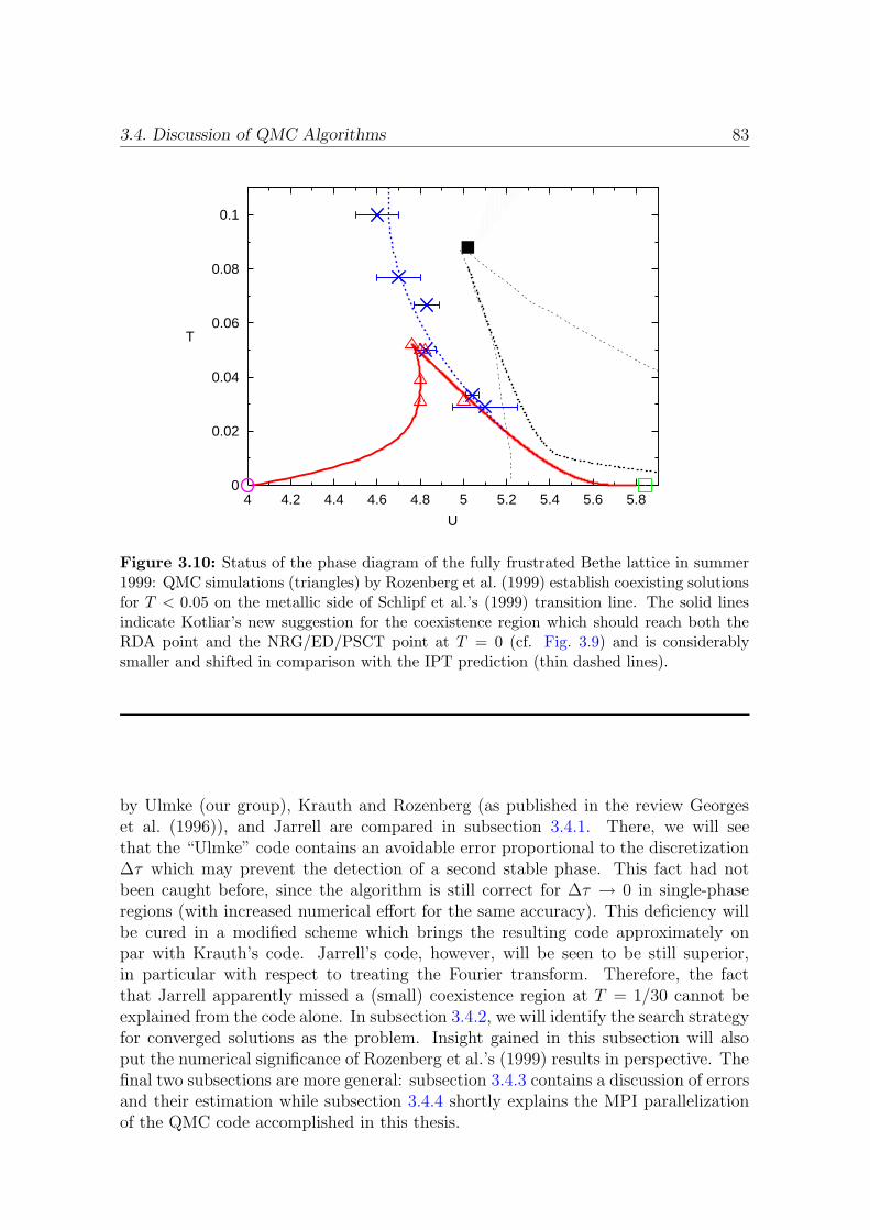
3.4. Discussion of QMC Algorithms 83
0
0.02
0.04
0.06
0.08
0.1
4 4.2 4.4 4.6 4.8 5 5.2 5.4 5.6 5.8
T
U
Figure 3.10: Status of the phase diagram of the fully frustrated Bethe lattice in summer1999: QMC simulations (triangles) by Rozenberg et al. (1999) establish coexisting solutionsfor T < 0.05 on the metallic side of Schlipf et al.’s (1999) transition line. The solid linesindicate Kotliar’s new suggestion for the coexistence region which should reach both theRDA point and the NRG/ED/PSCT point at T = 0 (cf. Fig. 3.9) and is considerablysmaller and shifted in comparison with the IPT prediction (thin dashed lines).
by Ulmke (our group), Krauth and Rozenberg (as published in the review Georgeset al. (1996)), and Jarrell are compared in subsection 3.4.1. There, we will seethat the “Ulmke” code contains an avoidable error proportional to the discretization∆τ which may prevent the detection of a second stable phase. This fact had notbeen caught before, since the algorithm is still correct for ∆τ → 0 in single-phaseregions (with increased numerical effort for the same accuracy). This deficiency willbe cured in a modified scheme which brings the resulting code approximately onpar with Krauth’s code. Jarrell’s code, however, will be seen to be still superior,in particular with respect to treating the Fourier transform. Therefore, the factthat Jarrell apparently missed a (small) coexistence region at T = 1/30 cannot beexplained from the code alone. In subsection 3.4.2, we will identify the search strategyfor converged solutions as the problem. Insight gained in this subsection will alsoput the numerical significance of Rozenberg et al.’s (1999) results in perspective. Thefinal two subsections are more general: subsection 3.4.3 contains a discussion of errorsand their estimation while subsection 3.4.4 shortly explains the MPI parallelizationof the QMC code accomplished in this thesis.
84 3. Mott Metal-Insulator Transition in the d→∞ Hubbard Model
3.4.1 Fourier Transformation and Smoothing
A QMC simulation within the DMFT framework consists of a simultaneous solutionof two principal equations: the lattice Dyson equation (1.30) and the defining ex-pression for the impurity Green function (1.31). The IPT and QMC solutions of theimpurity problem are formulated in imaginary time, i.e., the bath Green functionG is needed as function of τ and the result is expressed as G(τ). In contrast, theDyson equation is formulated (and is local) in the frequency domain, here for Mat-subara frequencies iωn = i(2n+ 1)πT . Therefore, two Fourier transformations (fromfrequency to imaginary time and vice versa) per self-consistency cycle are necessary,which for G read
G(iωn) =
β∫
0
dτ eiωnτ G(τ) (3.12)
G(τ) =1
β
∞∑
n=−∞e−iωnτ G(iωn) . (3.13)
Note that (3.13) implies antiperiodicity of G(τ) for translations β (since eiωnβ = −1)and allows for a discontinuity of G(τ) (at τ = 0) since the number of terms is infinite.The spectral representation of G implies a decay of G(iωn) as 1/iωn for |n| → ∞ likefor any normalized analytic function. Furthermore, G(iωn) is purely imaginary whenG(τ) = G(β − τ) as in the case of interest.
Discretization Problem
Numerically, however, the integral in (3.12) needs to be discretized and the Matsubarasum in (3.13) has to be truncated. Since the numerical effort in QMC scales with thenumber Λ = β/∆τ of discretized time slices at least14 as Λ3, this method is presentlyrestricted to Λ . 400. Typically, 200 time slices and less are used. A naive discreteversion of the Fourier transform,
G(iωn) = ∆τ(G(0)−G(β)
2+
Λ−1∑
l=1
eiωnτl G(τl))
; τl := l∆τ (3.14)
G(τl) =1
β
Λ/2−1∑
n=−Λ/2
e−iωnτl G(iωn) , (3.15)
fails for such a coarse grid. The problems are that the Green function G(τ) estimatedfrom a finite Matsubara sum can not be discontinuous at τ = 0 (as required analyti-cally for G(τ)) while the discrete estimate G(iωn) oscillates with periodicity 2πiΛ/βinstead of decaying for large frequencies. This implies a large error of G(iωn) when|ωn| approaches or exceeds the Nyquist frequency πΛ/β. Both (related) effects would
14In practice, the scaling is even worse on systems with a hierarchy of memory systems of increasingcapacity and decreasing speed.

3.4. Discussion of QMC Algorithms 85
make the evaluation of the corresponding self-consistency equations pointless. Inparticular, in the naive scheme, the self-energy diverges near the Nyquist frequency.Finally, the sum in (3.15) is numerically somewhat unstable since G(τ) also oscillatesbetween the grid points τl.
Splining Method
Fortunately, there is physical information left that has not been used in the naivescheme: G(τ) is known to be a smooth function. In fact, it follows from (1.55) and(1.56) that G(τ) and all even derivatives are positive definite and, consequently, reachtheir maxima at the edges τ = 0 and τ = β. This knowledge of “smoothness” can beexploited in a spline interpolation of the QMC result G(τl)Λl=0 by piecewise cubicpolynomials. The resulting functions may then either be used for oversampling, i.e.,for generating G(τ) on a finite grid or for piecewise direct analytic Fourier transforms.In both cases, G(iωn) can be calculated for a much larger frequency range than be-fore. Jarrell, Akhlaghpour, and Pruschke (1993) used oversampling with typically800 Matsubara frequencies. The second choice mentioned above is implemented inKrauth’s program: for any choice of Λ, G(iωn) is evaluated for a very large number(by default N = 213 = 8192) of Matsubara frequencies. While the spline interpo-lation incorporates some physical information, it is clearly not exact; therefore, themethod used on its own has its limits. Jarrell noted that the usual cubic splineswith continuous second derivative were dangerous in this respect since they tend togenerate artificial high-frequency features. This effect was found to be reduced usingAkima splines. Both implementations use splines with natural boundary conditions,i.e., with vanishing second derivative at the end points.
As we noted recently, this is in general not a good choice; after all, the true secondderivatives are maximal at the end points. The bad fit at the boundaries then leadsto ringing (which decays faster for Akima splines). An implementation with freeboundary conditions for the second derivative which are determined in an iterativeminimalization scheme was found to be vastly superior over both schemes at leastfor a restricted set of test cases. The minimization procedure can even be avoidedby computing the second derivative of G(τ) at τ = 0 exactly. A related method forimproving on the natural spline scheme is to interpolate not G(τl)Λl=0, but only thedifference with respect to some reference Green function obtained from, e.g., plainsecond order perturbation theory or IPT. This approach, discussed in a general con-text by Deisz, Hess, and Serene (1995), is implemented in Jarrell’s code. In addition,the high-frequency part may be directly stabilized by supplementing the QMC es-timates with IPT (using low-pass/high-pass filters). Since each of the approachesdiscussed so far generates a number of Matsubara frequencies which is much greaterthan the number of time slices, the inverse Fourier transform is unproblematic: therounding-off near τ = 0 is already small for the first grid point τ = ∆τ while at theend points τ = 0 and τ = β, the numerical Fourier transforms can be shifted bythe value 1/2 to exactly cancel the rounding effect. For more information on recentdevelopments, see App. C and Knecht’s (2002) diploma thesis.

86 3. Mott Metal-Insulator Transition in the d→∞ Hubbard Model
Ulmke’s Smoothing Trick
A completely different approach was taken by Ulmke (1995). Here, the numberof Matsubara frequencies is chosen equal to the number of time slices. In order toenforce the correct analytical behavior of the Fourier transforms, a “smoothing” trickis employed: the naive Fourier transform is combined with an approximate correctingtransformation which approaches the identity for ∆τ → 0. The algorithm consists ofthe following two steps:
1. Asymmetric naive Fourier transform G(iωn) = ∆τ∑Λ−1
l=0 eiωnτl G(τl). The dif-ference to the symmetric transform (3.14) is a constant finite real term ∆τ/2.
2. Smoothing transformation
G(iωn) =∆τ
ln(1 + ∆τ/G(iωn)). (3.16)
This corrected Green function fulfills ReG(ω) = 0 (for half filling and symmetricDOS) and (approximately) G(iωn) ∝ 1/(iωn) for ω → ±ωmax. By using the inversecorrection transform G(ω) = ∆τ/(exp(∆τ/G(ω) − 1)) before the inverse Fouriertransform, also the artifacts in G(τ) (or G(τ)) are removed. Ulmke’s (1995) claimthat the transformation scheme would be exact in the noninteracting and in theatomic limit is, however, incorrect. The assumed asymptotic form G(iωn) = 1/(iωn)for hopping t = 0 applies only to the degenerate U = 0 case. Otherwise, G(iωn)is linear for small frequencies in the insulating regime. This misconception alreadypoints towards the main deficiency of the scheme: in order to cure a problem at highfrequencies, a transformation is applied which changes G irrespective of the frequency.In fact, all values of G are modified significantly which are not large compared to∆τ . Among this group, however, are not only points near the Nyquist frequency, butalso those with small iωn (in the insulator). Consequently, Ulmke’s approach treatsinsulating solutions much worse than metallic solutions.
In order to illustrate this effect and for a general quantitative comparison, weused the insulating solution G(τ) for β = 32, U = 4.92, and ∆τ = 0.25 as providedby Rozenberg as input for the various Fourier transformation schemes. Each outputG(iωn) was then transformed to the corresponding self-energy Σ(iωn) via the invertedBethe lattice Dyson equation. As shown in Fig. 3.11, only Jarrell’s algorithm yieldsa self-energy with the correct analytic form, i.e., with negative imaginary part for allpositive ωn.
15 While Ulmke’s algorithm just stops at the Nyquist frequency π/∆τ ,Krauth’s code overshoots substantially (see also right inset).16 At small frequencies,the results of Krauth’s method and of Jarrell’s method agree very well (left inset),
15Slight deviations from the quantitatively correct asymptotic form for very large frequencies (notshown) could have been avoided by using the exact asymptotic expression Σ(iωn) → U2/(4iωn) inthis regime; cf. App. C.
16This overshooting can be attributed to the use of natural splines; it might have been overlookedsince the original code does not output frequency information. The origin of slight deviationsfor intermediate frequencies ωn ≈ 1 (in comparison with the curves for Jarrell’s method and themodified Ulmke method) is unclear.
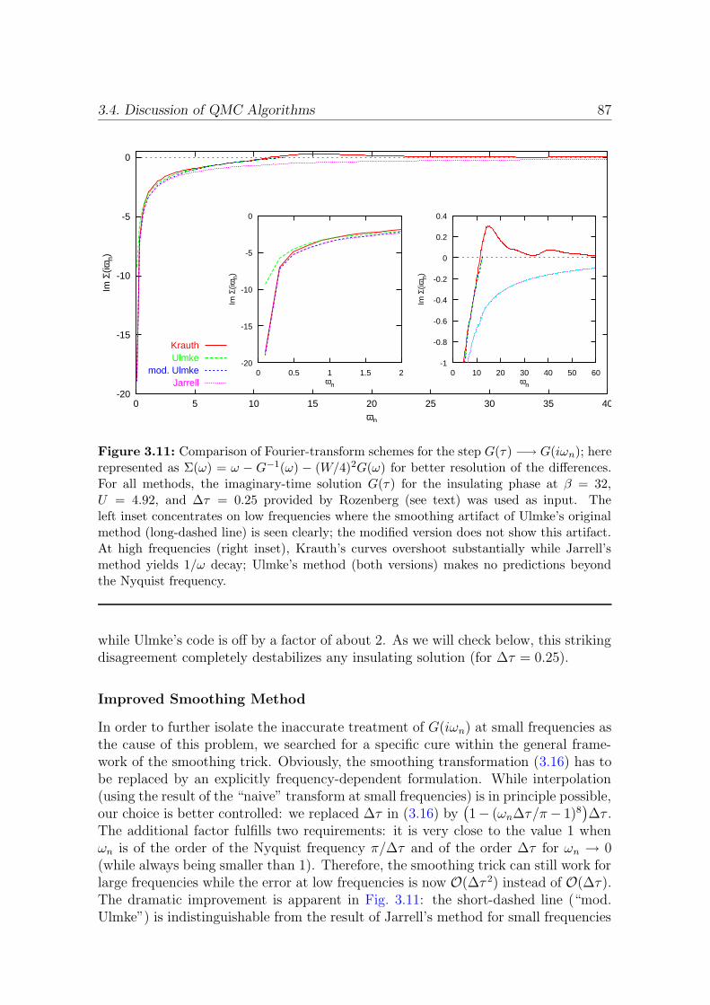
3.4. Discussion of QMC Algorithms 87
-20
-15
-10
-5
0
0 5 10 15 20 25 30 35 40
Im Σ
(iωn)
ωn
KrauthUlmke
mod. UlmkeJarrell
-20
-15
-10
-5
0
0 0.5 1 1.5 2
Im Σ
(iωn)
ωn
-1
-0.8
-0.6
-0.4
-0.2
0
0.2
0.4
0 10 20 30 40 50 60
Im Σ
(iωn)
ωn
Figure 3.11: Comparison of Fourier-transform schemes for the step G(τ) −→ G(iωn); hererepresented as Σ(ω) = ω − G−1(ω) − (W/4)2G(ω) for better resolution of the differences.For all methods, the imaginary-time solution G(τ) for the insulating phase at β = 32,U = 4.92, and ∆τ = 0.25 provided by Rozenberg (see text) was used as input. Theleft inset concentrates on low frequencies where the smoothing artifact of Ulmke’s originalmethod (long-dashed line) is seen clearly; the modified version does not show this artifact.At high frequencies (right inset), Krauth’s curves overshoot substantially while Jarrell’smethod yields 1/ω decay; Ulmke’s method (both versions) makes no predictions beyondthe Nyquist frequency.
while Ulmke’s code is off by a factor of about 2. As we will check below, this strikingdisagreement completely destabilizes any insulating solution (for ∆τ = 0.25).
Improved Smoothing Method
In order to further isolate the inaccurate treatment of G(iωn) at small frequencies asthe cause of this problem, we searched for a specific cure within the general frame-work of the smoothing trick. Obviously, the smoothing transformation (3.16) has tobe replaced by an explicitly frequency-dependent formulation. While interpolation(using the result of the “naive” transform at small frequencies) is in principle possible,our choice is better controlled: we replaced ∆τ in (3.16) by
(1− (ωn∆τ/π− 1)8
)∆τ .
The additional factor fulfills two requirements: it is very close to the value 1 whenωn is of the order of the Nyquist frequency π/∆τ and of the order ∆τ for ωn → 0(while always being smaller than 1). Therefore, the smoothing trick can still work forlarge frequencies while the error at low frequencies is now O(∆τ 2) instead of O(∆τ).The dramatic improvement is apparent in Fig. 3.11: the short-dashed line (“mod.Ulmke”) is indistinguishable from the result of Jarrell’s method for small frequencies
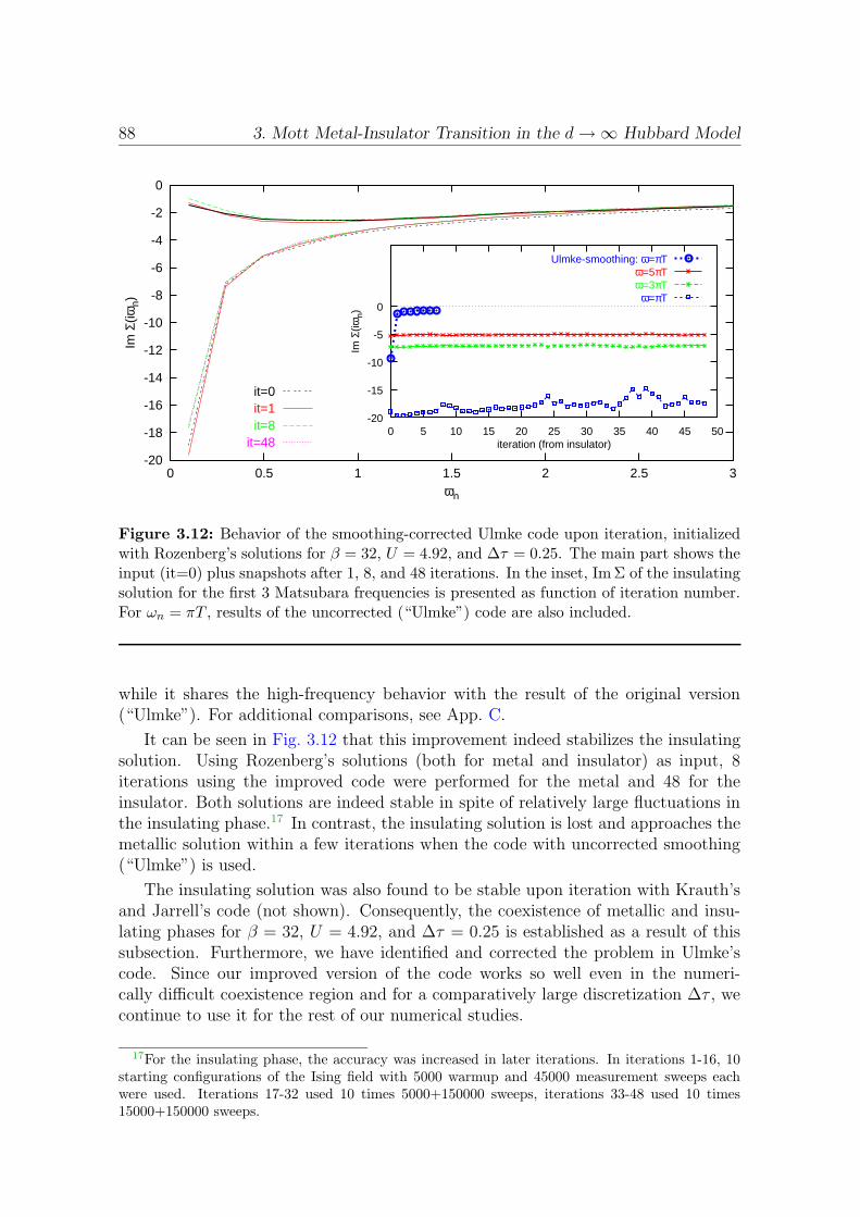
88 3. Mott Metal-Insulator Transition in the d→∞ Hubbard Model
-20
-18
-16
-14
-12
-10
-8
-6
-4
-2
0
0 0.5 1 1.5 2 2.5 3
Im Σ
(iωn)
ωn
it=0it=1it=8
it=48
-20
-15
-10
-5
0
0 5 10 15 20 25 30 35 40 45 50
Im Σ
(iωn)
iteration (from insulator)
Ulmke-smoothing: ω=πTω=5πTω=3πT
ω=πT
Figure 3.12: Behavior of the smoothing-corrected Ulmke code upon iteration, initializedwith Rozenberg’s solutions for β = 32, U = 4.92, and ∆τ = 0.25. The main part shows theinput (it=0) plus snapshots after 1, 8, and 48 iterations. In the inset, Im Σ of the insulatingsolution for the first 3 Matsubara frequencies is presented as function of iteration number.For ωn = πT , results of the uncorrected (“Ulmke”) code are also included.
while it shares the high-frequency behavior with the result of the original version(“Ulmke”). For additional comparisons, see App. C.
It can be seen in Fig. 3.12 that this improvement indeed stabilizes the insulatingsolution. Using Rozenberg’s solutions (both for metal and insulator) as input, 8iterations using the improved code were performed for the metal and 48 for theinsulator. Both solutions are indeed stable in spite of relatively large fluctuations inthe insulating phase.17 In contrast, the insulating solution is lost and approaches themetallic solution within a few iterations when the code with uncorrected smoothing(“Ulmke”) is used.
The insulating solution was also found to be stable upon iteration with Krauth’sand Jarrell’s code (not shown). Consequently, the coexistence of metallic and insu-lating phases for β = 32, U = 4.92, and ∆τ = 0.25 is established as a result of thissubsection. Furthermore, we have identified and corrected the problem in Ulmke’scode. Since our improved version of the code works so well even in the numeri-cally difficult coexistence region and for a comparatively large discretization ∆τ , wecontinue to use it for the rest of our numerical studies.
17For the insulating phase, the accuracy was increased in later iterations. In iterations 1-16, 10starting configurations of the Ising field with 5000 warmup and 45000 measurement sweeps eachwere used. Iterations 17-32 used 10 times 5000+150000 sweeps, iterations 33-48 used 10 times15000+150000 sweeps.
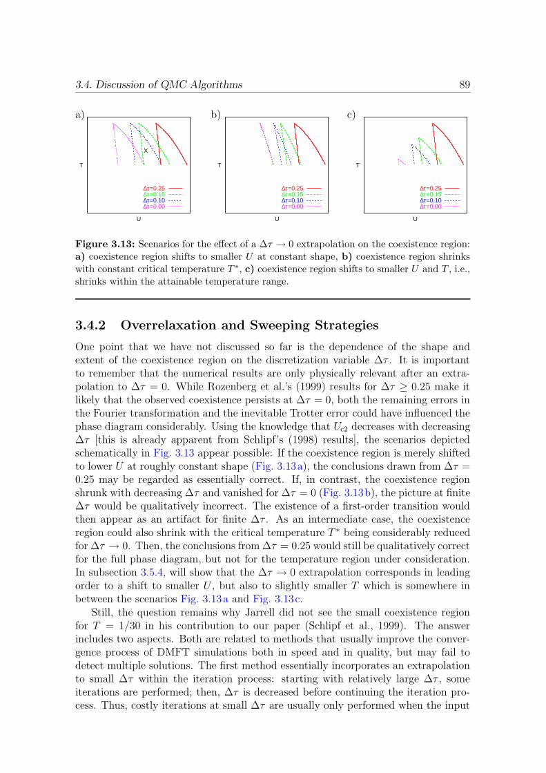
3.4. Discussion of QMC Algorithms 89
a) b) c)
T
U
X
∆τ=0.25∆τ=0.15∆τ=0.10∆τ=0.00
T
U
∆τ=0.25∆τ=0.15∆τ=0.10∆τ=0.00
T
U
∆τ=0.25∆τ=0.15∆τ=0.10∆τ=0.00
Figure 3.13: Scenarios for the effect of a ∆τ → 0 extrapolation on the coexistence region:a) coexistence region shifts to smaller U at constant shape, b) coexistence region shrinkswith constant critical temperature T ∗, c) coexistence region shifts to smaller U and T , i.e.,shrinks within the attainable temperature range.
3.4.2 Overrelaxation and Sweeping Strategies
One point that we have not discussed so far is the dependence of the shape andextent of the coexistence region on the discretization variable ∆τ . It is importantto remember that the numerical results are only physically relevant after an extra-polation to ∆τ = 0. While Rozenberg et al.’s (1999) results for ∆τ ≥ 0.25 make itlikely that the observed coexistence persists at ∆τ = 0, both the remaining errors inthe Fourier transformation and the inevitable Trotter error could have influenced thephase diagram considerably. Using the knowledge that Uc2 decreases with decreasing∆τ [this is already apparent from Schlipf’s (1998) results], the scenarios depictedschematically in Fig. 3.13 appear possible: If the coexistence region is merely shiftedto lower U at roughly constant shape (Fig. 3.13a), the conclusions drawn from ∆τ =0.25 may be regarded as essentially correct. If, in contrast, the coexistence regionshrunk with decreasing ∆τ and vanished for ∆τ = 0 (Fig. 3.13b), the picture at finite∆τ would be qualitatively incorrect. The existence of a first-order transition wouldthen appear as an artifact for finite ∆τ . As an intermediate case, the coexistenceregion could also shrink with the critical temperature T ∗ being considerably reducedfor ∆τ → 0. Then, the conclusions from ∆τ = 0.25 would still be qualitatively correctfor the full phase diagram, but not for the temperature region under consideration.In subsection 3.5.4, will show that the ∆τ → 0 extrapolation corresponds in leadingorder to a shift to smaller U , but also to slightly smaller T which is somewhere inbetween the scenarios Fig. 3.13a and Fig. 3.13c.
Still, the question remains why Jarrell did not see the small coexistence regionfor T = 1/30 in his contribution to our paper (Schlipf et al., 1999). The answerincludes two aspects. Both are related to methods that usually improve the conver-gence process of DMFT simulations both in speed and in quality, but may fail todetect multiple solutions. The first method essentially incorporates an extrapolationto small ∆τ within the iteration process: starting with relatively large ∆τ , someiterations are performed; then, ∆τ is decreased before continuing the iteration pro-cess. Thus, costly iterations at small ∆τ are usually only performed when the input
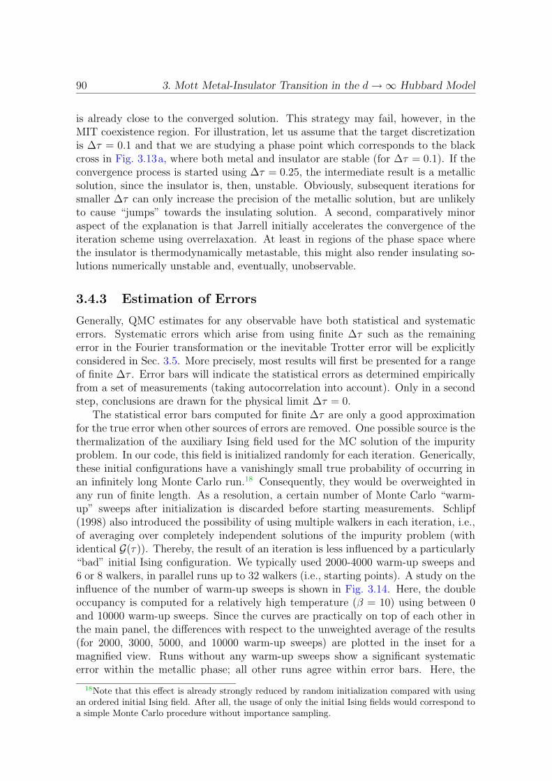
90 3. Mott Metal-Insulator Transition in the d→∞ Hubbard Model
is already close to the converged solution. This strategy may fail, however, in theMIT coexistence region. For illustration, let us assume that the target discretizationis ∆τ = 0.1 and that we are studying a phase point which corresponds to the blackcross in Fig. 3.13a, where both metal and insulator are stable (for ∆τ = 0.1). If theconvergence process is started using ∆τ = 0.25, the intermediate result is a metallicsolution, since the insulator is, then, unstable. Obviously, subsequent iterations forsmaller ∆τ can only increase the precision of the metallic solution, but are unlikelyto cause “jumps” towards the insulating solution. A second, comparatively minoraspect of the explanation is that Jarrell initially accelerates the convergence of theiteration scheme using overrelaxation. At least in regions of the phase space wherethe insulator is thermodynamically metastable, this might also render insulating so-lutions numerically unstable and, eventually, unobservable.
3.4.3 Estimation of Errors
Generally, QMC estimates for any observable have both statistical and systematicerrors. Systematic errors which arise from using finite ∆τ such as the remainingerror in the Fourier transformation or the inevitable Trotter error will be explicitlyconsidered in Sec. 3.5. More precisely, most results will first be presented for a rangeof finite ∆τ . Error bars will indicate the statistical errors as determined empiricallyfrom a set of measurements (taking autocorrelation into account). Only in a secondstep, conclusions are drawn for the physical limit ∆τ = 0.
The statistical error bars computed for finite ∆τ are only a good approximationfor the true error when other sources of errors are removed. One possible source is thethermalization of the auxiliary Ising field used for the MC solution of the impurityproblem. In our code, this field is initialized randomly for each iteration. Generically,these initial configurations have a vanishingly small true probability of occurring inan infinitely long Monte Carlo run.18 Consequently, they would be overweighted inany run of finite length. As a resolution, a certain number of Monte Carlo “warm-up” sweeps after initialization is discarded before starting measurements. Schlipf(1998) also introduced the possibility of using multiple walkers in each iteration, i.e.,of averaging over completely independent solutions of the impurity problem (withidentical G(τ)). Thereby, the result of an iteration is less influenced by a particularly“bad” initial Ising configuration. We typically used 2000-4000 warm-up sweeps and6 or 8 walkers, in parallel runs up to 32 walkers (i.e., starting points). A study on theinfluence of the number of warm-up sweeps is shown in Fig. 3.14. Here, the doubleoccupancy is computed for a relatively high temperature (β = 10) using between 0and 10000 warm-up sweeps. Since the curves are practically on top of each other inthe main panel, the differences with respect to the unweighted average of the results(for 2000, 3000, 5000, and 10000 warm-up sweeps) are plotted in the inset for amagnified view. Runs without any warm-up sweeps show a significant systematicerror within the metallic phase; all other runs agree within error bars. Here, the
18Note that this effect is already strongly reduced by random initialization compared with usingan ordered initial Ising field. After all, the usage of only the initial Ising fields would correspond toa simple Monte Carlo procedure without importance sampling.

3.4. Discussion of QMC Algorithms 91
0.02
0.025
0.03
0.035
0.04
0.045
4.4 4.6 4.8 5 5.2
D
U
0200030005000
10000
-0.0002
0
0.0002
0.0004
0.0006
4.4 4.6 4.8 5 5.2
∆D
U
Figure 3.14: Double occupancy for β = 10 and ∆τ = 0.125: comparison of QMC runs withdifferent number of warm-up sweeps (8 walkers with n warm-ups plus 20000 measurementseach; about 20 iterations). In the inset, differences to the average (of all results with n > 0)are shown. No systematic dependence on n, except for n = 0 in the metallic phase.
deviations arise both from statistical and convergence errors. Only the productionruns (with 2000 warm-up sweeps; crosses) were long enough to reduce the total errorfar below 10−4.
The use of insufficiently converged solutions is potentially a very significant sourceof errors. It is important to realize that in principle measurements have to be per-formed exactly at the solution of the self-consistency equations, i.e., for the exactbath Green function. Averages over measurements performed for different impuritymodels corresponding to approximate solutions do not necessarily converge to theexact answer in the limit of an infinite number of models (i.e., iterations) and mea-surements.19 Still, the most important practical point when computing observables isthat only runs are included in averages which are close to the solution in comparisonto the asymptotic statistical error. For higher precision, the number of sweeps (andnot only the number of measurements) must be increased. In this work, we usuallyused between 105 and 5 · 105 sweeps, in particular cases more than 106 sweeps. If theconvergence of solutions was unclear, we started new iteration chains; partially withthe same initial self-energy (but different random numbers), partially using speciallyprepared self-energies.20 The good convergence of our solutions will also become
19Trivially, a measurement of the free energy F itself (using a suitable impurity solver) is a goodexample. Since F is minimal for the true solution, all measurements taken for approximate solutionswill be too large. The correct answer can, therefore, not be approached by averaging over manymeasurements, but only by reducing the deviations from the exact solution.
20We will prove in subsection 3.7.1 that the iteration process is convergent at least for the directiteration scheme since (for an exact solution of the impurity problem) each step is downhill in thespace of hybridization functions with the step length being proportional to the slope of the free
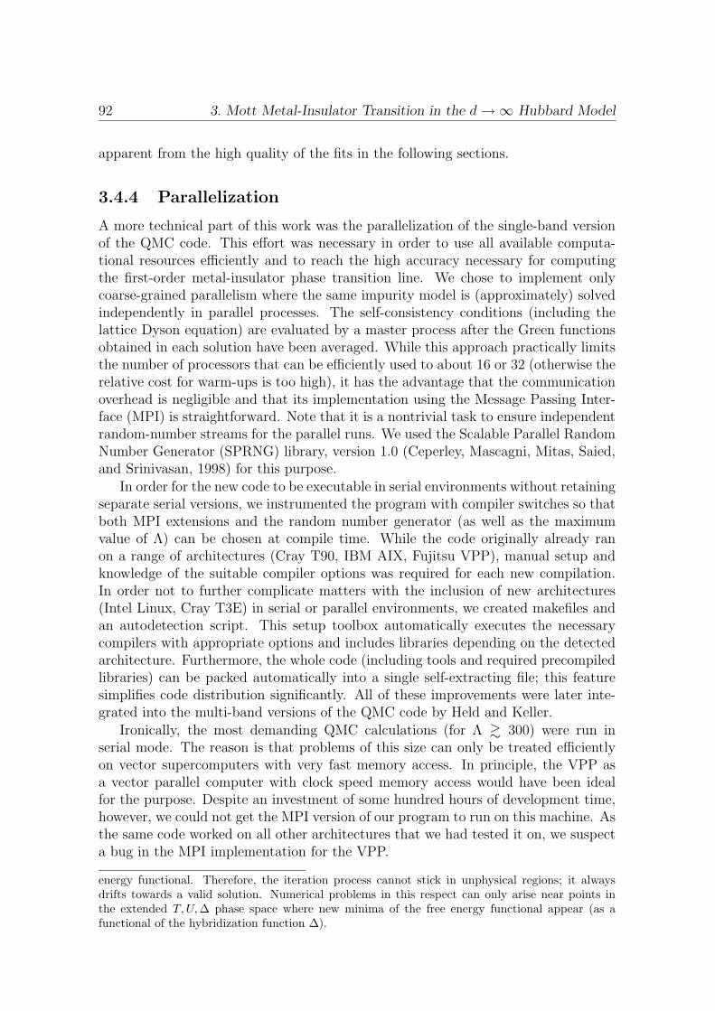
92 3. Mott Metal-Insulator Transition in the d→∞ Hubbard Model
apparent from the high quality of the fits in the following sections.
3.4.4 Parallelization
A more technical part of this work was the parallelization of the single-band versionof the QMC code. This effort was necessary in order to use all available computa-tional resources efficiently and to reach the high accuracy necessary for computingthe first-order metal-insulator phase transition line. We chose to implement onlycoarse-grained parallelism where the same impurity model is (approximately) solvedindependently in parallel processes. The self-consistency conditions (including thelattice Dyson equation) are evaluated by a master process after the Green functionsobtained in each solution have been averaged. While this approach practically limitsthe number of processors that can be efficiently used to about 16 or 32 (otherwise therelative cost for warm-ups is too high), it has the advantage that the communicationoverhead is negligible and that its implementation using the Message Passing Inter-face (MPI) is straightforward. Note that it is a nontrivial task to ensure independentrandom-number streams for the parallel runs. We used the Scalable Parallel RandomNumber Generator (SPRNG) library, version 1.0 (Ceperley, Mascagni, Mitas, Saied,and Srinivasan, 1998) for this purpose.
In order for the new code to be executable in serial environments without retainingseparate serial versions, we instrumented the program with compiler switches so thatboth MPI extensions and the random number generator (as well as the maximumvalue of Λ) can be chosen at compile time. While the code originally already ranon a range of architectures (Cray T90, IBM AIX, Fujitsu VPP), manual setup andknowledge of the suitable compiler options was required for each new compilation.In order not to further complicate matters with the inclusion of new architectures(Intel Linux, Cray T3E) in serial or parallel environments, we created makefiles andan autodetection script. This setup toolbox automatically executes the necessarycompilers with appropriate options and includes libraries depending on the detectedarchitecture. Furthermore, the whole code (including tools and required precompiledlibraries) can be packed automatically into a single self-extracting file; this featuresimplifies code distribution significantly. All of these improvements were later inte-grated into the multi-band versions of the QMC code by Held and Keller.
Ironically, the most demanding QMC calculations (for Λ & 300) were run inserial mode. The reason is that problems of this size can only be treated efficientlyon vector supercomputers with very fast memory access. In principle, the VPP asa vector parallel computer with clock speed memory access would have been idealfor the purpose. Despite an investment of some hundred hours of development time,however, we could not get the MPI version of our program to run on this machine. Asthe same code worked on all other architectures that we had tested it on, we suspecta bug in the MPI implementation for the VPP.
energy functional. Therefore, the iteration process cannot stick in unphysical regions; it alwaysdrifts towards a valid solution. Numerical problems in this respect can only arise near points inthe extended T,U,∆ phase space where new minima of the free energy functional appear (as afunctional of the hybridization function ∆).

3.5. Results: Coexistence Region 93
3.5 Results: Coexistence Region
In this section, we will begin the systematic construction of the phase diagram ofthe fully frustrated Hubbard model with semi-elliptic DOS in d→∞ at half filling.For this purpose, only those observables need to be considered which can be directlycomputed from standard QMC solutions of the DMFT self-consistency equations.As shown in subsection 3.5.1, the internal energy E is very well suited for determin-ing the metal-insulator transition in the physical limit ∆τ → 0, much better thanother observables considered so far. In subsection 3.5.2, we establish and parametrizeuniversal, i.e., temperature-independent, properties of the insulating phase. Measure-ments of the energy E presented in subsection 3.5.3 are used for the construction ofa preliminary phase diagram including a crossover region at high temperatures, acritical end point, and a region of coexisting metallic and insulating solutions at lowtemperatures in subsection 3.5.4.
Measurements of the double occupancy D and its (difficult) extrapolation for∆τ → 0 in the metallic phase are discussed in subsection 3.5.5. The very preciseextrapolated QMC estimates for E and D obtained in this section will allow for animplicit comparison of the free energies of the metal and the insulator (within thecoexistence region) and will lead to the full phase diagram in Sec. 3.6.
3.5.1 Choice of Observables and Extrapolation
In this subsection, we determine which of the observables introduced in subsection3.2.3 are best suited for indicating and characterizing the metal-insulator transition.Using QMC results for the relatively high temperature T = 1/15 ≈ 0.067 as a testcase, we discuss in particular the difficulties of extrapolations to the physical limit∆τ = 0.
The double occupancy for T = 0.067 is shown in Fig. 3.15 for a range of valuesof the discretization parameter ∆τ . Here, the symbols, which reflect QMC mea-surements, have been connected by straight line segments in order to guide the eye.As expected on physical grounds, the double occupancy decreases significantly withincreasing U , i.e., with decreasing metallicity. Evidently, the slope |dD/ dU | reachesa maximum at 4.55 . U . 4.65 (depending on ∆τ). One would be hard pressed,however, to decide if there is a continuous crossover or a sharp transition, even forfinite ∆τ . Furthermore, the dependence of D on ∆τ is seen to be very irregular:coming from the metallic side the ∆τ error increases up to U ≈ 4.6 while it is invis-ible on the insulating side.21 One might suspect that the primary effect of a finite∆τ error is a horizontal shift of the curves towards larger values of U . Still, resultsof an extrapolation to ∆τ = 0 would strongly depend on the assumed (nontrivial)functional forms and, thus, be unreliable without additional input.
A similar picture emerges for the quasiparticle weight Z as defined in (3.6) andshown in Fig. 3.16. This observable is in principle a very good candidate for char-acterizing the metal-insulator transition since, within the Fermi liquid picture, the
21The absence of significant ∆τ dependence for the QMC estimate of D in the insulator may bespecific to the particular algorithms used in our code.
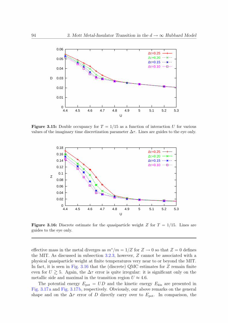
94 3. Mott Metal-Insulator Transition in the d→∞ Hubbard Model
0
0.01
0.02
0.03
0.04
0.05
0.06
4.4 4.5 4.6 4.7 4.8 4.9 5 5.1 5.2 5.3
D
U
∆τ=0.25∆τ=0.20∆τ=0.15∆τ=0.10
Figure 3.15: Double occupancy for T = 1/15 as a function of interaction U for variousvalues of the imaginary time discretization parameter ∆τ . Lines are guides to the eye only.
0
0.02
0.04
0.06
0.08
0.1
0.12
0.14
0.16
0.18
4.4 4.5 4.6 4.7 4.8 4.9 5 5.1 5.2 5.3
Z
U
∆τ=0.25∆τ=0.20∆τ=0.15∆τ=0.10
Figure 3.16: Discrete estimate for the quasiparticle weight Z for T = 1/15. Lines areguides to the eye only.
effective mass in the metal diverges as m∗/m = 1/Z for Z → 0 so that Z = 0 definesthe MIT. As discussed in subsection 3.2.3, however, Z cannot be associated with aphysical quasiparticle weight at finite temperatures very near to or beyond the MIT.In fact, it is seen in Fig. 3.16 that the (discrete) QMC estimates for Z remain finiteeven for U & 5. Again, the ∆τ error is quite irregular: it is significant only on themetallic side and maximal in the transition region U ≈ 4.6.
The potential energy Epot = UD and the kinetic energy Ekin are presented inFig. 3.17a and Fig. 3.17b, respectively. Obviously, our above remarks on the generalshape and on the ∆τ error of D directly carry over to Epot. In comparison, the
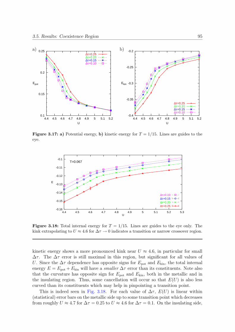
3.5. Results: Coexistence Region 95
a) b)
0.1
0.15
0.2
0.25
4.4 4.5 4.6 4.7 4.8 4.9 5 5.1 5.2
Epot
U
∆τ=0.25∆τ=0.20∆τ=0.15∆τ=0.10
-0.4
-0.35
-0.3
-0.25
-0.2
4.4 4.5 4.6 4.7 4.8 4.9 5 5.1 5.2
Ekin
U
∆τ=0.25∆τ=0.20∆τ=0.15∆τ=0.10
Figure 3.17: a) Potential energy, b) kinetic energy for T = 1/15. Lines are guides to theeye.
-0.16
-0.15
-0.14
-0.13
-0.12
-0.11
-0.1
4.4 4.5 4.6 4.7 4.8 4.9 5 5.1 5.2 5.3
E
U
T=0.067
∆τ=0.10∆τ=0.15∆τ=0.20∆τ=0.25
Figure 3.18: Total internal energy for T = 1/15. Lines are guides to the eye only. Thekink extrapolating to U ≈ 4.6 for ∆τ → 0 indicates a transition or narrow crossover region.
kinetic energy shows a more pronounced kink near U ≈ 4.6, in particular for small∆τ . The ∆τ error is still maximal in this region, but significant for all values ofU . Since the ∆τ dependence has opposite signs for Epot and Ekin, the total internalenergy E = Epot +Ekin will have a smaller ∆τ error than its constituents. Note alsothat the curvature has opposite sign for Epot and Ekin, both in the metallic and inthe insulating region. Thus, some cancellation will occur so that E(U) is also lesscurved than its constituents which may help in pinpointing a transition point.
This is indeed seen in Fig. 3.18. For each value of ∆τ , E(U) is linear within(statistical) error bars on the metallic side up to some transition point which decreasesfrom roughly U ≈ 4.7 for ∆τ = 0.25 to U ≈ 4.6 for ∆τ = 0.1. On the insulating side,
96 3. Mott Metal-Insulator Transition in the d→∞ Hubbard Model
the curves are again almost linear with significantly reduced slope; here, however,a small curvature remains visible. The comparatively sharp kinks unambiguouslyindicate the positions of phase transitions (or narrow crossover regions) for eachvalue of the time discretization ∆τ . A detailed analysis using suitable fit functionswill be presented in the next subsection. Furthermore, the dependence of the curveson ∆τ is very regular both on the metallic and on the insulating side. While wewill look at the precise extrapolation laws below, it is apparent from the figure thatthe ∆τ error is about a factor of 3/2 larger in the metallic phase. This explainsthe irregularity of the ∆τ dependence within the transition region where the phasetransition (or crossover) line is passed upon varying ∆τ for constant U . As longas this problematic region is excluded, very precise extrapolations ∆τ → 0 can beexpected. Finally, the regular shape of each curve also significantly reduces theconvergence error since measurements obtained from unconverged solutions can bedetected as deviations from the regular pattern and then corrected by performingadditional simulations.
If high-frequency tail corrections in the energy estimators are properly takeninto account (cf. subsection 3.2.3), low-frequency errors associated with the discreteFourier transforms (cf. subsection 3.4.1) are avoided, and no phase transition linesare crossed, the error in the estimate for E is dominated by the Trotter error (cf.Sec. 1.3) which is O(∆τ 2). Therefore, a reasonable starting point for a quantitativeanalysis is a purely quadratic extrapolation ∆τ → 0 (i.e., a linear least-squares fit in∆τ 2), both on the metallic and on the insulating side. The intersection of linear fitsfor Em(U) and Ei(U) of the metallic and insulating solution then determines a firstestimate of the transition point.
We found that the accuracy both in the estimates for energies and for transitionpoints could be improved by an order of magnitude by extending the least squaresfits to fourth order in ∆τ (i.e., by using fits of the form EU(∆τ) = EU(0) + c2∆τ
2 +c4∆τ
4) and by extracting a more complicated, more accurate, and thermodynamicallyconsistent expression for the energy in the insulator.
3.5.2 Properties of the Insulating Phase
Leaving properties of the metallic phase for the next subsections, we will now takea detailed look at the insulating phase. The symbols in Fig. 3.19 represent all ofour QMC measurements of E inside the insulating phase for various temperaturesT and interactions U as a function of ∆τ 2. The most important observation is theabsence of any significant dependence of E on T . Such universal behavior is expecteddeep inside the insulating low-temperature phase where a well-developed gap in thespectrum exists at the Fermi energy (cf. Sec. 3.8) and where thermal excitations aresuppressed exponentially. Evidently, the specific heat is already reduced by severalorders of magnitude compared to the metallic case in the low-temperature region ofinterest very close above the MIT as soon as a pseudo-gap appears. One practicalconsequence is that for fixed interaction U all QMC data points may be includedin a least squares fit for the extrapolation ∆τ → 0, irrespective of the associatedtemperature T . The solid lines in Fig. 3.19 reflect such extrapolations; here all three
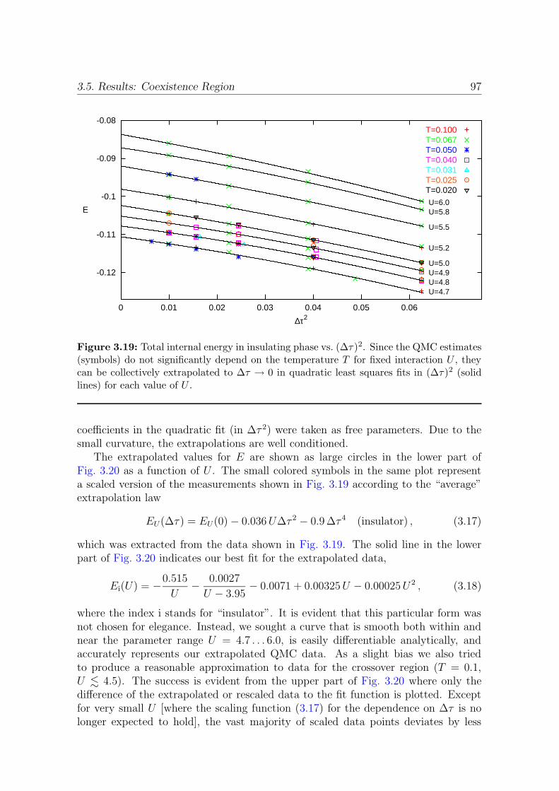
3.5. Results: Coexistence Region 97
-0.12
-0.11
-0.1
-0.09
-0.08
0 0.01 0.02 0.03 0.04 0.05 0.06
E
∆τ2
U=6.0U=5.8
U=5.5
U=5.2
U=5.0U=4.9U=4.8U=4.7
T=0.100T=0.067T=0.050T=0.040T=0.031T=0.025T=0.020
Figure 3.19: Total internal energy in insulating phase vs. (∆τ)2. Since the QMC estimates(symbols) do not significantly depend on the temperature T for fixed interaction U , theycan be collectively extrapolated to ∆τ → 0 in quadratic least squares fits in (∆τ)2 (solidlines) for each value of U .
coefficients in the quadratic fit (in ∆τ 2) were taken as free parameters. Due to thesmall curvature, the extrapolations are well conditioned.
The extrapolated values for E are shown as large circles in the lower part ofFig. 3.20 as a function of U . The small colored symbols in the same plot representa scaled version of the measurements shown in Fig. 3.19 according to the “average”extrapolation law
EU(∆τ) = EU(0)− 0.036U∆τ 2 − 0.9 ∆τ 4 (insulator) , (3.17)
which was extracted from the data shown in Fig. 3.19. The solid line in the lowerpart of Fig. 3.20 indicates our best fit for the extrapolated data,
Ei(U) = −0.515
U− 0.0027
U − 3.95− 0.0071 + 0.00325U − 0.00025U 2 , (3.18)
where the index i stands for “insulator”. It is evident that this particular form wasnot chosen for elegance. Instead, we sought a curve that is smooth both within andnear the parameter range U = 4.7 . . . 6.0, is easily differentiable analytically, andaccurately represents our extrapolated QMC data. As a slight bias we also triedto produce a reasonable approximation to data for the crossover region (T = 0.1,U . 4.5). The success is evident from the upper part of Fig. 3.20 where only thedifference of the extrapolated or rescaled data to the fit function is plotted. Exceptfor very small U [where the scaling function (3.17) for the dependence on ∆τ is nolonger expected to hold], the vast majority of scaled data points deviates by less
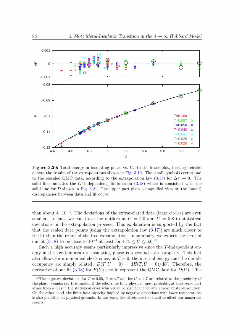
98 3. Mott Metal-Insulator Transition in the d→∞ Hubbard Model
-0.12
-0.11
-0.1
-0.09
-0.08
4.4 4.6 4.8 5 5.2 5.4 5.6 5.8 6
E
U
T=0.100T=0.067T=0.050T=0.040T=0.031T=0.025T=0.020
-0.001
0
0.001
∆E
Figure 3.20: Total energy in insulating phase vs. U . In the lower plot, the large circlesdenote the results of the extrapolations shown in Fig. 3.19. The small symbols correspondto the rescaled QMC data, according to the extrapolation law (3.17) for ∆τ → 0. Thesolid line indicates the (T -independent) fit function (3.18) which is consistent with thesolid line for D shown in Fig. 3.21. The upper part gives a magnified view on the (small)discrepancies between data and fit curve.
than about 4 · 10−4. The deviations of the extrapolated data (large circles) are evensmaller. In fact, we can trace the outliers at U = 5.0 and U = 5.8 to statisticaldeviations in the extrapolation process. This explanation is supported by the factthat the scaled data points [using the extrapolation law (3.17)] are much closer tothe fit than the result of the free extrapolation. In summary, we expect the error ofour fit (3.18) to be close to 10−4 at least for 4.75 ≤ U ≤ 6.0.22
Such a high accuracy seems particularly impressive since the T -independent en-ergy in the low-temperature insulating phase is a ground state property. This factalso allows for a numerical check since, at T = 0, the internal energy and the doubleoccupancy are simply related: D(T, U = 0) = dE(T, U = 0)/dU . Therefore, thederivative of our fit (3.18) for E(U) should represent the QMC data for D(U). This
22The negative deviations for T = 0.05, U = 4.7 and for U < 4.7 are related to the proximity ofthe phase boundaries. It is unclear if the effects are fully physical; most probably, at least some partarises from a bias in the statistical error which may be significant for any almost unstable solution.On the other hand, the finite heat capacity implied by negative deviations with lower temperaturesis also plausible on physical grounds. In any case, the effects are too small to affect our numericalresults.
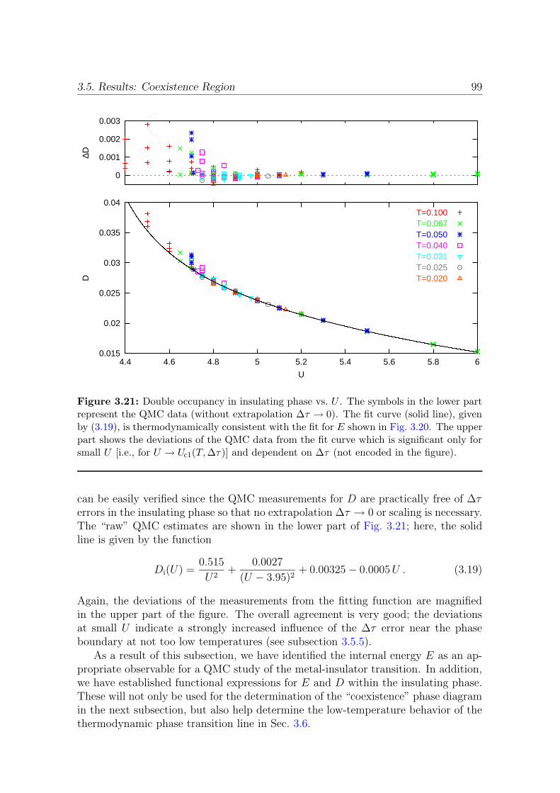
3.5. Results: Coexistence Region 99
0.015
0.02
0.025
0.03
0.035
0.04
4.4 4.6 4.8 5 5.2 5.4 5.6 5.8 6
D
U
T=0.100T=0.067T=0.050T=0.040T=0.031T=0.025T=0.020
0
0.001
0.002
0.003
∆D
Figure 3.21: Double occupancy in insulating phase vs. U . The symbols in the lower partrepresent the QMC data (without extrapolation ∆τ → 0). The fit curve (solid line), givenby (3.19), is thermodynamically consistent with the fit for E shown in Fig. 3.20. The upperpart shows the deviations of the QMC data from the fit curve which is significant only forsmall U [i.e., for U → Uc1(T,∆τ)] and dependent on ∆τ (not encoded in the figure).
can be easily verified since the QMC measurements for D are practically free of ∆τerrors in the insulating phase so that no extrapolation ∆τ → 0 or scaling is necessary.The “raw” QMC estimates are shown in the lower part of Fig. 3.21; here, the solidline is given by the function
Di(U) =0.515
U2+
0.0027
(U − 3.95)2+ 0.00325− 0.0005U . (3.19)
Again, the deviations of the measurements from the fitting function are magnifiedin the upper part of the figure. The overall agreement is very good; the deviationsat small U indicate a strongly increased influence of the ∆τ error near the phaseboundary at not too low temperatures (see subsection 3.5.5).
As a result of this subsection, we have identified the internal energy E as an ap-propriate observable for a QMC study of the metal-insulator transition. In addition,we have established functional expressions for E and D within the insulating phase.These will not only be used for the determination of the “coexistence” phase diagramin the next subsection, but also help determine the low-temperature behavior of thethermodynamic phase transition line in Sec. 3.6.

100 3. Mott Metal-Insulator Transition in the d→∞ Hubbard Model
3.5.3 Internal Energy
In the following, we present QMC data for the internal energy E, fits for finite ∆τ ,and extrapolations to the physical limit ∆τ = 0, ordered by decreasing temperature.The extrapolated data is summarized at the end of this subsection; the resultingphase diagram will be shown in the next subsection 3.5.4.
Since the insulating side has already been analyzed in the previous subsection,the remaining difficulty is the treatment of the metallic phase and the determinationof the phase boundaries. Within the metallic phase, we use quadratic least-squaresfits in ∆τ 2 for fixed U . Due to the small number of data points, the error in thequadratic coefficient (i.e., the ∆τ 4 term) is, however, of the same order of magnitudeas the estimate itself. Furthermore, the estimate may shift depending on whetheror not data points with small ∆τ are included. In order to minimize the resultingerrors, we have assumed slow variation of this coefficient as a function of U and Tand have performed a global fit. The result is that the ∆τ 4 coefficient for the metalis always close to the value 0.95 computed for the insulating phase. The observationof a slight variation as a function of T lead to a linear interpolation with a value of1.2 for T = 0.1 and 0.8 for T = 0.02.23 This coefficient was then held fixed for allextrapolations within the metallic phase.
The results of such extrapolations to ∆τ = 0 at T = 0.1, the highest temperatureconsidered here, are denoted as solid circles in Fig. 3.22. The ∆τ = 0 values forU = 4.1, U = 4.2, and U = 4.3 fall on a straight line which extends to U = 4.4 and ispartially drawn as a thick and partially as a thin line. The parallel lines connectingdata points for finite ∆τ are offset according to a scaling law which not only includesthe globally determined ∆τ 4 coefficient, but also a ∆τ 2 coefficient which has beenaveraged from the extrapolations for U = 4.1, U = 4.2, and U = 4.3. Each of these“metallic” lines crosses the corresponding “insulating” line (beginning as thick curveat large U and extending into a thin line towards the metallic phase) at some point.In this region, however, the QMC data deviates systematically from the fit curves,indicating a smooth crossover rather than a phase transition.24
An analogous plot for T = 0.067 (more accurately: β = 15, i.e., T = 1/15) isshown in Fig. 3.23.25 Here, the transition is (almost) sharp within the numericalaccuracy, i.e., the data follows linear fits in the metallic phase and the universal form(3.18) in connection with (3.17) in the insulating phase, respectively, for all valuesof the interaction U . Consequently, the transition points can be determined and ex-trapolated very accurately: Uc = 4.59. Only extremely close to the transition points,i.e., for U = 4.65 at ∆τ = 0.15 and U = 4.7 at ∆τ = 0.2, do slight deviations of theQMC data from the fits indicate some rounding effect. This observation, in combina-tion with conclusions from lower temperatures, will later lead to the conclusion thatT = 0.067 is close to, but slightly above, the critical temperature.
23Note that while the relative error for the coefficient is relatively large, its influence is small.The intrinsic uncertainty of about 0.2 translates, e.g., into a possible additional error in the energyestimates of 2 · 10−5 for ∆τ = 0.1 and 3 · 10−4 for ∆τ = 0.2.
24As the precise behavior of E in the crossover region will be irrelevant in the following, we onlysketched the assumed form by manually adapting cubic splines (thick lines).
25Compare also the data for this temperature shown in the previous subsection.
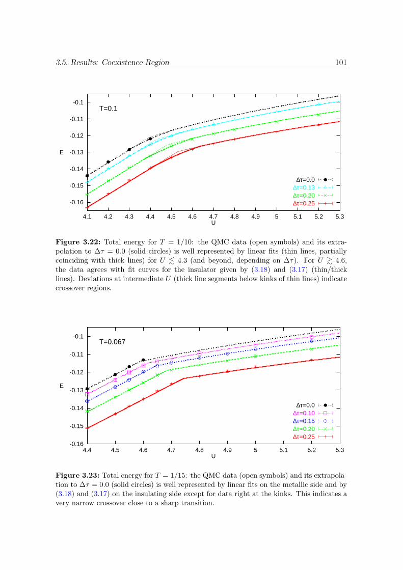
3.5. Results: Coexistence Region 101
-0.16
-0.15
-0.14
-0.13
-0.12
-0.11
-0.1
4.1 4.2 4.3 4.4 4.5 4.6 4.7 4.8 4.9 5 5.1 5.2 5.3
E
U
T=0.1
∆τ=0.0∆τ=0.13∆τ=0.20∆τ=0.25
Figure 3.22: Total energy for T = 1/10: the QMC data (open symbols) and its extra-polation to ∆τ = 0.0 (solid circles) is well represented by linear fits (thin lines, partiallycoinciding with thick lines) for U . 4.3 (and beyond, depending on ∆τ). For U & 4.6,the data agrees with fit curves for the insulator given by (3.18) and (3.17) (thin/thicklines). Deviations at intermediate U (thick line segments below kinks of thin lines) indicatecrossover regions.
-0.16
-0.15
-0.14
-0.13
-0.12
-0.11
-0.1
4.4 4.5 4.6 4.7 4.8 4.9 5 5.1 5.2 5.3
E
U
T=0.067
∆τ=0.0∆τ=0.10∆τ=0.15∆τ=0.20∆τ=0.25
Figure 3.23: Total energy for T = 1/15: the QMC data (open symbols) and its extrapola-tion to ∆τ = 0.0 (solid circles) is well represented by linear fits on the metallic side and by(3.18) and (3.17) on the insulating side except for data right at the kinks. This indicates avery narrow crossover close to a sharp transition.

102 3. Mott Metal-Insulator Transition in the d→∞ Hubbard Model
-0.17
-0.16
-0.15
-0.14
-0.13
-0.12
-0.11
4.2 4.3 4.4 4.5 4.6 4.7 4.8 4.9 5 5.1
E
U
T=0.05
∆τ=0.0∆τ=0.10∆τ=0.13∆τ=0.16∆τ=0.20∆τ=0.25
-0.13
-0.12
-0.11
-0.1
E
T=0.05
Figure 3.24: Total energy for T = 1/20: in order to avoid confusion within the coexistenceregion, QMC data for the metallic phase is presented in the lower plot and the data for theinsulator in the upper plot (with identical scales). As in the previous plots, the fit functionsfor the insulating phase (thick lines in upper plot) have the universal form given by (3.18)and (3.17); their extent reflects our estimate of its stability region. In the lower plot, thelinear fits for the metal are drawn as thick lines below Uc2, where the metallic phase isstable, but extended as thin lines up to Uc2b, where they cross the corresponding fit for theinsulator.
In contrast, a small coexistence region of metallic and insulating solution appearsfor T = 0.05 as shown in Fig. 3.24. Here, we have split the presentation of theQMC data for the metallic phase (lower part) and insulating phase (upper part).The fit curves are repeated in both parts with emphasis (thick lines) on the phaseunder consideration. While the extent of the fit curves for the insulator reflectsour estimate of the extent of its stability region (which depends on ∆τ), the metalliccurves are always drawn until they cross the corresponding insulating solutions. Thesecrossing points, which can be determined with great precision, will later be used asparameters for fitting the double occupancy. The metallic curves are drawn as thicklines within (our estimate of) their stability range. Note that the QMC data generallyagrees well with the fit curves; only right at the stability edges, systematic deviationstowards the more stable phase are seen. While it is plausible that this effect might bepartially genuine, we observed that it can be reduced by improving the accuracy of
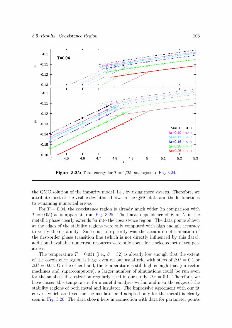
3.5. Results: Coexistence Region 103
-0.16
-0.15
-0.14
-0.13
-0.12
-0.11
-0.1
4.4 4.5 4.6 4.7 4.8 4.9 5 5.1 5.2 5.3
E
U
T=0.04
∆τ=0.0∆τ=0.10∆τ=0.13∆τ=0.16∆τ=0.20∆τ=0.25
-0.13
-0.12
-0.11
-0.1
E
T=0.04
Figure 3.25: Total energy for T = 1/25, analogous to Fig. 3.24.
the QMC solution of the impurity model, i.e., by using more sweeps. Therefore, weattribute most of the visible deviations between the QMC data and the fit functionsto remaining numerical errors.
For T = 0.04, the coexistence region is already much wider (in comparison withT = 0.05) as is apparent from Fig. 3.25. The linear dependence of E on U in themetallic phase clearly extends far into the coexistence region. The data points shownat the edges of the stability regions were only computed with high enough accuracyto verify their stability. Since our top priority was the accurate determination ofthe first-order phase transition line (which is not directly influenced by this data),additional available numerical resources were only spent for a selected set of temper-atures.
The temperature T = 0.031 (i.e., β = 32) is already low enough that the extentof the coexistence region is large even on our usual grid with steps of ∆U = 0.1 or∆U = 0.05. On the other hand, the temperature is still high enough that (on vectormachines and supercomputers), a larger number of simulations could be run evenfor the smallest discretization regularly used in our study, ∆τ = 0.1. Therefore, wehave chosen this temperature for a careful analysis within and near the edges of thestability regions of both metal and insulator. The impressive agreement with our fitcurves (which are fixed for the insulator and adapted only for the metal) is clearlyseen in Fig. 3.26. The data shown here in connection with data for parameter points
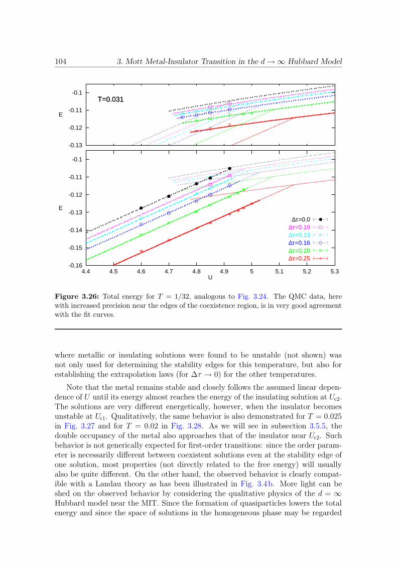
104 3. Mott Metal-Insulator Transition in the d→∞ Hubbard Model
-0.16
-0.15
-0.14
-0.13
-0.12
-0.11
-0.1
4.4 4.5 4.6 4.7 4.8 4.9 5 5.1 5.2 5.3
E
U
T=0.031
∆τ=0.0∆τ=0.10∆τ=0.13∆τ=0.16∆τ=0.20∆τ=0.25
-0.13
-0.12
-0.11
-0.1
E
T=0.031
Figure 3.26: Total energy for T = 1/32, analogous to Fig. 3.24. The QMC data, herewith increased precision near the edges of the coexistence region, is in very good agreementwith the fit curves.
where metallic or insulating solutions were found to be unstable (not shown) wasnot only used for determining the stability edges for this temperature, but also forestablishing the extrapolation laws (for ∆τ → 0) for the other temperatures.
Note that the metal remains stable and closely follows the assumed linear depen-dence of U until its energy almost reaches the energy of the insulating solution at Uc2.The solutions are very different energetically, however, when the insulator becomesunstable at Uc1. Qualitatively, the same behavior is also demonstrated for T = 0.025in Fig. 3.27 and for T = 0.02 in Fig. 3.28. As we will see in subsection 3.5.5, thedouble occupancy of the metal also approaches that of the insulator near Uc2. Suchbehavior is not generically expected for first-order transitions: since the order param-eter is necessarily different between coexistent solutions even at the stability edge ofone solution, most properties (not directly related to the free energy) will usuallyalso be quite different. On the other hand, the observed behavior is clearly compat-ible with a Landau theory as has been illustrated in Fig. 3.4b. More light can beshed on the observed behavior by considering the qualitative physics of the d = ∞Hubbard model near the MIT. Since the formation of quasiparticles lowers the totalenergy and since the space of solutions in the homogeneous phase may be regarded
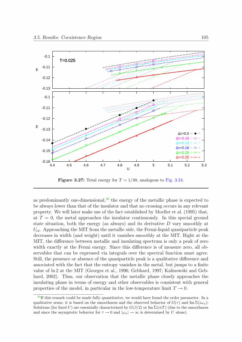
3.5. Results: Coexistence Region 105
-0.16
-0.15
-0.14
-0.13
-0.12
-0.11
-0.1
4.4 4.5 4.6 4.7 4.8 4.9 5 5.1 5.2 5.3
E
U
T=0.025
∆τ=0.0∆τ=0.10∆τ=0.13∆τ=0.16∆τ=0.20∆τ=0.25
-0.13
-0.12
-0.11
-0.1
E
T=0.025
Figure 3.27: Total energy for T = 1/40, analogous to Fig. 3.24.
as predominantly one-dimensional,26 the energy of the metallic phase is expected tobe always lower than that of the insulator and that no crossing occurs in any relevantproperty. We will later make use of the fact established by Moeller et al. (1995) that,at T = 0, the metal approaches the insulator continuously. In this special groundstate situation, both the energy (as always) and its derivative D vary smoothly atUc2. Approaching the MIT from the metallic side, the Fermi-liquid quasiparticle peakdecreases in width (and weight) until it vanishes smoothly at the MIT. Right at theMIT, the difference between metallic and insulating spectrum is only a peak of zerowidth exactly at the Fermi energy. Since this difference is of measure zero, all ob-servables that can be expressed via integrals over the spectral function must agree.Still, the presence or absence of the quasiparticle peak is a qualitative difference andassociated with the fact that the entropy vanishes in the metal, but jumps to a finitevalue of ln 2 at the MIT (Georges et al., 1996; Gebhard, 1997; Kalinowski and Geb-hard, 2002). Thus, our observation that the metallic phase closely approaches theinsulating phase in terms of energy and other observables is consistent with generalproperties of the model, in particular in the low-temperature limit T → 0.
26If this remark could be made fully quantitative, we would have found the order parameter. In aqualitative sense, it is based on the smoothness and the observed behavior of G(τ) and Im Σ(iωn):Solutions (for fixed U) are essentially characterized by G(β/2) or Im Σ(iπT ) (due to the smoothnessand since the asymptotic behavior for τ → 0 and |ωn| → ∞ is determined by U alone).

106 3. Mott Metal-Insulator Transition in the d→∞ Hubbard Model
-0.16
-0.15
-0.14
-0.13
-0.12
-0.11
-0.1
4.4 4.5 4.6 4.7 4.8 4.9 5 5.1 5.2 5.3
E
U
T=0.02
∆τ=0.0∆τ=0.13∆τ=0.16∆τ=0.20∆τ=0.25
-0.13
-0.12
-0.11
-0.1
E
T=0.02
Figure 3.28: Total energy for T = 1/50, analogous to Fig. 3.24.
Figure 3.27 shows results for T = 0.025 and includes data (for ∆τ = 0.1) withL = 400 time slices which was the maximum used in this study and is significantlylarger than values previously reported in the literature. Again, the agreement withthe fit curves is seen to be very good. Note that Uc1, the stability edge for theinsulator, agrees with the estimate obtained for T = 1/32. In contrast, lowering Tsignificantly reduces the energy of the metallic phase as the specific heat is then verysignificant. Therefore, Uc2, the stability edge of the metal, and Uc2b, the point wherethe extrapolated energies of metallic and insulating phases cross, further increaseupon lowering T .
These trends continue for T = 1/50 as seen in Fig. 3.28. At this temperature,no simulations can be performed at ∆τ = 0.1; instead the maximal number of timeslices is limited27 to Λ = 400 leading to ∆τ ≥ 0.125 ≈ 0.13. Since the temperature-independence of the energy in the insulating phase has already been established insubsection 3.5.2, the number of data points in this phase is kept to a minimum and thenumerical effort is concentrated instead on the metallic phase within the coexistence
27Note that the scaling of the computational effort as Λ3 established in Sec. 1.3 is only validfor supercomputers where the memory system works at cpu speed. For regular workstations, thescaling at large Λ is closer to Λ4 so that the computational cost for Λ = 400 is already more thantwo orders of magnitude higher than for Λ = 100, e.g., for ∆τ = 0.1 at T = 0.1. See also subsection1.3.2.
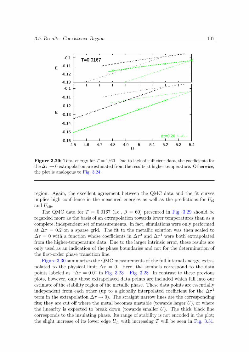
3.5. Results: Coexistence Region 107
-0.16
-0.15
-0.14
-0.13
-0.12
-0.11
-0.1
4.5 4.6 4.7 4.8 4.9 5 5.1 5.2 5.3 5.4
E
U
T=0.0167
∆τ=0.20
-0.13
-0.12
-0.11
-0.1
E
T=0.0167
Figure 3.29: Total energy for T = 1/60. Due to lack of sufficient data, the coefficients forthe ∆τ → 0 extrapolation are estimated from the results at higher temperature. Otherwise,the plot is analogous to Fig. 3.24.
region. Again, the excellent agreement between the QMC data and the fit curvesimplies high confidence in the measured energies as well as the predictions for Uc2
and Uc2b.
The QMC data for T = 0.0167 (i.e., β = 60) presented in Fig. 3.29 should beregarded more as the basis of an extrapolation towards lower temperatures than as acomplete, independent set of measurements. In fact, simulations were only performedat ∆τ = 0.2 on a sparse grid. The fit to the metallic solution was then scaled to∆τ = 0 with a function whose coefficients in ∆τ 2 and ∆τ 4 were both extrapolatedfrom the higher-temperature data. Due to the larger intrinsic error, these results areonly used as an indication of the phase boundaries and not for the determination ofthe first-order phase transition line.
Figure 3.30 summarizes the QMC measurements of the full internal energy, extra-polated to the physical limit ∆τ = 0. Here, the symbols correspond to the datapoints labeled as “∆τ = 0.0” in Fig. 3.23 – Fig. 3.28. In contrast to these previousplots, however, only those extrapolated data points are included which fall into ourestimate of the stability region of the metallic phase. These data points are essentiallyindependent from each other (up to a globally interpolated coefficient for the ∆τ 4
term in the extrapolation ∆τ → 0). The straight narrow lines are the correspondingfits; they are cut off where the metal becomes unstable (towards larger U), or wherethe linearity is expected to break down (towards smaller U). The thick black linecorresponds to the insulating phase. Its range of stability is not encoded in the plot;the slight increase of its lower edge Uc1 with increasing T will be seen in Fig. 3.31.
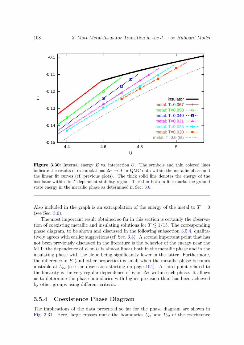
108 3. Mott Metal-Insulator Transition in the d→∞ Hubbard Model
-0.15
-0.14
-0.13
-0.12
-0.11
-0.1
4.4 4.6 4.8 5
E
U
insulatormetal: T=0.067metal: T=0.050metal: T=0.040metal: T=0.031metal: T=0.025metal: T=0.020
metal: T=0.0 (fit)
Figure 3.30: Internal energy E vs. interaction U . The symbols and thin colored linesindicate the results of extrapolations ∆τ → 0 for QMC data within the metallic phase andthe linear fit curves (cf. previous plots). The thick solid line denotes the energy of theinsulator within its T -dependent stability region. The thin bottom line marks the groundstate energy in the metallic phase as determined in Sec. 3.6.
Also included in the graph is an extrapolation of the energy of the metal to T = 0(see Sec. 3.6).
The most important result obtained so far in this section is certainly the observa-tion of coexisting metallic and insulating solutions for T . 1/15. The correspondingphase diagram, to be shown and discussed in the following subsection 3.5.4, qualita-tively agrees with earlier suggestions (cf. Sec. 3.3). A second important point that hasnot been previously discussed in the literature is the behavior of the energy near theMIT: the dependence of E on U is almost linear both in the metallic phase and in theinsulating phase with the slope being significantly lower in the latter. Furthermore,the difference in E (and other properties) is small when the metallic phase becomesunstable at Uc2 (see the discussion starting on page 104). A third point related tothe linearity is the very regular dependence of E on ∆τ within each phase. It allowsus to determine the phase boundaries with higher precision than has been achievedby other groups using different criteria.
3.5.4 Coexistence Phase Diagram
The implications of the data presented so far for the phase diagram are shown inFig. 3.31. Here, large crosses mark the boundaries Uc1 and Uc2 of the coexistence
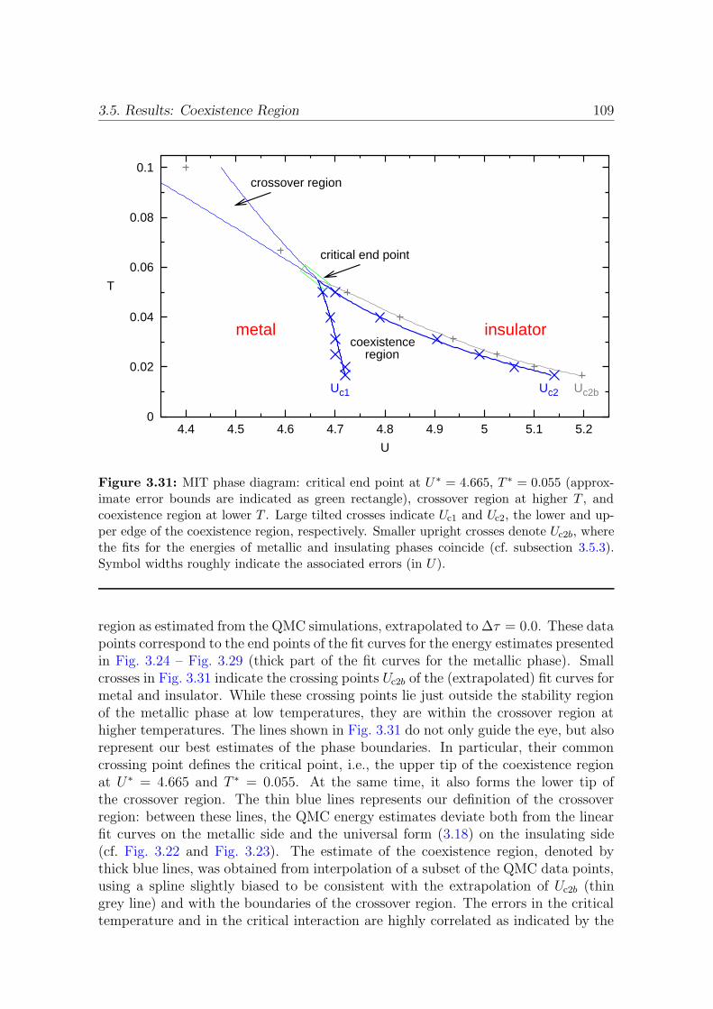
3.5. Results: Coexistence Region 109
0
0.02
0.04
0.06
0.08
0.1
4.4 4.5 4.6 4.7 4.8 4.9 5 5.1 5.2
T
U
metal insulator
crossover region
coexistenceregion
critical end point
Uc1 Uc2 Uc2b
Figure 3.31: MIT phase diagram: critical end point at U ∗ = 4.665, T ∗ = 0.055 (approx-imate error bounds are indicated as green rectangle), crossover region at higher T , andcoexistence region at lower T . Large tilted crosses indicate Uc1 and Uc2, the lower and up-per edge of the coexistence region, respectively. Smaller upright crosses denote Uc2b, wherethe fits for the energies of metallic and insulating phases coincide (cf. subsection 3.5.3).Symbol widths roughly indicate the associated errors (in U).
region as estimated from the QMC simulations, extrapolated to ∆τ = 0.0. These datapoints correspond to the end points of the fit curves for the energy estimates presentedin Fig. 3.24 – Fig. 3.29 (thick part of the fit curves for the metallic phase). Smallcrosses in Fig. 3.31 indicate the crossing points Uc2b of the (extrapolated) fit curves formetal and insulator. While these crossing points lie just outside the stability regionof the metallic phase at low temperatures, they are within the crossover region athigher temperatures. The lines shown in Fig. 3.31 do not only guide the eye, but alsorepresent our best estimates of the phase boundaries. In particular, their commoncrossing point defines the critical point, i.e., the upper tip of the coexistence regionat U ∗ = 4.665 and T ∗ = 0.055. At the same time, it also forms the lower tip ofthe crossover region. The thin blue lines represents our definition of the crossoverregion: between these lines, the QMC energy estimates deviate both from the linearfit curves on the metallic side and the universal form (3.18) on the insulating side(cf. Fig. 3.22 and Fig. 3.23). The estimate of the coexistence region, denoted bythick blue lines, was obtained from interpolation of a subset of the QMC data points,using a spline slightly biased to be consistent with the extrapolation of Uc2b (thingrey line) and with the boundaries of the crossover region. The errors in the criticaltemperature and in the critical interaction are highly correlated as indicated by the
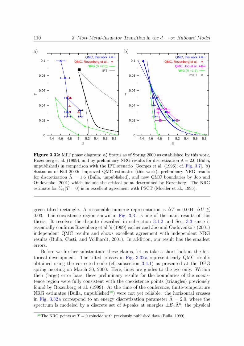
110 3. Mott Metal-Insulator Transition in the d→∞ Hubbard Model
a) b)
0
0.02
0.04
0.06
0.08
0.1
4.4 4.6 4.8 5 5.2 5.4 5.6 5.8
T
U
QMC, this workQMC, Rozenberg et al.
NRG (~Λ =2.0)IPT
0
0.02
0.04
0.06
0.08
0.1
4.4 4.6 4.8 5 5.2 5.4 5.6 5.8
T
U
QMC, this workQMC, Rozenberg et al.
QMC, Joo et al.NRG (~Λ =1.6)
PSCT
Figure 3.32: MIT phase diagram: a) Status as of Spring 2000 as established by this work,Rozenberg et al. (1999), and by preliminary NRG results for discretization Λ = 2.0 (Bulla,unpublished) in comparison with the IPT scenario [Georges et al. (1996); cf. Fig. 3.7]. b)Status as of Fall 2000: improved QMC estimates (this work), preliminary NRG resultsfor discretization Λ = 1.6 (Bulla, unpublished), and new QMC boundaries by Joo andOudovenko (2001) which include the critical point determined by Rozenberg. The NRGestimate for Uc2(T = 0) is in excellent agreement with PSCT (Moeller et al., 1995).
green tilted rectangle. A reasonable numeric representation is ∆T = 0.004, ∆U .
0.03. The coexistence region shown in Fig. 3.31 is one of the main results of thisthesis: It resolves the dispute described in subsection 3.1.2 and Sec. 3.3 since itessentially confirms Rozenberg et al.’s (1999) earlier and Joo and Oudovenko’s (2001)independent QMC results and shows excellent agreement with independent NRGresults (Bulla, Costi, and Vollhardt, 2001). In addition, our result has the smallesterrors.
Before we further substantiate these claims, let us take a short look at the his-torical development. The tilted crosses in Fig. 3.32a represent early QMC resultsobtained using the corrected code (cf. subsection 3.4.1) as presented at the DPGspring meeting on March 30, 2000. Here, lines are guides to the eye only. Withintheir (large) error bars, these preliminary results for the boundaries of the coexis-tence region were fully consistent with the coexistence points (triangles) previouslyfound by Rozenberg et al. (1999). At the time of the conference, finite-temperatureNRG estimates (Bulla, unpublished28) were not yet reliable: the horizontal crossesin Fig. 3.32a correspond to an energy discretization parameter Λ = 2.0, where thespectrum is modeled by a discrete set of δ-peaks at energies ±E0 Λn; the physical
28The NRG points at T = 0 coincide with previously published data (Bulla, 1999).

3.5. Results: Coexistence Region 111
continuum limit is recovered for Λ → 1. Attributing the differences between NRGand QMC to the known systematic underestimation of critical interactions by NRGat large Λ (and finite temperature), the agreement appeared reasonable, in particularwhen compared with IPT (thin lines).
Figure 3.32b represents the status of the phase diagram of late October 2000.29
Here, our QMC estimates (crosses) are already based on measurements of the fullinternal energy (cf. subsection 3.5.1). This fact and a large number of simulationson a finer grid result in an accuracy which is much higher than that of the prelimi-nary results shown in Fig. 3.32a and also significantly higher than that of Joo andOudovenko’s (2001) results shown as squares in Fig. 3.32b (which were first availableas preprints in late September 2000).30 The surprisingly good agreement betweenour QMC results and the improved NRG results [which are close to, but not identicalwith the data shown in the subsequent publication (Bulla et al., 2001)] is partiallyaccidental as the final results for QMC and NRG show slightly larger differences (cf.subsection 3.6.3). Still, the good overall agreement between these results and (withinlarger error bars) with the independent QMC results obtained by Joo and Oudovenko(2001) indicated a resolution of the controversy towards a reliable phase diagram. Inparticular, the improved NRG estimate Uc2(T = 0) = 5.86 is practically identical withthe PSCT/ED estimate Uc2(T = 0) = 5.84. These and all other published numericalestimates for the boundaries of the MIT coexistence region at T = 0 that we areaware of are reproduced in Table 3.1. A corresponding summary for the coordinatesof the second-order critical end point is given in Table 3.2; the latter also includesour new QMC estimate.
The thick line in Fig. 3.32b which evolves into a dashed line at low temperaturesreflects our estimate (as of October 2000) of the true first-order phase transition line;the final estimate (which is hardly distinguishable from the curve shown here) willbe presented after detailing the methodology in Sec. 3.6. The low-temperature partof this curve is partially based on the assumption that Uc2(T = 0) ≈ 5.85 which iscertainly justified based on the excellent agreement between PSCT, ED, and NRG.
Leaving the historical review, let us discuss the possible origin of the remainingdiscrepancies between the various QMC estimates of the boundaries of the coexis-tence region. Tilted and upright crosses in Fig. 3.33 represent our extrapolated QMCdata (here repeated from Fig. 3.31) and QMC data corresponding to ∆τ = 0.25, re-spectively. Evidently, the extrapolation ∆τ → 0 is important; otherwise (i.e., at∆τ = 0.25), the coexistence region is shifted by about ∆U ≈ 0.1 towards largerinteraction and by about ∆T ≈ 0.005 towards higher temperatures.31 Interestingly,
29The comparison shown here was prepared for a conference in Grenoble (starting on October 30,2000); on that occasion, a paper copy was also handed out to Georges. The same data (includingour estimate for the first-order phase transition line) was presented in talks in condensed mattertheory seminars in Augsburg and Mainz on 11/29/00 and 12/05/00, respectively and appeared ina report sent to the van Neumann Institute for Computing in November 2000.
30Note that Joo and Oudovenko (2001) did not calculate the tip of the coexistence region. Instead,they used Rozenberg et al.’s (1999) earlier estimate.
31Note that in our computations, the range of discretization parameters includes 0.1 ≤ ∆τ ≤ 0.25even for relatively low temperatures T ≥ 0.025 (∆τmin = 0.125 for T = 0.02). Therefore, thedeviation of our best “raw” results from the extrapolated results is much smaller than shown in this

112 3. Mott Metal-Insulator Transition in the d→∞ Hubbard Model
Uc1 Uc2 method factor citation
5.1 6.6 IPT√
2 Georges and Krauth (1993), p. 71725.2 6.6 IPT 2 Rozenberg et al. (1994), Fig. 104.7 QMC 2 Rozenberg et al. (1994), p. 10186
5.8 PSCT 2 Moeller et al. (1995), p. 20844.3± 0.5 5.84± 0.1 ED,PSCT 2D Georges et al. (1996), p. 664.0± 0.4 4.0± 0.4 RDA+ED 4W Noack and Gebhard (1999), p. 19175 5.88 NRG 4W Bulla (1999), p. 138/1374.78 5.86 NRG 4W Bulla et al. (2001), p. 8, Fig. 9
Table 3.1: MIT at T = 0 in the half-filled fully frustrated Hubbard model with semi-elliptic DOS for d → ∞. All values for Uc1 and Uc2 have been rescaled to unit varianceof the DOS by multiplying the values stated in the publications by the appropriate factor(fourth column).
U∗ T ∗ method citation
5.02 0.088 IPT Rozenberg et al. (1994), Fig. 104.76± 0.04 0.052± 0.006 QMC Rozenberg et al. (1999), p. 35004.9263 0.09379 IPT Kotliar et al. (2000), Fig. 24.68 0.050 ED Tong, Shen, and Pu (2001), p. 3
0.08 NRG Bulla et al. (2001), p. 6
4.665± 0.03 0.055± 0.004 QMC this work
Table 3.2: Second order critical end point of the MIT in the half-filled fully frustratedHubbard model with semi-elliptic DOS for d → ∞. Rescaling to unit variance requiredmultiplication by a factor of 4W for NRG and a factor of 2 for the other cited results.
our estimates for ∆τ = 0.25 practically match the final results published by Joo andOudovenko (2001) and are fully consistent with Rozenberg et al.’s (1999) data. Incontrast, the agreement between the published data and our extrapolated estimatesis much worse. In fact, no extrapolation is mentioned in Rozenberg et al.’s (1999)paper and an extrapolation ∆τ → 0 is explicitly stated only for two selected phasepoints by Joo and Oudovenko (2001). We stress that (at ∆τ = 0.0) the metallicsolution is not stable at four out of six points where coexistence has been claimedby Rozenberg et al. (1999). Thus, this paper contains quantitative errors; even itsqualitative correctness, i.e., the evidence for the existence of a coexistence region (at∆τ = 0.0) cannot be derived from data shown in the publication. Only our work,Joo and Oudovenko’s (2001) selective ∆τ studies, and Bulla’s NRG results demon-strate that among the various scenarios shown in Fig. 3.13 for the ∆τ dependence of
comparison. However, Rozenberg et al.’s (1999) best calculations at T = 0.031 were performed with∆τ = 0.25 and the same can be assumed for the bulk of Joo and Oudovenko’s (2001) calculations.

3.5. Results: Coexistence Region 113
0
0.02
0.04
0.06
4.7 4.8 4.9 5 5.1 5.2 5.3
T
U
∆τ=0.0
∆τ=0.25
Joo et al.
Rozenberg et al.
Figure 3.33: MIT phase diagram: dependency of the boundaries Uc1(T ) and Uc2(T ) ofthe coexistence region on ∆τ . Final results of this work for ∆τ = 0.0 (already shown inFig. 3.31) and ∆τ = 0.25 in comparison with Joo and Oudovenko’s (2001) results and thecoexistence points established by Rozenberg et al. (1999).
the coexistence region which appear a priori possible, the scenario of Fig. 3.13a isrealized: finite ∆τ primarily shifts the coexistence region towards larger values of U .Consequently, the coexistence found by Rozenberg can now a posteriori be assessedas genuine (and not as an artifact of using finite ∆τ).
Another fact established by these recent studies is that Uc1 is almost independentof T , only slightly increasing when the temperature is lowered from T = T ∗ to T = 0.This finding is clearly incompatible with the MIT scenario Fig. 3.10 suggested byKotliar which partially reconciled QMC results (at relatively high temperature) with(zero-temperature) RDA results by assuming that Uc1(T = 0) = 4.0. Ironically,our correction of this perception of the shape of the coexistence region validates aposteriori the qualitative features of the IPT scenario (cf. Fig. 3.7 and Fig. 3.32),originally supported by Kotliar (and others).
3.5.5 Double Occupancy
In this subsection, we construct an extrapolation scheme for the double occupancyD in the metallic phase. In connection with the expression (3.19) established forthe double occupancy of the insulating phase in subsection 3.5.1, the resulting esti-mates will allow for a determination of the difference ∆D(T, U) in double occupancybetween metal and insulator within a few percent. This data will be used in com-bination with corresponding estimates energetic differences ∆E(T, U) (obtained insubsection 3.5.3) for the construction of a differential equation governing the ther-modynamic first-order phase transition line Uc(T ) in Sec. 3.6. In addition to our best

114 3. Mott Metal-Insulator Transition in the d→∞ Hubbard Model
0.03
0.04
0.05
0.06
0.07
0.08
0.09
0.1
0 0.05 0.1 0.15 0.2 0.25
∆τ
D
T=0.04U=4.4U=4.6U=4.7
U=4.75U=4.8
0
0.1
0.2
0.3
4.4 4.5 4.6 4.7 4.8
U
d2 D /
d∆τ2
T=0.04
Figure 3.34: Extrapolation ∆τ → 0 of double occupancy D in metallic phase for T = 0.04:At small enough U , the QMC data points agree with purely quadratic least-squares fits(lines). Since the quadratic (in ∆τ) extrapolation law is seen to break down for U = 4.8,it is also unreliable at slightly smaller U . The inset shows the (second order) fit coefficientwhich increases significantly for U → Uc2.
estimate for the double occupancy in the metal, we will also indicate approximatefunctional forms for Dm(T, U) within the coexistence region which correspond exactlyto a linearized, interpolated version of this differential equation.
The difficulty in extrapolating D to the physical limit ∆τ → 0 is illustrated forT = 0.04 in Fig. 3.34. Well within the metallic phase, the dependence of D on∆τ follows quadratic fit curves (i.e., without linear terms). Within the range of ∆τshown in the plot, this observation even remains true (with strongly increased ∆τdependence; see inset of Fig. 3.34) up to U = 4.75. This value of the interaction is justbelow Uc2 = 4.8, where the metallic phase becomes unstable, and Uc2b ≈ 4.83, wherethe extrapolated energy (see Fig. 3.25) meets that of the insulator. At U = 4.8,however, the purely quadratic extrapolation law for the double occupancy clearlybreaks down for ∆τ . 0.16. The observed irregularity not only makes it impossibleto perform the extrapolation ∆τ → 0 for fixed interaction U very close to the MIT,but also makes the results of extrapolations for slightly smaller U suspicious. Afterall, deviations from the quadratic extrapolation law might occur for ∆τ ¿ 0.1 so thatthe true value of D could be lower than the extrapolated value. Therefore, reliableextrapolations can only be performed on the basis of appropriate fit functions, each ofwhich approximate the QMC estimates for D(U) for some value of ∆τ in the metallicphase. Extrapolations to the limit ∆τ = 0 are then no longer local in U and are thusmuch less affected by the difficulties discussed above.
As in subsection 3.5.3, we present the results for the double occupancy sorted fromhigh to low temperatures, starting with T = 0.1. Due to the broad crossover at this

3.5. Results: Coexistence Region 115
0.02
0.03
0.04
0.05
0.06
0.07
4 4.2 4.4 4.6 4.8 5 5.2
D
U
T=0.1∆τ=0.25∆τ=0.20
∆τ=0.125∆τ=0.10
∆τ=0.0
Figure 3.35: Double occupancy for T = 1/10. Filled circles indicate the results of purelyquadratic ∆τ → 0 extrapolations of the QMC data (open symbols). Thin lines are guidesto the eye only. The thick portion of the double-dashed line for ∆τ = 0 (and U ≥ 4.4)follows the universal expression (3.19) for the insulator.
temperature, no fits for the metallic-like region were attempted in Fig. 3.35. In thisfigure, all thin lines are guides to the eye only. The data labeled as ∆τ = 0.0 (solidcircles) was obtained by quadratic extrapolation. The thick black line visible forU > 4.4 represents our universal fit (3.19) for the double occupancy in the insulator.The maximum slope of D(U) for U ≈ 4.4 supports our earlier estimate Uc2b = 4.4 forthe center of the crossover region at this temperature.
In Fig. 3.36, the almost abrupt change of slopes for D(U) indicates the proximityto a sharp transition for T = 0.067. Here and in all following plots, the lower curvefor ∆τ = 0.0 is given by the temperature-independent fit (3.19) for the insulator.The curves for the metallic region are parameterized in terms of their difference withrespect to the expression (3.19) for the double occupancy in the insulating phase:
Dm(T, U,∆τ) = Di(U) + AT,∆τUc2b(T,∆τ)− U
1 +BT,∆τ (Uc2b(T,∆τ)− U). (3.20)
In particular, the differences vanish for U = Uc2b(T,∆τ) so that at these points notonly the (extrapolated) fits for the energy of metal and insulator, but also the fitsfor the double occupancy of both phases coincide. Consequently, the ratio of thedifferences of both pairs of observables ∆E/∆D remains finite within (and beyond)the coexistence region which will prove useful later. The initial slope and curvatureof ∆D at U = Uc2b is controlled by the two free parameters (per curve), AT,∆τ and
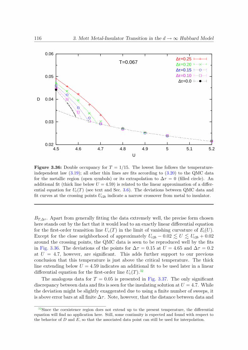
116 3. Mott Metal-Insulator Transition in the d→∞ Hubbard Model
0.02
0.03
0.04
0.05
0.06
4.5 4.6 4.7 4.8 4.9 5 5.1 5.2
D
U
T=0.067∆τ=0.25∆τ=0.20∆τ=0.15∆τ=0.10
∆τ=0.0
Figure 3.36: Double occupancy for T = 1/15. The lowest line follows the temperature-independent law (3.19); all other thin lines are fits according to (3.20) to the QMC datafor the metallic region (open symbols) or its extrapolation to ∆τ = 0 (filled circle). Anadditional fit (thick line below U = 4.59) is related to the linear approximation of a differ-ential equation for Uc(T ) (see text and Sec. 3.6). The deviations between QMC data andfit curves at the crossing points Uc2b indicate a narrow crossover from metal to insulator.
BT,∆τ . Apart from generally fitting the data extremely well, the precise form chosenhere stands out by the fact that it would lead to an exactly linear differential equationfor the first-order transition line Uc(T ) in the limit of vanishing curvature of Ei(U).Except for the close neighborhood of approximately Uc2b − 0.02 . U . Uc2b + 0.02around the crossing points, the QMC data is seen to be reproduced well by the fitsin Fig. 3.36. The deviations of the points for ∆τ = 0.15 at U = 4.65 and ∆τ = 0.2at U = 4.7, however, are significant. This adds further support to our previousconclusion that this temperature is just above the critical temperature. The thickline extending below U = 4.59 indicates an additional fit to be used later in a lineardifferential equation for the first-order line Uc(T ).32
The analogous data for T = 0.05 is presented in Fig. 3.37. The only significantdiscrepancy between data and fits is seen for the insulating solution at U = 4.7. Whilethe deviation might be slightly exaggerated due to using a finite number of sweeps, itis above error bars at all finite ∆τ . Note, however, that the distance between data and
32Since the coexistence region does not extend up to the present temperature, the differentialequation will find no application here. Still, some continuity is expected and found with respect tothe behavior of D and E, so that the associated data point can still be used for interpolation.
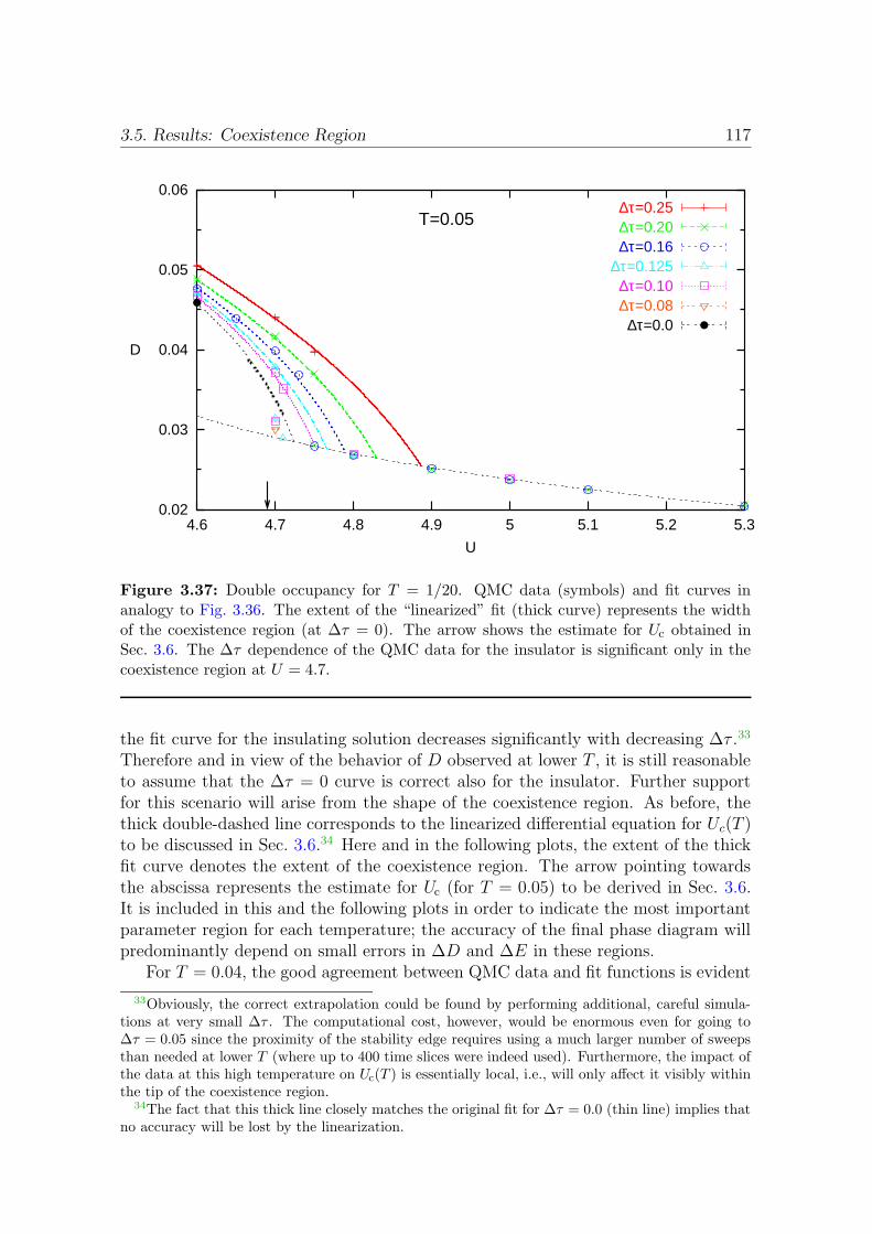
3.5. Results: Coexistence Region 117
0.02
0.03
0.04
0.05
0.06
4.6 4.7 4.8 4.9 5 5.1 5.2 5.3
D
U
T=0.05∆τ=0.25∆τ=0.20∆τ=0.16
∆τ=0.125∆τ=0.10∆τ=0.08
∆τ=0.0
Figure 3.37: Double occupancy for T = 1/20. QMC data (symbols) and fit curves inanalogy to Fig. 3.36. The extent of the “linearized” fit (thick curve) represents the widthof the coexistence region (at ∆τ = 0). The arrow shows the estimate for Uc obtained inSec. 3.6. The ∆τ dependence of the QMC data for the insulator is significant only in thecoexistence region at U = 4.7.
the fit curve for the insulating solution decreases significantly with decreasing ∆τ .33
Therefore and in view of the behavior of D observed at lower T , it is still reasonableto assume that the ∆τ = 0 curve is correct also for the insulator. Further supportfor this scenario will arise from the shape of the coexistence region. As before, thethick double-dashed line corresponds to the linearized differential equation for Uc(T )to be discussed in Sec. 3.6.34 Here and in the following plots, the extent of the thickfit curve denotes the extent of the coexistence region. The arrow pointing towardsthe abscissa represents the estimate for Uc (for T = 0.05) to be derived in Sec. 3.6.It is included in this and the following plots in order to indicate the most importantparameter region for each temperature; the accuracy of the final phase diagram willpredominantly depend on small errors in ∆D and ∆E in these regions.
For T = 0.04, the good agreement between QMC data and fit functions is evident
33Obviously, the correct extrapolation could be found by performing additional, careful simula-tions at very small ∆τ . The computational cost, however, would be enormous even for going to∆τ = 0.05 since the proximity of the stability edge requires using a much larger number of sweepsthan needed at lower T (where up to 400 time slices were indeed used). Furthermore, the impact ofthe data at this high temperature on Uc(T ) is essentially local, i.e., will only affect it visibly withinthe tip of the coexistence region.
34The fact that this thick line closely matches the original fit for ∆τ = 0.0 (thin line) implies thatno accuracy will be lost by the linearization.
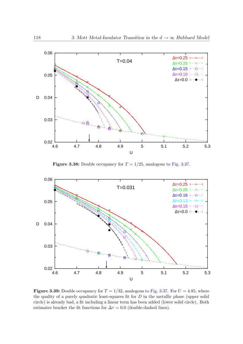
118 3. Mott Metal-Insulator Transition in the d→∞ Hubbard Model
0.02
0.03
0.04
0.05
0.06
4.6 4.7 4.8 4.9 5 5.1 5.2 5.3
D
U
T=0.04∆τ=0.25∆τ=0.20∆τ=0.15∆τ=0.10
∆τ=0.0
Figure 3.38: Double occupancy for T = 1/25, analogous to Fig. 3.37.
0.02
0.03
0.04
0.05
0.06
4.6 4.7 4.8 4.9 5 5.1 5.2 5.3
D
U
T=0.031∆τ=0.25∆τ=0.20∆τ=0.16∆τ=0.13∆τ=0.10
∆τ=0.0
Figure 3.39: Double occupancy for T = 1/32, analogous to Fig. 3.37. For U = 4.85, wherethe quality of a purely quadratic least-squares fit for D in the metallic phase (upper solidcircle) is already bad, a fit including a linear term has been added (lower solid circle). Bothestimates bracket the fit functions for ∆τ = 0.0 (double-dashed lines).
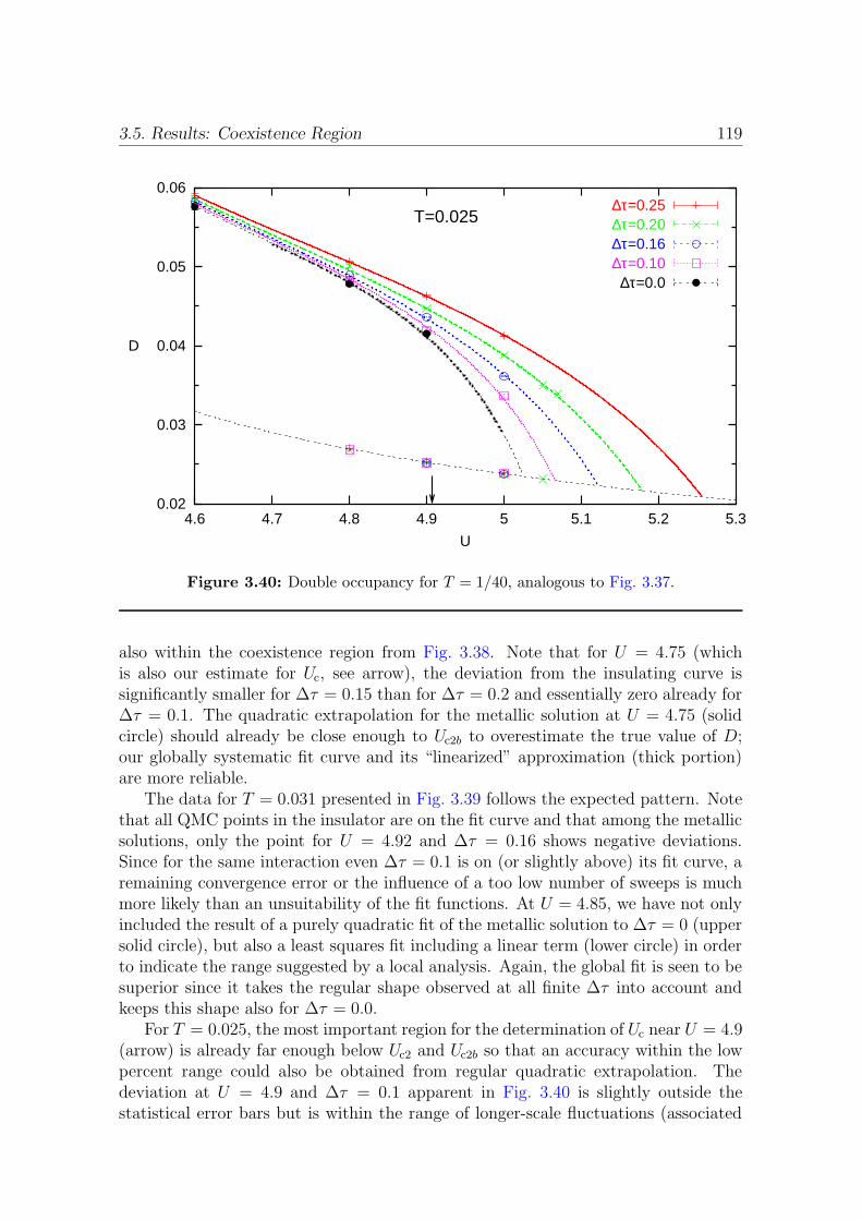
3.5. Results: Coexistence Region 119
0.02
0.03
0.04
0.05
0.06
4.6 4.7 4.8 4.9 5 5.1 5.2 5.3
D
U
T=0.025∆τ=0.25∆τ=0.20∆τ=0.16∆τ=0.10
∆τ=0.0
Figure 3.40: Double occupancy for T = 1/40, analogous to Fig. 3.37.
also within the coexistence region from Fig. 3.38. Note that for U = 4.75 (whichis also our estimate for Uc, see arrow), the deviation from the insulating curve issignificantly smaller for ∆τ = 0.15 than for ∆τ = 0.2 and essentially zero already for∆τ = 0.1. The quadratic extrapolation for the metallic solution at U = 4.75 (solidcircle) should already be close enough to Uc2b to overestimate the true value of D;our globally systematic fit curve and its “linearized” approximation (thick portion)are more reliable.
The data for T = 0.031 presented in Fig. 3.39 follows the expected pattern. Notethat all QMC points in the insulator are on the fit curve and that among the metallicsolutions, only the point for U = 4.92 and ∆τ = 0.16 shows negative deviations.Since for the same interaction even ∆τ = 0.1 is on (or slightly above) its fit curve, aremaining convergence error or the influence of a too low number of sweeps is muchmore likely than an unsuitability of the fit functions. At U = 4.85, we have not onlyincluded the result of a purely quadratic fit of the metallic solution to ∆τ = 0 (uppersolid circle), but also a least squares fit including a linear term (lower circle) in orderto indicate the range suggested by a local analysis. Again, the global fit is seen to besuperior since it takes the regular shape observed at all finite ∆τ into account andkeeps this shape also for ∆τ = 0.0.
For T = 0.025, the most important region for the determination of Uc near U = 4.9(arrow) is already far enough below Uc2 and Uc2b so that an accuracy within the lowpercent range could also be obtained from regular quadratic extrapolation. Thedeviation at U = 4.9 and ∆τ = 0.1 apparent in Fig. 3.40 is slightly outside thestatistical error bars but is within the range of longer-scale fluctuations (associated
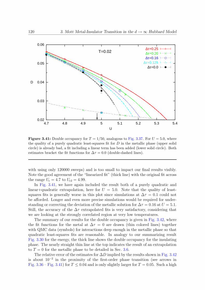
120 3. Mott Metal-Insulator Transition in the d→∞ Hubbard Model
0.02
0.03
0.04
0.05
0.06
4.7 4.8 4.9 5 5.1 5.2 5.3 5.4
D
U
T=0.02∆τ=0.25∆τ=0.20∆τ=0.16
∆τ=0.125∆τ=0.0
Figure 3.41: Double occupancy for T = 1/50, analogous to Fig. 3.37. For U = 5.0, wherethe quality of a purely quadratic least-squares fit for D in the metallic phase (upper solidcircle) is already bad, a fit including a linear term has been added (lower solid circle). Bothestimates bracket the fit functions for ∆τ = 0.0 (double-dashed lines).
with using only 120000 sweeps) and is too small to impact our final results visibly.Note the good agreement of the “linearized fit” (thick line) with the original fit acrossthe range Uc = 4.7 to Uc2 = 4.99.
In Fig. 3.41, we have again included the result both of a purely quadratic andlinear+quadratic extrapolation, here for U = 5.0. Note that the quality of least-squares fits is generally worse in this plot since simulations at ∆τ = 0.1 could notbe afforded. Longer and even more precise simulations would be required for under-standing or correcting the deviation of the metallic solution for ∆τ = 0.16 at U = 5.1.Still, the accuracy of the ∆τ extrapolated fits is very satisfactory, considering thatwe are looking at the strongly correlated region at very low temperatures.
The summary of our results for the double occupancy is given in Fig. 3.42, wherethe fit functions for the metal at ∆τ = 0 are drawn (thin colored lines) togetherwith QMC data (symbols) for interactions deep enough in the metallic phase so thatquadratic least-squares fits are reasonable. In analogy to our summarizing resultFig. 3.30 for the energy, the thick line shows the double occupancy for the insulatingphase. The nearly straight thin line at the top indicates the result of an extrapolationto T = 0 for the metallic phase to be detailed in Sec. 3.6.
The relative error of the estimates for ∆D implied by the results shown in Fig. 3.42is about 10−2 in the proximity of the first-order phase transition (see arrows inFig. 3.36 – Fig. 3.41) for T ≤ 0.04 and is only slightly larger for T = 0.05. Such a high

3.6. Results: Thermodynamic Phase Transition Line 121
0.02
0.03
0.04
0.05
0.06
0.07
4.5 4.6 4.7 4.8 4.9 5 5.1
D
U
metal: T=0.0 (fit)metal: T=0.020metal: T=0.025metal: T=0.031metal: T=0.040metal: T=0.050metal: T=0.067
insulator
Figure 3.42: Double occupancy D vs. interaction U at ∆τ = 0. The symbols indicateextrapolated QMC data for the metallic phase; colored lines indicate “linearized” fit curves(thick lines in Fig. 3.36 – Fig. 3.41). The thick solid line denotes the double occupancy ofthe insulator within its T -dependent stability region. The thin top line marks the groundstate double occupancy in the metal (to be determined in Sec. 3.6).
accuracy may seem surprising in view of our discussion initiated in subsection 3.5.1and continued in the beginning of this subsection. However, the choice of suitable fitfunctions has made it possible to perform a nonlocal ∆τ extrapolation (i.e., for allvalues of U at the same time for fixed T ), including both physical intuition and priorknowledge that had been obtained in subsection 3.5.3. Thus, reliable estimates ofD could be obtained even close to the MIT where naive, local extrapolations wouldhave failed (as illustrated in Fig. 3.34).
3.6 Results: Thermodynamic Phase Transition Line
In this section, a differential equation will be derived for the transition line Uc(T )between metal and insulator based on the fact that both phases have the same freeenergy along the transition line.
3.6.1 Differential Equation for dUc /dT and Linearization
For the Hubbard model, the free energy F and its differential dF can be expressed interms of energy E, temperature T , entropy S, double occupancy D, and interaction

122 3. Mott Metal-Insulator Transition in the d→∞ Hubbard Model
strength U asF = E − TS; dF = −S dT +D dU. (3.21)
These expressions are not directly useful in the context of QMC simulations. Aspointed out in Sec. 1.3, the free energy cannot be estimated using QMC since theimportance sampling technique by construction samples the partition sum only up toan unknown prefactor. Since E can be measured within QMC (and T is an externalparameter), this argument and (3.21) also imply the inability of QMC to measure Sdirectly. However, using
∂βF
∂β
∣∣∣∣U
= F + β∂F
∂β
∣∣∣∣U
= F − T ∂F
∂T
∣∣∣∣U
= F + TS = E (3.22)
with β = 1/T , the differential may be rewritten as
d(βF (β, U)) = E(β, U) dβ + βD(β, U) dU , (3.23)
i.e., expressed in terms of observables which we have determined in Sec. 3.5. Providedthat both the metallic and the insulating solution can be continuously followed (ingeneral on different paths35 in the (U ,β) plane) up to a point (U1,β1) in the crossoverregion where they coincide, then by integrating equation (3.23) one can calculateβFm/i(β, U)− β1F (β1, U1) within the coexistence region and, in principle, determinethe transition line.36 In practice, however, it is likely that along these different pathsdifferent systematic errors will contribute to the free energy estimates for metal andinsulator, respectively. Consequently, the resulting estimate for the transition linemay be systematically biased.
Systematic errors can be kept to a minimum in a scheme where differences inobservables (between metal and insulator) are only computed locally, i.e., for fixedU and β. This may be achieved by rewriting equation (3.23) for metal/insulator
d(βFm/i(β, U)
)= Em/i(β, U) dβ + βDm/i(β, U) dU (3.24)
and taking the difference
d(β∆F (β, U)
)= ∆E(β, U) dβ + β∆D(β, U) dU . (3.25)
Here, ∆F (β, U) = Fm(β, U)− Fi(β, U); corresponding differences for the energy anddouble occupancy are denoted by ∆E and ∆D, respectively. Since the transitionline Uc(β) is smooth and determined by ∆F (β, Uc(β)) = 0, all derivatives of ∆F alsovanish along the line Uc(β). This is true, in particular, for the differential:
d(β∆F (β, U))|U=Uc(β) = 0. (3.26)
From (3.25) and (3.26) we get
0 = ∆E(β, Uc(β)) dβ + β∆D(β, Uc(β)) dUc (3.27)
35The necessity of using different paths for metallic and insulating solutions arises from the shiftof the coexistence region with ∆τ and from the larger numerical errors of each solution near itsstability edge.
36Here and in the following, the indices m and i indicate metal and insulator, respectively.
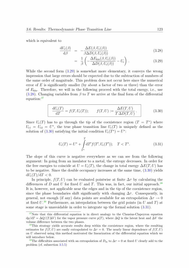
3.6. Results: Thermodynamic Phase Transition Line 123
which is equivalent to
dUc(β)
dβ= − ∆E(β, Uc(β))
β∆D(β, Uc(β))(3.28)
=1
β
(
−∆Ekin(β, Uc(β))
∆D(β, Uc(β))− Uc
)
. (3.29)
While the second form (3.29) is somewhat more elementary, it conveys the wrongimpression that large errors should be expected due to the subtraction of numbers ofthe same order of magnitude. This problem does not occur here since the numericalerror of E is significantly smaller (by about a factor of two or three) than the errorof Ekin. Therefore, we will in the following proceed with the total energy, i.e., use(3.28). Changing variables from β to T we arrive at the final form of the differentialequation:37
dUc(T )
dT= f(T, Uc(T )); f(T, U) :=
∆E(T, U)
T ∆D(T, U). (3.30)
Since Uc(T ) has to go through the tip of the coexistence region (T = T ∗) whereUc1 = Uc2 = U ∗, the true phase transition line Uc(T ) is uniquely defined as thesolution of (3.30) satisfying the initial condition Uc(T
∗) = U ∗:
Uc(T ) = U ∗ +
T∫
T ∗
dT ′f(T ′, Uc(T′)); T < T ∗. (3.31)
The slope of this curve is negative everywhere as we can see from the followingargument: In going from an insulator to a metal, the entropy decreases. In order forthe free energies to coincide at U = Uc(T ), the change in total energy ∆E(T, U) hasto be negative. Since the double occupancy increases at the same time, (3.30) yieldsdUc(T )/dT < 0.
In principle, f(T, U) can be evaluated pointwise at finite ∆τ by calculating thedifferences of D and U for fixed U and T . This was, in fact, our initial approach.38
It is, however, not applicable near the edges and in the tip of the coexistence region,since the phase boundaries shift significantly with changing ∆τ . Consequently, ingeneral, not enough (if any) data points are available for an extrapolation ∆τ → 0at fixed U .39 Furthermore, an interpolation between the grid points (in U and T ) atsome stage is unavoidable in order to integrate up the formal solution (3.31).
37Note that this differential equation is in direct analogy to the Clausius-Clapeyron equationdp/dT = ∆Q/(T∆V ) for the vapor pressure curve p(T ), where ∆Q is the latent heat and ∆V thevolume difference between the two phases.
38This strategy yields accurate results deep within the coexistence region, where the resultingestimates for f(T,U) are easily extrapolated to ∆τ = 0. The nearly linear dependence of f(T,U)on U observed using this method motivated the linearization of the differential equation which wewill introduce below.
39The difficulties associated with an extrapolation of Dm to ∆τ = 0 at fixed U clearly add to theproblem (cf. subsection 3.5.5)

124 3. Mott Metal-Insulator Transition in the d→∞ Hubbard Model
a) b)
-30
-25
-20
-15
-10
-5
0
4.5 4.6 4.7 4.8 4.9 5 5.1
f(T
,U)
U
T=0.067T=0.050T=0.040T=0.031T=0.025T=0.020
-30
-25
-20
-15
-10
-5
0
4.5 4.6 4.7 4.8 4.9 5 5.1
f(T
,U)
U
T=0.067T=0.050T=0.040T=0.031T=0.025T=0.020
Figure 3.43: Function f(T,U) which coincides with the derivative dUc /dT on the phasetransition line Uc(T ). a) “Raw data” extracted from fits of QMC data for E and D.b) Linearized fits with the functional form f(T,U) = A(T )+43U . Circles indicate dUc /dTof the final solution.
Therefore, very accurate results in the whole coexistence region can only beachieved using the fit functions for Ei(U), Di(U), Em(T, U), and Dm(T, U) estab-lished in subsections 3.5.2, 3.5.3, and 3.5.5. Among these data sets, by far the largesterror is associated with the double occupancy Dm(T, U) in the metallic phase. Figure3.43a shows “raw” results for f(T, U) which follow from the QMC data when thebest estimate for Dm according to the 2-parameter fits (3.20) (shown as thin linesin Fig. 3.36 – Fig. 3.41) are used. Here, the fit functions are not only shown within(our estimate of) the coexistence region, but extend up to U = Uc2b(T ) (where theextrapolated energy of the metal crosses the energy of the insulator). Evidently,the dependence on U is almost linear for fixed T . Furthermore, the slope of thecurves shown in Fig. 3.43a is only very weakly dependent on T , at least within thecoexistence region. Consequently, only a small error is made when these raw resultsare replaced by straight lines with identical slopes throughout the coexistence re-gion. This is seen in Fig. 3.43b, where the thick lines (shown only for U within thecoexistence region) follow the form
f(T, U) = A(T ) + 43U . (3.32)
While the discrepancy between this linearized form and the original raw data is inthe percent range throughout the coexistence region, it is even smaller near the mostimportant points touched by the solution (circles) to be determined below. Thisfact alone ensures that the linearized form of f(T, U) is a good interpolation forthe purpose of finding the solution Uc(T ). The particular practical advantage ofthe linear form (3.32) is that the solution of the corresponding differential equationdUc /dT = A(T )+43Uc(T ) is given by a regular integral which can even be performedanalytically using the interpolation for A(T ) that will be established later in thissection.
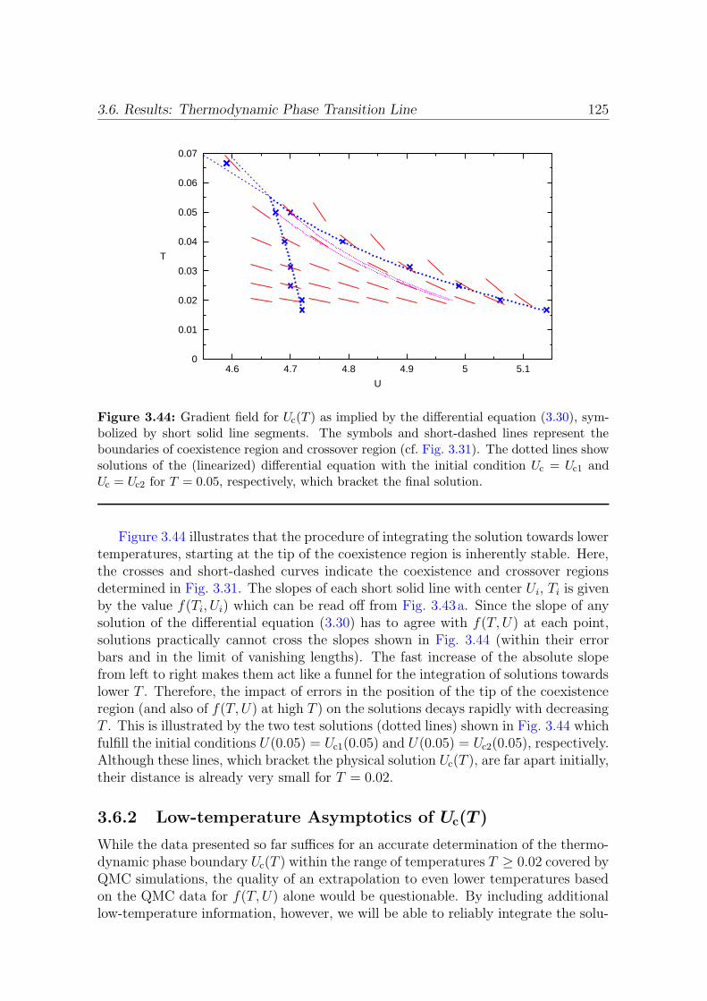
3.6. Results: Thermodynamic Phase Transition Line 125
0
0.01
0.02
0.03
0.04
0.05
0.06
0.07
4.6 4.7 4.8 4.9 5 5.1
T
U
Figure 3.44: Gradient field for Uc(T ) as implied by the differential equation (3.30), sym-bolized by short solid line segments. The symbols and short-dashed lines represent theboundaries of coexistence region and crossover region (cf. Fig. 3.31). The dotted lines showsolutions of the (linearized) differential equation with the initial condition Uc = Uc1 andUc = Uc2 for T = 0.05, respectively, which bracket the final solution.
Figure 3.44 illustrates that the procedure of integrating the solution towards lowertemperatures, starting at the tip of the coexistence region is inherently stable. Here,the crosses and short-dashed curves indicate the coexistence and crossover regionsdetermined in Fig. 3.31. The slopes of each short solid line with center Ui, Ti is givenby the value f(Ti, Ui) which can be read off from Fig. 3.43a. Since the slope of anysolution of the differential equation (3.30) has to agree with f(T, U) at each point,solutions practically cannot cross the slopes shown in Fig. 3.44 (within their errorbars and in the limit of vanishing lengths). The fast increase of the absolute slopefrom left to right makes them act like a funnel for the integration of solutions towardslower T . Therefore, the impact of errors in the position of the tip of the coexistenceregion (and also of f(T, U) at high T ) on the solutions decays rapidly with decreasingT . This is illustrated by the two test solutions (dotted lines) shown in Fig. 3.44 whichfulfill the initial conditions U(0.05) = Uc1(0.05) and U(0.05) = Uc2(0.05), respectively.Although these lines, which bracket the physical solution Uc(T ), are far apart initially,their distance is already very small for T = 0.02.
3.6.2 Low-temperature Asymptotics of Uc(T )
While the data presented so far suffices for an accurate determination of the thermo-dynamic phase boundary Uc(T ) within the range of temperatures T ≥ 0.02 covered byQMC simulations, the quality of an extrapolation to even lower temperatures basedon the QMC data for f(T, U) alone would be questionable. By including additionallow-temperature information, however, we will be able to reliably integrate the solu-

126 3. Mott Metal-Insulator Transition in the d→∞ Hubbard Model
tion down to T = 0. More precisely, we will first derive the asymptotic form of Uc(T )for T → 0 analytically [which implies corresponding asymptotics for f(T, U)] and fixits numerical parameter in a second step using various extrapolated QMC data. Thisprocedure will not only allow for a controlled construction of the full phase diagram,but validate the internal consistency of our results and some underlying assumptionsat the same time.
Consequences of Fermi Liquid Theory
As we have established in subsection 3.5.3, the energy in the (low-temperature) in-sulating phase is independent of the temperature.40 By virtue of (3.21), the sameapplies to the entropy in this phase. In addition, Si is independent of U ; its valueper lattice site equals S0 = ln 2 (Georges et al., 1996; Gebhard, 1997; Kalinowski andGebhard, 2002). Thus, the free energy of the insulator at low T is determined by
Ei(T, U) = E0i (U); Si(T, U) = S0 . (3.33)
Fermi liquid properties imply for the metallic phase that
Em(T, U) = E0m(U) +
1
2γ(U)T 2; Sm(T, U) = γ(U)T , (3.34)
where γ(U) is the linear coefficient of the zero-temperature specific heat. Using theprojective self-consistent technique (PSCT), Moeller established that Uc(0) = Uc2(0),i.e., that the metallic solution is always stable within the coexistence region at T = 0(Moeller et al., 1995; Georges et al., 1996). According to the PSCT, the energydifference between metal and insulator vanishes quadratically for U → U 0
c while thespecific heat diverges,
E0i (U)− E0
m(U) =a
2(U − U 0
c )2; γ(U) =γ0
U0c − U
. (3.35)
Since the PSCT is reliable only for exponents, not for absolute prefactors, a andγ0 should for the moment be regarded as unknown parameters. Equating the freeenergies, we conclude
0 = ∆F (T, Uc) =a
2(U − U 0
c )2 +1
2γ(U)T 2 − TS0, (3.36)
to obtain the low-temperature solution,
Uc(T ) = U 0c −
√
2SoT
a+O(T ) . (3.37)
Consequently, the temperature derivative of the solution has a square root divergenceat low T ,
dUc(T )
dT= −
√
So2aT
+O(1) . (3.38)
40Note that the temperatures under consideration are so small that exponential corrections canbe safely neglected (cf. subsection 3.5.2).
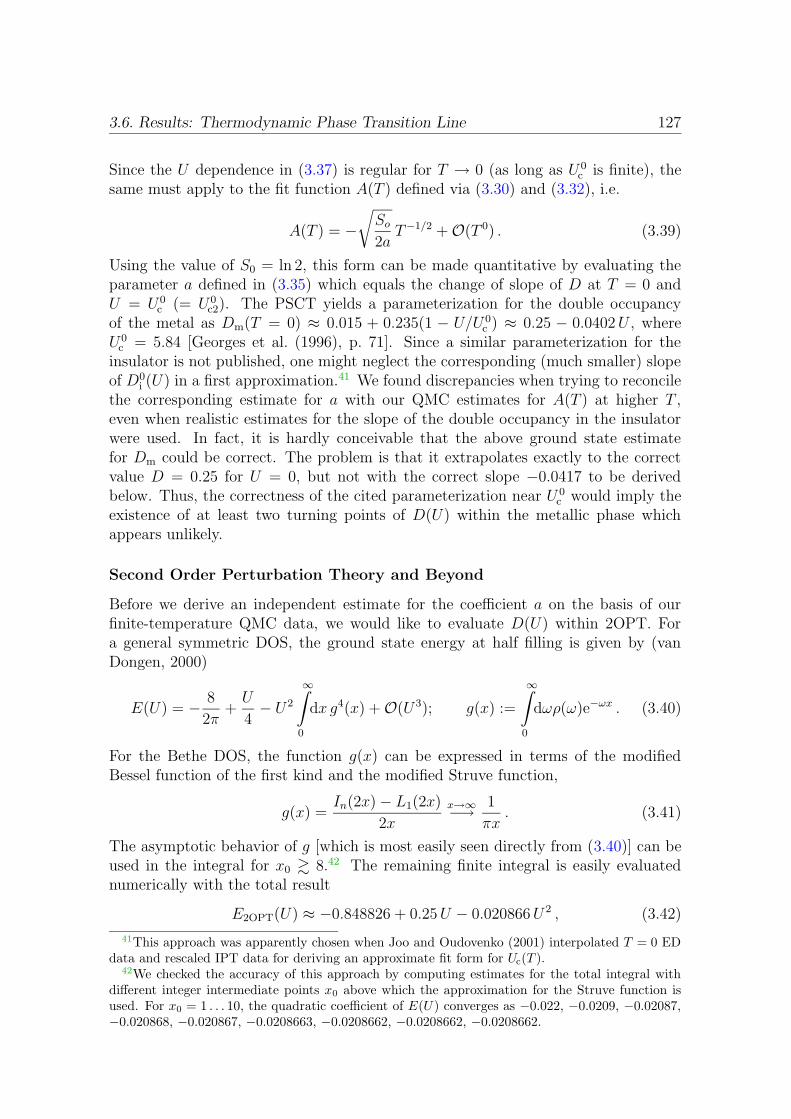
3.6. Results: Thermodynamic Phase Transition Line 127
Since the U dependence in (3.37) is regular for T → 0 (as long as U 0c is finite), the
same must apply to the fit function A(T ) defined via (3.30) and (3.32), i.e.
A(T ) = −√
So2aT−1/2 +O(T 0) . (3.39)
Using the value of S0 = ln 2, this form can be made quantitative by evaluating theparameter a defined in (3.35) which equals the change of slope of D at T = 0 andU = U 0
c (= U 0c2). The PSCT yields a parameterization for the double occupancy
of the metal as Dm(T = 0) ≈ 0.015 + 0.235(1 − U/U 0c ) ≈ 0.25 − 0.0402U , where
U0c = 5.84 [Georges et al. (1996), p. 71]. Since a similar parameterization for the
insulator is not published, one might neglect the corresponding (much smaller) slopeof D0
i (U) in a first approximation.41 We found discrepancies when trying to reconcilethe corresponding estimate for a with our QMC estimates for A(T ) at higher T ,even when realistic estimates for the slope of the double occupancy in the insulatorwere used. In fact, it is hardly conceivable that the above ground state estimatefor Dm could be correct. The problem is that it extrapolates exactly to the correctvalue D = 0.25 for U = 0, but not with the correct slope −0.0417 to be derivedbelow. Thus, the correctness of the cited parameterization near U 0
c would imply theexistence of at least two turning points of D(U) within the metallic phase whichappears unlikely.
Second Order Perturbation Theory and Beyond
Before we derive an independent estimate for the coefficient a on the basis of ourfinite-temperature QMC data, we would like to evaluate D(U) within 2OPT. Fora general symmetric DOS, the ground state energy at half filling is given by (vanDongen, 2000)
E(U) = − 8
2π+U
4− U 2
∞∫
0
dx g4(x) +O(U 3); g(x) :=
∞∫
0
dωρ(ω)e−ωx . (3.40)
For the Bethe DOS, the function g(x) can be expressed in terms of the modifiedBessel function of the first kind and the modified Struve function,
g(x) =In(2x)− L1(2x)
2x
x→∞−→ 1
πx. (3.41)
The asymptotic behavior of g [which is most easily seen directly from (3.40)] can beused in the integral for x0 & 8.42 The remaining finite integral is easily evaluatednumerically with the total result
E2OPT(U) ≈ −0.848826 + 0.25U − 0.020866U 2 , (3.42)
41This approach was apparently chosen when Joo and Oudovenko (2001) interpolated T = 0 EDdata and rescaled IPT data for deriving an approximate fit form for Uc(T ).
42We checked the accuracy of this approach by computing estimates for the total integral withdifferent integer intermediate points x0 above which the approximation for the Struve function isused. For x0 = 1 . . . 10, the quadratic coefficient of E(U) converges as −0.022, −0.0209, −0.02087,−0.020868, −0.020867, −0.0208663, −0.0208662, −0.0208662, −0.0208662.
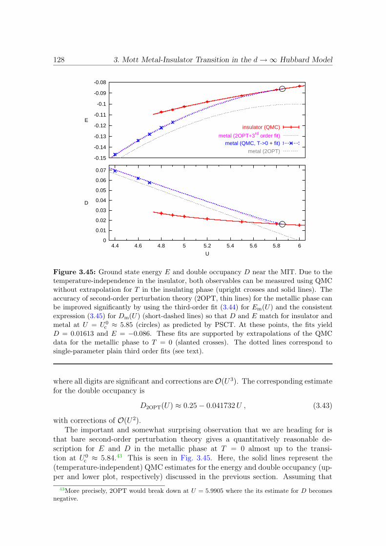
128 3. Mott Metal-Insulator Transition in the d→∞ Hubbard Model
-0.15
-0.14
-0.13
-0.12
-0.11
-0.1
-0.09
-0.08
Einsulator (QMC)
metal (2OPT+3rd order fit)metal (QMC, T->0 + fit)
metal (2OPT)
0
0.01
0.02
0.03
0.04
0.05
0.06
0.07
4.4 4.6 4.8 5 5.2 5.4 5.6 5.8 6
D
U
Figure 3.45: Ground state energy E and double occupancy D near the MIT. Due to thetemperature-independence in the insulator, both observables can be measured using QMCwithout extrapolation for T in the insulating phase (upright crosses and solid lines). Theaccuracy of second-order perturbation theory (2OPT, thin lines) for the metallic phase canbe improved significantly by using the third-order fit (3.44) for Em(U) and the consistentexpression (3.45) for Dm(U) (short-dashed lines) so that D and E match for insulator andmetal at U = U0
c ≈ 5.85 (circles) as predicted by PSCT. At these points, the fits yieldD = 0.01613 and E = −0.086. These fits are supported by extrapolations of the QMCdata for the metallic phase to T = 0 (slanted crosses). The dotted lines correspond tosingle-parameter plain third order fits (see text).
where all digits are significant and corrections areO(U 3). The corresponding estimatefor the double occupancy is
D2OPT(U) ≈ 0.25− 0.041732U , (3.43)
with corrections of O(U 2).The important and somewhat surprising observation that we are heading for is
that bare second-order perturbation theory gives a quantitatively reasonable de-scription for E and D in the metallic phase at T = 0 almost up to the transi-tion at U 0
c ≈ 5.84.43 This is seen in Fig. 3.45. Here, the solid lines represent the(temperature-independent) QMC estimates for the energy and double occupancy (up-per and lower plot, respectively) discussed in the previous section. Assuming that
43More precisely, 2OPT would break down at U = 5.9905 where the its estimate for D becomesnegative.
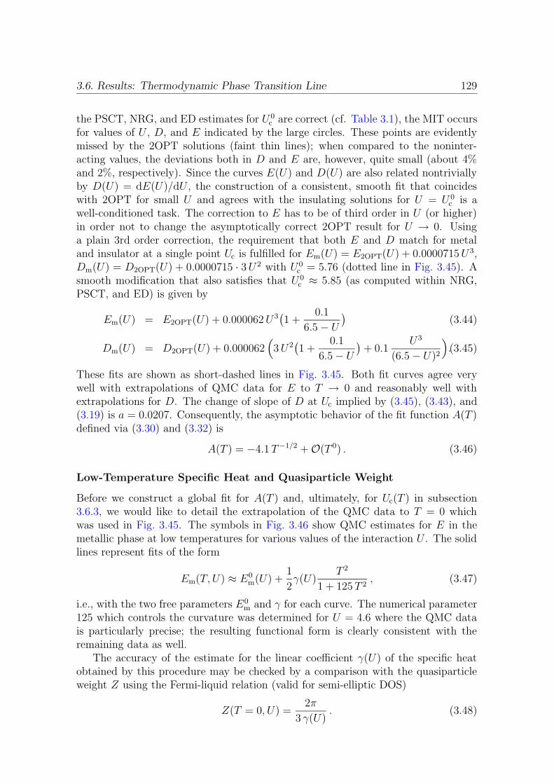
3.6. Results: Thermodynamic Phase Transition Line 129
the PSCT, NRG, and ED estimates for U 0c are correct (cf. Table 3.1), the MIT occurs
for values of U , D, and E indicated by the large circles. These points are evidentlymissed by the 2OPT solutions (faint thin lines); when compared to the noninter-acting values, the deviations both in D and E are, however, quite small (about 4%and 2%, respectively). Since the curves E(U) and D(U) are also related nontriviallyby D(U) = dE(U)/dU , the construction of a consistent, smooth fit that coincideswith 2OPT for small U and agrees with the insulating solutions for U = U 0
c is awell-conditioned task. The correction to E has to be of third order in U (or higher)in order not to change the asymptotically correct 2OPT result for U → 0. Usinga plain 3rd order correction, the requirement that both E and D match for metaland insulator at a single point Uc is fulfilled for Em(U) = E2OPT(U) + 0.0000715U 3,Dm(U) = D2OPT(U) + 0.0000715 · 3U 2 with U 0
c = 5.76 (dotted line in Fig. 3.45). Asmooth modification that also satisfies that U 0
c ≈ 5.85 (as computed within NRG,PSCT, and ED) is given by
Em(U) = E2OPT(U) + 0.000062U 3(1 +
0.1
6.5− U)
(3.44)
Dm(U) = D2OPT(U) + 0.000062(
3U2(1 +
0.1
6.5− U)
+ 0.1U3
(6.5− U)2
)
.(3.45)
These fits are shown as short-dashed lines in Fig. 3.45. Both fit curves agree verywell with extrapolations of QMC data for E to T → 0 and reasonably well withextrapolations for D. The change of slope of D at Uc implied by (3.45), (3.43), and(3.19) is a = 0.0207. Consequently, the asymptotic behavior of the fit function A(T )defined via (3.30) and (3.32) is
A(T ) = −4.1T−1/2 +O(T 0) . (3.46)
Low-Temperature Specific Heat and Quasiparticle Weight
Before we construct a global fit for A(T ) and, ultimately, for Uc(T ) in subsection3.6.3, we would like to detail the extrapolation of the QMC data to T = 0 whichwas used in Fig. 3.45. The symbols in Fig. 3.46 show QMC estimates for E in themetallic phase at low temperatures for various values of the interaction U . The solidlines represent fits of the form
Em(T, U) ≈ E0m(U) +
1
2γ(U)
T 2
1 + 125T 2, (3.47)
i.e., with the two free parameters E0m and γ for each curve. The numerical parameter
125 which controls the curvature was determined for U = 4.6 where the QMC datais particularly precise; the resulting functional form is clearly consistent with theremaining data as well.
The accuracy of the estimate for the linear coefficient γ(U) of the specific heatobtained by this procedure may be checked by a comparison with the quasiparticleweight Z using the Fermi-liquid relation (valid for semi-elliptic DOS)
Z(T = 0, U) =2π
3 γ(U). (3.48)
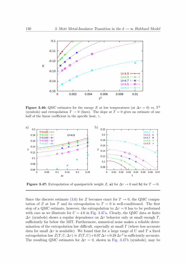
130 3. Mott Metal-Insulator Transition in the d→∞ Hubbard Model
-0.15
-0.14
-0.13
-0.12
-0.11
-0.1
0 0.002 0.004 0.006 0.008 0.01
E
T2
U=4.9U=4.8U=4.7U=4.6U=4.4
Figure 3.46: QMC estimates for the energy E at low temperatures (at ∆τ = 0) vs. T 2
(symbols) and extrapolation T → 0 (lines). The slope at T = 0 gives an estimate of onehalf of the linear coefficient in the specific heat, γ.
a) b)
0.06
0.08
0.1
0.12
0.14
0.16
0.18
0.2
0 0.05 0.1 0.15 0.2 0.25
Z
∆τ
U=4.6T=0.025T=0.031T=0.040T=0.050T=0.067
0.08
0.1
0.12
0.14
0.16
0.18
0.2
0.22
0 0.01 0.02 0.03 0.04 0.05 0.06 0.07
Z
T
U=4.4U=4.6U=4.7U=4.8U=4.9
Figure 3.47: Extrapolation of quasiparticle weight Z, a) for ∆τ → 0 and b) for T → 0.
Since the discrete estimate (3.6) for Z becomes exact for T → 0, the QMC compu-tation of Z at low T and its extrapolation to T = 0 is well-conditioned. The firststep of a QMC estimate, however, the extrapolation to ∆τ = 0 has to be performedwith care as we illustrate for U = 4.6 in Fig. 3.47a. Clearly, the QMC data at finite∆τ (symbols) shows a regular dependence on ∆τ behavior only at small enough T ,sufficiently far below the MIT. Furthermore, numerical noise makes a reliable deter-mination of the extrapolation law difficult, especially at small T (where less accuratedata for small ∆τ is available). We found that for a large range of U and T a fixedextrapolation law Z(T, U,∆τ) ≈ Z(T, U)+0.07 ∆τ+0.28 ∆τ 2 is sufficiently accurate.The resulting QMC estimates for ∆τ = 0, shown in Fig. 3.47b (symbols), may be
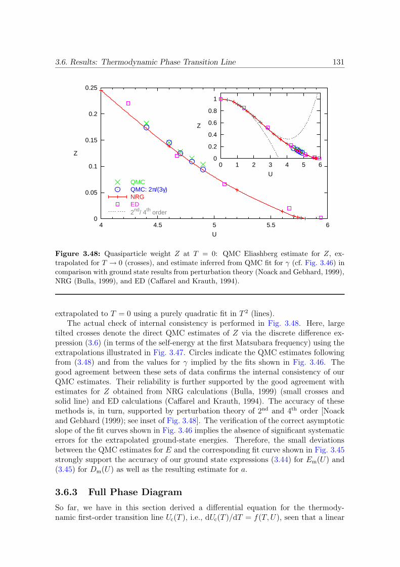
3.6. Results: Thermodynamic Phase Transition Line 131
0
0.05
0.1
0.15
0.2
0.25
4 4.5 5 5.5 6
Z
U
QMCQMC: 2π/(3γ)NRGED2nd/ 4th order
0
0.2
0.4
0.6
0.8
1
0 1 2 3 4 5 6
Z
U
Figure 3.48: Quasiparticle weight Z at T = 0: QMC Eliashberg estimate for Z, ex-trapolated for T → 0 (crosses), and estimate inferred from QMC fit for γ (cf. Fig. 3.46) incomparison with ground state results from perturbation theory (Noack and Gebhard, 1999),NRG (Bulla, 1999), and ED (Caffarel and Krauth, 1994).
extrapolated to T = 0 using a purely quadratic fit in T 2 (lines).The actual check of internal consistency is performed in Fig. 3.48. Here, large
tilted crosses denote the direct QMC estimates of Z via the discrete difference ex-pression (3.6) (in terms of the self-energy at the first Matsubara frequency) using theextrapolations illustrated in Fig. 3.47. Circles indicate the QMC estimates followingfrom (3.48) and from the values for γ implied by the fits shown in Fig. 3.46. Thegood agreement between these sets of data confirms the internal consistency of ourQMC estimates. Their reliability is further supported by the good agreement withestimates for Z obtained from NRG calculations (Bulla, 1999) (small crosses andsolid line) and ED calculations (Caffarel and Krauth, 1994). The accuracy of thesemethods is, in turn, supported by perturbation theory of 2nd and 4th order [Noackand Gebhard (1999); see inset of Fig. 3.48]. The verification of the correct asymptoticslope of the fit curves shown in Fig. 3.46 implies the absence of significant systematicerrors for the extrapolated ground-state energies. Therefore, the small deviationsbetween the QMC estimates for E and the corresponding fit curve shown in Fig. 3.45strongly support the accuracy of our ground state expressions (3.44) for Em(U) and(3.45) for Dm(U) as well as the resulting estimate for a.
3.6.3 Full Phase Diagram
So far, we have in this section derived a differential equation for the thermody-namic first-order transition line Uc(T ), i.e., dUc(T )/dT = f(T, U), seen that a linear
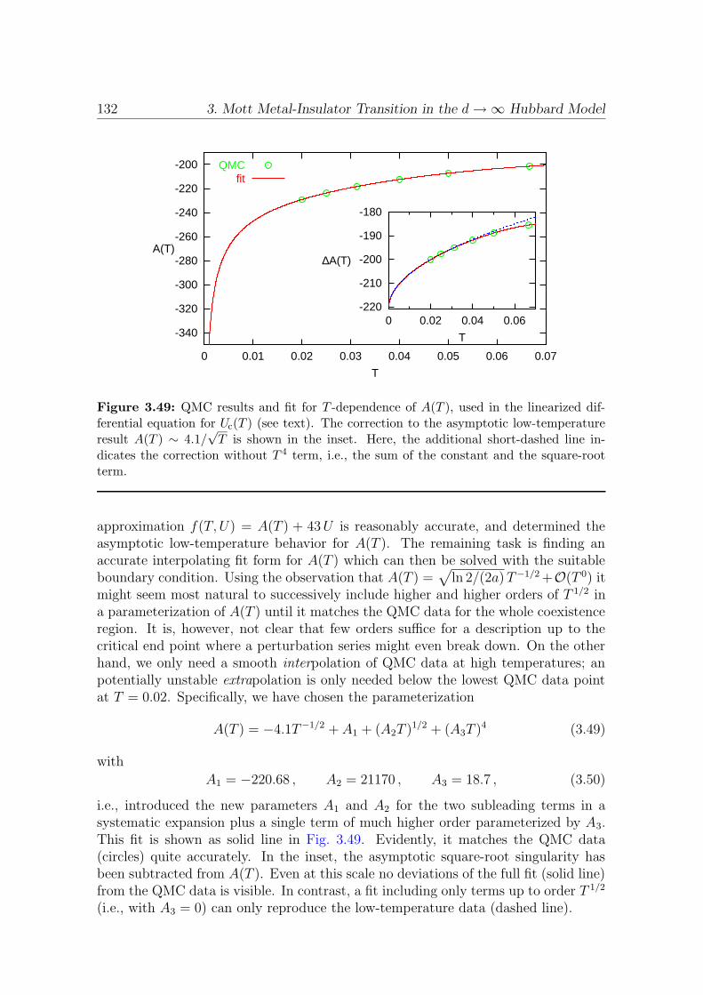
132 3. Mott Metal-Insulator Transition in the d→∞ Hubbard Model
-340
-320
-300
-280
-260
-240
-220
-200
0 0.01 0.02 0.03 0.04 0.05 0.06 0.07
A(T)
T
QMCfit
-220
-210
-200
-190
-180
0 0.02 0.04 0.06
∆A(T)
T
Figure 3.49: QMC results and fit for T -dependence of A(T ), used in the linearized dif-ferential equation for Uc(T ) (see text). The correction to the asymptotic low-temperatureresult A(T ) ∼ 4.1/
√T is shown in the inset. Here, the additional short-dashed line in-
dicates the correction without T 4 term, i.e., the sum of the constant and the square-rootterm.
approximation f(T, U) = A(T ) + 43U is reasonably accurate, and determined theasymptotic low-temperature behavior for A(T ). The remaining task is finding anaccurate interpolating fit form for A(T ) which can then be solved with the suitableboundary condition. Using the observation that A(T ) =
√
ln 2/(2a)T−1/2 +O(T 0) itmight seem most natural to successively include higher and higher orders of T 1/2 ina parameterization of A(T ) until it matches the QMC data for the whole coexistenceregion. It is, however, not clear that few orders suffice for a description up to thecritical end point where a perturbation series might even break down. On the otherhand, we only need a smooth interpolation of QMC data at high temperatures; anpotentially unstable extrapolation is only needed below the lowest QMC data pointat T = 0.02. Specifically, we have chosen the parameterization
A(T ) = −4.1T−1/2 + A1 + (A2T )1/2 + (A3T )4 (3.49)
with
A1 = −220.68 , A2 = 21170 , A3 = 18.7 , (3.50)
i.e., introduced the new parameters A1 and A2 for the two subleading terms in asystematic expansion plus a single term of much higher order parameterized by A3.This fit is shown as solid line in Fig. 3.49. Evidently, it matches the QMC data(circles) quite accurately. In the inset, the asymptotic square-root singularity hasbeen subtracted from A(T ). Even at this scale no deviations of the full fit (solid line)from the QMC data is visible. In contrast, a fit including only terms up to order T 1/2
(i.e., with A3 = 0) can only reproduce the low-temperature data (dashed line).
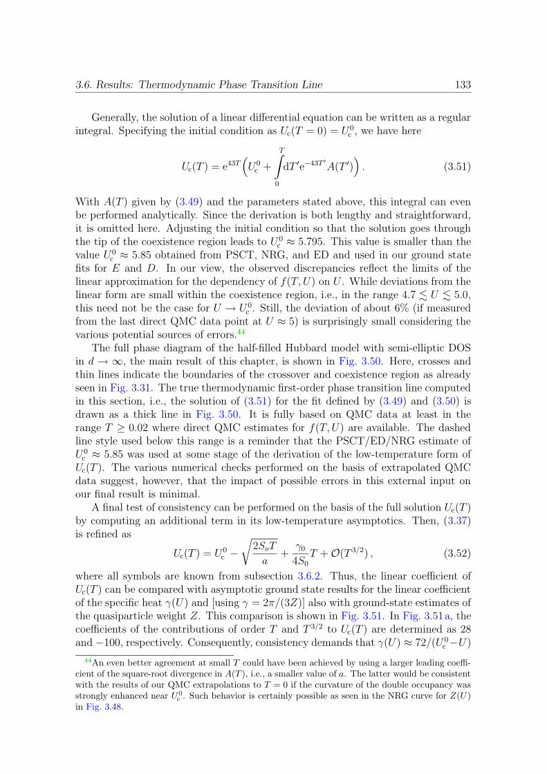
3.6. Results: Thermodynamic Phase Transition Line 133
Generally, the solution of a linear differential equation can be written as a regularintegral. Specifying the initial condition as Uc(T = 0) = U 0
c , we have here
Uc(T ) = e43T(
U0c +
T∫
0
dT ′e−43T ′
A(T ′))
. (3.51)
With A(T ) given by (3.49) and the parameters stated above, this integral can evenbe performed analytically. Since the derivation is both lengthy and straightforward,it is omitted here. Adjusting the initial condition so that the solution goes throughthe tip of the coexistence region leads to U 0
c ≈ 5.795. This value is smaller than thevalue U 0
c ≈ 5.85 obtained from PSCT, NRG, and ED and used in our ground statefits for E and D. In our view, the observed discrepancies reflect the limits of thelinear approximation for the dependency of f(T, U) on U . While deviations from thelinear form are small within the coexistence region, i.e., in the range 4.7 . U . 5.0,this need not be the case for U → U 0
c . Still, the deviation of about 6% (if measuredfrom the last direct QMC data point at U ≈ 5) is surprisingly small considering thevarious potential sources of errors.44
The full phase diagram of the half-filled Hubbard model with semi-elliptic DOSin d → ∞, the main result of this chapter, is shown in Fig. 3.50. Here, crosses andthin lines indicate the boundaries of the crossover and coexistence region as alreadyseen in Fig. 3.31. The true thermodynamic first-order phase transition line computedin this section, i.e., the solution of (3.51) for the fit defined by (3.49) and (3.50) isdrawn as a thick line in Fig. 3.50. It is fully based on QMC data at least in therange T ≥ 0.02 where direct QMC estimates for f(T, U) are available. The dashedline style used below this range is a reminder that the PSCT/ED/NRG estimate ofU0
c ≈ 5.85 was used at some stage of the derivation of the low-temperature form ofUc(T ). The various numerical checks performed on the basis of extrapolated QMCdata suggest, however, that the impact of possible errors in this external input onour final result is minimal.
A final test of consistency can be performed on the basis of the full solution Uc(T )by computing an additional term in its low-temperature asymptotics. Then, (3.37)is refined as
Uc(T ) = U 0c −
√
2SoT
a+
γ0
4S0
T +O(T 3/2) , (3.52)
where all symbols are known from subsection 3.6.2. Thus, the linear coefficient ofUc(T ) can be compared with asymptotic ground state results for the linear coefficientof the specific heat γ(U) and [using γ = 2π/(3Z)] also with ground-state estimates ofthe quasiparticle weight Z. This comparison is shown in Fig. 3.51. In Fig. 3.51a, thecoefficients of the contributions of order T and T 3/2 to Uc(T ) are determined as 28and −100, respectively. Consequently, consistency demands that γ(U) ≈ 72/(U 0
c −U)
44An even better agreement at small T could have been achieved by using a larger leading coeffi-cient of the square-root divergence in A(T ), i.e., a smaller value of a. The latter would be consistentwith the results of our QMC extrapolations to T = 0 if the curvature of the double occupancy wasstrongly enhanced near U 0
c . Such behavior is certainly possible as seen in the NRG curve for Z(U)in Fig. 3.48.
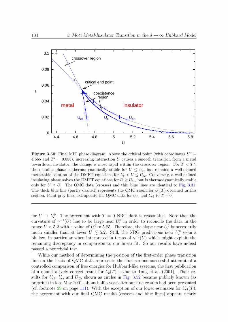
134 3. Mott Metal-Insulator Transition in the d→∞ Hubbard Model
0
0.02
0.04
0.06
0.08
0.1
4.4 4.6 4.8 5 5.2 5.4 5.6 5.8
T
U
metal insulator
crossover region
critical end point
coexistenceregion
Uc1 Uc Uc2
Figure 3.50: Final MIT phase diagram: Above the critical point (with coordinates U ∗ =4.665 and T ∗ = 0.055), increasing interaction U causes a smooth transition from a metaltowards an insulator; the change is most rapid within the crossover region. For T < T ∗,the metallic phase is thermodynamically stable for U ≤ Uc, but remains a well-definedmetastable solution of the DMFT equations for Uc < U ≤ Uc2. Conversely, a well-definedinsulating phase solves the DMFT equations for U ≥ Uc1, but is thermodynamically stableonly for U ≥ Uc. The QMC data (crosses) and thin blue lines are identical to Fig. 3.31.The thick blue line (partly dashed) represents the QMC result for Uc(T ) obtained in thissection. Faint grey lines extrapolate the QMC data for Uc1 and Uc2 to T = 0.
for U → U 0c . The agreement with T = 0 NRG data is reasonable. Note that the
curvature of γ−1(U) has to be large near U 0c in order to reconcile the data in the
range U < 5.2 with a value of U 0c ≈ 5.85. Therefore, the slope near U 0
c is necessarilymuch smaller than at lower U . 5.2. Still, the NRG predictions near U 0
c seem abit low, in particular when interpreted in terms of γ−1(U) which might explain theremaining discrepancy in comparison to our linear fit. So our results have indeedpassed a nontrivial test.
While our method of determining the position of the first-order phase transitionline on the basis of QMC data represents the first serious successful attempt of acontrolled comparison of free energies for Hubbard-like systems, the first publicationof a quantitatively correct result for Uc(T ) is due to Tong et al. (2001). Their re-sults for Uc1, Uc, and Uc2, shown as circles in Fig. 3.52 became publicly known (aspreprint) in late May 2001, about half a year after our first results had been presented(cf. footnote 29 on page 111). With the exception of our lower estimates for Uc1(T ),the agreement with our final QMC results (crosses and blue lines) appears nearly
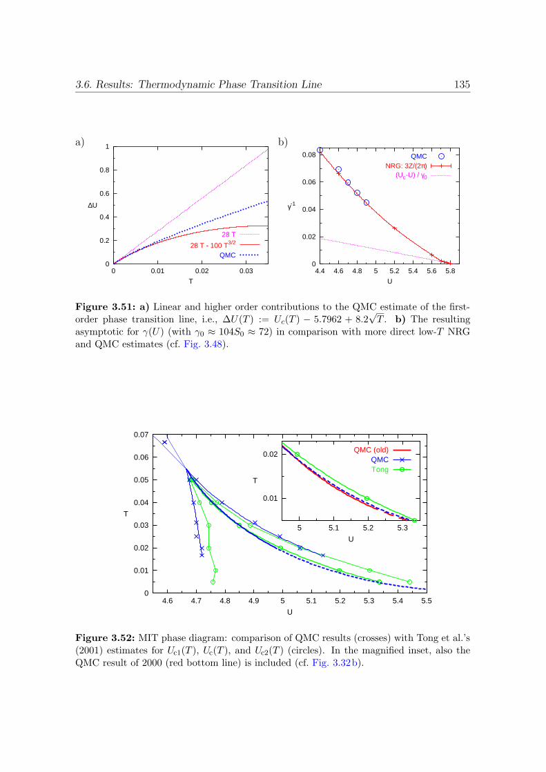
3.6. Results: Thermodynamic Phase Transition Line 135
a) b)
0
0.2
0.4
0.6
0.8
1
0 0.01 0.02 0.03
∆U
T
28 T
28 T - 100 T3/2
QMC0
0.02
0.04
0.06
0.08
4.4 4.6 4.8 5 5.2 5.4 5.6 5.8
γ-1
U
QMCNRG: 3Z/(2π)
(Uc-U) / γ0
Figure 3.51: a) Linear and higher order contributions to the QMC estimate of the first-order phase transition line, i.e., ∆U(T ) := Uc(T ) − 5.7962 + 8.2
√T . b) The resulting
asymptotic for γ(U) (with γ0 ≈ 104S0 ≈ 72) in comparison with more direct low-T NRGand QMC estimates (cf. Fig. 3.48).
0
0.01
0.02
0.03
0.04
0.05
0.06
0.07
4.6 4.7 4.8 4.9 5 5.1 5.2 5.3 5.4 5.5
T
U
0.01
0.02
5 5.1 5.2 5.3
T
U
QMC (old)QMCTong
Figure 3.52: MIT phase diagram: comparison of QMC results (crosses) with Tong et al.’s(2001) estimates for Uc1(T ), Uc(T ), and Uc2(T ) (circles). In the magnified inset, also theQMC result of 2000 (red bottom line) is included (cf. Fig. 3.32b).
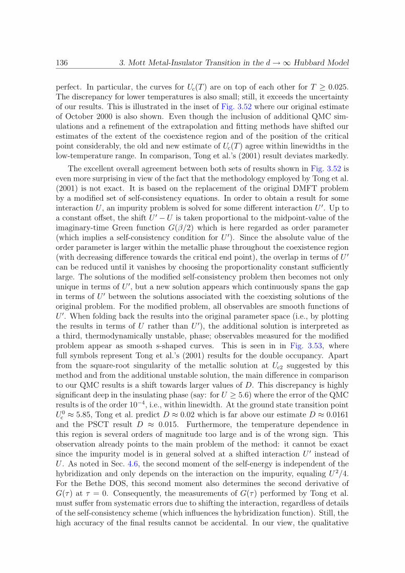
136 3. Mott Metal-Insulator Transition in the d→∞ Hubbard Model
perfect. In particular, the curves for Uc(T ) are on top of each other for T ≥ 0.025.The discrepancy for lower temperatures is also small; still, it exceeds the uncertaintyof our results. This is illustrated in the inset of Fig. 3.52 where our original estimateof October 2000 is also shown. Even though the inclusion of additional QMC sim-ulations and a refinement of the extrapolation and fitting methods have shifted ourestimates of the extent of the coexistence region and of the position of the criticalpoint considerably, the old and new estimate of Uc(T ) agree within linewidths in thelow-temperature range. In comparison, Tong et al.’s (2001) result deviates markedly.
The excellent overall agreement between both sets of results shown in Fig. 3.52 iseven more surprising in view of the fact that the methodology employed by Tong et al.(2001) is not exact. It is based on the replacement of the original DMFT problemby a modified set of self-consistency equations. In order to obtain a result for someinteraction U , an impurity problem is solved for some different interaction U ′. Up toa constant offset, the shift U ′ −U is taken proportional to the midpoint-value of theimaginary-time Green function G(β/2) which is here regarded as order parameter(which implies a self-consistency condition for U ′). Since the absolute value of theorder parameter is larger within the metallic phase throughout the coexistence region(with decreasing difference towards the critical end point), the overlap in terms of U ′
can be reduced until it vanishes by choosing the proportionality constant sufficientlylarge. The solutions of the modified self-consistency problem then becomes not onlyunique in terms of U ′, but a new solution appears which continuously spans the gapin terms of U ′ between the solutions associated with the coexisting solutions of theoriginal problem. For the modified problem, all observables are smooth functions ofU ′. When folding back the results into the original parameter space (i.e., by plottingthe results in terms of U rather than U ′), the additional solution is interpreted asa third, thermodynamically unstable, phase; observables measured for the modifiedproblem appear as smooth s-shaped curves. This is seen in in Fig. 3.53, wherefull symbols represent Tong et al.’s (2001) results for the double occupancy. Apartfrom the square-root singularity of the metallic solution at Uc2 suggested by thismethod and from the additional unstable solution, the main difference in comparisonto our QMC results is a shift towards larger values of D. This discrepancy is highlysignificant deep in the insulating phase (say: for U ≥ 5.6) where the error of the QMCresults is of the order 10−4, i.e., within linewidth. At the ground state transition pointU0
c ≈ 5.85, Tong et al. predict D ≈ 0.02 which is far above our estimate D ≈ 0.0161and the PSCT result D ≈ 0.015. Furthermore, the temperature dependence inthis region is several orders of magnitude too large and is of the wrong sign. Thisobservation already points to the main problem of the method: it cannot be exactsince the impurity model is in general solved at a shifted interaction U ′ instead ofU . As noted in Sec. 4.6, the second moment of the self-energy is independent of thehybridization and only depends on the interaction on the impurity, equaling U 2/4.For the Bethe DOS, this second moment also determines the second derivative ofG(τ) at τ = 0. Consequently, the measurements of G(τ) performed by Tong et al.must suffer from systematic errors due to shifting the interaction, regardless of detailsof the self-consistency scheme (which influences the hybridization function). Still, thehigh accuracy of the final results cannot be accidental. In our view, the qualitative
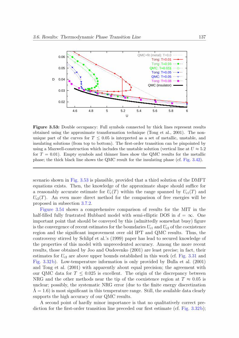
3.6. Results: Thermodynamic Phase Transition Line 137
0.02
0.03
0.04
0.05
0.06
4.6 4.8 5 5.2 5.4 5.6 5.8 6
D
U
QMC+fit (metal): T=0.0Tong: T=0.01Tong: T=0.03
QMC: T=0.031Tong: T=0.05QMC: T=0.05Tong: T=0.08
QMC (insulator)
Figure 3.53: Double occupancy: Full symbols connected by thick lines represent resultsobtained using the approximate transformation technique (Tong et al., 2001). The non-unique part of the curves for T ≤ 0.05 is interpreted as a set of metallic, unstable, andinsulating solutions (from top to bottom). The first-order transition can be pinpointed byusing a Maxwell-construction which includes the unstable solution (vertical line at U ≈ 5.2for T = 0.01). Empty symbols and thinner lines show the QMC results for the metallicphase; the thick black line shows the QMC result for the insulating phase (cf. Fig. 3.42).
scenario shown in Fig. 3.53 is plausible, provided that a third solution of the DMFTequations exists. Then, the knowledge of the approximate shape should suffice fora reasonably accurate estimate for Uc(T ) within the range spanned by Uc1(T ) andUc2(T ). An even more direct method for the comparison of free energies will beproposed in subsection 3.7.2.
Figure 3.54 shows a comprehensive comparison of results for the MIT in thehalf-filled fully frustrated Hubbard model with semi-elliptic DOS in d = ∞. Oneimportant point that should be conveyed by this (admittedly somewhat busy) figureis the convergence of recent estimates for the boundaries Uc1 and Uc2 of the coexistenceregion and the significant improvement over old IPT and QMC results. Thus, thecontroversy stirred by Schlipf et al.’s (1999) paper has lead to secured knowledge ofthe properties of this model with unprecedented accuracy. Among the more recentresults, those obtained by Joo and Oudovenko (2001) are least precise; in fact, theirestimates for Uc2 are above upper bounds established in this work (cf. Fig. 3.31 andFig. 3.32b). Low-temperature information is only provided by Bulla et al. (2001)and Tong et al. (2001) with apparently about equal precision; the agreement withour QMC data for T ≤ 0.025 is excellent. The origin of the discrepancy betweenNRG and the other methods near the tip of the coexistence region at T ≈ 0.05 isunclear; possibly, the systematic NRG error (due to the finite energy discretizationΛ = 1.6) is most significant in this temperature range. Still, the available data clearlysupports the high accuracy of our QMC results.
A second point of hardly minor importance is that no qualitatively correct pre-diction for the first-order transition line preceded our first estimate (cf. Fig. 3.32b);

138 3. Mott Metal-Insulator Transition in the d→∞ Hubbard Model
0
0.02
0.04
0.06
0.08
0.1
4 4.5 5 5.5 6
T
U
crossover regions
RDA
PSCT/ED
metal
insulator
QMC: this workQMC: Joo et al.
NRG: Bulla et al.Trafo/ED: Tong et al.
QMC: Rozenberg et al.IPT: Georges et al.
Figure 3.54: MIT phase diagram: recent finite-temperature results [this work, Joo andOudovenko (2001), Bulla et al. (2001), Tong et al. (2001)] in comparison with formerestimates [Rozenberg et al. (1994), Georges et al. (1996)]. In the low-temperature region,thinner lines represent Uc1 and Uc2. Thick lines show calculated first-order lines Uc(T )[this work, Tong et al., Georges et al.] with the exception of Joo et al.’s estimate [withUc(T ) ≈ Uc2(T ) for T . T ∗] which is based on a rescaling of the IPT curve and a fit toground state data. For ground state data, see Table 3.1; subsets of the finite-T data areshown in Fig. 3.7b, Fig. 3.9, Fig. 3.32b, Fig. 3.33, Fig. 3.50, and Fig. 3.52. For Rozenberget al.’s (1999) QMC results on coexisting phases (not shown here), see Fig. 3.32a andFig. 3.33.
since Tong et al.’s method is approximate (see above), our final curve shown inFig. 3.54 is still the only controlled (and even numerically exact) result. In fact,both the original (cf. Fig. 3.7a) and the later IPT estimates wrongly implied thatUc(T ) ≈ Uc1(T ) for T . T ∗. The implication of Joo et al.’s fitting and scaling pro-cedure that Uc(T ) ≈ Uc2(T ) for T . T ∗ is closer to the truth, but still qualitativelyincorrect. Only the recent independent results of this work and by Tong et al. providesignificant insight with regard to the position of Uc(T ).
3.6.4 Implications of Partial Frustration
After having established the MIT scenario in the fully frustrated case (for semi-ellipticDOS), the interesting question arises what the full phase diagram would look like forpartial frustration. In this context, we have to distinguish between frustration atconstant DOS and the more generic case that the introduction of frustrating bonds

3.6. Results: Thermodynamic Phase Transition Line 139
a) b) c) d)
T
U
(U*,T* )
PM PIT
U
paramagnet
antiferromagnetT
U
PM PIT
U
PM PI
AFM AFI
e) f) g) h)
T
U
PM PIT
U
PM PIT
U
PM PIT
U
PM PI
AFM AFI
Figure 3.55: Schematic phase diagrams of models with semi-elliptic DOS and varyingdegrees of frustration. a) fully frustrated case with first-order paramagnetic MIT (thicksolid line) for 0 ≤ T < T ∗. b) weakly frustrated case with second-order magnetic transition(dashed line); no transitions within paramagnetic or within AF phase. c)-h): strongerfrustrated case with Tmax
N < T ∗. c) first-order line ends on smooth Neel curve. d) first-order MIT crosses smooth Neel curve. e) TN higher on metallic side of MIT line; noimplications for AF phase (shaded) intended. f) TN higher on insulating side of MIT line.g) TN higher on insulating side of MIT line; MIT line shifted in intermediate temperatureregion. h) speculative scenario for full phase diagram: a single first-order MIT line extendsfrom (U∗, T ∗) to (0, 0); it agrees with the fully-frustrated line at large T (solid line) anddeviates below (thick short-dashed line). For the partially frustrated model, only scenariosb) and g) (with the possible completion h)) appear likely (see text). The MIT line ofthe fully frustrated model is drawn as faint thin line for comparison where it is does notrepresent a transition.
also leads to an asymmetry of the DOS.
Frustration at constant semi-elliptic DOS
Within the DMFT, the lattice influences properties of homogeneous phases only viaits (noninteracting) DOS. Thus, the thermodynamics of a partially frustrated modelwith semi-elliptic DOS agrees with that of the fully frustrated model considered so farwithin its paramagnetic phase.45 In the following, we will derive the qualitative char-acteristics of the full phase diagram expected for such a model. For sufficiently smallfrustration, the first-order MIT line present in the fully frustrated model (Fig. 3.55a)is completely hidden by the low-temperature AF phase; then, the phase diagramis qualitatively unchanged from the unfrustrated case as shown in Fig. 3.55b. For
45While the claim (Rozenberg et al., 1995) that uniform NNN hopping on the Bethe lattice leavesthe DOS unchanged was contradicted in subsection 2.2.2, fully disordered hopping on the NNNbonds of a Bethe lattice constitutes a realization of such a model with variable disorder.
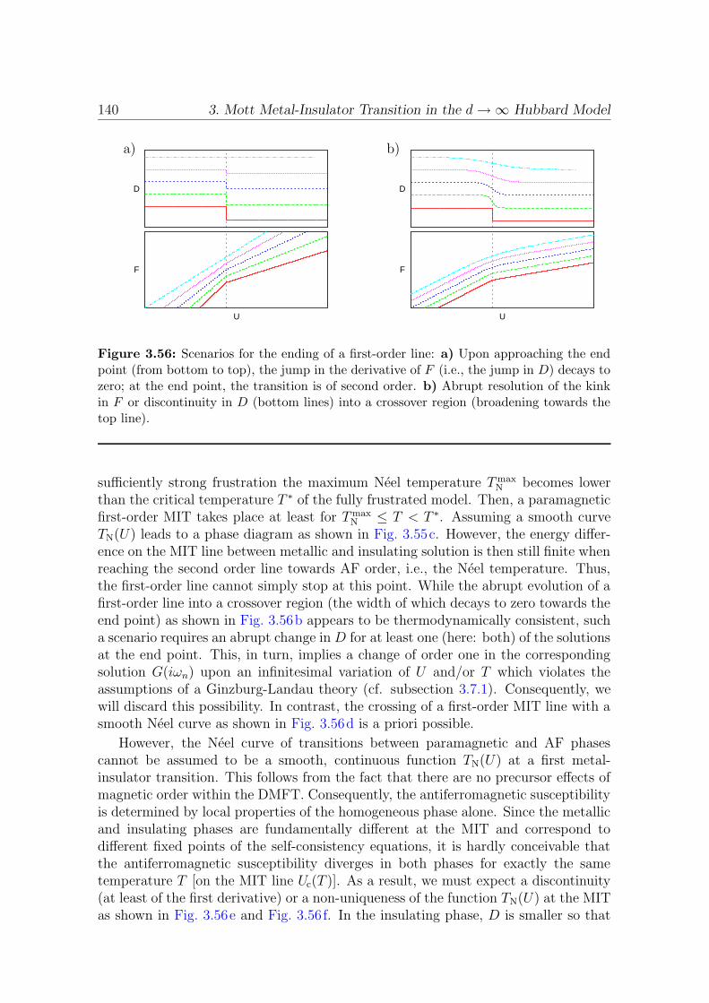
140 3. Mott Metal-Insulator Transition in the d→∞ Hubbard Model
a) b)
F
U
D
F
U
D
Figure 3.56: Scenarios for the ending of a first-order line: a) Upon approaching the endpoint (from bottom to top), the jump in the derivative of F (i.e., the jump in D) decays tozero; at the end point, the transition is of second order. b) Abrupt resolution of the kinkin F or discontinuity in D (bottom lines) into a crossover region (broadening towards thetop line).
sufficiently strong frustration the maximum Neel temperature TmaxN becomes lower
than the critical temperature T ∗ of the fully frustrated model. Then, a paramagneticfirst-order MIT takes place at least for Tmax
N ≤ T < T ∗. Assuming a smooth curveTN(U) leads to a phase diagram as shown in Fig. 3.55c. However, the energy differ-ence on the MIT line between metallic and insulating solution is then still finite whenreaching the second order line towards AF order, i.e., the Neel temperature. Thus,the first-order line cannot simply stop at this point. While the abrupt evolution of afirst-order line into a crossover region (the width of which decays to zero towards theend point) as shown in Fig. 3.56b appears to be thermodynamically consistent, sucha scenario requires an abrupt change in D for at least one (here: both) of the solutionsat the end point. This, in turn, implies a change of order one in the correspondingsolution G(iωn) upon an infinitesimal variation of U and/or T which violates theassumptions of a Ginzburg-Landau theory (cf. subsection 3.7.1). Consequently, wewill discard this possibility. In contrast, the crossing of a first-order MIT line with asmooth Neel curve as shown in Fig. 3.56d is a priori possible.
However, the Neel curve of transitions between paramagnetic and AF phasescannot be assumed to be a smooth, continuous function TN(U) at a first metal-insulator transition. This follows from the fact that there are no precursor effects ofmagnetic order within the DMFT. Consequently, the antiferromagnetic susceptibilityis determined by local properties of the homogeneous phase alone. Since the metallicand insulating phases are fundamentally different at the MIT and correspond todifferent fixed points of the self-consistency equations, it is hardly conceivable thatthe antiferromagnetic susceptibility diverges in both phases for exactly the sametemperature T [on the MIT line Uc(T )]. As a result, we must expect a discontinuity(at least of the first derivative) or a non-uniqueness of the function TN(U) at the MITas shown in Fig. 3.56e and Fig. 3.56f. In the insulating phase, D is smaller so that
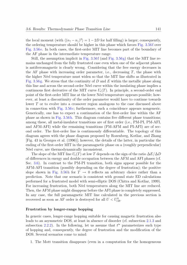
3.6. Results: Thermodynamic Phase Transition Line 141
the local moment (with 〈(n↑−n↓)2〉 = 1− 2D for half filling) is larger; consequently,
the ordering temperature should be higher in this phase which favors Fig. 3.56f overFig. 3.56e. In both cases, the first-order MIT line becomes part of the boundary ofthe AF phase in the intermediate temperature range.
Still, the assumption implicit in Fig. 3.56f (and Fig. 3.56g) that the MIT line re-mains unchanged from the fully frustrated case even when one of the adjacent phasesis antiferromagnetic is clearly wrong. Considering that the free energy decreases inthe AF phase with increasing order parameter, i.e., decreasing T , the phase withthe higher Neel temperature must widen so that the MIT line shifts as illustrated inFig. 3.56g. We stress that the continuity of D and E within the metallic phase alongthis line and across the second-order Neel curve within the insulating phase implies acontinuous first derivative of the MIT curve Uc(T ). In principle, a second-order endpoint of the first-order MIT line at the lower Neel temperature appears possible; how-ever, at least a discontinuity of the order parameter would have to continue towardslower T or to evolve into a crossover region analogous to the case discussed abovein connection with Fig. 3.56c; furthermore, such a coincidence appears nongeneric.Generically, one has to expect a continuation of the first-order line within the AFphase as shown in Fig. 3.56h. This diagram contains five different phase transitions;among these, all metal-insulator transitions are of first order (i.e., PM-PI, PM-AFI,and AFM-AFI) while the remaining transitions (PM-AFM and PI-AFI) are of sec-ond order. The first-order line is continuously differentiable. The topology of thisdiagram agrees with the phase diagram proposed by Rozenberg, Kotliar, and Zhang[Fig. 43 in Georges et al. (1996)]; however, the details of the latter, in particular theending of the first-order MIT in the paramagnetic phase on a (roughly perpendicular)Neel curve, are thermodynamically inconsistent.
The slope of the MIT line Uc(T ) at low T depends on the sign of the ratio ∆E/∆Dof differences in energy and double occupation between the AFM and AFI phases (cf.Sec. 3.6). In contrast to the PM-PI transition, both signs appear possible for theAFM-AFI transition (possibly depending on the degree of frustration); the positiveslope shown in Fig. 3.56h for T → 0 reflects an arbitrary choice rather than aprediction. Note that our scenario is consistent with ground state ED calculationsperformed for a frustrated model with semi-elliptic DOS (Chitra and Kotliar, 1999).For increasing frustration, both Neel temperatures along the MIT line are reduced.Then, the AFM phase might disappear before the AFI phase is completely suppressed.In any case, the full paramagnetic MIT line calculated in the previous section isrecovered as soon as AF order is destroyed for all U < U 0
c2b.
Frustration by longer-range hopping
In generic cases, longer-range hopping suitable for causing magnetic frustration alsoleads to an asymmetric DOS, at least in absence of disorder (cf. subsection 2.1.3 andsubsection 2.2.2). In the following, let us assume that t′∗ parameterizes such typeof hopping and, consequently, the degree of frustration and the modification of theDOS. Several scenarios come to mind:
1. The Mott transition disappears (even in a computation for the homogeneous

142 3. Mott Metal-Insulator Transition in the d→∞ Hubbard Model
a) b) c)
T
U
T
U
T
U
Figure 3.57: Schematic phase diagram for frustration by longer-range hopping. a) In theunfrustrated case, a paramagnetic MIT line (faint thin line) is present only for a calculationrestricted to the paramagnetic phase; in an unrestricted calculation, it is hidden by the low-temperature AF phase (below the Neel curve, dashed). b) and c): Increasing frustrationsuppresses both the AF phase and the MIT line (obtained in a restricted calculation) sothat the latter never becomes thermodynamically relevant.
phase) and a smooth crossover develops for any |t′∗| > 0.
2. The first-order Mott transition survives sufficiently strong finite microscopicfrustration with no or only a minor change of the critical temperature T ∗ sothat TN < T ∗.
3. The Mott transition coexists with NNN hopping, but with T ∗ < TN(U ∗) for allhopping strengths t∗ as illustrated in Fig. 3.57 (with increasing frustration fromleft to right). The MIT line (computed in the enforced homogeneous phase)never reaches the true homogeneous phase.
Since the first suggestion implies changes of order one in solutions of the DMFTequations for an infinitesimal change of the DOS, it may be safely excluded. Thesecond scenario leads to the same conclusions as the case of frustration at constantDOS studied above. The third scenario comprises only a single phase transition line,the Neel curve. In fact, this least interesting possibility seems to apply at least forthe DMFT treatment of the cubic lattice with NNN hopping. Here, T ∗ is stronglysuppressed (from about T ∗ = 1/25 to T ∗ = 1/35) by introducing moderate frustration(t′∗/t∗ = −0.25) according to recent QMC results (Knecht, 2002).
3.7 Landau Theory and Criticality
In this section, we will study some implications of Landau theory. In subsection 3.7.1,we introduce an explicit representation of the lattice contribution to the Ginzburg-Landau free-energy functional for semi-elliptic DOS. Using this formalism, we showthat each step of a direct iteration of the DMFT equations proceeds downhill, i.e.,opposite to the gradient (with respect to the hybridization function) of the free energy.Based on this finding, a new method for evaluating free energy differences betweencoexisting phases within the DMFT is proposed in subsection 3.7.2. In subsection3.7.3, we discuss to which degree critical behavior should impact or become visiblein numerical calculations as performed in this work.
3.7. Landau Theory and Criticality 143
3.7.1 Free Energy Functional for the Bethe Lattice
Within the DMFT, the free energy per particle can in the general homogeneous casebe written as (Georges, Kotliar, and Si, 1992)
F = Fimp − 2T∑
n
[
lnG(iωn) +
∞∫
−∞
dε ρ(ε) ln(iωn + µ− Σ(iωn)− ε
)]
. (3.53)
Here, Fimp is the impurity part corresponding to (1.34). We wish to extract anexplicit expression for the lattice contribution. For the Bethe lattice, we have iωn +µ − Σ(iωn) = t∗2G(iωn) + 1/G(iωn). Therefore, the lattice contribution can beexplicitly written in terms of the Green function Gn ≡ G(iωn). Its derivative reads
− 1
2T
∂
∂Gn
(F −Fimp) =1
Gn
+(
t∗2− 1
G2n
)∞∫
−∞
dε ρ(ε)1
t∗2Gn +G−1n − ε
= t∗2Gn . (3.54)
Consequently, the free energy may be expressed for a semi-elliptic DOS as
F = Fimp − t∗2T∑
n
G2n . (3.55)
For consistency with Kotliar et al. (2000) we continue the discussion in terms of thehybridization function ∆n ≡ ∆(iωn) = iωn + µ− G−1
n . The impurity equation (1.31)is then equivalent (at the self-consistency) to
Gn =1
2T
∂Fimp[T, U,∆]
∂∆n
. (3.56)
Since for the Bethe lattice ∆n = t∗2Gn, the total free energy may also be written asa functional of the hybridization function
F [T, U,∆] = −T∑
n
∆2n
t∗2+ Fimp[T, U,∆] . (3.57)
The important point is that this Ginzburg-Landau functional FGL ≡ F [T, U,∆] isdefined (and real valued) for an arbitrary hybridization function. While the followingconsiderations apply for arbitrary filling, we find it convenient to introduce explicitlyreal-valued notation which is only valid for half filling. Using the short hand notationO′′ ≡ ImO we then have
(∇∆′′F
)
n≡ ∂F [T, U,∆′′]
∂∆′′n
= −2T(G′′n[T, U,∆
′′]− ∆′′n
t∗2
)(3.58)
= −2T(G′′
new(iωn)−G′′old(iωn)
). (3.59)
Here, G′′n[T, U,∆
′′] ≡ G′′new(iωn) denotes the (new) solution of the impurity model for
given ∆′′n/t
∗2 ≡ G′′old(iωn). Eqn. (3.59) implies that each step of a direct iteration
scheme (cf. subsection 3.2.2) advances G exactly opposite to the gradient of F , i.e.,

144 3. Mott Metal-Insulator Transition in the d→∞ Hubbard Model
downhill.46 If ∇∆F changes slowly on the scale of the step length, we can approximatethe change in F by the first term in a Taylor expansion:
Fnew ≈ Fold − 2T t∗2∑
n
(G′′
new(iωn)−G′′old(iωn)
)2< Fold . (3.60)
Consequently, the free energy of the new solution is lower for sufficiently small stepsize.
As a slightly alternative derivation of an equivalent result, let us consider thesecond derivative of the free energy functional:
t∗2
2T
∂2F [T, U,∆]
∂∆′′n∂∆′′
m
= −t∗2 ∂G′′n
∂∆′′m
+ δmn (3.61)
∂G′′new(iωn)
∂G′′old(iωm)
= δmn −t∗2
2T
∂2F [T, U,∆]
∂∆′′n∂∆′′
m
∣∣∣∣∆=Gold
. (3.62)
Since the matrix of the second derivatives on the right hand side has only positiveeigenvalues47 near a minimum of F , the fixed point method is contracting (as longas all eigenvalues are smaller than 4T/t∗2) and is, thus, convergent to thermodynam-ically (locally) stable solutions. Another interesting consequence of these considera-tions for the iteration process is that the error decreases exponentially for the directscheme in the neighborhood of a solution ∆0 where the free energy is quadratic in∆ − ∆0. We have derived, but omit, the equivalent to (3.62) for the conventionaliteration scheme (3.1). In this case, the iteration definitely does not proceed down-hill and, therefore, coexistence regions might indeed be underestimated. After notingthe connection between convergence properties of iteration schemes and the behaviorof the free energy functional, we performed additional numerical simulations in thecoexistence region using the direct scheme. These indicated, however, no significantincrease in the resulting estimate for Uc2 in comparison to the conventional iterationscheme.
3.7.2 Direct Evaluation of Free Energy Differences
Another important consequence of the discussion of subsection 3.7.1 is that the gradi-ent of the free energy with respect to the hybridization function ∆ may be integratedalong a line between two solutions (for fixed U and T ). The result is then nothingbut their free energy difference. The integration curve is arbitrary (within a subspacecompatible with analytic constraints on ∆(iωn)); a convenient choice is a straight line,i.e., a convex linear combination of the converged Green functions. For metallic andinsulating solutions denoted by subindex “m” and “i”, respectively, we define
∆λ := t∗2Gm + λt∗2(Gi −Gm); 0 ≤ λ ≤ 1 . (3.63)
46While this is strictly true only for an exact solution of the impurity model, the statistical noisecancels out on average due to the linear dependence for a numerically exact method like QMC. Theasymptotic noise in the solution decreases with increasing accuracy, i.e., an increasing number ofsweeps. Only in the case of multiple solutions, fixpoints may be lost due to too much noise.
47Note the advantage of our explicitly real-valued formalism at this point: written in terms of∆n = i∆′′
n all eigenvalues would be negative, which we found counter-intuitive.
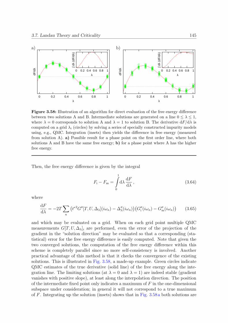
3.7. Landau Theory and Criticality 145
a) b)
0 0.2 0.4 0.6 0.8 1
dF/d
λ
λ
0 0.2 0.4 0.6 0.8 1∫ d
λ (d
F/d
λ)λ
0 0.2 0.4 0.6 0.8 1
dF/d
λ
λ
0 0.2 0.4 0.6 0.8 1
∫ dλ
(dF
/dλ)
λ
Figure 3.58: Illustration of an algorithm for direct evaluation of the free energy differencebetween two solutions A and B. Intermediate solutions are generated on a line 0 ≤ λ ≤ 1,where λ = 0 corresponds to solution A and λ = 1 to solution B. The derivative dF/dλ iscomputed on a grid λi (circles) by solving a series of specially constructed impurity modelsusing, e.g., QMC. Integration (insets) then yields the difference in free energy (measuredfrom solution A). a) Possible result for a phase point on the first order line, where bothsolutions A and B have the same free energy; b) for a phase point where A has the higherfree energy.
Then, the free energy difference is given by the integral
Fi − Fm =
1∫
0
dλdF
dλ, (3.64)
where
dF
dλ= −2T
∑
n
(t∗2G′′[T, U,∆λ](iωn)−∆′′
λ(iωn))(G′′
i (iωn)−G′′m(iωn)
)(3.65)
and which may be evaluated on a grid. When on each grid point multiple QMCmeasurements G[T, U,∆λ]i are performed, even the error of the projection of thegradient in the “solution direction” may be evaluated so that a corresponding (sta-tistical) error for the free energy difference is easily computed. Note that given thetwo converged solutions, the computation of the free energy difference within thisscheme is completely parallel since no more self-consistency is involved. Anotherpractical advantage of this method is that it checks the convergence of the existingsolutions. This is illustrated in Fig. 3.58, a made-up example. Green circles indicateQMC estimates of the true derivative (solid line) of the free energy along the inte-gration line. The limiting solutions (at λ = 0 and λ = 1) are indeed stable (gradientvanishes with positive slope), at least along the interpolation direction. The positionof the intermediate fixed point only indicates a maximum of F in the one-dimensionalsubspace under consideration; in general it will not correspond to a true maximumof F . Integrating up the solution (insets) shows that in Fig. 3.58a both solutions are

146 3. Mott Metal-Insulator Transition in the d→∞ Hubbard Model
stable, i.e., this phase point is on the first-order line while in Fig. 3.58b, the solutioncorresponding to λ = 1 is only metastable since the free energy is much higher (in-set). Even though the comparatively more conventional method of pinpointing thefirst-order transition line used in our numerical calculations also worked well, the newmethod suggested here seems significantly superior since it is fully local in U and Tand should be used in future work.48
Integrating the free energy in the solution space may also be useful for an absolutedetermination of F using some reference system. In particular, the impurity modelcorresponding to a Lorentzian DOS can be solved analytically and may serve asa reference point. Finally, the concept can obviously be generalized for arbitrarylattices. While for these cases, the lattice contribution to the free energy will haveto be computed numerically, the additional cost is still negligible in comparison withthe effort for solving the impurity model.
3.7.3 Critical Behavior Near the MIT
Two different aspects of criticality are potentially relevant in the context of studiesof the Mott metal-insulator transition: On the one hand, observables may showsingular behavior (i.e., have divergent slope as a function of T or U) near criticalpoints or critical lines. On the other hand, critical slowing down of the iterativeDMFT convergence process may arise within some regions of the parameter space.49
In principle, “raw” QMC results (i.e., results for fixed finite ∆τ) could be negativelyimpacted by critical slowing down while the accuracy of extrapolations and fits couldsuffer from our neglect to take singular behavior explicitly into account. We will inthis subsection discuss both effects and their relevance to the QMC studies presentedearlier in this chapter.
As pointed out by Kotliar et al. (2000), a second-order critical end point is sig-naled within the DMFT by the appearance of a single zero eigenvalue m0 of thefluctuation matrix (3.61) of the Ginzburg-Landau functional FGL.50 Under the as-sumption that this matrix smoothly depends on the hybridization function ∆n andon the parameters T and U , the associated eigenvector is well-defined also in thevicinity of the critical end point where it represents a soft mode. The associatedcoefficient η0 of an expansion of ∆n in terms of the eigen basis of the fluctuationmatrix then determines the critical behavior. In principle, critical exponents maybe calculated from Taylor expansions in η0. According to Kotliar et al. (2000), theparameter η0 may be replaced by another parameter η which fulfills a cubic equationwithout quadratic term, pη + cη3 = h, near the critical point. As a consequence,the double occupancy is predicted to show cubic-root behavior near the critical point
48As pointed out in more detail in Sec. 3.6, the transformation technique used by Tong et al. (2001)for determining the thermodynamic MIT line is directly related to the concepts of this subsection.In contrast to the method suggested here, however, the transformation technique incorporates anapproximation.
49Note that only the first consequence is strictly a property of the model; critical slowing downcould in principle be overcome by more advanced iteration techniques.
50All other eigenvalues are, then, negative since the minimum of FGL is unique for temperaturesat or above the critical point (cf. subsection 3.7.1).
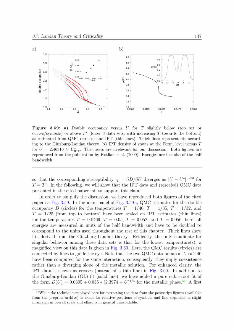
3.7. Landau Theory and Criticality 147
a) b)
2.1 2.2 2.3 2.4 2.5U
0.02
0.03
0.04
0.05
0.06
0.07
0.08
doub
le o
ccup
atio
n
−0.005 0.000 0.005 0.010[T−Tc]IPT
−0.005
0.000
0.005
0.010
[T−
Tc]
QM
C
0.0460 0.0465 0.0470 0.0475 0.0480T
0.0
0.2
0.4
0.6
0.8
1.0
1.2
1.4
1.6
1.8
ρ(0)
−3 −2 −1 0 1 2ω
0.0
0.2
0.4
0.6
0.8
ρ(ω)
Figure 3.59: a) Double occupancy versus U for T slightly below (top set orcurves/symbols) or above T ∗ (lower 3 data sets, with increasing T towards the bottom)as estimated from QMC (circles) and IPT (thin lines). Thick lines represent fits accord-ing to the Ginzburg-Landau theory. b) IPT density of states at the Fermi level versus Tfor U = 2.46316 ≈ U ∗
IPT. The insets are irrelevant for our discussion. Both figures arereproduced from the publication by Kotliar et al. (2000). Energies are in units of the halfbandwidth.
so that the corresponding susceptibility χ = ∂D/∂U diverges as |U − U ∗|−2/3 forT = T ∗. In the following, we will show that the IPT data and (rescaled) QMC datapresented in the cited paper fail to support this claim.
In order to simplify the discussion, we have reproduced both figures of the citedpaper as Fig. 3.59. In the main panel of Fig. 3.59a, QMC estimates for the doubleoccupancy D (circles) for the temperatures T = 1/40, T = 1/35, T = 1/32, andT = 1/25 (from top to bottom) have been scaled on IPT estimates (thin lines)for the temperatures T = 0.0469, T = 0.05, T = 0.052, and T = 0.056; here, allenergies are measured in units of the half bandwidth and have to be doubled tocorrespond to the units used throughout the rest of this chapter. Thick lines showfits derived from the Ginzburg-Landau theory. Evidently, the only candidate forsingular behavior among these data sets is that for the lowest temperature(s); amagnified view on this data is given in Fig. 3.60. Here, the QMC results (circles) areconnected by lines to guide the eye. Note that the two QMC data points at U ≈ 2.40have been computed for the same interaction; consequently, they imply coexistencerather than a diverging slope of the metallic solution. For enhanced clarity, theIPT data is shown as crosses (instead of a thin line) in Fig. 3.60. In addition tothe Ginzburg-Landau (GL) fit (solid line), we have added a pure cubic-root fit ofthe form D(U) = 0.0305 + 0.035 ∗ (2.3974 − U)1/3 for the metallic phase.51 A first
51While the technique employed here for extracting the data from the postscript figures (availablefrom the preprint archive) is exact for relative positions of symbols and line segments, a slightmismatch in overall scale and offset is in general unavoidable.
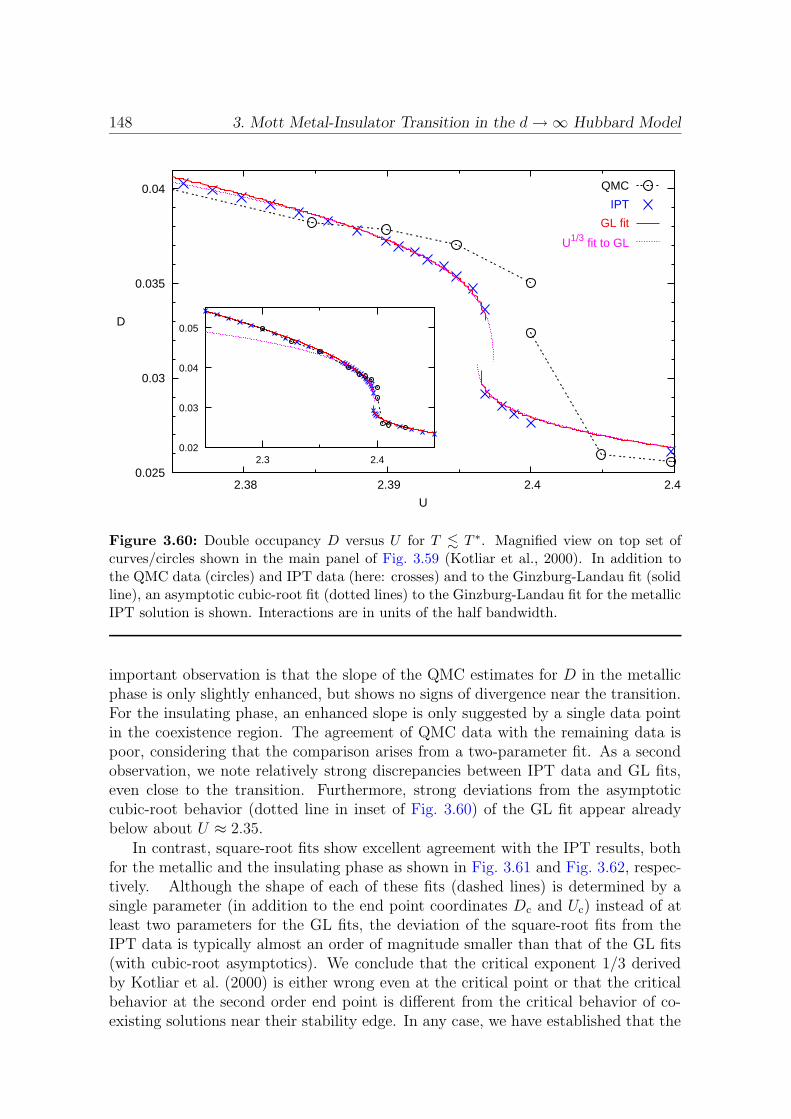
148 3. Mott Metal-Insulator Transition in the d→∞ Hubbard Model
0.025
0.03
0.035
0.04
2.38 2.39 2.4 2.41
D
U
QMC
IPT
GL fit
U1/3 fit to GL
0.02
0.03
0.04
0.05
2.3 2.4
Figure 3.60: Double occupancy D versus U for T . T ∗. Magnified view on top set ofcurves/circles shown in the main panel of Fig. 3.59 (Kotliar et al., 2000). In addition tothe QMC data (circles) and IPT data (here: crosses) and to the Ginzburg-Landau fit (solidline), an asymptotic cubic-root fit (dotted lines) to the Ginzburg-Landau fit for the metallicIPT solution is shown. Interactions are in units of the half bandwidth.
important observation is that the slope of the QMC estimates for D in the metallicphase is only slightly enhanced, but shows no signs of divergence near the transition.For the insulating phase, an enhanced slope is only suggested by a single data pointin the coexistence region. The agreement of QMC data with the remaining data ispoor, considering that the comparison arises from a two-parameter fit. As a secondobservation, we note relatively strong discrepancies between IPT data and GL fits,even close to the transition. Furthermore, strong deviations from the asymptoticcubic-root behavior (dotted line in inset of Fig. 3.60) of the GL fit appear alreadybelow about U ≈ 2.35.
In contrast, square-root fits show excellent agreement with the IPT results, bothfor the metallic and the insulating phase as shown in Fig. 3.61 and Fig. 3.62, respec-tively. Although the shape of each of these fits (dashed lines) is determined by asingle parameter (in addition to the end point coordinates Dc and Uc) instead of atleast two parameters for the GL fits, the deviation of the square-root fits from theIPT data is typically almost an order of magnitude smaller than that of the GL fits(with cubic-root asymptotics). We conclude that the critical exponent 1/3 derivedby Kotliar et al. (2000) is either wrong even at the critical point or that the criticalbehavior at the second order end point is different from the critical behavior of co-existing solutions near their stability edge. In any case, we have established that the

3.7. Landau Theory and Criticality 149
0.035
0.04
2.36 2.37 2.38 2.39 2.4
D
U
QMC
IPT
GL fit
U1/3 fit to GL
U1/2 fit to IPT
0.03
0.04
0.05
2.3 2.4
Figure 3.61: Double occupancy D versus U for T . T ∗. Magnified view on top set ofcurves/circles shown in the main panel of Fig. 3.59 (Kotliar et al., 2000) for the metal. Inaddition to the QMC and IPT data and to the Ginzburg-Landau fit, a cubic-root fit (dottedlines) and a square-root fit of the form D(U) = 0.0332 + 0.0488 (2.39695 − U)1/2 (dashedlines) to the asymptotic behavior of the metallic IPT solution is shown. Interactions are inunits of the half bandwidth.
latter is governed by an exponent of 1/2, at least within IPT.52
Given the fact that the misfit from the correct asymptotic behavior was hard tocatch even for IPT data which has no statistical error and even very close to thecritical end point, we may expect that critical behavior is practically undetectableusing QMC at temperatures that deviate by a few percent (or more) from the criticaltemperature T ∗ or when using a grid size of more than fractions of a percent inU . This is illustrated in Fig. 3.63 where the QMC data (symbols) presented byKotliar et al. (2000) is reanalyzed using regular fit functions (upper lines) similar tothose used in subsection 3.5.5. The bottom line shown for U ≥ 2.3 represents ourresult (3.19) for the insulator (rescaled to units of the half bandwidth). The slightsystematic deviation of the QMC data in the insulating phase (for U ≥ 2.4) from thiscurve probably reflects a finite ∆τ error. The overall agreement between QMC datafor the metallic phase and our fit functions is very good. For T = 1/40, below thecritical temperature, it is even much better than the agreement between QMC andeither the (rescaled) IPT result or the GL fit. Only the coexistence point belonging
52In contrast, the IPT result for the (interacting) density of states at the Fermi level shown inFig. 3.59b is well described by an exponent 1/3 when T is varied at constant U = U ∗
IPT, both onthe metallic and insulating side (with different prefactors).
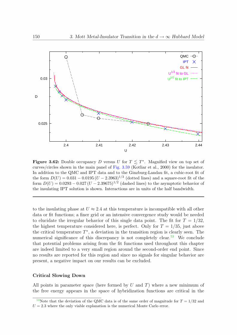
150 3. Mott Metal-Insulator Transition in the d→∞ Hubbard Model
0.025
0.03
2.4 2.41 2.42 2.43 2.44
D
U
QMC
IPT
GL fit
U1/3 fit to GL
U1/2 fit to IPT
Figure 3.62: Double occupancy D versus U for T . T ∗. Magnified view on top set ofcurves/circles shown in the main panel of Fig. 3.59 (Kotliar et al., 2000) for the insulator.In addition to the QMC and IPT data and to the Ginzburg-Landau fit, a cubic-root fit ofthe form D(U) = 0.031− 0.0195 (U − 2.3963)1/3 (dotted lines) and a square-root fit of theform D(U) = 0.0293− 0.027 (U − 2.39675)1/2 (dashed lines) to the asymptotic behavior ofthe insulating IPT solution is shown. Interactions are in units of the half bandwidth.
to the insulating phase at U ≈ 2.4 at this temperature is incompatible with all otherdata or fit functions; a finer grid or an intensive convergence study would be neededto elucidate the irregular behavior of this single data point. The fit for T = 1/32,the highest temperature considered here, is perfect. Only for T = 1/35, just abovethe critical temperature T ∗, a deviation in the transition region is clearly seen. Thenumerical significance of this discrepancy is not completely clear.53 We concludethat potential problems arising from the fit functions used throughout this chapterare indeed limited to a very small region around the second-order end point. Sinceno results are reported for this region and since no signals for singular behavior arepresent, a negative impact on our results can be excluded.
Critical Slowing Down
All points in parameter space (here formed by U and T ) where a new minimum ofthe free energy appears in the space of hybridization functions are critical in the
53Note that the deviation of the QMC data is of the same order of magnitude for T = 1/32 andU = 2.3 where the only viable explanation is the numerical Monte Carlo error.
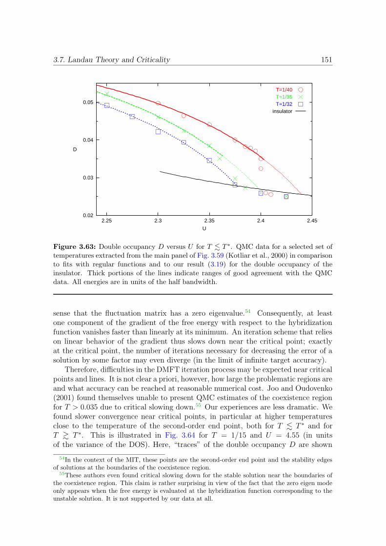
3.7. Landau Theory and Criticality 151
0.02
0.03
0.04
0.05
2.25 2.3 2.35 2.4 2.45
D
U
T=1/40T=1/35T=1/32
insulator
Figure 3.63: Double occupancy D versus U for T . T ∗. QMC data for a selected set oftemperatures extracted from the main panel of Fig. 3.59 (Kotliar et al., 2000) in comparisonto fits with regular functions and to our result (3.19) for the double occupancy of theinsulator. Thick portions of the lines indicate ranges of good agreement with the QMCdata. All energies are in units of the half bandwidth.
sense that the fluctuation matrix has a zero eigenvalue.54 Consequently, at leastone component of the gradient of the free energy with respect to the hybridizationfunction vanishes faster than linearly at its minimum. An iteration scheme that relieson linear behavior of the gradient thus slows down near the critical point; exactlyat the critical point, the number of iterations necessary for decreasing the error of asolution by some factor may even diverge (in the limit of infinite target accuracy).
Therefore, difficulties in the DMFT iteration process may be expected near criticalpoints and lines. It is not clear a priori, however, how large the problematic regions areand what accuracy can be reached at reasonable numerical cost. Joo and Oudovenko(2001) found themselves unable to present QMC estimates of the coexistence regionfor T > 0.035 due to critical slowing down.55 Our experiences are less dramatic. Wefound slower convergence near critical points, in particular at higher temperaturesclose to the temperature of the second-order end point, both for T . T ∗ and forT & T ∗. This is illustrated in Fig. 3.64 for T = 1/15 and U = 4.55 (in unitsof the variance of the DOS). Here, “traces” of the double occupancy D are shown
54In the context of the MIT, these points are the second-order end point and the stability edgesof solutions at the boundaries of the coexistence region.
55These authors even found critical slowing down for the stable solution near the boundaries ofthe coexistence region. This claim is rather surprising in view of the fact that the zero eigen modeonly appears when the free energy is evaluated at the hybridization function corresponding to theunstable solution. It is not supported by our data at all.

152 3. Mott Metal-Insulator Transition in the d→∞ Hubbard Model
0.038
0.039
0.04
0.041
0.042
0.043
0.044
0.045
0.046
0 10 20 30 40 50 60 70 80
D
iteration
∆τ=0.25
∆τ=0.20
∆τ=0.15
∆τ=0.10
Figure 3.64: Convergence of double occupancy D for T = 0.067 and U = 4.55. Thenumber of sweeps is about 105 for thin lines and about 106 for thick lines. Symbols at theleft axis indicate our best estimate of D for each value of ∆τ .
versus iteration number for several independent iteration runs. Line types (solid,long-dashed, short-dashed, and dotted) denote the time discretization ∆τ while thewidth of the lines give a rough indication of the numerical accuracy, i.e., the numberof sweeps used in each convergence run which is larger for thicker lines. Apparently,the overall convergence is not good since not all solutions for the same value of ∆τtend to a common fixed point. Instead, long-scale fluctuations appear, e.g., for therun with lower accuracy for ∆τ = 0.2 (thin long-dashed line). This is exactly what weexpect from Landau theory: as soon as the gradient of the free energy is smaller thanstatistical fluctuations, the iterated solutions follow an asymptotically free randomwalk (predominantly in the soft-mode direction). Two strategies for overcoming theassociated problems are also apparent from Fig. 3.64: On the one hand, it is importantto increase the numerical precision near critical regions in order to reduce fluctuations.On the other hand, trends can be much better recognized when comparing severalindependent self-consistency runs. By comparing the evolution (as a function ofiteration number) of different runs with more metallic or insulating initial conditions,one can establish boundaries for the fixed point or accelerate convergence by preparinginitial states near the assumed fixed point.56 We used such strategies extensivelythroughout the numerical parts of this thesis. For example, the upward trend ofinitial solutions for ∆τ = 0.15 (two lower short-dashed lines in Fig. 3.64) promptedus to initialize runs with D ≈ 0.042; those are seen to be stable.
In order to further illustrate these considerations and to demonstrate increasedfluctuations near the critical point, we perform sets of iteration runs for T = 0.055,
56The possibilities for initialization are obviously more limited very close to a stability edge.

3.7. Landau Theory and Criticality 153
0.038
0.039
0.04
0.041
0.042
0.043
0.044
0.045
0.046
0 5 10 15 20 25 30
D
iteration
∆τ=0.25∆τ=0.20∆τ=0.15
Figure 3.65: Convergence and fluctuations of double occupancy D for T = 0.055 andU = 4.65, very close to the critical end point (T ∗ = 0.055, U∗ = 4.665) for ∆τ = 0.0.Thin lines correspond to runs with 105 sweeps per iteration, thick lines to runs with 4 · 106
sweeps.
U = 4.65, i.e., very close to our estimate of the critical end point (for ∆τ = 0.0).Figure 3.65 shows results for the discretizations ∆τ = 0.25, ∆τ = 0.20, and ∆τ =0.15, with three statistically independent runs using 105 sweeps (“low” accuracy)and three runs using 4 · 106 sweeps per iteration (“high” accuracy) each. Evidently,the amplitude of fluctuations indeed increases for decreasing ∆τ at T = 0.055 andU = 4.65. The fluctuations are strongly reduced by a 40-fold increase in the numberof sweeps, i.e., by a reduction of the statistical error of the solution of each impuritymodel to about 1/6. Note that the long “time” scale (i.e., the large number ofiterations) associated with the fluctuations of the runs with low accuracy genericallyleads to an underestimation of error bars for averages obtained from a single run.One way of detecting such extremely long autocorrelation time is the comparison ofseveral independent runs as seen in Fig. 3.65 for ∆τ = 0.15. For a finite number ofruns, however, the deviations of all iteration runs may have the same sign as seen for∆τ = 0.20 in the same figure. Thus, accurate and controlled estimates can only beobtained from runs with high accuracy, i.e., a large number of sweeps.
Corresponding data for the slightly higher temperature T = 1/15 is shown inFig. 3.66. For each of the combinations of a representative sets of values of theinteraction (U = 4.4, U = 4.55, U = 4.65, and U = 4.8) and of the discretization (herelimited to ∆τ = 0.25, ∆τ = 0.2, and ∆τ = 0.15 by the computational resources), weused our best previous estimate of the converged solution for initializing 3 runs withhigh accuracy and 3 runs with low accuracy. While some initial trend is visible evenin some high accuracy runs, the rapid convergence of each run and the agreement

154 3. Mott Metal-Insulator Transition in the d→∞ Hubbard Model
a) b)
0.052
0.053
0.054
0.055
0 5 10 15 20
D
iteration
U=4.40.04
0.041
0.042
0.043
0.044
0.045
0.046
0.047
0 5 10 15 20
D
iteration
U=4.55
c) d)
0.03
0.031
0.032
0.033
0.034
0.035
0.036
0.037
0.038
0.039
0 5 10 15 20
D
iteration
U=4.650.0265
0.027
0.0275
0 5 10 15 20
D
iteration
U=4.8
Figure 3.66: Fluctuations in the double occupancy for T = 0.067 and a) U=4.4, b)U=4.55, c) U=4.65, and d) U=4.8 using a discretization of ∆τ = 0.25 (solid lines), ∆τ =0.2 (long-dashed lines), and ∆τ = 0.15 (short-dashed lines). Thin lines correspond to runswith 105 sweeps per iteration, thick lines to runs with 4 · 106 sweeps. Crosses at the leftaxis represent final estimates for D at finite ∆τ .
between the runs support the high accuracy of our final estimates.57 The goodconvergence of the final solutions (i.e., an average of the converged parts of the high-accuracy runs) is further supported independently by the regular dependence of Eon U (for each value of ∆τ) already seen in Fig. 3.23.
At lower temperatures, the fluctuations decay fast enough that runs with an orderof 105 sweeps suffice for reliable results. We conclude that critical slowing down posesa challenge which can be overcome by the techniques described here and by investing
57Note the vastly different scales for D in the different parts of Fig. 3.66.
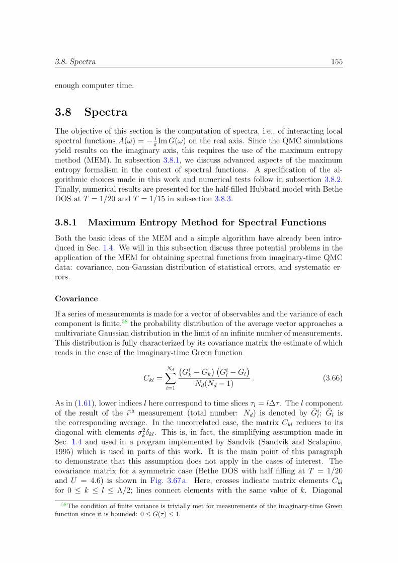
3.8. Spectra 155
enough computer time.
3.8 Spectra
The objective of this section is the computation of spectra, i.e., of interacting localspectral functions A(ω) = − 1
πImG(ω) on the real axis. Since the QMC simulations
yield results on the imaginary axis, this requires the use of the maximum entropymethod (MEM). In subsection 3.8.1, we discuss advanced aspects of the maximumentropy formalism in the context of spectral functions. A specification of the al-gorithmic choices made in this work and numerical tests follow in subsection 3.8.2.Finally, numerical results are presented for the half-filled Hubbard model with BetheDOS at T = 1/20 and T = 1/15 in subsection 3.8.3.
3.8.1 Maximum Entropy Method for Spectral Functions
Both the basic ideas of the MEM and a simple algorithm have already been intro-duced in Sec. 1.4. We will in this subsection discuss three potential problems in theapplication of the MEM for obtaining spectral functions from imaginary-time QMCdata: covariance, non-Gaussian distribution of statistical errors, and systematic er-rors.
Covariance
If a series of measurements is made for a vector of observables and the variance of eachcomponent is finite,58 the probability distribution of the average vector approaches amultivariate Gaussian distribution in the limit of an infinite number of measurements.This distribution is fully characterized by its covariance matrix the estimate of whichreads in the case of the imaginary-time Green function
Ckl =
Nd∑
i=1
(Gik − Gk
) (Gil − Gl
)
Nd(Nd − 1). (3.66)
As in (1.61), lower indices l here correspond to time slices τl = l∆τ . The l componentof the result of the ith measurement (total number: Nd) is denoted by Gi
l; Gl isthe corresponding average. In the uncorrelated case, the matrix Ckl reduces to itsdiagonal with elements σ2
kδkl. This is, in fact, the simplifying assumption made inSec. 1.4 and used in a program implemented by Sandvik (Sandvik and Scalapino,1995) which is used in parts of this work. It is the main point of this paragraphto demonstrate that this assumption does not apply in the cases of interest. Thecovariance matrix for a symmetric case (Bethe DOS with half filling at T = 1/20and U = 4.6) is shown in Fig. 3.67a. Here, crosses indicate matrix elements Cklfor 0 ≤ k ≤ l ≤ Λ/2; lines connect elements with the same value of k. Diagonal
58The condition of finite variance is trivially met for measurements of the imaginary-time Greenfunction since it is bounded: 0 ≤ G(τ) ≤ 1.

156 3. Mott Metal-Insulator Transition in the d→∞ Hubbard Model
a) b)
0
1
2
3
4
0 10 20 30 40 50 60 70 80 90 100
Ckl
/10-8
l
CklCll
0
0.1
0.2
0.3
0.4
0.5
0.6
0.7
0.8
0.9
1
0 10 20 30 40 50 60 70 80 90 100r k
l
l
rklrll
Figure 3.67: a) Covariance matrix Ckl of the QMC estimate of G(τ) for Bethe DOS,T = 1/20, U = 4.6, and ∆τ = 0.1 (i.e., Λ = 200) using 300 bins with 10000 sweeps each.Circles indicate diagonal elements Cll as a function of j; offdiagonal elements with the samevalue of k (crosses) are connected by a solid line. The indices extend over 0 ≤ k ≤ l ≤ Λ/2(and correspond to τk = k∆τ , τl = l∆τ); the missing elements follow from the symmetriesCkl = Clk and (here) G(τ) = G(β − τ). b) Corresponding Pearson’s coefficients rkl. Forenhanced clarity, only even indices are included in the plots.
elements are additionally denoted by circles. Evidently, the offdiagonal elements aregenerically of the same order of magnitude as the diagonal elements. This shows thatQMC measurements of the imaginary-time Green function G at different time slicesτl are not independent, but are instead highly correlated; in Bryan’s terminology thefull data set is oversampled. The same data is shown in a different representation inFig. 3.67b; here, each column and each row has been divided by the square root of thecorresponding diagonal element. The result is a matrix of Pearson’s coefficients rkl,a dimensionless measure of linear correlation between pairs of stochastic variables.
Corresponding plots of the covariance matrix for an asymmetric case (LDA DOSof La1-xSrxTiO3 , n = 0.94, T = 1/10, and U = 5.0) are shown in Fig. 3.68. Sinceall three bands are degenerate and since measurements of G for each band are highlycorrelated (e.g., the occupancy of individual bands fluctuates while the total occu-pancy is almost exactly constant), the most relevant covariance matrix for this caseis that shown in Fig. 3.68a for the band-averaged case; Fig. 3.68b which applies tomeasurements of G for one individual band (with much larger variances for τ → 0and τ → β) is included for comparison and for later discussion in chapter 5 (in sub-section 5.4.2). All results clearly demonstrate the large degree of covariance presentin QMC estimates of G(τ).
Thus, a more general formulation of the MEM should be used which takes intoaccount all elements of the covariance matrix. In principle, this is simple since theform (1.65) of the probability function still applies (in the limit of large bin size)
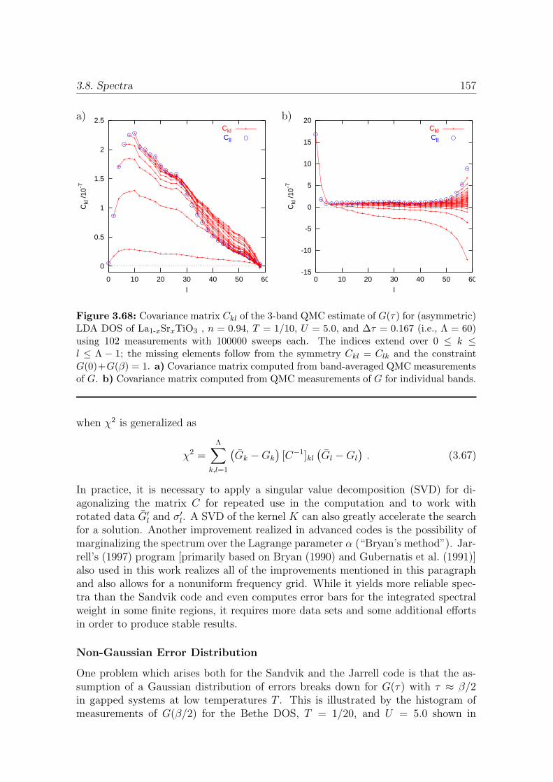
3.8. Spectra 157
a) b)
0
0.5
1
1.5
2
2.5
0 10 20 30 40 50 60
Ckl
/10-7
l
CklCll
-15
-10
-5
0
5
10
15
20
0 10 20 30 40 50 60
Ckl
/10-7
l
CklCll
Figure 3.68: Covariance matrix Ckl of the 3-band QMC estimate of G(τ) for (asymmetric)LDA DOS of La1-xSrxTiO3 , n = 0.94, T = 1/10, U = 5.0, and ∆τ = 0.167 (i.e., Λ = 60)using 102 measurements with 100000 sweeps each. The indices extend over 0 ≤ k ≤l ≤ Λ − 1; the missing elements follow from the symmetry Ckl = Clk and the constraintG(0)+G(β) = 1. a) Covariance matrix computed from band-averaged QMC measurementsof G. b) Covariance matrix computed from QMC measurements of G for individual bands.
when χ2 is generalized as
χ2 =Λ∑
k,l=1
(Gk −Gk
)[C−1]kl
(Gl −Gl
). (3.67)
In practice, it is necessary to apply a singular value decomposition (SVD) for di-agonalizing the matrix C for repeated use in the computation and to work withrotated data G′
l and σ′l. A SVD of the kernel K can also greatly accelerate the search
for a solution. Another improvement realized in advanced codes is the possibility ofmarginalizing the spectrum over the Lagrange parameter α (“Bryan’s method”). Jar-rell’s (1997) program [primarily based on Bryan (1990) and Gubernatis et al. (1991)]also used in this work realizes all of the improvements mentioned in this paragraphand also allows for a nonuniform frequency grid. While it yields more reliable spec-tra than the Sandvik code and even computes error bars for the integrated spectralweight in some finite regions, it requires more data sets and some additional effortsin order to produce stable results.
Non-Gaussian Error Distribution
One problem which arises both for the Sandvik and the Jarrell code is that the as-sumption of a Gaussian distribution of errors breaks down for G(τ) with τ ≈ β/2in gapped systems at low temperatures T . This is illustrated by the histogram ofmeasurements of G(β/2) for the Bethe DOS, T = 1/20, and U = 5.0 shown in

158 3. Mott Metal-Insulator Transition in the d→∞ Hubbard Model
0
100
200
300
400
500
600
700
800
900
0 0.01 0.02 0.03 0.04 0.05—G(β/2)
U=5.0U=4.7U=4.6
0
1000
2000
3000
4000
5000
0 0.001 0.002 0.003—G(β/2)
U=5.0, lower 97%
Figure 3.69: Histograms of G(β/2) for a Bethe DOS, T = 1/20, and ∆τ = 0.1 basedon 300 measurements for each value of U (boxes). Smooth lines indicate Gaussian fitsreproducing both the averages and the variances of each of the measured distributions.For U = 5.0, the variance is dominated by a small fraction of outliers; 97 percent of allmeasurements are below 0.003 (inset).
Fig. 3.69. Evidently, the distribution indicated by the histogram (boxes with solidlines) strongly differs from a Gaussian distribution corresponding to the same errorand variance. In particular, the true distribution is strongly asymmetric while theGaussian fit extends into the forbidden region G(β/2) < 0. In fact, the variance isprimarily associated with a small fraction of outliers [i.e., measurements correspond-ing to very large values of G(β/2)]; eliminating the top 3% of outliers results in amuch narrower (but still asymmetric) distribution as seen in the inset of Fig. 3.69.In comparison, the histograms for the insulating phase at U = 4.7 (dashed lines)and for the strongly correlated metallic phase at U = 4.6 (dotted lines) are muchbetter approximated by Gaussians. As a consequence, the application of the MEMformalism deep inside the insulating phase implies the use of an inappropriate like-lihood function59 unless the number and accuracy of measurements is increased (bysome orders of magnitude) so that Gaussian statistics is restored for the averages.60
MEM algorithms have been formulated, however, for non-Gaussian error statistics inother contexts (Bryan and Skilling, 1980); we are therefore confident that a practicalsolution could be found leading to even more reliable spectra for insulators.61
59Our attempt of solving this problem by transforming G (to a new unbounded variable) leadto severe numerical instabilities so that the corresponding method could not be used in practicalapplications.
60At this point, the statistical error may be lower than systematic errors so that potentially thefull error is never well approximated by a Gaussian distribution.
61Note that the presence of far outliers as seen for U = 5.0 in Fig. 3.69 poses an even moresevere problem than skew and kurtosis since the characterization of the corresponding probability

3.8. Spectra 159
Systematic Errors
It is important to realize that MEM can only yield reliable results when systematicerrors are much smaller than statistical errors. For DMFT calculations, systematicerrors can be caused by incomplete convergence of the self-consistency cycle andby a finite value of ∆τ . An accurate solution of the impurity problem and a largenumber of iterations (possibly using underrelaxation) can control the iteration error oreffectively convert it to a statistical error by using completely independent simulationruns. A similar effect is achieved at lesser cost by performing some additional DMFTiterations at very high precision after convergence; measurements of G(τ) for eachof the resulting impurity models can then be combined for analytic continuation.The spectra to be presented in this section will be based on 50 measurements for6 impurity models (i.e., a total of 300 bins) for each parameter set; this approachbrings the iteration error well under control.
In comparison, remaining ∆τ errors in Gl are potentially more severe. Sincethis problem cannot be overcome by extrapolation on the level of spectra, reliablespectra require good algorithms (i.e., programs with minimal ∆τ error) using smallenough values of ∆τ . This is more important in the context of DMFT calculationsthan for the solution of plain SIAMs since for the DMFT even the self-consistencycondition itself (which includes discretized Fourier transformations) introduces anerror at finite values of ∆τ (cf. subsection 3.4.1). For illustration of this point, acomparison of imaginary-time Green functions for the Bethe DOS in the insulatingphase (T = 1/20 and U = 5.0) is shown in Fig. 3.70. In order to resolve theimportant region of τ ≈ β/2, we here use a strongly magnified scale (for a morecomplete picture, see Fig. 3.75). The thick short-dashed line represents our bestestimate (for ∆τ = 0.1) of G(τ). The thinner dotted line is obtained by transformingback the MEM spectrum to be presented later in Fig. 3.80. The agreement betweenboth curves is excellent for τ . 6. Since the slight fluctuations visible in the QMCresults for 6 . τ ≤ 10 (with a local minimum for τ ≈ 7) violate analyticity,62 they arefiltered out by the MEM procedure which corresponds to a regularized form of G(τ)(dotted line). Both curves agree reasonably well with Jarrell’s result [for ∆τ = 0.167as used in Schlipf et al.’s (1999) paper: long-dashed line]. In contrast, Ulmke’soriginal smoothing trick discussed in subsection 3.4.1 leads to much larger G(τ) andfails to capture the insulating character of the solution: while the former results areroughly consistent with a gap of 0.5 (here modeled using rigid semi-elliptic Hubbardbands), the Ulmke-code solution implies quite significant spectral weight near ω = 0(which even exceeds that associated with touching rigid Hubbard bands).
We conclude that the most important prerequisite for computing reliable spectra
distribution is an ill-conditioned problem. We cannot exclude the possibility that the outliers areartifacts of the QMC method, i.e., arise from the finite number of warm-up sweeps used for eachmeasurement. Up to outliers, all data sets presented in Fig. 3.69 lead to nearly Gaussian histogramsof logG(β/2).
62The positivity of all even derivatives of G(τ) can be read off from (1.55); conversely, localextrema for 0 ≤ τ ≤ β/2 imply negative regions of the spectrum A(ω) which is clearly unphysical.A second, weaker form of the violation of analyticity may be detected when the computation of theself energy is attempted (see Sec. 4.6).
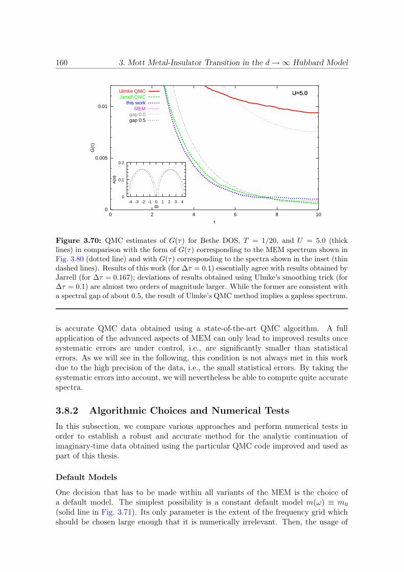
160 3. Mott Metal-Insulator Transition in the d→∞ Hubbard Model
0
0.005
0.01
0 2 4 6 8 10
G(τ
)
τ
U=5.0Ulmke QMCJarrell QMC
this workMEM
gap 0.0gap 0.5
0
0.1
0.2
-4 -3 -2 -1 0 1 2 3 4
A(ω
)
ω
U=5.0
Figure 3.70: QMC estimates of G(τ) for Bethe DOS, T = 1/20, and U = 5.0 (thicklines) in comparison with the form of G(τ) corresponding to the MEM spectrum shown inFig. 3.80 (dotted line) and with G(τ) corresponding to the spectra shown in the inset (thindashed lines). Results of this work (for ∆τ = 0.1) essentially agree with results obtained byJarrell (for ∆τ = 0.167); deviations of results obtained using Ulmke’s smoothing trick (for∆τ = 0.1) are almost two orders of magnitude larger. While the former are consistent witha spectral gap of about 0.5, the result of Ulmke’s QMC method implies a gapless spectrum.
is accurate QMC data obtained using a state-of-the-art QMC algorithm. A fullapplication of the advanced aspects of MEM can only lead to improved results oncesystematic errors are under control, i.e., are significantly smaller than statisticalerrors. As we will see in the following, this condition is not always met in this workdue to the high precision of the data, i.e., the small statistical errors. By taking thesystematic errors into account, we will nevertheless be able to compute quite accuratespectra.
3.8.2 Algorithmic Choices and Numerical Tests
In this subsection, we compare various approaches and perform numerical tests inorder to establish a robust and accurate method for the analytic continuation ofimaginary-time data obtained using the particular QMC code improved and used aspart of this thesis.
Default Models
One decision that has to be made within all variants of the MEM is the choice ofa default model. The simplest possibility is a constant default model m(ω) ≡ m0
(solid line in Fig. 3.71). Its only parameter is the extent of the frequency grid whichshould be chosen large enough that it is numerically irrelevant. Then, the usage of
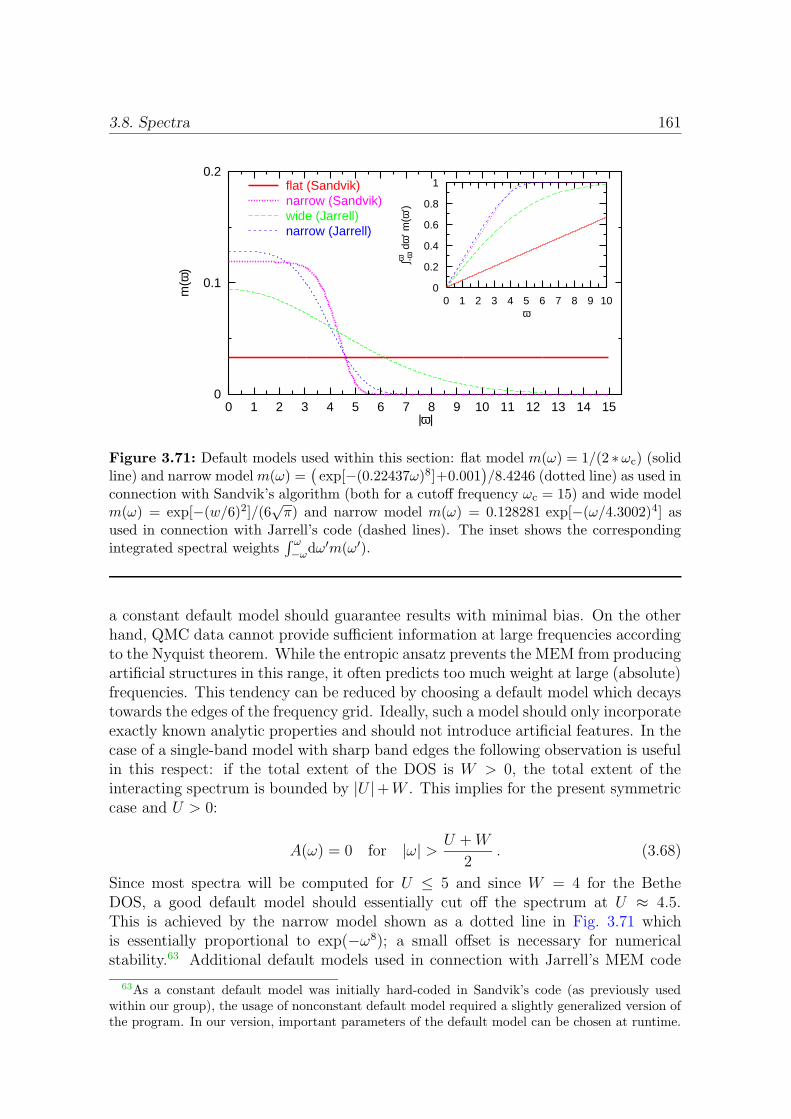
3.8. Spectra 161
0
0.1
0.2
0 1 2 3 4 5 6 7 8 9 10 11 12 13 14 15
m(ω
)
|ω|
flat (Sandvik)narrow (Sandvik)wide (Jarrell)narrow (Jarrell)
0
0.2
0.4
0.6
0.8
1
0 1 2 3 4 5 6 7 8 9 10
∫ω -ω d
ω’ m
(ω’)
ω
Figure 3.71: Default models used within this section: flat model m(ω) = 1/(2 ∗ωc) (solidline) and narrow modelm(ω) =
(exp[−(0.22437ω)8]+0.001
)/8.4246 (dotted line) as used in
connection with Sandvik’s algorithm (both for a cutoff frequency ωc = 15) and wide modelm(ω) = exp[−(w/6)2]/(6
√π) and narrow model m(ω) = 0.128281 exp[−(ω/4.3002)4] as
used in connection with Jarrell’s code (dashed lines). The inset shows the correspondingintegrated spectral weights
∫ ω−ωdω′m(ω′).
a constant default model should guarantee results with minimal bias. On the otherhand, QMC data cannot provide sufficient information at large frequencies accordingto the Nyquist theorem. While the entropic ansatz prevents the MEM from producingartificial structures in this range, it often predicts too much weight at large (absolute)frequencies. This tendency can be reduced by choosing a default model which decaystowards the edges of the frequency grid. Ideally, such a model should only incorporateexactly known analytic properties and should not introduce artificial features. In thecase of a single-band model with sharp band edges the following observation is usefulin this respect: if the total extent of the DOS is W > 0, the total extent of theinteracting spectrum is bounded by |U |+W . This implies for the present symmetriccase and U > 0:
A(ω) = 0 for |ω| > U +W
2. (3.68)
Since most spectra will be computed for U ≤ 5 and since W = 4 for the BetheDOS, a good default model should essentially cut off the spectrum at U ≈ 4.5.This is achieved by the narrow model shown as a dotted line in Fig. 3.71 whichis essentially proportional to exp(−ω8); a small offset is necessary for numericalstability.63 Additional default models used in connection with Jarrell’s MEM code
63As a constant default model was initially hard-coded in Sandvik’s code (as previously usedwithin our group), the usage of nonconstant default model required a slightly generalized version ofthe program. In our version, important parameters of the default model can be chosen at runtime.
162 3. Mott Metal-Insulator Transition in the d→∞ Hubbard Model
are shown as dashed lines in Fig. 3.71 and are specified in its caption.It is clearly possible to devise default models which represent more accurately
expectations about the true spectrum for the given parameter set, i.e., have featureslike upper and lower Hubbard bands, a quasiparticle peak or a gap at the Fermienergy etc. Such a default model can be obtained, e.g., as a result of approximatetheories, by fitting moments, or by using the MEM result of a related parameter set.In particular, Jarrell (1997) describes an annealing method which works at a hierarchyof temperatures: here, an analytic continuation of QMC data is first performed athigh temperatures where a default model obtained from perturbation theory is stillquite accurate. The MEM result obtained at each temperature step is then used as adefault model at the next lower temperature. While such a procedure can be justifiedfrom the observation that spectra usually depend smoothly on temperature and showmore structure at lower temperatures, it has no Bayesian foundation and may breakdown near phase transitions. In our view, the use of the annealing method shouldbe limited to cases where the MEM procedure cannot be stabilized by other means,possibly due to lack of sufficient computing resources. As we will see in the following,such a need does not arise within the context of this thesis.
We also will not need to apply generalizations of the MEM for enforcing analyticconstraints (i.e., for moments of the spectrum) by adding further terms to the loga-rithm of the prior probability defined in (1.63) (i.e., in connection with a Lagrangemultiplier). While such a procedure does not pose the danger of introducing artifacts,each enforced constraint removes one possible check of the accuracy of the result. Forthis reason and for the sake of simplicity, we prefer a plain implementation of theMEM (at least for comparison) in connection with sufficiently accurate data.64 Notethat the full band width can also be constrained by an appropriate choice of thedefault model.
Error Analysis
A first point that we would like to stress is the importance of performing the erroranalysis in the paramagnetic phase of interest for the spin-averaged data G(τ) =(G↑(τ) +G↓(τ))/2. By taking this average, the majority of statistical errors is elim-inated since in each QMC solution of the impurity problem the estimates of G↑(τ)and G↓(τ) are highly correlated. Due to the correlations, the alternative procedureof treating both estimates as independent measurements (as previously used in ourgroup) leads to incorrect error statistics; in fact, it grossly overestimates errors forsmall ∆τ (or small β−∆τ) which are here small due to the symmetry of the half-filledmodel. This is shown in the inset of Fig. 3.72 for T = 1/20 and U = 4.6. Here, thelower black solid line represents the true measured statistical error. Treating both
In Jarrell’s code, the default model (and even the grid) is completely arbitrary, since it is read froma specified file in tabulated form.
64In early stages of this work, we found violations of analytic behavior in MEM results whentrying to compute the real-frequency self-energy in antiferromagnetic phases. Here, the numericalMEM procedure can probably only be stabilized when some constraints are enforced. The followingnecessary conditions for analyticity valid for a Bethe lattice (W = 4) may be useful for future work:ImGα(ω) ImGα(ω) ≤ 1 and ImGα(ω)/ImGα(ω) ≥ ReG2
α(ω). Here, α denotes the sublattice index.

3.8. Spectra 163
0
0.1
0.2
0.3
0 1 2 3 4 5
A(ω
)
|ω|
T=1/20U=4.6
flatnarrownarrow, inc. errorflat, wrong errornarrow, wrong error
0
0.0002
0.0004
0.0006
0 1 2 3 4 5 6 7 8 9 10
∆— G(τ
)
τ
T=1/20U=4.6
Figure 3.72: Local spectral function A(ω) for T = 1/20 and U = 4.6: MEM resultsobtained using the Sandvik scheme based on statistical errors of spin-averaged QMC mea-surements (thick lines) or wrongly exaggerated errors (thin lines). Solid and dotted linescorrespond to a flat default model; dashed lines correspond to a narrow default model(cf. Fig. 3.71). Inset: errors estimated from spin-averaged measurements (lower lines) andexaggerated error (dotted line).
spin species as independent implies the error estimate shown as a dotted line whichincreases rapidly for τ → 0 (and extends to about 0.004 at τ = 0). The zig-zag curvealso shown in the inset of Fig. 3.72 takes additional systematic errors into accountas we will discuss below. The overestimation of errors at small τ implies that thisregion is essentially disregarded in the MEM continuation which suppresses the mostimportant information: on the one hand, higher-order moments of the spectrum aredirectly associated with derivatives G(n)(τ)|τ=0 via (1.59); on the other hand, theassumption of Gaussian error distribution is very accurate in this region.65 Theseconsiderations are clearly supported by the MEM results obtained using the Sandvikalgorithm shown in the main part of Fig. 3.72. Here, the solid and long-dashed linescorrespond to calculations based on the adjusted error (red solid line in the inset) forthe flat and the narrow default model detailed in Fig. 3.71, respectively. The excel-lent agreement between both results supports the good quality of the QMC data; the
65In fact, Jarrell recently suggested that QMC estimates of G(τ) should be disregarded in theproblematic region of τ ≈ β/2 in gapped phases in order to avoid negative impact of non-Gaussianerror statistics on the MEM results. In the symmetric case at hand, this suggestion would amountto using only QMC data at small τ (which is essentially disregarded in the scheme conventionallyemployed in our group).

164 3. Mott Metal-Insulator Transition in the d→∞ Hubbard Model
validity of both results is also supported by the fact that only little spectral weightis predicted in the region |ω| > 4.3 forbidden by (3.68). An additional result forthe narrow default model that takes into account the possibility of larger systematicerrors (short-dashed line) yields a somewhat more semi-elliptic shape of the Hubbardbands, but is overall consistent with the results discussed so far. In contrast, MEMresults based on the exaggerated error derived from unsymmetrized measurements(thinner curves) differ clearly: both the much stronger model dependence and thelarge weight at high frequencies indicate the poor quality of these results.
As we have pointed out in the beginning of this section, Jarrell’s program rep-resents a careful implementation of the Bayesian MEM approach and is in generalsuperior over simplified algorithms as implemented in the code originating from Sand-vik. Consequently, it would appear natural to only use the more advanced code forthis thesis. However, numerical instabilities were encountered in a direct applicationof this method to our best QMC data (for ∆τ = 0.1, i.e., Λ = 200 time slices), in par-ticular for very accurate data sets with small statistical errors. While some progresscould be made when the impact of the systematic iteration error was reduced by com-bining measurements performed for different impurity models (cf. subsection 3.8.1),consistent results could only be obtained by skipping time slices as illustrated inFig. 3.73. Here, best results (thick solid and dotted lines) were obtained by usingonly every 4th time slice (i.e., τ0 = 0, τ4 = 0.4 etc.) as can be seen from the rel-atively small dependence on the default model and from the comparison with the“Sandvik” result (double-dashed line) reproduced from Fig. 3.72. Skipping only ev-ery second time slice results in spectra (dashed lines) with additional features or toomuch weight at large frequencies; for a wide default model, even the analytic con-straint A(ω = 0) < 1/π is violated. When using the full QMC data as input, theMEM scheme did not even converge.66 A welcome side effect of skipping time slicesis that the overall impact of covariance is reduced which stabilizes the SVD.
The primary reason for these problems becomes apparent in the main panel ofFig. 3.74. Here, the imaginary-time Green function corresponding to the MEM spec-trum obtained from Sandvik’s method for a narrow default model (cf. Fig. 3.72) hasbeen subtracted from the measured QMC data. On the resulting magnified scale, anoscillatory behavior with deviations from a smooth curve which alternate on neigh-boring time slices becomes clearly visible. Since no such short-time oscillations appearin corresponding differences of Green functions associated [via (1.55)] with differentMEM spectra (not shown), the phenomenon is recognized as a systematic error ofthe QMC data. Most likely, this error is associated with remaining deficiencies ofthe Fourier transformation scheme employed in this work and could be removed byemploying a more sophisticated scheme as presented in App. C. While the individ-ual errors are roughly in line with estimated error bars (of about 10−4) for each timeslice, the pattern is so strong (in particular for small τ) that the associated unphysicaldegree of freedom can cause a failure of the full MEM procedure (in Jarrell’s code).On the other hand, the short-time oscillations are removed when only every secondor every fourth time slice is included in the analysis which explains why the stability
66In tests for other parameter sets where numerical convergence could be obtained, additionalseparated peaks and/or a central dip in the quasiparticle peak appeared in the spectra.
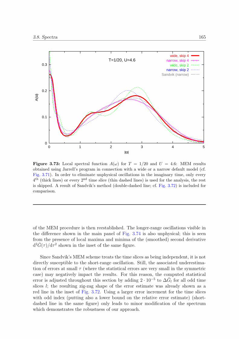
3.8. Spectra 165
0
0.1
0.2
0.3
0 1 2 3 4 5
A(ω
)
|ω|
T=1/20, U=4.6wide, skip 4
narrow, skip 4wide, skip 2
narrow, skip 2Sandvik (narrow)
Figure 3.73: Local spectral function A(ω) for T = 1/20 and U = 4.6: MEM resultsobtained using Jarrell’s program in connection with a wide or a narrow default model (cf.Fig. 3.71). In order to eliminate unphysical oscillations in the imaginary time, only every4th (thick lines) or every 2nd time slice (thin dashed lines) is used for the analysis, the restis skipped. A result of Sandvik’s method (double-dashed line; cf. Fig. 3.72) is included forcomparison.
of the MEM procedure is then reestablished. The longer-range oscillations visible inthe difference shown in the main panel of Fig. 3.74 is also unphysical; this is seenfrom the presence of local maxima and minima of the (smoothed) second derivatived2G(τ)/dτ 2 shown in the inset of the same figure.
Since Sandvik’s MEM scheme treats the time slices as being independent, it is notdirectly susceptible to the short-range oscillation. Still, the associated underestima-tion of errors at small τ (where the statistical errors are very small in the symmetriccase) may negatively impact the results. For this reason, the computed statisticalerror is adjusted throughout this section by adding 2 · 10−5 to ∆Gl for all odd timeslices l; the resulting zig-zag shape of the error estimate was already shown as ared line in the inset of Fig. 3.72. Using a larger error increment for the time sliceswith odd index (putting also a lower bound on the relative error estimate) (short-dashed line in the same figure) only leads to minor modification of the spectrumwhich demonstrates the robustness of our approach.

166 3. Mott Metal-Insulator Transition in the d→∞ Hubbard Model
-0.0001
0
0.0001
0.0002
0.0003
0.0004
0 1 2 3 4 5 6 7 8 9 10
— G(τ
) -
G(τ
) ME
M
τ
T=1/20, U=4.6
0
0.0002
0.0004
0.0006
0.0008
5 6 7 8 9
— G(2
) (τ)
τ
T=1/20, U=4.6
Figure 3.74: Difference between imaginary-time Green function G(τ) estimated by QMCand G(τ) corresponding to the MEM spectrum obtained using Sandvik’s scheme and a nar-row default model (solid line in Fig. 3.72). Inset: second derivative d2G(τ)/dτ2, smoothedwith Gaussian of width 0.3.
3.8.3 Numerical Results for the Bethe DOS
In this subsection, we present numerical results for the local spectral function of thehalf-filled Hubbard model with semi-elliptic DOS at moderately low temperatures(T = 0.05 and T = 0.067). These results are based on the MEM procedure discussedabove (using Sandvik’s scheme with properly adjusted errors) and on the QMC es-timates of the imaginary-time Green function shown in Fig. 3.75 for T = 0.05 andin Fig. 3.76 for T = 0.067. Using the symmetry G(β − τ) = G(τ), both figures aresplit for easier comparison of metallic solutions (left panel, only shown for τ ≤ β/2)and insulating solutions (right panel, only shown for τ ≥ β/2). Furthermore, thenoninteracting Green function (U = 0.0) is included for reference.
The spectra for the metallic phase at T = 0.05, i.e., slightly below the criticaltemperature T ∗ ≈ 0.055, are shown in Fig. 3.77 and Fig. 3.78 as obtained from MEMusing a flat and a narrow default model, respectively. The corresponding results forthe insulating phase are depicted in Fig. 3.79 and Fig. 3.80. Evidently, the dependenceof the spectra on the default model is negligible for all interactions U presented inthe graphs. In the metallic phase, the spectral density at the Fermi level (ω = 0)is approximately pinned at the noninteracting value ρ(0) = 1/π ≈ 0.32 for U . 4.4.Since Luttinger’s theorem is exact only at T = 0, the slight deviation in this Fermiliquid regime can be attributed to the finite temperature. The larger deviation for
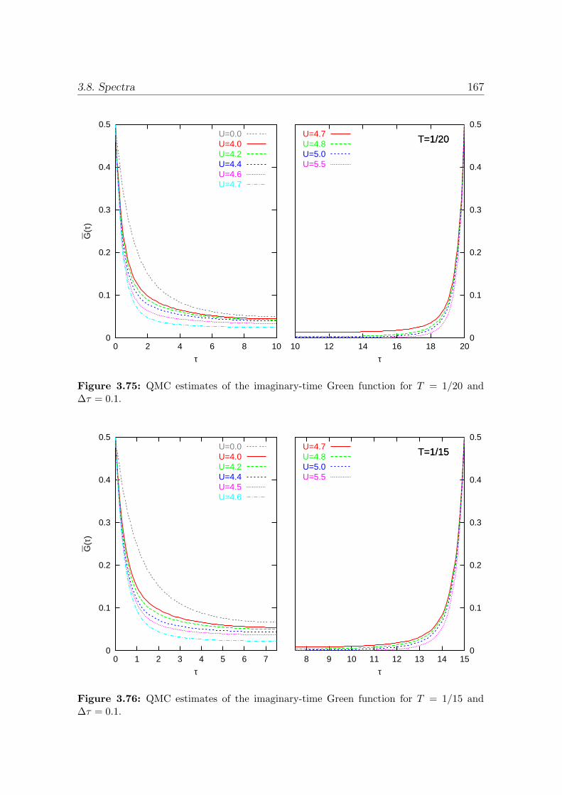
3.8. Spectra 167
0
0.1
0.2
0.3
0.4
0.5
0 2 4 6 8 10
— G(τ
)
τ
T=1/20U=0.0U=4.0U=4.2U=4.4U=4.6U=4.7
10 12 14 16 18 200
0.1
0.2
0.3
0.4
0.5
τ
T=1/20U=4.7U=4.8U=5.0U=5.5
Figure 3.75: QMC estimates of the imaginary-time Green function for T = 1/20 and∆τ = 0.1.
0
0.1
0.2
0.3
0.4
0.5
0 1 2 3 4 5 6 7
— G(τ
)
τ
T=1/15U=0.0U=4.0U=4.2U=4.4U=4.5U=4.6
8 9 10 11 12 13 14 150
0.1
0.2
0.3
0.4
0.5
τ
T=1/15U=4.7U=4.8U=5.0U=5.5
Figure 3.76: QMC estimates of the imaginary-time Green function for T = 1/15 and∆τ = 0.1.
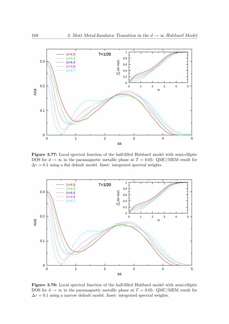
168 3. Mott Metal-Insulator Transition in the d→∞ Hubbard Model
0
0.1
0.2
0.3
0 1 2 3 4 5
A(ω
)
|ω|
T=1/20U=4.0U=4.2U=4.4U=4.6U=4.7
0
0.2
0.4
0.6
0.8
1
0 1 2 3 4 5
∫ω -ω d
ω’ A
(ω’)
ω
T=1/20
Figure 3.77: Local spectral function of the half-filled Hubbard model with semi-ellipticDOS for d → ∞ in the paramagnetic metallic phase at T = 0.05: QMC/MEM result for∆τ = 0.1 using a flat default model. Inset: integrated spectral weights.
0
0.1
0.2
0.3
0 1 2 3 4 5
A(ω
)
|ω|
T=1/20U=4.0U=4.2U=4.4U=4.6U=4.7
0
0.2
0.4
0.6
0.8
1
0 1 2 3 4 5
∫ω -ω d
ω’ A
(ω’)
ω
T=1/20
Figure 3.78: Local spectral function of the half-filled Hubbard model with semi-ellipticDOS for d → ∞ in the paramagnetic metallic phase at T = 0.05: QMC/MEM result for∆τ = 0.1 using a narrow default model. Inset: integrated spectral weights.
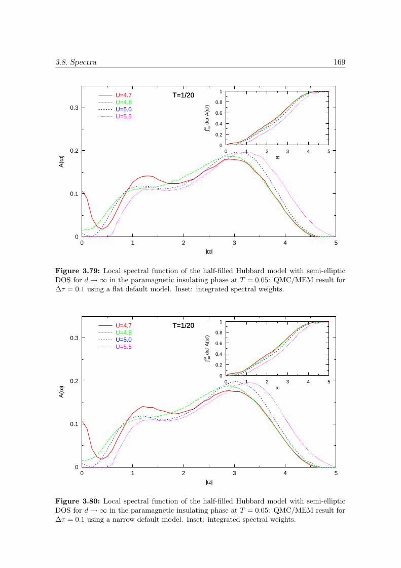
3.8. Spectra 169
0
0.1
0.2
0.3
0 1 2 3 4 5
A(ω
)
|ω|
T=1/20U=4.7U=4.8U=5.0U=5.5
0
0.2
0.4
0.6
0.8
1
0 1 2 3 4 5
∫ω -ω d
ω’ A
(ω’)
ω
T=1/20
Figure 3.79: Local spectral function of the half-filled Hubbard model with semi-ellipticDOS for d→∞ in the paramagnetic insulating phase at T = 0.05: QMC/MEM result for∆τ = 0.1 using a flat default model. Inset: integrated spectral weights.
0
0.1
0.2
0.3
0 1 2 3 4 5
A(ω
)
|ω|
T=1/20U=4.7U=4.8U=5.0U=5.5
0
0.2
0.4
0.6
0.8
1
0 1 2 3 4 5
∫ω -ω d
ω’ A
(ω’)
ω
T=1/20
Figure 3.80: Local spectral function of the half-filled Hubbard model with semi-ellipticDOS for d→∞ in the paramagnetic insulating phase at T = 0.05: QMC/MEM result for∆τ = 0.1 using a narrow default model. Inset: integrated spectral weights.
170 3. Mott Metal-Insulator Transition in the d→∞ Hubbard Model
U = 4.6 may be exaggerated due to the finite frequency grid ∆ω = 0.1 (which is herealready of the same order of magnitude as the width of the quasiparticle peak). Theclearly reduced peak hight at U = 4.7, however, marks the destruction of the Fermiliquid. For this value of the interaction, an additional shoulder or peak appears ineach Hubbard band. As seen from the integrated spectral weights shown in the insetsof Fig. 3.77 and Fig. 3.78, the main difference between the spectra for U = 4.6 andU = 4.7 is a shift of spectral weight of about 0.05 from |ω| . 0.5 to |ω| & 0.5.
The spectra corresponding to the insulating phase at U = 4.7 shown in Fig. 3.79and Fig. 3.80 do not follow the expected form. In fact, the remnant of a quasiparticlepeak points to a more metallic character. Since U = 4.7 is right at the edge ofthe stability region for T = 0.05 and ∆τ = 0.1 as previously seen in Fig. 3.24, thisfact may be due to numerical errors (although the corresponding QMC solution hasbeen found to be stable for some 20 iterations). Such ambiguities are absent forU ≥ 4.8: a pseudogap with very low residual spectral weight appears for U = 4.8.Within the numerical accuracy, the spectrum for U = 5.0 is already gapped with agap size of about 0.5 which is in line with the estimate obtained in Fig. 3.70. Thegap size increases to about 1.2 for U = 5.5. A shoulder or two-peak structure ofthe Hubbard band is seen in all results for the highly correlated metallic phase andfor the insulating phase which supports the genuineness of this feature. It does notbecome more pronounced with increasing interaction (in the insulating phase), butis slightly reduced from U = 5.0 to U = 5.5. Such a behavior is expected since rigidsemi-elliptic Hubbard bands (of widths W and centered around ω = ±U/2) have tobe recovered for U →∞ (Gebhard, 1997).
Results for T = 0.067, i.e., above the critical temperature, are shown in Fig. 3.81for the more metallic phase and in Fig. 3.82 for the more insulating phase. We cau-tion the reader that these results have not been checked as carefully as the precedingresults (for T = 0.05). We still expect the following observations to be genuine. Itis seen in Fig. 3.81 that the height of the quasiparticle peak decreases significantlywith increasing U already for 4.0 . U . 4.5. Thus, the Fermi liquid phase breaksdown before the crossover towards the insulator (defined in terms of the energy de-pendence; cf. Fig. 3.23) takes place at U ≈ 4.62. Again, the appearance of a secondpeak in the Hubbard band is associated with the disappearance of the quasiparticlepeak, here for U = 4.6. On the insulating side, the gap opens very slowly; significantspectral weight is still present at |ω| ≈ 0 for U = 4.7 and U = 4.8. Deep inside theinsulating phase at U = 5.0 and U = 5.5, however, the spectra are quite similar tothe spectra computed for T = 0.05 with gap sizes of about 0.5 and 1.2, respectively.The temperature independence of the spectra in the insulating phase is in line withthe corresponding observation of such independence made for the energy and thedouble occupancy in subsection 3.5.2.
Finally, let us compare the spectra computed within this thesis with previouslypublished work. Fig. 3.83a reproduces spectra for T = 0.05 computed by Jarrelland included in our joint publication (Schlipf et al., 1999). Considering the slightdifference in the imaginary-time discretization used by Jarrell (∆τ = 0.167 versus∆τ = 0.1 for our results), the overall agreement is reasonable. The better agreementwith Luttinger’s theorem for U = 4.0 may be due to the finer frequency grid used by
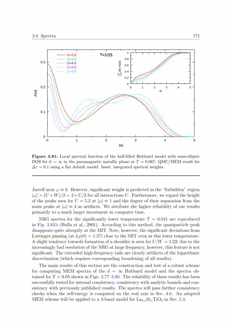
3.8. Spectra 171
0
0.1
0.2
0.3
0 1 2 3 4 5
A(ω
)
|ω|
T=1/15U=4.0U=4.2U=4.4U=4.5U=4.6
0
0.2
0.4
0.6
0.8
1
0 1 2 3 4 5
∫ω -ω d
ω’ A
(ω’)
ω
T=1/15
Figure 3.81: Local spectral function of the half-filled Hubbard model with semi-ellipticDOS for d → ∞ in the paramagnetic metallic phase at T = 0.067: QMC/MEM result for∆τ = 0.1 using a flat default model. Inset: integrated spectral weights.
Jarrell near ω ≈ 0. However, significant weight is predicted in the “forbidden” region|ω| > (U +W )/2 = 2+U/2 for all interactions U . Furthermore, we regard the heightof the peaks seen for U = 5.2 at |ω| ≈ 1 and the degree of their separation from themain peaks at |ω| ≈ 3 as artifacts. We attribute the higher reliability of our resultsprimarily to a much larger investment in computer time.
NRG spectra for the significantly lower temperature T = 0.041 are reproducedin Fig. 3.83b (Bulla et al., 2001). According to this method, the quasiparticle peakdisappears quite abruptly at the MIT. Note, however, the significant deviations fromLuttinger pinning (at 4 ρ(0) = 1.27) close to the MIT even at this lower temperature.A slight tendency towards formation of a shoulder is seen for U/W = 1.22; due to theincreasingly bad resolution of the NRG at large frequency, however, this feature is notsignificant. The extended high-frequency tails are clearly artifacts of the logarithmicdiscretization (which requires corresponding broadening of all results).
The main results of this section are the construction and test of a robust schemefor computing MEM spectra of the d = ∞ Hubbard model and the spectra ob-tained for T = 0.05 shown in Figs. 3.77–3.80. The reliability of these results has beensuccessfully tested for internal consistency, consistency with analytic bounds and con-sistency with previously published results. The spectra will pass further consistencychecks when the self-energy is computed on the real axis in Sec. 4.6. An adaptedMEM scheme will be applied to a 3-band model for La1-xSrxTiO3 in Sec. 5.4.

172 3. Mott Metal-Insulator Transition in the d→∞ Hubbard Model
0
0.1
0.2
0.3
0 1 2 3 4 5
A(ω
)
|ω|
T=1/15U=4.7U=4.8U=5.0U=5.5
0
0.2
0.4
0.6
0.8
1
0 1 2 3 4 5
∫ω -ω d
ω’ A
(ω’)
ω
T=1/15
Figure 3.82: Local spectral function of the half-filled Hubbard model with semi-ellipticDOS for d → ∞ in the paramagnetic insulating phase at T = 0.067: QMC/MEM resultfor ∆τ = 0.1 using a flat default model. Inset: integrated spectral weights.
a) b)
−6 −4 −2 0 2 4 6ω
0
0.1
0.2
0.3
0.4
A(ω
)
U=4.0U=4.6U=4.8U=5.0U=5.2
−1.5 −1.0 −0.5 0.0 0.5 1.0 1.5ω/W
0.0
0.5
1.0
A(ω
)∗W
U/W=1.17U/W=1.15U/W=1.13
0.0
0.5
1.0
A(ω
)∗W
U/W=1.18U/W=1.20U/W=1.22
a: increasing U
b: decreasing U
Figure 3.83: Local spectral function of the half-filled Hubbard model with semi-ellipticDOS for d → ∞ in the paramagnetic phase: a) QMC/MEM results for T = 0.05 (and∆τ = 0.167) obtained by Jarrell [figure adapted from Schlipf et al. (1999)]. b) NRG resultsfor T = 0.041 (using the scale W = 4 of this work) published by Bulla et al. (2001).
3.9. Conclusion 173
3.9 Conclusion
In this chapter, we have studied the fully frustrated half-filled Hubbard model witha semi-elliptic noninteracting density of states in the limit of infinite dimensionalitynear the Mott metal-insulator transition (MIT).
We have computed the coexistence region of metallic and insulating phases withsignificantly higher accuracy than achieved previously in the literature. In the courseof this study, we have discussed the signatures of a first-order transition within theDMFT and for the first time established a rigorous relation between the stability offixed points in a DMFT iteration scheme and the thermodynamic (meta-) stability ofphases. Using an improved method for the quantum Monte Carlo (QMC) calculationof the kinetic energy, we have presented the first accurate estimates of the full energy(per electron) and have shown that this observable is far better suited for the QMCdetermination of phase boundaries than other observables considered so far. We haveexplained the initial contradiction between QMC results regarding the possible extentof the coexistence region by identifying strengths and weaknesses of the QMC codesand strategies used by the major groups in the field. In particular, we have foundand corrected a major flaw in the QMC code used previously by our group; whilethe original code was already correct in the limit of vanishing discretization ∆τ → 0,it had introduced an unnecessary error at small frequencies which suppressed thecoexisting insulating phase at attainable values of ∆τ . We have also parallelized theQMC code in order to efficiently use all available computing resources.
While the coexistence of metallic and insulating solutions indicates the presenceof a first-order transition, the phase diagram is only complete with the determina-tion of the thermodynamic first-order transition line Uc(T ). This task was previouslyregarded as too difficult for numerically exact methods that cannot directly computethe free energy of the impurity model (such as QMC and NRG); even the predic-tion of the iterative perturbation theory was initially unclear. We have derived afirst-order differential equation for the phase boundary; its solution is more stablethan a more direct comparison of free energies due to the cancellation of errors. Onthe basis of highly accurate measurements for the energy and the double occupancy,we have established that the differential equation may be linearized without loss ofaccuracy. We have derived the leading low-temperature asymptotics of Uc(T ) fromFermi liquid theory and have fixed a numerical coefficient by calculating the groundstate properties of the metallic phase. This was possible by performing an interpo-lating fit of new (zero-temperature) second-order perturbation theory estimates withresults for Uc(T = 0) previously obtained by ground state methods. The quality ofthis fit has been stabilized by demanding thermodynamic consistency and has beensuccessfully tested by comparison with extrapolated QMC data. As a byproduct, wehave calculated the coefficient γ(U) of the low-temperature specific heat and checkedthe consistency with extrapolated estimates for the quasiparticle weight Z. Due tothe high precision of the QMC data and the numerous independent checks, the accu-racy of the resulting first controlled estimate of the thermodynamic first-order phasetransition line is well established.
We have analyzed Tong et al.’s (2001) recently published independent estimates
174 3. Mott Metal-Insulator Transition in the d→∞ Hubbard Model
for the first-order phase transition line based on a scheme using a modified set of self-consistency equations. While the agreement on the level of Uc(T ) is impressive, wehave found significant discrepancies with respect to the measured double occupancieswhich this group had used in a Maxwell construction for Uc(T ). In addition, wehave demonstrated the approximate character of this scheme. We have also studiedsignatures of critical behavior and have found that its impact on QMC studies islimited to the close surroundings of the (finite-temperature) critical end point of thefirst-order line. In addition, we have reanalyzed IPT data for the double occupancyin the critical region and have demonstrated that it is governed by a critical exponentof 1/2 rather than the value of 1/3 obtained by Kotliar et al. (2000).
Finally, we have discussed the maximum entropy method (MEM) and its applica-tion to the analytic continuation of imaginary-time Green functions computed withinQMC. We have demonstrated the strong improvement resulting from our correctionof the QMC code and devised a robust MEM scheme that takes the remaining sys-tematic errors into account. By applying this method to large sets of precise QMCmeasurements, we have calculated the first low-temperature MEM spectra in theMIT region which do not depend on specially chosen (“annealed”) default models.The overall high precision of the results is indicated by the good agreement with an-alytical bounds for the total bandwidth and by the excellent agreement with a sumrule for the derived real-frequency self-energy (to be discussed in Sec. 4.6).
In view of the excellent internal consistency of our results and the good agreementwith data obtained using other methods (within their respective error bars), our finalphase diagram Fig. 3.50 and other results presented in this chapter should representa fairly precise and complete picture of the local properties of the fully frustratedmodel. However, they clearly do not represent a complete scenario for any materialfeaturing a MIT. This follows already from the finite ground-state entropy predictedin the insulating phase which violates Nernst’s law. A more realistic and consistentdescription is possible when the low-temperature phase is ordered already in d =∞,i.e., for partial frustration. Analytical considerations for the consequences in the caseof varying partial frustration at constant semi-elliptic DOS have been presented inthis chapter. Investigations whether a phase diagram with a topology analogous tothat seen in V2O3 can also be observed in the generic case that frustration induces anasymmetry of the DOS have recently been initiated under our supervision (Knecht,2002); at present, this question is still open.
A further significant improvement of the QMC code based on ideas developedin this thesis and implemented by Knecht (2002) is briefly discussed in App. C;numerical comparisons shown in this appendix also demonstrate the high accuracy ofthe (less general) approach employed within this work. Future DMFT studies couldalso greatly profit from a scheme for the direct evaluation of differences in the freeenergy of coexisting solutions developed in this chapter.
175
Chapter 4
Optical Conductivity
In this chapter, we will discuss electronic transport, in particular the (q = 0) opticalconductivity σ(ω). Transport properties are not only very important technologically,but can also be probed accurately by a variety of techniques. As we will see below,measurements, e.g., of reflectivity, electronic energy loss, and of the direct-current(dc) conductivity are, thus, valuable tools for determining the electronic structureof materials. Specifically, a metal-insulator transition as discussed in chapter 3 issignaled by a vanishing Drude weight, i.e., a suppression of σ(ω) at low frequencies(and specifically for ω = 0).1
We will here focus on the exact theory of transport strictly in the limit of infinitedimensionality (d → ∞) or, more generally, infinite lattice coordination number(Z →∞), but also mention implications for an approximate treatment of the finite-dimensional case. Since all directional transport vanishes in infinite dimensions,2 e.g.,
σxx(ω)d→∞−→ 0 +O(1/d) (4.1)
for the optical conductivity in x direction, we will consider leading corrections, e.g.,dσxx(ω) or
∑
α σαα(ω). While the fact that most unscaled transport properties vanishin high dimensions might be viewed as a conceptual complication, their computationis much simplified in this limit: due to the effective locality of the vertex function (forq = 0), their diagrammatic expressions reduce to the bubble diagram. Consequently,σ(ω) can be evaluated from the full interacting Green function and the unrenor-malized current vertex. It is important to note that the current vertex introducesa dependence on lattice structure and hopping parameters beyond the noninteract-ing DOS so that models which are equivalent in the DMFT with respect to localproperties may differ significantly in terms of transport properties. In fact, we willshow in this chapter that σ(ω) is not uniquely defined on “the Bethe lattice”, i.e., on
1In principle, we could have used results for σ(ω) in order to determine the MIT transition linesUc1 and Uc2 in chapter 3. The attainable accuracy is, however, much better for the energy E and forthe double occupancy D since these observables do not require an analytic continuation via MEM.
2Strictly speaking, this statement only applies to total or partial weights, i.e., integrals over finitefrequency ranges and only when the lattice is essentially isotropic, i.e., when the kinetic energy is notdominated by a subset of directions. In particular, the limits ω → 0 and d→∞ do not necessarilycommute.

176 4. Optical Conductivity
lattices having a semi-elliptic DOS for Z → ∞ (cf. Sec. 2.2) and present formalismand results for several possible choices. We will demonstrate why some approachesfail to describe coherent transport and that the extended-hopping general-dispersionapproach proposed in Sec. 2.3 produces the physically most desirable results.
As indicated above, the numerical results of this chapter correspond to a consis-tent theory which is exact in d =∞. We will also point out how one may alternativelyuse the formalism as a local approximation in finite dimensions, e.g., in connectionwith LDA calculations (cf. subsection 5.4.3). We will not, however, discuss vertexcorrections which may change the picture completely in d = 3 or even lower dimen-sions.
The remainder of this chapter is structured as follows: In Sec. 4.1, we introduceσ(ω) and other dielectric quantities on a phenomenological level, collect relevant sumrules, point out the relation to experimental results, and discuss the impact of modelabstractions. The Kubo formalism is reviewed in Sec. 4.2 both for continuum andlattice models. The simplifications arising in d→∞ are discussed in Sec. 4.3 wherewe will also point out that the formalism widely used in the literature so far is veryspecific to the hypercubic lattice and must be modified in the general case. Variants ofthe general formalism applicable to tight-binding models with a semi-elliptic densityof states are studied in Sec. 4.4. Generalizations to models with varying degree ofcoherence and to finite dimensions as well as the theory of transport properties forfrustrated lattices with t − t′ hopping are discussed in Sec. 4.5. Finally, we presentnumerical results for the Hubbard model with semi-elliptic DOS in Sec. 4.6.
4.1 Definition and General Properties of the
Optical Conductivity
If a system is subjected to an external electric field then, in general, a redistributionof charges occurs and currents are induced. For small enough fields, the inducedpolarization and the induced currents are proportional to the inducing field. If theHamiltonian of the unperturbed system is not explicitly time-dependent, we havespecifically for the total current density in linear response,
Jα(r, t) =∑
β
∫
dr′t∫
−∞
dt′ σαβ(r, r′, t− t′)Eβ(r′, t′), (4.2)
where α, β label space directions and E is the (total) electric field. If the system is ho-mogeneous above some length scale a (e.g., for a lattice spacing a), then the responseto perturbations which are slowly varying on this length scale is also homogeneous,
Jα(r, t) =∑
β
∫
dr′t∫
−∞
dt′ σαβ(r − r′, t− t′)Eβ(r′, t′), (4.3)
4.1. Definition and General Properties of the Optical Conductivity 177
which can be Fourier-transformed to yield
Jα(q, ω) =∑
β
σαβ(q, ω)Eβ(q, ω). (4.4)
Since photons have a much steeper (linear) energy dispersion than electrons withinthe Brillouin zone, the transmitted momentum is essentially zero for not too highenergies. Thus, in the optical frequency regime and below we can take the long-wavelength limit q → 0. For cubic symmetry, the response is then isotropic, i.e., theconductivity tensor becomes diagonal:3
J(ω) = σ(ω)E(ω). (4.5)
Note that causality, i.e., the restriction to t′ < t in (4.2) and (4.3), implies a retardedconductivity σ(ω) which is analytic in the upper half plane.
4.1.1 Connection between Conductivity and Reflectivity
Under the conditions used in the derivation of (4.4), the dielectric function ε(ω)is defined as relating the (coarse-grained) electrical displacement D to the (coarse-grained) electric field E,4
D(ω) = ε(ω)E(ω). (4.6)
The dielectric function can be directly expressed in terms of the optical conductivity,
ε(ω) = 1 +4πiσ(ω)
ω. (4.7)
Note that here σ(ω) here has the dimension of a frequency (or energy) which is onlyvalid in the Gaussian system of units. Also note the importance of the absolute scaleof σ(ω) which determines qualitative features of ε(ω) as, e.g., the zeros of ε1(ω). Forlater use, we also state the equivalent equation valid in the SI system [ε → ε/ε0,σ → σ/(4πε0)]
εSI(ω) = ε0 +iσ(ω)
ω; ε0 = 8.85× 10⁻¹² Fm−1 = 8.85× 10⁻¹² s
Ωm. (4.8)
In some cases, solids can be prepared in thin enough slices that absorption andphase shift can be directly measured in transmission experiments in the energyranges of interest. Then, the index of diffraction n(ω) determines the phase ve-locity cmedium(ω) = c/n(ω), i.e., the phase shift in a sample of finite thickness, whilek(ω) quantifies the absorption per wavelength [see, e.g., Hecht (1997) or Landau andLifschitz (1990)]. The functions ε(ω) and σ(ω) are obtained from such measurementsvia
κ(ω) ≡√
ε(ω) = n(ω) + ik(ω) , (4.9)
3This is not true at finite q, even in an homogeneous system. Later, in Sec. 4.4, we will also needto consider the more general case where σ(ω) is still diagonal, but not isotropic.
4Unless stated otherwise, we will here and in the following use the Gaussian system of units(cgs).

178 4. Optical Conductivity
where the square root is taken such that n is positive, and via (4.7).If transmission experiments are not possible, but at least good (i.e., smooth and
clean) surfaces can be prepared, then optical properties can still be probed in reflec-tion mode. The reflectivity for normally incident light is
r(ω) =
∣∣∣∣
1− κ(ω)
1 + κ(ω)
∣∣∣∣
2
=
(1− n(ω)
)2+ k2(ω)
(1 + n(ω)
)2+ k2(ω)
, (4.10)
Since κ(ω) [like σ(ω) and ε(ω)] is analytic in the upper half plane,5 its real part n(ω)and its imaginary part k(ω) are related by Kramers-Kronig transformations. Usinginformation about r(ω) at all frequencies, one can extract n and k by Kramers-Kronig analysis which yields ε(ω) and finally σ(ω). This procedure and the implicitextrapolations to frequencies outside the range of measurements can be avoided bymeasurements at variable angle Θ and/or polarization of the incident light. In thiscase, the reflectivity is given (for permeability µ = 0, i.e., nonmagnetic materials) by(Stratton, 1941)
r⊥(Θ, ω) =
(q(Θ, ω)− cos Θ
)2+ p2(Θ, ω)
(q(Θ, ω) + cos Θ
)2+ p2(Θ, ω)
, (4.11)
r‖(Θ, ω) = r⊥(Θ, ω)
(q(Θ, ω)− sin Θ tan Θ
)2+ p2(Θ, ω)
(q(Θ, ω) + sin Θ tan Θ
)2+ p2(Θ, ω)
, (4.12)
where all quantities are real and [n ≡ n(ω), k ≡ k(ω) as above]
p2(ω) =1
2
[
k2 − n2 + sin2 Θ +√
4n2k2 + (n2 − k2 + sin2 Θ)2
]
, (4.13)
q2(ω) =1
2
[
n2 − k2 − sin2 Θ +√
4n2k2 + (n2 − k2 + sin2 Θ)2
]
. (4.14)
Since p2 and q2 reduce to k2 and n2, respectively, for normal incidence (Θ = 0) it iseasily checked that (4.11) and (4.12) indeed reduce to (4.10) in this limit.
Transmission experiments, if possible, are not only preferable over reflectionexperiments since the Kramers-Kronig analysis or mathematical complications areavoided, but also, since it is more certain that bulk properties are measured (asopposed to surface properties).
For illustration, the dielectric functions of a single-mode Lorentz oscillator model6
are shown in Fig. 4.1. Here, we have chosen a nonzero oscillator frequency with acomparatively small damping term so that the model describes an insulator. As we
5At finite q, this is rigorously true only for the transverse part εt(q, ω); also analytic is the inverseof the longitudinal part, ε−1
l (q, ω) (v. Baltz, 1997). This distinction vanishes, however, for q = 0.6This model is based on damped harmonic oscillator modes with weight fj , resonance frequency
ωj , and damping term γj , leading to ε(ω) = 1+4πe2/m∑
j fj/((w2j−w2)−2iγjw); see, e.g., Altarelli,
Dexter, Nussenzveig, and Smith (1972). We use it here as a convenient fit formula producing ananalytic function with a strongly peaked imaginary part. On a phenomenological level, more realisticcurves are easily obtained by using several oscillator levels.

4.1. Definition and General Properties of the Optical Conductivity 179
a) b)
-4
-2
0
2
4
6
8
10
12
0 0.5 1 1.5 2 2.5ω/ωp
Re εIm εn(ω)k(ω)
0
0.2
0.4
0.6
0.8
0 0.5 1 1.5 2 2.5re
flect
ivity
ω/ωp
-3-2-10123456
0 0.5 1 1.5 2 2.5ω/ωp
Reσ 8/ωpImσ 8/ωp
-Im(1/ε) 2/π
0
0.5
1
0 0.5 1 1.5 2 2.5
ω/ωp
Figure 4.1: Scheme: dielectric functions in insulator (Lorentz oscillator model). a) dielec-tric function ε(ω), refractive index n(ω), and absorption coefficient k(ω). Inset: reflectivityfor normal incidence. b) Scaled optical conductivity σ(ω) and electronic energy loss func-
tion Im −1ε(ω) . Inset: integrals
∫dωωp
8σ(ω)ωp
(solid line),∫
dωωp
ωωp
4πk(ω) (dash-dotted line), and
∫dωωp
ωωp
2π Im −1
ε(ω) (dotted line) related to the sum rules (4.18)-(4.20).
will discuss in the following subsection 4.1.2, ε(ω)ω→∞−→ 1 − ω2
p/ω2 for some plasma
frequency ωp which we used here to rescale ω and σ(ω) so that the resulting plotsare dimensionless. Near the oscillator frequency ω0 ≈ 0.82ωp, the rapid changes inRe ε(ω) and n(ω) with negative slope show anomalous dispersion. Here, the usualexpression u = c/(1 + dn/dω) for the group velocity of light would imply u > c.It is not applicable in this frequency range, however, due to the strong absorptionindicated by peaks in Im ε(ω), Reσ(ω), and k(ω). The peak of the reflectivity is atslightly higher frequencies ω ≈ ωp (inset of Fig. 4.1a). In our example, the absorptionis so strong that Re ε(ω) changes sign at intermediate frequencies. When it vanishesoutside the absorption region (here at ωp,bulk ≈ 1.3ωp), the system is susceptible to abulk plasma oscillation since (4.6) then allows for finite electric field without externalfield, D ≡ 0. This oscillator mode can be excited by injecting high-energy electronswhich then lose energy in quanta of ~ωp,bulk. More precisely, the distribution ofenergy losses for single scattering (transmission through thin slices) is approximatelyproportional to the electron energy-loss function −Im 1/ε(ω) depicted in Fig. 4.1b.
4.1.2 Optical f-sum Rules
The so-called f -sum rules are based on the Thomas-Reiche-Kuhn oscillator sum rule(Thomas, 1925; Kuhn, 1925; Reiche and Thomas, 1925) for atomic spectra which waslater generalized to the momentum-dependent case (Bethe, 1930). On a phenomeno-logical level, the sum rules follow from analytic properties of the dielectric functionsand the very general assumption that absorptive processes only extend over a finitefrequency range. Their common unknown parameter, i.e., the plasma frequency ωp,can only be determined on a microscopic level.

180 4. Optical Conductivity
The Kramers-Kronig equation for the real part of ε(ω) reads
Re ε(ω) = 1 +1
πP
∞∫
−∞
dω′ Im ε(ω′)1
ω′ − ω (4.15)
= 1 +2
π
∞∫
0
dω′ Im ε(ω′)ω′
ω′2 − ω2, (4.16)
where in the second line we used the fact that ε(−ω) = ε∗(ω) since E and D are real.Under the assumption that excitations (at q = 0) are restricted to a finite energyrange 0 < ω < ωmax, we can take the ω →∞ limit of (4.16),
limω→∞
ω2(1− Re ε(ω)
)=
2
πlimω→∞
ωmax∫
o
dω′ Im ε(ω′)ω′(
1 +ω′2
ω2− . . .
)
=2
π
∞∫
0
dω′ Im ε(ω′)ω′ =: ω2p, (4.17)
where ωp is the plasma frequency. Using (4.17) and (4.7) we arrive at the f -sum rulefor the optical conductivity,
∞∫
0
dωRe σ(ω) =ω2
p
8. (4.18)
Other useful f -sum rules which follow from (4.17) are
∞∫
0
dω ωk(ω) =π
4ω2
p (4.19)
∞∫
0
dω ω Im−1
ε(ω)=
π
2ω2
p . (4.20)
Note that the limit ω →∞ used in the above equations is problematic for several (re-lated) reasons: most importantly, photons of high frequency have a short wavelengthso that any theory which depends on the long-wavelength limit q → 0 breaks down.While the range of validity could be enlarged by considering finite q, ultimately thehomogeneity condition is violated when ω & c
a, for lattice spacing a. In fact, the
response at high frequencies, i.e., (inelastic) x-ray diffraction, must show strong an-gular dependence due to the lattice structure factor. Furthermore, the excitation ofcore electrons will lead to relativistic effects for systems containing heavy nuclei.
Theoretically, these problems may be avoided by considering the jellium modelof interacting electrons in a neutralizing homogeneous background. In this case, the

4.1. Definition and General Properties of the Optical Conductivity 181
value of the plasma frequency only depends on the total electron density n (for anelectron charge e and mass m),
ω2p =
4πne2
m, (4.21)
and additional exact sum rules may be derived (Nozieres and Pines, 1958; Nozieresand Pines, 1959; Nozieres and Pines, 1989). It is an interesting question to whatextent the formalism and this simple result carry over to real systems. The full sumrules remain valid for real solids (Nozieres and Pines, 1989); for a theoretical analysis,see subsection 4.2.1. At least for light metals like lithium or beryllium (where rela-tivistic effects are negligible and the homogeneity condition can be met) the integrals(4.18)-(4.20) should, thus, be observable with ωp given by (4.21). Experimental dataat soft X-ray frequencies ~ω & 100 eV is, however, scarce. Only after an extensiveliterature search we could find an accurate experimental verification of the full sumrule for aluminum (see next subsection).
Alternatively, one may consider partial sum rules, i.e., limit the integrals to somemaximum frequency. This approach is most promising when the valence electronsare well separated energetically from core electron states. Then, the high-energypart of the valence electron contribution to dielectric functions is still well definedand corresponds to a valence electron plasma frequency
ω2p,valence =
4πnve2
mc
. (4.22)
Here, nv is the valence electron density and mc is a mass which characterizes theelectron mobility and is renormalized by polarization effects. The polarizability ofion cores also causes an almost frequency-independent shift of the dielectric functionso that the intermediate asymptotic form of the dielectric function reads ε(ω) ≈εcore + ω2
p,valence/ω2.
4.1.3 Experiments
In this subsection, we show experimental results for the dielectric functions and theoptical conductivity of the good metal aluminum. This material was chosen as anexample due to the completeness of the available data which allows for the illustrationof partial sum rules and for checking the universality of the full f -sum rule. Finally,we will see that photon experiments (reflection or transmission measurements) aresuperior over electronic energy-loss spectroscopy (EELS) for determining σ(ω).
Figure 4.2a shows reflectance data for Al in the valence electron energy rangeup to ~ω = 22 eV. The reflectivity is asymptotically nearly perfect at very smallfrequencies (see Fig. 4.2b), then remains large up to the far ultra violet (UV) rangewith a dip at about ~ω ≈ 1.5 eV and decreases quite abruptly at ~ω ≈ 15 eV. ByKramers-Kronig analysis of this data, Ehrenreich et al. (1963) computed ε(ω) shownin Fig. 4.2c and σ(ω) as well as the loss function shown in Fig. 4.2d. Here, the metallicbehavior is visible as a Drude peak in Reσ(ω) (not fully shown) and a divergence ofIm ε(ω). The dip in the reflectance finds correspondence in a two-peak structure of
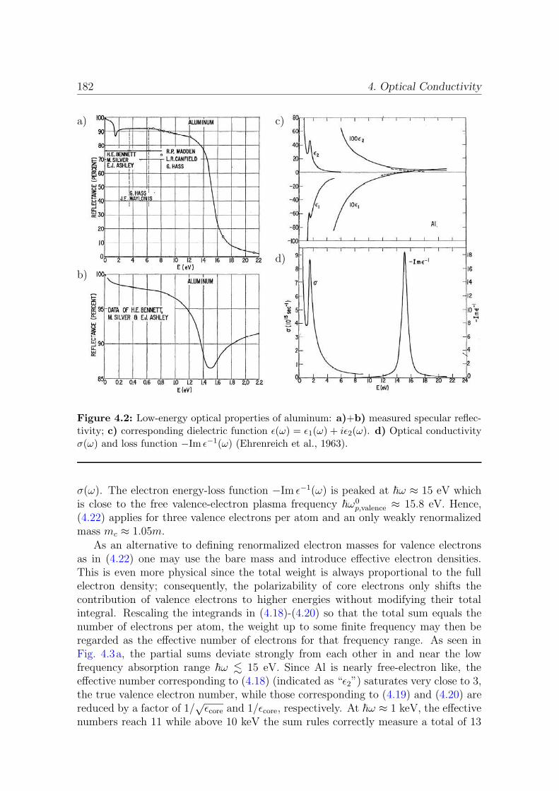
182 4. Optical Conductivity
a)
b)
c)
d)
Figure 4.2: Low-energy optical properties of aluminum: a)+b) measured specular reflec-tivity; c) corresponding dielectric function ε(ω) = ε1(ω) + iε2(ω). d) Optical conductivityσ(ω) and loss function −Im ε−1(ω) (Ehrenreich et al., 1963).
σ(ω). The electron energy-loss function −Im ε−1(ω) is peaked at ~ω ≈ 15 eV whichis close to the free valence-electron plasma frequency ~ω0
p,valence ≈ 15.8 eV. Hence,(4.22) applies for three valence electrons per atom and an only weakly renormalizedmass mc ≈ 1.05m.
As an alternative to defining renormalized electron masses for valence electronsas in (4.22) one may use the bare mass and introduce effective electron densities.This is even more physical since the total weight is always proportional to the fullelectron density; consequently, the polarizability of core electrons only shifts thecontribution of valence electrons to higher energies without modifying their totalintegral. Rescaling the integrands in (4.18)-(4.20) so that the total sum equals thenumber of electrons per atom, the weight up to some finite frequency may then beregarded as the effective number of electrons for that frequency range. As seen inFig. 4.3a, the partial sums deviate strongly from each other in and near the lowfrequency absorption range ~ω . 15 eV. Since Al is nearly free-electron like, theeffective number corresponding to (4.18) (indicated as “ε2”) saturates very close to 3,the true valence electron number, while those corresponding to (4.19) and (4.20) arereduced by a factor of 1/
√εcore and 1/εcore, respectively. At ~ω ≈ 1 keV, the effective
numbers reach 11 while above 10 keV the sum rules correctly measure a total of 13
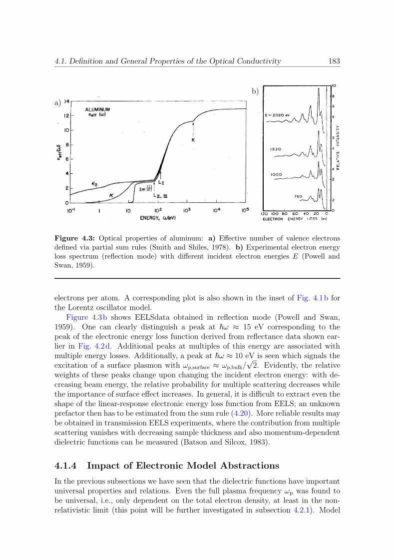
4.1. Definition and General Properties of the Optical Conductivity 183
a)
b)
Figure 4.3: Optical properties of aluminum: a) Effective number of valence electronsdefined via partial sum rules (Smith and Shiles, 1978). b) Experimental electron energyloss spectrum (reflection mode) with different incident electron energies E (Powell andSwan, 1959).
electrons per atom. A corresponding plot is also shown in the inset of Fig. 4.1b forthe Lorentz oscillator model.
Figure 4.3b shows EELSdata obtained in reflection mode (Powell and Swan,1959). One can clearly distinguish a peak at ~ω ≈ 15 eV corresponding to thepeak of the electronic energy loss function derived from reflectance data shown ear-lier in Fig. 4.2d. Additional peaks at multiples of this energy are associated withmultiple energy losses. Additionally, a peak at ~ω ≈ 10 eV is seen which signals theexcitation of a surface plasmon with ωp,surface ≈ ωp,bulk/
√2. Evidently, the relative
weights of these peaks change upon changing the incident electron energy: with de-creasing beam energy, the relative probability for multiple scattering decreases whilethe importance of surface effect increases. In general, it is difficult to extract even theshape of the linear-response electronic energy loss function from EELS; an unknownprefactor then has to be estimated from the sum rule (4.20). More reliable results maybe obtained in transmission EELS experiments, where the contribution from multiplescattering vanishes with decreasing sample thickness and also momentum-dependentdielectric functions can be measured (Batson and Silcox, 1983).
4.1.4 Impact of Electronic Model Abstractions
In the previous subsections we have seen that the dielectric functions have importantuniversal properties and relations. Even the full plasma frequency ωp was found tobe universal, i.e., only dependent on the total electron density, at least in the non-relativistic limit (this point will be further investigated in subsection 4.2.1). Model
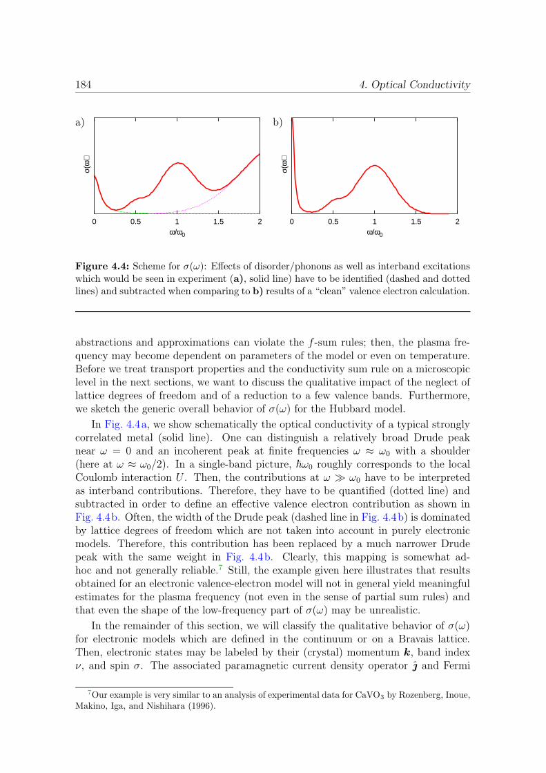
184 4. Optical Conductivity
0 0.5 1 1.5 2
σ(ω
)
ω/ω0
0 0.5 1 1.5 2
σ(ω
)
ω/ω0
a) b)
Figure 4.4: Scheme for σ(ω): Effects of disorder/phonons as well as interband excitationswhich would be seen in experiment (a), solid line) have to be identified (dashed and dottedlines) and subtracted when comparing to b) results of a “clean” valence electron calculation.
abstractions and approximations can violate the f -sum rules; then, the plasma fre-quency may become dependent on parameters of the model or even on temperature.Before we treat transport properties and the conductivity sum rule on a microscopiclevel in the next sections, we want to discuss the qualitative impact of the neglect oflattice degrees of freedom and of a reduction to a few valence bands. Furthermore,we sketch the generic overall behavior of σ(ω) for the Hubbard model.
In Fig. 4.4a, we show schematically the optical conductivity of a typical stronglycorrelated metal (solid line). One can distinguish a relatively broad Drude peaknear ω = 0 and an incoherent peak at finite frequencies ω ≈ ω0 with a shoulder(here at ω ≈ ω0/2). In a single-band picture, ~ω0 roughly corresponds to the localCoulomb interaction U . Then, the contributions at ω À ω0 have to be interpretedas interband contributions. Therefore, they have to be quantified (dotted line) andsubtracted in order to define an effective valence electron contribution as shown inFig. 4.4b. Often, the width of the Drude peak (dashed line in Fig. 4.4b) is dominatedby lattice degrees of freedom which are not taken into account in purely electronicmodels. Therefore, this contribution has been replaced by a much narrower Drudepeak with the same weight in Fig. 4.4b. Clearly, this mapping is somewhat ad-hoc and not generally reliable.7 Still, the example given here illustrates that resultsobtained for an electronic valence-electron model will not in general yield meaningfulestimates for the plasma frequency (not even in the sense of partial sum rules) andthat even the shape of the low-frequency part of σ(ω) may be unrealistic.
In the remainder of this section, we will classify the qualitative behavior of σ(ω)for electronic models which are defined in the continuum or on a Bravais lattice.Then, electronic states may be labeled by their (crystal) momentum k, band indexν, and spin σ. The associated paramagnetic current density operator and Fermi
7Our example is very similar to an analysis of experimental data for CaVO3 by Rozenberg, Inoue,Makino, Iga, and Nishihara (1996).
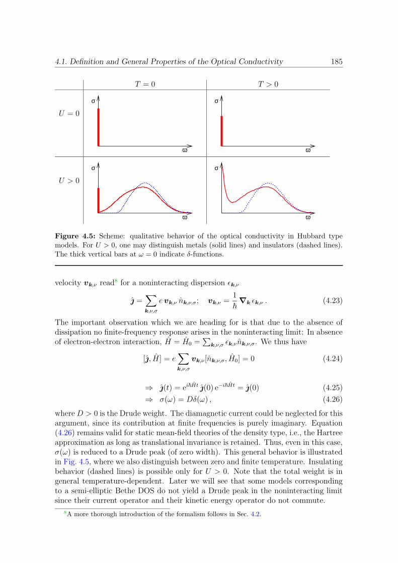
4.1. Definition and General Properties of the Optical Conductivity 185
T = 0 T > 0
U = 0
ω
σ
ω
σ
U > 0
ω
σ
ω
σ
Figure 4.5: Scheme: qualitative behavior of the optical conductivity in Hubbard typemodels. For U > 0, one may distinguish metals (solid lines) and insulators (dashed lines).The thick vertical bars at ω = 0 indicate δ-functions.
velocity vk,ν read8 for a noninteracting dispersion εk,ν
=∑
k,ν,σ
evk,ν nk,ν,σ; vk,ν =1
~∇k εk,ν . (4.23)
The important observation which we are heading for is that due to the absence ofdissipation no finite-frequency response arises in the noninteracting limit: In absenceof electron-electron interaction, H = H0 =
∑
k,ν,σ εk,νnk,ν,σ. We thus have
[, H] = e∑
k,ν,σ
vk,ν [nk,ν,σ, H0] = 0 (4.24)
⇒ (t) = ei~Ht (0) e−i~Ht = (0) (4.25)
⇒ σ(ω) = Dδ(ω) , (4.26)
whereD > 0 is the Drude weight. The diamagnetic current could be neglected for thisargument, since its contribution at finite frequencies is purely imaginary. Equation(4.26) remains valid for static mean-field theories of the density type, i.e., the Hartreeapproximation as long as translational invariance is retained. Thus, even in this case,σ(ω) is reduced to a Drude peak (of zero width). This general behavior is illustratedin Fig. 4.5, where we also distinguish between zero and finite temperature. Insulatingbehavior (dashed lines) is possible only for U > 0. Note that the total weight is ingeneral temperature-dependent. Later we will see that some models correspondingto a semi-elliptic Bethe DOS do not yield a Drude peak in the noninteracting limitsince their current operator and their kinetic energy operator do not commute.
8A more thorough introduction of the formalism follows in Sec. 4.2.
186 4. Optical Conductivity
4.2 Kubo Formalism
In this section, we will discuss the formalism leading to expressions for σ(ω) both inthe continuum and on the lattice in enough detail to expose the microscopic originand ranges of validity of sum rules.
4.2.1 Kubo Formalism in the Continuum
As reviewed in App. D.1, the interaction of a particle at position r with charge qwith an external time varying electric field may be fully described in terms of a shiftof its momentum by qA(r)/c, where A(r) is the vector potential. Furthermore,within the Coulomb gauge, the electrical interaction between charged particles isinstantaneous. In the nonrelativistic limit, we can, thus, assume the following first-quantized electronic Hamiltonian for a number of Ne electrons,9
H = Hint(r1, r2, . . . , rNe) +
Ne∑
i=1
1
2m
(
pi −e
cA(ri, t)
)2
. (4.27)
Here, the interaction Hamiltonian Hint may contain arbitrary interactions of electronswith a (static) lattice potential as well as electron-electron interactions. This term willenter the results only implicitly via its influence on the eigenstates of the unperturbedsystem and their occupation in the thermal ensemble. From (4.27) and vi = ∇pi
Hwe can read off the total current,
∫
dr J(r, t) =Ne∑
i=1
evi =Ne∑
i=1
e
m
(
pi −e
cA(ri)
)
. (4.28)
In (4.28), we may distinguish a diamagnetic contribution −∑Ne
i=1e2
mcA(ri) from the
paramagnetic current, the density of which reads in symmetrized form,10
j(r, t) =e
2m
Ne∑
i=1
(piδ(r − ri) + δ(r − ri)pi
). (4.29)
Denoting the thermal expectation value11 of some observable O in the presence ofthe vector potential by 〈O〉A, the current density is, thus, exactly given by
〈J(r, t)〉A = 〈j(r, t)〉A −e2
mcA(r, t)〈n(r, t)〉A . (4.30)
Since we only need the linear response current, i.e., contributions to J which are atmost linear in A, we can take the density expectation value in (4.30) in zeroth or-
der. In the long-wavelength limit, the diamagnetic contribution is then − e2n0
mcA(r, t),
9Note that following the usual convention the electron charge is here denoted as e, not −e.10Here and in the following, we use the upper-case symbol J for the total current and the lower-
case symbol j for the paramagnetic current or its density.11Due to the explicit time dependence of H, we here have to use a generalized definition of the
thermal average in terms of a time-dependent density operator ρ(t); see App. D.2.
4.2. Kubo Formalism 187
where n0 is the average density. The remaining problem is the calculation of 〈j(r, t)〉Ain linear order in A. For this purpose, it suffices to consider the linear perturbingpart of the Hamiltonian12 which may be expressed as
H ′(t) = −1
c
∫
dr j(r, t) ·A(r, t) . (4.31)
From (D.2) we have for periodic field E(r, t) = Eqei(q·r−ωt)
A(r, t) = − icω
E(r, t) . (4.32)
Thus, we can write, switching to second quantized notation (with V denoting thetotal volume),
H ′(t) = −Vc
−q(t) ·Aq(t) =iV
ω−q(t) ·Eqe
−iωt . (4.33)
Using (D.21) and assuming that the response is restricted to the same wave vectoras the perturbing field, i.e., for not too short wavelengths, the paramagnetic linearresponse current reads (denoting directions as α or β),
〈q,α(ω)〉A = − iV
ω + i0+Eq,β(ω) 〈〈q,α, −q,β 〉〉(ω + i0+) (4.34)
From (4.4), (4.30), and (D.22) we get the general expression for continuum systems13
σαβ(q, ω) =V
~(ω + i0+)
∞∫
0
dt ei(ω+i0+)t〈[†q,α(t), q,β(0)]〉+ in0e
2
m(ω + i0+)δαβ (4.35)
Here, the time dependence of the operator is in the interaction picture (see Sec. D.2)and the long wavelength limit has been used to replace n(r, t) by the average densityn0. In the optical limit q → 0, the current density operator = † is hermitian. Forsystems with cubic symmetry, the current flow in perpendicular directions is thenuncorrelated and σαβ(0, ω) reduces to the scalar σ(ω). Equation (4.35) is correctboth for T = 0 (then the outer brackets indicate the ground state expectation value)and for T > 0 (when the brackets imply thermal averaging) and for longitudinal aswell as transverse electric fields.
Since the susceptibility, i.e., the integral in (4.35) falls off as 1/ω or faster [cf.(D.25)], the high-frequency limit of σ(ω) is determined by the second, diamagneticterm which is proportional to the squared free plasma frequency ω2
p = 4πn0e2/m.
Thus, the frequency sum (4.19) is unchanged by the interactions of electrons, bothwith the lattice ions and among themselves,
∞∫
0
dωRe σαβ(ω) =1
2
∞∫
−∞
dωn0e
2
mπδ(ω) δαβ =
ω2p
8δαβ (4.36)
12Note that the quadratic term in H had to be considered for deriving the correct expression forthe full current.
13Note that (4.35) is valid in Gaussian units. For SI units, its right hand side has to be dividedby 4πε0.
188 4. Optical Conductivity
In the noninteracting limit, where correlations vanish, Re σ(ω) reduces to the dia-magnetic δ-function contributions. Interactions shift weight from ω = 0 to finitefrequencies without changing the total weight. Thus, the full universal f -sum ruleis indeed found to be valid, at least within the (zeroth order) Born-Oppenheimerapproximation and in the limit that optical absorption decays below a cutoff energyE with E
~c¿ π
a.
4.2.2 Kubo Formalism on a Lattice
In Wannier representation, the vector potential can be treated (Kohn, 1964; Shastryand Sutherland, 1990; Scalapino, White, and Zhang, 1992; Dagotto, 1994) by a gaugetransformation of the Wannier wave functions Φl(r) centered at site Rl,
Φl(r) 7→ Φl(r, t) =
[
exp
(
ie
c~
Rl∫
R0
dr ·A(r′, t)
)]
Φi(r), (4.37)
where the free choice of R0 determines the arbitrary overall phase factor. In thelong-wavelength limit q → 0, the vector potential can be taken out of the integral.Then, the change in the Hamiltonian consists of multiplying the hopping elementsdefined in (1.10) by so-called Peierls phase factors,14
tij = t0ij exp(
−i ec~
(Ri −Rj) ·A)
. (4.38)
Note that only hopping elements with components parallel to the vector field Aare modified. In comparing (4.38) with (D.3) we identify the additional factor asexp(−i∆S/~), where ∆S is the field contribution to the action for the world lineconnecting the lattice sites in absence of a scalar potential φ.
Before considering the general case, we specialize on the more commonly treatedcase of the hypercubic tight-binding model with nearest-neighbor hopping, where theunperturbed kinetic energy is given by K0 = −t∑〈ij〉,σ
(c†iσ cjσ + c†jσ ciσ
). Expanding
the phase factors to lowest orders in A,15 we obtain the modified kinetic energy:
K = K0 +d∑
α=1
(− V
cαAα +
e2a2
2~2c2K0αA
2α + . . .
)(4.39)
where the lattice paramagnetic current density operator and the kinetic energy in
14While, in general, the interaction matrix elements defined in (1.11) also acquire Peierls phases,on-site elements and intersite contributions of the density-density type remain unchanged.
15We need quadratic order in order to retain the linear contribution to the current operator, Jα.
4.2. Kubo Formalism 189
direction α are given by (lattice constant a)16
α = − ietaV ~
∑
i,σ
(
c†iσ ci+eασ− c†i+eασ
ciσ
)
, (4.40)
K0α = −t
∑
i,σ
(
c†iσ ci+eασ+ c†i+eασ
ciσ
)
. (4.41)
The full current density operator is obtained by variation of K with respect to thevector potential (Scalapino et al., 1992),
Jα = − c
V
δK
δAα= α +
e2a2
V c~2K0αAα. (4.42)
As in the continuum case, the conductivity can be expressed in terms of a correlationfunction and of the diamagnetic contribution,
σαα(ω) =iV
ω〈〈α, α〉〉(ω + i0+)− i e2a2
V ~2(ω + i0+)〈K0
α〉 (4.43)
Evidently, the reduction to a single-band model has changed the diamagnetic contri-bution and, consequently, the sum-rule to a nonuniversal form. For the assumptionused in deriving (4.43) of nearest-neighbor hopping on a hypercubic lattice, the fre-quency sum is seen to be proportional to the kinetic energy,
∞∫
0
dω σαα(ω) = −π2
e2a2
V ~2〈K0
α〉 = − πe2
2d~2a2−d 〈K0〉
N. (4.44)
For the more general case of arbitrary hopping on a Bravais lattice, we have toconsider that the phase shift due to the vector potential A increases with hoppingdistance. For later use, we want to obtain expressions in momentum representation.Thus, we assume for the unperturbed Hamiltonian (with band index ν),
H =∑
k,ν,σ
εk,ν nk,ν,σ + Hee
ni,ν,σ
, (4.45)
where the interaction term is of the density-density type.17 Due to inversion symme-try we can always write for a selected lattice direction x,
εk,ν =∞∑
n=1
fν,n(k⊥) cos(naxkx) (4.46)
16Note that for this particular case and up to prefactors, the kinetic energy and the currentoperator are sums over the real and the imaginary part, respectively, of the same bond hoppingoperator.
17Note that, in contrast to the continuum formulation, the restriction to density-density typeinteraction terms is in general a serious approximation in the Wannier representation; see subsection1.1.3.
190 4. Optical Conductivity
where k⊥ is the projection of k on directions perpendicular to ex. Since the nth
term in (4.46) contains hopping to nth-nearest neighbors, we can use straightforwardgeneralizations of (4.39) and (4.42) to find for the paramagnetic current densityoperator x and diamagnetic current density operator dia
x , respectively,
x = −eaxV ~
∑
k,ν,σ
nk,ν,σ
∞∑
n=1
nfν,n(k⊥) sin(nkx) =e
V ~
∑
k,ν,σ
nk,ν,σ∂
∂kxεk,ν (4.47)
diax =
e2A
V c~2
∑
k,ν,σ
nk,ν,σ∂2
∂k2x
εk,ν (4.48)
We, thus, obtain for the conductivity,
σαα(ω) =ie2
V ~2(ω + i0+)
∑
ν,ν′,σ,σ′
∑
k,k′
vk,ν,αvk′,ν′,α〈〈nk,ν,σ, nk′,ν′,σ′ 〉〉(ω + i0+)
+ie2
V ~2(ω + i0+)
∑
k,ν,σ
〈nk,ν,σ〉∂2
∂k2α
εk,ν ,
(4.49)
where vk,ν,α = ∂∂kα
εk,ν is the α component of the Fermi velocity of band ν for mo-mentum k. Consequently, the f -sum rule reads
∞∫
0
dω σαα(ω) =πe2
2V ~2
∑
k,ν,σ
〈nk,ν,σ〉∂2
∂k2α
εk,ν . (4.50)
For a full electronic model, we can use the free dispersion for a single band with∂2εk∂k2 = ~
2
mwhich leads to the free diamagnetic term and, thus, to the free sum rule
(4.21), i.e.,∫
dω σαα(ω) =ω2
p
8with ω2
p = 4πne2
m.
4.2.3 General Confirmation of the f-sum Rule
While the fact that the paramagnetic current will not contribute to the f -sum rulefollows on quite general grounds from (D.25), we can drop the condition of a boundedspectrum used in Sec. D.2. In the course of re-deriving the sum rule (4.50), we will alsoidentify a contribution to the paramagnetic current which cancels the diamagneticcurrent. In this subsection, only the single-band case is considered explicitly.
For the Hamiltonian (4.45), the polarization operator P =∑
i rini commuteswith the interaction term
[Hee, P ] =∑
i
ri[Hee, ni] = 0 . (4.51)
and can be used for expressing the current density operators:
α =e
V
d
dtPα = − ie
V ~[Pα, K] (4.52)
diaα =
e2A
V c~2[Pα, [Pα, K]] . (4.53)
4.2. Kubo Formalism 191
Thus, we can rewrite the current-current correlation function,
〈〈α, α〉〉(ω) =ie
V ~
∞∫
0
dt eiωt〈[ d
dtPα(t), α(0)]〉 (4.54)
=ie
V ~
(
eiωt〈[Pα(t), α(0)]〉∣∣∞0−
∞∫
0
dt (iω)eiωt〈[Pα(t), α(0)]〉)
(4.55)
= − ie
V ~〈[Pα, α]〉+
e ω
V ~
∞∫
0
dt eiωt〈[Pα(t), α]〉 (4.56)
The operator in the first term, − ieV ~
[Pα, α] = − e2
V 2~2 [Pα, [Pα, K]], cancels the diamag-netic contribution to σαα(ω). Thus, the f -sum reads,18
∞∫
0
dωReσαα(ω) =1
2
ie
~
∞∫
0
dt 2πδ(t)〈[Pα(t), α]〉 (4.57)
=πe2
2V ~2〈[Pα, [Pα, K]]〉 , (4.58)
which reduces to (4.50) since [Pα, [Pα, K]] =∑
k,σ nk,σd2
dk2αεk.
From (4.56), we can also express the total optical conductivity as
σαα(ω) = e〈〈Pα, α〉〉(ω) . (4.59)
This form makes the qualitative behavior seen in Fig. 4.5 physically plausible: Inthe presence of (small) interactions, quasiparticles acquire a finite lifetime and, thus,correlations generically decay in real time which leads to σ(ω) being finite (i.e., notinfinite) at all ω. At T = 0, however, quasiparticles directly at the Fermi surfaceare still stable and may give rise to a (reduced) Drude δ-peak. Within Fermi liquidtheory, the reduction factor is Z, the quasiparticle weight. At finite T , all lifetimesare finite (but still large near the Fermi surface) so that the Drude peak broadens withincreasing interaction until both Fermi liquid theory breaks down and the Drude peakmay disappear in the incoherent background or vanish when a gap opens. Assuming,on the other hand, that σ(ω) remains finite at all ω, one can as well work with thereal part of the paramagnetic contribution for ω > 0 as given by (4.49) and obtainσdc as limω→0 σ(ω). In fact, in numerical calculations at T = 0 the Drude weight isoften obtained via the f -sum rule (Dagotto, 1994).
18Strictly speaking, the integral on the right hand side of (4.57) is undefined. For a more rig-orous proof, one needs to keep a “small” real η > 0, use Re
∫∞
0dωeiω(t+iη) = η/(η2 + t2) and
the fact that Im 〈i[A, B]〉 = 0 for Hermitian operators A, B. Then, (4.58) can be derived fromlimη→0 Re
∫∞
0dω
∫∞
0dteiω(t+iη)f(t) = f(0+) limη→0
∫∞
0dtη/(η2 + t2) = f(0+)π/2 for a real function
f(t).
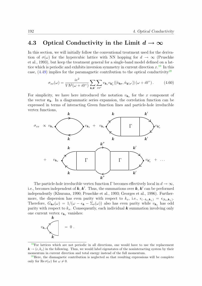
192 4. Optical Conductivity
4.3 Optical Conductivity in the Limit d → ∞
In this section, we will initially follow the conventional treatment used for the deriva-tion of σ(ω) for the hypercubic lattice with NN hopping for d → ∞ (Pruschkeet al., 1993), but keep the treatment general for a single-band model defined on a lat-tice which is periodic and exhibits inversion symmetry in current direction x.19 In thiscase, (4.49) implies for the paramagnetic contribution to the optical conductivity20
σxx(ω) =ie2
V ~2(ω + i0+)
∑
k,k′
∑
σσ′
vkxvk′
x〈〈nkσ, nk′σ′ 〉〉(ω + i0+) . (4.60)
For simplicity, we have here introduced the notation vkxfor the x component of
the vector vk. In a diagrammatic series expansion, the correlation function can beexpressed in terms of interacting Green function lines and particle-hole irreduciblevertex functions,
σxx ∝ vkx
k
k
vkx+ vkx Γ
k
k
k′
k′
vk′x
+ vkx
k
k
Γ
k′′
k′′
Γ
k′
k′
vk′x
+ . . .
The particle-hole irreducible vertex function Γ becomes effectively local in d→∞,i.e., becomes independent of k, k′. Thus, the summations over k, k′ can be performedindependently (Khurana, 1990; Pruschke et al., 1993; Georges et al., 1996). Further-more, the dispersion has even parity with respect to kx, i.e., ε(−kx,k⊥) = ε(kx,k⊥).Therefore, Gkσ(ω) = 1/(ω − εk − Σσ(ω)) also has even parity while vkx
has oddparity with respect to kx. Consequently, each individual k summation involving onlyone current vertex vkx
vanishes:
vkx
k
k
= 0 .
19For lattices which are not periodic in all directions, one would have to use the replacementk→ (ε, kx) in the following. Thus, we would label eigenstates of the noninteracting system by theirmomentum in current direction and total energy instead of the full momentum.
20Here, the diamagnetic contribution is neglected so that resulting expressions will be completeonly for Reσ(ω) for ω 6= 0.

4.3. Optical Conductivity in the Limit d→∞ 193
Thus, vertex corrections do not contribute in d → ∞ and (4.60) reduces to thebubble contribution (with inverse temperature β and Matsubara frequencies iωn)
σxx(iν) =e2
V ~2νT∑
k,σ,ωn
v2kxGkσ(iωn)Gkσ(iωn + iν) . (4.61)
The momentum independence21 of Σ(ω) can now be used for replacing the momentumsum by an energy integral (where N denotes number of sites)
σxx(iν) = 2e2
~2ν
N
V
∞∫
−∞
dε ρxx(ε)T∑
n
Gε(iωn)Gε(iωn + iν) . (4.62)
Here, we have introduced [cf. (3.11)]
Gε(iωn) ≡ Gεk,σ(iωn) =1
iωn − εk − Σσ(iωn)(4.63)
and
ρxx(ε) :=1
N
∑
k
v2kxδ(ε− εk) . (4.64)
and specialized on the paramagnetic case. The factor of 2 in (4.62) is for spin degen-eracy. Note that ρxx(ε) = O(1/d); in the isotropic case, we have dρxx(ε) = ρ(ε) :=1N
∑
k |vk|2δ(ε− εk). Analytic continuation of (4.62) yields
Re σxx(ω) = σ0
∞∫
−∞
dε ρxx(ε)
∞∫
−∞
dω′Aε(ω′)Aε(ω
′ + ω)nf(ω
′)− nf(ω + ω′)
ω, (4.65)
where
Aε(ω) = − 1
πImGε(ω) , nf(ω) =
(1 + eβ(ω−µ)
)−1, (4.66)
and
σ0 :=2πe2
~2
N
V. (4.67)
We note that the limit of infinite dimensionality enters (4.65) only via the localityof the self-energy and of the irreducible vertex function. Using both properties asan approximation, (4.65) may therefore also be applied in finite dimensions. Fornumerical results, we will set e, ~, and the lattice spacing a to unity which correspondsto σ0 = 2π.
21If Σ(ω) was momentum-dependent, the momentum sum in the general bubble-sum expression(4.61) could not be replaced by an energy integral. For piecewise constant Σ(ω) like in the DCA,however, a generalization of (4.152) could be applied on each patch. The individual contributionsfor each value of the coarse-grained momentum would then have to be summed up for the totaloptical conductivity.
194 4. Optical Conductivity
4.3.1 Optical Conductivity for the Hypercubic Lattice
For a hypercubic lattice with NN hopping, ρxx(ε) is proportional to the DOS,
ρhcxx(ε) =
t∗2a2
dρhc(ε) (4.68)
We will here first reproduce Pruschke et al.’s (1993) proof using the same Fouriertransform technique that had been used before for calculating the (Gaussian) DOSof the hc lattice (Muller-Hartmann, 1989a) and then derive a shorter version which ismore general. Using εk = −2t
∑dα=1 cos(kα) and ∂εk
∂kα= 2t sin(kα), which corresponds
to lattice spacing a = 1, ρhcxx(ε) transforms as follows,
∞∫
−∞
dε ρxx(ε) eisε =
[ π∫
−π
dk
2πe−2ist cos(k)
]d−1 [π∫
−π
dk
2π4t2 sin2(k)e−2ist cos(k)
]
(4.69)
= 2t2[J0(2st)
]d(
1 +J2(2st)
J0(2st)
)
(4.70)
= 2t2 exp
[
d ln(
1− (2st)2
4+ · · ·
)
+ ln(
1 +(2st)2
8+ · · ·
)]
= 2t2 exp
[
−(st∗)2
2+O(
1
d)
]
. (4.71)
Keeping only leading terms, transforming back, and determining the dependence ona from scaling, one obtains (using Z = 2d)
ρxx(ε) = 2t2a2ρ(ε) , (4.72)
which confirms (4.68). Thus, the conductivity reads,
Re σhcxx(ω) =
2πe2a2t∗2
d~2
N
V
∞∫
−∞
dε ρ(ε)
×∞∫
−∞
dω′Aε(ω′)Aε(ω
′ + ω)nf(ω
′)− nf(ω + ω′)
ω.
(4.73)
While the above approach using Bessel functions Jν(x) has the advantage that itallows for the calculation of corrections terms of O(1/d) and beyond, the d → ∞result can be obtained more directly: Let us assume that the total noninteractingkinetic energy separates into a contribution depending only on hopping in the currentdirection and a contribution which does not involve hopping in that direction andthat the latter contribution dominates the bandwidth,
εk = ε⊥k⊥+ εxkx
,
√
〈(εxkx− 〈εxkx
〉)2〉√
〈(εk − 〈εk〉)2〉= O(1/d) . (4.74)

4.3. Optical Conductivity in the Limit d→∞ 195
Then, to leading order,
ρxx(ε) =1
N
∑
k
v2kxδ(ε− ε⊥k⊥
) = ρ(ε)ax2π
π/ax∫
−π/ax
dkx v2kx. (4.75)
Thus, expression (4.73) directly applies to all stacked lattices in d → ∞ when hop-ping in current direction (lattice spacing ax) is restricted to nearest neighbors withamplitude t∗/
√Z. The suitable generalization for arbitrary-range hopping in current
direction follows from (4.75). Note that the definition of hopping elements in cur-rent direction does not impact any local properties and that the frequency sum overσxx(ω) will be directly related to local properties (such as the kinetic energy) onlyfor isotropic models.
4.3.2 f-sum Rule within the DMFT
In this subsection, we will derive a very general new form of the f -sum rule for theoptical conductivity which applies to all cases where expression (4.65) for σ(ω) isused, in particular to d = ∞. We do not need to make any assumptions about thefunctional form of ρxx(ε) other than that it has to be piecewise differentiable. Inparticular, we do not need to know the dispersion εk; thus, our results can even beapplied to lattices without (full) k-space. Furthermore, we can show that the sumrule is fulfilled also for approximate DMFT solutions as long as the self-energy iscausal. Finally, we present an efficient computation scheme for the frequency sumdirectly on the imaginary axis.
We start with the noninteracting limit. Then the spectral function becomes aδ-function, Aε(ω)→ δ(ω − ε), and we obtain from (4.65) [with σ0 defined in (4.67)],
∞∫
0
dω σxx(ω) =σ0
2
∞∫
−∞
dε ρxx(ε)
∞∫
−∞
dω
∞∫
−∞
dω′ δ(ω′ − ε)δ(ω + ω′ − ε)nf(ω′)− nf(ω
′ + ω)
ω
= −σ0
2
∞∫
−∞
dε ρxx(ε)d
dεnf(ε) =
σ0
2
∞∫
−∞
dε ρ′xx(ε)nf(ε) (4.76)
=σ0
4
⟨ ρ′xx(ε)
ρ(ε)
⟩. (4.77)
Here and in the following, the prime denotes the derivative with respect to the argu-ment, ρ′xx(ε) := d
dερxx(ε). No boundary terms arise in the partial integration in (4.76)
since ρ(ε) vanishes at the band edges. We further introduced the notation
〈f(ε)〉 :=
∞∫
−∞
dε ρ(ε) (nε,↑ + nε,↓) f(ε) , (4.78)
where the expectation value of the generalized momentum distribution function is forarbitrary interaction given in terms of Fermi distribution function nf(ω), chemical

196 4. Optical Conductivity
potential µ, and spectral function Aε,σ(ω) by
nε,σ := 〈nε,σ〉 =
∞∫
−∞
dω nf(ω − µ)Aε,σ(ω) . (4.79)
In the paramagnetic case, nε ≡ nε,σ. While the expression (4.77) was derived for thenoninteracting limit, and, thus, explicitly only determines the weight of the Drudepeak, one might suspect that it remains valid in connection with (4.79) in the in-teracting case. This would amount to a generalization of the hc sum rule (4.44),where (for t∗ = 1 and a = 1), ρ(ε) = ρ(ε) = e−ε
2/2 and 〈ρ′(ε)/ρ(ε)〉 = 〈−ε〉 is minusthe kinetic energy. For a proof of (4.77) in the general case, we will show that thefrequency dependent part in (4.65), denoted as I(ε), sums up to −dnε/dε,
I(ε) =
∞∫
−∞
dω
∞∫
−∞
dω′Aε(ω′)Aε(ω
′ + ω)nf(ω
′)− nf(ω′ + ω)
ω(4.80)
=
∞∫
−∞
dω′′∞∫
−∞
dω′Aε(ω′)Aε(ω
′′)nf(ω
′)− nf(ω′′)
ω′′ − ω′ (4.81)
=
∞∫
−∞
dω′ nf(ω′)Aε(ω
′)
∞∫
−∞
dω′′ Aε(ω′′)
ω′′ − ω′
+
∞∫
−∞
dω′′ nf(ω′′)Aε(ω
′′)
∞∫
−∞
dω′ Aε(ω′)
ω′ − ω′′ (4.82)
=2
π
∞∫
−∞
dω nf(ω) ReGε(ω) ImGε(ω) (4.83)
= − 1
π
∞∫
−∞
dω nf(ω)d
dε
Im Σ(ω)
(ω − ε− Re Σ(ω))2 + Im Σ(ω)2(4.84)
= − d
dεnε . (4.85)
Thus, the f -sum rule for the optical conductivity within the DMFT, i.e., withinthe bubble approximation with a k-independent self-energy reads
∞∫
0
dω σxx(ω) =σ0
2
∞∫
−∞
dε ρxx(ε)(
− dnεdε
)
(4.86)
=σ0
2
∞∫
−∞
dε ρ′xx(ε)nε =σ0
4
⟨ ρ′xx(ε)
ρ(ε)
⟩. (4.87)
This sum rule is of great practical value as a check of numerical results. Note that itcannot only be evaluated from real-frequency data, but also directly on the imaginary
4.3. Optical Conductivity in the Limit d→∞ 197
axis, since
− dnεdε
=1
π
∞∫
−∞
dω Im(G2ε(ω)
)nf(ω) = T
∑
n
G2ε(iωn)
= T∑
n
(ε+ Re Σn)2 − (ωn − Im Σn)
2
((ε+ Re Σn)2 + (ωn − Im Σn)2
)2 . (4.88)
Since the terms in (4.88) decay as 1/ω2n, the sum over n does not require additional
convergence factors. Furthermore, due to the fast convergence, the sum is insensitiveto the large-frequency behavior of the self-energy. Since, on the other hand, QMCmethods in general and the particular Fourier-transform techniques used in this workdo not yield good estimates for Σn at large frequencies, the estimate for (4.88) will beeven much better conditioned than, e.g., the estimate (3.10) for the kinetic energy.In fact, we found that computing nε by integrating over dnε/dε as given by (4.88)reduces the ∆τ error for the kinetic energy considerably when compared with thedirect computation (3.10).
4.3.3 f-sum Rule and General Dispersion Formalism
Within the framework of the general dispersion method developed in Sec. 2.3, the fullnoninteracting dispersion εk can be written in terms of the transformation functionF and the dispersion εhc
k of the hypercubic lattice with NN hopping only. Then, thederivatives appearing in (4.47) through (4.50) read
∂εk∂kx
=∂
∂kxF(εhc
k ) = F ′(εhck )∂εhc
k
∂kx(4.89)
and∂2εk∂k2
x
= F ′(εhck )∂2εhc
k
∂k2x
+ F ′′(εhck )
(∂εhc
k
∂kx
)2
. (4.90)
Using (for a = 1)
εhck =
√
2
d
d∑
α=1
cos(kα);∂εhc
k
∂kx= −
√
2
dsin(kx);
∂2εhck
∂k2x
= −√
2
dcos(kx) (4.91)
we can carry out the sum in (4.64)
ρ(ε) = limd→∞
dρxx(ε)
=1
N
∑
k
limd→∞
d(∂εk∂kx
)2
δ(ε− εk)
= limd→∞
d
(2π)d
∫
dkx
∫
dk⊥(F ′(εhc
⊥ (k⊥) + ε‖(kx)))2 2
dsin2(kx)
× δ(ε−F
(εhc⊥ (k⊥) + ε‖(kx)
))
=
[
limd→∞
1
(2π)d−1
∫
dk⊥(F ′ (εhc
⊥ (k⊥)))2
δ(ε−F
(εhc⊥))]
1
2π
∫
dkx 2 sin2(kx)
= ρ(ε)(F ′(F−1(ε)
)2, (4.92)
198 4. Optical Conductivity
where we have exploited the fact that the energy of the hypercubic lattice separatesinto contributions depending on kx and on components of k perpendicular to the xdirection, respectively. Since the former is of order 1/d it could be neglected in thefourth line of (4.92). In an analogous fashion one can compute the sum in (4.50)
limd→∞
∑
k,σ
〈nk〉 d∂2εk∂k2
x
= 2
∞∫
−∞
dε ρ(ε)[F ′′(F−1(ε))−F ′(F−1(ε))F−1(ε)
]〈nε〉 (4.93)
Finally, since ρ′(ε) is related with the second derivative of the dispersion,
d
dερ(ε) =
d
dε
((F ′(F−1(ε)
))2ρ(ε)
)
=d
dε
(F ′(F−1(ε)
)ρhc(F−1(ε)
))
= F ′(F−1(ε)) (ρhc)′(F−1(ε)
) (F−1(ε)
)′
+F ′′(F−1(ε)) (F−1(ε)
)′ρhc(F−1(ε)
)
=(ρhc)′(F−1(ε)
)+F ′′(F−1(ε)
)
F ′(F−1(ε)
) ρhc(F−1(ε)
)
=[F ′′(F−1(ε)
)−F−1(ε)F ′(F−1(ε)
)]ρ(ε) (4.94)
we can reformulate the general DMFT sum rule (4.87) in terms of the dispersion:
∞∫
0
dω σxx(ω)(4.87)
=σ0
4d
⟨ ρ′(ε)
ρ(ε)
⟩
(4.94)=
σ0
4d
⟨F ′′(F−1(ε)
)−F−1(ε)F ′(F−1(ε)
)⟩
(4.93)=
σ0
4
∑
k,σ
〈nkσ〉∂2εk∂k2
x
.
(4.95)
Since (4.95) is equivalent to (4.50) for a single band, we have demonstrated theconsistency of our formalism.
4.4 Optical Conductivity for the Bethe Lattice
As discussed in Sec. 2.2, the Bethe “lattice” is more accurately labeled as a tree (aspecial planar graph) since it is does not constitute a regular lattice. In fact, theperiodicity of a regular lattice and the associated graph formed by, e.g., its nearest-neighbor bonds generally imply the existence of an infinite number of inequivalentloops for Z > 2 while the Bethe “lattice” is defined by the complete absence ofloops (and a constant number of nearest neighbors relative to each site). Due to itsdefinition in topological terms only, concepts like directions, angles, and distances
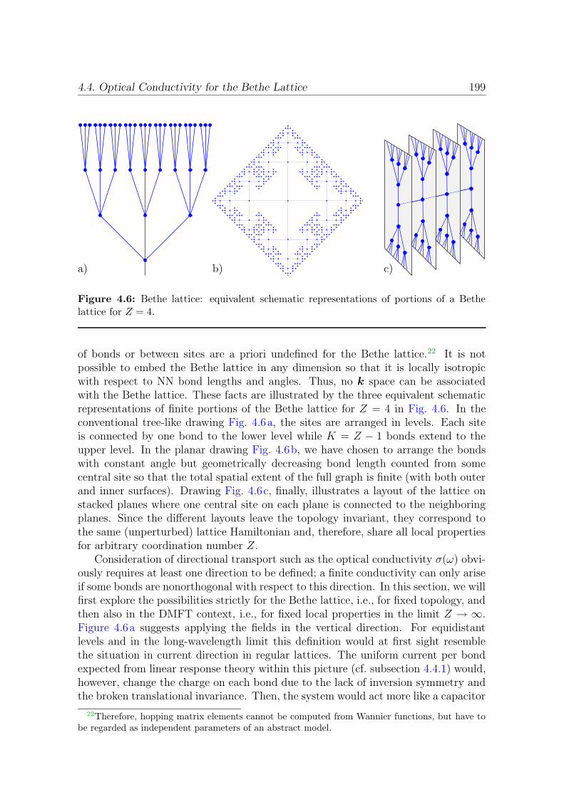
4.4. Optical Conductivity for the Bethe Lattice 199
a) b) c)
Figure 4.6: Bethe lattice: equivalent schematic representations of portions of a Bethelattice for Z = 4.
of bonds or between sites are a priori undefined for the Bethe lattice.22 It is notpossible to embed the Bethe lattice in any dimension so that it is locally isotropicwith respect to NN bond lengths and angles. Thus, no k space can be associatedwith the Bethe lattice. These facts are illustrated by the three equivalent schematicrepresentations of finite portions of the Bethe lattice for Z = 4 in Fig. 4.6. In theconventional tree-like drawing Fig. 4.6a, the sites are arranged in levels. Each siteis connected by one bond to the lower level while K = Z − 1 bonds extend to theupper level. In the planar drawing Fig. 4.6b, we have chosen to arrange the bondswith constant angle but geometrically decreasing bond length counted from somecentral site so that the total spatial extent of the full graph is finite (with both outerand inner surfaces). Drawing Fig. 4.6c, finally, illustrates a layout of the lattice onstacked planes where one central site on each plane is connected to the neighboringplanes. Since the different layouts leave the topology invariant, they correspond tothe same (unperturbed) lattice Hamiltonian and, therefore, share all local propertiesfor arbitrary coordination number Z.
Consideration of directional transport such as the optical conductivity σ(ω) obvi-ously requires at least one direction to be defined; a finite conductivity can only ariseif some bonds are nonorthogonal with respect to this direction. In this section, we willfirst explore the possibilities strictly for the Bethe lattice, i.e., for fixed topology, andthen also in the DMFT context, i.e., for fixed local properties in the limit Z → ∞.Figure 4.6a suggests applying the fields in the vertical direction. For equidistantlevels and in the long-wavelength limit this definition would at first sight resemblethe situation in current direction in regular lattices. The uniform current per bondexpected from linear response theory within this picture (cf. subsection 4.4.1) would,however, change the charge on each bond due to the lack of inversion symmetry andthe broken translational invariance. Then, the system would act more like a capacitor
22Therefore, hopping matrix elements cannot be computed from Wannier functions, but have tobe regarded as independent parameters of an abstract model.
200 4. Optical Conductivity
than as a usual conductor. For a uniform current flow, one would have to balanceincoming and outgoing current on each site; in the long-wavelength limit this wouldamount to geometrically reducing the level spacing upward by a factor of 1/(Z − 1)and, consequently, imply a semi-finite lattice. In fact, the latter situation is verysimilar to that depicted in Fig. 4.6b for which any current definition would also seemartificial. In contrast, the layout depicted in Fig. 4.6c is translationally invariant inthe stacking direction so that fields and currents can be unambiguously defined inthis direction. The main drawbacks of this interpretation are that the lattice siteswithin a plane are then no longer equivalent and that the current flow is limited toa single chain of bonds and, thus, does not scale to the thermodynamic limit. Aswe will show below, there is also no Drude peak in the noninteracting limit for thismodel.
Clearly, the pathologies of the Bethe lattice are even worse for transport phe-nomena than for local properties.23 Still, the availability of DMFT data has ledmany researchers to trying to extract meaningful results for transport properties, inparticular σ(ω), as well. Rozenberg et al. (1995) just ignored the difficulties, usedthe formalism valid for the hypercubic lattice, and wrongly stated that the hc f -sum rule (4.44) was still observed (cf. subsection 4.4.3). Freericks found a derivationwithin the “tree level picture” Fig. 4.6a (Freericks and Jarrell, 1995a; Freericks, 2000).Stumpf (1999) discussed σ(ω) for the single-link stacked picture Fig. 4.6c. In con-trast to above approaches, Uhrig and Vlaming (1993) explored the freedom withinthe DMFT of changing terms of O(1/d) in the Hamiltonian and computed σ(ω) forstacked Bethe lattices.
For the remainder of this section, we attempt a systematic and exhaustive dis-cussion of ways of defining and computing σ(ω) consistently on the basis of DMFTcalculations using a semi-elliptic DOS. For each choice, we characterize the generalbehavior of σ(ω) and the specific form of the f -sum rule. Specifically, the derivationsstrictly for the Bethe lattice by Freericks and by Stumpf are discussed in subsection4.4.1 and subsection 4.4.2, respectively. Going beyond the cited work, we point outan inconsistency in the former approach and explain the lack of coherent transportin the latter. Conductivity for stacked lattices is reviewed in a broad context in sub-section 4.4.3. In subsection 4.4.4, we show that full off-diagonal disorder generallyleads to a very similar expression for σ(ω) as the single-link stacked approach byStumpf. Finally, we show that our generalized-dispersion approach for the first timeyields definition and expressions for an isotropic conductivity corresponding to thesemi-elliptic Bethe DOS in subsection 4.4.5.
4.4.1 Treelike Layout of the Bethe Lattice
In this subsection, we will discuss a formalism developed by Freericks which is basedon the treelike layout of the Bethe lattice shown in Fig. 4.6a. Initially, Freericksand coworkers had followed Rozenberg’s approach of computing σ(ω) for the Bethelattice by application of the expression (4.73) derived for the hc lattice (Chung and
23For a discussion of the importance of surface effects, see Sec. 2.2.
4.4. Optical Conductivity for the Bethe Lattice 201
Freericks, 1998b). After noting a numerical violation of the corresponding f -sum rule(4.44), i.e., a lack of proportionality between the integral over σ(ω) and the full kineticenergy, they realized the need for a careful treatment of the linear response formalismapplicable to the Bethe lattice. They proposed (Chung and Freericks, 1998a)24 anapplication of (4.73), but using a DOS multiplied by a nontrivial (squared) Fermivelocity prefactor of the form 〈v2
kx〉(ε) = 4 − ε2, i.e., ρ(ε) = (4 − ε2)ρ(ε). This
prefactor vanishes at the band edges (at ε = ±2) as expected on general physicalgrounds. Furthermore, the proportionality between the f -sum and the total kineticenergy was seen to be reestablished, albeit with an unexpected prefactor 3. Noderivations were published; Freericks did, however, make a sketch of his treatmentavailable privately (Freericks, 2000) which forms the basis of our derivation givenbelow.
Let us first show analytically which sum rule obtains from using the hc decouplingρxx(ε) = 〈v2
kx〉ρ(ε) with ρ(ε) being the semi-elliptic Bethe DOS (and effectively con-
stant 〈v2kx〉). This is easily accomplished using the formalism developed in subsection
4.3.2,
ρxx(ε) = 〈v2kx〉ρ(ε); ρ(ε) =
1
2π
√4− ε2
⇒ d
dερxx(ε) = −〈v2
kx〉 ε2π
(4− ε2
)−1/2(4.96)
⇒∞∫
0
dω σxx(ω) = 〈v2kx〉σ0
4〈 −ε4− ε2 〉 . (4.97)
Evidently, the frequency sum is indeed not proportional to the expectation value ofthe kinetic energy. This fact is not surprising since the proportionality of the f -sumto the kinetic energy is very specific to the hc case as shown in subsection 4.3.1.
The central assumption made by Freericks is that kinetic energy eigenstates canbe written in the following form,25
|ε〉 =∑
x
(γε)x∑
αx
|x, αx〉 . (4.98)
Here, the integer x counts the level number (i.e., is the vertical coordinate in Fig. 4.6a)and αx is an intra-level coordinate, i.e., labels lattice sites within level x. The latteris written with index x since the set of values that the intra-level coordinate can takedepends on x for Z > 2. The factor26 γε takes the role of a phase shift between levelsalthough, as we will see, its absolute value does not in general equal 1. An expressionfor γε in terms of ε is obtained from the eigenvalue equation for the kinetic energy.
24Note that this reference is the published version of the preprint (Chung and Freericks, 1998b).25Our reproduction of the derivation differs considerably in form from the sketch made available
to us (Freericks, 2000). In particular, we found it necessary to introduce indices within the planes.Unless noted, however, the treatments are equivalent.
26In the following, we will also write γxε ≡ (γε)
x where x is still an exponent rather than an index.
202 4. Optical Conductivity
For the kinetic energy, we can write
T = −2t∑
y
∑
αy
c†y,αy
(cy−1,f(αy) +
Z−1∑
i=1
cy+1,g(αy ,i)
), (4.99)
where f(αy) maps onto the intra-level coordinate of the “root” (on level y − 1) ofsite (y, αy) . Conversely, g(αy, i) maps onto the intra-level coordinate of one of the(Z−1) “children” on the higher level of the same site.27 We obtain for the eigenvalueequation
T |ε〉 = −2t∑
x
(γx−1ε + (Z − 1)γx+1
ε
)∑
αx
|x, αx〉 (4.100)
= −2t(γ−1ε + (Z − 1)γε
)|ε〉 . (4.101)
By definition, the coefficient if front of |ε〉 must equal ε; inverting this equation, weobtain
γε =−ε±
√
ε2 − 4(Z − 1)t2
2(Z − 1)t. (4.102)
Expressing the current operator28 in a form analogous to the kinetic energy,
= iet∑
y
∑
αy
c†y,αy
(− cy−1,f(αy) +
Z−1∑
i=1
cy+1,g(αy ,i)
), (4.103)
the associated eigenvalue equation reads,
|ε〉 = iet(− γ−1
ε + (Z − 1)γε)|ε〉 (4.104)
= ±e√
4(Z − 1)t2 − ε2|ε〉 . (4.105)
The requirement that the eigenvalues of have to be real fixes the band edges,|ε| ≤ 2t
√Z − 1.29 The square root in (4.105) is to be interpreted as 〈vkx
〉(ε) whichimplies that in the limit of Z →∞,
ρxx(ε) = (4t∗2 − ε2)ρ(ε) . (4.106)
Applying the general expression (2.24) specifically for the semi-elliptic DOS (for t∗ =1) then leads to
ρxx(ε) =1
2π
(4− ε2
)3/2(4.107)
∞∫
0
dω σxx(ω) =σ0
4〈 ρ
′xx(ε)
ρ(ε)〉 =
σ0
4〈−3ε〉 , (4.108)
27More formally, we can demand that the mapping (y, αy, i)→ (y+ 1, αy+1) ≡ (y+ 1, g(αy, i)) isinjective and that f(g(αy, i)) = αy for all y, αy, and i ∈ 1, . . . , Z − 1.
28Since no volume can be defined, we consider here the full current instead of the current density.Furthermore, we set a = 1 and ~ = 1.
29Freericks links the restriction of ε to be within the band edges to the requirement that the statesare extended. See also the discussion below.

4.4. Optical Conductivity for the Bethe Lattice 203
where for the sum rule we have used (4.87). Since only one direction is well defined, wecan identify σxx(ω) with Tr
σxx(ω)
and find that the corresponding sum rule exceeds
the “usual” hypercubic case by a factor of 3. While, in view of the preceding section,we are not surprised to find different sum rules (in terms of specific expectationvalues) for different lattices, one might view the appearance of the factor of 3 as aclue to some inconsistency in this particular case.
We will show in the following that the preceding derivation (4.98) - (4.108) isincorrect for the Bethe lattice and instead applies to some effective one-dimensionallattice. In order to establish operator identities or, in this case, that the eigenvalue ofthe current operator can always be expressed in terms of the eigenvalue of the kineticenergy [cf. (4.104)], one needs to demonstrate such a relationship for a complete basis.However, the class of wave functions represented by the ansatz (4.98) is not completefor Z > 2. This is easily seen from the fact that, according to this ansatz, theoccupation is constant within each level, 〈nx,αx
〉 = 〈nx,α′x〉 while each single hopping
process induces an intraplanar variation of the occupancy.30 Therefore, Freericks’derivation at best applies to some subspace of the full Hilbert space only.31 Let uscharacterize this reduced Hilbert space by finding an orthogonal basis for a sectionof the Bethe lattice with an arbitrary but finite number L of levels. Setting
γε =γε√Z − 1
, (4.109)
we can write
〈ε|ε′〉 = N0
L∑
x=1
(Z − 1)xγxε γ∗ε′x = N0
L∑
x=1
(γε γ∗ε′)
x (4.110)
= N0
L∑
x=1
ei(ϕε−ϕε′ )x . (4.111)
Here, N0 is the number of sites in level 0. In (4.111), we have used the fact that γεis of unit absolute value for physical values of ε and have introduced its (real) phaseϕε = arg(γε). For orthogonality, we have to require that the phases differ by integermultiples of 2π/L which fixes the allowed values of γl ≡ γεl up to some arbitraryphase chosen as zero,
γl = e2πil/L; l ∈ 0, ..., L− 1 (4.112)
εl = −2t√Z − 1 cos
(2πl
L
). (4.113)
30While for any energy eigenstate the total occupation of each level is also constant (which isclearly unphysical since it implies infinite occupation per lattice site for level number x → −∞),the total occupancy per level can be adjusted independently for each level by choosing a suitablelinear combination of eigenfunctions (4.98).
31Note that the situation is completely different for wave functions than it is for Green functions.In the latter case, the position where a particle is destroyed singles out a central site. The distancefrom this site then uniquely defines levels and bond directions (for the unperturbed Hamiltonian).In contrast, the Hilbert space defined in terms of wave functions has to restore the equivalence ofall lattice sites.
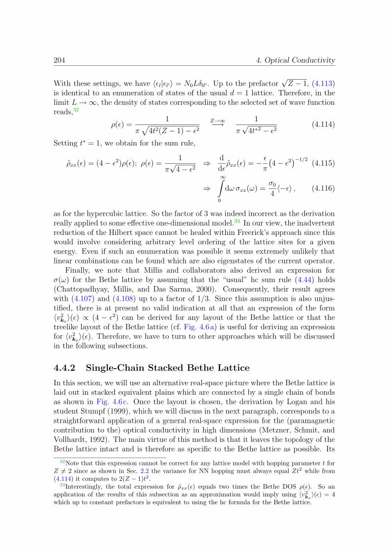
204 4. Optical Conductivity
With these settings, we have 〈εl|εl′〉 = N0Lδll′ . Up to the prefactor√Z − 1, (4.113)
is identical to an enumeration of states of the usual d = 1 lattice. Therefore, in thelimit L→∞, the density of states corresponding to the selected set of wave functionreads,32
ρ(ε) =1
π√
4t2(Z − 1)− ε2Z→∞−→ 1
π√
4t∗2 − ε2(4.114)
Setting t∗ = 1, we obtain for the sum rule,
ρxx(ε) = (4− ε2)ρ(ε); ρ(ε) =1
π√
4− ε2⇒ d
dερxx(ε) = − ε
π
(4− ε2
)−1/2(4.115)
⇒∞∫
0
dω σxx(ω) =σ0
4〈−ε〉 , (4.116)
as for the hypercubic lattice. So the factor of 3 was indeed incorrect as the derivationreally applied to some effective one-dimensional model.33 In our view, the inadvertentreduction of the Hilbert space cannot be healed within Freerick’s approach since thiswould involve considering arbitrary level ordering of the lattice sites for a givenenergy. Even if such an enumeration was possible it seems extremely unlikely thatlinear combinations can be found which are also eigenstates of the current operator.
Finally, we note that Millis and collaborators also derived an expression forσ(ω) for the Bethe lattice by assuming that the “usual” hc sum rule (4.44) holds(Chattopadhyay, Millis, and Das Sarma, 2000). Consequently, their result agreeswith (4.107) and (4.108) up to a factor of 1/3. Since this assumption is also unjus-tified, there is at present no valid indication at all that an expression of the form〈v2
kx〉(ε) ∝ (4 − ε2) can be derived for any layout of the Bethe lattice or that the
treelike layout of the Bethe lattice (cf. Fig. 4.6a) is useful for deriving an expressionfor 〈v2
kx〉(ε). Therefore, we have to turn to other approaches which will be discussed
in the following subsections.
4.4.2 Single-Chain Stacked Bethe Lattice
In this section, we will use an alternative real-space picture where the Bethe lattice islaid out in stacked equivalent plains which are connected by a single chain of bondsas shown in Fig. 4.6c. Once the layout is chosen, the derivation by Logan and hisstudent Stumpf (1999), which we will discuss in the next paragraph, corresponds to astraightforward application of a general real-space expression for the (paramagneticcontribution to the) optical conductivity in high dimensions (Metzner, Schmit, andVollhardt, 1992). The main virtue of this method is that it leaves the topology of theBethe lattice intact and is therefore as specific to the Bethe lattice as possible. Its
32Note that this expression cannot be correct for any lattice model with hopping parameter t forZ 6= 2 since as shown in Sec. 2.2 the variance for NN hopping must always equal Zt2 while from(4.114) it computes to 2(Z − 1)t2.
33Interestingly, the total expression for ρxx(ε) equals two times the Bethe DOS ρ(ε). So anapplication of the results of this subsection as an approximation would imply using 〈v2
kx〉(ε) = 4
which up to constant prefactors is equivalent to using the hc formula for the Bethe lattice.
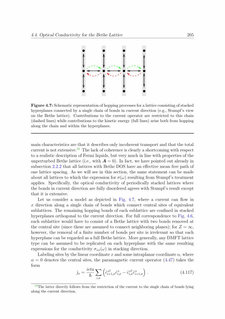
4.4. Optical Conductivity for the Bethe Lattice 205
Figure 4.7: Schematic representation of hopping processes for a lattice consisting of stackedhyperplanes connected by a single chain of bonds in current direction (e.g., Stumpf’s viewon the Bethe lattice). Contributions to the current operator are restricted to this chain(dashed lines) while contributions to the kinetic energy (full lines) arise both from hoppingalong the chain and within the hyperplanes.
main characteristics are that it describes only incoherent transport and that the totalcurrent is not extensive.34 The lack of coherence is clearly a shortcoming with respectto a realistic description of Fermi liquids, but very much in line with properties of theunperturbed Bethe lattice (i.e., with A = 0). In fact, we have pointed out already insubsection 2.2.2 that all lattices with Bethe DOS have an effective mean free path ofone lattice spacing. As we will see in this section, the same statement can be madeabout all lattices to which the expression for σ(ω) resulting from Stumpf’s treatmentapplies. Specifically, the optical conductivity of periodically stacked lattices wherethe bonds in current direction are fully disordered agrees with Stumpf’s result exceptthat it is extensive.
Let us consider a model as depicted in Fig. 4.7, where a current can flow inx direction along a single chain of bonds which connect central sites of equivalentsublattices. The remaining hopping bonds of each sublattice are confined in stackedhyperplanes orthogonal to the current direction. For full correspondence to Fig. 4.6,each sublattice would have to consist of a Bethe lattice with two bonds removed atthe central site (since these are assumed to connect neighboring planes); for Z =∞,however, the removal of a finite number of bonds per site is irrelevant so that eachhyperplane can be regarded as a full Bethe lattice. More generally, any DMFT latticetype can be assumed to be replicated on each hyperplane with the same resultingexpressions for the conductivity σxx(ω) in stacking direction.
Labeling sites by the linear coordinate x and some intraplanar coordinate α, whereα = 0 denotes the central sites, the paramagnetic current operator (4.47) takes theform
x =ieta
~
∑
i,σ
(
c 0†i+1,σ c
0
i,σ − c 0†i,σ c
0
i+1,σ
)
. (4.117)
34The latter directly follows from the restriction of the current to the single chain of bonds lyingalong the current direction.

206 4. Optical Conductivity
··
··
··
··
··
TT
TT
TT
TT
TT
TT
TT
TT
TT
TT
··
··
··
··
··
··
··
··
··
··
TT
TT
TT
TT
TT
TT
TT
TT
TT
TT
··
··
··
··
··
··
··
··
··
··
TT
TT
TT
TT
TT
TT
TT
TT
TT
TT
··
··
··
··
··
··
··
··
··
··
TT
TT
TT
TT
TT
TT
TT
TT
TT
TT
··
··
··
··
··
a) b)
c) d)
Figure 4.8: Diagrammatic representation of terms of the form (4.119) entering the com-putation of the optical conductivity: a) Leading contribution scaling as O(1/Z). b) andc) subleading contributions being O(1/Z2). d) Contributions which include loops do notexist for the Bethe lattice (but are among the leading diagrams for regular lattices).
Here, the upper index 0 of operators stands for α = 0, the central site within asublattice. Consequently, the paramagnetic contribution to the optical conductivity
σxx(ω) = − e2a2t2
i~2(ω + i0+)N
∑
i,j,σ
〈〈c 0†i+1,σ c
0
i,σ − c 0†i,σ c
0
i+1,σ, c0†j+1,σ c
0
j,σ − c 0†j,σ c
0
j+1,σ 〉〉(ω + i0+)
(4.118)contains terms of the form (with suppressed ω-dependence)
Γijkm := 〈〈c 0†iσ c
0
kσ, c0†mσ c
0
jσ 〉〉δi,k±1δm,j±1 . (4.119)
In a diagrammatic evaluation of the corresponding real-time correlation function (cf.Sec. D.2), the exponentials carrying the time dependence in the Heisenberg pictureintroduce additional paths between pairs of sites; the resulting full diagram onlycontributes to the implicit trace when it represents a closed path. A selection of suchdiagrams is shown in Fig. 4.8 where the current paths35 (dashed lines) are closed bytime-dependent propagators (solid lines). In the DMFT formalism, each path of taxi-cab length l carries a factor of Z−l/2 so that the diagrams in Fig. 4.8a, Fig. 4.8b, andFig. 4.8c, have prefactors of 1/Z, 1/Z2, and 1/Z2, respectively. Due to the absenceof loops, the additional powers of 1/Z introduced by nonlocal propagators cannotbe compensated by factors of Z arising from a sum over equivalent diagrams. Thus,up to a shift along the current direction, diagram Fig. 4.8a is the only (leading)contribution for Z → ∞. For comparison, a diagram typical of regular lattices isshown in Fig. 4.8d; such diagrams usually contribute in leading order Z/Z2, but donot exist on the Bethe lattice. The two time-dependent propagators closing the pathdo not interfere for Z → ∞ on any lattice (see subsection 4.4.4) which implies that
35In momentum representation, these “current vertices” contract to a pair of dots.
4.4. Optical Conductivity for the Bethe Lattice 207
the expectation values decouple and lead to a pair of single-particle Green functions,i.e., to the usual bubble sum. In the specific case under consideration, i.e., withoutloops, both Green functions become local, so that the conductivity reads
σxx(ω) =πe2a2t2
~2
LxL
∑
σ
∞∫
−∞
dω′AAσ(ω′)ABσ(ω
′ + ω)nf(ω
′)− nf(ω′ + ω)
ω. (4.120)
Here, A(ω) denotes the full local spectral function, Lx the linear extent in currentdirection, and L the number of sites for some finite part of the system. As indicatedby the sublattice indices A,B and spin index σ, the result is valid also in phases withbroken symmetry, i.e., in an antiferromagnetic phase. Note that (4.120) is not directlydependent on the type of the underlying sublattice (confined in each hyperplane), noteven via a noninteracting DOS.36
The most striking feature of the present derivation and its result (4.120) is thatthe dc conductivity always remains finite (or vanishes) in the paramagnetic phase,even in the noninteracting limit. This follows from the fact that in the paramagneticphase, the local spectral function is bounded by the maximum of the noninteract-ing DOS. For a symmetric DOS which is peaked at zero frequency, the integral in(4.120) is therefore bounded by ρ2(0).37 Consequently, there is no qualitative differ-ence between the conductivities for noninteracting and interacting systems: only theenergy eigenvalues of each pair of states determines its contribution to σxx(ω); theassociated momenta are unimportant. This behavior is in striking contrast to theBravais lattice case discussed in subsection 4.1.4 where the dc conductivity divergesin the noninteracting limit. In this sense, (4.120) describes incoherent transport. Aswe will show in subsection 4.5.1, the expression is generally valid within the DMFTfor k⊥-nonconserving hopping between planes.
Commutators and Loops
As discussed in subsection 4.1.4, the presence of optical absorption at finite frequen-cies in the noninteracting limit implies that the paramagnetic current operator andthe kinetic energy do not commute. In the following, we will demonstrate that indeed[H0, ] 6= 0 for the single-chain layout discussed in this subsection. For this purpose,we focus first on a single contribution to the current operator and study separatelyand in turn its commutator with kinetic energy contributions (anti)parallel or per-pendicular to its direction. We will see that the former contributions vanish quitegenerically (in absence of disorder) in summations along the current chains. In con-trast, the latter contributions can only cancel in the presence of certain loops oflength four which do not exist on the Bethe lattice.
For a single hopping term contributing to the current operator, the commutator
36In subsection 4.5.1, we will present a unified treatment of incoherent and coherent transportwhere k-sums and noninteracting DOSs reappear for the case of regular sublattices.
37In contrast, momentum-dependent spectral functions diverge in the noninteracting limit.
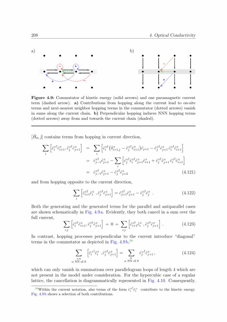
208 4. Optical Conductivity
+
+−
−
−
+
a) b)
Figure 4.9: Commutator of kinetic energy (solid arrows) and one paramagnetic currentterm (dashed arrow). a) Contributions from hopping along the current lead to on-siteterms and next-nearest neighbor hopping terms in the commutator (dotted arrows) vanishin sums along the current chain. b) Perpendicular hopping induces NNN hopping terms(dotted arrows) away from and towards the current chain (shaded).
[H0, ] contains terms from hopping in current direction,
∑
i
[
c 0†i c
0
i+1, c0†j c
0
j+1
]
=∑
i
[
c 0†i
(δ 0
i+1,j − c 0†j c
0
i+1
)cj+1 − c 0†
j c0
j+1 c0†i c
0
i+1
]
= c 0†j−1c
0
j+1 −∑
i
[
c 0†j c
0†i c
0
j+1c0
i+1 + c 0†j c
0
j+1 c0†i c
0
i+1
]
= c 0†j−1c
0
j+1 − c 0†j c
0
j+2 (4.121)
and from hopping opposite to the current direction,
∑
i
[
c 0†i+1c
0
i , c0†j c
0
j+1
]
= c 0†j+1c
0
j+1 − c 0†j c
0
j . (4.122)
Both the generating and the generated terms for the parallel and antiparallel casesare shown schematically in Fig. 4.9a. Evidently, they both cancel in a sum over thefull current,
∑
i,j
[
c 0†i c
0
i+1, c0†j c
0
j+1
]
= 0 =∑
i,j
[
c 0†i+1c
0
i , c0†j c
0
j+1
]
. (4.123)
In contrast, hopping processes perpendicular to the current introduce “diagonal”terms in the commutator as depicted in Fig. 4.9b,38
∑
i,αα NN of 0
[
cα†i c 0
i , c0†j c
0
j+1
]
=∑
αα NN of 0
cα†j c 0
j+1 , (4.124)
which can only vanish in summations over parallelogram loops of length 4 which arenot present in the model under consideration. For the hypercubic case of a regularlattice, the cancellation is diagrammatically represented in Fig. 4.10. Consequently,
38Within the current notation, also terms of the form c 0†i c α
i contribute to the kinetic energy.Fig. 4.9b shows a selection of both contributions.
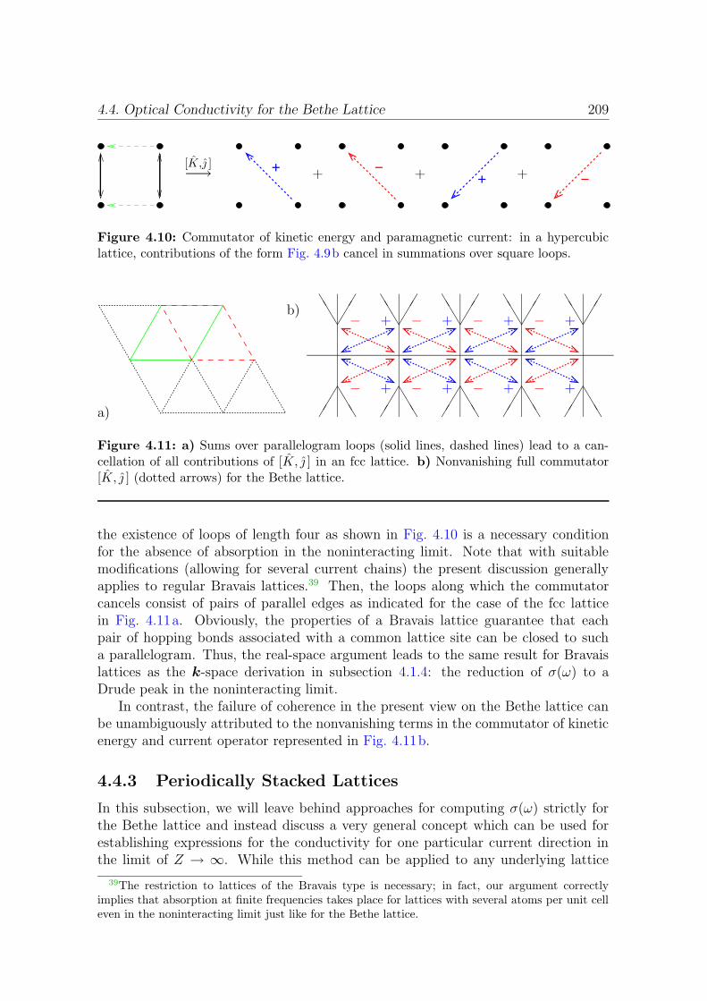
4.4. Optical Conductivity for the Bethe Lattice 209
[K, ]−→ ++
−−+ + +
Figure 4.10: Commutator of kinetic energy and paramagnetic current: in a hypercubiclattice, contributions of the form Fig. 4.9b cancel in summations over square loops.
− − − −
− − − −
+ + + +
+ + + +
···
···
···
···
···
TTT
TTT
TTT
TTT
TTT
TTT
TTT
TTT
TTT
TTT
···
···
···
···
···
a)
b)
Figure 4.11: a) Sums over parallelogram loops (solid lines, dashed lines) lead to a can-cellation of all contributions of [K, ] in an fcc lattice. b) Nonvanishing full commutator[K, ] (dotted arrows) for the Bethe lattice.
the existence of loops of length four as shown in Fig. 4.10 is a necessary conditionfor the absence of absorption in the noninteracting limit. Note that with suitablemodifications (allowing for several current chains) the present discussion generallyapplies to regular Bravais lattices.39 Then, the loops along which the commutatorcancels consist of pairs of parallel edges as indicated for the case of the fcc latticein Fig. 4.11a. Obviously, the properties of a Bravais lattice guarantee that eachpair of hopping bonds associated with a common lattice site can be closed to sucha parallelogram. Thus, the real-space argument leads to the same result for Bravaislattices as the k-space derivation in subsection 4.1.4: the reduction of σ(ω) to aDrude peak in the noninteracting limit.
In contrast, the failure of coherence in the present view on the Bethe lattice canbe unambiguously attributed to the nonvanishing terms in the commutator of kineticenergy and current operator represented in Fig. 4.11b.
4.4.3 Periodically Stacked Lattices
In this subsection, we will leave behind approaches for computing σ(ω) strictly forthe Bethe lattice and instead discuss a very general concept which can be used forestablishing expressions for the conductivity for one particular current direction inthe limit of Z → ∞. While this method can be applied to any underlying lattice
39The restriction to lattices of the Bravais type is necessary; in fact, our argument correctlyimplies that absorption at finite frequencies takes place for lattices with several atoms per unit celleven in the noninteracting limit just like for the Bethe lattice.
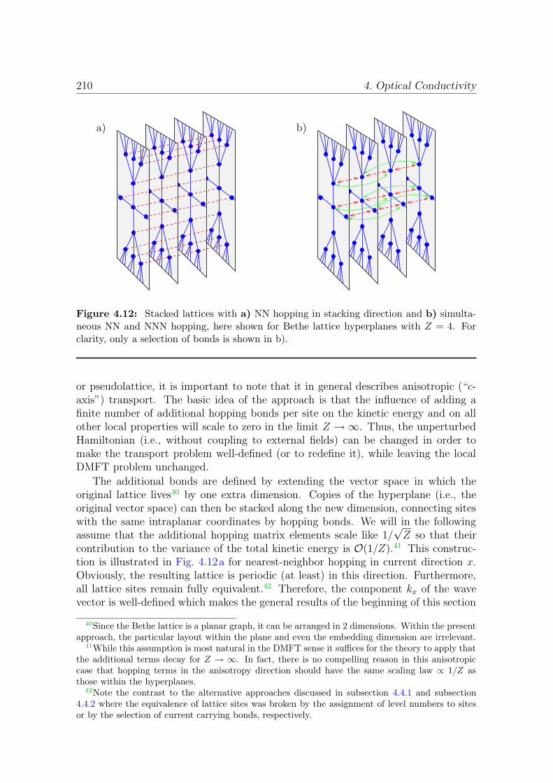
210 4. Optical Conductivity
a) b)
Figure 4.12: Stacked lattices with a) NN hopping in stacking direction and b) simulta-neous NN and NNN hopping, here shown for Bethe lattice hyperplanes with Z = 4. Forclarity, only a selection of bonds is shown in b).
or pseudolattice, it is important to note that it in general describes anisotropic (“c-axis”) transport. The basic idea of the approach is that the influence of adding afinite number of additional hopping bonds per site on the kinetic energy and on allother local properties will scale to zero in the limit Z →∞. Thus, the unperturbedHamiltonian (i.e., without coupling to external fields) can be changed in order tomake the transport problem well-defined (or to redefine it), while leaving the localDMFT problem unchanged.
The additional bonds are defined by extending the vector space in which theoriginal lattice lives40 by one extra dimension. Copies of the hyperplane (i.e., theoriginal vector space) can then be stacked along the new dimension, connecting siteswith the same intraplanar coordinates by hopping bonds. We will in the followingassume that the additional hopping matrix elements scale like 1/
√Z so that their
contribution to the variance of the total kinetic energy is O(1/Z).41 This construc-tion is illustrated in Fig. 4.12a for nearest-neighbor hopping in current direction x.Obviously, the resulting lattice is periodic (at least) in this direction. Furthermore,all lattice sites remain fully equivalent.42 Therefore, the component kx of the wavevector is well-defined which makes the general results of the beginning of this section
40Since the Bethe lattice is a planar graph, it can be arranged in 2 dimensions. Within the presentapproach, the particular layout within the plane and even the embedding dimension are irrelevant.
41While this assumption is most natural in the DMFT sense it suffices for the theory to apply thatthe additional terms decay for Z → ∞. In fact, there is no compelling reason in this anisotropiccase that hopping terms in the anisotropy direction should have the same scaling law ∝ 1/Z asthose within the hyperplanes.
42Note the contrast to the alternative approaches discussed in subsection 4.4.1 and subsection4.4.2 where the equivalence of lattice sites was broken by the assignment of level numbers to sitesor by the selection of current carrying bonds, respectively.

4.4. Optical Conductivity for the Bethe Lattice 211
applicable. For NN hopping in current direction, the conductivity is thus given by
Re σxx(ω) =2πe2a2t2
~2
N
V
∞∫
−∞
dερ(ε)
∞∫
−∞
dω′Aε(ω′)Aε(ω
′ + ω)nf(ω
′)− nf(ω + ω′)
ω,
(4.125)which agrees with (4.73) for a uniform hopping amplitude t = t∗/
√d. For the par-
ticular case of the stacked Bethe lattice, this fact was observed and used by Uhrigand Vlaming (1993). Longer-range hopping in stacking direction as illustrated inFig. 4.12b only leads to a modified constant prefactor. For this general case, anexpression for σxx(ω) is found from (4.65) in conjunction with (4.75).
As verified by Uhrig and Vlaming (1993) within their locator formalism, the result-ing sum rule for NN hopping in current direction is indeed of the form characteristicfor the hypercubic lattice [with σ0 = 2πe2N/(V ~
2) as defined in (4.67)],
∞∫
0
dω σxx(ω) = −σ0t2a2
4〈Tx〉 . (4.126)
This observation is, however, not very useful in the DMFT context since the applica-bility of (4.125) depended on the fact that 〈Tx〉 is negligible with respect to the fullkinetic energy. Thus, (4.126) alone gives no relation between the frequency sum andany expectation value surviving the DMFT limit. Using instead the general DMFTf -sum rule (4.87), we obtain for the general stacked case,
∞∫
0
dω σxx(ω) =σ0
4〈
ddερ(ε)
ρ(ε)〉
2π/ax∫
0
dkxv2kx, (4.127)
where the integral equals t2a2 for NN hopping in current direction. Thus, we have notonly identified a form of the f -sum rule which is generally applicable for anisotropiclattices in high dimensions, but also found an expression for the expectation valueof the kinetic energy in the stacking direction. For the particular case of the stackedBethe lattice with NN hopping, the sum rule reads [cf. (4.97)]
∞∫
0
dω σxx(ω) =t2a2σ0
4〈 −ε4− ε2 〉 . (4.128)
4.4.4 Offdiagonal Disorder
In the DMFT limit, diagrammatic expressions for directional transport are alwaysdominated by diagrams with minimal extent in current direction. Specifically, forlattices where all lattice sites are arranged in planes perpendicular to the currentand where the interplane contribution to the kinetic energy has zero weight for Z →∞, the surviving diagrams are confined to two neighboring planes with only twoconnections, the current vertices, between the planes as illustrated in Fig. 4.13: here
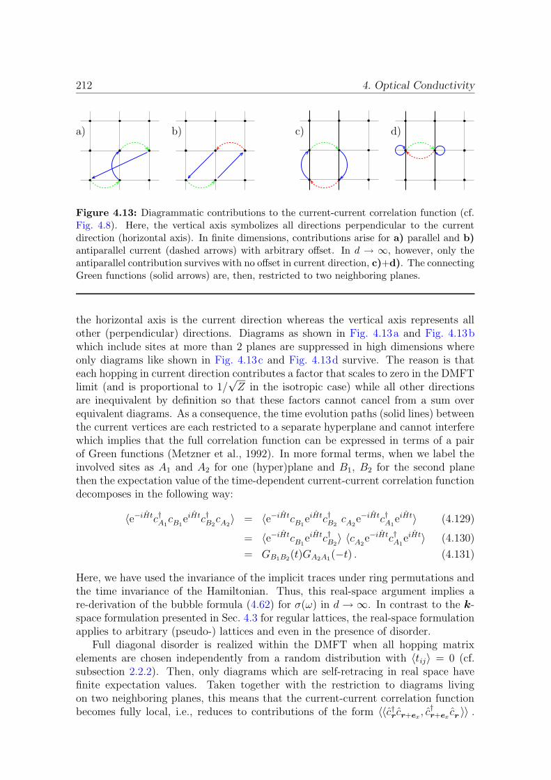
212 4. Optical Conductivity
a) b) c) d)
Figure 4.13: Diagrammatic contributions to the current-current correlation function (cf.Fig. 4.8). Here, the vertical axis symbolizes all directions perpendicular to the currentdirection (horizontal axis). In finite dimensions, contributions arise for a) parallel and b)antiparallel current (dashed arrows) with arbitrary offset. In d → ∞, however, only theantiparallel contribution survives with no offset in current direction, c)+d). The connectingGreen functions (solid arrows) are, then, restricted to two neighboring planes.
the horizontal axis is the current direction whereas the vertical axis represents allother (perpendicular) directions. Diagrams as shown in Fig. 4.13a and Fig. 4.13bwhich include sites at more than 2 planes are suppressed in high dimensions whereonly diagrams like shown in Fig. 4.13c and Fig. 4.13d survive. The reason is thateach hopping in current direction contributes a factor that scales to zero in the DMFTlimit (and is proportional to 1/
√Z in the isotropic case) while all other directions
are inequivalent by definition so that these factors cannot cancel from a sum overequivalent diagrams. As a consequence, the time evolution paths (solid lines) betweenthe current vertices are each restricted to a separate hyperplane and cannot interferewhich implies that the full correlation function can be expressed in terms of a pairof Green functions (Metzner et al., 1992). In more formal terms, when we label theinvolved sites as A1 and A2 for one (hyper)plane and B1, B2 for the second planethen the expectation value of the time-dependent current-current correlation functiondecomposes in the following way:
〈e−iHtc†A1cB1
eiHtc†B2cA2〉 = 〈e−iHtcB1
eiHtc†B2cA2
e−iHtc†A1eiHt〉 (4.129)
= 〈e−iHtcB1eiHtc†B2
〉 〈cA2e−iHtc†A1
eiHt〉 (4.130)
= GB1B2(t)GA2A1
(−t) . (4.131)
Here, we have used the invariance of the implicit traces under ring permutations andthe time invariance of the Hamiltonian. Thus, this real-space argument implies are-derivation of the bubble formula (4.62) for σ(ω) in d → ∞. In contrast to the k-space formulation presented in Sec. 4.3 for regular lattices, the real-space formulationapplies to arbitrary (pseudo-) lattices and even in the presence of disorder.
Full diagonal disorder is realized within the DMFT when all hopping matrixelements are chosen independently from a random distribution with 〈tij〉 = 0 (cf.subsection 2.2.2). Then, only diagrams which are self-retracing in real space havefinite expectation values. Taken together with the restriction to diagrams livingon two neighboring planes, this means that the current-current correlation functionbecomes fully local, i.e., reduces to contributions of the form 〈〈c†r cr+ex
, c†r+excr 〉〉 .
4.4. Optical Conductivity for the Bethe Lattice 213
Consequently, the optical conductivity can be expressed in terms of local spectralfunctions (Dobrosavljevic and Kotliar, 1993),
σxx(ω) =πe2a2t2
~2
N
V
∑
σ
∞∫
−∞
dω′AAσ(ω′)ABσ(ω
′ + ω)nf(ω
′)− nf(ω′ + ω)
ω, (4.132)
where t2 = 〈t2r,r+ex〉. Note that this expression essentially agrees with (4.120), but
does not contain the factor Lx/L which scales to zero in the thermodynamic limit.We also observe that (4.132) is valid as long as the hopping terms in current directionare fully disordered in the sense defined above regardless if the bonds perpendicularto the current (i.e., within the hyperplanes) are ordered or disordered. This resultcan, therefore, be applied in connection with any underlying lattice and is, then,characteristic of the stacked disordered anisotropic model.
4.4.5 General Dispersion Method
In the preceding subsections, we have seen that all previous approaches of definingand computing an optical conductivity compatible with DMFT calculations for asemi-elliptic DOS had an inherently anisotropic character. Using the general formal-ism developed in Sec. 2.3 and applied to the Bethe DOS in Sec. 2.4, we can herefor the first time consider the isotropic case. We remind the reader that in the gen-eral dispersion formalism hopping matrix elements only depend on taxi-cab distanceD which, for d → ∞, leads to the dispersion εk =
∑∞D=1 HeD(εhc
k ) t∗D/√D!, where
HeD(x) is the Hermite polynomial of order D and εhck is the dispersion of the hyper-
cubic lattice with NN hopping [cf. (2.52)]. Due to the completeness of the Hermitepolynomials, an arbitrary transformation function f with εk = f(εhc
k ) can be real-ized by an appropriate choice of scaled hopping matrix elements t∗D. In particular,any bounded function f leads to corresponding band edges in the resulting DOS.Using (2.61), a suitable (monotonous) transformation function f may be determinedfor an arbitrary “target” DOS which then allows for the computation of transportproperties, e.g., via (2.63). Furthermore, the hopping matrix elements defining thecorresponding microscopic model can be computed according to (2.55).
For the “redefined Bethe lattice”, a regular isotropic hc lattice with extendedhopping along the diagonals and a semi-elliptic DOS, we have from (2.70),
ρ(ε) =1
2√
1− ε2/4exp
−2
(
erf−1(ε√
1− ε2/4 + 2 sin−1(ε/2)
π
)
)2
(4.133)
which defines σxx(ω) in conjunction with the general expression (4.65) and is shown inFig. 4.14. Also shown in the figure is the function ρ′(ε)/ρ(ε) which determines the sumrule (4.95). It is a straightforward but lengthy exercise to derive the explicit analyticexpression from the chain rule. Let us, instead, only point out that it approaches−πε/2 at ε ≈ 0, but clearly deviates from this asymptotic form near the band edges.Thus, the f -sum cannot be proportional to the kinetic energy in any limit. The
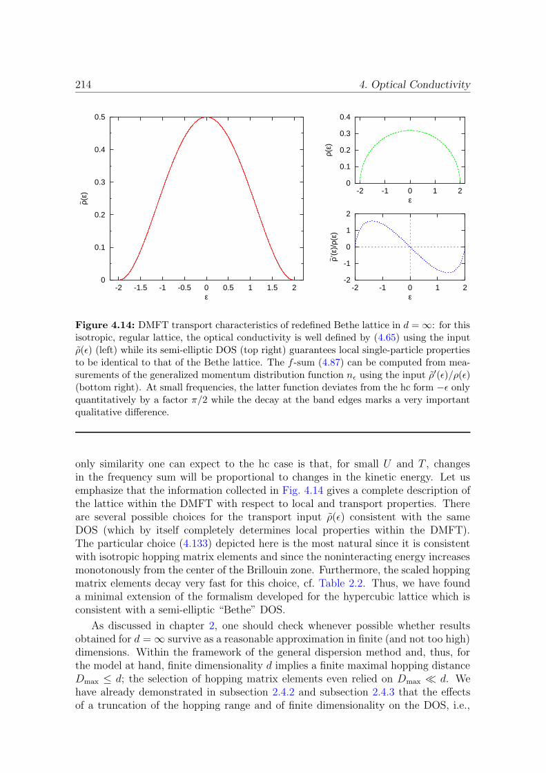
214 4. Optical Conductivity
0
0.1
0.2
0.3
0.4
0.5
-2 -1.5 -1 -0.5 0 0.5 1 1.5 2
~ ρ(ε)
ε
0
0.1
0.2
0.3
0.4
-2 -1 0 1 2
ρ(ε)
ε
-2
-1
0
1
2
-2 -1 0 1 2
~ ρ’(ε
)/ρ(
ε)
ε
Figure 4.14: DMFT transport characteristics of redefined Bethe lattice in d =∞: for thisisotropic, regular lattice, the optical conductivity is well defined by (4.65) using the inputρ(ε) (left) while its semi-elliptic DOS (top right) guarantees local single-particle propertiesto be identical to that of the Bethe lattice. The f -sum (4.87) can be computed from mea-surements of the generalized momentum distribution function nε using the input ρ′(ε)/ρ(ε)(bottom right). At small frequencies, the latter function deviates from the hc form −ε onlyquantitatively by a factor π/2 while the decay at the band edges marks a very importantqualitative difference.
only similarity one can expect to the hc case is that, for small U and T , changesin the frequency sum will be proportional to changes in the kinetic energy. Let usemphasize that the information collected in Fig. 4.14 gives a complete description ofthe lattice within the DMFT with respect to local and transport properties. Thereare several possible choices for the transport input ρ(ε) consistent with the sameDOS (which by itself completely determines local properties within the DMFT).The particular choice (4.133) depicted here is the most natural since it is consistentwith isotropic hopping matrix elements and since the noninteracting energy increasesmonotonously from the center of the Brillouin zone. Furthermore, the scaled hoppingmatrix elements decay very fast for this choice, cf. Table 2.2. Thus, we have founda minimal extension of the formalism developed for the hypercubic lattice which isconsistent with a semi-elliptic “Bethe” DOS.
As discussed in chapter 2, one should check whenever possible whether resultsobtained for d =∞ survive as a reasonable approximation in finite (and not too high)dimensions. Within the framework of the general dispersion method and, thus, forthe model at hand, finite dimensionality d implies a finite maximal hopping distanceDmax ≤ d; the selection of hopping matrix elements even relied on Dmax ¿ d. Wehave already demonstrated in subsection 2.4.2 and subsection 2.4.3 that the effectsof a truncation of the hopping range and of finite dimensionality on the DOS, i.e.,
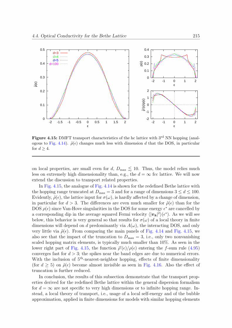
4.4. Optical Conductivity for the Bethe Lattice 215
0
0.1
0.2
0.3
0.4
0.5
-2 -1.5 -1 -0.5 0 0.5 1 1.5 2
~ ρ(ε)
ε
d=3d=4d=5
d=100
0
0.1
0.2
0.3
0.4
-2 -1 0 1 2
ρ(ε)
ε
-2
-1
0
1
2
-2 -1 0 1 2
~ ρ’(ε
)/ρ(
ε)
ε
Figure 4.15: DMFT transport characteristics of the hc lattice with 3rd NN hopping (anal-ogous to Fig. 4.14). ρ(ε) changes much less with dimension d that the DOS, in particularfor d ≥ 4.
on local properties, are small even for d, Dmax . 10. Thus, the model relies muchless on extremely high dimensionality than, e.g., the d =∞ fcc lattice. We will nowextend the discussion to transport related properties.
In Fig. 4.15, the analogue of Fig. 4.14 is shown for the redefined Bethe lattice withthe hopping range truncated at Dmax = 3 and for a range of dimensions 3 ≤ d ≤ 100.Evidently, ρ(ε), the lattice input for σ(ω), is hardly affected by a change of dimension,in particular for d > 3. The differences are even much smaller for ρ(ε) than for theDOS ρ(ε) since Van-Hove singularities in the DOS for some energy ε∗ are cancelled bya corresponding dip in the average squared Fermi velocity 〈|vk|2〉(ε∗). As we will seebelow, this behavior is very general so that results for σ(ω) of a local theory in finitedimensions will depend on d predominantly via A(ω), the interacting DOS, and onlyvery little via ρ(ε). From comparing the main panels of Fig. 4.14 and Fig. 4.15, wealso see that the impact of the truncation to Dmax = 3, i.e., only two nonvanishingscaled hopping matrix elements, is typically much smaller than 10%. As seen in thelower right part of Fig. 4.15, the function ρ′(ε)/ρ(ε) entering the f -sum rule (4.95)converges fast for d > 3; the spikes near the band edges are due to numerical errors.With the inclusion of 5th-nearest-neighbor hopping, effects of finite dimensionality(for d ≥ 5) on ρ(ε) become almost invisible as seen in Fig. 4.16. Also the effect oftruncation is further reduced.
In conclusion, the results of this subsection demonstrate that the transport prop-erties derived for the redefined Bethe lattice within the general dispersion formalismfor d = ∞ are not specific to very high dimensions or to infinite hopping range. In-stead, a local theory of transport, i.e., usage of a local self-energy and of the bubbleapproximation, applied in finite dimensions for models with similar hopping elements

216 4. Optical Conductivity
0
0.1
0.2
0.3
0.4
0.5
-2 -1.5 -1 -0.5 0 0.5 1 1.5 2
~ ρ(ε)
ε
d=5d=6
d=100
0
0.1
0.2
0.3
0.4
-2 -1 0 1 2
ρ(ε)
ε
-2
-1
0
1
2
-2 -1 0 1 2
~ ρ’(ε
)/ρ(
ε)
ε
Figure 4.16: DMFT transport characteristics of hc lattice with 5th NN hopping (analogousto Fig. 4.14). ρ(ε) is practically independent of dimension.
leads to similar expressions for σ(ω) and would, thus, also lead to similar results. Inthis sense, the final numerical results which we will present in Sec. 4.6 are not spe-cific to the limit d = ∞, but apply at least qualitatively also for a local theory ofconductivity in finite d, as long as the noninteracting DOS is symmetric and roughlysemi-elliptic.
4.5 Generalizations
In the previous section, we have focused on the question of how to define and computeσ(ω) in a way consistent with DMFT calculations for a semi-elliptic noninteractingDOS and within the paramagnetic phase. Before showing numerical results basedon these studies in the next subsection, we use this section to present generalizingconcepts. In subsection 4.5.1, we discuss various cases of stacked lattices which lead tovarious degrees of coherence in the transport along the stacking direction. Propertiesentering a local theory of σ(ω) in finite dimensions are collected for various latticetypes in subsection 4.5.2. Finally, the effect of frustration on transport is studiedanalytically using the t − t′ lattice, i.e., a hc lattice with NN and NNN hopping insubsection 4.5.3.
4.5.1 Coherent versus Incoherent Transport in High Dimen-sions
As discussed in subsection 4.4.4, diagrammatic contributions to the optical conductiv-ity along a symmetry direction generically only involve two neighboring hyperplanes.

4.5. Generalizations 217
Therefore, the Green functions appearing in the bubble formula for σ(ω) are local inthe current direction. Let us for the moment specialize in the general stacked casewhere the hyperplanes are connected by nearest-neighbor bonds in current directionwhich is assumed to be perpendicular to the hyperplanes. If we consider the homo-geneous case and denote the real space Green function connecting site r1 and r2 asGr2−r1
(ω), the resulting expression contributing to the conductivity is of the form
∑
r⊥
G(0,r⊥)(ω) G(0,−r⊥)(ω′) . (4.134)
The important point is that the Green functions are local in current direction; r⊥is the perpendicular component of r. If the hyperplanes are regular lattices, thistranslates in Fourier space into a contribution
∑
k
∑
k′
Gk(ω)Gk′(ω′) δ(k⊥ − k′⊥) . (4.135)
This simple form applies to the hypercubic lattice and all “full” stacked lattices,where each lattice site is connected to neighboring sites by bonds in current direction.Compared with the finite-dimensional case where the bubble summation would haveto include diagrams as shown in Fig. 4.13c and which would give rise to the full δ-function δ(k−k′), the restriction of the δ-function to perpendicular directions mightalready be viewed as a reduction of coherence. Obviously the fully incoherent case isrealized when there is only a single chain of links in current direction as discussed insubsection 4.4.2 or if the hopping in current direction is fully disordered as discussedin subsection 4.4.4: in both cases, the δ-function is replaced by unity.
The main point of this subsection is that the degree of coherence in k⊥ may betuned for an anisotropic model by attaching bonds in current direction only to asublattice of sites within each hyperplane (with the extreme cases where sublatticeand full lattice within the hyperplane are identical or when only a single site per planeis connected). For example, when every second site (i.e., any site with coordinates rfor which (−1)||r⊥|| = 1) is connected, the transport is coherent up to the AF wavevector which leads to a contribution43
∑
k
∑
k′
Gk(ω)Gk′(ω′)1
2
(δ(k⊥ − k′
⊥) + δ(k⊥ − k′⊥ −Q⊥)
). (4.136)
Finally, for a hc lattice (with arbitrary hopping range in the perpendicular direction)where every nth
α site in direction α is part of the “current sublattice”, the k summationreads
∑
k
∑
k′
Gk(ω)Gk′(ω′)d∏
α=2
(
1
nα
nα−1∑
l=0
δ(kα − k′α −l
nα
2π
aα)
)
. (4.137)
Here, aα is the lattice spacing in direction α. The completely incoherent case isrecovered for nα →∞ when all δ-functions approach unity.

218 4. Optical Conductivity
a) b) c) d)
Figure 4.17: a) For stacked lattices with only one current chain (here in horizontal di-rection), the current-current correlation function reduces to its (antiparallel) on-bond part;the Green functions become local. b) For stacked lattices with interplane connections onlyfor every second site, the connecting Green functions (solid arrows) are diagonal in sublat-tice index α ∈ A,B. c)+d) Generalized stacked lattices with additional hopping alongdiagonals (see text).
A complementary view is taken in Fig. 4.17. While the completely incoherentcase with a single link in current direction leads to diagrams involving only localGreen functions as shown in Fig. 4.17a, the case where current bonds touch everysecond site implies diagrams where all Green functions are local with respect to thesublattice index as shown in Fig. 4.17b. Thus, the lack of coherence with respect toQ as demonstrated in (4.136) translates into a locality of the Green functions withrespect to the sublattice index.
In the more general case that current may also flow along diagonals, the two Greenfunctions do no longer only connect equivalent pairs of sites so that nontrivial factorsappear in the momentum summation. For example, NNN bonds imply diagrams asshown in Fig. 4.17c which lead to contributions of the form
2t‖ t′‖∑
k
∑
k′
Gk(ω)Gk′(ω′)(∑
α
cos(kα))
δ(k⊥ − k′⊥) (4.138)
and diagrams as shown in Fig. 4.17d with contributions44
4t′2‖∑
k
∑
k′
Gk(ω)Gk′(ω′)(∑
α
cos(kα))(∑
α′
cos(kα′))
δ(k⊥ − k′⊥) . (4.139)
Here, t‖ and t′‖ denote hopping matrix elements which contribute to the current
(and may differ from matrix elements for transport within the planes). Using theseand analogous considerations it is easily possible to derive expressions for σ(ω) forarbitrary stacked versions of arbitrary underlying regular lattices. One can evencarry out the momentum sums and, thus, arrive at expressions ρxx(ε) for any suchcombination. As one example, we remark that pure fcc-like hopping between planes as
43Note that this form immediately generalizes to the case of stacked AF planes (both with FMor AF order in current direction).
44It is easy to check that the special case α = α′ is properly accounted for in this equation. Indeedthe terms 2 cos(2kα) (corresponding to the actual diagram shown in Fig. 4.17d) and 2 (correspondingto parallel current vertices) sum up to 4 cos2(kα).

4.5. Generalizations 219
0
0.1
0.2
0.3
0.4
0.5
-3 -2 -1 0 1 2 3
~ ρ(ε)
ε
d=1d=2d=3d=4d=5
0
0.2
0.4
0.6
0.8
1
-3 -2 -1 0 1 2 3
ρ(ε)
ε
-3-2-10123
-3 -2 -1 0 1 2 3
~ ρ’(ε
)/ρ(
ε)
ε
Figure 4.18: DMFT transport characteristics of the hypercubic (hc) lattice with NNhopping (cf. Fig. 4.14). The approach of the limiting Gaussian form (for d → ∞) is muchfaster for ρ(ε) than for the DOS ρ(ε). The exact relation ρ′(ε)/ρ(ε) = −ε implies theproportionality of the f -sum to the kinetic energy.
described by (4.139) leads to v2k,x = 2dt′‖
2εhck2. If the hyperplanes are, e.g., hypercubic,
we get 〈v2k,x〉(ε) = 2dt′‖
2ε2. In contrast, if the hyperplanes are also of the fcc-type
with t′⊥ = t′‖ = t′∗√2d(d−1)
, the resulting expression is 〈v2k,x〉(ε) = 2 t
′∗2
d(1 +
√2
t′∗ε). In
the latter case we find that the squared Fermi velocity vanishes at the band edge asalways for isotropic systems.
4.5.2 Optical Conductivity in Finite Dimensions
In this subsection we continue the discussion of transport related lattice properties infinite dimensions for a series of commonly treated lattice types. With the exceptionof the dimension-independent analytic forms for ρ′(ε)/ρ(ε) available for the hc andfcc cases, all curves have been obtained by Monte Carlo sampling of the appropriatek-space expressions. Apart from possible uses of this data as input for computationsof σ(ω) in a local theory in finite dimensions, the study is also useful as supportfor the results of the general-dispersion method which may be used as a black-boxalgorithm for generating ρ(ε) from the noninteracting DOS ρ(ε) alone.
Fig. 4.18 shows that ρ(ε) converges much faster to its Gaussian d =∞ form thanthe DOS on the hc lattice. This is possible since van-Hove singularities appearing inthe DOS are cancelled by corresponding dips in the squared Fermi velocity. As visu-alized in Fig. 4.19a, the Fermi velocity becomes more and more effectively constantand approaches unity for d → ∞. In Fig. 4.19b corresponding curves are shown forthe fcc lattice which approach a tilted straight line vanishing at the band edge for
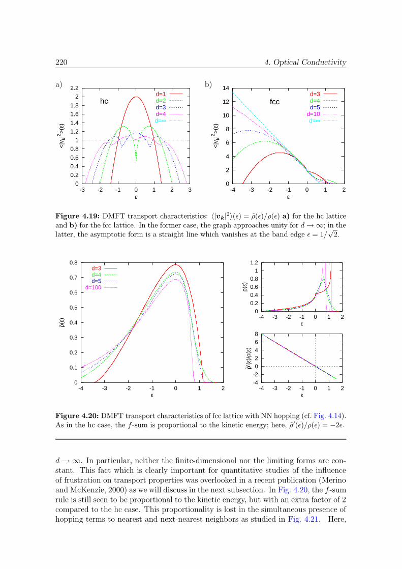
220 4. Optical Conductivity
a) b)
0
0.2
0.4
0.6
0.8
1
1.2
1.4
1.6
1.8
2
2.2
-3 -2 -1 0 1 2 3
<|v
k|2 >
(ε)
ε
hcd=1d=2d=3d=4d=∞
0
2
4
6
8
10
12
14
-4 -3 -2 -1 0 1 2
<|v
k|2 >
(ε)
ε
fccd=3d=4d=5
d=10d=∞
Figure 4.19: DMFT transport characteristics: 〈|vk|2〉(ε) = ρ(ε)/ρ(ε) a) for the hc latticeand b) for the fcc lattice. In the former case, the graph approaches unity for d→∞; in thelatter, the asymptotic form is a straight line which vanishes at the band edge ε = 1/
√2.
0
0.1
0.2
0.3
0.4
0.5
0.6
0.7
0.8
-4 -3 -2 -1 0 1 2
~ ρ(ε)
ε
d=3d=4d=5
d=100
00.20.40.60.8
11.2
-4 -3 -2 -1 0 1 2
ρ(ε)
ε
-4-202468
-4 -3 -2 -1 0 1 2
~ ρ’(ε
)/ρ(
ε)
ε
Figure 4.20: DMFT transport characteristics of fcc lattice with NN hopping (cf. Fig. 4.14).As in the hc case, the f -sum is proportional to the kinetic energy; here, ρ′(ε)/ρ(ε) = −2ε.
d→∞. In particular, neither the finite-dimensional nor the limiting forms are con-stant. This fact which is clearly important for quantitative studies of the influenceof frustration on transport properties was overlooked in a recent publication (Merinoand McKenzie, 2000) as we will discuss in the next subsection. In Fig. 4.20, the f -sumrule is still seen to be proportional to the kinetic energy, but with an extra factor of 2compared to the hc case. This proportionality is lost in the simultaneous presence ofhopping terms to nearest and next-nearest neighbors as studied in Fig. 4.21. Here,
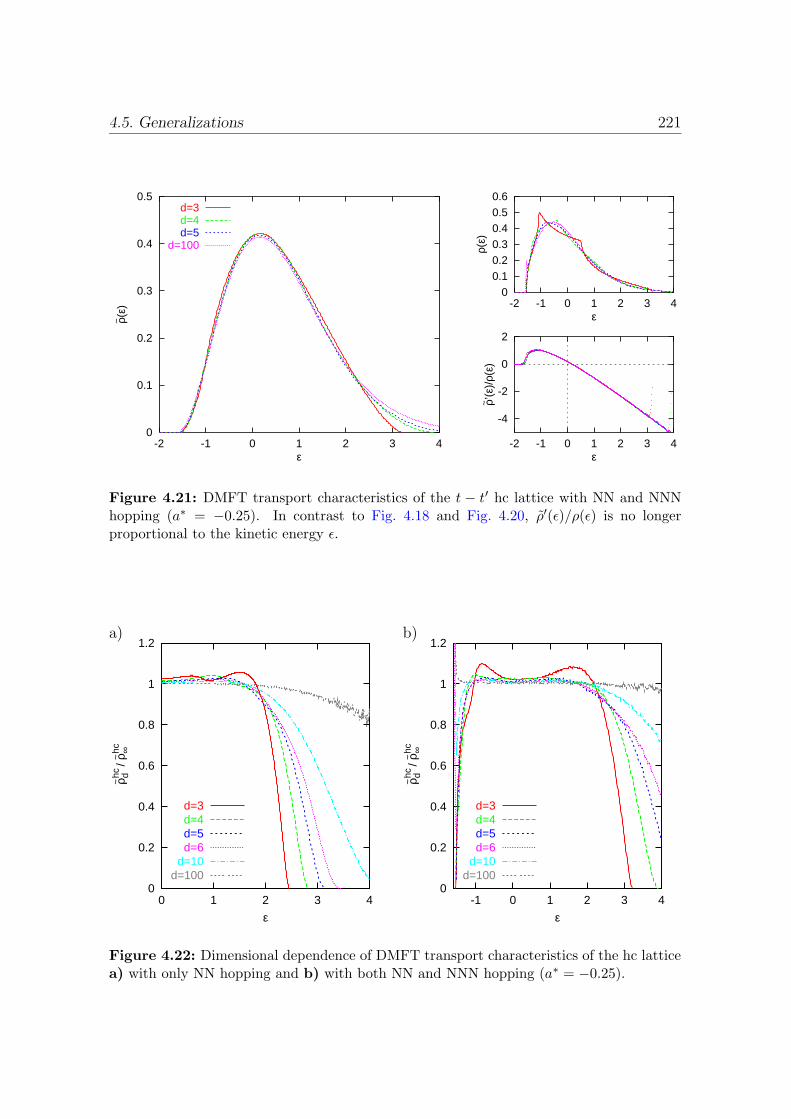
4.5. Generalizations 221
0
0.1
0.2
0.3
0.4
0.5
-2 -1 0 1 2 3 4
~ ρ(ε)
ε
d=3d=4d=5
d=100
00.10.20.30.40.50.6
-2 -1 0 1 2 3 4
ρ(ε)
ε
-4
-2
0
2
-2 -1 0 1 2 3 4
~ ρ’(ε
)/ρ(
ε)
ε
Figure 4.21: DMFT transport characteristics of the t − t′ hc lattice with NN and NNNhopping (a∗ = −0.25). In contrast to Fig. 4.18 and Fig. 4.20, ρ′(ε)/ρ(ε) is no longerproportional to the kinetic energy ε.
a) b)
0
0.2
0.4
0.6
0.8
1
1.2
0 1 2 3 4
~ ρhc d /
~ ρhc ∞
ε
d=3d=4d=5d=6
d=10d=100
0
0.2
0.4
0.6
0.8
1
1.2
-1 0 1 2 3 4
~ ρhc d /
~ ρhc ∞
ε
d=3d=4d=5d=6
d=10d=100
Figure 4.22: Dimensional dependence of DMFT transport characteristics of the hc latticea) with only NN hopping and b) with both NN and NNN hopping (a∗ = −0.25).
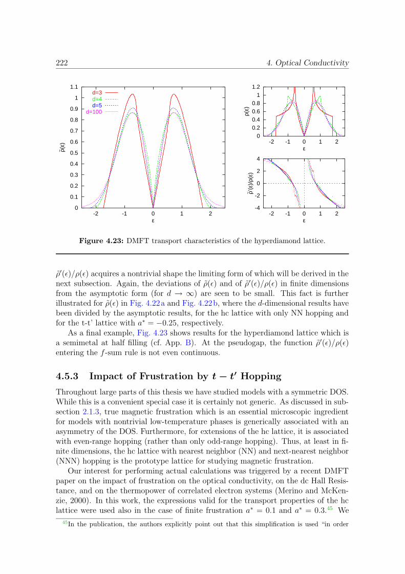
222 4. Optical Conductivity
0
0.1
0.2
0.3
0.4
0.5
0.6
0.7
0.8
0.9
1
1.1
-2 -1 0 1 2
~ ρ(ε)
ε
d=3d=4d=5
d=100
00.20.40.60.8
11.2
-2 -1 0 1 2
ρ(ε)
ε
-4
-2
0
2
4
-2 -1 0 1 2
~ ρ’(ε
)/ρ(
ε)
ε
Figure 4.23: DMFT transport characteristics of the hyperdiamond lattice.
ρ′(ε)/ρ(ε) acquires a nontrivial shape the limiting form of which will be derived in thenext subsection. Again, the deviations of ρ(ε) and of ρ′(ε)/ρ(ε) in finite dimensionsfrom the asymptotic form (for d → ∞) are seen to be small. This fact is furtherillustrated for ρ(ε) in Fig. 4.22a and Fig. 4.22b, where the d-dimensional results havebeen divided by the asymptotic results, for the hc lattice with only NN hopping andfor the t-t’ lattice with a∗ = −0.25, respectively.
As a final example, Fig. 4.23 shows results for the hyperdiamond lattice which isa semimetal at half filling (cf. App. B). At the pseudogap, the function ρ′(ε)/ρ(ε)entering the f -sum rule is not even continuous.
4.5.3 Impact of Frustration by t − t′ Hopping
Throughout large parts of this thesis we have studied models with a symmetric DOS.While this is a convenient special case it is certainly not generic. As discussed in sub-section 2.1.3, true magnetic frustration which is an essential microscopic ingredientfor models with nontrivial low-temperature phases is generically associated with anasymmetry of the DOS. Furthermore, for extensions of the hc lattice, it is associatedwith even-range hopping (rather than only odd-range hopping). Thus, at least in fi-nite dimensions, the hc lattice with nearest neighbor (NN) and next-nearest neighbor(NNN) hopping is the prototype lattice for studying magnetic frustration.
Our interest for performing actual calculations was triggered by a recent DMFTpaper on the impact of frustration on the optical conductivity, on the dc Hall Resis-tance, and on the thermopower of correlated electron systems (Merino and McKen-zie, 2000). In this work, the expressions valid for the transport properties of the hclattice were used also in the case of finite frustration a∗ = 0.1 and a∗ = 0.3.45 We
45In the publication, the authors explicitly point out that this simplification is used “in order

4.5. Generalizations 223
will here derive the correct expressions, i.e., perform the necessary momentum sumsand compare the results to an evaluation of the hc expressions.
In the low-frequency limit of the homogeneous phase, the transverse conductivityreduces to (Shastry, Shraiman, and Singh, 1993; Merino and McKenzie, 2000)46
σxy = σH0
∞∫
−∞
dω∂nf (ω)
∂ω
1
N
∑
k
(∂εk∂kx
)2∂2εk∂k2
y
A3εk
(ω) . (4.140)
Here, σH0 = 4π2|e|3aB/3~
2 and B is the magnetic field in z direction. The spectralfunction Aεk(ω) depends on momentum k only via the free dispersion εk. The dcHall coefficient
RH =σxy
Bσ2xx(ω = 0)
(4.141)
follows from (4.140) and the limit ω → 0 of (4.65). The thermopower is given bythe expression (Schweitzer and Czycholl, 1991; Pruschke, Jarrell, and Freericks, 1995;Merino and McKenzie, 2000)
S = − kB|e|T
L12
L11
(4.142)
where the transport integrals reduce for d→∞ to47
Lij = −∞∫
−∞
dω∂nf (ω)
∂ω
[ 2
N
∑
k
(∂εk∂kx
)2A2εk
(ω)]i
ωj−1 (4.143)
In order to perform the sums over momenta, we will use the fact that the dispersionof the t− t′ lattice may be expressed in terms of the dispersion εhc
k of the hypercubiclattice with unit scaled hopping amplitude t∗ = 1,
ε(k, t∗, a∗) ≡ εk = t∗εhck +
a∗t∗√2
(
1−(εhck
)2)
≡ f(εhck ) . (4.144)
Consequently, we may write
vk,x ≡∂εk∂kx
= t∗(1−√
2 a∗εhck
)∂εhck
∂kx(4.145)
where ∂εhck /∂kx =
√2dsin(kx). Averaging over kx, this yields for the squared Fermi
velocity
〈v2k,x〉(ε) =
t∗2
d
(
1−√
2a∗ε)2∣∣∣∣ε=f(ε)
(4.146)
=1 + 2a∗2 − 2
√2a∗√
1 + a∗2ε
1 + a∗2. (4.147)
to avoid the cumbersome sums over momentum”. They claim it to be justified by their focus “onmany-body effects and not on how different band structures may change the results slightly”.
46In finite dimensions, the second derivative in x direction is supplemented by a term
−(
∂εk
∂ky
)2 ∂2εk
∂kx∂ky(which carries an additional factor 1/d and, therefore, vanishes for d→∞).
47Note that this expression is only approximate since it does not take contributions due to theflow of doubly occupied sites into account (Georges et al., 1996).

224 4. Optical Conductivity
a) b)
0
0.2
0.4
0.6
0.8
1
1.2
1.4
-4 -3 -2 -1 0 1 2 3 4
<|v
k|2 >
, ρ
ε
a*=0a*=-0.1a*=-0.3
a*=-∞
-6
-4
-2
0
2
4
-4 -3 -2 -1 0 1 2 3 4
d <
∂2 ε k/∂
k x2 >
ε
a*=0.0a*=-0.1a*=-0.3a*=-0.5
a*=-∞
Figure 4.24: DMFT transport characteristics of the t− t′ lattice: a) For finite frustration,the squared Fermi velocity 〈|vk|2〉(ε) (thick lines) is not constant, but vanishes linearly at
the band edge of the noninteracting DOS (thin lines). b) d〈 ∂2εk∂k2
x〉(ε) = ρ′(ε)/ρ(ε) needed
for computing the Hall conductivity and the f -sum. Deviations from the linear hc form(a∗ = 0) are most significant near the band edge.
In (4.147) we have already set t∗ =√
1/(1 + a∗2) in order to guarantee unit varianceof the corresponding DOS. Note that the inverse transformation function F−1 is notunique for the t− t′ lattice; this didn’t matter here because both roots correspondingto the same εk also yield the same v2
k,x. As expected on physical grounds, the Fermivelocity vanishes at the band edge. In fact, 〈v2
k,x〉(ε) is proportional the distance fromthe band edge as illustrated in Fig. 4.24 (thick lines). Evidently, the assumption of〈v2
k,x〉(ε) being constant (as implied by the formulas derived for the hc lattice) isbad already for |a∗| = 0.1 and fails completely for stronger frustration |a∗| = 0.3and beyond. In particular, the dependence of transport properties on the degree offrustration may even be dominated by the change in 〈v2
k,x〉(ε).The evaluation of the second derivative is a bit more complicated since here both
roots of F(ε) = ε contribute differently. Therefore, we split the total DOS of thet− t′ lattice
ρ(ε, a∗) =
√2π
1+a∗2
r(ε,a∗)exp
(
− 1+r2(ε,a∗)4a∗2
)
cosh(r(ε,a∗)2a∗2
)
for sign(a∗)ε < r0
0 otherwise ,(4.148)
where r(ε, a∗) =√
1 + 2a∗(a∗ −√
2ε√
1 + a∗2) and where the band edge is given by
r0 = (a∗ + 1/(2a∗))/√
2, into two contributions (with the same boundaries):
ρ±(ε, a∗) =
√
1
2π
1 + a∗2
r(ε, a∗)exp
(
−(1± r(ε, a∗)
)2
4a∗2
)
. (4.149)
Using the notation
h0(ε, a∗) =
1
2a∗2−√
2(a∗ +1
a∗); h±(ε, a∗) =
√2a∗h0(ε, a
∗)±√
1 + h0(ε, a∗)
1 + a∗2
(4.150)
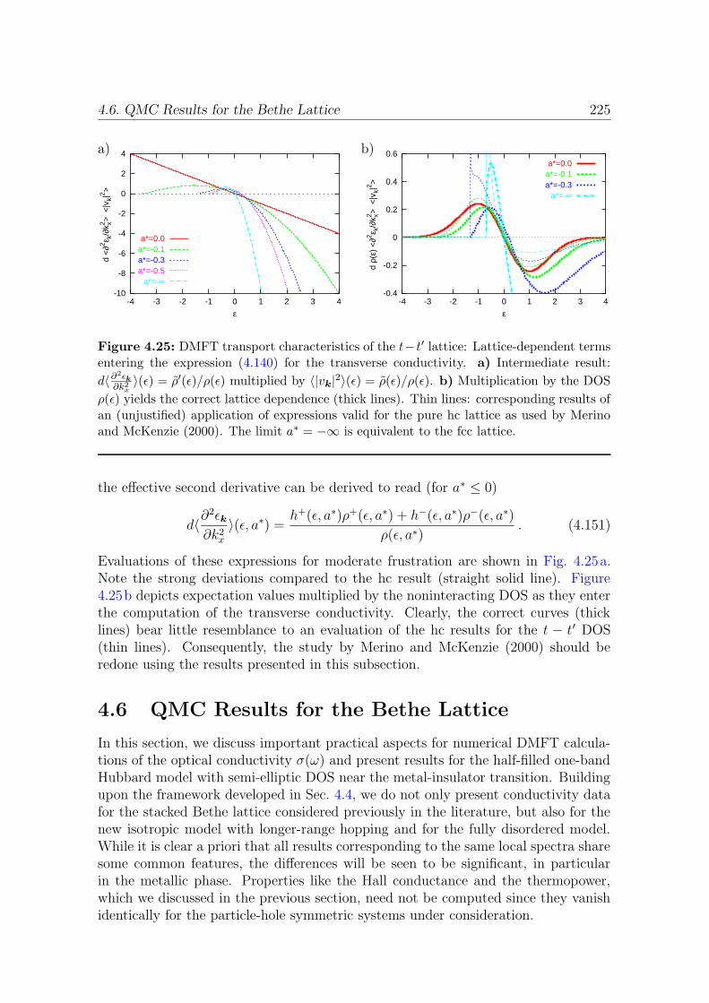
4.6. QMC Results for the Bethe Lattice 225
a) b)
-10
-8
-6
-4
-2
0
2
4
-4 -3 -2 -1 0 1 2 3 4
d <
∂2 ε k/∂
k x2 > <
|vk|
2 >
ε
a*=0.0a*=-0.1a*=-0.3a*=-0.5
a*=-∞-0.4
-0.2
0
0.2
0.4
0.6
-4 -3 -2 -1 0 1 2 3 4
d ρ(
ε) <
∂2 ε k/∂
k x2 > <
|vk|
2 >
ε
a*=0.0a*=-0.1a*=-0.3
a*=-∞
Figure 4.25: DMFT transport characteristics of the t−t′ lattice: Lattice-dependent termsentering the expression (4.140) for the transverse conductivity. a) Intermediate result:
d〈∂2εk∂k2
x〉(ε) = ρ′(ε)/ρ(ε) multiplied by 〈|vk|2〉(ε) = ρ(ε)/ρ(ε). b) Multiplication by the DOS
ρ(ε) yields the correct lattice dependence (thick lines). Thin lines: corresponding results ofan (unjustified) application of expressions valid for the pure hc lattice as used by Merinoand McKenzie (2000). The limit a∗ = −∞ is equivalent to the fcc lattice.
the effective second derivative can be derived to read (for a∗ ≤ 0)
d〈∂2εk∂k2
x
〉(ε, a∗) =h+(ε, a∗)ρ+(ε, a∗) + h−(ε, a∗)ρ−(ε, a∗)
ρ(ε, a∗). (4.151)
Evaluations of these expressions for moderate frustration are shown in Fig. 4.25a.Note the strong deviations compared to the hc result (straight solid line). Figure4.25b depicts expectation values multiplied by the noninteracting DOS as they enterthe computation of the transverse conductivity. Clearly, the correct curves (thicklines) bear little resemblance to an evaluation of the hc results for the t − t′ DOS(thin lines). Consequently, the study by Merino and McKenzie (2000) should beredone using the results presented in this subsection.
4.6 QMC Results for the Bethe Lattice
In this section, we discuss important practical aspects for numerical DMFT calcula-tions of the optical conductivity σ(ω) and present results for the half-filled one-bandHubbard model with semi-elliptic DOS near the metal-insulator transition. Buildingupon the framework developed in Sec. 4.4, we do not only present conductivity datafor the stacked Bethe lattice considered previously in the literature, but also for thenew isotropic model with longer-range hopping and for the fully disordered model.While it is clear a priori that all results corresponding to the same local spectra sharesome common features, the differences will be seen to be significant, in particularin the metallic phase. Properties like the Hall conductance and the thermopower,which we discussed in the previous section, need not be computed since they vanishidentically for the particle-hole symmetric systems under consideration.
226 4. Optical Conductivity
4.6.1 Numerical Procedure for QMC Data
Within the DMFT framework, the optical conductivity may be expressed in thecoherent case48 as [see (4.64) - (4.67)]
Re σxx(ω) = σ0
∞∫
−∞
dε ρxx(ε)
∞∫
−∞
dω′Aε(ω′)Aε(ω
′ + ω)nf(ω
′)− nf(ω + ω′)
ω, (4.152)
where σ0 = 2πe2
~2NV
and nf(ω) =(1 + eβ(ω−µ)
)−1. Evidently, practical calculations
require two basic ingredients: ρxx(ε) = 1N
∑
k v2kxδ(ε− εk) measures the noninteract-
ing density of states weighted with the squared Fermi velocity and thus contains allnecessary information about the lattice. For a given model (characterized by its lat-tice topology and hopping parameters), this function can be determined once and forall, independent of temperature and interaction. For lattices with semi-elliptic BetheDOS, this task was solved in Sec. 4.4. The remaining problem is the computationof the “momentum-dependent” (i.e., dependent on the noninteracting dispersion ε)interacting spectral function
Aε(ω) = − 1
πImGε(ω) , (4.153)
where
Gε(ω) =1
ω − ε− Σ(ω). (4.154)
An evaluation for real frequencies ω yields
Aε(ω) = − 1
π
Im Σ(ω)(ω − ε− Re Σ(ω)
)2+(Im Σ(ω)
)2 . (4.155)
Once Σ(ω) is known on the real axis, the computation of σ(ω) reduces to the eval-uation of a two-dimensional integral (over the variables ε and ω ′). Note that the“momentum”-dependent spectral functions Aε(ω) are strongly peaked in the metallicphase (where |Im Σ(ω)| is small for ω ≈ 0; cf. Fig. 4.29) which can in principle causenumerical instabilities; still, this step is straightforward.
In the context of QMC calculations, the real-frequency self-energy Σ(ω) has tobe extracted in a multi-step procedure49 which is summarized in Fig. 4.26 and willbe discussed in the remainder of this subsection. All steps will be illustrated onthe basis of the spectral function of the Hubbard model with semi-elliptic DOS atT = 0.05 and U = 4.0 shown as solid line in Fig. 3.77 in Sec. 3.8 (resulting from QMCusing ∆τ = 0.1 and MEM using a flat default model). The corresponding imaginarypart of the real-frequency Green function is indicated by circles in Fig. 4.27. It willbecome apparent later that the frequency grid ∆ω = 0.1 used in the MEM procedure
48For the cases of disorder or a single-link topology which imply incoherent transport, see sub-section 4.4.2 and the results presented in subsection 4.6.3.
49The QMC method itself and the MEM determination of the local spectral function A(ω) =− 1
π ImG(ω) have already been discussed in Sec. 1.3, Sec. 1.4, and Sec. 3.8.
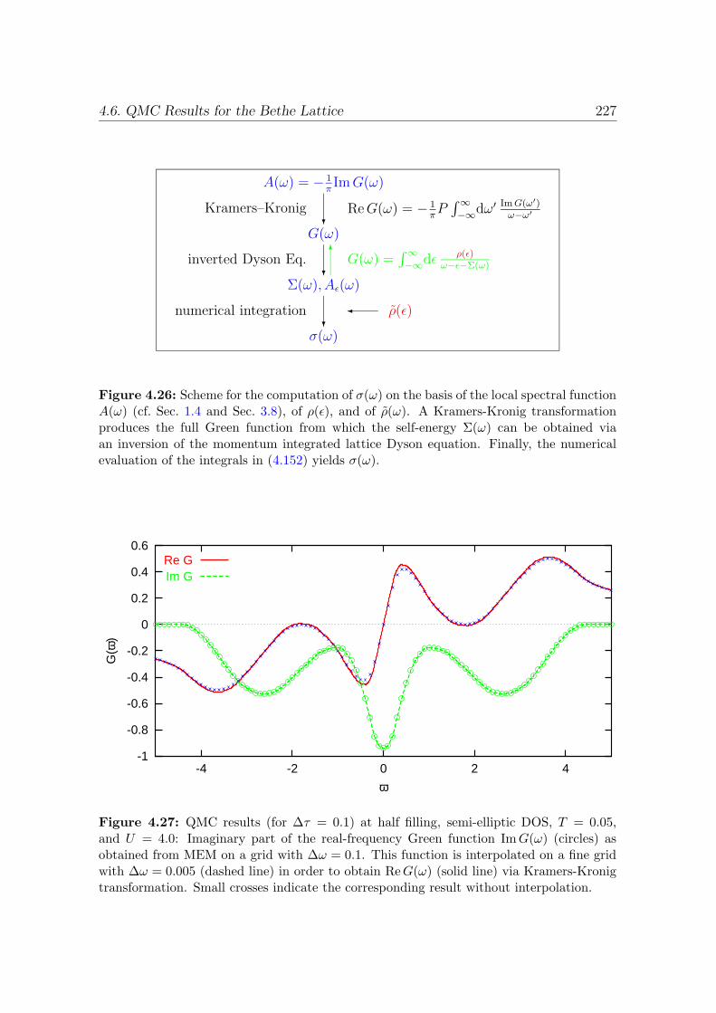
4.6. QMC Results for the Bethe Lattice 227
?
?
?
A(ω) = − 1πImG(ω)
G(ω)
Σ(ω), Aε(ω)
σ(ω)
Kramers–Kronig
inverted Dyson Eq.
numerical integration ¾ ρ(ε)
6 G(ω) =∫∞−∞dε ρ(ε)
ω−ε−Σ(ω)
ReG(ω) = − 1πP∫∞−∞dω′ ImG(ω′)
ω−ω′
Figure 4.26: Scheme for the computation of σ(ω) on the basis of the local spectral functionA(ω) (cf. Sec. 1.4 and Sec. 3.8), of ρ(ε), and of ρ(ω). A Kramers-Kronig transformationproduces the full Green function from which the self-energy Σ(ω) can be obtained viaan inversion of the momentum integrated lattice Dyson equation. Finally, the numericalevaluation of the integrals in (4.152) yields σ(ω).
-1
-0.8
-0.6
-0.4
-0.2
0
0.2
0.4
0.6
-4 -2 0 2 4
G(ω
)
ω
Re GIm G
Figure 4.27: QMC results (for ∆τ = 0.1) at half filling, semi-elliptic DOS, T = 0.05,and U = 4.0: Imaginary part of the real-frequency Green function ImG(ω) (circles) asobtained from MEM on a grid with ∆ω = 0.1. This function is interpolated on a fine gridwith ∆ω = 0.005 (dashed line) in order to obtain ReG(ω) (solid line) via Kramers-Kronigtransformation. Small crosses indicate the corresponding result without interpolation.
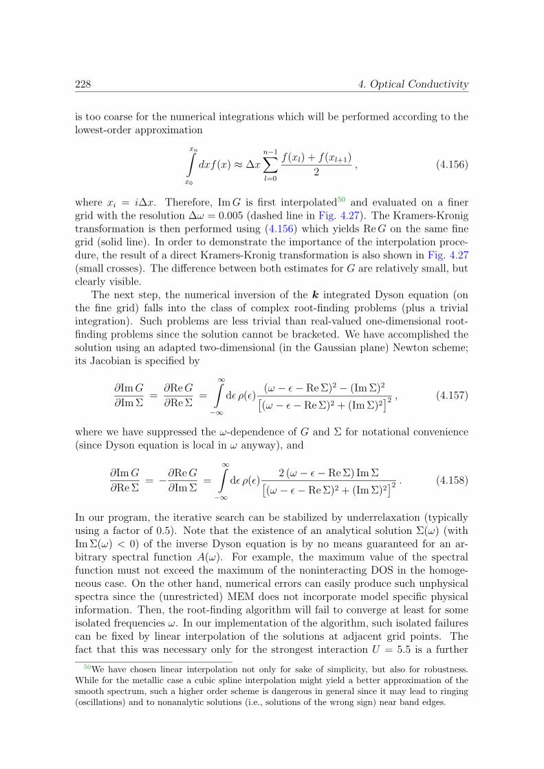
228 4. Optical Conductivity
is too coarse for the numerical integrations which will be performed according to thelowest-order approximation
xn∫
x0
dxf(x) ≈ ∆xn−1∑
l=0
f(xl) + f(xl+1)
2, (4.156)
where xi = i∆x. Therefore, ImG is first interpolated50 and evaluated on a finergrid with the resolution ∆ω = 0.005 (dashed line in Fig. 4.27). The Kramers-Kronigtransformation is then performed using (4.156) which yields ReG on the same finegrid (solid line). In order to demonstrate the importance of the interpolation proce-dure, the result of a direct Kramers-Kronig transformation is also shown in Fig. 4.27(small crosses). The difference between both estimates for G are relatively small, butclearly visible.
The next step, the numerical inversion of the k integrated Dyson equation (onthe fine grid) falls into the class of complex root-finding problems (plus a trivialintegration). Such problems are less trivial than real-valued one-dimensional root-finding problems since the solution cannot be bracketed. We have accomplished thesolution using an adapted two-dimensional (in the Gaussian plane) Newton scheme;its Jacobian is specified by
∂ImG
∂Im Σ=
∂ReG
∂Re Σ=
∞∫
−∞
dε ρ(ε)(ω − ε− Re Σ)2 − (Im Σ)2
[(ω − ε− Re Σ)2 + (Im Σ)2
]2 , (4.157)
where we have suppressed the ω-dependence of G and Σ for notational convenience(since Dyson equation is local in ω anyway), and
∂ImG
∂Re Σ= −∂ReG
∂Im Σ=
∞∫
−∞
dε ρ(ε)2 (ω − ε− Re Σ) Im Σ
[(ω − ε− Re Σ)2 + (Im Σ)2
]2 . (4.158)
In our program, the iterative search can be stabilized by underrelaxation (typicallyusing a factor of 0.5). Note that the existence of an analytical solution Σ(ω) (withIm Σ(ω) < 0) of the inverse Dyson equation is by no means guaranteed for an ar-bitrary spectral function A(ω). For example, the maximum value of the spectralfunction must not exceed the maximum of the noninteracting DOS in the homoge-neous case. On the other hand, numerical errors can easily produce such unphysicalspectra since the (unrestricted) MEM does not incorporate model specific physicalinformation. Then, the root-finding algorithm will fail to converge at least for someisolated frequencies ω. In our implementation of the algorithm, such isolated failurescan be fixed by linear interpolation of the solutions at adjacent grid points. Thefact that this was necessary only for the strongest interaction U = 5.5 is a further
50We have chosen linear interpolation not only for sake of simplicity, but also for robustness.While for the metallic case a cubic spline interpolation might yield a better approximation of thesmooth spectrum, such a higher order scheme is dangerous in general since it may lead to ringing(oscillations) and to nonanalytic solutions (i.e., solutions of the wrong sign) near band edges.
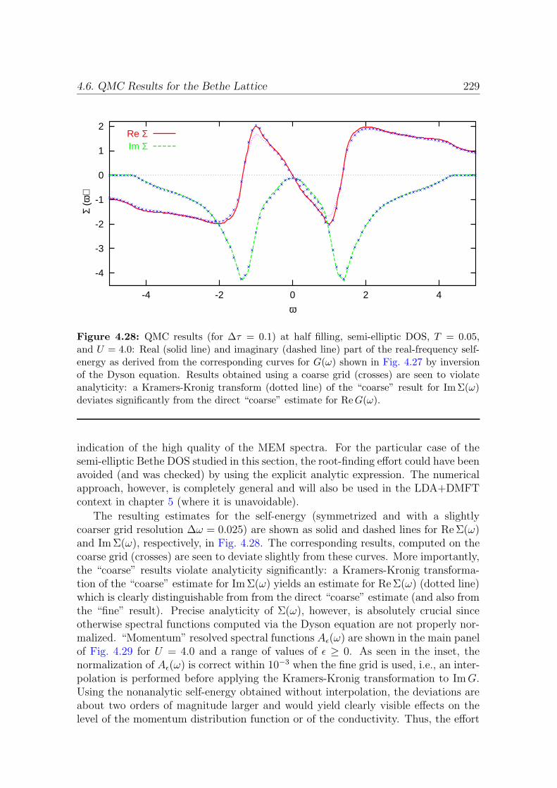
4.6. QMC Results for the Bethe Lattice 229
-4
-3
-2
-1
0
1
2
-4 -2 0 2 4
Σ (ω
)
ω
Re ΣIm Σ
Figure 4.28: QMC results (for ∆τ = 0.1) at half filling, semi-elliptic DOS, T = 0.05,and U = 4.0: Real (solid line) and imaginary (dashed line) part of the real-frequency self-energy as derived from the corresponding curves for G(ω) shown in Fig. 4.27 by inversionof the Dyson equation. Results obtained using a coarse grid (crosses) are seen to violateanalyticity: a Kramers-Kronig transform (dotted line) of the “coarse” result for ImΣ(ω)deviates significantly from the direct “coarse” estimate for ReG(ω).
indication of the high quality of the MEM spectra. For the particular case of thesemi-elliptic Bethe DOS studied in this section, the root-finding effort could have beenavoided (and was checked) by using the explicit analytic expression. The numericalapproach, however, is completely general and will also be used in the LDA+DMFTcontext in chapter 5 (where it is unavoidable).
The resulting estimates for the self-energy (symmetrized and with a slightlycoarser grid resolution ∆ω = 0.025) are shown as solid and dashed lines for Re Σ(ω)and Im Σ(ω), respectively, in Fig. 4.28. The corresponding results, computed on thecoarse grid (crosses) are seen to deviate slightly from these curves. More importantly,the “coarse” results violate analyticity significantly: a Kramers-Kronig transforma-tion of the “coarse” estimate for Im Σ(ω) yields an estimate for Re Σ(ω) (dotted line)which is clearly distinguishable from from the direct “coarse” estimate (and also fromthe “fine” result). Precise analyticity of Σ(ω), however, is absolutely crucial sinceotherwise spectral functions computed via the Dyson equation are not properly nor-malized. “Momentum” resolved spectral functions Aε(ω) are shown in the main panelof Fig. 4.29 for U = 4.0 and a range of values of ε ≥ 0. As seen in the inset, thenormalization of Aε(ω) is correct within 10−3 when the fine grid is used, i.e., an inter-polation is performed before applying the Kramers-Kronig transformation to ImG.Using the nonanalytic self-energy obtained without interpolation, the deviations areabout two orders of magnitude larger and would yield clearly visible effects on thelevel of the momentum distribution function or of the conductivity. Thus, the effort
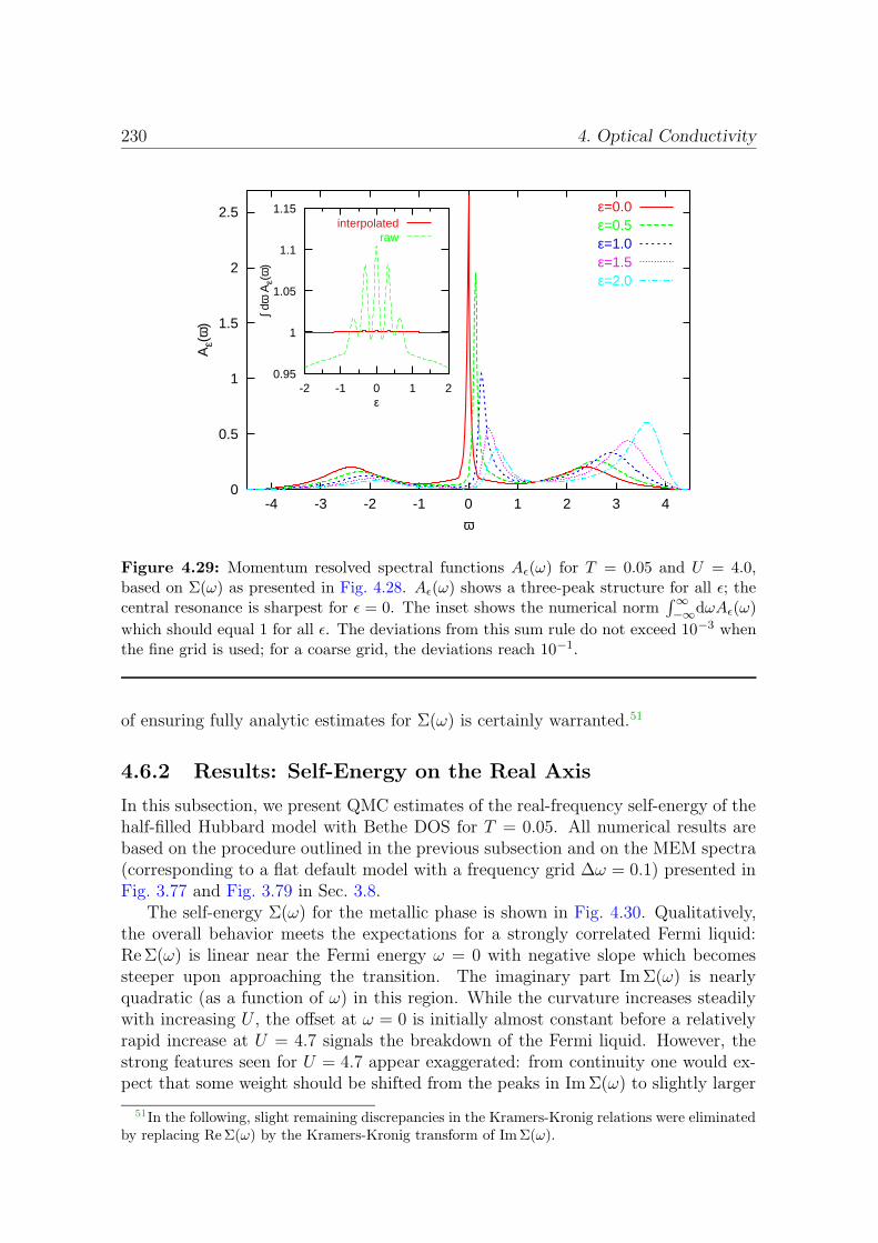
230 4. Optical Conductivity
0
0.5
1
1.5
2
2.5
-4 -3 -2 -1 0 1 2 3 4
Aε(
ω)
ω
ε=0.0ε=0.5ε=1.0ε=1.5ε=2.0
0.95
1
1.05
1.1
1.15
-2 -1 0 1 2
∫ dω
Aε(
ω)
ε
interpolatedraw
Figure 4.29: Momentum resolved spectral functions Aε(ω) for T = 0.05 and U = 4.0,based on Σ(ω) as presented in Fig. 4.28. Aε(ω) shows a three-peak structure for all ε; thecentral resonance is sharpest for ε = 0. The inset shows the numerical norm
∫∞−∞dωAε(ω)
which should equal 1 for all ε. The deviations from this sum rule do not exceed 10−3 whenthe fine grid is used; for a coarse grid, the deviations reach 10−1.
of ensuring fully analytic estimates for Σ(ω) is certainly warranted.51
4.6.2 Results: Self-Energy on the Real Axis
In this subsection, we present QMC estimates of the real-frequency self-energy of thehalf-filled Hubbard model with Bethe DOS for T = 0.05. All numerical results arebased on the procedure outlined in the previous subsection and on the MEM spectra(corresponding to a flat default model with a frequency grid ∆ω = 0.1) presented inFig. 3.77 and Fig. 3.79 in Sec. 3.8.
The self-energy Σ(ω) for the metallic phase is shown in Fig. 4.30. Qualitatively,the overall behavior meets the expectations for a strongly correlated Fermi liquid:Re Σ(ω) is linear near the Fermi energy ω = 0 with negative slope which becomessteeper upon approaching the transition. The imaginary part Im Σ(ω) is nearlyquadratic (as a function of ω) in this region. While the curvature increases steadilywith increasing U , the offset at ω = 0 is initially almost constant before a relativelyrapid increase at U = 4.7 signals the breakdown of the Fermi liquid. However, thestrong features seen for U = 4.7 appear exaggerated: from continuity one would ex-pect that some weight should be shifted from the peaks in Im Σ(ω) to slightly larger
51In the following, slight remaining discrepancies in the Kramers-Kronig relations were eliminatedby replacing ReΣ(ω) by the Kramers-Kronig transform of Im Σ(ω).
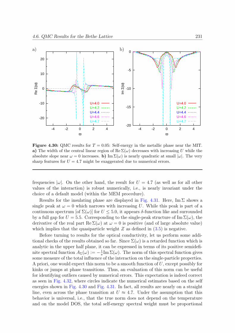
4.6. QMC Results for the Bethe Lattice 231
a) b)
-20
-10
0
10
20
-4 -2 0 2 4
Re
Σ(ω
)
ω
U=4.0U=4.2U=4.4U=4.6U=4.7
-20
-15
-10
-5
0
-4 -2 0 2 4
Im Σ
(ω)
ω
U=4.0U=4.2U=4.4U=4.6U=4.7
Figure 4.30: QMC results for T = 0.05: Self-energy in the metallic phase near the MIT.a) The width of the central linear region of Re Σ(ω) decreases with increasing U while theabsolute slope near ω = 0 increases. b) Im Σ(ω) is nearly quadratic at small |ω|. The verysharp features for U = 4.7 might be exaggerated due to numerical errors.
frequencies |ω|. On the other hand, the result for U = 4.7 (as well as for all othervalues of the interaction) is robust numerically, i.e., is nearly invariant under thechoice of a default model (within the MEM procedure).
Results for the insulating phase are displayed in Fig. 4.31. Here, Im Σ shows asingle peak at ω = 0 which narrows with increasing U . While this peak is part of acontinuous spectrum [of Σ(ω)] for U ≤ 5.0, it appears δ-function like and surroundedby a full gap for U = 5.5. Corresponding to the single-peak structure of Im Σ(ω), thederivative of the real part Re Σ(ω) at ω = 0 is positive (and of large absolute value)which implies that the quasiparticle weight Z as defined in (3.5) is negative.
Before turning to results for the optical conductivity, let us perform some addi-tional checks of the results obtained so far. Since Σ(ω) is a retarded function which isanalytic in the upper half plane, it can be expressed in terms of its positive semidefi-nite spectral function AΣ(ω) := − 1
πIm Σ(ω). The norm of this spectral function gives
some measure of the total influence of the interaction on the single-particle properties.A priori, one would expect this norm to be a smooth function of U , except possibly forkinks or jumps at phase transitions. Thus, an evaluation of this norm can be usefulfor identifying outliers caused by numerical errors. This expectation is indeed correctas seen in Fig. 4.32, where circles indicate the numerical estimates based on the selfenergies shown in Fig. 4.30 and Fig. 4.31. In fact, all results are nearly on a straightline, even across the phase transition at U ≈ 4.7. Under the assumption that thisbehavior is universal, i.e., that the true norm does not depend on the temperatureand on the model DOS, the total self-energy spectral weight must be proportional
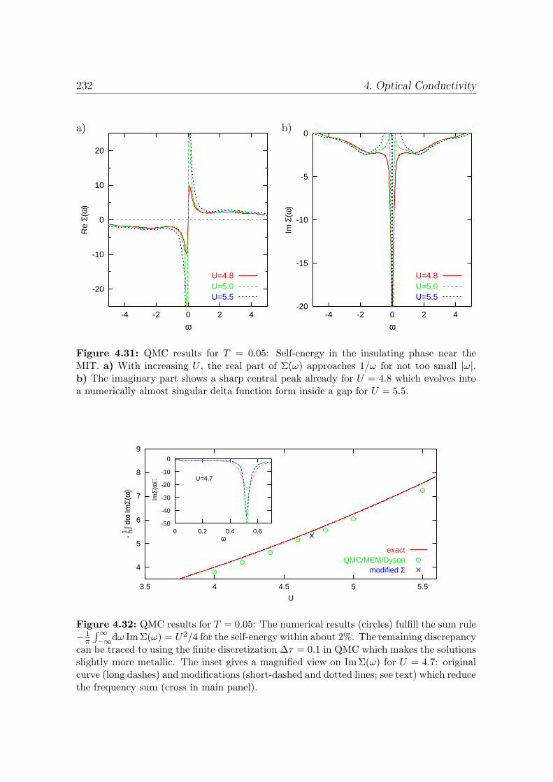
232 4. Optical Conductivity
a) b)
-20
-10
0
10
20
-4 -2 0 2 4
Re
Σ(ω
)
ω
U=4.8U=5.0U=5.5
-20
-15
-10
-5
0
-4 -2 0 2 4
Im Σ
(ω)
ω
U=4.8U=5.0U=5.5
Figure 4.31: QMC results for T = 0.05: Self-energy in the insulating phase near theMIT. a) With increasing U , the real part of Σ(ω) approaches 1/ω for not too small |ω|.b) The imaginary part shows a sharp central peak already for U = 4.8 which evolves intoa numerically almost singular delta function form inside a gap for U = 5.5.
4
5
6
7
8
9
3.5 4 4.5 5 5.5
- 1 π-
∫ dω
ImΣ(
ω)
U
exactQMC/MEM/Dyson
modified Σ
-50
-40
-30
-20
-10
0
0 0.2 0.4 0.6
ImΣ(
ω)
ω
U=4.7
Figure 4.32: QMC results for T = 0.05: The numerical results (circles) fulfill the sum rule− 1π
∫∞−∞dω Im Σ(ω) = U2/4 for the self-energy within about 2%. The remaining discrepancy
can be traced to using the finite discretization ∆τ = 0.1 in QMC which makes the solutionsslightly more metallic. The inset gives a magnified view on Im Σ(ω) for U = 4.7: originalcurve (long dashes) and modifications (short-dashed and dotted lines; see text) which reducethe frequency sum (cross in main panel).
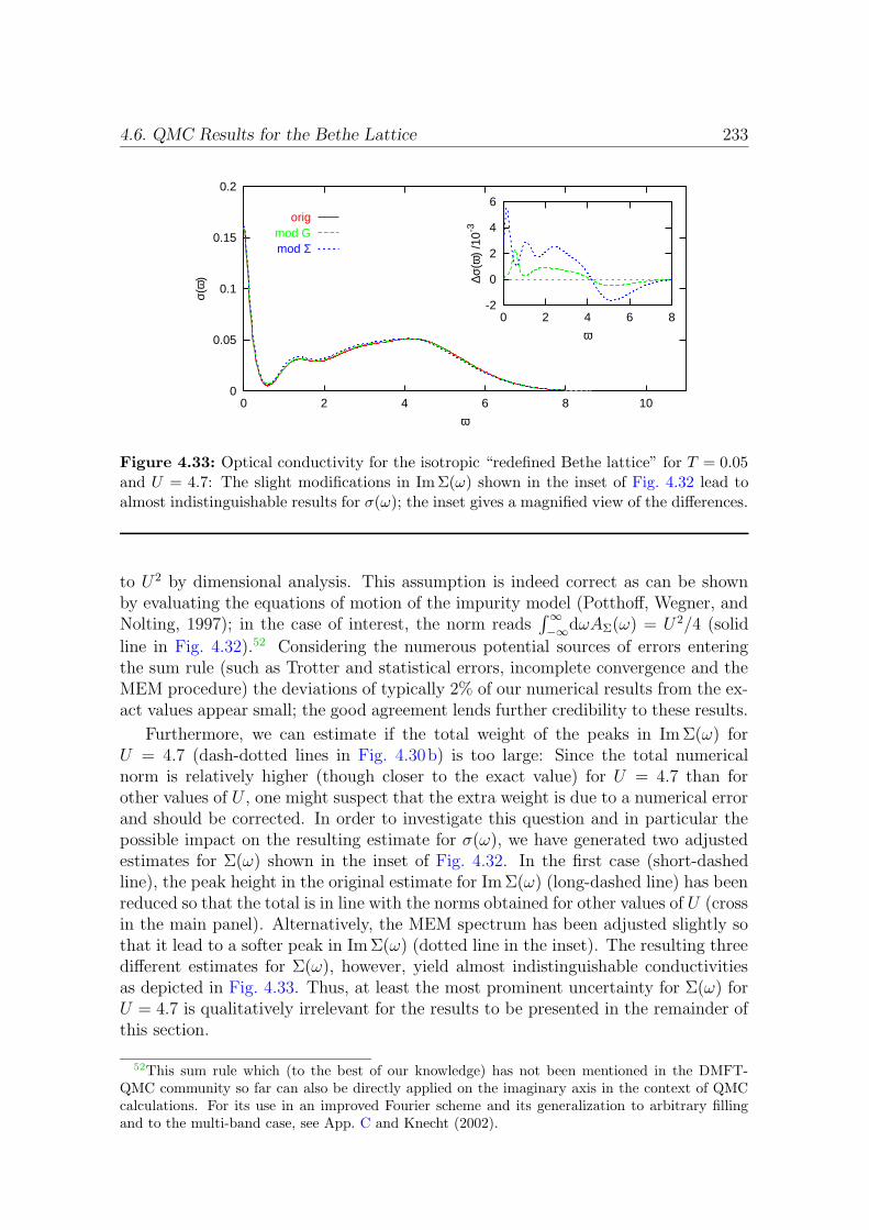
4.6. QMC Results for the Bethe Lattice 233
0
0.05
0.1
0.15
0.2
0 2 4 6 8 10
σ(ω
)
ω
origmod Gmod Σ
-2
0
2
4
6
0 2 4 6 8
∆σ(ω
) /1
0-3
ω
Figure 4.33: Optical conductivity for the isotropic “redefined Bethe lattice” for T = 0.05and U = 4.7: The slight modifications in Im Σ(ω) shown in the inset of Fig. 4.32 lead toalmost indistinguishable results for σ(ω); the inset gives a magnified view of the differences.
to U 2 by dimensional analysis. This assumption is indeed correct as can be shownby evaluating the equations of motion of the impurity model (Potthoff, Wegner, andNolting, 1997); in the case of interest, the norm reads
∫∞−∞dωAΣ(ω) = U 2/4 (solid
line in Fig. 4.32).52 Considering the numerous potential sources of errors enteringthe sum rule (such as Trotter and statistical errors, incomplete convergence and theMEM procedure) the deviations of typically 2% of our numerical results from the ex-act values appear small; the good agreement lends further credibility to these results.
Furthermore, we can estimate if the total weight of the peaks in Im Σ(ω) forU = 4.7 (dash-dotted lines in Fig. 4.30b) is too large: Since the total numericalnorm is relatively higher (though closer to the exact value) for U = 4.7 than forother values of U , one might suspect that the extra weight is due to a numerical errorand should be corrected. In order to investigate this question and in particular thepossible impact on the resulting estimate for σ(ω), we have generated two adjustedestimates for Σ(ω) shown in the inset of Fig. 4.32. In the first case (short-dashedline), the peak height in the original estimate for Im Σ(ω) (long-dashed line) has beenreduced so that the total is in line with the norms obtained for other values of U (crossin the main panel). Alternatively, the MEM spectrum has been adjusted slightly sothat it lead to a softer peak in Im Σ(ω) (dotted line in the inset). The resulting threedifferent estimates for Σ(ω), however, yield almost indistinguishable conductivitiesas depicted in Fig. 4.33. Thus, at least the most prominent uncertainty for Σ(ω) forU = 4.7 is qualitatively irrelevant for the results to be presented in the remainder ofthis section.
52This sum rule which (to the best of our knowledge) has not been mentioned in the DMFT-QMC community so far can also be directly applied on the imaginary axis in the context of QMCcalculations. For its use in an improved Fourier scheme and its generalization to arbitrary fillingand to the multi-band case, see App. C and Knecht (2002).

234 4. Optical Conductivity
0
0.05
0.1
0.15
0.2
0 1 2 3 4 5 6 7 8
σ(ω
)
ω
U=4.0U=4.2U=4.4U=4.6U=4.7
0
0.1
0.2
0.3
0.4
0 1 2 3 4 5 6 7 8
∫ 0ω d
ω’ σ
(ω’)
ω
Figure 4.34: Optical conductivity σ(ω) for the isotropic “redefined Bethe lattice” at T =0.05 in the metallic phase. With increasing U , weight is shifted from a Drude peak at ω ≈ 0to a mid-infrared peak/shoulder at ω ≈ U/2 and, finally, to a broad incoherent peak atω ≈ U . The inset shows the partial f -sum
∫ ω0 dω′σ(ω′) which saturates for ω ≈ 8.
4.6.3 Results: Optical Conductivity
This subsection comprises the main numerical results of this chapter. Using theprocedures detailed in the previous subsection, we will here present results in theparamagnetic low-temperature phase near the Mott metal-insulator transition. Theoptical conductivity data will in turn be shown for three different definitions, i.e.,different models compatible with a semi-elliptic DOS: first, the isotropic “redefinedBethe lattice” specified in Sec. 2.4 (using the general dispersion approach developedin Sec. 2.3), then the (anisotropic) stacked Bethe lattice, and, finally, the incoherentdefinition which corresponds to a disordered model or to a single-chain layout of theBethe lattice. The numerical results for the first two cases will be based on the self-energies Σ(ω) shown in Fig. 4.30 and Fig. 4.31. An estimate of the self-energy is notneeded in the last, incoherent case; here, the optical conductivity will be computeddirectly from the MEM spectra A(ω) shown in Fig. 3.77 and Fig. 3.79. In all cases,the constants e, ~, and the lattice spacing a are set to unity which corresponds tosetting σ0 = 2π [for the coherent case; cf. (4.67)].
Coherent Transport
We start the presentation of optical conductivity data with the redefined Bethe lat-tice; for this model, ρ(ω) has the exact analytic expression (4.133). Figure 4.34displays results for the metallic phase near the MIT. Each curve features a promi-nent “Drude” peak at low frequencies which is associated with excitations within
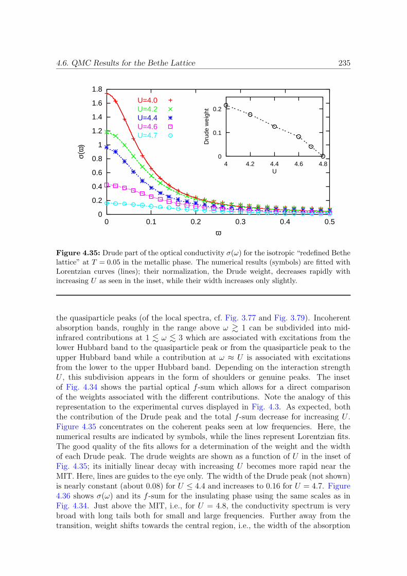
4.6. QMC Results for the Bethe Lattice 235
0
0.2
0.4
0.6
0.8
1
1.2
1.4
1.6
1.8
0 0.1 0.2 0.3 0.4 0.5
σ(ω
)
ω
U=4.0U=4.2U=4.4U=4.6U=4.7
0
0.1
0.2
4 4.2 4.4 4.6 4.8
Dru
de w
eigh
t
U
Figure 4.35: Drude part of the optical conductivity σ(ω) for the isotropic “redefined Bethelattice” at T = 0.05 in the metallic phase. The numerical results (symbols) are fitted withLorentzian curves (lines); their normalization, the Drude weight, decreases rapidly withincreasing U as seen in the inset, while their width increases only slightly.
the quasiparticle peaks (of the local spectra, cf. Fig. 3.77 and Fig. 3.79). Incoherentabsorption bands, roughly in the range above ω & 1 can be subdivided into mid-infrared contributions at 1 . ω . 3 which are associated with excitations from thelower Hubbard band to the quasiparticle peak or from the quasiparticle peak to theupper Hubbard band while a contribution at ω ≈ U is associated with excitationsfrom the lower to the upper Hubbard band. Depending on the interaction strengthU , this subdivision appears in the form of shoulders or genuine peaks. The insetof Fig. 4.34 shows the partial optical f -sum which allows for a direct comparisonof the weights associated with the different contributions. Note the analogy of thisrepresentation to the experimental curves displayed in Fig. 4.3. As expected, boththe contribution of the Drude peak and the total f -sum decrease for increasing U .Figure 4.35 concentrates on the coherent peaks seen at low frequencies. Here, thenumerical results are indicated by symbols, while the lines represent Lorentzian fits.The good quality of the fits allows for a determination of the weight and the widthof each Drude peak. The drude weights are shown as a function of U in the inset ofFig. 4.35; its initially linear decay with increasing U becomes more rapid near theMIT. Here, lines are guides to the eye only. The width of the Drude peak (not shown)is nearly constant (about 0.08) for U ≤ 4.4 and increases to 0.16 for U = 4.7. Figure4.36 shows σ(ω) and its f -sum for the insulating phase using the same scales as inFig. 4.34. Just above the MIT, i.e., for U = 4.8, the conductivity spectrum is verybroad with long tails both for small and large frequencies. Further away from thetransition, weight shifts towards the central region, i.e., the width of the absorption

236 4. Optical Conductivity
0
0.05
0.1
0.15
0.2
0 1 2 3 4 5 6 7 8
σ(ω
)
ω
U=4.8U=5.0U=5.5
0
0.1
0.2
0.3
0.4
0 1 2 3 4 5 6 7 8
∫ 0ω d
ω’ σ
(ω’)
ω
Figure 4.36: Optical conductivity σ(ω) for the isotropic “redefined Bethe lattice” at T =0.05 in the insulating phase. The inset shows the partial f -sum (cf. Fig. 4.34).
band shrinks slightly (by about 15% from U = 4.8 to U = 5.5).In the following, plots analogous to the last three figures will be shown (using
the same scales) for the stacked Bethe lattice discussed in subsection 4.4.3. Fornotational simplicity, we will continue to write σ(ω) instead of using the notationσxx(ω) appropriate for an anisotropic model. We expect to find qualitatively verysimilar results as for the isotropic model considered before; still the differences willbe seen to be significant. In fact, Fig. 4.37 and Fig. 4.38 demonstrate that within themetallic phase both the Drude weights and the total f -sums are reduced significantlycompared with the isotropic case. The widths of the Drude peaks, however, are nearlyidentical. No significant changes are observed in the insulating phase in Fig. 4.39 upto a slight reduction in the total f -sum.
Incoherent Transport
Completely incoherent transport follows both from Stumpf’s single-chain view of theBethe lattice detailed in subsection 4.4.2 and from offdiagonal disorder as discussed insubsection 4.4.4. We will here consider the disordered case which yields an extensiveconductivity. The formal expression (4.132) reads for the paramagnetic phase andthe choice of units specified above
σxx(ω) = 2π
∞∫
−∞
dω′A(ω′)A(ω′ + ω)nf(ω
′)− nf(ω′ + ω)
ω. (4.159)
The primary new feature seen in Fig. 4.40 and Fig. 4.41 for the metallic phase is
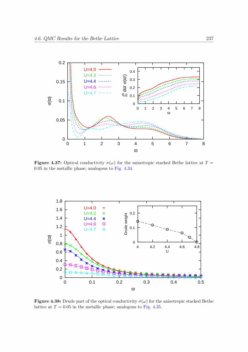
4.6. QMC Results for the Bethe Lattice 237
0
0.05
0.1
0.15
0.2
0 1 2 3 4 5 6 7 8
σ(ω
)
ω
U=4.0U=4.2U=4.4U=4.6U=4.7
0
0.1
0.2
0.3
0.4
0 1 2 3 4 5 6 7 8
∫ 0ω d
ω’ σ
(ω’)
ω
Figure 4.37: Optical conductivity σ(ω) for the anisotropic stacked Bethe lattice at T =0.05 in the metallic phase; analogous to Fig. 4.34.
0
0.2
0.4
0.6
0.8
1
1.2
1.4
1.6
1.8
0 0.1 0.2 0.3 0.4 0.5
σ(ω
)
ω
U=4.0U=4.2U=4.4U=4.6U=4.7
0
0.1
0.2
4 4.2 4.4 4.6 4.8
Dru
de w
eigh
t
U
Figure 4.38: Drude part of the optical conductivity σ(ω) for the anisotropic stacked Bethelattice at T = 0.05 in the metallic phase; analogous to Fig. 4.35.
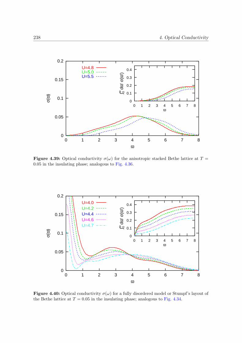
238 4. Optical Conductivity
0
0.05
0.1
0.15
0.2
0 1 2 3 4 5 6 7 8
σ(ω
)
ω
U=4.8U=5.0U=5.5
0
0.1
0.2
0.3
0.4
0 1 2 3 4 5 6 7 8
∫ 0ω d
ω’ σ
(ω’)
ω
Figure 4.39: Optical conductivity σ(ω) for the anisotropic stacked Bethe lattice at T =0.05 in the insulating phase; analogous to Fig. 4.36.
0
0.05
0.1
0.15
0.2
0 1 2 3 4 5 6 7 8
σ(ω
)
ω
U=4.0U=4.2U=4.4U=4.6U=4.7
0
0.1
0.2
0.3
0.4
0 1 2 3 4 5 6 7 8
∫ 0ω d
ω’ σ
(ω’)
ω
Figure 4.40: Optical conductivity σ(ω) for a fully disordered model or Stumpf’s layout ofthe Bethe lattice at T = 0.05 in the insulating phase; analogous to Fig. 4.34.
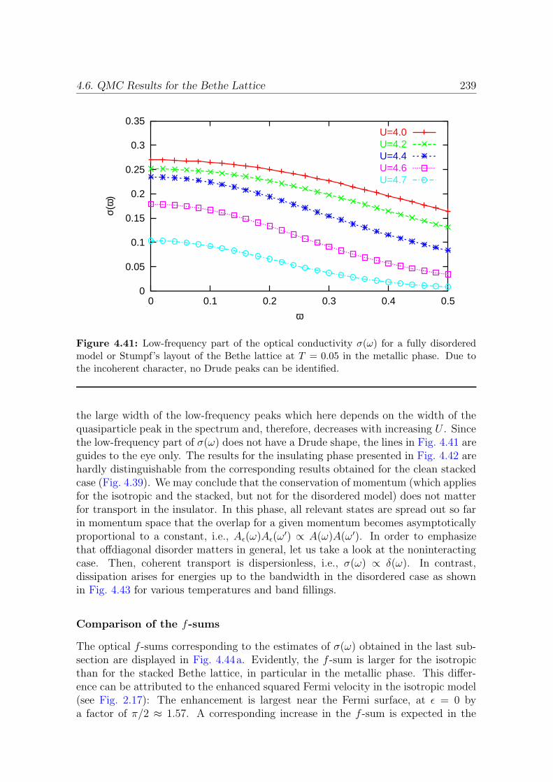
4.6. QMC Results for the Bethe Lattice 239
0
0.05
0.1
0.15
0.2
0.25
0.3
0.35
0 0.1 0.2 0.3 0.4 0.5
σ(ω
)
ω
U=4.0U=4.2U=4.4U=4.6U=4.7
Figure 4.41: Low-frequency part of the optical conductivity σ(ω) for a fully disorderedmodel or Stumpf’s layout of the Bethe lattice at T = 0.05 in the metallic phase. Due tothe incoherent character, no Drude peaks can be identified.
the large width of the low-frequency peaks which here depends on the width of thequasiparticle peak in the spectrum and, therefore, decreases with increasing U . Sincethe low-frequency part of σ(ω) does not have a Drude shape, the lines in Fig. 4.41 areguides to the eye only. The results for the insulating phase presented in Fig. 4.42 arehardly distinguishable from the corresponding results obtained for the clean stackedcase (Fig. 4.39). We may conclude that the conservation of momentum (which appliesfor the isotropic and the stacked, but not for the disordered model) does not matterfor transport in the insulator. In this phase, all relevant states are spread out so farin momentum space that the overlap for a given momentum becomes asymptoticallyproportional to a constant, i.e., Aε(ω)Aε(ω
′) ∝ A(ω)A(ω′). In order to emphasizethat offdiagonal disorder matters in general, let us take a look at the noninteractingcase. Then, coherent transport is dispersionless, i.e., σ(ω) ∝ δ(ω). In contrast,dissipation arises for energies up to the bandwidth in the disordered case as shownin Fig. 4.43 for various temperatures and band fillings.
Comparison of the f-sums
The optical f -sums corresponding to the estimates of σ(ω) obtained in the last sub-section are displayed in Fig. 4.44a. Evidently, the f -sum is larger for the isotropicthan for the stacked Bethe lattice, in particular in the metallic phase. This differ-ence can be attributed to the enhanced squared Fermi velocity in the isotropic model(see Fig. 2.17): The enhancement is largest near the Fermi surface, at ε = 0 bya factor of π/2 ≈ 1.57. A corresponding increase in the f -sum is expected in the
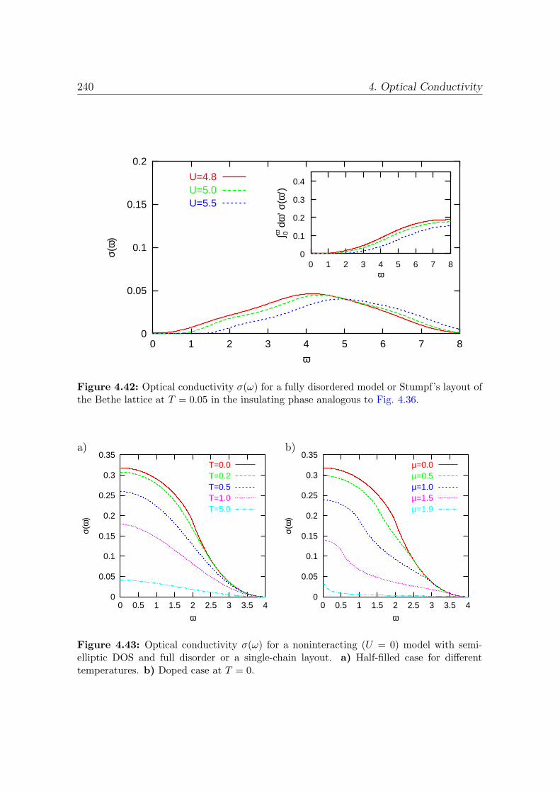
240 4. Optical Conductivity
0
0.05
0.1
0.15
0.2
0 1 2 3 4 5 6 7 8
σ(ω
)
ω
U=4.8U=5.0U=5.5
0
0.1
0.2
0.3
0.4
0 1 2 3 4 5 6 7 8
∫ 0ω d
ω’ σ
(ω’)
ω
Figure 4.42: Optical conductivity σ(ω) for a fully disordered model or Stumpf’s layout ofthe Bethe lattice at T = 0.05 in the insulating phase analogous to Fig. 4.36.
a) b)
0
0.05
0.1
0.15
0.2
0.25
0.3
0.35
0 0.5 1 1.5 2 2.5 3 3.5 4
σ(ω
)
ω
T=0.0T=0.2T=0.5T=1.0T=5.0
0
0.05
0.1
0.15
0.2
0.25
0.3
0.35
0 0.5 1 1.5 2 2.5 3 3.5 4
σ(ω
)
ω
µ=0.0µ=0.5µ=1.0µ=1.5µ=1.9
Figure 4.43: Optical conductivity σ(ω) for a noninteracting (U = 0) model with semi-elliptic DOS and full disorder or a single-chain layout. a) Half-filled case for differenttemperatures. b) Doped case at T = 0.

4.6. QMC Results for the Bethe Lattice 241
a) b)
0
0.1
0.2
0.3
0.4
0.5
4 4.2 4.4 4.6 4.8 5 5.2 5.4 5.6
∫ 0∞ d
ω σ
(ω)
U
f-sum: isotropicf-sum: disordered
f-sum: stacked-π/2 Ekin
0
0.1
0.2
0.3
0.4
0.5
4 4.2 4.4 4.6 4.8 5 5.2 5.4 5.6∫ 0∞
dω
σ(ω
)
U
f-sum: isotropicf-sum: disordered
f-sum: stacked-π/2 Ekin
Figure 4.44: Optical f -sum for models with semi-elliptic DOS, computed by numericalintegration of the results for σ(ω) shown in Fig. 4.34 – Fig. 4.42: a) scaled to unit a andunit variance of the DOS, b) rescaled to unit average hopping distance (division of thef -sum of the isotropic model by 1.05406).
limit U → 0 and T → 0 where only states near the Fermi surface can contributeto transport. Averaged over the whole Brillouin zone, the enhancement is only (ingeneral)
∫∞−∞dε ρ(ε) which equals the average hopping distance
∑∞D=1Dt
∗D
2; using thevalues for the hopping amplitudes given in Table 2.1, it evaluates here to 1.05406.A corresponding increase in the f -sum in the limits T → ∞ and/or U → ∞ can beread off from the form (4.86) of the f -sum rule since in these cases the derivative ofthe momentum distribution function becomes asymptotically constant (as a functionof ε). This asymptotic behavior is already well approached for U = 5.5 as seen inFig. 4.45b. If the asymptotic enhancement is removed by scaling the average hoppingdistance to unity (Fig. 4.44b), the f -sums of the isotropic and of the stacked model(as well as of the disordered model) are nearly identical.
In Fig. 4.46, partial contributions to the f -sum rule are displayed as a functionof momentum ε so that the f -sums shown above would be obtained by integrationover ε. The picture differs considerably depending on whether the sum rule is usedin terms of the momentum distribution function nε as in Fig. 4.46a or in terms of itsderivative as in Fig. 4.46b . In both cases, however, the isotropic model (thick lines)implies contributions to σ(ω) which arise from smaller values of |ε| than the stackedmodel (thin lines). This is true in particular for the metallic phase at U = 4.0;transport is here dominated by states near the Fermi surface. Such behavior isnot only consistent with Fermi-liquid theory, but also most compatible with theDMFT approach: nongeneric momenta with extremal |ε| should not influence resultsof DMFT calculations.

242 4. Optical Conductivity
a) b)
0.1
0.2
0.3
0.4
0.5
0.6
0.7
0.8
0.9
-2 -1.5 -1 -0.5 0 0.5 1 1.5 2
n ε
ε
U=4.0U=4.7U=5.5
0
0.1
0.2
0.3
0.4
0.5
0.6
-2 -1.5 -1 -0.5 0 0.5 1 1.5 2
-dn ε
/dε
ε
U=4.0U=4.7U=5.5
Figure 4.45: a) Momentum distribution function nε as defined in (4.79) and b) (minus)its derivative.
a) b)
-0.2
-0.1
0
0.1
0.2
0.3
0.4
-2 -1.5 -1 -0.5 0 0.5 1 1.5 2
~ ρ’(ε
) n ε
ε
U=4.0U=4.7U=5.5
0
0.1
0.2
0.3
-2 -1.5 -1 -0.5 0 0.5 1 1.5 2
-~ ρ(ε)
dn ε
/dε
ε
U=4.0U=4.7U=5.5
Figure 4.46: Contributions to the f -sum as a function of “momentum” ε for the redefinedBethe lattice (thick lines) and the stacked Bethe lattice (thin lines) corresponding to theequivalent formulations a) (4.86) and b) (4.87) of the f -sum rule.
4.7 Conclusion
In this chapter, we have presented studies of the optical conductivity σ(ω) and itsf -sum rule in high dimensions with particular focus on “the Bethe lattice”, i.e., aclass of lattices with semi-elliptic density of states (DOS).
Initially, the project of computing numerical estimates of σ(ω) on the basis ofquantum Monte Carlo (QMC) solutions of the half-filled Hubbard model with asemi-elliptic DOS seemed straightforward: The formalism had already been worked
4.7. Conclusion 243
out for the hypercubic (hc) lattice and had been applied for general filling basedon NCA (Pruschke et al., 1993) and QMC (Jarrell, Freericks, and Pruschke, 1995)calculations. Rozenberg et al. (1995) had even applied the same formalism to theBethe lattice case (on the basis of ED and IPT data) and extensively discussed thef -sum rule in this context. Indeed, our implementation of the algorithm was soonaccomplished; using an early version of our set of programs, results were publishedfor a manganite model (Held and Vollhardt, 2000). However, we realized that theconventional treatment and the resulting f -sum rule were specific to the hypercubiclattice and not directly applicable to the Bethe lattice. In particular, we foundnumerical violations of the (incorrect) sum rule stated by Rozenberg. In addition,Janis (1999) claimed the foundation of the DMFT treatment of conductivities to beincorrect.53 Thus, we found it necessary to thoroughly check the formalism and toderive extensions for the general case in high dimensions.
We have carefully reviewed the Kubo formalism for the optical conductivity andthe simplifications in the limit of infinite dimensionality (or, more generally, infinitecoordination number). We have presented the first evaluation of the theory in thecase of t−t′ hopping and have shown that Merino and McKenzie’s (2000) (unjustified)use of the conventional hc formalism leads to significant errors in the computationof the transverse conductivity and the thermal conductivity. We have derived a newexpression of the optical f -sum rule which is universally valid within the DMFT andadditionally a form specific to the general dispersion formalism developed in Sec. 2.3.
We have presented a comprehensive discussion of the optical conductivity for lat-tices with semi-elliptic “Bethe” DOS in infinite dimensions. In particular, we havediscovered a flaw in Freericks’s (2000) derivation of σ(ω) for a tree-like layout of theBethe lattice and have shown that the assumption under which Millis (2002) ob-tained essentially the same result is equally unfounded. We have pointed out thatan application of the hc formalism generally implies anisotropic transport and haveestablished the connection between the f -sum and a static local property of suchmodels. We have further demonstrated and explained the incoherence of transportresulting from Stumpf’s (1999) single-chain layout of the Bethe lattice or from strongoffdiagonal disorder and have developed a necessary criterion for coherent transportin the noninteracting limit. We have also presented the first consistent derivation forσ(ω) compatible with a semi-elliptic DOS that implies isotropic transport which isfully coherent in the noninteracting limit. This redefinition of the Bethe lattice (inthe DMFT sense) as an isotropic, regular and clean lattice by the general dispersionmethod and the demonstration that the associated transport properties are robust(with respect to finite dimensionality or hopping range) removes, finally, the patholo-gies previously associated with the DMFT treatment of transport in connection withnon-Gaussian DOSs.
We have written programs for the DMFT computation of conductivities (on thebasis of local spectra) for arbitrary lattice types and have developed a scheme that
53It has become clear later that Janis’s (1999) statement “the current-current correlation functionand consequently the electrical conductivity do have nontrivial vertex corrections in the mean-fieldlimit contrary to what has been up to now assumed from symmetry considerations within the con-serving scheme” does not apply to the optical conductivity (i.e., in the long-wavelength limit).
244 4. Optical Conductivity
is particularly robust in combination with the QMC code and the variant of themaximum entropy method used within this work. The high accuracy of our methodhas been successfully tested by comparison with a newly established sum rule for the(real-frequency) self-energy. We have presented numerical results for σ(ω) of the half-filled Hubbard model with semi-elliptic DOS near the metal-insulator transition forall valid definitions, i.e., for the incoherent models, the anisotropic stacked model, andfor the new isotropic “redefined Bethe lattice”. Comparing the qualitative features,the Drude weight, and the f -sums, we have shown that the exact definition doesmatter in general, in particular for not too large interaction.
We have pointed out in the beginning of this chapter that f -sum rules as discussedabove may be regarded as artifacts of the single-band assumption. While they maystill be useful as approximate partial sum rules, a different, universal f -sum rule isobtained in a full model. We have only briefly touched upon additional features inσ(ω) which are specific to multi-band models or to non-Bravais lattices. Furthermorewe had to limit the discussion of finite dimensionality to a fully local theory wherethe bubble formula for σ(ω) remains valid; vertex corrections not included in thisapproximation are expected to increase the static conductivity since the importanceof umklapp scattering is reduced (Uhrig and Vollhardt, 1995). On the other hand,a reduction of the static conductivity and a broadening of the Drude peak is ex-pected to result from impurities and from electron-phonon interaction, which werealso neglected in this chapter.

245
Chapter 5
Realistic Modeling of StronglyCorrelated Materials
Well-controlled studies of abstract models like the one-band Hubbard model as pre-sented in the preceding chapters shed light on important physical phenomena, evenwhen the models themselves are neither fully realistic nor complete (full frustration,single-band assumption, etc.). Still, one ultimate goal of condensed matter theory isa controlled description of materials which is as realistic as possible and allows for amaterial-specific calculation of a wide range of properties. One step into this direc-tion, although not fully controlled, is the recently developed LDA+DMFT methodwhich we will apply in this chapter for modeling the doped transition metal oxideLa1-xSrxTiO3. We will introduce the material under investigation and demonstratethe failure of LDA to reproduce its photoemission spectrum in Sec. 5.1, then discussconventional density functional theory in Sec. 5.2 and introduce the LDA+DMFTmethod in Sec. 5.3. Numerical results will be presented and compared with experi-ments in Sec. 5.4.
The work presented in this chapter was started in a collaboration with the Opticsof Metals Laboratory at the Institute of Metal Physics of the Ural Division of theRussian Academy of Sciences in Yekaterinburg lead by Prof. V. I. Anisimov. Inparticular, all LDA calculations were performed by Igor Nekrasov from Anisimov’sgroup. The initial QMC and MEM results presented in subsection 5.4.1 were mainlycalculated by Nekrasov and Held using Held’s multi-band version of the QMC codewhile the photoemission spectra were obtained using an analysis program written aspart of this thesis. The QMC computations at higher accuracy and the study of theimpact of different MEM procedures on the resulting spectra presented in subsection5.4.2 as well as the calculation of transport properties in subsection 5.4.3 were alsoperformed by the author of this thesis.

246 5. Realistic Modeling of Strongly Correlated Materials
• Ti
• La, Sr
• O
α
Ti 3de
t2g
g
a) b)
c)
Figure 5.1: Structure of La1-xSrxTiO3 : a) Idealized (cubic) perovskite structure: Ti ionsare octahedrally coordinated by oxygen in a cubic matrix of sites occupied by either La orSr (presumably disordered). The size of spheres in the figure is not related to ionic radii.b) Orthorhombic distortion, i.e., alternating tilting of oxygen octahedra which reduces theangle Ti-O-Ti to α ≈ 155. c) Scheme of band degeneracy; the t2g band contains oneelectron per unit cell for LaTiO3 and is empty for SrTiO3.
5.1 La1-xSrxTiO3, a Strongly Correlated Transition
Metal Oxide
La1-xSrxTiO3 belongs to a large class of 3d transition metal oxides of compositionABO3, where A is a rare earth or alkalide (or a nonstoichiometric combinationthereof) and B a transition metal and which crystallize in the orthorhombically dis-torted perovskite (GdFeO3-type) structure. The idealized cubic perovskite structureis shown in Fig. 5.1a. In the distorted perovskite, the almost perfectly rigid oxygenoctahedra tilt alternatingly in all space directions so that the angle α (Ti-O-Ti) isreduced from its cubic value of 180 to, e.g., α ≈ 155 for La1-xSrxTiO3 (MacLean,Ng, and Greedan, 1979), see Fig. 5.1b.1 Formally, pure SrTiO3 is an ionic insulatorwhere all ions reach noble gas configurations.2 In fact, this material is a band insu-lator which is seen both in experiment and band structure calculations and makesthis material well-suited as substrate or spacer material for high-Tc superconductingfilms.3 Both experiment and band-structure calculations imply that La donates 3
1The degree of distortion can in general be estimated from ionic radii in terms of the tolerancefactor f = (rA + rO)/(
√2(rB + rO)), where f ≈ 0.8 corresponds to α ≈ 140 and f ≈ 0.95
corresponds to α ≈ 157, respectively (Imada et al., 1998).2O needs 2 electrons to obtain the [Ne] configuration; the atomic configuration is [Kr] 5s2 for Sr,
[Ar] 3d14s2 for Ti, and [Xe] 5d16s2 for La.3The chemically reduced component, SrTiO3−δ, is a superconductor with Tc . 0.5 K (Schooley,
Hosler, Ambler, Becker, Cohen, and Koonce, 1965).
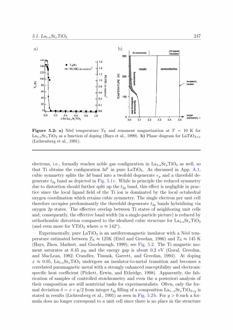
5.1. La1-xSrxTiO3 247
a) b)
Figure 5.2: a) Neel temperature TN and remanent magnetization at T = 10 K forLa1-xSrxTiO3 as a function of doping (Hays et al., 1999). b) Phase diagram for LaTiO3+x
(Lichtenberg et al., 1991).
electrons, i.e., formally reaches noble gas configuration in La1-xSrxTiO3 as well, sothat Ti obtains the configuration 3d1 in pure LaTiO3. As discussed in App. A.1,cubic symmetry splits the 3d band into a twofold degenerate eg and a threefold de-generate t2g band as depicted in Fig. 5.1c. While in principle the reduced symmetrydue to distortion should further split up the t2g band, this effect is negligible in prac-tice since the local ligand field of the Ti ion is dominated by the local octahedraloxygen coordination which retains cubic symmetry. The single electron per unit celltherefore occupies predominantly the threefold degenerate t2g bands hybridizing viaoxygen 2p states. The effective overlap between Ti states of neighboring unit cellsand, consequently, the effective band width (in a single-particle picture) is reduced byorthorhombic distortion compared to the idealized cubic structure for La1-xSrxTiO3
(and even more for YTiO3 where α ≈ 142).
Experimentally, pure LaTiO3 is an antiferromagnetic insulator with a Neel tem-perature estimated between TN ≈ 125K (Eitel and Greedan, 1986) and TN ≈ 145 K(Hays, Zhou, Markert, and Goodenough, 1999); see Fig. 5.2. The Ti magnetic mo-ment saturates at 0.45 µB and the energy gap is about 0.2 eV (Goral, Greedan,and MacLean, 1982; Crandles, Timusk, Garrett, and Greedan, 1994). At dopingx ≈ 0.05, La1-xSrxTiO3 undergoes an insulator-to-metal transition and becomes acorrelated paramagnetic metal with a strongly enhanced susceptibility and electronicspecific heat coefficient (Pickett, Erwin, and Ethridge, 1998). Apparently, the fab-rication of samples of controlled stoichiometry and even the a posteriori analysis oftheir composition are still nontrivial tasks for experimentalists. Often, only the for-mal deviation δ = x+ y/2 from integer t2g filling of a composition La1−xSrxTiO3+y isstated in results (Lichtenberg et al., 1991) as seen in Fig. 5.2b. For y > 0 such a for-mula does no longer correspond to a unit cell since there is no place in the structure
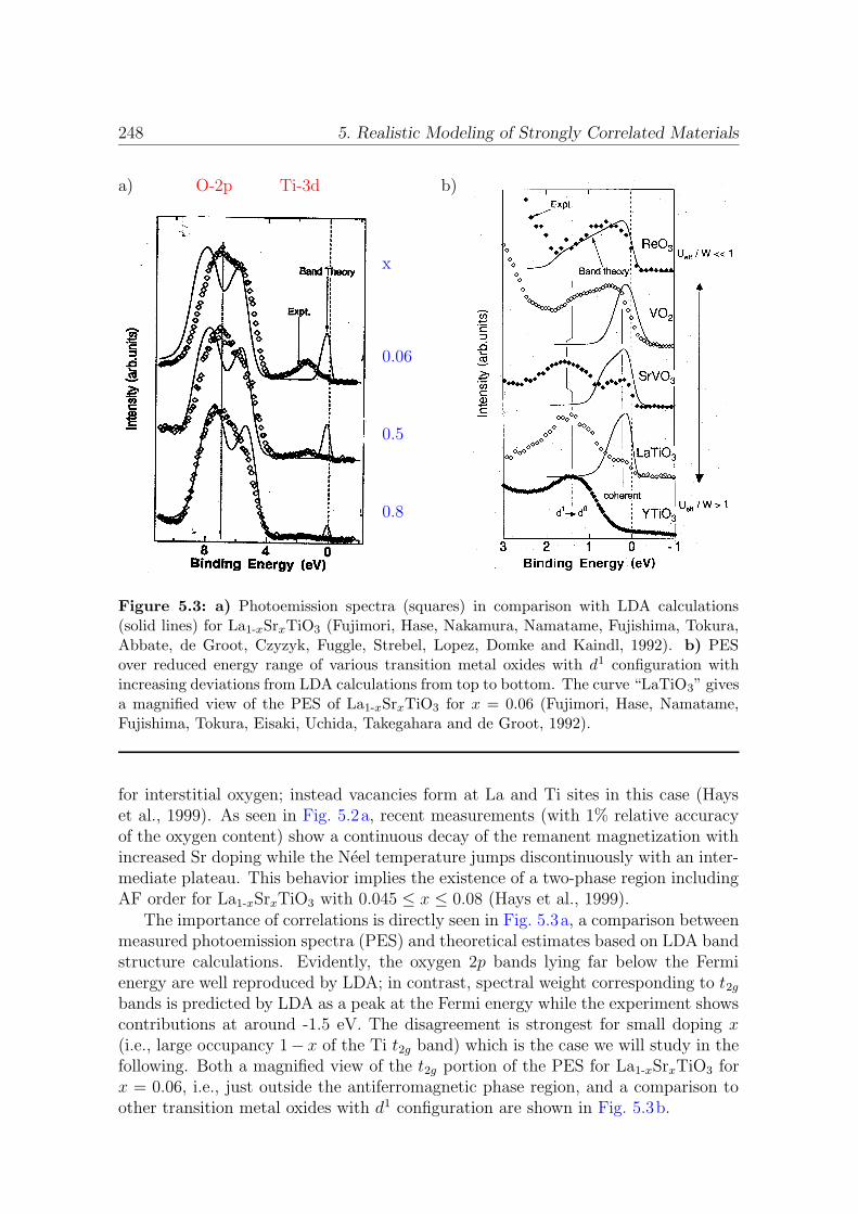
248 5. Realistic Modeling of Strongly Correlated Materials
O-2p Ti-3d
x
0.06
0.5
0.8
a) b)
Figure 5.3: a) Photoemission spectra (squares) in comparison with LDA calculations(solid lines) for La1-xSrxTiO3 (Fujimori, Hase, Nakamura, Namatame, Fujishima, Tokura,Abbate, de Groot, Czyzyk, Fuggle, Strebel, Lopez, Domke and Kaindl, 1992). b) PESover reduced energy range of various transition metal oxides with d1 configuration withincreasing deviations from LDA calculations from top to bottom. The curve “LaTiO3” givesa magnified view of the PES of La1-xSrxTiO3 for x = 0.06 (Fujimori, Hase, Namatame,Fujishima, Tokura, Eisaki, Uchida, Takegahara and de Groot, 1992).
for interstitial oxygen; instead vacancies form at La and Ti sites in this case (Hayset al., 1999). As seen in Fig. 5.2a, recent measurements (with 1% relative accuracyof the oxygen content) show a continuous decay of the remanent magnetization withincreased Sr doping while the Neel temperature jumps discontinuously with an inter-mediate plateau. This behavior implies the existence of a two-phase region includingAF order for La1-xSrxTiO3 with 0.045 ≤ x ≤ 0.08 (Hays et al., 1999).
The importance of correlations is directly seen in Fig. 5.3a, a comparison betweenmeasured photoemission spectra (PES) and theoretical estimates based on LDA bandstructure calculations. Evidently, the oxygen 2p bands lying far below the Fermienergy are well reproduced by LDA; in contrast, spectral weight corresponding to t2gbands is predicted by LDA as a peak at the Fermi energy while the experiment showscontributions at around -1.5 eV. The disagreement is strongest for small doping x(i.e., large occupancy 1− x of the Ti t2g band) which is the case we will study in thefollowing. Both a magnified view of the t2g portion of the PES for La1-xSrxTiO3 forx = 0.06, i.e., just outside the antiferromagnetic phase region, and a comparison toother transition metal oxides with d1 configuration are shown in Fig. 5.3b.
5.2. DFT and LSDA 249
5.2 Density Functional Theory and Local Spin
Density Approximation
Density functional theory (DFT) is, originally, an approach for calculating groundstate properties via a mapping of the full interacting many-body problem onto aneffective single-particle problem. It is based on the observation that the ground stateenergy of any N -electron system can be written as a functional of the electronicdensity ρ(r) alone (Hohenberg and Kohn, 1964). Following Levy’s (1979) proof,we split up the full electronic Hamiltonian (1.2) into internal contributions T + Veeand the external contribution Vext with 〈Vext〉 =
∫drVext(r)ρ(r) =: Eext[ρ] . Since
both the kinetic energy T and the Coulomb electron-electron interaction Vee have auniversal form, the functional
F [ρ] := minψ
〈ψ|T + Vee|ψ〉∣∣∣ 〈ψ|ρ(r)|ψ〉 = ρ(r)
, (5.1)
where ρ(r) measures the density at site r and ψ denotes a fermion many-body wavefunction, is indeed universal,4 i.e., a functional of the density alone. In terms of thisfunctional, the basic theorems of DFT read
E[ρ] := F [ρ] +
∫
dr Vext ρ(r) ≥ EGS , (5.2)
F [ρGS] +
∫
dr Vext ρGS(r) = EGS , (5.3)
i.e., the energy functional E[ρ] defined in (5.2) is both an upper bound to the trueground state energy EGS for arbitrary density distribution and coincides with EGS
for the true ground state density distribution ρGS.5 The first theorem (5.2) follows
from an application of the usual variational principle 〈ψ|T + Vee + Vext|ψ〉 ≥ EGS tothe wave function ψmin which minimizes the r.h.s. expression in (5.1). On the otherhand, each ground state wave function ψGS also minimizes T + Vee in (5.1) for fixedground state density which proves (5.3). If the universal functional F [ρ] was knownexplicitly and could be evaluated efficiently the ground state energy could be obtainedin an arbitrary external potential by minimizing E[ρ] defined in (5.2). Other groundstate properties could then be obtained using corresponding (possibly multi-valued)functionals. In practice, however, a controlled computation of F [ρ] along the lines of(5.1) (which would require the solution of jellium models with constrained density)is not possible.
In this situation, it is useful to split up the energy functional differently (Kohnand Sham, 1965),
E[ρ] = T0[ρ] + Eext[ρ] + EHartree[ρ] + Exc[ρ], (5.4)
4Note that the proof reproduced here implies universality of the functional F [ρ] only for fixedparticle number N . Implicitly, one usually assumes that the thermodynamic limit of the formalismis well defined.
5One can show that even the external potential is a functional of the ground state density(Hohenberg and Kohn, 1964). This finding is, however, not used in actual calculations and does notextend to spin-resolved DFT with inclusion of magnetic fields (Capelle and Vignale, 2001).

250 5. Realistic Modeling of Strongly Correlated Materials
where T0[ρ] is not the true kinetic energy (Jones and Gunnarsson, 1989), but thekinetic energy of a noninteracting N -particle system with density distribution ρ(r);Eext was defined above and the Hartree energy is given by
EHartree =1
2
∫
dr dr′ Vee(r − r′)ρ(r)ρ(r′) . (5.5)
The first three terms in (5.4) can be treated exactly, so that the methodologicalproblem is reduced to finding a good approximation for the exchange-correlationenergy for which (5.4) is a defining equation in connection with (5.1), (5.2), and(5.5). This energy functional can be assumed to be much less dependent on detailsof the density distribution than the full functional which includes very large kineticenergy terms. Given an (approximate) explicit expression for Exc[ρ], the ground stateproperties EGS and ρGS of some specified system are then found numerically by aself-consistent solution of the Kohn-Sham equations,
[
− ~2
2me
∇+ Vext(r) +
∫
dr′ρ(r′)Vee(r − r′) +δExc[ρ]
δρ(r)
]
ϕi(r) = εi ϕi(r) , (5.6)
i.e., a Schrodinger-like equation for a set of single-particle wave functions ϕiNi=1
which reproduce the density ρ(r) =∑N
i=1 |ϕi(r)|2. Note that these wave functionsand the associated eigenvalues εi have no direct meaning in the context of the originalmany-body problem.
In the DFT calculations presented in this work we follow the usual approach oftreating the functional Exc in local spin density approximation (LDA or LSDA),6
Exc[ρ] ≈∫
dr ρ(r) vLDAxc
(ρ↑(r), ρ↓(r)
), (5.7)
where the functional dependence of vLDAxc is usually taken from parameterizations of
solutions of simplified jellium models (von Barth and Hedin, 1972; Gunnarsson andLundqvist, 1976) or from the QMC solution by Ceperley and Alder (1980) of the jel-lium model (Vosko and Wilk, 1980; Perdew and Zunger, 1981). Different parameter-izations lead to slightly different results, but are all free from adjustable parameters.For exact properties of Exc[ρ] and possible general approximations beyond LDA see,e.g., the review by Jones and Gunnarsson (1989).
Even though the LDA problem (5.6) with (5.7) is conceptually much simpler thanthe original many-body problem, its numerically stable solution in the presence ofsingular ion potentials and for a relatively large number of electrons is still a non-trivial task. For condensed matter problems7 one may distinguish full-potential from
6It is easy to check that the above derivations directly generalize to functionals F [ρ↑, ρ↓] andE[ρ↑, ρ↓] of the spin density. While in principle the approaches with and without explicit spinresolution are equivalent (cf. footnote 5 on page 249) since ρ↑ and ρ↓ are functionals of ρ, itis found that better approximations to the exchange-correlation energy are available in terms of thespin resolved densities.
7Specialized methods and, in particular, basis sets for the single-particle wave functions ϕi existfor quantum chemistry problems.

5.3. LDA+DMFT 251
pseudopotential approaches where the latter use weak effective potentials for valenceelectrons in order to get rid of core oscillations which would require very large basissets in plane-wave expansions. While newer codes allow for efficient full-potential cal-culations in a linear augmented plane wave (LAPW) basis [as, e.g., Blaha, Schwarz,and Luitz’s (1999) package VIENNA], the problem can be avoided by using atomic-like basis sets at least near the ionic cores. In the muffin-tin orbital (MTO) approach,a minimal basis characterized by angular momentum quantum numbers is constructedwhere the external potential only acts inside a spherical “muffin tin”. The energydependence of the MTOs is linearized and an energy-independent set obtained in theLMTO method which is then reliable only for valence states (Andersen, 1975). Liftingthe constraint of minimalism, more localized8 “tight binding” basis functions wereintroduced in the TB-LMTO approach (Andersen, Pawlowska, and Jepsen, 1986)which is usually used in connection with the atomic sphere approximation (ASA) ofa locally spherical resulting potential.
It should be stressed that DFT as a ground state method cannot directly be usedfor the determination of excitation spectra. In principle, apart from true ground stateproperties, only the sizes of energy gaps can be computed as differences of groundstate energies for systems with N and N + 1 electrons, respectively. In practice,however, the eigenvalues εi of the single particle problem (5.6) often compare favor-ably with experiment and are regularly regarded as band structures of the interactingsystem.
The various LDA methods have been used successfully for the computation of bulkproperties of materials, in particular metals, as well as surface or impurity effects.While their superiority over preceding DFTs such as the Thomas-Fermi approxima-tion can be explained from the vastly improved treatment of the kinetic energy, theaccuracy of LDA, an effective single-particle theory without adjustable parameters(“ab initio”) came as a surprise not only to its inventors. Still, LDA fails for impor-tant classes of materials with strong electronic correlations like La1-xSrxTiO3, whichlimits its general predictive power. In the next section we will discuss extensions ofthe LDA approach which address this problem.
5.3 LDA+DMFT
Since the LDA uses input from the jellium model, it is not surprising that the resultingerrors are larger for localized than for extended states. One may suspect that bothlocal correlations and the self-interaction contribute significantly to these errors forlocalized orbitals. In fact, self-interaction corrected (SIC-LDA) calculations yield amuch better estimate for the total energy of isolated atoms than plain LDA which canbe attributed to an improved treatment of core states.9 Using a basis with localized
8Conventional MTOs fall off as r−(l+1) for angular momentum l.9For the total energy of, e.g., Ne atoms, LDA is even inferior to the Hartree-Fock theory (HF).
For ionization energies, however, the agreement with experiment is significantly better for LSDAthan either for LDA or HF with no general improvement from inclusion of SIC (Gunnarsson andJones, 1981).
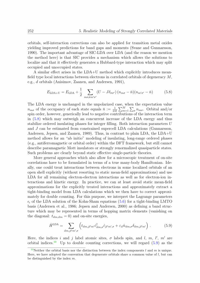
252 5. Realistic Modeling of Strongly Correlated Materials
orbitals, self-interaction corrections can also be applied for transition metal oxidesyielding improved predictions for band gaps and moments (Svane and Gunnarsson,1990). The important advantage of SIC-LDA over LDA (and the reason we mentionthe method here) is that SIC provides a mechanism which allows the solutions tolocalize and that it effectively generates a Hubbard-type interaction which may splitoccupied and unoccupied states.
A similar effect arises in the LDA+U method which explicitly introduces mean-field type local interactions between electrons in correlated orbitals of degeneracy M ,e.g., d orbitals (Anisimov, Zaanen, and Andersen, 1991),
ELDA+U = ELDA +1
2
∑
mσ 6=m′σ′
(U − Jδσσ′) (nmσ − n)(nm′σ′ − n) (5.8)
The LDA energy is unchanged in the unpolarized case, when the expectation valuenmσ of the occupancy of each state equals n := 1
2M
∑Mm=1
∑
σ nmσ. Orbital and/orspin order, however, generically lead to negative contributions of the interaction termin (5.8) which may outweigh an concurrent increase of the LDA energy and thusstabilize ordered insulating phases for integer filling. Both interaction parameters Uand J can be estimated from constrained supercell LDA calculations (Gunnarsson,Andersen, Jepsen, and Zaanen, 1989). Thus, in contrast to plain LDA, the LDA+Umethod allows for an “ab initio” modeling of insulating, long-range ordered phases(e.g., antiferromagnetic or orbital order) within the DFT framework, but still cannotdescribe paramagnetic Mott insulators or strongly renormalized quasiparticle states.Such problems are clearly beyond static effective single-particle theories.
More general approaches which also allow for a microscopic treatment of on-sitecorrelations have to be formulated in terms of a true many-body Hamiltonian. Ide-ally, one could treat interactions between electrons in some localized orbitals of anopen shell explicitly (without resorting to static mean-field approximations) and useLDA for all remaining electron-electron interactions as well as for electron-ion in-teractions and kinetic energy. In practice, we can at least avoid static mean-fieldapproximations for the explicitly treated interactions and approximately extract atight-binding model from LDA calculations which we then have to correct approxi-mately for double counting. For this purpose, we interpret the Lagrange parametersεi of the LDA solution of the Kohn-Sham equations (5.6) for a tight-binding LMTObasis (Andersen et al., 1986; Jepsen and Andersen, 2000) as defining a band struc-ture which may be represented in terms of hopping matrix elements (vanishing onthe diagonal: tilm,ilm = 0) and on-site energies,
HLDA =∑
ilm,jl′m′,σ
(
tilm,jl′m′ c†ilm,σ cjl′m′,σ + εilnilm,σδilm,jl′m′
)
. (5.9)
Here, the indices i and j label atomic sites, σ labels spin, and l, m, l′, m′ areorbital indices.10 Up to double counting corrections, we will regard (5.9) as the
10Neither the orbital basis nor the distinction between the index components l and m is unique.Here, we have adopted the convention that degenerate orbitals share a common value of l, but canbe distinguished by the index m.
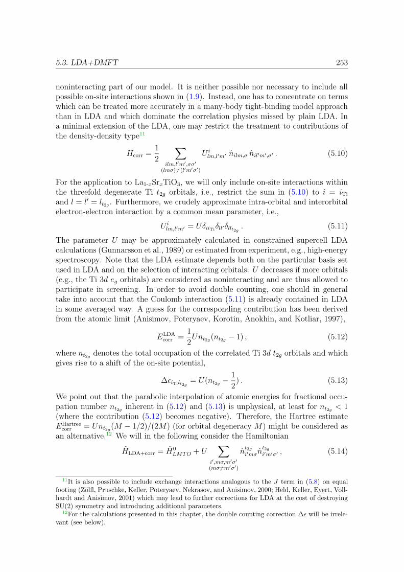
5.3. LDA+DMFT 253
noninteracting part of our model. It is neither possible nor necessary to include allpossible on-site interactions shown in (1.9). Instead, one has to concentrate on termswhich can be treated more accurately in a many-body tight-binding model approachthan in LDA and which dominate the correlation physics missed by plain LDA. Ina minimal extension of the LDA, one may restrict the treatment to contributions ofthe density-density type11
Hcorr =1
2
∑
ilm,l′m′,σσ′
(lmσ)6=(l′m′σ′)
U ilm,l′m′ nilm,σ nil′m′,σ′ . (5.10)
For the application to La1-xSrxTiO3, we will only include on-site interactions withinthe threefold degenerate Ti t2g orbitals, i.e., restrict the sum in (5.10) to i = iTi
and l = l′ = lt2g. Furthermore, we crudely approximate intra-orbital and interorbital
electron-electron interaction by a common mean parameter, i.e.,
U ilm,l′m′ = UδiiTi
δll′δllt2g. (5.11)
The parameter U may be approximately calculated in constrained supercell LDAcalculations (Gunnarsson et al., 1989) or estimated from experiment, e.g., high-energyspectroscopy. Note that the LDA estimate depends both on the particular basis setused in LDA and on the selection of interacting orbitals: U decreases if more orbitals(e.g., the Ti 3d eg orbitals) are considered as noninteracting and are thus allowed toparticipate in screening. In order to avoid double counting, one should in generaltake into account that the Coulomb interaction (5.11) is already contained in LDAin some averaged way. A guess for the corresponding contribution has been derivedfrom the atomic limit (Anisimov, Poteryaev, Korotin, Anokhin, and Kotliar, 1997),
ELDAcorr =
1
2Unt2g
(nt2g− 1) , (5.12)
where nt2gdenotes the total occupation of the correlated Ti 3d t2g orbitals and which
gives rise to a shift of the on-site potential,
∆εiTilt2g= U(nt2g
− 1
2) . (5.13)
We point out that the parabolic interpolation of atomic energies for fractional occu-pation number nt2g
inherent in (5.12) and (5.13) is unphysical, at least for nt2g< 1
(where the contribution (5.12) becomes negative). Therefore, the Hartree estimateEHartree
corr = Unt2g(M − 1/2)/(2M) (for orbital degeneracy M) might be considered as
an alternative.12 We will in the following consider the Hamiltonian
HLDA+corr = H0LMTO + U
∑
i′,mσ,m′σ′
(mσ 6=m′σ′)
nt2g
i′mσnt2g
i′m′σ′ , (5.14)
11It is also possible to include exchange interactions analogous to the J term in (5.8) on equalfooting (Zolfl, Pruschke, Keller, Poteryaev, Nekrasov, and Anisimov, 2000; Held, Keller, Eyert, Voll-hardt and Anisimov, 2001) which may lead to further corrections for LDA at the cost of destroyingSU(2) symmetry and introducing additional parameters.
12For the calculations presented in this chapter, the double counting correction ∆ε will be irrele-vant (see below).

254 5. Realistic Modeling of Strongly Correlated Materials
where i′ only sums over Ti sites and the double-counting corrected LDA Hamiltonianis assumed as
H0LDA = HLMTO − U(nt2g
− 1
2)∑
i′,mσ
nt2g
i′mσ . (5.15)
In lack of exact methods for the solution of the general multi-band Hubbard model,approximative solutions are needed just like for pure model calculations. A treatmentwithin the DMFT seems natural and appropriate since it treats the local dynamicsinduced by the additional local interactions exactly and was also the first choice his-torically (Anisimov et al., 1997). Lichtenstein and Katsnelson (1998) used DMFT, thefluctuation-exchange approximation (FLEX), and the Hubbard-I approximation al-ternatively and named the general approach LDA++. Drchal, Janis, and Kudrnovsky(1999) combined FLEX with the coherent potential approximation (CPA) for theinclusion of disorder effects.
The DMFT solution of (5.14) is best formulated in reciprocal space, where H0LDA
has the matrix elements(H0
LDA(k))
qlm,q′l′m′=(HLDA(k)
)
qlm,q′l′m′− δqlm,q′l′m′δql,qTilt2g
U(nt2g− 1
2) . (5.16)
Here, q is an index of the atoms in the elementary unit cell. Generalizing from the1-band Bravais lattice case discussed in subsection 1.2.3, the lattice problem can bemapped to a multi-band SIAM.13 Now, on-site lattice Green function G, impurityGreen function G, and self-energy Σ are matrices where each index denotes an orbitalwithin the unit cell, α ≡ (q, l,m). The k integrated lattice Dyson equation and theimpurity Dyson equation read for (complex) frequency z:
Gσαα′(z) =
∫dk
VB
[
zδα,α′ −(H0
LDA(k))
αα′− Σσ
αα′(z)]−1
(5.17)
[Gσαα′(z)
]−1=
[Gσαα′(z)
]−1 − Σσαα′(z) , (5.18)
where [. . . ]−1 denotes matrix inversion (in α, α′). The impurity (or cluster) problem,expressed in mixed notation using imaginary time τ and index n for Matsubarafrequency iωn takes the form:
Gσnαα′ = − 1
Z
∫
D[ψ]D[ψ∗] ψσnα ψσn∗α′ eA[ψ,ψ∗,G] , (5.19)
with the action
A[ψ, ψ∗,G] =∑
n,σ,α,α′
ψσn∗α
[Gσnαα′
]−1ψσnα′
− U
2
∑
m,σ,m′,σ′
(mσ)6=(m′σ′)
β∫
0
dτ ψσn∗
qTilt2gm ψ
σnqTilt2g
m ψσ′n∗qTilt2g
m′ ψσ′n
qTilt2gm′ . (5.20)
13In general, the resulting problem appears rather as a finite cluster with on-site interactions andfrequency dependent on-site “energies” and “hopping terms” very similar to the systems studiedin DCA (cf. App. A.3). Only in absence of hybridization between different orbitals the DMFTmapping leads to a conventional multi-band impurity without mixing terms. Since we will neglectsmall hybridization terms found in the LDA calculations for La1-xSrxTiO3 , however, the clusterwill indeed reduce to a single impurity in our calculations.
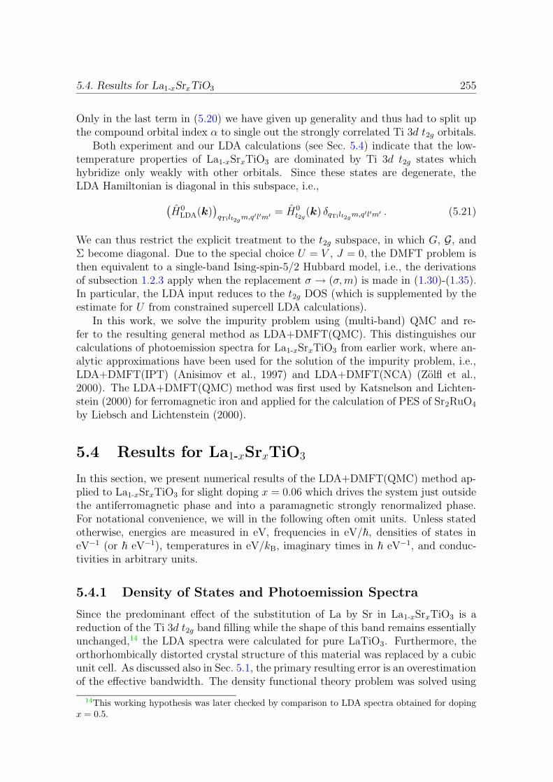
5.4. Results for La1-xSrxTiO3 255
Only in the last term in (5.20) we have given up generality and thus had to split upthe compound orbital index α to single out the strongly correlated Ti 3d t2g orbitals.
Both experiment and our LDA calculations (see Sec. 5.4) indicate that the low-temperature properties of La1-xSrxTiO3 are dominated by Ti 3d t2g states whichhybridize only weakly with other orbitals. Since these states are degenerate, theLDA Hamiltonian is diagonal in this subspace, i.e.,
(H0
LDA(k))
qTilt2gm,q′l′m′
= H0t2g
(k) δqTilt2gm,q′l′m′ . (5.21)
We can thus restrict the explicit treatment to the t2g subspace, in which G, G, andΣ become diagonal. Due to the special choice U = V , J = 0, the DMFT problem isthen equivalent to a single-band Ising-spin-5/2 Hubbard model, i.e., the derivationsof subsection 1.2.3 apply when the replacement σ → (σ,m) is made in (1.30)-(1.35).In particular, the LDA input reduces to the t2g DOS (which is supplemented by theestimate for U from constrained supercell LDA calculations).
In this work, we solve the impurity problem using (multi-band) QMC and re-fer to the resulting general method as LDA+DMFT(QMC). This distinguishes ourcalculations of photoemission spectra for La1-xSrxTiO3 from earlier work, where an-alytic approximations have been used for the solution of the impurity problem, i.e.,LDA+DMFT(IPT) (Anisimov et al., 1997) and LDA+DMFT(NCA) (Zolfl et al.,2000). The LDA+DMFT(QMC) method was first used by Katsnelson and Lichten-stein (2000) for ferromagnetic iron and applied for the calculation of PES of Sr2RuO4
by Liebsch and Lichtenstein (2000).
5.4 Results for La1-xSrxTiO3
In this section, we present numerical results of the LDA+DMFT(QMC) method ap-plied to La1-xSrxTiO3 for slight doping x = 0.06 which drives the system just outsidethe antiferromagnetic phase and into a paramagnetic strongly renormalized phase.For notational convenience, we will in the following often omit units. Unless statedotherwise, energies are measured in eV, frequencies in eV/~, densities of states ineV−1 (or ~ eV−1), temperatures in eV/kB, imaginary times in ~ eV−1, and conduc-tivities in arbitrary units.
5.4.1 Density of States and Photoemission Spectra
Since the predominant effect of the substitution of La by Sr in La1-xSrxTiO3 is areduction of the Ti 3d t2g band filling while the shape of this band remains essentiallyunchanged,14 the LDA spectra were calculated for pure LaTiO3. Furthermore, theorthorhombically distorted crystal structure of this material was replaced by a cubicunit cell. As discussed also in Sec. 5.1, the primary resulting error is an overestimationof the effective bandwidth. The density functional theory problem was solved using
14This working hypothesis was later checked by comparison to LDA spectra obtained for dopingx = 0.5.
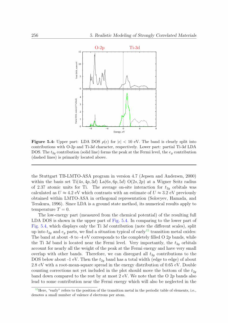
256 5. Realistic Modeling of Strongly Correlated Materials
O-2p Ti-3d
−8 −4 0 4 8Energy, eV
0
1
2
3
4
Part
ial D
OS,
sta
tes/
(eV
*orb
ital)
0
5
10
15
Tot
al D
OS,
sta
tes/
eV
Figure 5.4: Upper part: LDA DOS ρ(ε) for |ε| < 10 eV. The band is clearly split intocontributions with O-2p and Ti-3d character, respectively. Lower part: partial Ti-3d LDADOS. The t2g contribution (solid line) forms the peak at the Fermi level, the eg contribution(dashed lines) is primarily located above.
the Stuttgart TB-LMTO-ASA program in version 4.7 (Jepsen and Andersen, 2000)within the basis set Ti(4s, 4p, 3d) La(6s, 6p, 5d) O(2s, 2p) at a Wigner Seitz radiusof 2.37 atomic units for Ti. The average on-site interaction for t2g orbitals wascalculated as U ≈ 4.2 eV which contrasts with an estimate of U ≈ 3.2 eV previouslyobtained within LMTO-ASA in orthogonal representation (Solovyev, Hamada, andTerakura, 1996). Since LDA is a ground state method, its numerical results apply totemperature T = 0.
The low-energy part (measured from the chemical potential) of the resulting fullLDA DOS is shown in the upper part of Fig. 5.4. In comparing to the lower part ofFig. 5.4, which displays only the Ti 3d contribution (note the different scales), splitup into t2g and eg parts, we find a situation typical of early15 transition metal oxides:The band at about -8 to -4 eV corresponds to the completely filled O 2p bands, whilethe Ti 3d band is located near the Fermi level. Very importantly, the t2g orbitalsaccount for nearly all the weight of the peak at the Fermi energy and have very smalloverlap with other bands. Therefore, we can disregard all t2g contributions to theDOS below about -1 eV. Then the t2g band has a total width (edge to edge) of about2.8 eV with a root-mean-square spread in the energy distribution of 0.65 eV. Doublecounting corrections not yet included in the plot should move the bottom of the t2gband down compared to the rest by at most 2 eV. We note that the O 2p bands alsolead to some contribution near the Fermi energy which will also be neglected in the
15Here, “early” refers to the position of the transition metal in the periodic table of elements, i.e.,denotes a small number of valence d electrons per atom.

5.4. Results for La1-xSrxTiO3 257
a) b)
0
0.2
0.4
0.6
0.8
1
-4 -2 0 2 4 6
A(ω
)
ω
QMC: U=3.2LDA (U=0)
0
0.1
0.2
0.3
0.4
0.5
-4 -2 0 2 4 6A
(ω)
ω
U=3.2U=4.0
U=4.25U=5.0
0.1
0.2
0.3
-0.2 0 0.2
LDA
Figure 5.5: a) Partial Ti 3d t2g LDA+DMFT(QMC) DOS for T = 0.1 eV and U = 3.2eV in comparison to LDA. b) Partial Ti 3d t2g LDA+DMFT(QMC) DOS for T = 0.1 fordifferent interaction strengths. Inset: magnified view for small energies (including LDA).
following except when we discuss inverse photoemission (see Fig. 5.14).For the solution of (5.14) for La1-xSrxTiO3 (x = 0.06) within the DMFT, the self-
consistency equations were iterated to convergence using QMC at a relatively hightemperature kBT = 0.1 eV, i.e., T ≈ 1160 K and with a discretization ∆τ = 0.25eV−1.Here, the filling was fixed to 1−x by adjusting the chemical potential (set to 0 in theresulting spectra). Then, 40 measurements for the imaginary-time Green functionG(τi) on the discretized grid were performed with fixed self-energy. Finally, real-timepartial t2g spectra were obtained using Sandvik’s MEM program. As seen in Fig. 5.5a,the explicit inclusion of a finite on-site interaction U = 3.2 eV changes the shape ofthe spectrum near the Fermi energy dramatically: in addition to the quasiparticlepeak, a remnant of the noninteracting LDA DOS, lower and upper Hubbard bandsappear. The spectral density A(ω) right at the Fermi energy is almost pinned toits noninteracting value, even at this comparatively high temperature. The result ofcorresponding calculations is shown in Fig. 5.5b also for U = 4 eV, U = 4.25 eV,and U = 5.0 eV. The spread of interaction values 3.2 eV . U . 5.0 eV reflects theintrinsic uncertainty in the LDA estimate for U . Clearly, the quasiparticle weightdecreases with increasing U . The relatively large difference between the spectraobtained for U = 4.0 and U = 4.25 indicates significant intrinsic uncertainties whichwe will discuss in subsection 5.4.2.
We compare our QMC result for U = 4.0 with approximate solutions of theDMFT problem in Fig. 5.6 at the same temperature T = 0.1 eV, i.e., T ≈ 1160 K.Most prominently, IPT misses the quasiparticle peak at this temperature since thisapproximation underestimates the associated Kondo temperature [cf. related obser-vations for a three-band Hubbard model with Bethe DOS by Kajueter and Kotliar(1997)]. Moreover, the tails of the IPT spectral functions appear to have too much
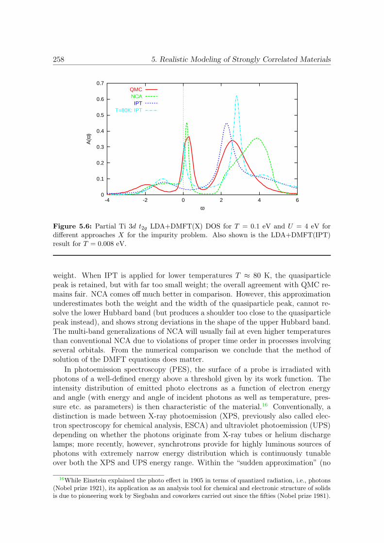
258 5. Realistic Modeling of Strongly Correlated Materials
0
0.1
0.2
0.3
0.4
0.5
0.6
0.7
-4 -2 0 2 4 6
A(ω
)
ω
QMCNCAIPT
T=80K: IPT
Figure 5.6: Partial Ti 3d t2g LDA+DMFT(X) DOS for T = 0.1 eV and U = 4 eV fordifferent approaches X for the impurity problem. Also shown is the LDA+DMFT(IPT)result for T = 0.008 eV.
weight. When IPT is applied for lower temperatures T ≈ 80 K, the quasiparticlepeak is retained, but with far too small weight; the overall agreement with QMC re-mains fair. NCA comes off much better in comparison. However, this approximationunderestimates both the weight and the width of the quasiparticle peak, cannot re-solve the lower Hubbard band (but produces a shoulder too close to the quasiparticlepeak instead), and shows strong deviations in the shape of the upper Hubbard band.The multi-band generalizations of NCA will usually fail at even higher temperaturesthan conventional NCA due to violations of proper time order in processes involvingseveral orbitals. From the numerical comparison we conclude that the method ofsolution of the DMFT equations does matter.
In photoemission spectroscopy (PES), the surface of a probe is irradiated withphotons of a well-defined energy above a threshold given by its work function. Theintensity distribution of emitted photo electrons as a function of electron energyand angle (with energy and angle of incident photons as well as temperature, pres-sure etc. as parameters) is then characteristic of the material.16 Conventionally, adistinction is made between X-ray photoemission (XPS, previously also called elec-tron spectroscopy for chemical analysis, ESCA) and ultraviolet photoemission (UPS)depending on whether the photons originate from X-ray tubes or helium dischargelamps; more recently, however, synchrotrons provide for highly luminous sources ofphotons with extremely narrow energy distribution which is continuously tunableover both the XPS and UPS energy range. Within the “sudden approximation” (no
16While Einstein explained the photo effect in 1905 in terms of quantized radiation, i.e., photons(Nobel prize 1921), its application as an analysis tool for chemical and electronic structure of solidsis due to pioneering work by Siegbahn and coworkers carried out since the fifties (Nobel prize 1981).

5.4. Results for La1-xSrxTiO3 259
interaction of the outgoing photo electron with the remaining hole) and second or-der response theory one obtains an expression of the Fermi golden rule form for thesteady photo current (Schaich and Ashcroft, 1971; Bansil and Lindroos, 1999),
I(Ei, ~ω) =2πe
~
∑
i,f
∣∣〈ψf |V |ψi〉
∣∣2δ(Ef − Ei − ~ω) . (5.22)
Here, ψi (ψf ) are initial (final) states with energy Ei (Ef ) of the semi-infinite solid,
V = −e(p ·A + A · p)/(2mc) is the interaction with the electromagnetic field, andfull initial as well as empty final states have been assumed. For localized electronorbitals, both the dipole selection rules and the transport to the surface determine thematrix elements 〈ψf |V |ψi〉. Neglecting both its structure and assuming a featurelesscontinuum of final states one can draw a direct connection between PES and thesingle-particle spectrum A(E) = − 1
πImG(E) (at temperature T ):
I(E) ∝∞∫
−∞
dE ′A(E ′)1
1 + e−(E′−µ)/(kBT )R∆(E − E ′) +B (5.23)
Here, R∆(E − E ′) = e−(E−E′)2/(2∆2)/√
2π∆2 is a Gaussian broadening function asso-ciated with the experimental resolution,17 and B a background contribution arisingfrom photo electrons which have been inelastically scattered within the solid. Westress that (5.23) is at best a crude approximation for contributions arising fromorbitals within a few top layers of the material. Photo electrons generated in thebulk cannot escape since the typical mean free path for photo electrons in the energyrange of 10 to 100 eV in crystals is only a few nanometers. Within such a closedistance to the surface, however, surface effects may be important, at least quantita-tively. Partially, the importance of final-state and transport effects can be assessedby measuring the same spectra using different incident photon energies.
In Fig. 5.7, we compare theoretical PES calculated via (5.23) for La1-xSrxTiO3
with a broadening width ∆ = 0.3 eV (and B = 0) with two experimental results.In one experiment, polycrystalline samples of LaTiO3.03±0.01, characterized by ther-mogravimetry analysis, were cooled down to T = 80 K, scraped in situ, and ir-radiated with photons of the energy hν = 48 eV. Here, the stated resolution is0.2−0.3 eV (Fujimori, Hase, Namatame, Fujishima, Tokura, Eisaki, Uchida, Takega-hara and de Groot, 1992). In a more recent experiment, PES for the nominallysame material grown by the floating-zone method were measured at 23 K and 150K using a He discharge lamp (hν = 21.2 eV) with a nominal resolution of 30 meV(Yoshida et al., 2002).18 Qualitatively, good agreement is observed for U = 5 eV, thestrongest interaction value being shown in Fig. 5.7: both the peak position at −1.5eV . E . −1 eV and the suppression of spectral weight near the Fermi energy are
17The spectra are also Lorentzian broadened by the finite lifetime of the final states, i.e., thedecay of the photo holes left behind in the bulk.
18Note that here the authors claim to see antiferromagnetic order even for the doped system withTN ≈ 112 K. Thus, only the measurement at T = 150 K corresponds to the paramagnetic phasemodeled in our simulations.

260 5. Realistic Modeling of Strongly Correlated Materials
-3 -2.5 -2 -1.5 -1 -0.5 0 0.5 1
Inte
nsity
(ar
b. U
nits
)
Energy (eV)
LDA: U=0.0U=3.2U=4.2U=5.0
Exp ’92Exp ’99aExp ’99b
Figure 5.7: La1-xSrxTiO3 photoemission spectra (x=0.06): LDA+DMFT(QMC) estimatesfor different U (QMC simulations at T = 1160 K, Fermi function for T ≈ 0 K) in comparisonwith experiments at T = 80 K (Fujimori, Hase, Namatame, Fujishima, Tokura, Eisaki,Uchida, Takegahara and de Groot, 1992), T = 23 K (a), and T = 150 K (b) (Yoshidaet al., 2002). The agreement with experiments improves with increasing U (used in thesimulation).
predicted correctly. Although the relative weight originating from the quasiparticlepeak is computed to be almost a factor of 5 higher than seen experimentally, theimprovement over LDA is impressive. The value of U ≈ 5 eV which best reproducesthe experimental spectra is a bit higher than estimated from LDA, but still withinthe error range, in particular when the reduction of band width by orthorhombicdistortion is considered. The remaining differences may be due to disorder,19 to areduced hybridization at the surface, to deficiencies of the theoretical PES treatment,to simplifications inherent in the electronic model, to the too high temperature usedin the QMC cimulations, and to numerical errors related to the QMC and MEMtreatment of the DMFT problem. This last technical point will be addressed in thefollowing subsections where we also leave the ground of published collaborative work.
We point out that due to the high spectral weight present in ρ(ε) just abovethe Fermi energy (cf. Fig. 5.5), the spectral weight near the Fermi energy of theresulting PES is very sensitive to the exact position of the Fermi energy. In fact,
19Note that, while the experimentally realized form of doping with 3% O should correspond to 6%doping with Sr, the materials are clearly not fully equivalent electronically. In particular, disordershould have much stronger effects for LaTiO3.03±0.01.

5.4. Results for La1-xSrxTiO3 261
-2.5 -2 -1.5 -1 -0.5 0 0.5 1
Inte
nsity
(ar
b. U
nits
)
Energy (eV)
IPT, oldIPT, newQMC, old
QMC, new
-3 -2 -1 0 1 2 3 4 5 6
A(ω
)
Energy (eV)
Figure 5.8: Correction of erroneous shift of the chemical potential in (5.23) to -0.1 eV. The“old” IPT PES (U = 2 eV, T = 125 K) published in (Anisimov et al., 1997) is incorrect,i.e., does not correspond to the DOS computed in the paper (see inset). A corrected curve(“new”) shows a much more prominent peak at the Fermi level. A recalculation of theQMC PES for U = 4 eV and T = 1160 K shown in our preprint (cond-mat/0005207v1)leads to similarly significant changes.
an error present in the broadening program [i.e., an implementation of (5.23)] usedby Anisimov’s group, i.e., an erroneous shift of the chemical potential by one gridpoint, led to strong deviations for the PES when compared to a new (correct) codewritten as part of this thesis. This observation necessitated new calculations andexplains the differences between a first preprint (cond-mat/0005207v1) and the actualpublications (Nekrasov, Held, Blumer, Poteryaev, Anisimov, and Vollhardt, 2000;Held, Nekrasov, Blumer, Anisimov, and Vollhardt, 2001) of the work presented inthis subsection. While in earlier LDA publications the problem should have beenvirtually unobservable due to a finer frequency grid, it clearly shows up in the firstLDA+DMFT publication (Anisimov et al., 1997). This is seen in Fig. 5.8: both inIPT for Ueff = 2 eV, T = 125 K and the QMC calculation for U = 4.0 eV, T = 1160K the weight of the peak at the Fermi energy was underestimated by about a factorof 2.
5.4.2 Influence of Discretization Errors
While the QMC algorithm used for the treatment of the LDA+DMFT problem inthis chapter can in principle yield results of arbitrary precision in the limit of infinitecomputing resources, it is clear that statistical noise, incomplete convergence of theself-consistency cycle and the Trotter discretization error ∆τ in conjunction withapproximations made for the Fourier transform (see chapter 3) may impact the resultsof actual calculations. Even worse, for a finite discretization ∆τ , the incomplete

262 5. Realistic Modeling of Strongly Correlated Materials
information on the imaginary axis has to be supplemented by a maximum entropyassumption in order to obtain real-frequency spectra. Obviously, the qualitativeimportance of these errors depends on the final quantity that is calculated. Forthe PES shown in the previous subsection, the broadening procedure renders detailsof the initial spectra relatively unimportant. In contrast, the computation of opticalconductivity data which we will present in subsection 5.4.3 involves comparisons withthe noninteracting DOS and is far less well conditioned: in the computation of Σ(ω),sums can essentially cancel so that the relative error explodes. Thus, reliable resultsfor σ(ω) can only be expected if both the QMC procedure and the MEM algorithmsfulfill high standards.
Although the particular algorithm for analytic continuation of imaginary-timeQMC data used for obtaining the spectra shown in Fig. 5.5 yields spectra compatiblewith the measured data, it takes improper account of the associated errors. Conse-quently, the spectra selected by the algorithm may not be the best maximum entropyspectra. In extensive studies, we implemented more accurate MEM schemes (still us-ing Sandvik’s code), which we will characterize below, and also tested a variety ofdefault models.20 Still, none of the methodological improvements yielded significantlymore reliable spectra and derived self-energies. In order to check for convergence, toimprove on the statistical accuracy, and to generate enough input data for Jarrell’sfully consistent maximum entropy program, we performed additional longer QMCsimulations for the same parameter sets. Again, no general improvement was foundusing the variants of Sandvik’s scheme. Jarrell’s program failed to yield sensiblespectra at all. In our view, the only likely explanation for the fact that an improvedtreatment of statistical errors did not in general lead to improved spectra is thatstatistical errors are not the important ones; instead they are dominated by sys-tematic errors. After having established convergence and well thermalized Ising spinensembles in the QMC simulations, the only remaining candidate as a source for suchsystematic errors is the finite imaginary-time discretization ∆τ in connection withthe empirical “smoothing” scheme employed for the discrete Fourier transformation.As discussed in Sec. 3.4, this scheme leads to large errors near a metal-insulator tran-sition in the half-filled single-band case. More generally, one has to expect problemsalso in the present multi-band case with noninteger filling when correlations becomestrong. While we cannot test for the influence of the “smoothing” trick alone with-out rewriting the QMC program, the total systematic error including the unavoidableTrotter error may be estimated from changing the value of ∆τ , which we will do inthe remainder of this subsection.
20In the present multi-band case, the choice of a nontrivial appropriate default model is muchmore difficult than in the symmetric single-band case covered in Sec. 3.8. As an alternative to thepreviously used flat default model (energy range -20 eV ≤ ω ≤ 20 eV with a grid of 0.1 eV) we usedGaussian default models of various widths and with the symmetry axis approximately matched tothe band center as well as tighter models derived from a rigid-band assumption which becomes goodin the atomic limit. While it is relatively easy to suppress the unphysically long negative-energytails visible, e.g., in Fig. 5.5 with such default models, a too tight cut-off at high frequencies islikely to lead to artifacts in the main part of the spectrum. For an improved treatment, it seemspromising to use QMC estimates for double and triple occupancy for fine-tuning the default modelfor each particular data set.
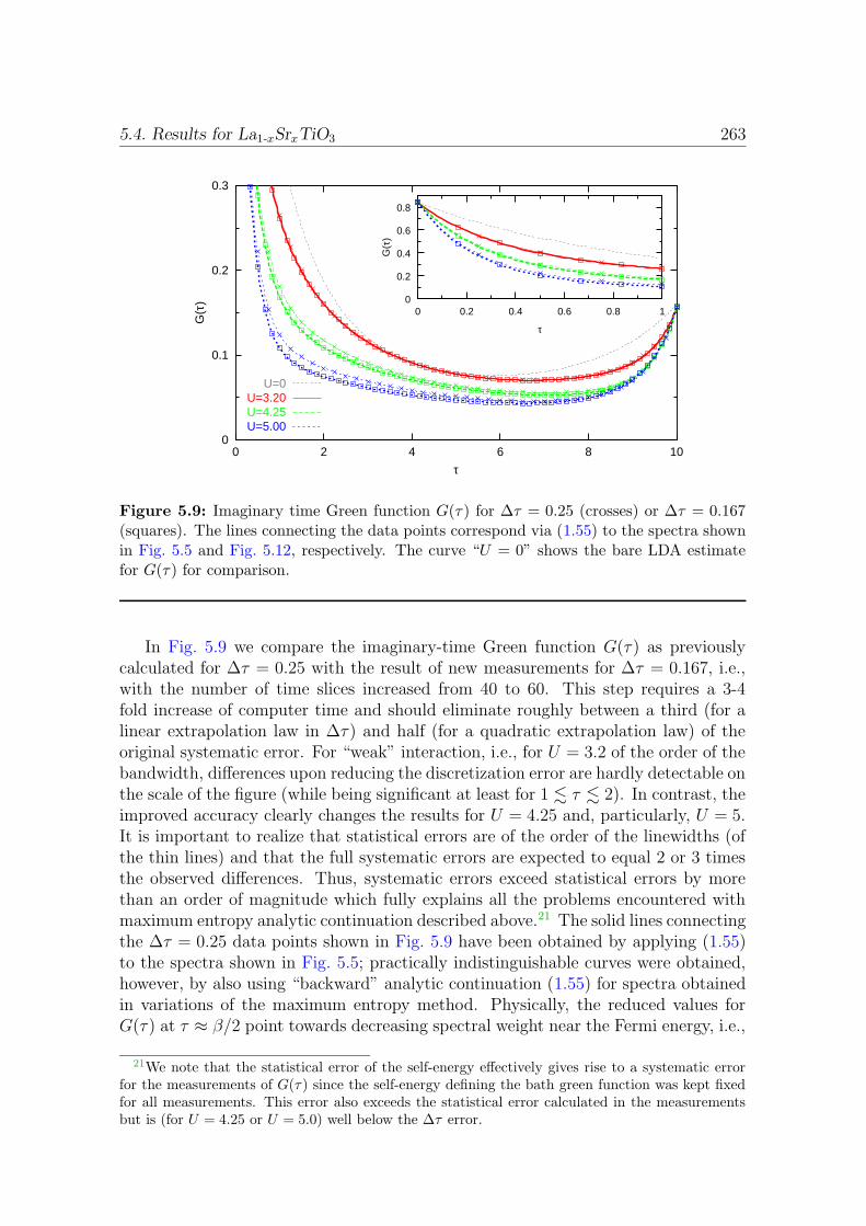
5.4. Results for La1-xSrxTiO3 263
0
0.1
0.2
0.3
0 2 4 6 8 10
G(τ
)
τ
U=0U=3.20U=4.25U=5.00
0
0.2
0.4
0.6
0.8
0 0.2 0.4 0.6 0.8 1
G(τ
)
τ
Figure 5.9: Imaginary time Green function G(τ) for ∆τ = 0.25 (crosses) or ∆τ = 0.167(squares). The lines connecting the data points correspond via (1.55) to the spectra shownin Fig. 5.5 and Fig. 5.12, respectively. The curve “U = 0” shows the bare LDA estimatefor G(τ) for comparison.
In Fig. 5.9 we compare the imaginary-time Green function G(τ) as previouslycalculated for ∆τ = 0.25 with the result of new measurements for ∆τ = 0.167, i.e.,with the number of time slices increased from 40 to 60. This step requires a 3-4fold increase of computer time and should eliminate roughly between a third (for alinear extrapolation law in ∆τ) and half (for a quadratic extrapolation law) of theoriginal systematic error. For “weak” interaction, i.e., for U = 3.2 of the order of thebandwidth, differences upon reducing the discretization error are hardly detectable onthe scale of the figure (while being significant at least for 1 . τ . 2). In contrast, theimproved accuracy clearly changes the results for U = 4.25 and, particularly, U = 5.It is important to realize that statistical errors are of the order of the linewidths (ofthe thin lines) and that the full systematic errors are expected to equal 2 or 3 timesthe observed differences. Thus, systematic errors exceed statistical errors by morethan an order of magnitude which fully explains all the problems encountered withmaximum entropy analytic continuation described above.21 The solid lines connectingthe ∆τ = 0.25 data points shown in Fig. 5.9 have been obtained by applying (1.55)to the spectra shown in Fig. 5.5; practically indistinguishable curves were obtained,however, by also using “backward” analytic continuation (1.55) for spectra obtainedin variations of the maximum entropy method. Physically, the reduced values forG(τ) at τ ≈ β/2 point towards decreasing spectral weight near the Fermi energy, i.e.,
21We note that the statistical error of the self-energy effectively gives rise to a systematic errorfor the measurements of G(τ) since the self-energy defining the bath green function was kept fixedfor all measurements. This error also exceeds the statistical error calculated in the measurementsbut is (for U = 4.25 or U = 5.0) well below the ∆τ error.
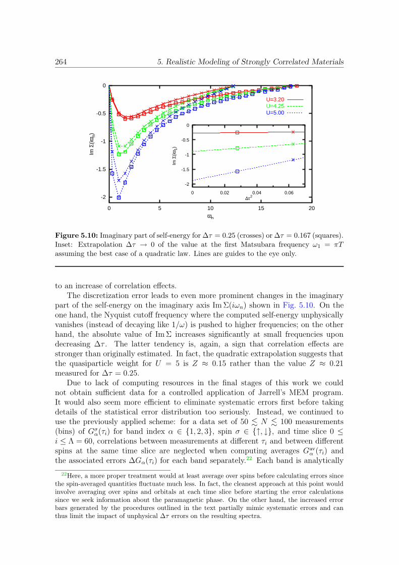
264 5. Realistic Modeling of Strongly Correlated Materials
-2
-1.5
-1
-0.5
0
0 5 10 15 20
Im Σ
(iωn)
ωn
U=3.20U=4.25U=5.00
-2
-1.5
-1
-0.5
0
0 0.02 0.04 0.06
Im Σ
(iω1)
∆τ2
"LaTiO3dtcompself.dat" u ($2**2):(($1==3.2) $2==0.25)?$3:1/0)"" u ($2**2):(($1==3.2) $2==0.167)?$3:1/0)
-0.274658+0.574875*x"" u ($2**2):(($1==4.25) $2==0.25)?$3:1/0)
"" u ($2**2):(($1==4.25) $2==0.167)?$3:1/0)-0.900408+3.93349*x
"" u ($2**2):(($1==5.0) $2==0.25)?$3:1/0)"" u ($2**2):(($1==5.0) $2==0.167)?$3:1/0)
-1.88284+11.1343*x
Figure 5.10: Imaginary part of self-energy for ∆τ = 0.25 (crosses) or ∆τ = 0.167 (squares).Inset: Extrapolation ∆τ → 0 of the value at the first Matsubara frequency ω1 = πTassuming the best case of a quadratic law. Lines are guides to the eye only.
to an increase of correlation effects.The discretization error leads to even more prominent changes in the imaginary
part of the self-energy on the imaginary axis Im Σ(iωn) shown in Fig. 5.10. On theone hand, the Nyquist cutoff frequency where the computed self-energy unphysicallyvanishes (instead of decaying like 1/ω) is pushed to higher frequencies; on the otherhand, the absolute value of Im Σ increases significantly at small frequencies upondecreasing ∆τ . The latter tendency is, again, a sign that correlation effects arestronger than originally estimated. In fact, the quadratic extrapolation suggests thatthe quasiparticle weight for U = 5 is Z ≈ 0.15 rather than the value Z ≈ 0.21measured for ∆τ = 0.25.
Due to lack of computing resources in the final stages of this work we couldnot obtain sufficient data for a controlled application of Jarrell’s MEM program.It would also seem more efficient to eliminate systematic errors first before takingdetails of the statistical error distribution too seriously. Instead, we continued touse the previously applied scheme: for a data set of 50 . N . 100 measurements(bins) of Gσ
α(τi) for band index α ∈ 1, 2, 3, spin σ ∈ ↑, ↓, and time slice 0 ≤i ≤ Λ = 60, correlations between measurements at different τi and between differentspins at the same time slice are neglected when computing averages Gav
α (τi) andthe associated errors ∆Gα(τi) for each band separately.22 Each band is analytically
22Here, a more proper treatment would at least average over spins before calculating errors sincethe spin-averaged quantities fluctuate much less. In fact, the cleanest approach at this point wouldinvolve averaging over spins and orbitals at each time slice before starting the error calculationssince we seek information about the paramagnetic phase. On the other hand, the increased errorbars generated by the procedures outlined in the text partially mimic systematic errors and canthus limit the impact of unphysical ∆τ errors on the resulting spectra.
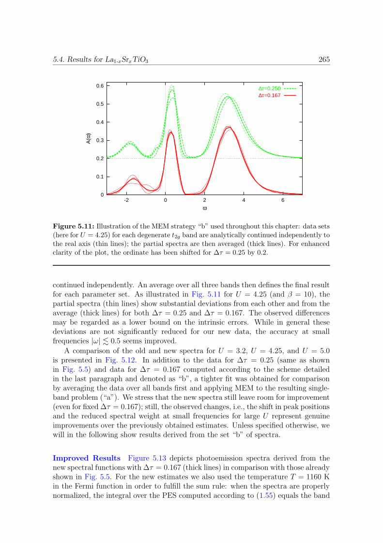
5.4. Results for La1-xSrxTiO3 265
0
0.1
0.2
0.3
0.4
0.5
0.6
-2 0 2 4 6
A(ω
)
ω
∆τ=0.250∆τ=0.167
Figure 5.11: Illustration of the MEM strategy “b” used throughout this chapter: data sets(here for U = 4.25) for each degenerate t2g band are analytically continued independently tothe real axis (thin lines); the partial spectra are then averaged (thick lines). For enhancedclarity of the plot, the ordinate has been shifted for ∆τ = 0.25 by 0.2.
continued independently. An average over all three bands then defines the final resultfor each parameter set. As illustrated in Fig. 5.11 for U = 4.25 (and β = 10), thepartial spectra (thin lines) show substantial deviations from each other and from theaverage (thick lines) for both ∆τ = 0.25 and ∆τ = 0.167. The observed differencesmay be regarded as a lower bound on the intrinsic errors. While in general thesedeviations are not significantly reduced for our new data, the accuracy at smallfrequencies |ω| . 0.5 seems improved.
A comparison of the old and new spectra for U = 3.2, U = 4.25, and U = 5.0is presented in Fig. 5.12. In addition to the data for ∆τ = 0.25 (same as shownin Fig. 5.5) and data for ∆τ = 0.167 computed according to the scheme detailedin the last paragraph and denoted as “b”, a tighter fit was obtained for comparisonby averaging the data over all bands first and applying MEM to the resulting single-band problem (“a”). We stress that the new spectra still leave room for improvement(even for fixed ∆τ = 0.167); still, the observed changes, i.e., the shift in peak positionsand the reduced spectral weight at small frequencies for large U represent genuineimprovements over the previously obtained estimates. Unless specified otherwise, wewill in the following show results derived from the set “b” of spectra.
Improved Results Figure 5.13 depicts photoemission spectra derived from thenew spectral functions with ∆τ = 0.167 (thick lines) in comparison with those alreadyshown in Fig. 5.5. For the new estimates we also used the temperature T = 1160 Kin the Fermi function in order to fulfill the sum rule: when the spectra are properlynormalized, the integral over the PES computed according to (1.55) equals the band

266 5. Realistic Modeling of Strongly Correlated Materials
0
0.1
0.2
0.3
0.4
0.5
-3 -2 -1 0 1 2 3 4 5 6
A(ω
)
ω
U=5.0
0
0.1
0.2
0.3
0.4
0.5
A(ω
)
U=4.25
0
0.1
0.2
0.3
0.4
0.5A
(ω)
U=3.2∆τ=0.25
a: ∆τ=0.167b: ∆τ=0.167
Figure 5.12: Spectra (interacting DOS): new results for ∆τ = 0.167 using variations of theMEM technique (see text) in comparison to the spectra for ∆τ = 0.25 shown in Fig. 5.5.
filling to very high accuracy.23 The increased accuracy makes the peaks at the Fermienergy less prominent; this correlation effect would appear even stronger had bothsets of curves been calculated using the same Fermi function. Furthermore, the shapeand position of the lower Hubbard bands are modified and the peak positions becomemore systematic as a function of U .
The upper part of the interacting DOS is in principle also observable experi-mentally via inverse photoemission, which we model by formally applying (5.23) fornegative temperatures. In this case, the noninteracting eg bands situated above theLDA Fermi energy become very important as is evident in Fig. 5.14. Here, we haveused U = 5.0 and ignored a possible shift of the Fermi energy, which would also shiftthe t2g band relative to the remainder of the spectrum. The total PES includes acontribution associated with the O 2p band which then fills the gap in the t2g con-tribution at about 1 eV. In lack of true inverse PES experiments, we compare to
23The estimates shown in Fig. 5.7, using T ¿ ∆ω = 0.1 eV in the Fermi function, correspondedto significantly lower band fillings. Therefore, they had been rescaled in (Nekrasov et al., 2000).

5.4. Results for La1-xSrxTiO3 267
0
0.02
0.04
0.06
0.08
0.1
-3 -2.5 -2 -1.5 -1 -0.5 0 0.5 1
PE
S In
tens
ity (
stat
es/o
rbita
l)
Energy (eV)
U=3.2U=4.2U=5.0
Figure 5.13: La1-xSrxTiO3 photoemission spectra (x=0.06): LDA+DMFT(QMC) esti-mates for ∆τ = 0.167 and T = 1160 K (thick lines) in comparison to the previouslyobtained results shown in Fig. 5.7 (thin lines). The longer tails at positive energies are dueto our use of T = 1160 K also in the Fermi function (see text).
0
0.2
0.4
0.6
0.8
1
1.2
1.4
0 1 2 3 4 5 6
Inte
nsity
ω
fullTi 3d egTi 3d t2g
O 2pexp: XAS
Figure 5.14: Inverse photoemission: full theoretical estimate and contributions arisingfrom the correlated t2g band as well as uncorrelated eg and O 2p bands in comparison withexperimental XAS data (Abbate et al., 1991). For the theoretical curves, U = 5 eV and afixed Fermi energy (see text) have been assumed.
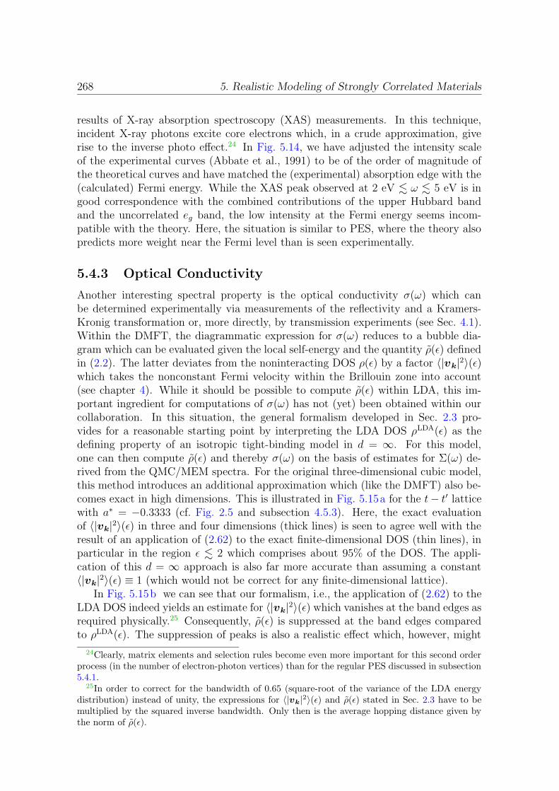
268 5. Realistic Modeling of Strongly Correlated Materials
results of X-ray absorption spectroscopy (XAS) measurements. In this technique,incident X-ray photons excite core electrons which, in a crude approximation, giverise to the inverse photo effect.24 In Fig. 5.14, we have adjusted the intensity scaleof the experimental curves (Abbate et al., 1991) to be of the order of magnitude ofthe theoretical curves and have matched the (experimental) absorption edge with the(calculated) Fermi energy. While the XAS peak observed at 2 eV . ω . 5 eV is ingood correspondence with the combined contributions of the upper Hubbard bandand the uncorrelated eg band, the low intensity at the Fermi energy seems incom-patible with the theory. Here, the situation is similar to PES, where the theory alsopredicts more weight near the Fermi level than is seen experimentally.
5.4.3 Optical Conductivity
Another interesting spectral property is the optical conductivity σ(ω) which canbe determined experimentally via measurements of the reflectivity and a Kramers-Kronig transformation or, more directly, by transmission experiments (see Sec. 4.1).Within the DMFT, the diagrammatic expression for σ(ω) reduces to a bubble dia-gram which can be evaluated given the local self-energy and the quantity ρ(ε) definedin (2.2). The latter deviates from the noninteracting DOS ρ(ε) by a factor 〈|vk|2〉(ε)which takes the nonconstant Fermi velocity within the Brillouin zone into account(see chapter 4). While it should be possible to compute ρ(ε) within LDA, this im-portant ingredient for computations of σ(ω) has not (yet) been obtained within ourcollaboration. In this situation, the general formalism developed in Sec. 2.3 pro-vides for a reasonable starting point by interpreting the LDA DOS ρLDA(ε) as thedefining property of an isotropic tight-binding model in d = ∞. For this model,one can then compute ρ(ε) and thereby σ(ω) on the basis of estimates for Σ(ω) de-rived from the QMC/MEM spectra. For the original three-dimensional cubic model,this method introduces an additional approximation which (like the DMFT) also be-comes exact in high dimensions. This is illustrated in Fig. 5.15a for the t− t′ latticewith a∗ = −0.3333 (cf. Fig. 2.5 and subsection 4.5.3). Here, the exact evaluationof 〈|vk|2〉(ε) in three and four dimensions (thick lines) is seen to agree well with theresult of an application of (2.62) to the exact finite-dimensional DOS (thin lines), inparticular in the region ε . 2 which comprises about 95% of the DOS. The appli-cation of this d = ∞ approach is also far more accurate than assuming a constant〈|vk|2〉(ε) ≡ 1 (which would not be correct for any finite-dimensional lattice).
In Fig. 5.15b we can see that our formalism, i.e., the application of (2.62) to theLDA DOS indeed yields an estimate for 〈|vk|2〉(ε) which vanishes at the band edges asrequired physically.25 Consequently, ρ(ε) is suppressed at the band edges comparedto ρLDA(ε). The suppression of peaks is also a realistic effect which, however, might
24Clearly, matrix elements and selection rules become even more important for this second orderprocess (in the number of electron-photon vertices) than for the regular PES discussed in subsection5.4.1.
25In order to correct for the bandwidth of 0.65 (square-root of the variance of the LDA energydistribution) instead of unity, the expressions for 〈|vk|2〉(ε) and ρ(ε) stated in Sec. 2.3 have to bemultiplied by the squared inverse bandwidth. Only then is the average hopping distance given bythe norm of ρ(ε).
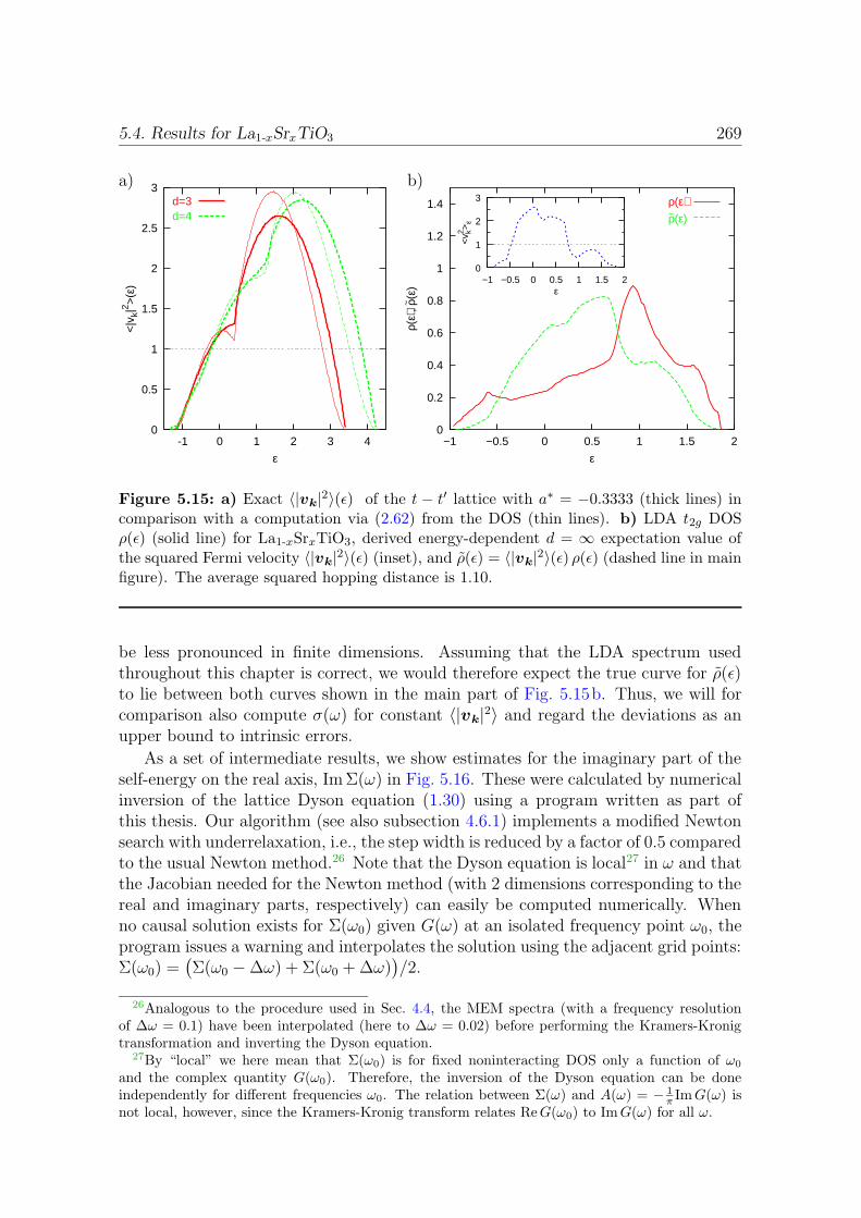
5.4. Results for La1-xSrxTiO3 269
a) b)
0
0.5
1
1.5
2
2.5
3
-1 0 1 2 3 4
<|v
k|2 >
(ε)
ε
d=3d=4
0
0.2
0.4
0.6
0.8
1
1.2
1.4
−1 −0.5 0 0.5 1 1.5 2
ρ(ε)
, ~ ρ(ε)
ε
ρ(ε)~ρ(ε)
0
1
2
3
−1 −0.5 0 0.5 1 1.5 2
<v k2 >
ε
ε
Figure 5.15: a) Exact 〈|vk|2〉(ε) of the t − t′ lattice with a∗ = −0.3333 (thick lines) incomparison with a computation via (2.62) from the DOS (thin lines). b) LDA t2g DOSρ(ε) (solid line) for La1-xSrxTiO3, derived energy-dependent d = ∞ expectation value ofthe squared Fermi velocity 〈|vk|2〉(ε) (inset), and ρ(ε) = 〈|vk|2〉(ε) ρ(ε) (dashed line in mainfigure). The average squared hopping distance is 1.10.
be less pronounced in finite dimensions. Assuming that the LDA spectrum usedthroughout this chapter is correct, we would therefore expect the true curve for ρ(ε)to lie between both curves shown in the main part of Fig. 5.15b. Thus, we will forcomparison also compute σ(ω) for constant 〈|vk|2〉 and regard the deviations as anupper bound to intrinsic errors.
As a set of intermediate results, we show estimates for the imaginary part of theself-energy on the real axis, Im Σ(ω) in Fig. 5.16. These were calculated by numericalinversion of the lattice Dyson equation (1.30) using a program written as part ofthis thesis. Our algorithm (see also subsection 4.6.1) implements a modified Newtonsearch with underrelaxation, i.e., the step width is reduced by a factor of 0.5 comparedto the usual Newton method.26 Note that the Dyson equation is local27 in ω and thatthe Jacobian needed for the Newton method (with 2 dimensions corresponding to thereal and imaginary parts, respectively) can easily be computed numerically. Whenno causal solution exists for Σ(ω0) given G(ω) at an isolated frequency point ω0, theprogram issues a warning and interpolates the solution using the adjacent grid points:Σ(ω0) =
(Σ(ω0 −∆ω) + Σ(ω0 + ∆ω)
)/2.
26Analogous to the procedure used in Sec. 4.4, the MEM spectra (with a frequency resolutionof ∆ω = 0.1) have been interpolated (here to ∆ω = 0.02) before performing the Kramers-Kronigtransformation and inverting the Dyson equation.
27By “local” we here mean that Σ(ω0) is for fixed noninteracting DOS only a function of ω0
and the complex quantity G(ω0). Therefore, the inversion of the Dyson equation can be doneindependently for different frequencies ω0. The relation between Σ(ω) and A(ω) = − 1
π ImG(ω) isnot local, however, since the Kramers-Kronig transform relates ReG(ω0) to ImG(ω) for all ω.
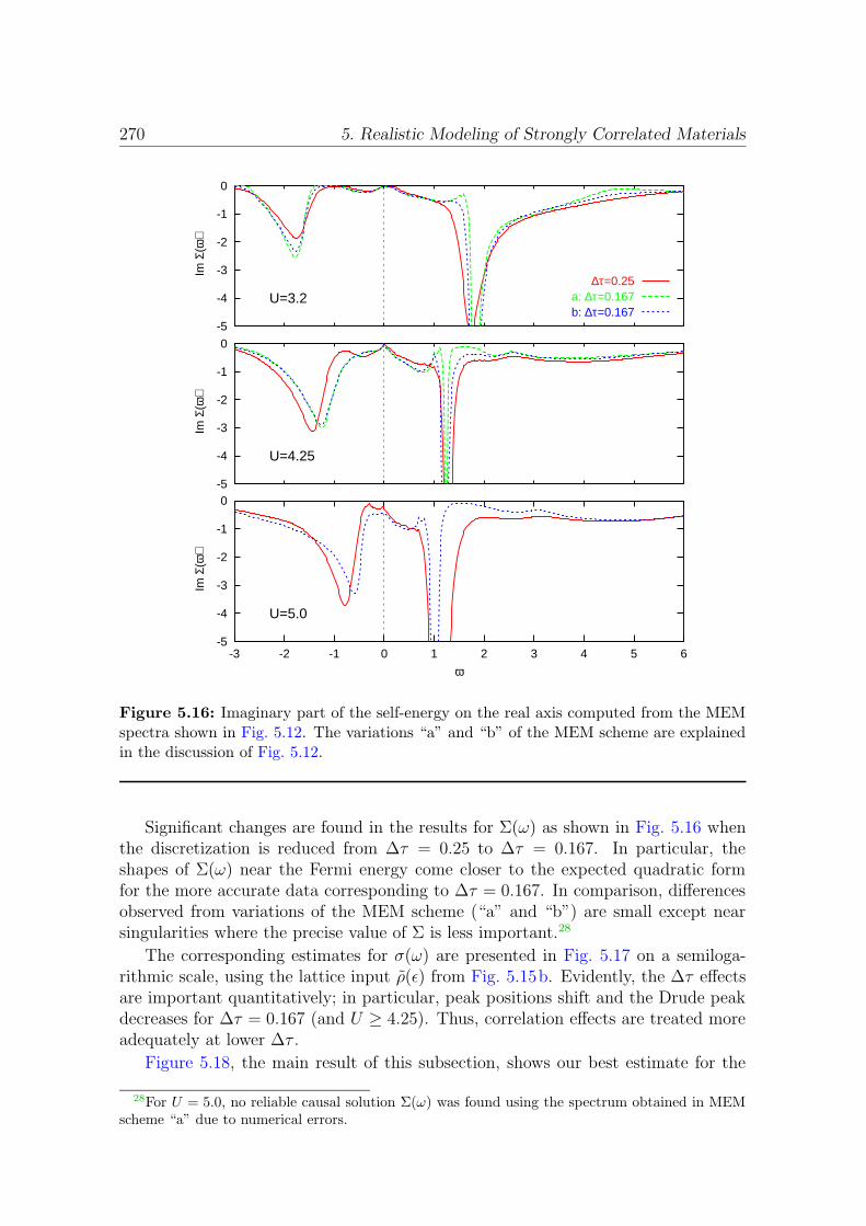
270 5. Realistic Modeling of Strongly Correlated Materials
-5
-4
-3
-2
-1
0
-3 -2 -1 0 1 2 3 4 5 6
Im Σ
(ω)
ω
U=5.0
-5
-4
-3
-2
-1
0
Im Σ
(ω)
U=4.25
-5
-4
-3
-2
-1
0Im
Σ(ω
)
U=3.2∆τ=0.25
a: ∆τ=0.167b: ∆τ=0.167
Figure 5.16: Imaginary part of the self-energy on the real axis computed from the MEMspectra shown in Fig. 5.12. The variations “a” and “b” of the MEM scheme are explainedin the discussion of Fig. 5.12.
Significant changes are found in the results for Σ(ω) as shown in Fig. 5.16 whenthe discretization is reduced from ∆τ = 0.25 to ∆τ = 0.167. In particular, theshapes of Σ(ω) near the Fermi energy come closer to the expected quadratic formfor the more accurate data corresponding to ∆τ = 0.167. In comparison, differencesobserved from variations of the MEM scheme (“a” and “b”) are small except nearsingularities where the precise value of Σ is less important.28
The corresponding estimates for σ(ω) are presented in Fig. 5.17 on a semiloga-rithmic scale, using the lattice input ρ(ε) from Fig. 5.15b. Evidently, the ∆τ effectsare important quantitatively; in particular, peak positions shift and the Drude peakdecreases for ∆τ = 0.167 (and U ≥ 4.25). Thus, correlation effects are treated moreadequately at lower ∆τ .
Figure 5.18, the main result of this subsection, shows our best estimate for the
28For U = 5.0, no reliable causal solution Σ(ω) was found using the spectrum obtained in MEMscheme “a” due to numerical errors.
5.4. Results for La1-xSrxTiO3 271
0.001
0.01
0.1
1
0 1 2 3 4 5 6 7 8
σ(ω
)
ω
U=5.0
0.001
0.01
0.1
1
σ(ω
)
U=4.25
0.001
0.01
0.1
1σ(
ω)
U=3.2∆τ=0.25
a: ∆τ=0.167b: ∆τ=0.167
Figure 5.17: Optical conductivity σ(ω) for La1-xSrxTiO3 using the d = ∞ estimate forρ(ε) depicted in Fig. 5.15b. The variations “a” and “b” of the MEM scheme are explainedin the discussion of Fig. 5.12.
real part of the optical conductivity σ(ω) for U = 3.2, U = 4.25, and U = 5.0(thick lines) at T = 0.1 (using set “b” for ∆τ = 0.167) in comparison with resultsthat the same formalism yields for a constant squared Fermi velocity 〈|vk|2〉. Theinclusion of a nonconstant 〈|vk|2〉(ε) clearly impacts the total spectral weight andits distribution for all choices of the interaction. In general, features become morepronounced. Quantitatively, this effect becomes less important for strong interac-tions: at U = 5, the relative error associated with a neglect of the energy dependenceof 〈|vk|2〉(ε) never exceeds about 20%. From this fact we conclude that also a fullfinite-dimensional LDA evaluation of ρ(ε) or, equivalently, of 〈|vk|2〉(ε) would notlead to dramatic changes compared to our estimate. Therefore, we regard our resultfor U = 5 as a reasonable LDA+DMFT(QMC) estimate for the 3d t2g contributionto the optical conductivity of La1-xSrxTiO3 with doping x = 0.06. On the otherhand, much more reliable results for all observables discussed in this section couldbe expected when using a state-of-the-art QMC program that does not suffer fromlarge ∆τ errors due to an inefficient implementation of the Fourier-transformation
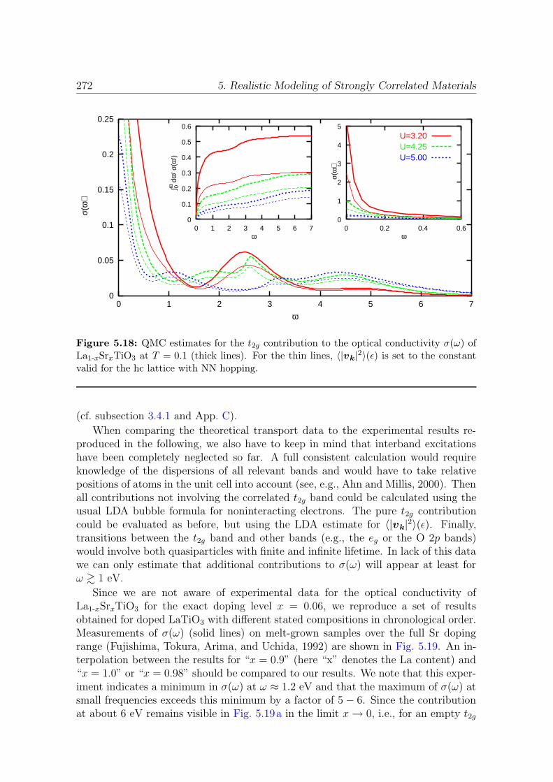
272 5. Realistic Modeling of Strongly Correlated Materials
0
0.05
0.1
0.15
0.2
0.25
0 1 2 3 4 5 6 7
σ(ω
)
ω
0
1
2
3
4
5
0 0.2 0.4 0.6
σ(ω
)
ω
U=3.20U=4.25U=5.00
0
0.1
0.2
0.3
0.4
0.5
0.6
0 1 2 3 4 5 6 7
∫ 0ω d
ω’ σ
(ω’)
ω
Figure 5.18: QMC estimates for the t2g contribution to the optical conductivity σ(ω) ofLa1-xSrxTiO3 at T = 0.1 (thick lines). For the thin lines, 〈|vk|2〉(ε) is set to the constantvalid for the hc lattice with NN hopping.
(cf. subsection 3.4.1 and App. C).
When comparing the theoretical transport data to the experimental results re-produced in the following, we also have to keep in mind that interband excitationshave been completely neglected so far. A full consistent calculation would requireknowledge of the dispersions of all relevant bands and would have to take relativepositions of atoms in the unit cell into account (see, e.g., Ahn and Millis, 2000). Thenall contributions not involving the correlated t2g band could be calculated using theusual LDA bubble formula for noninteracting electrons. The pure t2g contributioncould be evaluated as before, but using the LDA estimate for 〈|vk|2〉(ε). Finally,transitions between the t2g band and other bands (e.g., the eg or the O 2p bands)would involve both quasiparticles with finite and infinite lifetime. In lack of this datawe can only estimate that additional contributions to σ(ω) will appear at least forω & 1 eV.
Since we are not aware of experimental data for the optical conductivity ofLa1-xSrxTiO3 for the exact doping level x = 0.06, we reproduce a set of resultsobtained for doped LaTiO3 with different stated compositions in chronological order.Measurements of σ(ω) (solid lines) on melt-grown samples over the full Sr dopingrange (Fujishima, Tokura, Arima, and Uchida, 1992) are shown in Fig. 5.19. An in-terpolation between the results for “x = 0.9” (here “x” denotes the La content) and“x = 1.0” or “x = 0.98” should be compared to our results. We note that this exper-iment indicates a minimum in σ(ω) at ω ≈ 1.2 eV and that the maximum of σ(ω) atsmall frequencies exceeds this minimum by a factor of 5− 6. Since the contributionat about 6 eV remains visible in Fig. 5.19a in the limit x→ 0, i.e., for an empty t2g

5.4. Results for La1-xSrxTiO3 273
a) b)
Figure 5.19: a)+b) Optical conductivity σ(ω) (solid lines) as measured by Fujishima et al.(1992) at T ≈ 300 K. Since x here corresponds to the t2g band filling, x ≈ 1 is the stronglycorrelated limit. b) Low-energy part with a linear scale and electronic energy-loss functionIm (−1/ε) (dashed lines).
band, a large part of it must be due to excitations involving other bands. Note thata tail of this contribution extends down to about 1 eV. The width of the remnant ofa Drude peak is even much larger than found in our high-temperature calculationswhich points towards strong disorder. Curve “C” in Fig. 5.20a shows σ(ω) measuredfor La1−xSrTiO3 with x ≈ 0.07 (Crandles et al., 1994). Here, a sharp Drude peakis observed at very low frequency ω . 0.1 eV while for larger frequencies the curveis almost flat. If this is significant, disorder effects seem to be less important in thiscase.
In both cases, there is no obvious agreement with any of the results shown inFig. 5.18, i.e., with the (intraband absorption only) LDA+DMFT theory. While theminimum experimentally seen in σ(ω) slightly above 1 eV would find correspondencein the theoretical results for U = 4.25, the computed Drude weight seems still toolarge even for U = 5.0.
The remaining three figures for σ(ω) in doped titanates are all due to Tokura’sgroup. While Fig. 5.20b relates to LaTiO3+δ/2 and shows noisy peaks at low fre-quencies (Okimoto et al., 1995), a curve for La1-xSrxTiO3 with x = 0.1 has beenadded to a selection of the same curves in Fig. 5.21a (Katsufuji et al., 1995). In thelatter diagram, also the low-frequency parts have been removed. Finally, Fig. 5.21bapparently shows the same measured data (solid lines) as Fig. 5.21a, but now ex-
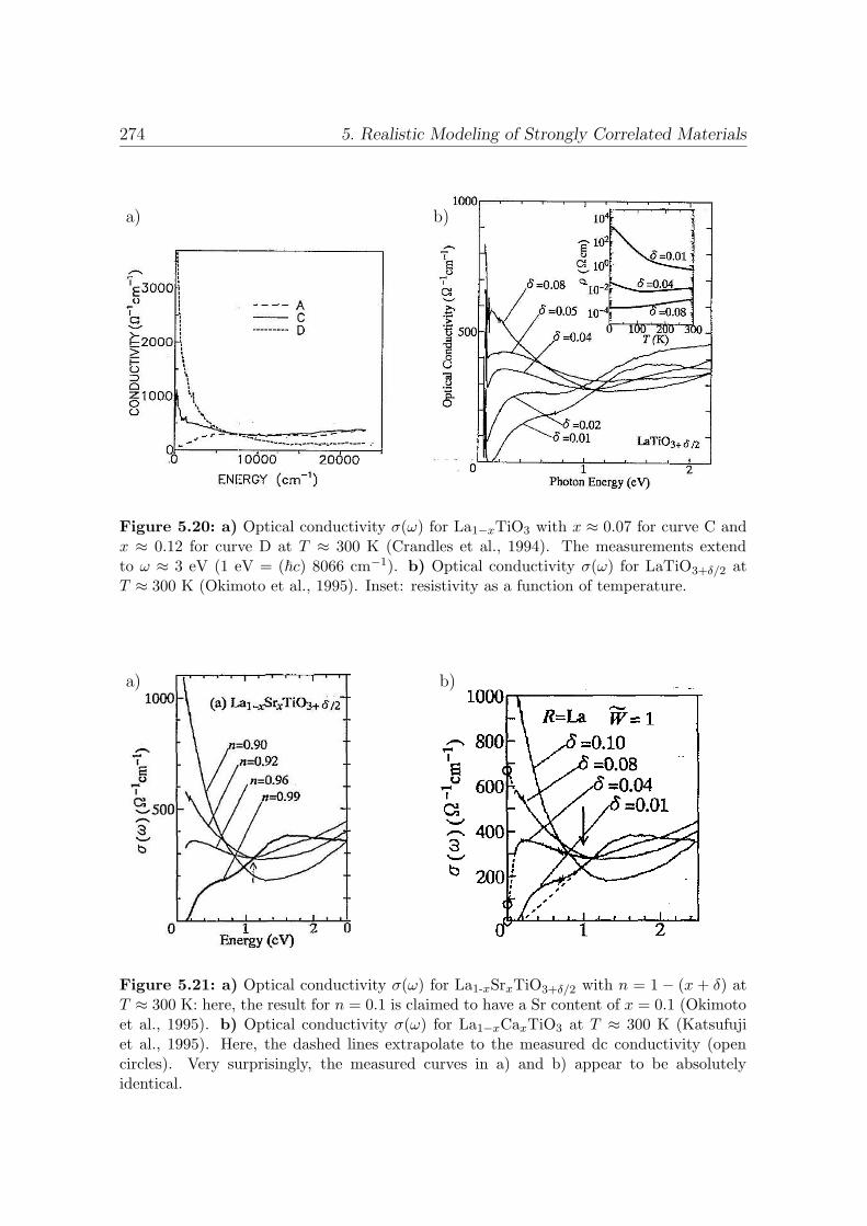
274 5. Realistic Modeling of Strongly Correlated Materials
a) b)
Figure 5.20: a) Optical conductivity σ(ω) for La1−xTiO3 with x ≈ 0.07 for curve C andx ≈ 0.12 for curve D at T ≈ 300 K (Crandles et al., 1994). The measurements extendto ω ≈ 3 eV (1 eV = (~c) 8066 cm−1). b) Optical conductivity σ(ω) for LaTiO3+δ/2 atT ≈ 300 K (Okimoto et al., 1995). Inset: resistivity as a function of temperature.
a) b)
Figure 5.21: a) Optical conductivity σ(ω) for La1-xSrxTiO3+δ/2 with n = 1 − (x + δ) atT ≈ 300 K: here, the result for n = 0.1 is claimed to have a Sr content of x = 0.1 (Okimotoet al., 1995). b) Optical conductivity σ(ω) for La1−xCaxTiO3 at T ≈ 300 K (Katsufujiet al., 1995). Here, the dashed lines extrapolate to the measured dc conductivity (opencircles). Very surprisingly, the measured curves in a) and b) appear to be absolutelyidentical.
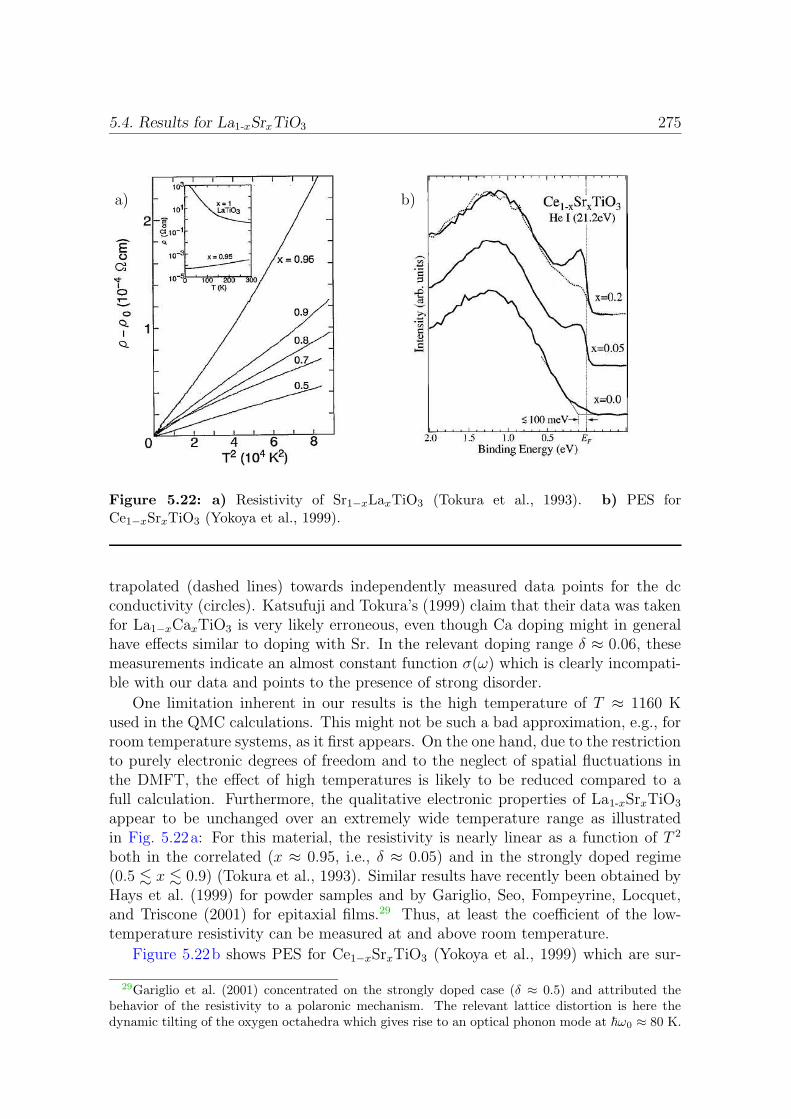
5.4. Results for La1-xSrxTiO3 275
a) b)
Figure 5.22: a) Resistivity of Sr1−xLaxTiO3 (Tokura et al., 1993). b) PES forCe1−xSrxTiO3 (Yokoya et al., 1999).
trapolated (dashed lines) towards independently measured data points for the dcconductivity (circles). Katsufuji and Tokura’s (1999) claim that their data was takenfor La1−xCaxTiO3 is very likely erroneous, even though Ca doping might in generalhave effects similar to doping with Sr. In the relevant doping range δ ≈ 0.06, thesemeasurements indicate an almost constant function σ(ω) which is clearly incompati-ble with our data and points to the presence of strong disorder.
One limitation inherent in our results is the high temperature of T ≈ 1160 Kused in the QMC calculations. This might not be such a bad approximation, e.g., forroom temperature systems, as it first appears. On the one hand, due to the restrictionto purely electronic degrees of freedom and to the neglect of spatial fluctuations inthe DMFT, the effect of high temperatures is likely to be reduced compared to afull calculation. Furthermore, the qualitative electronic properties of La1-xSrxTiO3
appear to be unchanged over an extremely wide temperature range as illustratedin Fig. 5.22a: For this material, the resistivity is nearly linear as a function of T 2
both in the correlated (x ≈ 0.95, i.e., δ ≈ 0.05) and in the strongly doped regime(0.5 . x . 0.9) (Tokura et al., 1993). Similar results have recently been obtained byHays et al. (1999) for powder samples and by Gariglio, Seo, Fompeyrine, Locquet,and Triscone (2001) for epitaxial films.29 Thus, at least the coefficient of the low-temperature resistivity can be measured at and above room temperature.
Figure 5.22b shows PES for Ce1−xSrxTiO3 (Yokoya et al., 1999) which are sur-
29Gariglio et al. (2001) concentrated on the strongly doped case (δ ≈ 0.5) and attributed thebehavior of the resistivity to a polaronic mechanism. The relevant lattice distortion is here thedynamic tilting of the oxygen octahedra which gives rise to an optical phonon mode at ~ω0 ≈ 80 K.
276 5. Realistic Modeling of Strongly Correlated Materials
prisingly similar to the corresponding plot for La1-xSrxTiO3 shown in Fig. 5.7. Thisdemonstrates that our results may apply to a relatively large class of materials andthat, within this class, La1-xSrxTiO3 may not be the system best described by ourapproach.
5.5 Conclusion
In this chapter, we have given an introduction to the ab initio density functionaltheory, to its local density approximation (LDA), and to the hybrid LDA+DMFTmethod in enough detail to expose the various inherent approximations. We have pre-sented published results (Nekrasov et al., 2000) for La1-xSrxTiO3; the relatively goodagreement of the computed photoemission data with experiments clearly demon-strates the significant improvement over conventional LDA calculations. We havealso discussed some subtleties of the theoretical treatment of photoemission spectra(PES) and have demonstrated the numerical significance of an error in the PES codewhich we had discovered and corrected.
New results obtained by Nekrasov for the doping dependence of the quasiparticleweight and of the susceptibility of La1-xSrxTiO3 (unpublished) and a planned jointpublication (Nekrasov, Blumer, Held, Anisimov, and Vollhardt, 2001) as well as ourexperiences from treating the metal insulator transition of the half-filled Hubbardmodel (cf. chapter 3) using the uncorrected QMC code prompted us to questionthe reliability of the LDA+DMFT(QMC) results in the strongly correlated regime.Therefore, we have repeated all original calculations using an increased number ofimaginary time slices in QMC (∆τ = 0.167 instead of ∆τ = 0.25) and testing vari-ations of the maximum entropy method (MEM). As expected, we found significantcorrections to the quasiparticle weights and also to the MEM spectra. Our moreaccurate treatment also leads to a slightly reduced relative weight in the PES nearthe Fermi energy which is, however, still too high in comparison with experiment.Furthermore, we have computed x-ray absorption (XAS) spectra. While the overallagreement with experiment was seen to be reasonable when including the contribu-tions of Ti eg and O 2p bands (in addition to the Ti t2g bands), the weight at theFermi energy was again overestimated by theory.
Finally, we have computed the first LDA+DMFT(QMC) estimate of the Ti t2gcontribution to the optical conductivity σ(ω) of La1-xSrxTiO3. One prerequisite forthis calculation was the development of a program for the inversion of the general k-integrated Dyson equation. In lack of momentum resolved LDA data, we also neededto determine the effect of a nonconstant Fermi velocity by application of the generaldispersion formalism developed in Sec. 2.3 to the LDA density of states. A detailedcomparison of the numerical results with experiment is difficult. On the one hand,experimental results for σ(ω) differ greatly with respect to the presence or widthof a Drude peak. On the other hand, contributions of orbitals not included in ourtheory can be expected to be significant. Taking these uncertainties into account, theoverall agreement seems reasonable; again, the most prominent discrepancy is thatthe theory predicts too much weight at small frequencies.

5.5. Conclusion 277
One unrealistic aspect of all LDA+DMFT(QMC) calculations presented in thischapter was the high temperature T ≈ 1160 K. A reduction of the simulation tem-perature to room temperature would be desirable; such a project is clearly realistic,in particular when using an improved QMC code (cf. App. C) for which the dis-cretization ∆τ = 0.25 is sufficiently accurate. One might also want to investigatethe influence of non-uniform on-site coupling terms, the importance of hybridizationterms in a full-Hamiltonian calculation, or the impact of the orthorhombic distortion.
We conclude that the LDA+DMFT(QMC) treatment is vastly superior over thesole application of LDA already at the present stage. Still, the material La1-xSrxTiO3
is less metallic at x = 0.06 than the theory predicts. If this finding holds up inimprovements of the theoretical treatment and in experiments which are more bulk-sensitive, the remaining discrepancies may be due to disorder (which is clearly present,but should be washed out since Ti has 8 La/Sr nearest neighbors) or to (precursorsof) antiferromagnetic order.

278 5. Realistic Modeling of Strongly Correlated Materials
279
Summary
The characterization of a material as metallic or insulating, the study of transitionsbetween such states and the development of suitable models is clearly of great fun-damental and practical interest. The one-band Hubbard model is a conceptionallyrelatively simple model which is potentially relevant in this context since its pri-mary parameter, the on-site interaction U triggers a transition or a crossover frommetallic behavior at small U to insulating behavior at large U and half filling. Areduction of complexity of this model is achieved by the dynamical mean-field theory(DMFT); due to its nonperturbative character, this method is reliable in the rangeof interest, i.e., for intermediate to strong coupling. The resulting model certainlymisses important properties of specific materials such as V2O3; nevertheless, it is agood candidate for controlled numerical studies of the more abstract metal-insulatortransition (MIT) problem.
We have presented quantum Monte Carlo (QMC) results for a fully frustratedversion of the Hubbard model and constructed its phase diagram. We have resolveda controversy regarding the existence and extent of the MIT coexistence region andhave succeeded in the precise determination of the first-order transition line; a taskthat was previously considered too difficult for numerically exact methods. The newmethods employed for this purpose and a more direct (and yet untested) approachdeveloped in this work should prove fruitful for broader application in the future.Further research will also profit from our discovery and correction of problems insome implementations of the QMC method.
The MIT phase diagram Fig. 3.50, a main result of this work, clearly does notrepresent a complete scenario for any material featuring a MIT. This follows alreadyfrom the finite (and large) entropy predicted in the insulating ground state whichviolates Nernst’s law. This contradiction may to some degree be regarded as an arti-fact of the DMFT limit: For any fixed disorder distribution and finite hopping range,long-range order is expected to set in below some critical temperature in any finitedimension d. A more realistic and consistent DMFT description is possible when thelow-temperature phase is ordered already in d = ∞, i.e., for partial frustration. Wehave discussed the qualitative implications of variable frustration in the (nongeneric)case that the properties of the paramagnetic phase remain unchanged. The questionwhether the topology of the phase diagram of V2O3 (with a first-order paramagneticmetal-insulator transition and an antiferromagnetic low-temperature phase) can bereproduced for a lattice with realistic frustration is still open.
The theory of transport in infinite dimensions was previously restricted to thehypercubic lattice (or anisotropic stacked lattices) with nearest-neighbor hopping.
280 Summary
We have generalized the formalism and derived explicit general expressions for theoptical f -sum rule. We have constructed the first regular lattice with finite (semi-elliptic) band edges in d = ∞ and have thus obtained the first DMFT results forcoherent and isotropic transport compatible with a semi-elliptic density of states.
We have reported on progress in the realistic modeling of strongly correlated elec-tron systems using the hybrid LDA+DMFT method. This recently developed methodstarts with the ab initio density functional theory and treats the missing correlationswithin DMFT. Evaluating the resulting multi-band problem using QMC, we havecomputed photoemission and x-ray absorption spectra for the transition metal ox-ide La1-xSrxTiO3. The results represent a significant improvement over conventionalLDA calculations. We have discussed the impact of the QMC discretization errorand computed a first estimate of the t2g contribution to the optical conductivity.
The unifying project of this thesis has been the modeling of strongly correlatedelectron systems in the vicinity of a metal-insulator transition by application of thedynamical mean-field theory which becomes exact in the limit of infinite dimension-ality. Within this project, we have studied single-band as well as multi-band models,pursued both pure model Hamiltonian approaches and the ab initio LDA+DMFTapproach and computed both local and transport properties. A large amount of nu-merical work, i.e., the planning, organization, and analysis of several thousand QMCsimulations using tens of thousands of hours of supercomputer time was clearly es-sential for obtaining the accurate results which we have presented in this thesis.Furthermore, we have written a large number of computer programs and have mod-ified and extended some others. Many of our results, however, could not have beenobtained without the development or improvement of methods and formalisms aswell as analytical calculations. It is this more theoretical than numerical aspect ofour work which we found particularly rewarding.
281
Appendix A
Additions to “Models andMethods”
A.1 Extensions of the Hubbard Model
The one-band Hubbard model represents a highly idealized view of strongly correlatedmaterials. Some of its shortcomings are best characterized by writing down minimalmodel extensions which could be used for adding the missing physics. While most ofthe extensions collected in this section will not be used for actual calculations in thisthesis, we will discuss the implications of extended hopping in chapter 2 and study a3-band model based on LDA input data in chapter 5.
The applicability of the one-band Hubbard model to d or f electron systems isa priori questionable since the partially filled bands correspond to atomic orbitalswhich are 5-fold and 7-fold degenerate (for each spin direction), respectively. Whilebands in a lattice are more complicated than orbitals of isolated atoms, the remainingdegeneracy can be inferred from symmetry considerations alone. Often it is useful toconsider a cubic representation of the angular part of atomic d orbitals,
|dxy〉 ∝ (|2, 2〉 − |2,−2〉) , |dyz〉 ∝ (|2, 1〉+ |2,−1〉) , |dzx〉 ∝ (|2, 1〉 − |2,−1〉)|dx2−y2〉 ∝ (|2, 2〉+ |2,−2〉) , |d3z2−r2〉 ∝ |2, 0〉, (A.1)
expressed in terms of eigenfunctions of the angular momentum operator,
l2|l,m〉 = ~2l(l + 1)|l,m〉, lz|l,m〉 = ~m|l,m〉 . (A.2)
In lattices with cubic symmetry the five d orbitals are energetically split into the t2gorbitals (|dxy〉, |dyz〉, |dzx〉) and the eg orbitals (|dx2−y2〉, |d3z2−r2〉), which give riseto one threefold degenerate and one twofold degenerate band, respectively. Lowersymmetry can lift the remaining degeneracies; e.g., in the trigonal case the t2g orbitalsare further split into one nondegenerate a1g and one twofold degenerate eπg band.Thus, it is possible that in some d systems only one band crosses or touches theFermi surface which then justifies the one-band assumption made in subsection 1.1.4and used in chapter 3. In general, however, the inclusion of several orbitals per siteis important. An SU(2)-invariant generalization of the Hubbard model where the
282 A. Additions to “Models and Methods”
interaction is still local but the valence band is degenerate then contains additionalcoupling terms1 (Anderson, 1961; Dworin and Narath, 1970)
Hm-band = −t∑
〈ij〉,νσc†iνσ cjνσ + U
∑
iν
niν↑niν↓
+V0
∑
i;ν<ν′;σσ′
niνσniν′σ′ + F0
∑
i;ν<ν′;σσ′
c†iνσ c†iν′σ′ ciνσ′ ciν′σ, (A.3)
where ν,ν ′ (with 1 ≤ ν ≤ m, 1 ≤ ν ′ ≤ m) are band indices. The exchange termparameterized by the Hund’s rule coupling F0 can be rewritten as
HF0= −2F0
∑
i,ν<ν′
(
Siν · Siν′ +1
4niνniν′
)
(A.4)
with Siν = 12
∑
σσ′ c†iνστ σσ′ ciνσ′ being the spin operator for orbital ν at site i and the
Pauli matrices τ σσ′ . In quantum Monte Carlo (QMC) simulations, the spin-flippingterms implicit in (A.4) lead to a numeric (minus-sign) problem. Therefore, one hereusually replaces the Heisenberg interaction part of (A.4) by an Ising-type interactionat the cost of breaking the SU(2) symmetry (Motome and Imada, 1997; Held andVollhardt, 1998). Since sziν s
ziν′ = σσ′niνσniν′σ′/4 = (2δσσ′ − 1) niνσniν′σ′/4, one can
write this modified multi-band Hubbard Hamiltonian as
Hzm-band =
∑
〈ij〉,νσεkν c
†kν ckν + U
∑
iν
niν↑niν↓ +∑
i;ν<ν′;σσ′
(V0 − δσσ′F0) niνσniν′σ′ . (A.5)
The interaction U between electrons within each orbital is always larger than theinterorbital density-density interaction V0. The smaller exchange coupling F0 cantrigger ferromagnetic and (possibly coexisting) orbital order.2
While in general the inclusion of different nondegenerate bands involves an ad-ditional large number of parameters, one can model (and simulate using QMC, e.g.,within the DMFT) the influence of a half-filled, locally polarized and relatively inertsubband as observed in manganites by adding a Kondo-type interaction between theitinerant electrons and some spin degree of freedom, −2
∑
ν
∑
i siν · Si. Here, siν are
the spin operators for the itinerant twofold degenerate eg band while Si models alocalized spin-3/2 originating from the t2g band (Held and Vollhardt, 2000).
An additional complication in compounds is the presence of several inequivalentions per unit cell. Such systems can be modeled microscopically by introducing dif-ferent on-site energies, Coulomb interactions, and hopping matrix elements within aunit cell or more phenomenologically by using renormalized hopping matrix elementsbetween just a subset of orbitals (while others are integrated out). One example of the
1Here, an on-site pair hopping term which only contributes when one orbital is doubly andanother singly occupied is neglected (Held and Vollhardt, 1998).
2In the application of the LDA+DMFT method in chapter 5 we will set U = V0 and F0 = 0;in the absence of long range order and for small filling n . 1 the resulting error is not expected toexceed other sources of errors. In general, local exchange terms only become negligible for extendedorbitals (an extreme case being valence molecular orbitals in C60 Fullerides).
A.1. Extensions of the Hubbard Model 283
former approach is the “Emery model” or “Varma-Schmitt-Rink-Abrahams model”for electron holes in the copper oxide planes in high-Tc superconductors (Varma,Schmitt-Rink, and Abrahams, 1987; Emery, 1987)3
Hsc = −tpd∑
〈i,j〉,ν,σ(p†jνσdiσ + h.c.)− tpp
∑
〈j,j′〉,ν,σ(p†jνσpj′νσ + h.c.) + εd
∑
i
ndi + εp∑
jν
npjν
+Ud∑
i
ndi↑ndi↓ + Up
∑
jν
npjν↑npjν↓ + V
∑
〈ij〉,νndi n
pjν . (A.6)
The latter, more phenomenological approach is used for modeling the compoundLa1-xSrxTiO3 using an explicit treatment of the Ti 3d t2g orbitals only in chapter 5.
Since the restriction to local interactions in the Hubbard model is a crude ap-proximation to the Coulomb interaction, one may expect significant improvementsby including nearest-neighbor terms of the Coulomb interaction. For a one-bandmodel, these may be written in the form (Hirsch, 1989; Strack and Vollhardt, 1994)
V NN1-band =
∑
〈i,j〉
[
V ninj − 2F (SiSj +1
4ninj)
+X∑
σ
(c†iσ cjσ + h.c.)(ni−σ + nj−σ) + F ′(c†i↑c†i↓cj↓cj↑ + h.c.)
]
. (A.7)
Here, the V term and the F term are completely analogous to the onsite interac-tions between orbitals in (A.3), while the additional terms involve density-dependenthopping (X) and pair hopping (F ′). These nearest-neighbor contributions of theCoulomb interactions can, e.g., drive ferromagnetism (Hirsch, 1989; Kollar, Strack,and Vollhardt, 1996; Blumer, 1996; Wahle et al., 1998), charge density waves, phaseseparation, or superconductivity (Hirsch and Marsiglio, 2000).
Disorder is always present to some degree in real materials, in particular in dopedsystems (as considered in chapter 5), and is potentially very important, e.g., in thecontext of Anderson localization. A straightforward generalization of the one-bandHubbard model leads to
Hdisorder =∑
iσ
(εi − µ) niσ+∑
〈i,j〉,σtij
(
c†iσ cjσ + h.c.)
+∑
i
Ui(ni↑−1
2)(ni↓−
1
2), (A.8)
where site-diagonal terms, i.e., the lattice potentials εi and the Coulomb interactionUi and/or the (intersite) hopping terms tij may be allowed to vary [for a treatmentwithin DMFT, see, e.g., Dobrosavljevic and Kotliar (1993) and Ulmke (1998)].
The inclusion of phonons is possible in terms of the Holstein-Hubbard model, inwhich the Hubbard model is supplemented by the electron-phonon interaction plusa phonon energy (Holstein, 1959; Zhong and Schuttler, 1992; Freericks and Jarrell,1995b)
HH-H = HHub + g∑
i
Ri(ni↑ + ni↓ − 1) +1
2
∑
i
(P 2i
M+MΩ2R2
i
)
. (A.9)
3Here, i and j denote the unit cell for Cu 3dx2−y2 orbitals and O 2px or 2py orbitals, respectively.The orbital index ν = x or ν = y distinguishes the oxygen orbitals (living on different sites);unrestricted summation over omitted spin indices is implied.

284 A. Additions to “Models and Methods”
Here, Ri (Pi) label the phonon position (momentum) at site i, g is a coupling strength,M is the phonon mass and Ω its frequency.4
Finally, the relativistic spin-orbit interaction can be approximately reintroducedin the form
HSO = ξ∑
νν′σσ′
〈νσ|L · S|ν ′σ′〉c†νσcν′σ′ , (A.10)
where L is the angular momentum operator, S the vector of Pauli matrices, andthe parameter ξ depends on the system (see, e.g., Bruno, 1993; Harle, 2000). In thepresence of magnetic order, this interaction may lead to an easy or hard axis. WithinDMFT, the behavior of antiferromagnetic systems with a strong easy axis can alsobe modeled phenomenologically by restricting local spin moments to point along thisaxis which then leads to metamagnetic phase transitions of both first and second orderupon variation of an external magnetic field (Held, Ulmke, and Vollhardt, 1996; Held,Ulmke, Blumer, and Vollhardt, 1997).
A.2 Characterization of Generic Momenta
In the following, we will first extend the definition of nongeneric momenta given insubsection 1.2.2 to finite dimensions, then show that in all dimensions nongenericmomenta can be characterized as being close to the origin 0 or to the antiferromag-netic wave vector Q and, finally, draw some conclusions for the d → ∞ limit of thehypercubic lattice and the DMFT in general.
In the following, we will exploit that the expression ηq = limd→∞1d
∑dα=1 cos(qα)
introduced in the context of (1.23) for the d =∞ hc lattice naturally extends to finitedimensions. Since ηq always varies in the range [−1, 1] and ηq 6= 0 defines nongenericvectors q in d = ∞, one can identify vectors q with |ηq| > η0 (for any η0 > 0)with strong momentum correlation in any finite dimension d and loosely call themnongeneric, too. Furthermore, we can estimate ηq from the vector norm |q| whichfor momenta in the first Brillouin zone, unit lattice spacing a = 1, and dimension dvaries between |0| = 0 and |Q| = π
√d:
ηq = −1 +1
d
d∑
α=1
(1− cos(qα)) ≤|q|22d− 1 (A.11)
Therefore, η is strictly negative for all momenta inside a hypersphere of radius√
2dwhile η < −0.5 for momenta |q| <
√d. Analogously, η > 0 (η > 0.5) for the
corresponding hyperspheres around Q. Thus, we have identified convex sets of “non-generic” momenta illustrated in Fig. A.1a which are associated with strong energeticcorrelations via (1.23) and which acquire εq = −∞ (εq =∞) in the limit d→∞ onthe hc lattice. In Fig. A.1b, we show the probability distribution of ηq for d = 1, 2, 3 as
4In principle, “phonon coordinate” can be translated as “ion coordinate” (which is d-dimensional). Note, however, that the single Einstein phonon mode considered here only has asingle coordinate, i.e., is one-dimensional. A generalization to (anisotropic) d-dimensional couplingwould require the inclusion of several phonon frequencies.
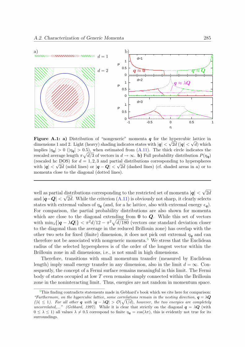
A.2. Characterization of Generic Momenta 285
a) b)d = 1
d = 2
0
0.5
1
-1 -0.5 0 0.5 1
P
η
d=3
0
0.5
1P
d=2
0
0.5
1P
d=1
q ≈ 0 q ≈ Q
q ≈ λQ/
Figure A.1: a) Distribution of “nongeneric” momenta q for the hypercubic lattice indimensions 1 and 2. Light (heavy) shading indicates states with |q| <
√2d (|q| <
√d) which
implies |ηq| > 0 (|ηq| > 0.5), when estimated from (A.11). The thick circle indicates therescaled average length π
√
d/3 of vectors in d→∞. b) Full probability distribution P (ηq)(rescaled hc DOS) for d = 1, 2, 3 and partial distributions corresponding to hypersphereswith |q| <
√2d (solid lines) or |q −Q| <
√2d (dashed lines) (cf. shaded areas in a) or to
momenta close to the diagonal (dotted lines).
well as partial distributions corresponding to the restricted set of momenta |q| <√
2dand |q−Q| <
√2d. While the criterion (A.11) is obviously not sharp, it clearly selects
states with extremal values of ηq (and, for a hc lattice, also with extremal energy εq).For comparison, the partial probability distributions are also shown for momentawhich are close to the diagonal extending from 0 to Q. While this set of vectorswith minλ|q − λQ| < π2d/12 − π2
√
d/180 (vectors one standard deviation closerto the diagonal than the average in the reduced Brillouin zone) has overlap with theother two sets for fixed (finite) dimension, it does not pick out extremal ηq and cantherefore not be associated with nongeneric momenta.5 We stress that the Euclideanradius of the selected hyperspheres is of the order of the longest vector within theBrillouin zone in all dimensions, i.e., is not small in high dimensions.
Therefore, transitions with small momentum transfer (measured by Euclideanlength) imply small energy transfer in any dimension, also in the limit d =∞. Con-sequently, the concept of a Fermi surface remains meaningful in this limit. The Fermibody of states occupied at low T even remains simply connected within the Brillouinzone in the noninteracting limit. Thus, energies are not random in momentum space.
5This finding contradicts statements made in Gebhard’s book which we cite here for comparison:“Furthermore, on the hypercubic lattice, some correlations remain in the nesting direction, q = λQ(|λ| ≤ 1). For all other q with |q − λQ| > O(
√
1/d), however, the two energies are completelyuncorrelated,...” (Gebhard, 1997). While it is clear that strictly on the diagonal q = λQ (with0 ≤ λ ≤ 1) all values λ 6= 0.5 correspond to finite ηq = cos(λπ), this is evidently not true for itssurroundings.
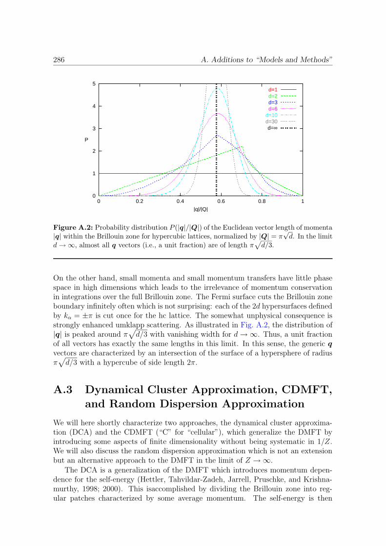
286 A. Additions to “Models and Methods”
0
1
2
3
4
5
0 0.2 0.4 0.6 0.8 1
P
|q|/|Q|
d=1d=2d=3d=6
d=10d=30d=∞
Figure A.2: Probability distribution P (|q|/|Q|) of the Euclidean vector length of momenta|q| within the Brillouin zone for hypercubic lattices, normalized by |Q| = π
√d. In the limit
d→∞, almost all q vectors (i.e., a unit fraction) are of length π√
d/3.
On the other hand, small momenta and small momentum transfers have little phasespace in high dimensions which leads to the irrelevance of momentum conservationin integrations over the full Brillouin zone. The Fermi surface cuts the Brillouin zoneboundary infinitely often which is not surprising: each of the 2d hypersurfaces definedby kα = ±π is cut once for the hc lattice. The somewhat unphysical consequence isstrongly enhanced umklapp scattering. As illustrated in Fig. A.2, the distribution of|q| is peaked around π
√
d/3 with vanishing width for d→∞. Thus, a unit fractionof all vectors has exactly the same lengths in this limit. In this sense, the generic qvectors are characterized by an intersection of the surface of a hypersphere of radiusπ√
d/3 with a hypercube of side length 2π.
A.3 Dynamical Cluster Approximation, CDMFT,
and Random Dispersion Approximation
We will here shortly characterize two approaches, the dynamical cluster approxima-tion (DCA) and the CDMFT (“C” for “cellular”), which generalize the DMFT byintroducing some aspects of finite dimensionality without being systematic in 1/Z.We will also discuss the random dispersion approximation which is not an extensionbut an alternative approach to the DMFT in the limit of Z →∞.
The DCA is a generalization of the DMFT which introduces momentum depen-dence for the self-energy (Hettler, Tahvildar-Zadeh, Jarrell, Pruschke, and Krishna-murthy, 1998; 2000). This isaccomplished by dividing the Brillouin zone into reg-ular patches characterized by some average momentum. The self-energy is then
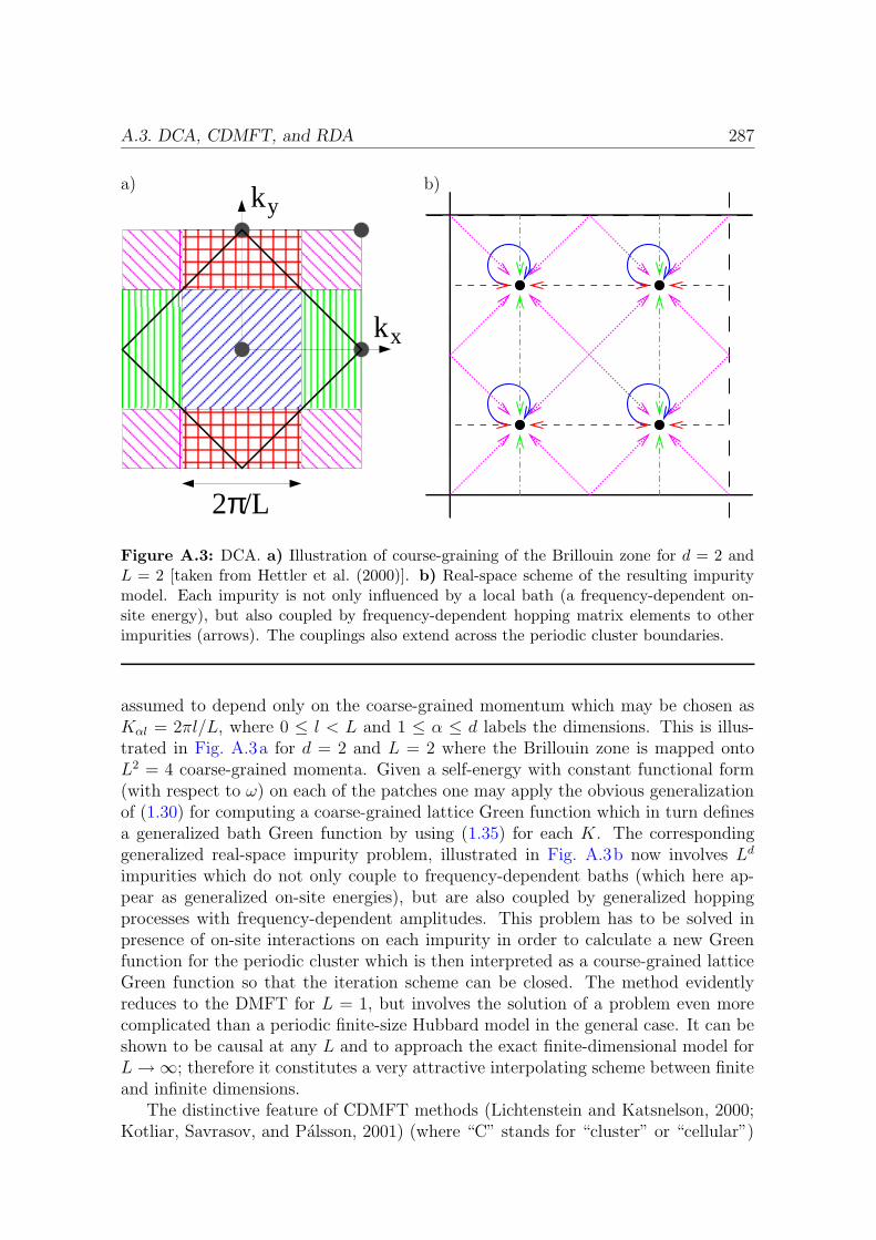
A.3. DCA, CDMFT, and RDA 287
a) b)
2π/L
kx
ky
Figure A.3: DCA. a) Illustration of course-graining of the Brillouin zone for d = 2 andL = 2 [taken from Hettler et al. (2000)]. b) Real-space scheme of the resulting impuritymodel. Each impurity is not only influenced by a local bath (a frequency-dependent on-site energy), but also coupled by frequency-dependent hopping matrix elements to otherimpurities (arrows). The couplings also extend across the periodic cluster boundaries.
assumed to depend only on the coarse-grained momentum which may be chosen asKαl = 2πl/L, where 0 ≤ l < L and 1 ≤ α ≤ d labels the dimensions. This is illus-trated in Fig. A.3a for d = 2 and L = 2 where the Brillouin zone is mapped ontoL2 = 4 coarse-grained momenta. Given a self-energy with constant functional form(with respect to ω) on each of the patches one may apply the obvious generalizationof (1.30) for computing a coarse-grained lattice Green function which in turn definesa generalized bath Green function by using (1.35) for each K. The correspondinggeneralized real-space impurity problem, illustrated in Fig. A.3b now involves Ld
impurities which do not only couple to frequency-dependent baths (which here ap-pear as generalized on-site energies), but are also coupled by generalized hoppingprocesses with frequency-dependent amplitudes. This problem has to be solved inpresence of on-site interactions on each impurity in order to calculate a new Greenfunction for the periodic cluster which is then interpreted as a course-grained latticeGreen function so that the iteration scheme can be closed. The method evidentlyreduces to the DMFT for L = 1, but involves the solution of a problem even morecomplicated than a periodic finite-size Hubbard model in the general case. It can beshown to be causal at any L and to approach the exact finite-dimensional model forL→∞; therefore it constitutes a very attractive interpolating scheme between finiteand infinite dimensions.
The distinctive feature of CDMFT methods (Lichtenstein and Katsnelson, 2000;Kotliar, Savrasov, and Palsson, 2001) (where “C” stands for “cluster” or “cellular”)

288 A. Additions to “Models and Methods”
DMFTQMC
T(K)
d-SC
PG
AF
M
100
200
300
0.6
0.4
0.02
0.04
F(0)
0.2
0.2x
Bµ(
0.10.0 0.4
0
)
(b)
(c)
Figure A.4: CDMFT: the lattice is broken up in clusters (here with 2x2 sites); one of theseis treated explicitly (e.g., using QMC) while the influence of the others is captured in acavity picture analogous to the DMFT (scheme adapted from Lichtenstein and Katsnelson(2000)).
is the direct formulation in real (not momentum) space. Here, the lattice is dividedup into free finite-size clusters, one of which is treated explicitly and embedded into amedium which gives a mean-field estimate of the effect of the surrounding clusters asillustrated in Fig. A.4. In contrast to the DCA, the cluster is here free, i.e., does nothave periodic boundary conditions. Consequently, the analogue of (1.35) cannot beformulated in momentum space, but involves explicit matrix inversions in the clusterindices. Again, one can show causality and the interpolating character towards finitedimensions.
At least conceptionally, one should expect the CDMFT methods to yield a betterdescription for short-range correlations within the first few nearest-neighbor shellsthan the DCA since here the cluster Hamiltonian is in direct correspondence to thelattice Hamiltonian. On the other hand, CDMFT breaks the lattice translationalsymmetry6 which is preserved in DCA so that the DCA should give a better overallmomentum resolution for the same number of cluster sites (and L > 2). First resultsfor the d = 2 Hubbard model show that the nonlocal extensions of the DMFT indeedintroduce d-wave type superconducting correlations (Lichtenstein and Katsnelson,2000; Maier, Jarrell, Pruschke, and Keller, 2000). Very recently, finite-size effectswere found to be smaller for the DCA treatment in a comparative study (Maier andJarrell, 2002). For a detailed pedagogical review of the DCA method, see Jarrell,Maier, Hettler, and Tahvildarzadeh (2001).
The random-dispersion approximation (RDA) is not an extension, but an alter-native to the DMFT approach. It avoids the self-consistency cycle inherent in all
6Since edge sites of the CDMFT cluster have a reduced number of direct hopping bonds, they arerelatively stronger coupled to the effective medium and can, thus, be expected to be more mean-fieldlike than inner sites. This is opposite to a direct calculation on a finite cluster with open boundaryconditions where edge sites have less mean-field character.

A.3. DCA, CDMFT, and RDA 289
solutions of the DMFT (and its extensions mentioned above). Instead, it is basedon the factorization of the noninteracting 2-particle density of states (1.24), whichis assumed to apply to all momenta except for q = 0 and, where appropriate, forq = Q. Such a system can in principle be obtained for a given DOS as follows(Gebhard, 1997): for a finite system, one randomly assigns the kinetic energy εk toeach k point in the Brillouin zone where the probability P (ε) of finding the energyεk in the semi-open interval [ε − ∆ε/2, ε + ∆ε/2[ is given in terms of the DOS byP (ε) = ρ(ε)∆ε. In practice, one usually starts with a smooth dispersion and ap-plies a random permutation to the momenta, so that the dispersion is again random,but the DOS of each realization exactly equals the (discretized) target DOS. Sincethe randomization destroys the topology of the lattice anyway, the method can beformally applied in any dimension; for large enough systems it is claimed to be self-averaging. Due to the neglect of correlations in the noninteracting 2-particle DOS,the RDA makes a large error for processes with small momentum transfer, even inlarge dimensions (cf. the discussion in subsection 1.2.2) which might affect thermo-dynamic properties although the associated phase space becomes vanishingly small.Still, it is not apparent how this should be a source of the large discrepancies be-tween RDA estimates for the paramagnetic metal-insulator transition (Noack andGebhard, 1999) in comparison to all recent DMFT estimates (see chapter 3). Upto now, numerical results for the RDA have suffered from considerable finite-size ef-fects, since the number of k points was restricted to a value of 14 or smaller so farin an exact diagonalization scheme. Reliable evaluation methods for bigger systemsare needed for the RDA problem, e.g., an efficient formulation of the density matrixrenormalization group (DMRG) method (White, 1992; 1993) in k-space, in order toclarify if the different transition scenario is a genuine property of the RDA theory.

290 A. Additions to “Models and Methods”
291
Appendix B
Hyperdiamond Lattice
The hyperdiamond (hd) lattice is a bipartite non-Bravais lattice which generalizes thed = 2 honeycomb lattice and the d = 3 diamond lattice to arbitrary dimensions. Inaddition to the usual definition and recursive construction (Santoro, Airoldi, Sorella,and Tosatti, 1993) we will here use a representation in d + 1 dimensions (van Don-gen, 1997). As we will show, only the latter clearly exposes the isotropy of the hy-perdiamond lattice in the long-wavelength limit and allows for a computation of theoptical conductivity not only in d =∞ but, within the local approximation for self-energy Σ and particle-hole irreducible vertex Γ, also for arbitrary finite dimensions(see chapter 4). Although an extension to longer range hopping is straightforwardwe will in this section only consider NN hopping.
A general characterization of the hyperdiamond lattice in dimension d ≥ 1 is(Santoro et al., 1993)
1. each lattice site has d+ 1 nearest neighbors (NN),
2. the angle between each pair of d+1 unit1 primitive lattice vectors τ l connectinga site to its NN is constant,
τ l · τm = γd, (B.1)
3. for d > 1, there is no site-centered inversion symmetry, but only bond-centeredinversion symmetry,
where the last statement follows from the first two. The lack of inversion symmetryimplies that the unit vectors τ l cannot be the same on A and B sublattices. Insteadthey are related by an inversion operation, τB
l = −τAl . Thus it is useful to rewritethe noninteracting Hamiltonian by explicitly separating A and B lattice sites,
H0 = −t∑
〈i,j〉,σ
(
c†riσcrjσ
+ c†riσcrjσ
)
= −t∑
i∈A,σ
∑
l
c†ri+τA
l,σcriσ− t
∑
j∈B,σ
∑
l
c†rj+τB
l,σcrjσ
= −t[ ∑
i∈A,σ
∑
l
c†ri+τ l,σcriσ
+∑
j∈B,σ
∑
l
c†rj−τ l,σcrjσ
]
, (B.2)
1As usual, we define the lattice spacing such that NNs have unit distance.

292 B. Hyperdiamond Lattice
where 〈i, j〉 denotes NN hopping bonds and τ l ≡ τAl .For the hyperdiamond lattice (hd), these hopping vectors can be constructed
recursively:
1. start with a regular chain,
τ 1 = (1), τ 2 = (−1) for d = 1 (B.3)
2. given a set τ ′l of primitive lattice vectors in dimension d− 1, define
τ l =
(√
1− γ2dτ
′l, γd), l = 1, 2, . . . , d
(0, 0, . . . , 0, 1)︸ ︷︷ ︸
d components
, l = d+ 1 (B.4)
γd =γd−1
1− γd−1
= −1
d. (B.5)
Now, the noninteracting tight-binding Hamiltonian (with NN hopping) in Fouriertransformed form remains offdiagonal in the sublattice index α ∈ A,B,
H0 =
(0 H1
H∗1 0
)
, H1 = −td+1∑
m=1
e−ik·τm , (B.6)
where the eigenvalues form two energy bands εnk = ±|H1|. This expression can besimplified by a transformation in momentum space (α = 1, . . . , d),
k′α =∑
β
Aαβkβ, Aαβ = (aα)β, aα = τ d+1 − τα . (B.7)
Eliminating an overall phase factor e−ik·τd+1 we have
εnk = ±t∣∣∣1 +
d∑
α=1
eik′α
∣∣∣, −π ≤ k′α ≤ π, (B.8)
which provides a convenient way to compute the DOS and shows that perfect nestingis not possible on the bipartite hd lattice. In the limit d → ∞, where the hoppingamplitude has to be scaled as t = t∗/(d+1), the DOS is readily evaluated analytically,
ρhd(ε) =|ε|t∗2
e−ε2/t∗2
. (B.9)
Calculations of properties which directly depend on k (i.e., not only via εnk), inparticular transport properties, however, require knowledge of the transformationmatrix (Aαβ). As a general example for this problem let us consider the Fermivelocity vk = −∇εk for an energy function defined in terms of transformed k vectors,εk = f(Ck) with arbitrary function f and matrix C. In the present case, where
293
the functional form of f is explicitly known, one can first compute the derivativev′k′ = −∇k′f(k′) and then apply the transformation
∂f(Ck)
∂kα=
∑
β
∂f
∂k′β
∂(Ck)β∂kα
=∑
β
Aβα∂f
∂k′β(B.10)
vk = CTv′k′
∣∣k′=Ck
. (B.11)
While the transformation matrix defined via (B.3)-(B.5) and (B.7) can be evaluatedin any finite dimension, this is in general a complicated task and it is unclear howto take the limit d → ∞ of (B.10). Furthermore, symmetries are hidden so that itis not even apparent if observables which transform like a tensor such as, e.g., theoptical conductivity will be isotropic in all dimensions.
Thus, we switch to an alternative representation of the hyperdiamond latticewhich embeds the d-dimensional hd lattice into d+1 host dimensions in the followingway (van Dongen, 1997): starting with a d + 1-dimensional hypercube with NNhopping we remove every second bond such that the unit vectors connecting to NNsare for sublattices A and B
τAl = el, τBl = −el . (B.12)
Here, el are the usual cartesic unit vectors in d + 1 dimensions; the tilde (∼)indicates properties in the expanded d + 1-dimensional vector space. For sake ofdefiniteness we define the origin to belong to the A sublattice. Figure B.1 illustratesthis embedding for d = 2, i.e., the honeycomb lattice.
It is clear from (B.2) that a tight-binding Hamiltonian defined on a periodiclattice with fixed uniform NN hopping is fully defined by the topology of the hoppingbonds and invariant under distortions. Since the lattice defined by (B.12) has d + 1NN bonds with a constant angle (here: π/2) between each pair of them, it (moreprecisely: each sheet of sites connected by hopping bonds) is indeed topologicallyequivalent to the usual hyperdiamond lattice and has both the same noninteractingDOS and the same single-particle properties for arbitrary additional local interaction.The noninteracting dispersion is given by
εk = ±1
2
√
(εhck
)2 + ε2k, (B.13)
where εhck
= −2t∑d+1
l=1 cos(kl) and εk = 2t∑d+1
l=1 sin(kl). Again, one of the kl couldbe singled out and be fixed for calculations of the DOS, exposing the equivalence ofthe dispersions (B.8) and (B.13). Since 〈(εhc
k)2〉 = 〈ε2
k〉 = 2(d + 1)t2, we can read
off from (B.13) that the variance of the DOS of the hyperdiamond lattice is exactly(d + 1)t2 = t∗2 in any dimension. Note, however, that in the present derivation kremains untransformed within the (halved) Brillouin zone which allows for a directcalculation of the Fermi velocity (in d+ 1 dimensions),
(vk)l =t
εk
(
εhck
sin(kl) + εk cos(kl))
. (B.14)
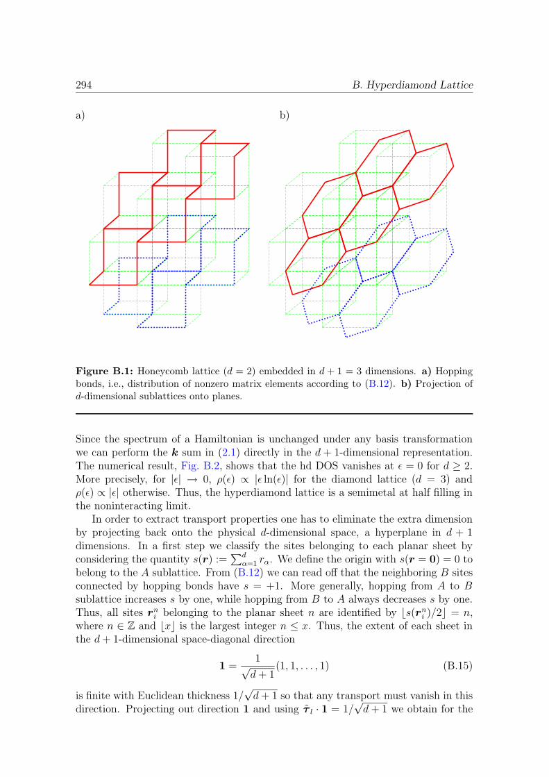
294 B. Hyperdiamond Lattice
a) b)
Figure B.1: Honeycomb lattice (d = 2) embedded in d + 1 = 3 dimensions. a) Hoppingbonds, i.e., distribution of nonzero matrix elements according to (B.12). b) Projection ofd-dimensional sublattices onto planes.
Since the spectrum of a Hamiltonian is unchanged under any basis transformationwe can perform the k sum in (2.1) directly in the d + 1-dimensional representation.The numerical result, Fig. B.2, shows that the hd DOS vanishes at ε = 0 for d ≥ 2.More precisely, for |ε| → 0, ρ(ε) ∝ |ε ln(ε)| for the diamond lattice (d = 3) andρ(ε) ∝ |ε| otherwise. Thus, the hyperdiamond lattice is a semimetal at half filling inthe noninteracting limit.
In order to extract transport properties one has to eliminate the extra dimensionby projecting back onto the physical d-dimensional space, a hyperplane in d + 1dimensions. In a first step we classify the sites belonging to each planar sheet byconsidering the quantity s(r) :=
∑dα=1 rα. We define the origin with s(r = 0) = 0 to
belong to the A sublattice. From (B.12) we can read off that the neighboring B sitesconnected by hopping bonds have s = +1. More generally, hopping from A to Bsublattice increases s by one, while hopping from B to A always decreases s by one.Thus, all sites rni belonging to the planar sheet n are identified by bs(rni )/2c = n,where n ∈ Z and bxc is the largest integer n ≤ x. Thus, the extent of each sheet inthe d+ 1-dimensional space-diagonal direction
1 =1√d+ 1
(1, 1, . . . , 1) (B.15)
is finite with Euclidean thickness 1/√d+ 1 so that any transport must vanish in this
direction. Projecting out direction 1 and using τ l · 1 = 1/√d+ 1 we obtain for the
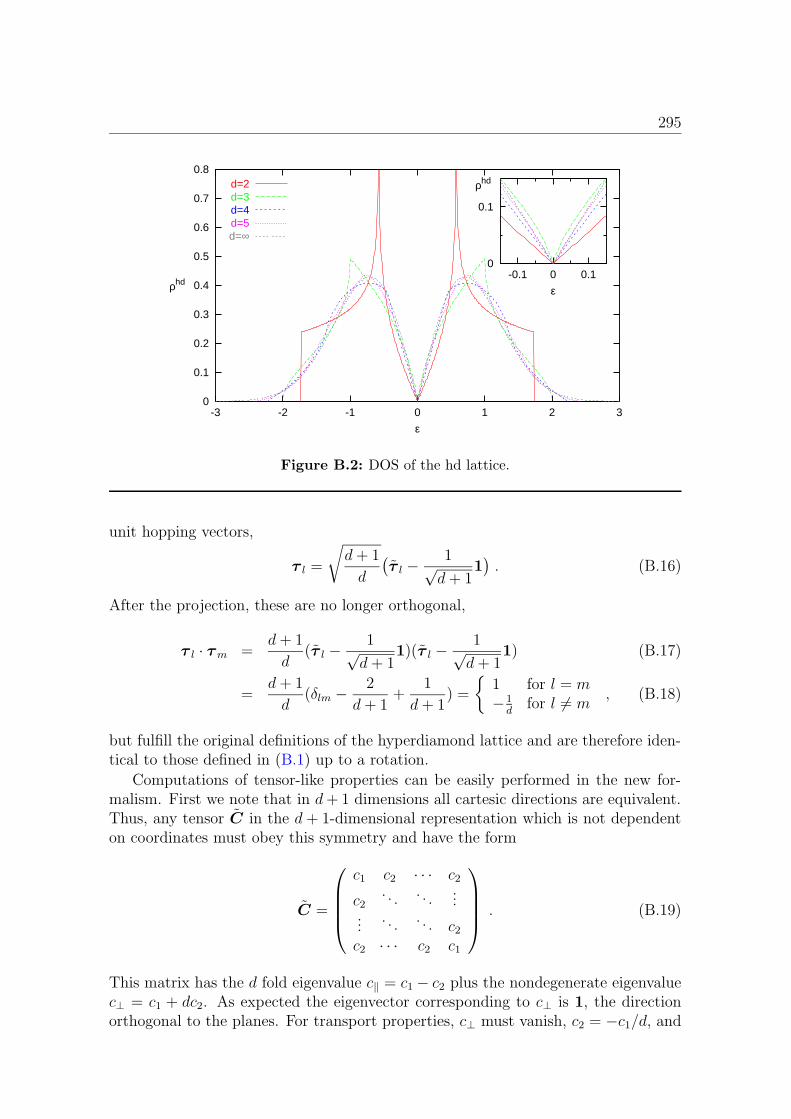
295
0
0.1
0.2
0.3
0.4
0.5
0.6
0.7
0.8
-3 -2 -1 0 1 2 3
ρhd
ε
d=2d=3d=4d=5d=∞
0
0.1
-0.1 0 0.1
ε
ρhd
Figure B.2: DOS of the hd lattice.
unit hopping vectors,
τ l =
√
d+ 1
d
(τ l −
1√d+ 1
1). (B.16)
After the projection, these are no longer orthogonal,
τ l · τm =d+ 1
d(τ l −
1√d+ 1
1)(τ l −1√d+ 1
1) (B.17)
=d+ 1
d(δlm −
2
d+ 1+
1
d+ 1) =
1 for l = m− 1d
for l 6= m, (B.18)
but fulfill the original definitions of the hyperdiamond lattice and are therefore iden-tical to those defined in (B.1) up to a rotation.
Computations of tensor-like properties can be easily performed in the new for-malism. First we note that in d+ 1 dimensions all cartesic directions are equivalent.Thus, any tensor C in the d + 1-dimensional representation which is not dependenton coordinates must obey this symmetry and have the form
C =
c1 c2 · · · c2
c2. . . . . .
......
. . . . . . c2c2 · · · c2 c1
. (B.19)
This matrix has the d fold eigenvalue c‖ = c1 − c2 plus the nondegenerate eigenvaluec⊥ = c1 + dc2. As expected the eigenvector corresponding to c⊥ is 1, the directionorthogonal to the planes. For transport properties, c⊥ must vanish, c2 = −c1/d, and
296 B. Hyperdiamond Lattice
we obtain
C = c1d+ 1
d
1 0 · · · 0
0. . . . . .
......
. . . . . . 00 · · · 0 1
. (B.20)
Thus, we have not only proven that transport properties are isotropic on the hyperdia-mond lattice in the long-wavelength limit2 for any dimension d, but also constructeda simple algorithm for the computation provided that the corresponding quantitycan be computed for the model in d+ 1 dimensions as defined by (B.12). Numericalresults for transport related quantities of the hd lattice can be found in subsection4.5.2.
2Note that for the honeycomb lattice the isotropy also follows from the simultaneous presenceof mirror symmetries x → −x, y → −y through the center of a bond in x or y direction and therotational symmetry (x, y)→ (x cos(2π/n) + y sin(2π/n)) with n > 2 (here n = 3).
297
Appendix C
Using Splines forFourier-TransformingImaginary-Time Green Functions
As discussed in subsection 3.4.1, the Fourier transformations of Green functions fromimaginary time to Matsubara frequencies and vice versa that arise in the QMC so-lution of the DMFT problem are not trivial. All problems can be traced back to thediscreteness of the QMC estimates Gl for time slices τl = l∆τ . However, the trueimaginary-time Green function G(τ) is known to be a smooth curve with continuousderivatives (of all orders) on the interval [0, β]. Thus, reasonable results can be ex-pected by performing the Fourier transform not for the discrete raw data, but for afitted smooth curve. In this appendix, we will give a short summary of work carriedout recently in collaboration with Knecht. More details can be found in Knecht’s(2002) diploma thesis and in upcoming publications.
The simplest practical approach in this context consists of a direct interpolationof the discrete QMC data by a cubic spline (with a continuous second derivative)as implemented by Krauth. While this step suffices for closing the self-consistencyequations without any further adjustments (like Ulmke’s smoothing trick), it leadsto nonanalytic behavior of the self-energy near and beyond the Nyquist frequency asillustrated in Fig. 3.11. In our view, this problem can be traced back to the fact thatthe natural spline chosen by Krauth is inadequate for this problem: By definition,the second derivative of a natural spline vanishes at its boundaries. However, all evenderivatives of the true Green function are maximal at the edges of the interval [0, β].The resulting misfit leads to unphysical ringing as illustrated in Fig. C.1. Here, thenoninteracting Green function for a semi-elliptic DOS is chosen as an example sinceit can be computed with arbitrary precision. Furthermore, moderate interactionsdo not lead to qualitative changes in the Green function so that the example isrepresentative. It is clearly seen that a fit of a discrete set of data points (here forΛ = 40 and β = 100, i.e., a large discretization ∆τ = 2.5) using a natural cubic splinewith continuous second derivative leads to a large error oscillating with the Nyquistfrequency. While the initial misfit at τ = 0 is similarly large for a natural Akimaspline, the oscillation decays significantly faster due to jumps in the second derivative
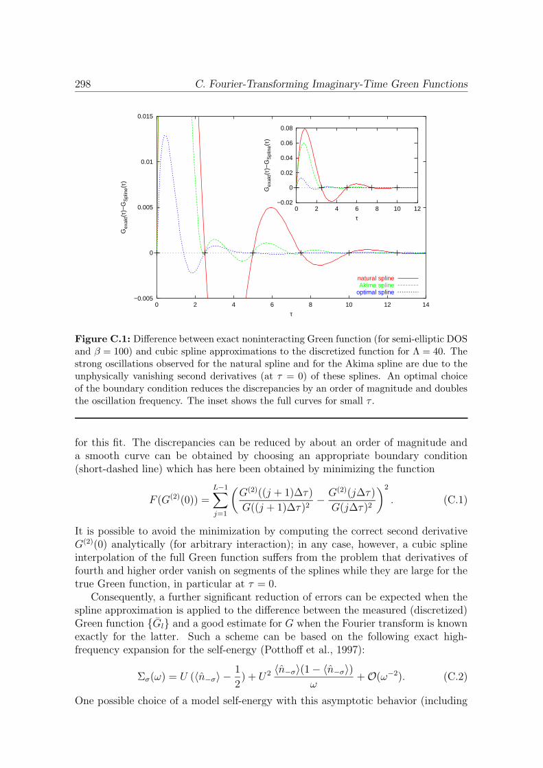
298 C. Fourier-Transforming Imaginary-Time Green Functions
−0.005
0
0.005
0.01
0.015
0 2 4 6 8 10 12 14
Gex
akt(τ
)−G
Spl
ine(
τ)
τ
natural splineAkima spline
optimal spline
−0.02
0
0.02
0.04
0.06
0.08
0 2 4 6 8 10 12
Gex
akt(τ
)−G
Spl
ine(
τ)
τ
Figure C.1: Difference between exact noninteracting Green function (for semi-elliptic DOSand β = 100) and cubic spline approximations to the discretized function for Λ = 40. Thestrong oscillations observed for the natural spline and for the Akima spline are due to theunphysically vanishing second derivatives (at τ = 0) of these splines. An optimal choiceof the boundary condition reduces the discrepancies by an order of magnitude and doublesthe oscillation frequency. The inset shows the full curves for small τ .
for this fit. The discrepancies can be reduced by about an order of magnitude anda smooth curve can be obtained by choosing an appropriate boundary condition(short-dashed line) which has here been obtained by minimizing the function
F (G(2)(0)) =L−1∑
j=1
(G(2)((j + 1)∆τ)
G((j + 1)∆τ)2− G(2)(j∆τ)
G(j∆τ)2
)2
. (C.1)
It is possible to avoid the minimization by computing the correct second derivativeG(2)(0) analytically (for arbitrary interaction); in any case, however, a cubic splineinterpolation of the full Green function suffers from the problem that derivatives offourth and higher order vanish on segments of the splines while they are large for thetrue Green function, in particular at τ = 0.
Consequently, a further significant reduction of errors can be expected when thespline approximation is applied to the difference between the measured (discretized)Green function Gl and a good estimate for G when the Fourier transform is knownexactly for the latter. Such a scheme can be based on the following exact high-frequency expansion for the self-energy (Potthoff et al., 1997):
Σσ(ω) = U (〈n−σ〉 −1
2) + U 2 〈n−σ〉(1− 〈n−σ〉)
ω+O(ω−2). (C.2)
One possible choice of a model self-energy with this asymptotic behavior (including

299
the ω−1 term) which is nonsingular (and purely imaginary) on the imaginary axis isgiven by
Σmodel,σ(ω) = U (〈n−σ〉 −1
2) +
1
2U2 〈n−σ〉
(1− 〈n−σ〉
)( 1
ω + ω0
+1
ω − ω0
). (C.3)
While the quality of the low-frequency part of this fit could be tuned by adjusting theparameter ω0, the value of this parameter is irrelevant for the following as long as itis not much larger than the bandwidth; we will choose ω0 = 1. By evaluating Σmodel
on the imaginary axis, the corresponding Green function Gmodel can be computed foran arbitrary number of Matsubara frequencies. Consequently, the Fourier transfor-mation to imaginary time is unproblematic (when the “free” term 1/(iωn) is takencare of analytically). Thus, the difference of the Green functions can be accuratelyevaluated at all time slices. Since the second derivative of the transformed modelGreen function at τ = 0 exactly reproduces that of the true Green function, thedifference is well represented by a natural spline. The Green function is obtained asa function of Matsubara frequencies by Fourier transforming the oversampled splineand adding the Matsubara-frequency model Green function to the result.
Predictions for the imaginary-time self-energy of the half-filled Hubbard modelwith semi-elliptic DOS at T = 0.1 resulting from the scheme described above fora range of discretizations 0.1 ≤ ∆τ ≤ 0.4 are shown in Fig. C.2 for the correlatedmetallic phase at U = 4.0 and in Fig. C.3 for the insulating phase at U = 5.0.All results show the correct asymptotic behavior at large frequencies. Oscillatorybehavior which is initially observed at intermediate frequencies (see insets) becomesundetectable for ∆τ . 0.2 in both figures. The convergence at small frequencies isgood; it will be further discussed below.
One fundamental difference of the QMC code previously used in our group (basedon Ulmke’s smoothing trick, cf. subsection 3.4.1) is that it does not make predictionsfor the self-energy beyond the Nyquist frequency as seen in Fig. C.4 and Fig. C.5.Even worse, the ∆τ error is also large at intermediate and small frequencies. In fact,the insulating solutions are even qualitatively wrong at small frequencies for largevalues of ∆τ .
In contrast, the results of the improved QMC method developed within this the-sis and used throughout chapter 3 depicted in Fig. C.6 and Fig. C.7 show goodconvergence in the most important small-frequency region. In fact, the ∆τ error isasymptotically almost identical to that of the new optimal scheme at small frequen-cies, at least in the range ∆τ ≤ 0.25 used within this thesis.
This is also seen in Fig. C.8, where the Eliashberg estimate of the quasiparticleweight Z (cf. subsection 3.2.3) is shown as a function of ∆τ 2. Both in the metallicand in the insulating phase, the new approach yields the smallest errors which arenearly perfectly quadratic in ∆τ . The systematic errors of the QMC program used inchapter 3 are identical (within statistical errors) at small ∆τ and only slightly largerfor ∆τ & 0.25. In contrast, Ulmke’s method leads to ∆τ errors which are larger bya full order of magnitude in the insulating case.
While these results of Knecht’s (2002) thesis reproduced in this appendix confirmthat the QMC code used in chapter 3 is indeed adequate for studies of the Mott
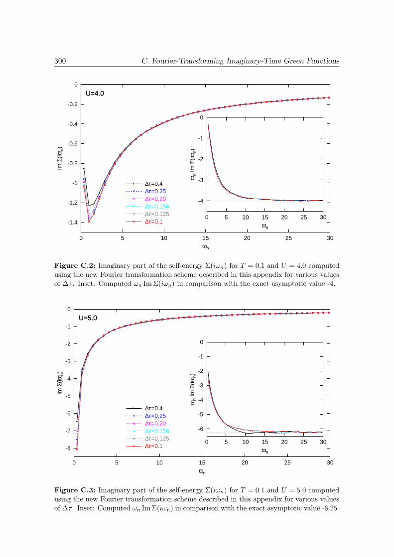
300 C. Fourier-Transforming Imaginary-Time Green Functions
-1.4
-1.2
-1
-0.8
-0.6
-0.4
-0.2
0
0 5 10 15 20 25 30
Im Σ
(iωn)
ωn
U=4.0
∆τ=0.4∆τ=0.25∆τ=0.20∆τ=0.156∆τ=0.125∆τ=0.1
-4
-3
-2
-1
0
0 5 10 15 20 25 30
ωn
Im Σ
(iωn)
ωn
U=4.0
Figure C.2: Imaginary part of the self-energy Σ(iωn) for T = 0.1 and U = 4.0 computedusing the new Fourier transformation scheme described in this appendix for various valuesof ∆τ . Inset: Computed ωn Im Σ(iωn) in comparison with the exact asymptotic value -4.
-8
-7
-6
-5
-4
-3
-2
-1
0
0 5 10 15 20 25 30
Im Σ
(iωn)
ωn
U=5.0
∆τ=0.4∆τ=0.25∆τ=0.20∆τ=0.156∆τ=0.125∆τ=0.1
-6
-5
-4
-3
-2
-1
0
0 5 10 15 20 25 30
ωn
Im Σ
(iωn)
ωn
U=5.0
Figure C.3: Imaginary part of the self-energy Σ(iωn) for T = 0.1 and U = 5.0 computedusing the new Fourier transformation scheme described in this appendix for various valuesof ∆τ . Inset: Computed ωn Im Σ(iωn) in comparison with the exact asymptotic value -6.25.
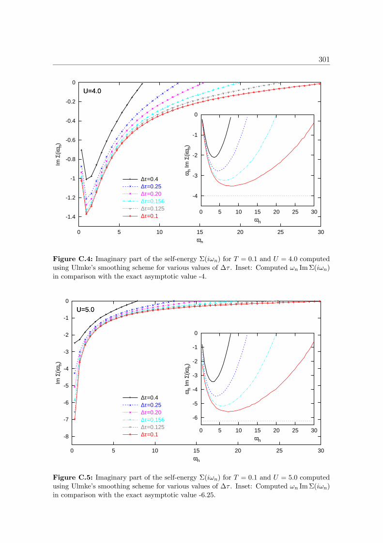
301
-1.4
-1.2
-1
-0.8
-0.6
-0.4
-0.2
0
0 5 10 15 20 25 30
Im Σ
(iωn)
ωn
U=4.0
∆τ=0.4∆τ=0.25∆τ=0.20∆τ=0.156∆τ=0.125∆τ=0.1
-4
-3
-2
-1
0
0 5 10 15 20 25 30
ωn
Im Σ
(iωn)
ωn
U=4.0
Figure C.4: Imaginary part of the self-energy Σ(iωn) for T = 0.1 and U = 4.0 computedusing Ulmke’s smoothing scheme for various values of ∆τ . Inset: Computed ωn Im Σ(iωn)in comparison with the exact asymptotic value -4.
-8
-7
-6
-5
-4
-3
-2
-1
0
0 5 10 15 20 25 30
Im Σ
(iωn)
ωn
U=5.0
∆τ=0.4∆τ=0.25∆τ=0.20∆τ=0.156∆τ=0.125∆τ=0.1
-6
-5
-4
-3
-2
-1
0
0 5 10 15 20 25 30
ωn
Im Σ
(iωn)
ωn
U=5.0
Figure C.5: Imaginary part of the self-energy Σ(iωn) for T = 0.1 and U = 5.0 computedusing Ulmke’s smoothing scheme for various values of ∆τ . Inset: Computed ωn Im Σ(iωn)in comparison with the exact asymptotic value -6.25.

302 C. Fourier-Transforming Imaginary-Time Green Functions
-1.4
-1.2
-1
-0.8
-0.6
-0.4
-0.2
0
0 5 10 15 20 25 30
Im Σ
(iωn)
ωn
U=4.0
∆τ=0.4∆τ=0.25∆τ=0.20∆τ=0.156∆τ=0.125∆τ=0.1
-4
-3
-2
-1
0
0 5 10 15 20 25 30
ωn
Im Σ
(iωn)
ωn
U=4.0
Figure C.6: Imaginary part of the self-energy Σ(iωn) for T = 0.1 and U = 4.0 resultingfrom the QMC code used throughout chapter 3 for various values of ∆τ . Inset: Computedωn Im Σ(iωn) in comparison with the exact asymptotic value -4.
-8
-7
-6
-5
-4
-3
-2
-1
0
0 5 10 15 20 25 30
Im Σ
(iωn)
ωn
U=5.0
∆τ=0.4∆τ=0.25∆τ=0.20∆τ=0.156∆τ=0.125∆τ=0.1
-6
-5
-4
-3
-2
-1
0
0 5 10 15 20 25 30
ωn
Im Σ
(iωn)
ωn
U=5.0
Figure C.7: Imaginary part of the self-energy Σ(iωn) for T = 0.1 and U = 5.0 resultingfrom the QMC code used throughout chapter 3 for various values of ∆τ . Inset: Computedωn Im Σ(iωn) in comparison with the exact asymptotic value -6.25.
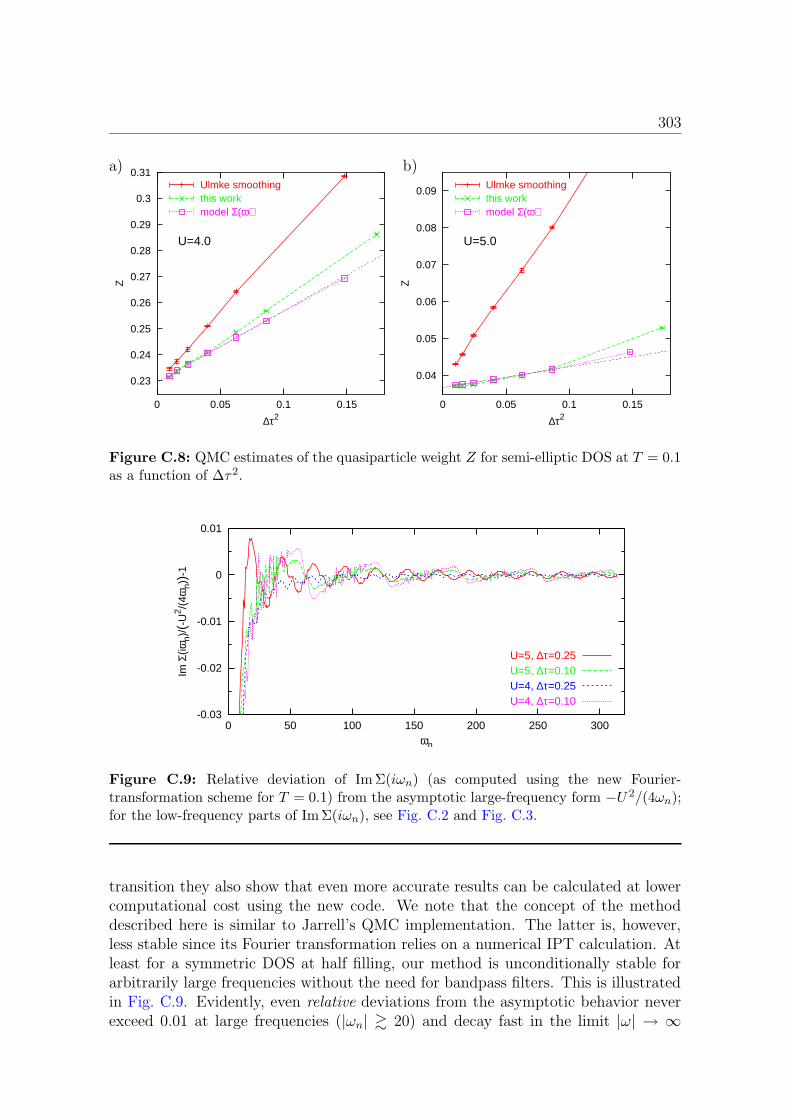
303
a) b)
0.23
0.24
0.25
0.26
0.27
0.28
0.29
0.3
0.31
0 0.05 0.1 0.15
Z
∆τ2
U=4.0
Ulmke smoothingthis workmodel Σ(ω)
0.04
0.05
0.06
0.07
0.08
0.09
0 0.05 0.1 0.15Z
∆τ2
U=5.0
Ulmke smoothingthis workmodel Σ(ω)
Figure C.8: QMC estimates of the quasiparticle weight Z for semi-elliptic DOS at T = 0.1as a function of ∆τ 2.
-0.03
-0.02
-0.01
0
0.01
0 50 100 150 200 250 300
Im Σ
(iωn)
/(-U
2 /(4ω
n))-
1
ωn
U=5, ∆τ=0.25U=5, ∆τ=0.10U=4, ∆τ=0.25U=4, ∆τ=0.10
Figure C.9: Relative deviation of Im Σ(iωn) (as computed using the new Fourier-transformation scheme for T = 0.1) from the asymptotic large-frequency form −U 2/(4ωn);for the low-frequency parts of Im Σ(iωn), see Fig. C.2 and Fig. C.3.
transition they also show that even more accurate results can be calculated at lowercomputational cost using the new code. We note that the concept of the methoddescribed here is similar to Jarrell’s QMC implementation. The latter is, however,less stable since its Fourier transformation relies on a numerical IPT calculation. Atleast for a symmetric DOS at half filling, our method is unconditionally stable forarbitrarily large frequencies without the need for bandpass filters. This is illustratedin Fig. C.9. Evidently, even relative deviations from the asymptotic behavior neverexceed 0.01 at large frequencies (|ωn| & 20) and decay fast in the limit |ω| → ∞
304 C. Fourier-Transforming Imaginary-Time Green Functions
which is here cut off by the (constant) number of 1000 Matsubara frequencies usedin the QMC program. Note that the large deviations from the asymptotic behaviorat relatively low frequencies are physical; indeed, these deviations are the nontrivialresult of the QMC calculations.
For further practical applications of the new QMC code and for the generalizationof the asymptotic expansion of the self-energy to the multi-band case, see Knecht(2002). Interestingly, the multi-band case is more complicated: here, the expansionof the self energy does not only involve expectation values of densities, but also ofpairwise double occupancies.
305
Appendix D
Linear Response toElectromagnetic Fields
In this appendix, we review the formalism necessary for identifying the quantizedHamiltonian for particles in an electromagnetic field and give a short summary oflinear-response theory.
D.1 Electromagnetic Interaction Hamiltonian and
Choice of Gauge
Classically, the equation of motion for a nonrelativistic particle with charge q andmomentum mv at position r in an external electromagnetic field is1
mr = qE(r, t) +q
cr ×B(r, t), (D.1)
where the right hand side is the Lorentz force. The electric field E and the magneticfield B can be expressed in terms of a vector potential A and a scalar potential φ,
B(r, t) = ∇×A(r, t); E(r, t) = −∇φ(r, t)− 1
c
∂A(r, t)
∂t. (D.2)
A generalization for quantum systems is best derived via the manifestly Lorentzinvariant action which for a world line beginning at a = (ct1, r2) and ending atb = (ct2, r2) reads [see, e.g., Landau and Lifschitz (1992)]
S =
b∫
a
(−mc2 dτ −∑
α
q
cAα dxα), (D.3)
Here, dτ = dt/γ, where γ−1 =√
1− (v/c)2; xα = (ct, r) and Aα = (φ,A) are 4-vectors. Rewriting (D.3) in terms of a time integral we can identify the Lagrangian
1Here, we use the cgs system. All equations may be transformed into the SI system by multiplyingB, A, and Aα by the speed of light, c.
306 D. Linear Response to Electromagnetic Fields
(v = r),
L = −mc2√
1− v2
c2+q
cA · v − qφ. (D.4)
Expressing the Hamiltonian,
H = v · ∂L∂v− L =
mc2√
1− v2
c2
+ qφ, (D.5)
in terms of the canonical momentum p (component-wise derivative),
p =∂L∂v
=mv
√
1− v2
c2
+q
cA (D.6)
one arrives at the final relativistic expression,
H(p, r, t) =
√
m2c4 + c2(
p− q
cA(r, t)
)2
+ qφ(r, t) (D.7)
≈ mc2(
1 +1
2
(p− ecA(r, t)
mc
)2
− 1
4
(p− ecA(r, t)
mc
)4)
+ qφ(r, t) . (D.8)
In the nonrelativistic limit, only the leading nonconstant term needs to be kept,
H(p, r, t) ≈ H +1
2m
(
p− q
cA(r, t)
)2
+ qφ(r, t). (D.9)
The Lorentz force given in (D.1) is easily reproduced from the corresponding La-grangian.
The potentials A, φ are not uniquely defined by the physical fields E, B; thelatter remain unchanged under a gauge transformation
A(r, t) −→ A′(r, t) = A(r, t) +∇χ(r, t) (D.10)
φ(r, t) −→ φ′(r, t) = φ(r, t)− 1
c
∂χ(r, t)
∂t. (D.11)
The Coulomb gauge ∇ ·A = 0 (also called transverse gauge) is particularly suitablefor the study of interacting electron systems, because φ acts instantaneously in thiscase. An oscillatory electric field is then represented by the field A only. Note thatthis treatment implies an infinitely growing vector potential in the limit ω → 0 whichat least a priori gives reason for caution in connection with linear response theory.The final expressions for the dc conductivity can, however, also be computed directlywith the same result (Luttinger, 1964; Mahan, 1990).
D.2 Linear Response Theory
Let a system be subjected to a time-dependent perturbation F (t) which couplesthrough an operator A,
H(t) = H0 + H1(t) = H0 − AF (t) . (D.12)
D.2. Linear Response Theory 307
We assume that the function is switched on adiabatically,
F (t)t→−∞−→ 0;
∣∣d
dtF (t)
∣∣ <∞ . (D.13)
Then, the evolution of the density operator for an ensemble of perturbed systems atfinite temperature from the unperturbed density operator,
ρ0 =1
Z0
e−βH0 , Z0 = Tre−βH0
=∑
n
e−βEn , (D.14)
is determined by the von Neumann equation,
ρ(t = −∞) = ρ0; i~d
dtρ(t) = [H(t), ρ(t)] . (D.15)
Due to the invariance of the trace with respect to cyclical permutations, expecta-tion values of operators may be equivalently expressed in the Schrodinger or in theinteraction picture,
〈B〉F := TrB ρ(t)
= Tr
BI(t) ρI(t)
. (D.16)
Here, we denote expectation values in the perturbed ensemble as 〈. . . 〉F and operators
in the interaction picture as XI(t) := eiH0t/~Xe−iH0t/~. The corresponding equationof motion for the density operator plus the initial condition are equivalent to theintegral equation
ρI(t) = ρ0 +i
~
t∫
−∞
dt′ [AI(t′), ρI(t
′)]F (t′) , (D.17)
which may be solved iteratively. Inserting the unperturbed density operator in theright hand side of (D.17) yields the lowest order (i.e., linear) correction. UsingTrBI(t)[AI(t), ρ0]
= Tr
ρ0[BI(t), AI(t)]
one, thus, obtains to linear order
〈B〉F (t) = 〈B〉0 +
∞∫
−∞
dt′ F (t′)χB,A(t, t′) , (D.18)
with the retarded susceptibility
χB,A(t, t′) =i
~〈[BI(t), AI(t
′)]〉0Θ(t− t′) . (D.19)
Specializing on harmonic time dependence of the perturbation,
F (t) = F0e−i(ω+iδ)t, (D.20)
one can also derive the formulation in frequency space,
〈B〉F (ω) = 〈B〉0 + 〈〈B, A〉〉(ω + iδ)F (ω) (D.21)
308 D. Linear Response to Electromagnetic Fields
using the definition
〈〈B, A〉〉(ω + iδ) ≡ χB,A(ω + iδ) =i
~
∞∫
0
dt〈[BI(t), A]〉0 ei(ω+iδ)t . (D.22)
Performing the trace for an eigenbasis of the unperturbed Hamiltonian, inserting theidentity 1 =
∑
m |m〉〈m| between the operators, and reordering terms one obtainsthe (thermal) spectral representation,
〈〈B, A〉〉(ω + iδ) =i
~
1
Z0
∑
n,m
e−βEn
∞∫
0
dt(
eit(ω+iδ+ En−Em~
)〈n|B|m〉〈m|A|n〉
− eit(ω+iδ−En−Em~
)〈n|A|m〉〈m|B|n〉)
(D.23)
= − 1
Z0
∑
n,m
〈n|B|m〉〈m|A|n〉~(ω + iδ) + En − Em
(e−βEn − e−βEm
). (D.24)
If we further assume that the spectrum of H0 is bounded, we find from (D.24) forthe limiting behavior,
〈〈B, A〉〉(ω + iδ)ω→∞−→ − 1
~ω〈[B, A]〉0 +O
( 1
ω2
). (D.25)
For the usual case A = B the leading term in (D.25) vanishes so that the susceptibilityχB,B then falls off at least as 1/ω2. Finally, the imaginary part of the susceptibility
can be simplified when 〈n|B|m〉〈m|A|n〉 is real. In particular, one obtains for B = A†
(i.e., for B = A when A is hermitian),
Im 〈〈B†, B〉〉(ω) =π
~Z0
∑
n,m
∣∣〈m|B|n〉
∣∣2δ(ω +
En − Em~
)(e−βEn − e−βEm
)(D.26)
T→0−→ π
~
∑
m
∣∣〈m|B|0〉
∣∣2(δ(ω − Em − E0
~)− δ(ω +
Em − E0
~)).(D.27)

309
Bibliography
Abbate, M., F. M. F. de Groot, J. C. Fuggle, A. Fujimori, Y. Tokura, Y. Fujishima,O. Strebel, M. Domke, G. Kaindl, J. van Elp, B. T. Thole, G. A. Sawatzky, M.Sacchi, and N. Tsuda, 1991, Phys. Rev. B 44, 5419. 267, 268
Abramowitz, M., and I. A. Stegun, 1972, Handbook of Mathematical Functions(Dover, New York). 49
Abrikosov, A. A., and I. M. Khalatnikov, 1958, Sov. Phys. JETP 6, 888. 11
Ahn, K. H., and A. J. Millis, 2000, Phys. Rev. B 61, 13545. 272
Altarelli, M., D. L. Dexter, H. M. Nussenzveig, and D. Y. Smith, 1972, Phys. Rev.B 6, 4502. 178
Andersen, O. K., 1975, Phys. Rev. B 12, 3060. 251
Andersen, O. K., Z. Pawlowska, and O. Jepsen, 1986, Phys. Rev. B 34, 5253. 251,252
Anderson, P. W., 1961, Phys. Rev. 124, 41. 282
Anisimov, V. I., A. I. Poteryaev, M. A. Korotin, A. O. Anokhin, and G. Kotliar,1997, J. Phys. Cond. Matter 9, 7359. 253, 254, 255, 261
Anisimov, V. I., J. Zaanen, and O. K. Andersen, 1991, Phys. Rev. B 44, 943. 252
Ashcroft, N. W., and N. D. Mermin, 1976, Solid State Physics (Holt-Saunders,Philadelphia). 9
Baeriswyl, D., D. K. Campbell, J. M. P. Carmelo, F. Guinea, and E. Louis, 1995,The Hubbard Model: Its Physics and Mathematical Physics (Plenum Press, NewYork). 10
Bansil, A., and M. Lindroos, 1999, Phys. Rev. Lett. 83, 5154. 259
Bao, W., C. Broholm, G. Aeppli, P. Dai, J. M. Honig, and P. Metcalf, 1997, Phys.Rev. Lett. 78, 507. 68
Bao, W., C. Broholm, G. Aeppli, S. A. Carter, P. Dai, T. F. Rosenbaum, J. M. Honig,P. Metcalf, and S. F. Trevino, 1998, Phys. Rev. B 58, 12727. 68
310 Bibliography
Bao, W., C. Broholm, S. A. Carter, T. F. Rosenbaum, G. Aeppli, S. F. Trevino, P.Metcalf, J. M. Honig, and J. Spalek, 1993, Phys. Rev. Lett. 71, 766. 68
Batson, P. E., and J. Silcox, 1983, Phys. Rev. B 27, 5224. 183
Berlin, T. H., and M. Kac, 1952, Phys. Rev. 86, 821. 13
Bethe, H. A., 1930, Ann. Physik 5, 325. 179
Bethe, H. A., 1931, Z. Phys. 71, 205. 10
Bethe, H. A., 1935, Proc. Roy. Soc. London A 150, 552. 40
Bickers, N. E., and D. J. Scalapino, 1989, Ann. Physik 193, 206. 18
Bickers, N. E., and S. R. White, 1991, Phys. Rev. B 43, 8044. 18
Bickers, N. E., D. J. Scalapino, and S. R. White, 1989, Phys. Rev. Lett. 62, 961. 18
Bickers, N. E., D. L. Cox, and J. W. Wilkins, 1987, Phys. Rev. B 36, 2036. 18
Blaha, P., K. Schwarz, and J. Luitz, 1999, WIEN97, A Full Potential Linearized Aug-mented Plane Wave Package for Calculating Crystal Properties (Techn. Univ.Wien, Vienna). 251
Blankenbecler, R., D. J. Scalapino, and R. L. Sugar, 1981, Phys. Rev. D 24, 2278.20
Bloch, F., 1928, Z. Phys. 52, 555.
Blumer, N., 1996, Diploma thesis, RWTH Aachen. 79, 283
Born, M., and R. Oppenheimer, 1927, Ann. Physik 84, 457. 7
Brinkman, W. F., and T. M. Rice, 1970, Phys. Rev. B 2, 4302. 79
Brout, R., 1960, Phys. Rev. 118, 1009. 12, 13
Brout, R., 1961, Phys. Rev. 122, 469. 13
Bruno, P., 1993, in Magnetismus von Festkorpern und Grenzflachen, 24. IFF Fe-rienkurs (Forschungszentrum Julich, ISBN 3-89336-110-3), p. 24.1. 284
Bryan, R. K., 1990, Eur. Biophys. J 18, 165. 25, 157
Bryan, R. K., and J. Skilling, 1980, Mon. Not. R. Astr. Soc. 191, 69. 158
Bulla, R., 1999, Phys. Rev. Lett. 83, 136. 82, 110, 112, 131
Bulla, R., 2000, Advances In Solid State Physics 40, 169. 18
Bulla, R., T. A. Costi, and D. Vollhardt, 2001, Phys. Rev. B 64, 045103. 110, 111,112, 137, 138, 171, 172
Bibliography 311
Caffarel, M., and W. Krauth, 1994, Phys. Rev. Lett. 72, 1545. 18, 131
Capelle, K., and G. Vignale, 2001, Phys. Rev. Lett. 86, 5546. 249
Ceperley, D. M., and B. J. Alder, 1980, Phys. Rev. Lett. 45, 566. 250
Ceperley, D., M. Mascagni, L. Mitas, F. Saied, and A. Srinivasan, 1998, SPRNG,Version 1.0; http://sprng.cs.fsu.edu. 92
Chattopadhyay, A., A. J. Millis, and S. Das Sarma, 2000, Phys. Rev. B 61, 10738.204
Chitra, R., and G. Kotliar, 1999, Phys. Rev. Lett. 83, 2386. 141
Chung, W., and J. K. Freericks, 1998a, Phys. Rev. B 57, 11955. 56, 57, 201
Chung, W., and J. K. Freericks, 1998b, Preprint cond-mat/9802120. 200, 201
Costi, T. A., A. C. Hewson, and V. Zlatic, 1994, J. Phys. Cond. Matter 6, 2519. 18
Crandles, D. A., T. Timusk, J. D. Garrett, and J. E. Greedan, 1994, Phys. Rev. B49, 16207. 247, 273, 274
Czycholl, G., 2000, Theoretische Festkorperphysik (Vieweg, Braunschweig). 7
Dagotto, E., 1994, Rev. Mod. Phys. 66, 763. 188, 191
Deisz, J. J., D. W. Hess, and J. W. Serene, 1995, in Recent Progress In Many BodyTheories, Vol. 4 (Plenum, New York). 85
Deisz, J., M. Jarrell, and D. L. Cox, 1990, Phys. Rev. B 42, 4869. 25
Dobrosavljevic, V., and G. Kotliar, 1993, Phys. Rev. Lett. 71, 3218. 46, 213, 283
Dobrosavljevic, V., and G. Kotliar, 1994, Phys. Rev. B 50, 1430. 46
Drchal, V., V. Janis, and J. Kudrnovsky, 1999, Phys. Rev. B 60, 15664. 254
Dworin, L., and A. Narath, 1970, Phys. Rev. Lett. 25, 1287. 282
Economou, E. N., 1979, Green’s Functions in Quantum Physics (Springer Verlag,Berlin). 40, 41
Ehrenreich, H., H. R. Philipp, and B. Segall, 1963, Phys. Rev. 132, 1918. 181, 182
Eitel, M., and J. E. Greedan, 1986, Journal of the Less-Common Metals 116, 95. 247
Emery, V. J., 1987, Phys. Rev. Lett. 58, 2794. 283
Engelbrecht, J. R., M. Randeria, and L. Zhang, 1992, Phys. Rev. B 45, 10135. 11
Fetter, A. L., and J. D. Walecka, 1971, Quantum Theory of Many-Particle Systems(McGraw-Hill, New York). 8, 77
312 Bibliography
Freericks, J. K., 2000, private communication. 200, 201, 243
Freericks, J. K., and M. Jarrell, 1995a, Phys. Rev. Lett. 74, 186. 200
Freericks, J. K., and M. Jarrell, 1995b, Phys. Rev. Lett. 75, 2570. 283
Fujimori, A., I. Hase, H. Namatame, Y. Fujishima, Y. Tokura, H. Eisaki, S. Uchida,K. Takegahara, and F. de Groot, 1992, Phys. Rev. Lett. 69, 1796. 248, 259, 260
Fujimori, A., I. Hase, M. Nakamura, H. Namatame, Y. Fujishima, Y. Tokura, M.Abbate, F. M. F. de Groot, M. T. Czyzyk, J. C. Fuggle, O. Strebel, F. Lopez,M. Domke, and G. Kaindl, 1992, Phys. Rev. B 46, 9841. 248
Fujishima, Y., Y. Tokura, T. Arima, and S. Uchida, 1992, Phys. Rev. B 46, 11167.272, 273
Galitskii, V. M., 1958, Sov. Phys. JETP 34, 104. 11
Gariglio, S., J. W. Seo, J. Fompeyrine, J.-P. Locquet, and J.-M. Triscone, 2001, Phys.Rev. B 63, 161103. 275
Gebhard, F., 1990, Phys. Rev. B 41, 9452. 18
Gebhard, F., 1997, The Mott Metal-Insulator Transition (Springer-Verlag, Berlin).8, 12, 15, 67, 105, 126, 170, 285, 289
Georges, A., and G. Kotliar, 1992, Phys. Rev. B 45, 6479. 16, 18
Georges, A., and J. S. Yedidia, 1991, Phys. Rev. B 43, 3475. 11
Georges, A., and W. Krauth, 1992, Phys. Rev. Lett. 69, 1240. 19, 79
Georges, A., and W. Krauth, 1993, Phys. Rev. B 48, 7167. 46, 79, 112
Georges, A., G. Kotliar, and Q. Si, 1992, Int. J. Mod. Phys. B 6, 705. 143
Georges, A., G. Kotliar, and W. Krauth, 1993, Z. Phys. B 92, 313. 15
Georges, A., G. Kotliar, W. Krauth, and M. Rozenberg, 1996, Rev. Mod. Phys.68, 13. 16, 18, 20, 71, 72, 77, 79, 80, 81, 83, 105, 110, 112, 126, 127, 138, 141,192, 223
Goral, J. P., J. E. Greedan, and D. A. MacLean, 1982, J. Solid State Chem. 43, 244.247
Gubernatis, J. E., M. Jarrell, R. N. Silver, and D. S. Sivia, 1991, Phys. Rev. B44, 6011. 25, 157
Gunnarsson, O., and B. I. Lundqvist, 1976, Phys. Rev. B 13, 4274. 250
Gunnarsson, O., and R. O. Jones, 1981, Solid State Commun. 37, 249. 251

Bibliography 313
Gunnarsson, O., O. K. Andersen, O. Jepsen, and J. Zaanen, 1989, Phys. Rev. B39, 1708. 252, 253
Gutzwiller, M. C., 1963, Phys. Rev. Lett. 10, 159. 10
Halboth, C. J., and W. Metzner, 2000, Phys. Rev. B 61, 7364. 10
Han, J. E., M. Jarrell, and D. L. Cox, 1998, Phys. Rev. B 58, R4199. 19
Harle, M., 2000, Diploma Thesis, Universitat Augsburg. 284
Harris, A. B., and R. V. Lange, 1967, Phys. Rev. 157, 295. 11
Hays, C. C., J.-S. Zhou, J. T. Markert, and J. B. Goodenough, 1999, Phys. Rev. B60, 10367. 247, 248, 275
Hecht, E., 1997, Optics (Addison-Wesley, New York). 177
Heine, V., and L. F. Mattheiss, 1971, J. Phys. C 4, L191. 68
Held, K., 1999, Ph.D. Thesis, Universitat Augsburg. 20
Held, K., and D. Vollhardt, 1998, Eur. Phys. J. B 5, 473. 19, 282
Held, K., and D. Vollhardt, 2000, Phys. Rev. Lett. 84, 5168. 243, 282
Held, K., G. Keller, V. Eyert, D. Vollhardt, and V. Anisimov, 2001, Phys. Rev. Lett.86, 5345. 71, 253
Held, K., I. A. Nekrasov, N. Blumer, V. I. Anisimov, and D. Vollhardt, 2001, Int. J.Mod. Phys. B 15, 2611. 261
Held, K., M. Ulmke, and D. Vollhardt, 1996, Mod. Phys. Lett. B 10, 203. 284
Held, K., M. Ulmke, N. Blumer, and D. Vollhardt, 1997, Phys. Rev. B 56, 14469.284
Hettler, M., A. N. Tahvildar-Zadeh, M. Jarrell, T. Pruschke, and H. R. Krishna-murthy, 1998, Phys. Rev. B 58, R7475. 286
Hettler, M., A. N. Tahvildar-Zadeh, M. Jarrell, T. Pruschke, and H. R. Krishna-murthy, 2000, Phys. Rev. B 61, 12739. 286, 287
Hirsch, J. E., 1983, Phys. Rev. B 28, 4059. 20
Hirsch, J. E., 1989, Phys. Rev. B 40, 2354. 283
Hirsch, J. E., and F. Marsiglio, 2000, Phys. Rev. B 62, 15131. 283
Hirsch, J. E., and R. M. Fye, 1986, Phys. Rev. Lett. 56, 2521. 19
Hofstetter, W., 1998, private communication. 81
314 Bibliography
Hohenberg, P., and W. Kohn, 1964, Phys. Rev. 136, B864. 249
Holstein, T., 1959, Ann. Phys. (N. Y.) 8, 325. 283
Honerkamp, C., and M. Salmhofer, 2001, Phys. Rev. Lett. 87, 187004. 10
Hubbard, J., 1963, Proc. Roy. Soc. London A 276, 238. 8, 10
Hubbard, J., 1964a, Proc. Roy. Soc. London A 277, 237. 8
Hubbard, J., 1964b, Proc. Roy. Soc. London A 281, 401. 79
Imada, M., A. Fujimori, and Y. Tokura, 1998, Rev. Mod. Phys. 70, 1039. 67, 246
Janis, V., 1999, Phys. Rev. Lett. 83, 2781. 243
Janis, V., and D. Vollhardt, 1992, Int. J. Mod. Phys. B 6, 731. 16
Jarrell, M., 1992, Phys. Rev. Lett. 69, 168. 16, 19, 79
Jarrell, M., 1997, in Numerical Methods for Lattice Quantum Many-Body Problems,edited by D. Scalapino (Addison Wesley, Reading). 25, 157, 162
Jarrell, M., D. S. Sivia, and B. Patton, 1990, Phys. Rev. B 42, 4804. 25
Jarrell, M., H. Akhlaghpour, and T. Pruschke, 1993, in Quantum Monte Carlo Meth-ods in Condensed Matter Physics, edited by M. Suzuki (World Scientific, Singa-pore). 85
Jarrell, M., J. K. Freericks, and T. Pruschke, 1995, Phys. Rev. B 51, 11704. 243
Jarrell, M., T. Maier, M. H. Hettler, and A. N. Tahvildarzadeh, 2001, Europhys.Lett. 56, 563. 288
Jepsen, O., and O. K. Andersen, 2000, The STUTTGART TB-LMTO-ASA program,Max-Planck-Institut fur Festkorperforschung, Stuttgart, Germany. 252, 256
Jones, R. O., and O. Gunnarsson, 1989, Rev. Mod. Phys. 61, 689. 250
Joo, J., and V. Oudovenko, 2001, Phys. Rev. B 64, 193102. 110, 111, 112, 113, 127,137, 138, 151
Kajueter, H., and G. Kotliar, 1997, Int. J. Mod. Phys. B 11, 729. 257
Kalinowski, E., and F. Gebhard, 2002, J. Low Temp. Phys. 126, 979. 105, 126
Kanamori, J., 1963, Prog. Theor. Phys. 30, 275. 10
Katsnelson, M. I., and A. I. Lichtenstein, 2000, Phys. Rev. B 61, 8906. 255
Katsufuji, T., and Y. Tokura, 1999, Phys. Rev. B 60, 7673. 275
Bibliography 315
Katsufuji, T., Y. Okimoto, and Y. Tokura, 1995, Phys. Rev. Lett. 75, 3497. 273, 274
Kawarabayashi, T., 1993, Technical report of ISSP A (Tokyo). 40
Keiter, H., and J. C. Kimball, 1970, Phys. Rev. Lett. 25, 672. 18
Khurana, A., 1990, Phys. Rev. Lett. 64, 1990. 192
Kittel, C., 1996, Introduction to Solid State Physics (Wiley, New York). 13
Knecht, C., 2002, Diploma Thesis, Universitat Mainz. 85, 142, 174, 233, 297, 299,304
Kohn, W., 1964, Phys. Rev. 133, A 171. 188
Kohn, W., and L. J. Sham, 1965, Phys. Rev. 140, A1133. 249
Kollar, M., 1998, Ph.D. Thesis, Universitat Augsburg. 62, 63
Kollar, M., 2002, Int. J. Mod. Phys. B 6, 3491. 63
Kollar, M., R. Strack, and D. Vollhardt, 1996, Phys. Rev. B 53, 9225. 283
Kotliar, G., E. Lange, and M. J. Rozenberg, 2000, Phys. Rev. Lett. 84, 5180. 81,112, 143, 146, 147, 148, 149, 150, 151, 174
Kotliar, G., S. Y. Savrasov, and G. Palsson, 2001, Phys. Rev. Lett. 87, 186401. 287
Krishna-murthy, H. R., J. W. Wilkins, and K. G. Wilson, 1980, Phys. Rev. B21, 1003. 18
Kuhn, W., 1925, Z. Phys. 33, 408. 179
Kurata, M., R. Kikuchi, and T. Watari, 1953, J. Chem. Phys. 21, 434. 40
Kuwamoto, H., J. M. Honig, and J. Appel, 1980, Phys. Rev. B 22, 2626. 68, 70
Landau, L. D., 1957a, Sov. Phys. JETP 3, 920.
Landau, L. D., 1957b, Sov. Phys. JETP 5, 101.
Landau, L. D., 1959, Sov. Phys. JETP 35, 70. 11
Landau, L. D., and E. M. Lifschitz, 1990, Lehrbuch der Theoretischen Physik, Band8; 5. Auflage (Akademie-Verlag, Berlin). 177
Landau, L. D., and E. M. Lifschitz, 1992, Lehrbuch der Theoretischen Physik, Band2; 12. Auflage (Akademie-Verlag, Berlin). 305
Levy, M., 1979, Proc. Natl. Acad. Sci. (USA) 76, 6062. 249
Lichtenberg, F., D. Widmer, J. G. Bednorz, T. Williams, and A. Reller, 1991, Z.Phys. B 82, 211. 247
316 Bibliography
Lichtenstein, A. I., and M. I. Katsnelson, 1998, Phys. Rev. B 57, 6884. 254
Lichtenstein, A. I., and M. I. Katsnelson, 2000, Phys. Rev. B 62, R9283. 287, 288
Lieb, E. H., and F. Y. Wu, 1968, Phys. Rev. Lett. 20, 1445. 10
Liebsch, A., and A. Lichtenstein, 2000, Phys. Rev. Lett. 84, 1591. 255
Luttinger, J. M., 1964, Phys. Rev. 135, A1505. 306
MacLean, D. A., H.-N. Ng, and J. E. Greedan, 1979, J. Solid State Chem. 30, 35.246
Mahan, G. D., 1990, Many-Particle Physics, 2nd edn (Plenum Press, New York). 306
Maier, T., and M. Jarrell, 2002, Phys. Rev. B 65, 041104. 288
Maier, T., M. Jarrell, T. Pruschke, and J. Keller, 2000, Phys. Rev. Lett. 85, 1524.288
Mattheiss, L. F., 1972, Phys. Rev. B 5, 290. 68
McWhan, D. B., J. P. Remeika, J. P. Maita, H. Okinaka, K. Kosuge, and S. Kachi,1973, Phys. Rev. B 7, 326. 68
McWhan, D. B., J. P. Remeika, T. M. Rice, W. F. Brinkman, J. P. Maita, and A.Menth, 1971, Phys. Rev. Lett. 27, 941. 68, 70
Merino, J., and R. H. McKenzie, 2000, Phys. Rev. B 61, 7996. 220, 222, 223, 225,243
Mermin, N. D., and H. Wagner, 1966, Phys. Rev. Lett. 17, 1133. 10
Metropolis, N., A. Rosenbluth, M. Rosenbluth, A. Teller, and E. Teller, 1953, J.Chem. Phys. 21, 1087. 22
Metzner, W., and D. Vollhardt, 1989, Phys. Rev. Lett. 62, 324. 11, 13
Metzner, W., P. Schmit, and D. Vollhardt, 1992, Phys. Rev. B 45, 2237. 204, 212
Mielke, A., and H. Tasaki, 1993, Commun. Math. Phys. 158, 341. 10
Millis, A. J., 2002, private communication. 243
Moeller, G., Q. Si, G. Kotliar, M. J. Rozenberg, and D. S. Fisher, 1995, Phys. Rev.Lett. 74, 2082. 82, 105, 110, 112, 126
Motome, Y., and M. Imada, 1997, J. Phys. Soc. Jap. 66, 1872. 282
Mott, N. F., 1968, Rev. Mod. Phys. 40, 677. 67
Mott, N. F., 1990, Metal-Insulator Transitions, 2nd edn (Taylor & Francis, London).67, 68
Bibliography 317
Muller-Hartmann, E., 1989a, Z. Phys. B 74, 507. 14, 15, 16, 30, 38, 45, 194
Muller-Hartmann, E., 1989b, Z. Phys. B 76, 211. 14
Negele, W., and H. Orland, 1987, Quantum Many-Particle Systems (Addison-Wesley,New York). 20
Nekrasov, I. A., K. Held, N. Blumer, A. I. Poteryaev, V. I. Anisimov, and D. Voll-hardt, 2000, Eur. Phys. J. B 18, 55. 261, 266, 276
Nekrasov, I. A., N. Blumer, K. Held, V. I. Anisimov, and D. Vollhardt, 2001, unpub-lished. 276
Noack, R. M., and F. Gebhard, 1999, Phys. Rev. Lett. 82, 1915. 112, 131, 289
Nozieres, P., and D. Pines, 1958, Phys. Rev. 109, 741. 181
Nozieres, P., and D. Pines, 1959, Phys. Rev. 113, 1254. 181
Nozieres, P., and D. Pines, 1989, Theory of quantum liquids (Addison-Wesley, NewYork). 181
Okimoto, Y., T. Katsufuji, Y. Okada, T. Arima, and Y. Tokura, 1995, Phys. Rev. B51, 9581. 273, 274
Peierls, R., 1936, Proc. Roy. Soc. London A 154, 207. 40
Penn, R. G., 1966, Phys. Rev. 142, 350. 11
Perdew, J. P., and A. Zunger, 1981, Phys. Rev. B 23, 5048. 250
Pickett, W. E., S. C. Erwin, and E. C. Ethridge, 1998, Phys. Rev. B 58, 1201. 247
Potthoff, M., T. Wegner, and W. Nolting, 1997, Phys. Rev. B 55, 16132. 233, 298
Powell, C. J., and J. B. Swan, 1959, Phys. Rev. 115, 869. 183
Pruschke, T., and N. Grewe, 1989, Z. Phys. B 74, 439. 18
Pruschke, T., D. L. Cox, and M. Jarrell, 1993, Phys. Rev. B 47, 3553. 18, 192, 194,243
Pruschke, T., M. Jarrell, and J. K. Freericks, 1995, Adv. Phys. 44, 187. 223
Pruschke, T., W. Metzner, and D. Vollhardt, 2001, J. Phys. Cond. Matter 13, 9455.18
Reiche, F., and W. Thomas, 1925, Z. Phys. 34, 510. 179
Rice, T. M., and D. B. McWhan, 1970, IBM J. Res. Develop. p. 251. 68
Rozenberg, M. J., 1997, Phys. Rev. B 55, 4855. 19
318 Bibliography
Rozenberg, M. J., G. Kotliar, and X. Y. Zhang, 1994, Phys. Rev. B 49, 10181. 72,79, 80, 82, 112, 138
Rozenberg, M. J., G. Kotliar, H. Kajuter, G. A. Thomas, D. H. Rapkine, J. M. Honig,and P. Metcalf, 1995, Phys. Rev. Lett. 75, 105. 45, 72, 139, 200, 243
Rozenberg, M. J., I. H. Inoue, H. Makino, F. Iga, and Y. Nishihara, 1996, Phys. Rev.Lett. 76, 4781. 184
Rozenberg, M. J., R. Chitra, and G. Kotliar, 1999, Phys. Rev. Lett. 83, 3498. 82,83, 89, 110, 111, 112, 113, 138
Rozenberg, M. J., X. Y. Zhang, and G. Kotliar, 1992, Phys. Rev. Lett. 69, 1236. 19,79
Sandvik, A. W., and D. J. Scalapino, 1995, Phys. Rev. B 51, 9403. 155
Santoro, G., M. Airoldi, S. Sorella, and E. Tosatti, 1993, Phys. Rev. B 47, 16216.291
Scalapino, D. J., S. R. White, and S. C. Zhang, 1992, Phys. Rev. Lett. 68, 2830. 188,189
Schaich, W. L., and N. W. Ashcroft, 1971, Phys. Rev. B 8, 2452. 259
Schiller, A., and K. Ingersent, 1995, Phys. Rev. Lett. 75, 113. 18
Schlipf, J., 1998, Ph.D. Thesis, Universitat Augsburg. 29, 31, 71, 72, 79, 89, 90
Schlipf, J., M. Jarrell, P. G. J. van Dongen, N. Blumer, S. Kehrein, T. Pruschke, andD. Vollhardt, 1999, Phys. Rev. Lett. 82, 4890. 81, 82, 83, 89, 137, 159, 170, 172
Schooley, J. F., W. R. Hosler, E. Ambler, J. H. Becker, M. L. Cohen, and C. S.Koonce, 1965, Phys. Rev. Lett. 14, 305. 246
Schweitzer, H., and G. Czycholl, 1991, Phys. Rev. Lett. 67, 3724. 223
Shastry, B. S., and B. Sutherland, 1990, Phys. Rev. Lett. 65, 243. 188
Shastry, B. S., B. I. Shraiman, and R. R. P. Singh, 1993, Phys. Rev. Lett. 70, 2004.223
Silver, R. N., D. S. Sivia, and J. E. Gubernatis, 1990, Phys. Rev. B 41, 2380. 25
Silver, R. N., J. E. Gubernatis, D. S. Sivia, and M. Jarrell, 1990, Phys. Rev. Lett.65, 496. 25
Skilling, J., and R. K. Bryan, 1984, Mon. Not. R. astr. Soc. 211, 111. 25
Smith, D. Y., and E. Shiles, 1978, Phys. Rev. B 17, 4689. 183
Solovyev, I., N. Hamada, and K. Terakura, 1996, Phys. Rev. B 53, 7158. 256
Bibliography 319
Staudt, R., M. Dzierzawa, and A. Muramatsu, 2000, Eur. Phys. J. B 17, 411. 71
Strack, R., and D. Vollhardt, 1994, Phys. Rev. Lett. 72, 3425. 283
Stratton, J. A., 1941, Electromagnetic Theory (McGraw-Hill, New York). 178
Stumpf, M. P. H., 1999, Ph.D. Thesis, University of Oxford. 200, 204, 243
Su, G., and M. Suzuki, 1998, Phys. Rev. B 58, 117. 10
Suzuki, M., 1976, Prog. Theor. Phys. 56, 1454. 19
Svane, A., and O. Gunnarsson, 1990, Phys. Rev. Lett. 65, 1148. 252
Takahashi, M., 1977, J. Phys. C 10, 1289. 11
Thomas, W., 1925, Naturwissenschaften 13, 627. 179
Thorpe, M. F., 1981, in Excitations in Disordered Solids, edited by M. F. Thorpe(Plenum, New York). 41, 42
Tokura, Y., Y. Taguchi, Y. Okada, Y. Fujishima, T. Arima, K. Kumagai, and Y. Iye,1993, Phys. Rev. Lett. 70, 2126. 275
Tong, N., S. Shen, and F. Pu, 2001, Phys. Rev. B 64, 235109. 112, 134, 135, 136,137, 138, 146, 173
Trotter, H. F., 1959, Proc. Am. Math. Soc. 10, 545. 19
Uhrig, G., and D. Vollhardt, 1995, Phys. Rev. B 52, 5617. 244
Uhrig, G. S., and R. Vlaming, 1993, J. Phys. Cond. Matter 5, 2561. 200, 211
Ulmke, M., 1995, Ph.D. Thesis, KFA Julich. 86
Ulmke, M., 1998, Eur. Phys. J. B 1, 301. 28, 283
Ulmke, M., V. Janis, and D. Vollhardt, 1995, Phys. Rev. B 51, 10411. 19
v. Baltz, R., 1997, in Spectroscopy and Dynamics of Collective Excitations in Solids,edited by D. Bartolo (Plenum Press, New York), p. 303. 178
van Dongen, P. G. J., 1994a, Phys. Rev. B 50, 14016. 11
van Dongen, P. G. J., 1994b, Phys. Rev. B 49, 7904. 11
van Dongen, P. G. J., 1994c, Phys. Rev. Lett. 72, 3258. 18
van Dongen, P. G. J., 1997, private communication. 291, 293
van Dongen, P. G. J., 2000, private communication. 127
van Dongen, P. G. J., 2001, private communication. 29, 51
320 Bibliography
van Dongen, P. G. J., and D. Vollhardt, 1989, Phys. Rev. B 40, 7252. 15, 43
van Dongen, P. G. J., F. Gebhard, and D. Vollhardt, 1989, Z. Phys. B 76, 199. 14
Varma, C. M., S. Schmitt-Rink, and E. Abrahams, 1987, Solid State Commun.62, 681. 283
Vlaming, R., and D. Vollhardt, 1992, Phys. Rev. B 45, 4637. 18
von Barth, U., and L. Hedin, 1972, J. Phys. C 5, 1629. 250
Vosko, S. H., and L. H. Wilk, 1980, Phys. Rev. B 22, 3812. 250
Wahle, J., N. Blumer, J. Schlipf, K. Held, and D. Vollhardt, 1998, Phys. Rev. B58, 12749. 43, 62, 63, 283
Wegner, F., 1976, Z. Phys. B 25, 327. 46
Weiss, P., 1907, J. de Physique 6 (4), 661. 12
Weisstein, E. W., 1998, The CRC Concise Encyclopedia of Mathematics (CRC Press,London). 40
White, S. R., 1992, Phys. Rev. Lett. 69, 2863. 289
White, S. R., 1993, Phys. Rev. B 48, 10345. 289
Wilson, K. G., 1975, Rev. Mod. Phys. 47, 773. 18
Yokoya, T., T. Sato, H. Fujisawa, T. Tkahashi, A. Chainani, and M. Onoda, 1999,Phys. Rev. B 59, 1815. 275
Yoshida, T., A. Ino, T. Mizokawa, A. Fujimori, Y. Taguchi, T. Katsufuji, and Y.Tokura, 2002, Europhys. Lett. 59, 258. 259, 260
Zarand, G., D. L. Cox, and A. Schiller, 2000, Phys. Rev. B 62, R16227. 18
Zhang, X. Y., M. J. Rozenberg, and G. Kotliar, 1993, Phys. Rev. Lett. 70, 1666. 18
Zhong, J., and H.-B. Schuttler, 1992, Phys. Rev. Lett. 69, 1600. 283
Zolfl, M. B., T. Pruschke, J. Keller, A. I. Poteryaev, I. A. Nekrasov, and V. I.Anisimov, 2000, Phys. Rev. B 61, 12810. 253, 255
321
Index
Ab initio . . . . . . . . . . . . . . . . . . . . 1, 251f, 280Absorption . . . . . . . . . . . . . . . . . . . . . 177, 235Absorption coefficient . . . . . . . . . . . . . . . 179Abstract models . . . . . . . . . . . 1, 5, 184, 199Action
in elm. field . . . . . . . . . . . . . . . . 188, 305single-site . . . . . . . . . . . . . . . . 17, 19, 254
Adiabatic approximation . . . . . . . . . . . . . . 7Adiabatic switching on . . . . . . . . . . . . . . 307Akima spline . . . . . . . . . . . . . . . . . . . . . . . . . 85Aluminum . . . . . . . . . . . . . . . . . . . . . . . . . . 181Analytic continuation . . . . 19, 23, 25, 160Analyticity . . . . . . . . . . . 159, 178f, 229, 297Anderson localization . . . . . . 2, 40, 70, 283Angle, bond . . . . . . . . . . . . . . . 199, 246, 291Angular momentum . . . . . . . . . . . . 281, 284Annealing method . . . . . . . . . . . . . . . . . . . 162Annihilation operator . . . . . . . . . . . . . . . . . . 8Antiferromagnetism (AF) 10, 12, 67, 70f,
139, 162, 207, 247f, 252, 255, 259, 277,279, 284suppression of . . . . . . . . . . . . . . . . . . . . 38
Asymmetry of DOS . . . 27, 39, 41, 64, 71,139, 141, 174, 222parameter for . . . . . . . . . . . . . . . . . 43, 62
Atomic limit . . . . . . . . . . . . . . . . . 44, 86, 251Atomic radii, effective . . . . . . . . . . . . . . . . 69Atomic sphere approximation (ASA) 251Autocorrelation . . . . . . . . . . . . . . 22, 25, 153Auxiliary (binary) field . . . . . . . . . . . . . . . 20Average over spins, bands . . . . . . . . . . . 264
Bandeg . . . . . . . . . . . . . . . . . . . . . . . . . . 247, 266t2g . . . . . . . . . . . . . . . . . . . . . . . . . . . . . . 247degeneracy . . . . . . . . . . . . . . . . . . . . . . 246edge . . . . . . . . . . . . . . . . . . . . . . . . . 34, 280index . . . . . . . . . . . . . . . . . . . . . . . . . . . 184
insulator . . . . . . . . . . . . . . . . . . . . . . . . 246structure . . . . . . . . . . . . . . . . . . . . . . . . 251width . . . . . . . . . . . . . . . . . . . 69, 256, 268
Basis . . . . . . . . . . . . . . . . . . . . . . 203, 251, 256Bayes’ theorem . . . . . . . . . . . . . . . . . . . . . . . 26Beryllium . . . . . . . . . . . . . . . . . . . . . . . . . . . 181Bessel function . . . . . . . . . . . . . . . . . 127, 194Bethe ansatz . . . . . . . . . . . . . . . . . . . . . . 10, 18Bethe lattice . . . . . . . . 27, 39, 40, 175, 199
fully frustrated . . . . . . . . . . . . . . . . . . . 71optical conductivity for 198–211, 242redefined . . . . . . . . . . 53, 213, 234, 243stacked . . . . . . . . . . . 210, 204–211, 236with NNN hopping . . . . . . . . . . . . . . . 45
Bethe-Peierls approximation . . . . . . . . . 40fBipartite lattice . . . . . . . . . . 14, 32, 41, 291Bloch functions . . . . . . . . . . . . . . . . . . . . . 1, 8Bond . . . . . . . . . . . . . . . . . . . . . . . . . . . . . . . . 199Bravais lattice . . . . . . . . . . . . . 189, 209, 291Brillouin zone . . . . . . . . . . . . . . . . . 1, 32, 285Broadening (Gaussian, Lorentzian) . 259,
261Bryan’s method . . . . . . . . . . . . . . . . . . . . . 157Bubble diagram . . 193, 196, 207, 212, 217Bulk properties . . . . . . . . . . . . . . . . . 178, 277
Causality . . . . . . . . . . . . . . . . . . . . . . . . . . . . 177Cayley tree . . . . . . . . . . . . . . . . . . . . . . . 40, 41Cellular/cluster dynamical mean-field the-
ory (CDMFT) . . . . . . . . . . . . . . . . . . 287Central limit theorem . . . . . . . . . . . . . 14, 21Chain of bonds . . . . . . . . . . . . . . . . . . . . . . 204Charge density wave (CDW) . . . . . . . . 283Chemical potential . . . . . . . . . . . . . 257, 261Chrome . . . . . . . . . . . . . . . . . . . . . . . . . . . . . . 68Clausius-Clapeyron equation . . . . . . . . 123Cluster
finite . . . . . . . . . . . . . . . . . . . . . . . . . . . . 254
322 Bibliography
periodic . . . . . . . . . . . . . . . . . . . . . . . . . 287Coefficient functions . . . . . . . . . . . . . . . . . . 59Coexistence points . . . . . . . . . . . . . . 110, 113Coexistence region . . 68, 79, 88, 108–113,
144, 173, 279boundaries of . . . . . 89, 100, 102, 109fdependence on ∆τ . . . . . . . . . . . 89, 113ground state . . . . . . . . . . . . . . . . . . . . 112
Coherence . . 176, 205, 207, 216–219, 234,236, 243
Coherent potential approximation (CPA)254
Commutator . . . . . . . . . . . . . . . 209, 207–209Composition . . . . . . . . . . . . . . . . . . . . . . . . 247Compressibility . . . . . . . . . . . . . . . . . . . . . . . 79Computational cost (of QMC) 20, 23, 106Conductivity
static (dc) . . . . . . . . . . . . . . . . . . 175, 207tensor . . . . . . . . . . . . . . . . . . . . . . . . . . . 177transverse . . . . . . . . . . . . . 223, 225, 243
Connectivity . . . . . . . . . . . . . . . . . . . . . . . . . 40Conserving approximation . . . . . 11, 73, 79Constrained LDA . . . . . . . . . . . . . . . . . . . 252fControlled approaches . . . . . . . . . . . . . . . . 11Convergence . . . . 65, 91, 96, 145, 151, 153
factor . . . . . . . . . . . . . . . . . . . . . . . . . . . . 78Coordination number . . . . . . . . . . . . . . . . 11fCore electrons . . . . . . . . . . . . . . . . . . . . 7, 180Core ions . . . . . . . . . . . . . . . . . . . . . . . . . . . . . . 7Correlation . . . . . . . . . 1, 248, 264, 266, 280
short-range . . . . . . . . . . . . . . . . . . . . . . 288Correlation function . . . 25, 192, 206, 212,
218, 243, 308Corundum structure . . . . . . . . . . . . . . 69, 69Coulomb gauge . . . . . . . . . . . . . . 6, 186, 306Coulomb interaction . . . . . . . . . 1, 5, 9, 249
instantaneous . . . . . . . . . . . . . . . . . . . . . 6nearest-neighbor . . . . . . . . . . . . . . . . 283on-site . . . . . . ; Hubbard interaction
Covariance matrix . . . . . . . . . . . . . 155, 156fCreation operator . . . . . . . . . . . . . . . . . . . . . 8Critical
end point . 70, 74, 109, 112, 146, 153,174exponent . . . . . . . . . . . . . . . . . . . . . . . . 174points . . . . . . . . . . . . . . . . . . . . . . . . . . . 151slowing down . . . . . . . . . . 146, 150–155
Criticality . . . . . . . . . . . . . . . . . . . . . . 146, 174
Crossing point . . . . . . . . . . . . . . . . . . . . . . . 109
Crossover . . . . . . . . . . . . . . . . . . . 71f, 93, 109
Current . . . . . . . . . . . . . . . . . . . . . . . . . . . . . 176
density (operator) 184, 188, 190, 205
diamagnetic . . . . . . . . . . . . . . . . 186, 192
paramagnetic . . . . . . . . . . . . . . . . . . . 186
total . . . . . . . . . . . . . . . . . . . . . . . . . . . . 186
vertex . . . . . . . . . . . . . . . . . 175, 192, 206
Curvature . . . . . . . . . . . . . . . . . . . . . . . . . . . . 95
d electrons . . . . . . . . . . . . . . . . . . . . . . . . . . 281
d-wave pairing . . . . . . . . . . . . . . . . . . . . . . . . 10
Default model 26, 161, 160–163, 226, 262
Degeneracy . . . . . . . . . . . . . . . . . 10, 255, 281
Density (operator) . . . . . 27, 181, 249, 307
Density distribution . . . . . . . . . . . . . . . . 249f
Density functional theory (DFT) 249–255,280
Density matrix renormalization group(DMRG) . . . . . . . . . . . . . . . . . . . . . . . 289
Density of states (DOS) . . . 14, 27, 42, 64,175, 226, 255, 289
”tanh” . . . . . . . . . . . . . . . . . . . . . . . . . . . 54
2-particle . . . . . . . . . . . . . . . . . . . . . 14, 38
asymmetric model . . . . . . . . 43, 43, 62
fcc . . . . . . . . . . . . . . . . . . . . . . . . . . . 36f, 37
for t− t′ hopping . . . . . . . . . . . . . 33–35
gapped . . . . . . . . . . . . . . . . . . . . . . . . . . . 59
general construction of . . . 58, 60, 61,47–64
hypercubic . . . . . . . . . . . . . . . . . . . . . . . 33
hyperdiamond . . . . . . . . . 292, 294, 295
interacting . . . . . ; Spectral funktion
LDA (for La1-xSrxTiO3) . . . 256, 269
Lorentzian . . . . . . . . . . . . . . . . . . . . . . . 18
moments of . . . . . . . . . . . . . . . . . . . . . . 43
partial . . . . . . . . . . . . . . . . . . . . . . . . 61, 62
semi-elliptic (Bethe) . 18, 42, 67, 176,213, 242, 280, 297
Density-density interaction . . . . . . . . . . 253
Derivative . . . . . . . . . . . . . 24, 124, 195, 297
Diamond lattice . . . . . . . . . . . . . . . . . . . . . 291
Dielectric function . . . . 177, 179, 179, 182
transverse vs. longitudinal . . . . . . 178
Differential equation . . . . . . . . . . . 121, 123
linearized . . . . . . . . 116, 124, 132, 173
solution of . . . . . . . . . . . . . . . . . . . . . . 133
Dimension(ality) . . . . . . . . . . . . . . . . . . . . . 10
Bibliography 323
critical . . . . . . . . . . . . . . . . . . . . . . . . . . . 30
finite 59, 214, 217, 219–222, 268, 279,284
limit of infinite . . . . 11, 175, 193, 243
Dipole . . . . . . . . . . . . . . . . . . . . . . . . . . . . . . 259
Direction . . . . . . . . . . . . . . . . . . . . . . . . . . . . 199
Discontinuity . . . . . . . . . . . . . . . . . . . . . . . . . 73
Discretization (of imaginary time) . . . 19,159, 261–265, 280, 297–304
Disorder . . . 40, 46, 64, 69, 184, 211–213,236, 243, 254, 260, 273, 275, 277, 283
Dispersion . . . . . . 1, 27f, 47, 192, 197, 293
Doping . . . . . . . . . . . . 69, 243, 247, 255, 276
Double counting . . . . . . . . . . . . . . . . . . . . . 253
Double occupancy . . . . . . . . . 9, 73, 79, 80,91, 93, 94, 98, 104, 113–121, 121, 128,136, 137, 147–154, 262, 304
fit for insulator . . . . . . . . . . . . . . . 99, 99
fit for metal . . . . . . . . . . . . . . . . . . . . . 115
PSCT estimate for metal . . . . . . . . 127
Downhill scheme . . . . . . . . . . . . . . . . . . . . 144
Drude peak/weight . . . 175, 181, 184, 191,234f, 244, 273
Dynamical cluster approximation (DCA)193, 254, 286–288
Dynamical mean-field theory (DMFT) 2,11, 11–18, 73, 254, 279, 284, 297
methods for solution . . . . . . . . . . . . . 18
Dyson equation . . . . . . . . . . . . . 16, 227, 254
for Bethe lattice . . . . . . . . . . . . . . . . . . 42
numerical inversion of . . . . . . 228, 269
Easy axis . . . . . . . . . . . . . . . . . . . . . . . . . . . . 284
Edge . . . . . . . . . . . . . . . . . . . . . . . . . . . . . . . . . 40
Effective interaction . . . . . . . . . . . . 2, 7, 252
Effective overlap . . . . . . . . . . . . . . . . . . . . . 247
Einstein phonon . . . . . . . . . . . . . . . . . . . . . 284
Electric field . . . . . . . . . . . . . . . . . . . . 176, 305
Electromagnetic field . . . . . . . 259, 305–308
Electron charge . . . . . . . . . . . . . . . . . . . . . 186
Electron-phonon interaction . . . . 244, 283
Electronic energy loss spectroscopy (EELS)175, 179, 182f, 273
Emery model . . . . . . . . . . . . . . . . . . . . . . . . 283
Energy 61, 77, 95, 98, 100–108, 121, 130,249, 255
eigenstate . . . . . . . . . . . . . . . . . . 201, 203
fit for insulator . . . . . . . . . . . 97, 97, 98
functional . . . . . . . . . . . . . . . . . . . . . . 249f
in ground state . . . . . . . . . . . . . . . . . . 128
linearity in U . . . . . . . . . . 95f, 100, 107
resolution . . . . . . . . . . . . . . . . . . . . . . . . 81
scale . . . . . . . . . . . . . . . . . . . . . . . . . . . . . 27
Ensemble of systems . . . . . . . . . . . . . . . 6, 73
Entropy . 73, 105, 121, 123, 126, 174, 279
Shannon-Jaynes . . . . . . . . . . . . . . . . . . 26
Ergodic . . . . . . . . . . . . . . . . . . . . . . . . . . . . 6, 22
Errors . . . . . . . . 90, 159, 162, 261–265, 299
Euclidean length . . . . . . . . . . . . . . . . . . 29, 48
Exact diagonalization (ED) . . . 18, 80, 81,111, 129, 131, 141, 243, 289
Exchange interaction . . . . . . . . . . . . . . . . 253
Exchange-correlation energy . . . . . . . . . 250
Excitation . . . . . . . . . . . . . . . . . . . . . . . 96, 251
Expectation value . . . . . . 31, 186, 195, 307
Experimental results 70, 68–71, 181–183,273–275
Extrapolation . . . 89, 93, 96, 104, 178, 263
f electrons . . . . . . . . . . . . . . . . . . . . . . . . . . 281
f -sum rule . . 179–181, 191, 201, 220, 241,241, 242, 243f, 280
dependency on model . . . . . . . . . . . 184
for Bravais lattice . . . . . . . . . . . . . . . 190
for hc lattice . . . . . . . . . . . . . . . . . . . . 189
partial . . . . . . . . . . . . . . . . 181, 183, 234
within the DMFT . . . . . . 195–198, 211
Face-centered cubic (fcc) lattice . . 32, 34,36, 219, 220
Fermi energy . . . . . . . . . . . . . . . . . . . 257, 268
Fermi golden rule . . . . . . . . . . . . . . . . . . . . 259
Fermi liquid . . . . . . . 76, 129, 170, 205, 230
Fermi surface . . . . . . . . . . . . . . . 32, 281, 285
Fermi velocity . . . . 51, 185, 201, 215, 219,223, 226, 239, 268, 269, 271, 292f
averaged squared . . . . . . . . . . 51, 55, 56
Fermion propagator . . . . . . . . . . . . . . . . . . 15
Ferromagnetism . . . . . . . . . 10, 62, 255, 283
Filling
control of . . . . . . . . . . . . . . . . . . . . . . . 266
half . . . . . . . . . . . . . . . . . . . . . . . . . . . . . 279
Filling-induced MIT . . . . . . . . . . . . . . . . . . 67
First-order phase transition . . . 70, 74, 79,104, 173, 279
absence of . . . . . . . . . . . . . . . . . . . . . . . . 72
Fixed point . . . . . . . . . . . . . . . . . 73, 144, 173
324 Bibliography
Flat-band systems . . . . . . . . . . . . . . . . 10, 52
Floating-zone method . . . . . . . . . . . . . . . 259
Fluctuation matrix . . . . . . . . . . . . . 146, 151
Fluctuation-exchange approximation(FLEX) . . . . . . . . . . . . . . . . . . . . 18, 254
Fluctuations . . . . . . . . . . . . . . . . . . . . . . . . 153
Four-fermion term . . . . . . . . . . . . . . . . . . . . 20
Fourier transformation (FT) . . 17, 19, 82,84, 87f, 159, 177, 262, 297–304
comparison of FT schemes . . . . . . . . 87
Free energy . . . . . . . 73, 121, 126, 134, 173
direct evaluation of . . . . . . . . . 144–146
functional . . . . . . . . . . . . . . . . 74, 74, 142
gradient of . . . . . . 142–144, 145, 152
Frequency (grid) . . . . . . . . . . . . . . . . 157, 255
Frustration . . . . . . . . . . . . 27, 38, 46, 64, 71
full . . . . . . . . . . . . . . . . . . . . . . . 3, 67, 279
partial . . . 138–142, 174, 222–225, 279
Full-potential DFT . . . . . . . . . . . . . . . . . . 251
Fully connected model . . . . . . . . . . . . 43, 46
Functional . . . . . . . . . . . . . . . . . . . . . . . . . . 249
Functional integral . . . . . . . . . . . . . . . . 17, 20
Gap . . . . . . . . . . 96, 157, 159, 231, 247, 251
Gauge transformation . . . . . . . . . . . . . . . 306
General dispersion formalism 51, 64, 176,197, 213–216, 234, 243, 276
Ginzburg-Landau functional 73, 142f, 146
Ginzburg-Landau theory
fit to . . . . 147, 148, 149, 150, 147–150
Gradient field . . . . . . . . . . . . . . . . . . . . . . . 125
Graph . . . . . . . . . . . . . . . . . . . . . . . . . . . . . . . . 40
Grassmann variable . . . . . . . . . . . . . . . . . . 17
Green function . 15, 22, 41, 143, 175, 192,203, 207, 212, 254, 287, 297–304
analytic properties of . . . . . . . . . . . . . 84
derivatives of . . . . . . . . . . . . . . . . 25, 163
for real frequencies . . . . . . . . . . . . . . 227
high-frequency expansion of . . . . . . 44
momentum dependent . . . . . . . 78, 193
of imaginary time 136, 155, 160, 166f,263, 298
on imaginary axis . . . . . . . . . . . . . . . . 80
useful relations for . . . . . . . . . . . . . . . 24
Ground state . . . . . . . . . . . . . . 173, 249, 279
Gutzwiller wave function . . . . . . . . . . . . . 80
Half-filled Hubbard model . . . . . . . 71, 242
Hall resistance . . . . . . . . . . . . . . . . . . . . . . 222fHamiltonian . . . . . . . . . . . . . . . 186, 210, 249
electronic . . . . . . . . . . . . . . . . . . . . . . . . . . 7for LDA+DMFT . . . . . . . . . . . . . . . . 253full nonrelativistic . . . . . . . . . . . . . . . . . 6multi-band Hubbard . . . . . . . . . . . . 282
Hartree interaction . . . . . . . . 8, 13, 30, 250Hartree-Fock (HF) theory . . . . . . . . 10, 251Heisenberg model/interaction 10, 12, 282Hermite polynomials . . . . . . . . . . . . . . 49, 50High-frequency expansion . . . . . . . . . . . 298High-temperature expansion . . . . . . . . . . 19Hilbert transformation . . . . . . . . . . . . . . . . 75Histogram . . . . . . . . . . . . . . . . . . . . . . . . . . . 158Historical development . . . . . . . . . . . . . . 110Holstein-Hubbard model . . . . . . . . . . . . . 283Homogeneous . . . . . . . . . . . . . . . . 7, 176, 180Honeycomb lattice . . . . . . . . . 291, 294, 296Hopping amplitude / matrix element . . 9,
27, 53, 175, 199, 252, 282, 287, 295Hopping amplitude, matrix element
decay of . . . . . . . . . . . . . . . . . . . . . . . . . . 59even range . . . . . . . . . . . . . . . . . . . . . . . 65for Bethe DOS . . . . . . . . . . . . . . . . . . . 55in elm. field . . . . . . . . . . . . . . . . . . . . . 188real and isotropic . . . . . . . . . . . . . . . . . 48
Hopping range . . . . . . . . . . 27, 65, 141, 268extended . . . . . . . . . . . . . 30, 38, 45, 195truncation of . . . . . . . . . . . . . . . . . . . . . 57
Hopping vector . . . . . . . . . . . . . . . . . . . . . . . 47Hubbard bands (upper, lower) . . . . . . 257fHubbard interaction . . . 27, 122, 184, 279,
282estimate from LDA . . . . . . . . . 253, 256
Hubbard model . . . . . . . . . . . . . . . . . . . . . . . . 2”pure” . . . . . . . . . . . . . . . . . . . . . . . . . . . . 9fgeneral . . . . . . . . . . . . . . . . . . . . . . . . . . . . 8single-band . . . . . . . . . . . . 5, 9, 245, 279
Hubbard-I approximation . . . . . . . . . . . 254Hubbard-Stratonovich transformation . 20Hund’s rule couplings . . . . . . . . . . . . . . . 282Husimi cactus . . . . . . . . . . . . . . . . . . . . 40, 41Hybridization . . . . . . 17, 69, 254, 260, 277Hybridization function . . . . . . . . . . 143, 146Hypercubic lattice . . . 13, 29, 32, 71, 188,
192, 197f, 219, 243, 279, 284Hyperdiamond (hd) lattice . 222, 291–296Hyperplane . . . . . . . . . . . . . . . . . . . . . 210, 294
Bibliography 325
Hypersphere . . . . . . . . . . . . . . . . . . . . . . . . . 284Hypersurface . . . . . . . . . . . . . . . . . . . . . . . . . 73Hysteresis . . . . . . . . . . . . . . . . . . . . . . . . 73, 81
Image reconstruction . . . . . . . . . . . . . . . . . 25Imaginary time/axis 19, 82, 155, 255, 297Importance sampling . . . . . . . . . . . . . . . . 122Impurities . . . . . . . . . . . . . . . . . . . . . . . . . . . 244Impurity problem . . . . . . . . . . . . . . . . . . . . 18Index of diffraction . . . . . . . . . . . . . 177, 179Insulator . . . . 2, 96–99, 178, 239, 247, 279Interaction induced MIT . . . . . . . . . . . . . 67Interaction picture . . . . . . . . . . . . . . . . . . 307Interband excitation . . . . . . . . . . . . 184, 272Ionic radius . . . . . . . . . . . . . . . . . . . . . . . . . 246Ising model/interaction . . . . . . 13, 40, 282Isostructural transition . . . . . . . . . . . . . . . 70Isotropic/anisotropic . 7, 28, 47, 177, 210,
213, 217, 243, 291, 293, 296Iterated perturbation theory (IPT) . . 18,
71, 79, 80f, 82, 110, 127, 147, 147, 174,243, 255, 258, 303
Iteration scheme (in DMFT) . . . . . 75, 144
Jacobian . . . . . . . . . . . . . . . . . . . . . . . 228, 269Jellium model . . . . . . . . . . . . . . . . . 180, 249f
Kernel, fermion . . . . . . . . . . . . . . 23, 24, 157Kinetic energy . . 1, 9, 47, 78, 94, 95, 201,
205, 211, 249–251, 289in elm. field . . . . . . . . . . . . . . . . . . . . . 188
Kink . . . . . . . . . . . . . . . . . . . . . . . . . . . . . . . . . 95Kohn-Sham equations . . . . . . . . . . 250, 252Kondo interaction . . . . . . . . . . . . . . . 11, 282Kondo temperature . . . . . . . . . . . . . . . . . 257Kramers-Kronig trafo/analysis . 178, 180,
227, 230, 269Kubo formalism . . . . . . . . . . . . 186–191, 243
Lagrange parameter . . . . . . . . . 26, 157, 252Lagrangian . . . . . . . . . . . . . . . . . . . . . . . . . . 305Landau Fermi-liquid theory . . . . . . . 2, 126Landau theory . . . . . . . . . . . . . . . . . . 142–150Landau-Ginzburg theory . . . . . . . . . . . . 104Lanthanum strontium titanate . . . 3, 157,
246–248, 276, 280, 283results for . . . . . . . . . . . . . . . . . . 255–275structure of . . . . . . . . . . . . . . . . 246, 255
Lattice . . . . . . . . . . . . . . . . . . . . . . . . . . 64, 175
bipartite . . . . . . . . . . . . . . . . . . . . . . . . . 71
distortion . . . . . . . . . . . . . . . . . . . . . . . . 69
impact within DMFT . . . . . . . . . . . . 27
Laue function . . . . . . . . . . . . . . . . . . . . . . . . 16
LDA++ . . . . . . . . . . . . . . . . . . . . . . . . . . . . . 254
LDA+DMFT method . . . 3, 245, 251–255,276, 280
LDA+DMFT(QMC) . . . . . . . . . . . 255, 277
LDA+U method . . . . . . . . . . . . . . . . . . . . 252
Least squares fit . . . . . . . . . . . . . 25, 96, 100
Level number . . . . . . . . . . . . . . . 40, 199, 201
Lieb-Mattis theorem . . . . . . . . . . . . . . . . . . 10
Lifetime . . . . . . . . . . . . . . . . . . . . . . . . . . . . . 259
Likelihood function . . . . . . . . . . . . . . . . . . 158
Limit of infinite dimensions . . . . . . . . . . . 11
Linear augmented plane wave (LAPW)251
Linear muffin-tin orbital (LMTO) . . . 251
Linear response . . . . . . . . . . . . 176, 306–308
Lithium . . . . . . . . . . . . . . . . . . . . . . . . . . . . . 181
Local . . . . . . . . . . . . . . . . . . 12, 193, 215, 269
density approximation (LDA) . . . 248,250
propagator, effective . . . . . . . . . . . . . . 17
spin density approximation (LSDA)250
Locator formalism . . . . . . . . . . . . . . . . . . . 211
Long-wavelength limit . . . . . 177, 180, 187f
Loops . . . . . . . . . . 40, 64, 198, 209, 207–209
self-avoiding . . . . . . . . . . . . . . . . . . . . . 43f
Lorentz force . . . . . . . . . . . . . . . . . . . . . . . . 305
Lorentz oscillator model . . . . . . . . . . . . . 178
Lorentzian fit . . . . . . . . . . . . . . . . . . . . . . . 235
Low-density limit . . . . . . . . . . . . . . . . . . . . . 14
Low-temperature asymptotics . . 125–131,133, 173
of MIT line . . . . . . . . . . . . . . . . . . . . . 126
Luttinger theorem . . . . . . . . . . . . . . . 76, 166
Magnetic field . . . . . . . . . . . . . 223, 249, 305
Magnetic moment . . . . . . . . . . . . . . 247, 247
Manganites . . . . . . . . . . . . . . . . . 11, 243, 282
Markov process . . . . . . . . . . . . . . . . . . . . . . . 21
Mass renormalization . . . . . . . . 76, 94, 181
Material-specific calculation . . . . . . . . . 245
Matsubara frequencies . . . . . . . 16, 82, 297
sum over . . . . . . . . . . . . . . . . . . . . . . . . . 78
326 Bibliography
Maximum entropy method 25, 155–165,174, 226, 257, 262, 264, 276
classic . . . . . . . . . . . . . . . . . . . . . . . . . . . . 26
historic . . . . . . . . . . . . . . . . . . . . . . . . . . . 26
schemes ”a”, ”b” . . . . . . . . . . . . . . . . 265
Maxwell construction . . . . . . . . . . . . . . . . 137
Mean-field theory . . . . . . . . 11, 17, 73, 185
Mean-free path, effective . . . . 46, 205, 259
Measurement (within QMC) . . . . . . . . . . 91
Mesoscopic systems . . . . . . . . . . . . . . . . . . . . 6
Message passing interface (MPI) . . . . . . 92
Metal-insulator transition (MIT) . . 2, 12,67–175, 244, 247, 276, 279f
Metallic . . . . . . . . . . . . . . . . . . . . . . 2, 100, 279
Metamagnetic . . . . . . . . . . . . . . . . . . . . . . . 284
Metastable solution/phase . . . . . . . . . . . . 74
Metropolis transition rule . . . . . . . . . . . . . 22
Microscopic model . . . . . . . . . . . . . . . . . . . . . 1
Mid-infrared peak . . . . . . . . . . . . . . . . . . . 234
Minimal lattice model . . . . . . . . . . . . . . . . . 5
Minimum . . . . . . . . . . . . . . . . . . . . . . . . . 61, 74
Minus-sign problem . . . . . . . . . . 21, 23, 282
Model extensions . . . . . . . . . . . . . . . . . . . . 281
Model Hamiltonian approaches . . . . . . . . 1
Momentum . . 1, 8, 177, 184, 199, 284–286
canonical . . . . . . . . . . . . . . . . . . . . . . . . 306
conservation . . . . . . . . . . . . . . . . 239, 286
distribution function . . . 195, 241, 242
parameter . . . . . . . . . . . . . . . . . . . . 39, 39
summation . . . . . . . . . . . . . . . . . . . . . . 223
transfer . . . . . . . . . . . . . . . . . . . . . . . . . 285
Monte Carlo . . . . . . . . . . . . . . . . . 21, 28, 219
for BZ integrals . . . . . . . . . . . . . . . 60, 64
importance sampling . . . . . . . . . . . . 21f
simple . . . . . . . . . . . . . . . . . . . . . . . . . . . . 21
Mott transition . . . . . . . . . . . . . . . . . . . . . . . 67
Muffin tin orbital (MTO) . . . . . . . . . . . . 251
Multi-band case . . . . . . . . . . . . . . . . . . . . . 304
Neel temperature . . 71, 72, 139, 140, 247,247f
Natural boundary conditions . . . . . . . . . 85
Nearest-neighbor (NN) pairs . . . . . . . 9, 27
Nernst’s law . . . . . . . . . . . . . . . . . . . . 174, 279
Nesting direction . . . . . . . . . . . . . . . . . . . . 285
New York metric . . . . . . . . . . . . . . . . . . . . . 30
Newton scheme . . . . . . . . . . . . . . . . . 228, 269
Next-nearest neighbors (NNN) 27, 41, 45,139
Non-crossing approximation (NCA) . . 18,243, 255, 258
Nonequivalent ions (in compound) 11, 282
Nongeneric momenta 14, 61, 241, 284–286
Noninteracting electrons . . . 1, 8, 27, 185,188, 195, 207, 240, 298
Nonperturbative approaches . . 2, 11f, 279
Norm of vector . . . . . . . . . . . . . . . . . . 29f, 284
Normalization . . . . . . . . . . . . . . . . . . . . . . . 229
Numerical procedure . . . . . . . . . . . . 226–230
Numerical renormalization group (NRG)18, 82, 110, 129, 131, 171, 172
Nyquist’s theorem/frequency . 24, 84, 86,161, 264, 297, 299
Observable . . . . . . . . . . . . . . . . . . . 17, 93, 173
Occupancy (density) . . . . . . . . . . . . . . . . . . . 9
Occupation number formalism . . . . . . . . . 8
Octahedra . . . . . . . . . . . . . . . . . . . . . . . . . . . 246
On-site energy . . . . . . . . . . . . . . . . . . 252, 282
Optical conductivity . . . . . . . . . . . . . . . 3, 23,28, 182, 185, 175–244, 255, 262, 271,272, 273, 274, 268–276, 280, 291
for Bravais lattices . . . . . . . . . . . . . . 190
for continuum systems . . . . . . . . . . 187
for disordered systems . . . . . . . . . . . 213
for hc lattices . . . . . . . . . . . . . . 189, 194
for stacked lattices . . . . . . . . . 207, 211
in terms of polarization . . . . . . . . . 191
in the limit d→∞ . . . . . . . . . 192–198
numerical results for . . . . . . . . 233–241
Orbital degrees of freedom . . 71, 254, 281
Orbital order . . . . . . . . . . . . . . . . . . . . . . . . 252
Orbitals eg, t2g . . . . . . . . . . . . . . . . . . . . . . 281
Order parameter . . . . . . . . 69, 74, 104, 136
Orthorhomic distortion . . . . . . . . 246f, 260
Oscillations . . . . . . . . . . . . . . . . . . . . . 164, 299
Outlier . . . . . . . . . . . . . . . . . . . . . . . . . . . . . . 231
Oversampled data . . . . . . . . . . . . . . . 25, 156
Oversampling . . . . . . . . . . . . . . . . 85, 90, 299
Pade approximants . . . . . . . . . . . . . . . . . . . 25
Pair hopping . . . . . . . . . . . . . . . . . . . . . . . 282f
Parallelization . . . . . . . . . . . . . . . . . . . . . . . . 92
Paramagnetic insulator (PI) . . . . . . . . . . 67
Paramagnetic metal (PM) . . . . . . . . . . . . 67

Bibliography 327
Parameter space . . . . . . . . . . . . . . . . . . . . . . 73Parity . . . . . . . . . . . . . . . . . . . . . . . . . . . . . . . 192Partial integration . . . . . . . . . . . . . . . . . . . 195Particle number . . . . . . . . . . . . . . . . . . . . . 249Particle-hole transformation . . . . . . . . . . 32Partition function . . . . . . . . 17, 20, 22, 122Patch . . . . . . . . . . . . . . . . . . . . . . . . . . . . . . . 287Pauli exclusion principle . . . . . . . . . . . . . . . 1Pauli matrices . . . . . . . . . . . . . . . . . . 282, 284Pearson’s coefficient . . . . . . . . . . . . . . . . . 156Peierls phase factor . . . . . . . . . . . . . . . . . . 188Perfect nesting . . . . . . . . . . . . . . . . . . 32, 292Periodic boundary conditions . . . . . . . . 288Periodically stacked lattices 209–211, 217Perovskite structure . . . . . . . . . . . . . . . . . 246Perron’s theorem . . . . . . . . . . . . . . . . . . . . . 42Perturbation . . . . . . . . . . . . . . . . . . . . . . . . 306Perturbation expansion, diagrammatic 15,
30, 192Phase diagram . . 3, 72, 80f, 83, 109f, 135,
155, 163, 247, 279coexistence . . . . . . . . . . . . . . . . . 108–113comparison . . . . . . . . . . . . . . . . . . . . . 138construction of . . . . . . . . . . . . . . . 93–142final . . . . . . . . . . . . . . . . . . . . . . . . 134, 174
Phase separation . . . . . . . . . . . . . . . . . . . . 283Phase shift . . . . . . . . . . . . . . . . . . . . . . . . . . 177Phase transition . . . . . . . . . . . . . . . . 131, 162
characterization of . . . . . . . . . . . . 73–79order of . . . . . . . . . . . . . . . . . . . . . 73, 140
Phenomenological theory . . . . . . . . . . . . . . 1Phonons . . . . . . . . . . . . . . . . . . . 184, 275, 283Photo current . . . . . . . . . . . . . . . . . . . . . . . 259Photo electron . . . . . . . . . . . . . . . . . . . . . . 259Photoemission spectroscopy (PES) . . . 23,
245, 248, 255, 258, 260f, 267, 276, 280inverse . . . . . . . . . . . . . . . . . . . . . . . . . . 267
Photon . . . . . . . . . . . . . . . . . . . . . . . . . 177, 258Plasma frequency . . . . . . . . . . 179–181, 187
valence electron . . . . . . . . . . . . . . . . 181fPlasma oscillation . . . . . . . . . . . . . . . . . . . 179Polarization . . . . . . . . . . . . . 7, 176, 181, 190Polaron . . . . . . . . . . . . . . . . . . . . . . . . . . . . . 275Potential energy . . . . . . . . . . . . . . . . 1, 94, 95Pressure . . . . . . . . . . . . . . . . . . . . . . . . . 69, 123Primitive lattice vector . . . . . . . . . . . . . . 291Prior probability . . . . . . . . . . . . . . . . . . . . 162Probability distribution 21, 26, 158, 285f
Program . . . . . . . . . . . . . . . . . . . . . . . . . . . . 280Projection . . . . . . . . . . . . . . . . . . . . . . . . . . 294fProjective self-consistent technique
(PSCT) . . . . . . . . . . 82, 111, 126f, 129Pseudogap . . . . . . . . . . . . . . . . . . 79, 170, 222
Quantum chemistry . . . . . . . . . . . . . . . . . 250Quantum Monte-Carlo . . . 2, 18, 173, 226,
242, 250, 255, 279f, 282, 297algorithm . . . . . . . . . . . . . . 19–23, 82–92numerical effort . . . . . . . . . . . . . . . . . . 84
Quasiparticle . . . . . . . . . . . . . 2, 25, 104, 170peak . . . . . . . . . . . . . . . . . . . . 76, 79, 257fweight . 76, 77, 93, 94, 129, 130f, 133,173, 191, 257, 276, 299, 303
Random dispersion approximation (RDA)15, 81, 112, 288
Random number generator . . . . . . . . . . . 92Realistic modeling . . . . . . . . . . . . . . 245, 280Recursion relation . . . . . . . . . . . . . . . . . . . . 49Reflectivity . . . . . . . . . . . 175, 178, 179, 182Relativistic effects . . . . . . . 6, 180, 284, 306Relaxation . . . . . . . . . . . . . . . . . . 75, 228, 269Renormalization group (RG) . . . . . . . . . 10Renormalized perturbation expansion
(RPE) . . . . . . . . . . . . . . . . . . . . . . . 39, 44Resistivity . . . . . . . . . . . . . . . . . . . . . . 71, 274fResolution . . . . . . . . . . . . . . . . . . . . . . . . . . 259Root-finding algorithm . . . . . . . . . . 54, 228
Scalar potential . . . . . . . . . . . . . . . . . . . . . 305Scaling . . . . . . . . . . . . . . . . . . 12f, 31, 47, 210Scenarios for MIT . . . . . . . . . . . . 79, 89, 139Scheme . . . . . . . . . . . . . . . . . . . . . . 17, 31, 40f,
69, 75, 139f, 142, 145, 179, 184f, 199,205f, 208–210, 227, 246, 287f, 294
Screening . . . . . . . . . . . . . . . . . . . . . . . . . . . 253Second order
perturbation theory . . . . . . . . . . . . . 127response theory . . . . . . . . . . . . . . . . . 259
Second quantization . . . . . . . . . . . . . . . . . . . 8Self energy 16, 76, 193, 254, 264, 297–299
for real frequencies . . . . 226, 229, 231,232, 230–233, 270locality of . . . . . . . . . . . . . . . . . . . . . . . . 15model . . . . . . . . . . . . . . . . . . . . . . . . . . . 298momentum dependent . . . . . . . . . . . 286on imaginary axis . . . . . . 87f, 300–303
328 Bibliography
second moment of . . . . . . . . . . . . . . . 136Self-consistency condition, modified . . 136Self-consistency cycle in DMFT . . 17, 17,
75, 75, 82, 288Self-interaction correction (SIC) . . . . 251fSelf-retracing path . . . . . . . . . . . . . . . . . . 212Semimetal . . . . . . . . . . . . . . . . . . . . . . . . . . . 294Shielding . . . . . . . . . . . . . . . . . . . . . . . . . . . . . . 7Shoulder . . . . . . . . . . . . . . . . . . . . . . . . . . . . 170Single-band assumption . . . . . . . . . . 27, 281Single-impurity Anderson model (SIAM)
11, 16, 19Single-particle problem . . . . . . . . . . . . . . 249Singular behavior . . . . . . . . . . . . . . . . 74, 146Singular value decomposition (SVD) . 157Small parameter . . . . . . . . . . . . . . . . . . . . . . 11Smoothing trick . . . . . . . . 86, 159, 262, 301Smoothness . . . . . . . . . . . . . . . . . . . . . . . . . . 85Soft mode . . . . . . . . . . . . . . . . . . . . . . . . . . . 146Solids . . . . . . . . . . . . . . . . . . . . . . . . . . . . . . . . . 1Specific heat . . . . . . . 78, 96, 123, 173, 247
linear coefficient of 126, 129, 133, 135Spectral function 23, 155, 163, 168f, 171f,
174, 226, 257f, 261, 265f, 276boundaries for . . . . . . . . . . . . . . . . . . . 161moments of . . . . . . . . . . . . . . . . . . 25, 163momentum-resolved . . . . . . . . . . . . . 230of self-energy . . . . . . . . . . . . . . . . . . . . 231
Spectral representation . . . . . . . . . . 23, 308Spectrum . . . . . . . . . . . ; Spectral funktionSpherical model . . . . . . . . . . . . . . . . . . . . . . 13Spin
models . . . . . . . . . . . . . . . . . . . . . . . . . . . 12operator . . . . . . . . . . . . . . . . . . . . . . . . 282order . . . . . . . . . . . . . . . . . . . . . . . . . . . . 252
Spin-orbit interaction . . . . . . . . . . . . . . . . 284Spline interpolation . . . . . . . . . . . . . . 85, 297Square-root singularity . . . . . . . . . . . . 34, 43Stability . . . . . . . . . . . . . . . . . . . . . . . . 104, 173Stable solution/phase . . . . . . . . . . . . . . . . . 74Stacked planes . . . . . . . . . . . . . . . . . . . . . . 199State (initial, final) . . . . . . . . . . . . . . . . . . 259Statistical physics . . . . . . . . . . . . . . . . . . . . . 6Stirling formula . . . . . . . . . . . . . . . . . . . . . . 52Strong coupling . . . . . . . . . . . . . . . . . . . . . . 10Strongly correlated electron systems 2, 5,
67, 245, 280Struve function . . . . . . . . . . . . . . . . . . . . . . 127
Sublattice . . . . . . . . . . . . . . . . . . . . . . . . . . . 217
Sudden approximation . . . . . . . . . . . . . . 258
Sum rule . . . . . . . . . . . . . . . . . . . . . . . . . . . . 174
for self-energy . . . . . . . . . . . . . . 232, 233
Supercell LDA . . . . . . . . . . . . . . . . . . . . . . 252f
Supercomputer, vector . . . . . . . . . . . . . . . . 92
Superconductivity 2, 10, 79, 246, 283, 288
Surface . . . . . . . . . . . . . . . . . . . . . . . . 178, 259f
Susceptibilities . . . . 28, 147, 187, 247, 276
Sweeps (warmup, measurement) . . 22, 90
number of . . . . . . . . . . . . . . . . . . . 23, 153
Symmetry . 177, 187, 247, 281f, 288, 291,293, 295
System of units . . . . . . . . . . . . . . . . . . . . . . 177
t− J model . . . . . . . . . . . . . . . . . . . . . . . . . . 10
t− t′ hopping . . . . . 36, 221, 222–225, 269
Tails (of spectra) . . . . . . . . . . . . . . . . . . . . 257
Taxi cab metric . . . . . . . . . . . . . . . . . . . . . . 30
Temperature . 27, 121, 255, 258, 260, 265,275, 277, 279
inverse . . . . . . . . . . . . . . . . . . . . . . . . . . . 17
Tensor . . . . . . . . . . . . . . . . . . . . . . . . . . . . . . 295
Thermal average . . . . . . . . . . . . . . . . . . . . . 17
Thermalization of Ising field . . . . . . . . . . 90
Thermodynamic (in)consistency . . . 11, 79
Thermodynamic limit . . 12, 200, 249, 289
Thermodynamic MIT line . 68, 111, 123,121–138, 173
slope of . . . . . . . . . . . . . . . . . . . . . . . . . 123
Thermogravimetry . . . . . . . . . . . . . . . . . . 259
Thermopower . . . . . . . . . . . . . . . . . . . . . . . 222
Thomas-Fermi approximation . . . . . . . 251
Thomas-Reiche-Kuhn oscillator sum rule179
Tight-binding linear muffin-tin orbital(TB-LMTO) . . . . . . . . . . . . . . 251f, 256
Tight-binding model . . . . . . . . . . . . . . . . . 252
Time slice . . . . . . . . . . . . . . . . . . . . 78, 84, 263
Titanium . . . . . . . . . . . . . . . . . . . . . . . . . . . . . 68
Tolerance factor . . . . . . . . . . . . . . . . . . . . . 246
Trace (in simulation time) . 151, 152–154
Transformation function . . . . . 49, 53, 197
for Bethe DOS . . . . . . . . . . . . 54, 55, 57
monotonic . . . . . . . . . . . . . . . . . . . . . . . . 52
truncated . . . . . . . . . . . . . . . . . . . . . . . . 52
Transformation technique . . . . . . . 137, 146
Bibliography 329
Transition metal compound/oxide 2, 248,246–248, 280early . . . . . . . . . . . . . . . . . . . . . . . . . . . . 256
Transmission experiments . . . . 28, 51, 177Transport
characteristics . . . . 214–216, 219–222,224fintegrals . . . . . . . . . . . . . . . . . . . . . . . . 223properties . . . . 175, 210, 269, 279, 295
Tree (in graph theory) . . . . . . . . . . . 40, 198Trigonal . . . . . . . . . . . . . . . . . . . . . . . . . . . . . 281Trotter-Suzuki decomposition . . . . 19, 164Truncation error . . . . . . . . . . . . . . . . . . 58, 78Two-particle properties . . . . . . . . . . 28, 289
Ultraviolet photoemission spectroscopy(UVS) . . . . . . . . . . . . . . . . . . . . . . . . . . 258
Umklapp scattering . . . . . . . . . . . . . 244, 286Units . . . . . . . . . . . . . . . . . . . . . . . . . . . . . . . . 255Unperturbed system . . . . . . . . . . . . . . . . . 176Unstable solution . . . . . . . . . . . . . . . . . . . . 136
Vacancy, octahedral . . . . . . . . . . . . . . . . . . 69Valence electrons . . . . . . . . . . . . . . . . . . . . 1, 7Van-Hove singularities . . . . . . 32, 215, 219Vanadium . . . . . . . . . . . . . . . . . . . . . . . . . . . . 68
Vanadium oxide . . . . . . . . . . . . . 68f, 70, 279Variance . . . . . . . . . . . . . . . . . . . . . . . . . . . . . . 31Variation principle . . . . . . . . . . . . . . . . . . 249Varma-Schmitt-Rink-Abrahams model
283Vector potential . . . . . . . . . . . . . . . . . . . . . 305Vertex . . . . . . . . . . . . . . . . . . . . . . . . . . . . . . . . 79
corrections . . . . . . . . . . . . . . . . . 176, 243ffunction . . . . . . . . . . . . . . . . . . . . 175, 192
Walker (for QMC) . . . . . . . . . . . . . . . . . . . . 90Wannier functions . . . . . . . . . . . . 8, 188, 199Wannier representation . . . . . . . . . . . . . . . . 9Weak coupling . . . . . . . . . . . . . . . . . . . . . . . . 10Weiss mean-field approximation . . . 12, 17Wick’s theorem . . . . . . . . . . . . . . . . . . . 20, 78Wigner-Seitz radius . . . . . . . . . . . . . . . . . 256World line . . . . . . . . . . . . . . . . . . . . . . . . . . . 305
X-ray absorption edge . . . . . . . . . . . . . . . . . 7X-ray absorption spectroscopy (XAS) 23,
267, 280X-ray photoemission spectroscopy (XPS)
258
1/Z expansion/corrections . . . 13, 18, 175

330 Bibliography
331
List of Publications
Parts of this thesis were published in the following articles:
J. Schlipf, M. Jarrell, P. G. J. van Dongen, N. Blumer, S. Kehrein, Th. Pruschke, andD. Vollhardt, “Absence of Hysteresis at the Mott-Hubbard Metal-Insulator Transitionin Infinite Dimensions”, Phys. Rev. Lett. 82, 4890 (1999).
I. A. Nekrasov, K. Held, N. Blumer, A. I. Poteryaev, V. I. Anisimov, and D. Vollhardt,“Calculation of photoemission spectra of the doped Mott insulator La1-xSrxTiO3 usingLDA+DMFT(QMC)”, Eur. Phys. J. B 18, 55 (2000).
K. Held, I. A. Nekrasov, N. Blumer, V. I. Anisimov, and D. Vollhardt, “Realistic Mod-eling of Strongly Correlated Electron Systems: An Introduction to the LDA+DMFTApproach”, Int. J. Mod. Phys. B 15, 2611 (2001).
N. Blumer, K. Held, G. Keller, and D. Vollhardt, “Metal-Insulator Transitions andRealistic Modelling of Strongly Correlated Electron Systems”, in NIC-Symposium2001, eds. H. Rollnik and D. Wolf, NIC Series Vol. 9, p. 347 (ForschungszentrumJulich, 2002).
K. Held, I. A. Nekrasov, G. Keller, V. Eyert, N. Blumer, A. K. McMahan,R. T. Scalettar, T. Pruschke, V. I. Anisimov, and D. Vollhardt, “The LDA+DMFTApproach to Materials with Strong Electronic Correlations” in Quantum Simulationsof Complex Many-Body Systems: From Theory to Algorithms, eds. J. Grotendorst,D. Marx and A. Muramatsu, NIC Series Vol. 10, p. 175 (Forschungszentrum Julich,2002) and preprint cond-mat/0112079.
Calculations of the optical conductivity based on the programs developed as part ofthis thesis appeared in:
K. Held and D. Vollhardt, “Electronic Correlations in Manganites”, Phys. Rev. Lett.84, 1568 (2000).

332 List of Publications
333
Curriculum Vitae
Name Nils Michael BlumerDate of birth 31 August 1970Place of birth MunchenNationality German
Education
09/77 – 07/81 Primary School in Munchen08/81 – 05/90 Grammar School: Schillergymnasium Munster05/90 Abitur
Studies
10/91 – 07/96 Study of Physics and Mathematics at the RWTH Aachen05/95 – 05/96 Diploma thesis under supervision of Prof. Dr. D. Vollhardt:
“Quanten-Monte-Carlo-Untersuchungen von magnetischen Phasenim Hubbard-Modell mit Nachst-Nachbar-Wechselwirkungen”
07/96 Diploma in Physics (“sehr gut”)08/96 – 08/97 Graduate studies at the University of Illinois at Urbana-Champaign
under Fulbright scholarship, supervised by Prof. Dr. D. Ceperley09/96 PhD qualifying exam passed (on free shot) at the UIUC08/00 Degree “Master of Science” awarded by the UIUCsince 09/97 PhD studies supervised by Prof. Dr. D. Vollhardt, Universitat Augs-
burg04/99 – 05/99 Research stay with Prof. Dr. Mark Jarrell, University of Cincinnati
Employments
06/90 – 08/91 Community service: Zivildienst at the Center for Heart Surgery,Universitat Munster (IT department)
10/92 – 07/96 Teaching Assistant at the RWTH Aachen01/97 – 07/97 Teaching Assistant and Research Assistant at the UIUC09/97 – 12/00 Research Assistant at the Chair of Theoretical Physics III, Univer-
sitat Augsburg08/98 – 04/00 System-Administrator at the Chair of Theoretical Physics III, Uni-
versitat Augsburgsince 01/01 Research Assistent in the group of Prof. Dr. P. G. J. van Dongen,
Universitat Mainz

334 Curriculum Vitae
335
Acknowledgements
My sincere gratitude goes to Prof. Dr. D. Vollhardt for proposing challenging and re-warding subjects for my thesis, for numerous fruitful discussions, continuing support,and for creating a stimulating environment at the forefront of science.
A am also indebted to Prof. Dr. Peter van Dongen for making himself availablewhenever I needed a competent partner for discussions. Our increasingly close col-laboration, his advice, and his encouragement are deeply appreciated.
I thank Prof. Dr. A. Kampf for his interest in my work and for helpful suggestionsregarding the optical conductivity. I am grateful to PD Dr. Ralf Bulla for his insistingcriticism against not fully thought-out ideas and to PD Dr. Stefan Kehrein for hisopenness to serious discussions of fundamental problems. I thank Dr. Karsten Held,Dr. Jan Schlipf, Dr. Marcus Kollar, and Dr. Martin Ulmke for their friendship andfor numerous instructive and inspiring discussions. My time in Augsburg wouldhave been less enjoyable and less productive without Dr. Philipp Brune, Dr. WalterHofstetter, Dr. Matthias Vojta, Dr. Theo Costi, Dr. Bruce Normand, Dr. CorineRoth, and Georg Keller. I have profited from scientific exchange with Dr. KrzysztofByczuk and Prof. Dr. Vaclav Janis and from the collaboration with Dr. Igor Nekrasov.Thanks are also due to Ralf Utermann, Dr. Markus Zahn, Dr. Robert Schulz, andDr. Ulrich Schneider, for a common good time as system administrators. Last, butnot least, Matthias Hense, Martina Herold, and U. Ottl contributed to the goodatmosphere in Augsburg.
I thank PD Dr. Reinhard Noack for his enjoyable company, for countless valuablescientific, political, and social discussions, and for his contributions in building upthe IT infrastructure in Mainz. I am grateful to Carsten Knecht for our fruitfulcollaboration and for his total commitment to the research carried out under myguidance. I also enjoyed the interaction and common lunches with Dr. ThomasSchauerte, Markus Himmerich, Markus Lippert, and E. Helf.
The research presented in this thesis has significantly profited from earlier experi-ence won at the UIUC, in particular from my interaction with Prof. Dr. David Ceper-ley, Prof. Dr. Richard Martin, Dr. John Shumway, and Dr. Burkhard Militzer.
My research stay with Prof. Dr. Mark Jarrell in Cincinnati has been a unique ex-perience. I am deeply grateful for his hospitality, for the training in advanced aspectsof quantum Monte Carlo and maximum entropy methods, and for our continuingcollaboration. I also thank Dr. Carey Huscroft for illuminating discussions.
Useful discussions on the optical conductivity are acknowledged with Prof. Dr. JimFreericks, Prof. Dr. David Logan, and Prof. Dr. A. J. Millis. I have profited fromnumerous scientific exchanges with Prof. Dr. Gabriel Kotliar, Prof. Dr. Florian Geb-

336 Acknowledgements
hard, PD Dr. Thomas Pruschke, and PD Dr. Michael Potthoff. I thank Dr. N. Tongfor providing details on his method for treating the Mott transition and Dr. MarceloRozenberg for making some QMC solutions available.
Extra thanks go to Georg Keller, Carsten Knecht, and Dr. Marcus Kollar and, inparticular, to Dr. Karsten Held, PD Dr. Reinhard Noack, and Prof. Dr. Peter vanDongen for carefully reading draft versions of parts of this thesis and for providingvaluable comments.
Finally, very special thanks are due to my parents and to Birgit and Stefanie.