moving applications to the cloud: an approach based

September 8, 2011 14:35 WSPC/S0218-8430 111-IJCIS S0218843011002250

International Journal of Cooperative Information SystemsVol. 20, No. 3 (2011) 307–356c© World Scientific Publishing CompanyDOI: 10.1142/S0218843011002250

MOVING APPLICATIONS TO THE CLOUD: AN APPROACHBASED ON APPLICATION MODEL ENRICHMENT

FRANK LEYMANN∗, CHRISTOPG FEHLING,RALPH MIETZNER and ALEXANDER NOWAK

Institute of Architecture of Application SystemsUniversity of Stuttgart, Stuttgart 70569, Germany

∗[email protected]

SCHAHRAM DUSTDAR

Distributed Systems GroupVienna University of Technology

Wien 1040, [email protected]

In this paper we describe a method and corresponding tool chain that allows movingan application to the cloud. In particular, we support to split an application such thatvarious parts of it are moved to different clouds. This split can be done manually orby support of optimization algorithms. The split application is then automatically pro-visioned in the different target clouds. A metamodel for such applications supportingthe proposed method is introduced. The architecture of a supporting tool is described.Experiences from the usage of the proposed method are reported.

Keywords: Application modeling; metamodels; cloud computing.

1. Introduction

Today, many companies consider moving entire applications or parts of them to thecloud.1–5 Applications today are often composite, multi-tier applications, consistingof application components such as UIs, services, workflows and databases as well asmiddleware components such as application servers, workflow engines and databasemanagement systems. When moving such a composite application into the cloud,decisions must be made about putting which tier and even which component ofsuch an application to which cloud.6 Drivers for these decisions include functionalproperties of a cloud such as the possibility to run a specific required middleware andnon-functional properties such as data privacy, cost and offered quality of serviceby a specific cloud provider. European enterprises, for example, face difficulties inputting customer-relevant data into a cloud that has resources that are physicallyoutside the European Union. They may, however, opt to put other parts of anapplication that are not dealing with customer-relevant data into an overseas cloudthat might be cheaper or offers superior quality of service.

307

http://dx.doi.org/10.1142/S0218843011002250


308 F. Leymann et al.

Effectively, moving an application to the cloud is a rearrangement of the appli-cation’s deployment topology in which component dependencies are captured. Sucha rearrangement of an application is often not only based on criteria like latencyand data transfer, as investigated in distributed systems research in the past, butalso on criteria such as data privacy, legislative compliance or trust, for example.Thus, an approach is needed to support splitting and scattering (i.e. rearranging)applications in a generic way to support a variety of reasons for splitting.

The general problem to be solved is then (i) how to rearrange the componentsof a multi-tier, multi-component application into disjoint groups of components,such that (ii) each such group can be provisioned separately to different cloudswhile preserving the desired properties of the whole application — we refer to thisproblem as the Move-to-Cloud problem.

In this paper, we formally transform the Move-to-Cloud problem into a graphpartitioning problem and use existing optimization algorithms such as simulatedannealing to optimize the distribution of components between different clouds. Themain contribution of this paper is thus not a novel optimization algorithm, but themethodology and a corresponding tool chain that allows application developers andarchitects to (i) model their application components and properties and (ii) definerelevant criteria for the splitting. This is done using a variety of diagrams and modelsthat capture the information relevant for the splitting. The annotated applicationmodels then serve as an input for the optimization algorithms which produce sets ofcomponent groups that can be moved into the same cloud. The presented tools areintegrated with existing provisioning tools to automatically setup the componentsin the correct cloud.

One essential property of the presented approach is its general applicability,i.e. the approach does not depend on one cloud framework, virtualization tech-nology or programming language, but gives general guidance on how to solve theMove-to-Cloud problem for a large variety of programming languages, virtualiza-tion technologies and clouds. Therefore, the presented approach is not limited topublic clouds but is also suitable for private and hybrid clouds and can even beexploited (with limitations regarding elasticity) for the splitting of applicationsthat are (partially) run in traditional datacenters.

The presented approach is based on requirements from two projects in concretecompanies the authors have been involved in. These projects dealt with existingJEE applications as well as process-based service applications on the Web. Thesoftware stacks used in the projects have been corresponding JEE and SOA stacksincluding relational database systems, both, from commercial vendors as well asfrom open source vendors. In one project, the rearrangement of the application wasbased on trust criteria, the other project was focused on costs. The correspondingmodeling of the applications as well as the provisioning in the target clouds havebeen prototypically realized based on the tools presented in the paper. Both projectssplit their applications across a public cloud and a private cloud, but different cloudshave been used in the different projects.


Moving Applications to the Cloud 309

The paper is structured as follows: Section 2 discusses the conceptual approachto move applications to the cloud and a running example is given; especially, acorresponding method and a supporting metamodel are presented. Core conceptsunderlying the presented method are formally defined in Sec. 3 and the problem ofautomatically deriving cloud distributions is presented as an optimization problem.The architecture of a prototypical tool suite supporting the proposed method isdescribed in Sec. 4. Experiences in using the proposed method in a concrete usecase are reported in Sec. 5. The presented approach is compared to related work inSec. 6. Finally, Sec. 7 concludes the paper.

2. Conceptual Approach

In this section, we discuss the details of the proposed method called MOCCA (MOveto Clouds for Composite Applications), its metamodel and its underlying concepts.A running example is used to demonstrate the major steps of the method.

2.1. First overview of the MOCCA method

The proposed method assumes that for the application to be moved to the cloudthree main artifacts will be provided: (i) an architecture model of the application,(ii) a deployment model of the application, and (iii) implementation artifacts suchas virtual images of (parts of) the application. As an example for the applicationto be moved to the cloud, we exemplarily use a simple order system that is ableto receive and evaluate a user’s order request, process the order and finally makethe results persistent (see Fig. 3). This sample application abstracts the kind ofapplications we dealt with in practice: it has a Web frontend, makes use of servletsand enterprise Java beans, and depends on a Web server, an application server, anda database system.

Covering the three main artifacts, the architecture model first describes thearchitectural components of the application (i.e. the “boxes” of the diagram) andtheir relations (i.e. the “arrows” of the diagram). Note that the granularity of thespecified components has an impact on the flexibility and quality of the split ofthe application into groups that are provisioned in different clouds (see Sec. 2.7).The deployment model specifies the runtime containers required by the applicationand which component of the architecture is hosted by which of the containers.Furthermore, deployment relevant parameters must be indicated that will be neededat provisioning time at the latest. The implementation artifacts of the applicationencompass installable units of the application, like executable or virtual images of(parts of) the application. But it may contain more than that, and the content ofthe virtual image has impact on quality of the resulting installation in the cloud(see Sec. 2.8).

Based on the first two artifacts a fourth artifact is derived called a cloud distri-bution (see Sec. 3.1). A cloud distribution is a set of architectural components of



the application that are to be moved to the same cloud. As shown later, a clouddistribution can be specified manually or it can be derived automatically. An auto-matic derivation of a cloud distribution requires specifying additional information(so-called “labels”) with the architecture diagram (see Sec. 3.2). Finally, the actualprovisioning of the cloud distribution in the target clouds is performed based on theautomatic creation of a fifth artifact called a provision cluster (see Sec. 3.1). Duringprovisioning, actual values for the relevant deployment parameters indicated withthe deployment model will be derived or enquired (see Sec. 4.3).

Before describing the MOCCA method in detail (see Sec. 2.6), we discuss themetamodel underlying the MOCCA method in the following Sec. 2.2. Next, thesample application of the simple order system is given in detail and modeled usingthe proposed metamodel at its architectural level (Sec. 2.3), at its deployment level(Sec. 2.4) as well as its provisioning and virtual image level (Sec. 2.5).

2.2. The MOCCA metamodel and diagram types

In Ref. 7, we propose a framework for provisioning customizable composite applica-tions in the cloud. This metamodel has been adapted for the purpose of supportingMOCCA and is shown in Fig. 1. Note that only those attributes are shown anddiscussed here which are relevant in our context.

A customizable application is represented by an instance of the entity typeApplication Template. Such a template consists of one or more instances ofthe Component entity type. A component may contain other components. Amongstother attributes a component has a Name and a Type. The latter attribute has nofixed set of predefined values; for example, a component may be of type ApplicationServer. A Component is source of as well as target of zero or more Component

Relation entities. The relevant attribute of a Component Relation is its Type

attribute indicating the semantics of the relation between the two associated com-ponents. Each component relation and each component has zero or more Labels

which are specified as pairs of a Name and a Value attribute of the Label entity(the role of labels is described in Sec. 3.2).

Each component is realized by exactly one Implementation. The most impor-tant attribute of the implementation is the Type attribute. This attribute indi-cates the main manner or technological basis used to realize the implementation(e.g. whether it has been realized as a BPEL orchestration, or an OVF imageetc.); for example, a Component of Type Application Server may be realized by anImplementation of Type OVF. If the implementation is of Type External, it pointsto its realization via an Endpoint Reference (EPR)8; if it is of Type Provider Sup-plied, the actual realization of the component will be provided at a later point intime by a particular provider (e.g. the provider has it already installed and as basisfor the proper installation and deployment of new components). The middlewarecomponents in the practical exploitations of MOCCA had been of Provider Suppliedimplementation type to get experiences with middleware offered in the cloud; the



Fig

.1.

Met

am

odel

for

com

posi

teapplica

tions.



implementations of application specific components had been of type BPEL, WSDLetc. An implementation consists of zero or more Artifacts. An artifact is the gen-eralization of different kinds of artifacts like BPEL files, WSDL files, and so on upto BLOBs that contain binaries of actual code. For example, an Implementation

of type BPEL consists of BPEL files (i.e. instances of the BPEL artifact), WSDLfiles (i.e. instances of the WDSL artifact) and other corresponding artifacts (e.g.,deployment descriptors, . . .).

An artifact has zero or more Variability Points. A variability point has aName and a Locator attribute. The latter attribute is used to point directly intothe artifact to distinguish the piece within the artifact that may be overwritten;for example, a locator may be an XPath expression pointing to an operation nameof a port type of a WSDL file. A variability point is associated with zero or moreAlternatives. An alternative has a Name and Value attribute. When binding avariability point it is assigned a value of exactly one of the alternatives associ-ated with the variability point. Thus, the set of alternatives associated with avariability point support users in customizing an application template by provid-ing a list of potential values to choose from a variability point. There are multipletypes of Alternatives. In our context Explicit alternatives, Free alternatives andProperty alternatives are relevant. An Explicit alternative provides a pre-definedvalue that a user can select when binding a variability point. A Free alternativeallows the input of an arbitrary value by a user to bind a variability point. Propertyalternatives point to a Visible Property of a Component.

A Visible Property is a property of a component that is made visible tothe outside for the purpose of overwriting. A visible property has a Name and aValue attribute; for example, its Value can be an EPR under which its associatedcomponent can be reached. The Phase attribute of a visible property defines thepoint in time when it becomes available for overwriting. The two Phases relevantfor this context are Pre-Provisioning (i.e. the component is not yet provisioned) andRuntime (i.e. the component is already running). In case a Property alternativepoints to a visible property the Value of this visible property serves as the Value ofthe Property alternative and is thus used to bind the associated variability point.

Figure 2 summarizes how the metamodel represents the various artifactsassumed by the MOCCA method are represented by the proposed metamodel. Thecorresponding metamodel elements are grouped by dashed lines, and the names ofthe corresponding artifacts are given in rectangles with rounded edges. Componentsand Component Relations of the metamodel are used to describe the “boxes” and“arrows” of the architecture diagram of an application (see Sec. 2.3 for an example).The metrical annotations of a “box” or an “arrow” of an architecture diagram usedto automatically propose a cloud distribution of an application (see Sec. 3.2) arerepresented by the Labels associated with the Component representing the “box”or with the Component Relation representing the “arrow”. At the topological leveldeployment models are represented by means of Components and the contains rela-tionship between components: a container at the middleware level is represented



Fig

.2.

Model

types

and

met

am

odel

.



as an instance of Component and contains all components it hosts (see Sec. 2.4for an example). Beyond the topology of a deployment Visible Properties andVariability Points can be defined for the components of an application to sup-port the specification of the parameterization aspects of a deployment (see Sec. 2.5for an example) which will support an automatic provisioning of applications.To support an automatic installation of an application the Implementation andArtifacts of a component have to be defined. We employ a very generic metamodelfor various reasons. First of all, this generic approach does not restrict the approachto a particular platform or programming language. By using a generic orthogonalvariability model we allow all variability of an application to be expressed in onemodel. This variability can range from SLAs to functional variability. Having anorthogonal variability model is necessary as variability in one component (for exam-ple, the required availability of an application server) might depend on the bindingof other variability points of other components (for example, the required availabil-ity of the whole application).

Our model allows importing the visible properties of other components in themodel of an application template. This enables providers or middleware vendorsto advertise the visible properties for a component (for example, an applicationserver), that can then be imported into the model of an application that makes useof that application server thus allowing to reuse already modeled artifacts.

2.3. Example — architecture level

The application to be moved into the cloud is a simple order system; note againthat the sample application is an abstraction of the applications we dealt within practice, but it shows all the major aspects relevant to see how our methodcan be used in practice. Its architecture diagram is sketched in Fig. 3; as usual,

Fig. 3. Architecture diagram of the order system.



components of the architecture are presented as boxes and interactions betweenthe components are represented by arrows. The customer request is received by theInput Entry component. Once the order is received, the Input Entry componentpasses appropriate data to the Good Standing Verifier component. Based on theresults returned by the latter component, the Input Entry component asks the RiskAssessor component to evaluate the risk for accepting the order for certain kinds ofcustomers. In case the risk is low, the Risk Assessor kicks of the proper processingthe order by using the Order Processor component. The latter component makes useof the Data Handler component for dealing with the persistence aspects of the actualorder. In parallel, the Order Processor component instructs the Stock Managementcomponent to deal with all stock related aspect of the order. The Stock Managementcomponent too makes use of the Data Handler component for persistency aspects.The Progress Monitor component allows monitoring the progress of the order atany time; for that purpose, this component makes use of the status informationabout the order available via the Data Handler component. It is important that allcomponents that should be subject of the movement to a cloud environment aremodeled explicitly. This is the case for both technical and business components.

Within the metamodel the “Architecture Model” part shown in Fig. 2 supportsspecifying the corresponding model. For example, the Input Entry component isan instance of Component with the Name attribute set to Input Entry. The RiskAssessor is an instance of Component with Name Risk Assessor. The arrow betweenthese two components is realized by an instance of Component Relation with Type

set to InputEntryusesRiskAssessor. The Input Entry component is source of theInputEntryusesRiskAssessor Component Relation and the Risk Assessor compo-nent is target of the InputEntryusesRiskAssessor Component Relation.

2.4. Example — deployment level

The various components of the architecture of the application are realized basedon different technologies: The Input Entry component, the Good Standing Verifiercomponent, and the Progress Monitor component are implemented as servlets in acorresponding Web server. The Risk Assessor component and the Order Processorcomponent are realized as session beans in a JEE application server. Both, the DataHandler component as well as the Stock Management component are built as storedprocedures directly within a database management system. Figure 4 exemplarilyshows the corresponding deployment of the application. The components are alsoannotated by properties (depicted as rectangles) and variability points (depictedas “bowls”) required being set during deployment in order to support the properinteractions between the components. These annotations are discussed in the nextsection.

Within the metamodel the “Deployment Topology” part shown in Fig. 2 sup-ports the specification of the corresponding model. For example, the DBMS isrepresented as an instance of Component with Type attribute set to DBMS. It



Fig. 4. Sample deployment of the order application.

is connected by an instance of the contains relationship with an instance ofComponentwith Name set to Stock Management and Type set to Database. This com-ponent, for example, also has two visible properties with Name set to Usernameand Password and a Value set to the corresponding values as well as a Variability

Point with Name set to DatabaseName and a freeAlternativewhere the databasename can be set.

2.5. Example — deployment parameterization and

automatic installation

In our sample application, we aggregate the middleware components into anothercomponent called MWStack to clearly distinguish middleware aspects and applica-tion aspects of the architecture of the sample application. Figure 5 shows how thisaggregation is realized by an instance of Component called MWStack. This compo-nent contains two other components, a component of Type AppServer with Name

WebSphere, and a component of Type DBMS with Name DB2.Next, the “Automatic Installation” part as well as the “Deployment Parame-

terization” part of the metamodel from Fig. 2 is used to specify further deploy-ment information beyond the pure middleware containment information. As shownin Fig. 5, the WebSphere component is realized by an Implementation ofType OFV. It consists of a BLOB Artifact that points to an element calledMWStack/Websphere.ovf within the OVF file. This is achieved via its FileRef

attribute. The artifact further has a Variability Point with Name hostname.



Fig

.5.

Sam

ple

com

posi

teC

AR

com

ponen

tre

alize

dby

vir

tualim

ages

.



The Locator attribute of this Variability Point points to the “. . . \vs\hn” ele-ment of the MWStack/Websphere.ovf file. A Property Alternative is defined forthe hostname, i.e. the actual value of the hostname will be provided via a Visible

Property. The corresponding Visible Property with Name hostname and Value

franksDB2 has been defined for the DB2 component. This component is realizedby an Implementation of Type OVF too, and this Implementation also consistsof a BLOB Artifact with the FileRef attribute set to MWStack/DB 2.ovf.

As a net effect, the value franksDB2 of the hostname Visible Property ofthe DB2 Component becomes the value of the hostname Property Alternative ofthe WebSphere Component which represents the hostname of the database systemto be used by the WebSphere Component. At runtime this enables a connection ofWebSphere to the corresponding DB2.

Figure 6 depicts the overall middleware stack required by the application as (afragment of) an OVF file.9 The VirtualSystemCollection element of the OVFfile consists of three VirtualSystem elements each of which represents the virtualmachine configuration of the particular piece of middleware. The figure is an overlayof the deployment model in Fig. 4 and the concrete syntax of an OVF file to showhow individual components might point to corresponding OVF Virtual Systems.

Fig. 6. Sample OVF overlay of the sample application.



However, the OVF file does not contain the model, but the model may point tothe OVF artifacts. It graphically depicts that the VirtualSystem Tomcat hosts theapplication components Input Entry, Good Standing Verifier and Progress Monitor.The VirtualSystem WebSphere hosts the Risk Assessor and the Order Processorcomponent. Finally, the VirtualSystem DB2 hosts the Stock Management andData Handler Component. The fact that the WebSphere component is providedwithin an OVF file in the VirtualSystem WebSphere has been specified by meansof the metamodel as sketched before.

2.6. MOCCA method details

The main idea behind the method proposed is that an architecture model of theapplication is enriched by additional information and that this enriched modelbecomes the basis for automatically rearranging the application and provisioningthe rearranged application in different clouds. Figure 7 shows the major artifactscreated by following the MOCCA method.

One kind of additional information represents deployment information: thearchitecture model is combined with a deployment model of the application, anddeployment relevant parameters are added. The other kind of additional infor-mation is about implementation units such as virtual images of the applicationthat are associated with the components of the combined model. Finally, addi-tional information may specify data associated with the architectural compo-nents and the interactions in-between these architectural components, and thisdata can be used to decide on an optimal rearrangement of the application(see Sec. 3.2).

The enriched architecture model is the basis for determining which part of theapplication is moved to which cloud, i.e. it is the basis for determining how the appli-cation should be rearranged. The rearrangement of the architectural componentsinto groups of components is referred to as a cloud distribution; Fig. 7 indicates acloud distribution in its lower left part. A cloud distribution is a disjoint partitionof the set of all architectural components of the application into groups that arebuilt according to the “cohesiveness” of the components. Cohesiveness is decidedbased on the third kind of additional information mentioned before that may beadded to the architecture model and determines whether components have to beprovisioned in the same cloud (see Sec. 3.1).

After deriving the cloud distribution for an application, the implementationunits associated with each component of a group within the cloud distributionare bundled with the corresponding group of components. This result is called aprovision cluster ; Fig. 7 indicates a provision cluster in its lower part. Each suchbundle of a provision cluster can be automatically provisioned (in a different cloud).As the result of provisioning, the overall collection of provisioned bundles is setup based on the deployment relevant parameters captured before such that therearranged application is operable again.



Fig

.7.

Majo

rart

ifact

softh

eM

OC

CA

met

hod.



Note that an implementation unit that is (part of) a virtual machine may haveto be split or copied in the course of building a provision cluster because it maybe associated with different components assigned to different bundles in a clouddistribution. For example, in Fig. 6 the fragment of the OVF file shown contains theVirtualSystem with identifier WebSphere. The two architectural components RiskAssessor and Order Processor are hosted by WebSphere as shown by the overlayof the architecture model and the OVF file in Fig. 6. Assume that Risk Assessorand Order Processor are decided to be moved to different clouds, i.e. they areassigned to different groups in the cloud distribution derived (as indicated in thebox called “Provision Cluster” in Fig. 7). Since both, Risk Assessor as well as OrderProcessor will still require to be hosted by WebSphere after being moved to differentclouds, the corresponding virtual machine has to be copied and bundled with thecorresponding group in the resulting provision cluster. Section 3.1 and especiallyDefinition 4 defines this precisely.

In a nutshell, the MOCCA method consists of the following major steps pro-ducing and combining artifacts resulting in a rearrangement and provisioning of anapplication in the cloud (see Fig. 7):

(i) As the basis, an architecture model of the application to be moved to the cloudhas to be provided.

(ii) Furthermore, a deployment model of the application is required. Transition (1)in Fig. 7 represents the enrichment of the architecture model with deploymentinformation.

(iii) Also, the architecture model is rearranged into groups of components thatbelong into the same cloud. Figure 7 depicts this as transition (3) that createsa cloud distribution from the architecture model. Note, that the creation of thecloud distribution and the deployment model can be performed in any order,even in parallel.

(iv) To support automatic provisioning, all implementation units must be providedthat are required to actually run the application. Transition (2) in Fig. 7 indi-cates that this implementation information is added to the combined architec-ture/deployment model.

(v) Finally, the cloud distribution and the combined architecture/deploymentmodel annotated with the required implementation units are combined intoa provision cluster: the joint transition (4) in Fig. 7 represents this step. Theprovision cluster represents all the information needed to provision the rear-ranged application into its target clouds.

The creation of these artifacts can be supported by corresponding tools: in Sec. 4we present the architecture of a corresponding tool suite and describe the individualtools of this suite; the appendix shows screenshots of the implementation of thesetools. But it should be explicitly noted that the MOCCA method itself is indepen-dent of any specific tool: it provides a procedure of steps to be done and artifacts tocreate in order to move an application to the cloud. The artifacts could be created



by any tool: for example, the architecture model could be drawn by pencil on asheet of paper, could come as a set of power point slides, could be modeled via theACME tool,10 the Cafe tool7 or the VBMF tool,11 as a UML model and so on. Butthe tool suite presented in Sec. 4 supports the proposed method seamlessly. In theprototypical experiments performed in practice, all steps of the MOCCA methodhave been executed.

Figure 8 shows the procedural details of the MOCCA method as a BPMN12

process model. The process begins with a task that provides an architecture model.This architecture model might already exist and is simply retrieved, or it is explic-itly created by this task. Next, the cloud distribution of the application has to bedetermined and deployment information is to be provided: the process model rep-resents these activities as expanded subprocesses with corresponding names. Thesetwo subprocesses may be performed in parallel or in any order.

The Determine Cloud Distribution subprocess begins with a decision whetheror not the cloud distribution is derived by manually partitioning the architecturalcomponents of the architecture model or not. If a manual partitioning is performedthe Provide Cloud Distribution task outputs the cloud distribution. If an automaticpartitioning is chosen, the architecture model must be labeled by appropriate infor-mation within the corresponding task shown. Once the labels have been provided,the cloud distribution is automatically computed by the following task (Secs. 3.2and 3.3 detail how this is achieved). The usage of MOCCA in practice was based onmanual partitioning because the practitioners have been skeptical about automaticpartitioning; nevertheless, the manual distribution chosen could be confirmed bythe automatic partitioning afterwards.

The Provide Deployment Information subprocess starts with a task that pro-vides the deployment model of the application; again, this model might already existand is simply retrieved by the task, or the deployment model is created by that task.If some of the artifacts that represent implementation units are (part of) virtualimages, these virtual images are provided in a separate task. As mentioned before,the practical usages exploited Provider Supplied types of Implementations of mid-dleware components, i.e. the task Provide Virtual Images has not been performed.In any case, the task Define Implementation Artifacts associated the architecturalcomponents as well as the deployment components with their implementation units;especially, components whose implementation is provided as virtual images arelinked to the corresponding VirtualSystem elements in OVF files (assuming OVFas format). Finally, the deployment relevant parameters are defined.

Once the cloud distribution as well as the deployment information is available,the implied provision cluster is automatically computed. Based on this informa-tion, the appropriate provision flows are automatically generated (see Sec. 4.3).Finally, the provisioning flow is executed resulting in the installation and properdeployment of the rearranged application in the cloud.

As indicated before, the method we propose can be used in a whole spectrumof scenarios each of which relate to a different degree of automation for moving



Fig

.8.

Pro

cess

model

repre

senta

tion

ofth

em

ethod.



an application to the cloud: it is possible to move an application to the cloudwithout any tool support at all, or by supporting some of the steps of the methodby tools, or by using an environment that supports all of the steps of the methodby corresponding tools.

At the low end of the spectrum our method can be used without any toolsupport, i.e. it is then considered as a guideline for the major steps to be performedwhen moving an application to the cloud. In this case, all of these steps have tobe performed manually relying completely on the skills and knowledge of humanbeings performing these steps. At the high end of the spectrum an environmentbuild by a tool suite on top of Cafe is used (see Sec. 4), i.e. the major steps ofour method are supported by the environment guiding users through these steps.Some of these steps require user input and while other steps will be executed bythe environment in an automatic manner. The practical work of the authors hasbeen at this high end of the spectrum, i.e. it has been supported by tools.

Furthermore, the granularity of the architecture model and of the virtual imageprovided significantly influences the flexibility of spreading the application acrossdifferent clouds as well as the reuse of componentry across applications moved toclouds (see Sec. 2.7 for a more detailed discussion). Similarly, if the virtual imageconsists of the collection of images of the individual middleware elements withoutany of the proper application components to be deployed into and hosted by thesemiddleware elements, the same middleware elements can easily become containersfor components of different applications (see Sec. 2.8 for a more detailed discussion).

2.7. Impact of application architecture model granularity

Obviously, the finer the granularity specified in the architecture model (i.e. the morecomponents are specified) the more possibilities to split and scatter the applicationexist. More components typically means to have more detailed and more specificmetrical information about the interaction between the components, which in turntypically results in more optimization options and better optimization results insplitting the application (see Sec. 3.2).

Coarse grained models such as ACME models10 tend to capture the high-levellogical components (“building blocks”) of an application. However, in order to auto-matically split and especially provide an application later on, more fine grainedmodels such as the ones employed in Cafe7 are needed. These fine grained modelsgo deeper than modeling the high-level logical components of an application andtheir relationships by capturing also technical components relevant for distribut-ing and hosting the application (“deployment architecture”).13 Such deploymentarchitecture models add deployment-relevant components and cross-componentconfiguration needs.

Deployment-relevant components are components that explicitly specify theirdeployment needs. The advantage of deployment-relevant components is that theyoften can be automatically deployed, while logical components typically require



manual intervention because their opaque, not explicitly modeled different partsmust be deployed on different middleware stacks. When explicitly modeling thedeployment-relevant components and their dependencies (i.e. component X mustbe configured with the IP address of component Y ) the provisioning infrastructurecan then interpret the respective model when provisioning the application which isnot possible for the coarse grained models.

Thus, refinement of logical components is advantageous. When being refined,logical components are typically split into multiple deployment-relevant componentseach of which is separately represented in the refined model. For example, a WebPortal logical component of a coarse grained architecture model might consist ofboth, a Portal Engine as deployment-relevant component that must be deployed onan application server, as well as a Portal Database deployment-relevant componentthat must be deployed on a DBMS. Specifying these two deployment relevant com-ponents explicitly in the architecture model allows to automatically provide anddeploy them.

2.8. Impact of virtual image content

The content of the virtual images that get overlaid has impact on the quality ofthe installation, potentiality of security threats, licensing issues etc. For example,if the virtual image of an application server contains EJBs that are not neededby the application to be moved to the clouds, the installation will be polluted.Components that are not required for an installation may open up security holes.Finally, components that are not needed by an installation may require unnecessarypayments of license fees. Obviously, superfluous components generate managementefforts because corresponding management processes (ITIL processes) automati-cally take care of them, for example.

Thus, the balance is between a set of pre-defined “empty” virtual images andapplication-specific images containing both the middleware and the applicationcomponents. The advantage of employing images that contain only the middlewarestack is their reusability. Instances of such images can be reused across differentapplications that have the same middleware requirements without being burdenedby superfluous components that are not needed in that particular application. Inaddition to that, one instance of such an image can be reused in multiple appli-cations and thus the amount of instances of such images can be greatly reduced.Furthermore management and maintenance overhead of the images can be reducedif only a predefined set of virtual images can be used in applications.

However, limiting the amount of usable images to a set of predefined middlewareimages also imposes a set of challenges: To ensure usability of the predefined imagesin multiple scenarios the middleware images must be highly configurable whichagain makes their definition and use very cumbersome as a lot of configurationoptions must be defined and bound before they can be used. As a consequence,not all possible configuration options can be captured in a configuration model



for these images. Thus, application components that can be deployed on top ofthese images must be able to live with the possible configuration options. Thismay be a viable option for application components that are developed with theserestrictions in mind. However, when moving existing legacy applications into thecloud these may be “by chance” compliant to one of the possible configurations butmay also not be compliant. In addition to that, when using predefined virtual imagesthe corresponding provisioning infrastructure must be able to deploy applicationcomponents on top of these virtual images. In case of virtual images that containboth the middleware components and the application components representing thecomplete application, this is not necessary.

To capture the advantages of both worlds, Cafe7 employs an approach wherepre-defined virtual images can be reused across multiple customers and applica-tions. Additionally, the Cafe application metamodel allows the inclusion of customvirtual images that may have special combinations of middleware and applicationcomponents that cannot be decoupled into a predefined image and an applicationcomponent.

3. Formal Aspects

In this section, we describe some formal aspect of the MOCCA method. First, weprovide a formal model of provision clusters (see Sec. 3.1). Next, we describe thederivation of cloud distributions and provision clusters as an optimization problem(Cloud Distribution Problem) in Sec. 3.2. Finally, in Sec. 3.3, we give an examplefor such an optimization problem and sketch a tool for automatically solving thecloud distribution problem.

3.1. Provision clusters

The core concept underlying the MOCCA method is that of a provision cluster (seeDefinition 4). To prepare its formal definition we need to define formally what clouddistributions (see Definition 1) and middleware deployments (see Definition 2) are.

Informally, a cloud distribution is a partitioning of the architectural componentsof an application (see bottom left model of Fig. 7). The partitions are determinedbased on some criteria (“labels” in Definition 6) that allow evaluating the cohesive-ness of the corresponding components. For example, business logic components veryfrequently accessing a particular database handler component and exchanging lotsof data with the database handler might be put into a single joint partition togetherwith the database handler to minimize latency and data transfer cost by puttingthe whole partition in the same cloud or even onto the same machine. A set ofsuch placements considering also the middleware required by the partitioned archi-tectural components is called a provision cluster (see Definition 4). For example,the business components above require an application server and the mentioneddatabase handler component requires a database system, i.e. the correspondingpartition of the components of the provision cluster includes an application serverand a database system (see bottom center model of Fig. 7).



Definition 1. (a) Let A be an application and C(A) = C1, . . . , Cn be the set ofarchitectural components of A. A disjoint partition D = P1, . . . , Pm ⊆ ℘(C(A))of C(A) is called a cloud distribution of A (where ℘(M) denotes the powerset of aset M).

(b) A cloud distribution D is derived based on a set of criteria that are rep-resented by a function ∆ that evaluate the cohesiveness of elements of C(A) =C1, . . . , Cn with respect to having to belong to a joint single cloud. When this isimportant to emphasize the cloud distribution is denoted as D = ∆(C(A)).

∆ may cover a large spectrum of types of criteria reaching from “gut feeling”over “best practices” to the use of algorithms. For example, an architect may sim-ply “know” based on experience which components must be put into one and thesame cloud. Another option may be the use of patterns for determining whichcomponents must be placed jointly into a single cloud. Also, optimization algo-rithms for determining the best placement of each component can be used basedon metrical information associated with each component (see Sec. 3.2); in this case,∆ = (Ω, Φ, Ψ) is a triple consisting of labels Ω, node-labeling map Φ, and edge-labeling map Ψ (see Definition 6).

Definition 2. Let A be an application and M(A) = M1, . . . , Mr be the setof middleware components hosting at least one of the architectural componentsCj ∈ C(A) of A. M(A) is perceived as a disjoint partition M(A) ⊆ ℘(C(A)) bydefining Mi := Cj |Cj ∈ C(A) ∧ Cj is hosted by Mi for 1 ≤ i ≤ r. M(A) iscalled middleware deployment of A. Mi ∈ M(A) is called the container of thearchitectural components of A it hosts.

Let the components C(A) of an application A be rearranged into the clouddistribution ∆(C(A)) based on the criteria ∆. In general, components Ci and Cj

originally belonging to the same container Mk will be assigned during the rear-rangement to different Ps and Pt of the partition ∆(C(A)), i.e. Ci ∈ Ps ∩ Mk andCj ∈ Pt ∩Mk. The meaning of Mk ∩Ps = Ø and Mk ∩Pt = Ø is that some compo-nents of Ps as well as some components of Pt require after the rearrangement stillto be hosted by a container “of the same kind” Mk.

To crisply define the situation we introduce the following set operation:

Definition 3. Let T , T ′ ⊆ ℘(M) be two non-empty sets of subsets of the set M .The deep intersection of T and T ′ is defined as T T ′ := t∩ t′|t ∈ T ∧t′ ∈ T ′−Ø.

I.e. the deep intersection “” of two sets of sets T and T ′ is not the intersectionof the two sets themselves but it is the set of pairwise intersections of sets containedin the encompassing sets T and T ′. Based on this definition, the set of middlewarecomponents required to host the rearranged set of components of an application Ais the deep intersection of the middleware deployment and the cloud distributionof A:

M(A) ∆(C(A)) = Mi ∩ Pi|1 ≤ i ≤ r ∧ 1 ≤ j ≤ m − Ø. (1)



P2

C1

C9C8

C7C6

C5C4

C3C2

M1

M2

M3

M4

P1

P3

C1

C9C8

C7C6

C5C4

C3C2 M12

M22

M33

M43

M11

M31

M41

(a) (b)

Fig. 9. Sample (a) Cloud distribution and (b) Provision cluster.

Figure 9 (a) shows a sample cloud distribution of an application. The underly-ing deployment topology shows which component Ci within the architecture modelof the application is contained in (a.k.a hosted by) which middleware containerMk. The partitions Ps of the cloud distribution are represented by componentsCi surrounded by dashed lines and containers of the middleware deployment arerepresented by rectangles. Intuitively, the partitions of the cloud distribution “tearapart” the containers, e.g. M1 is split into M11 and M12. Thus, the rearrangedapplication requires two copies M11 and M12 (drawn as rectangles with dashed-bulleted lines in part (b) of Fig. 9) of the original middleware container M1. WhileM1 originally hosted C1, C2, and C3, after rearrangement M11 will host C1 andC2, and M12 will host C3. Part (b) of the figure groups those application compo-nents that can be provisioned into separate clouds together with the middlewarecontainers required to host the corresponding components by lines with narrowdashes.

The following definition introduces this formally:

Definition 4. Let A be an application, M(A) = M1, . . . , Mr be the set ofcontainers hosting at least one architectural component of A and ∆(C(A)) =P1, . . . , Pk be a cloud distribution of A. Then, the deep intersection of M(A)and ∆(C(A)), i.e.

M(A) ∆(C(A)) = Mi ∩ Pj |1 ≤ i ≤ r and 1 ≤ j ≤ k − Ø (2)

is the set of containers required to host the components of the rearranged applicationA. The pair Π(A) := (∆(C(A)),M(A) ∆(C(A))) is called a provision clusterof A.



3.2. Cloud distribution problem: Computing cloud distributions

and provision clusters

A cloud distribution of an application A can be computed by evaluating metricalannotations (or “labels”) of the architecture model of A. This implies that a provi-sion cluster of A can be automatically proposed by computing the deep intersectionof the computed cloud distribution and the given middleware deployment of A.

The problem of computing a cloud distribution is mapped to a combinatorialoptimization problem, more precisely to a variant of the graph partitioning prob-lem14 in which partitions do not necessarily have similar size.

In order to formalize the problem of computing a cloud distribution of an appli-cation A, the notion of an architecture model of A is defined as a directed graph thenodes of which are the components of A and the edges of which are the interactionsbetween the components of A.

Definition 5. Let A be an application, C(A) = C1, . . . , Cn be the set of architec-tural components of A and R(A) ⊆ C(A)×C(A) be the set of interactions betweenthe architectural components of A. The directed graph G(A) = (C(A),R(A)) iscalled the architecture model of A.

To decide on the cohesiveness of architectural components of an architecturemodel, the model must be instrumented by different kinds of metrical informa-tion (collectively referred to as “labels”). Metrical information might be associatedwith the components of the architecture model (i.e. C(A): the nodes, architecturalcomponents or “boxes”, respectively), with its interactions (i.e. R(A): the edges,interactions or “arrows”, respectively) or even with both. For example, when theoverall cost of hosting an application is to be evaluated, the cost of hosting eacharchitectural component of the application will be assigned as label to the nodes ofthe architecture model. When the amount of data transferred across the networkis to be evaluated, the amount of data exchanged between two components will beassigned as metrics to each edge of the architecture model.

The following definition introduces labeling of directed graphs formally:

Definition 6. Let G = (N, E) be a directed graph and let Ω = Ω1, . . . , Ωn be aset of non-empty sets, where each Ωi is called set of labels of a certain type. A labelf ∈ Ωi, 1 ≤ i ≤ n, is a function f : Df → R, where Df denotes the domain of f . Ifa non-empty set Ω(N) ⊆ Ω − Ø and a map

Φ :N → ×ω∈Ω(N)

ω (3)

has been defined, GΦ is called a node-labeled graph, Φ is called node-labeling map,Ω(N) is the set of node labels. If a non-empty set Ω(E) ⊆ Ω − Ø and a map

Ψ :E → ×ω∈Ω(E)

ω (4)

has been defined, GΨ is called an edge-labeled graph, Ψ is called edge-labeling map,Ω(E) is the set of edge labels. GΦ,Ψ is called a labeled graph if it is both, node-labeledas well as edge-labeled with node-labeling map Φ and edge-labeling map Ψ.



Architecture models are directed graphs and, thus, can be turned into (node-,edge-) labeled graphs by annotating the architectural components C(A) or theinteractions R(A) of the model with corresponding metrical information (i.e. withlabels). Examples for labels of architectural component are average response timeof a component, the cost of hosting a component, or the trust sensitivity of acomponent. Examples of interaction labels are number of calls the source of theinteractions performs on the target of the interaction, or the amount of data trans-ferred between the components. Within the MOCCA metamodel (Fig. 1) labels arespecified as instances of the Label entity type. An instance of Label is assigned toa Component (i.e. architectural component) or a Component Relation (i.e. inter-action) via the corresponding has relationship type.

Note that a label f that is a constant function (i.e. f(x) = c for all x ∈ Df) isconsidered as fixed value c. For example, each interaction r ∈ R(A) can be associ-ated with the average amount of data dr transferred per hour across r as a label (thatis fixed, i.e. that is a constant function), i.e. Ψ(r) = dr. This example also showsthat Ωi is typically really a set with many elements: each interaction is likely asso-ciated with at different value dr, and these values are of the same type “data trans-ferred per hour” and are thus grouped into a corresponding set of labels Ωdata/hour.Another example of a set of labels is the set of cost functions fprovider each of whichreturns the cost of hosting a piece of software at a certain provider. This cost isbased on a set of parameters like size of the image of the software, number of invo-cations per hour making up the domain of fprovider, and these parameters may bedifferent for different providers. Thus, a single cost function is not sufficient to deter-mine the cost of hosting a partition of the components of an application at differentproviders, but a set ΩcostFunction of provider dependent cost functions is needed.

For each type of label Ωi we assume a corresponding aggregation function α(Ωi)(or αi for short) that is used to appropriately aggregate a set of label values ofnodes πi(Φ(m))|m ∈ M ⊆ N (where πi is the projection of a tuple onto its i-thcomponent) or label values of edges πi(Ψ(m))|m ∈ F ⊆ E. If Ωi is a set of nodelabels, α(Ωi) is a function

α(Ωi) : ℘(N) → R; (5)

if Ωj is a set of edge labels, α(Ωj) is a function

α(Ωj) : ℘(E) → R. (6)

For example, if Ωi represents the cost for hosting an architectural component C(A),the aggregation function α(Ωi) (or αi for short) is simply the sum of all the hostingcosts associated with all the architectural components within M ⊆ N :

α(Ωi)(M) = αi(M) =∑

m∈M

πi(Φ(m)). (7)

In general, each node and each edge of a labeled graph is associated with more thanone label (the mapping of all labels to real values is here used due to simplificationreasons and to focus on the MOCCA tool-chain). For example, an architecturalcomponent may be associated with the cost of its hosting and its trust sensitivity.



Typically, different types of labels have different importance (i.e. different priori-ties); for example, the trust level achieved when hosting a component with a certainprovider may be more important than its low hosting cost offered. The differentpriorities of the different types of labels Ωi is reflected by associating a particularpriority (Ωi) ∈ R (or i for short) with each particular Ωi. However, sometimesusers may not have clear what their priorities are. In the case that users cannotdetermine their exact priorities or that there are no priorities given by the user atall, they all can be set to the same value and the proposed method will continue towork anyways. We will further provide different priorities within the same type oflabel in future work.

When partitioning the nodes of a directed graph G = (N, E) a correspondingpartition of the edges of G can be defined in a canonical manner: all edges pointingto a particular set of nodes are grouped into one and the same set of edges. Moreprecisely, for each disjoint partition of nodes P1, . . . , Pm ⊆ ℘(N) the inducededge partition Q1, . . . , Qm ⊆ ℘(E) is defined via Qj := e ∈ E|π2(e) ∈ Pj,1 ≤ j ≤ m.

With this terminology the problem of computing a cloud distribution can bedefined as follows.

Definition 7 (Cloud Distribution Problem). Let Ω = Ω1, . . . , Ωn be aset of node labels, α(Ω1), . . . , α(Ωn) be corresponding aggregation functions,and (Ω1), . . . , (Ωn) be priorities of the labels. Furthermore, let GΦ,Ψ(A) =(C(A),R(A)) be a corresponding labeled architecture model with node-labelingmap Φ and edge-labeling map Ψ. The Cloud Distribution Problem is to find adisjoint partition P1, . . . , Pm ⊆ ℘(C(A)) such that

m∑i=1

∑

ω∈Ω(C(A))

ρ(ω) · α(ω)(Pi) +∑

ω∈Ω(R(A))

ρ(ω) · α(ω)(Qi)

(8)

becomes a minimum. Such a partition P1, . . . , Pm is a cloud distribution ofGΦ,Ψ(A).

In the formula above (which is referred to as target function), Q1, . . . , Qmdenotes the edge partition induced by P1, . . . , Pm, Ω(C(A)) ⊆ Ω are the nodelabels of GΦ,Ψ(A), and Ω(R(A)) ⊆ Ω are the edge labels of GΦ,Ψ(A).

3.3. Example and experiments: Solving the cloud

distribution problem

Next, we describe a solution of the cloud distribution problem by using simulatedannealing15 as well as a combination of multiple optimization methods. An imple-mentation of our solution is provided as an adaptation of a tool that we introducedin Ref. 16 (for implementation details see there). To automatically compute an opti-mized cloud distribution we exploit (i) hillclimbing, (ii) simulated annealing, (iii) anevolutionary algorithm and, (iv) a hybrid approach containing elements from (i) and(ii). We extended the prototype from Ref. 16 with a new data structure covering



both, architecture models as appropriate graphs and cloud structures; furthermore,the algorithms have been adapted to solve the cloud distribution problem.

We continue our running example and define labels and associate them with thecomponents and component relations of the architecture diagram from Fig. 3 asshown in Fig. 10. Each label is defined as an instance of Label (see the metamodelin Fig. 1) with appropriate Name and Value attributes. For example, compute unitslabels are instances of Label having their Name attribute set to ComputeUnits ;and a ComputeUnits label with actual value 2 is an instance of Label having itsValue attribute set to 2. Labels are associated with Components and Component

Relations by means of instantiating the appropriate has relationship. In Fig. 10,all components and component relations of the architecture diagram from Fig. 3have been labeled.

Clouds are modeled as tuples of properties relevant for deciding the cloud dis-tribution problem. Which properties to use, i.e. to decide which properties areappropriately characterizing the cloud candidates, are dependent on the specificsituation. In our example, we characterize a cloud by four properties: (i) com-puteUnitCosts represents the amount of money charged for each compute unit,(ii) cloudSecurityLevel represents the security level a corresponding cloud can pro-vide, (iii) innerEdgeDataThroughputCosts represents the amount of money to bepaid per data unit transferred within the corresponding cloud, and (iv) outerEdge-DataThroughputCosts represents the amount of money to be paid per data unit outof and into the corresponding cloud. The concrete property values of two differentclouds used as basis for our example are shown in Table 1.

Let Γ be the search space that represents a set of valid cloud distributions,x, y ∈ Γ two valid cloud distributions and U(x) = Γ\x the environment of x;then the heuristic hillclimbing algorithm can be sketched as follows: the algorithmfirst selects a random element x from the given search space Γ and calculates theinitial fitness of this element (see step 1 in Algorithm 1); the “fitness” of an elementx is represented by the value of the target function (Definition 7) for this element.In our scenario, some of the labels associated with a component or a componentrelation are in fact formulas having as parameter the value of the label as well asone of the characteristic properties of the potential target clouds. For example, thelabel ComputeUnits represent the computing units consumed by a component, butits value must be multiplied with the corresponding cloud compute unit costs (com-puteUnitCosts) being a characteristic property of a particular cloud. Similarly, thelabel dataThroughput represent the data throughput of a component relation, butits value is multiplied with either innerEdgeDataThroughputCosts or outerEdge-DataThroughputCosts depending on where the communication partner is located.In our use data traffic within a single cloud is assumed to be free of charge whileincoming and outgoing data traffic is with costs. This way, each term of the sumof the target function is evaluated and the total fitness value of a specific clouddistribution considering all labels is calculated as defined in Definition 7. At theend the cloud distribution with minimal fitness is selected as optimal solution (seesteps 6 and 7 in Algorithm 1).



Fig

.10.

Sam

ple

label

ing

ofth

earc

hit

ectu

regra

ph.



Table 1. Cloud definition.

Cloud property Cloud 1 Cloud 2

computeUnitCosts 0.5 0.4cloudSecurityLevel 5 5innerEdgeDataThroughputCost 0.0 0.0outerEdgeDataThroughputCost 0.2 0.5

Algorithm 1 Hillclimbing

1: select x∈ Γ and calculate fitness(x)

2: i = 0

3: while (i < Number of Steps) do

4: select neighbor: y∈U(x)5: calculate fitness (y)

6: if fitness (y) ≤ fitness (x)

7: x = y

8: end if

9: i = i+1

10: end while

To determine a valid neighbor of x in U(x) to compare the calculated fitnessvalues to (see step 4 in Algorithm 1) we additionally introduced two evaluationconstraints named targetCloud and securityLevel implemented as node labels (seeFig. 10). The first one verifies if a component had to be stored on a specific or arbi-trary cloud by comparing the node label with the corresponding cloud definition,and the second one verifies if the components security level (securityLevel) is lessor equal the clouds provided security level (cloudSecurityLevel). We decided to usea securityLevel range between 0 and 5 (0 indicates lowest and 5 highest securitylevel) to calculate the aggregation function introduced in Definition 7. Furthermore,this allows users to manipulate the cloud distribution based on their know-how orlegislative guidelines, for instance. All labels including their concrete values andcloud properties can be found in Fig. 10 and Table 1, respectively.

Table 2 summarizes the measurements by using the different optimization meth-ods we used in our experiments for one setting of label values: all optimization meth-ods resulted in the same cloud distribution with the same fitness. This computedcloud distribution is shown in Fig. 11.

Table 2. Algorithm execution times.

Execution Fitness (inAlgorithm time (in ms) Parameter monetary units)

Hillclimbing 296 Number of steps = 50 13,2Simulated Annealing 767 Number of steps = 200 13,2Hybrid 869 Number of steps = 50 13,2Evolutionary 3224 Number of steps = 50 13,2



Fig

.11.

Sam

ple

com

pute

dcl

oud

dis

trib

uti

on.



Additionally, we repeated the computations with various combinations of labelvalues, and the different optimization methods always produced the same result.Thus, from a pure result perspective the concrete optimization method chosen wasirrelevant in our experiments. But significant differences in execution time could beobserved, which we ascribe to the various complexities of the different algorithms.Decreasing the number of steps each algorithm runs through up to a certain thresh-old the hillclimbing algorithm is performing even better than the others (i.e. it findsthe optimal solution faster).

This tendency may change when increasing the number of architectural compo-nents or component relationships significantly, because of the well-known disadvan-tages of hillclimbing as local search algorithm. Then, the other algorithms may takethe advantage of finding the global optimal solution instead of finding a single localoptimal solution based on hillclimbing. Certainly the execution time will increaseas well and maybe more calculation steps are necessary to find an optimal solution.

One project from practice rearranged an application based on trust aspects.These aspects correspond to securityLevel lables and cloudSecurityLevel labelsabove. Another project rearranged an application based on costs of hosting individ-ual components of the application. These costs had been derived by licensing costsof the middleware components as well as corresponding hosting costs of the cloudprovider. The cloud distributions had been specified manually by the practitioners,which could be reproduced algorithmically. If more labels and especially a mixtureof labels of different kinds will be used (e.g. costs, times, availability, security etc.)it is expected that manually determined cloud distributions will often fails to beoptimal and the automatically determined cloud distributions will be “better”: Butthis has not be verified in practice yet.

4. The MOCCA Tool

In this section, we describe the architecture of a tool supporting the MOCCAmethod and concepts. Especially, the overall architecture is given and the individ-ual components of the tool are described. Finally, the role and use of the Cafeenvironment7 is sketched.

4.1. Overall architecture

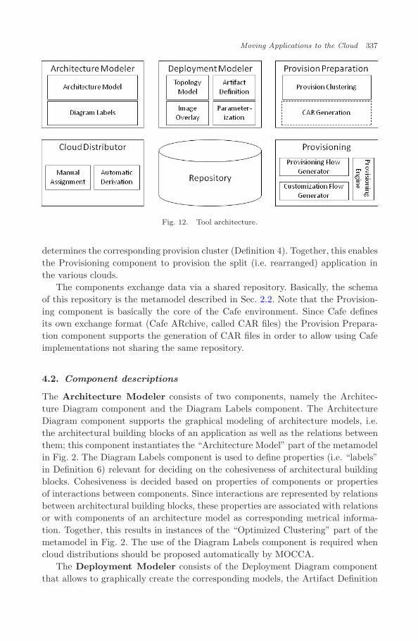
Figure 12 shows the overall architecture of the MOCCA tool. The tool consistsof several components supporting the various artifacts of the method proposed.Architecture models (Definition 5) are modeled using the Architecture Modeler.Deployment topologies and models, middleware deployments (Definition 2) as wellas deployment relevant parameters and installation relevant artifacts are specifiedby means to the Deployment Modeler. The cloud distribution (Definition 1), i.e.the split of the application is derived via the Cloud Distributor. Based on the clouddistribution and the middleware deployment the Provision Preparation component



Fig. 12. Tool architecture.

determines the corresponding provision cluster (Definition 4). Together, this enablesthe Provisioning component to provision the split (i.e. rearranged) application inthe various clouds.

The components exchange data via a shared repository. Basically, the schemaof this repository is the metamodel described in Sec. 2.2. Note that the Provision-ing component is basically the core of the Cafe environment. Since Cafe definesits own exchange format (Cafe ARchive, called CAR files) the Provision Prepara-tion component supports the generation of CAR files in order to allow using Cafeimplementations not sharing the same repository.

4.2. Component descriptions

The Architecture Modeler consists of two components, namely the Architec-ture Diagram component and the Diagram Labels component. The ArchitectureDiagram component supports the graphical modeling of architecture models, i.e.the architectural building blocks of an application as well as the relations betweenthem; this component instantiates the “Architecture Model” part of the metamodelin Fig. 2. The Diagram Labels component is used to define properties (i.e. “labels”in Definition 6) relevant for deciding on the cohesiveness of architectural buildingblocks. Cohesiveness is decided based on properties of components or propertiesof interactions between components. Since interactions are represented by relationsbetween architectural building blocks, these properties are associated with relationsor with components of an architecture model as corresponding metrical informa-tion. Together, this results in instances of the “Optimized Clustering” part of themetamodel in Fig. 2. The use of the Diagram Labels component is required whencloud distributions should be proposed automatically by MOCCA.

The Deployment Modeler consists of the Deployment Diagram componentthat allows to graphically create the corresponding models, the Artifact Definition



component, the Image Overlay component and the Parameterization component.The Deployment Diagram component supports the graphical modeling of thedeployment topology of an application, i.e. it instantiates the “Deployment Topol-ogy” part of the metamodel in Fig. 2; especially, the middleware deployment ofan application can be modeled. The Artifact Definition component allows specify-ing details about the implementation artifacts required to install a component inits runtime environment; this component instantiates the “Automatic Installation”part of the metamodel in Fig. 2. The artifacts needed are essentially the code filesor packages (such as WAR files, or OVF images) that implement the component.These can be reused across different applications, for example the implementationof a Web service can be used in several applications. Depending on its implemen-tation type, an artifact may be deployable on components of different types, i.e. aWAR file might be deployable on a component of type Apache Tomcat, or a com-ponent of type JBOSS. By defining artifacts representing virtual images (or partsthereof) as implementations of application components, the Image Overlay compo-nent supports overlaying the architecture of an application and virtual images. TheParameterization component allows defining both, deployment relevant propertiesand variability points of a component as well as the relations between them. Thus,this component is used to instantiate the “Deployment Parameterization” part ofthe metamodel in Fig. 2.

The Cloud Distributor is used to determine a cloud distribution for a givenapplication. A cloud distribution can be defined manually by using the ManualAssignment component. If the Diagram Labels component has been used to anno-tate the architecture model of an application with cohesion relevant properties, theAutomatic Derivation component can be used: it will automatically propose a clouddistribution based on the optimization algorithms described in Sec. 3.2.

The Provision Preparation component especially derives the provision clus-ter of an application based on the middleware deployment determined by using theDeployment Modeler and the cloud distribution determined by the Cloud Distrib-utor. The corresponding deep intersection is computed by the Provision Clusteringcomponent of the Provision Preparation. As a result, the application template ofthe rearranged application is build. Furthermore, the “CAR Generation” compo-nent could be used to generate the CAR file for the rearranged application, i.e. thefile format used by the Cafe tool and a proposed interchange format for compositecloud applications.

The Provisioning component is a subset of the Cafe environment as used inMOCCA; the corresponding functionality is described in Sec. 4.3 (see also Ref. 17).Basically, the Customization Flow Generator generates a customization workflowthat derives the properties required for provisioning and deployment of the rear-ranged application. This is an important step in the provisioning process as the cus-tomization flow gathers the required values to bind variability points either froma user or from the associated visible properties and overwrites the configurationsettings of the corresponding artifacts as indicated by the locators. For example,



EPR values or JNDI properties of components are overwritten with concrete val-ues obtained from the visible properties of other components. The customizationworkflow is used by the provisioning workflow generated by the Provisioning Flowcomponent. The provisioning flow is enacted by the Provisioning Engine to finallyinstall the rearranged application in the target cloud environments.

4.3. Usage of Cafe for performing actual deployment

Cafe maps OVF artifacts like virtual systems to separate components. Currently,Cafe assumes that a single OVF file represents a single component. Thus, in case aprovisioning cluster contains an OVF file that contains the virtual image of morethan one component (i.e. more than one virtual systems), this file must be splitinto separate OVF files manually. A straightforward extension of Cafe will eitherperform this split automatically (thus, using the existing Cafe unchanged) or willsupport OVF files with virtual images of multiple components.

From the deployment parameterization of an application (which is called “vari-ability model of an application template” in Cafe) the Cafe infrastructure generatesa so-called customization flow that deals with the binding of the variability pointscontained in the deployment parameterization. The provisioning flow is a workflowthat represents the variability points, their alternatives, their enabling conditionsand the dependencies between the variability points. The provisioning flow ensuresa complete and correct customization of the application during deployment. “Com-plete and correct” means that (i) each variability point is bound and (ii) the rulesimposed on the binding of variability points, i.e. which alternatives may be selectedand in which order the variability points are bound, are followed. The generationof customization flows from variability models is described in detail in Ref. 17.

The deployment topology and the automatic implementation artifacts of anapplication (called “application model” in Cafe) as well as the dependencies betweencomponents induced by the deployment parameterization are interpreted by theCafe provisioning environment in the following way: First a so-called “provisioningorder graph” is generated. The provisioning order graph specifies in which orderthe components of the application must be provisioned. Three rules apply here:(i) before a component can be provisioned all components that transitively containthis component must be provisioned; (ii) before a component can be provisioned, allits variability points that must be bound at pre-provisioning time must be bound.Thus, all components to which a given component is connected via a propertyalternative whose associated visible properties become only available at runtimemust be provisioned before the given component; (iii) components that do not haveany dependencies on each other can be provisioned in parallel.

A provisioning flow can be generated from the provisioning order graph thatperforms the provisioning in the right order as follows: For each node in the graphso-called “provisioning activities” are added to the workflow model, these are con-nected via control connectors that represent the dependencies. This way the three



rules above are ensured. The provisioning activities then contain activities to bindthe pre-provisioning variability points of a component by calling the provisioningflow who will then either prompt the user for inputs if the deployment parameteri-zation requires it or queries the already provisioned components for their respectivevisible properties. These are always already available as the ordering of the provi-sioning of the components follows rule (ii) above.

All already provisioned components in Cafe are represented by so-called “com-ponent flows” that provide a unified interface of components at different providersto the provisioning infrastructure. In order to deploy a component on an alreadydeployed component, the deploy operation of the component flow of this compo-nent is called with the location of the repository in which the component that mustbe deployed is located. In case the component to be deployed is a virtual image(for example an OVF image) the component flow that represents the hypervisor ofthe provider that will later run the OVF image is called along with the repositorylocation in which the customized OVF image is deployed. This operation is thenmapped by the component flow to a hypervisor-specific operation that starts a newvirtual image from a virtual image package such as OVF. When starting the newvirtual image the hypervisor also starts the activation engine which starts the corre-sponding scripts contained in the virtual image. In case other components must bedeployed on the infrastructure contained in the virtual machine, the component flowfor the hypervisor starts a component flow that can deploy other components onthe middleware component contained in the virtual machine. This component flowcan be developed specifically for the virtual image or can be a standard componentflow that makes use of the deployment interface of the component in the virtualmachine, for example, a standard component flow could copy a Web applicationarchive to a specific directory in the virtual machine or could deploy a processarchive via the deployment Web service of the BPEL18 engine contained in thevirtual machine. Thus a component flow that implements the deploy operation forcomponents that must be deployed on the middleware component in the virtualmachine must be deployed in the Cafe environment before the corresponding appli-cation can be provisioned.

5. Case Study

In this section, we report about the actual move of the sample application intro-duced in Sec. 2.3 into the cloud. First, the implementation of the architecturecomponents is described followed by their corresponding Deployment Parameteri-zation used by Cafe for the actual provisioning of the application. The associatedCafe artifacts and their relevance for the MOCCA method are described.

5.1. Application components

All components of the sample applications depicted in the architecture diagram(see Fig. 3) have been prototyped (with basic functionality only) by using open



source software. To facilitate their provisioning using Cafe a set of properties andVariability Points as well as their dependencies were identified. The Input Entrycomponent offers customer interaction through Java Server Pages. It also containsWeb service clients implemented in Java to interact with the Good Standing Ver-ifier and the Risk Assessor components. Those clients are initiated from the JavaServer Pages and their output is displayed to the customer. The Progress Monitorconstitutes another component used for customer interaction. It is also realized asa Java Server Page using a Web service client to obtain a list of all processed ordersfrom the Data Handler component. The good standing of a customer is evaluatedby the Good Standing Verifier component which is implemented as a Web ser-vice and is called by the Input Entry component. The Risk Assessor component isimplemented as a BPEL process, assessing the risk computed by the Good Stand-ing Verifier. If the risk is acceptable, the Risk Assessor initiates the processing ofthe order by the Order Processing component. The Order Processing component(another BPEL process) handles the actual ordering of an item. First, it verifiesthat the item is available by accessing the Stock Management component. If so, itremoves the item from the stock and stores the order information using the DataHandler component. The Stock Management component is realized as a Web ser-vice. It manages the items available to the ordering application. The Data Handlercomponent manages the persistent information about all orders processed. It is alsoimplemented as a Web service.

The general package format for all application components are WAR files withthe exception of the BPEL processes which are packaged as ZIP files. The InputEntry, Progress Monitor, and Good Standing Verifier are deployed on Apache Tom-cat, the Risk Assessor and Order Processing on Apache ODE, and the Stock Man-agement and Data Handler on JBoss which allows them to access a Hyper SQLDatabase (HSQLDB) through Hibernate. The required middleware is provided asthree virtual machine images. Corresponding to MOCCA’s deployment model, thefirst virtual image contains Apache Tomcat, the second contains Apache ODE, andthe third contains JBoss and HSQLDB.

5.2. Deployment parameterization used by Cafe

In order to be provisioned using the Cafe environment Variability Points of thecomponents have to be identified and made accessible to Cafe. Cafe may access andmanipulate any XML file within the component package during the provisioningprocess. The Cafe metamodel does currently not include Visible Properties butit treats them as Variability Points that are filled by the provisioning infras-tructure. All properties (i.e. instances of Property) of the application componentsare thus transformed into Variability Points for the usage in Cafe. Instead ofallowing to import Visible Properties for a component of a specific type, Cafeallows the import of the Variability Points for a component type, i.e. a con-crete application server. For the sample application these Variability Points are



the addresses (e.g. URLs) of the components themselves as well as the addressesof accessed components since they are unknown until after provisioning. For theItem Manager and Data Handler components an additional property is the addressof a Hyper SQL Database. To ensure that Cafe can process Variability Points

they have to be accessible, i.e. may not reside in compiled source files. Web servicesoffered and accessed by the components are therefore configured through WSDLfiles. During the provisioning process Cafe may adjust the SOAP addresses of theWSDL ports in those files. To configure the database access Hibernate also offersconfiguration through an XML file that can be set automatically by the Cafe pro-visioning infrastructure.

5.3. Provisioning the application using Cafe

Utilizing MOCCA tools, the application architecture model is modeled and thecloud distribution is computed as described in Sec. 3.3 and based on the labelsdiscussed there. This information is then used to create the Cafe artifacts necessaryfor provisioning. Semantics and usage of these artifacts have been discussed inSec. 4.3. Please consider that in practical settings these tools will import existingmodels.

Since MOCCA and Cafe use the same metamodel regarding the models fordeployment topology, automatic installation, and deployment parameterizationdepicted in Fig. 2, Cafe tools integrate with those of the MOCCA architecturealmost seamlessly. Its application model can be obtained from the MOCCA deploy-ment model. However, to provision the sample application this model needs toconform to the provision cluster. Currently, Cafe does not support to overlay anapplication model with the hyper edges of a cloud distribution to obtain provisionclusters. This is due to the fact that Cafe originally does not support the notionof multiple clouds and considers every modeled component to be instantiated onlyonce. Therefore the splitting of middleware components across different clouds, asdescribed by Definitions 3 and 4, has to be made explicit in Cafe’s application model.Respective to the provision cluster of the sample application shown in Fig. 13 theApache Tomcat component is split into two components. One contains the InputEntry component and is hosted in Cloud 1. The other contains the Good StandingVerifier and Progress Monitor components and is hosted in Cloud 2. Other middle-ware components do not have to be split up since only one single instance is requiredof those. Note, that a Cafe application model can be derived from a MOCCA deploy-ment model by making the distribution explicit. However, the round-trip back isnot possible. Thus the Cafe application model must be extended with informationthat allows split components to be reassembled again as required by the MOCCAdeployment model.

The application model is further used to map components to their implemen-tation by referencing deployment packages such as WAR and ZIP files or OVFImages. Access to Variability Points is possible through the definition of XPath



GoodStandingVerifier

ProgressMonitor

InputEntry

RiskAssessor

OrderProcessor

DataHandler

StockManagement

Cloud 2

Cloud 1

ApacheODE

ApacheTomcat

JBOSS+HSQLDB

Fig. 13. Provision cluster of the sample application.

expressions altering the XML files inside those packages. A screenshot of theapplication diagram modeler is shown in the appendix.

In addition to the application model, a so-called component binding is needed.The component binding is used to associate component flows with the components.These are needed to perform the actual provisioning of components as describedin Sec. 4.3. They are specified by End Point References through which the flowmay be accessed. Since the application model represents the provision cluster, eachcomponent may have an individual component flow depending on the cloud to whichis it provisioned. A screenshot of the component binding modeler is shown in theappendix.

The final task before provisioning the application is providing the neces-sary deployment parameterization by specifying the Variability Points andtheir dependencies. The Variability Points of the sample application consistof addresses of the Web services offered and accessed by the components. Respect-ing the dependencies of these Variability Points, the provisioning flow for theapplication is computed automatically. The provisioning flow then performs theprovisioning by executing the component flows of the individual components inthe right order, respecting the dependencies of components’ Variability Points.Regarding the variability model created using the variability modeler tool, depictedin appendix the following flow is generated (sketched only in what follows). Firstmiddleware components are provisioned which allow the computation of applicationcomponents’ addresses. Circular dependencies are supported by the configurationof components during runtime. Second, the Stock Management, Data Handler, andGood Standing Verifier are provisioned in parallel since they do not depend on



any other component. Then the Variability Points of the Progress Monitor andOrder Processor are known and they can be deployed subsequently. Afterwards, theRisk Assessor and last the Input Entry component are provisioned.

5.4. Application management in Cafe

Cafe allows provisioning instances of different applications. To make an applica-tion (called application template in Cafe) known to the Cafe system, it must beuploaded to the Cafe system via the Cafe portal. Before uploading, all generatedartifacts (code, application model, variability model and component bindings) mustbe packaged into a Cafe Application Archive (CAR) file. This file can then beuploaded to a Cafe environment. To provision a new instance of an application, acustomer selects one of the available templates in the Cafe portal. Then the cus-tomer must bind all Variability Points that require decisions by the customer.During the binding of the Variability Points the customer is guided by thecustomization flows generated from the Variability Point. Once all customer-related Variability Points have been bound, the corresponding provisioning flowis executed that makes use of the component flows and the customization flows thatbind provisioning-related Variability Points, to setup the whole application.

6. Related Work

Given the focus of this paper, related work can be clustered into two main categories:infrastructure topologies and composite application approaches as well as resourceoptimization approaches in Grids and Clouds.

6.1. Infrastructure topologies and composite applications

Several approaches that aim at describing and provisioning complex infrastructuretopologies exist. Virtual images as basic building blocks for deploying complexmiddleware topologies on top of IaaS clouds (Infrastructure as a Service) are inves-tigated in Ref. 19: the conclusion is that individual virtual images are not powerfulenough to capture complex infrastructure requirements such as multiple applicationservers that communicate with authentication servers and databases, for example.Thus, Ref. 19 introduces a so-called “virtual appliance model” that allows definingsolutions that are composed of multiple configurable virtual images that can beautomatically deployed and run in separate IaaS clouds such as Amazon EC2.20

The approach presented in Ref. 19 differs from our approach presented in this paper:while Ref. 19 focuses solely on reusable virtual images and their composition, ourapproach focuses on existing applications and shows how they can be split (in anoptimal manner) and moved to (multiple) clouds. Furthermore, virtual images inour approach are optional, i.e. we can also move applications to the cloud with-out assuming virtual images but deploy applications on top of middleware alreadyavailable in the cloud. The approach presented in Ref. 19 is based on the approach



presented in Ref. 21 which offers a semantically rich metamodel to model complexdeployment models similar to those, that we allow to model in MOCCA. How-ever, the difference is, that their approach employs a very rich metamodel while weemploy a simple, generic metamodel. While their focus is to capture existing mid-dleware in templates, which requires the complex definition of the template beforeapplications can be modeled. Our model allows to only define those variabilitiesthat are absolutely needed to configure and deploy an application. However, in casecomplex component types are needed and offered by providers, application mod-elers can import the variability models of the component types and can integratethem in the application variability model, thus reusing the work of the providerand having the same effect as the approach in Ref. 21.

Elastra22 and Rightscale23 offer cloud management services on top of IaaSclouds. Elastra for example provides special languages (ECML, EDML) to describethe infrastructure components of an application such as application servers,databases and their connections. However, concrete resources must be manuallyassigned to these components, and application modules must be manually installedon top of the components. 3tera30 offers modeling and deployment of applicationsbased on pre-defined virtual images that can then be deployed in a data center. Allof these approaches focus on the management of resources and applications assum-ing that both are modeled for and managed within a particular target environment.In contrast, our approach is focused on rearranging existing composite applicationssuch that they can be moved to the cloud and can be automatically provisionedacross different providers; especially, our approach is independent from particulartarget environments.

The application packaging standard (APS)24 focuses on the description of Webapplications including, for example, UI components, databases and configuration ofWeb servers. APS is limited to Web applications and does not allow the annotationof parameters to individual components that would allow the partitioning of theapplication across multiple Web servers and thus is unsuitable for the purpose ofMOCCA. Several approaches exist such as those described in Refs. 25–27 that dealwith the description of composite service-oriented applications in terms of compositeservices that consist of a set of other services. However, all these approaches donot allow the modeling of infrastructure components and thus are unsuitable todescribe the infrastructure components of different clouds on which different partsof an application must be deployed.

6.2. Resource optimization approaches in grids and clouds

In MOCCA we treat the distribution of application and infrastructure componentsacross different clouds as an optimization problem that solves the task of findingan optimal distribution of components given a set of parameters.

In the Grid28 the optimization of the distribution and scheduling of jobs acrossthe available resources is an important problem. The component to deal with this



optimization is the resource broker or resource scheduler.28–30 Grid users can send,for instance, job submissions to the broker. The broker then decides which resourceswill perform the job based on various criteria such as resource utilization, cost ofnon-functional properties of different resources. Different algorithms exist that opti-mize the scheduling of the required resources. In Ref. 31, an overview and compar-ison of these optimization algorithms is given. The problem of job scheduling in aGrid is different from the MOCCA approach, as in MOCCA the distribution acrossdifferent infrastructure resources is done pre-deployment and not when a request forcomputation is submitted to an application. Thus the algorithms commonly used inresource brokers focus on the optimization of the distribution of all jobs submittedto a Grid over the available infrastructure. The framework presented in Ref. 32 canact as such a resource broker for application resources in a cloud as it allows to plug-in several algorithms to optimize the distribution of tenants in a cloud application.An approach based on game theory is taken by Lee et al.34 to optimize the allocationof resources for distributed applications in a single cloud given a constrained set ofavailable resources. In Ref. 35, the OpenNebula virtual infrastructure managementframework is introduced that includes the Haizea resource scheduling manager toschedule workload across different virtual machines. The Eucalyptus cloud manage-ment framework36 contains similar resource allocation algorithms that allow usersof the framework to start and stop virtual machines without having to deal withthe concrete resource allocation and scheduling. All these approaches operate at alower level than the MOCCA approach as they focus on single clouds and Grids andhow to optimize the resource allocation in a single cloud or Grid, whereas MOCCAhelps architects with the decision how to split applications across different cloudsand thus has a different focus. The resource allocation algorithms researched forGrids and clouds can then be used by the individual cloud providers to optimizethe resource allocation for the components they have been given to host by theapplication architects as a result of applying the MOCCA method.

7. Conclusion

In this paper, we proposed a method (the MOCCA method) for solving the move-to-cloud problem. This method has been described in terms of the various stepsto be performed and artifacts to be created in order to move an application tothe cloud. A metamodel has been presented that formally describes these artifactsand their relations. The artifacts are mainly application models that are enrichedby deployment information and labels. The move-to-cloud problem especially sub-sumes the problem of rearranging the components of an application into groupsthat might be provisioned into different clouds: this problem has been formalizedas an optimization problem (cloud distribution problem) and a solution for solvingthis problem has been worked out.

We presented the architecture of a tool suite that supports the modeling of theartifacts of the MOCCA method. Also, it supports the automatic derivation of cloud



distributions and provision clusters, i.e. it solves the cloud distribution problem.Finally, the provision clusters are automatically provisioned into their target clouds.Thus, the MOCCA method and accompanying tool suite solves the move-to-cloudproblem in practical situations. A sample application has been implemented andmoved to the cloud to verify the viability of the MOCCA method and tools.

Appendix A. Screenshots

The tool architecture shown in Fig. 12 has been realized based on both, graphicaltools as well as tree-based tools (or tree-based tools, respectively). The graphicaltools lean more towards domain experts while the tree-based tools are more gearedtowards supporting expert development personnel. The following subsections showsome screenshots of both kinds of tools.

A.1. Graphical tools

The graphical tools have been realized based on the Cafe framework,7 which inturn is based on EMF and GMF. These Eclipse-based technologies support thedevelopment of editors for arbitrary metamodels and graphical representations ofthese. The Cafe metamodel is defined in EMF while GMF is used to specify thegraphical representation of metamodel elements.

Figure 14 shows the implemented editor for specifying application models. Onthe upper left an Eclipse project containing the models and other artifacts, such

Fig. 14. Modeling the Cafe application diagram.



as code, of the sample application is shown. The representation of the applica-tion model is opened in the main view. On the top the JBoss middleware compo-nent is modeled. It contains the Stock Manager and Order Manager components.The implementation of the JBoss component is specified as ProviderSupplied. Thecontained components reference the WAR files which hold their implementationartifacts. These files are also visible in the project explorer on the left side.

Variability Points of the components and their dependencies are modeled inthe variability diagram shown in Fig. 15. The Variability Point of the ApacheTomcat component (TomcatEPR) representing the end point reference of theApache Tomcat servlet container is visible on the top left in the main view. Ithas one free Alternative as described in Sec. 2.2 which is the hostname of theApache Tomcat instance. It is filled during the provisioning process. Since theGood Standing Verifier is hosted on the Apache Tomcat component as seen inFig. 14 the URL of the offered service (represented by the Variability Point

GSERP) depends on the TomcatEPR Variability Point. It is filled once theTomcatEPR Variability Point is known. The Variability Point of the InputEntry (InputEntryGSEPR) depends on the URL of the Good Standing Verifier

Fig. 15. Modeling the variability diagram of the sample application.



Fig. 16. Specifying component bindings.

since it uses this component. From the variability points depicted in this diagramthe customization flows can be generated as described in Sec. 4.3. Additionallythese dependencies serve as input to the provisioning flow’s decision in which orderto provision the individual components.

The provisioning flow initiates the component flows of application componentsto provision an application instance. These component flows are associated withan application component through component bindings. In Fig. 16, the componentbinding for the JBoss component is selected in the main view of Eclipse. In theproperties view on the lower side the properties of this component are displayed.This is where the component JBoss modeled in the application diagram is refer-enced. The element currently selected in the properties view shows the End PointReference of the component flow for that referenced component. The action ele-ment specifies the purpose for which the component flow is used. In this case itis for provisioning. Additional component bindings may also be specified to ref-erence component flows implementing other actions. Those include adding othercomponents after provisioning the referenced component or deprovisioning it.

Having packaged the sample application using the CAR export file wizard of theapplication modeler, the application can be uploaded to the Cafe Portal. Havinguploaded the application it becomes available under the templates tab (as shownin Fig. 17) and customers can subscribe to that application.



Fig. 17. The sample application in the Cafe portal.

A.2. Tree-based tools

The tree-based tools have been realized by using VBMF,11 which is an Eclipse-basedtool supporting model driven development of applications. Especially, it supports aneasy way to specify metamodels and generates corresponding tree-based modelingtools. Based on Fig. 2, the metamodels denoted as “model types” in that figurehave been specified in VBMF and the corresponding modeling tools for tree-basedspecification of architecture models, deployment topology etc. result.

Figure 18 shows the tool allowing to model components of an architecturemodel (the “boxes”) and also of deployment models. The WebSphere component is

Fig. 18. Modeling components.



high-lighted in the left part of the screen and the right part shows the propertiesof that component, e.g. its name and its type (in this case “AppServer”). The sub-components of WebSphere application server are the Risk Assessor as well as theOrder Processor components (see Fig. 4).

The “arrows” of an architecture model are specified as component relations asshown in Fig. 19. The left side of the screenshot high-lights the component relationInputEntry GoodStandingVerifier and the right side show its properties especiallythat it begins at the Input Entry component and ends at the Good Standing Verifiercomponent (as shown in Fig. 3).

The fact, that the MWStack component encompasses (amongst others) theWebSphere component and the DB2 component (see Fig. 5) has been specifiedin Fig. 20.

Fig. 19. Modeling relations.

Fig. 20. Modeling composite components.



Fig. 21. Specifying implementations.

Fig. 22. Specifying artifacts.

Fig. 23. Modeling labels.



Fig. 24. Labeling relations.

Fig. 25. Labeling components.

Fig. 26. Modeling properties.



Fig. 27. Modeling visible properties.

The information from Fig. 5 that WebSphere is realized by an implementationof type OVF and that this OVF file is a BLOB Artifact having a certain FileRef

attribute is given in Figs. 21 and 22, respectively.Figure 23 gives an example of modeling labels. The label AMOUNT OF DATA

high-lighted and got the value 200 assigned. This label has been associated to thecomponent relation InputEntry GoodStandingVerifier in Fig. 24. The other labelcalled TRUST has been associated with the DB2 component in Fig. 25.

The specification of properties is depicted in Fig. 26: the property hostnamehas been shown that has no value assigned (according to the situation modeled inFig. 5). Figure 27 also specifies hostname as a visible property now having the valuefranksDB2 (see Fig. 5).

References

1. M. Armbrust, A. Fox, R. Griffith, A. D. Joseph, R. Katz, A. Konwinski, G. Lee,D. Patterson, A. Rabkin, I. Stoica and M. Zaharia, Above the Clouds: A BerkeleyView of Cloud Computing, Technical Report (2009).

2. R. Buyya, C. S. Yeo, S. Venugopal, J. Broberg and I. Brandic, Cloud computing andemerging IT platforms: Vision, hype, and reality for delivering computing as the 5thutility, Future Generation Computer Systems 25 (2009) 599–616.

3. S. Jha, A. Merzky and G. Fox, Using clouds to provide grids higher-levels of abstrac-tion and explicit support for usage modes, Concurrency and computation: Practiceand experience, Special Issue of the OGF (2009).

4. National Institute of Standards and Technology, Draft NIST Working Definition ofCloud Computing (2009), http://csrc.nist.gov/groups/SNS/cloud-computing/cloud-def-v12.doc.

5. Open Cloud Manifesto (2009), http://www.opencloudmanifesto.org/Open%20Cloud%20Manifesto.pdf.

6. F. Leymann, Cloud computing: The next revolution in IT, in Proc. of the 52th Pho-togrammetric Week (Stuttgart, Germany, 2009).



7. R. Mietzner, T. Unger and F. Leymann, Cafe: A generic configurable customizablecomposite cloud application framework, in Proc. of the 17th Intl. Conf. on CooperativeInformation Systems, CoopIS (Springer-Verlag, Berlin, Heidelberg, 2009).

8. S. Weerawarana, F. Curbera, F. Leymann, T. Storey and D. F. Ferguson, Web ServicesPlatform Architecture (Prentice Hall, 2005).

9. DMFT Standard: Open Virtualization Format Specification, Document Number:DSP0243 (2009), http://www.dmtf.org/standards/published documents/DSP02431.0.0.pdf.

10. The ACME Project, http://www.cs.cmu.edu/∼acme/.11. H. Tran, U. Zdun and S. Dustdar, View-based and model-driven approach for reducing

the development complexity in process-driven SOA, in Proc. of the Intl. Conf. onBusiness Processes and Services Computing (Leipzig, Germany, 2007).

12. BPMN 1.1, http://www.bpmn.org/Documents/BPMN 1-1 Specification.pdf.13. L. Hohmann, Beyond Software Architecture (Addison-Wesley, 2003).14. M. R. Garey and D. S. Johnson, Computers and Intractability — A Guide to the

Theory of NP-Completeness (W.H. Freeman & Co., 1990).15. S. Kirkpatrick, C. Gelatt and M. Vecchi, Optimization by simlated annealing, Science

220 (1983).16. O. Danylevych, D. Karastoyanova and F. Leymann, Optimal stratification of trans-

actions, in Proc. of the 4th Intl. Conf. on Internet and Web Applications and Services(2009), pp. 493–498.

17. R. Mietzner and F. Leymann, Generation of BPEL customization processes for SaaSapplications from variability descriptors, in Proc. of the Intl. Conf. on Services Com-puting (Washington, DC, USA, 2008).

18. BPEL, www.oasis-open.org/committees/wsbpel/.19. A. Konstantinou, T. Eilam, M. Kalantar, A. Totok, W. Arnold and E. Snible, An

architecture for virtual solution composition and deployment in infrastructure clouds,in Proc. of the 3rd Intl. Workshop on Virtualization Technologies in Distributed Com-puting (VTDC, 2009).

20. Amazon EC2, http://aws.amazon.com/ec2/.21. K. El Maghraoui, A. Meghranjani, T. Eilam, M. H. Kalantar and A. V. Konstantinou,

Model driven provisioning, bridging the gap between declarative object models andprocedural provisioning tools, in Proc. of the 7th Intl. Middleware Conference (2006),pp. 404–423.

22. ELASTRA, http://www.elastra.com/.23. RightScale, http://www.rightscale.com/.24. SWSoft Inc. Application Packaging Standard (APS) (2007), http://apsstandard.com/

r/doc/package-format-specification-1.0.pdf.25. B. Benatallah, M. Dumas and Q. Z. Sheng, Facilitating the rapid development and

scalable orchestration of composite web services, Distributed and Parallel Databases17(1) (2005) 5–37.

26. Open SOA Collaboration (OSOA), SCA Service Component Architecture,Assembly Model Specification Version 1.00 (2007), http://www.osoa.org/download/attachments/35/SCA AssemblyModel V100.pdf.

27. F. Rosenberg, P. Leitner, A. Michlmayr, P. Celikovic and S. Dustdar, Towards com-position as a service — a quality of service driven approach, in Proc. of the Intl. Conf.on Data Engineering (Shanghai, China, 2009), pp. 1733–1740.

28. I. Foster and C. Kesselman, The Grid: Blueprint for a New Computing Infrastructure(Morgan Kaufmann, 2004).

29. R. Buyya, D. Abramson and J. Giddy, Nimrod-G resource broker for service-orientedgrid computing, IEEE Distributed Systems Online 2(7) (2001).



30. 3tera, http://www.3tera.com/.31. C. Yang, P. Shih and K. Li, A high-performance computational resource broker for

grid computing environments, in Proc. of the 19th Intl. Conf. on Advanced Informa-tion Networking and Applications, Vol. 2, IEEE Computer Society (Washington, DC,USA), pp. 333–336.

32. K. Li, Job scheduling and processor allocation for grid computing on metacomputers,Journal of Parallel and Distributed Computing 65(11) (2005) 1406–1418.

33. C. Fehling, F. Leymann and R. Mietzner, A framework for optimized distribution oftenants in cloud applications, in Proc. of the 3rd International Conference on CloudComputing (Miami, USA, 2010), pp. 252–259.

34. C. Lee, J. Suzuki, A. Vasilakos, Y. Yamamoto and K. Oba, An evolutionary game theo-retic approach to adaptive and stable application deployment in clouds, in Proc. of the2nd Workshop on Bio-Inspired Algorithms for Distributed Systems (ACM, New York,NY, 2010), pp. 29–38.

35. B. Sotomayor, R. S. Montero, I. M. Llorente and I. Foster, Virtual infrastructuremanagement in private and hybrid clouds, IEEE Internet Computing 13(5) (2009)14–22.

36. D. Nurmi, R. Wolski, C. Grzegorczyk, G. Obertelli, S. Soman, L. Youseff andD. Zagorodnov, The eucalyptus opensource cloud-computing system, in Proc. of the9th IEEE/ACM Intl. Symposium on Cluster Computing and the Grid-Volume (IEEEComputer Society, 2009), pp. 124–131.