MSc. Thesis

A novel method to measure parameters of amicrowave cavity

Balazs Gyure

Thesis advisor: Ferenc SimonProfessorDepartment of PhysicsInstitute of PhysicsBME

Budapest University of Technology and Economics

BME2014.

1

ContentsA szakdolgozat kiırasa 4

Onallosagi nyilatkozat 5

Koszonetnyilvanıtas 6

1 Motivation for the work 7

2 Theoretical basics 92.1 Microwave cavity . . . . . . . . . . . . . . . . . . . . . . . . . . . . . . . . 9

2.1.1 Basics of the microwave cavity . . . . . . . . . . . . . . . . . . . . . 92.1.2 Cavity transient . . . . . . . . . . . . . . . . . . . . . . . . . . . . . 10

2.2 Traditional methods of measuring the quality factor of cavities . . . . . . . 102.2.1 Frequency sweep . . . . . . . . . . . . . . . . . . . . . . . . . . . . 102.2.2 AFC based method . . . . . . . . . . . . . . . . . . . . . . . . . . . 122.2.3 Performance benchmarks of Q measurement methods . . . . . . . . 13

2.3 The microwave components . . . . . . . . . . . . . . . . . . . . . . . . . . 142.3.1 Microwave mixer . . . . . . . . . . . . . . . . . . . . . . . . . . . . 142.3.2 PIN diode . . . . . . . . . . . . . . . . . . . . . . . . . . . . . . . . 16

2.4 Time and frequency-domain microwave measurements . . . . . . . . . . . . 17

3 Results and discussion 193.1 Transient of an RF circuit . . . . . . . . . . . . . . . . . . . . . . . . . . . 193.2 Experimental setup to detect cavity transients . . . . . . . . . . . . . . . . 223.3 Theoretical description of the measurement . . . . . . . . . . . . . . . . . . 24

3.3.1 The cavity parameters . . . . . . . . . . . . . . . . . . . . . . . . . 243.3.2 The switch off transient . . . . . . . . . . . . . . . . . . . . . . . . 263.3.3 The switch on transient . . . . . . . . . . . . . . . . . . . . . . . . 263.3.4 Transients for arbitrary coupling . . . . . . . . . . . . . . . . . . . 27

3.4 Time-domain cavity transients . . . . . . . . . . . . . . . . . . . . . . . . . 283.4.1 Analysis in the time-domain . . . . . . . . . . . . . . . . . . . . . . 303.4.2 Analysis in the frequency-domain . . . . . . . . . . . . . . . . . . . 313.4.3 Effect of significant detuning . . . . . . . . . . . . . . . . . . . . . . 31

3.5 Performance of the novel method . . . . . . . . . . . . . . . . . . . . . . . 34

4 Summary 35

A The transients in an equivalent circuit model 37

B Additional methods considered 39B.1 High frequency sweep . . . . . . . . . . . . . . . . . . . . . . . . . . . . . . 39B.2 Lock-in quadrature detection . . . . . . . . . . . . . . . . . . . . . . . . . . 40B.3 Lock-in higher harmonics . . . . . . . . . . . . . . . . . . . . . . . . . . . . 41

2

C Measurements on a superconducting microwave cavity 42C.1 Construction of the superconducting cavity . . . . . . . . . . . . . . . . . . 42C.2 Measurements on the superconducting cavity . . . . . . . . . . . . . . . . . 43

3

A szakdolgozat kiırasaA radiofrekvencias impedancia meres a roncsolasmentes anyagvizsgalati modszerek

egyik legelterjedtebb aga, mely soran az anyag es radiofrekvencias sugarzas koztikolcsonhatast vizsgaljuk. Ezek kozott egy fontos alteruletet kepez az anyagok mikro-hullamokkal valo vizsgalata. Ennek egyik oka, hogy a mikrohullamok hullamhosszakicsi, eloallıtasuk aranylag konnyu, es rendelkezesre allnak fejlett laboratoriumi beren-dezesek. Laboratoriumban a mikrohullamu impedancia meres egyik leggyakrabbanhasznalt fajtaja az un. ureg-perturbacios technika. Ennel a merestechnikanal egy mikro-hullamu uregbe helyezett minta valtoztatja meg az ureg parametereit, elsosorban a Q,un. josagi tenyezojet. A Q meresere a legelterjedtebb modszer az uregre erkezo mikro-hullamu sugarzas frekvenciajanak folyamatos megvaltoztatasa (’sweep’-elese). E modszerhatranya, hogy a sweepeles soran nem kielegıto a frekvencia pontos valtozasanak idobeniegyenletessege. Az MSc diplomamunka soran egy teljesen uj, idodomenbeli Q mereslehetosegeit kellene elmeleti es kıserleti uton megvizsgalni. A javaslat lenyege, hogy azuregre impulzusszeruen adjuk ra a mikrohullamot, majd az ureg tranziens valaszabolhatarozzuk meg a josagi tenyezojet es sajat-frekvenciajat. Amennyiben a felvetes sikeres,ki kell dolgozni a merestechnikat a gyakorlatban, a meres hibajat, stabilitasat ellenoriznies a hagyomanyos merestechnikaval osszehasonlıtani.

Onallosagi nyilatkozatAlulırott Gyure Balazs, a Budapesti Muszaki es Gazdasagtudomanyi Egyetem

hallgatoja kijelentem, hogy ezt a szakdolgozatot meg nem engedett segedeszkozok nelkul,sajat magam keszıtettem, es csak a megadott forrasokat hasznaltam fel. Minden olyanszovegreszt, adatot, diagramot, abrat, amelyet azonos ertelemben mas forrasbol atvettem,egyertelmuen, a forras megadasaval megjeloltem.

Budapest, 2014. majus 3.

Gyure Balazs

KoszonetnyilvanıtasSzeretnem megkoszonni temavetomnek, Simon Ferencnek a sok evi kitarto tanıtasat

es tamogatasat. Emelett koszonom a Fizika tanszek munkatarsainak, Horvath Belanakes Bacsa Sandornak a felhasznalt kulonleges eszkozok elkeszıteset.

Koszonom Markus Bencenek az elmeleti szamolasokban nyujtott segıtseget. Koszonoma tanacsokat Holczer Karolynak es Janossy Andrasnak, nelkuluk az elert eredmenyek nemjottek volna letre.

Support by the European Research Council Grant Nr. ERC-259374-Sylo is acknowl-edged.

1 Motivation for the workThe RF impedance measurement is one of the most common methods of non-

destructive tests, which measures the interactions of matter and radio frequency radiation.An important subcategory is the measurement using microwaves. Some reasons for thisare that the wavelength of microwaves is smaller, their generation is relatively cheap, andthere is advanced laboratory equipment available.

Their place in communication (mobile phones, GPS satellites) is a further motivationfor the use of microwaves. MRI devices used in modern medicine also work within themicrowave frequency-domain, as do commercial and military radars. For all these reasonsmicrowave techniques for the tests of new materials have become very important andwidespread.

One of the most commonly used techniques for microwave impedance measurementsis the so-called cavity perturbation technique. We place the sample in a microwave cavityand monitor the changes in the cavity’s properties, namely the resonance frequency, f0,and the quality factor, Q. The conductivity of the sample can be calculated from theseparameters ([1]).

The aim is to improve the traditional techniques which measure the resonance fre-quency and quality factor of microwave cavities. The traditional methods have severaldrawbacks. These techniques all work based on measuring the shape of the resonancecurve while sweeping the irradiation frequency. For this reason, they suffer from thefrequency instability of the microwave source. Measurements made this way do not com-pletely reproduce their results due the fact that the size of the frequency steps may differbetween measurements. Additionally, when we measure the shape of a resonance curve,most of the time is spent measuring less relevant data outside the cavity resonance curve;this greatly increases the final noise of the measurement. One additional problem is thatgreat power differences are measured during a frequency sweep, which may be a limitingfactor due to the finite dynamic range of detectors.

Historically, the issues faced in NMR (nuclear magnetic resonance) technique showeda similarity with ones presented herein. The width of an NMR resonance is often just 1Hz, while its base (or Larmor) frequency is in the few 100 MHz range. The previouslyused continuous wave (CW) NMRs had great difficulty finding and exciting thin resonancepeaks. The main reason for this was the low frequency stability of the generators, whichhas to be frequency swept in such studies. The aforementioned problem of measuring off-resonance data for most of the time also limits the measurements. We have a similar issuein the study of microwave cavities. Typically as a rule of thumb, a cavity resonance curveis measured for a frequency sweep of 10-30 times broader than the resonance linewidthitself, i.e. the measurement time is not used effectively. The solution for NMR was to usepulse operation. For this improvement, the development of the so-called Fourier transformNMR, Richard R. Ernst received the Nobel Prize in Chemistry in 1991.

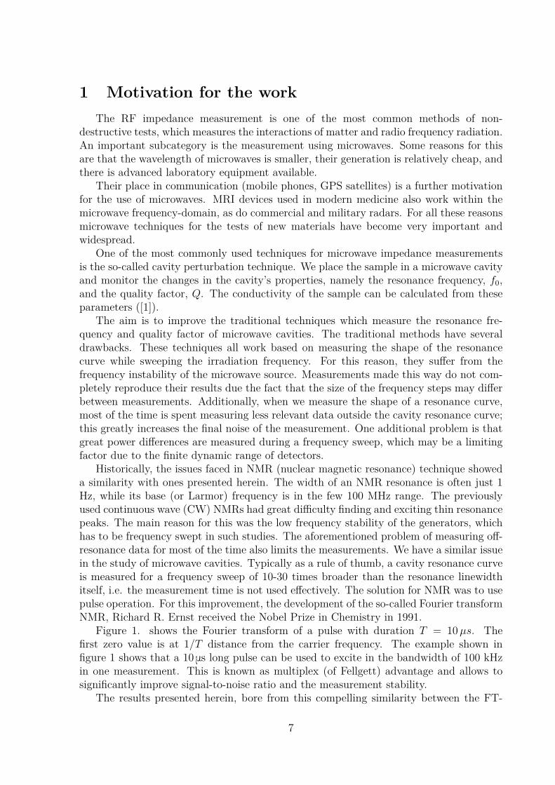
Figure 1. shows the Fourier transform of a pulse with duration T = 10µs. Thefirst zero value is at 1/T distance from the carrier frequency. The example shown infigure 1 shows that a 10 μs long pulse can be used to excite in the bandwidth of 100 kHzin one measurement. This is known as multiplex (of Fellgett) advantage and allows tosignificantly improve signal-to-noise ratio and the measurement stability.

The results presented herein, bore from this compelling similarity between the FT-

7

Figure 1: Fourier transform of a 10 μs long 1 MHz pulse and schematics of a typicalexcitation peak. The figure demonstrates that in NMR a broad frequency range is excitedsimultaneously.

NMR and the challenges we faced in the measurement of the cavity parameters.The primary motivation for this work was to develop a novel, yet unknown method for

these measurements with the hope of having a similar or superior performance. Duringthis work we found that the measurements of the cavity transient (the cavity’s response topulse signals) cannot be described by the theory found in the literature. The understand-ing of the cavity transient offers an opportunity for the development of novel measurementtechniques.

8

2 Theoretical basics

2.1 Microwave cavity2.1.1 Basics of the microwave cavity

An RLC circuit made of lumped elements cannot be used in the microwave frequency-domain, so instead, a cavity may be used as a resonator, whose walls are made of a highlyconductive material, usually copper. The dimensions of the cavity are comparable to thewavelength of the microwave radiation. Excited on its resonance frequency, a cavity canmaintain a standing wave mode, which is the superposition of the waves reflected fromthe cavity walls. A cavity is capable of maintaining several modes, whose properties arebased on the shape and size of the cavity. A large microwave field builds up when it iscoupled to a waveguide. When coupling to the cavity, care must be taken to match thedesired mode in the cavity to the mode in the waveguide.

Figure 2: Electromagnetic field in the cavity and the waveguide (dashed line: magneticfield, continuous line: electric field) [2].

It is generally known that the quality factor (Q) sets the magnitude of the electro-magnetic field in the cavity in the stationary state.

Q = 2π stored energy in the systemdissipated energy per period = f0

∆f (1)

f0 is the resonance frequency, ∆f is the full width at half maximum (FWHM) of theresonance curve. Using this relation between the Q factor and the FWHM is the mostwidely used method of measuring the Q factor.The Q factor of a cavity depends on the physical properties of the cavity, any sampleplaced in it and the coupling [2].

9

1Q

= 1Qempty cavity

+ 1Qsample

+ 1Qcoupling

(2)

1Q

= 1Q0

+ 1Qcoupling

(3)

Q is the quality factor for the whole system and Q0 for the cavity without the couplingtaken into account (uncoupled cavity). Qempty cavity is also called unloaded cavity. Criticalcoupling is achieved when there is no reflection from the cavity in the stationary state. Itcan be shown that in this case Qcoupling = Q0.

2.1.2 Cavity transient

A cavity cannot respond to arbitrarily rapid changes to the exciting microwave fre-quency or power. It is understood, as the large microwave field in the cavity cannot beinstantaneously built up. According to Ref. [2], the microwave voltage during the cavitytransient reads:

V = V0 · exp(−ω0t

Q

). (4)

Measurements were made of the cavity transient, as shown later, that found thatthe measured characteristic time differs from the one found in Ref. [2]. The measuredtransients for the cavity transient’s power and voltage are:

p(t) = p0 · exp(−tω0

Q

), (5)

V (t) =√p0Z0 · exp

(−tω0

2Q

)· exp (iω0t) . (6)

where p0 is the power of the source, ω0 = 2πf0, Z0 is the wave impedance of the microwavewaveguide and The phase was omitted in the expression of the reflected microwave voltage.

2.2 Traditional methods of measuring the quality factor of cav-ities

2.2.1 Frequency sweep

This is the most conventional and straightforward method to measure f0 and Q ofcavities. A microwave radiation is applied to the cavity to measure the reflection onthe cavity or transmission through the cavity. By continuously changing the microwavefrequency, we measure the frequency dependence of the cavity, namely the frequency-dependent reflection or transmission through the cavity. For both the reflection andtransmission measurements, we obtain a Lorentzian lineshape for the incident power onthe detector. Generally, the reflected or transmitted microwave power is measured using apower detector. To measure the signal, a Lock-in amplifier is used: the power of the sourceis chopped (or amplitude modulated). It is also possible to use an oscilloscope to measurethe signal, in this case there is no need for chopping and the resonance curve is monitored

10

Figure 3: Basic frequency sweeping methods using a lock-in amplifier and an oscilloscope.

real-time. For the latter measurement, a larger bandwidth is used, which increases themeasurement noise. These setups are shown in Fig. 3. In Fig. 4 we show the reflectionfar from and the dip near the cavity resonance. The fact that the reflection exactly onthe resonance is null means that the cavity is critically coupled to the waveguide.

Figure 4: Typical reflection curve, detected with a power detector during a frequencysweep measurement.

As mentioned before, frequency sweeping methods have issues measuring high-Q cav-ities, due to the uncertainty of the size frequency steps. In addition, a frequency sweep isrequired to obtain the cavity resonance curve, which contains a large amount of otherwise

11

unnecessary data. Therefore the measurement time is not used optimally, which leads toa poor signal to noise ratio.

2.2.2 AFC based method

We discuss a method herein that has proven to give great signal to noise ratio and isfrequently adapted for use in our laboratory. This method is also based on measuring theshape of the resonance curve.

An AFC (Automatic Frequency Control) is used to excite the cavity on its resonancefrequency. We achieve this by modulating the microwave frequency near the resonance.We measure the reflected power from the cavity by a lock-in amplifier, whose reference isthe modulation frequency. This way, we obtain a DC signal proportional to the derivativeof the resonance Lorentzian curve. On the resonance frequency, this signal is zero, andit has opposite sign above and below the resonance. By achieving a frequency feedbackproportional to the derivative signal, the source frequency is kept on the resonance withhigh accuracy.

According to the literature [3], by measuring the ratio of the 4th and 2nd harmonicof the signal at resonance, the quality factor can be obtained:

Figure 5: Schematics of the AFC. The arrows on the right hand side indicate the directionof the feedback signal.

q = 2√r40

1− r40. (7)

Where r40 is the ratio of the harmonics. The quality factor is then determined from

Q = ωres

2Ω q, (8)

where Ω is the modulation frequency.This method is very useful for quality factor measurements with higher signal-to-noise

ratio and faster measurements, than the ones achieved by the frequency sweeping method,even though it requires a relatively complex setup. However, an instrumental calibrationis required to obtain precise measurements using this method.

12

2.2.3 Performance benchmarks of Q measurement methods

When developing a new method to measure Q and f0 of microwave cavities, we haveto be able to compare the accuracy of our method with those available in the literature.However, to our knowledge there exist no common standards as to how the differentcavity characterization techniques could be compared. While all methods have a preferredrange of Q, we expect that a proper ’figure of merit of the measurement technique’ is Qindependent.

We denote the standard deviation and mean of the corresponding quantity with σ(·)and ·, respectively. Alternatives in the literature to express the accuracy of the measure-ment are σ (1/2Q) [Ref. [3]] and σ (Q) /Q [Ref. [4]] for Q and σ (f0) /f0 [Ref. [5]] for f0.However, of these σ (1/2Q) and σ (f0) /f0 are not appropriate as these change if Q changes.Let’s consider two cavities, one with Q(Cav-1) = 104 the other with Q(Cav-1 = 109, whichare both common technically (Cav-1 could be a typical copper, while Cav-2 a supercon-ducting or dielectric resonator cavity), both with a resonance frequency of 10 GHz. Let’salso assume that we can measure with 1% precision. For these (1/2Q)Cav-1 = 5 · 10−7,(1/2Q)Cav-2 = 5 · 10−12,

(σ (f0) /f0

)Cav-1

= 1 · 10−6, and(σ (f0) /f0

)Cav-2

= 1 · 10−11, whilethe accuracy of the method remains the same.

We give herein a new alternative definition for the error:

δ (Q) := σ (Q)Q

, δ (f0) := σ (f0)∆f

, (9)

which in turn do not change if the Q factor changes and the accuracy of the methodremains the same. For the example cavities δ (Q)Cav-1 = δ (Q)Cav-2 = δ (f0)Cav-1 =δ (f0)Cav-2 = 10−2. To highlight the merit of these error definitions, we give the cor-responding values for two literature methods, which to our knowledge has proven to bethe most accurate. The AFC based method [3] gives δ (Q) = 10−3 for a 3 sec measurement(from the quoted values of Q = 25.000 and σ (1/2Q) = 10−8). The stabilized steppedfrequency method [5] gives δ (Q) = 6 · 10−4 for a Q ≈ 109 cavity (10 sec measurement).We find it reassuring that two different techniques for two very different Q values providevery similar δ (Q) values. We do not have a consistent explanation, why every technique[4, 6] (including ours) converge to this limit of δ (Q) ≈ 10−3 but it hints at a commontechnical limit. We recommend to use Eq. (9). as a standard benchmark to character-ize the cavity parameter measurement accuracy with the error normalized to 1 secondmeasurement time.

Another observation is that δ (Q) ≈ δ (f0) holds for the values in Refs. [3, 5] and forall kinds of cavity measurements which we tested (frequency sweep method, AFC method,and the present method). A calculation of the error propagation yields:

δ (Q) ≈ σ (∆f)∆f

≈ σ (f0)∆f

. (10)

Given that f0 ∆f , Eq. (10) is equivalent to σ (∆f) ≈ σ (f0), which is reasonable giventhat both parameters are determined from the same data. This observation underlines

13

the value of the new definition, Eq. (9), as it provides the same error value for both cavityparameters.

We use these definitions for the characterization of the present method and for acomparison with the alternative methods which are used in the literature.

2.3 The microwave componentsWe present herein the microwave components which proved to be vital for the Q factor

measurement in the time-domain.

2.3.1 Microwave mixer

Figure 6: Schematics of a microwave mixer. LO, RF, and IF denote the local oscillator,radio and intermediate frequency ports, respectively.

The mixer is a widely used device in electronics. It achieves the phase sensitive mixingof two AC voltage signals and are found in practically all RF and microwave communi-cation devices.

The use of radio frequency signals in telecommunications would require a broadbandinstrument given that information is transmitted over several frequency channels. Theidea of mixing is to keep the need for broadband circuitry for a minimum and to use thesame frequency (the IF) wherever possible. For measurements at lower frequencies thehigh frequency signals must be downmixed to the frequency of the instruments. This isachieved by a mixer.

fIF = fRF ± fLO (11)Using two signals with different frequencies, we get a signal whose frequency is the dif-ference between the two incoming frequencies. When used as a downconverter, the localoscillator (LO) input is a signal with a constant power and high frequency and the RFis the signal we wish to measure, whose magnitude is significantly smaller than the LOsignal. The output is generated on the IF port.

This mixing of signals is achieved by multiplying the AC voltages of the two signals:

VLO = ALO cos(ωLOt) (12)

14

VRF = ARF cos(ωRFt+ Φ) (13)

VIF = CVLOVRF (14)

VIF = KALOARF

2 cos[(ωRF − ωLO)t+ Φ)] + KALOARF

2 cos[(ωRF + ωLO)t+ Φ)] (15)

where C is a constant and is characteristic for a mixer. As it can be seen, both the sumand difference of LO and RF frequencies can be observed in the IF port.

Mixers use the non-linear nature of diodes to achieve the multiplication of two signals.Multiple diode configurations can be used to cancel out the unwanted signals, and decreasenoise.These configurations are shown in Fig. 7 and Fig. 8 [7]. The so-called doublebalanced mixer has higher power and frequency ranges than single balanced mixers.

Figure 7: Schematics of common single bal-anced mixers. Note that the IF is generatedeither by subtracting the DC component di-rectly or by using transformers.

Figure 8: Schematics of a common doublebalanced mixer.

When the LO and RF signals have the same frequency, the IF signal becomes a DCvoltage, whose magnitude is independent of the LO signal amplitude, proportional to theRF signal amplitude and to cosine of the phase between these two signals. However, whenthe phase between the RF and LO signals is 90, we do not measure a signal in the IFoutput.

Figure 9: DC output of a mixer.

When we measure the cavity transient using a mixer, it yields a signal proportionalto the microwave voltage, while using a power detector yields a signal proportional to themicrowave power.

15

P ∼ e−t/τ (16)

P ∼√P ∼ e−t/2τ (17)

So using a mixer yields a characteristic time twice the one obtained by using a powerdetector.

Figure 10: Schematics of an IQ mixer.

As shown before, the phase between the LO and RF is critical. In many applicationsthis may be an undesired difficulty. To get around this problem, we may use an IQ mixer(In-phase - Quadrature). In this case, we use two mixers where between the two LO ports,there is 90 phase.In this configuration, the magnitude and phase of the signal can be calculated from thevoltage of the IF ports.

|RF| =√

IF2I + IF2

Q (18)phase = arctan(IFI/IFQ) (19)

2.3.2 PIN diode

In this work, the aim was to measure the transient behavior of microwave cavities.the characteristic timescale of the transient is around 0.1-1 μs. To measure the transient,it is necessary to have a faster microwave switch than a relay. PIN diodes can be used asmicrowave switches. A PIN diode is a stack of P-type, intrinsic, and N-type semiconduc-tors. The P and N regions are filled with charge carriers, while the intrinsic region is freeof charge carriers. By applying voltage to the PIN diode the size of the charge free regioncan be modified. This also means that the transmission of a PIN switch can be controlledby a voltage. Under zero or reverse bias, a PIN diode has a low capacitance. The lowcapacitance will not pass a microwave signal. Under a forward bias, the PIN diode is agood RF conductor, as its capacitance is increased.

For this work an Advanced Technical Materials S1517D solid state PIN diode wasused. Its switching time is 10 ns.

16

Figure 11: PIN diode

2.4 Time and frequency-domain microwave measurementsMeasurements of the cavity transients yields an exponentially decaying voltage signal.

We measure this signal using an IQ mixer, the RF signal is the cavity transient, the LOsignal is provided directly by the microwave source

VRF ∼ sin(t · ωcavity)e−t/τ (20)

VLO ∼ sin(t · ωsource) (21)Where ωcavity is the resonance frequency of the cavity, ωsource is the current frequency of themicrowave source. The phase of the sinusoidal was omitted. the If these two frequenciesare equal, we measure an exponential decay on the IF ports. If these frequencies arenot exactly equal, we measure the beat frequency multiplied with the exponential decay(figure 12).

VI ∼ sin(t ·∆ω + φ)e−t/τ (22)VQ ∼ sin(t ·∆ω + φ+ π/2)e−t/τ (23)

The transient nature of the signal means that only a one sided Fourier transform canbe performed:

F (f) =∫ ∞

0(VI(t) + i · VQ(t)) · e−2πiftdt (24)

The Fourier power can be calculated from the Fourier magnitude:

Fpower = (Re(F ))2 + (Im(F ))2. (25)

17

Figure 12: Typical measured IF signals. Here τ = 1 μs, ∆ω = 2π · 1 MHz.

The complex Fourier transform of the signals on the mixer inputs is shown in figure13. The Fourier transform is a Lorentzian.

Re(F (f)) = Labsorption(f) = A

π

w

(f − f0)2 + w2 (26)

Im(F (f) = Ldispersion(f) = A

π

f − f0

(f − f0)2 + w2 (27)

where w = 12τ , f0 = ∆ω

2π , A is a constant. The actual real and imaginary parts of theFourier transform is a linear combination of absorptional and dispersional Lorentzians.Note that the absorptional Lorentzian is the same as the Lorentzian measured using afrequency sweeping method.

18

Figure 13: Fourier transform of the typical IF signals of figure 12. Here the centerfrequency is −1 MHz, the width is 1/(2π) MHz.

3 Results and discussion

3.1 Transient of an RF circuitAn RF analogue of a microwave resonator is a resonant circuit, so by investigating the

transient response of an RF resonator circuit, we may also gain insight into the propertiesof a microwave cavity.

Every component needed for the transient measurement could be found in an NMR(Nuclear Magnetic Resonance) console available in our laboratory (model: Bruker DMX400), albeit at a lower frequency than the 10 GHz of our microwave resonators (IQ mixer,pulse generator, data analyser program). For this reason the first measurements weremade on the NMR spectrometer’s tunable resonant circuit in time-domain at around100 MHz.

On the resonant circuit shown in 14 the resonance frequency is set by CT and L. Thecoupling is set by CM

f0 = 2π√LCT

(28)

When the resonant circuit is excited on its resonance frequency by a pulse signal, wecan measure the transient decay (Fig. 15). When we excite the resonator on a differentfrequency from the resonance, on the IF port of the mixers we get the difference frequencyof the LO port and the resonance, with a quality factor dependent damping (Fig. 16).

If we use a Fourier-transformation on this signal, we get a Lorentzian, whose width isdependent on the characteristic time of the transient. Its center frequency is the difference

19

Figure 14: The resonant circuit used in NMR experiments. The two tunable capacitorsallow to set the impedance of the circuit to 50 Ohm.

Figure 15: NMR pulse (red) and resonator response (black) measured using the NMRconsole.

between the frequency of the LO and RF signals on the mixer (Fig. 17).

∆fLor = 12τ (29)

20

Figure 16: Resonator transient measured us-ing a mixer.

Figure 17: Fourier transformed transientmeasured using a mixer.

fLor = fdifference (30)

We used the measurement on the NMR circuit in an earlier phase of the work. Itshowed that the transients are indeed present for a resonant circuit and that it can bedetected with an IQ mixer. However, we did not perform further more detailed analysisof the data.

21

3.2 Experimental setup to detect cavity transients

Figure 18: Schematic of the setup.

In Fig. 18 we show the block diagram and in Fig. 19 a photo of the experimentalsetup. We use the microwave source at constant 20 dBm power (1 dBm = 1 mW).For the mixers we need 6-7 dBm power on the LO port, for this a 10 dB directional couplerwas used. A 90 hybrid was used, this provides the necessary phase for the IQ detectionon wideband. This way both mixer are provided 7 dBm.The isolator before the 90 hybrid is necessary, to dampen the crosstalk from the RF port.The DC block is used to protect against the low frequency noise originating in the PINdiode.The PIN diode is chopper, controlled by a TTL signal. It generates the pulses for themeasurement. The fast transients require the rise and fall time of the pin diode to beshort. In our PIN diode this is approximately 10 ns. The PIN diode cannot dissipateenergy, so we need an isolator to dissipate the energy it reflects in its closed state.The amplitude noise of the microwave source is lowest when a constant 20 dBm poweroutput is used. Using a 20 dB attenuator is necessary, as the maximum power on the RFinputs of the mixers is -3 dBm.

22

Figure 19: Photo of the measurement setup.

23

3.3 Theoretical description of the measurementThe measurements of the cavity transients have yielded some insight into the descrip-

tion of microwave cavity transients, which were previously unknown.

3.3.1 The cavity parameters

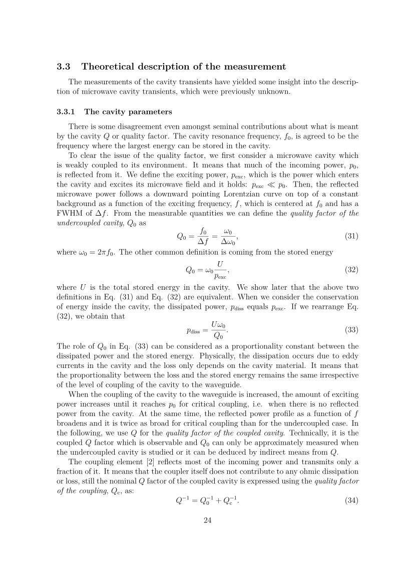
There is some disagreement even amongst seminal contributions about what is meantby the cavity Q or quality factor. The cavity resonance frequency, f0, is agreed to be thefrequency where the largest energy can be stored in the cavity.

To clear the issue of the quality factor, we first consider a microwave cavity whichis weakly coupled to its environment. It means that much of the incoming power, p0,is reflected from it. We define the exciting power, pexc, which is the power which entersthe cavity and excites its microwave field and it holds: pexc p0. Then, the reflectedmicrowave power follows a downward pointing Lorentzian curve on top of a constantbackground as a function of the exciting frequency, f , which is centered at f0 and has aFWHM of ∆f . From the measurable quantities we can define the quality factor of theundercoupled cavity, Q0 as

Q0 = f0

∆f = ω0

∆ω0, (31)

where ω0 = 2πf0. The other common definition is coming from the stored energy

Q0 = ω0U

pexc, (32)

where U is the total stored energy in the cavity. We show later that the above twodefinitions in Eq. (31) and Eq. (32) are equivalent. When we consider the conservationof energy inside the cavity, the dissipated power, pdiss equals pexc. If we rearrange Eq.(32), we obtain that

pdiss = Uω0

Q0. (33)

The role of Q0 in Eq. (33) can be considered as a proportionality constant between thedissipated power and the stored energy. Physically, the dissipation occurs due to eddycurrents in the cavity and the loss only depends on the cavity material. It means thatthe proportionality between the loss and the stored energy remains the same irrespectiveof the level of coupling of the cavity to the waveguide.

When the coupling of the cavity to the waveguide is increased, the amount of excitingpower increases until it reaches p0 for critical coupling, i.e. when there is no reflectedpower from the cavity. At the same time, the reflected power profile as a function of fbroadens and it is twice as broad for critical coupling than for the undercoupled case. Inthe following, we use Q for the quality factor of the coupled cavity. Technically, it is thecoupled Q factor which is observable and Q0 can only be approximately measured whenthe undercoupled cavity is studied or it can be deduced by indirect means from Q.

The coupling element [2] reflects most of the incoming power and transmits only afraction of it. It means that the coupler itself does not contribute to any ohmic dissipationor loss, still the nominal Q factor of the coupled cavity is expressed using the quality factorof the coupling, Qc, as:

Q−1 = Q−10 +Q−1

c . (34)

24

This also implies that Eq. (32) does not hold for the coupled Q, only for the under-coupled value. Eq. (34) explains that for critical coupling Q = Q0/2 as therein Qc = Q0.Clearly, the critical coupling is a distinguished case. We show below that this is not onlydue to the lack of power reflection but it also means that power dissipated inside thecavity equals the power transmitted through the coupling element.

Figure 20: Schematics of the iris of a cavity and the reflected, transmitted, and radiationemanating from the cavity.

Fig. 20. shows the schematics of the microwave cavity and the coupling element. Thecoupling element reflects R amount of the incoming power and transmits T portion ofit and R + T = 1. There are three microwave components which are to be considered:the microwave field that is reflected from the coupler, Erefl, the microwave field whichenters the cavity and excites it, Eexc, and the microwave field that emanates from thecavity through the coupler, Eem. It is the interference between the first and third termswhich results in zero reflected power from the cavity for critical coupling and irradiationfor f = f0 as these have opposite microwave phase [2]. Often, this interference effect isreferred to as microwave field reflected from the cavity. The thorough description of thisinterference effect is important for the cavity transient signals as the amount of reflectedpower depends on the state of the cavity [8].

Conservation of energy dictates that then pexc = p0 = pdiss. The energy accumulatedinside the cavity is then U = p0Q0/ω0, thus the emanated electric field is:

Eem =√Uω0T , (35)

whose magnitude equals that of the reflected electric field:

Erefl =√p0R. (36)

Eqs. (35) and (36) yield that

R = Q0

1 +Q0, (37)

T = 11 +Q0

. (38)

25

3.3.2 The switch off transient

We first consider a critically coupled cavity which is irradiated at its resonance fre-quency, f = f0, in its stationary state with energy U(t = 0) = U0 = p0Q0/ω0. The cavityloses energy through two paths after the excitation is switched off: by radiation throughthe coupling element and by dissipation. The corresponding differential equation for thestored energy U(t) reads:

dUdt = −pem − pdiss = −Uω0T −

Uω0

Q0. (39)

Which yields after rearranging:

dUdt = −Uω0

(1

1 +Q0+ 1Q0

)= −Uω0

Q. (40)

Where the quality factor of the coupled cavity is:

1Q

= 2Q0 + 1(1 +Q0)Q0

≈ 2Q0. (41)

The approximation is valid when Q0 1, which is often satisfied as Q values in excess of1.000 are customary. The solution for the critically coupled case and f = f0 thus reads:

U(t) = U0 e−ω0t

Q ≈ U0 e−2ω0t

Q0 . (42)

Using that pem = Uω0T we obtain Eqs. 5 and 6 for the power and the amplitude ofthe microwave voltage which is emitted from the cavity.

pem(t) = p0 e−ω0t

Q ≈ p0 e−2ω0t

Q0 , (43)

Vem(t) =√p0Z0 e−

ω0t

2Q ≈√p0Z0 e−

ω0t

Q0 , (44)

where Z0 is the wave impedance of the of the microwave waveguide.

3.3.3 The switch on transient

After switch on the energy balance of the cavity reads (for critical coupling and f = f0):

dUdt = pexc − pdiss, (45)

where pdiss = U ω0Q0

due to the arguments above. During the transient, the power reflectedfrom the cavity is not zero and thus the exciting power reads:

pexc = p0 − |Erefl − Eem|2 , (46)

which equals according to Eqs. (35) and (36):

pexc = p0 −∣∣∣∣√p0R−

√Uω0T

∣∣∣∣2 . (47)

26

Eq. (45) reads when Q0 1:

dUdt = 2

√p0Uω0

Q0− 2Uω0

Q0. (48)

It can be readily verified that the solution

U(t) = p0Q0

ω0

(1− e−

ω0t

Q0

)2, (49)

satisfies the starting conditions and the differential equation. The power which is reflectedfrom the cavity during the transient is obtained as:∣∣∣∣∣√p0 −

√Uω0

Q0

∣∣∣∣∣2

= p0 e−2ω0t

Q0 , (50)

and the corresponding amplitude of the microwave voltage reads:√p0Z0 e−

ω0t

Q0 . Theseresults are identical to that in Eq. (44). It also confirms that Eqs. 5 and 6 are valid forboth the switch on and off transients.

Finally, we note that often a relaxation time is defined to describe the cavity transient[2]. It is however misleading as one has to specify whether the relaxation time is referredfor the microwave voltage (measured using a mixer) or microwave power (measured usinga power detector).

3.3.4 Transients for arbitrary coupling

Herein, the case of non-critical coupling is considered for irradiation at resonance, i.e.f = f0. The exciting power inside the cavity, pexc is not necessarily p0, and there is a finitereflected power even in the steady state. To describe this situation, the β = Q0

Qcfactor is

introduced. As a result, for arbitrary coupling the cavity Q factor reads Q = Q0/(1 + β).The power exciting the cavity is:

pexc = p04β

(1 + β)2 (51)

and the power reflected from the cavity is p0 − pexc. It can be readily shown using theconservation of energy that the microwave power leaving the cavity is βpexc as it satisfiesthe requirement:

(√p0 −

√βpexc

)2= p0 − pexc.

The differential equation for the energy stored inside the cavity reads for the switchoff transient:

dUdt = −(1 + β)pexc = −(1 + β)U ω0

Q0. (52)

This is solved with the U(t = 0) = U0 = pexcQ0/ω0 initial condition

U(t) = U0 e−(1+β) ω0t

Q0 = U0 e−ω0t

Q . (53)

The amplitude of the microwave voltage which is detected during the transient reads:

V (t) =√pexcZ0β e−

ω0t

2Q = 2β1 + β

√p0Z0 e−

ω0t

2Q . (54)

27

Considering the switch on transient yields the same result for the power and microwavevoltage amplitudes which are reflected from the cavity. Clearly, the Fourier transformanalysis of Eq. (54) yields a Lorentzian in frequency space which corresponds to thequality factor of Q and it is therefore the generalization of Eqs. 5 and 6.

3.4 Time-domain cavity transientsUsing the previously shown experimental setup, several measurements of microwave

resonator transients were made. Figure 22 shows the typical switch-on and switch-offtransient measurements. Since the DC level of the switch-off transient is zero for both thecritically coupled and undercoupled case, the measurements of the switch-off transient ismore practical.

See figure 21 for cavity transients of two different cavities.

Figure 21: Comparison of the on-resonance transients for different quality factors.

28

Figure 22: Time-domain signals shown for critical and undercoupled cases. For the latter,half of the exciting power is reflected from the cavity when the irradiation is on resonanceand the steady state is achieved.

29

3.4.1 Analysis in the time-domain

One of the largest difficulties is the time it takes to transfer data on the relativelyslow GPIB protocol between the oscilloscope and the computer. The characteristic timeof the cavity transient is about 1 μs. The chopping frequency can be increased to about300 kHz. Transfering the data of one curve pair takes about 1 s. This means that we onlymeasure 1 in every 3 · 105 ringdown with high resolution. The high resolution means thatseveral data points have to be measured, which require a long data transfer time. Alsothe numerical fitting of the theoretical curve to the measured curve takes a significantamount of time.

The measurements were made using a Lecroy LT342 oscilloscope. This scope has a”sequence” working mode, which means that the scope measures after each trigger withlower resolution but averages several of these curves. The upper limit on the scope isaveraging 1000 transients, each consisting of 50 points. As there are much fewer pointsthat need to be transferred to the computer due to the low resolution, each curve takesonly 0.2 s to measure and transfer to the computer.

1000curves0.2 s = 5 kHz (55)

This means that every 1 in 60 curves can be measured. By decreasing the resolutionof each curve, the fitting time also decreases. The fitting on our setup took an additional0.2 s.

To check the performance of this method, 100 curves were collected, which took 20 s(1 curve is obtained by averaging 1000 curves), and fitted them in an addtitional 20 s, soone measurement took 0.4 s. See figure 23 for a typical measured curve.

τ = 1.4131 μs± 0.971 ns (56)Q = 2πfresτ/2 = 48593 (57)S

N= 1454√

0.4 s= 2299

√Hz (58)

Figure 23: A measured curve, and fit.

30

3.4.2 Analysis in the frequency-domain

As discussed above, the Fourier transform power spectrum of the IQ mixer outputsdirectly yields the cavity resonance curve. To experimentally verify this statement, ameasurement was made where the source frequency was 20 MHz off-resonance. In Fig.24 the Fourier tramsform of the mixer outputs is presented. In Fig. 25 the Fourier poweris presented.

Figure 24: The Fourier transformed signal for a measurement 20 MHz off-resonance

For this method the best measurement setup was achieved by using high resolutionand average several curves using the oscilloscope. This means that transferring the mea-surement data to the scope took relatively little time.

This method can be used to measure the resonance frequency and Q simultaneously,while being further off-resonance than using the analysis in the time-domain. The reasonfor this observation is that the time-domain analysis method uses low resolution, so wecannot observe the exponential decay and the beat frequency at the same time.

Analysis in the frequency domain gives a smaller signal to noise ratio than the analysisin the time domain. This is due to the fact, that more points have to be transferred fora good FT spectrum, and the processing of the FT and the fitting of the Lorentzian alsotakes more time.

3.4.3 Effect of significant detuning

To check the off-resonance perfprmance of the technique, measurements were madeusing the FT method. Using this method we can measure the frequency and power ofthe energy of the transient. The energy emitted from the cavity is obtained from the

31

Figure 25: FT power for a measurement 20 MHz off-resonance

integrated intensity of the FT signal as a function of f − f0.

Uem = p0Q0∆ω2

2ω0(∆ω2 + (ω − ω0)2

) . (59)

These measurements have shown that the off-resonance operation of the method isfairly well understood. The deviation from the calculated values is shown in figure 26.We obtain a good agreement between the measured and calculated values for the emittedenergy with a small deviation for significant detuning. We believe that this deviation isdue to the frequency dependent properties of the microwave components.

32

a)

FT p

ower

(ar

b. u

.)

+ 20 MHzx200

-100 MHzx40,000

-100 -50 0 50 100

b)

Em

itted

ene

rgy

(J)

f-f0 (MHz)

10-14

10-12

10-10

Figure 26: a) FT data for different values of f − f0 (from top to bottom): 0, +20 MHz,and -100 MHz. Note the different vertical scales, the DC peak for the +20 MHz data,and that this range is not shown for the -100 MHz data. b) The energy emitted from thecavity versus the exciting frequency. The solid curve is the calculated values, the symbolsare data obtained from the emitted signal..

33

3.5 Performance of the novel method

Method Q t [sec] δ (Q) δ (f0)Stepped frequency sweep Ref. [5] 108 − 109 10 6 · 10−4 6 · 10−4

AFC based method Ref. [3] 2.5 · 104 3 10−3 10−3

Present method 104 − 105 1 10−3 10−3

Table 1: Comparison of the different Q and f0 measurement methods (t denotes themeasurement time).

Herein, we compare the performance of methods, which are found in the literature,with the present one. We use the quantities for the error of Q and f0 as defined in section3.4.1. We find that the present method has similar error for a similar measurementtime. The present method is limited for Q > 1000 values due to the available timeresolution and PIN diode switching speed. However, we expect it to perform better thanthe conventional methods for higher Q values (even up to theQ = 109 range) as therein thelimiting factors are the measurement speed where the present method with its multiplexadvantage is a true asset. This is very similar to the multiplex advantage which motivatedthe development of the pulsed NMR technique. The absolute accuracy of both and f0and Q is traced back to the accuracy of the local oscillator, which can be very high withthe use of atomic clocks referencing. This is essentially the so-called Connes (accuracy)advantage [9] of the FT based techniques.

Another advantage of the present method is its ability to measure dynamics of mi-crowave absorption inside microwave cavities. Effects like sample heating [10] are knownto affect the microwave cavity parameters during a measurement. The conventional meth-ods are limited to few ms-s measurement time, whereas for the present one, the only timelimit is the cavity transient time itself.

34

4 SummaryIn this thesis we presented a novel method for the measurement of the quality factor

of microwave resonators. We showed the issues of the traditional methods, namely theunstable nature of the frequency sweeps used. The novel method is based on measuringthe resonator transient and so has several advantages over the traditional methods:

• faster measurement than most traditional methods

• less prior knowledge necessary of the resonance frequency of the resonator

• easy measurement of high-Q systems

while maintaining a similar signal-to-noise ratio.We made measurements using an NMR console to highlight the similarities of mi-

crowave and RF system. We also made measurements on microwave cavities with Qbeing apprixomately 10,000 50,000 to check the performance of the new method.

We presented the theoretical description of the resonator transient, which proved tobetter suit the measurements than the ones found in the literature. We presented asuggestion for a figure of merit for microwave cavity measurements and compared themethods found in sthe literature based on it.

35

References[1] M Dressel, O Klein, S Donovan, and G Gruner. Microwave cavity perturbation

technique: Part 3: Applications. International Journal of Infrared and MillimeterWaves, 14(12):2489–2517, 1993.

[2] C. P. Poole. Electron Spin Resonance: A Comprehensive Treatise on ExperimentalTechniques. Dover Books on Physics. Dover Publications, 1996.

[3] B. Nebendahl, D. N. Peligrad, M. Pozek, A. Dulcic, and M. Mehring. An ac methodfor the precise measurement of q-factor and resonance frequency of a microwavecavity. Review of Scientific Instruments, 72(3):1876–1881, MAR 2001.

[4] Andre Luiten. Q-Factor Measurements. John Wiley & Sons, Inc., 2005.

[5] A. N. Luiten, A. G. Mann, and D. G. Blair. High-resolution measurement of thetemperature-dependence of the q, coupling and resonant frequency of a microwaveresonator. Measurement Science & Technology, 7(6):949–953, JUN 1996.

[6] P. J. Petersan and S. M. Anlage. Measurement of resonant frequency and qualityfactor of microwave resonators: Comparison of methods. Journal of Applied Physics,84(6):3392–3402, SEP 15 1998.

[7] http://cas.web.cern.ch/cas/Denmark 2010/Caspers/Skyworks-SchottkyDiodes-Basics

[8] W.J. Gallagher. Transient-response of a microwave cavity. IEEE Transactions onNuclear Science, 26(3):4277–4279, 1979.

[9] Janine Connes and Pierre Connes. Near-Infrared Planetary Spectra by Fourier Spec-troscopy.I. Instruments and Results. J. Opt. Soc. Am., 56(7:896-910), 1966.

[10] Anita Karsa, Dario Quintavalle, Laszlo Forro, and Ferenc Simon. On the low temper-ature microwave absorption anomaly in single-wall carbon nanotubes. physica statussolidi (b), 249(12):2487–2490, 2012.

[11] C. G. Montgomery, R. H. Dicke, and E. M. Purcell. Principles of Microwave Circuits.McGraw-Hill Book Company, Inc., New York, United States, 1948.

36

AppendixA The transients in an equivalent circuit model

This calculation presented herein was made by Bence Markus and is given in this thesisfor the sake of completeness. During the previous considerations the f = f0 on resonancecase was discussed, where we took in the conservation of energy and wave interferenceeffects. For the general, f 6= f0 case a lumped circuit equivalent of the coupled microwavecavity has to be taken in account. The lumped circuit equivalent of an iris-coupled cavityaccording to [11] is shown on Fig. 27. for arbitrary Q and Fig. 28. for high-Q, with thepresumption of L L.

R

C

L

L

Figure 27: Equivalent RLC-circuit of acoupled cavity [11] near resonance.

ω2L2/Z

0

Figure 28: Equivalent RLC-circuit of acoupled high-Q cavity [11] near resonance.

The integro-differential equation for the discharge transient according to Ohm’s law:

0 = 1C

∫I dt+ (L+ L)dI

dt +(R + ω2L2

Z0

)I, (60)

After differentiating a second order differential equation can be obtained:

0 = I

C+ (L+ L)d2I

dt2 +(R + ω2L2

Z0

)dIdt . (61)

Using the I(t) = A e−λt ansatz the characteristic equation near resonance:

λ1,2 =R + ω2

0L2

Z0

2(L+ L) ± i

√√√√√R + ω20L2

Z0

2(L+ L)

2

− 1C(L+ L) . (62)

Here the critical coupling can be achieved when

L2ω20 = Z0R. (63)

37

Using

ω0 = 1√C(L+ L)

, (64)

ω0

Q0= R

L+ L , (65)

ω0

Qc= ω2

0L2

Z0(L+ L) , (66)

Q−1 = Q−10 +Q−1

c , (67)Q = Q0/(1 + β), (68)

the Eq. (62) becomes

λ1,2 = ω0

2Q ± i

√√√√ω20 −

(ω0

2Q

)2

. (69)

The general solution for the discharge transient

I(t) =2∑i=1

Ai e−λit, (70)

where the Ai coefficients must be fitted to satisfy the initial state conditions. Here it hasto be emphasized that according to Eq. (69) the transient always has a characteristicdecay rate of ω0/2Q, which is in an agreement with the previous calculations and withEqs. 5 and 6. However the oscillating part does not exactly equal this, this is because ofthe damping, which causes a small shift in the resonance frequency.

During the turn on transient similar considerations have to be made. In this case thecharacteristic exponent remains the same as the one in Eq. (69).

38

B Additional methods consideredIn the process of understanding the cavity transients and deciding how to best make use

of them in measuring the quality factor, other measurement techniques were considered

B.1 High frequency sweepThe frequency sweeping method can be improved by high frequency chopping of the

signal, i.e. amplitude modulating the output of the source with a rectangular wave. Thefrequency components in the chopping rectangular signal are mixed with the microwavefrequency. This gives rise to sidebands. The distance of the first sidebands from theresonance frequency is the chopping frequency. As stated before, one of the major errorsof the frequency sweeping measurements is that the frequency sweep is not reproducible,i.e. the frequency axis is not calibrated. As we know the chopping frequency quite well,we can use the sidebands to calibrate the frequency axis.

Figure 29: Measurement made by using 2 MHz chopping for a cavity with a bandwidthof 1.5 MHz.

While this method proved to be effective, it did not improve the measurement bymuch, so generally it is not worth the additional difficulty of using a fast PIN diode andfunction generator.

39

B.2 Lock-in quadrature detectionIn this method, the microwave power is chopped with a rectangular signal using a

PIN diode. We can measure the reflection or transmission of the signal using a Lock-inamplifier. If the cavity did not have a switching transient, the measured signal would onlyconsist of an in-phase signal. This is only true if we take the delays of the system intoaccount. Due to the transient, the signal leaks into the quadrature as seen in figure 30.In principle the Q would be obtained from the phase of the lock-in. While the method isfeasible, it did not turn out to be a practical one: first, the accurate measurement of thephase requires a calibration since there are several sources (e.g. finite singal propagationtime) which can cause a phase shift. Secondly, the relative noise of the phase can beshown to be relatively large.

Figure 30: Schematics of the quadrature and cavity signal.

40

B.3 Lock-in higher harmonicsIn this method, the microwave power is chopped with a rectangular signal using a PIN

diode. We can measure the reflection or transmission of the signal using a power detectorand a Lock-in amplifier. When using a power detector, the transients have the same sign,so if the cavity did not have a switching transient, the measured signal would not have asecond harmonic signal. Due to the transient, we may observe a second harmonic signalas seen in figure 31.

Figure 31: Schematics of the 2nd harmonic and cavity signal.

41

C Measurements on a superconducting microwavecavity

C.1 Construction of the superconducting cavityMeasuring cavities with high quality factors may be exceedingly difficult by frequency

sweeping methods, because the frequency instability becomes relatively larger in compar-ison to the resonance’s width. Due to this, our problem is even more analogous to theNMR. Cavities with large Q can be used to measure samples of very small size, thesecavities are made of superconductive materials and are cooled below their critical tem-peratures.A cavity made of niobium was built to demonstrate the time-domain method on a rela-tively large Q factor. Niobium is a superconductor, its critical temperature is 9.2 K. Theshape and size of the cavity is the same as an already existing cavity, which is used forlow temperature measurements, so the cooling was achievable easily using its cryogenicprobehead.

Figure 32: Photograph of the niobium cavity when assembled on the cryogenic probehead.

The cryogenic probehead was slightly modified to increase the quality factor and cancelheat bridges between the cavity and room temperature.

The quality factor of the coupling to the cavity was measured to make sure, that thequality factor of the system is dominated by the cavity. The method to measure thecoupling is described in my BSc thesis, and will not be described in detail here. Thequality factor of the coupling 200,000, so as long as the quality factor of the system issignificantly smaller, it is dominated by the cavity.After construction, the niobium cavity was cleaned in an acetone bath by ultrasoundcleaner, then baked at 200 C for about 10 minutes in argon enviroment. Accordingto the literature, this method removes the O2 and N2 contamination absorbed into the

42

niobium crystal lattice.The highest achieved quality factor in the niobium cavity was about 50000, its reso-

nance frequency is 10.96 GHz, its bandwidth is 0.2 MHz.

C.2 Measurements on the superconducting cavity

Figure 33: Measured transient of the superconducting cavity.

Measurements of the new cavity were made using the new method and found that itsquality factor is 48,600.

The new method was tested on a regular cavity Q = 10, 000 and this high Q cavity.Similar signal to noise ratios were found.

The quality factor of the newly built niobium cavity was measured, while it was slowlywarmed from the lowest achievable temperature. The thermometer was very close to theheater circuit in the cavity, so it is probable that most of the cavity was significantlycolder than the measured temperature. This may account for the slow change in the Q,instead of the sudden drop at the critical temperature. We seemingly measure that thechange to superconductive phase starts at 20 K, but the explanation for this is that thethermometer was not completely thermalized to the cavity.

43

Figure 34: The quality factor of the cavity as a function of the temperature for increasingtemperature.

44