multi period financial planning

8/3/2019 Multi Period Financial Planning

http://slidepdf.com/reader/full/multi-period-financial-planning 1/12

D.-S. Huang, K. Li, and G.W. Irwin (Eds.): ICIC 2006, LNAI 4114, pp. 1158 – 1169, 2006.

© Springer-Verlag Berlin Heidelberg 2006

Solving Multi-period Financial Planning Problem Via

Quantum-Behaved Particle Swarm Algorithm

Jun Sun, Wenbo Xu, and Wei Fang

Center of Intelligent and High Performance Computing,

School of Information Technology, Southern Yangtze University,

No. 1800, Lihudadao Road, Wuxi,

214122 Jiangsu, China{sunjun_wx, xwb_sytu, wxfangwei}@hotmail.com

Abstract. A multistage stochastic financial optimization manages portfolio in

constantly changing financial markets by periodically rebalancing the asset

portfolio to achieve return maximization and/or risk minimization. In this paper,

we present a decision-making process that uses our proposed Quantum-behaved

Particle Swarm Optimization (QPSO) Algorithm to solve multi-stage portfolio

optimization problem. The objective function is classical return-variance func-

tion. The performance of our algorithm is demonstrated by optimizing the allo-

cation of cash and various stocks in S&P 100 index. Experiments are conducted

to compare performance of the portfolios optimized by different objective func-

tions with Particle Swarm Optimization (PSO) algorithm and Genetic Algo-

rithm (GA) in terms of efficient frontiers.

1 Introduction

Financial optimization involves asset allocation and risk management. A multi-stage

stochastic financial optimization is a quantitative model that integrates asset alloca-

tion strategies and saving strategies in a comprehensive fashion. It manages portfolio

in constantly changing financial markets by periodically rebalancing the asset portfo-

lio to achieve return maximization and risk minimization. Stochastic optimization of

portfolio is NP-hard and is non-linear with many local optima.

A number of different algorithmic approaches have been proposed for solving sto-

chastic optimization problems. To solve the asset allocation problem, one may em-

ploy linear programming solvers such as CPLEX and OSL by piecewise linearizing

the nonlinear objective function [2]. The interior-point algorithms are another type of

methods well suited to the scenario structure of multi-stage stochastic programs.

Searching the global solution by these methods, however, is computationally expen-

sive and ineffectively. Since time is a constraint for financial problems, a trade-off

should be made between the performance and the computational time. Heuristic meth-ods, such as Tabu Search [1] and GA [3] provide some appropriate ways to find opti-

mal asset allocation.

Particle Swarm Optimization (PSO) was originally proposed by J. Kennedy as a

simulation of social behavior of bird flock, and was initially introduced as a heuristic

optimization method in 1995 [7]. More recently, a new version of PSO, called



Solving Multi-period Financial Planning Problem 1159

Quantum-behaved Particle Swarm Optimization (QPSO), has been proposed in order

to improve the global search performance of the original PSO [12], [13], [14]. The

QPSO is a global convergent and has fewer parameters to control, which makes it

easier to implement.

In this paper, we explore the practicability of QPSO in multi-stage financial opti-mization problem. To do so, we used S&P 100 Index and the prices of its component

stocks as the training samples. The PSO and GA were also tested on the sample data

for performance comparison. The rest of the paper is organized as follows. In next

section, the multi-stage portfolio optimization model is described. In Section 3 and

Section 4, we describe the PSO and QPSO in detail. Section 5 is the presentation of

experiment results and the paper is concluded in Section 6.

2 Multi-stage Portfolio Optimization Model

Single period portfolio optimization model possesses several drawbacks. For exam-

ples, the risk is inconsistent over time. The multi-stage stochastic programming model

proposed by Mulvey et al [8], [9] captures dynamic aspects of asset allocation prob-

lem. It manages portfolio in constantly changing financial markets by periodically

rebalancing the asset portfolio to achieve return maximization and/or risk minimiza-

tion, leading to optimal portfolio.

To define the model, we divide the entire planning horizon T into two discrete in-

tervals1T and

2T , where τ ,,1,01 L=T and T T ,,12 L+= τ . The former corre-

sponds to periods in which investment decisions are made. Period τ defines the date

of planning horizon; we focus on the investor’s position at the beginning of period τ.

Decisions occur at the beginning of each time stage.2T handles the horizon at time τ

by calculating economic and other factors beyond period τ up to period T. The inves-

tor cannot render any active decisions after the end of period τ.

Asset investment categories are defined by set I A ,,2,1 L= , with category 1

representing cash. The remaining categories can include broad investment groupings

such as stocks, bonds, and real estate. Ideally, the co-movements between pairs of

asset returns would be relatively low so that diversification can be done across theasset categories. In the model, uncertainty is modeled through a large but finite num-

ber S of scenarios. Each scenario represents a possible realization of all uncertain

parameters in the mode. To be specific, let t ω represent the vector of random pa-

rameters whose values are revealed in period t. Then the set of all scenarios is the set

of all realizations { }SSssss ,,2,1:),,,,( 21 LL =∈τ ω ω ω , of ),,,( 21 τ ω ω ω L .

Each scenario s has a probability sπ , where 0>sπ and 1

1=∑ =

S

s sπ . Since in a

dynamic model information on actual value of the uncertain parameters is revealed in

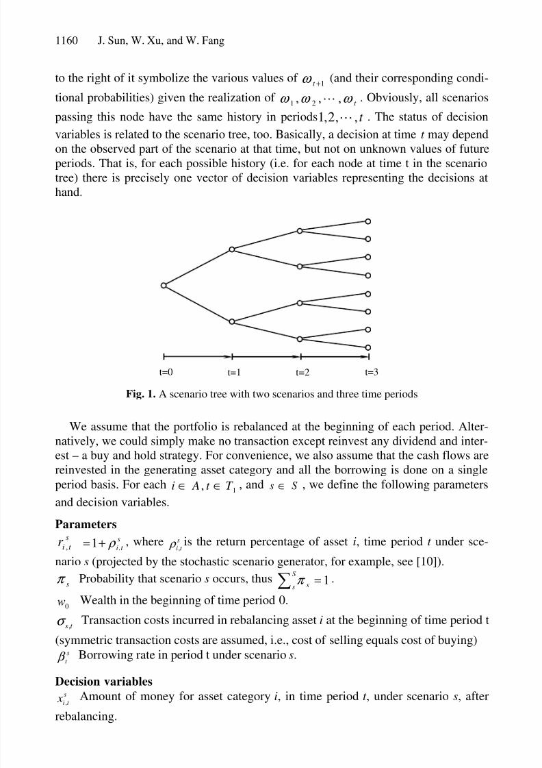
stages, a suitable representation of scenarios is given by a scenarios tree, such as in

Figure 1. In this case τ =3 and S=8. Each path form t=0 to t=τ represents one scenario.

Any node of the tree, corresponding to time t , symbolizes a possible state of the world

at time t, represented by the observed values of t ω ω ω ,,, 21 L . The branches directly



1160 J. Sun, W. Xu, and W. Fang

to the right of it symbolize the various values of 1+t ω (and their corresponding condi-

tional probabilities) given the realization of t ω ω ω ,,, 21 L . Obviously, all scenarios

passing this node have the same history in periods t ,,2,1 L . The status of decision

variables is related to the scenario tree, too. Basically, a decision at time t may dependon the observed part of the scenario at that time, but not on unknown values of future

periods. That is, for each possible history (i.e. for each node at time t in the scenario

tree) there is precisely one vector of decision variables representing the decisions at

hand.

t=0 t=1 t=2 t=3

Fig. 1. A scenario tree with two scenarios and three time periods

We assume that the portfolio is rebalanced at the beginning of each period. Alter-

natively, we could simply make no transaction except reinvest any dividend and inter-

est – a buy and hold strategy. For convenience, we also assume that the cash flows are

reinvested in the generating asset category and all the borrowing is done on a single

period basis. For each1, T t Ai ∈∈ , and Ss ∈ , we define the following parameters

and decision variables.

Parameters

st ir , s

t i,1 ρ += , where st i, ρ is the return percentage of asset i, time period t under sce-

nario s (projected by the stochastic scenario generator, for example, see [10]).

sπ Probability that scenario s occurs, thus 1=∑S

s sπ .

0w Wealth in the beginning of time period 0.

t s,σ Transaction costs incurred in rebalancing asset i at the beginning of time period t

(symmetric transaction costs are assumed, i.e., cost of selling equals cost of buying)s

t β Borrowing rate in period t under scenario s.

Decision variabless

t i x ,Amount of money for asset category i, in time period t , under scenario s, after

rebalancing.




s

t iv ,Amount of money in asset category i, in the beginning of time period t , under

scenario s, before rebalancing.s

t w Wealth at the beginning of time period t , under scenario s.

st i p ,

Amount of asset i purchased for rebalancing at time t under scenario s.

s

t id , Amount of asset i sold for rebalancing in time period t , under scenario s.

s

t b Amount of money borrowed in period t , under scenario s.

Given these definitions, we outline the general stochastic programming model in

financial optimization.

Model SP

∑=

=S

s

s

s w f Z 1

)(Max τ π (1)

s.t.

∑ ∈∀=i

s

i Ssw x ,00,

(2)

,,2,1,, τ L=∈∀=∑ t Ssw xi

s

t

s

t i

(3)

,,,2,1,1,1,, Ait Ss xr vst

t i

s

t i

s

t i∈=∈∀= −− τ L (4)

1,,,2,1,)1( ,,,,, ≠=∈∀−−+= it Ssd pv x s

t it i

s

t i

s

t i

s

t i τ σ L (5)

,,,2,1,

)1()1( 11

1

,

1

,,,1,1

τ

β σ

L=∈∀

++−−−+= −−

≠≠

∑∑

t Ss

bb pd v xs

t

s

t

s

t

i

s

t i

i

t i

s

t i

s

t

s

t (6)

'

,,

s

t i

s

t i x x = for all scenarios s and s’ with identical past up to time t (7)

As with the single-period models, the nonlinear objective function (1) can take sev-

eral different forms. If the classical return-risk function is employed, then (1) be-

comes )Var()1()Mean(Max τ τ η η ww Z ⋅−−⋅= , where )Mean( τ w is the average

total wealth and )Var( τ w is the variance of the total wealth across the scenarios at the

end of period τ. Parameter η indicates the relative importance of variance as com-

pared with the expected value. This objective leads to an efficient frontier of wealth at

period τ.

Constraint (2) guarantees that the total initial investment equals the initial wealth.

Constraint (3) states the wealth accumulated at the end of t -th period under scenario s

before rebalancing in asset i. This constraint can be modified to include assets,




liabilities, and investment goals. Constraint (4) depicts the wealths

t iv , accumulated at

the beginning of period t before rebalancing in asset i. The flow balance constraint for

all assets except cash for all periods is given by constraint (5). This constraint guaran-

tees that the amount invested in period t equals the net wealth for asset. Constraint (6)represents flow balancing constraint for cash. Non-anticipativity constraint is repre-

sented by (7). These constraints ensure that the scenarios with the same past will have

identical decisions up to that period.

3 Particle Swarm Optimization

In a Particle Swarm Optimization (PSO) system, individuals representing the candi-

date solutions to the problem at hand fly through a multidimensional search space to

find out the optima or sub-optima. In PSO with M individuals, each individual istreated as a volume-less particle in the D-dimensional space, with the position vector

and velocity vector of particle i at k th iteration represented as

))(,),(),(()( 21 k X k X k X k X iDiii L= and ))(,),(),(()( 21 k V k V k V t V iDiii L= . The particles

move according to the following equations:

))()(())()(()()1( 2211 k X k Pr ck X k Pr ck V wk V ijgjijijijij ⋅⋅+−⋅⋅+⋅=+ (8)

)1()()1( ++=+ k V k X k X ijijij (9)

for D j M i ,2,1;,2,1 LL == . Parameters1

c and2

c are called acceleration coeffi-

cient. Vector ),,,( 21 iDiii PPPP L= is the best previous position (the position giv-

ing the best fitness value) of particle i called personal best position, and vector

),,,( 21 gDggg PPPP L= is the position of the best particle among all the particles in the

population and called global best position. The parameters 1r and 2r are random

numbers distributed uniformly in (0,1). Generally, the value of Vid is restricted in the

interval],[ maxmax V V −

. The inertia weight w in equation (8) was introduced by Shi

and Eberhart [13]. The addition of the inertia weight results in faster convergence.

4 Quantum-Behaved Particle Swarm Optimization

Trajectory analyses in [5] demonstrated the fact that convergence of the PSO algo-

rithm may be achieved if each particle converges to its local attractor. Let the local

attractor ),,( 21 iDiii p p p p L= of particle i be defined at the coordinates

)(),()1()()( 221111 r cr cr cwherek Pk Pk p gjijij +=⋅−+⋅= ϕ ϕ ϕ (10)

with regard to the random numbers 1r and 2r in equation (8). It can be seen that the

local attractor is a stochastic attractor of particle i that lies in a hyper-rectangle with

iP and

gP being two ends of its diagonal and moves following

iP and

gP .




endif

endfor

endwhile

Generally, the value of α no more than 1.0 can lead to a good performance if it isfixed over the running of QPSO. But in most cases, α decrease linearly from 0α to

1α .

5 Numerical Experiments

In order to evaluate the performance of QPSO on multistage financial optimization,

experiments were carried out. Weekly closing prices of S&P 100 Index and its com-

ponent stocks from 1 January 2000 to 31 December 2004 were collected. Cash and

stocks of ten corporations that belong to different industries were selected to be opti-

mized. The planning horizon interval1T was divided into three periods.

In our approach, the economic parameter that determines scenarios is the mark in-

dex and therefore each scenario represents a possible realization of market index. We

set the market index two possible realization:(1) the market index has been raised and

(2) the market index has been dropped. Denoting rise with 1 and drop with 0, we can

obtain the scenario tree as Figure 1 with 8 scenarios: (0,0,0), (0,0,1), (0,1,0), (0,1,1),

(1,0,0), (1,0,1), (1,1,0) and (1,1,1). Each edge in the scenario tree corresponds to a

realization of market index’s raise and drop as well as a set of percentage returns of

all assets in time period t under a certain scenario. We worked outsπ of each scenario

and s

t i , ρ of each stock according to closing price of the index and stocks. For the per-

centage return of cash, we set a fixed annual interest rate 6%, and therefore the

weekly percentage return is 0.12% across the whole period of planning.

Usingsπ and s

t i, ρ as parameters, we tested three optimizers: QPSO, PSO and GA,

to search the optimal s

t i x ,to maximize the objective function (1). To implement the

algorithms, we adopted st ia , , allocation proportion of the selected assets after rebalanc-

ing under different scenarios over the planning horizon as our decision variables.

Therefore, s

t i x ,is determined by s

t

s

t i

s

t i wa x ⋅= ,,.

There are 15 nodes in the scenario tree with each node containing the allocation

proportions of 11 assets under the corresponding scenario. For each scenario s at time

t , the total asset allocation proportion must be equal to 100%. Hence, each of asset

allocation proportions

t ia , under scenario is normalized by ∑ ==

A

i

s

t i

s

t i

s

t i aaa1 ,

,

,

,

,,

after the optimization algorithm has run for an iteration, where

,

,

s

t ia is the normalizedasset allocation proportion. Moreover, in our numerical experiment, we don’t take

borrowing and transaction costs into account. The values of t s,σ , s

t β and s

t b in con-

straint (5), (6) are zeros consequently.




We employed the classical return-risk function as the objective function. Therefore

the purpose of our experiment was to generate an efficient frontier of wealth at

period τ. In order to generate the entire efficient frontier, we adopt a series of different

values of η in interval [0,1]. Some of these values of η are listed in the first column of

Table 4. Each objective function corresponding to a particular η was maximized togenerate a couple of Expected Return and Variance at period τ. Thus, a series Ex-

pected Return-Variance can be obtained to yield a curve of the efficient frontier.

Three groups of experiments were implemented with each group running an opti-

mization algorithm. The configurations of the three algorithms are as follows. For the

QPSO, the CE Coefficient was varying linearly from 1.0 to 0.5 over 500 iterations for

a running of the algorithm. The objective function corresponding to each vale of

η was maximized for 10 runs by the QPSO. For the experiment performed by the

PSO, the acceleration coefficients c1 and c2 in are set to be 2 keeping constant and the

inertia weight w was decreasing from 0.9 to 0.4 over 500 iterations for a running asadopted in most existing literatures. Also each objective function was optimized for

10 runs. Sixty particles were used in both the QPSO and PSO. For the GA, 100 indi-

viduals were employed. Each objective function was also maximized for 10 runs with

each run executed for 500 iterations too. The experiments of GA were performed

using real-valued encoding, binary tournament selection. Probability of mutating a

genome is 2.0=m p , and probability of crossover is 9.0=c p . The algorithm use a

arithmetic crossover with one weight for each variable. All weights exept one are

randomly assigned to either to 0 or 1. The other ones are set to a random number

between 0 and 1. This crossover operator is hybrid between uniform and arithmetic

crossover and showed a better performance than traditional uniform and arithmetic

crossover [15]. The mutation operator used here is standard Gaussian mutation with

zero mean and variance 112 += k σ , where k is iteration number.The search scope

for every decision variable is [0,1] for all experiments. At an iteration during execu-

ting the algorithm, if the allocation proportions of all assets at time t under scenario s

were all be zeros, the allcotion proportion of cash would be set to 1 to satisfy the

normalization ceriterion.

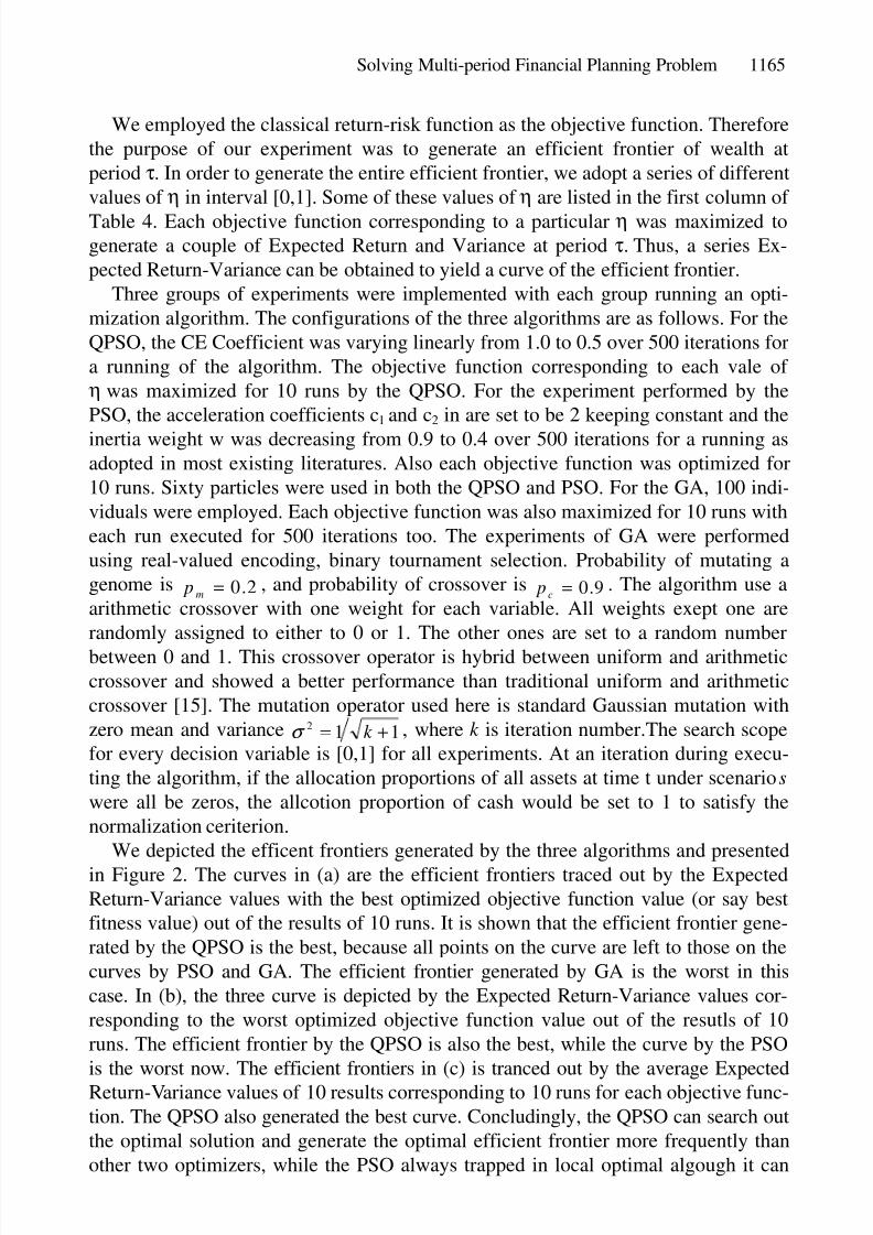
We depicted the efficent frontiers generated by the three algorithms and presented

in Figure 2. The curves in (a) are the efficient frontiers traced out by the Expected

Return-Variance values with the best optimized objective function value (or say best

fitness value) out of the results of 10 runs. It is shown that the efficient frontier gene-

rated by the QPSO is the best, because all points on the curve are left to those on the

curves by PSO and GA. The efficient frontier generated by GA is the worst in this

case. In (b), the three curve is depicted by the Expected Return-Variance values cor-

responding to the worst optimized objective function value out of the resutls of 10

runs. The efficient frontier by the QPSO is also the best, while the curve by the PSO

is the worst now. The efficient frontiers in (c) is tranced out by the average Expected

Return-Variance values of 10 results corresponding to 10 runs for each objective func-

tion. The QPSO also generated the best curve. Concludingly, the QPSO can search out

the optimal solution and generate the optimal efficient frontier more frequently than

other two optimizers, while the PSO always trapped in local optimal algough it can




0 2 4 6 8 100.02

0.021

0.022

0.023

0.024

0.025

0.026

0.027

Variance

P r o f i t

QPSO

GA

PSO

0 1 2 3 4 5 6 7 8 9 10-0.03

-0.02

-0.01

0

0.01

0.02

0.03

Variance

P r o f i t

QPSO

GA

PSO

(a) (b)

0 2 4 6 8 100

0.005

0.01

0.015

0.02

0.025

0.03

Variance

P r o f i t

QPSO

PSO

GA

(c)

Fig. 2. (a) Efficient frontiers generated by the best solutions out of 10 runs. (b). Efficient fron-

tiers generated by the worst solutions out of 10 runs. (c) Those generated by mean of solutions.

Table 1. Numerical results with some different values of η

QPSO GA PSO

η Max. Mean St. Dev. Max. Mean St.Dev Max. Mean St.Dev.

0.01 1.0037 1.0037 0.00007 0.9839 0.9803 0.0018 1.0036 0.8864 0.1336

0.2 20.1199 20.1198 0.00003 20.0635 20.0332 0.024 20.11 19.9772 0.1366

0.4 40.3817 40.3817 0.00006 40.3237 40.298 0.0172 40.3538 40.1117 0.2095

0.6 60.8801 60.88 0.00016 60.8199 60.7798 0.0317 60.7852 60.5629 0.1985

0.8 81.6346 81.6346 0.00000 81.5505 81.4797 0.0427 81.6346 81.3659 0.2004

1.0 102.664 102.664 0.00000 102.552 102.479 0.0372 102.664 102.299 0.3996

find out the global opima occasionally. The fact that the performance of the GA is

inferior to that of the QPSO is due to its slow convergence rate, which can be seen in

the following part of the paper.




0 100 200 300 400 5006.5

7

7.5

8

8.5

9

9.5

10

10.5

Iteration

M e a n F i t n e s

s

QPSO

PSO

GA

0 100 200 300 400 50037

37.5

38

38.5

39

39.5

40

40.5

Iteration

M e a n F i t n e s s

QPSO

PSO

GA

(a) (b)

0 100 200 300 400 500

67.5

68

68.5

69

69.5

70

70.5

71

71.5

Iteration


QPSO

PSO

GA

0 100 200 300 400 50088

88.5

89

89.5

90

90.5

91

91.5

92

92.5

Iteration


QPSO

PSO

GA

(c) (d)

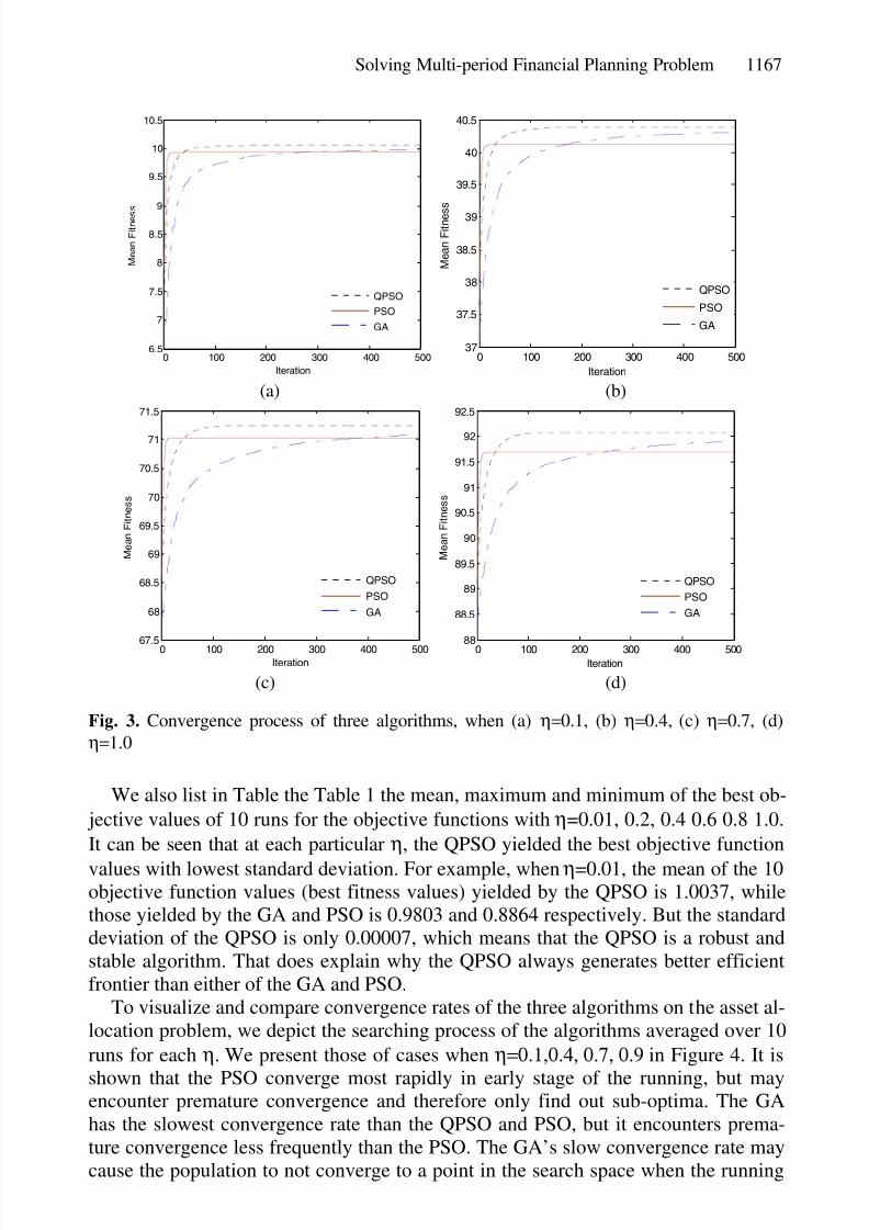
Fig. 3. Convergence process of three algorithms, when (a) η=0.1, (b) η=0.4, (c) η=0.7, (d)

η=1.0

We also list in Table the Table 1 the mean, maximum and minimum of the best ob-

jective values of 10 runs for the objective functions with η=0.01, 0.2, 0.4 0.6 0.8 1.0.

It can be seen that at each particular η, the QPSO yielded the best objective function

values with lowest standard deviation. For example, when η=0.01, the mean of the 10objective function values (best fitness values) yielded by the QPSO is 1.0037, while

those yielded by the GA and PSO is 0.9803 and 0.8864 respectively. But the standard

deviation of the QPSO is only 0.00007, which means that the QPSO is a robust and

stable algorithm. That does explain why the QPSO always generates better efficient

frontier than either of the GA and PSO.

To visualize and compare convergence rates of the three algorithms on the asset al-

location problem, we depict the searching process of the algorithms averaged over 10

runs for each η. We present those of cases when η=0.1,0.4, 0.7, 0.9 in Figure 4. It is

shown that the PSO converge most rapidly in early stage of the running, but mayencounter premature convergence and therefore only find out sub-optima. The GA

has the slowest convergence rate than the QPSO and PSO, but it encounters prema-

ture convergence less frequently than the PSO. The GA’s slow convergence rate may

cause the population to not converge to a point in the search space when the running




is over. Comparing with the other two algorithms, the QPSO can converge rapidly

and search out the global optima most frequently.

Although the PSO is invented to solve GO problems, it is not a global convergence

guaranteed algorithm. If the particles in the PSO trap into sub-optima, they have less

possibility to skip out, particularly in the late stage of the running. The GA is globalconvergent, but its convergence rate are so slow that its local search ability in late

stage of running is weakened. The QPSO not only possess, rapid convergence rate,

the strongpoint of the PSO, but it is guaranteed to be global convergent, which makes

it outperform the PSO and GA in our tested portfolio optimization problem. In fact,

not only the portfolio optimization problem is the QPSO excellent in, but it superior

to the PSO and GA in other function optimization problems also [14].

6 Conclusions

In this paper, QPSO algorithm is used to optimize a multi-stage portfolio. The objec-

tive function used is classical expected return-variance function with S&P 100 index,

cash and 10 selected component stock been optimized. Comparing with PSO and GA,

QPSO generate better efficient frontiers with better objective function value and ro-

bustness. Furthermore, the convergence rates of the algorithms was studied and the

results show that QPSO could converge to the optima rapidly, while PSO may en-counter premature convergence and GA may not reach the optima due to its slow

convergence rate. By these tests, it is suggested that QPSO is a promising solver for

multistage stochastic financial optimization problems.The problem test in our experiment has 3 stages and eight scenarios. Many real

problems may have more large scale. QPSO may obtain the solutions efficiently.However, computation of objective functions is time consuming. Since saving com-

putational time is very important in financial planning, a resolvent for this issue is

parallelization.

References

1. Berger, A.J., Glover, F., Mulvey, J.M.: Solving Global Optimization Problems in Long-

Term Financial Planning. Statistics and Operations Research Technical Report. Princeton

University (1995)

2. Carino, D.R., Ziemba, W.T.: Formulation of the Russell-Yasuda Kasai Financial Planning

Model. Frank Russell Company, Tacoma, WA (1995)

3. Chan, M.-C., Wong, C.-C., Cheung, B.K.-S.: Genetic Algorithms in Multi-Stage Asset Al-

location System. Proc. 2002 IEEE International Conference on Systems, Man and Cyber-

netics, Vol. 3. Piscataway, NJ (2002) 316-321

4. Clerc, M.: The Swarm and Queen: Towards a Deterministic and Adaptive Particle Swarm

Optimization. Proc. 1999 Congress on Evolutionary Computation. Piscataway, NJ (1999)1951-1957

5. Clerc, M., Kennedy, J.: The Particle Swarm: Explosion, Stability, and Convergence in a

Multi-dimensional Complex Space. IEEE Transactions on Evolutionary Computation, Vol.

6, No. 1. Piscataway, NJ (2002) 58-73




6. Danzig, G., Infanger, G.: Multi-stage Stochastic Linear Programs for Portfolio Optimiza-

tion. Annals of Operation Research, Vol. 45, No. 1. Springer Netherlands (1993) 59-76

7. Kennedy, J., Eberhart, R.C.: Particle Swarm Optimization. Proc. 1995 IEEE International

Conference on Neural Networks. Piscataway, NJ (1995) 1942-1948

8. Mulvey, J.M., Vladimirou, H.: Stochastic Network Optimization Models for InvestmentPlanning. Annals of Operation Research, Vol. 20, Issue 1-4, J. C. Baltzer AG, Science

Publishers, Red Bank, NJ (1998) 187-217

9. Mulvey, J.M., Rosenbaum, D.P., Shetty, B.: Strategic Financial Risk Management and

Operations Research. European Journal of Operational Research, Vol. 97, No. 1. Elsevier

Science, Amsterdam (1997) 1- 16

10. Mulvey, J.M., Rosenbaum, D.P., Shetty, B.: Parameter Estimation in Stochastic Scenario

Generation System. European Journal of Operations Research, Vol. 118, No.3. Elsevier

Science, Amsterdam (1999) 563-577

11. Shi, Y., Eberhart, R.C.: A Modified Particle Swarm. Proc. 1998 IEEE International Con-

ference on Evolutionary Computation. Piscataway, NJ (1998) 1945-195012. Sun, J., Feng, B., Xu, W.-B.: Particle Swarm Optimization with Particles Having Quantum

Behavior. Proc. 2004 Congress on Evolutionary Computation. Piscataway, NJ (2004) 325-

331

13. Sun, J., Xu, W.-B., Feng, B.: A Global Search Strategy of Quantum-behaved Particle

Swarm Optimization. Proc. 2004 IEEE Conference on Cybernetics and Intelligent Sys-

tems. Singapore (2004) 111-115

14. Sun, J., Xu, W.-B., Feng, B.: Adaptive Parameter Control for Quantum-behaved Particle

Swarm Optimization on Individual Level. Proc. 2005 IEEE International Conference on

Systems, Man and Cybernetics. Piscataway NJ (2005) 3049-3054

15. Ursem, K.: Models for Evolutionary Algorithms and Their Applications in System Identi-

fication and Control Optimization. PhD Dissertation. Department of Computer Science,

University of Aarhus, Denmark (2002)

multi period financial planning

Documents