MULTILAYER NEURAL NETWORKS Jeff Robble, Brian Renzenbrink, Doug Roberts

Multilayer Neural Networks

We learned in Chapter 5 that clever choices of nonlinear functions we can obtain arbitrary decision boundaries that lead to minimum error.

Identifying the appropriate nonlinear functions to be used can be difficult and incredibly expensive.

We need a way to learn the non-linearity at the same time as the linear discriminant.

Multilayer Neural Networks, in principle, do exactly this in order to provide the optimal solution to arbitrary classification problems.

Multilayer Neural Networks implement linear discriminants in a space where the inputs have been mapped non-linearly.

The form of the non-linearity can be learned from simple algorithms on training data.

Note that neural networks require continuous functions to allow for gradient descent

Multilayer Neural Networks

Training multilayer neural networks can involve a number of different algorithms, but the most popular is the back propagation algorithm or generalized delta rule.

Back propagation is a natural extension of the LMS algorithm. The back propagation method is simple for models of arbitrary complexity. This makes the method very flexible.

One of the largest difficulties with developing neural networks is regularization, or adjusting the complexity of the network.

Too many parameters = poor generalization

Too few parameters = poor learning

Example: Exclusive OR (XOR)

x – The feature vector y – The vector of hidden layer outputs k – The output of the network – weight of connection between input unit i and hidden unit j – weight of connection between input hidden unit j and output unit k bias – A numerical bias used to make calculation easier

Example: Exclusive OR (XOR)

XOR is a Boolean function that is true for two variables if and only if one of the variables is true and the other is false.

This classification can not be solved with linear separation, but is very easy for a neural network to generate a non-linear solution to.

The hidden unit computing acts like a two-layer Perceptron.

It computes the boundary + + = 0. If + + > 0, then the hidden unit sets = 1, otherwise is set equal to –1. Analogous to the OR function.

The other hidden unit computes the boundary for + + = 0, setting = 1 if + + > 0. Analogous to the negation of the AND function.

The final output node emits a positive value if and only if both and equal 1.

Note that the symbols within the nodes graph the nodes activation function.

This is a 2-2-1 fully connected topology.

Feedforward Operation and Classification

Figure 6.1 is an example of a simple three layer neural network

The neural network consists of:   An input layer   A hidden layer   An output layer

Each of the layers are interconnected by modifiable weights, which are represented by the links between layers

Each layer consists of a number of units (neurons) that loosely mimic the properties of biological neurons

The hidden layers are mappings from one space to another. The goal is to map to a space where the problem is linearly separable.

Feedforward Operation and Classification

Activation Function

The input layer takes a two dimensional vector as input.

The output of each input unit equals the corresponding component in the vector.

Each unit of the hidden layer computes the weighted sum of its inputs in order to form a a scalar net activation (net) which is the inner product of the inputs with the weights at the hidden layer.

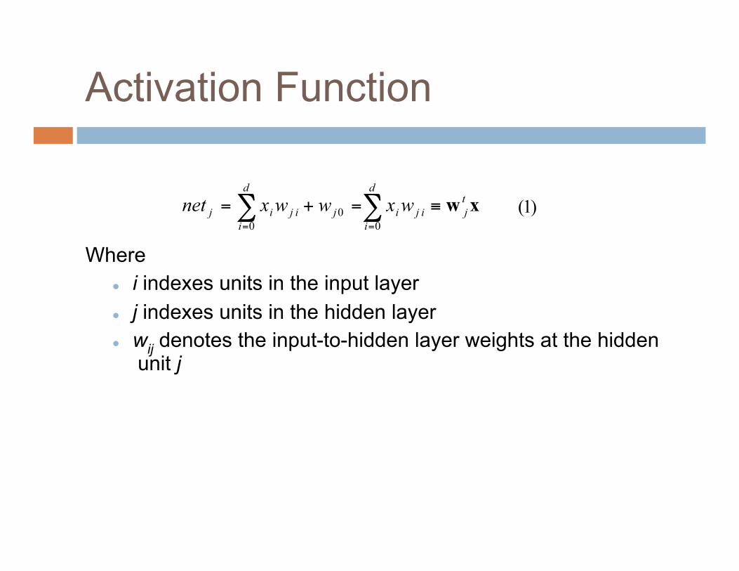
Activation Function

Where   i indexes units in the input layer   j indexes units in the hidden layer   wij denotes the input-to-hidden layer weights at the hidden

unit j

Activation Function

Each hidden unit emits an output that is a nonlinear function of its activation, f(net), that is:

One possible activation function is simply the sign function:

The activation function represents the nonlinearity of a unit. The activation function is sometimes referred to as a sigmoid function,

a squashing function, since its primary purpose is to limit the output of the neuron to some reasonable range like a range of -1 to +1, and thereby inject some degree of non-linearity into the network.

)2(‏

Activation Function

Because tanh is asymptotic when producing outputs of ±1, the network should be trained for an intermediate value such as ±.8.

LeCun suggests the hyperbolic tangent function as a good activation function. tanh is completely symmetric:

Also, the derivative of tanh is simply 1-tanh2, so if f(net) = tanh(net), then the derivative is simply 1-tanh2(net). When we discuss the update rule you will see why an activation

function with an easy-to-compute derivative is desirable.

Activation Function

Each output unit similarly computes its net activation based on the hidden unit signals as:

Where:   k indexes units in the output layer   nh denotes the number of hidden units

Equation 4 is basically the same as Equation 1. The only difference is are the indexes.

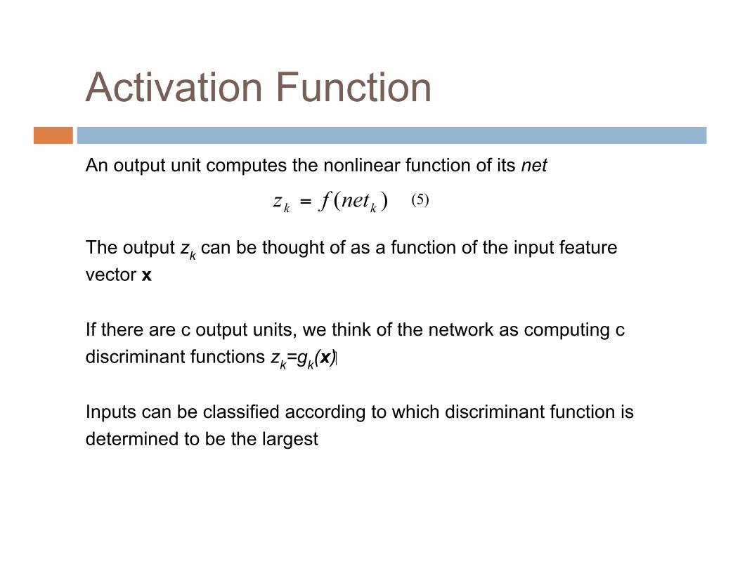
Activation Function

An output unit computes the nonlinear function of its net

The output zk can be thought of as a function of the input feature vector x

If there are c output units, we think of the network as computing c discriminant functions zk=gk(x)‏

Inputs can be classified according to which discriminant function is determined to be the largest

General Feedforward Operation

Given a sufficient number of hidden units of a general type any function can be represented by the hidden layer

This also applies to:   More inputs   Other nonlinearities   Any number of output units

Equations 1, 2, 4, and 5 can be combined to express the discriminant function gk(x):

Expressive Power

Any continuous function from input to output can be implemented in a three layer network given   A sufficient number of of hidden units nH   Proper nonlinearities   Weights

Kolmogorov proved that any continuous function g(x) defined on the hypercube In (I = [0,1] and n ≥ 2) can be represented in the form

Expressive Power

Equation 8 can be expressed in neural network terminology as follows:   Each of the 2n + 1 hidden units takes as input a sum of d

nonlinear functions, one for each input feature xi   Each hidden unit emits a nonlinear function of its total input   The output unit emits the sum of the contributions of the hidden

units

Expressive Power

Figure 6.2 represents a 2-4-1 network, with a bias.

Each hidden output unit has a sigmoidal activation function f(·)

The hidden output units are paired in opposition and thus produce a “bump” at the output unit.

Given a sufficiently large number of hidden units, any continuous function from input to output can be approximated arbitrarily well by such a network.

Expressive Power

Backpropagation Learning Rule

“Backpropagation of Errors” – during training an error must be propagated from the output layer back to the hidden layer in order learn input-to-hidden weights

Credit Assignment Problem – there is no explicit teacher to tell us what the hidden unit’s output should be

Backpropagation is used for the supervised learning of networks.

Modes of Operation

Networks have 2 primary modes of operation:

  Feed-forward Operation – present a pattern to the input units and pass signals through the network to yield outputs from the output units (ex. XOR network)

  Supervised Learning – present an input pattern and change the network parameters to bring the actual outputs closer to desired target values

3-Layer Neural Network Notation d – dimensions of input pattern x xi – signal emitted by input unit i

(ex. pixel value for an input image)

nH – number of hidden units f() – nonlinear activation function wji – weight of connection between input

unit i and hidden unit j netj – inner product of input signals with

weights wij at the hidden unit j yj – signal emitted by hidden unit j,

yj = f(netj) wkj – weight of connection between input

hidden unit j and output unit k

netk – inner product of hidden signals with weights wkj at the output unit k

zk – signal emitted by output unit k (one for each classifier), zk = f(netk)

t – target vector that output signals z are compared with to find differences between actual and desired values

c – number of classes (size of t and z)

Training Error

Using t and z we can determine the training error of a given pattern using the following criterion function:

(9)

Which gives us half the sum of the squared difference between the desired output tk and the actual output zk over all outputs. This is based on the vector of current weights in the network, w.

(44)

Looks very similar to the the Minimum Squared Error criterion function:

Y– n-by- matrix of x space feature points to y space feature points in dimensions

a – dimensional weight vector b – margin vector

Update Rule: Hidden Units to Output Units

Weights are initialized with random values and changed in a direction that will reduce the error:

(10)

η – learning rate that controls the relative size of the change in weights

(12)

The weight vector is updated per iteration m, as follows:

(11)

Let’s evaluate Δw for a 3-layer network for the output weights wkj:

(13)

yj

(14)

(4)

Sensitivity of unit k describes how the overall error changes with respect to the unit’s net activation:

Looks a lot like the Least Mean Squared Rule when f’(netk)=1:

(15)

(9) (5)

After plugging it all in we have the weight update / learning rule:

(17)

Iterative form:

(61)

If we get the correct outputs, tk = zk, then Δwkj = 0 as desired

Update Rule: Hidden Units to Output Units

The update rule for a connection weight between hidden unit j and output unit k :

Working backwards from outputs to inputs, we need to find the update rule for a connection weight between input unit i and hidden unit j:

(21)

Intuitive

reasoning

Update Rule: Input Units to Hidden Units

Backpropagation Analysis What if we set the all the initial weights, wkj, to 0 in the update rule?

(21)

Clearly, Δwji = 0 and the weights would never change. It would be bad of all network weights were ever equal to 0. This is why we start the network with random weights.

The update rules discussed only apply to a 3-layer network where all of the connections were between a layer and it’s preceeding layer.

The concepts can be generalized to apply to a network with n hidden layers, to include bias units, to handle a different learning rate for each unit, etc.

It’s more difficult to apply these concepts to recurrent networks where there are connections from higher layers back to lower layers/

Training Protocols Training consists of presenting to the network the collection of patters whose category we know, collectively known as the training set. Then we go about finding the output of the network and adjusting the weights to make the next output more like the desired target values.

The three most useful training protocols are: •  Stochastic •  On-Line •  Batch

In the stochastic and batch training methods, we will usually make several passes through the training data. For on-line training, we will use each pattern once and only once.

We use the term epoch to describe the overall number of training set passes. The number of epochs is an indication of the relative amount of learning.

Stochastic Training In stochastic training patterns are chosen at random from the training set and network weights are updated for each pattern presentation.

Stochastic Back propagation Algorithm

1.  begin initialize , w, criterion , , m 0

2.  do m m + 1

3.  randomly chosen pattern

4.  + ; +

5.  until <

6.  return w

7.  end

On-Line Training In on-line training, each pattern is presented once and only once. There is no use of memory for storing the patterns.

Useful for live training with human testers. On-line Back propagation Algorithm

1.  begin initialize , w, criterion , , m 0

2.  do m m+1

3.  select a new, unique pattern to be used

4.  + ; +

5.  until <

6.  return w

7.  end

Batch Training In batch training, the entire training set is presented first and their corresponding weight updates are summed; from there the actual weights in the network are updated. This process is iterated until the stopping criteria is met.

The total training error over n individual patterns can be written as:

Batch Back propagation Algorithm

1.  begin initialize , w, criterion , , m 0

2.  do r m+1 (increment epoch)

3.  m 0;

4.  do m m+1

5.  = select pattern

6. 

7.  until m=n

8. 

9.  until <

10.  return w

11.  end

Learning Curves training set – network hones weights using update rule test set – estimate generalization error due to weight training; performance of fielded

network.

validation set – represent novel patterns not yet classified training usually stopped at first minimum of validation set

low expressive power (few network weights) + high Bayes error = high asymptotic training error

Convolutional kernel application example:

Convolutional Neural Network

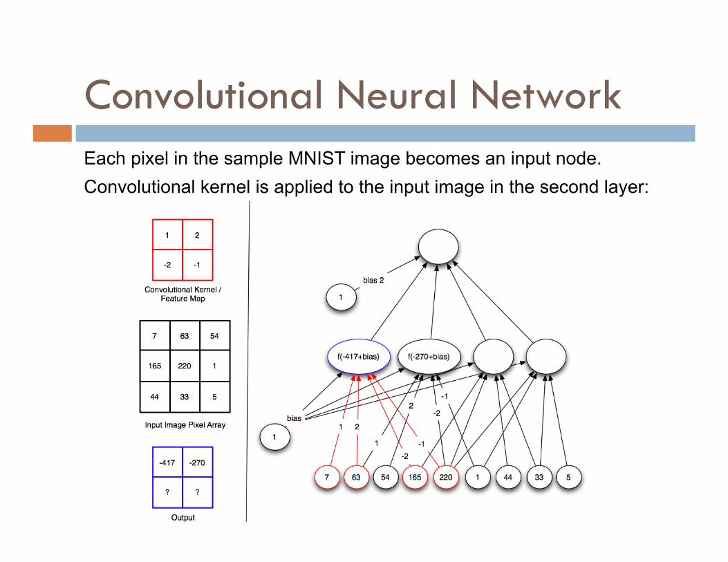
Each pixel in the sample MNIST image becomes an input node. Convolutional kernel is applied to the input image in the second layer:

Convolutional Neural Network

Simard recommends a convolutional neural network consisting of 5 layers.

Input layer consists of one neuron per pixel in a 29x29 padded MNIST sample image

First layer applies 6 feature maps to the input layer. Each map is a randomly distributed 5x5 kernel. Second layer applies 50 feature maps to all 6 previous maps. Each map is a randomly distributed 5x5 kernel.

First and second layers referred to as trainable feature extractor.

Third and fourth layers are fully connected and compose a universal classifier with 100 hidden units.

Third and fourth layers referred to as a trainable feature classifier.

Convolutional Neural Network Applied to Handwritten Digit Recognition

http://www.codeproject.com/KB/library/ NeuralNetRecognition/IllustrationNeuralNet.gif

Structural Adaptability One of the biggest issues with neural networks is the selection of a suitable structure for the network. This is especially true in unknown environments.

Lee Tsu-Chang developed a method for altering the structure of the neural network during the learning process.

If, during training, the error has stabilized but is larger than our target error, we will generate a new hidden layer neuron.

A neuron can be annihilated when it is no longer a functioning element of the network. This occurs if the neuron is a redundant element, has a constant output, or is entirely dependent on another neuron.

These criteria can be checked by monitoring the input weight vectors of neurons in the same layer. If two of them are linear dependent, then the represent the same hyper plane in the data space spanned by their receptive field and are totally dependent on each other. If the output is a constant value, then the output entropy is approximately zero.

This methodology is incredibly useful for finding the optimal design for a neural network without requiring extensive domain knowledge.

Structural Adaptability

In the graph to the right, the letters A, B, and C represent the times when structural adaptability caused a hidden layer neuron to be removed. Note that these occurred at performance plateaus and did in fact improve the error rate.

The error rate was calculated for an OCR network over each upper-case English letter.

References Duda, R., Hart, P., Stork, D. Pattern Classification, 2nd ed. John Wiley & Sons, 2001.

Y. LeCun, L. Bottou, G.B. Orr, and K.-R. Muller. Efficient Backprop. Neural Networks: Tricks of the Trade, Springer Lecture Notes in Computer Sciences, No. 1524, pp. 5-50, 1998.

P. Simard, D. Steinkraus, and J. Platt. Best Practice for Convolutional Neural Networks Applied to Visual Document Analysis. International Conference on Document Analysis and Recognition, ICDAR 2003, IEEE Computer Society, Vol. 2, pp. 958-962, 2003.

L. Tsu-Chang, Structure Level Adaptation for Artificial Neural Networks, Kluwer Academic Publishers, Boston, 1991.

Ramirez, J.M.; Gomez-Gil, P.; Baez-Lopez, D., "On structural adaptability of neural networks in character recognition," Signal Processing, 1996., 3rd International Conference on , vol.2, no., pp.1481-1483 vol.2, 14-18 Oct 1996