Multilayer Neural Networks

1

Introduction

• Goal: Classify objects by learning nonlinearity

– There are many problems for which lineardiscriminants are insufficient for minimum error

– In previous methods, the central difficulty was thechoice of the appropriate nonlinear functions

– A “brute” approach might be to select a complete basisset such as all polynomials; such a classifier wouldrequire too many parameters to be determined from alimited number of training samples

2

– There is no automatic method for determining thenonlinearities when no information is provided tothe classifier

– In using the multilayer Neural Networks, the formof the nonlinearity is learned from the training data

3

Feedforward Operation and Classification

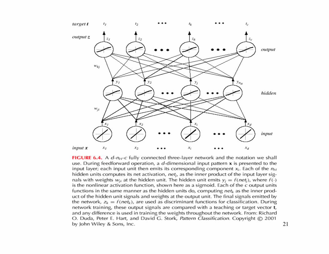
• A three-layer neural network consists of aninput layer, a hidden layer and an output layerinterconnected by modifiable weightsrepresented by links between layers

4

5

6

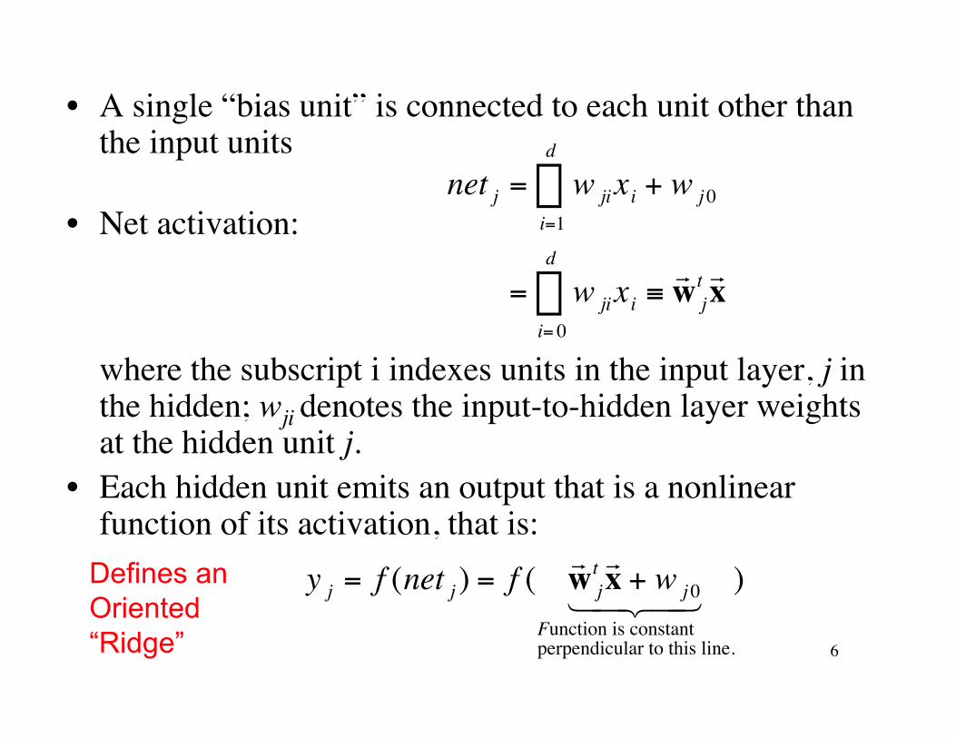
• A single “bias unit” is connected to each unit other thanthe input units

• Net activation:

where the subscript i indexes units in the input layer, j inthe hidden; wji denotes the input-to-hidden layer weightsat the hidden unit j.

• Each hidden unit emits an output that is a nonlinearfunction of its activation, that is:

†

net j = w jixi + w j 0i=1

d

Â

= w jixi ≡r w jt

r x i= 0

d

Â

†

y j = f (net j ) = f ( r w jtr x + w j 0

Function is constantperpendicular to this line.

1 2 4 3 4 )Defines an

Oriented “Ridge”

7

8

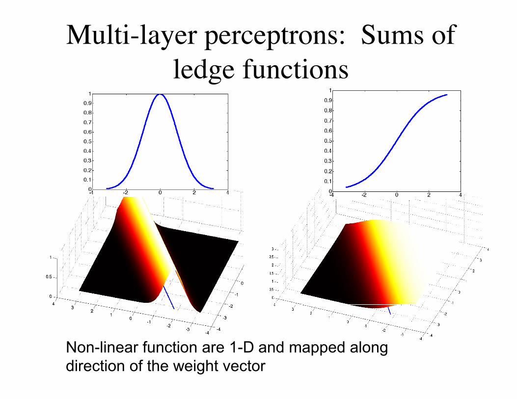
Multi-layer perceptrons: Sums ofledge functions

Non-linear function are 1-D and mapped alongdirection of the weight vector

9

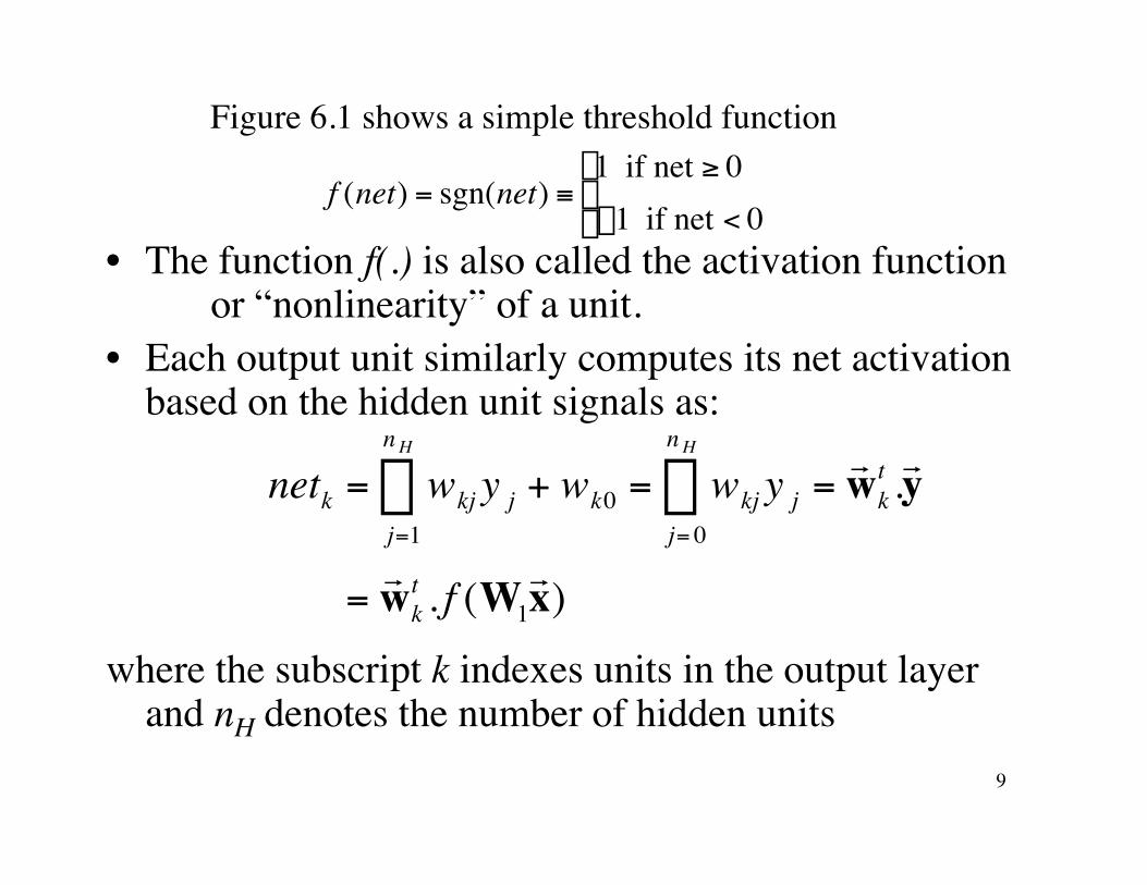
Figure 6.1 shows a simple threshold function

• The function f(.) is also called the activation functionor “nonlinearity” of a unit.

• Each output unit similarly computes its net activationbased on the hidden unit signals as:

where the subscript k indexes units in the output layerand nH denotes the number of hidden units

†

f (net) = sgn(net) ≡1 if net ≥ 0-1 if net < 0

Ï Ì Ó

†

netk = wkj y j + wk0 = wkj y j =r w kt .r y

j= 0

n H

Âj=1

n H

Â

=r w kt . f (W1

r x )

10

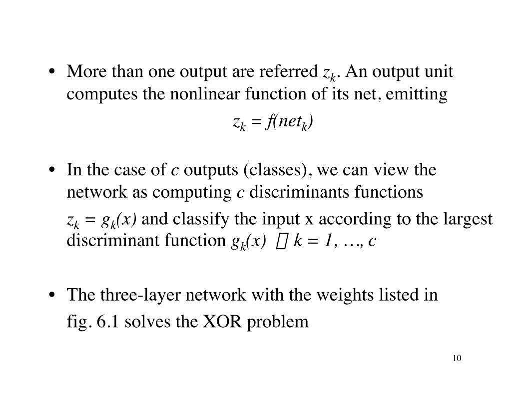
• More than one output are referred zk. An output unitcomputes the nonlinear function of its net, emitting

zk = f(netk)

• In the case of c outputs (classes), we can view thenetwork as computing c discriminants functionszk = gk(x) and classify the input x according to the largestdiscriminant function gk(x) " k = 1, …, c

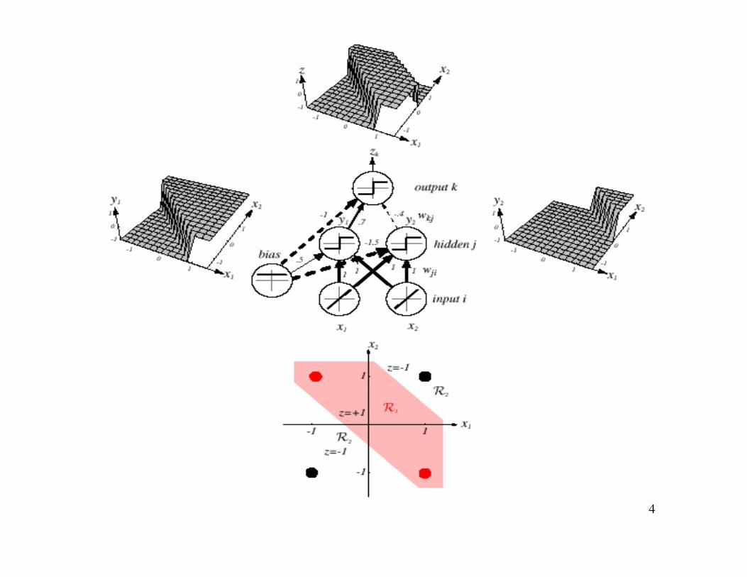
• The three-layer network with the weights listed infig. 6.1 solves the XOR problem

11

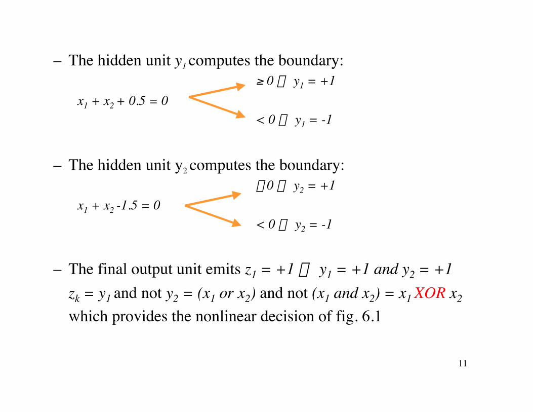
– The hidden unit y1 computes the boundary: ≥ 0 fi y1 = +1

x1 + x2 + 0.5 = 0 < 0 fi y1 = -1

– The hidden unit y2 computes the boundary: £ 0 fi y2 = +1

x1 + x2 -1.5 = 0 < 0 fi y2 = -1

– The final output unit emits z1 = +1 ¤ y1 = +1 and y2 = +1zk = y1 and not y2 = (x1 or x2) and not (x1 and x2) = x1 XOR x2

which provides the nonlinear decision of fig. 6.1

12

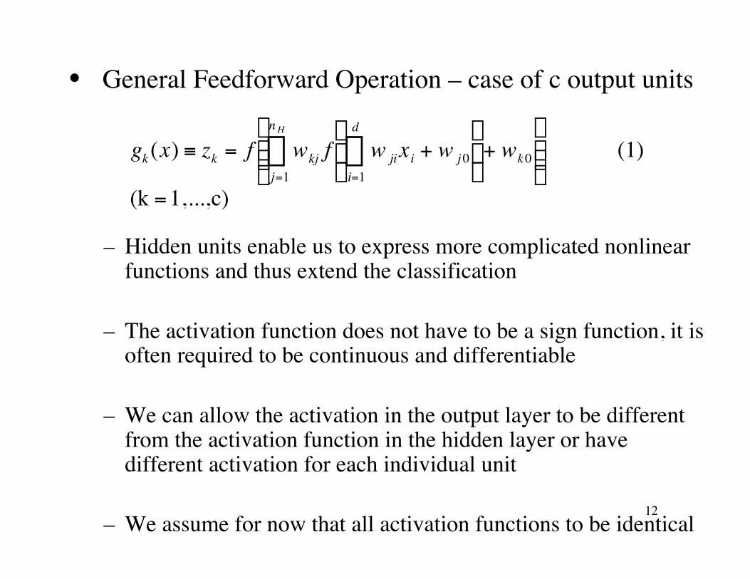
• General Feedforward Operation – case of c output units

– Hidden units enable us to express more complicated nonlinearfunctions and thus extend the classification

– The activation function does not have to be a sign function, it isoften required to be continuous and differentiable

– We can allow the activation in the output layer to be differentfrom the activation function in the hidden layer or havedifferent activation for each individual unit

– We assume for now that all activation functions to be identical

†

gk(x) ≡ zk = f wkj f w jixi + w j 0i=1

d

ÂÊ

Ë Á

ˆ

¯ ˜ + wk 0

j=1

n H

ÂÊ

Ë Á Á

ˆ

¯ ˜ ˜ (1)

(k =1,...,c)

13

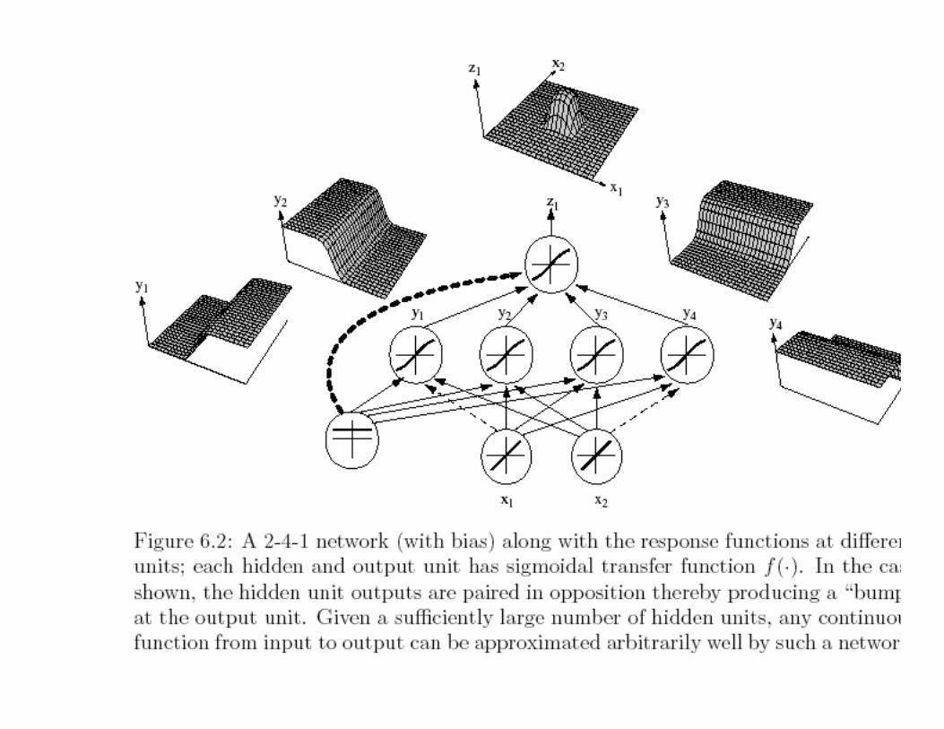
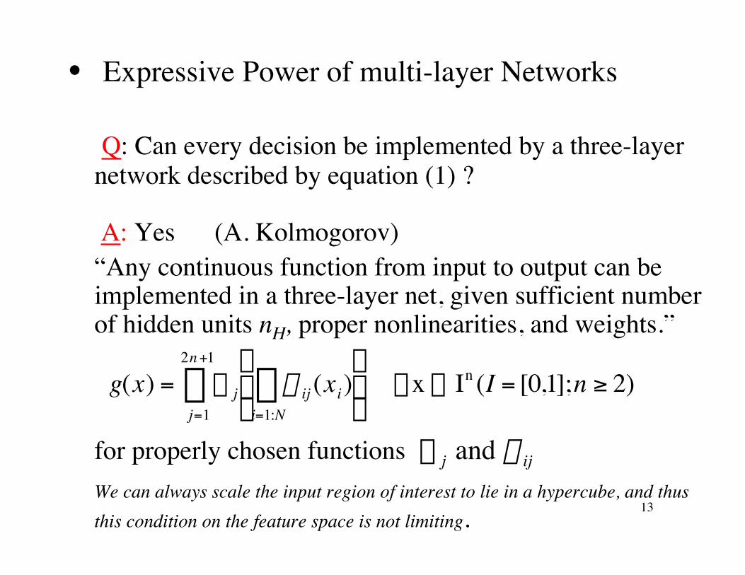
• Expressive Power of multi-layer Networks

Q: Can every decision be implemented by a three-layernetwork described by equation (1) ?

A: Yes (A. Kolmogorov)“Any continuous function from input to output can beimplemented in a three-layer net, given sufficient numberof hidden units nH, proper nonlinearities, and weights.”

for properly chosen functionsWe can always scale the input region of interest to lie in a hypercube, and thusthis condition on the feature space is not limiting.†

g(x) = X j y ij (xi)i=1:NÂ

Ê

Ë Á

ˆ

¯ ˜

j=1

2n +1

 "x Œ In (I = [0,1];n ≥ 2)

†

X j and yij

14

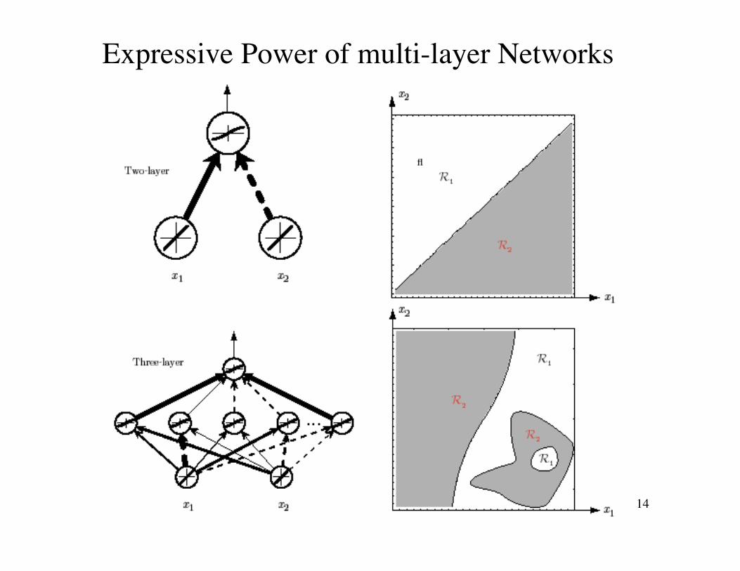
Expressive Power of multi-layer Networks

15

• Each of the 2n+1 hidden units takes as input asum of N nonlinear functions, one for each inputfeature xi

Unfortunately: Kolmogorov’s theorem tells usvery little about how to find the nonlinearfunctions based on data; this is the centralproblem in network-based pattern recognition.

Moreover, any specific network structure specializesthe above formulation, and hence most networksmust be viewed as approximating the targetfunction

†

X j

16

17

Backpropagation Algorithm

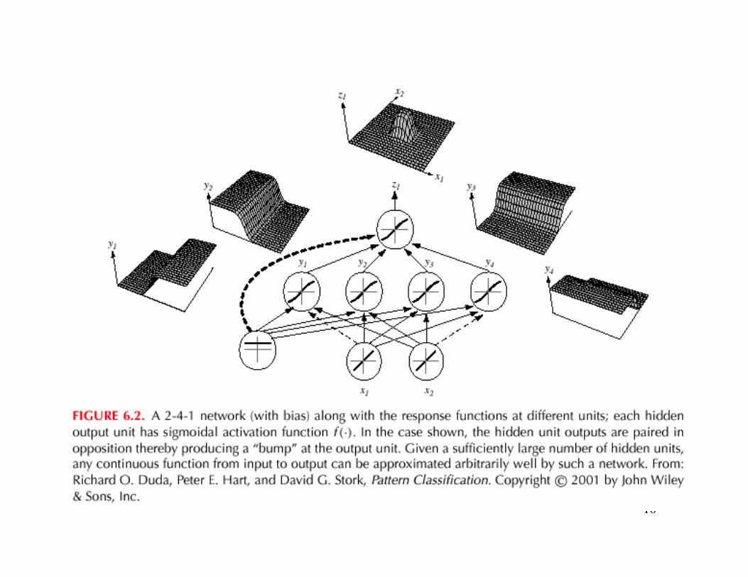
• Any function from input to output can beapproximated as a three-layer neuralnetwork

• How do we learn the approximation?

18

19

• Our goal now is to set the interconnexion weightsbased on the training patterns and the desired outputs

• In a three-layer network, it is a straightforward matterto understand how the output, and thus the error,depend on the hidden-to-output layer weights

• The power of backpropagation is that it enables us tocompute an effective error for each hidden unit, andthus derive a learning rule for the input-to-hiddenweights, this is known as:

The credit assignment problem

20

• Network have two modes of operation:

– FeedforwardThe feedforward operations consists of presenting apattern to the input units and passing (or feeding) thesignals through the network in order to get outputs units(no cycles!)

– LearningThe supervised learning consists of presenting an inputpattern and modifying the network parameters (weights) toreduce distances between the computed output and thedesired output

21

22

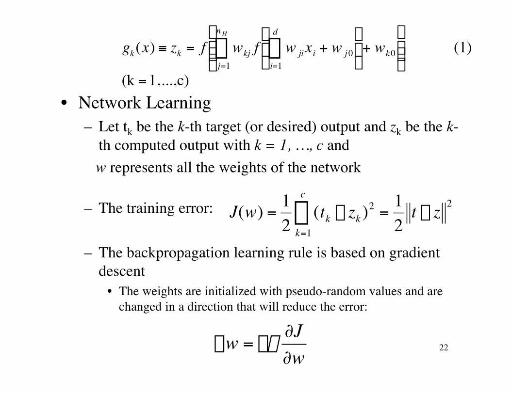
• Network Learning– Let tk be the k-th target (or desired) output and zk be the k-

th computed output with k = 1, …, c and w represents all the weights of the network

– The training error:

– The backpropagation learning rule is based on gradientdescent

• The weights are initialized with pseudo-random values and arechanged in a direction that will reduce the error:†

J(w) =12

(tk - zk )2 =12

t - z 2

k=1

c

Â

†

Dw = -h∂J∂w

†

gk(x) ≡ zk = f wkj f w jixi + w j 0i=1

d

ÂÊ

Ë Á

ˆ

¯ ˜ + wk 0

j=1

n H

ÂÊ

Ë Á Á

ˆ

¯ ˜ ˜ (1)

(k =1,...,c)

23

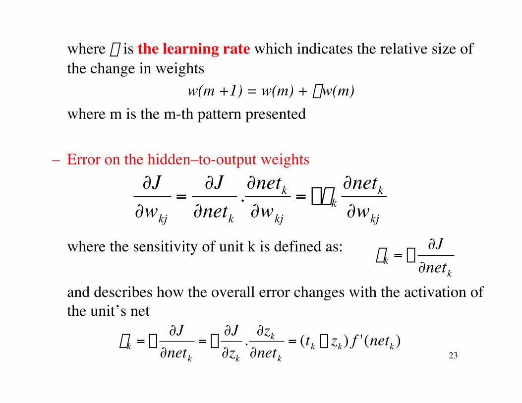
where h is the learning rate which indicates the relative size ofthe change in weights

w(m +1) = w(m) + Dw(m)where m is the m-th pattern presented

– Error on the hidden–to-output weights

where the sensitivity of unit k is defined as:

and describes how the overall error changes with the activation ofthe unit’s net†

∂J∂wkj

=∂J

∂netk

.∂netk

∂wkj

= -dk∂netk

∂wkj

†

dk = -∂J

∂netk

†

dk = -∂J

∂netk

= -∂J∂zk

. ∂zk

∂netk

= (tk - zk) f '(netk )

24

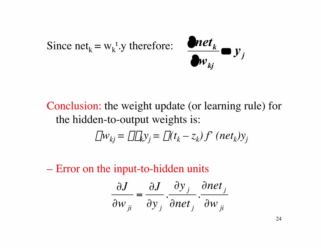
Since netk = wkt.y therefore:

Conclusion: the weight update (or learning rule) forthe hidden-to-output weights is:

Dwkj = hdkyj = h(tk – zk) f’ (netk)yj

– Error on the input-to-hidden units

jkj

k yw

net=

∂

∂

†

∂J∂w ji

=∂J∂y j

.∂y j

∂net j

.∂net j

∂w ji

25

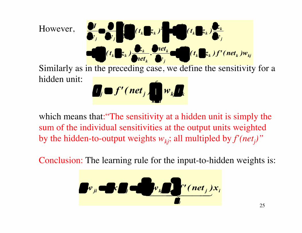
However,

Similarly as in the preceding case, we define the sensitivity for ahidden unit:

which means that:“The sensitivity at a hidden unit is simply thesum of the individual sensitivities at the output units weightedby the hidden-to-output weights wkj; all multipled by f’(netj)”

Conclusion: The learning rule for the input-to-hidden weights is:

 Â

ÂÂ

= =

==

--=∂

∂

∂

∂--=

∂

∂--=˙

˚

˘ÍÎ

È-

∂

∂=

∂

∂

c

1k

c

1kkjkkk

j

k

k

kkk

c

1k j

kkk

2k

c

1kk

jj

w)net('f)zt(y

net.

net

z)zt(

y

z)zt()zt(

21

yyJ

Â=

≡c

1kkkjjj w)net('f dd

[ ] ijkkjjiji x)net('f wxw

j

444 3444 21d

dShdhD ==

26

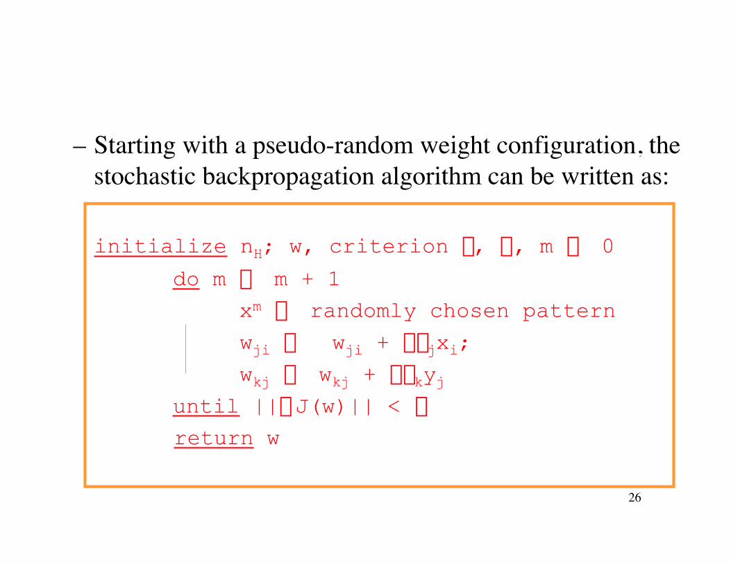
– Starting with a pseudo-random weight configuration, thestochastic backpropagation algorithm can be written as:

initialize nH; w, criterion q, h, m ¨ 0

do m ¨ m + 1

xm ¨ randomly chosen pattern

wji ¨ wji + hdjxi;

wkj ¨ wkj + hdkyjuntil ||—J(w)|| < q

return w

28

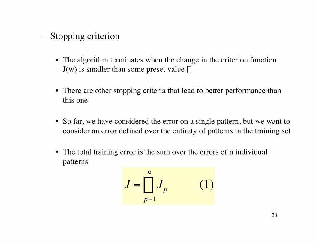
– Stopping criterion

• The algorithm terminates when the change in the criterion functionJ(w) is smaller than some preset value q

• There are other stopping criteria that lead to better performance thanthis one

• So far, we have considered the error on a single pattern, but we want toconsider an error defined over the entirety of patterns in the training set

• The total training error is the sum over the errors of n individualpatterns

†

J = Jpp=1

n

 (1)

29

– Stopping criterion (cont.)

• A weight update may reduce the error on the singlepattern being presented but can increase the error on thefull training set

• However, given a large number of such individualupdates, the total error of equation (1) decreases

30

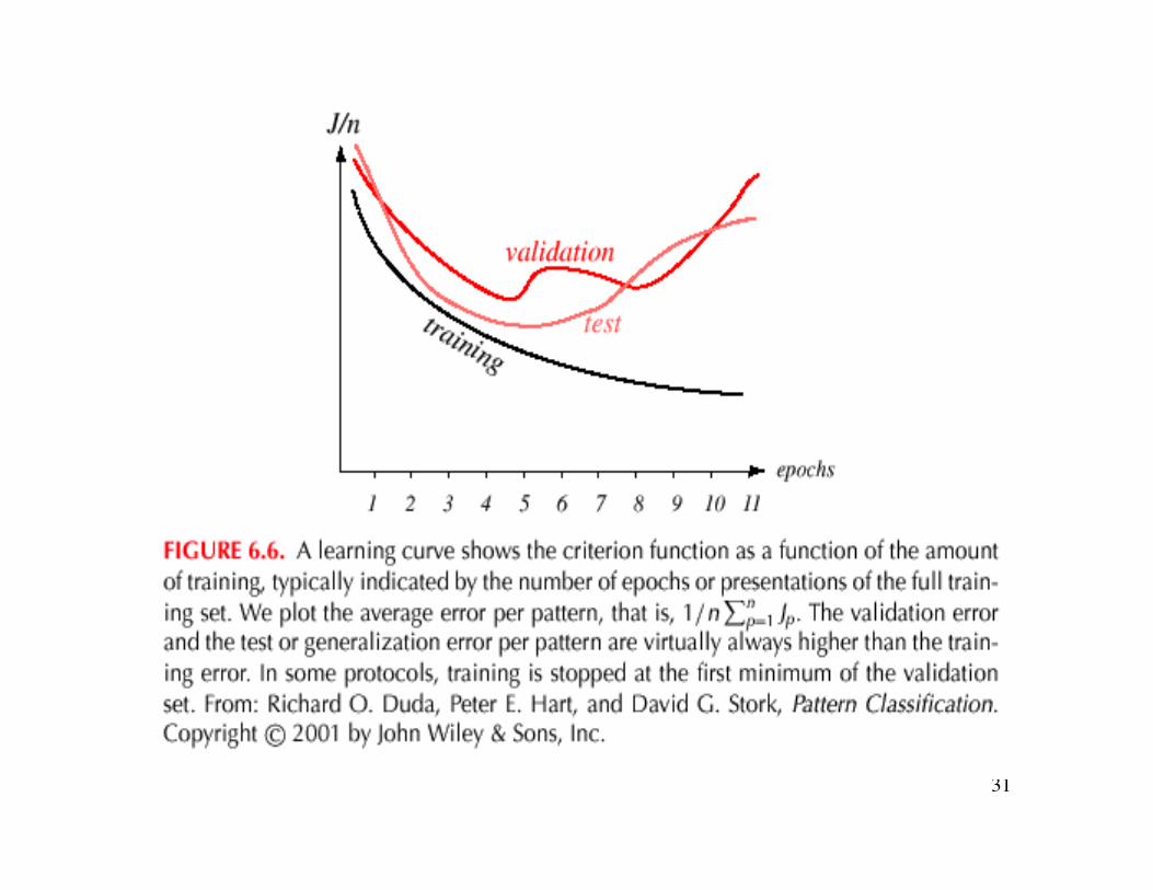
• Learning Curves– Before training starts, the error on the training set is high;

through the learning process, the error becomes smaller

– The error per pattern depends on the amount of training dataand the expressive power (such as the number of weights) inthe network

– The average error on an independent test set is always higherthan on the training set, and it can decrease as well asincrease

– A validation set is used in order to decide when to stoptraining ; we do not want to overfit the network and decreasethe power of the classifier generalization“we stop training at a minimum of the error on the validationset”

31