multilayer perceptron and neural networks - wseas · multilayer perceptron and neural networks...

Multilayer Perceptron and Neural Networks

MARIUS-CONSTANTIN POPESCU1 VALENTINA E. BALAS2 LILIANA PERESCU-POPESCU3 NIKOS MASTORAKIS4

Faculty of Electromechanical and Environmental Engineering, University of Craiova1 Faculty of Engineering, “Aurel Vlaicu” University of Arad2

“Elena Cuza” College of Craiova3 ROMANIA,

Technical University of Sofia4 BULGARIA.

[email protected] [email protected] [email protected]

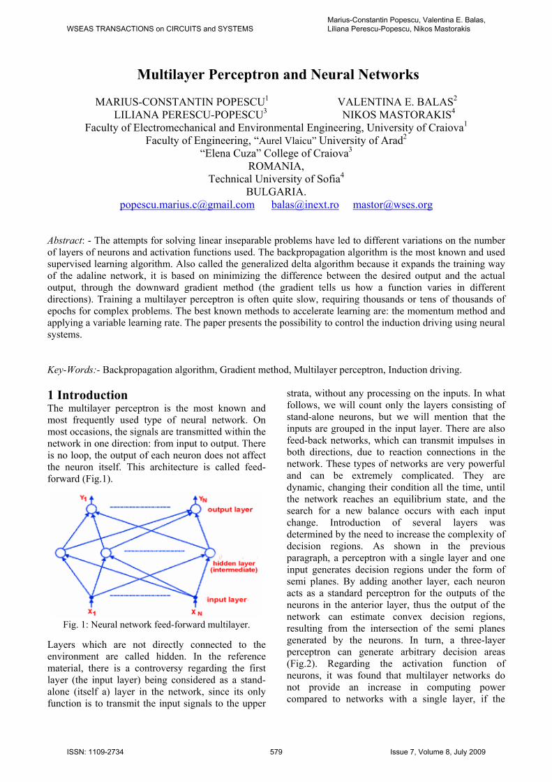
Abstract: - The attempts for solving linear inseparable problems have led to different variations on the number of layers of neurons and activation functions used. The backpropagation algorithm is the most known and used supervised learning algorithm. Also called the generalized delta algorithm because it expands the training way of the adaline network, it is based on minimizing the difference between the desired output and the actual output, through the downward gradient method (the gradient tells us how a function varies in different directions). Training a multilayer perceptron is often quite slow, requiring thousands or tens of thousands of epochs for complex problems. The best known methods to accelerate learning are: the momentum method and applying a variable learning rate. The paper presents the possibility to control the induction driving using neural systems. Key-Words:- Backpropagation algorithm, Gradient method, Multilayer perceptron, Induction driving. 1 Introduction The multilayer perceptron is the most known and most frequently used type of neural network. On most occasions, the signals are transmitted within the network in one direction: from input to output. There is no loop, the output of each neuron does not affect the neuron itself. This architecture is called feed-forward (Fig.1).

Fig. 1: Neural network feed-forward multilayer.

Layers which are not directly connected to the environment are called hidden. In the reference material, there is a controversy regarding the first layer (the input layer) being considered as a stand-alone (itself a) layer in the network, since its only function is to transmit the input signals to the upper

strata, without any processing on the inputs. In what follows, we will count only the layers consisting of stand-alone neurons, but we will mention that the inputs are grouped in the input layer. There are also feed-back networks, which can transmit impulses in both directions, due to reaction connections in the network. These types of networks are very powerful and can be extremely complicated. They are dynamic, changing their condition all the time, until the network reaches an equilibrium state, and the search for a new balance occurs with each input change. Introduction of several layers was determined by the need to increase the complexity of decision regions. As shown in the previous paragraph, a perceptron with a single layer and one input generates decision regions under the form of semi planes. By adding another layer, each neuron acts as a standard perceptron for the outputs of the neurons in the anterior layer, thus the output of the network can estimate convex decision regions, resulting from the intersection of the semi planes generated by the neurons. In turn, a three-layer perceptron can generate arbitrary decision areas (Fig.2). Regarding the activation function of neurons, it was found that multilayer networks do not provide an increase in computing power compared to networks with a single layer, if the

WSEAS TRANSACTIONS on CIRCUITS and SYSTEMSMarius-Constantin Popescu, Valentina E. Balas, Liliana Perescu-Popescu, Nikos Mastorakis

ISSN: 1109-2734 579 Issue 7, Volume 8, July 2009

mailto:[email protected]



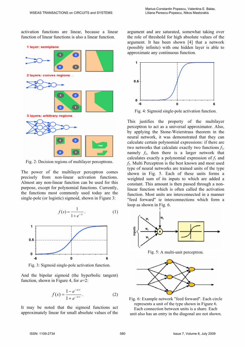
activation functions are linear, because a linear function of linear functions is also a linear function.

Fig. 2: Decision regions of multilayer perceptrons.

The power of the multilayer perceptron comes precisely from non-linear activation functions. Almost any non-linear function can be used for this purpose, except for polynomial functions. Currently, the functions most commonly used today are the single-pole (or logistic) sigmoid, shown in Figure 3:

sesf −+=

11)( . (1)

Fig. 3: Sigmoid single-pole activation function.

And the bipolar sigmoid (the hyperbolic tangent) function, shown in Figure 4, for a=2:

sa

sa

eesf ⋅−

⋅−

+−

=11)( . (2)

It may be noted that the sigmoid functions act approximately linear for small absolute values of the

argument and are saturated, somewhat taking over the role of threshold for high absolute values of the argument. It has been shown [4] that a network (possibly infinite) with one hidden layer is able to approximate any continuous function.

Fig. 4: Sigmoid single-pole activation function.

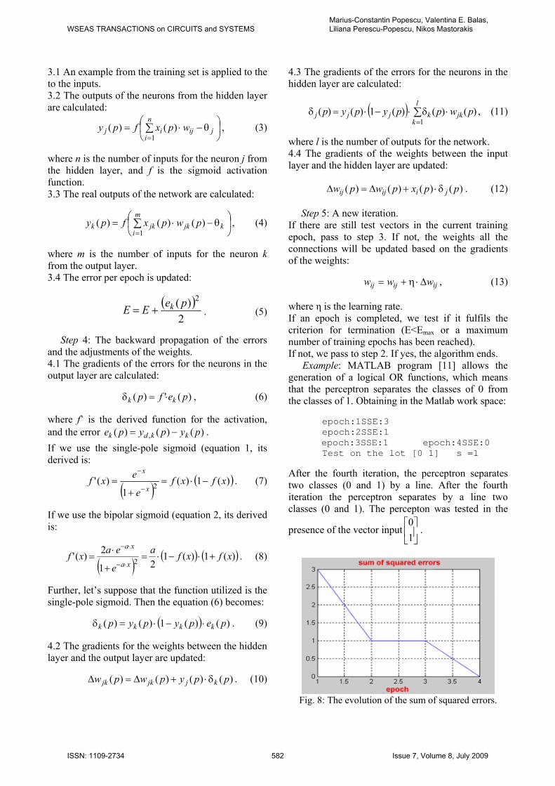
This justifies the property of the multilayer perceptron to act as a universal approximator. Also, by applying the Stone-Weierstrass theorem in the neural network, it was demonstrated that they can calculate certain polynomial expressions: if there are two networks that calculate exactly two functions f1, namely f2, then there is a larger network that calculates exactly a polynomial expression of f1 and f2. Multi Perceptron is the best known and most used type of neural networks are trained units of the type shown in Fig. 5. Each of these units forms a weighted sum of its inputs to which are added a constant. This amount is then passed through a non-linear function which is often called the activation function. Most units are interconnected in a manner "feed forward" ie interconnections which form a loop as shown in Fig. 6.

Fig. 5: A multi-unit perceptron.

Fig. 6: Example network "feed forward". Each circle

represents a unit of the type shown in Figure 6. Each connection between units is a share. Each

unit also has an entry in the diagonal are not shown.



For some types of applications recurrent networks (ie not "feed forward"), in which some interconnections forming loop, are also used. I have seen in Figure 6 an example of feed forward network. As mentioned interconnections units of this type of network does a not form loop, so the network is called feed forward. Networks in which there is one or more loops of interconnections as represented in Figure 7.a shall appoint recurring between the units has a share. Each unit also has an entry in the diagonal are not shown.

a)

b)

c)

d)

Fig. 7: Common types of networks: a) a recurrent network; b) a stratified network; c) a network with links between units of input and output; d) a feed

forward network fully connected.

In feed forward networks, units are usually arranged in levels (layers) as in Figure 7.b but other topologies can be used. Figure 7.c shows a type of network that is useful in some applications in which direct links between units of input and output are used. Figure 7.d shows a network with 3 units which is fully connected i.e. that all interconnections are allowed to feed restriction forward.

2 The backpropagation algorithm

Learning networks is typically achieved through a supervised manner. It can be assumed to be available a learning environment that contains both the learning models and models of desired output corresponding to input (this is known as "target models"). As we will see, learning is typically based on the minimization of measurement errors between network outputs and desired outputs. This implies a back propagation through a network similar to that which is learned. For this reason algorithm learning is called back-propagation. The method was first proposed by [2], but at that time it was virtually ignored, because it supposed volume calculations too large for that time. It was then rediscovered by [20], but only in the mid-'80s was launched by Williams [18] as a generally accepted tool for training of the multilayer perceptron. The idea is to find the minimum error function e(w) in relation to the connections weights. The algorithm for a multilayer perceptron with a hidden layer is the following [8]: Step 1: Initializing. All network weights and thresholds are initialized with random values, distributed evenly in a small range, for example

⎟⎟⎠

⎞⎜⎜⎝

⎛ −

ii F.,

F. 4242 , where Fi is the total number of inputs

of the neuron i [6]. If these values are 0, the gradients which will be calculated during the trial will be also 0 (if there is no direct link between input and output) and the network will not learn. More training attempts are indicated, with different initial weights, to find the best value for the cost function (minimum error). Conversely, if initial values are large, they tend to saturate these units. In this case, derived sigmoid function is very small. It acts as a multiplier factor during the learning process and thus the saturated units will be nearly blocked, which makes learning very slow. Step 2: A new era of training. An era means presenting all the examples in the training set. In most cases, training the network involves more training epochs. To maintain mathematical rigor, the weights will be adjusted only after all the test vectors will be applied to the network. Therefore, the gradients of the weights must be memorized and adjusted after each model in the training set, and the end of an epoch of training, the weights will be changed only one time (there is an „on-line” variant, more simple, in which the weights are updated directly, in this case, the order in which the vectors of the network are presented might matter. All the gradients of the weights and the current error are initialized with 0 (Δwij = 0 and E = 0). Step 3: The forward propagation of the signal



3.1 An example from the training set is applied to the to the inputs. 3.2 The outputs of the neurons from the hidden layer are calculated:

⎟⎠

⎞⎜⎝

⎛ θ−⋅= ∑=

n

ijijij wpxfpy

1)()( , (3)

where n is the number of inputs for the neuron j from the hidden layer, and f is the sigmoid activation function. 3.3 The real outputs of the network are calculated:

⎟⎠

⎞⎜⎝

⎛ θ−⋅= ∑=

m

ikjkjkk pwpxfpy

1)()()( , (4)

where m is the number of inputs for the neuron k from the output layer. 3.4 The error per epoch is updated:

( )2

)( 2pe E E k+= . (5)

Step 4: The backward propagation of the errors and the adjustments of the weights. 4.1 The gradients of the errors for the neurons in the output layer are calculated:

)(')( pefp kk ⋅=δ , (6)

where f’ is the derived function for the activation, and the error )()()( , pypype kkdk −= . If we use the single-pole sigmoid (equation 1, its derived is:

( )( )(1)(

1)(' 2 xfxf

e

exfx

x−⋅=

+=

−

−) . (7)

If we use the bipolar sigmoid (equation 2, its derived is:

( )( ) ( )(1)(1

21

2)(' 2 xfxfa

e

eaxfxa

xa+⋅−⋅=

+

⋅=

⋅−

⋅−) . (8)

Further, let’s suppose that the function utilized is the single-pole sigmoid. Then the equation (6) becomes:

( ) )()(1)()( pepypyp kkkk ⋅−⋅=δ . (9)

4.2 The gradients for the weights between the hidden layer and the output layer are updated:

)()()()( ppypwpw kjjkjk δ⋅+Δ=Δ . (10)

4.3 The gradients of the errors for the neurons in the hidden layer are calculated:

( ) ∑=

⋅δ⋅−⋅=δl

kjkkjjj pwppypyp

1)()()(1)()( , (11)

where l is the number of outputs for the network. 4.4 The gradients of the weights between the input layer and the hidden layer are updated:

)()()()( ppxpwpw jiijij δ⋅+Δ=Δ . (12) Step 5: A new iteration. If there are still test vectors in the current training epoch, pass to step 3. If not, the weights all the connections will be updated based on the gradients of the weights:

ijijij www Δ⋅η+= , (13) where η is the learning rate. If an epoch is completed, we test if it fulfils the criterion for termination (E<Emax or a maximum number of training epochs has been reached). If not, we pass to step 2. If yes, the algorithm ends. Example: MATLAB program [11] allows the generation of a logical OR functions, which means that the perceptron separates the classes of 0 from the classes of 1. Obtaining in the Matlab work space: epoch:1SSE:3 epoch:2SSE:1

epoch:3SSE:1 epoch:4SSE:0 Test on the lot [0 1] s =1

After the fourth iteration, the perceptron separates two classes (0 and 1) by a line. After the fourth iteration the perceptron separates by a line two classes (0 and 1). The percepton was tested in the

presence of the vector input . ⎥⎦

⎤⎢⎣

⎡10

Fig. 8: The evolution of the sum of squared errors.



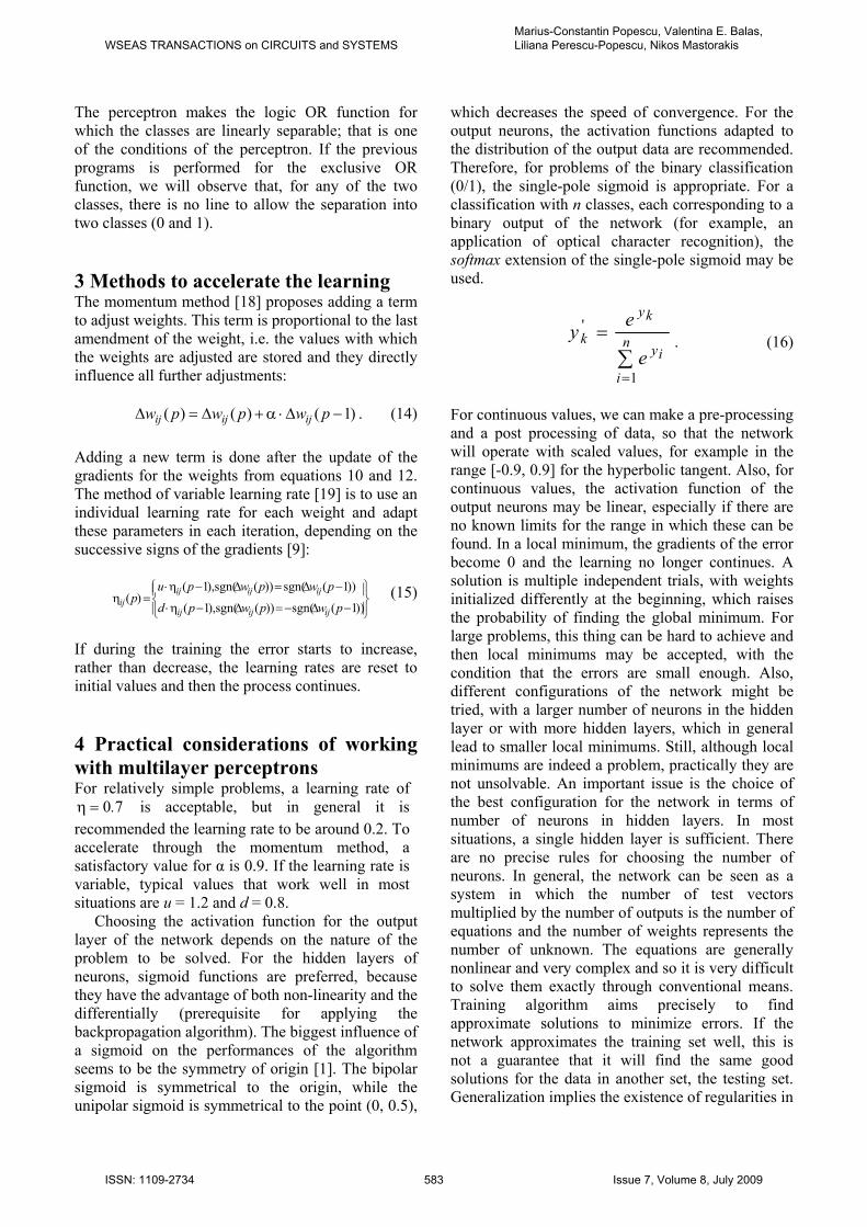
The perceptron makes the logic OR function for which the classes are linearly separable; that is one of the conditions of the perceptron. If the previous programs is performed for the exclusive OR function, we will observe that, for any of the two classes, there is no line to allow the separation into two classes (0 and 1). 3 Methods to accelerate the learning The momentum method [18] proposes adding a term to adjust weights. This term is proportional to the last amendment of the weight, i.e. the values with which the weights are adjusted are stored and they directly influence all further adjustments:

)1()()( −Δ⋅α+Δ=Δ pwpwpw ijijij . (14) Adding a new term is done after the update of the gradients for the weights from equations 10 and 12. The method of variable learning rate [19] is to use an individual learning rate for each weight and adapt these parameters in each iteration, depending on the successive signs of the gradients [9]:

⎪⎭

⎪⎬⎫

⎪⎩

⎪⎨⎧

−Δ−=Δ−η⋅

−Δ=Δ−η⋅=η

))1(sgn())(sgn(),1(

))1(sgn())(sgn(),1()(

pwpwpd

pwpwpup

ijijij

ijijijij

(15)

If during the training the error starts to increase, rather than decrease, the learning rates are reset to initial values and then the process continues. 4 Practical considerations of working with multilayer perceptrons For relatively simple problems, a learning rate of

is acceptable, but in general it is recommended the learning rate to be around 0.2. To accelerate through the momentum method, a satisfactory value for α is 0.9. If the learning rate is variable, typical values that work well in most situations are u = 1.2 and d = 0.8.

70.=η

Choosing the activation function for the output layer of the network depends on the nature of the problem to be solved. For the hidden layers of neurons, sigmoid functions are preferred, because they have the advantage of both non-linearity and the differentially (prerequisite for applying the backpropagation algorithm). The biggest influence of a sigmoid on the performances of the algorithm seems to be the symmetry of origin [1]. The bipolar sigmoid is symmetrical to the origin, while the unipolar sigmoid is symmetrical to the point (0, 0.5),

which decreases the speed of convergence. For the output neurons, the activation functions adapted to the distribution of the output data are recommended. Therefore, for problems of the binary classification (0/1), the single-pole sigmoid is appropriate. For a classification with n classes, each corresponding to a binary output of the network (for example, an application of optical character recognition), the softmax extension of the single-pole sigmoid may be used.

∑=

= n

i

iy

ky

ke

ey

1

'. (16)

For continuous values, we can make a pre-processing and a post processing of data, so that the network will operate with scaled values, for example in the range [-0.9, 0.9] for the hyperbolic tangent. Also, for continuous values, the activation function of the output neurons may be linear, especially if there are no known limits for the range in which these can be found. In a local minimum, the gradients of the error become 0 and the learning no longer continues. A solution is multiple independent trials, with weights initialized differently at the beginning, which raises the probability of finding the global minimum. For large problems, this thing can be hard to achieve and then local minimums may be accepted, with the condition that the errors are small enough. Also, different configurations of the network might be tried, with a larger number of neurons in the hidden layer or with more hidden layers, which in general lead to smaller local minimums. Still, although local minimums are indeed a problem, practically they are not unsolvable. An important issue is the choice of the best configuration for the network in terms of number of neurons in hidden layers. In most situations, a single hidden layer is sufficient. There are no precise rules for choosing the number of neurons. In general, the network can be seen as a system in which the number of test vectors multiplied by the number of outputs is the number of equations and the number of weights represents the number of unknown. The equations are generally nonlinear and very complex and so it is very difficult to solve them exactly through conventional means. Training algorithm aims precisely to find approximate solutions to minimize errors. If the network approximates the training set well, this is not a guarantee that it will find the same good solutions for the data in another set, the testing set. Generalization implies the existence of regularities in



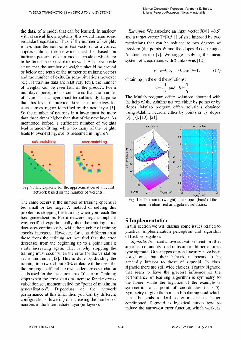
the data, of a model that can be learned. In analogy with classical linear systems, this would mean some redundant equations. Thus, if the number of weights is less than the number of test vectors, for a correct approximation, the network must be based on intrinsic patterns of data models, models which are to be found in the test data as well. A heuristic rule states that the number of weights should be around or below one tenth of the number of training vectors and the number of exits. In some situations however (e.g., if training data are relatively few), the number of weights can be even half of the product. For a multilayer perceptron is considered that the number of neurons in a layer must be sufficiently large so that this layer to provide three or more edges for each convex region identified by the next layer [5]. So the number of neurons in a layer must be more than three times higher than that of the next layer. As mentioned before, a sufficient number of weights lead to under-fitting, while too many of the weights leads to over-fitting, events presented in Figure 9.

Fig. 9: The capacity for the approximation of a neural

network based on the number of weights.

The same occurs if the number of training epochs is too small or too large. A method of solving this problem is stopping the training when you reach the best generalization. For a network large enough, it was verified experimentally that the training error decreases continuously, while the number of training epochs increases. However, for data different than those from the training set, we find that the error decreases from the beginning up to a point until it starts increasing again. That is why stopping the training must occur when the error for the validation set is minimum [13]. This is done by dividing the training into two: about 90% of data will be used for the training itself and the rest, called cross-validation set is used for the measurement of the error. Training stops when the error starts to increase for the cross-validation set, moment called the "point of maximum generalization”. Depending on the network performance at this time, then you can try different configurations, lowering or increasing the number of neurons in the intermediate layer (or layers).

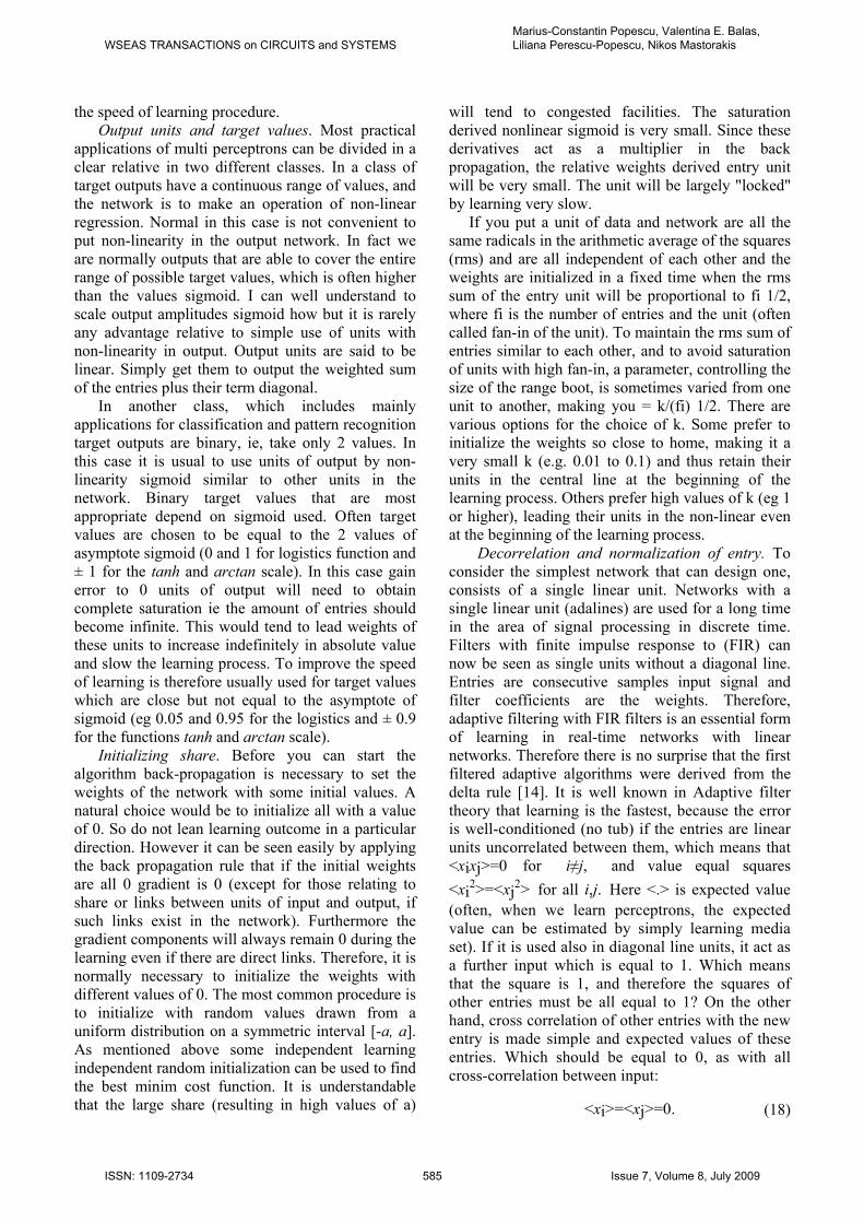
Example: We associate an input vector X=[1 –0.5] and a target vector T=[0.5 1] of size imposed by two restrictions that can be reduced to two degrees of freedom (the points W and the slopes B) of a single Adaline neuron [9]. We suggest solving the linear system of 2 equations with 2 unknowns [12]:

w+b=0.5, - 0.5w+b=1, (17)

obtaining in the end the solutions:

w= -31

and b =65

.

The Matlab program offers solutions obtained with the help of the Adaline neuron either by points or by slopes. Matlab program offers solutions obtained using Adaline neuron, either by points or by slopes [3], [7], [10], [21].

Fig. 10: The points (weight) and slopes (bias) of the

neuron identified as algebraic solutions.

5 Implementation In this section we will discuss some issues related to practical implementation perceptron and algorithm of backpropagation. Sigmoid. As I said above activation functions that are most commonly used units are multi perceptrons type sigmoid. Other types of non-linearity have been tested once but their behaviour appears to be generally inferior to those of sigmoid. In class sigmoid there are still wide choices. Feature sigmoid that seem to have the greatest influence on the performance of learning algorithm is symmetry to the home, while the logistics of the example is symmetric to a point of coordinates (0, 0.5). Symmetry to give the home a bipolar sigmoid which normally tends to lead to error surfaces better conditioned. Sigmoid as logistical curves tend to induce the narrowest error function, which weakens



the speed of learning procedure. Output units and target values. Most practical applications of multi perceptrons can be divided in a clear relative in two different classes. In a class of target outputs have a continuous range of values, and the network is to make an operation of non-linear regression. Normal in this case is not convenient to put non-linearity in the output network. In fact we are normally outputs that are able to cover the entire range of possible target values, which is often higher than the values sigmoid. I can well understand to scale output amplitudes sigmoid how but it is rarely any advantage relative to simple use of units with non-linearity in output. Output units are said to be linear. Simply get them to output the weighted sum of the entries plus their term diagonal. In another class, which includes mainly applications for classification and pattern recognition target outputs are binary, ie, take only 2 values. In this case it is usual to use units of output by non-linearity sigmoid similar to other units in the network. Binary target values that are most appropriate depend on sigmoid used. Often target values are chosen to be equal to the 2 values of asymptote sigmoid (0 and 1 for logistics function and ± 1 for the tanh and arctan scale). In this case gain error to 0 units of output will need to obtain complete saturation ie the amount of entries should become infinite. This would tend to lead weights of these units to increase indefinitely in absolute value and slow the learning process. To improve the speed of learning is therefore usually used for target values which are close but not equal to the asymptote of sigmoid (eg 0.05 and 0.95 for the logistics and ± 0.9 for the functions tanh and arctan scale). Initializing share. Before you can start the algorithm back-propagation is necessary to set the weights of the network with some initial values. A natural choice would be to initialize all with a value of 0. So do not lean learning outcome in a particular direction. However it can be seen easily by applying the back propagation rule that if the initial weights are all 0 gradient is 0 (except for those relating to share or links between units of input and output, if such links exist in the network). Furthermore the gradient components will always remain 0 during the learning even if there are direct links. Therefore, it is normally necessary to initialize the weights with different values of 0. The most common procedure is to initialize with random values drawn from a uniform distribution on a symmetric interval [-a, a]. As mentioned above some independent learning independent random initialization can be used to find the best minim cost function. It is understandable that the large share (resulting in high values of a)

will tend to congested facilities. The saturation derived nonlinear sigmoid is very small. Since these derivatives act as a multiplier in the back propagation, the relative weights derived entry unit will be very small. The unit will be largely "locked" by learning very slow. If you put a unit of data and network are all the same radicals in the arithmetic average of the squares (rms) and are all independent of each other and the weights are initialized in a fixed time when the rms sum of the entry unit will be proportional to fi 1/2, where fi is the number of entries and the unit (often called fan-in of the unit). To maintain the rms sum of entries similar to each other, and to avoid saturation of units with high fan-in, a parameter, controlling the size of the range boot, is sometimes varied from one unit to another, making you = k/(fi) 1/2. There are various options for the choice of k. Some prefer to initialize the weights so close to home, making it a very small k (e.g. 0.01 to 0.1) and thus retain their units in the central line at the beginning of the learning process. Others prefer high values of k (eg 1 or higher), leading their units in the non-linear even at the beginning of the learning process. Decorrelation and normalization of entry. To consider the simplest network that can design one, consists of a single linear unit. Networks with a single linear unit (adalines) are used for a long time in the area of signal processing in discrete time. Filters with finite impulse response to (FIR) can now be seen as single units without a diagonal line. Entries are consecutive samples input signal and filter coefficients are the weights. Therefore, adaptive filtering with FIR filters is an essential form of learning in real-time networks with linear networks. Therefore there is no surprise that the first filtered adaptive algorithms were derived from the delta rule [14]. It is well known in Adaptive filter theory that learning is the fastest, because the error is well-conditioned (no tub) if the entries are linear units uncorrelated between them, which means that <xixj>=0 for i≠j, and value equal squares <xi2>=<xj2> for all i,j. Here <.> is expected value (often, when we learn perceptrons, the expected value can be estimated by simply learning media set). If it is used also in diagonal line units, it act as a further input which is equal to 1. Which means that the square is 1, and therefore the squares of other entries must be all equal to 1? On the other hand, cross correlation of other entries with the new entry is made simple and expected values of these entries. Which should be equal to 0, as with all cross-correlation between input:

<xi>=<xj>=0. (18)



In conclusion, for a faster learning of a single unit with the diagonal line should be amended so that the process averages each component input is 0.

<xi>=0, (19)

and components are normalized and decorrelating:

<xixj>=δij, (20)

where δij is Kronecker symbol. Experience revealed that this type of processing also tends to accelerate learning for multilayer perceptrons. Setting the components of the input 0 may be made simply by adding a constant suitable for everyone. Decorelating can then be accomplished by any of orthogonal, for example, the technique describe in [15]. Finally, the normalization can be achieved by a suitable scaling of each component. The hardest step is orthogonal, many people and once you jump, by setting the average to 0 and 0 mean squares. This simplified process is usually designed as a normal entry; often increase the speed of learning networks. A technique developed to accelerate in May, involving normalization and adaptive deco relation input lines of the network is described in [16]. Common shares. In some cases one would like to constrain some of the network weights to be equal with others. This situation may occur, for example, if we are to achieve the same kind of processing in different parts of the model input. It is a situation often encountered in image processing, where some would like to detect the same feature in different parts of the input image. An example in a binary application is described in [17]. Two examples of situations with common shares will be described below, the presentation of recurrent networks. The difficulty in linking manually split shares that is payable even if the weights are initialized with the same value, derivatives of common functions of the cost of each will generally be different between them. The solution is quite simple. Assume that we collected all the weights in a weighting vector w = (W1, W2, ....) T (where T means transposed), and I share that first must be kept equal between them. These weights are not actually arguments independent of the cost function E. To maintain all arguments function is independent, should replace all of these weights with a single argument, with which they are all equal weights. Then, as derived in part of E should be calculated relative to, and not relative to all the individual weights. But

∑∑== ∂∂

=∂∂

∂∂

=∂∂ m

i i

im

i i wE

aw

wE

aE

11 (21)

Derivatives appearing in the last line can be calculated by the normal procedure of dissemination - back. In conclusion, we should calculate derivatives relative weight to each individual through the normal method, and then use the amount to update them and thus to adjust all the weights together. Also we must remember that the common weights are initialized with the same value. 6 Experimental results Inside the vector control of an induction motor it can be implemented a cvasi-PI standard fuzzy controller. The optimization criterion (absolute error integration) for such of controllers must guarantee the robustness of the system. This cvasi-PI fuzzy controller replaces the speed classic controller from the vector control schema of the driving system ([11], [12]). A fuzzy control can be implemented inside of a numerical control that involves the use of a digital signal processor DSP (for example, TMS 320C31). Taking account of the mathematical model developed in [11], [12], can be implemented a cvasi-PI standard fuzzy controller in the induction driving environment (Fig. 11).

( )20 1 2= − + +e

dJ M M k kdtω ω ω

,2= Ψm

e sr

Lq sqM p i

L (22) where M0 is the constant component part of the static torque Ms; K1 and K2 are proportional constants; Me is the electromagnetic torque ;ω is the angular speed; isq is the stator currents along the axes q; Lm is the periodical mutual inductivity between the stator and the rotor; Lm is the inductivity of the stator.

Fig. 11: Fuzzy logic controller.

Instead of the fuzzy controller [11] it is placed a neural controller which should have the learning possibility of the control surface of the fuzzy controller.



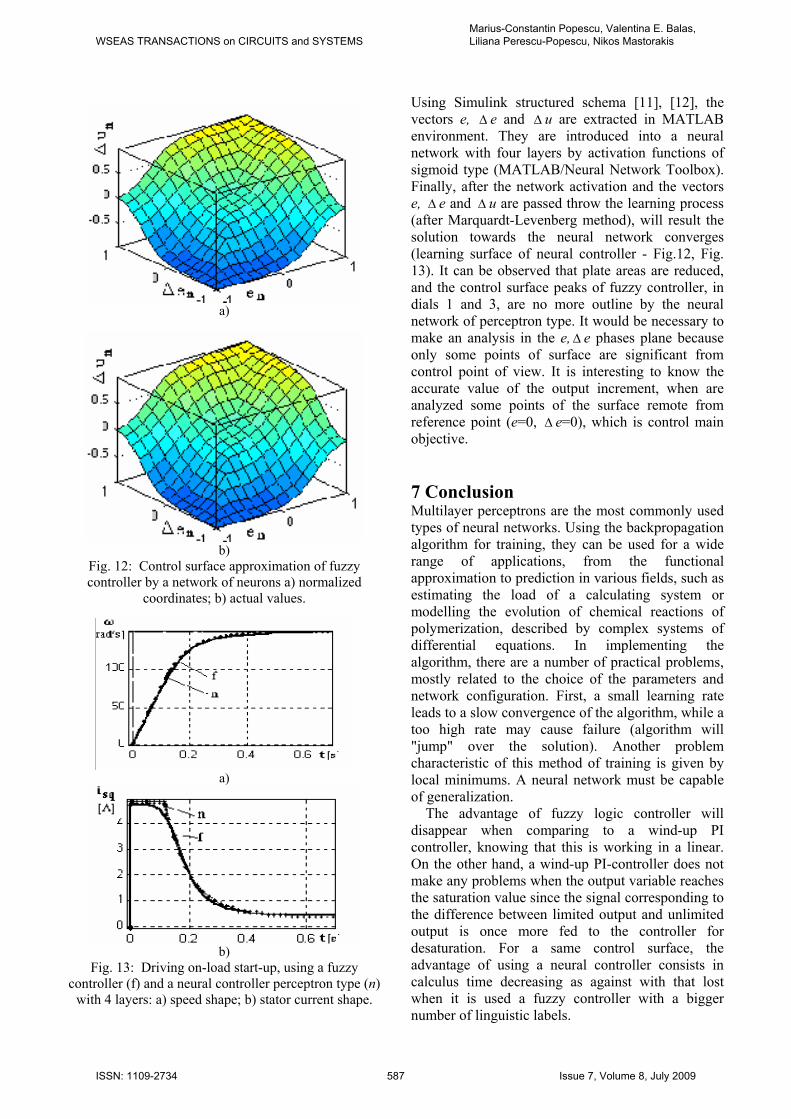
a)

b)

Fig. 12: Control surface approximation of fuzzy controller by a network of neurons a) normalized

coordinates; b) actual values.

a)

b)

Fig. 13: Driving on-load start-up, using a fuzzy controller (f) and a neural controller perceptron type (n)

with 4 layers: a) speed shape; b) stator current shape.

Using Simulink structured schema [11], [12], the vectors e, Δ e and Δ u are extracted in MATLAB environment. They are introduced into a neural network with four layers by activation functions of sigmoid type (MATLAB/Neural Network Toolbox). Finally, after the network activation and the vectors e, Δ e and Δ u are passed throw the learning process (after Marquardt-Levenberg method), will result the solution towards the neural network converges (learning surface of neural controller - Fig.12, Fig. 13). It can be observed that plate areas are reduced, and the control surface peaks of fuzzy controller, in dials 1 and 3, are no more outline by the neural network of perceptron type. It would be necessary to make an analysis in the e,Δ e phases plane because only some points of surface are significant from control point of view. It is interesting to know the accurate value of the output increment, when are analyzed some points of the surface remote from reference point (e=0, Δ e=0), which is control main objective.

7 Conclusion Multilayer perceptrons are the most commonly used types of neural networks. Using the backpropagation algorithm for training, they can be used for a wide range of applications, from the functional approximation to prediction in various fields, such as estimating the load of a calculating system or modelling the evolution of chemical reactions of polymerization, described by complex systems of differential equations. In implementing the algorithm, there are a number of practical problems, mostly related to the choice of the parameters and network configuration. First, a small learning rate leads to a slow convergence of the algorithm, while a too high rate may cause failure (algorithm will "jump" over the solution). Another problem characteristic of this method of training is given by local minimums. A neural network must be capable of generalization. The advantage of fuzzy logic controller will disappear when comparing to a wind-up PI controller, knowing that this is working in a linear. On the other hand, a wind-up PI-controller does not make any problems when the output variable reaches the saturation value since the signal corresponding to the difference between limited output and unlimited output is once more fed to the controller for desaturation. For a same control surface, the advantage of using a neural controller consists in calculus time decreasing as against with that lost when it is used a fuzzy controller with a bigger number of linguistic labels.



References [1] Almeida, L.B. Multilayer perceptrons, in

Handbook of Neural Computation, IOP Publishing Ltd and Oxford University Press, 1997.

[2] Bryson, A.E., Ho, Y.C. Applied Optimal Control, Blaisdell, New York, 1969.

[3] Curteanu, S., Petrila, C., Ungureanu, Ş., Leon, F. Genetic Algorithms and Neural Networks Used in Optimization of a Radical Polymerization Process, Buletinul Universităţii Petrol-Gaze din Ploieşti, vol. LV, seria tehnică, nr.2, pp. 85-93, 2003.

[4] Cybenko, G. Approximation by superpositions of a sigmoidal function, Math. Control, Signal Syst. 2, pp.303-314, 1989.

[5] Dumitrescu, D., Costin, H. Reţele neuronale, Teorie şi aplicaţii, Ed. Teora, Bucureşti, 1996.

[6] Haykin, S. Neural Networks: A Comprehensive Foundation, Maxmillan, IEEE Press, 1994.

[7] Leon, F., Gâlea, D., Zaharia, M. H. Load Balancing In Distributed Systems Using Cognitive Behavioural Models, Bulletin of

Technical University of Iaşi, Tome XLVIII (LII), fasc.1-4, 2002.

[8] Negnevitsky, M. Artificial Intelligence: A Guide to Intelligent Systems, Addison Wiesley, England, 2002.

[9] Popescu M.C., Hybrid neural network for prediction of process parameters in injection moulding, Annals of University of Petroşani, Electrical Engineering, Universities Publishing House, Petroşani, Vol. 9, pp.312-319, 2007.

[10] Popescu M.C., Olaru O, Mastorakis N. Equilibrium Dynamic Systems Integration Proceedings of the 10th WSEAS Int. Conf. on Automation & Information, Prague, pp.424-430, March 23-25, 2009.

[11] Popescu M.C., Modelarea şi simularea proceselor, Editura Universitaria Craiova, pp. 261-273, 2008.

[12] Popescu M.C., Petrişor A. Neuro-fuzzy control of induction driving, 6th International

Carpathian Control Congress, pp.209-214, Miskolc-Lillafured, Budapesta, 2005.

[13] Popescu M.C., Reţele neuronale şi algoritmi genetici utilizaţi în optimizarea proceselor. Sesiunea Natională de Comunicări Stiinţifice. Ediţia a IX-a. Secţiunea Matematică, Târgu-Jiu, noiembrie 24-25, 2001.

[14] Popescu M.C., Balas V., Olaru O., Mastorakis N., The Backpropagation Algorithm Functions for the Multilayer Perceptron, Proceedings of the 11th WSEAS International Conference on Sustainability in Science Engineering, pp.28-31, Timisoara, Romania, may 27-29, 2009.

[15] Popescu M.C,, Olaru O., Mastorakis N., Equilibrium Dynamic Systems Intelligence, WSEAS Transactions on Information Science and Applications, Issue 5, Volume 6, pp.725-735, May 2009.

[16] Popescu M.C., Olaru O, Mastorakis N. Equilibrium Dynamic Systems Integration, Proceedings of the 10th WSEAS Int. Conf. on Automation & Information (ICAI '09), March 23-25, 2009.

[17] Popescu M.C., Petrişor A., Drighiciu A., Fuzzy Control Algorithm Implementation using LabWindows – Robot, WSEAS Transactions on Systems Journal, Issue 1, Volume 8, pp.117-126, January 2009,

[18] Principe, J.C., Euliano, N.R., Lefebvre, W.C. Neural and Adaptive Systems. Fundamentals Through Simulations, John Wiley & Sons, Inc, 2000.

[19] Rumelhart, D.E., Hinton, G.E., Williams, R.J. Learning representations by backpropagating errors, Nature 323, pp.533-536, 1986.

[20] Silva, F.M., Almeida, L.B. Acceleration techniques for the backpropagation algorithm in L.B. Almeida, C.J. Wellekens (eds.), Neural Networks, Springer, Berlin, pp.110–19, 1990.

[21] Werbos, P.J. The Roots of Backpropagation, John Wiley & Sons, New York, 1974.



multilayer perceptron and neural networks - wseas · multilayer perceptron and neural networks...

Documents