1

MULTILEVEL ANALYSIS IN THE STUDY OF CRIME AND JUSTICE

“The most pervasive fallacy of philosophic thinking goes back to neglect of context”

(John Dewey, 1931)

Neither criminal behavior nor society’s reaction to it occurs in a social vacuum – for this reason

criminology as a discipline is inherently a multilevel enterprise. Individual criminal behavior is

influenced by larger social, political and environmental factors, as are the decisions of various actors in

the criminal justice system. Classroom and school characteristics affect adolescent development,

misconduct and delinquency (Beaver et al. 2008; Osgood and Anderson, 2004; Stewart, 2003). Family

and neighborhood characteristics influence the likelihood of victimization and offending as well as post-

release recidivism and fear of crime (Nieuwbeerta et al., 2008; Wilcox et al., 2007; Lauritsen and

Schaum, 2004; Kubrin and Stewart, 2006; Wyant, 2008; Lee and Ulmer, 2000). Police department,

precinct and neighborhood factors affect police arrest practices, use of force and clearance rates (Smith,

1986; Sun et al. 2008; Lawton, 2007; Pare et al. 2007; Eitle et al. 2005; Terrill and Reisig, 2003). Judge

characteristics and court contexts affect individual punishment decisions (Britt, 2000; Ulmer and Johnson,

2004; Johnson, 2006; Wooldredge, 2007) and prison environments are tied to inmate misconduct,

substance use and violence (Camp et al. 2003; Gillespie 2005; Huebner, 2003; Wooldredge et al. 2001).

Although these examples cover a diverse array of criminological topics, they all share a common

analytical quality – each involves data that are measured across multiple units of analysis. When this is

the case, multilevel models offer a useful statistical approach for studying diverse issues in crime and

justice. As Table 1 demonstrates, recent years have witnessed an abundance of multilevel studies across a

variety of topics in criminology and criminal justice.

This chapter provides a basic introduction to the use of multilevel statistical models in the field.

It begins with a conceptual overview explaining what multilevel models are and why they are necessary.

It then provides a statistical overview of basic multilevel models, illustrating their application using

punishment data from federal district courts. The chapter concludes with a discussion of advanced

applications and common concerns that arise in the context of multilevel research endeavors.

2

CONCEPTUAL OVERVIEW

Multilevel statistical models are necessitated by the fact that social relationships exist at several

different levels of analysis that jointly influence outcomes of interest. Smaller units of analysis are often

“nested” within one or more larger units of analysis. For instance, students are nested within classrooms

and schools, offenders and victims are both nested within family and neighborhood environments, and

criminal justice personnel are nested within larger community and organizational contexts. In each of

these cases, the characteristics of some larger context are expected to influence individual behavior. This

logic can be extended to any situation involving multiple levels of analysis including but not limited to

individuals, groups, social networks, neighborhoods, communities, counties, states and even countries.

Moreover, longitudinal research questions often involve multilevel data structures, with repeated

measures nested within individuals or with observations nested over time (e.g. Horney et al. 1995;

Slocum et al. 2005; Rosenfeld et al. 2007). Other common applications of multilevel analysis include

twin studies with paired or clustered sibling dyads (e.g. Wright et al. 2008; Taylor et al. 2002) and meta-

analyses that involve multiple effect sizes nested within the same study or dataset (e.g. Raudenbush,

1984; Goldstein et al. 2000). Regardless of the level of aggregation or “nesting,” though, the important

point is that criminological enterprises often involve data that span multiple levels of analysis. In fact,

given the complexity of our social world, it can be difficult to identify topics of criminological interest

that are not characterized by multiple spheres of social influence. When these multiple influences are

present, multilevel statistical models represent a useful and even necessary tool for analyzing a broad

variety of criminological research questions.

A MODEL BY ANY OTHER NAME?

Given the complexity surrounding multilevel models, it is useful to distinguish up front what can

sometimes be a confusing and inexact argot. Various monikers are used to describe multilevel statistical

models (e.g. multilevel models, hierarchical models, nested models, mixed models). Although this

nomenclature is often applied interchangeably, there can be subtle but important differences in these

designations. Multilevel modeling is used here as a broad, all-encompassing rubric for statistical models

3

that are explicitly designed to analyze and infer relationships for more than one level of analysis.1 The

language of multilevel models is further complicated by the fact that there are various different software

packages that can be used to estimate multilevel models, some of which are general statistical packages

(e.g. SAS, STATA) and others that are specialized multilevel programs (e.g. HLM, MLwin, aML).2

Additional confusion may derive from the fact that scholars often use terminology such as

ecological, aggregate and contextual effects interchangeably despite important differences in their

meaning. Ecological effects, or group-level effects, can refer to any group level influence that is

associated with the higher level of analysis. Group level effects can take several forms. First, aggregate

effects (sometime referred to as analytical or derived variables) are created by aggregating individual

level characteristics up to the group level of analysis (e.g. percent male in a school). These are sometimes

distinguished from structural effects that are also derived from individual data but capture relational

measures among members within a group (e.g. density of friendship networks) (see Luke, 2004: 6). To

complicate matters, when individual level data are aggregated to the group level they can exert two

distinct types of influence – first, they can exert compositional effects which reflect group differences that

are attributable to variability in the constitution of the groups – between-group differences may simply

reflect the fact that groups are made up of different types of individuals. Second they can exert contextual

effects which represent influences above and beyond differences that exist in group composition.

Contextual effects are sometimes referred to as emergent properties because the collective exerts a

synergistic influence that is unique to the group aggregation and which is not present in the individual

1 Hierarchical or nested models, for instance, technically refer to data structures involving exact nesting of smaller

levels of analysis within larger units. Multilevel data, however, can also be non-nested, or “cross-classified”, in

ways that do not follow a neat hierarchical ordering. Data might be nested within years and within states at the same

time, for example, with no clear hierarchy to “year” and “state” as levels of analysis (Gelman and Hill, 2007: 2).

Similarly, adolescents might be nested within schools and neighborhoods with students from the same neighborhood

attending different schools. Although these cases clearly involve multilevel data, they are not hierarchical in a

technical sense. Similarly, “mixed models” technically refer to statistical models containing both “fixed” and

“random” effects. Although this often is the case in multilevel models, it is not necessarily the case, so the broader

rubric multilevel modeling is preferred to capture the variety of models designed to incorporate data across multiple

units of analysis. 2 A useful and detailed review of the strengths and limitations of numerous software programs that provide for the

estimation of multilevel models is provided by the Centre for Multlevel Modeling at the University of Bristol at

http://www.cmm.bris.ac.uk/learning-training/multilevel-m-software/index.shtml.

4

constituent parts.3 Although the term “contextual effect” is sometimes used as a broader rubric for any

group level influence, the narrower definition provided here is often useful for distinguishing among

types of ecological influences that can be examined in multilevel models. Finally, global effects refer to

structural characteristics of the collective itself that are not derived from individual data but rather reflect

measures that are specific to the group (e.g. physical dilapidation of the school). These and other

commonly used terms in multilevel analysis are summarized in Table 2.4

THEORETICAL RATIONALES FOR MULTILEVEL MODELS

The need for multilevel statistical models is firmly rooted in both theoretical and methodological

rationales. Multilevel models are extensions of traditional regression models that account for the

structuring of data across aggregate groupings, that is, they explicitly account for the nested nature of data

across multiple levels of analysis. Because our social world is inherently multilevel, theoretical

perspectives that incorporate multiple levels of influence in the study of crime and justice are bound to

improve our ability to explain both individual criminal behavior and society’s reaction to it.

Figure 1 presents a schematic of a hypothetical study examining the influence of low self-control

on delinquency in a sample of high school students. Imagine that self-control is measured at multiple

time points for the same sample of students. In that case, multiple measures of self-control would be

nested within individual students, and individual students would be nested within classrooms which are

nested within schools. The lowest level of analysis would be within-individual observations of self-

control, and the highest level of analysis would be school-level characteristics. Ignoring this hierarchical

data structuring, then, is likely to introduce omitted variable bias of a large-scale theoretical nature.

3 Philosophical discourse on emergent properties dates all the way back to Aristotle but was perhaps most lucidly

applied by John Stuart Mill. He argued that the human body in its entirety produces something uniquely greater

than its singular organic parts, stating that “To whatever degree we might imagine our knowledge of the properties

of the several ingredients of a living body to be extended and perfected, it is certain that no mere summing up of the

separate actions of those elements will ever amount to the action of the living body itself” (Mill, 1843). Contextual

effects models have long been applied in sociology and related fields (e.g. Firebaugh, 1978; Blalock, 1984), but

these applications differ from multilevel models in that the latter are more general formulations that specifically

account for residual correlation within groups and explicitly provide for examination of the causes of between-group

variation in outcomes. 4 Table 2 is partially adapted from Diez Roux (2002) which contains a more detailed and elaborate glossary of many

of these terms.

5

Moreover, many theoretical perspectives explicitly argue that micro-level influences will vary

across macro-social contexts. For instance, racial group threat theories (Blumer, 1958; Liska, 1992)

predict that the exercise of formal social control will vary in concert with large or growing minority

populations. Testing theoretical models that explicitly incorporate variation in micro-effects across

macro-theoretical contexts therefore offers an important opportunity to advance criminological

knowledge. Assuming that theoretical influences operate at a single level of analysis is likely to provide a

simplistic and incomplete portrayal of the complex criminological social world.

Moreover, inferential problems can emerge when data are used to draw statistical conclusions

across levels of analysis. For instance, in his classic study of immigrant literacy, Robinson (1950)

examined the correlation between aggregate literacy rates and the proportion of the population that was

immigrant at the state level. He found a substantial positive correlation between percent immigrant and

the literacy rate (r=.53). Yet when individual level data on immigration and literacy were separately

examined, the correlation reversed and became negative (r=-.11). Although individual immigrants had

lower literacy, they tended to settle in states with high native literacy rates thus confounding the

individual and aggregate relationships. This offers an example of the ecological fallacy, or erroneous

conclusions involving individual relationships that are inferred from aggregate data. As Peter Blau (1960:

179) suggested, aggregate studies are limited because they cannot “separate the consequences of social

conditions from those of the individual's own characteristics for his behavior, because ecological data do

not furnish information about individuals except in the aggregate.”

The same mistake in statistical inference can occur in the opposite direction. The atomistic (or

individualistic) fallacy occurs when aggregate relationships are mistakenly inferred from individual level

data. Because associations between two variables at the individual level may differ from associations for

analogous variables at a higher level of aggregation, aggregate relationships cannot be reliably inferred

from individual level data. For instance, social disorganization theory would predict that crimes rates

across neighborhoods are related to mobility rates because high population turnover reduces informal

social control at the neighborhood level. Because this prediction refers to neighborhoods as the unit of

6

analysis, though, one would risk serious inferential error testing this group-level hypothesis with

individual level data. For instance, one could not test the theory by examining whether or not individuals

who move residences have higher criminal involvement. To do so would be to commit the atomistic

fallacy. This reflects the fact that variables aggregated up from individual level data often have unique

and independent contextual effects. Moving to a new residence represents a different causal pathway than

living in a neighborhood with high rates of residential mobility.5

Because of the inherent difficulties in making statistical inferences across different levels of

analysis, a preferred approach is to use multilevel analytic procedures to simultaneously incorporate

individual and group level causal processes. Multilevel models explicitly provide for this type of

statistical analysis. The difficulty is in distinguishing among the different types of individual and

ecological influences that are of theoretical interest and then specifying the statistical model to properly

estimate these effects.

MULTILEVEL MODELING AND HYPOTHESIS TESTING

There are also persuasive statistical reasons for engaging in multilevel modeling, such as

providing improved parameter estimates, corrected standard errors, and conducting more accurate

statistical significance tests. Utilizing traditional regression models for multilevel data presents several

problems. Figure 2 presents a second example of hierarchical data where individual criminal offenders

are nested within judges and county courts. Because several offenders are sentenced by the same judge

and several judges share the same courtroom environment, statistical dependencies are likely to arise

among clustered observations. When individual data is nested within aggregate groups, observations

within clusters are likely to share unaccounted-for similarities. If, for instance, some judges are “hanging

judges” while others are “bleeding-heart liberals,” then offenders sentenced by the former will have

sentences that are systematically harsher than offenders sentenced by the latter. Statistically speaking, the

5 Two related but distinct problems of causal inference are the psychologistic fallacy, which can occur when

individual level data are used to draw inferences without accounting for confounding ecological influences, and the

sociologistic fallacy which may arise from the failure to consider individual level characteristics when drawing

inferences about the causes of group variability. The pyschologistic fallacy results from a failure to adequately

consider contextual effects, whereas the sociologistic fallacy results from a failure to capture compositional effects.

7

residual errors will be correlated, systematically falling above the regression line for the first judge and

below it for the second. Because one of the assumptions of ordinary regression models is that residual

errors are independent, such systematic clustering would violate this core model assumption. The

consequence of this violation is that standard errors will be underestimated by the ordinary regression

model. Statistical significance tests will therefore be too liberal, risking Type I inferential errors in which

the null hypothesis is falsely rejected even when true in the population. Multilevel statistical models are

needed to account for statistical dependencies that occur among clusters of hierarchically organized data.6

A related problem is that statistical signifiance tests in ordinary regression models utilize the

wrong degrees of freedom for ecological predictors in the model. Traditional regression models fail to

account for the fact that hierarchically structured data are characterized by different sample sizes at each

level of analysis. For example, with data on 1,000 students nested within 50 schools, there would be an

individual level sample size of 1,000 observations but a school level sample size of only 50 observations.

This means that statistical significance tests for school-level predictors need to be based on degrees of

freedom that reflect the number of schools in the data, not the number of students. Statistical significance

tests in ordinary regression models fail to recognize this important distinction. The consequence is that

the amount of statistical power available for testing school-level predictors will be exaggerated. The

number of degrees of freedom for statistical significance tests needs to be adjusted for the number of

aggregate units in the data – multilevel models provide these adjustments.

A third advantage of multilevel models over ordinary regression models is that they allow for the

modeling of heterogeneity in regression effects. The single-level regression model assumes de facto that

individual predictors exert the same effect in each aggregate grouping. Multilevel models, on the other

hand, explicitly allow for variation in the effects of individual predictors across higher levels of analysis.

6 A simpler alternative to the full multilevel model is to estimate an ordinary regression using robust standard errors

that are adjusted for the clustering of observations across level 2 units. For example, STATA provides a “cluster”

command option that adjusts standard errors for residual dependency. This can be a useful approach when the goal

is simply to “control” for clustering, but beyond that it does not provide the same advantages of the multilevel

model. Another option is to control for group-level variation using a “fixed effects” model that includes dummy

variables for each level 2 unit in the data. This is a useful approach for removing the intraclass correlation due to

group dependency, but it precludes examination of between-group differences.

8

Ulmer and Bradley, (2006), for instance, have argued that the effect of trial conviction on criminal

sentence varies across courts. This proposition is illustrated in Figure 3 using federal punishment data for

a random sample of 8 districts courts. The ordinary regression model would constrain the effect of trial

conviction to be uniform across courts, but Figure 3 clearly suggests variation in this effect across courts.

Multilevel analysis allows for this type of variation to be explicitly incorporated into the statistical model,

providing the researcher with a useful tool for better capturing the real-world complexity that is likely to

characterize individual influences across criminological contexts.

Other advantages that also characterize multilevel models are that they provide for convenient

and accurate tests of cross-level interactions, or moderating effects that involve both individual and

ecological variables. For example, the influence of individual socioeconomic status on delinquency

might depend on the socioeconomic composition of the school. This conditional relationship could be

directly investigated by specifying a cross-level interaction between an individual’s SES and the mean

SES at the school level.

One final statistical advantage of multilevel models is that they are able to simultaneously

incorporate information both within and between groups in order to provide optimally-weighted group

level estimates. This is accomplished by combining information from the group itself with information

from other similar groups in the data, and it is particularly useful when some groups have relatively few

observations. Because groups with smaller sample sizes will have less reliable group means, some

regression to the overall grand mean is expected. Utilizing a Bayesian estimation approach, the

multilevel model shifts the within group mean toward the mean for other groups. The more reliable the

group mean, the more heavily it is weighted; the less reliable (and the less variability across groups), the

more the estimate is shifted toward the overall grand mean for all groups in the data. Thus estimates for

specific groups are based not only on their own within-group data, but also on data from other groups.

This process is sometimes referred to as “borrowing power” because within-group estimates benefit from

information on other groups, and the estimates themselves are sometimes called “shrinkage estimates”

because they “shrink” individual group means toward the grand mean for all groups. The end result is

9

that group level estimates are optimally weighted to reflect information both within and between groups

in the data.7

Multilevel models, then, provide numerous analytical and statistical advantages over ordinary

regression approaches when data are nested across levels of analysis. By providing for the simultaneous

inclusion of individual and group level information, they better specify the complex relationships that

often characterize our social world, and they help overcome common problems of statistical inference

associated with reliance on single-level data. Moreover, multilevel models correct for the problematic

clustering of observations that may occur with nested data, they provide a convenient approach for

modeling both within and between group variability in regression effects, and they offer improved

parameter estimates that simultaneously incorporate within and between group information. The

remaining discussion provides a basic statistical introduction to the multilevel model along with examples

illustrating its application to the study of criminal punishment in federal court.

STATISTICAL OVERVIEW

Multilevel models are simple extensions of ordinary regression models, which account for the

nesting of data within higher-order units. It is therefore useful to begin with an overview of the basic

regression model in order to demonstrate how the multilevel adaptation builds upon and extends it to the

case of multilevel data. For illustrative purposes, examples are provided using United States Sentencing

Commission (USSC) data on a random sample of 25,000 convicted federal offenders nested within 89

federal district courts across the U.S.8

FROM ORDINARY REGRESSION TO MULTILEVEL ANALYSIS

7 The following equation provides the formula for this weighting process (Raudenbush and Bryk, 2002: 46):

( ) 00

* ˆ1ˆ γλλβ jjjj Y −+= •

where *ˆjβ is the group estimate, which is a product of the individual group mean

jY• weighted by its reliability

jλ ,

plus the overall grand mean 00γ̂ weighted by the complement of the reliability ( )

jλ−1 . If the reliability of the group

mean is one, the weighted estimate reduces to the group mean; if it is zero, it reduces to the grand mean. The more

reliable the group mean, then, the more it counts in the multilevel estimate. When the assumptions of the multilevel

model are met, this provides the most precise and most efficient estimator of the group mean. 8 These data are drawn from fiscal years 1997 to 2000 and are restricted to the 89 federal districts and 11 circuit

courts within the U.S., with the District of Columbia excluded because it has its own district and circuit court. For

more information on the USSC data see Johnson et al. (2008).

10

When faced with multilevel data (e.g. lower-level data that is nested within some higher-level

grouping), ordinary regression approaches can take three basic forms. First, individual data can be pooled

across groups and analyzed without regard for group structure. This approach ignores important group-

level variability and often violates key assumptions of OLS regression such as independent errors.

Second, separate un-pooled analyses can be conducted within each group. This approach can be useful

for examining between-group variability, but it requires relatively large samples for each group and it is

cumbersome when the number of groups becomes large. Third, aggregate analysis can also be conducted

at the group level alone, but this approach ignores within-group variability and requires a relatively large

number of groups for analysis. In each of these cases, traditional regression approaches are unable to

incorporate the full range of information available at both the individual and group level of analysis and

they may violate important assumptions of the single-level ordinary regression model.

For illustrative purposes, the ordinary regression model is presented in Equation 1:

(1)

where Yi is a continuous dependent variable, β0 is the model intercept, β1 is the effect of the independent

variable Xi for individual i and ri is the individual level residual error term. Two key assumptions of the

linear regression model are that the relationship between Xi and Yi can be summarized with a single linear

regression line and that all of the residual error terms for individuals in the data are statistically

independent of one another. Both of these assumptions are likely to be violated with multilevel data, the

first because the effect of Xi on Yi might vary by group and the second because individuals within the

same group are likely to share unaccounted-for similarities.

Failure to account for the nesting of observations can result in “false power” at both levels of

analysis. False power occurs because there is typically less independent information available when

observations are clustered together. Consider the difference between a) data from 50 schools with 20

students each, versus b) data from 1,000 schools with one student each. The number of students is the

same, but if students share similarities within schools, each student provides less unique information in

the first sample than in the second. Moreover, there is more unique school level data in the second

iii rXY ++= 10 ββ

11

sample than in the first. Because ordinary regression models ignore the clustering of individuals within

schools, they treat both samples as equivalent. The consequence of this is that the amount of statistical

power for the first sample is artificially inflated at both the individual and school level of analysis.

Moreover, standard errors for the first sample will be underestimated and significance tests will be too

liberal if there are unaccounted-for similarities among students within schools.

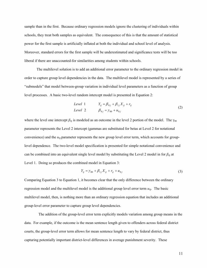
The multilevel solution is to add an additional error parameter to the ordinary regression model in

order to capture group level dependencies in the data. The multilevel model is represented by a series of

“submodels” that model between-group variation in individual level parameters as a function of group

level processes. A basic two-level random intercept model is presented in Equation 2:

jj

ijijjjij

uLevel

rXYLevel

0000

10

2

1

+=

++=

γβ

ββ (2)

where the level one intercept β0j is modeled as an outcome in the level 2 portion of the model. The γ00

parameter represents the Level 2 intercept (gammas are substituted for betas at Level 2 for notational

convenience) and the u0j parameter represents the new group level error term, which accounts for group-

level dependence. The two-level model specification is presented for simple notational convenience and

can be combined into an equivalent single level model by substituting the Level 2 model in for β0j at

Level 1. Doing so produces the combined model in Equation 3:

(3)

Comparing Equation 3 to Equation 1, it becomes clear that the only difference between the ordinary

regression model and the multilevel model is the additional group level error term u0j. The basic

multilevel model, then, is nothing more than an ordinary regression equation that includes an additional

group-level error parameter to capture group level dependencies.

The addition of the group-level error term explicitly models variation among group means in the

data. For example, if the outcome is the mean sentence length given to offenders across federal district

courts, the group-level error term allows for mean sentence length to vary by federal district, thus

capturing potentially important district-level differences in average punishment severity. These

jijijjij urXY 0100 +++= βγ

12

differences are illustrated in Figure 4, where Panel A shows the mean sentence length pooled across a

sample of ten federal districts, and Panel B shows the mean sentence length disaggregated by federal

district. The figure indicates that average punishments vary across federal courts. For instance, the mean

sentence length in the Northern District of Florida is about twice the average sentence in the District of

Delaware. Important differences in variability in punishment also exist across federal districts, with the

standard deviation in the Western District of Oklahoma being more than twice that in the Southern

District of California. These group level variations are captured by the incorporation of the group-level

error term in the multilevel statistical model, resulting in standard errors and statistical significance tests

that are properly adjusted for the nesting of individual cases within aggregate district court groupings.

BUILDING THE MULTILEVEL MODEL

Despite its conceptual simplicity, multilevel analysis adds a layer of analytical complexity that

can quickly become cumbersome when applied to research questions involving multiple predictors across

multiple levels of analysis. For this reason it is essential to build the multilevel model carefully from the

ground up. There are several types of multilevel models that vary in complexity, including 1)

unconditional models, 2) random intercept models, 3) random coefficient models and 4) cross-level

interaction models – each adds an additional layer of complexity and provides additional information in

the multilevel analysis.

THE UNCONDITIONAL MODEL

The first step in multilevel analysis is to investigate the necessity of using a multilevel model.

This is both a theoretical and statistical question. First, the research question should always dictate the

methodology. Some research questions that involve multiple levels of data may be answerable with

simpler and more parsimonious analytical approaches. So called “fixed effects” models, for instance, can

be a simple and effective way of removing between-group variation. Including a series of dummy

variables for level 2 units parcels out the level 2 variation and corrects for any intraclass correlation

among nested observations. Before adopting a multilevel model, then, it is important to first make sure

the research question necessitates multilevel analysis. Despite its advantages the multilevel model is not

13

always necessary, nor ideal. For instance, a minimum number of aggregate groupings is generally needed

for multilevel analysis because a sufficient number of level 2 units is required for higher order statistical

significance tests.9 It is also useful to begin by testing for the presence of correlated errors before turning

to multilevel analysis. This can be done by estimating an ordinary regression, saving the residuals, and

then conducting an analysis of variance to investigate whether or not the residuals are significantly related

to group membership. Significant results provide evidence that the ordinary regression assumption of

independent errors is violated by the nested structure of the data.

The necessity of multilevel analysis can be further investigated through the unconditional or null

model. This model is referred to as “unconditional” because it includes no predictors at any level of

analysis, so it provides a predicted value for the mean which is not conditional on any covariates. It is

summarized in Equation 4:

jj

ijjij

uLevel

rYLevel

0000

0

2

1

+=

+=

γβ

β (4)

where ijY is a continuous outcome for individual i in group j, estimated by the overall intercept j0β plus

an individual-level error term, ijr . At level 2 of the model, the intercept j0β is modeled as a product of a

level 2 intercept 00γ plus a group-level error term, ju0 . The unconditional model decomposes the total

variance in the outcome into two parts – an individual variance, captured by the individual-level error

term, and a group variance, captured by the group-level error term. The unconditional model is therefore

useful for investigating the amount of variation that exists within versus between groups. One way to

9 Scholars disagree on this point. Some advocate using multilevel models in any situation involving nested data (e.g.

Gelman and Hill, 2007) while others caution its use in analyses involving relatively few level 2 units (e.g. Snidjers

and Bosker, 1999: 44). Although there does not seem to be widespread consensus on what constitutes a sufficient

number of groups (in part because the number of observations per grouping also matters), a general rule of thumb

might be to require about a dozen or so groupings before turning to multilevel analysis, at least for analyses that

include level 2 predictors. This issue in part reflects concerns over statistical power in multilevel analysis, which is

a product of several factors including the number of clusters, the number of observations per cluster, the strength of

the intraclass correlation and the effect sizes for level 2 variables in the model, all of which will affect the decision

to employ multilevel analysis. A useful optimal design software program for conducting power analysis with

multilevel data is available at: http://sitemaker.umich.edu/group-based/optimal_design_software.

14

quantify this is to calculate the intraclass correlation coefficient (ICC), which represents the proportion of

the total variance that is attributable to between-group differences. The ICC is represented by Equation 5:

( )002

00

τσ

τρ

+= (5)

where 00τ is the between-group variance estimated by the ju0 parameter and 2σ is the within-group

variance estimated by the ijr parameter in Equation 4. The intraclass correlation is the ratio of between

group variance to total variance in the outcome. Larger ICCs indicate that a greater proportion of the total

variance in the outcome is due to between-group differences.10

It is important to begin any multilevel

analysis by estimating the unconditional model. It provides an assessment of whether or not significant

between-group variation exists – if it does not, then multilevel analysis is unnecessary – and it serves as a

useful baseline model for evaluating explained variance in subsequent model specifications.

Table 3 presents the results from an unconditional model examining sentence length for a random

sample of federal offenders nested within U.S. district courts. The results are broken into two parts, one

for the “fixed effects”, which report the unstandardized regression coefficients, and one for the “random

effects”, which report the variance components for the model. The overall intercept is 52.5 months

indicating that the average federal sentence in this sample is just under 5 years. The level 1 variance

provides a measure of within-district variation in sentence lengths and the level 2 variance provides an

analogous measure for between-district variation. The significance test associated with the level 2

variance component indicates there is significant between district variation in sentences – sentence

lengths vary significantly across federal district courts. Notice that the significance test uses degrees of

freedom for the number of level 2 rather than level 1 units; it provides preliminary evidence that districts

10

It is common in multilevel analysis for between-group variation to represent a relatively small proportion of the

total variance, however, as Liska (1990) argues, this does not indicate that between group variation is unimportant.

15

matter in federal punishment, although as Luke (2004) points out, significance tests for variance

components should always be interpreted cautiously.11

In order to get a sense of the magnitude of inter-district variation in punishment, the intraclass

correlation coefficient (ICC) can be calculated and the random effects can be assessed in combination

with the fixed effects in Table 3. The level 2, or between group, variance is 00τ = 267 and the within-

group, or individual variance is 2σ = 4,630. Plugging these values into Equation 5 gives an ICC equal to

.055. This indicates that 5.5% of the total variation in sentence length is attributable to between-district

variation in sentencing. Similarly, the standard deviation for the between group variance component can

be added and subtracted to the model intercept to provide a range of values for average sentences among

districts. Adding and subtracting 16 months gives a range between 36.2 and 68.9 months, so the average

sentence varies between 3 years and 5 ¾ years for one standard deviation (i.e. about two-thirds) of federal

district courts. The significance test, intraclass correlation and range of average sentences all suggest

important between-group variation, indicating that multilevel analysis is appropriate in this instance.

THE RANDOM INTERCEPT MODEL

The second type of multilevel model adds predictor variables to the unconditional model and is

referred to as a random intercept model because it allows the intercept to take on different values for each

level 2 unit in the data. There are three types of random intercept models – models that include only level

1 predictors, models that include only level 2 predictors, and models that include both level 1 and level 2

predictors. In the first model, the focus of the multilevel analysis is on controlling for statistical

dependence in clustered observations. In the second the focus is on estimating variation in group means

as a function of group-level predictors, and in the third, the focus in on estimating the joint influence of

both level 1 and level 2 predictors. The type of random intercept model will depend on the research

11

Variances are bounded by zero so they are not normally distributed and they are usually expected to take on non-

zero values anyway so it is not always clear what a significant variance means. Although significance tests for

variance components can provide a useful starting point, then, they should be used judiciously. It is much more

useful to interpret the substantive magnitude of the variance component rather than just its statistical significance.

16

question of interest, but it is often useful to begin by estimating the model with only level 1 predictors.

This model is presented in Equation 6:

jj

ijijjjij

uLevel

rXYLevel

0000

10

2

1

+=

++=

γβ

ββ (6)

where ijX represents an individual level predictor added to the unconditional model in Equation 4. Again

the level 2 equation models the level 1 intercept j0β as a product of both the overall mean intercept, 00γ ,

and a unique level 2 error term, ju0 . Substantively this means that the model intercept is allowed to vary

randomly across level 2 units; each level 2 unit in the sample has its own group-specific intercept, just as

if separate regressions were estimated for each group in the data.

Table 4 presents the results from a model examining the impact of the severity of the offense on

the final sentence. In this model offense severity is centered around its grand mean (see discussion of

centering below) and added to the level 1 portion of the model as a predictor of sentence length. j1β in

Equation 6 represents the effect of offense severity, ijX , on the length of one’s sentence in federal court.

It is interpreted just as it would be in an ordinary regression model – each one unit increase in offense

severity increases one’s sentence length by 5.56 months. The average sentence is also allowed to vary by

federal district, however. This is reflected by the level 2 variance component ju0 in Table 4. Both

variance components now represent residuals, or left-over variation that is unaccounted for by the model.

Notice that the deviance statistic is reduced from the unconditional to the conditional model, indicating

increased model fit.12

To better quantify the model fit, it is often useful to calculate proportionate

12

The deviance statistic is equal to -2 times the natural log of the likelihood function and serves as a measure of lack

of fit between the model and the data – the smaller the deviance the better the model fit. The inclusion of additional

predictors will decrease the model deviance, and although the deviance is not directly interpretable it is useful for

comparing alternative model specifications to one another (Luke, 2004). The difference in deviance statistics for

two models is distributed as a chi-square distribution with degrees of freedom equal to the difference in the number

of parameters in the two models. Multilevel models are typically fit with maximum likelihood estimation but this

can be done using either full maximum likelihood (ML) or restricted maximum likelihood (REML). Both estimators

will produce identical estimates of the fixed effects, but REML will produce variance estimates that are less biased

than ML when the number of level 2 units is relatively small (see Kreft and DeLeeuw, 1998: 131-133; Snidjers and

Bosker,1999: 88-90). REML is useful for testing two nested models that differ only in their random effects (e.g. an

17

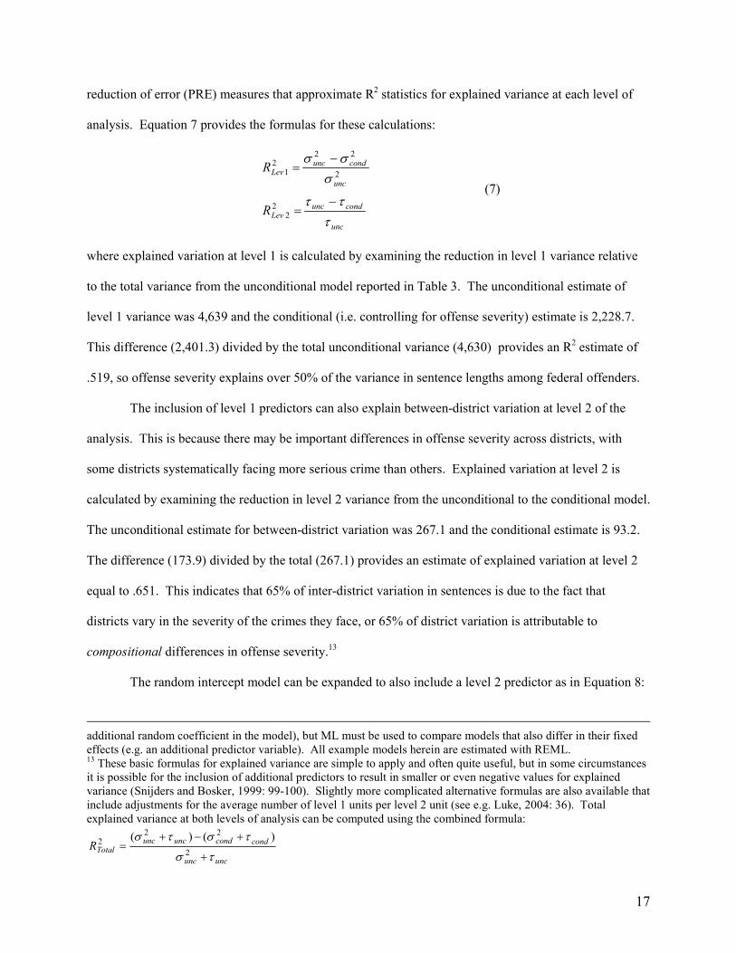
reduction of error (PRE) measures that approximate R2 statistics for explained variance at each level of

analysis. Equation 7 provides the formulas for these calculations:

unc

conduncLev

unc

conduncLev

R

R

τ

ττ

σ

σσ

−=

−=

22

2

222

1

(7)

where explained variation at level 1 is calculated by examining the reduction in level 1 variance relative

to the total variance from the unconditional model reported in Table 3. The unconditional estimate of

level 1 variance was 4,639 and the conditional (i.e. controlling for offense severity) estimate is 2,228.7.

This difference (2,401.3) divided by the total unconditional variance (4,630) provides an R2 estimate of

.519, so offense severity explains over 50% of the variance in sentence lengths among federal offenders.

The inclusion of level 1 predictors can also explain between-district variation at level 2 of the

analysis. This is because there may be important differences in offense severity across districts, with

some districts systematically facing more serious crime than others. Explained variation at level 2 is

calculated by examining the reduction in level 2 variance from the unconditional to the conditional model.

The unconditional estimate for between-district variation was 267.1 and the conditional estimate is 93.2.

The difference (173.9) divided by the total (267.1) provides an estimate of explained variation at level 2

equal to .651. This indicates that 65% of inter-district variation in sentences is due to the fact that

districts vary in the severity of the crimes they face, or 65% of district variation is attributable to

compositional differences in offense severity.13

The random intercept model can be expanded to also include a level 2 predictor as in Equation 8:

additional random coefficient in the model), but ML must be used to compare models that also differ in their fixed

effects (e.g. an additional predictor variable). All example models herein are estimated with REML. 13

These basic formulas for explained variance are simple to apply and often quite useful, but in some circumstances

it is possible for the inclusion of additional predictors to result in smaller or even negative values for explained

variance (Snijders and Bosker, 1999: 99-100). Slightly more complicated alternative formulas are also available that

include adjustments for the average number of level 1 units per level 2 unit (see e.g. Luke, 2004: 36). Total

explained variance at both levels of analysis can be computed using the combined formula:

uncunc

condconduncuncTotalR

τσ

τστσ

+

+−+=

2

222 )()(

18

jjj

ijijjjij

uWLevel

rXYLevel

001000

10

2

1

++=

++=

γγβ

ββ (8)

Group mean differences in the intercept, j0β , are now modeled as a product of a group-level predictor,

jW , with 01γ representing the effect of the level 2 covariate on the outcome of interest. Level 2 predictors

can take several forms including aggregate, structural or global measures (see Table 2). Results for the

model including the individual level 1 predictor (offense severity) and the level 2 predictor (Southern

location) are presented in Table 5. The effect of offense severity remains essentially unchanged, but

districts in the South sentence offenders to an additional 7.1 months of incarceration. Although level 1

variables can explain variation at both levels of analysis, level 2 variables can only explain between-group

variation at level 2. Accordingly, the level 2 predictor South does not alter the level 1 variance estimate

but it does reduce the level 2 variance from 93.2 to 82.4. This is a reduction of 11.6% so Southern

location accounts for just under 12% of the residual level 2 variance after controlling for offense severity.

Equation 8 includes only one level 1 and one level 2 predictor, but the model can be easily expanded to

include multiple predictors at both levels of analysis. Although the random intercept model allows the

group means to vary as a product of level 2 predictors, it assumes that the effects of the level 1 predictors

are uniform across level 2 units. This assumption can be investigated and if it is violated then a random

coefficient model may be more appropriate.

THE RANDOM COEFFICIENT MODEL

The random coefficient model builds upon the random intercept model by allowing the effects of

individual predictors to also vary randomly across level 2 units. That is, the level 1 slope coefficients are

allowed to take on different values in different aggregate groupings. The difference between the random

intercept and random coefficient model is graphically depicted in Figure 5, where each line represents the

effect of some X on Y for 3 hypothetical groupings. In the random intercept model, the slopes are

constrained to be the same for all 3 groups but the intercepts are allowed to be different. In the random

coefficient model, both the intercepts and slopes are allowed to differ across the 3 groups – the effect of X

19

on Y varies by group. Mathematically, the random coefficient model (with a single level 1 predictor) is

represented by Equation 9:

jj

jj

ijijjjij

u

uLevel

rXYLevel

1101

0000

10

2

1

+=

+=

++=

γβ

γβ

ββ

(9)

where the key difference from Equation 6 is the addition of the new random error term ju1 associated

with the effect of ijX on ijY . That is, the j1β slope coefficient is modeling with a random variance

component, allowing it to take on different values across level 2 units. For instance, the treatment effect

of an after-school delinquency program might vary by school context, being more effective in some

schools than others (Gottfredson et al. 2007). The random coefficient model can capture this type of

between-group variation in the effect of the independent variable on the outcome of interest.

The decision to specify random coefficients should be based on both theory and empiricism.

Regarding federal sentencing data, it might make theoretical sense to investigate variations in the effect of

offense severity across courts because some literature suggests perceptions of crime seriousness involve a

relative evaluation by court actors (Emerson, 1983). Definitions of “serious” crime might be different in

different court contexts. To test this proposition, the deviance statistics can be compared for two models,

one with offense severity specified as a fixed (i.e. non-varying) coefficient as reported in Table 4 and one

with it specified as a random coefficient as in Table 6. The deviance for the random intercept model is

263,876 and the deviance for the random coefficient model is 262,530. The difference produces a chi-

square statistic of 1,346 with 2 degrees of freedom which is highly significant.14

The null hypothesis can

therefore be rejected in favor of the random coefficient model.

14

The difference in the number of parameters is equal to 2 because the addition of the random coefficient introduces

both an additional variance component and an additional covariance component to the model:

=

1110

0100

1

0

ττ

ττ

j

j

u

uVar

where τ11 is the new variance associated with the random coefficient β1j

Because the models only differ in their random components, REML estimation is used for this comparison.

20

Additional evidence in support of the random coefficient model is provided by the highly

significant p-value for the u1j parameter in Table 6. This suggests there is significant variation in the

effect of offense severity across district courts. To quantify this effect, the standard deviation (s.d.=1.2)

for the random effect can be added and subtracted to the coefficient (b=5.7) for offense severity. This

suggests that each unit increase in offense severity increases one’s sentence length between 4.5 and 6.9

months for one standard deviation (i.e. about two-thirds) of federal district courts. One final diagnostic

tool for properly specifying fixed and random coefficients is to compare differences between model-based

and robust standard errors.15

Discrepancies between the two likely indicate model misspecification, such

as level 1 coefficients that should be specified as random rather than fixed effects.

To demonstrate, Table 7 provides a comparison of an OLS, random intercept and random

coefficient model, along with a pictorial representation of each. As expected, the standard errors in the

OLS model are underestimated. The standard error for the model intercept, for instance, increases from

.30 to 1.10 from the OLS to the random intercept model. Examining the robust standard errors in the

random intercept model suggests there may be a problem – the robust standard error for offense severity

is more than 6 times as large as its model-based standard error. This is consistent with earlier results that

suggested significant variation exists in the effect of offense severity across districts. Allowing for this

variation in the random coefficient model produces model-based and robust standard error estimates for

offense severity that are identical. Large differences in robust standard errors can serve as a useful

diagnostic tool for identifying misspecification in the random effects portion of the multilevel model.

These diagnostic approaches, along with theoretical considerations, should be used to gradually

build the random effects portion of the random coefficient model. Ecological predictors can also be

included at level 2 of the random coefficient model. Table 8 reports the results for the random coefficient

15

Robust standard errors are standard errors that are adjusted to account for possible violations of underlying model

assumptions regarding error distributions and covariance structures (see Raudenbush and Bryk, 2002: 276). In the

case of multilevel models, these violations can lead to misestimated standard errors that result in faulty statistical

significance tests. Robust standard errors provide estimates that are relatively insensitive to model

misspecifications, but because the calculation of robust standard errors relies on large sample properties, they should

only be used when the number of level 2 units is relatively large.

21

model adding Southern location as a level 2 predictor. Notice that the estimated effect of South is less in

the random coefficient model in Table 8 than it was in the random intercept model in Table 5. This

highlights the importance of properly specifying the random effects portion of the multilevel model –

changes in the random effects at level 1 can alter the estimates for both level 1 and level 2 predictors.

Often times the final multilevel model will include a mixture of fixed and random coefficients,

which is why it is sometimes called the “mixed model.” Equation 10 provides an example of a mixed

model with two level 1 predictors and 1 level 2 predictor:

102

1101

001000

22110

2

1

γβ

γβ

γγβ

βββ

=

+=

++=

+++=

j

jj

jjj

ijijjijjjij

u

uWLevel

rXXYLevel

(10)

In this mixed model, the effect of the first independent variable ijX1 is allowed to have varying effects

across level 2 units because its coefficient j1β in level 2 of the model includes the random error term ju1 .

It is this error variance that allows the effect of ijX1 to take on different values for different level 2 units.

The effect of the second level 1 predictor ijX 2 , however, does not include a random error variance. Its

effect is therefore constrained to be “fixed” or constant across level 2 units. Although measures of

explained variance can be calculated for random coefficient and mixed models, these calculations do not

account for the additional variance components introduced by the random effects, so it is advisable to

perform these calculations on the random intercept only model (see e.g. Snijders and Bosker, 1999: 105).

THE CROSS-LEVEL INTERACTION MODEL

Like ordinary regression models, multilevel models can be further expanded to include

interaction terms. These can be incorporated in three basic ways. Individual interactions can be included

from cross-product terms for individual level predictors. For instance, victim race and police officer race

might be interacted in a study of police use of force (Lawton, 2007). Ecological interactions can also be

included using level 2 predictors. Ethnic heterogeneity could be interacted with low socioeconomic

22

conditions at the neighborhood level, for instance, in a study on risk of victimization (Miethe and

McDowall, 1993).16

Finally cross-level interactions can be included that specify cross-product terms

across levels of analysis. For instance, the effects of parental monitoring on problem behavior at the

individual level might be expected to vary among neighborhoods with different levels of collective

efficacy (Rankin and Quane, 2002). This type of interaction is unique to multilevel analysis so it deserves

additional explanation. Equation 11 specifies a cross-level interaction model with 1 individual predictor,

1 ecological predictor and the cross level interaction between them:

jjj

jjj

ijijjjij

uW

uWLevel

rXYLevel

111101

001000

110

2

1

++=

++=

++=

γγβ

γγβ

ββ

(11)

This model adds the level 2 predictor jW to the level 2 equation for j1β , so jW is now being used to

explain variation in the effect of j1β across level 2 units, with the new parameter 11γ representing the

cross-level interaction between ijX 1 and jW . Cross-level interactions are useful for answering questions

about why individual effects vary across level 2 units; they explicitly model variation in level 1 random

coefficients as a product of level 2 group characteristics.17

Table 9 provides results from a cross-level

interaction model examining the conditioning effects of Southern court location on the individual effect of

offense severity for federal sentence lengths. The positive interaction effect indicates that offense

severity has a stronger effect on sentence length in Southern districts than in does in non-Southern

districts. Figure 6 graphs this relationship for values one standard deviation below and above the mean

and suggests that although the cross level interaction is statistically significant its substantive magnitude

16

Depending on the statistical program used, these interactions may or may not be able to be created in the

multilevel interface. With HLM, both individual interactions and ecological interactions must be created and all

centering adjustments must be made before importing them into the HLM program. 17

Although conceptually the goal of cross-level interactions is usually to explain significant variation in the effects

of level 1 random coefficients across level 2 units, there are instances when theory may dictate examining cross-

level interactions for fixed coefficients at level 1 as well. Significant cross-level interactions may emerge involving

fixed level 1 coefficients because the significance tests for the cross-level interactions are more powerful than the

significance tests produced for random coefficient variance components (Snijders and Bosker, 1999: 74-75).

23

is fairly modest. As with other multilevel models, cross-level interaction models can easily be extended

to the case of multiple predictors at both the individual and group levels of analysis, although care should

be taken when including multiple interactions in the same model.

ADDITIONAL CONSIDERATIONS

The preceding examples offer only a rudimentary introduction to the full gamut of multilevel

modeling applications but they provide a basic foundation for doing more complex multilevel analysis.

The multilevel model can be further adapted to account for additional data complexities that commonly

arise in criminological research, including centering conventions, nonlinear dependent variables, and

additional levels of analysis. These issues are briefly highlighted below although interested readers

should consult comprehensive treatments available elsewhere (e.g. Raudenbush and Bryk, 2002; Luke,

2004; Goldstein, 1995; Snidjers and Bosker, 1999; Kreft and de Leeuw, 1998; Gelman and Hill, 2007).

CENTERING IN MULTILEVEL ANALYSIS

In multilevel models, the centering of variables takes on special importance. Centering, or

reparameterization, involves simple linear transformations of the predictor variables by subtracting a

constant such as the mean of X or W. Centering in the multilevel framework is no different than in

ordinary multiple regression, but it offers important analytical advantages, making model intercepts more

interpretable, making main effects more meaningful when interactions are included, reducing collinearity

associated with polynomials and interactions, facilitating model convergence in nonlinear models, and

simplifying graphical displays of output. Estimates of variance components may also be affected by the

centering convention because random coefficients often involve heteroskedastic error variances that

depend on the value of X at which they are evaluated (Hox, 2002).

In general, three main centering options are available: no centering, grand-mean centering and

group-mean centering. No centering leaves the variable untransformed in its original metric. Although

this can be a reasonable approach depending on how the variables are measured, it is usually advisable to

employ a centering convention in multilevel analyses for the reasons stated above. The simplest centering

convention is grand-mean centering which involves subtracting the overall mean, or the pooled average,

24

from each observation in the data. The subtracted mean, then, becomes the new zero point so that

positive values represent scores above the mean and negative values represent scores below the mean.

Grand mean centering is represented as )( ..XX ij − where ijX is the value of X for individual i in group j

and ..X is the grand mean pooled across all observations in the data. Grand mean centering is often

useful and rarely detrimental so it offers a good standard centering convention. It only affects the

parameter estimates for the model intercept, making the value of the intercept equal to the predicted value

of Y when all variables are set to their means. This allows the intercept in a grand-mean centered model

to be interpreted as the expected value for the “average” observation in the data.

The alternative to grand mean centering is group mean centering, represented as )( . jij XX − ,

where ijX is still the value of X for individual i in group j but jX . is now the group-specific mean, so

individuals in different level 2 groups have different values of jX . subtracted from their scores. Group-

mean centering is more complicated than grand-mean centering because it fundamentally alters the

meaning and interpretation of both the parameter estimates and the variance components in the multilevel

model. It should therefore be used selectively. Luke (2004: 52), for instance, recommended that “one

should use group-mean centering only if there are strong theoretical reasons to do so.”18

In general, centering is always a good idea when a variable has a non-meaningful zero point. For

example, it would make little sense to include the UCR crime rate as a predictor variable without first

centering it. Otherwise the model intercept would represent the predicted value of Y when the crime rate

was equal to 0, which is clearly unrealistic. Even when variables do have meaningful zero points it is

often useful to center them. For instance, often times it is even useful to center dummy variables.

Adjusting for the grand mean essentially removes the influence of the dummy variable so that the model

intercept represents the expected value of Y for the “average” of that variable rather than for the reference

18

Some exceptions to this general rule include growth curve modeling with longitudinal data, where the focus is

often on separating within and between group regression effects, or research questions involving "frog pond" effects

where the theoretical interest is on individual adaptation to one’s specific environment rather than the average

effects of individual predictors on the outcome of interest.

25

category. Similar centering rules apply for ecological variables as for individual level variables, but the

important point is that centering decisions should be made a priori based on theoretical considerations

regarding the desired meaning of model parameters. A number of more detailed treatments offer further

detail on the merits and demerits of grand-mean and group-mean centering conventions for multilevel

analysis (e.g. Kreft, 1995; Kreft et al. 1995; Longford, 1989; Raudenbush, 1989; Paccagnella, 2006).

GENERALIZED MULTILEVEL MODELS

The examples up to this point all assume a normally distributed continuous dependent variable.

Often times, however, criminological research questions involve nonlinear or discrete outcomes, such as

binary, count, ordinal or multinomial variables. When this is the case, the multilevel model must be

adapted by transforming the dependent variable. For example, dichotomous dependent variables are

common in research on crime and justice; whether or not an offender commits a crime, the police make

an arrest, or a judge sentences to incarceration all involve binary outcomes (e.g. Eitle et al. 2005; Griffin

and Armstrong, 2003; Johnson, 2006). In these cases, the discrete dependent variable often violates

assumptions of the general linear model regarding linearity, normality, and homoskedasticity of level 1

errors (Raudenbush and Bryk, 2002). Moreover, because the outcome is bound by 0 and 1, the fitted

linear model is likely to produce nonsensical and out of range predictions.

None of these issues are unique to multilevel analysis and the same adjustments used in ordinary

regression can be applied to the multilevel model, although some important new issues arise in the

multilevel context. Collectively these types of models are labeled generalized hierarchical linear models

(GHLM) or just generalized multilevel models, because they provide flexible generalizations of the

ordinary linear model. The basic structure of the multilevel model remains the same but the sampling

distribution changes. For illustrative purposes, the case of multilevel logistic regression with a

dichotomous outcome is illustrated. Equation 12 provides the formula for the unconditional two-level

multinomial model using the binomial sampling distribution and the logit link function:19

19

The “link function” can be thought of as a mathematical transformation that allows the non-normal dependent

variable to be linearly predicted by the explanatory variables in the model.

26

jj

jij

ij

uLevel

Level

p

pFunctionLinkLogit

0000

0

2

1

1ln

+=

=

−=

γβ

βη

η

(12)

In this formulation, p is the probability of the event occurring and (1-p) is the probability of the event not

occurring. p over (1-p), then, represents the odds of the event and taking the natural log provides the log

odds. The dependent variable for the dichotomous outcome is therefore the log of the odds of success for

individual i in group j, represented by ijη . The multinomial logistic model is probabilistic, capturing the

likelihood that the outcome occurs. Whereas the original binary outcome was constrained to be 0 or 1, p

is allowed to vary in the interval 0 to 1, and ijη can take on any real value. In this way, the logistic link

function transforms the discrete outcome into a continuous range of values. The level 2 model is identical

to that for the continuous outcome presented in Equation 4, but 00γ now represents the average log odds

of the event occurring across all level 2 units. Equation 13 provides the random coefficient extension of

the multilevel logistic model with one random level 1 coefficient and one level 2 predictor:

jj

jjj

ijjjij

u

uWLevel

XLevel

1101

001000

110

2

1

+=

++=

+=

γβ

γγβ

ββη

(13)

where ijη still represents the log of the odds of success and all the other parameters are the same as

previously described.

Notice that in both equations 12 and 13 there is no level 1 variance component included in the

multilevel logistic model. This is because the level 1 variance is heteroskedastic and completely

determined by the value of p, it is therefore unidentified and not included in the model. This means that

the standard formulas for the intraclass correlation and explained variance at level 1 cannot be directly

applied to the case of a binary dependent variable.20

Also, most software packages do not provide

20

The level 1 variance in the case of a logistic model is equal to p(1-p) where p is the predicted probability for the

level 1 model. The level 1 variance therefore varies as a direct product of the value of p at which the model is

27

deviance statistics for nonlinear multilevel models. This is because generalized linear models typically

rely on “penalized quasi likelihood” (PQL), rather than full or restricted maximum likelihood. This

involves a double-iterative process that provides only a rough approximation to the likelihood function on

which the deviance is based. In most cases, this means that other methods, such as theory, significance

tests for variance components, and robust standard error comparisons must be relied on to properly

specify random coefficients in level 1 of the multilevel logistic model.21

A third complication involving multilevel models with nonlinear link functions is that two sets of

results are produced, one labeled “unit-specific” results and one labeled “population-average” results.

Unit-specific results are estimated holding constant the random effects in the model, whereas population-

average results are averaged across all level 2 random effects (see Raudenbush and Bryk, 2002: 301).

This means that unit-specific estimates model the dependent variable conditional on the random effects in

the model, which provides estimates of how the level 1 and level 2 variables affect outcomes within level

2 units. Population-average estimates, on the hand, provide the marginal expectation of the outcome

averaged across the entire population of level 2 units. If you wanted to know how much an after-school

program reduces delinquency for one student compared to another in the same school, then the unit-

specific estimate would be appropriate. If you wanted to summarize the average effect of the after-school

program on delinquency across all schools, then the population-average estimate would be preferred. In

short, which results to report depends on the research question at hand.22

For example, work on racial

evaluated. Although multilevel logistic models do not include a level 1 variance term, some alternatives approaches

are available for estimating intraclass correlations. For example, Snijders and Bosker, (1999: Chapter 14) discuss

reconceptualizing the level 1 model as a latent variable ijijij rZ +=η in which the level 1 error term is assumed to

have a standard logistic distribution with a mean of 0 and variance of π2/3. In that case, the intraclass correlation can

be calculated as ρ = τ00/(τ00+ π2/3). This formulation requires the use of the logit link function and relies on the

assumption that the level 1 variance follows the logistic distribution. Alternative formulations have also been

discussed for the probit link function using the normal distribution (see e.g. Gelman and Hill, 2007: 118). 21

PQL estimates are usually sufficient, but tests for random effects based on the PQL likelihood function in models

with discrete outcomes may be unreliable, especially for small samples. Alternative full maximum estimators, such

as Laplace estimation, are available in some software packages and can be used to test for random effects using the

deviance, but this can be computationally intensive. 22

These estimates are often similar but their differences will widen as between-group variance increases and the

probability of the outcome becomes farther away from .50 (Raudenbush and Bryk, 2002: 302). In the case of

continuous dependent variables the unit-specific and population estimates are identical so this distinction only arises

in the case of nonlinear dependent variables.

28

disparity in sentencing typically reports unit-specific estimates because the focus is on the effect of an

offender’s race relative to other offenders sentenced in the same court (e.g. Ulmer and Johnson, 2004).

Recent work integrating routine activities and social disorganization theory, on the other hand, reports

population average estimates because in their words of the authors “our research questions concern

aggregate rates of delinquency and unstructured socializing” among all schools (Osgood and Anderson,

2004: 534).

Table 10 reports the unit-specific results with robust standard errors for a random coefficient

model examining the likelihood of imprisonment in federal court. The level 1 predictor is the severity of

the offense and the level 2 predictor is Southern location. Offense severity exerts a strong positive effect

on the probability of incarceration. The coefficient of .26 represents the change in the log odds of

imprisonment for a one-unit increase in severity. To make this more interpretable, it is useful to

transform the raw coefficient into an odds ratio. Because the left-hand side of Equation 13 represents the

log of the odds, we obtain the odds by taking the antilog, in this case e.256

= 1.29. For each unit increase

in the severity of the crime committed, the odds of incarceration increases by a factor of .29 or 29%.23

The coefficient for South in this model is not statistically significant, suggesting there is no statistical

evidence that offenders are more likely to be incarcerated in Southern districts. Turning to the random

effects, the level 2 intercept indicates that significant inter-district variation in incarceration remains after

controlling for severity and Southern location, and that significant variance exists in the effect of offense

severity across districts. Adding the standard deviation to the fixed effect for severity provides a range of

coefficients between .20 and .32. Transformed into odds ratios, this means that the effect of offense

severity varies between 1.22 and 1.38, so offense severity increases the odds of incarceration between

22% and 38% across one standard deviation (i.e. about two-thirds) of federal districts.

23

The individual probability of incarceration for individual i in court j can be calculated directly using the formula:

)1( 100100

100100

ijj

ijj

XW

XW

ije

ep

γγγ

γγγ

++

++

+= , so with grand-mean centering the mean probability of incarceration is

)1( 00

00

γ

γ

e

epij

+= .

29

As with linear multilevel models, generalized multilevel models can be easily extended to the

case of multiple predictors at both levels of analysis. In general, similar transformations can be applied

for multilevel Poisson, binomial, ordinal and multinomial models by simply applying different link

functions to different sampling distributions (see e.g. Raudenbush and Bryk, 2002: Chapter 10; Luke,

2004: 53-62).24

In this way, the basic linear multilevel model can be easily generalized to address a

variety of criminological research questions involving different types of discrete dependent variables.

THREE-LEVEL MULTILEVEL MODELS

The basic two-level multilevel linear and generalized models can also be extended to incorporate

more complicated data structures that span three or more levels of analysis.25

The basic logic of the

multilevel model is the same, but additional error variances are added for each additional level of

analysis. The three-level unconditional model for a linear dependent variable is presented in Equation 14:

kk

jkkjk

ijkjkijk

uLevel

rLevel

eYLevel

0000000

0000

0

3

2

1

+=

++=

+=

γβ

βπ

π

(14)

The i subscript indexes level 1 (e.g. students), the j subscript indexes level 2 (e.g. classrooms) and the k

subscript indexes level 3 (e.g. schools). Now level 1 coefficients are represented with π’s, level 2

coefficients with β’s and level 3 coefficients with γ’s, but the three-level structure is purely notational

convenience, so it can be simplified through substitution to produce the equivalent but simpler combined

model in Equation 15:

kjkijkijk ureY 000000 +++= γ (15)

Equation 14 and 15 are substantively identical and it becomes clear in the combined model that the

outcome Yijk is modeled as a simple product of an overall intercept 000γ plus three different error terms,

one for each level of analysis. As in the case of the two-level unconditional model, the three-level model

24

Some important differences emerge in these other contexts, for example, overdispersion frequently occurs in

Poison models for count data, so it is common to incorporate an additional overdispersion parameter in the level 1

model for this type of generalized linear model (see Raudenbush and Bryk, 2002: 295; Gelman and Hill, 2007: 114). 25

Some software packages like HLM are currently limited to three levels of analysis, but other programs (e.g.

WLwiN) can analyze up to 10 separate levels of analysis.

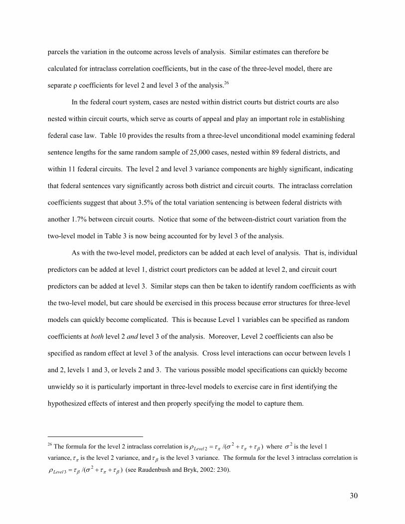
30

parcels the variation in the outcome across levels of analysis. Similar estimates can therefore be

calculated for intraclass correlation coefficients, but in the case of the three-level model, there are

separate ρ coefficients for level 2 and level 3 of the analysis.26

In the federal court system, cases are nested within district courts but district courts are also

nested within circuit courts, which serve as courts of appeal and play an important role in establishing

federal case law. Table 10 provides the results from a three-level unconditional model examining federal

sentence lengths for the same random sample of 25,000 cases, nested within 89 federal districts, and

within 11 federal circuits. The level 2 and level 3 variance components are highly significant, indicating

that federal sentences vary significantly across both district and circuit courts. The intraclass correlation

coefficients suggest that about 3.5% of the total variation sentencing is between federal districts with

another 1.7% between circuit courts. Notice that some of the between-district court variation from the

two-level model in Table 3 is now being accounted for by level 3 of the analysis.

As with the two-level model, predictors can be added at each level of analysis. That is, individual

predictors can be added at level 1, district court predictors can be added at level 2, and circuit court

predictors can be added at level 3. Similar steps can then be taken to identify random coefficients as with

the two-level model, but care should be exercised in this process because error structures for three-level

models can quickly become complicated. This is because Level 1 variables can be specified as random

coefficients at both level 2 and level 3 of the analysis. Moreover, Level 2 coefficients can also be

specified as random effect at level 3 of the analysis. Cross level interactions can occur between levels 1

and 2, levels 1 and 3, or levels 2 and 3. The various possible model specifications can quickly become

unwieldy so it is particularly important in three-level models to exercise care in first identifying the

hypothesized effects of interest and then properly specifying the model to capture them.

26

The formula for the level 2 intraclass correlation is )/(2

2 βππ ττστρ ++=Level where 2σ is the level 1

variance, πτ is the level 2 variance, and βτ is the level 3 variance. The formula for the level 3 intraclass correlation is

)/(2

3 βπβ ττστρ ++=Level (see Raudenbush and Bryk, 2002: 230).

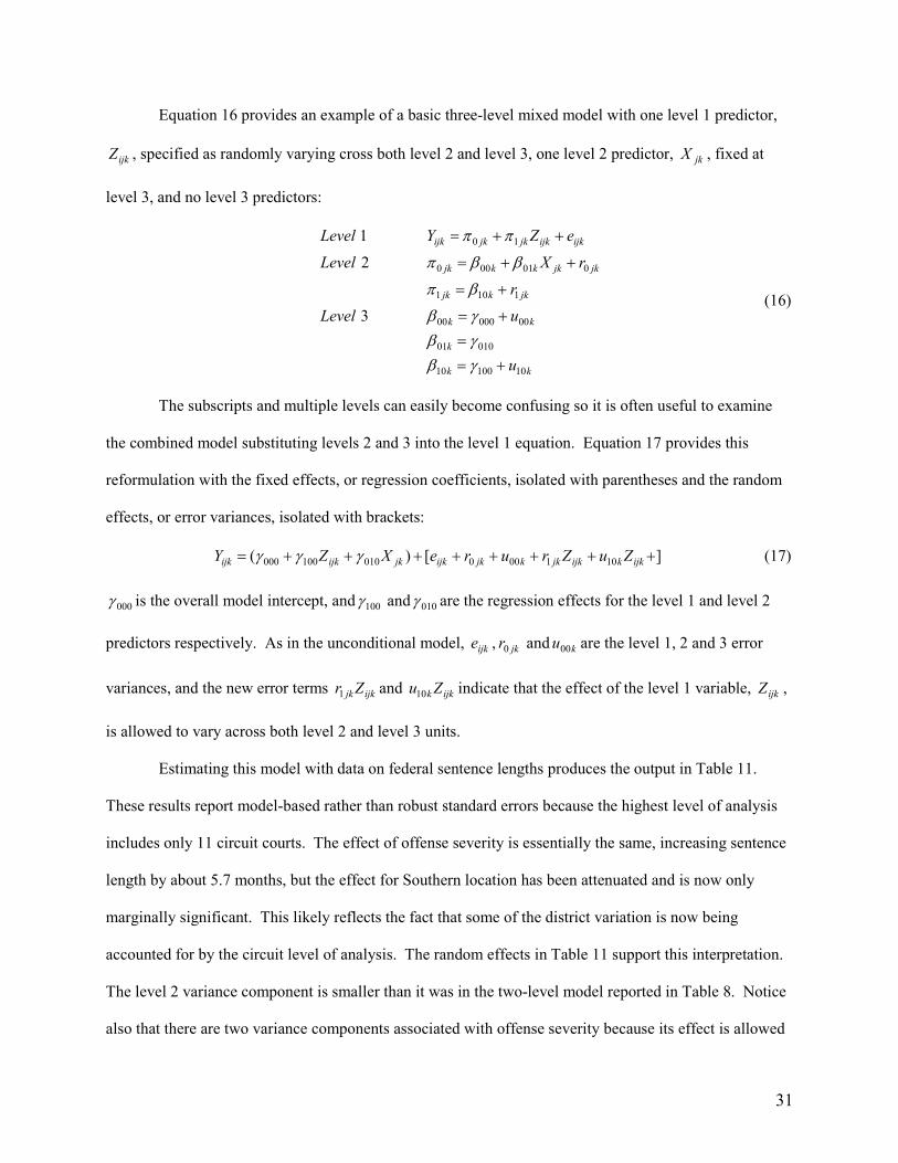
31

Equation 16 provides an example of a basic three-level mixed model with one level 1 predictor,

ijkZ , specified as randomly varying cross both level 2 and level 3, one level 2 predictor, jkX , fixed at

level 3, and no level 3 predictors:

kk

k

kk

jkkjk

jkjkkkjk

ijkijkjkjkijk

u

uLevel

r

rXLevel

eZYLevel

1010010

01001

0000000

1101

001000

10

3

2

1

+=

=

+=

+=

++=

++=

γβ

γβ

γβ

βπ

ββπ

ππ

(16)

The subscripts and multiple levels can easily become confusing so it is often useful to examine

the combined model substituting levels 2 and 3 into the level 1 equation. Equation 17 provides this

reformulation with the fixed effects, or regression coefficients, isolated with parentheses and the random

effects, or error variances, isolated with brackets:

][)( 101000010100000 ++++++++= ijkkijkjkkjkijkjkijkijk ZuZrureXZY γγγ (17)

000γ is the overall model intercept, and 100γ and 010γ are the regression effects for the level 1 and level 2

predictors respectively. As in the unconditional model, ijke , jkr0 and ku00 are the level 1, 2 and 3 error

variances, and the new error terms ijkjk Zr1 and ijkk Zu10 indicate that the effect of the level 1 variable, ijkZ ,

is allowed to vary across both level 2 and level 3 units.

Estimating this model with data on federal sentence lengths produces the output in Table 11.

These results report model-based rather than robust standard errors because the highest level of analysis

includes only 11 circuit courts. The effect of offense severity is essentially the same, increasing sentence

length by about 5.7 months, but the effect for Southern location has been attenuated and is now only

marginally significant. This likely reflects the fact that some of the district variation is now being

accounted for by the circuit level of analysis. The random effects in Table 11 support this interpretation.

The level 2 variance component is smaller than it was in the two-level model reported in Table 8. Notice

also that there are two variance components associated with offense severity because its effect is allowed

32

to vary both across district and circuit courts. The magnitude of these variance components indicates

there is more between-district than between-circuit variation in the effect of offense severity, but both are

highly significant. Although conceptually the three-level multilevel model represents a straightforward

extension of the two-level model, in practice care needs to be exercised to avoid exploding complexity

(for recent examples using 3 level models see Duncan et al., 2003; Johnson, 2006; Wright et al. 2007).

SUMMARY AND CONCLUSIONS

Multilevel models represent an increasingly popular analytical approach in the field of

criminology. According to a recent analysis by Gary Kleck (2006), between 5% and 6% of empirical

research papers in top criminology journals utilize multilevel modeling techniques; interestingly, though,

14% of these were published in the flagship journal for the field, Criminology. Given the omnipresence

of multilevel research questions in criminology, the use of multilevel analysis will continue to gain

prominence in the field. Because multilevel models provide a sophisticated approach for integrating

multiple levels of analysis, they represent an important opportunity to expand theoretical and empirical

discourse across a variety of criminological domains. Multilevel models have already been used to study

a rich diversity of topics, from examinations of self-control (Hay and Forrest, 2006; Doherty, 2006;

Wright and Beaver, 2005) and strain theory (Slocum et al. 2005) to life course perspectives (Horney et al.

1995; Sampson et al. 2006) and analyses of violent specialization (Osgood and Schreck, 2007) – from

crime victimization (Xie and McDowall, 2008; Wilcox et al. 2007), policing (Rosenfeld et al. 2007;

Warner, 2007) and punishment outcomes (Kleck et al. 2005; Bontrager et al. 2005; Johnson, 2005; 2006)

to post-release recidivism (Kubrin and Stewart, 2005; Chiricos et al. 2007; Mears et al. 2008) and

program evaluations (Gottfredson et al. 2007; Esbensen et al. 2001) – across a broad range of

criminological topic areas, multilevel models have proven to be invaluable tools.

Despite their many applications, though, the old adage that “A little bit of knowledge can be a

dangerous thing” applies directly to multilevel modeling. Modern software packages make estimating

multilevel models relatively simple, but the fully specified multilevel model often contains complicated

error structures that can easily be misspecified. Moreover, these complexities can sometimes result in

33

instability in parameter estimates. This is particularly the case for ecological predictors and for three-

level and generalized linear models. For instance, it is common for ecological predictors to have shared

variance (Land et al. 1990), so inclusion or elimination of one predictor can often affect the estimates for

other predictors in the model. It is therefore essential that the final model be carefully constructed from

the ground up, performing model diagnostics to test for misspecification, investigating problematic

collinearity and examining alternative models to ensure that the final estimates are robust to minor

alterations in model specification.

Although this chapter provides a basic overview of multilevel models, it is important to note that

it does not cover many of their advanced applications such as longitudinal data analysis, growth-curve

modeling, time series data, latent variable analysis, meta-analytical techniques or analysis of cross-

classified data. Beyond situations where individuals are influenced by social contexts, multilevel data

commonly characterizes these and many other criminological enterprises. As a discipline, we are just

beginning to incorporate the full range of applications for multilevel statistical models in the study of

crime and punishment. The goals of this chapter were simply to introduce the reader to the basic

multilevel model, to emphasize the ways in which it is similar to and different from the ordinary

regression model, to provide some brief examples of different types of multilevel models and to

demonstrate how they can be estimated within the context of jurisdictional variations in federal criminal

punishments across court contexts.

34

Figure 1: The Hierarchical Nature of Multiple Units of Analysis in Multilevel Models

Figure 2: The Nesting of Multilevel Data across Levels of Analysis

County

Court 1

Offender 1

Judge 1

Offender 3 Offender 2 Offender 4

Judge 2

Offender 6 Offender 5 Offender 7

Judge 3

Offender 9 Offender 8

Self -Control

Students

Classrooms

Schools

35

Figure 3: Variation in Trial Penalties across Federal Courts

36

Figure 4: Variation in Sentence Lengths across Federal Courts

Panel A: Pooled Data for Sample of 10 Districts

Panel B: Disaggregated Data for Sample of 10 Districts

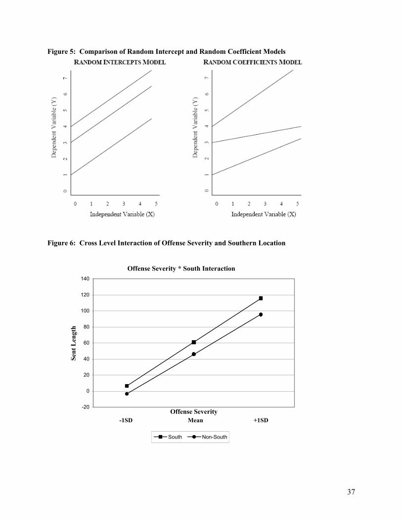
37

Figure 5: Comparison of Random Intercept and Random Coefficient Models

Figure 6: Cross Level Interaction of Offense Severity and Southern Location

Offense Severity * South Interaction

-20

0

20

40

60

80

100

120

140

Offense Severity

-1SD Mean +1SD

Sent Length

South Non-South

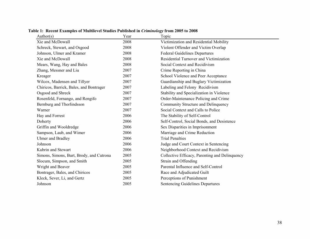
38

Table 1: Recent Examples of Multilevel Studies Published in Criminology from 2005 to 2008

Author(s) Year Topic

Xie and McDowall 2008 Victimization and Residential Mobility

Schreck, Stewart, and Osgood 2008 Violent Offender and Victim Overlap

Johnson, Ulmer and Kramer 2008 Federal Guidelines Departures

Xie and McDowall 2008 Residential Turnover and Victimization

Mears, Wang, Hay and Bales 2008 Social Context and Recidivism

Zhang, Messner and Liu 2007 Crime Reporting in China

Kreager 2007 School Violence and Peer Acceptance

Wilcox, Madensen and Tillyer 2007 Guardianship and Buglary Victimization

Chiricos, Barrick, Bales, and Bontrager 2007 Labeling and Felony Recidivism

Osgood and Shreck 2007 Stability and Specialization in Violence

Rosenfeld, Fornango, and Rengifo 2007 Order-Maintenance Policing and Crime

Bernburg and Thorlindsson 2007 Community Structure and Delinquency

Warner 2007 Social Context and Calls to Police

Hay and Forrest 2006 The Stability of Self-Control

Doherty 2006 Self-Control, Social Bonds, and Desistence

Griffin and Wooldredge 2006 Sex Disparities in Imprisonment

Sampson, Laub, and Wimer 2006 Marriage and Crime Reduction

Ulmer and Bradley 2006 Trial Penalties

Johnson 2006 Judge and Court Context in Sentencing

Kubrin and Stewart 2006 Neighborhood Context and Recidivism

Simons, Simons, Burt, Brody, and Cutrona 2005 Collective Efficacy, Parenting and Delinquency

Slocum, Simpson, and Smith 2005 Strain and Offending

Wright and Beaver 2005 Parental Influence and Self-Control

Bontrager, Bales, and Chiricos 2005 Race and Adjudicated Guilt

Kleck, Sever, Li, and Gertz 2005 Perceptions of Punishment

Johnson 2005 Sentencing Guidelines Departures

39

Table 2: Glossary of Multilevel Modeling Terminology

Terminology Definition

Aggregate VariableEcological variable created by aggregating the individual properties of lower level measures up to the group level of analysis.

Also sometimes referred to as "Derived" or "Analytical" variables.

Atomositic FallacyThe fallacy, also referred to as the Individualistic Fallacy, that results when faulty inferences for macro level group

relationships are drawn using micro-level individual data. See Ecological Fallacy

Compositional EffectsBetween group differences in outcomes that are attributable to differences in group composition, or in the different

individuals of which the groups are comprised.

Contextual AnalysisEarly analytical approach designed to investigate the effects of aggregate characteristics of the collective by including

aggregate variables along with individual variables in traditional regression models.

Contextual EffectsMacro-level influences exerted by aggregate variables above and beyond those attributable to compositional differences in

groups, but sometimes the term is used to refer to any group level effects.

Contextual Effects ModelStatistical model that include individual characteristics and the aggregates of the individual characteristics in the same model

in order to assess the influence of contextual effects on individual outcomes.

Cross-Level InteractionA statistical interaction between higher and lower order variables, usually attempting to explain variation in the effects of

lower level measures across higher level groupings.

Cross Classified ModelA multilevel statistical model for analyzing data that is cross-nested in two or more higher levels of analysis which are not

strictly hierarchical in structure. Also referred to as cross-nested models.

Ecological FallacyThe fallacy that results when faulty inferences for individual level relationships are made using group level data. (see

Atomistic Fallacy)

Ecological VariableA broad term for any higher order group level variable, including aggregate, structural and global measures. Sometimes

referred to as a Group Level, Macro Level, or Level 2 variables.

Empirical Bayes EstimatesEstimates for group level parameters that are optimally weighted to combine information from the individual group itself

with information from other similar groups in the data. See Conditional Shrinkage.

Fixed EffectsRegression coefficients (or intercepts) that are not allowed to vary randomly across higher level units. These are sometimes

referred to as fixed coefficients. See Random Effects/Coefficients.

Fixed Effects ModelsStatistical models in which all all effects or coefficients are fixed. Often this refers to the case where a dummy variable is

included for each higher level unit to remove between-group variation in the outcome.

40

Global VariableA group level variable that unlike Aggregate Variables has no individual analogue. Global (or Integral) Variables refer to

characteristics that are uniquely defined at the higher level of analysis.

Group Level VariableAn alternative name for ecological variables that measure any group level characteristic. Sometimes referred to as Level 2

Variables. See Individual Variable.

Hierarchical (Linear) ModelA multilevel model for analyzing data that is nested among two or more hierarchies. Hiearchical models technically assume

that data are strictly nested across levels of analysis, although this term may refer to multilevel models generally.

Individual Level VariableA variable that characterizes individual attributes or refers to individual level constructs. Sometimes referred to as Level 1

Variables. See Group Level Variable.

Intraclass CorrelationThe proportion of the total variance in the outcome that exists between groups or higher level units rather than within groups

or higher level units.

Mixed ModelA multilevel model containing both fixed and random coefficients. Some regression coefficients are allowed to vary

randomly across higher level units while other regression coefficients are specified as fixed coefficients.

Multilevel AnalysisAn analytical approach for simultaneously analyzing both individual and group level effects when data is measured at two or

more levels of analysis with lower level (micro) observations nested within higher level (macro) units.

Multilevel ModelA statistical model used in multilevel analysis for analyzing data that is measured at two or more levels of analysis, including

but not limited to hierarchical linear models, hiearchical nonlinear models, and cross-classified models.

Population Average EstimatesEstimates for nonlinear multilevel models that provide the marginal expectation of the outcome averaged across all random

effects rather than after controlling for random effects. See Unit-Specific Estimates

Random Coefficient ModelA multilvel statistical model in which the individual level intercept and regression coefficients are allowed to have randomly

varying effects across higher level units of analysis. See Random Intercept Model.

Random EffectsRegression coefficients (or intercepts) that are allowed to vary randomly across higher level units. These are sometimes

referred to as random intercepts or random coefficients. See Fixed Effects.

Random Intercept ModelA multilevel statistical model in which the individual level intercept is allowed to vary randomly across higher level units of

analysis, but the individual level coefficients are assumed to have constant effects. See Random Coefficient Model.

Unit Specific EstimatesEstimates for nonlinear multilevel models that are conditional on higher level random effects. Unit specific models provide

individual estimates controlling for rather than averaging across random effects. See Population Average Estimates

Variance ComponentsModel parameters (sometimes referred to as random effects) that explicitly capture both within-group and between-group

variability in outcomes. Each level of analysis in a multilevel model has its own variance component.

41

Table 3: Unconditional HLM Model of Federal Sentence Lengths

Sentence Length in Months

Fixed Effects b S.E. df p-value

Intercept (γ00) 52.5 1.8 88 0.00

Random Effects s2

S.D. df p-value ρ

Level 1 (r ij ) 4630.0 68.0

Level 2 (u oj ) 267.1 16.3 88 0.00 0.055

Deviance = 282173.7

Parameters = 2

N=25,000

Table 4: Random Intercept Model of Federal Sentence Lengths

Sentence Length in Months

Fixed Effects b S.E. df p-value

Intercept (γ00) 51.0 1.1 88 0.00

Severity (β1) 5.6 0.2 24998 0.00

Random Effects s2

S.D. df p-value

Level 1 (r ij ) 2228.7 47.2

Level 2 (u oj ) 93.2 9.7 88 0.00

Deviance = 263875.9

Parameters = 2

N=25,000

42

Table 5: Random Intercept Model of Federal Sentence Length

Sentence Length in Months

Fixed Effects b S.E. df p-value

Intercept (γ00) 50.9 1.0 87 0.00

South (γ01) 7.1 2.3 87 0.00

Severity (β1) 5.6 0.2 24997 0.00

Random Effects s2

S.D. df p-value

Level 1 (r ij ) 2228.7 47.2

Level 2 (u oj ) 82.4 9.1 87 0.00

Deviance = 263860.9

Parameters = 2

N=25,000

Table 6: Random Coefficient Model of Federal Sentence Length

Sentence Length in Months

Fixed Effects b S.E. df p-value

Intercept (γ00) 49.7 1.0 88 0.00

Severity (β1) 5.7 0.1 88 0.00

Random Effects s2

S.D. df p-value

Level 1 (r ij ) 2098.7 45.8

Level 2 (u oj ) 78.7 8.9 88 0.00

Severity (u 1j ) 1.4 1.2 88 0.00

Deviance = 262530.1

Parameters = 4

N=25,000

01γ

43

Table 7: Comparison of OLS, Random Intercept and Random Coefficient Models OLS REGRESSION RANDOM INTERCEPT RANDOM COEFFICIENT

Without Robust Errors Without Robust Errors Without Robust Errors

b S.E. b S.E. b S.E.

Intercept 47.9 0.30 Intercept 51.0 1.10 Intercept 49.7 1.02

Offense Severity 5.6 0.03 Offense Severity 5.6 .03 Offense Severity 5.7 .13

With Robust Errors With Robust Errors

b S.E. b S.E.

Intercept 51.0 1.06 Intercept 49.7 1.01

Offense Severity 5.6 .19 Offense Severity 5.7 .13

Deviance = 263875.9 Deviance = 262530.1

Parameters = 2 Parameters = 4

-65.36

12.10

89.56

167.03

244.49

SENTTOT2

1.00 13.25 25.50 37.75 50.00

XFOLSOR

2.00 14.00 26.00 38.00 50.00-64.91

6.60

78.10

149.61

221.11

XFOLSOR

SENTTOT2

2.00 14.00 26.00 38.00 50.00-53.61

12.33

78.28

144.23

210.17

XFOLSOR

SENTTOT2

Table 8: Random Coefficient Model with Level 2 Predictor of Federal Sentence Length

Sentence Length in Months

Fixed Effects b S.E. df p-value

Intercept (γ00) 49.6 1.0 87 0.00

South (γ01) 3.4 1.4 87 0.02

Severity (β1) 5.7 0.1 88 0.00

Random Effects s2

S.D. df p-value

Level 1 (r ij ) 2098.6 45.8

Level 2 (u oj ) 71.6 8.5 87 0.00

Severity (u 1j ) 1.5 1.2 88 0.00

44

Table 9: Cross-Level Interaction Model of Federal Sentence Length

Sentence Length in Months

Fixed Effects b S.E. df T-ratio p-value

Intercept (γ00) 49.6 1.0 87 49.14 0.00

South (γ01) 6.3 2.0 87 3.37 0.02

Severity (β1) 5.7 0.1 88 42.45 0.00

South*Severity (γ11) 0.6 0.3 87 2.07 0.04

Random Effects s2

S.D. df χ2

p-value

Level 1 (r ij ) 2098.6 45.8

Level 2 (u oj ) 70.2 8.4 87 1130.14 0.00

Severity (u 1j ) 1.4 1.2 88 1644.40 0.00

Deviance = 262519.3

Parameters = 4

N=25,000

Table 10: Multilevel Logistic Model of Federal Incarceration

Prison vs. No Prison (Unit-Specific Model with Robust Standard Errors)

Fixed Effects b S.E. df p-value Odds Ratio

Intercept (γ00) 2.80 0.08 87 0.00

South ( γ01) 0.07 0.11 87 0.53 1.07

Severity (β1) 0.26 0.01 88 0.00 1.29

Random Effects s2

S.D. df p-value

Level 2 (u 0j) .41 0.64 87 0.00

Severity (u 1j) .004 0.06 88 0.00

ijr

r

Table 11: Three-Level Unconditional Model of Federal Sentence Length

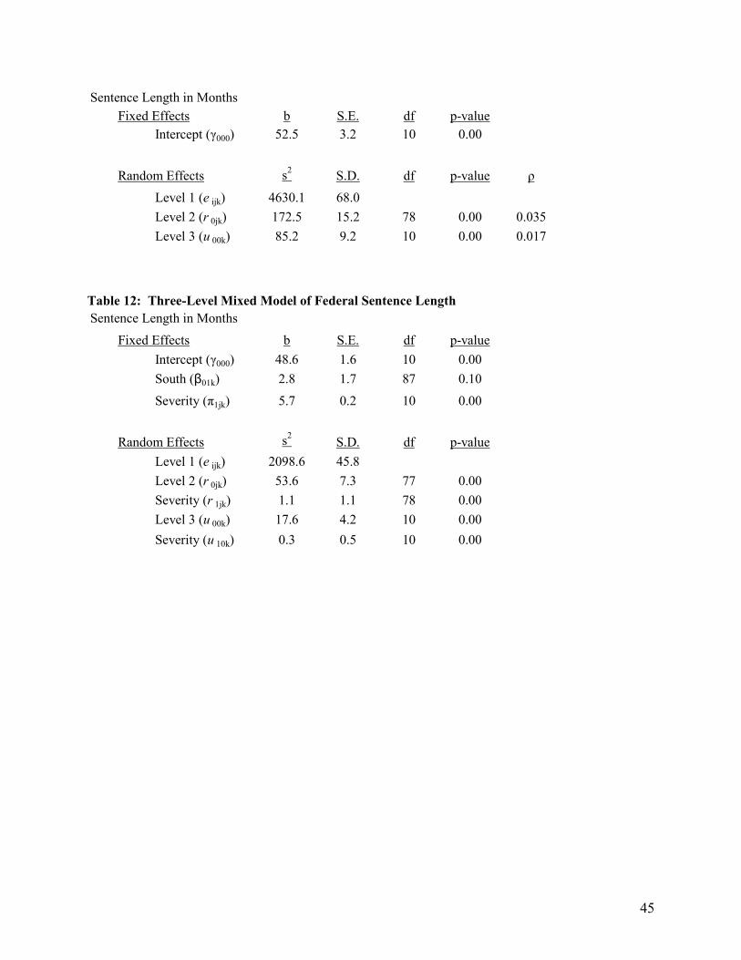
45

Sentence Length in Months

Fixed Effects b S.E. df p-value

Intercept (γ000) 52.5 3.2 10 0.00

Random Effects s2

S.D. df p-value ρ

Level 1 (e ijk) 4630.1 68.0

Level 2 (r 0jk) 172.5 15.2 78 0.00 0.035

Level 3 (u 00k) 85.2 9.2 10 0.00 0.017

Table 12: Three-Level Mixed Model of Federal Sentence Length

Sentence Length in Months

Fixed Effects b S.E. df p-value

Intercept (γ000) 48.6 1.6 10 0.00

South (β01k) 2.8 1.7 87 0.10

Severity (π1jk) 5.7 0.2 10 0.00

Random Effects s2

S.D. df p-value

Level 1 (e ijk) 2098.6 45.8

Level 2 (r 0jk) 53.6 7.3 77 0.00

Severity (r 1jk) 1.1 1.1 78 0.00

Level 3 (u 00k) 17.6 4.2 10 0.00

Severity (u 10k) 0.3 0.5 10 0.00

46

REFERENCES

Beaver, Kevin M. (2008). Nonshared Environmental influences on adolescent delinquent involvement

and adult criminal behavior. Criminology, 46(2), 341 – 369.

Bernburg, Jón Gunnar & Thorolfur Thorlindsson. (2007). Community structure and adolescent

delinquency in Iceland: A contextual analysis. Criminology, 45(2), 415 – 444.

Blalock, Hubert M. (1984). Contextual-effects models: Theoretical and methodological issues. Annual

Review of Sociology, 10, 353 – 372.

Blau, Peter M. (1960). Structural Effects. American Sociological Review, 25, 178 – 193.

Blumer, Hebert. (1958). Race prejudice as a sense of group position. Pacific Sociological Review,1, 3 – 7.

Bontrager, Stephanie, Bales, William & Ted Chiricos. (2005). Race, ethnicity, threat and the labeling of

convicted felons. Criminology, 43(3), 589 – 622.

Britt, Chester L. (2000). Social context and racial disparities in punishment decisions. Justice Quarterly,

17(4), 707 – 732.

Camp, Scott, Gaes, Gerald, Langan, Neal & William Saylor. (2003). The influence of prisons on inmate

misconduct: A multilevel investigation. Justice Quarterly, 20(3), 501 – 533.

Chiricos, Ted, Barrick, Kelle, Bales, William & Stephanie Bontrager. (2007). The labeling of convicted

felons and its consequences for recidivism. Criminology, 45(3), 547 – 581.

Diez Roux, A.V. (2002). A glossary for multilevel analysis. Journal of Epidemiology and Community

Health, 56, 588 – 594.

Doherty, Elaine Eggleston. (2006). Self-control, social bonds, and desistance: A test of life-course

interdependence. Criminology, 44(4), 807 – 833.

Duncan, Terry E., Duncan, Susan C., Okut, Hayrettin, Strycker, Lisa A. & Hollie Hix-Small. (2003). A

Multilevel Contextual Model of Neighborhood Collective Efficacy. American Journal of Community

Psychology, 32(3), 245 – 252.

Eitle, David, Lisa Stolzenberg & Stewart J D’Alessio. (2005). Police Organizational Factors, the Racial

Composition of the Police, and the Probability of Arrest. Justice Quarterly. 22(1): 30-57.

Emerson, Robert M. (1983). Holistic Effects in Social Control Decision-Making. Law & Society

Review. 17(3): 425-456.oHol

Esbensen Finn-Aage, D. Wayne Osgood, Terrance J. Taylor, Dana Peterson. (2001). How Great is

G.R.E.A.T.? Results from a Longitudinal Quasi-Experimental Design. Criminology & Public Policy

1(1): 87-118.

Firebaugh, G. (1978). A rule for inferring individual-level relationships from aggregate data. American

Sociological Review, 43, 557 – 572.

47

Gelman, Andrew & Jennifer Hill. (2007). Data Analysis Using Regression and Multilevel Hierarchical

Models. New York: Cambridge University Press.

Gillespie, Wayne. (2005). A Multilevel Model of Drug Abuse Inside Prison. The Prison Journal, 85(2),

223 – 246.

Goldstein, H. Yang, M. Omar, R., Turner R. & Thompson, S. (2000). Meta-analysis using multilevel

modelswith an application to the study of class size effects. Applied Statistics 49: 399-412.

Goldstein, Harvey. (1995). Multilevel Statistical Models. 2nd Ed. New York: John Wiley.

Gottfredson, Denise C., Cross, Amanda, and Soule, David A. (2007). Distinguishing Characteristics of

Effective and Ineffective After-School Programs to Prevent Delinquency and Victimization. Criminology

& Public Policy 6(2): 289-318.

Griffin, Marie L., & Gaylene S. Armstrong. (2003). The Effect of Local Life Circumstances on Female

Probationers’ Offending. Justice Quarterly. 20(2): 213-239.

Griffin, Timothy & John Wooldredge. (2006). Sex-based disparities in felony dispositions before versus

after sentencing reform in Ohio. Criminology, 44(4), 893 – 923.

Hay, Carter & Walter Forrest. (2006). The development of self-control: Examining self-control theory’s

stability thesis. Criminology, 44(4), 739 – 774.

Horney, Julie, Osgood, D. Wayne & Ineke Haen Marshall. (1995). Criminal Careers in the Short-Term:

Intra-Individual Variability in Crime and Its Relation to Local Life Circumstances. American

Sociological Review, 60(4), 655 – 673.

Hox, Joop. (2002). Multilevel Analysis: Techniques and Applications. Mahwah, NJ: Lawrence Erlbaum

Associates, Inc. Publishers.

Huebner, Beth M. (2003). Administrative determinants of inmate violence: A multilevel analysis. Journal

of Criminal Justice, 31(2), 107 – 117.

Johnson, Brian D. (2005). Contextual disparities in guidelines departures: Courtroom social contexts,

guidelines compliance, and extralegal disparities in criminal sentencing. Criminology, 43(3), 761 – 796.

Johnson, Brian D. (2006). The multilevel context of criminal sentencing: Integrating judge- and county-

level influences. Criminology, 44(2), 259 – 298.

Johnson, Brian D., Ulmer, Jeffrey T. & John H. Kramer. (2008). The social context of guidelines

circumvention: The case of federal district courts. Criminology, 46(3), 737 – 783.

Kleck, Gary, Tark, Jongyeon & Jon J. Bellows. (2006). What methods are most frequently used in

research in criminology and criminal justice? Journal of Criminal Justice, 36(2), 147 – 152.

Kleck Gary, Sever, Brion, Li, Spencer & Marc Gertz. (2005). The missing link in general deterrence

research. Criminology, 43(3), 623 – 660.

Kreager, Derek A. (2007). When it’s good to be “bad”: Violence and adolescent peer acceptance.

Criminology, 45(4), 893 – 923.

48

Kreft, Ita G. G. (1995). The Effects of Centering in Multilevel Analysis: Is the Public School the Loser or

the Winner? A New Analysis of an Old Question. Multilevel Modeling Newsletter 7: 5-8.

Kreft, Ita G. G., De Leeuw, Jan & Leona S. Aiken. (1995). The Effect of Different Forms of Centering in

Hierarchical Linear Models. Multivariate Behavioral Research, 30(1), 1 – 21.

Kreft, Ita G. G. & Jan De Leeuw. (1998). Introducing Multilevel Modeling. Thousand Oaks: Sage

Publications.

Kubrin, Charis E. & Eric A. Stewart. (2006). Predicting who reoffends: The neglected role of

neighborhood context in recidivism studies. Criminology, 44(1), 165 – 197.

Land, Kenneth C., Patricia L. McCall, and Lawrence E. Cohen. (1990). Structural Covariates of

Homicide Rates: Are There Any Invariances Across Time and Social Space? American Sociological

Review 95(4): 922-963.

Lauritsen, Janet L. & Robin J. Schaum. (2004). The social ecology of violence against women.

Criminology, 42(2), 323 – 357.

Lawton, Brian A. (2007). Levels of nonlethal force: An Examination of Individual, Situational and

Contextual Factors. Journal of Research in Crime and Delinquency, 44(2), 163 – 184.

Lee, Min Sik & Jeffery T. Ulmer. (2000). Fear of crime among Korean Americans in Chicago

communities. Criminology, 38(4), 1173 – 1206.

Liska, Allen E. (1990). The Significance of Aggregate Dependent Variables and Contextual Independent

Variables for Linking Macro and Micro Theories. Social Psych Quarterly, 53, 292 – 301.

Liska, Allen E. (1992). Social Threat and Social Control. Albany: SUNY Press.

Longford, N.T. (1989). To center or not to center. Multilevel Modelling Newsletter, 1(2), 7 - 11.

Luke, Douglas A. (2004). Multilevel Modeling. Thousand Oaks: Sage Publications.

Mears, Daniel P., Wang, Xia, Hay, Carter & William D. Bales. Social ecology and recidivism:

Implications for prisoner reentry. Criminology, 46(2), 301 – 340.

Miethe, Terance D., & David McDowall. (1993). Contextual Effects in Models of Criminal

Victimization. Social Forces. 71(3): 741-759.

Mill, John S. (1843). A System of Logic, Ratiocinative, and Inductive. London: Longmans, Green,

Reader, and Dyer. [8th ed., 1872] or “Harrison & Co.” for 1st ed.

Nieuwbeerta, Paul, McCall, Patricia L., Elffers, Henk & Karin Wittebrood. (2008). Neighborhood

Characteristics and Individual Homicide Risks: Effects of Social Cohesion, Confidence, in the Police, and

Socioeconomic Disadvantage. Homicide Studies, 12(1), 90 – 116.

Osgood, D. Wayne, & Anderson, Amy L. (2004). Unstructured socializing and rates of delinquency.

Criminology, 42(3), 519 – 550.

49

Osgood, D. Wayne & Christopher J. Schreck. (2007). A new method for studying the extent, stability, and

predictors of individual specialization in violence. Criminology, 45(2), 273 – 312.

Paccagnella, Omar. (2006). Centering or Not Centering in Multilevel Models? The Role of the Group

Mean and the Assessment of Group Effects. Evaluation Review 30(1): 66-85.

Pare, Paul-Philippe, Felson, Richard B. & Marc Ouimet. (2007). Community Variation in Crime

Clearance Multilevel Analysis with Comments on Assessing Police Performance. Journal of Quantitative

Criminology, 23(3), 243 – 258.

Rankin, Bruce H., and James M. Quane. (2002). Social Contexts and Urban Adolescent Outcomes: The

Interrelated Effects of Neighborhoods, Families, and Peers on African-American Youth. Social Problems

49(1): 79-100.

Raudenbush, Stephen W. (1984). Magnitude of Teacher Expectancy Effects on Pupil IQ as a Function of

Credibility of Expectancy Induction: A Synthesis of Findings from 18 Experiments. Journal of

Educational Psychology, 76(1), 85 – 97.

Raudenbush, Stephen W. (1989). “Centering” predictors in multilevel analysis. Choices and

consequences. Multilevel Modeling Newsletter 1:10-12.

Raudenbush, Stephen W. & Anthony S. Bryk. (2002). Hierarchical Linear Models: Applications and Data

Analysis Methods, 2nd Edition. SAGE Publications Inc.

Robinson, W.S. (1950). Ecological Correlations and the Behavior of Individuals. American Sociological

Review 15: 351–357

Rosenfeld, Richard, Baumer, Eric & Steven Messner. (2007). Social Trust, Firearm Prevalence, and

Homicide. Annals of Epidemiology, 17(2), 119 – 125.

Rosenfeld, Richard, Fornango, Robert & Andres F. Rengifo. (2007). The impact of order-maintenance

policing in New York City homicide and robbery rates: 1988 – 2001. Criminology, 45(2), 355 – 384.

Sampson, Robert J., Laub, John H. & Christopher Wimer. (2006). Does marriage reduce crime? A

counterfactual approach to within-individual causal effects. Criminology, 44(3), 465 – 508.

Schreck, Christopher J., Stewart, Eric A. & D. Wayne Osgood. (2008). A reappraisal of the overlap of

violent offenders and victims. Criminology, 46(4), 871 – 906).

Simons, Ronald L., Simons, Leslie Gordon, Burt, Callie Harbin, Brody, Gene H. & Carolyn Cutrona.

(2005). Collective efficacy, authoritative parenting and delinquency: A longitudinal test of a model

integrating community- and felony-level processes. Criminology, 43(4), 989 – 1029.

Slocum, Lee Ann, Simpson, Sally & Douglas A. Smith. (2005). Strained lives and crime: Examining

intra-individual variation in strain and offending in a sample of incarcerated women. Criminology, 43(4),

1067 – 110.

Smith, Douglas. (1986). The Neighborhood Context of Police Behavior. Crime and Justice: A Review of

Research 8: 313-341.

50

Snidjers, Tom & Roel Bosker. (1999). Multilevel Models: An Introduction to Basic and Advanced

Multilevel Modeling. Thousand Oaks: Sage Publications.

Stewart, Eric A. (2003). School social bonds, school climate, and school misbehavior: A multilevel

analysis. Justice Quarterly, 20(3), 575 – 604.

Sun, Ivan Y., Payne, Brian K. & Yuning Wu. (2008). The impact of situational factors, officer

characteristics, and neighborhood context on police behavior: A multilevel analysis. Journal of Criminal

Justice, 36(1), 22 – 32.

Taylor, Jeanette, Malone, Steve, Iacono, William G. & Matt McGue. (2002). Development of Substance

Dependence in Two Delinquency Subgroups and Nondelinquents From a Male Twin Sample. Journal of

the American Academy of Child & Adolescent Psychiatry, 41(4), 386 – 393.

Terrill, William & Michael D. Reisig. (2003). Neighborhood Context and Police Use of Force. Journal of

Research in Crime and Delinquency, 40(3), 291 – 321.

Ulmer, Jeffrey T. & Mindy S. Bradley. (2006). Variation in trial penalties among serious violent offenses.

Criminology, 44(3), 631 – 670.

Ulmer, Jeffery T. & Brian D. Johnson. (2004). Sentencing in context: A multilevel analysis. Criminology,

42(1), 137 – 178.

Warner, Barbara D. (2007). Directly intervene or call the authorities? A study of forms of neighborhood

social control within a social disorganization framework. Criminology, 45(1), 99 – 129.

Wilcox, Pamela, Madensen, Tamara D., & Marie S. Tillyer (2007). Guardianship in context: Implications

for burglary victimization risk and prevention. Criminology, 45(4), 771 – 803.

Wooldredge, John, Griffin, Timothy & Travis Pratt. (2001). Considering hierarchical models for research

on inmate behavior: Predicting misconduct with multilevel data. Justice Quarterly, 18(1), 203 – 231.

Wooldredge, John. (2007). Neighborhood Effects on Felony Sentencing. Journal of Research in Crime

and Delinquency, 44(2), 238 – 263.

Wright, John P. & Kevin M. Beaver. (2005). Do parents matter in creating self-control in their children?

A genetically informed test of Gottfredson and Hirschi’s theory of low self-control. Criminology, 43(4),

1169 – 1202.

Wright, John P., Beaver, Kevin M., Delisi, Matt & Michael Vaughn. (2008). Evidence of Negligible

Parenting Influence on Self-Control, Delinquent Peers, and Delinquency in a Sample of Twins. Justice

Quarterly, 25(3), 544 – 569.

Wright, Douglas A., Bobashev, Georgiy & Ralph Folsom. (2007). Understanding the Relative Influence

of Neighborhood, Family, and Youth on Adolescent Drug Use. Substance Use & Misuse, 42, 2159 –

2171.

Wyant, Brian R. (2008). Multilevel Impacts of Perceived Incivilities and Perceptions of Crime Risk on

Fear of Crime: Isolating Endogenous Impacts. Journal of Research in Crime and Delinquency, 45(1), 39 –

64.

51

Xie, Min & David McDowall. (2008). Escaping Crime: The effects of direct and indirect victimization

on moving. Criminology 46(4): 809-840.

Xie, Min & David McDowall. (2008). The effects of residential turnover on household victimization.

Criminology, 46(3), 539 – 575.

Zhang, Lening, Messner, Steven F. & Jianhong Liu. (2007). An exploration of the determinants of

reporting crime to the police in the city of Tianjin, China. Criminology, 45(4), 959 – 984.