nag fortran library routine document e04ugf … fortran library routine document e04ugf=e04uga note:...

NAG Fortran Library Routine Document

E04UGF=E04UGA

Note: before using this routine, please read the Users’ Note for your implementation to check the interpretation of bold italicised terms andother implementation-dependent details.

Note: this routine uses optional parameters to define choices in the problem specification and in the details of

the algorithm. If you wish to use default settings for all of the optional parameters, you need only read

Section 1 to Section 9 of this document. Refer to the additional Section 10, Section 11 and Section 12 for a

detailed description of the algorithm, the specification of the optional parameters and a description of the

monitoring information produced by the routine.

1 Purpose

E04UGF=E04UGA solves sparse nonlinear programming problems.

E04UGA is a version of E04UGF that has additional parameters in order to make it safe for use inmultithreaded applications (see Section 5 below). The initialisation routine E04WBF must have beencalled prior to calling E04UGA.

2 Specifications

2.1 Specification for E04UGF

SUBROUTINE E04UGF(CONFUN, OBJFUN, N, M, NCNLN, NONLN, NJNLN, IOBJ, NNZ,1 A, HA, KA, BL, BU, START, NNAME, NAMES, NS, XS,2 ISTATE, CLAMDA, MINIZ, MINZ, NINF, SINF, OBJ, IZ,3 LENIZ, Z, LENZ, IUSER, USER, IFAIL)

INTEGER N, M, NCNLN, NONLN, NJNLN, IOBJ, NNZ, HA(NNZ),1 KA(N+1), NNAME, NS, ISTATE(N+M), MINIZ, MINZ, NINF,2 IZ(LENIZ), LENIZ, LENZ, IUSER(*), IFAILreal A(NNZ), BL(N+M), BU(N+M), XS(N+M), CLAMDA(N+M), SINF,

1 OBJ, Z(LENZ), USER(*)CHARACTER*1 STARTCHARACTER*8 NAMES(NNAME)EXTERNAL CONFUN, OBJFUN

2.2 Specification for E04UGA

SUBROUTINE E04UGA(CONFUN, OBJFUN, N, M, NCNLN, NONLN, NJNLN, IOBJ, NNZ,1 A, HA, KA, BL, BU, START, NNAME, NAMES, NS, XS,2 ISTATE, CLAMDA, MINIZ, MINZ, NINF, SINF, OBJ, IZ,3 LENIZ, Z, LENZ, IUSER, USER, LWSAV, IWSAV, RWSAV,4 IFAIL)

INTEGER N, M, NCNLN, NONLN, NJNLN, IOBJ, NNZ, HA(NNZ),1 KA(N+1), NNAME, NS, ISTATE(N+M), MINIZ, MINZ, NINF,2 IZ(LENIZ), LENIZ, LENZ, IUSER(*), IWSAV(550), IFAILreal A(NNZ), BL(N+M), BU(N+M), XS(N+M), CLAMDA(N+M), SINF,

1 OBJ, Z(LENZ), USER(*), RWSAV(550)LOGICAL LWSAV(20)CHARACTER*1 STARTCHARACTER*8 NAMES(NNAME)EXTERNAL CONFUN, OBJFUN

Before calling E04UGA, or either of the option setting routines E04UHA or E04UJA, routine E04WBFmust be called. The specification for E04WBF is:

SUBROUTINE E04WBF(RNAME, CWSAV, LCWSAV, LWSAV, LLWSAV, IWSAV, LIWSAV,1 RWSAV, LRWSAV, IFAIL)

INTEGER LCWSAV, LLWSAV, IWSAV(LIWSAV), LIWSAV, LRWSAV, IFAILreal RWSAV(LRWSAV)LOGICAL LWSAV(LLWSAV)CHARACTER*6 RNAMECHARACTER*80 CWSAV(LCWSAV)

E04 – Minimizing or Maximizing a Function E04UGF=E04UGA

[NP3546/20A] E04UGF=E04UGA.1

E04WBF should be called with RNAME ¼ ’E04UGA’. LCWSAV, LLWSAV, LIWSAV and LRWSAV, thedeclared lengths of CWSAV, LWSAV, IWSAV and RWSAV respectively, must satisfy:

LCWSAV � 1

LLWSAV � 20

LIWSAV � 550

LRWSAV � 550

The contents of the arrays CWSAV, LWSAV, IWSAV and RWSAV must not be altered between callingroutines E04WBF and E04UGA, E04UHA or E04UJA.

3 Description

E04UGF=E04UGA is designed to solve a class of nonlinear programming problems that are assumed to bestated in the following general form:

minimizex2Rn

fðxÞ subject to l �x

F ðxÞGx

8<:

9=; � u; ð1Þ

where x ¼ ðx1; x2; . . . ; xnÞT is a set of variables, fðxÞ is a smooth scalar objective function, l and u areconstant lower and upper bounds, F ðxÞ is a vector of smooth nonlinear constraint functions fFiðxÞg and Gis a sparse matrix.

The constraints involving F and Gx are called the general constraints. Note that upper and lower boundsare specified for all variables and constraints. This form allows full generality in specifying various typesof constraint. In particular, the jth constraint can be defined as an equality by setting lj ¼ uj. If certain

bounds are not present, the associated elements of l or u can be set to special values that will be treated as�1 or þ1. (See the description of the optional parameter Infinite Bound Size.)

E04UGF=E04UGA converts the upper and lower bounds on the m elements of F and Gx to equalities by

introducing a set of slack variables s, where s ¼ ðs1; s2; . . . ; smÞT . For example, the linear constraint5 � 2x1 þ 3x2 � þ1 is replaced by 2x1 þ 3x2 � s1 ¼ 0, together with the bounded slack 5 � s1 � þ1.The problem defined by (1) can therefore be re-written in the following equivalent form:

minimizex2Rn;s2Rm

fðxÞ subject to Gxf g � s ¼ 0; l � xs

� �� u: ð2Þ

Since the slack variables s are subject to the same upper and lower bounds as the elements of F and Gx,the bounds on F and Gx can simply be thought of as bounds on the combined vector ðx; sÞ. The elementsof x and s are partitioned into basic, nonbasic and superbasic variables defined as follows:

A basic variable (xj say) is the jth variable associated with the jth column of the basis matrix B.

A nonbasic variable is a variable that is temporarily fixed at its current value (usually its upper orlower bound).

A superbasic variable is a nonbasic variable which is not at one of its bounds that is free to move inany desired direction (namely one that will improve the value of the objective function or reduce thesum of infeasibilities).

For example, in the simplex method (see Gill et al. (1981)) the elements of x can be partitioned at eachvertex into a set of m basic variables (all non-negative) and a set of ðn�mÞ nonbasic variables (all zero).This is equivalent to partitioning the columns of the constraint matrix as ðB j NÞ, where B contains the mcolumns that correspond to the basic variables and N contains the ðn�mÞ columns that correspond to thenonbasic variables. Note that B is square and non-singular.

The optional parameter Maximize may be used to specify an alternative problem in which fðxÞ ismaximized. If the objective function is nonlinear and all the constraints are linear, F is absent and theproblem is said to be linearly constrained. In general, the objective and constraint functions are structuredin the sense that they are formed from sums of linear and nonlinear functions. This structure can beexploited by the routine during the solution process as follows.

E04UGF=E04UGA NAG Fortran Library Manual

E04UGF=E04UGA.2 [NP3546/20A]

Consider the following nonlinear optimization problem with four variables (u; v; z; w):

minimizeu;v;z;w

ðuþ vþ zÞ2 þ 3z þ 5w

subject to the constraints

u2 þ v2 þ z ¼ 2

u4 þ v4 þ w ¼ 4

2uþ 4v � 0

and to the bounds

z � 0

w � 0:

This problem has several characteristics that can be exploited by the routine:

The objective function is nonlinear. It is the sum of a nonlinear function of the variables (u; v; z)and a linear function of the variables (z; w).

The first two constraints are nonlinear. The third is linear.

Each nonlinear constraint function is the sum of a nonlinear function of the variables (u; v) and alinear function of the variables (z; w).

The nonlinear terms are defined by the user-supplied subroutines OBJFUN and CONFUN (see Section 5),which involve only the appropriate subset of variables.

For the objective, we define the function fðu; v; zÞ ¼ ðuþ vþ zÞ2 to include only the nonlinear part of theobjective. The three variables (u; v; z) associated with this function are known as the nonlinear objectivevariables. The number of them is given by NONLN (see Section 5) and they are the only variablesneeded in OBJFUN. The linear part 3zþ 5w of the objective is stored in row IOBJ (see Section 5) of the(constraint) Jacobian matrix A (see below).

Thus, if x0 and y0 denote the nonlinear and linear objective variables, respectively, the objective may be re-written in the form

fðx0Þ þ cTx0 þ dTy0;

where fðx0Þ is the nonlinear part of the objective and c and d are constant vectors that form a row of A.In this example, x0 ¼ (u; v; z) and y0 ¼ w.

Similarly for the constraints, we define a vector function F ðu; vÞ to include just the nonlinear terms. In

this example, F1ðu; vÞ ¼ u2 þ v2 and F2ðu; vÞ ¼ u4 þ v4, where the two variables (u; v) are known as thenonlinear Jacobian variables. The number of them is given by NJNLN (see Section 5) and they are the

only variables needed in CONFUN. Thus, if x00 and y00 denote the nonlinear and linear Jacobian variables,respectively, the constraint functions and the linear part of the objective have the form

F ðx00Þ þA2y00

A3x00 þA4y

00

� �; ð3Þ

where x00 ¼ ðu; vÞ and y00 ¼ ðz; wÞ in this example. This ensures that the Jacobian is of the form

A ¼ Jðx00Þ A2

A3 A4

� �;

where Jðx00Þ ¼ @F ðx00Þ@x

. Note that Jðx00Þ always appears in the top left-hand corner of A.

The inequalities l1 � F ðx00Þ þA2y00 � u1 and l2 � A3x

00 þA4y00 � u2 implied by the constraint functions

in (3) are known as the nonlinear and linear constraints, respectively. The nonlinear constraint vector

F ðx00Þ in (3) and (optionally) its partial derivative matrix Jðx00Þ are set in CONFUN. The matrices A2, A3

and A4 contain any (constant) linear terms. Along with the sparsity pattern of Jðx00Þ they are stored in thearrays A, HA and KA (see Section 5).


[NP3546/20A] E04UGF=E04UGA.3

In general, the vectors x0 and x00 have different dimensions, but they always overlap, in the sense that theshorter vector is always the beginning of the other. In the above example, the nonlinear Jacobian variablesðu; vÞ are an ordered subset of the nonlinear objective variables ðu; v; zÞ. In other cases it could be the

other way round (whichever is the most convenient), but the first way keeps Jðx00Þ as small as possible.

Note that the nonlinear objective function fðx0Þ may involve either a subset or superset of the variables

appearing in the nonlinear constraint functions F ðx00Þ. Thus, NONLN � NJNLN (or vice-versa).Sometimes the objective and constraints really involve disjoint sets of nonlinear variables. In such cases

the variables should be ordered so that NONLN > NJNLN and x0 ¼ ðx00; x000Þ, where the objective is

nonlinear in just the last vector x000. The first NJNLN elements of the gradient array OBJGRD should alsobe set to zero in OBJFUN. This is illustrated in Section 9.

If all elements of the constraint Jacobian are known (i.e., the optional parameter Derivative Level ¼ 2 or3), any constant elements may be assigned their correct values in A, HA and KA. The correspondingelements of the constraint Jacobian array FJAC need not be reset in CONFUN. This includes values thatare identically zero as constraint Jacobian elements are assumed to be zero unless specified otherwise. Itmust be emphasized that, if Derivative Level ¼ 0 or 1, unassigned elements of FJAC are not treated asconstant; they are estimated by finite differences, at non-trivial expense.

If there are no nonlinear constraints in (1) and fðxÞ is linear or quadratic, then it may be more efficient touse E04NKF=E04NKA to solve the resulting linear or quadratic programming problem, or one ofE04MFF=E04MFA, E04NCF=E04NCA or E04NFF=E04NFA if G is a dense matrix. If the problem isdense and does have nonlinear constraints then one of E04UCF=E04UCA, E04UFF=E04UFA orE04USF=E04USA (as appropriate) should be used instead.

You must supply an initial estimate of the solution to (1), together with versions of OBJFUN and

CONFUN that define fðx0Þ and F ðx00Þ, respectively, and as many first partial derivatives as possible. Notethat if there are any nonlinear constraints, then the first call to CONFUN will precede the first call toOBJFUN.

E04UGF=E04UGA is based on the SNOPT package described in Gill et al. (1997), which in turn utilizesroutines from the MINOS package (see Murtagh and Saunders (1995)). It incorporates a sequentialquadratic programming (SQP) method that obtains search directions from a sequence of quadraticprogramming (QP) subproblems. Each QP subproblem minimizes a quadratic model of a certainLagrangian function subject to a linearization of the constraints. An augmented Lagrangian merit functionis reduced along each search direction to ensure convergence from any starting point. Further details canbe found in Section 10.

Throughout this document the symbol � is used to represent the machine precision (see X02AJF).

4 References

Gill P E, Murray W and Saunders M A (1997) SNOPT: An SQP Algorithm for Large-scale ConstrainedOptimization Numerical Analysis Report 97–2 Department of Mathematics, University of California, SanDiego

Gill P E, Murray W, Saunders M A and Wright M H (1992) Some theoretical properties of an augmentedLagrangian merit function Advances in Optimization and Parallel Computing (ed P M Pardalos) 101–128North Holland

Gill P E, Murray W, Saunders M A and Wright M H (1986) User’s guide for NPSOL (Version 4.0) ReportSOL 86-2 Department of Operations Research, Stanford University

Gill P E, Murray W, Saunders M A and Wright M H (1989) A practical anti-cycling procedure for linearlyconstrained optimization Math. Programming 45 437–474

Gill P E, Murray W and Wright M H (1981) Practical Optimization Academic Press

Conn A R (1973) Constrained optimization using a nondifferentiable penalty function SIAM J. Numer.Anal. 10 760–779

Eldersveld S K (1991) Large-scale sequential quadratic programming algorithms PhD Thesis Departmentof Operations Research, Stanford University, Stanford


E04UGF=E04UGA.4 [NP3546/20A]

Fletcher R (1984) An l1 penalty method for nonlinear constraints Numerical Optimization 1984 (ed P TBoggs, R H Byrd and R B Schnabel) 26–40 SIAM Philadelphia

Fourer R (1982) Solving staircase linear programs by the simplex method Math. Programming 23 274–313

Hock W and Schittkowski K (1981) Test Examples for Nonlinear Programming Codes. Lecture Notes inEconomics and Mathematical Systems 187 Springer-Verlag

Murtagh B A and Saunders M A (1995) MINOS 5.4 User’s Guide Report SOL 83-20R Department ofOperations Research, Stanford University

Ortega J M and Rheinboldt W C (1970) Iterative Solution of Nonlinear Equations in Several VariablesAcademic Press

Powell M J D (1974) Introduction to constrained optimization Numerical Methods for ConstrainedOptimization (ed P E Gill and W Murray) 1–28 Academic Press

5 Parameters

Note: all optional parameters are described in detail in Section 11.2.

1: CONFUN – SUBROUTINE, supplied by the user. External Procedure

CONFUN must calculate the vector F ðxÞ of nonlinear constraint functions and (optionally) its

Jacobian ¼ @F

@x

� �for a specified n00

1 (� n) element vector x. If there are no nonlinear constraints

(i.e., NCNLN ¼ 0), CONFUN will never be called by E04UGF=E04UGA and CONFUN may bethe dummy routine E04UGM. (E04UGM is included in the NAG Fortran Library and so need notbe supplied by the user. Its name may be implementation-dependent: see the Users’ Note for yourimplementation for details.) If there are nonlinear constraints, the first call to CONFUN will occurbefore the first call to OBJFUN.

Its specification is:

SUBROUTINE CONFUN(MODE, NCNLN, NJNLN, NNZJAC, X, F, FJAC, NSTATE,1 IUSER, USER)

INTEGER MODE, NCNLN, NJNLN, NNZJAC, NSTATE, IUSER(*)real X(NJNLN), F(NCNLN), FJAC(NNZJAC), USER(*)

1: MODE – INTEGER Input/Output

On entry: MODE indicates which values must be assigned during each call of CONFUN.Only the following values need be assigned:

if MODE ¼ 0, F;

if MODE ¼ 1, all available elements of FJAC;

if MODE ¼ 2, F and all available elements of FJAC.

On exit: MODE may be set to a negative value by the user as follows:

if MODE � �2, the solution to the current problem is terminated and in this caseE04UGF=E04UGA will terminate with IFAIL set to MODE;

if MODE ¼ �1, the nonlinear constraint functions cannot be calculated at thecurrent x. E04UGF=E04UGA will then terminate with IFAIL set to �1 unless thisoccurs during the linesearch; in this case, the linesearch will shorten the step and tryagain.

2: NCNLN – INTEGER Input

On entry: nN , the number of nonlinear constraints. These must be the first NCNLNconstraints in the problem.


[NP3546/20A] E04UGF=E04UGA.5

3: NJNLN – INTEGER Input

On entry: n001, the number of nonlinear variables. These must be the first NJNLN variables

in the problem.

4: NNZJAC – INTEGER Input

On entry: the number of non-zero elements in the constraint Jacobian. Note that NNZJACwill usually be less than NCNLN � NJNLN.

5: X(NJNLN) – real array Input

On entry: x, the vector of nonlinear Jacobian variables at which the nonlinear constraintfunctions and/or the available elements of the constraint Jacobian are to be evaluated.

6: F(NCNLN) – real array Output

On exit: if MODE ¼ 0 or 2, FðiÞ must contain the value of the ith nonlinear constraintfunction at x.

7: FJAC(NNZJAC) – real array Output

On exit: if MODE ¼ 1 or 2, FJAC must return the available elements of the constraintJacobian evaluated at x. These elements must be stored in exactly the same positions asimplied by the definitions of the arrays A, HA and KA described below. If DerivativeLevel ¼ 2 or 3 (default value ¼ 3), the value of any constant Jacobian element not definedby CONFUN will be obtained directly from A. Note that the routine does not performany internal checks for consistency (except indirectly via the optional parameter VerifyLevel), so great care is essential.

8: NSTATE – INTEGER Input

On entry: if NSTATE ¼ 1, then E04UGF=E04UGA is calling CONFUN for the first time.This parameter setting allows the user to save computation time if certain data must beread or calculated only once. If NSTATE � 2, then E04UGF=E04UGA is callingCONFUN for the last time. This parameter setting allows the user to perform someadditional computation on the final solution. In general, the last call to CONFUN is madewith NSTATE ¼ 2þ IFAIL (see Section 6). Otherwise, NSTATE ¼ 0.

9: IUSER(*) – INTEGER array User Workspace10: USER(*) – real array User Workspace

CONFUN is called from E04UGF=E04UGA with the parameters IUSER and USER assupplied to E04UGF=E04UGA. The user is free to use the arrays IUSER and USER tosupply information to CONFUN as an alternative to using COMMON.

CONFUN must be declared as EXTERNAL in the (sub)program from which E04UGF=E04UGA iscalled. Parameters denoted as Input must not be changed by this procedure.

CONFUN must be declared as EXTERNAL in the (sub)program from which E04UGF=E04UGA iscalled and should be tested separately before being used in conjunction with E04UGF=E04UGA.Parameters denoted as Input must not be changed by this procedure.

2: OBJFUN – SUBROUTINE, supplied by the user. External Procedure

OBJFUN must calculate the nonlinear part of the objective function fðxÞ and (optionally) its

gradient ¼ @f

@x

� �for a specified n0

1 (� n) element vector x. If there are no nonlinear objective

variables (i.e., NONLN ¼ 0), OBJFUN will never be called by E04UGF=E04UGA and OBJFUNmay be the dummy routine E04UGN. (E04UGN is included in the NAG Fortran Library and soneed not be supplied by the user. Its name may be implementation-dependent: see the Users’ Notefor your implementation for details.)


E04UGF=E04UGA.6 [NP3546/20A]

Its specification is:

SUBROUTINE OBJFUN(MODE, NONLN, X, OBJF, OBJGRD, NSTATE, IUSER, USER)

INTEGER MODE, NONLN, NSTATE, IUSER(*)real X(NONLN), OBJF, OBJGRD(NONLN), USER(*)

1: MODE – INTEGER Input/Output

On entry: MODE indicates which values must be assigned during each call of OBJFUN.Only the following values need be assigned:

if MODE ¼ 0, OBJF;

if MODE ¼ 1, all available elements of OBJGRD;

if MODE ¼ 2, OBJF and all available elements of OBJGRD.

On exit: MODE may be set to a negative value by the user as follows:

if MODE � �2, the solution to the current problem is terminated and in this caseE04UGF=E04UGA will terminate with IFAIL set to MODE;

if MODE ¼ �1, the nonlinear part of the objective function cannot be calculated atthe current x. E04UGF=E04UGA will then terminate with IFAIL set to �1 unlessthis occurs during the linesearch; in this case, the linesearch will shorten the stepand try again.

2: NONLN – INTEGER Input

On entry: n01, the number of nonlinear objective variables. These must be the first

NONLN variables in the problem.

3: X(NONLN) – real array Input

On entry: x, the vector of nonlinear variables at which the nonlinear part of the objectivefunction and/or all available elements of its gradient are to be evaluated.

4: OBJF – real Output

On exit: if MODE ¼ 0 or 2, OBJF must be set to the value of the objective function at x.

5: OBJGRD(NONLN) – real array Output

On exit: if MODE ¼ 1 or 2, OBJGRD must return the available elements of the gradientevaluated at x.

6: NSTATE – INTEGER Input

On entry: if NSTATE ¼ 1 then E04UGF=E04UGA is calling OBJFUN for the first time.This parameter setting allows the user to save computation time if certain data must beread or calculated only once. If NSTATE � 2 then E04UGF=E04UGA is callingOBJFUN for the last time. This parameter setting allows the user to perform someadditional computation on the final solution. In general, the last call to OBJFUN is madewith NSTATE ¼ 2þ IFAIL (see Section 6). Otherwise, NSTATE ¼ 0.

7: IUSER(*) – INTEGER array User Workspace8: USER(*) – real array User Workspace

OBJFUN is called from E04UGF=E04UGA with the parameters IUSER and USER assupplied to E04UGF=E04UGA. The user is free to use the arrays IUSER and USER tosupply information to OBJFUN as an alternative to using COMMON.

OBJFUN must be declared as EXTERNAL in the (sub)program from which E04UGF=E04UGA iscalled. Parameters denoted as Input must not be changed by this procedure.


[NP3546/20A] E04UGF=E04UGA.7

OBJFUN must be declared as EXTERNAL in the (sub)program from which E04UGF=E04UGA iscalled and should be tested separately before being used in conjunction with E04UGF=E04UGA.Parameters denoted as Input must not be changed by this procedure.

3: N – INTEGER Input

On entry: n, the number of variables (excluding slacks). This is the number of columns in the fullJacobian matrix A.

Constraint: N � 1.

4: M – INTEGER Input

On entry: m, the number of general constraints (or slacks). This is the number of rows in A,including the free row (if any; see IOBJ below). Note that A must contain at least one row. If yourproblem has no constraints, or only upper and lower bounds on the variables, then you must includea dummy ‘free’ row consisting of a single (zero) element subject to ‘infinite’ upper and lowerbounds. Further details can be found under the descriptions for IOBJ, NNZ, A, HA, KA, BL andBU below.

Constraint: M � 1.

5: NCNLN – INTEGER Input

On entry: nN , the number of nonlinear constraints.

Constraint: 0 � NCNLN � M.

6: NONLN – INTEGER Input

On entry: n01, the number of nonlinear objective variables. If the objective function is nonlinear, the

leading n01 columns of A belong to the nonlinear objective variables. (See also the description for

NJNLN below.)

Constraint: 0 � NONLN � N.

7: NJNLN – INTEGER Input

On entry: n001, the number of nonlinear Jacobian variables. If there are any nonlinear constraints, the

leading n001 columns of A belong to the nonlinear Jacobian variables. If n0

1 > 0 and n001 > 0, the

nonlinear objective and Jacobian variables overlap. The total number of nonlinear variables is given

by �nn ¼ maxðn01; n

001Þ.

Constraints:

NJNLN ¼ 0 when NCNLN ¼ 0,1 � NJNLN � N when NCNLN > 0.

8: IOBJ – INTEGER Input

On entry: if IOBJ > NCNLN, row IOBJ of A is a free row containing the non-zero elements of thelinear part of the objective function. If IOBJ ¼ 0, there is no free row. If IOBJ ¼ �1, there is adummy ‘free’ row.

Constraints:

IOBJ � �1,NCNLN < IOBJ � M when IOBJ > 0.

9: NNZ – INTEGER Input

On entry: the number of non-zero elements in A (including the Jacobian for any nonlinearconstraints). If IOBJ ¼ �1, set NNZ ¼ 1.

Constraint: 1 � NNZ � N�M.


E04UGF=E04UGA.8 [NP3546/20A]

10: A(NNZ) – real array Input/Output

On entry: the non-zero elements of the Jacobian matrix A, ordered by increasing column index.

Since the constraint Jacobian matrix Jðx00Þ must always appear in the top left-hand corner of A,those elements in a column associated with any nonlinear constraints must come before anyelements belonging to the linear constraint matrix G and the free row (if any; see IOBJ above).

In general, A is partitioned into a nonlinear part and a linear part corresponding to the nonlinearvariables and linear variables in the problem. Elements in the nonlinear part may be set to anyvalue (e.g., zero) because they are initialised at the first point that satisfies the linear constraints andthe upper and lower bounds.

If Derivative Level ¼ 2 or 3 (default value ¼ 3), the nonlinear part may also be used to store anyconstant Jacobian elements. Note that if CONFUN does not define the constant Jacobian elementFJACðiÞ then the missing value will be obtained directly from AðjÞ for some j � i.

If Derivative Level ¼ 0 or 1, unassigned elements of FJAC are not treated as constant; they areestimated by finite differences, at non-trivial expense.

The linear part must contain the non-zero elements of G and the free row (if any). If IOBJ ¼ �1,set Að1Þ ¼ �, say, where j�j < bigbnd and bigbnd is the value of the optional parameter Infinite

Bound Size (default value ¼ 1020). Elements with the same row and column indices are notallowed. (See also the descriptions for HA and KA below.)

On exit: elements in the nonlinear part corresponding to nonlinear Jacobian variables areoverwritten.

11: HA(NNZ) – INTEGER array Input

On entry: HAðiÞ must contain the row index of the non-zero element stored in AðiÞ, fori ¼ 1; 2; . . . ;NNZ. The row indices for a column may be supplied in any order subject to thecondition that those elements in a column associated with any nonlinear constraints must appearbefore those elements associated with any linear constraints (including the free row, if any). Notethat CONFUN must define the Jacobian elements in the same order. If IOBJ ¼ �1, set HAð1Þ ¼ 1.

Constraint: 1 � HAðiÞ � M for i ¼ 1; 2; . . . ;NNZ.

12: KA(N+1) – INTEGER array Input

On entry: KAðjÞ must contain the index in A of the start of the jth column, for j ¼ 1; 2; . . . ;N. Tospecify the jth column as empty, set KAðjÞ ¼ KAðjþ 1Þ. Note that the first and last elements ofKA must be such that KAð1Þ ¼ 1 and KAðNþ 1Þ ¼ NNZþ 1. If IOBJ ¼ �1, set KAðjÞ ¼ 2 forj ¼ 2; 3; . . . ;N.

Constraints:

KAð1Þ ¼ 1,KAðjÞ � 1 for j ¼ 2; 3; . . . ;N,KAðNþ 1Þ ¼ NNZþ 1,0 � KAðjþ 1Þ � KAðjÞ � M for j ¼ 1; 2; . . . ;N.

13: BL(N+M) – real array Input/Output

On entry: l, the lower bounds for all the variables and general constraints, in the following order.The first N elements of BL must contain the bounds on the variables x, the next NCNLN elementsthe bounds for the nonlinear constraints F ðxÞ (if any) and the next (M� NCNLN) elements thebounds for the linear constraints Gx and the free row (if any). To specify a non-existent lowerbound (i.e., lj ¼ �1), set BLðjÞ � �bigbnd. To specify the jth constraint as an equality, set

BLðjÞ ¼ BUðjÞ ¼ �, say, where j�j < bigbnd. If IOBJ ¼ �1, set BLðNþ ABSðIOBJÞÞ �� bigbnd.

On exit: used as internal workspace prior to being restored and hence is unchanged.


[NP3546/20A] E04UGF=E04UGA.9

Constraints:

BLðNþ ABSðIOBJÞÞ � �bigbnd when NCNLN < IOBJ � M or IOBJ ¼ �1.(See also the description for BU below.)

14: BU(N+M) – real array Input/Output

On entry: u, the upper bounds for all the variables and general constraints, in the following order.The first N elements of BU must contain the bounds on the variables x, the next NCNLN elementsthe bounds for the nonlinear constraints F ðxÞ (if any) and the next (M� NCNLN) elements thebounds for the linear constraints Gx and the free row (if any). To specify a non-existent upperbound (i.e., uj ¼ þ1), set BUðjÞ � bigbnd. To specify the jth constraint as an equality, set

BUðjÞ ¼ BLðjÞ ¼ �, say, where j�j < bigbnd. If IOBJ ¼ �1, set BUðNþ ABSðIOBJÞÞ � bigbnd.

On exit: used as internal workspace prior to being restored and hence is unchanged.

Constraints:

BUðNþ ABSðIOBJÞÞ � bigbnd when NCNLN < IOBJ � M or IOBJ ¼ �1,BLðjÞ � BUðjÞ for j ¼ 1; 2; . . . ;NþM,j�j < bigbnd when BLðjÞ ¼ BUðjÞ ¼ �.

15: START – CHARACTER*1 Input

On entry: indicates how a starting basis is to be obtained.

If START ¼ ’C’, an internal Crash procedure will be used to choose an initial basis.

If START ¼ ’W’, a basis is already defined in ISTATE and NS (probably from a previous call).

Constraint: START ¼ ’C’ or ’W’ .

16: NNAME – INTEGER Input

On entry: the number of column (i.e., variable) and row (i.e., constraint) names supplied inNAMES.

If NNAME ¼ 1, there are no names. Default names will be used in the printed output.

If NNAME ¼ NþM, all names must be supplied.

Constraint: NNAME ¼ 1 or NþM.

17: NAMES(NNAME) – CHARACTER*8 array Input

On entry: specifies the column and row names to be used in the printed output.

If NNAME ¼ 1, NAMES is not referenced and the printed output will use default names for thecolumns and rows.

If NNAME ¼ NþM, the first N elements must contain the names for the columns, the nextNCNLN elements must contain the names for the nonlinear rows (if any) and the nextðM� NCNLNÞ elements must contain the names for the linear rows (if any) to be used in theprinted output. Note that the name for the free row or dummy ‘free’ row must be stored inNAMESðNþ ABSðIOBJÞÞ.

18: NS – INTEGER Input/Output

On entry: nS , the number of superbasics. It need not be specified if START ¼ ’C’, but must retainits value from a previous call when START ¼ ’W’.

On exit: the final number of superbasics.

19: XS(N+M) – real array Input/Output

On entry: the initial values of the variables and slacks ðx; sÞ. (See the description for ISTATEbelow.)

On exit: the final values of the variables and slacks ðx; sÞ.


E04UGF=E04UGA.10 [NP3546/20A]

20: ISTATE(N+M) – INTEGER array Input/Output

On entry: if START ¼ ’C’, the first N elements of ISTATE and XS must specify the initial statesand values, respectively, of the variables x. (The slacks s need not be initialised.) An internalCrash procedure is then used to select an initial basis matrix B. The initial basis matrix will betriangular (neglecting certain small elements in each column). It is chosen from various rows andcolumns of A �Ið Þ. Possible values for ISTATEðjÞ are as follows:

ISTATEðjÞ State of XSðjÞ during Crash procedure

0 or 1 Eligible for the basis2 Ignored3 Eligible for the basis (given preference over 0 or 1)

4 or 5 Ignored

If nothing special is known about the problem, or there is no wish to provide special information,you may set ISTATEðjÞ ¼ 0 and XSðjÞ ¼ 0:0 for j ¼ 1; 2; . . . ;N. All variables will then beeligible for the initial basis. Less trivially, to say that the jth variable will probably be equal to oneof its bounds, set ISTATEðjÞ ¼ 4 and XSðjÞ ¼ BLðjÞ or ISTATEðjÞ ¼ 5 and XSðjÞ ¼ BUðjÞ asappropriate.

Following the Crash procedure, variables for which ISTATEðjÞ ¼ 2 are made superbasic. Othervariables not selected for the basis are then made nonbasic at the value XSðjÞ ifBLðjÞ � XSðjÞ � BUðjÞ, or at the value BLðjÞ or BUðjÞ closest to XSðjÞ.If START ¼ ’W’, ISTATE and XS must specify the initial states and values, respectively, of thevariables and slacks ðx; sÞ. If the routine has been called previously with the same values of N andM, ISTATE already contains satisfactory information.

Constraints:

0 � ISTATEðjÞ � 5 for j ¼ 1; 2; . . . ;N when START ¼ ’C’.0 � ISTATEðjÞ � 3 for j ¼ 1; 2; . . . ;NþM when START ¼ ’W’.

On exit: the final states of the variables and slacks ðx; sÞ. The significance of each possible value ofISTATEðjÞ is as follows:

ISTATEðjÞ State of variable j Normal value of XSðjÞ0 Nonbasic BLðjÞ1 Nonbasic BUðjÞ2 Superbasic Between BLðjÞ and BUðjÞ3 Basic Between BLðjÞ and BUðjÞ

If NINF ¼ 0, basic and superbasic variables may be outside their bounds by as much as the value of

the optional parameter Minor Feasibility Tolerance (default value ¼ffiffi�

p). Note that if scaling is

specified, the Minor Feasibility Tolerance applies to the variables of the scaled problem. In thiscase, the variables of the original problem may be as much as 0.1 outside their bounds, but this isunlikely unless the problem is very badly scaled.

Very occasionally some nonbasic variables may be outside their bounds by as much as the MinorFeasibility Tolerance and there may be some nonbasic variables for which XSðjÞ lies strictlybetween its bounds.

If NINF > 0, some basic and superbasic variables may be outside their bounds by an arbitraryamount (bounded by SINF if scaling was not used).

21: CLAMDA(N+M) – real array Input/Output

On entry: if NCNLN > 0, CLAMDAðjÞ must contain a Lagrange multiplier estimate for the jthnonlinear constraint FjðxÞ, for j ¼ Nþ 1;Nþ 2; . . . ;Nþ NCNLN. If nothing special is known

about the problem, or there is no wish to provide special information, you may setCLAMDAðjÞ ¼ 0:0. The remaining elements need not be set.


[NP3546/20A] E04UGF=E04UGA.11

On exit: a set of Lagrange multipliers for the bounds on the variables (reduced costs) and thegeneral constraints (shadow costs). More precisely, the first N elements contain the multipliers forthe bounds on the variables, the next NCNLN elements contain the multipliers for the nonlinearconstraints F ðxÞ (if any) and the next (M� NCNLN) elements contain the multipliers for the linearconstraints Gx and the free row (if any).

22: MINIZ – INTEGER Output

On exit: the minimum value of LENIZ required to start solving the problem. If IFAIL ¼ 12,E04UGF=E04UGA may be called again with LENIZ suitably larger than MINIZ. (The bigger thebetter, since it is not certain how much workspace the basis factors need.)

23: MINZ – INTEGER Output

On exit: the minimum value of LENZ required to start solving the problem. If IFAIL ¼ 13,E04UGF=E04UGA may be called again with LENZ suitably larger than MINZ. (The bigger thebetter, since it is not certain how much workspace the basis factors need.)

24: NINF – INTEGER Output

On exit: the number of constraints that lie outside their bounds by more than the value of the

optional parameter Minor Feasibility Tolerance (default value ¼ffiffi�

p).

If the linear constraints are infeasible, the sum of the infeasibilities of the linear constraints isminimized subject to the upper and lower bounds being satisfied. In this case, NINF contains thenumber of elements of Gx that lie outside their upper or lower bounds. Note that the nonlinearconstraints are not evaluated.

Otherwise, the sum of the infeasibilities of the nonlinear constraints is minimized subject to thelinear constraints and the upper and lower bounds being satisfied. In this case, NINF contains thenumber of elements of F ðxÞ that lie outside their upper or lower bounds.

25: SINF – real Output

On exit: the sum of the infeasibilities of constraints that lie outside their bounds by more than the

value of the optional parameter Minor Feasibility Tolerance (default value ¼ffiffi�

p).

26: OBJ – real Output

On exit: the value of the objective function.

27: IZ(LENIZ) – INTEGER array Workspace28: LENIZ – INTEGER Input

On entry: the first dimension of the array IZ as declared in the (sub)program from whichE04UGF=E04UGA is called.

Constraint: LENIZ � maxð500;NþMÞ.

29: Z(LENZ) – real array Workspace30: LENZ – INTEGER Input

On entry: the first dimension of the array Z as declared in the (sub)program from whichE04UGF=E04UGA is called.

Constraint: LENZ � 500.

The amounts of workspace provided (i.e., LENIZ and LENZ) and required (i.e., MINIZ and MINZ)are (by default) output on the current advisory message unit (as defined by X04ABF). Since theminimum values of LENIZ and LENZ required to start solving the problem are returned in MINIZand MINZ respectively, you may prefer to obtain appropriate values from the output of apreliminary run with LENIZ set to maxð500;NþMÞ and/or LENZ set to 500. (E04UGF=E04UGAwill then terminate with IFAIL ¼ 15 or 16.)


E04UGF=E04UGA.12 [NP3546/20A]

31: IUSER(*) – INTEGER array User Workspace

Note: the first dimension of the array IUSER must be at least 1.

IUSER is not used by E04UGF=E04UGA, but is passed directly to routines CONFUN andOBJFUN and may be used to pass information to those routines.

32: USER(*) – real array User Workspace

Note: the first dimension of the array USER must be at least 1.

USER is not used by E04UGF=E04UGA, but is passed directly to routines CONFUN and OBJFUNand may be used to pass information to those routines.

33: IFAIL – INTEGER Input/Output

Note: for E04UGA, IFAIL does not occur in this position in the parameter list. See the additional

parameters described below.

On entry: IFAIL must be set to 0, �1 or 1. Users who are unfamiliar with this parameter shouldrefer to Chapter P01 for details.

On exit: IFAIL ¼ 0 unless the routine detects an error (see Section 6).

For environments where it might be inappropriate to halt program execution when an error isdetected, the value �1 or 1 is recommended. If the output of error messages is undesirable, then thevalue 1 is recommended. Otherwise, because for this routine the values of the output parametersmay be useful even if IFAIL 6¼ 0 on exit, the recommended value is �1. When the value �1 or 1is used it is essential to test the value of IFAIL on exit.

E04UGF=E04UGA returns with IFAIL ¼ 0 if the iterates have converged to a point x that satisfiesthe first-order Kuhn–Karesh–Tucker conditions (see Section 8.1) to the accuracy requested by the

optional parameters Major Feasibility Tolerance (default value ¼ffiffi�

p) and Major Optimality

Tolerance (default value ¼ffiffi�

p).

Note: the following are additional parameters for specific use with E04UGA. Users of E04UGF therefore need

not read the remainder of this section.

33: LWSAV(20) – LOGICAL array Workspace34: IWSAV(550) – INTEGER array Workspace35: RWSAV(550) – real array Workspace

The arrays LWSAV, IWSAV and RWSAV must not be altered between calls to any of the routinesE04WBF, E04UGA, E04UHA or E04UJA.

36: IFAIL – INTEGER Input/Output

Note: see the parameter description for IFAIL above.

6 Error Indicators and Warnings

If on entry IFAIL ¼ 0 or �1, explanatory error messages are output on the current error message unit (asdefined by X04AAF).

Errors or warnings detected by the routine:

IFAIL < 0

A negative value of IFAIL indicates an exit from E04UGF=E04UGA because the user setMODE < 0 in OBJFUN or CONFUN. The value of IFAIL will be the same as the user’s setting ofMODE.


[NP3546/20A] E04UGF=E04UGA.13

IFAIL ¼ 1

The problem is infeasible. The general constraints cannot all be satisfied simultaneously to within

the values of the optional parameters Major Feasibility Tolerance (default value ¼ffiffi�

p) and Minor

Feasibility Tolerance (default value ¼ffiffi�

p).

IFAIL ¼ 2

The problem is unbounded (or badly scaled). The objective function is not bounded below (orabove in the case of maximization) in the feasible region because a nonbasic variable can apparentlybe increased or decreased by an arbitrary amount without causing a basic variable to violate abound. Add an upper or lower bound to the variable (whose index is printed by default byE04UGF) and rerun E04UGF=E04UGA.

IFAIL ¼ 3

The problem may be unbounded. Check that the values of the optional parameters Unbounded

Objective (default value ¼ 1015) and Unbounded Step Size (default value ¼ maxðbigbnd; 1020Þ)are not too small. This exit also implies that the objective function is not bounded below (or abovein the case of maximization) in the feasible region defined by expanding the bounds by the value ofthe optional parameter Violation Limit (default value ¼ 10:0).

IFAIL ¼ 4

Too many iterations. The values of the optional parameters Major Iteration Limit(default value ¼ 1000) and/or Iteration Limit (default value ¼ 10000) are too small.

IFAIL ¼ 5

Feasible solution found, but requested accuracy could not be achieved. Check that the value of the

optional parameter Major Optimality Tolerance (default value ¼ffiffi�

p) is not too small (say, < �).

IFAIL ¼ 6

The value of the optional parameter Superbasics Limit (default value ¼ minð500; �nnþ 1Þ) is toosmall.

IFAIL ¼ 7

An input parameter is invalid.

IFAIL ¼ 8

The user-provided derivatives of the objective function computed by OBJFUN appear to beincorrect. Check that OBJFUN has been coded correctly and that all relevant elements of theobjective gradient have been assigned their correct values.

IFAIL ¼ 9

The user-provided derivatives of the nonlinear constraint functions computed by CONFUN appearto be incorrect. Check that CONFUN has been coded correctly and that all relevant elements of thenonlinear constraint Jacobian have been assigned their correct values.

IFAIL ¼ 10

The current point cannot be improved upon. Check that OBJFUN and CONFUN have been codedcorrectly and that they are consistent with the value of the optional parameter Derivative Level(default value ¼ 3).

IFAIL ¼ 11

Numerical error in trying to satisfy the linear constraints (or the linearized nonlinear constraints).The basis is very ill-conditioned.


E04UGF=E04UGA.14 [NP3546/20A]

IFAIL ¼ 12

Not enough integer workspace for the basis factors. Increase LENIZ and rerun E04UGF=E04UGA.

IFAIL ¼ 13

Not enough real workspace for the basis factors. Increase LENZ and rerun E04UGF=E04UGA.

IFAIL ¼ 14

The basis is singular after 15 attempts to factorize it (and adding slacks where necessary). Either theproblem is badly scaled or the value of the optional parameter LU Factor Tolerance(default value ¼ 5:0 or 100.0) is too large.

IFAIL ¼ 15

Not enough integer workspace to start solving the problem. Increase LENIZ to at least MINIZ andrerun E04UGF=E04UGA.

IFAIL ¼ 16

Not enough real workspace to start solving the problem. Increase LENZ to at least MINZ and rerunE04UGF=E04UGA.

IFAIL ¼ 17

An unexpected error has occurred. Please contact NAG.

7 Accuracy

If the value of the optional parameter Major Optimality Tolerance is set to 10�d (default value ¼ffiffi�

p)

and IFAIL ¼ 0 on exit, then the final value of fðxÞ should have approximately d correct significant digits.

8 Further Comments

This section contains a description of the printed output.

8.1 Major Iteration Printout

This section describes the intermediate printout and final printout produced by the major iterations ofE04UGF=E04UGA. The intermediate printout is a subset of the monitoring information produced by theroutine at every iteration (see Section 12). The level of printed output can be controlled by the user (seethe description of the optional parameter Major Print Level). Note that the intermediate printout and finalprintout are produced only if Major Print Level � 10 (the default for E04UGF, by default no output isproduced by E04UGA).

The following line of summary output (< 80 characters) is produced at every major iteration. In all cases,the values of the quantities printed are those in effect on completion of the given iteration.

Maj is the major iteration count.

Mnr is the number of minor iterations required by the feasibility and optimality phases ofthe QP subproblem. Generally, Mnr will be 1 in the later iterations, since theoreticalanalysis predicts that the correct active set will be identified near the solution (seeSection 10).

Note that Mnr may be greater than the Minor Iteration Limit(default value ¼ maxð50; 3ðnþ nL þ nNÞÞ; see Section 11.2) if some iterationsare required for the feasibility phase.

Step is the step �k taken along the computed search direction. On reasonably well-behaved problems, the unit step (i.e., �k ¼ 1) will be taken as the solution isapproached.


[NP3546/20A] E04UGF=E04UGA.15

Merit Function is the value of the augmented Lagrangian merit function (6) at the current iterate.This function will decrease at each iteration unless it was necessary to increase thepenalty parameters (see Section 8.1). As the solution is approached, MeritFunction will converge to the value of the objective function at the solution.

In elastic mode (see Section 10.2) then the merit function is a composite functioninvolving the constraint violations weighted by the value of the optional parameterElastic Weight (default value ¼ 1:0 or 100.0).

If there are no nonlinear constraints present then this entry contains Objective, thevalue of the objective function fðxÞ. In this case, fðxÞ will decrease monotonicallyto its optimal value.

Feasibl is the value of rowerr, the largest element of the scaled nonlinear constraint residualvector defined in the description of the optional parameter Major FeasibilityTolerance. The solution is regarded as ‘feasible’ if Feasibl is less than (or equal

to) the Major Feasibility Tolerance (default value ¼ffiffi�

p). Feasibl will be

approximately zero in the neighbourhood of a solution.

If there are no nonlinear constraints present, all iterates are feasible and this entry isnot printed.

Optimal is the value of maxgap, the largest element of the maximum complementarity gapvector defined in the description of the optional parameter Major OptimalityTolerance. The Lagrange multipliers are regarded as ‘optimal’ if Optimal is less

than (or equal to) the Major Optimality Tolerance (default value ¼ffiffi�

p). Optimal

will be approximately zero in the neighbourhood of a solution.

Cond Hz is an estimate of the condition number of the reduced Hessian of the Lagrangian(not printed if NCNLN and NONLN are both zero). It is the square of the ratiobetween the largest and smallest diagonal elements of the upper triangular matrix R.

This constitutes a lower bound on the condition number of the matrix RTR thatapproximates the reduced Hessian. The larger this number, the more difficult theproblem.

PD is a two-letter indication of the status of the convergence tests involving thefeasibility and optimality of the iterates defined in the descriptions of the optionalparameters Major Feasibility Tolerance and Major Optimality Tolerance. Eachletter is T if the test is satisfied and F otherwise. The tests indicate whether thevalues of Feasibl and Optimal are sufficiently small. For example, TF or TT isprinted if there are no nonlinear constraints present (since all iterates are feasible).If either indicator is F when E04UGF=E04UGA terminates with IFAIL ¼ 0, youshould check the solution carefully.

M is printed if an extra evaluation of OBJFUN and CONFUN was needed in order todefine an acceptable positive-definite quasi-Newton update to the Hessian of theLagrangian. This modification is only performed when there are nonlinearconstraints present.

m is printed if, in addition, it was also necessary to modify the update to include anaugmented Lagrangian term.

s is printed if a self-scaled BFGS (Broyden–Fletcher–Goldfarb–Shanno) update wasperformed. This update is always used when the Hessian approximation is diagonaland hence always follows a Hessian reset.

S is printed if, in addition, it was also necessary to modify the self-scaled update inorder to maintain positive-definiteness.

n is printed if no positive-definite BFGS update could be found, in which case theapproximate Hessian is unchanged from the previous iteration.


E04UGF=E04UGA.16 [NP3546/20A]

r is printed if the approximate Hessian was reset after 10 consecutive major iterationsin which no BFGS update could be made. The diagonal elements of theapproximate Hessian are retained if at least one update has been performed since thelast reset. Otherwise, the approximate Hessian is reset to the identity matrix.

R is printed if the approximate Hessian has been reset by discarding all but itsdiagonal elements. This reset will be forced periodically by the values of theoptional parameters Hessian Frequency (default value ¼ 99999999) and HessianUpdates (default value ¼ 20 or 99999999). However, it may also be necessary toreset an ill-conditioned Hessian from time to time.

l is printed if the change in the norm of the variables was greater than the valuedefined by the optional parameter Major Step Limit (default value ¼ 2:0). If thisoutput occurs frequently during later iterations, it may be worthwhile increasing thevalue of Major Step Limit.

c is printed if central differences have been used to compute the unknown elements ofthe objective and constraint gradients. A switch to central differences is made ifeither the linesearch gives a small step, or x is close to being optimal. In somecases, it may be necessary to re-solve the QP subproblem with the central differencegradient and Jacobian.

u is printed if the QP subproblem was unbounded.

t is printed if the minor iterations were terminated after the number of iterationsspecified by the value of the optional parameter Minor Iteration Limit(default value ¼ 500) was reached.

i is printed if the QP subproblem was infeasible when the routine was not in elasticmode. This event triggers the start of nonlinear elastic mode, which remains ineffect for all subsequent iterations. Once in elastic mode, the QP subproblems areassociated with the elastic problem (see Section 10.2). It is also printed if theminimizer of the elastic subproblem does not satisfy the linearized constraints whenthe routine is already in elastic mode. (In this case, a feasible point for the usualQP subproblem may or may not exist.)

w is printed if a weak solution of the QP subproblem was found.

The final printout includes a listing of the status of every variable and constraint.

The following describes the printout for each variable. A full stop (.) is printed for any numerical valuethat is zero.

Variable gives the name of the variable. If NNAME ¼ 1, a default name is assigned to thejth variable for j ¼ 1; 2; . . . ; n. If NNAME ¼ NþM, the name supplied inNAMESðjÞ is assigned to the jth variable.

State gives the state of the variable (LL if nonbasic on its lower bound, UL if nonbasic onits upper bound, EQ if nonbasic and fixed, FR if nonbasic and strictly between itsbounds, BS if basic and SBS if superbasic).

A key is sometimes printed before State to give some additional information aboutthe state of a variable. Note that unless the optional parameter Scale Option ¼ 0(default value ¼ 1 or 2) is specified, the tests for assigning a key are applied to thevariables of the scaled problem.

A Alternative optimum possible. The variable is nonbasic, but its reducedgradient is essentially zero. This means that if the variable were allowed tostart moving away from its current value, there would be no change in thevalue of the objective function. The values of the basic and superbasicvariables might change, giving a genuine alternative solution. The values ofthe Lagrange multipliers might also change.

D Degenerate. The variable is basic, but it is equal to (or very close to) one ofits bounds.


[NP3546/20A] E04UGF=E04UGA.17

I Infeasible. The variable is basic and is currently violating one of its boundsby more than the value of the optional parameter Minor Feasibility


p).

N Not precisely optimal. The variable is nonbasic. Its reduced gradient islarger than the value of the optional parameter Major Feasibility Tolerance

(default value ¼ffiffi�

p).

Value is the value of the variable at the final iteration.

Lower Bound is the lower bound specified for the variable. None indicates that BLðjÞ � �bigbnd.

Upper Bound is the upper bound specified for the variable. None indicates that BUðjÞ � bigbnd.

Lagr Mult is the Lagrange multiplier for the associated bound. This will be zero if State isFR. If x is optimal, the multiplier should be non-negative if State is LL, non-positive if State is UL and zero if State is BS or SBS.

Residual is the difference between the variable Value and the nearer of its (finite) boundsBLðjÞ and BUðjÞ. A blank entry indicates that the associated variable is notbounded (i.e., BLðjÞ � �bigbnd and BUðjÞ � bigbnd).

The meaning of the printout for general constraints is the same as that given above for variables, with‘variable’ replaced by ‘constraint’, n replaced by m, NAMESðjÞ replaced by NAMESðnþ jÞ, BLðjÞ andBUðjÞ are replaced by BLðnþ jÞ and BUðnþ jÞ respectively. The heading is changed as follows:

Constrnt gives the name of the general constraint.

Numerical values are output with a fixed number of digits; they are not guaranteed to be accurate to thisprecision.

8.2 Minor Iteration Printout

This section describes the printout produced by the minor iterations of E04UGF=E04UGA, which involvesolving a QP subproblem at every major iteration. (Further details can be found in Section 8.1.) Theprintout is a subset of the monitoring information produced by the routine at every iteration (seeSection 12). The level of printed output can be controlled by the user (see the description of the optionalparameter Minor Print Level). Note that the printout is produced only if Minor Print Level � 1(default value ¼ 0, which produces no output).

The following line of summary output (< 80 characters) is produced at every minor iteration. In all cases,the values of the quantities printed are those in effect on completion of the given iteration of the QPsubproblem.

Itn is the iteration count.

Step is the step taken along the computed search direction.

Ninf is the number of infeasibilities. This will not increase unless the iterations are inelastic mode. Ninf will be zero during the optimality phase.

Sinf is the value of the sum of infeasibilities if Ninf is non-zero. This will be zeroduring the optimality phase.

Objective is the value of the current QP objective function when Ninf is zero and theiterations are not in elastic mode. The switch to elastic mode is indicated by achange in the heading to Composite Obj (see below).

Composite Obj is the value of the composite objective function when the iterations are in elasticmode. This function will decrease monotonically at each iteration.

Norm rg is the Euclidean norm of the reduced gradient of the QP objective function. Duringthe optimality phase, this norm will be approximately zero after a unit step.



E04UGF=E04UGA.18 [NP3546/20A]

9 Example

This is a reformulation of Problem 74 from Hock and Schittkowski (1981) and involves the minimizationof the nonlinear function

fðxÞ ¼ 10�6x33 þ 2

3� 10�6x3

4 þ 3x3 þ 2x4

subject to the bounds

�0:55 � x1 � 0:55;�0:55 � x2 � 0:55;

0 � x3 � 1200;0 � x4 � 1200;

to the nonlinear constraints

1000 sinð�x1 � 0:25Þ þ 1000 sinð�x2 � 0:25Þ � x3 ¼ �894:8;1000 sinðx1 � 0:25Þ þ 1000 sinðx1 � x2 � 0:25Þ � x4 ¼ �894:8;1000 sinðx2 � 0:25Þ þ 1000 sinðx2 � x1 � 0:25Þ ¼ �1294:8;

and to the linear constraints

�x1 þ x2 � �0:55;x1 � x2 � �0:55:

The initial point, which is infeasible, is

x0 ¼ 0; 0; 0; 0ð ÞT ;and fðx0Þ ¼ 0.

The optimal solution (to five figures) is

x� ¼ ð0:11887; �0:39623; 679:94; 1026:0ÞT ;

and fðx�Þ ¼ 5126:4. All the nonlinear constraints are active at the solution.

The document for E04UHF=E04UHA includes an example program to solve problem 45 from Hock andSchittkowski (1981) using some of the optional parameters described in E04UGF=E04UGA.

9.1 Program Text

Note: the listing of the example program presented below uses bold italicised terms to denote precision-dependent details. Please read theUsers’ Note for your implementation to check the interpretation of these terms. As explained in the Essential Introduction to this manual,the results produced may not be identical for all implementations.

Note: the following program illustrates the use of E04UGF. An equivalent program illustrating the use of

E04UGA is available with the supplied Library and is also available from the NAG web site.

* E04UGF Example Program Text.* Mark 20 Revised. NAG Copyright 2001.* .. Parameters ..

INTEGER NIN, NOUTPARAMETER (NIN=5,NOUT=6)INTEGER IDUMMYPARAMETER (IDUMMY=-11111)INTEGER MMAX, NMAX, NNZMAX, LENIZ, LENZPARAMETER (MMAX=100,NMAX=100,NNZMAX=300,LENIZ=5000,

+ LENZ=5000)* .. Local Scalars ..

real OBJ, SINFINTEGER I, ICOL, IFAIL, IOBJ, J, JCOL, M, MINIZ, MINZ, N,

+ NCNLN, NINF, NJNLN, NNAME, NNZ, NONLN, NSCHARACTER START

* .. Local Arrays ..real A(NNZMAX), BL(NMAX+MMAX), BU(NMAX+MMAX),

+ CLAMDA(NMAX+MMAX), USER(1), XS(NMAX+MMAX),+ Z(LENZ)INTEGER HA(NNZMAX), ISTATE(NMAX+MMAX), IUSER(1),

+ IZ(LENIZ), KA(NMAX+1)


[NP3546/20A] E04UGF=E04UGA.19

CHARACTER*8 NAMES(NMAX+MMAX)* .. External Subroutines ..

EXTERNAL CONFUN, E04UGF, OBJFUN* .. Executable Statements ..

WRITE (NOUT,*) ’E04UGF Example Program Results’* Skip heading in data file.

READ (NIN,*)READ (NIN,*) N, MIF (N.LE.NMAX .AND. M.LE.MMAX) THEN

** Read NCNLN, NONLN and NJNLN from data file.*

READ (NIN,*) NCNLN, NONLN, NJNLN** Read NNZ, IOBJ, START, NNAME and NAMES from data file.*

READ (NIN,*) NNZ, IOBJ, START, NNAMEIF (NNAME.EQ.N+M) READ (NIN,*) (NAMES(I),I=1,N+M)

** Initialize KA.*

DO 20 I = 1, N + 1KA(I) = IDUMMY

20 CONTINUE** Read the matrix A from data file. Set up KA.*

JCOL = 1KA(JCOL) = 1DO 60 I = 1, NNZ

** Element ( HA( I ), ICOL ) is stored in A( I ).*

READ (NIN,*) A(I), HA(I), ICOL*

IF (ICOL.LT.JCOL) THEN** Elements not ordered by increasing column index.*

WRITE (NOUT,99999) ’Element in column’, ICOL,+ ’ found after element in column’, JCOL, ’. Problem’,+ ’ abandoned.’

STOPELSE IF (ICOL.EQ.JCOL+1) THEN

** Index in A of the start of the ICOL-th column equals I.*

KA(ICOL) = IJCOL = ICOL

ELSE IF (ICOL.GT.JCOL+1) THEN** Index in A of the start of the ICOL-th column equals I,* but columns JCOL+1,JCOL+2,...,ICOL-1 are empty. Set the* corresponding elements of KA to I.*

DO 40 J = JCOL + 1, ICOL - 1KA(J) = I

40 CONTINUEKA(ICOL) = IJCOL = ICOL

END IF60 CONTINUE

*KA(N+1) = NNZ + 1

*IF (N.GT.ICOL) THEN

** Columns N,N-1,...,ICOL+1 are empty. Set the corresponding* elements of KA accordingly.*

DO 80 I = N, ICOL + 1, -1


E04UGF=E04UGA.20 [NP3546/20A]

IF (KA(I).EQ.IDUMMY) KA(I) = KA(I+1)80 CONTINUE

END IF** Read BL, BU, ISTATE, XS and CLAMDA from data file.*

READ (NIN,*) (BL(I),I=1,N+M)READ (NIN,*) (BU(I),I=1,N+M)IF (START.EQ.’C’) THEN

READ (NIN,*) (ISTATE(I),I=1,N)ELSE IF (START.EQ.’W’) THEN

READ (NIN,*) (ISTATE(I),I=1,N+M)END IFREAD (NIN,*) (XS(I),I=1,N)IF (NCNLN.GT.0) READ (NIN,*) (CLAMDA(I),I=N+1,N+NCNLN)

** Solve the problem.*

IFAIL = -1*

CALL E04UGF(CONFUN,OBJFUN,N,M,NCNLN,NONLN,NJNLN,IOBJ,NNZ,A,HA,+ KA,BL,BU,START,NNAME,NAMES,NS,XS,ISTATE,CLAMDA,+ MINIZ,MINZ,NINF,SINF,OBJ,IZ,LENIZ,Z,LENZ,IUSER,+ USER,IFAIL)

*END IF

*STOP

*99999 FORMAT (/1X,A,I5,A,I5,A,A)

END*

SUBROUTINE CONFUN(MODE,NCNLN,NJNLN,NNZJAC,X,F,FJAC,NSTATE,IUSER,+ USER)

* Computes the nonlinear constraint functions and their Jacobian.* .. Scalar Arguments ..

INTEGER MODE, NCNLN, NJNLN, NNZJAC, NSTATE* .. Array Arguments ..

real F(NCNLN), FJAC(NNZJAC), USER(*), X(NJNLN)INTEGER IUSER(*)

* .. Intrinsic Functions ..INTRINSIC COS, SIN

* .. Executable Statements ..*

IF (MODE.EQ.0 .OR. MODE.EQ.2) THENF(1) = 1000.0e+0*SIN(-X(1)-0.25e+0) + 1000.0e+0*SIN(-X(2)

+ -0.25e+0)F(2) = 1000.0e+0*SIN(X(1)-0.25e+0) + 1000.0e+0*SIN(X(1)-X(2)

+ -0.25e+0)F(3) = 1000.0e+0*SIN(X(2)-X(1)-0.25e+0) + 1000.0e+0*SIN(X(2)

+ -0.25e+0)END IF

*IF (MODE.EQ.1 .OR. MODE.EQ.2) THEN

** Nonlinear Jacobian elements for column 1.*

FJAC(1) = -1000.0e+0*COS(-X(1)-0.25e+0)FJAC(2) = 1000.0e+0*COS(X(1)-0.25e+0) + 1000.0e+0*COS(X(1)-X(2)

+ -0.25e+0)FJAC(3) = -1000.0e+0*COS(X(2)-X(1)-0.25e+0)

** Nonlinear Jacobian elements for column 2.*

FJAC(4) = -1000.0e+0*COS(-X(2)-0.25e+0)FJAC(5) = -1000.0e+0*COS(X(1)-X(2)-0.25e+0)FJAC(6) = 1000.0e+0*COS(X(2)-X(1)-0.25e+0) + 1000.0e+0*COS(X(2)

+ -0.25e+0)END IF

*END


[NP3546/20A] E04UGF=E04UGA.21

*SUBROUTINE OBJFUN(MODE,NONLN,X,OBJF,OBJGRD,NSTATE,IUSER,USER)

* Computes the nonlinear part of the objective function and its* gradient* .. Scalar Arguments ..

real OBJFINTEGER MODE, NONLN, NSTATE

* .. Array Arguments ..real OBJGRD(NONLN), USER(*), X(NONLN)INTEGER IUSER(*)

* .. Executable Statements ..*

IF (MODE.EQ.0 .OR. MODE.EQ.2) OBJF = 1.0e-6*X(3)**3 + 2.0e-6*X(4)+ **3/3.0e+0

*IF (MODE.EQ.1 .OR. MODE.EQ.2) THEN

OBJGRD(1) = 0.0e+0OBJGRD(2) = 0.0e+0OBJGRD(3) = 3.0e-6*X(3)**2OBJGRD(4) = 2.0e-6*X(4)**2

END IF*

END

9.2 Program Data

E04UGF Example Program Data4 6 :Values of N and M3 4 2 :Values of NCNLN, NONLN and NJNLN

14 6 ’C’ 10 :Values of NNZ, IOBJ, START and NNAME’Varble 1’ ’Varble 2’ ’Varble 3’ ’Varble 4’ ’NlnCon 1’’NlnCon 2’ ’NlnCon 3’ ’LinCon 1’ ’LinCon 2’ ’Free Row’ :End of NAMES1.0E+25 1 11.0E+25 2 11.0E+25 3 1

1.0 5 1-1.0 4 1

1.0E+25 1 21.0E+25 2 21.0E+25 3 2

-1.0 5 21.0 4 23.0 6 3

-1.0 1 3-1.0 2 42.0 6 4 :End of matrix A

-0.55 -0.55 0.0 0.0 -894.8 -894.8 -1294.8 -0.55-0.55 -1.0E+25 :End of BL0.55 0.55 1200.0 1200.0 -894.8 -894.8 -1294.8 1.0E+251.0E+25 1.0E+25 :End of BU0 0 0 0 :End of ISTATE0.0 0.0 0.0 0.0 :End of XS0.0 0.0 0.0 :End of CLAMDA

9.3 Program Results

E04UGF Example Program Results

*** E04UGF*** Start of NAG Library implementation details ***

Implementation title: Generalised Base VersionPrecision: FORTRAN double precision

Product Code: FLBAS20DMark: 20A

*** End of NAG Library implementation details ***

Parameters----------


E04UGF=E04UGA.22 [NP3546/20A]

Frequencies.Check frequency......... 60 Expand frequency....... 10000Factorization frequency. 50

QP subproblems.Scale tolerance......... 9.00E-01 Minor feasibility tol.. 1.05E-08Scale option............ 1 Minor optimality tol... 1.05E-08Partial price........... 1 Crash tolerance........ 1.00E-01Pivot tolerance......... 2.05E-11 Minor print level...... 0Crash option............ 0 Elastic weight......... 1.00E+02

The SQP method.Minimize................Nonlinear objective vars 4 Major optimality tol... 1.05E-08Function precision...... 1.72E-13 Unbounded step size.... 1.00E+20Superbasics limit....... 4 Forward difference int. 4.15E-07Unbounded objective..... 1.00E+15 Central difference int. 5.57E-05Major step limit........ 2.00E+00 Derivative linesearch..Derivative level........ 3 Major iteration limit.. 1000Linesearch tolerance.... 9.00E-01 Verify level........... 0Minor iteration limit... 500 Major print level...... 10Infinite bound size..... 1.00E+20 Iteration limit........ 10000

Hessian approximation.Hessian full memory..... Hessian updates........ 99999999Hessian frequency....... 99999999

Nonlinear constraints.Nonlinear constraints... 3 Major feasibility tol.. 1.05E-08Nonlinear Jacobian vars. 2 Violation limit........ 1.00E+01

Miscellaneous.Variables............... 4 Linear constraints..... 3Nonlinear variables..... 4 Linear variables....... 0LU factor tolerance..... 5.00E+00 LU singularity tol..... 2.05E-11LU update tolerance..... 5.00E+00 LU density tolerance... 6.00E-01eps (machine precision). 1.11E-16 Monitoring file........ -1COLD start.............. Infeasible exit........

Workspace provided is IZ( 5000), Z( 5000).To start solving the problem we need IZ( 628), Z( 758).

Itn 0 -- Scale option reduced from 1 to 0.

Itn 0 -- Feasible linear rows.

Itn 0 -- Norm(x-x0) minimized. Sum of infeasibilities = 0.00E+00.

confun sets 6 out of 6 constraint gradients.objfun sets 4 out of 4 objective gradients.

Cheap test on confun...

The Jacobian seems to be OK.

The largest discrepancy was 4.42E-08 in constraint 2.

Cheap test on objfun...

The objective gradients seem to be OK.Gradient projected in two directions 0.00000000000E+00 0.00000000000E+00Difference approximations 1.74248004037E-19 4.49092793911E-21

Itn 0 -- All-slack basis B = I selected.

Itn 7 -- Large multipliers.Elastic mode started with weight = 2.0E+02.

Maj Mnr Step Merit Function Feasibl Optimal Cond Hz PD


[NP3546/20A] E04UGF=E04UGA.23

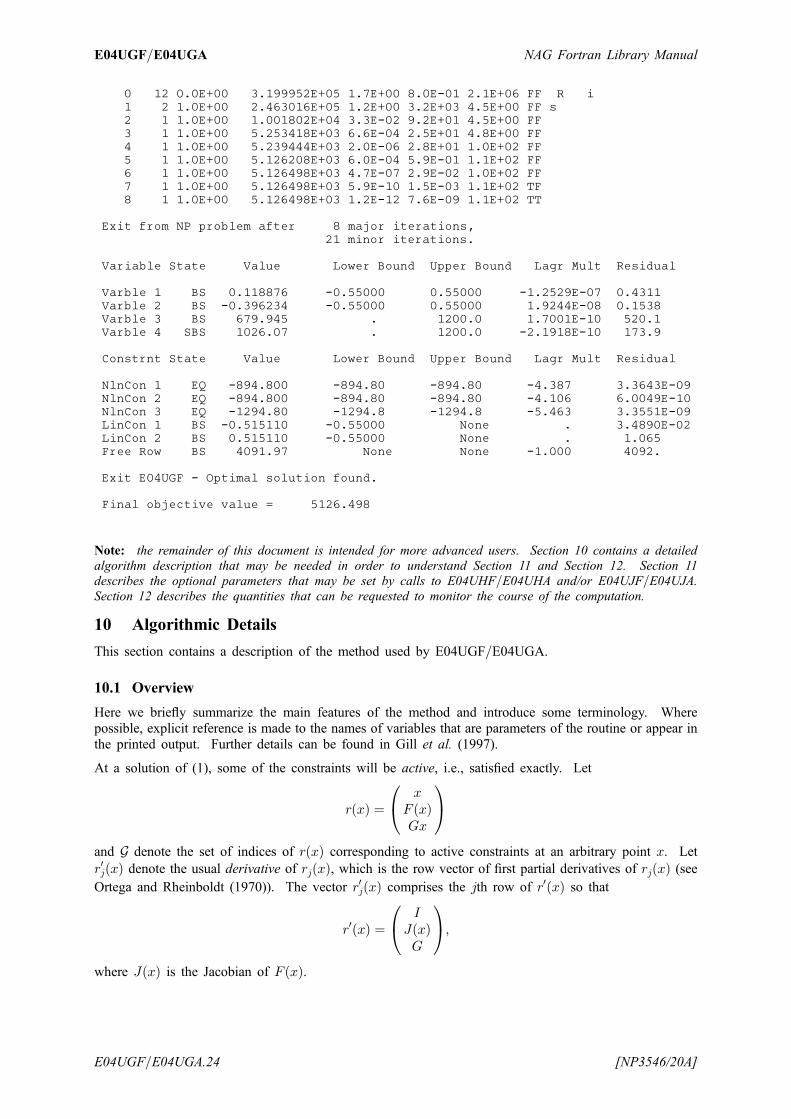
0 12 0.0E+00 3.199952E+05 1.7E+00 8.0E-01 2.1E+06 FF R i1 2 1.0E+00 2.463016E+05 1.2E+00 3.2E+03 4.5E+00 FF s2 1 1.0E+00 1.001802E+04 3.3E-02 9.2E+01 4.5E+00 FF3 1 1.0E+00 5.253418E+03 6.6E-04 2.5E+01 4.8E+00 FF4 1 1.0E+00 5.239444E+03 2.0E-06 2.8E+01 1.0E+02 FF5 1 1.0E+00 5.126208E+03 6.0E-04 5.9E-01 1.1E+02 FF6 1 1.0E+00 5.126498E+03 4.7E-07 2.9E-02 1.0E+02 FF7 1 1.0E+00 5.126498E+03 5.9E-10 1.5E-03 1.1E+02 TF8 1 1.0E+00 5.126498E+03 1.2E-12 7.6E-09 1.1E+02 TT

Exit from NP problem after 8 major iterations,21 minor iterations.

Variable State Value Lower Bound Upper Bound Lagr Mult Residual

Varble 1 BS 0.118876 -0.55000 0.55000 -1.2529E-07 0.4311Varble 2 BS -0.396234 -0.55000 0.55000 1.9244E-08 0.1538Varble 3 BS 679.945 . 1200.0 1.7001E-10 520.1Varble 4 SBS 1026.07 . 1200.0 -2.1918E-10 173.9

Constrnt State Value Lower Bound Upper Bound Lagr Mult Residual

NlnCon 1 EQ -894.800 -894.80 -894.80 -4.387 3.3643E-09NlnCon 2 EQ -894.800 -894.80 -894.80 -4.106 6.0049E-10NlnCon 3 EQ -1294.80 -1294.8 -1294.8 -5.463 3.3551E-09LinCon 1 BS -0.515110 -0.55000 None . 3.4890E-02LinCon 2 BS 0.515110 -0.55000 None . 1.065Free Row BS 4091.97 None None -1.000 4092.

Exit E04UGF - Optimal solution found.

Final objective value = 5126.498

Note: the remainder of this document is intended for more advanced users. Section 10 contains a detailed

algorithm description that may be needed in order to understand Section 11 and Section 12. Section 11

describes the optional parameters that may be set by calls to E04UHF=E04UHA and/or E04UJF=E04UJA.Section 12 describes the quantities that can be requested to monitor the course of the computation.

10 Algorithmic Details

This section contains a description of the method used by E04UGF=E04UGA.

10.1 Overview

Here we briefly summarize the main features of the method and introduce some terminology. Wherepossible, explicit reference is made to the names of variables that are parameters of the routine or appear inthe printed output. Further details can be found in Gill et al. (1997).

At a solution of (1), some of the constraints will be active, i.e., satisfied exactly. Let

rðxÞ ¼x

F ðxÞGx

0@

1A

and G denote the set of indices of rðxÞ corresponding to active constraints at an arbitrary point x. Let

r0jðxÞ denote the usual derivative of rjðxÞ, which is the row vector of first partial derivatives of rjðxÞ (seeOrtega and Rheinboldt (1970)). The vector r0jðxÞ comprises the jth row of r0ðxÞ so that

r0ðxÞ ¼I

JðxÞG

0@

1A;

where JðxÞ is the Jacobian of F ðxÞ.


E04UGF=E04UGA.24 [NP3546/20A]

A point x is a first-order Kuhn–Karesh–Tucker (KKT) point for (1) (see Powell (1974)) if the followingconditions hold:

(a) x is feasible;

(b) there exists a vector � (the Lagrange multiplier vector for the bound and general constraints) suchthat

gðxÞ ¼ r0ðxÞT� ¼ ðI JðxÞT GT Þ�; ð4Þwhere g is the gradient of f evaluated at x;

(c) the Lagrange multiplier �j associated with the jth constraint satisfies �j ¼ 0 if lj < rjðxÞ < uj; �j � 0

if lj ¼ rjðxÞ; �j � 0 if rjðxÞ ¼ uj; and �j can have any value if lj ¼ uj.

An equivalent statement of the condition (4) is

ZTgðxÞ ¼ 0;

where Z is a matrix defined as follows. Consider the set N of vectors orthogonal to the gradients of theactive constraints, i.e.,

N ¼ z j r0jðxÞz ¼ 0 for all j 2 G� �

:

The columns of Z may then be taken as any basis for the vector space N . The vector ZT g is termed thereduced gradient of f at x. Certain additional conditions must be satisfied in order for a first-order KKTpoint to be a solution of (1) (see Powell (1974)).

The basic structure of E04UGF=E04UGA involves major and minor iterations. The major iterationsgenerate a sequence of iterates fxkg that satisfy the linear constraints and converge to a point x� thatsatisfies the first-order KKT optimality conditions. At each iterate a QP subproblem is used to generate asearch direction towards the next iterate (xkþ1). The constraints of the subproblem are formed from thelinear constraints Gx� sL ¼ 0 and the nonlinear constraint linearization

F ðxkÞ þ F 0ðxkÞðx� xkÞ � sN ¼ 0;

where F 0ðxkÞ denotes the Jacobian matrix, whose rows are the first partial derivatives of F ðxÞ evaluated atthe point xk. The QP constraints therefore comprise the m linear constraints

F 0ðxkÞx� sN ¼ �F ðxkÞ þ F 0ðxkÞxk;Gx � sL ¼ 0;

where x and s ¼ ðsN; sLÞT are bounded above and below by u and l as before. If the m by n matrix Aand m element vector b are defined as

A ¼ F 0ðxkÞG

� �and b ¼ �F ðxkÞ þ F 0ðxkÞxk

0

� �;

then the QP subproblem can be written as

minimizex;s

qðxÞ subject to Ax� s ¼ b; l � xs

� �� u; ð5Þ

where qðxÞ is a quadratic approximation to a modified Lagrangian function (see Gill et al. (1997)).

The linear constraint matrix A is stored in the arrays A, HA and KA (see Section 5). This allows you to

specify the sparsity pattern of non-zero elements in F 0ðxÞ and G and to identify any non-zero elements thatremain constant throughout the minimization.

Solving the QP subproblem is itself an iterative procedure, with the minor iterations of an SQP methodbeing the iterations of the QP method. At each minor iteration, the constraints Ax� s ¼ b are(conceptually) partitioned into the form

BxB þ SxS þNxN ¼ b;

where the basis matrix B is square and non-singular. The elements of xB, xS and xN are called the basic,superbasic and nonbasic variables respectively; they are a permutation of the elements of x and s. At aQP solution, the basic and superbasic variables will lie somewhere between their bounds, while the


[NP3546/20A] E04UGF=E04UGA.25

nonbasic variables will be equal to one of their upper or lower bounds. At each minor iteration, xS isregarded as a set of independent variables that are free to move in any desired direction, namely one thatwill improve the value of the QP objective function qðxÞ or sum of infeasibilities (as appropriate). Thebasic variables are then adjusted in order to ensure that (x; s) continues to satisfy Ax� s ¼ b. The numberof superbasic variables (nS say) therefore indicates the number of degrees of freedom remaining after theconstraints have been satisfied. In broad terms, nS is a measure of how nonlinear the problem is. Inparticular, nS will always be zero if there are no nonlinear constraints in (1) and fðxÞ is linear.

If it appears that no improvement can be made with the current definition of B, S and N , a nonbasicvariable is selected to be added to S and the process is repeated with the value of nS increased by one. Atall stages, if a basic or superbasic variable encounters one of its bounds, the variable is made nonbasic andthe value of nS decreased by one.

Associated with each of the m equality constraints Ax� s ¼ b is a dual variable �i. Similarly, eachvariable in ðx; sÞ has an associated reduced gradient dj (also known as a reduced cost). The reduced

gradients for the variables x are the quantities g�AT�, where g is the gradient of the QP objectivefunction qðxÞ; the reduced gradients for the slack variables s are the dual variables �. The QP subproblem(5) is optimal if dj � 0 for all nonbasic variables at their lower bounds, dj � 0 for all nonbasic variables at

their upper bounds and dj ¼ 0 for other variables (including superbasics). In practice, an approximate QP

solution is found by slightly relaxing these conditions on dj (see the description of the optional parameter

Minor Optimality Tolerance).

After a QP subproblem has been solved, new estimates of the solution to (1) are computed using alinesearch on the augmented Lagrangian merit function

Mðx; s; �Þ ¼ fðxÞ � �T ðF ðxÞ � sNÞ þ 12ðF ðxÞ � sNÞTDðF ðxÞ � sNÞ; ð6Þ

where D is a diagonal matrix of penalty parameters. If (xk; sk; �k) denotes the current estimate of thesolution and (xx; ss; ��) denotes the optimal QP solution, the linesearch determines a step �k (where0 < �k � 1) such that the new point

xkþ1

skþ1

�kþ1

0@

1A ¼

xk

sk�k

0@

1Aþ �k

xxk � xkssk � sk��k � �k

0@

1A

produces a sufficient decrease in the merit function (6). When necessary, the penalties in D are increasedby the minimum-norm perturbation that ensures descent for M (see Gill et al. (1992)). As inE04UCF=E04UCA, sN is adjusted to minimize the merit function as a function of s prior to the solution ofthe QP subproblem. Further details can be found in Eldersveld (1991) and Gill et al. (1986).

10.2 Treatment of Constraint Infeasibilities

E04UGF=E04UGA makes explicit allowance for infeasible constraints. Infeasible linear constraints aredetected first by solving a problem of the form

minimizex;v;w

eT ðvþ wÞ subject to l � xGx� vþ w

� �� u; v � 0; w � 0; ð7Þ

where e ¼ ð1; 1; . . . ; 1ÞT . This is equivalent to minimizing the sum of the general linear constraintviolations subject to the simple bounds. (In the linear programming literature, the approach is often calledelastic programming.)

If the linear constraints are infeasible (i.e., v 6¼ 0 or w 6¼ 0), the routine terminates without computing thenonlinear functions.

If the linear constraints are feasible, all subsequent iterates will satisfy the linear constraints. (Such astrategy allows linear constraints to be used to define a region in which fðxÞ and F ðxÞ can be safelyevaluated.) The routine then proceeds to solve (1) as given, using search directions obtained from asequence of QP subproblems (5). Each QP subproblem minimizes a quadratic model of a certainLagrangian function subject to linearized constraints. An augmented Lagrangian merit function (6) isreduced along each search direction to ensure convergence from any starting point.


E04UGF=E04UGA.26 [NP3546/20A]

The routine enters ‘elastic’ mode if the QP subproblem proves to be infeasible or unbounded (or if the dualvariables � for the nonlinear constraints become ‘large’) by solving a problem of the form

minimizex;v;w

�ffðx; v; wÞ subject to l �x

F ðxÞ � vþ wGx

8<:

9=; � u; v � 0; w � 0;

where

�ffðx; v; wÞ ¼ fðxÞ þ �eT ðvþ wÞis called a composite objective and � is a non-negative parameter (the elastic weight). If � is sufficientlylarge, this is equivalent to minimizing the sum of the nonlinear constraint violations subject to the linearconstraints and bounds. A similar l1 formulation of (1) is fundamental to the Sl1QP algorithm of Fletcher(1984). See also Conn (1973).

11 Optional Parameters

Several optional parameters in E04UGF=E04UGA define choices in the problem specification or thealgorithm logic. In order to reduce the number of formal parameters of E04UGF=E04UGA these optionalparameters have associated default values that are appropriate for most problems. Therefore, the user needonly specify those optional parameters whose values are to be different from their default values.

The remainder of this section can be skipped by users who wish to use the default values for all optionalparameters. A complete list of optional parameters and their default values is given in Section 11.1.

Optional parameters may be specified by calling one, or both, of the routines E04UHF=E04UHA andE04UJF=E04UJA prior to a call to E04UGF=E04UGA.

E04UHF=E04UHA reads options from an external options file, with Begin and End as the first and lastlines respectively and each intermediate line defining a single optional parameter. For example,

BeginPrint Level = 5

End

The call

CALL E04UHF (IOPTNS, INFORM)

can then be used to read the file on unit IOPTNS. INFORM will be zero on successful exit.E04UHF=E04UHA should be consulted for a full description of this method of supplying optionalparameters.

E04UJF=E04UJA can be called to supply options directly, one call being necessary for each optionalparameter. For example,

CALL E04UJF (’Print Level = 5’)

E04UJF=E04UJA should be consulted for a full description of this method of supplying optionalparameters.

All optional parameters not specified by the user are set to their default values. Optional parametersspecified by the user are unaltered by E04UGF=E04UGA (unless they define invalid values) and so remainin effect for subsequent calls to E04UGF=E04UGA from the calling program (unless altered by the user).

11.1 Optional parameter checklist and default values

For easy reference, the following list shows all the valid keywords and their default values.

Optional Parameters Default Values

Central Difference IntervalffiffiffiffiffiffiffiffiffiffiffiffiffiffiffiffiffiffiffiffiffiffiffiffiffiffiffiffiffiffiffiffiffiffiffiffiffiffiffiFunction Precision

p

Check Frequency 60Crash Option 0 or 3Crash Tolerance 0.1Defaults


[NP3546/20A] E04UGF=E04UGA.27

Derivative Level 3Derivative/Nonderivative Linesearch Derivative LinesearchElastic Weight 1.0 or 100.0Expand Frequency 10000Factorization Frequency 50 or 100Feasible/Infeasible Exit Infeasible ExitFeasible Point/Maximize/Minimize MinimizeForward Difference Interval

ffiffiffiffiffiffiffiffiffiffiffiffiffiffiffiffiffiffiffiffiffiffiffiffiffiffiffiffiffiffiffiffiffiffiffiffiffiffiffiFunction Precision

p

Function Precision �0:8

Hessian Frequency 99999999Hessian Full/Limited Memory Hessian Full (Limited) Memory if �nn < 75 (otherwise)Hessian Updates 20 or 99999999Infinite Bound Size 1020

Iteration Limit 10000Linesearch Tolerance 0.9List/Nolist List (Nolist for E04UGA)LU Density Tolerance 0:6LU Factor Tolerance 5.0 or 100.0LU Singularity Tolerance �0:67

LU Update Tolerance 5.0 or 10.0Major Feasibility Tolerance

ffiffi�

p

Major Iteration Limit 1000Major Optimality Tolerance

ffiffi�

p

Major Print Level 10 (0 for E04UGA)Major Step Limit 2.0Minor Feasibility Tolerance

ffiffi�

p

Minor Iteration Limit 500Minor Optimality Tolerance

ffiffi�

p

Minor Print Level 0Monitoring File �1Partial Price 1 or 10Pivot Tolerance �0:67

Scale Option 1 or 2Scale Tolerance 0.9Start Objective Check at Column 1Start Constraint Check at Column 1Stop Objective Check at Column n0

1

Stop Constraint Check at Column n001

Superbasics Limit minð500; �nnþ 1ÞUnbounded Objective 1015

Unbounded Step Size maxðbigbnd; 1020ÞVerify Level 0Violation Limit 10.0

11.2 Description of the optional parameters

The following list (in alphabetical order) gives the valid options. For each option, we give the keyword,any essential optional qualifiers, the default value, and the definition. The minimum abbreviation of eachkeyword is underlined. If no characters of an optional qualifier are underlined, the qualifier may beomitted. The letters i and r denote INTEGER and real values required with certain options. The defaultvalue of an option is used whenever the condition jij � 100000000 is satisfied.

Central Difference Interval r Default ¼ffiffiffiffiffiffiffiffiffiffiffiffiffiffiffiffiffiffiffiffiffiffiffiffiffiffiffiffiffiffiffiffiffiffiffiffiffiffiffiFunction Precision3

p

Note that this option does not apply when Derivative Level ¼ 3 (see below).

The value of r is used near an optimal solution in order to obtain more accurate (but more expensive)estimates of gradients. This requires twice as many function evaluations as compared to using forward


E04UGF=E04UGA.28 [NP3546/20A]

differences (see Forward Difference Interval below). The interval used for the jth variable is

hj ¼ rð1þ jxjjÞ. The resulting gradient estimates should be accurate to Oðr2Þ, unless the functions are

badly scaled. The switch to central differences is indicated by c at the end of each line of intermediateprintout produced by the major iterations (see Section 8.1). See Gill et al. (1981) for a discussion of theaccuracy in finite difference approximations.

If r � 0, the default value is used.

Check Frequency i Default ¼ 60

Every ith minor iteration after the most recent basis factorization, a numerical test is made to see if thecurrent solution ðx; sÞ satisfies the general linear constraints (including any linearized nonlinearconstraints). The constraints are of the form Ax� s ¼ b, where s is the set of slack variables. If thelargest element of the residual vector r ¼ b�Axþ s is judged to be too large, the current basis isrefactorized and the basic variables recomputed to satisfy the general constraints more accurately.

If i < 0, the default value is used. If i ¼ 0, the value i ¼ 99999999 is used and effectively no checks aremade.

Crash Option i Default ¼ 0 or 3 (see below)

The default value of i is 0 if there are any nonlinear constraints and 3 otherwise. Note that this optiondoes not apply when START ¼ ’W’ (see Section 5).

If START ¼ ’C’, an internal Crash procedure is used to select an initial basis from various rows andcolumns of the constraint matrix A �Ið Þ. The value of i determines which rows and columns of A areinitially eligible for the basis and how many times the Crash procedure is called. Columns of �I are usedto pad the basis where necessary. The possible choices for i are the following.

i Meaning

0 The initial basis contains only slack variables: B ¼ I.1 The Crash procedure is called once (looking for a triangular basis in all rows and columns of A).2 The Crash procedure is called twice (if there are any nonlinear constraints). The first call looks for a

triangular basis in linear rows and the iteration proceeds with simplex iterations until the linearconstraints are satisfied. The Jacobian is then evaluated for the first major iteration and the Crashprocedure is called again to find a triangular basis in the nonlinear rows (whilst retaining the currentbasis for linear rows).

3 The Crash procedure is called up to three times (if there are any nonlinear constraints). The first twocalls treat linear equality constraints and linear inequality constraints separately. The Jacobian is thenevaluated for the first major iteration and the Crash procedure is called again to find a triangular basisin the nonlinear rows (whilst retaining the current basis for linear rows).

If i < 0 or i > 3, the default value is used.

If i � 1, certain slacks on inequality rows are selected for the basis first. (If i � 2, numerical values areused to exclude slacks that are close to a bound.) The Crash procedure then makes several passes throughthe columns of A, searching for a basis matrix that is essentially triangular. A column is assigned to‘pivot’ on a particular row if the column contains a suitably large element in a row that has not yet beenassigned. (The pivot elements ultimately form the diagonals of the triangular basis.) For remainingunassigned rows, slack variables are inserted to complete the basis.

Crash Tolerance r Default ¼ 0:1

The value r (0 � r < 1) allows the Crash procedure to ignore certain ‘small’ non-zero elements in thecolumns of A while searching for a triangular basis. If amax is the largest element in the jth column, othernon-zeros aij in the column are ignored if jaijj � amax � r.

When r > 0, the basis obtained by the Crash procedure may not be strictly triangular, but it is likely to benon-singular and almost triangular. The intention is to obtain a starting basis containing more columns ofA and fewer (arbitrary) slacks. A feasible solution may be reached earlier on some problems.

If r < 0 or r � 1, the default value is used.


[NP3546/20A] E04UGF=E04UGA.29

Defaults

This special keyword may be used to reset all optional parameters to their default values.

Derivative Level i Default ¼ 3

This parameter indicates which nonlinear function gradients are provided by the user in subroutinesOBJFUN and CONFUN. The possible choices for i are the following.

i Meaning

3 All elements of the objective gradient and the constraint Jacobian are provided.2 All elements of the constraint Jacobian are provided, but some (or all) elements of the objective

gradient are not specified.1 All elements of the objective gradient are provided, but some (or all) elements of the constraint

Jacobian are not specified.0 Some (or all) elements of both the objective gradient and the constraint Jacobian are not specified.

The default value i ¼ 3 should be used whenever possible. It is the most reliable and will usually be themost efficient.

If i ¼ 0 or 2, E04UGF=E04UGA will estimate the unspecified elements of the objective gradient, usingfinite differences. This may simplify the coding of OBJFUN. However, the computation of finitedifference approximations usually increases the total run-time substantially (since a call to OBJFUN isrequired for each unspecified element) and there is less assurance that an acceptable solution will be found.

If i ¼ 0 or 1, E04UGF=E04UGA will approximate unspecified elements of the constraint Jacobian. Foreach column of the Jacobian, one call to CONFUN is needed to estimate all unspecified elements in thatcolumn (if any). For example, if the sparsity pattern of the Jacobian has the form

� � �? ?

� ?� �

0BB@

1CCA

where ‘�’ indicates an element provided by the user and ‘?’ indicates an unspecified element,E04UGF=E04UGA will call CONFUN twice: once to estimate the missing element in column 2 and againto estimate the two missing elements in column 3. (Since columns 1 and 4 are known, they require nocalls to CONFUN.)

At times, central differences are used rather than forward differences, in which case twice as many calls toOBJFUN and CONFUN are needed. (The switch to central differences is not under the user’s control.)


Derivative Linesearch Default ¼ Derivative LinesearchNonderivative Linesearch

At each major iteration, a linesearch is used to improve the value of the Lagrangian merit function (6).The default linesearch uses safeguarded cubic interpolation and requires both function and gradient valuesin order to compute estimates of the step �k. If some analytic derivatives are not provided orNonderivative Linesearch is specified, a linesearch based upon safeguarded quadratic interpolation (whichdoes not require the evaluation or approximation of any gradients) is used instead.

A nonderivative linesearch can be slightly less robust on difficult problems and it is recommended that thedefault be used if the functions and their derivatives can be computed at approximately the same cost. Ifthe gradients are very expensive to compute relative to the functions however, a nonderivative linesearchmay result in a significant decrease in the total run-time.

If Nonderivative Linesearch is selected, E04UGF=E04UGA signals the evaluation of the linesearch bycalling OBJFUN and CONFUN with MODE ¼ 0. Once the linesearch is complete, the nonlinearfunctions are re-evaluated with MODE ¼ 2. If the potential savings offered by a nonderivative linesearchare to be fully realized, it is essential that OBJFUN and CONFUN be coded so that no derivatives arecomputed when MODE ¼ 0.


E04UGF=E04UGA.30 [NP3546/20A]

Elastic Weight r Default ¼ 1:0 or 100.0 (see below)

The default value of r is 100.0 if there are any nonlinear constraints and 1.0 otherwise.

This option defines the initial weight � associated with problem .

At any given major iteration k, elastic mode is entered if the QP subproblem is infeasible or the QP dualvariables (Lagrange multipliers) are larger in magnitude than r� ð1þ kgðxkÞk2Þ, where g is the objective

gradient. In either case, the QP subproblem is re-solved in elastic mode with � ¼ r� ð1þ kgðxkÞk2Þ.Thereafter, � is increased (subject to a maximum allowable value) at any point that is optimal for problem ,but not feasible for problem (1). After the pth increase, � ¼ r� 10p � ð1þ kgðxk1Þk2Þ, where xk1 is the

iterate at which � was first needed.

If r < 0, the default value is used.

Expand Frequency i Default ¼ 10000

This option is part of the EXPAND anti-cycling procedure due to Gill et al. (1989), which is designed tomake progress even on highly degenerate problems.

For linear models, the strategy is to force a positive step at every iteration, at the expense of violating theconstraints by a small amount. Suppose that the value of Minor Feasibility Tolerance (see below) is �.Over a period of i iterations, the feasibility tolerance actually used by E04UGF=E04UGA (i.e., the workingfeasibility tolerance) increases from 0:5� to � (in steps of 0:5�=i).

For nonlinear models, the same procedure is used for iterations in which there is only one superbasicvariable. (Cycling can only occur when the current solution is at a vertex of the feasible region.) Thus,zero steps are allowed if there is more than one superbasic variable, but otherwise positive steps areenforced.

Increasing the value of i helps reduce the number of slightly infeasible nonbasic basic variables (most ofwhich are eliminated during the resetting procedure). However, it also diminishes the freedom to choose alarge pivot element (see Pivot Tolerance below).

If i < 0, the default value is used. If i ¼ 0, the value i ¼ 99999999 is used and effectively no anti-cyclingprocedure is invoked.

Factorization Frequency i Default ¼ 50 or 100 (see below)

The default value of i is 50 if there are any nonlinear constraints and 100 otherwise.

If i > 0, at most i basis changes will occur between factorizations of the basis matrix.

For linear problems, the basis factors are usually updated at every iteration. The default value i ¼ 100 isreasonable for typical problems, particularly those that are extremely sparse and well-scaled.

When the objective function is nonlinear, fewer basis updates will occur as the solution is approached.The number of iterations between basis factorizations will therefore increase. During these iterations a testis made regularly according to the value of Check Frequency (see above) to ensure that the generalconstraints are satisfied. If necessary, the basis will be refactorized before the limit of i updates is reached.

If i � 0, the default value is used.

Feasible Exit Default ¼ Infeasible ExitInfeasible Exit

Note that this option is ignored if the value of Major Iteration Limit (see below) is exceeded, or thelinear constraints are infeasible.

If termination is about to occur at a point that does not satisfy the nonlinear constraints and Feasible Exitis selected, this option requests that additional iterations be performed in order to find a feasible point (ifany) for the nonlinear constraints. This involves solving a feasible point problem in which the objectivefunction is omitted.

Otherwise, this option requests no additional iterations be performed.


[NP3546/20A] E04UGF=E04UGA.31

Feasible PointMaximize Default ¼ MinimizeMinimize

If Feasible Point is selected, this option attempts to find a feasible point (if any) for the nonlinearconstraints by omitting the objective function. It can also be used to check whether the nonlinearconstraints are feasible.

Otherwise, this option specifies the required direction of the optimization. It applies to both linear andnonlinear terms (if any) in the objective function. Note that if two problems are the same except that oneminimizes fðxÞ and the other maximizes �fðxÞ, their solutions will be the same but the signs of the dualvariables �i and the reduced gradients dj will be reversed.

Feasibility Tolerance r Default ¼ffiffi�

p

See Minor Feasibility Tolerance below.

Forward Difference Interval r Default ¼ffiffiffiffiffiffiffiffiffiffiffiffiffiffiffiffiffiffiffiffiffiffiffiffiffiffiffiffiffiffiffiffiffiffiffiffiffiffiffiFunction Precision

p

This option defines an interval used to estimate derivatives by forward differences in the followingcircumstances:

(a) For verifying the objective and/or constraint gradients (see the description of Verify Level below).

(b) For estimating unspecified elements of the objective gradient and/or the constraint Jacobian. Aderivative with respect to xj is estimated by perturbing that element of x to the value xj þ rð1þ jxjjÞand then evaluating fðxÞ and/or F ðxÞ (as appropriate) at the perturbed point. The resulting gradientestimates should be accurate to OðrÞ, unless the functions are badly scaled. Judicious alteration of rmay sometimes lead to greater accuracy. See Gill et al. (1981) for a discussion of the accuracy infinite difference approximations.


Function Precision r Default ¼ �0:8

This parameter defines the relative function precision �R, which is intended to be a measure of the relativeaccuracy with which the nonlinear functions can be computed. For example, if fðxÞ (or FiðxÞ) iscomputed as 1000.56789 for some relevant x and the first 6 significant digits are known to be correct then

the appropriate value for �R would be 10�6.

Ideally the functions fðxÞ or FiðxÞ should have magnitude of order 1. If all functions are substantially lessthan 1 in magnitude, �R should be the absolute precision. For example, if fðxÞ (or FiðxÞ) is computed as

1:23456789� 10�4 for some relevant x and the first 6 significant digits are known to be correct then the

appropriate value for �R would be 10�10.

The choice of �R can be quite complicated for badly scaled problems; see Chapter 8 of Gill et al. (1981)for a discussion of scaling techniques. The default value is appropriate for most simple functions that arecomputed with full accuracy.

In some cases the function values will be the result of extensive computation, possibly involving aniterative procedure that can provide few digits of precision at reasonable cost. Specifying an appropriatevalue of r may therefore lead to savings, by allowing the linesearch procedure to terminate when thedifference between function values along the search direction becomes as small as the absolute error in thevalues.

If r < � or r � 1, the default value is used.

Hessian Frequency i Default ¼ 99999999

This option forces the approximate Hessian formed from i BFGS updates to be reset to the identity matrixupon completion of a major iteration. It is intended to be used in conjunction with Hessian Full Memory(see below).

If i � 0, the default value is used and effectively no resets occur.


E04UGF=E04UGA.32 [NP3546/20A]

Hessian Full Memory Default ¼ see belowHessian Limited Memory

The default is Hessian Full Memory if �nn < 75 and Hessian Limited Memory otherwise.

These options specify the method for storing and updating the quasi-Newton approximation to the Hessianof the Lagrangian function.

If Hessian Full Memory is specified, the approximate Hessian is treated as a dense matrix and BFGSquasi-Newton updates are applied explicitly. This is most efficient when the total number of nonlinearvariables is not too large (say, �nn < 75). In this case, the storage requirement is fixed and you can expect1-step Q-superlinear convergence to the solution.

Hessian Limited Memory should only be specified when �nn is very large. In this case a limited memoryprocedure is used to update a diagonal Hessian approximation Hr a limited number of times. (Updates areaccumulated as a list of vector pairs. They are discarded at regular intervals after Hr has been reset totheir diagonal.)

Note that if Hessian Frequency ¼ 20 (see above) is used in conjunction with Hessian Full Memory, theeffect will be similar to using Hessian Limited Memory in conjunction with Hessian Updates ¼ 20 (seebelow), except that the latter will retain the current diagonal during resets.

Hessian Updates i Default ¼ 20 or 99999999 (see below)

The default value of i is 20 when Hessian Limited Memory is in effect (see above) and 99999999 whenHessian Full Memory (see above) is in effect, in which case no updates are performed.

If Hessian Limited Memory (see above) is selected, this option defines the maximum number of pairs ofHessian update vectors that are to be used to define the quasi-Newton approximate Hessian. Once thelimit of i updates is reached, all but the diagonal elements of the accumulated updates are discarded andthe process starts again. Broadly speaking, the more updates that are stored, the better the quality of theapproximate Hessian. On the other hand, the more vectors that are stored, the greater the cost of each QPiteration.

The default value of i is likely to give a robust algorithm without significant expense, but fasterconvergence may be obtained with far fewer updates (e.g., i ¼ 5).

If i < 0, the default value is used.

Infeasible Exit

See Feasible Exit above.

Infinite Bound Size r Default ¼ 1020

If r > 0, r defines the ‘infinite’ bound bigbnd in the definition of the problem constraints. Any upperbound greater than or equal to bigbnd will be regarded as þ1 (and similarly any lower bound less than orequal to �bigbnd will be regarded as �1).


Iteration Limit i Default ¼ 10000

The value of i specifies the maximum number of minor iterations allowed (i.e., iterations of the simplexmethod or the QP algorithm), summed over all major iterations. (See also Major Iteration Limit andMinor Iteration Limit below.)


Linesearch Tolerance r Default ¼ 0:9

This option controls the accuracy with which a steplength will be located along the direction of search ateach iteration. At the start of each linesearch a target directional derivative for the Lagrangian meritfunction is identified. The value of r therefore determines the accuracy to which this target value isapproximated.


[NP3546/20A] E04UGF=E04UGA.33

The default value r ¼ 0:9 requests an inaccurate search and is appropriate for most problems, particularlythose with any nonlinear constraints.

If the nonlinear functions are cheap to evaluate, a more accurate search may be appropriate; tryr ¼ 0:1; 0:01 or 0.001. The number of major iterations required to solve the problem might decrease.

If the nonlinear functions are expensive to evaluate, a less accurate search may be appropriate. IfDerivative Level ¼ 3 (see above), try r ¼ 0:99. (The number of major iterations required to solve theproblem might increase, but the total number of function evaluations may decrease enough to compensate.)

If Derivative Level < 3, a moderately accurate search may be appropriate; try r ¼ 0:5. Each search will(typically) require only 1� 5 function values, but many function calls will then be needed to estimate themissing gradients for the next iteration.

If r < 0 or r � 1, the default value is used.

List Default for E04UGF ¼ ListNolist Default for E04UGA ¼ Nolist

Normally each optional parameter specification is printed as it is supplied. Nolist may be used to suppressthe printing and List may be used to restore printing.

LU Density Tolerance r1 Default ¼ 0:6LU Singularity Tolerance r2 Default ¼ �0:67

If r1 > 0, r1 defines the density tolerance used during the LU factorization of the basis matrix. Columnsof L and rows of U are formed one at a time and the remaining rows and columns of the basis are alteredappropriately. At any stage, if the density of the remaining matrix exceeds r1, the Markowitz strategy forchoosing pivots is terminated. The remaining matrix is then factorized using a dense LU procedure.Increasing the value of r1 towards unity may give slightly sparser LU factors, with a slight increase infactorization time. If r1 � 0, the default value is used.

If r2 > 0, r2 defines the singularity tolerance used to guard against ill-conditioned basis matrices.Whenever the basis is refactorized, the diagonal elements of U are tested as follows. If jujjj � r2 or

jujjj < r2 �maxi

juijj, the jth column of the basis is replaced by the corresponding slack variable. This is

most likely to occur when START ¼ ’W’ (see Section 5), or at the start of a major iteration. If r2 � 0, thedefault value is used.

In some cases, the Jacobian matrix may converge to values that make the basis exactly singular (e.g., awhole row of the Jacobian matrix could be zero at an optimal solution). Before exact singularity occurs,the basis could become very ill-conditioned and the optimization could progress very slowly (if at all).Setting r2 ¼ 0:00001 (say) may therefore help cause a judicious change of basis in such situations.

LU Factor Tolerance r1 Default ¼ 5:0 or 100:0 (see below)LU Update Tolerance r2 Default ¼ 5:0 or 10:0 (see below)

The default value of r1 is 5.0 if there are any nonlinear constraints and 100.0 otherwise. The default valueof r2 is 5.0 if there are any nonlinear constraints and 10.0 otherwise.

If r1 � 1 and r2 � 1, the values of r1 and r2 affect the stability and sparsity of the basis factorizationB ¼ LU , during refactorization and updating, respectively. The lower triangular matrix L is a product ofmatrices of the form

1

� 1

� �;

where the multipliers � satisfy j�j � ri. Smaller values of ri favour stability, while larger values favoursparsity. The default values of r1 and r2 usually strike a good compromise. For large and relatively denseproblems, setting r1 ¼ 10:0 or 5.0 (say) may give a marked improvement in sparsity without impairingstability to a serious degree. Note that for problems involving band matrices, it may be necessary toreduce r1 and/or r2 in order to achieve stability.

If r1 < 1 or r2 < 1, the appropriate default value is used.


E04UGF=E04UGA.34 [NP3546/20A]

Major Feasibility Tolerance r Default ¼ffiffi�

p

This option specifies how accurately the nonlinear constraints should be satisfied. The default value isappropriate when the linear and nonlinear constraints contain data to approximately that accuracy. A largervalue may be appropriate if some of the problem functions are known to be of low accuracy.

Let rowerr be defined as the maximum nonlinear constraint violation normalized by the size of thesolution. It is required to satisfy

rowerr ¼ maxi

violikðx; sÞk � r;

where violi is the violation of the ith nonlinear constraint.

If r � �, the default value is used.

Major Iteration Limit i Default ¼ 1000

The value of i specifies the maximum number of major iterations allowed before termination. It isintended to guard against an excessive number of linearizations of the nonlinear constraints. Setting i ¼ 0and Major Print Level > 0 (see below) means that the objective and constraint gradients will be checkedif Verify Level > 0 (see below) and the workspace needed to start solving the problem will be computedand printed, but no iterations will be performed.


Major Optimality Tolerance r Default ¼ffiffi�

p

This option specifies the final accuracy of the dual variables. If E04UGF=E04UGA terminates withIFAIL ¼ 0, a primal and dual solution (x; s; �) will have been computed such that

maxgap ¼ maxj

gapjk�k � r;

where gapj is an estimate of the complementarity gap for the jth variable and k�k is a measure of the size

of the QP dual variables (or Lagrange multipliers) given by

k�k ¼ maxffiffiffiffiffim

p ; 1

� �; where ¼

Xmi¼1

j�ij:

It is included to make the tests independent of a scale factor on the objective function. Specifically, gapj is

computed from the final QP solution using the reduced gradients dj ¼ gj � �Taj, where gj is the jthelement of the objective gradient and aj is the associated column of the constraint matrix A �Ið Þ:

gapj ¼dj minðxj � lj; 1Þ if dj � 0;

�dj minðuj � xj; 1Þ if dj < 0:

�


Major Print Level i Default for E04UGF ¼ 10Default for E04UGA ¼ 0

Print Level

The value of i controls the amount of printout produced by the major iterations of E04UGF=E04UGA, asindicated below. A detailed description of the printed output is given in Section 8.1 (summary output ateach major iteration and the final solution) and Section 12 (monitoring information at each major iteration).(See also Minor Print Level, below.)


[NP3546/20A] E04UGF=E04UGA.35

The following printout is sent to the current advisory message unit (as defined by X04ABF):

i Output

0 No output.1 The final solution only.5 One line of summary output (< 80 characters; see Section 8.1) for each major iteration (no printout

of the final solution).� 10 The final solution and one line of summary output for each major iteration.

The following printout is sent to the logical unit number defined by the optional parameter MonitoringFile (see above):

i Output

0 No output.1 The final solution only.5 One long line of output (< 120 characters; see Section 12) for each major iteration (no printout of

the final solution).� 10 The final solution and one long line of output for each major iteration.� 20 The final solution, one long line of output for each major iteration, matrix statistics (initial status of

rows and columns, number of elements, density, biggest and smallest elements, etc.), details of thescale factors resulting from the scaling procedure (if Scale Option ¼ 1 or 2; see below), basisfactorization statistics and details of the initial basis resulting from the Crash procedure (ifSTART ¼ ’C’; see Section 5).

If Major Print Level � 5 and the unit number defined by Monitoring File (see below) is the same as thatdefined by X04ABF then the summary output for each major iteration is suppressed.

Major Step Limit r Default ¼ 2:0

If r > 0; r limits the change in x during a linesearch. It applies to all nonlinear problems once a ‘feasiblesolution’ or ‘feasible subproblem’ has been found.

A linesearch determines a step � in the interval 0 < � � �, where � ¼ 1 if there are any nonlinearconstraints, or the step to the nearest upper or lower bound on x if all the constraints are linear. Normally,the first step attempted is �1 ¼ minð1; �Þ.

In some cases, such as fðxÞ ¼ aebx or fðxÞ ¼ axb, even a moderate change in the elements of x can lead

to floating-point overflow. The parameter r is therefore used to define a step limit �� given by

�� ¼ rð1þ kxk2Þkpk2

;

where p is the search direction and the first evaluation of fðxÞ is made at the (potentially) smaller step

length �1 ¼ minð1; ��; �Þ.Wherever possible, upper and lower bounds on x should be used to prevent evaluation of nonlinearfunctions at meaningless points. The default value r ¼ 2:0 should not affect progress on well-behavedfunctions, but values such as r ¼ 0:1 or 0.01 may be helpful when rapidly varying functions are present.If a small value of r is selected, a ‘good’ starting point may be required. An important application is to theclass of nonlinear least-squares problems.


MaximizeMinimize

See Feasible Point above.

Minor Feasibility Tolerance r Default ¼ffiffi�

p

This option attempts to ensure that all variables eventually satisfy their upper and lower bounds to withinthe tolerance r. Since this includes slack variables, general linear constraints should also be satisfied towithin r. Note that feasibility with respect to nonlinear constraints is judged by the value of MajorFeasibility Tolerance (see above) and not by r.


E04UGF=E04UGA.36 [NP3546/20A]

If the bounds and linear constraints cannot be satisfied to within r, the problem is declared infeasible. LetSinf be the corresponding sum of infeasibilities. If Sinf is quite small, it may be appropriate to raise r bya factor of 10 or 100. Otherwise, some error in the data should be suspected.

If Scale Option � 1 (see below), feasibility is defined in terms of the scaled problem (since it is morelikely to be meaningful).

Nonlinear functions will only be evaluated at points that satisfy the bounds and linear constraints. If thereare regions where a function is undefined, every effort should be made to eliminate these regions from theproblem. For example, if fðx1; x2Þ ¼

ffiffiffiffiffix1

p þ logðx2Þ, it is essential to place lower bounds on both x1 and

x2. If the value r ¼ 10�6 is used, the bounds x1 � 10�5 and x2 � 10�4 might be appropriate. (The logsingularity is more serious; in general, you should attempt to keep x as far away from singularities aspossible.)

In reality, r is used as a feasibility tolerance for satisfying the bounds on x and s in each QP subproblem.If the sum of infeasibilities cannot be reduced to zero, the QP subproblem is declared infeasible and theroutine is then in elastic mode thereafter (with only the linearized nonlinear constraints defined to beelastic). (See also Elastic Weight above.)

If r � �, the default value is used.

Minor Iteration Limit i Default ¼ 500

The value of i specifies the maximum number of iterations allowed between successive linearizations ofthe nonlinear constraints. A value in the range 10 � i � 50 prevents excessive effort being expended onearly major iterations, but allows later QP subproblems to be solved to completion. Note that an extra mminor iterations are allowed if the first QP subproblem to be solved starts with the all-slack basis B ¼ I.(See Crash Option above.)

In general, it is unsafe to specify values as small as i ¼ 1 or 2 (because even when an optimal solution hasbeen reached, a few minor iterations may be needed for the corresponding QP subproblem to be recognisedas optimal).


Minor Optimality Tolerance r Default ¼ffiffi�

p

This option is used to judge optimality for each QP subproblem. Let the QP reduced gradients be

dj ¼ gj � �Taj, where gj is the jth element of the QP gradient, aj is the associated column of the QP

constraint matrix and � is the set of QP dual variables.

By construction, the reduced gradients for basic variables are always zero. The QP subproblem will bedeclared optimal if the reduced gradients for nonbasic variables at their upper or lower bounds satisfy

djk�k � �r or

djk�k � r

respectively, and ifjdjjk�k � r for superbasic variables.

Note that k�k is a measure of the size of the dual variables. It is included to make the tests independent ofa scale factor on the objective function. (The value of k�k actually used is defined in the description forMajor Optimality Tolerance above.)

If the objective is scaled down to be very small, the optimality test reduces to comparing dj against r.


Minor Print Level i Default ¼ 0

The value of i controls the amount of printout produced by the minor iterations of E04UGF=E04UGA (i.e.,the iterations of the quadratic programming algorithm), as indicated below. A detailed description of theprinted output is given in Section 8.2 (summary output at each minor iteration) and Section 12 (monitoringinformation at each minor iteration). (See also Major Print Level above.)

The following printout is sent to the current advisory message unit (as defined by X04ABF):


[NP3546/20A] E04UGF=E04UGA.37

i Output

0 No output.� 1 One line of summary output (< 80 characters; see Section 8.2) for each minor iteration.

The following printout is sent to the logical unit number defined by Monitoring File (see below):

i Output

0 No output.� 1 One long line of output (< 120 characters; see Section 12) for each minor iteration.

If Minor Print Level � 1 and the unit number defined by Monitoring File is the same as that defined byX04ABF then the summary output for each minor iteration is suppressed.

Monitoring File i Default ¼ �1

If i � 0 and Major Print Level � 5 (see above) or i � 0 and Minor Print Level � 1 (see above) thenmonitoring information is produced by E04UGF=E04UGA at every iteration is sent to a file with logicalunit number i. If i < 0 and/or Major Print Level < 5 and Minor Print Level < 1 then no monitoringinformation is produced.

Nonderivative Linesearch

See Derivative Linesearch above.

Optimality Tolerance r Default ¼ffiffi�

p

See Major Optimality Tolerance above.

Partial Price i Default ¼ 1 or 10 (see below)


This option is recommended for large problems that have significantly more variables than constraints (i.e.,n � m). It reduces the work required for each ‘pricing’ operation (i.e., when a nonbasic variable isselected to become superbasic). The possible choices for i are the following.

i Meaning

1 All columns of the constraint matrix A �Ið Þ are searched.� 2 Both A and I are partitioned to give i roughly equal segments Aj; Ij, for j ¼ 1; 2; . . . ; p (modulo p).

If the previous pricing search was successful on Aj; Ij, the next search begins on the segments

Ajþ1; Ijþ1. If a reduced gradient is found that is larger than some dynamic tolerance, the variable

with the largest such reduced gradient (of appropriate sign) is selected to enter the basis. If nothingis found, the search continues on the next segments Ajþ2; Ijþ2 and so on.


Pivot Tolerance r Default ¼ �0:67

If r > 0, r is used during the solution of QP subproblems to prevent columns entering the basis if theywould cause the basis to become almost singular.

When x changes to xþ �p for some specified search direction p, a ‘ratio test’ is used to determine whichelement of x reaches an upper or lower bound first. The corresponding element of p is called the pivotelement. Elements of p are ignored (and therefore cannot be pivot elements) if they are smaller than r.


E04UGF=E04UGA.38 [NP3546/20A]

It is common in practice for two (or more) variables to reach a bound at essentially the same time. In suchcases, the Minor Feasibility Tolerance (see above) provides some freedom to maximize the pivot elementand thereby improve numerical stability. Excessively small values of Minor Feasibility Tolerance shouldtherefore not be specified. To a lesser extent, the Expand Frequency (see above) also provides somefreedom to maximize the pivot element. Excessively large values of Expand Frequency should thereforenot be specified.


Print Level

See Major Print Level above.

Scale Option i Default ¼ 1 or 2 (see below)


This option enables you to scale the variables and constraints using an iterative procedure due to Fourer(1982), which attempts to compute row scales ri and column scales cj such that the scaled matrix

coefficients �aaij ¼ aij � ðcj=riÞ are as close as possible to unity. (The lower and upper bounds on the

variables and slacks for the scaled problem are redefined as �llj ¼ lj=cj and �uuj ¼ uj=cj respectively, wherecj � rj�n if j > n.) The possible choices for i are the following.

i Meaning

0 No scaling is performed. This is recommended if it is known that the elements of x and the constraintmatrix A (along with its Jacobian) never become large (say, > 1000).

1 All linear constraints and variables are scaled. This may improve the overall efficiency of the routineon some problems.

2 All constraints and variables are scaled. Also, an additional scaling is performed that takes intoaccount columns of A �Ið Þ that are fixed or have positive lower bounds or negative upper bounds.

If there are any nonlinear constraints present, the scale factors depend on the Jacobian at the first point thatsatisfies the linear constraints and the upper and lower bounds. The setting i ¼ 2 should therefore be usedonly if a ‘good’ starting point is available and the problem is not highly nonlinear.


Scale Tolerance r Default ¼ 0:9

Note that this option does not apply when Scale Option ¼ 0 (see above).

The value r (0 < r < 1) is used to control the number of scaling passes to be made through the constraintmatrix A. At least 3 (and at most 10) passes will be made. More precisely, let ap denote the largest

column ratio (i.e.,‘ biggest ’ element‘ smallest ’ element

in some sense) after the pth scaling pass through A.

The scaling procedure is terminated if ap � ap�1 � r for some p � 3. Thus, increasing the value of r from0.9 to 0.99 (say) will probably increase the number of passes through A.

If r � 0 or r � 1, the default value is used.

Start Objective Check At Column i1 Default ¼ 1Stop Objective Check At Column i2 Default ¼ n0

1

Start Constraint Check At Column Default ¼ 1Stop Constraint Check At Column Default ¼ n00

1

These keywords take effect only if Verify Level > 0 (see below). They may be used to control theverification of gradient elements computed by OBJFUN and/or Jacobian elements computed by CONFUN.For example, if the first 30 elements of the objective gradient appeared to be correct in an earlier run, sothat only element 31 remains questionable then it is reasonable to specify Start Objective Check AtColumn 31. Similarly for columns of the Jacobian. If the first 30 variables occur nonlinearly in theconstraints but the remaining variables are nonlinear only in the objective, then OBJFUN must set the first30 elements of the array OBJGRD to zero, but these hardly need to be verified. Again it is reasonable tospecify Start Objective Check At Column 31.


[NP3546/20A] E04UGF=E04UGA.39

If i2 � 0 or i2 > n01, the default value is used.

If i1 � 0 or i1 > minðn01; i2Þ, the default value is used.

If i4 � 0 or i4 > n001, the default value is used.

If i3 � 0 or i3 > minðn001; i4Þ, the default value is used.

Superbasics Limit i Default ¼ minð500; �nnþ 1ÞNote that this option does not apply to linear problems.

It places a limit on the storage allocated for superbasic variables. Ideally, the value of i should be setslightly larger than the ‘number of degrees of freedom’ expected at the solution.

For nonlinear problems, the number of degrees of freedom is often called the ‘number of independentvariables’. Normally, the value of i need not be greater than �nnþ 1, but for many problems it may beconsiderably smaller. (This will save storage if �nn is very large.)


Unbounded Objective r1 Default ¼ 1015

Unbounded Step Size r2 Default ¼ maxðbigbnd; 1020ÞThese options are intended to detect unboundedness in nonlinear problems. During the linesearch, theobjective function f is evaluated at points of the form xþ �p, where x and p are fixed and � varies. If jfjexceeds r1 or � exceeds r2, the iterations are terminated and the routine returns with IFAIL ¼ 3.

If singularities are present, unboundedness in fðxÞ may manifest itself by a floating-point overflow duringthe evaluation of fðxþ �pÞ, before the test against r1 can be made.

Unboundedness in x is best avoided by placing finite upper and lower bounds on the variables.

If r1 � 0 or r2 � 0, the appropriate default value is used.

Verify Level i Default ¼ 0

This option refers to finite difference checks on the gradient elements computed by the user-suppliedsubroutines OBJFUN and CONFUN. Gradients are verified at the first point that satisfies the linearconstraints and the upper and lower bounds. Unspecified gradient elements are not checked and hencethey result in no overhead. The possible choices for i are the following.

i Meaning

�1 No checks are performed.0 Only a ‘cheap’ test will be performed, requiring three calls to OBJFUN and two calls to CONFUN.

Note that no checks are carried out if every column of the constraint gradients (Jacobian) contains amissing element.

1 Individual objective gradient elements will be checked using a reliable (but more expensive) test. IfMajor Print Level > 0 (see above), a key of the form OK or BAD? indicates whether or not eachelement appears to be correct.

2 Individual columns of the constraint gradients (Jacobian) will be checked using a reliable (but moreexpensive) test. If Major Print Level > 0 (see above), a key of the form OK or BAD? indicateswhether or not each element appears to be correct.

3 Check both constraint and objective gradients (in that order) as described above for i ¼ 2 and i ¼ 1respectively.

The value i ¼ 3 should be used whenever a new function routine is being developed. The Start and Stopkeywords (see above) may be used to limit the number of nonlinear variables to be checked.

If i < �1 or i > 3, the default value is used.

Violation Limit r Default ¼ 10:0

This option defines an absolute limit on the magnitude of the maximum constraint violation after thelinesearch. Upon completion of the linesearch, the new iterate xkþ1 satisfies the condition


E04UGF=E04UGA.40 [NP3546/20A]

viðxkþ1Þ � r�maxð1; viðx0ÞÞ;where x0 is the point at which the nonlinear constraints are first evaluated and viðxÞ is the ith nonlinearconstraint violation viðxÞ ¼ maxð0; li � FiðxÞ; FiðxÞ � uiÞ.The effect of the violation limit is to restrict the iterates to lie in an expanded feasible region whose sizedepends on the magnitude of r. This makes it possible to keep the iterates within a region where theobjective function is expected to be well-defined and bounded below (or above in the case ofmaximization). If the objective function is bounded below (or above in the case of maximization) for allvalues of the variables, then r may be any large positive value.


12 Description of Monitoring Information

This section describes the intermediate printout and final printout which constitutes the monitoringinformation produced by E04UGF=E04UGA. (See also the description of the optional parametersMonitoring File, Major Print Level and Minor Print Level.) The level of printed output can becontrolled by the user.

When Major Print Level � 20 and Monitoring File � 0, the following line of intermediate printout(< 120 characters) is produced at every major iteration on the unit number specified by Monitoring File.Unless stated otherwise, the values of the quantities printed are those in effect on completion of the giveniteration.

Major is the major iteration count.

Minor is the number of minor iterations required by the feasibility and optimality phases ofthe QP subproblem. Generally, Minor will be 1 in the later iterations, sincetheoretical analysis predicts that the correct active set will be identified near thesolution (see Section 10).

Step is the step �k taken along the computed search direction. On reasonably well-behaved problems, the unit step (i.e., �k ¼ 1) will be taken as the solution isapproached.

nObj is the number of times OBJFUN has been called to evaluate the nonlinear part ofthe objective function. Evaluations needed for the estimation of the gradients byfinite differences are not included. nObj is printed as a guide to the amount of workrequired for the linesearch.

nCon is the number of times CONFUN has been called to evaluate the nonlinearconstraint functions (not printed if NCNLN is zero).

Merit is the value of the augmented Lagrangian merit function (6) at the current iterate.This function will decrease at each iteration unless it was necessary to increase thepenalty parameters (see Section 8.1). As the solution is approached, Merit willconverge to the value of the objective function at the solution.

In elastic mode (see Section 10.2), the merit function is a composite functioninvolving the constraint violations weighted by the value of the optional parameterElastic Weight (default value ¼ 1:0 or 100.0).

If there are no nonlinear constraints present, this entry contains Objective, thevalue of the objective function fðxÞ. In this case, fðxÞ will decrease monotonicallyto its optimal value.

Feasibl is the value of rowerr, the largest element of the scaled nonlinear constraint residualvector defined in the description of the optional parameter Major FeasibilityTolerance. The solution is regarded as ‘feasible’ if Feasibl is less than (or equal

to) the Major Feasibility Tolerance (default value ¼ffiffi�

p). Feasibl will be

approximately zero in the neighbourhood of a solution.


[NP3546/20A] E04UGF=E04UGA.41

If there are no nonlinear constraints present, all iterates are feasible and this entry isnot printed.

Optimal is the value of maxgap, the largest element of the maximum complementarity gapvector defined in the description of the optional parameter Major OptimalityTolerance. The Lagrange multipliers are regarded as ‘optimal’ if Optimal is less

than (or equal to) the Major Optimality Tolerance (default value ¼ffiffi�

p). Optimal

will be approximately zero in the neighbourhood of a solution.

nS is the current number of superbasic variables.

Penalty is the Euclidean norm of the vector of penalty parameters used in the augmentedLagrangian merit function (not printed if NCNLN is zero).

LU is the number of non-zeros representing the basis factors L and U on completion ofthe QP subproblem.

If there are nonlinear constraints present, the basis factorization B ¼ LU iscomputed at the start of the first minor iteration. At this stage, LU ¼ lenLþ lenU,where lenL is the number of subdiagonal elements in the columns of a lowertriangular matrix and lenU is the number of diagonal and superdiagonal elements inthe rows of an upper triangular matrix. As columns of B are replaced during theminor iterations, the value of LU may fluctuate up or down (but in general will tendto increase). As the solution is approached and the number of minor iterationsrequired to solve each QP subproblem decreases towards zero, LU will reflect thenumber of non-zeros in the LU factors at the start of each QP subproblem.

If there are no nonlinear constraints present, refactorization is subject only to thevalue of the optional parameter Factorization Frequency (default value ¼ 50 or100) and hence LU will tend to increase between factorizations.

Swp is the number of columns of the basis matrix B that were swapped with columns ofS in order to improve the condition number of B (not printed if NCNLN is zero).The swaps are determined by an LU factorization of the rectangular matrix

BS ¼ B Sð ÞT , with stability being favoured more than sparsity.



PD is a two-letter indication of the status of the convergence tests involving thefeasibility and optimality of the iterates defined in the descriptions of the optionalparameters Major Feasibility Tolerance and Major Optimality Tolerance. Eachletter is T if the test is satisfied and F otherwise. The tests indicate whether thevalues of Feasibl and Optimal are sufficiently small. For example, TF or TT isprinted if there are no nonlinear constraints present (since all iterates are feasible).If either indicator is F when E04UGF=E04UGA terminates with IFAIL ¼ 0, youshould check the solution carefully.

M is printed if an extra evaluation of OBJFUN and CONFUN was needed in order todefine an acceptable positive-definite quasi-Newton update to the Hessian of theLagrangian. This modification is only performed when there are nonlinearconstraints present.

m is printed if, in addition, it was also necessary to modify the update to include anaugmented Lagrangian term.

s is printed if a self-scaled BFGS (Broyden–Fletcher–Goldfarb–Shanno) update wasperformed. This update is always used when the Hessian approximation is diagonaland hence always follows a Hessian reset.


E04UGF=E04UGA.42 [NP3546/20A]

S is printed if, in addition, it was also necessary to modify the self-scaled update inorder to maintain positive-definiteness.

n is printed if no positive-definite BFGS update could be found, in which case theapproximate Hessian is unchanged from the previous iteration.

r is printed if the approximate Hessian was reset after 10 consecutive major iterationsin which no BFGS update could be made. The diagonal elements of theapproximate Hessian are retained if at least one update has been performed since thelast reset. Otherwise, the approximate Hessian is reset to the identity matrix.

R is printed if the approximate Hessian has been reset by discarding all but itsdiagonal elements. This reset will be forced periodically by the values of theoptional parameters Hessian Frequency (default value ¼ 99999999) and HessianUpdates (default value ¼ 20 or 99999999). However, it may also be necessary toreset an ill-conditioned Hessian from time to time.

l is printed if the change in the norm of the variables was greater than the valuedefined by the optional parameter Major Step Limit (default value ¼ 2:0). If thisoutput occurs frequently during later iterations, it may be worthwhile increasing thevalue of Major Step Limit.

c is printed if central differences have been used to compute the unknown elements ofthe objective and constraint gradients. A switch to central differences is made ifeither the linesearch gives a small step, or x is close to being optimal. In somecases, it may be necessary to re-solve the QP subproblem with the central differencegradient and Jacobian.

u is printed if the QP subproblem was unbounded.

t is printed if the minor iterations were terminated after the number of iterationsspecified by the value of the optional parameter Minor Iteration Limit(default value ¼ 500) was reached.

i is printed if the QP subproblem was infeasible when the routine was not in elasticmode. This event triggers the start of nonlinear elastic mode, which remains ineffect for all subsequent iterations. Once in elastic mode, the QP subproblems areassociated with the elastic problem (see Section 10.2). It is also printed if theminimizer of the elastic subproblem does not satisfy the linearized constraints whenthe routine is already in elastic mode. (In this case, a feasible point for the usualQP subproblem may or may not exist.)

w is printed if a weak solution of the QP subproblem was found.

When Minor Print Level � 1 and Monitoring File � 0, the following line of intermediate printout(< 120 characters) is produced at every minor iteration on the unit number specified by Monitoring File.Unless stated otherwise, the values of the quantities printed are those in effect on completion of the giveniteration.

In the description below, a ‘pricing’ operation is defined to be the process by which a nonbasic variable isselected to become superbasic (in addition to those already in the superbasic set). If the problem is purelylinear, the variable selected will usually become basic immediately (unless it happens to reach its oppositebound and return to the nonbasic set).

Itn is the iteration count.

pp is the partial price indicator. The variable selected by the last pricing operationcame from the pp-th partition of A and �I. Note that pp is reset to zero wheneverthe basis is refactorized.

dj is the value of the reduced gradient (or reduced cost) for the variable selected by thepricing operation at the start of the current iteration.

+SBS is the variable selected by the pricing operation to be added to the superbasic set.

-SBS is the variable chosen to leave the superbasic set. It has become basic if the entryunder -B is non-zero; otherwise it has become nonbasic.


[NP3546/20A] E04UGF=E04UGA.43

-BS is the variable removed from the basis (if any) to become nonbasic.

-B is the variable removed from the basis (if any) to swap with a slack variable madesuperbasic by the latest pricing operation. The swap is done to ensure that there areno superbasic slacks.

Step is the value of the step length � taken along the current search direction p. Thevariables x have just been changed to xþ �p. If a variable is made superbasicduring the current iteration (i.e., +SBS is positive), Step will be the step to thenearest bound. During the optimality phase, the step can be greater than unity onlyif the reduced Hessian is not positive-definite.

Pivot is the rth element of a vector y satisfying By ¼ aq whenever aq (the qth column of

the constraint matrix A �Ið Þ) replaces the rth column of the basis matrix B.Wherever possible, Step is chosen so as to avoid extremely small values of Pivot(since they may cause the basis to be nearly singular). In extreme cases, it may benecessary to increase the value of the optional parameter Pivot Tolerance

(default value ¼ �0:67) to exclude very small elements of y from considerationduring the computation of Step.

Ninf is the number of infeasibilities. This will not increase unless the iterations are inelastic mode. Ninf will be zero during the optimality phase.

Sinf/Objective is the value of the current objective function. If x is infeasible, Sinf gives thevalue of the sum of infeasibilities at the start of the current iteration. It will usuallydecrease at each non-zero value of Step, but may occasionally increase if the valueof Ninf decreases by a factor of 2 or more. However, in elastic mode this entrygives the value of the composite objective function , which will decreasemonotonically at each iteration. If x is feasible, Objective is the value of thecurrent QP objective function.

L is the number of non-zeros in the basis factor L. Immediately after a basisfactorization B ¼ LU , this entry contains lenL. Further non-zeros are added to Lwhen various columns of B are later replaced. (Thus, L increases monotonically.)

U is the number of non-zeros in the basis factor U. Immediately after a basisfactorization B ¼ LU , this entry contains lenU. As columns of B are replaced, thematrix U is maintained explicitly (in sparse form). The value of U may fluctuate upor down; in general, it will tend to increase.

Ncp is the number of compressions required to recover workspace in the data structurefor U. This includes the number of compressions needed during the previous basisfactorization. Normally, Ncp should increase very slowly. If it does not, increaseLENIZ and LENZ by at least Lþ U and rerun E04UGF=E04UGA (possibly usingSTART ¼ ’W’; see Section 5).

The following items are printed only if the problem is nonlinear or the superbasic set is non-empty (i.e., ifthe current solution is nonbasic).

Norm rg is the Euclidean norm of the reduced gradient of the QP objective function. Duringthe optimality phase, this norm will be approximately zero after a unit step.

nS is the current number of superbasic variables.



When Major Print Level � 20 and Monitoring File � 0, the following lines of intermediate printout(< 120 characters) are produced on the unit number specified by Monitoring File whenever the matrix B

or BS ¼ ðB SÞT is factorized prior to solving the next QP subproblem. Gaussian elimination is used to


E04UGF=E04UGA.44 [NP3546/20A]

compute a sparse LU factorization of B or BS, where PLPT is a lower triangular matrix and PUQ is anupper triangular matrix for some permutation matrices P and Q. The factorization is stabilized in themanner described under the optional parameter LU Factor Tolerance (default value ¼ 5:0 or 100.0).

Note that BS may be factorized at the beginning of just some of the major iterations. It is immediatelyfollowed by a factorization of B itself.

Factorize is the factorization count.

Iteration is the iteration count.

Nonlinear is the number of nonlinear variables in the current basis B (not printed if BS isfactorized).

Linear is the number of linear variables in B (not printed if BS is factorized).

Slacks is the number of slack variables in B (not printed if BS is factorized).

Elems is the number of non-zeros in B (not printed if BS is factorized)

Density is the percentage non-zero density of B (not printed if BS is factorized). More

precisely, Density ¼ 100� Elems=ðNonlinearþ Linearþ SlacksÞ2.Compressns is the number of times the data structure holding the partially factorized matrix

needed to be compressed, in order to recover unused workspace. Ideally, it shouldbe zero. If it is more than 3 or 4, increase LENIZ and LENZ and rerunE04UGF=E04UGA (possibly using START ¼ ’W’; see Section 5).

Merit is the average Markowitz merit count for the elements chosen to be the diagonals ofPUQ. Each merit count is defined to be ðc� 1Þðr� 1Þ, where c and r are thenumber of non-zeros in the column and row containing the element at the time it isselected to be the next diagonal. Merit is the average of m such quantities. It givesan indication of how much work was required to preserve sparsity during thefactorization.

lenL is the number of non-zeros in L.

lenU is the number of non-zeros in U .

Increase is the percentage increase in the number of non-zeros in L and U relative to thenumber of non-zeros in B. More precisely, Increase ¼ 100� ðlenLþ lenU�ElemsÞ=Elems.

m is the number of rows in the problem. Note that m ¼ Utþ Ltþ bp.

Ut is the number of triangular rows of B at the top of U .

d1 is the number of columns remaining when the density of the basis matrix beingfactorized reached 0.3.

Lmax is the maximum subdiagonal element in the columns of L. This will not exceed thevalue of the optional parameter LU Factor Tolerance (default value ¼ 5:0 or100.0).

Bmax is the maximum non-zero element in B (not printed if BS is factorized).

BSmax is the maximum non-zero element in BS (not printed if B is factorized).

Umax is the maximum non-zero element in U , excluding elements of B that remain in Uunchanged. (For example, if a slack variable is in the basis, the corresponding rowof B will become a row of U without modification. Elements in such rows will notcontribute to Umax. If the basis is strictly triangular then none of the elements of Bwill contribute and Umax will be zero.)

Ideally, Umax should not be significantly larger than Bmax. If it is several orders ofmagnitude larger, it may be advisable to reset the LU Factor Tolerance to somevalue nearer unity.

Umax is not printed if BS is factorized.


[NP3546/20A] E04UGF=E04UGA.45

Umin is the magnitude of the smallest diagonal element of PUQ.

Growth is the value of the ratio Umax/Bmax, which should not be too large.

Providing Lmax is not large (say < 10:0), the ratio maxðBmax; UmaxÞ=Umin is anestimate of the condition number of B. If this number is extremely large, the basisis nearly singular and some numerical difficulties might occur. (However, an effortis made to avoid near-singularity by using slacks to replace columns of B thatwould have made Umin extremely small and the modified basis is refactorized.)

Lt is the number of triangular columns of B at the left of L.

bp is the size of the ‘bump’ or block to be factorized nontrivially after the triangularrows and columns of B have been removed.

d2 is the number of columns remaining when the density of the basis matrix beingfactorized has reached 0.6.

When Major Print Level � 20, Monitoring File � 0 and Crash Option > 0 (default value ¼ 0 or 3), thefollowing lines of intermediate printout (< 80 characters) are produced on the unit number specified byMonitoring File whenever START ¼ ’C’ (see Section 5). They refer to the number of columns selectedby the Crash procedure during each of several passes through A while searching for a triangular basismatrix.

Slacks is the number of slacks selected initially.

Free cols is the number of free columns in the basis, including those whose bounds are ratherfar apart.

Preferred is the number of ‘preferred’ columns in the basis (i.e., ISTATEðjÞ ¼ 3 for somej � n). It will be a subset of the columns for which ISTATEðjÞ ¼ 3 was specified.

Unit is the number of unit columns in the basis.

Double is the number of columns in the basis containing two non-zeros.

Triangle is the number of triangular columns in the basis with three (or more) non-zeros.

Pad is the number of slacks used to pad the basis (to make it a non-singular triangle).

When Major Print Level ¼ 1 or � 10 and Monitoring File � 0, the following lines of final printout(< 120 characters) are produced on the unit number specified by Monitoring File.

Let xj denote the jth ‘column variable’, for j ¼ 1; 2; . . . ; n. We assume that a typical variable xj has

bounds � � xj � �.

The following describes the printout for each column (or variable). A full stop (.) is printed for anynumerical value that is zero.

Number is the column number j. (This is used internally to refer to xj in the intermediate

output.)

Column gives the name of xj.

State gives the state of xj relative to the bounds � and �.

The various possible states are as follows:

LL xj is nonbasic at its lower limit, �.

UL xj is nonbasic at its upper limit, �.

EQ xj is nonbasic and fixed at the value � ¼ �.


E04UGF=E04UGA.46 [NP3546/20A]

FR xj is nonbasic at some value strictly between its bounds: � < xj < �.

BS xj is basic. Usually � < xj < �.






p).



p).

Activity is the value of xj at the final iterate.

Obj Gradient is the value of gj at the final iterate. (If any xj is infeasible, gj is the gradient of thesum of infeasibilities.)

Lower Bound is the lower bound specified for the variable. None indicates that BLðjÞ � �bigbnd.

Upper Bound is the upper bound specified for the variable. None indicates that BUðjÞ � bigbnd.

Reduced Gradnt is the value of dj at the final iterate.

m + j is the value of mþ j.

General linear constraints take the form l � Ax � u. The ith constraint is therefore of the form

� � aTi x � � and the value of aTi x is called the row activity. Internally, the linear constraints take theform Ax� s ¼ 0, where the slack variables s should satisfy the bounds l � s � u. For the ith ‘row’, it isthe slack variable si that is directly available and it is sometimes convenient to refer to its state. Slacksmay be basic or nonbasic (but not superbasic).

Nonlinear constraints � � FiðxÞ þ aTi x � � are treated similarly, except that the row activity and degree of

infeasibility are computed directly from FiðxÞ þ aTi x rather than from si.

The following describes the printout for each row (or constraint). A full stop (.) is printed for anynumerical value that is zero.

Number is the value of nþ i. (This is used internally to refer to si in the intermediateoutput.)

Row gives the name of the ith row.

State gives the state of the ith row relative to the bounds � and �.

The various possible states are as follows:

LL The row is at its lower limit, �.

UL The row is at its upper limit, �.

EQ The limits are the same ð� ¼ �Þ.BS The constraint is not binding. si is basic.


[NP3546/20A] E04UGF=E04UGA.47






p).



p).

Activity is the value of aTi x (or FiðxÞ þ aTi x for nonlinear rows) at the final iterate.

Slack Activity is the value by which the row differs from its nearest bound. (For the free row (ifany), it is set to Activity.)

Lower Bound is �, the lower bound specified for the ith row. None indicates thatBLðnþ iÞ � �bigbnd.

Upper Bound is �, the upper bound specified for the ith row. None indicates thatBUðnþ iÞ � bigbnd.

Dual Activity is the value of the dual variable �i.

i gives the index i of the ith row.



E04UGF=E04UGA.48 (last) [NP3546/20A]

nag fortran library routine document e04ugf … fortran library routine document e04ugf=e04uga note:...

Documents