Continuum Radiation from Active Galactic Nuclei: A Statistical Study.

(NASA-CE-179925) CONTINUUM RAEIEATXON FROH M87-13368 ACTIVE: G A L A C T I C N U C L E I : A S I B I I S Z I C A L STUDY { E e u n s y l v a n i a S t a t e Uciv.) 8 1 p CSCL 03B

U n c l a s 63/90 44659

192 \\ Takashi Isobel and Eric D. Feigelson ,

Kulinder P. Singh ,

AND

Ajit Kembhavi .

334

4

Rece ived ; accepted

1. Department of Astronomy, The Pennsylvania State University.

2. NSF Presidential Young Investigator.

3. Danish Space Research Institute.

4 . Tata Institute of Fundamental Research.

https://ntrs.nasa.gov/search.jsp?R=19870003935 2018-05-20T12:12:40+00:00Z

t

ABSTRACT

The main purpose of this study is to gain insight into physics of the

continuum spectrum of active galactic nuclei (AGNs) using a large data set and

rigorous statistical methods.

which include radio selected quasars, optically selected quasars, X-ray

selected AGNs, BL Lac objects and optically unidentified compact radio

sources. Each object has measurements of its radio, optical, X-ray core

continuum luminosity, though many of them are upper limits.

sources have extended components, we carefully select out the core component

from the total radio luminosity. With 'survival analysis' statistical

methods, which can treat upper limits correctly, these data can yield better

statistical results than those previously obtained.

We have constructed a database for 469 objects

Since many radio

A variety of statistical tests are preformed, such as the comparison of

the luminosity functions in different subsmples, and linear regressions of

luminosities in different bands. Interpretation of the results leads to the

following tentative conclusions: (1) The main emission mechanism of optically

selected quasars and X-ray selected AGNs is thermal, while that of BL Lac

objects is synchrotron; ( 2 ) radio selected quasars may have two different

emission mechanisms in the X-ray band; ( 3 ) BL Lac objects appear to be special

cases of the radio selected quasars; ( 4 ) some compact radio sources show the

possibility of SSC in the optical band; and (5) the spectral index between the

optical and the X-ray bands depends on the optical luminosity.

- 2 -

I. INTRODUCTION

One of the most important problems in the studies of active galactic

nuclei (AGNs) is understanding the mechanisms of underlying continuum

emission. Although there are already very many observations of AGNs across

the whole range of spectrum, and the knowledge of properties of AGNs has been

improving considerably, we still do not understand the fundamental emission

mechanisms.

combinations of several mechanisms, including both thermal and non-thermal

processes.

radiation. For some objects like BL Lac objects, the synchrotron spectrum

clearly extends to optical region and perhaps to the X-ray band. On the other

hand, most of optically selected quasars do not show radio emission and have

unpolarized continua.

bumps that are not well understood.

combinations of unpolarized synchrotron, bremsstrahlung from an accretion

disk, dust emission, stellar photospheric emission, or Compton scattering by

thermal or non-thermal electrons; In the X-ray band, synchrotron self-Compton

(SSC) is one of the more popular models, though multi-temperature

bremsstruhlung is also probable.

The continuum emission spectrum distributions probably arise from

The radio emission is thought to be incoherent synchrotron

The infrared to ultraviolet regions often have spectral

The emission mechanisms may be

Since the Einstein Observatory has provided high quality X-ray

observations, statistical studies of AGN continua are flourishing (Ku,

Helfand, and Lucy 1 9 8 0 ; Zamorani et al. 1 9 8 1 ; Owen, Helfand, and Spngler 1 9 8 1 ;

Owen and Puschell 1 9 8 2 ; Kriss and Canizares 1 9 8 2 ; Reichert et. al. 1 9 8 2 ;

Zamorani 1 9 8 2 ; Avni and Tananbaum 1982; Blumenthai, Keel, and Miller 1 9 8 2 ;

Kembhavi and Fabian 1982 ; Schwartz and Ku 1 9 8 3 ; Ledden and O'Dell 1 9 8 3 ;

Tananbaum, Wandle, and Zamorani 1983; Katgert, Thuan, and Windhorst 1 9 8 3 ;

Marshall et al. 1983; Bregman 1984; Maccacaro et al. 1984; Henriksen,

Marshall, and Mushotzky 1984; Cruz-Gonzales and Huchra 198rC; Miller 1984;

Marshall et al. 1984; Ledden and O'Dell 1985; Kriss and Canizares 1985; Stocke

et al. 1985; Franceschini, Gioia, and Maccacaro 1986). Considerable attention

has been focused on the evaluation and interpretation of the average optical-

to-X-ray spectral index, <a >, for various samples of AGNs. These finding

are briefly summarized in Table 1. The <a > values have been used, for

example, to infer that radio-selected quasars are several times more X-ray

luminous than optically selected quasars (Ku, Helfand, and Lucy 1980, Zamorani

et al. 19811, that the broad band spectral index evolves with redshift in

radio-quiet quasars (Ku, Helfand, and Lucy 1980, Zamorani et al. 198l), and

that high polarization quasars and BL Lac objects have similar continuum

shapes (Ledden and O'Dell 1985).

ox

ox

In addition to the comparison of broad and spectral indices, statistical

correlations between radio, optical, and X-ray emissions in AGNs have also

been studied by the previous workers. Ku, Helfand, and Lucy (1980) show a

general correlation between radio and X-ray emissions in quasars, which was

confirmed and refined in our examination of radio-loud quasars (Kembhavi,

Feigelson, and Singh 1986; hereafter Paper 11). The close correlation between

optical and X-ray luminosities in Seyferts and quasars has been established by

a number of workers (e.g. Reichert et al. 1982, Blumenthal, Keel, and Miller

1982, Kriss and Canizares 1983, Kriss and Canizares 1985). Zamorani (1984)

and A m i and Tananbaum (1986) have examined the relations between the spectral

index a and optical luminosity and redshift, and Zamorani (1984) has raised

the possiblllty that the quasars X-ray'lminosities are slmultaneously

correlated with their radio and optical luminosities.

ox

- 4 -

. Some researchers have expressed a reluctance to examine directly the

correlations between luminosities at different spectral bands for fear of

encountering spurious correlations, as all luminosities for a given object are

scaled by the same (distance)* factor.

distance-dependent effect occurs if all objects are considered, including

those not detected (Feigelson and Berg 1983 and Paper 11).

this study has been undertaken is that powerful and well-established

statistical techniques are now available that fully account for the presence

of upper limits in luminosity-luminosity diagrams (Feigelson and Nelson 1985,

Isobe, Feigelson, and Nelson 1986).

We have shown, however, that no such

A major reason

The present study represents an improvement upon previous studies in

three respects. First, following Paper 11, we take particular care to

consider CORE radio emission rather than TOTAL radio emission from each AGNs.

The total radio flux frequently includes jets and lobes, which does not

reflect the current state of activity in the nucleus. While this distinction

is small f o r some classes of AGNs (e.g. radio selected BL Lac objects), it is

a considerable correction for others (e.g. 3C and 4C quasars). Note that our

earlier V U observations (Feigelson, Isobe, and Kembhavi 1984; hereafter Paper

I) were specifically designed to acquire radio core fluxes for this study.

Radio observations from certain optically selected quasars not presented in

Paper I, are now presented in 0 11. Second, we analyze a much larger number

of objects than earlier studies by virtue of having collected most or all of

the extant literature. The database ( 0 111) includes all AGNs (except for

certain classes, such as Seyfert galaxies and radio galaxies, where the data

suffer significant anbigilities) f o r vhlch radio core, optical and X-ray

observations have been reported. All upper limits are included. Third, we

use the wide variety of statistical methods provided by 'survival analysis',

- 5 -

the field of applied statistics developed over several decades to solve

problems involving upper limits in medical and industrial situations. These

methods are reviewed in 8 IV; the reader is encouraged to examine Feigelson

and Nelson (1985) and Isobe, Feigelson, and Nelson (1986) for more details.

Applying these statistical methods to the database in § 111, we calculate the

correlations and linear regressions between X-ray, optical, and radio

luminosities. We also investigate several specific issues: (1) The dependence

of optical to X-ray spectral index on the optical luminosity and the redshift;

( 2 ) a proposed two-component model for X-ray emission of the radio selected

quasars; ( 3 ) a comparison of the BL Lac objects with the radio selected

quasars; and (4) a comparison of the optically selected quasars with the X-ray

selected AGNs. The results from these investigation and their interpretations

are presented in § V. 0 VI summarizes the whole study.

- 6 -

11. RADIO OBSERVATIONS

Although most of the data are drawn from the published literatures, we

have made two sets of observations with the NEUO Very Large Array (VU) to

improve the quality of radio data on certain AGNs with measured X-ray

1

luminosities.

The National Radio Astronomy Observatory is operated by Associated

Universities, Inc., under contract with the National Science Foundation.

On 23-24 October 1982, thirty-six optically selected quasars with X-ray

properties measured by Ku, Helfand, and Lucy (1980), or Zamorani et al. (1981)

were observed at the V U . These radio quiet quasars were observed at the same

time as the radio loud quasars discussed in Paper I. The array was in the

standard B configuration and 26 antennas were operating.

given in Table 2a. Twenty-eight quasars were not detected with 5 x rms upper

limits around 1 mJy, and 8 quasars were detected with flux densities between

0.8 and 40.5 mJy. Of these, four were not (to our knowledge) previously known

The results are

radio sources, including the comparatively bright quasars GQ Com and V396 Her.

In the second set of VLA observations, we observed the X-ray selected

AGNs from the serendipitous Einstien IPC sample of Kriss and Canizares (1982).

The observations were performed along with the survey of discussed by Gioia

et al. (1984) on 28-30 November 1981 with the VLA in the C configuration. The

results are given in Table 2b. Data for one object in the sample, 0514-003,

were not good. Snapshots of -12 minutes duration gave 5 x rms upper limits

around 0 .7 mJy for 21 of the sources. Three are detected, one of which

(1401+085, 2-0.43, S -18.8 dy) is quite radio luminous. 5

- 7 -

. I I I. DATABAS E

This study is base on the radio, optical and X-ray luminosities of a

variety of AGNs given in Tables 3, 4 , and 5. In Table 3, we show data on the

radio selected, optically selected, and X-ray selected samples of emission

line AGNs. Data on BL Lacertae type objects are shown in Tables 4a and 4b.

Table 5 includes optically faint o r undetected AGNs for which redshifts

measurements are not available.

The database I however, excludes certain classes of AGNs for which

unambiguous radio cores, optical magnitudes o r X-ray data are not available.

Few Seyfert galaxies have optical core magnitudes reported separately from the

host galaxy brightness, and their radio structures are frequently complex so

that the core is not readily discriminated from ejecta (e.g. Ulvestad and

Wilson 1983).

the diffuse X-ray of the surrounding intercluster medium (Feigelson and Berg

1983), and again optical core magnitudes are usually not available. The PG

sample of bright optically selected quasars (Schmitt and Green 1986, Tananbaum

et al. 1986), the Braccesi and other fields of faint optically selected

quasars (Braccesi et al. 1970, Marshall et al. 1984) have X-ray observations,

but sensitive radio measurements have yet to be published.

samples have therefore been omitted from our study.

Radio galaxy nucleus X-ray emission may be often confused by

All of these

Data in Tables 3 and 4 are organized as follows: Column 1 lists the

source by its Right Ascension and Declination.

name from the various radio and optical surveys. Column 3 gives the redshift

values taken from the X-ray literature, if available, or from other sources

described in the Notes to Tables 3 and 4 . In column 4, we give the radio core

luminosities for the sources. The luminosities are cnmpi-i.ted wir?g the

Column 2 gives the catalog

- 8 -

following formula:

I- 4~ dR 2 f (l+z) (a-1) ,

where a is the spectral index within the appropriate spectral band (f-v-a),

and f is

distance

where we

the observed flux density, z is the redshift and dR is the luminosity

given by cz (1+- l+Z)

2 ' d = -

I Ho assume a Hubble constant HO= 50 Mpc/km/sec and qo==O. For the radio

core emission, we assume the spectral index within the radio band, a -0.

Since many radio selected quasars have extended components, we use the

following procedure to find the core luminosity density at 5 GHz:

i) If a map that

available, the core flux density is used. If the map is not at 5 GHz, the

core spectral index is assumed to be 0.0,

ii) If the source is fully resolved and the core is not detected, we use an

upper limit given in the literature.

density of the weakest component is used as an upper limit.

iii) If an interferometric map is not available, but the source is seen by

single dishes and the spectral index between 1.4 GHz and 5 GHz is less than

0.3, the entire flux density given for the object is assumed to be the core

flux density.

iv) If single dish data are available, and the spectral index is steeper than

0.3, the 5 GHz flux density given for the object is treated as an upper limit,

even if it is detected. This is because of the probable existence of extended

components. Although a distribution of the upper limits set by this procedure

may not be same as that of the upper limits due to the flux Ilmited

observation, we assume that all upper limits belong to a same population. A s

discussed in Paper 11, even such careful efforts to isolate radio core fluxes

r

clearly resolves the core from any jets or lobes is

If an upper limit is not given, the flux

- 9 -

;-

can 1eave.a residual - 50% extra flux from VLBI scale jets. The majority of optically selected quasars and X-ray selected AGNs are

not detected in the radio band. Those that are detected are generally faint

and unresolved, and their flux is assumed to arise from a core with Q -0.0.

Cases where the radio measurement, either detection or upper limit, was made

r

at 2.7 GHz or 1.4 GHz rather than 5 GHz are marked by a * or + in Table 3 .

The optical luminosities are given in column 5 . For optical emission,

the spectral index within the optical band, a -1.0, is assumed. Visual

magnitudes are mainly taken from Hewitt and Burbidge (1980).

magnitudes are converted to the optical luminosity density at 2500 A according

to Zamorani et al. (1981),

0

The visual

log(RO)-37.878 + 2*10g[~(l<)] - 0.4V +- 0.072 corr sin(b)'

where V corr 1968), and the last term is a correction for galactic absorption, where b is

the galactic latitude. If only a blue magnitude is available, the equation is

modified as

is the visual magnitude corrected for MgII line emission (Schmidt

log(~0)-38.011 + 2*log[z(l$)] - 0.48 + 0.072 corr sin(b)'

where Bcorr is the corrected blue magnitude from Schmidt. If a redshift is

not available, an optical flux density at 2500 A at the observer's frame is

computed to find a and a ro ox ' 0.072

log(fo)L19. 756 - Os4' + sin(b)

For some compact radio objects, since only red magnitudes are available, we

need to change the constant in the last equation to -19.521 (Johnson 1966).

Column 6 lists the X-ray luminosities computed for the 0.5-4.5 keV energy

range in the emitting frame and assuming the spectral index within the X-ray

band Q -0.5. The X-ray data are obtained mostly from the observations with

the Einstein Observatory, although some data from observations with the HER.0-1

X

- 10 -

satellite are also included. If the X-ray luminosity in the above energy band

already exists, then it is adopted directly, else it is calculated from the

observed flux in the 0 . 5 - 4 . 5 keV energy band according to the fomulae given

after Table 5 . Column 7 lists the radio spectral index of the core wherever

the measurement exists.

The values for the spectral index (a ) computed between the radio ( 5 ro

GHz) and the optical

column 8.

(2500 A) bands in the emitting frame are listed in

These values are calculated using the following expression:

a -(logRr - logRo)/5.38. ro

If the redshifts are not available, we use the flux densities instead of the

luminosities. The spectral index (aox) between 2500 A and 2 keV emission is given by

a -(logRo - log1 - 17.98)/2.61. ox X

The values for a are listed in column 9. Column 10, 11, and 12 list the

references for the radio, optical, and X-ray data respectively.

ox

Although not shown as separate tables, a few other subsamples are used.

For some statistical problems, we use spatially resolved radio selected

quasars, unresolved radio selected quasars with flat (a <0.3), and steep

(a >0.3) spectra.

r These samples are discussed in detail in Paper 11. r

Comparison of our data calculated luminosities, a and a values to ro ox

previous collection of continuum emission in AGNs, such as Ku, Helfand, and

Lucy (1980), Zamorani et al. (1981), and Ledden and O’Dell (1985), shows

relatively good agreement. One relatively large discrepancy is the radio

luminosity, since we use the core instead of the total luminosities. The

difference in the radio luminosities often reachs an order of magnitude

difference. Because of this, the spectral index between the radio and optical

- 11 -

often show large differences from other studies. This may be due to their

high degree of variability.

There are several possible sources of error in the database. First, data

are collected from variety of references and may be differently treated in

each reference. Second, and related to the first point, uncertainty arises

when a source is variable and observations are not done simultaneously.

Third, some error is caused by the extrapolation of published data with fixed

spectral indices to compute luminosity densities at consistent wavelength in

the emitting frame. For example, this may be an important error source for

the optical luminosity density, since we do not consider the effect of 3000 A

bump and other effects in W region.

sources in VLA maps as cores, VLBI observations often show that the cores can

be resolved to further small scale.

density may be systematically overestimated. Some small errors also arise

from assuming a specific cosmology.

affect correlations, the cosmological constant q does.

Fourth, although we use point radio

Therefore, the core radio luminosity

Although the Hubble constant I f o does not

0

Based on comparisons of luminosities with previous studies and our

estimation of the size of these possible sources of error, we find typical lo

uncertainties of f0.2 in log(R ) , log(Ro), and log(Rx). Although these error

sources may seem large, uncertainties of less than 0 .5 in log form are not

very significant, since the ranges of

r

6 and R are frequently 10 . R r I lo, X

- 12 -

TV i STATISTICAL METHODS

Since the data set contains many upper limits, survival analysis must be

used to treat the data correctly.

lifetime data, is developed over several decades to deal with problems arises

in clinical epidemiology, actuarial science and industrial reliability, where

'censored data' (i.e. upper or lower limits) frequently arise. The methods

are typically extensions of parametric (e.g. least square regression) or non-

parametric (e.g. Kolmogorov-Smirnov or Mann-Whitney tests) statistical tools

used for uncensored data, and frequently involve maximum-likelihood concepts.

Most of the procedures we use in this study are described by Feigelson and

Nelson (1985) and Isobe, Feigelson, and Nelson (1986). The former study

treats problems involving one variable: the Kaplan-Meier estimator is the

maximum-likelihood estimator of the luminosity and gives a mean luminosity and

a standard deviation for a sample; the Gehan and logrank tests measure whether

two subsamples are drawn from a same parent population. The latter study

treats correlation and regression between two variables: Cox regression and

the generalized Kendall's r test (the BHK method) which measure the degree of

independence; the EK algorithm and Buckley-James methods perform linear

regression on the data,

Survival analysis or the analysis of

One new method is used in this study. Previously, we could not fit a line

on a data set which contains upper (or lower) limits in both independent and

dependent variables, except by Schmitt's (1985) method which does not provide

analytic estimates of the uncertainties for the regression parameters. Using

the BHK method described by Isobe, Feigelson, and Nelson (1986), we have

developed a method to find a slope coefficient and uncertainty.

database in two variables (X, Y , ) with possible non-detections in both

Consider a

-c ,

- 13 -

variables. For a range of slope coefficients b , calculate residuals r.=Y -bXi .

The value of b that minimizes the generalized Kendali's T rank correlation

coefficient between the r and X i s the most probable value.

i i

The la

uncertainties can be obtained by finding the slope coefficients which give 31%

of the maximum probability.

Kaplan-Meier estimator. First, get the residuals r with the best slope

coefficient b . The best estimate of the intercept coefficient is the Kaplan-

To find the intercept coefficient, we use the

Meier mean of the residuals. This combination of survival analysis methods on

doubly censored data may permit parameter estimation for non-linear models as

well. We use it in 0 IV to test a two-component model of quasar X-ray

emission.

censored data sets by statisticians (Sen 1968, Efron 1984, Lancaster and Quade

1985), there is no statistical study for censored data sets yet. From our

Although similar procedures have been already suggested for non-

experience, however, the resulting regression coefficients are quite

satisfactory when compared to those obtained by other methods.

Using these survival analysis techniques, we analyze our database. Cox

regression and the BHK method are used to compute the correlation

probabilities between the radio, optical, and X-ray luminosities, and the EM

algorithm and Buckley-James method (and the new linear regression method, if

needed) are used to calculate the linear regression coefficients (0 Va). The

mean values of the spectral indices are calculated by Kaplan-Meier estimator

( 8 V b ) . Multi-dimensional linear regression among the optical luminosity, the

redshift, and the spectral index between the optical and the X-ray bands is

discussed in 0 Vc. The new regression method is applied to analyze the two-

component model for the X-ray emissior. of the radio selected quasars ( § Vc).

For the comparison of the BL Lac objects and the radio selected quasars, and

the comparison of the optically selected and the X-ray selected AGNs, the two

- 14 -

sample tests (Gehan and logrank tests) are used (5 Ve,f).

- 15 -

V. STATISTICAL ANALYSIS AND INTERPRETATION

We now proceed to investigate a number of statistical relations between

the R r , lo, and R

Most of the relationships are illustrated in Figures 1 to 3 , which plot the

values listed for the various samples in Tables 3 to 5. X

luminosity densities against each other, and Figure 4 , which plots the

interband spectral indices a vs. a . The plots are displayed so that the

various subsamples can be easily distinguished.

ox ro

All data lie in the range of 29 < log(Rr) < 3 7 , 28 < log(R ) < 3 3 , 42 <

The radio quasars tend

0

log(Rx) < 4 8 , -0.3 < aro < 1.2, and 0 . 8 < aOX < 1.9.

to occupy higher and relatively wider range (six decades for radio, four

decades for optical and X-ray).

radio quasars.

magnitude weaker than the radio quasars.

range as the optically selected quasars do. The X-ray selected BL Lac objects

are few in number and occupy only two decades in any luminosity; hence we will

not be surprised if significant statistical results are not obtained.

BL Lac objects occupy similar range as the

The optically selected quasars are usually one order of

The X-ray selected AGNs occupy same

a) Correlations and Linear Regressions between AGN Luminosities

Using Cox regression and the BHK method, we establish the significance

level of correlations between radio and X-ray luminosities, optical and X-ray

luminosities, optical and radio luminosities, and a and a for all

subsamples described in 0 111. Quantitative results are shown in Table 6a.

The first column lists the name of the samples and the second column lists the

ro ox

correlations tested. The third column shows the total number of the objects

- 1 6 -

numbers of data points which are censored in the independent variable only,

the dependent variable only, and both the variables, respectively. The fifth

and sixth columns show the correlation probabilities by Cox regression and the

BHK method; This is the probabilities that the two variables are not

correlated with each other. The last column identifies the corresponding

figure. Except for some spectral index correlations, all subsamples show high

significant level between all spectral bands. For example, even the optically

selected quasars show a highly significant correlation (P<O.Ol%) for the radio

and X-ray luminosity relation:

Although we find very high significant levels for nearly all

correlations, it is difficult to tell which correlations are intrinsic and

which correlations are secondary. For a completely detected data set, we can

use a partial linear correlation method and a partial rank correlation, but

these methods cannot treat a censored data set. Using the generalized

Kendall’s 7 correlation coefficient, we may be allowed to use a normal partial

rank correlation formula, but since a partial rank correlation is distribution

free, we cannot get significant levels. We show the partial correlation

coefficients results

qualitative examintion.

shown in Table 7 , but they can be used only for

For the radio selected quasars, the optical / X-ray relation is most

significant (r-0.45, where r is the partial correlation coefficient in Table

7) and the radio / X-ray relation is also important (r-0.42), but the optical

/ radio relation may not be significant (r-0.13). For the optically selected

quasars and the X-ray selected AGNs, the optical / X-ray relation is most

important and two other relations may not be significant. For the radio

selected BL Lac objects, the radio / X-ray relation is most significant and

the optical / X-ray relation is moderately significant, but the optical /

radio relation is weaker. For the X-ray selected BL Lac objects, the optical

/ X-ray relation is most important, and the optical / radio relation is

moderately important, though because of small size of the data, this finding

may not be accurate. We thus find that the Ro / Rx relations are typically of

greatest importance, with the I / R and R / I relations important only in

certain subsamples.

r x r 0

The linear regressions are done mainly by the EM algorithm which assumes

the luminosities are distributed in a Gaussian distribution about the best fit

line, and the Bukley-James method, which makes no assumptions regarding the

distribution of residuals. Since the relation between log(l ) and log(R )

contains upper limits in both variables in the same subsamples, the new method

described in 0 IV is used to compute coefficients. Quantitative results are

shown in Table 6b.

second column lists the independent and the dependent variables. The third

column shows the total number of the objects and the forth column lists the

number of censored data. The fifth and sixth columns show the linear

regression results by the EM algorithm and Buckley-James method respectively.

The first row in the each set shows the intercept coefficient, the second row

shows the slope coefficient, and the last row shows the standard deviation.

If only one set of the result appears, the regression was done by the new

method described in the 0 IV, or by a normal least square method, if there are

no censored data, For example, the radio selected quasars have the linear

regression form, log(Rx)=29.0+(0.48~0.06)log(~ ) . This best fit line is shown

in Figure la.

r X

The first column lists the name of the samples and the

r

The linear regressions can be summarized as follows. The radio/X-ray

correlation is about R aRo*5 for quasars of all types but.is significantly

steeper (R,aR!*8) for BL Lac objects. x r

The optical/X-ray correlation behaves -I L

- 18 -

similarly (RxaR:" for quasars compared to R all'' for BL Lacs), though the x o

X-ray selected AGN subsample does not fit the pattern.

correlation is RraRi*o for the radio and the optical quasars as well as the BL

Lac objects, but, as stated above, may be an indirect consequence of the l

and Ro/lx correlations. The correlation is present in X-ray selected AGNs and

the X-ray selected BL Lac objects, but they have very different forms from the

others.

The radio/optical

J l X

A plausible theoretical interpretation of these results might be as

follow. First, the results of partial correlation analysis (strong

correlation between R

optically selected quasars and the X-ray selected AGNs, the thermal emission

(e.g. bremsstrahlung, Comptonization) is the dominant mechanism. The thermal

emission scale according to I a& (0*7'0'1).

(1983) and Schlosman, Shaham, and Shaviv (1984) for the thermal emission from

accretion disks.

correlation between R and I non-thermal emission is most important. The

non-thermal emission may have the form of R aRr *'O'l). Third, for the radio

selected quasars, the X-ray emission depends on both the radio and optical

emissions.

emission mechanisms (see 8 Vd for the further disccusion).

and Rx but not between R 0 r and Rx) suggest that for the

This form is predicted by Tucker x o

Second, for the BL Lac objects, because of the strong

r X'

X

The result indicates that there are possibly two different X-ray

b) Mean Values of the Spectral Indices

The relation between the interband spectral indices are shown in Figures

4a to 4e with quantitative results given in Table 8 . All mean values and

standard deviations were calculated using the Kaplan-Meier estimator (0 IV).

A s expected from simple selection effects, <a > is relatively large in the ro

- 19 -

radio selected quasars and BL Lac objects, and <aox> is relatively large in

the optically selected quasars.

sources show <a > - 0.5 and <a > > 1.0. On the other hand, the compact

radio sources show <a This means that one power law with

a-1.0 can express the entire emission between the radio and X-ray bands for

this subsample. Close examination of Table 5 also tells that some objects may

have <a > > <a >. Since this relation cannot be readily produced by thermal

or the synchrotron processes, this may be direct evidence for the SSC model

operating in the optical to X-ray bands.

A l l subsamples except the compact radio

ro ox

> - <aox> - 1.0. ro

ro ox

In Table 1, we summarized published values a and a from recent ox ro

literature. A comparison with our results shows that although they are not

exactly the same as our values, they agree reasonably well. For the BL Lac

objects, our results are very similar to Ledden and O'Dell's (1985) results

because of the similar database. We note, however, substantial differences

among different studies of optically selected quasars, ranging from <a

2 0.10 (Marshall et al. 1983) to <aox>11.65 f 0.03 (this study).

Marshall et al. treat lower luminosity objects, this may cause the difference

as we can see in an other study (Zamorani et al. (1981) find for radio quiet

quasars that a

log(Ro)>31.4).

different optical magnitudes (i.e. not those of Hewitt and Burbidge 1980),

frequences at each band (Owen, Helfand, and Spangler 1981, Cruz-Gonzales and

Huchra 1984), selection criteria (Zamorani et al. 1981), correction factors

for absorption and MgII line (Margon, Domes, and Chanan 1985), and different

spectral indices assumed for extrapolations.

h 1 . 3 7 ox

Since

=1.37+0.05/-0.08 for log(Ro)<31.4 but aox -1.62+0.08/-0.11 for

Other possible causes for discrepances are the use of

ox

- 20 -

c) Luminosity Ratio Dependence on Optical Luminosity and Redshift

The dependence of a on optical luminosity and/or redshift for the ox

optically selected quasars is often discussed (Reichert et al. 1982, A m i and

Tananbaum 1982, Zamorani 1982, Maccacaro and Gioia 1983, Zamorani 1984, Kriss

and Canizares 1985, Avni and Tananbaum 1986). Avni and Tananbaum (1982) were

the first to obtain a relation among them using survival analysis (the

"detection-and-bounds1' linear regression method, see Avni and Tananbaum 1986).

Their relation is expressed as

a ox =(-0.0+0.3)(~-0.5)+(0.12~0.06)[1og(Ro)-30.5]+1.50,

where 7 = z/(l+z). They mention that explicit dependence of a on the

optical luminosity is predominant, but the joint dependence of a on both

variables is possible.

and Tananbaum 1986).

ox

ox

This result is confirmed in a more recent paper (Ami

Zamorani (1982) shows a similar relation for a combined sample of

optically selected quasars and Seyfert galaxies.

the redshift, Zamorani (1984) finds

Ignoring the dependence on

. a -0.129 10g(L0)-2.427.

In another subsample, Tanambaum, Wandle, and Zamorani (1983) find a similar ox

relation for radio selected quasars (the 3CR sample),

10~(~~)~27.63+(0.47+0.15)[10~(~~)-31.20]~(0.14~0.12)[10~(~ )-34.781

- (0.45kO. 78) [ log( l+z)-O. 261 . r

Because of the weak dependence on the radio luminosity and the redshift, they

rewrite this relation as

a =0.20 iog(jO)-4.98. ox

We look for analogous relations in our data sets; the results are shown

in Tables 9a and 9b. In Table 9a, we show the relations between a and T and ox

- 21 -

. .

between a and log (lo). Assumed regression forms are a -a+b7 and

a -a+blog(l 1. We find the log(R ) - a slope to be 0.11 f0.02 for radio

selected and optically selected quasars.

show high significance levels for both the redshifts and the optical

luminosity regressions. These relations, however, might be artificial, since

for the optically selected quasars, the optical luminosity is biased due to

optical magnitude limited survey.

selected quasars agrees with the results by Ku, Helfand, and Lucy (1980) and

Zamorani et al. (1981) (see Table 1).

ox ox

ox 0 0 ox

Only the optically selected quasars

The direction of evolution of the optically

We also compute the three dimensional regressions for a 7 , and ox

log(R ) , using the regression form of A m i and Tananbaum (1982). The results

are shown in Table 9b. The second column shows Cox probabilities. The first

value is a joint probability that no correlation exists between a

redshift and log(Ro), the second value is the probability for the redshift

alone, and the third is for optical luminosity density alone. The second and

third values are determined assuming the ratio of the slope coefficient and

the error is distributed as a Gaussian.

results. All subsamples, except the X-ray selected BL Lac objects (P-23%),

show highly significant joint probabilities (P I 0.01%).

selected quasar sample does not show significant correlations for the

individual variables (P(z.)-53% and P(10)=42%), even though this subsample is

the only one which shows high significance levels for correlation between a

and 7 , and a and log(l ) . Although this result does not confirm Avni and

Tananbaum's result which shows that a ox 0

we find similar relations (high joint and individual probabilities) in other

subsamples.

0

and both ox

The third column shows the regression

Only the optically

ox

ox 0

is positively correlated with log(1 ) ,

- 22 -

The interpretation for the radio selected quasars, X-ray selected AGNs,

0 and BL Lac objects is that objects at higher redshifts have higher Rx/R

ratios, and those with higher optical luminosities have lower R R ratios.

For example, a typical radio selected quasar at 2-2 will have a R R ratio

twice that of a similar quasar at 2-0.

selected quasar with log(R )-32 will have a R

JO x / O

At a given redshift, a typical radio

R ratio half that of a similar 0 x / O

quasar with log(R )-33. The slope coefficients in Table 9b can be used to

give analogous results for other subsamples.

0

We also examine the dependence of a on an X-ray luminosity and a ox

redshift.

in Rx as well as a

and the BL Lac objects. Although the X-ray selected AGNs show a high

significance level for both the variables, the BL Lac objects do not.

The results are in Table 9c. Because of the presence of censoring

we can obtain results only for the X-ray selected AGNs ox ’

Comparing these three results, we find some inconsistencies. The radio

quasars, X-ray AGNs, and BL Lac objects show weak positive correlations

between a and 7 in Table 9a, but strong negative correlations in Table 9b.

Table 9c shows another problem. In the relations among a 7 , and log(Rx),

the direction of the dependence on 7 is opposite to that of 7 in the relations

among a on 7 , the

direction should be the same. These inconsistencies suggest that either a

does not truly depend on 7 , or that the evolution is different for the various

wavebands and subsamples.

ox

ox

7 , and log(lo). If there is a real dependence of a ox ’ ox

ox

d) Two Component Model for X-ray Emission of the Radio Selected Quasars

Although an important emission mechanism of the radio selected quasars is

thought to be the synchrotron radiation, the slope of the log(R ) - log(Rx) is r

- 23 -

0.77f0.08 much shallower (Ix -1 o'48'o'06) r than that of BL Lac objects (1 x r -1 > ,

whose emission mechanism is almost certainly the synchrotron.

examination of the plot (Fig. la) shows that the distribution of data points

A close

does not follow a straight line. This has been be interpreted as evidence for

two different types of the radio selected quasars (Owen, Helfand, and

Spangler 1981, Owen and Puschell 1982, and Zamorani 1984).

Zamorani (1984) has suggested that there are two different X-ray emission

mechanisms; for example, a synchrotron component and a thermal component. For

the relation between R and R (see Fig. la), the emission mechanism of the

steeper component at high luminosities would be mainly non-thermal, and that

of the flatter component at lower luminosities would be thermal or a

combination of the non-thermal and thermal emission.

r X

Since if the X-ray

emission is a thermal origin, the X-ray luminosity is expected to be

independent from the radio luminosity. This explanation is supported by the

partial correlation coefficients studied in the 0 Va, since the partial rank

coefficients between the radio luminosity and the X-ray luminosity and that

between the optical luminosity and the X-ray luminosity are equally strong.

The X-ray emission related to the radio luminosity may be a synchrotron or SSC

radiation because of the similarities to the BL Lac objects, and the emission

related to the optical luminosity may be a thermal radiation because of the

similarities to the optically selected quasars.

dimensional regression model with a form of

Zamorani adopts a three

0 br R a 1 + I r , b

x o

He finds that for the flat spectrum radio selected quasars, bo-0.75 and

b -0.95, and for the steep spectral radio selected quasars, bo-0.63 and

b -0 .75. Since the survival analysis cannot treat non-linear problems, we

adopt Zamorani's b-values. Then, using our data set and the application of

r

r

- 2 4 -

the BHK method, we find his equations can be rewritten as

)+21.8,

log( Rx)-log ( l:*63+3x10-7P0 r * 75)+26. 0,

-lORO. 95 r

respectively. The model seems to fit well; however, we found that the

computation of b-values heavily depends on a few points and hence the value is

unstable.

To judge whether this two component model is needed to fit the data, we

compare these models to the other simple models. One is a straight line

(10g(R~)==29.0+0.481og(1~)) and another consists of two straight lines

(10g(1~)-19.0+0.771og(1~) for log(Rr)>33.77 and log(Rx)-45.0 for

log(Rr)<33.77).

components have the same slope coefficient as the BL Lac objects and the flat

components have a zero slope coefficient. The other coefficients are then

found using the BHK method.

The last model is made by assuming that the steeper

2 Since we do not have either a x -test or an other

goodness-of-fit test to compare models for censored data, we need to use a

non-standard method. The Kaplan-Meier estimation of distribution of residuals

found by subtracting these models from the data is examined. The 25th and

75th percentiles of the residuals express the dispersion of the data about the

model. One problem is that these dispersions cannot be translated to

probabilities, and hence the results are only qualitative.

We find dispersions of 0.65, 0.63, 0.51, and 0.44 about the straight line

model, the two straight line model, the flat radio spectra model, and the

steep radio spectra model respectively. Zamorani's (1984) models are thus

better than these other models of the X-ray emission for radio selected

quasars .

Additional support for these composite models is presented in Paper I1

unresolved radio quasars. The subsample of the resolved quasars (with

arcsecond resolution) has a shallower slope (1

subsample of the unresolved quasars (1 -1

with a <0.3; see Fig. 3 in Paper 11). These results are confirmed in our

enlarged data set using survival analysis.

=1°*35'0'04) compared to the x r

71t0 * O7 for the unresolved quasars x r

r

If the X-ray emission mechanism of the resolved radio selected quasars is

dominantly thermal, and that of the unresolved radio selected quasars is non-

thermal, then we can expect a flat slope for the resolved, and a steep slope

for the unresolved radio selected quasars.

e) BL Lac Objects

In our data sets, the radio selected BL Lac objects have a distinct

position.

statistical results are free from the selection effect due to the flux limited

observations. Also because of their nonthermal nature (supported by short

variabilities, high polarizations, and our partial correlation results), they

can be used as a standard to which other subsamples are compared.

Since all the objects are detected in all three frequencies,

Since the BL Lac objects have no upper limits, the partial linear

correlation probabilities in Table 7 can be computed to find which relations

are significant. The partial linear correlation probabilities are

P(rx,o)<O.Ol%, P(ox,r)-2%, and P(ro,x)=20%, where, for instance, P(ro,x) is

the correlation probability between the radio and the optical luminosity for a

fixed X-ray luminosity.

most significant, and the optical/X-ray relation is moderately significant,

but the optical/radio relation is not significant.

The results show that the radio/X-ray relation is

- 26 -

* '

. ' Some researchers have pointed out the s i m i l a r i t i e s between the BL Lac

objec ts and the radio se lec ted quasars. Using two sample t e s t s , we compare

these subsamples. F i r s t , we use a l l da ta i n both the samples. The r e s u l t s

a r e shown i n Table loa.

s e l ec t ed quasars a r e higher than those of the BL Lac ob jec t s , which i s

probably a consequence of the f a c t tha t the radio se lec ted quasars have a much

wider d i s t r i b u t i o n i n the r edsh i f t than the BL Lac objec ts . If the r edsh i f t

range f o r both the subsamples is r e s t r i c t ed t o 0.8 and 1 . 7 , b e t t e r agreements

i n the mean luminosi t ies a r e found (Table lob ) . There a r e , however, some

problems. There a r e only e ight BL Lac objects i n t h i s r e s t r i c t e d sample, and

they do not show any i n t e r n a l radio, o p t i c a l , o r X-ray co r re l a t ions . The

radio se lec ted quasars , i n con t r a s t , give the slope coe f f i c i en t s 0.34+0.10/-

0 .08 f o r log(lr)-log(Rx) and 0.45 f 0.11 f o r log(Ro)-log(Rx), though no

s ign i f i can t r e l a t i o n e x i s t s between log(R ) and log(1 ) . These r e s u l t s can be

in te rpre ted i n two ways.

differences i n the continuum spectra of radio se lec ted quasars and BL Lac

objec ts , and another is t h a t the data a r e too fragmentary t o give firm

conclusions. More BL Lac objects are needed.

The opt ical and the X-ray luminosi t ies of the r ad io

0 r

One in te rpre ta t ion i s t h a t there a r e no s ign i f i can t

The unresolved radio se lec ted quasars a re a l so compared with the BL Lac

objec ts . The samples with r e s t r i c t ed r edsh i f t range show strong s i m i l a r i t i e s .

Therefore the BL Lac objects may be spec ia l cases of the radio se lec ted

quasars.

The d i s t i n c t i v e difference between the radio se l ec t ed and the X-ray

se lec ted BL Lac objects a r e o f t en noted (Ledden and O ' D e l l 1985, Stocke et al.

1985). For example, the mean spectral indices a re : <a >- 0.62 2 0.02,

<a h 1 . 4 6 It 0.03 f o r the radio selected BL Lac ob jec t s , and <a +0.37 f ox ro

0.02 , <a--->l.11 f 0.04 f o r the X- ray se lec ted BL Lac objec ts .

ro

Ledden and UA

- 27 -

O ' D e l l (1985) suggest t h a t the main emission mechanisms of the X-ray BL Lac

objec ts is the synchrotron radiat ion, and the radio selected BL Lac objects

have extra mechanisms, such as beaming.

luminosi t ies of the radio selected and the X-ray se lec ted BL Lac objec ts , we

f i n d t h a t the radio selected BL Lac objects a r e 100 times more luminous than

the X-ray se lec ted BL Lac objects i n the radio band, 7 times more luminous i n

the op t i ca l band, and nearly same i n the X-ray band.

beaming model.

If we compare the averaged

This may support the

But an a l t e rna t ive possible explanation i s a se lec t ion e f f e c t . In the

diagram of Q =box r e l a t ion , we see t h a t the radio se lec ted and the X-ray

se lec ted BL Lac objects mark the lower and upper bounds of the radio selected

quasars.

cases of sources with the same emission mechanism as i n the radio selected

The difference between these two groups may be due t o t w o extreme

quasars.

quasars and the op t i ca l ly selected quasars and the X-ray se lec ted AGNs which

can be a t t r i b u t e d la rge ly t o the select ion methods used i n t h e i r discovery.

If so, w e may f ind "opt ica l ly selected" BL Lac objects somewhere between these

two groups.

and it i s located among the X-ray selected BL Lac objec ts .

f o r high polarized objects ( e . g . Borra and Corriveau 1984) have been generally

unsuccessful.

A s imi la r o f f s e t in the <aro> is seen between the radio selected

Only one BL Lac object was possibly found op t i ca l ly (ZWI 186),

Optical surveys

f ) Comparison of the Optically Selected Quasars and the X-ray Selected AGNs

It is of ten mentioned t h a t the op t i ca l ly se lec ted quasars and the X-ray

se lec ted AGNs have s imi la r natures , and the l a t t e r a r e t r ea t ed as a lower

luminosity sequence o f the former ( e . g . Maccacaro e t al. 1984, Kriss and

- 28 -

Canizares 1985).

between the optical and the X-ray luminosities but do not show the other

relations (see 0 Va). This initially suggests that the X-ray and optical

emission mechanisms of these subsamples are similar. In the plot of log(R )

and log(Rx), however, the slope coefficient of the X-ray selected AGNs are

significantly steeper (0.87 k 0.05) than that of the optically selected

In our data sets, both subsamples show a strong correlation

0

quasars (0.70 f 0.06).

to be shallower (<aox> -1.65 k 0.03) than those of the optically selected

Also the aox indices of the X-ray selected AGNs tend

quasars (<a >-1.35 f 0 1 0 2 ) . The average radio and optical luminosities of ox

the optical selected quasars are about 20 times brighter than those of the X-

ray selected AGNs, but the average X-ray luminosity is nearly the same.

the emission mechanism of these two subsamples were the same, the difference

of the brightness of each band should be approximately same. One explanation

of this difference is suggested by Kriss and Canizares (1985).

the high redshift objects are much ”redder”, since the optical band shifts to

shorter wavelength which I s strongly affected by reddening, while the X-ray

band is not affected much.

quasars which have, on the average, a higher redshift to the X-ray selected

AGNs which have, on the average, a lower redshift, then the optically selected

quasars show more absorption.

If

They show that

Hence, if we compare the optically selected

(g) Groping towards the Physics of AGN Continua

Having investigated the relations between the continua of various types

of AGNs, we should like to know the relevance of the various models of

physical processes of continuum emission to the results of our statistical

“ - “ l . , c b c TI.,.-- --- c..- --.,.-+*ll.. *--- 2:c.C - - - - - L uIu. &&&=LE: a A c ~ ~ ~ L L ~ c ~ ~ ~ c L L L J c w u u A L I e L e : I i L liiecliaI-iisiiis : a chermai

radiation from an accretion disk, and a non-thermal radiation from the

vicinity of the central engine or jets. If the thermal emission from the

accretion disk is the main mechanism (Tucker 1983, Schlosman, Shaham, and

Shaviv 1984), X-ray and optical luminosities may show a correlation but the

radio luminosity is likely to be independent. According to Tucker (1983), the

emission from an optically thick accretion disk can generate the relation

RxccRz with a~0.5 to 0.8. Most of our results are consistent: with this

prediction (a-0.7, except for BL Lac objects where CY - 0.9), though the thermal model does not explain the radio/X-ray correlation seen in most

samples. If the entire continuum is due to synchrotron emission, the X-ray,

optical, and radio luminosities should be well correlated each other with

a ia . All subsamples agree with these conditions. If the synchrotron

self-Compton (SSC) mechanism is important, a strong correlation between the

ox ro

radio and X-ray is expected with a possible correlation with the optical

luminosity through the synchrotron emission. If beaming due to a relativistic

jet exists, it would lead to correlation between all beamed (presumebly

nonthermal) components. Other mechanisms, such as Compton scattering of

blackbody or cyclotron radiation could also be responsible f o r the power low

spectrum in the optical to X-ray bands.

These various models clearly do not make predictions which can be

uniquely distingushed by the R r / R o / l x database studied here.

not sufficiently developed to predict how radio, optical and X-ray

luminosities should scale. Nontheless, we can attempt to reach some crude

conclusions. The fact that Rr is correlated with both R and R in virtually

all subsampies of AGNs (Table 5aj is evidexe against a thermal model for the

continuum spectrum unless, for example, there is some indepedent scaling

between the size of the thermal accretion disk and the strength of the non-

Most models are

0 X

- 30 -

thermal jets.

with a simple or beamed synchrotron model, though models must account for fact

that the scaling between bands is not quite linear (Table 5b). There are no

indications that Rr and 1 are correlated with 1

an SSC model, but this cannot be conclusive evidence against SSC as the

optical band could be dominated by non-thermal continuum (e.g. K8nigl 1981).

The correlation between all three bands is fully consistent

decoupled, as might occur in X 0

Although it is risky to pursue more elaborate models when adjudication

between the simplest ones is difficult, we find the two component AGN

continuum model discussed in 8 Vd is attractive. Here all AGNs have the

thermal emission from the accretion disk and the non-thermal emission from the

jets. The differences between subsamples may be due to the differences

between accretion modes (Blandford 1984). If a radiation torus around a black

hole is radiating at just over the Eddington limit, the emission is dominated

by the thermal radiation, since there are insufficient relativistic electrons

to power a synchrotron continuum. The radio loud quasars accrete at higher

rate so that they produce the jets populated by relativistic electrons, but

the synchrotron emission (and possibly SSC) need not dominate and hence we see

both the thermal disk and non-thermal jet radiations.

be an extreme case with intrinsically luminouse jets and a faint optically

thin accretion disk, or they may possess ordinary jets that happen to be

pointed to us so that the synchrotron emission is extremely enhanced and

dominates the total luminosity.

The BL Lac objects may

There are a few complications in any of these interpretations. One

concern is possible evolution effects.

bands are intrinsically related, then correlations should appear even if the

subsamples are divided into narrow redshift bins within which no evolution

could occur.

If the continuum emission in various

We find most of the RJRyly correlations are present in - - a.

- 31 -

specified bins, but appear weaker than the correlations seen in the entire

subsamples. For example, the correlation probabilities between the radio and

the X-ray luminosities of the radio selected quasars are

0.5, 0.01% for 0.5 I z < 1.0, 0.03% for 1.0 I z < 1.5, 93% for 1.5 5 z < 2.0 ,

17% for 2.0 I z C 2 .5 , and 0.6% for 2.5 5 z. The low correlation

probabilities in these subsamples are partly due to the reduced size of the

data sets in each bin, and partly by the narrow range of luminosities in each

redshift bin.

gives some confidence, however, that the correlations are not entierly due to

cosmological luminosity evolution.

5% for 0.0 5 z <

The existence of the correlations within narrow redshift ranges

Another problem is inappropriately defined samples. We subdivided our

samples by selection criteria such "X-ray selected" or "optically selected"

objects.

samples.

"radio loud" quasars.

statistical results, comparison between the "radio selected" (which are chosen

from their initial discovery in radio surveys) and the "radio loud" subsamples

(which are chosen from the entire sample with the condition a >0.3) shows ro that there is no significant difference.

This method may introduce some mixing of intrinsically different

For example, the optically selected quasars clearly contain a few

Although this mixing might lead to some misleading

We thus find that, although a large number of data were collected, it

proves difficult to specify a physical model. This is partly because most

theoretical studies do not show tracks in a ,Jar, or R / R, / lx plots.

Since these kinds of plots are now widely produced observationally, we

encourage theorists to make such predictions. It is also desirable to have

deeper surveys in all bands so that we can examine samples with wide

luminosity ranges within specific redshift ranges.

the evolution effect on the emission mechanisms.

r

These surveys may clarify

- 32 -

VI. SUMMARY

Using a la rge database, we investigated s t a t i s t i c a l p roper t ies of AGNs

continuum leve ls i n the radio, op t ica l , and X-ray bands. For the radio

luminosity of AGNs, we used the core luminosity t o discount e f f e c t s from radio

lobes and j e t s . The s t a t i s t i c a l methods ca l l ed survival analysis were used t o

show the s t a t i s t i c a l r e l a t ions despite the upper l i m i t s i n f lux l imited data

s e t s . Our main r e s u l t s are as follows:

1. For the op t i ca l ly se lec ted quasars and the X-ray se lec ted AGNs, R is

cor re la ted with R does not co r re l a t e with R . X' r X

suggests t h a t the main emission mechanism of these subsamples i s thermal

emission.

t h i s suggests t h a t the main emission mechanism of the BL Lac objects i s non-

thermal. The radio selected quasars show high s ignif icance leve ls fo r both

R R and R R r e l a t ions . Hence they may have both the mechanisms, which is

fu r the r supported by model f i t t i n g suggesting t h a t the radio se lec ted quasars

have two d i f f e r e n t X-ray emission mechanisms.

2 . The BL Lac objec ts have s imilar emission mechanisms as the radio selected

quasars, a t l e a s t i n the l imited redshi f t range overlapping both samples. The

radio se lec ted BL Lac objects a re perhaps spec ia l cases of the unresolved

radio se lec ted quasars. The difference between the radio se lec ted and the X -

ray se lec ted BL Lac objects may be due e i t h e r t o beaming e f f e c t s o r se lec t ion

e f f e c t s .

3 . Some compact radio sources with f a i n t op t i ca l counterparts show t h a t

<a > 2 <a >. This suggests the poss ib i i i t y t ha t SSC emission may be present

i n the op t i ca l t o X-ray bands.

4 . The spec t r a l index between the opt ica l and X-ray luminosi t ies depends on

0

but not with Rr. Also R This

For the BL Lac objec ts , Ir/Rx r e l a t i o n is most s i g n i f i c a n t , and

I / X J X

ro ox

- 33 -

the optical luminosity.

ray luminosity.

The optical luminosity increases faster than the X-

- 34 -

Acknowledgements

We would like to thank D. J. Helfand and H. KGhr for providing

unpublished data. One of us (K. P. S.) would like to thank Prof. G. P.

Garmire for the hospitality at the Pennsylvania State University while working

on this study. This work was supported in part by NASA grant NAG 8 - 5 5 5 and by

a NSF Presidential Young Investigator Award (AST 8 3 - 5 1 4 4 7 ) .

- 35 -

Table Captions

Notes t o Table 2a:

1. F i r s t detected by Condon and Dressel (1978). We f i n d a f a i n t radio

lobe (3 d y ) 6" a t P . A . 104 ' from the quasar.

2 . A 6xRMS detec t ion within 1" of the op t i ca l pos i t ion .

3. A 5.5xRMS detec t ion within 1" o f the op t i ca l pos i t ion . Mrk 205 was

a l s o detected by Sulent ic (1986) a t a l eve l of 1.48 2 0.25 mJy

a t 5 GHz.

4. F i r s t detected by Sramek and Weedman (1980). Our improved pos i t i on i s

12h58m59.4s, 34'16'38".

5 . A 7xRMS detec t ion within 1" of the op t i ca l pos i t ion .

6. F i r s t detected by Sramek and Weedman (1980). Our improved pos i t ion is

16h04m53.4s, 29'03'21".

Definit ions f o r Table 3:

Optical

If a r ad io AGN has an op t i ca l "empty f i e l d " , D 2 0 . 0 is used as the op t i ca l

upper l i m i t .

X-ray

If only the X-ray f l u x (or f l u x density o r count number) i s ava i l ab le , the

luminosity i s computed according t o the descr ipt ions below f o r the given

reference:

* L1 X-ray l i s t gives X-ray data i n the f lux densi ty a t 1 keV. The conversion

t o the f l u x (0.5-4.5 keV) i s

- 36 -

S (0.5-4.5) [ erg/sec/cm 2 ]=O. 068 fx( IkeV) nJy X

* 01 X-ray list gives the X-ray data in the flux (0.15-3.5 keV). The conversion is

S (0.5-4.5)=0.95 Sx(0.15-3.5) X

* B3 X-ray list gives the X-ray (0.5-3.0 keV flux). The conversion is

S (0.5-4.5)=1.38 Sx(0.5-3.0). X

* G2 X-ray list gives the X-ray (0.3-3.5 keV flux). The conversion is

Sx(0.5-4.5)-1.07 Sx(0.3-3.5).

* W2 X-ray list gives the X-ray K count rate. The conversion is 2

sX=2. 8 8 x ~ ~ - 1 3 ~ 2 erg/sec/cm 2 .

* The X-ray flux is computed from Einstein IPC photon counts (cts/sec) by

1.01~~(cts/sec)-3. o ~ I o - ~ ~ erg/sec/cm 2

assuming N(H)-3xlO 20 cm -2 and S -(freq) -0.5

* The X-ray flux density at 2KeV is computed by

2 Sx( 2KeV)=1. 47x10-18f erg/sec/cm

x El o.5-E20.5

where El and E2 are the band limits in KeV and f is in erg/sec/cm 2 . X

Notes to Table 8 :

1. Data have too many upper limits and the result is obtained from

a limited range.

- 37 -

Table 1 : Spectral Indices from Recent L i t e ra tu re s

Study Spectral Indices Descriptions

Tananbaum et al. a -1.27fO.07 Mixed QSOs ox

(1979)

Ku et al. (1980) a -1.46k0.02 Total sample ox

a -1.38fO.03 Radio se lec ted QSOs

a -1.52+_0.03 Optical ly se lec ted QSOs

a -1.41fO.03 X-ray selected AGNs

a -1.36kO.04 Radio QSOs with low redsh i f t ( ~ ~ 1 . 0 )

a -1.40f0.03 Radio QSOs with high redshif t (z>l .O)

a -1.36fO.04 Opt. QSOs with low redsh i f t (z<l.O)

a -1.65f0.04 Opt. QSOs with high r edsh i f t (z>l.O)

a -1.25f0.05 ow

a -1.31f0.05 EL Lacs

ox

ox

ox

ox

ox

ox

ox

ox

ox

Zamorani et al. a -1.27f0.03 Radio loud ox

a -1.46+0.05/-0.07 Radio qu ie t

a -1.35+0.05/-0.08 Radio qu ie t with low redsh i f t ( ~ ~ 1 . 0 )

a

a

a

ox (1981)

ox

-1.62+0.08/-0.16 Radio qu ie t with high r edsh i f t ( ~ 1 . 0 )

=1.37+0.05/-0.08 Radio quie t with log(Ro)<31.4

=1.62+0.08/-0.11 Radio qu ie t with log(1 )>31.4

ox

ox

ox 0

Owen et al. (1981) a -1.02f0.05 nun selected AGNs

a -1.21f0.19 mm se lec ted AGNs

mx

ox

Stocke et al . (1983) aox=1.3?0.2

Marshall et al.

X-ray se lec ted AGNs

a =1.37k0.10 Optical ly se lec ted quasars ox

(1983)

- 38 -

Cruz-Gonzales and a -0.59k0.10

a -0.94kO.09 Huchra (1984)

Margon and Chanan aox=1.26+0.03

ri

rx

(1985)

Ledden and O'Dell a -0.63kO.12

a -0.89kO.06

a -1.40k0.17

a -0.74f0.10

a -0.92k0.06

a -1.30+0.13

a -0.67kO.12

a -1.36kO.17

ro

rx (1985)

ox

ro

rx

ox

ro

ox

BL Lac : radio - inf ra red

BL Lac : radio - X-ray

X-ray selected quasars

BL Lacs

BL Lacs

BL Lacs

HPQs

HPQs

HPQs

Blazars

Blazars

- 39 -

Table 2a : VLA Observations of Optically Selected Quasars

Object Name S6(mJy) Note Object Name S6(mJy) Note

0137-010 NAB

0143-015 MC5 366

0143-010 MC5 368

0146+017 MC5 141

0207 - 378 0241+011a nrNGC1073

0241+011b nrNGC1073

0241+011c nrNGC1073

0242-410

0849+154 LB 8796

0854+194 Ll3 8948

0855+188 LJ3 8991

0856+186 LB 9010

0856+189 LB 9029

1045+128a nrNGC3384

1045+128b nrNGC3384

1045+128c nrNGC3384

1045+128d nrNGC3384

<0.8

<0.8

<0.8

4 . 2

<1.3

c2.0

<2.0

40.5

<1.4

<0.9

1.8

<0.9

<1.0

<0.8

4 . 0

<0.9

<0.9

<1.0

1

1045+128e

1045+12 8 f

1045+128g

1045+128h

1202+28 1

1219+7 5 5

1246-057

1258+286

1258+342

1300- 243

1334+286

1346 -036

1604+2 90

1606+288

1606+289

1720+246

1803+676

2225-055

nrNGC3 384

nrNGC3 3 84

nrNGC3384

nrNGC3 384

GQ Com

Mrk 205

W 61972

K P 33

RS 23

KP 63

KP 64

K P 67

V396 Her

PHL 5200

4 . 1

<0.9

<0.9

4 . 0

1.1

0.9

<0.9

<0.9

25.1

1.3

<0.8

4 . 0

4.0

<0.9

<0.9

31.0

<0.8

<0.8

2

3

4

5

6

Table 2b : VLA Observat ions of X-ray S e l e c t e d AGNs .

Ob jec t N a m e s6 (&y) Objec t N a m e '6 (mJy)

0057+311

0112+325

022 5+3 12

0 244+19 2

03 5 7+104

0745+554

0 7 54+3 9 2

09 0 6+42 5

1008+345

1011+0 3 2

10 3 1+5 8 2

1139+104

1E

1 E

1E

1E

1 E .

1 E

1 E

1 E

1 E

1 E

1 E

1 E

<0.7

<0 .8

<0.6

~ 0 . 6

<0.7

~ 0 . 7

3 .6

<0.8

<0.8

<0.7

<0 .6

4 . 1

1205+46 5

1 2 2 8+164

1 3 04+3 4 1

135 2+1820

1352+1828

1357-022

1401+09 5

1 5 29+050

1 5 30+15 1

1602+241

1747+6 8 3

2251-175

1E <0.7

1E <0.8

1 E <0.7

1 E <0.7

1E 4 . 0

1 E <0.7

1E 1 8 . 8

1E 3 . 8

1 E <0 .9

1E < 1 . 2

1E <0.6

1 E <0 .7

- 41 -

. *

cd k U 0 Q a VI

9 63 4 U c 0 u

.. m

v) & cd v)

a Q) u - 0 Q -1

n cd v

Y ) m m m o D m r - m u m 00000 v v v v N 4 h o m * . .

. . . . .

i o 0 : :

0 o m . D m ' O - Y o u w - - r ( o u + + + + + o - - l r ) m u l n o o o - - m m w 00000

- 4 2 -

O W - t h O w m - T c v V I . . . . .

4 4 6 4 4 A A A A

O N N I n 4 u O O V 0

0 0 0 0 0 v v v v

00000 m u m N N t.l d N o m u . . . . .

a al

h rl d (d c) d U n

(d f+ h

0 n

e e t ~ m m m h r l m m m m o m w m m h U m O w u m m m

v v v v '91'91':

0 0 0 0 0 0 0 0 0 0 00000

O N N W N do N L n m m m Y ) o m m r ( O N . . W 4 N O fCl

00004 0 0 . .o O?? ' ? . . . . . . . . . . . . . .

O N

0, . . N N O U h

N e44 d V U N U

m m o

m u m u 8

d

- 4 3 -

. .

o u m o o ? ? ? ? ? r(d.-dd A A A A m d O N O d * O N N

0 0 0 0 0 v v v . . . . . Ouod.4

O O N O 4

v v v v v 00000

r - m o m u

mU)\O.n.D u u u u u v v v v

Q!????

0 -4

z -4

N

4

8

z

Y o

*

- 0 0 0 0 0 m o I D o

r ( d d O N T T ? ? ?

o o m o r - o o m r - u 0 o o u u . 4

m m . - o m w a r - h r o N N N N N + + + + + N N O O O N N N N N W W W W l D L-ldr(drl :

U

u ~ m m m m u O d N

a v v v v e 00000 m h r o u m

0 0 0 0 0 v v v ??-!??

m d O u N O d N N N

0 0 0 0 0 v v v v . . . . . ~ ~ m m d

v v v ?-!??? y , o o o o ~ N N O ~ m r - d m 1 . f

? ? O d N . . . . . . . . o m o u m o o y o o 0 0 0 0 0 v v v v v v v v v

u ~ o m r - o m m m u o u m o m N N M A ~ m u m a m \ O W \ O W O v ) u u u u u u u u u u v v v v v v v

. . . . . . . . . .

- 4 4 -

R % g % g d O d W N

O N N N N . . . . .

m o u o o r o r c ~ m u

-!???? O O O N d

N

. -

w o a m u O N N O d

2 0 0 0 0 0 a v v v v

o m o m n n ??1-!? o o o o g v v v v v

O d N N I - o m y o 0 0 0 0 0 0 v v v v

m h u m o N 4 d O l

00000 v v v v v . . . . .

I D I n U U N O O N - O

v v d m C N m N u U d u m e 0 N u u u < u

. . . . . o p o o o

. . . . .

O O I N N h

Q I o m m m N O N N N

m m w - ~ . . . . .

c l m o o u O O O " ( V

0 0 0 0 0 v v v v v O N rou -ode-¶

v u u u u

. . . . .

. . . . . u r o n ~ ~ u

u o o u m -"\Dm . . . . .

u m - o m u a o m m m o o m m v v v v v

. . . . . N O O N N

w m m w m r o h + d v ) N O N m d O O O N 0 v v v v

. . . . . r o m o o m - w a r n 0 . . . . . :z4zz 4x2g;:

v v v

N U N 0 0

0 0 0 0 0 . . . . . u) O PI

m w m m m m o m m m O N W O O . . . . .

( I O N N O v v v v v

O d O O O . . . . . o u m - p . . n C u r o m m N O O O O

.d a

. . . . . m o o o m N O r n O N v v v v v

d s z u O o m m u d m u m d O N N O

0 0 0 0 0 . . . . .

00000 0 0 0 0 0 O O d O d 0 d

8 c. W W W W Y W W W W W d

cd c3

W W W W W W W W W W P W W W W W Y W W W W Y W W Y W W W W W

$

9 .I4

V

a a u 0 a rl a VI

h rd $4

;e n 0 W

0r1d-o m m o m o N N N ~ ~ " i 0 0 0 ~ 0 O O ? " i ? - 0 o o - J . o g o o o ? O O O O 0 0 0 0 0 v v v v v v v v v v v v v

d \ D N O O W N b O W . . . . . 4444s: v v v v w l r m o o m m N m m N d N W O

O O O d O

U m O N

. . . . .

O N w m O m u m - 0 O m m O N O N N O O v v v v

r n + u w m O d - n Y l

. . . . .

O d d O U ,

o o o a o . . . .

0 w C l l - m

d 0 d O O L ~ O ~ C I O

0000r; - d CI

c

c. W W W W W W W W i 2 I i W W W W W W W W W W W W W W W W W W W W W W W Y W W W W W W

- O h m - - - - ? . -

m u m m m d N N d 0 O O O O N

I + + I I - m a o o o u O O m m u 00000 00000

c; '???? -ddNr. O O O O O 00000 0 0 0 0 0

-45 -

4 U G 0 u I

n u

pr)

al rl

W

P a k

0

a

U 0

2 0

u 0 9)

..

a al u L al

I 4 al

LA

0

n cd W

OlcNdDVI ? ? - ? ? V I

O d W h 0 h W W m W

00000 . . . . .

o . . . . . . . . . . . . - 0 0

N 0 0 h r( m h w u 2 ? ? m . O W - . N . . . .- -l . . . .it m u . r ( . u . o m m . * . . .

0 O m O (1 0Oi- l 0

m u~ w

d 00 0 0 O N 0 0

W .o

0

. . . . .u e m . u s m . 2 m g . 2 . . . . . . . . . . . . . . . . . :-? : : : :7 N . . . . W -3- . O . W ' 0 - 0

- 4 6 -

m x 4 00 .A - Fl

e 0 4 4 L - J - 4

0000 0 "I??? 7

4 0

. . . i t . w u u : : ? : ? :

w w

. . m . o N r ?

: : ? : Y 0 _c

0 - 4

. . 4 . N m o

: : ? : "I (d $4 c, c) P) CL v1

N *

vl u 4

- V I < O

a-B 2 W U Z Y

B = w

L P)

0 2 4 u u

0 0 a + N 2 % 4

c) (d I4

g v1

0

Q) v)

2 k a

6 u x e n $4

0)

0 s .. m

IC 01 o w 0- m u . a . m u m o m

0 0 0 00000 N 4.4 . . : ? : ? ? ? ? ?

-47-

m 0 xc 0 .T )u

0 6 0) 0 9

a m u u 0

n u

m m a 9 . n

m a l Y Y 0 0 v u a m 5 5 N

0 0 u u 0 U 2 - > . . .

m O W d ,-Id

,-I 4.4 .4 4.4

6 64

t . & t

G O N c 5 x s u m u r v - 4 2 d E B ~ E u a u u 0 N 0 0 0 N N

m m m

u u u u 0 0 0 4

W u u u 6 u m m x x x u o u u 4 0 4 4 u > u m c - c c m o O O Q m Q 0

3 % d m d d . W 4 W W O M

0 0 0 0 0

. a l a m a l Y Y Y Y E

m a e m u u u u * w

'FFl5F a4

5 c c

9 3 u u 2 m 4

m u 4 4

rA

a C a

1 1 1 1 1 1 1 1 1 1 1 1 1 1 1 1 1 1 1

4

m a G a

N m m .4

m al

4 . . . . . . . . . . . . . . . . . . . . . . . . . . . . . . . . . . . . . . . . . . m

Ll 0 cu

m al

m u L) al 0 u a"

m 4 4 u

m u r n o m 0 3

e a 99

2 0 rl

m 0) 0 c 4

z1

m al u 0 z

r4 > . I

U

0, ,-l m

. . . . . . . . . . . . . . . . . . . . . . . . " d . . . . . . . . . . . . . . . . . .

-48-

Y a U m

e o 0 I , * 0 0 0 u u u U Q u 5 . 5 5

2 m u n e 0 0 u u 0 U

8 8 - - N N

d? 9 a d 3

d U u m a

m

a

I

ul

a E

.............................................. 4 ............ 4 . . . . . . e VlNN O

N O 3

U O d a

0- d

A 0 ": a + 5 A22 y

. . . . m a N * w 0 w r(

a - r n W U I - dd3 + * + O L n d N O U * d d NNN

m n I-

W N m

0 0 n U

0 3

c

Ll 0 w

m a Y Y 0 0 u u

. Q -s u u X 0. a

? e

m d

4

5 4 3 6

U

5 m 3

N z 0 rn

C a 5

5 L

2 0 d o

Y U

-

O

z

C N o zs v u 0 - 4

" 1 d o +I a u

N X . x a N W G 8 ,

N z 0 C 0

in a u 0 z

? 3

U a N u x o n 0 > UO5

. . . . . . . . . . . . . . . . . . . . . . . . . . . . . . . . . . . . . . . . . . . . . . . . x . . . . d

d . . . . . . . . . . 3 4 u u o 3 -I+ + u.4

O N

a 3 m

0 0 e 0 4 U

-49-

Table 6a Correlations

Sample

Total Censored Significnat level

Variables no. objects of correlations Plot

objects no.

X Y x y both Cox (%) BHK (%)

Radio Selected

Quasars

Optically

Selected

Quasars

X-ray Selected

AGNs

Radio Selected

BL Lac Objects

~og(Jr) - Iog(Jx) 156 50 7 4 . . . <0.01 la

log(Jo)- log(Jx) 156 0 11 0 <O.O1 <0.01 2a

log(Jo)-log(Rr) 156 0 54 0 <O.O1 <0.01 3a

r o ox 156 50 7 4 <0.01 <0.01 4a a - a

CO.01 lb log(Jr)-lOg(Jx) 103 18 6 68 . . .

log(Jo)-log(Rx) 103 0 74 0 ~ 0 . 0 1 <0.01 2b

~ o g ( J o ) - ~ o g ( J x ) 103 0 86 0 0.02 0.2 3b

a - a 103 1 8 6 68 . . . CO.01 4b r o ox

log(Jr)-log(Rx) 122 103 0 0 . . . CO.01 IC

l o g ( ~ o ) - l o g ( R x ) 122 0 0 0 co.01 CO.01 2c

log(Ro)-log(Jr) 122 0 103 0 <0.01 <0.01 3c

a - a 122 103 0 0 . . . 52 4c ro ox

- 50 -

..

X-ray Selected log(lr)-log(lx) 10 0 0 0 2 3 Id

BL Lac Objects log(lo)-log(lx) 10 0 0 0 0.03 0.3 2d

10g(lo)-lOg(lr) 10 0 0 0 0.7 0 . 7 3d

a - a 1 6 0 0 0 4 2 4d ro ox

Compact Radio a - a 1 9 0 1 8 . . . 0.03 4e ro ox

Sources

Flat Spectral log(Rr)-log(lx) 66 0 2 0 <0.01 <o. 01 . . .

Radio Quasars log(lo)-log(lx) 66 0 2 0 <0.01 <o .01 . . .

~og(~o)-log(lr) 66 0 0 0 <0.01 <o .01 . . .

a - a 66 0 2 0 <0.01 <o. 01 . . . ro ox

- 51 -

Table 6 b Linear Regressions

Sample

Total Censored In te rcept Coeff .

Variables no. objects Slope Coeff.

objects Standard Deviation

X Y x y both EM B - J

Radio Selected log(lr)-log(Rx) 156 50 7 4 2 9 . 0 k . . . Quasars 0 . 4 8 2 0 . 0 6

. . .

log( lo) - l o g ( Rx) 156 0 11 0 2 3 . 9 2 1 . 6 23.8+ . . .

0 . 7 0 k 0 . 0 5 0 . 7 0 2 0 . 0 5

0 . 4 7 0 . 4 5

log(Ro) -lOg(l,) 156 0 5 4 0 5 . 6 2 2 3 . 7 3 6.05+ . . .

0 . 9 1 k 0 . 1 2 0 .89k0 .12 .

1 . 0 5 0 . 9 6

. . . 156 50 7 4

-0 .75kO.12

U - Q ro ox

. . .

Optical ly

Selected

Quasars

2 8 . 2 t . . .

0 . 5 1 + 0 . 1 5 / - 0 . 1 1

. . .

log(Ro) -log(Rx) 103 0 7 4 0 2 3 . 1 k 1 . 9 23.1+_ . . .

0 . 7 0 k 0 . 0 6 0 . 7 0 k 0 . 0 7

0 . 5 0 0 . 4 8

- 52 -

log( lo) -log( Rx) 103 0 86 0 0.32f0.65 -0.68f . . .

0.97f0.21 1.01f0.27

1.39 1.25

CY - C Y 103 18 4 68 . . . ro ox

-0.60+0.04/-0.05

. . .

X-ray Selected log(lr)-log(Rx) 122 103 0 0 . . .

0.46+0.08/-0.06 AGNs

. . . log(Ro) -log(Rx) 122 0 0 0 18.2f1.4

0.8720.05

0.43

log(Ro) -log(Rr) 122 0 103 0 -34.5f12.1 . . .

2.08f0.40 . . .

2.42 . . .

a - a 122 103 0 0 . . . ro ox

. . .

. . .

Radio Selected log(R r )-log(R X ) 24 0 0 0 18.7f2.6

BL Lac Objects 0.77f0.08

0.50

log(R*) -log(lx) 24 0 0 0 17.8f3.3

0.89f0.11

0.59

- 53 -

log(Ro) -log(Jr) 24 0 0 0 3 .2 3 k 4 . 1 3

1 . 0 0 k 0 . 1 4

0 . 7 4

a - a 49 0 2 0 1 . 9 5 2 0 . 1 1 1 . 9 5 2 . . . ro ox

-0 .93kO.18 -0 .93kO.19

0 . 1 8 0 . 1 8

X-ray Selected log(lr)-log(R X ) 10 0 0 0 1 4 . 4 k 0 . 9 2

BL Lac Objects 0 . 9 6 2 0 . 2 9

0 . 3 4

log(~o)-log(lx) 10 0 0 0 1 1 . 4 2 6 . 9

1 . 1 3 2 0 . 2 3

0 . 2 7

Wlo)-1og(lr) 10 0 0 0 1 4 . 7 k 7 . 9

0 . 5 6 2 0 . 2 7

0 . 3 1

1 . 5 9 5 0 . 1 5

-1.4OkO.41

0 . 1 1

a - a ro ox 1 6 0 0 0

ro ox 1 9 0 1 8 . . . Compact Radio a - a Sourcs - 0 . 9 7 + 0 . 2 3 / - 0 . 1 6

. .

Flat Spectral log(lr)-log(lx) 66 0 2 0 2 2 . 6 k 2 . 7 22.6+ . . .

Radio Quasars 0 . 6 7 k 0 . 0 6 0 . 6 7 k 0 . 0 8

0 . 4 3 0 . 4 2

log(Ro)-log(Rx) 66 0 . 2 0 2 4 . 2 k 2 . 0 2 4 . 0 k . . .

0 . 6 9 k 0 . 0 6 0 . 7 0 k 0 . 0 6

0 . 4 2 0 . 3 9

- 54 -

log(Ro)-log(R r j 66 0

a - a ro ox

0 0 11.522.7

0.74kO. 01

0.58

66 0 2 0 1.91kO.11 1.98+ . . .

-0.92kO.17 -0.91+0.15

0.16 0.15

- 55 -

.. . '

Table 7 : Partial Rank Correlation Coefficient

Radio QSOs

Optical QSOs

X-ray QSOs

Radio BL Lacs

X-ray BL Lacs

0.31

0 .05

0.07

0.56

0.09

0 . 4 5

0 . 1 6

0 . 6 4

0 . 4 5

0 . 6 0

0.13

0 . 0 8

0 .07

0 . 3 4

0 . 4 8

- 56 -

Table 8: Kaplan-Meier Mean and Standard Deviation

and a Of Or0 ox

<a > <a > ro ox Data

Radio QSOs 0.6420. 01 1.43+0.02/-0.03

1 .65kO. 03

X-ray AGNs 0.48+0.05/-0.06 1.3920.02

Radio BL Lacs 0.62kO. 02 1.4620.03

X-ray BL Lacs 0.3720.02 1.11+0.04

Compact Radio Sources 0.9320.03 1.12k0.03

1 Optical QSOs (0.49k0.02)

Flat Spectrum Radio 0.63k0.02 1.39+0.03/-0.04

- 57 -

Table 9a

Sample

c e n s o r e d no .

t o t a l no.

: C o r r e l a t i o n s between a ox

7 - a ox

Cox prob . I n t e r c e p t

Slope

Stand. Dev.

and 7 o r log(lo)

log(lo) - ox

Cox prob . I n t e r c e p t

Slope

(%I Stand . Dev.

Radio QSOs 9 . 1 1.2720.05 <o . 0 1 -2.2120.62

(11/156) 0 .21f0.10 0 .11f0 .02

0 .20 0 .19

O p t i c a l QSOs <0.01

(73/102)

X-ray AGNs 37

(0/123)

Radio

BL Lacs

X-ray

BL Lacs

(0/10)

34

9 . 7

<o .01 -1.9420.72 1 .35f0 .07

0.54f0.13 0 . l l f O . 02

0 . 2 1 0.19

1.38k0.03

-0.13fO.09

0.17

1.47f0.08

- 0.2520.22

0 . 2 2

1 .07f0 .05

-0.3920.32

0.10

0 . 1 3 -0.1OkO.54

0.05k0.02

0 .16

29

85

0.0521.25

0.04k0.04

0.22

0.0022.72

0.0320. 09

0 .11

- 58 -

.. i .

Table 9b : Correlations among CY Redshift, and Optical Luminosity ox'

Data Cox's prob.(%) EM

censored no. joint Intercept

z only Slope for z

total no. Ro only Slope for Ro

Standard Deviation

Radio QSOs P(tot)<O.Ol 1.16fO. 03

11/156 P(z)<O.Ol -0.73fO.15

P(Ro)<O.Ol 0.25f0.03

0.17

Optical QSOs P( tot)-O.Ol

73/102 P(~)-53

P(Ro)-42

X-ray AGNs

0/123

P(tot)<O .01

P ( 2) <o .01

P(Ro)<O.Ol

Radio BL Lacs P(t0t)-0.01

0/24 P(2)-0.02

P(Ro)=O.O1

1.56k0.06

0.21f0.28

0.07f0.06

0.20

1.20f0.02

-1.29fO.13

0.27f0.03

0.13

1. lOfO. 06

-1.39f0.26

0.2620.05

0.15

- 59 -

. - .I( .

X-ray BL Lacs

0/10

P (tot) -23

P(2)-11

P ( 9 - 7 7

0.90+0,12

-0 .4820.32

0.08f0.90

0.15

- 60 -

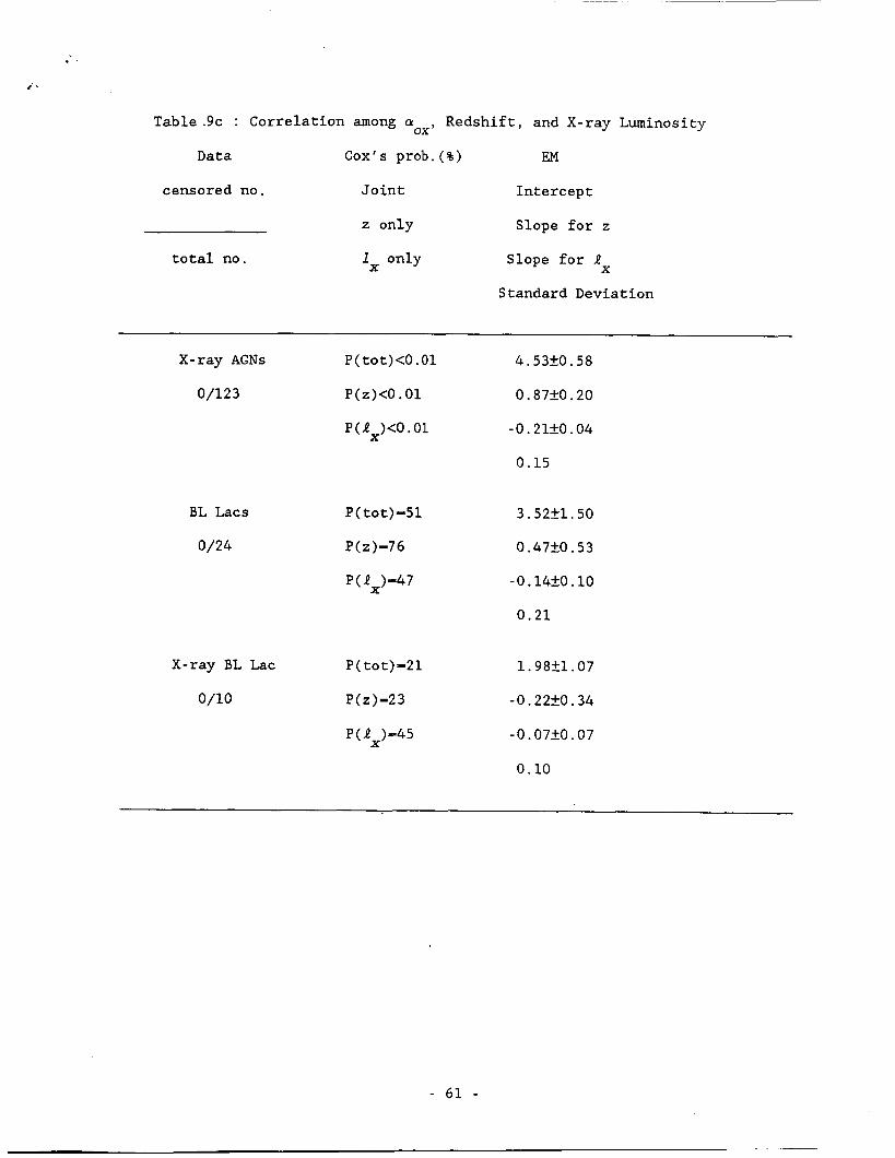
Table.9c : Correlation among a Redshift, and X-ray Luminosity ox'

Data Cox's prob. (%) EM

censored no. Joint Intercept

z only Slope for z

total no. lx only Slope for R X

Standard Deviation

X-ray AGNs P(tot)<O.Ol 4.53k0.58

0/123 P(z)<O. 01 0.87k0.20

P(RX)CO.O1 -0.21kO.04

0.15

BL Lacs

0/24

P( tot)-51

P(~)=76

P(R )-47 X

X-ray BL Lac P ( tot) -21

0/10 P(~)=23

P(R )-45 X

3.52k1.50

0.4720.53

-0.14kO.10

0.21

1.9821.07

-0.2220.34

-0.07kO.07

0.10

- 61 -

. ' :

Table 10a : Comparison of Radio Quasars and BL Lac Objects

censored no.

Property Mean and Standard Deviation

total no.

~~

Radio luminosity QSO : <log(Rr)> = 33.8820.128 ( 4 6 / 1 5 6 )

BL Lac: <log(Rr)> - 33.8120.280 ( 0 / 2 4 )

Gehan test : P = 79%

Logrank test: P - 91%

Optical luminosity QSO : <log(Ro)> - 3 1 . 2 6 2 0 . 0 6 ( 0 / 1 5 6 )

BL Lac: <log(Ro)> - 30.5420.23

Gehan test : P = 0.8%

Logrank test: P = 0.01%

( 0 / 2 4 )

X-ray luminosity QSO : <log(Rx)> - 4 5 . 6 3 2 0 . 0 6 ( 1 1 / 1 5 6 )

BL Lac: <log(Lx)> = 4 4 . 8 9 2 0 . 2 4

Gehan test : P = 0 . 6 %

Logrank test: P = 0.01%

( 0 / 2 4 )

a ro

a ox

QSO : <aro> = 0.64?0.01 ( 4 6 / 1 5 6 )

BL Lac: <a > = 0 . 6 2 2 0 . 0 2 ( 2 / 5 0 ) ro

Gehan test : P = 20%

Logrank test: P = 14%

QSO : <a > = 1 . 4 3 + 0 . 0 2 / - 0 . 0 3 ( 1 1 / 1 5 6 ) ox

( 2 / 5 0 ) BL Lac: <aox> = 1 . 4 6 2 0 . 0 3

- 62 -

Gehan test : P = 29%

Logrank t e s t : P = 25%

- 6 3 -

Table 10b : Comparison of Radio Quasars and BL Lac Objects (0.8<z<1.7)

censored no,

Property Mean and Standard Deviation

total no.

(0/57) Redshift QSO : <z> = 1.1120.03

BL Lac: <z> - 1.08?0.10 Gehan test : P - 42% Logrank test: P = 81%

Radio luminosity QSO : <log(Lr)> = 34.40k0.12 (16/57)

BL Lac: <log(R )> = 35.0420.12 r Gehan test : P - 3% Logrank test: P - 0.6%

(0/8)

Opt ica l luminosity QSO : <log(Ro)> - 31.34k0.06 (0/57)

BL Lac: <log(Ro)> = 31.3820.18

Gehan test : P = 82%

Logrank test: P - 92%

(0/8)

X-ray luminosity QSO : <log(lx)> - 45.78k0.05 (3/57)

BL Lac: <log(Rx)> - 45.92k0.17 Gehan test : P - 59% Logrank test: P - 44%

(0/8)

a ro QSO : <a ro > - 0.6020.02 (16/57)

BL Lac: <aro> - 0.69kO.03 (0/8)

- 64 -

Gehan t e s t : P = 8%

L o g r a n k t e s t : P - 3%

a ox QSO : <a > * 1.37kO.02 (3/57) ox

BL L a c : <a > - 1.39+0.08/-0.10 (0/8)

Gehan t e s t : P - 73%

L o g r a n k t e s t : P - 60%

ox

- 65 -

References

Arp, H . , Sulentic, J. W., and De Tullio, G. 1979, A?. J . 229, 489.

Ami, Y. and Tananbaum, H. 1982, Ap. J.R (Letters), 262, L17.

Ami, Y. and Tananbaum, H. 1986, Ap. J . , 305, 83.

Biermann, P., Duerbeck, H., Eckart, A., Fricke, K., Johnston, K. J.,KGhr, H.,

Liebert, J., Pauliny-Toth, I. I. K., Schleicher, H., Stockman, H.,

Strittmatter, P. A., and Witzel, A. 1981, Ap. J. (Letters), 247, L53.

Blandford, R. D. 1984 in Active Galactic Nuclei, ed. J. E. Dyson (Manchester:

Manchester Univ. Pr.) P. 281.

Blunenthal, G. R., Keel, W. C., andMiller, J. S. 1982, Ap. J., 257, 499.

Borra, E. and Corriveau, G. 1984, Ap. J., 276, 449.

Braccesi, A . , Formiggini, L., and Gabdkfi, E. 1970, Astr. Ap., 5 , 264.

Bregman, J. N. 1984, Ap. J., 276, 423.

Bregman, J. N. Glassgold, A . E. Huggins, P. J., and Kinney, A. L. 1985,

Ap. J., 291, 505.

Cash, W. and Snow, T. P. Jr. 1980, Astr. Ap. 91, L7.

Chanan, G. A., Margon, B., Helfand, D. J., Domes, R. A., and Chence, D. 1982,

A?. J. (Letters), 261, L 3 1 .

Condon, J. J., Condon, M. A . , Jouncey, D. L., Smith, M. G., Turtle, A. J., and

Wright, A. E. 1981a, Ap. J. 244, 5.

Condon , J. J. and Dressel, L. L. 1978, Ap. J., 221, 456.

Condon, J. J. and Jauncy, D. L. 1974, A. J. 79, 1220.

Condon, J. J., O'Dell, S . L., Puschell, J. J., and Stein, W. A. 1981b,

Ap. J . (Letters), 246, 624.

Cotton, W. D. 1983, Ap. J . , 271, 51.

Cruz-Gonzalez, I. and Huchra, J. P.. 1984, A. J., 89, 441.

Efron, B. 1984, J. Am. Stat. Assoc., 79, 791.

- 6 6 -

Ekers, J.. A . ( e d . ) 1969, A u s t . Phys. A s t r . S u p p l . , 7 , 1.

FilippeEko, A . V., Djorgovski, S., Spinrad, H., and Sargent, W. L. W. 1986,

A . J . , 91, 49.

Feigelson, E. D. and Berg, C. J. 1983, A p . J . , 2 6 9 , 400.

Feigelson, E. D., Bradt, H., McClintook, J., Remillard, R., Urry, C. M.,

Tapia, S., Geldzahler, B., Johnston, K., Romanishin, W., Wehinger, P. A . ,

Wyckoff, S . , Madejski, G., Schwartz, D. A . , Thorstensen, J., and Schaefer,

B. E. 1986, A p . J . , 3 0 2 , 337.

Feigelson, E. D., Isobe, T., and Kembhavi, A . 1984, A . J . , 8 9 , 1464, (Paper

1) - Feigelson ,E. D. and Nelson, P. I. 1985, A p . J . , 2 9 3 , 192.

Franceschini, A . , Gioia, I. M., and Maccacaro, T. 1986, P r e p r i n t .

Gioia, I. M., Feigelson, E. D., Maccacaro, T., Schild, R., and Zamorani, G.

1983, A p . J., 2 7 1 , 524.

Gioia, I. M., Maccacaro, T., Schild, R. E., Stocke, J. T., Leibert, J. W.

Danziger, I. J., Kunth, D., and Lub, J. 1984, A p . J . , 2 8 3 , 495.

Henriksen, M. J., Marshall, F. E., and Mushotzky, R. 1984, A p . J . , 2 8 4 , 491.

Hewitt, A . and Burbidge, G. 1980, Ap. J . S u p p l . , 4 3 , 57.

Hintzen, A . , Ulvestad, J., and Owen, F. 1983, A . J . , 8 8 , 709.

Isobe, T., Feigelson, E. D., and Nelson, P. I. 1986, A p . J . , 3 0 6 , 490.

Jenkins, C. J., Pooley, G. G., and Riley, J. M. 1977, Mem. R . A . S . , 8 4 , 61.

Johnson, H. L. 1966, Ann. Rev. A . A p . , 4 , 193.

Junkkarinen, V. T., Marscher, A . P., and Burbidge, E. M. 1982 A . J . , 8 7 , 8 4 5 .

Katgert, P., Thuan, T. X., and Windhorst, R. A . 1983, A p . J . , 2 7 5 , 1.

Kembhavi, A . 1986, IAU Symposium 119 in press.

Kembhavi, A . and Fabian, A . C. 1982, M. N. R. A . S . , 1 9 8 , 921.

Kembhavi, A . , Feigelson, E. D., and Singh, K. P. 1986, M. N. R . A . S . ,

220,51, (Paper 11).

Kb'nigl, A . 1981, A p . J., 243, 700.

K r i s s , G . A. and Canizares, C . R . 1982, A p . J.,261, 51.

K r i s s , G. A. and Canizares, C . R . 1985, A p . J., 297, 177.

Ku, W . H . - M . , Helfand, D . J . , and Lucy, L. B. 1980, Nature, 288, 323

KGhr, H . , Wi tze l , A . , Pauliny-Toth, I . I. K . , and Nauber, U . 1981,

A . A . S u p p l . , 45, 367.

Lancaster, J . F. and Quade, D . 1985, J. Am. S t a t . A S S O C . , 80, 393.

Ledden, J . E . and O ' D e l l , J . E . 1983, A p . J . , 270, 434.

Ledden, J . E. and O ' D e l l , J . E . 1985, A p . J.,,298, 630.

Maccacaro, T . and Gioia, I . M. 1983 i n

IALI Symposium 104, E a r l y Evolution of the Universe and I t s Present S t ruc ture ,

eds. G . 0 . Abell and G . Chincarini (Dordrecht: Reidel) P . 7 .

Maccacaro, T . , Gioia, I . M . , Maccagni, D . , and Stocke, J . J . 1984,

A p . J . (Letters), 2 8 4 , L23.

Maccagni, D. and Tarenghi, M . 1981, S p a c e S c i . R e v . , 30, 55.

Madejski, G . M . and Schwartz, D . A. 1983, A p . J., 275, 467.

Margon, B . , Downes, R . A . , and Chanan, G . A . 1985, A p . J. S u p p l . , 5 9 , 23.

Marscher, A. P . and Broderick, J . J . 1981, A p . J., 249, 406.

Marshall, H , L . , A m i , Y . , Braccei, A . , Huchra, J . P . , Tananbaum, H . ,

Zamorani, G., and Z i t e l l i , V . 1984, A p . J., 283, 180.

Marshall, H . L . , Zamorani, G . , Huchra, J . P . , Braccesi, A . , and Z i t e l l i , V .

1983, A p . J . , 269, 42.

Miley, G . K . and Har tsu i jker , A . P . 1978, A . A . S u p p l . , 34, 1 2 9 .

Mi l l e r , L. 1984, i n VLBI and Compact R a d i o S o u r c e s , eds. R . Fan t i , e t a l .

(Dordrecht: Re ide l ) , P . 189.

Owen, F. N . , Porcas, R . W . , and Mufson, S . L. 1978, A. J . , 83, 685.

- 68 -

Owen, F. N., Helfand, D. J., and Spangler, S. R. 1981, Ap. J. (Letters), 250,

L55 '

Owen, F. N. and Puschell, J. J. 1982, A. J., 8 7 , 595.

Owen, F. N., Spangler, S. R., and Cotton, W. D. 1980, Ap. J., 8 5 , 351.

Perley, R. A . 1982, A. J., 87, 859.

Pooley, G. G. and Henbest, S. N. 1974, M. N. R. A. S., 169, 477.

Reichert, G. A . , Mason, K. O., Thorstensen, J. R., and Bowyer, S. 1982,

Ap. J., 260, 437.

Riley, J. M. and Pooley, G. G. 1975, Mem. R. A. S., 80, 105.

Ryle, M. and Elsmore, B. 1973, M. N. R. A. S., 164, 223.

Schlosman, I., Shaham, J., and Shaviv, G. 1984, Ap. J., 287, 534.

Schmidt, M. 1968, Ap. J. 151, 393.

Schmidt, M. and Green, R. F. 1986, Ap. J., 305, 68.

Schmitt, J. H. M. M. 1985, Ap. J., 293, 178.

Schwartz, D. A . and Ku, W. H.-M. 1983, Ap. J., 266, 459.

Schwartz, D. A . , Roberts, W., Murray, S., Huchra, J., Remillard, R., Bradt,

H., McCintock, J., Tuohy, I., Buckky, D., Tapia, S . , Feigelson, E. D., and

Schmelz, J. 1985, B. A. A. S., 17, 608.

Sen, P. K. 1968, J. Am. Stat. A s s o c . , ~ ~ , 1379.

Shimmins, A . J. and Bolton, J. G. 1974, Aust. J. Phys. Astro. Suppl., 32, 1.

Shimmins, A . J., Bolton, J. G., andwall, J. V. 1975,

Aust. J. Phys. Astro. Suppl., 34, 63.

Sramek, R. A . and Weedman, D. W. 1980, Ap. J., 238,435.

Stocke, J. J., Liebert, J., Gioia, 1. M., Grrffiths, R. E., Maccacaro, T.,

Danziger, I. J., Kunth, D., and Lub, J. 1983, Ap. J., 273, 458.

Stocke, J. J., Liebert, J., Schmidt, G. D., Gioia, I. M., Maccacaro, T.,

Schild, R. E., Maccagni, D., and Arp, H. C. 1985, Ap. J., 298, 619.

- 69 -

\ <

Sulentic, J. W. 1986, A p . J., 3 0 4 , 617.

Tananbaum, H., Ami, Y., Green, R. F., Schmidt, M., and Zamorani, G. 1986,

A p . J., 3 0 5 , 57.

Tananbarn, H., Wardle, J. F. C., and Zamorani, G. 1983, A p . J., 2 6 8 , 6 0 .

Tucker, W. 1983, A p . J., 2 7 1 , 531.

Ulmer, M. P., Brown, R. L., Schwartz, D. A., Patterson, J., and Cruddace, R.

G. 1983 Ap. J. (Letters), 2 7 0 , Ll.

Ulvestad, J., Johnston, K., Perley, R., and Fomalont, E. 1981, A . J . , 8 6 ,

1010.

Ulvestad, J. S . , Johnston, K. J., and Weiler, K. W. 1983, A p . J., 2 6 6 , 18.

Ulvestad, J. S. and Wilson, A. S. 1984, A p . J., 2 8 5 , 439.

V6ron-Cetty, M. P. and VQron, P. 1983, A. A . S u p p l . , 5 3 , 219.

V6ron-Cetty, M. P.

Wardle, J. F. C., Moore, R. L., Angel, J. R. P. 1984, A p . J., 2 7 9 , 93.

Weiler, K. W. and Johnston, K. J. 1980, M. N. R . A . S., 190, 269.

Weistrop, D., Shaffer, D. B., Hintzen, P., and Romanishin, W. 1985, A p . J.,

and Vhron, P. 1984, E . S. 0. Sci. R e p . , 1, 1.

2 9 2 , 614.

Wills, D 1979, A p . J., 3 9 , 291.

Wilson, A. S., Ward, M. J., Axon, D. J., Elvis, M., and Meurs, E. J. A. 1979,

M . N . R . A . S . , 1 0 7 , 109.

Wood, K. S., Meekins, J. F., Yentis, D. J., Smathers, H. W., McNutt, D. P.,

Byram, E. T., Chubb, T. A . , and Friedman, H. 1984, A p . J . S u p p l . , 5 6 , 507.

Worrall, D. M. and Marshall, F. E. 1984 A p . J., 2 7 6 , 434.

Worrall, D. M., Puschell, J. J., Bruhweiler, F. C., Sitko, M. L., Stein, W.

A., Aller, M. F., Aller, H. D., Hodge, P. E., Rudy? R. J., Miller, H. R.,

Wisniewski, W. Z., Cordova, F. A., and Mason, K. 0. 1984, A p . J . , 2 8 4 , 5 1 2 .

Zamorani, G. 1982, A p . J. (Letters), 2 6 0 , L31.

- 70 -

Zamorani, G . 1984, i n VLBI and Compact Radio Sources, eds. R . Fanti et al.

(Dordreht: Reidelj , P . 85.

Zamorani, G . , Henry, J . P . , Maccacaro, T . , Tananbaum, H . , Soltan, A . , A m i ,

y., Liebert , J . , Stocke, J . , Str i t tmat ter , P . D . , Weymann, R . J . , Smith, M .

G . , and Condon, J . J . 1981 , A p . J. 2 4 5 , 357.

- 7 1 -

Figure Captions

Plot of the 0 . 5 - 4 . 5 keV X-ray luminosity against the 5 GHz radio

luminosity density of the radio selected quasars. The detected

points are represented by circles and the upper limits are

represented by bars in this figure and all following figures.

The solid line in this and following two figures is the

regression line log(R )-a+blog(lr) obtained by the application

of the BHK method.

Figure l(a)

X

l(b) Plot of the 0 . 5 - 4 . 5 keV X-ray luminosity against the 5 GHz radio

luminosity density of the optically selected quasars.

l(c) Plot of the 0 . 5 - 4 . 5 keV X-ray luminosity against the 5 GHz radio

luminosity density of the X-ray selected AGNs.

l(d) Plot of the 0 . 5 - 4 . 5 keV X-ray luminosity against the 5 GHz radio

luminosity density of the BL Lac objects. The radio selected BL

Lac objects are represented by circles and the X-ay selected BL

Lac objects are represented by boxes. The solid line is the

regression for the radio selected BL Lac objects and the dashed

line is the regression line for the X-ray selected BL Lacs.

Both regression lines are assumed to have a form

log(R )-a+blog(R ) and computed by a least square method. X r

Figure 2(a) Plot of the 0 . 5 - 4 . 5 keV X-ray luminosity against 2500 A optical

luminosity density of the radio selected quasars. The solid line

in this and the following two figures is the regression line

- 7 2 -

log(R )-a+blog(R ) by the EM algorithm with normal distribution. X r

2(b) Plot of the 0 . 5 - 4 . 5 keV X-ray luminosity against 2500

luminosity density of the optically selected quasars.

optical

2(c) Plot of the 0 . 5 - 4 . 5 keV X-ray luminosity against 2500 A optical

luminosity density of the X-ray selected AGNs.

2(d) Plot of the 0 . 5 - 4 . 5 keV X-ray luminosity against 2500 A optical

luminosity density of the BL Lac objects. The radio selected BL

Lac objects are represented by circles and the X-ay selected BL

Lac objects are represented by boxes. The solid line is the

regression line f o r the radio selected BL Lac objects and the

dashed line is the regression line for the X-ray selected BL

Lacs.

Figure 3(a) Plot of the 5 GHz radio luminosity density against 2500 A

optical luminosity density of the radio selected quasars. The

solid line here and in the following figures is the regression

line log(Rr)=a+blog(Ro) by the EM algorithm with the normal

distribution.

3(b) Plot of the 5 GHz radio luminosity density against 2500 A

optical luminosity density of the optically selected quasars.

The uncertainty o f the intercept coefficient is relatively large

(0.32 f 0 . 6 5 ) .

- 7 3 -

h

3(c) Plot of the 5 GHz radio luminosity density against 2500 A

optical luminosity density of the X-ray selected AGNs.

uncertainty of the intercept coefficient is relatively large ( -

34.5 * 12.0).

The

3(d) Plot of the 5 GHz radio luminosity density against 2500 A

optical luminosity density of the BL Lac objects. The radio

selected BL Lac objects are represented by circles and the X-ay

selected BL Lac objects are represented by boxes. The solid line

is the regression line for the radio selected BL Lac objects and

the dashed line is the regression line for the X-ray selected BL

Lacs.

Figure 4(a) Plot of the aox against the a

The solid line is the regression line a =a+ba

application the BHK method.

following four figures represent lower limits.

of the radio selected quasars. ro

by the ox ro

The bars in this figure and

4(b) Plot of the aOX against the a

quasars. Because of the large uncertainty for the intercept here

and below, we do not fit a regression line.

of the optically selected ro

4(c) Plot of the aox against the a of the X-ray AGNs. ro

4(d) Plot of the aOX against the a

selected BL Lac objects are represented by circles and the X-ay

selected BL Lac objects are represented by boxes. The solid line

of the BL Lac objects. The radio 10

- 14 -

is the regression line for the radio selected BL Lac objects and

the dashed line is the regression line for the X-ray selected BL

Lac objects.

4(e) Plot of the aox against the a

The arrow in this figure represents an upper limit.

of the compact radio sources ro

- 7 5 -

___

Authors' Addresses

Eric D. Feigelson and Takashi Isobe

Department of Astronomy, The Pennsylvania State University, University

Park, PA 16802.

Kulinder P. Singh and Ajit Rembhavi

Tata Institute of Fundamental Research, Homi Bhabha Road, Bombay 400 005,

India.

- 7 6 -

Fig . 1

Fig. 2

I I I I I I I I I I I I I I I I I I I I

Fig. 3

Fig. 4

Fig. 4

x 0

1.8 1.6 \

3 k \

1.4 f- \ i L \

1.21 c \- Lot

0.8 1 c aj -0.1 0.1 0.3 0.5 0.7 09 1.1