nature of poverty and identification of poor in small …
TRANSCRIPT

NATURE OF POVERTY AND IDENTIFICATION
OF POOR IN SMALL AND MEDIUM TOWNS
Sponsored by
Ministry of Housing and Urban Poverty Alleviation
And
Planning Commission
INSTITUTE FOR HUMAN DEVELOPMENT
NIDM Building, IIPA Campus, I.P. Estate
Mahatma Gandhi Marg, New Delhi-110002
Tel: 23358166, 23321610 / Fax: 23765410
E-mail: [email protected], Website: www.ihdindia.org
May 2012

NATURE OF POVERTY AND IDENTIFICATION
OF POOR IN SMALL AND MEDIUM TOWNS
Sponsored by
Ministry of Housing and Urban Poverty Alleviation
And
Planning Commission
Project Director
Alakh N. Sharma
Principal Researcher
Nandita Gupta
INSTITUTE FOR HUMAN DEVELOPMENT
NIDM Building, IIPA Campus, I.P. Estate
Mahatma Gandhi Marg, New Delhi-110002
Tel: 23358166, 23321610 / Fax: 23765410
E-mail: [email protected], Website: www.ihdindia.org
May 2012

PREFACE
In recent years urban poverty has acquired much attention thanks to the increasing pace of urbanisation in the country and the movement of large masses of rural poor to urban centres. However, the problems of poverty and livelihoods in small and medium towns have hardly been systematically studied and research so far has largely concentrated on larger cities and metropolises.
In this context, IHD was given the task of conducting the study on "Nature of Poverty and Identification of Poor in Small and Medium Towns" by the Steering Group on Identification of Urban Poor chaired by Prof. S.R. Hashim.
We are thankful to Planning Commission and the Ministry of Housing and Urban Poverty Alleviation and in particular Dr. P.K. Mohanty for sponsoring this study. We express our particular thanks to Prof. S.R. Hashim for his inputs and guidance.
We received very rich comments from all the experts and members of the Steering Group on the presentation of the draft report at the Planning Commission. We are very thankful for their insightful feedback.
The field work for this study, conducted in six towns, each from a different state, was a challenging one and it would not have been possible without the support of Prof. R.S. Ghuman in Mansa, Dr. Venkatnarayan Motkuri in Jangaon, Dr. Vinay Das in Madhubani, Dr. Chaya Degaonkar in Bidar, and Mr. Ashwini Kumar in Pakur.
The difficult task of field work was conducted by a dedicated team of field investigators. We express our deepest thanks to them. List of all investigators are in Annexure 6.
This study was further enriched by colleagues at the institute, and we are thankful to them for their inputs and help at various stages of the work. We particularly thank Dr. Rajesh Shukla for his valuable inputs and Dr. Sunil Mishra for leading the data processing work. We thank Ms. Shivani Satija, Mr. Jayprakash Sharma and Ms. Ruchika Khanna for their enthusiasm and support in conducting fieldwork in various towns.
I record my deep sense of appreciation for Ms. Nandita Gupta, the principal researcher of this study for the good work. She not only led the field work but also individually authored the report.
Alakh N. Sharma
Director, Institute for Human Development

Contents
Executive Summary ......................................................................................................... i-xi
1. INTRODUCTION, AIMS, METHODS AND CHARACTERISTICS OF SMTS STUDIED ...................................................................................................1
1.1 Objectives of the study.............................................................................................3
1.2 Research questions ...................................................................................................4
1.3 Methodology ............................................................................................................4
1.4 Limitations of the study ...........................................................................................8
1.5 Characteristics of selected SMTs and their districts ................................................9
2. NATURE OF POVERTY IN SMALL AND MEDIUM TOWNS .... ....................15
2.1 Residential Characteristics of Settlements and Households ..................................15
2.2 Cooking Fuel and Assets .......................................................................................27
2.3 Social Characteristics .............................................................................................30
2.4 Education of household, Transport and Healthcare services .................................34
2.5 Occupational Profile in SMTs ...............................................................................36
3. INCOME AND EXPENDITURE IN SMTS ...........................................................47
4. POSSIBLE INDICATORS FOR DEVELOPING IDENTIFICATIO N CRITERIA.......................................................................................................................50
4.1 Material of Roof ....................................................................................................52
4.2 Material of Floor ...................................................................................................53
4.3 Material of Wall ....................................................................................................54
4.4 Main Source of Lighting .......................................................................................55
4.5 Cooking Area of households .................................................................................56
4.6 Drinking Water Source ..........................................................................................57
4.7 Main Fuel used for Cooking ..................................................................................58
4.8 Assets Categories ..................................................................................................59
4.9 Religion .................................................................................................................60
4.10 Caste Groups .......................................................................................................61
4.11 Education Level ...................................................................................................62
4.12 Female Headed Households ................................................................................63
4.13 Households with Disabled Person .......................................................................64
4.14 Activity Status of Households .............................................................................65
4.15 Occupation of Household ....................................................................................66
5. PUBLIC DISTRIBUTION AND PRESENT TARGETING FOR WE LFARE BENEFITS IN SMTS ................................................................................................68
6. CONCLUDING SUMMARY ...................................................................................70
7. ANNEXURES ............................................................................................................72
Annexure 1: Questionnaire .........................................................................................72
Annexure 2: FGD and PRE Guidelines .......................................................................73
Annexure 3: Methodology for Obtaining Income Data ..............................................77
Annexure 4: Methodology for Obtaining Expenditure Data .......................................77
Annexure 5: Tables .....................................................................................................79
Annexure 6: List of Supervisors & Field Investigators .............................................106

i
NATURE OF POVERTY AND IDENTIFICATION OF POOR IN SMALL AND MEDIUM TOWNS
Executive Summary
1. Introduction
• This study aims at understanding the nature of poverty in small and medium towns
(SMT) in India, focusing on occupational, environmental and social vulnerabilities of
households.
The study also aims to identify simple and visible indicators which are best related to
household poverty and deprivation to bring about the creation of more universally
applicable indicators for a broader range of urban settlements.
• Six small and medium towns of various types from classes A, B and C have been
selected from different States on the basis of factors such as size, nature of economic
activities, employment pattern and locations. The selected towns in descending order
of population are Parbhani (Maharashtra), Bidar (Karnataka), Mansa (Punjab),
Madhubani (Bihar), Jangaon (Andhra Pradesh) and Pakur (Jharkhand).
• Quantitative as well as qualitative tools - Questionnaires, Focus Group Discussions
(FGD) and Poverty Ranking Exercises (PRE) have been employed in the study.
• A total of 2,168 households were covered in the questionnaire survey and the sample
was drawn from only poor localities. The survey covered approximately 1.0 per cent
to 2.7 per cent of the respective town populations as per the Census of India 2001.
The survey was carried out in a total of 59 settlements through 44 FGDs and PREs.
2. Income and Expenditure in SMTs
• Across towns, about 60 per cent of the household expenditure was on food items, 24
per cent on non-food items and 16.3 per cent on health and education.
• Household expenditure on food items was the highest in Mansa (71.6 per cent), lower
in Bidar (58.3 per cent) and the least in Jangaon (46.3per cent), Expenditure on food
items was between 59 per cent and 64 per cent in other SMTs.
ii
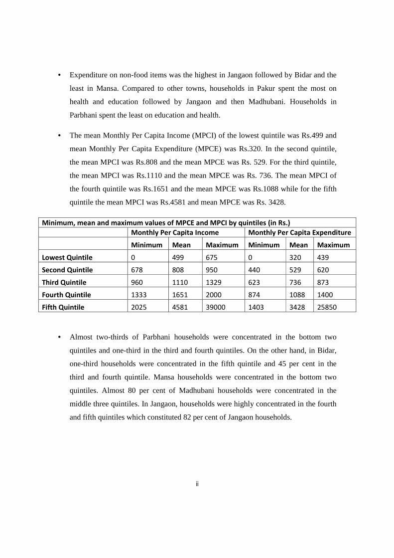
• Expenditure on non-food items was the highest in Jangaon followed by Bidar and the
least in Mansa. Compared to other towns, households in Pakur spent the most on
health and education followed by Jangaon and then Madhubani. Households in
Parbhani spent the least on education and health.
• The mean Monthly Per Capita Income (MPCI) of the lowest quintile was Rs.499 and
mean Monthly Per Capita Expenditure (MPCE) was Rs.320. In the second quintile,
the mean MPCI was Rs.808 and the mean MPCE was Rs. 529. For the third quintile,
the mean MPCI was Rs.1110 and the mean MPCE was Rs. 736. The mean MPCI of
the fourth quintile was Rs.1651 and the mean MPCE was Rs.1088 while for the fifth
quintile the mean MPCI was Rs.4581 and mean MPCE was Rs. 3428.
Minimum, mean and maximum values of MPCE and MPCI by quintiles (in Rs.)
Monthly Per Capita Income Monthly Per Capita Expenditure
Minimum Mean Maximum Minimum Mean Maximum
Lowest Quintile 0 499 675 0 320 439
Second Quintile 678 808 950 440 529 620
Third Quintile 960 1110 1329 623 736 873
Fourth Quintile 1333 1651 2000 874 1088 1400
Fifth Quintile 2025 4581 39000 1403 3428 25850
• Almost two-thirds of Parbhani households were concentrated in the bottom two
quintiles and one-third in the third and fourth quintiles. On the other hand, in Bidar,
one-third households were concentrated in the fifth quintile and 45 per cent in the
third and fourth quintile. Mansa households were concentrated in the bottom two
quintiles. Almost 80 per cent of Madhubani households were concentrated in the
middle three quintiles. In Jangaon, households were highly concentrated in the fourth
and fifth quintiles which constituted 82 per cent of Jangaon households.

iii
3. Housing and Housing Related Vulnerabilities and Indicators
• The state of housing in the selected SMTs was less precarious compared to larger
cities. This is largely due to (1) presence of tenure security - as households are largely
living on ancestral or own property. (2) Land prices and density have not increased
dramatically and (3) lack of or low density of infrastructure such as railway tracks
and big drains which can lead to a precarious state of housing.
• Overall, about one-third of house roofs were pucca (cement, bricks), three-fifths were
semi-pucca (tiled, tin sheets, asbestos sheets wooden) and almost one-tenth were
kuccha (thatch grass, tarpaulin). Presence of kuccha roofs may be used as inclusion
criteria, but presence of pucca roofs may not be used as exclusion criteria, as
exclusion errors are likely to be large.
• About 43 per cent houses had kuccha flooring (earthen and semi-earthen), the rest had
more or less pucca flooring (bricks, cement, chips/tiles, marble/stone). Use of
flooring material as inclusion and exclusion criteria is likely to entail large errors.
• Overall, one-fourth households had kuccha walls (straw, wood, bamboo, tin, wood),
one-fifth households had semi-pucca walls and almost 57 per cent households had
pucca walls (tiled, bricks and concrete). Most kuccha walls could be used for
inclusion, with some errors; however exclusion of pucca walls would entail large
errors.
• The continuum of housing ranged from kuccha, with mud housing and tarpaulin roofs
to pucca, using bricks, cement, beams etc. As reported in PREs, those living in
kuccha houses were the poorest of the poor while those living in pucca houses were
placed among the relatively-better off amongst the poor. Jangaon and Bidar were an
exception as the poorest of the poor were living in pucca houses which were publicly
provided. In case of semi pucca housing, there was no clear perception-based
consensus regarding the deprivation level of these households in the community.
iv
• Therefore, the poorest of poor could be easily identified using housing related criteria
and the relatively better-off could also be identified with some errors. The middle
section was large and the middle brackets among the poor were difficult to
distinguish between using only housing related criteria. Therefore, to segregate the
large middle bracket, other indicators or a combination of other indicators would be
required.
• Access to private sources of water was largely considered as an indicator of being
better-off by communities; however the use of private sources of water as exclusion
criteria may entail large errors. The general notion of piped water supply being an
indicator of being better-off within the poor was not supported by communities as
access to piped water supply was largely dependent on the town’s coverage of water
network.
• A total of 83.2 per cent households reported using electricity as the main source of
lighting - this was near universal (around 98 per cent ) in Parbhani, Bidar and
Jangaon, and lowest at 30 per cent in Madhubani. Lack of electricity in the
households could be used to identify the poorest of poor households, especially in
towns with near universal electrification.
• Household criteria based on public goods and town connectivity such as electricity in
the household, water supply and piped water showed little difference across
expenditure quintiles. These services were definitely better available to the richer
sections, but within the poorer groups they were equally difficult to access for even
the relatively well-off.
• In most communities, households with separate kitchens were perceived as better-off
but in many cases the very poor also had separate kitchen spaces. Many Jangaon
households, including the very poor had been provided housing by the government
which had separate spaces for kitchens. Overall, those with separate kitchens could be
excluded, but this would not be without errors. However, including those with no
separate kitchens is likely to entail large errors.

v
4. Assets and Cooking Fuel
• White goods such as refrigerators and air-coolers were being used by many poor
households. Even in the lowest monthly per capita expenditure (MPCE) quintile,
about 10 per cent of the households had a refrigerator or air-cooler.
• Assets such as four wheelers, heavy vehicles, air-conditioners, computers, washing
machines, heaters and geysers were being used by very few and relatively better off
households. These could be used for exclusion, but they are also likely to entail very
small exclusion errors.
• Household with bulbs/ tube lights as the only electric gadgets could be identified as
the poorest of poor.
• Poor cooking fuels were concentrated in the first three quintiles but a considerable
proportion was also present in the fourth and fifth quintiles. However, those using
LPG were highly concentrated in the top two quintiles and only 8.5 per cent were in
the lowest quintile, thus making the presence of LPG a better exclusion criteria rather
than use of poorer fuels being an inclusion criterion. Still, such exclusion criteria
could not be used without large errors in areas where government distribution and
subsidies on stoves and LPG have been implemented.
5. Social Vulnerabilities
• A total of 8.3 per cent households reported a disabled person in the household. These
households were highly concentrated in the lowest two quintiles and there was a clear
trend of such households decreasing with increasing per capita income and
expenditure. There is a clear case for giving greater inclusionary weight to
households with a disabled member.

vi
• Female headed households and single women were repeatedly reported as the most
vulnerable and poor in all towns and settlements. Twelve per cent of households were
reported as female headed. Female headed households were highest in the lowest
quintile. Even though female headed households did not show a consistent decline
with increasing MPCI and MPCE quintiles, communities in all towns reported female
headed households to be more deprived and vulnerable and therefore could be
considered for greater inclusionary weight.
• Leper households and households with only elderly were reported to be very poor in
all communities and could be automatically included with little error within poor
localities.
• With regard to the highest level of education of households, there was a decreasing
trend in households with increasing income and expenditure till middle school
education. This trend reversed from secondary school onwards, where households
started increasing with increasing income and expenditure. However, the level of
education was not seen as an indicator of poverty or as a real opportunity for
economic mobility by communities. Using the level of education as a criteria could
also be a case of perverse incentivizing. Following from the above arguments, the
level of education may not be used as exclusion criteria, however households with no
literate person could be considered for higher inclusionary weight.
• Sikhs and Buddhists (concentrated in Mansa and Parbhani respectively) showed a
clear declining trend with increasing MPCE and MPCI quintiles; Muslims showed a
declining trend in case of MPCI quintiles but not MPCE quintiles. Hindus showed a
slight increasing trend with increasing quintiles. Christians showed an increasing
trend with both MPCE and MPCI quintiles. However, no clear conclusion could be
drawn regarding inclusion, exclusion or weighting.

vii
• Scheduled Castes (SC) and Scheduled Tribes (ST) showed a decreasing trend with
increasing quintiles. Seventy per cent of both SCs and STs were in the bottom three
quintiles, whereas more than 70 per cent of General Category and Other Backward
Castes were in the top three quintiles. As such, SCs and STs should be considered for
greater inclusionary weight.
6. Occupational Vulnerabilities
• Overall, 36 per cent of the total earning individuals were casual wage labour,
followed by own account workers who were 25 per cent, followed by regular wage/
salaried which were 22 per cent. A total of 5.8 per cent were engaged in piece rate
work, 4.2 per cent were pensioners, 2.5 per cent were self-employed employers and
1.9 per cent were beggars.
• Households, whose main working member was self-employed employer, were
concentrated in the top two quintiles. Own account workers were distributed
uniformly across quintiles. Regular wage and salaried workers were slightly more
concentrated in the higher quintiles but had a sizeable proportion in the bottom
quintiles. Overall, self-employed employers were concentrated in the top two
quintiles, beggars in the bottom two and there was a clear trend in case of casual
wagers being poorer.
• About 1.5 per cent of girls and 3 per cent of boys in the age group of 6-14 years
reported working outside the house and 1 per cent of both boys and girls in this age
group were working as unpaid family labour.
• Irregular and insecure employment and seasonal non-availability of work were
reported as major issues in all towns. Unemployment was also reported as a major
concern among youth and many with higher education reported feeling
‘inappropriately employed’ in casual work.

viii
• Overall, the mean income of the self-employed employer was highest at Rs. 7,243 per
month, followed by regular wage/salaried workers whose mean income was Rs. 4,393
per month, followed by own account workers at 3,395 per month and finally casual
wage labour who were earning Rs.3,055 per month. The lowest monthly incomes
were of household-based piece rate workers who were earning an average of Rs.1,660
per month.
• The highest incomes were being earned by government teachers and doctors followed
by security forces and other middle level government staff. Other higher-notch
professionals such as doctors and engineers were monthly earning Rs.12,700,
followed by government clerical staff, small business owners and contractors.
• Workers earning between Rs.4,000 – 5,000 per month were auto drivers, masons,
private drivers, shop owners, lower level administrative staff (privately employed),
nurses, ward boys, salesman, chit fund brokers, and government sweepers.
• Workers earning between Rs.2500 – 4000 monthly were construction labour, brick
kiln labour, head load workers, other factory and casual labour, rickshaw pullers and
cart pullers, welders, carpenters, plumbers, hotel waiters, painters, hawkers and
vendors, small household manufacturing unit owners, small shop owners (of
tea/beedii/pan), repair mechanics, traditional artisans (weavers, bidri workers, kite
makers, goldsmiths), security guards, priests and barbers.
• Workers such as construction labour, agricultural labour, cobblers, headload workers,
rickshaw pullers, cart pullers, hotel waiters, rag pickers, scrap workers, private
sweepers, domestic workers, and helpers showed a clear decline with increasing
MPCI quintiles.
• On the other hand, workers such as welders, carpenters, polishers, fabricators,
electricians, higher rung professionals such as doctors and engineers, small business
owners, contractors, raj mistri, masons and government employees showed an
increase with increasing MPCI quintiles.

ix
• Households with government teachers and doctors had the highest MPCI of Rs.9,425
and the highest MPCE of Rs. 3,493. They were followed by households with
engineers and doctors, those in security forces, other middle level government
employment. Private teachers, small business owners, construction and other
supervisors, government peons and drivers, privately employed lower level
administrative staff and government sweepers had an MPCI of more than Rs.2,500
and MPCE of more than Rs. 1,700.
• Households with welders, carpenters, plumbers, electricians, saw mill labour,
traditional artisans, hawkers and vendors, tailors, auto drivers, other drivers, mistris,
masons, shop owners, small household manufacturers, tea, pan and beedi shop
owners, salesmen, repair mechanics, nurses, ward boys, shop assistants, priests,
barbers had a MPCI between Rs. 1,500 and Rs.2,500 and MPCE between Rs.1,000
and Rs.2,000.
• Cobblers had the lowest MPCI of Rs. 852, followed by beggars at Rs. 1,004 and rag
pickers at Rs. 1,096. Households with cobblers, beggars, rag pickers, unskilled casual
wage labourers and rickshaw pullers could be automatically included with little error.
7. Present Targeting for Welfare Benefits in Towns
• Though public distribution of food items and kerosene to households was taking place
in all SMTs, about 21 per cent of the sample households reported not having any
Above Poverty Line (APL), Below Poverty Line (BPL), Antoydaya or other cards.
This percentage was very high in Parbhani and Pakur- almost 40 per cent of the
households and the lowest in Mansa where almost one-tenth of households did not
have any card.
• In relation with MPCE quintiles, there was an increase in APL cards with increase in
quintiles however 12.5 per cent, 14.7 per cent and 16.8 per cent of the lowest, second
and third quintiles respectively had APL cards. A greater percentage-20.4 per cent, 25
per cent and 22.4 per cent of the first, second and third quintiles had no cards. Of all

x
quintiles, the fifth quintile had the lowest percentage of households which did not
have a card.
• Households with a BPL/Antoydaya or other card were more or less uniform across
the quintiles, but were slightly higher in the first and fifth quintiles. The trends were
similar in case of MPCI quintiles.
• It is clear from the results that present targeting for distribution of welfare benefits
has inclusion and exclusion errors, as 20 percent of the lowest quintile did not have
any card and 25 per cent of the second quintile did not have any card. Similarly 12.5
per cent of lowest quintile households had APL cards, and 14 per cent of second
quintile households had APL cards.
8. Conclusion
• Present targeting of poor for public distribution of food in SMTs was poor. Of the
indicators assessed for their relation with per capita expenditure, no indicator was
universal or extremely sensitive for identifying poor.
• Household criteria based on public goods and town connectivity such as electricity in
the household, water supply and piped water showed little difference across
expenditure quintiles. These services were definitely better available to the richer
sections, but within the poorer groups, they were equally difficult to access for even
the relatively – well off.
• Places with high disbursement of government benefits had hidden poverty not
captured by criteria such as housing, fuels, assets etc. Dependency on such benefits
was also widespread. The danger of excluding poor and vulnerable households is very
high, particularly in some states and regions, making it imperative to account for
government benefits in these areas and states.
• Some issues with present state-specific criteria and targeting were raised by
municipality staff and residents; such as where the possession of a cell phone was
reported as being used as exclusion criteria. Similarly, where brick housing was being

xi
excluded from benefits, households complained that even though their walls were
made of bricks, they had only been stacked and had no mortar, making their housing
vulnerable. This merits careful surveying and incorporating nuances of building
materials and layout in order to capture housing and other vulnerabilities.
• With little inclusion error, poor settlements in towns such as Madhubani and Pakur as
a whole can be identified as poor due to the homogenous nature of settlements; this
would not be possible in other towns. In Jangaon, for instance there are settlements
where middle income households, rich households and very poor are living together,
mainly due to soaring demand for land and gentrification due to availability of basic
services in these settlements.
• When compared with bigger cities and towns, it is not surprising that issues related to
precariousness of the state of housing and tenure are muted in SMTs. However, the
two bigger SMTs show a greater degree of precariousness and an increasing tendency
towards precariousness.
• Dominance of regional materials, regional fuels and regional practices is high in
SMTs – for example, use of stone and khapra and local fuels. Regional elements may
not be as dominant in bigger cities and towns.
• It was also noted that the value of materials changed with the passage of time and
availability of newer materials – for example, kaveli/ khapra were the only option
after thatched roofs in Pakur. These tiles are now considered in the more expensive
range due to availability of other cheaper materials such as brick, tin and asbestos.
• In case of the six SMTs, there was also an issue in valuation of indicators due to
regional and local supplies and subsidies– for example, coal may not be considered a
cheap fuel, but is very cheaply available in Pakur (Jharkhand) and is being used by a
large majority of the poor. This makes it important to understand the relative values
of housing materials and other indicators in a regional context before using them for
purposes of inclusion, exclusion or greater weight.

xii
• Issues related with hidden poverty due to disbursement of benefits, use of regional
fuels and construction material, different valuations of materials across time and
regions indicate the need for a regional approach to identification of poor. It becomes
imperative that some regional criteria should be included in the identification process
to be able to address issues of relative and absolute poverty across towns and states.

1
NATURE OF POVERTY AND IDENTIFICATION OF POOR IN SMALL AND MEDIUM TOWNS
I.
1. INTRODUCTION: AIMS, METHODS AND CHARACTERISTICS OF SMTS STUDIED
While India is facing an urbanization challenge- the challenge is most acute in small and
medium towns, where the share of urban population is lower, and growth is slower
compared to big urban centres (Report on Indian Urban Infrastructure and Services,
20111). Smaller towns are also seen as being more vulnerable due to their less developed
economic foundation, governing capacities and resources, weak access to public services
and poor planning. The heterogeneous nature of urban centres is highlighted by Kundu
and Sarangi (20052) in terms of poverty characteristics, where they point out that while
the million plus cities and medium category towns (50,000 – 100,000 population) report
poverty levels of around 14 per cent and 20 per cent respectively in 1999 – 2000 (55th
Round); the corresponding figure for smaller towns (50,000 or less population) is as high
as 24 per cent. Calculations based on the 1993 – 94 data (50th Round) show metropolises
as having the lowest poverty at 23 per cent and medium cities / towns and small towns
with poverty figures of 32 per cent and 36 per cent respectively. While the metropolitan
cities have some similarities and are linked to the global economy, the small and medium
towns are linked to the local economies, and hence are more diverse in economic
structures and governance capabilities than the metropolitan cities. Further, the
economies of small and medium towns are more closely linked with the state’s economy
and hence also the nature of poverty.
Even though economic reforms have brought about some investment through government
programmes and creation of Special Economic Zones (SEZs) around smaller urban
centres, these economies are still dominated by a significantly large agricultural
economy.
1 Report on Indian Urban Infrastructure and Services (2011),http://cistup.iisc.ernet.in/Urban%20Mobility%208th%20March%202012/urban%20india%20infrastructure%20report.pdf 2 Kundu, A. and Sarangi, N. (2005) 'Issue of Urban Exclusion' Economic and Political Weekly 40 (33) p. 3642 -3646
2
According to Sharma (April 20093), more than 180 million (which is more than half of
the urban population according to the 2001 Census) live in small and medium towns.
There is little urban literature which focuses on the subject; usually the emphasis tends to
be on the big urban towns and metropolitan cities.
In big cities and metropolises, the main issues for the economically backward are to do
with housing, the distance between work and residence and access to education and
health both in terms of cost of getting to those services and the cost of services. The
metropolitan cities offer greater work opportunities and those having a foothold in the
city need guaranteed access to shelter, education and healthcare. In smaller cities,
however, housing and commuting may not seem like the most pressing issue. According
to Sharma (April 2009), slums are a major feature of smaller towns-almost one-fourth of
the population live in slums. Economic development, a strong financial base, decent
public services (waste management in particular), employment opportunities, education,
health care facilities and governance capabilities seem to be more important than shelter
in the small and medium towns.
With respect to the identification of urban poor a country-wide identification process has
not been undertaken so far. Beneficiary targeting has so far been done on the basis of
state-specific criteria. Findings from reports such as the 2008 Pranob Sen Committee on
Slum Statistics and Census has been useful for settlement targeting but not intended for
targeting poor and vulnerable households or individuals.
Identification of Below Poverty Line (BPL) households in India for distribution of
welfare benefits was first initiated in 1992. Countrywide identification has been
conducted three times since; but in rural areas. The identification process in 1992 used
household income based on all-India income poverty line as the criteria for identification
of BPL households. In the second survey conducted in 1997, a two-step approach was
followed, of first excluding the visibly non-poor and then selecting households on the
3 http://infochangeindia.org/Urban-India/Cityscapes/Slumdogs-and-small-towns.html

3
basis of expenditure calculated over 30 days and other demographic characteristics. In
2002, a third process for identifying those below poverty line was undertaken using 13
indicators which were scored and households selected based on a cut-off.
Issues faced in identification processes have been widely documented in case of
aforementioned surveys including efforts at capturing multidimensional aspects of
poverty. At large they have been an improvement over their predecessors, but have
nevertheless been criticized for methodological issues (indicators chosen, weighting etc.),
implementation issues (nepotism, misplaced incentivisation of panchayats and other
structures) and other issues relating to arbitrary cut-offs at state and national levels.
The heterogeneity of Indian urbanization in terms of human and economic development,
geographical and lifestyle differences and others created by differential regional
development and state policies are a challenge to creating a sound methodology for
identification fitted to implementation and resource constraints.
Moreover, literature and statistics on urban populations and poverty which can inform
identification process design and information on small and medium towns (SMTs) is very
limited. Given the paucity of information and the heterogeneity of urban area and
regions, this study aims to fill some of the information gaps and provide an indicative
understanding with respect to poverty in SMTs.
1.1 Objectives of the study
This study aims at understanding the nature of poverty in small and medium towns in
India, focusing on occupational, environmental, social vulnerabilities of households and
access to basic services.
The study also aims to identify simple and visible indicators which are best related to
household poverty and deprivation to inform the creation of more universally applicable
indicators for a broader range of urban settlements.

4
Research Questions
The study aims to address the following questions:
1. What is the nature of social, occupational, and residential deprivations faced by the poor in SMTs?
2. To what extent are basic services available to the poor and what kind of access do they have to them?
3. What can be the verifiable indicators which may be used to identify poor in these SMTs?
1.3 Methodology
1.3.1 Coverage and Selection of Towns
As per the 74th Constitutional Amendment (CAA), urban centres are classified into
four classes- M, A, B and C for the purpose of urban governance and financial
allocations. The class M cities have Municipal Corporations (population of 3 lakhs
and above), class A are cities with Municipalities (population of 1 to 3 lakhs); class B
consists of towns with Nagar Panchayats (population of 50,000 to 1 lakh) and class C
are towns with population less than 50,000.
Six small and medium towns of various types from town classes A, B and C have
been selected from different states on the basis of factors such as size, nature of
economic activities, employment pattern and locations. The selected towns in
descending order of population are Parbhani (Maharashtra), Bidar (Karnataka),
Mansa (Punjab), Madhubani (Bihar), Jangaon (Andhra Pradesh) and Pakur
(Jharkhand).

5
Table 1: Selection of towns Name of town State Population
(2001 census) Class A towns (Population between 1 and 3 lakh)
Parbhani Maharashtra 2,59,170
Bidar Karnataka 1,72,877
Class B towns (Population between 50,000 and 1 lakh)
Mansa Punjab 72,627 Madhubani Bihar 66,340
Class C towns (Population less than 50,000)
Jangaon Andhra Pradesh 43,996 Pakur Jharkhand 36,029
1.3.2 Data Collection Tools
Both qualitative and quantitative data collection tools have been employed in the
study. They are:
• Questionnaire: Household level information on housing conditions,
expenditures, migration to and from the town, tenure, identity proofs, availability
of government schemes, access to basic services, asset ownership and perceptions
were collected. Details regarding the demographic profile, occupational activity
and educational profile, residential status and incomes were collected for
individuals. Income data has was collected for individuals involved in both
primary and secondary activities. Expenditure data was collected for households.
Both income and expenditure data have been analysed to provide only an
indicative assessment and not an exact estimation.
The questionnaire can be viewed in Annexure 1 and methodology used for collecting income and expenditure data is in Annexure 3.
• Focus Group Discussion (FGD): FGDs were conducted in mixed groups of 10 to
20 members in selected poor settlements. Through FGDs, information was
collected on community and environmental assets and resources, views and
perceptions on basic services, tenure, infrastructure, housing conditions,

6
education, public distribution system (PDS), seasonality and other community,
household and individual issues.
• Poverty Ranking Exercise (PRE): PREs were conducted following each FGD
with the same participants. Participants were asked if it was possible to divide
their communities into a continuum of the poorest of poor and the least poor and
if there were some verifiable characteristics of these different divisions.
Participants classified their own communities into divisions up to 5 and gave both
verifiable and non-verifiable characteristics for each division they proposed. FGD
and PRE guidelines are in Annexure 2.
1.3.3 Sample Selection
A total of 2,168 households were covered in the questionnaire survey and the
sample was only drawn from poor localities. The survey covered approximately 1
per cent to 2.7 per cent of the town population as per the Census of India 2001.
The survey was conducted in a total of 59 settlements through 44 FGDs and
PREs.
• Consultations with Municipality staff, Rickshaw pullers and other town
residents: Consultations were held with municipality staff to identify pockets of
poor residents on a ward map of the town. Different areas were identified on the
basis of religion, caste and occupation of settlers, period of existence of
settlements, ownership status of land and migrant settlements and other local
factors. The history of town formation and development, extension, growth of
industries, migration, and connections with other cities were probed during these
consultations. Informal conversations with rickshaw pullers, hawkers and vendors
helped in understanding the salient differences among the various kinds of
settlements and their histories.
• Town Transect and Settlement Mapping: A transect walk of all settlements
listed during municipality and other consultations was carried out. The

7
understanding gained from this exercise was used in purposive sampling of
settlements.
Questionnaires:
Number of household questionnaires to be conducted per settlement were pre-fixed
within a range of 30 - 40 considering the homogeneity of settlements in SMTs.
Following from this, the number of sample settlements per town category was fixed.
Sample of 13 to17 settlements could be taken in class A towns, 8 to10 in class B towns
and 6 to 7 in class C towns.
• Selection of wards: Wards were first stratified on the basis of SC/ST/ BPL
population as per the Census 2001 and where available Census 2011. Wards were
Table 2: Sample Selection in SMTs
Name of town
State Population
Questionnaires per urban centre
Sample Population (% of Total Population)
FGDs per urban centre
Class A towns (Population between 1 and 3 lakh)
Parbhani Maharashtra
2,59,170 545 2795 (1.08%)
9
Bidar Karnataka 1,72,877 544 2291 (1.33%)
9
Class B towns (Population between 50,000 and 1 lakh)
Mansa Punjab 72,627 314 1567 (2.16%)
7
Madhubani Bihar 66,340 312 1805 (2.72%)
7
Class C towns (Population less than 50,000)
Jangaon Andhra Pradesh
43,996 242 747 (1.70%)
6
Pakur Jharkhand 36,029 210 908 (2.52%)
6
Total 2168 10113 44

8
chosen from each list of stratified wards, on the basis of inputs gathered from
consultations with municipal staff and other sources and on the basis of town
transect in order to capture environmental and social differences.
• Selection of settlements: The number of settlements to be selected from each
ward was based on their respective population as per census data. The number of
settlements to be selected was also pre-fixed within the above mentioned range
depending on the class of the town. For each town a population mark was fixed
for selection of settlements from wards, if the selected wards’ population was less
than the population mark, one settlement was chosen; two settlements were
chosen if the wards’ population was more. Selection of the designated number of
settlements from each ward was done purposively, and aimed at capturing
environmental and socio-economic differences.
Focus Group Discussions and Poverty Ranking Exercise:
FGDs and PREs were conducted in 60-70 per cent of the settlements sampled for
questionnaire based data collection. The selection of settlements for conducting FGD and
PRE was done purposively from the pool. The selection was an effort to capture
qualitative data from the various kinds of settlements.
1.4 Limitations of the Study
This study does not include the houseless poor in SMTs.
Secondly, housing conditions, assets etc. are affected by government schemes and
benefits. How particular households have been influenced by government schemes and
benefits has not been covered by the survey.
The analysis in this report is based on the primary activity status of household members
and does not take into account the multiple activities and employment poor households
engage in.

9
The sample of the study is drawn only from poor localities.
The study provides an indicative understanding of the nature of poverty in SMTs and
does not provide any estimation of poverty.
1.1 Characteristics of selected SMTs and their districts
Each of the towns studied are from a different state and have been selected on the basis of
population size, nature of economic activities and employment pattern. A brief profile of
each town is given below.
1.5.1 Parbhani, Maharashtra
Parbhani district lies in the Marathawada region of Maharashtra. The district was divided
between Pathri and Washim sarkars of Berar Subah of the Mughal Empire till 1724, after
which it came under the Nizam’s rule. In 1956, the district became part of the Bombay
State because of the reorganization of states along linguistic lines and then on May 1,
1960, it was incorporated into the newly formed Maharashtra. The district is bounded by
the Hingoli district on the north, the Nanded district on the east, Latur on the South and
by the Beed and Jalna districts on the west. The river Godavari flows through this district.
The district extends over an area of 6,214 square kilometers. It is divided into 9
administrative sub-units. According to the 2001 Census, the district has a population of
1,527,715 people of which 68.24 per cent live in rural areas. The district accounted for
1.63 per cent of the total population of the state of Maharashtra.
Parbhani city is the administrative headquarters of the district and has a population of
2,59,170 . Males account for a share of almost 51 per cent and the sex ratio is
958/1000.The literacy rate of the region is 66.07 per cent which is above the national
average.
Parbhani is well connected by road to other major towns in Maharashtra and is a major
railway junction connecting Andhra with Marathwada. It has good schools and colleges

10
and is also home to Marathwada Agricultural University- one of the four agricultural
universities in Maharashtra. Basic healthcare facilities are also available.
The region is known as the storehouse of Jowar. The economic activity of the town has
remained low and is mainly restricted to the construction industry and the scrap-market.
1.1.2 Bidar, Karnataka
Bidar district lies in the north-eastern part of Karnataka with the Andhra Pradesh border
to the east, Maharashtra border to the north and west and Gulbarga district to the south.
The district forms part of the Deccan Plateau and the major rivers flowing through it are
Manjra, Karanja, Chulki Nala, Mullamari and Gandrinala. The minerals found in the area
are bauxite, kaolin and red ochre. The district has two river basins- Godavari and
Krishna. Further, forests occupy almost 8.5 per cent of the area of the district.
The district extends over an area of 5,448 square kilometers. The district has a population
of 1,502,373 people according to the 2001 Census out of which males are 771022 and
females are 731351. Moreover, almost 77 per cent of the population stays in rural areas.
The Scheduled Caste population accounts for almost 20 per cent of the total population in
the district whereas the Scheduled Tribes account for about 12 per cent. Further, the
literacy rate in the district is 60.94 per cent and the sex ratio is 949/1000.
Agriculture is the predominant occupation of the district with a majority of the crops
being dry crops. Jowar is a major crop; other crops include greengram, blackgram, paddy,
groundnut, wheat, sugarcane, chillies and sunflower.
The district was declared among the most backward districts in the country in 2006 by
the Ministry of Panchayati Raj.
The town of Bidar is the administrative headquarters of the Bidar district and is known
for its handicraft products. The town has a population of 1,72,877. Males constitute 52
per cent of the population and females account for 48 per cent. Moreover, 14 per cent of
the population is under 6 years of age.

11
1.1.3 Mansa, Punjab
Mansa district was formed on April 13, 1992 from the erstwhile district of Bathinda and
is divided into five blocks for administrative control. The district is situated on the rail
line between Bathinda-Jind-Delhi section and is also situated on Barnala-Sardulgarh-
Sirsa Road. The district is newly created and is located in the southern part of Punjab
covering an area of 2,174 square kilometers. It is bounded by the Bathinda district on the
north-west, by the Barnala district on the north, the Sangrur district on the north-east and
the state of Haryana on the south. The region is divided into three tehsils - Budhlada,
Sardulgarh and Mansa. The Ghaggar river flows through the Sardulgarh tehsil and the
Bhakda river flows near Jhunir in the south-western part of the district.
According to 2001 Census, the total population for Mansa was 6,88,758 and the sex ratio
is 880:1000 and almost 80 per cent of the population lives in rural areas. The average
literacy rate for the region is below the national average and stands at 52.41 per cent,
which is the lowest for the State. The sex ratio stands at a dismal 880/1000.
Most of the people of Mansa district depend on agriculture to earn their livelihood. The
district is famous for its production of cotton and is commonly referred to as the "Area of
White Gold". However, Mansa is industrially backward with few industries in the urban
areas.
Mansa is one of the most backward districts of the otherwise prosperous state of Punjab,
and contends with a large number of social problems such as poverty, illiteracy and drugs
abuse, lack of industries and proper educational institutions.
Mansa town is the administrative headquarters of the district and has a population of
72,627. Males form 53 per cent of the population and females account for 47% per cent.
Twelve per cent of the population is under 6 years of age.
The town suffers from poor roads and overflow of sewage water, especially during the
rainy season. Moreover, 31 per cent of the households defecate in the open.

12
1.1.4 Madhubani, Bihar
Madhubani district is one of the thirty-eight districts in Bihar and was carved out of the
old Darbhanga district in the year 1976 as a result of the reorganization of the districts in
the state. The district occupies an area of 3,501 square kilometers. Bounded on the north
by a hill region of Nepal and extending to the border of its parent district Darbhanga in
the south, Sitamarhi in the west and Supaul in the east, Madhubani represents the centre
of the territory once known as Mithila.
According to the 2001 Census, the district has a population of 3,575,281 with a male
population of 1,840,997 and a female population of 1,734,284. Most of the people live in
rural areas such that the rural population amounts to 3,450,736. The region has a
considerable SC population of 481,922 people and a marginal share of ST population of
1,260 persons. The literacy rate of 41.97 per cent is considerably below the national
average. The sex ratio of 942/1000 is a little above the national figure. The district was
declared one of the most backward districts in the country in 2006 by the Ministry of
Panchayati Raj.
In economic terms, the district exports fish, handloom cloth, sugarcane, paddy, brass
metal articles, mangoes and makhanas (water berries). It is an important centre of trade
with Nepal. Madhubani is the cultural centre of the region and home to the famous
Madhubani paintings. Further, spinning, weaving and handicrafts run deep into the
history of the district as a whole. Paddy is the main crop grown in the region. Although, it
is not an industrial region, the region has sugar factories and fisheries.
Madhubani town, a municipality in the Madhubani district, is the district headquarters of
the region. It was formed from the former ‘Bettiah Raj’ which was divided due to internal
family strife. The main rivers flowing through the region are: Koshi, Kamla, Kareh,
Bhutahi Balan, Supen, Trishula and others.

13
Madhubani town has a population of 66,340. The sex ratio is 942/1000. The town has an
average literacy rate of 60 per cent. Also16 per cent of the population is under 6 years of
age.
1.1.5 Jangaon, Andhra Pradesh
Jangaon town is a municipality in the Warangal district of Andhra Pradesh with a
population of 43,996 people. The name Jangaon evolved from ‘jain gaon’ which means
village of Jains. Jangaon is a famous pilgrimage centre for Jain people.
According to the 2001 Census, the Warangal district has a population of 3,246,004
people with males and females accounting for almost equal proportions of the population.
The district has an area of 12,846 square kilometers and is bounded by Karimnagar
District to the north, Khammam District to the east and southeast, Nalgonda District to
the southwest and Medak District to the west.
Over 80 per cent of the population lives in rural areas and the literacy rate in the district is
57.13 per cent. Further, Scheduled Caste and Scheduled Tribes account for almost 17 per
cent and 14 per cent of the population. The sex ratio in the district is 973/1000.
The district is known for its granite quarries and for its produce of rice, chillies, cotton
and tobacco.
Jangaon town in the district is about 85 kilometres from Hyderabad and lies on the
National Highway 202 and State Highway 1(Nagpur- Vijayawada). Jangaon is spread
over an area of 11.4 square kilometers and is divided into 29 municipal wards as a second
grade municipality and is a major educational centre in Warangal.
Agriculture, farming related business, education, retail and wholesale business, hand
loom and weaving are the major occupations of the people of the town. Due to the
proximity of the town to Hyderabad and its excellent road and rail connectivity, the
demand for land in the district is soaring. (See Annexure 5: Table 1 and Table 2 for
details).
14
1.1.6 Pakur, Jharkhand
Pakur district is one of the 24 districts of Jharkhand and covers an area of 686.21 square
kilometers comprising seven blocks. The district is bounded by the Sahebganj district in
the north, the Dumka district in the south, the Godda district on the west and the
Murshidabad district on the east. The three main rivers in the district are Bansloi, Torai
and Brahmini.
Formerly, Pakur was a sub-division of Santhal Parganas district of Bihar. However, in
1994, it was upgraded to the status of district. In 2000, when the state of Bihar was
divided into Bihar and Jharkhand, Pakur district came under the administrative control of
Jharkhand.
According to the 2001 Census, the district has a population of 701,664 out of which
358,545 are males. The literacy rate stands at 30.65% which is far below the national
average. The rural population is 6,65,635. The region has a huge ST presence making up
44.59 per cent of the of the total population. In contrast, the SC population accounts for a
marginal share of 3.27 per cent. The sex ratio of the region is better than the national
average at 957/1000. However, the district was declared one of the most backward
districts in the country in 2006 by the Ministry of Panchayati Raj.
The district is majorly agricultural with widespread cultivation of paddy and rabi crops;
commercial crops are also grown. The district has a large number of stone mines and the
stone industry is a major revenue generator for the Jharkhand economy. The Pakur black
stone chips are especially well known for their constructional qualities. Other mineral
reserves that are found in the region include coal, china clay, fireclay, quartz, silica sand
and glass sand. Mining and crushing are growing to be major economic activities of the
region.
Pakur town is the administrative headquarters of the district and has a population of
36,029 people according to the 2001 Census. Males constitute 53 per cent of the
population and females 47 per cent. The literacy rate is higher than the national average
at 61 per cent, sixteen per cent of the population is below 6 years of age.

15
II.
2 NATURE OF POVERTY IN SMALL AND MEDIUM TOWNS
The nature of poverty in SMTs has been broadly categorised into residential
characteristics, assets, social characteristics, occupational characteristics, access to health
care services and transport.
The first section ‘Residential Characteristics’ describes precariousness of the housing
condition, tenure status, housing materials (roof, wall, floor), source of drinking water,
incidence of electrification, defecation practices and cooking spaces in households.
The second section ‘Social Characteristics’ describes the different social groups in the
SMTs, incidence of female headed households, households with disabled members and
households with no working-age members and also other social vulnerabilities.
The third section gives an account of household asset holdings and primary fuel used by
households for cooking.
The fourth section ‘Occupational Characteristics’ gives an overview of the primary
activity status of towns populations, occupations, incomes and wages. The section also
looks at child labour, elderly workers and issues related to employment and
unemployment.
2.1 Residential Characteristics of Settlements and Households
2.1.1 Precariously housed
In Madhubani, Pakur and Mansa, poor settlements were largely living on ancestral land,
and a very small proportion was precariously housed next to railway tracks or naalas.
There were many settlements adjacent to small water bodies. These water bodies were a
resource in earlier times, but now unpreserved, they had become a health hazard and due
to recent encroachment, a housing risk.

16
However, since land prices and density had not increased drastically in the SMTs, the
proportion of such housing could be termed as much lesser than in larger cities. This
could also be due to the absence of infrastructure such as naalas and big drains.
All settlements in Jangaon were planned settlements. Either residents had resettled on
own land, state provided land or had been given grants/ subsidies for construction of
houses and toilets.
In comparison with the other smaller towns, precarious housing was more significant in
the largest two, Parbhani and Bidar. However, the reasons for the state of precarious
housing in the towns were different. In Parbhani, the district’s irrigation canal had been
encapsulated within the town; and infrastructure was also relatively denser than other
towns. In addition, a large proportion of Parbhani population was living on public land
which they had squatted upon. Over the years, most of these households had acquired
papers and titles for these lands, but their original housing foundations had not been
invested in due to tenure insecurity. This continued to influence the temporary and
kuccha nature of housing and unplanned nature of the settlements.
In the case of Bidar, people in many settlements had been resettled by the government,
however a large number of settlements in the old city part of Bidar had grown into
precarious habitations. With natural growth of population, incremental extensions had
been made to housing, resulting in weak structures and crowded living. With increased
density, the old drainage systems in these settlements were overflowing and there was
increased difficulty in accessing them for cleaning and maintenance.
Density of housing was similar in Parbhani, Madhubani and Pakur - where housing was
mostly unplanned. Settlements on the outskirts were rural and well-spaced. Inner-town
settlements were denser. Housing in Mansa on the other hand was more planned and
house sizes were much bigger compared to other towns. In comparison to big cities, a
state of precarious housing as a result of high density was minimal, more than 96 per
cent households reported living in ground level housing. In Parbhani, a number of young
families were moving out to new settlements or renting spaces. Resettled housing in
Jangaon and Bidar was well planned and also relatively well maintained in Jangaon.

17
Such settlements in Bidar were not maintained and poor settlements in the older parts of
the city in Bidar were very dense.
2.1.2 Tenure security
Table 3: Tenure status of households in SMTs (in%) Parbhani Bidar Mansa Madhubani Jangaon Pakur Total Self owned 90.6 70.6 90.4 98.4 57.7 86.7 82.6 Rented 8.9 29.0 5.7 1.3 39.8 4.8 15.4 Other 0.6 0.4 3.8 0.3 2.5 8.6 1.9 Total 100.0 100.0 100.0 100.0 100.0 100.0 100.0
Compared to big cities, tenure insecurity was much lower in SMTs, with most
households living on ancestral land or land bought within the last 20-50 years. Seventy
per cent of households reported living in the town since birth, 22 per cent for more than
20 years and 5 per cent had been inhabiting the space for 10-20 years. Eighty per cent
households reported living on own land (ancestral land, land bought in the last 50 years,
public land squatted upon, but having papers) and 15 per cent reported living on rent.
Only 2 per cent reported living in other community spaces or spaces owned by relatives.
There were very few settlements on lands which were privately disputed – such as those
distributed many years ago to subjects or workers’ families by royalty or big
businessmen. However, most inhabitants of these settlements also possessed some
identity and claim to land– such as a ghar patta, registry or electricity bill. Where public
land was encroached upon, such as in Parbhani, titles had been extended more easily,
compared to when there was a private dispute over land.
In some old settlements, communal land had been encroached upon, some possessed
titles, usually those who were residing for much longer; others were aware and spoke
about the insecurity of their tenure.
In Madhubani, 98 per cent of the households lived in self-owned houses, 90 per cent in
Mansa and 87 per cent in Pakur. Renter households were highest in Jangaon, about 40

18
per cent, followed by Bidar with about 29 per cent, and Parbhani which had about 9 per
cent renter households. In each town, there was one settlement catering to a much higher
proportion of renters. In Madhubani and Pakur, only one or two settlements reported
renter households, whereas in the other towns, almost all settlements reported some
renter households.
2.1.3 Material of Roof in SMTs
Table 4: Material of Roofs in SMT houses (in%) Parbhani Bidar Mansa Madhubani Jangaon Pakur Total Kuccha Thatch Grass 2.6 2.0 2.5 29.5 0 1.4 5.9 Tarpaulin 0.6 0.6 13.4 3.8 0.4 2.9 3.1 Semi Pucca Tin 91.6 46.8 1.6 1.0 1.2 0 35.3 Asbestos 0.2 7.2 1.0 35.6 20.2 2.4 9.6 Wooden 0 0.6 4.1 0.6 0.4 0 0.9 Tiled 0 1.3 7.0 4.8 21.1 77.1 11.9 Pucca Cement 5.1 41.7 67.2 24.4 56.6 16.2 32.9 Bricks 0 0 3.2 0.3 0 0 0.5 Total 100.0 100.0 100.0 100.0 100.0 100.0 100.0
Roofs were most commonly made out of tin, but were highly concentrated in Parbhani
and Bidar, the two towns with the largest population and sample size. This was followed
by cement which accounted for almost one-third of the roofs and was used in all towns,
more prominently in Mansa and Jangaon and almost 42 per cent even in Bidar. Tiled
roofs (Khapra/ Kaveli) were the third most common; they were used by 77 per cent
households in Pakur, 21 per cent in Jangon and in no houses in Parbhani. Asbestos sheets
were used by more than one-third of the households in Madhubani, 20 per cent of
households in Jangaon and about 7 per cent households in Bidar. Households with thatch
grass roofs were present in almost one-third of Madhubani households but were not
common in other towns. In Mansa, 13.4 per cent houses had tarpaulin roofs. These were
all rag-picker houses. Wooden roofs were used by 4 per cent of Mansa households, these
houses were old constructions as reported in FGDs.

19
Overall, about one-third of roofs were pucca (cement, bricks), three-fifths were semi-
pucca (tiled, tin sheets, asbestos sheets wooden) and almost one-tenth were kuccha
(thatch grass, tarpaulin).
2.1.4 Material of Floor in SMTs
Table 5: Material of Floors in SMT houses (in%) Parbhani Bidar Mansa Madhubani Jangaon Pakur Total Kuccha Earthen 58.9 14.9 44.6 46.8 1.2 64.3 38.1 Semi Earthen 3.3 6.8 5.1 6.7 0.4 4.8 4.8 Pucca Bricks 2.9 2.2 8.9 0.6 0.8 1.0 2.9 Cement 17.1 7.2 33.8 19.9 8.3 27.1 17.4 Chips/Tiles 16.9 35.6 4.8 0.3 20.2 1.0 16.3 Marble/Stone 0.9 33.4 2.9 25.6 69.0 1.9 20.6 Total 100.0 100.0 100.0 100.0 100.0 100.0 100.0 Earthen and semi-earthen floors were most common in SMTs; more than 64 per cent of
Pakur households, almost 59 per cent of Parbhani households, 46.8 per cent of
Madhubani households and 44.6 per cent of Mansa houses had earthen flooring. In both
towns (Bidar and Jangaon), where earthen and semi-earthen flooring was relatively less, a
large majority of households had been provided housing or housing grants and subsidies.
In both these towns, stone and tiled flooring was dominant, together they accounted for
almost 90 per cent of flooring in Jangaon and 69 per cent in Bidar.
In Mansa, earthen flooring was most common, followed by cemented flooring which
accounted for almost one-third of houses.
Majority of the Madhubani houses had earthen floors, followed by stone floors and
cement floors. In Pakur, earthen floors were more common followed by cement floors
which accounted for 27 per cent of the houses.
About 43 per cent had kuccha flooring (earthen and semi-earthen), the rest had more or
less pucca flooring (made out of bricks, cement, chips/tiles, marble/stone).
20
2.1.5 Material of Walls in SMTs
Table 6: Material of walls in SMT houses (in%) Parbhani Bidar Mansa Madhubani Jangaon Pakur Total Kuccha Straw 2.9 0.2 1.6 3.5 1.4 1.7 Mud 7.3 7.2 2.5 17.9 5.0 38.6 10.9 Bamboo 0.7 0.9 8.9 19.2 1.2 5.2 5.1 Wood 14.1 8.3 0.3 5.7 Tin 4.2 0.2 1.1 Pucca Bricks 63.3 13.8 47.8 50.6 90.5 39.0 47.5 Tiled 0.4 1.0 1.0 1.2 0.5 Stone 7.3 68.6 19.1 Concrete 0.6 38.2 7.4 2.1 15.7 8.5 Total 100.0 100.0 100.0 100.0 100.0 100.0 100.0 Brick walls were the most common and were present in all SMTs. The second most
common material for walls was stone, but this was concentrated in Bidar, where almost
67 per cent of houses had stone walls. In Parbhani, 7.3 per cent of the houses had stone
walls. Mud walls were the third most common, 11 per cent of houses had them.
Mud walls were also present in all towns, their highest town concentration was in Pakur
(36 per cent), followed by Madhubani (17.9 per cent) and between 2.5 per cent to 7.3 per
cent in other towns. Concrete walls were present in 8.5 per cent of the households, but
were concentrated in Mansa and Pakur where they accounted for 38.2 per cent and 15.7%
respectively. Other materials such as bamboo, and wood were also present in almost 5 to
6 per cent of the houses, while straw, tin and tiled walls were present in 0.5 to 1.7 per
cent of the houses.
Overall one-fourth of the houses had kuccha walls (straw, wood, bamboo, tin, wood),
one-fifth had stone walls and almost 57 per cent households had other pucca walls (tiled,
bricks and concrete).

21
Housing Materials: The continuum of housing materials ranged from very kuccha, such as mud housing and
tarpaulin roofs to very pucca using bricks, cement and beams etc. As reported in PREs,
those living in the former were the poorest of the poor while those living in the latter are
the best off amongst poor. Jangaon and Bidar were an exception as many of the poorest
of poor were living in pucca housing which had been provided by the municipality/ state
government. In case of housing which was made of semi-pucca materials, there was no
clear consensus regarding the deprivation level of these households among the
community.
2.1.6 Main Drinking Water Source
Table 7: Main source of drinking water in SMT households (in%) Parbhani Bidar Mansa Madhubani Jangaon Pakur Total Public Sources Public well 1.3 6.6 0.3 0.3 0 1.0 2.2 Public handpump 34.5 8.3 11.5 62.8 1.7 64.3 27.9 Public standpost 4.4 48.6 1.6 0 11.2 15.2 16.3 Public tubewell 2.0 11.6 3.2 0 0 0.5 3.9 Public well 1.3 6.6 0.3 0.3 0 1.0 2.2 Purchase Water 0.2 0.9 3.5 2.2 81.0 0 10.1 Piped water supply 19.1 9.9 8.0 1.3 3.3 6.7 9.6 Private Sources Private bore-wells 2.9 2.8 0 2.2 0.4 2.4 2.0 Private well 2.2 8.6 1.0 5.4 1.7 7.6 4.6 Private handpump 31.4 0.2 40.1 24.4 1.4 17.4 Private tubewell 2.0 2.6 23.6 1.3 0.8 1.0 4.9 From neighbour or shared 0 0 7.3 0 0 0 1.1 Total 100.0 100.0 100.0 100.0 100.0 100.0 100.0
All towns reported having a piped water network, but the network was limited to its
original coverage and had not been expanded to new areas or to poorer settlements in

22
many cases. In Madhubani, Pakur and Mansa, a maximum of two settlements each had
partial access to piped water. In total, 10 per cent of the households could access piped
water as main source of drinking purposes; this percentage was highest in Parbhani (19
per cent) followed by Bidar (10 per cent), Mansa (8 per cent) Pakur (7 per cent), Jangaon
(3 per cent) and Madhubani (1 per cent). Thirty per cent of all households had water
source within the house, this was highest in Mansa (73 per cent), lowest in Pakur (7 per
cent), and second lowest in Jangaon (11 per cent). In the other towns between 20-30 per
cent households had sources within the house. (See Annexure 5 Table 3 for details)
In Parbhani, inner city settlements were largely serviced by pipe water or public stand-
posts. However, pipeline water was released once in 4-8 days depending on the type of
residential and commercial area. Residents stored water or used private hand pumps or
bore-wells. Towards the periphery, settlements had been provided with public hand
pumps though most had become dysfunctional in the last few years. Very recent
settlements had not been provided any official water source and some were relying on
natural resources or private hand-pumps. About 46 per cent of Parbhani households had
water source within or right outside the house and 45 per cent had water source within 50
meters.
In Bidar, a large majority- 49 per cent was relying on public stand-posts, reliance on
ground water sources was the lowest in Bidar at 41 per cent. Almost 16 per cent of Bidar
households were using wells (both public and private). These wells were present in old
city areas of the town which had large numbers of poor. Almost two-thirds of Bidar
households had a water source within or outside their house and 29 per cent had source
within 50 meters.
A majority of households were using private water sources (hand-pumps and tube-wells)
in Mansa, a large part of which were electrified. Ninety-one per cent had their main water
source within or right outside their homes followed by 6.7 per cent of households which
had source within 50 meters of residence.
Most settlements in Madhubani were using public hand-pumps for drinking water (63 per
cent), a smaller proportion had private hand-pumps (24 per cent). Forty-four per cent

23
households had water source within or right outside their homes and 44 per cent had
source within 50 meters.
Due to scarcity of ground water, there were few households using ground water sources
in Jangaon; 81 per cent of the sample households purchased water from commercial
water purification centres for Rs. 10 to 15, for 20 litres. The second most popular source
was public stand-posts. Relative to other towns a very small percentage-17 per cent had
water source within or right outside home and only 18 per cent had source within 50
meters, 57 per cent had to get water from within 500 meters and 7 per cent from within 1
kilometer.
In Pakur, 76 per cent households were dependent on public sources (hand-pump and
stand-post). Compared to other towns, a smaller proportion of 17 per cent households had
water source within or right outside the house, however 44 per cent had water source
within 50 meters, but a considerable 38 per cent had to get water from within 500 meters.
Water quality issues were reported in all towns, 7.2 per cent of the total number of
households reported treating water through boiling, filtration or other means before
drinking.
Private sources of water were largely considered as an indicator of being relatively better-
off by communities. The general notion of piped water supply being an indicator of being
better-off within the poor was not supported by communities. Access to piped water was
dependent on town coverage of water network, and its connectivity to the poor settlement
as a whole. In many instances, poorer settlements were not connected to the water
network, even when pipelines were servicing adjacent high income and middle income
settlements.

24
2.1.7 Defecation Practice, Sewerage and Drainage
Table 8: Defecation practice in SMT households (in%) Parbhani Bidar Mansa Madhubani Jangaon Pakur Total Household toilet use 17.1 31.6 65.9 32.1 66.5 20.5 35.8 Open defecation 81.3 53.8 31.5 60.6 27.7 71.0 57.2 Other 1.7 14.7 2.5 7.4 5.8 8.6 7.0 Total 100.0 100.0 100.0 100.0 100.0 100.0 100.0
Overall 57 per cent households reported open defecation. Even where households had
built toilets, many were not using them due to associated costs, lack of water and lack of
connectivity to sewerage systems. Open defecation was significantly higher in Parbhani
where 81 per cent households did not use toilets, followed by Pakur (71 per cent) and
Madhubani (61 per cent) which had higher than average open defecation. In Bidar, almost
50 per cent defecated in the open and 50 per cent used toilets, 15 per cent of the
households used shared toilets.
Relative to other towns, open defecation was significantly lower in Jangaon (28 per cent
households) and Mansa (32 per cent households). Most of the households with individual
toilets had a pour flush system. As reported in FGDs, a large number of households
which did not have a toilet in Jangaon had been recently resettled and were waiting for
government grants/subsidies.
Make shift bathing areas were visible in many towns and settlements; they were built
over both formal and informal drains and were visibly more common in Muslim
settlements.
Drainage systems were largely informal or kuccha in all towns. Though formal pucca
drainage was present in some settlements; it was largely peripheral and did not have door
to door connectivity. Drains were mostly uncovered and did not have proper outfall. Even
those constructed within the last two years were dilapidated. Drainage systems were
better planned and maintained in Jangaon except in case of recently resettled settlements.
Sewerage connections in towns serviced only centrally located settlements, sewerage
systems had not been extended to peripheral areas with urban extension. Even in central

25
locations, many poor settlements had been left out. Parbhani, Bidar and Jangaon did not
have a sewerage system.
2.1.8 Electrification and Lighting
Table 9: Main source of lighting in SMT households (in%) Parbhani Bidar Mansa Madhubani Jangaon Pakur Total Kerosene and other oils 1.7 10.5 1.9 69.6 2.1 33.3 16.8 Electricity 98.3 89.5 98.1 30.4 97.9 66.7 83.2 Total 100.0 100.0 100.0 100.0 100.0 100.0 100.0
Eighty-three per cent of SMT households reported electricity as the main source of
lighting in the house, 17 per cent reported use of kerosene and other oils. Of those with
electricity, 9 per cent reported illegally connecting to wires. (See Annexure 5 Table 4 for
details)
Many households which did not have electricity reported that they could afford monthly
bills if they had connections, but could not afford the one time installation cost and
bribes.
Electricity supply was the most regular in Parbhani; residents reported close to 24 hours
electricity per day in the last one year. However, a large number of households did not
own meters and were sharing metered electricity with relatives and neighbors.
In Bidar, households relying mainly on electricity were close to 90 per cent and
electricity supply was reported to be good.
In Mansa, 98 per cent households were electrified; however electricity supply was gone
for long periods during the day.
In comparison to other towns, electrification and metering was very low in Madhubani,
and only about 30 per cent of households reported having electricity. Apart from low
electrification, power cuts for long duration were reported. A large number of
households were paying for private generator supply of electricity for four hours every
evening and were paying Rs.75-100 monthly for this service.

26
Residents in Pakur reported good electricity supply, and incidence of electrification
dependent households was 67 per cent more than double of Madhubani.
In Jangaon, 98 per cent households reported having electricity and all households with
electricity reported having meters. Electricity supply was reported to be good.
Electrification status of households was not reported as an indicator of deprivation by
households in PREs except for identifying the poorest of poor in towns with near
universal electrification. In Parbhani, Mansa and Jangaon, electrification was near
universal and in Madhubani and Pakur electricity was not reaching many settlements as a
whole and procuring a connection was equally difficult for both the worst-off and the
relatively better-off.
2.1.9 Cooking space
Table 10: Table Space used for cooking by households in SMTs
Parbhani Bidar Mansa Madhubani Jangaon Pakur Total Inside living area 75.2 20.6 11.1 11.7 41.3 32.9 35.3
Outside in the open/street 9.7 35.6 7.6 33.1 16.5 2.3 19.6
Balcony or household/community courtyard 9.4 8.5 42.0 23.1 4.1 47.4 18.5 Separate Kitchen 5.7 35.3 39.2 32.1 38.0 17.3 26.7 Total 100.0 100.0 100.0 100.0 100.0 100.0 100.0
Thirty-five per cent households reported cooking inside living areas, 27 per cent used a
separate kitchen, 20 per cent cooked outside in the open/street and 18 per cent cooked in
a balcony or household/community courtyard.
Seventy-five per cent of Parbhani households were cooking inside the living area and
only 6 per cent had a separate kitchen. In Mansa 39 per cent of the households cooked in
a kitchen and a similar percentage (32to 38 per cent) cooked in a kitchen in Jangaon,
Bidar and Madhubani.

27
Almost one-third of the households cooked outside in the open in the case of Bidar and
Madhubani, and 17 per cent in Jangaon. The other towns had much lower percentages of
such households.
In most towns, households with separate kitchens were seen as better-off. However,
many Jangaon households, including the very poor had been provided housing by the
government which had separate spaces for kitchens.
2.2 Cooking Fuel and Assets
2.2.1 Cooking Fuel
Table 11: Cooking fuel most frequently used by households in SMTs (in%) Parbhani Bidar Mansa Madhubani Jangaon Pakur Total
Firewood ,Leaves and Wood Shavings 84.9 63.2 46.8 61.49 21.9 13.3 56.6 Coal , Gobar Gas ,Cow Dung and Agriculture Waste 3.8 0.7 10.8 9.3 0.4 75.7 11.4 Kerosene and Electric Sigri 1.8 19.1 2.8 9.0 18.2 0.9 9.1 Liquified Petroleum Gas (LPG) 9.4 16.9 39.5 20.3 59.5 10.0 22.8 Total 100 100 100 100 100 100 100
Almost 57 per cent of households reported using firewood, leaves and wood shavings as
the most frequently used fuel. Eighty-five per cent households in Parbhani and13.3 per
cent households in Pakur reported using these fuels. This was followed by LPG which
was used by almost one-fourth of all households, but by almost three-fifths of the
households in Jangaon.
Some poorer fuels such as coal, gobar gas, cow dung and agricultural waste were locally
available in towns. Pakur households had access to cheap coal and therefore were not
relying on firewood or leaves. Use of cow dung was similarly high in Mansa. Such
locally dominant fuels were used by more than one-tenth of the households.

28
Kerosene and electric sigris were used by almost one-tenth of the households. This was
close to one-fifth of the households in Bidar and Jangaon. In both Bidar and Jangaon, the
public distribution system was functioning well, especially in comparison to other towns,
and there was regular distribution of kerosene to the poor households at subsidised rates.
Use of LPG for cooking was seen as an indicator of being relatively better-off. However,
many households in Jangaon and Bidar reported having received stoves and cooking gas
in the last few years from the government. Use of poorer fuels such as firewood, leaves,
and wood shavings was not only due to economic reasons but also due to habit,
availability and low opportunity cost of collecting such fuel. Many households had both
LPG stoves and chullhas.
2.2.2 Assets
Asset holdings varied across SMTs. Asset holdings in Madhubani and Pakur were much
lower compared to the other towns. However, to some extent this might be due to the lack
of electricity in the town households and not just low purchasing power in general.
Mansa as part of Punjab, which is often characterized as having a cultural tendency for
consumer goods and white goods, had high asset holdings. Asset holdings were also high
in Jangaon and Bidar.
Fifteen per cent reported having black and white televisions, almost 37 per cent of the
households reported having colour televisions, one-tenth of the households reported
having a two- wheeler vehicle and refrigerator. Almost 2 per cent of the sample
households reported having a washing machine. Livelihood assets, such as cycle
rickshaws were owned by 4.5 per cent of households and three-wheelers (autos) by 1.5
per cent of the households.
In order to understand the asset distribution in towns, some assets have been categorized
on the basis of their cost and distribution across towns. The categorization is as follows.

29
• Category 1: consists of households that do not possess any of the following assets
- cycle, black and white television, exhaust fan, colour television, water pump,
refrigerator and air cooler.
• Category 2: consists of households which only possess a cycle out of all the assets
mentioned in category 1.
• Category 3: consists of households which possess a black and white television or
an exhaust fan, they may or may not possess a cycle, but do not possess colour
television, water pump, refrigerator and air cooler.
• Category 4: consists of households which possess a colour television or a water
pump, they may or may not possess a cycle, black and white television or an
exhaust fan, but do not possess a refrigerator or air cooler.
• Category 5: consists of households which possess a refrigerator or air cooler and
may or may not possess the other assets mentioned.
Table 12: Asset distribution in SMT households (in%) Parbhani Bidar Mansa Madhubani Jangaon Pakur Total Cat. 1 27.6 13.4 12.1 48.7 3.3 50.0 24.5 Cat. 2 10.7 6.5 8.3 27.9 0.4 22.4 11.8 Cat. 3 22.1 27.8 6.1 8.7 38.3 9.0 19.7 Cat. 4 38.1 46.8 27.2 11.5 35.8 15.2 32.3 Cat.5 1.5 5.4 46.3 3.2 22.1 3.3 11.7 Total 100.0 100.0 100.0 100.0 100.0 100.0 100.0
Almost half of both Madhubani and Pakur households reported not possessing any of the
categorised assets, and almost 28 per cent and 22 per cent of the households in
Madhubani and Pakur possessed only a cycle. Ownership of category 3, 4 and 5 was
highest in Jangaon, where 96 per cent of households had one or more of these assets,
followed by Mansa where 79.2 per cent households had these assets and most of the
households were a part of category 4 and 5. Households in Bidar and Parbhani were

30
more concentrated in category 3 and 4 and only 1.5 per cent and 5.4 per cent of the
households respectively, were in category 5.
2.3 Social Characteristics
In all towns, old persons with no caretakers, households with disabled and handicapped,
leprosy patients and women headed households were reported to be poorest of poor.
Caste-based discrimination and religion-based discrimination was not reported, but
certain castes were reported to be poorer. The chammar caste was reported to be very
poor in all towns. The sikalgadh Muslims in Madhubani and the singicut Hindus in
Mansa were also reported to be very poor.
2.3.1 Religious, caste and household characteristics
Table: 13 Religious Distribution in SMTs (in%) Parbhani Bidar Mansa Madhubani Jangaon Pakur Total Buddhist 39.4 96.0 1.3 3.1 0.6 0.9 10.3 100 Chrisitan 0.2 1.4 11.2 83.6 0.3 1.4 3.3 11.0 1.0 2.7 3.4 100 Hindu 17.1 9.1 49.2 26.2 44.9 13.8 62.2 18.9 77.7 18.4 66.7 13.7 47.2 100 Muslim 41.7 33.5 38.2 30.7 3.5 1.6 37.8 17.4 19.0 6.8 31.9 9.9 31.2 100 Sikh 1.7 5.3 0.2 0.6 50.6 93.5 0.5 0.6 7.8 100 Total 100.0 25.1 100.0 25.1 100.0 14.5 100.0 14.4 100.0 11.2 100.0 9.7 100.0 100
Table 14: Caste Distribution in SMTs (in%) Parbhani Bidar Mansa Madhubani Jangaon Pakur Total Scheduled Caste 49.0 33.5 28.1 19.2 77.7 30.6 9.6 3.8 24.8 7.5 20.5 5.4 36.8 100.0 Scheduled Tribe 0.7 5.7 9.9 77.1 0.6 2.9 0.8 2.9 3.8 11.4 3.2 100.0 Other Backward Caste 3.1 3.7 11.4 13.6 6.1 4.2 46.8 32.1 53.3 28.4 39.0 18.0 21.0 100.0 General 3.3 11.5 12.3 42.9 12.7 25.6 5.1 10.3 2.1 3.2 4.8 6.4 7.2 100.0 Muslim caste 41.7 33.5 38.2 30.7 3.5 1.6 37.8 17.4 19.0 6.8 31.9 9.9 31.2 100.0 Nomadic Tribe 2.2 92.3 0.2 7.7 0.6 100.0 Total 100.0 25.1 100.0 25.1 100.0 14.5 100.0 14.4 100.0 11.2 100.0 9.7 100.0 100.0

31
Almost half, 47.3 per cent of the sample households were Hindu, followed by 31 per cent
households which were Muslims, 10.3 per cent were Buddhist (however 96 per cent of
Buddhist households were from Parbhani). Almost 8 per cent households were Sikh, but
almost 94 per cent of Sikh households were in Mansa. Only 3.4 per cent households were
Christians and were mainly concentrated in Bidar.
Almost 41 per cent of households in Parbhani were Muslims and 39 per cent were
Buddhists. Hindus had a share of 17 per cent and Christians and Sikhs together
constituted almost 1.9 per cent of the population. Buddhists were Scheduled Castes (SC),
and a majority of the Hindus belonged to Other Backward Classes (OBC). The average
household size of sample households was 5.1 and dependency ratio was 0.62. (See
Annexure 5: Table 1 and Table 2 for details).
Forty-nine per cent of the households in Bidar were Hindu and 38 per cent Muslim. The
remaining people were Christian with marginal shares of Buddhists and Sikhs. Hindu
SCs comprised of 28 per cent of the population, the OBCs comprised 11.4 per cent and
the General population stood at 12.3 per cent . The average household size of the sample
household was 4.2 and dependency ratio was 0.62. (See Annexure 5: Table 1 and Table 2
for details)
About half of the sample town population in Mansa was Sikh (51 per cent). Hindus
constituted a share of almost 44.5 per cent and Buddhists, Christians and Muslims
constituted a small minority. A total of 77.7 per cent households belonged to SC
category, 12.7 per cent to the General category and 6.1 per cent to the OBC category.
The average household size of sample population was 5 and dependency ratio was 0.66.
(See Annexure 5: Table 1 and Table 2 for details).
Almost 62 per cent of Madhubani households were Hindus- mostly OBCs, and 38 per
cent Muslims. The average sample household size was 5.8 and dependency ratio was
0.91. (See Annexure 5: Table 1 and Table 2 for details).
Most of the households in Jangaon were Hindu constituting a share of 77.7 per cent
mostly the OBC and General category. The remaining were Muslims and Christian.

32
In Pakur, almost 66 per cent of the sample households were Hindus, (mostly OBCs and
SCs) and 32 per cent were Muslims. Christians and Sikhs had a marginal presence.
Average household size of sample households was 4.3 and dependency ratio was 0.82.
(See Annexure 5: Table 1 and Table 2 for details).
2.3.2 Households without working age members
Table 14: Households without working age members (15 years to 59 years) in SMTs (in%) Parbhani Bidar Mansa Madhubani Jangaon Pakur Total Households with no members between age group15 to 59 years 3.5 5.3 3.8 1.3 7.0 5.7 4.3 Households with members between age group 15 to 59 years 96.5 94.7 96.2 98.7 93.0 94.3 95.7 Total 100 100 100 100 100 100 100
Ninety-three households, constituting 4.3 per cent of sample households had members of
the non-working age group (below 15 years and above 59 years). Such households
constituted 7 per cent of Jangaon households, 5.7 per cent of Pakur households, 5.3 per
cent of Bidar households, 3.8 per cent of Mansa households, 3.5 per cent of Madhubani
households and 1.3 per cent of Madhubani households.
One-fourth of such households were pensioner households, own account workers made
up roughly the same figure. About one-fifth were casual wagers. A total of 8.6 per cent of
such households were beggars and the same percentage, domestic workers. (See
Annexure 5 Table 5 and 6 for details)

33
2.3.3 Households with disabled persons
Table 15: Households with disabled member in SMTs (in%) Parbhani Bidar Mansa Madhubani Jangaon Pakur Total Households with disabled person 8.3 7.0 9.9 9.0 6.6 11.0 8.3 Households with no disabled persons 91.7 93.0 90.1 91.0 93.4 89.0 91.7 Total 100 100 100 100 100 100 100
A total of 8.3 per cent households reported having a disabled person in the household,
such households were highest in Pakur (11 per cent ) and lowest in Jangaon (6.6 per
cent). As reported in FGDs, a large majority of disabled and visually handicapped
persons were unable to find any employment and had turned to begging. Disabled
children were being taken care of by families.
Diseases such as HIV/AIDS were not reported in any FGDs; however, TB and leprosy
were highly prevalent and stigmatized. Leper households were significantly poorer.
2.3.4 Female headed households
Table 16: Female headed and male headed households in SMTs (in%) Parbhani Bidar Mansa Madhubani Jangaon Pakur Total Female headed 13.2 11.6 9.9 8.0 15.7 15.2 12.0 Male headed 86.8 88.4 90.1 92.0 84.3 84.8 88.0 Total 100 100 100 100 100 100 100
Female headed households and single women were repeatedly reported as the most
vulnerable and poor in all towns and settlements. Twelve per cent of households were
reported as female headed, as much as almost 16 per cent households were female headed
in Jangaon, 15 per cent in Pakur, and the lowest in Madhubani, where 8 per cent
households were female headed.
In more than one-tenth of female headed households, the main occupation was domestic
work, almost one-tenth were involved in construction labour, 6.6 per cent in agriculture

34
labour, 6.6 per cent were shop owners and 3.7 per cent were beggars. (See Annexure 5
Table 7 and 8 for details)
2.4 Education of household, Transport and Healthcare services
2.4.1 Household Education
Table 17: Highest Education of Households in SMTs (in%) Parbhani Bidar Mansa Madhubani Jangaon Pakur Total Illiterate 11.0 15.4 31.5 20.5 9.5 21.4 17.3 Below Primary 7.3 7.5 12.1 23.4 8.3 21.0 11.8 Primary 18.7 17.4 13.4 16.0 15.3 20.5 17.0 Middle 25.7 10.5 11.1 11.2 9.5 16.2 14.9 Secondary 18.9 24.8 14.6 11.2 24.4 10.0 18.4 Higher Secondary 13.4 18.7 12.1 7.7 15.7 5.7 13.2 Degree and above 5.0 5.7 5.1 9.9 17.4 5.2 7.3 Total 100.0 100.0 100.0 100.0 100.0 100.0 100.0
Overall in SMTs, 17 per cent households did not have a single literate member, the
highest level of education in 17% households was primary education and for 18 per cent
of the households it was secondary education. For 15 per cent of the households, the
highest level of education was middle school education. Only 7 per cent households had a
degree holder or more educated members while 13 per cent had completed higher
secondary schooling.
Among children in the age group of 6-14 years, 82.4 per cent of males and 81.3 per cent
of females were studying. The number of children engaged in studies was the highest for
both boys and girls in Jangaon, followed by Parbhani, Bidar, Madhubani and Pakur.
Mansa had the lowest percentage of children involved in education- 63 and 60 per cent of
boys and girls respectively were studying. One-fourth of the boys of this age group were
reported to be engaged in no other activity in Mansa, as were 16 per cent of the girls.
Another 16 per cent of the girls were engaged in household work. Whereas in SMTs

35
percentage of those not involved in any activity was significantly lower, 11.2 % boys and
9.2% girls were not engaged in any activity. A majority of the children were reported to
be studying till Class IV and a large majority till Class VIII. As reported in FGDs, very
few children from rag picking households were attending even primary school. Quality of
teaching had mixed reviews in towns and settlements. (See Annexure 5 Table 9 for
details)
Between the age group of 30 to 40 years, 10.5 per cent males and 10.5 per cent females
were reported to be illiterate. In the age group of 10-20 years, 11.3 per cent males and 9.6
per cent females were reported to be illiterate. Many communities specifically in Mansa,
reported that girls were increasingly studying more than boys. (See Annexure 5 Table 10
and 11 for details)
However, the education level of household or household members was not reported as an
indicator of poverty by any of the settlements. Most children, as mentioned earlier,
studied up to Class VIII, beyond which education attainment was based on interest,
previous attainment, scholarships and access to jobs. Secondly, the level of education did
not correspond with occupation or economic mobility. Despite having a graduation
degree, many reported being inappropriately employed as casual wage labourers,
especially in Mansa and Parbhani.
2.4.2 Healthcare services
Both private healthcare and government facilities were accessed by residents.
Perceptions regarding the quality of services in government hospitals showed some
connection with the distance of the settlement from the hospital, possibly due to the lack
of public transport. All towns reported institutional deliveries with the exception of Bidar,
where many communities reported home-based deliveries as the norm.
2.4.3 Roads and Transport services
Town bus transport was only present in Bidar. Mostly residents reported walking or
using own cycles and autos/ rickshaws in times of emergency. A total of 5.3 per cent of
the gross household expenditure was on transport (See Table 20 for details). Settlement

36
roads were reported to be a major issue for households especially during rains.
Households reported that access between houses and the main roads became very
precarious due to muddy water and attendance in schools was greatly affected in some
settlements.
2.5 Occupational Profile in SMTs
2.5.1 Activity Status of Household Members
Table 18: Activities status of working and earning members in SMTs (in%) Parbhani Bidar Mansa Madhubani Jangaon Pakur Total Self Employed - Employer 0.8 4.4 0.3 3.2 6.6 0.5 2.5 Own account worker 15.5 23.5 38.8 33.5 21.7 24.0 25.0 Regular Wage / Salaried / Worker 18.0 22.0 19.2 25.0 23.5 27.2 21.6 Household based piece rate work 1.5 3.4 0.8 4.5 18.4 21.3 5.8 Casual wage labour 59.3 31.6 35.5 24.1 23.7 20.4 36.6 Unpaid family labour 0.4 1.8 2.1 6.8 3.5 2.2 Retired - Pensioner/ Widow Pensioner 3.6 6.9 2.8 2.3 5.9 2.2 4.2 Rentier 0.2 0.2 0.2 0.4 0.3 0.2 Beggar 0.8 6.1 0.3 0.4 0.8 1.9 Total 100.0 100.0 100.0 100.0 100.0 100.0 100.0
Overall 36 per cent of the total number of earning individuals were casual wage labour,
followed by own account workers who were 25 per cent (small vendors and hawkers,
rickshaw pullers and cart-pullers). This was followed by regular wage/ salaried who were
22 per cent.
A greater percentage of working males were engaged as casual wage labour (39 per cent)
than females (30 per cent). This difference between males and females was large in Pakur
and negligible in Jangaon. Twenty-seven per cent working males, and 18.7 per cent
females were own account workers. However, this trend appeared the opposite in
Madhubani and Mansa. The percentage of regular wage/ salaried workers was almost the
same for men and women overall in SMTs and in Madhubani and Mansa. However, the

37
percentage of men who were regular wagers/ salaried was far greater in Bidar, Jangaon
and Pakur and the opposite was true for Parbhani.
The incidence of piece rate workers was high in Pakur and Jangaon due to manufacturing
of beedi in these regions and overall these workers constituted 6 per cent of the total
number of earning individuals. Piece rate work was dominant among women and the
gender difference was stark in Pakur and Jangaon.
Only 3% of the total earning members were self-employed employers (3% of the male
working population and 1.2% of female working population).
Three per cent of the working and/ or earning population constituted unpaid family
labour; 4 per cent were pensioners - overall, a greater percentage of women were
receiving pensions compared to men. These pensions were mainly widow pensions.
2.5.2 Occupations in SMTs
A total of 15.7 per cent of the active workforce worked as construction labour, followed
by agricultural labour at 5.1 per cent. A total of 18.2 per cent males and 8.2 per cent
females were involved in construction labour. In the case of agricultural labour, more
females (13.4 per cent) and lesser males (2.6 per cent) were involved. Shop owners
constituted 5.6 per cent of the workforce, 4.6 per cent were hawkers and vendors. Also
4.6 per cent were beedi makers, beedi packers or garland makers, A total of 14.7 per cent
of working women were involved in beedi making and garland making while 4.2 per cent
of the working individuals reported working as rag-pickers or scrap workers. This
accounted for 6.7 per cent of the females and 3.5 per cent of the males. Mistris and
masons made up 3.8 per cent. (See Annexure 5 Table 30 for details)
Domestic help or utensil cleaners made up 3.6 per cent were working as, and accounted
for 13.7 per cent of the female working population. Another 3.6 per cent of the total
workers were shop assistants. Rickshaw pullers, tailors, hotel labour (waiters, cleaners),
other casual labourers (saw mill workers, aara machine workers, plumbing helpers etc.)
and government employees of any kind, each accounted for 3 per cent of the working

38
population. A total of 2.9 per cent reported being drivers (of trucks, buses, private cars)
and 2.2 per cent reported being auto drivers. Cobblers and boot polishers made up 2.4 per
cent , beggars were 2.1 per cent and repair mechanics (motor, cycle and other) made up 2
per cent.
Other workers included brick kiln labour, welders , carpenters, polishers, traditional
artisans, painters, teachers, small business owners, sweepers, clerical staff, small
household manufacturers and security guards.
Occupational profile of each town:
Almost one-third of Parbhani workers were engaged in construction labour and another
10.6 per cent in agriculture labour. Domestic workers or those engaged in utensil washing
made up 5.1 per cent, 5 per cent were mistris or masons while 4.7 per cent were working
as hotel waiters, 4.1 per cent as shop owners, 3.7 per cent as auto drivers and 2.5 per cent
as other driver. Other specialised casual wage labour made up 2.9 per cent, 2.2 per cent
reported being rickshaw or cart pullers, 2.0 per cent were hawkers and vendors.
In comparison to Parbhani, a significantly smaller percentage of working population was
engaged in casual wage labour in Bidar Here 12.8 per cent of the work force was engaged
in construction labour, 7.5 per cent were beggars, 6.5 per cent were vendors, 6.0per cent
were shop owners, 4.7 per cent were working as hotel/catering labour, 4.0 per cent
worked in saw mills and wood cutting machines. Agricultural labour constituted 3.9 per
cent of the working population, 3.8 per cent were government employees, 3.6 per cent
reported being drivers, 3.4 per cent were welders, carpenters, electricians, 3.5 per cent
were mistris or mason, 3.0 per cent were shop assistants, 2.8 per cent were tailors, 2.7 per
cent were rag pickers and 2.3 per cent were traditional artisans.
Nineteen per cent of Mansa work force reported working as rag pickers and as scrap
workers, 10.7 per cent were cobblers/boot polishers, 9.8 per cent were construction
labour, almost 7 per cent were working as shop assistants, 6.4 per cent as headload
workers, 5.7 per cent were working as both agricultural and construction workers

39
depending on nature of work available. A total of 4.8 per cent were working as
agriculture laborers, 4.7 per cent were painters, 3.3 per cent were shop owners, 3.2 per
cent were involved in government jobs and 3.1 per cent were domestic workers. Almost
2.0 per cent were brick kiln workers. Mansa had the lowest percentage of vendors, and
hotel waiters.
Shop owners made up 11.4 per cent of the Madhubani work force, 10.7 per cent were
vendors and 9.4 per cent construction laborers, 7.6 per cent worked as shop assistants and
7.6 per cent were involved in tailoring work. Also 6.4 per cent reported being
rickshaw/cart pullers, 4.2 per cent reported being small shop owners, mistri and masons,
3.5 per cent were repair mechanics (motor/bike) , 3.1 per cent reported working as hotel
labour and 2.8 per cent reported working in factories. Domestic workers made up 2.4 per
cent of the of workforce, 2.2 per cent were drivers, 2.2 per cent were involved in farming
or fishing and 2.0 per cent were in government jobs.
More than one-tenth of the Jangaon workforce was reported to be involved in beedi
making and packing. Specialised casual labour such as mason helpers and plumbing
helpers constituted 9.3 per cent, tailors were6 per cent, were 5.7 per cent were mistri or
masons, 4.6 per cent were agricultural labour and the same percentage were auto drivers.
The percentage of government employees was highest in Jangaon at 4.6 per cent. Drivers
with trucks, buses and private cars were reported to be 3.8 per cent. Shop assistants,
traditional artisans (mainly weavers), painters and hawkers/ vendors each constituted
about 3to 3.5 per cent of the workforce. Welders, carpenters, electricians were 2.7 per
cent of the workforce and so were small household manufacturers, 2.2 per cent were
domestic workers and 2.5 per cent were salespersons, chit-fund sellers and brokers.
Jangaon was the only town with a low percentage of unskilled construction labour, labour
was much more specialised and a large majority reported working in Hyderabad. No
beggars were reported in Jangaon.
Almost one-fourth of workforce in Pakur reported being engaged in beedi making,10 per
cent were working as domestic workers, 7.9 per cent reported being rickshaw/cart
pullers. Assistants and helpers to mistris, masons and plumbers etc. constituted 4.2 per

40
cent, 3.4 per cent reported being shop owners and 3.3 per cent had a government job.
Those in animal husbandry and fishing made up 2.8 per cent, the highest in all towns.
Specialised casual labour amounted to 2.5 per cent, as did private teachers/ Those
involved in small household manufacturing and government jobs and the vendor
occupation were 2.5 per cent each. 2.3 per cent reported being drivers, 2.0 per cent
reported having small shops and another 2.0 per cent were mistris, masons or plumbers.
2.5.3 Child labour and Elderly workers
Almost 1 per cent of girls and boys in the age group of 6 -14 years were working as
unpaid family labour, but this was absent in Jangaon. About 3 per cent of boys were
reported to be working outside the house, mainly as own account workers and casual
wage labourers. This was higher in Mansa where 8 per cent boys were working.
Madhubani and Parbhani were close to the SMT average at 3 per cent.. (See Annexure 5
Table 9 for details)
Of the girls in the age group 6-14 years, 1.5 per cent were working outside the house. As
in the case of boys, the highest child labour among girls was in Mansa where 3.6 per cent
of the girls were working, followed by 1.4 per cent in Parbhani and 1.3 per cent in Bidar.
The FGDs revealed that an extremely small segment of elderly population was engaged
in any income generating . Only those elderly persons were reported working who had
some more or less sedentary skills - such as shoe polishing, stitching and making flower
garlands. A small proportion reported living on remittances, pension and food from the
community.
2.5.4 Insecure Employment, Social Security and occupational hazards
Irregular and insecure employment was very high in all four towns and seasonality of
work was a recurring issue. In Parbhani and Mansa, most casual wage labourers reported
being involved in agricultural, construction and infrastructure work depending on
seasons. Both Parbhani and Mansa fall into cotton growing belts and thus have a longer
agricultural work period. However, in both these towns as well as in Pakur and
41
Madhubani, households reported very little income during rains. Even in other months,
whether one would get work was reported to be very uncertain. Madhubani households
emphasized that even in the case of long-term migrant households, a lot of them returned
to Madhubani during the rains.
In case of own account workers, income during rains was reported to be considerably
lesser, largely due to interlinking of sectors and also as most of them operated from open
spaces and streets.
Even where employment was in hotels, shops and offices, there was some job security.
However, payment was based on daily attendance and finding replacements was both
easy and common for employers.
Both Madhubani and Parbhani reported shutting down of existing industries in the last 25
years, mainly due to infrastructure issues in Madhubani, but for no conclusive reason in
Parbhani.
Social security and insurance was not being provided even where it was mandated. For
example, beedi makers are entitled to health insurance after 5 years of working with a
contractor. The contractors however would lay-off workers after four years to avoid
payment of insurance sum. This however was not the case in adjacent rural areas where
workers were provided insurance.
Occupational hazards were reported by painters and beedi makers - in both cases the
occupation affected eyesight. Beedi making was a household hazard due to the home-
based nature of production. Rag picking households reported various diseases and
problems due to the nature of their work. Rickshaw pullers and those involved in other
kinds of labour work reported tuberculosis and other lung related issues. In general,
inadequate nutrition and strenuous physical labour coupled with unhygienic habitat
exacerbated health issues.

42
2.5.5 Unemployment and Inappropriate Employment
Unemployment was reported to be a big concern amongst men, women and youth.
Almost in all settlements, women reported the lack of productive employment
opportunities as their most pressing problem. Women engaged in domestic work, piece
rate work or agricultural labour and were not satisfied with their occupations. In
Madhubani, where very few women reported being engaged in work outside the
household, called themselves ‘underworked’ in comparison to their counterparts in
villages. In most settlements, women were hoping to be engaged in home-based flexible
and better-paying work, some were ready to work in factories and industries-but only if
they were in close proximity to homes or if a convenient commuting service was pre
arranged.
Of those in the age group of 15-59 years, excluding those studying, 2.8 per cent males
and 1.1 per cent females reported that they were unemployed. Unemployment was
highest among males in Pakur where 4.6 per cent were unemployed, followed by
Madhubani and Mansa where approximately 3 per cent males were unemployed. The
unemployed constituted 2.8 per cent in Bidar and a relatively lesser 1.3per cent in
Jangaon. (See Annexure 5 Table 13 for details)
Unemployment amongst women was the highest in Madhubani at 3.3 per cent and
between 1-2 per cent in Bidar, Pakur and Mansa. No women were reported to be
unemployed in Parbhani and Jangaon.
Many young men and women called themselves ‘inappropriately employed’; this was
very high in Mansa and Parbhani and lesser in Madhubani and Pakur. A large number of
the more educated youth who had completed higher secondary schooling and graduation
were working as casual wage labourers in both Mansa and Parbhani. A number of
households in Mansa revealed that they were not educating their boys as much as they
were earlier, since there were no corresponding jobs available.
2.5.6 Migration for work
43
Migration for work to other towns and cities was very high from Madhubani and
significantly lesser from Pakur.
Some percentage of households from all SMTs had members who were migrating (short-
term and long-term) to other cities, towns and even villages.
In case of Parbhani, 5 per cent households reported at least one member migrating to
smaller or bigger towns for work. Households in Parbhani reported working on 6 -12
months contracts for sugar cane harvesting and processing and other agricultural work
within and even outside the district. Parbhani households reported that one cohort which
had migrated to other urban areas 20 years ago, comprised mainly those who had been
laid off when the industries were closed and that there had been no significant migration
since.
This was much higher in the case of Bidar where 18 per cent households reported a
member migrating in search of higher incomes to bigger towns and cities.
Two per cent of Mansa households reported migration from households to cities and
towns and also villages. As reported in FGDs, members from rag-picker households often
travelled to villages for 2-3 months at a time to collect scrap. Some households also
reported working as agricultural labour on 3 - 6 month contracts in adjoining villages in
Mansa. In both Mansa and Parbhani, contractual migration was reported to be taken up
by the poorest of households.
The highest percentage of migrant member households was in Madhubani, where 24 per
cent households reported members who migrated, mainly to bigger towns and cities. The
second highest percentage was reported from Pakur households where 20 per cent
households had migrant members.
In the case of Jangaon, a large proportion of households reported commuting to
Hyderabad daily for work and 18 per cent reported commuting to bigger towns and cities
also for work.

44
2.5.7 Incomes and Wages
Table 19: Mean wages (In Rs.) by Activity Status of Earning Members in SMTs
Parbhani
Bidar
Mansa
Madhubani
Jangaon
Pakur
Total
Mean Mean Mean Mean Mean
Mean
Mean
Self Employed - Employer 4688 5916 7500 11806 6442
15100
7243
Own account worker 3388 3880 2333 4234 4202 2433 339
5 Regular Wage / Salaried / Worker 3197 5287 4907 3749 6096 3448
4393
Household based piece rate work 2075 3133 680 2274 1981 521
1660
Casual wage labour 2865 3541 2895 2853 3877 2431 305
5
The overall mean income of the self-employed employer was highest at Rs. 7,243 per
month, followed by regular wage/salaried workers who earned Rs. 4,393 per month, own
account workers who earned Rs. 3,395 each month and casual wage labour who earned
Rs.3,055 also on a monthly basis. The lowest monthly incomes were of household based
piece rate workers who made an average of Rs.1,660 per month.
The highest incomes were earned by government teachers and doctors; their average
monthly incomes were Rs.17,648. This was followed by security forces and other middle
level government staff whose average income was Rs. 14,140 per month. Each month
other higher professionals such as doctors and engineers earned Rs.12,700 followed by
government clerical staff who earned Rs. 8886, small business owners and contractors
who received Rs. 9,037.Other private employees earned Rs.7154 on a monthly basis
while and private teachers received Rs.6.227. (See Annexure 5 Table 14 for details)
Those receiving an income of Rs.4,000 – 5,000 on a monthly basis included auto drivers,
mistri and mason workers, other private drivers, shop owners, lower level administrative
staff (privately employed), nurses, ward boys, salespersons, chit fund brokers and
government sweepers.

45
Individuals receiving Rs.2500 – 4000 per month included construction labour, brick kiln
labour, head load worker, other factory and casual labour, rickshaw pullers and cart
pullers, welders, carpenter, plumbers, hotel waiters, painters, hawkers and vendors, small
household manufacturing unit owners, small shop owners (tea/beedi/pan), repair
mechanics, traditional artisans (weavers, bidri workers, kite makers, goldsmiths), security
guards, priests and barbers.
Table 20: Wage Rates in SMTs (For Full Day)
Parbhani Bidar Mansa Madhubani Jangaon Pakur
Reza Rates (Per day in Rupees)
Men 150-170 150-200
150-350 120 - 150 120- 200 110 - 150
Women 100 100 No details
- 70-100 80-100
Children 100 - - - - -
Agricultural Labour Rates (Per day inRupees)
Men 50-100 100-200
No details
- 120-150 -
Women 40-80 60 100 - 60-80 -
Children 40-80 - No details
- - -
People with earnings of less than Rs.2500 per month included agricultural labour, boot
polishers and cobblers, those involved in animal husbandry and fishing, beedi making
and garland making, rag picking and scrap work, beggars, private sweepers and domestic
workers.
Wage rates were different in all towns and also different for men, women and children in
each town. For comparison, rates of reza work were lowest in Pakur at Rs. 110 – 150 per
day for men and Rs. 80 -100 for women. In Madhubani rates ranged between Rs. 120 –
150 for men with or without tea and paan for men. Women and children did not report
working in the sector. Rates were higher in Parbhani and ranged between Rs. 150-170
for men, Rs 100 for women and children. In Mansa, it was reported that the standard state
wage rate had been increased from Rs.300 to Rs.350 per day. Some households claimed

46
they were being paid in the Rs. 300-350 range, some claimed lower rates ranging from
Rs. 150 upwards. Agricultural wage rates in comparison were much lower- in Parbhani
and Mansa. Daily rates were Rs. 40 - Rs.80 day for women and Rs. 50-100 for men in
Parbhani and Rs. 80-100 for women in Mansa.
In all towns, government jobs were seen as the most promising for occupational, social
and economic mobility. In Mansa, Madhubani and Parbhani, households from select
communities that had been employed in the municipality mainly from the Valmiki and
Matang castes, were a common example given for such economic mobility. Rag picking
communities expressed anger at the aforementioned castes for blocking their entry into
regular municipal jobs even though their work involved similar tasks in unhygienic
environments. Other government jobs were also more common in select settlements and
their prosperity in comparison to others was clearly visible.
Overall rag pickers, rickshaw and thela pullers, cobblers, beggars, agricultural labourers,
attached agricultural migrants, beedi makers, migrant casual wage labourers and
unskilled casual wage labourers were termed as the poorest of the poor.
Skilled casual wage workers or own account workers were termed as better off amongst
the poor. Those under this category included raj mistri and masons, painters, carpenters,
tailors, those with small shops and businesses, and those who worked in hotels,
restaurants etc.
Relatively well-off households were reported to have household members who were teaching, in municipality and other government jobs, contractors and small enterprise owners.

47
III.
3 INCOME AND EXPENDITURE IN SMTs
Per capita income and expenditure were both the second lowest in Parbhani compared to
the other SMTs. Almost two-thirds of Parbhani households were in the bottom two per
capita expenditure (PCE) quintiles. About 30 per cent households were in the third and
fourth PCE quintiles and only about 7 per cent were in the fifth quintile. In Parbhani,
monthly expenditure on food items constituted 62.7 per cent, 13.8 per cent on health and
education and the rest on other non-food items. (See Annexure 5 Table 15, Table 16,
Table 32 for details)
On the other hand, more than one-third of Bidar households were in the fifth PCE
quintile. A total of 45 per cent were in the third and fourth quintile and less than one-fifth
of the households were in the bottom two quintiles. Bidar also had the second highest
mean per capita income (PCI) and PCE. In Bidar, 58.3 per cent of household expenditure
was on food items, 15.5 per cent on health and education and 26.2 per cent on other non-
food items. A large number of households were availing of microfinance loans in Bidar.
Like Parbhani, Mansa households were more concentrated in the bottom two quintiles,
which accounted for almost two-thirds of Mansa households. However, concentration of
Mansa households in the fifth quintile was 4.8 per cent, even lesser than in the case of
Parbhani. Expenditure on food was the highest in Mansa and the lowest on health.
Expenses on food items constituted almost 72 per cent of monthly household expenditure
as 24 per cent of the expenditure was on milk and milk products and only 16.5 per cent
on non-food items. Though PCI in Mansa was the third highest, PCE in Mansa was the
lowest.
Madhubani households were concentrated in the middle three quintiles - which accounted
for 79 per cent of Madhubani households. A little less than one-tenth of the households
were in the lowest quintile and a little more than one-tenth were in the highest quintile.
Madhubani households spent 63.7 per cent on food, 18 per cent on education and health

48
and 18.3 per cent on other non-food items. Madhubani mean PCI was Rs.1,365 and
mean PCE was 903.
Table 21: Item wise composition of household expenditure (in%), last one month Parbhani Bidar Mansa Madhubani Jangaon Pakur Total Food Expenditure Cereal and pulses 24.2 22.5 22.3 31.9 13.4 27.8 23.4 Fruits 2.9 4.1 1.8 1.7 2.4 1.6 2.7 Vegetables 9.5 9.0 11.3 9.9 8.8 13.4 9.8 Milk and Milk products 6.1 5.2 24.6 6.0 5.7 2.7 7.4 Meat, Chicken, Egg, Fish 6.1 7.7 0.7 5.2 6.5 5.6 5.9 Other Condiments (oil sugar, spices etc.) 13.9 9.9 10.9 9.1 9.4 10.8 10.7 Total Food Expenditure 62.7 58.3 71.6 63.7 46.3 62.0 59.9 Non-Food Expenditure Beedi, Cigarette, Alcohol, Other intoxicants 2.3 4.4 5.9 5.7 5.7 3.2 4.4 Loan Repayment 4.0 6.4 1.3 2.0 6.0 2.4 4.3 Household goods and other durables 15.7 3.5 5.3 5.8 8.8 5.9 7.5 Rental 0.7 2.8 0.3 1.5 5.2 2.2 2.2 Transport 1.0 9.2 3.6 3.3 8.2 2.7 5.3 Total Non-Food Expenditure 23.6 26.2 16.5 18.3 33.8 16.4 23.8 Expenditure on Health and Education Health (treatment, medicines, fees) 10.2 10.6 6.2 9.8 11.1 8.6 9.9 Education (fees, travel, books, uniforms) 3.6 4.9 5.7 8.2 8.9 12.9 6.5 Total Health and Education expenditure 13.8 15.5 11.9 18.0 19.9 21.5 16.3 Total 100.0 100.0 100.0 100.0 100.0 100.0 100.0
Jangaon households were highly concentrated in the fourth and fifth quintile. The fifth
quintile accounted for 57 per cent of the population and the fourth quintile for almost 25
per cent of the households while the bottom three quintiles accounted for only 18.6 per
cent. Jangaon households were spending the least percentage on food items (only 46.3
per cent) and almost one -third on non-food items. Jangaon had the highest PCI and PCE
among the towns. The income and expenditure in Jangaon was highly influenced by its

49
proximity to Hyderabad. A large proportion of households were reported to be
commuting to Hyderabad for work on a daily basis. Due to proximity to Hyderabad, local
wages in Jangaon were also higher. Households in all communities in Jangaon reported
taking loans between Rs. 5,000 and Rs.20,000 from microfinance companies. A high
degree of indebtedness was reported by Jangaon communities.
Pakur on the other hand had the lowest PCI and the second lowest PCE. Almost 50 per
cent of Pakur households were in the bottom two quintiles, 44.3 per cent were in the third
and fourth quintile and only about 7 per cent in the fifth quintile. Households in Pakur
incurred more than two-thirds of their monthly expenditure on food items, more than one-
fifth on health and education. Pakur and Mansa together were spending the least on non-
food items.
The mean Monthly Per Capita Income (MPCI) of the lowest quintile was Rs.499 and
mean Monthly Per Capita Expenditure (MPCE) was Rs.320. In the second quintile, mean
MPCI was Rs.808 and mean MPCE was Rs. 529. In the third quintile mean MPCI was
Rs.1,110 and mean MPCE was Rs. 736. The mean MPCI of the fourth quintile was
Rs.1651 and mean MPCE was Rs.1,088 and in the fifth quintile mean MPCI was
Rs.4,581 and mean MPCE was Rs. 3,428. (See Annexure 5 Table 39 for details)
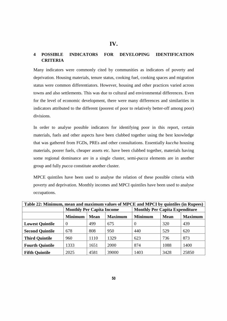
50
IV.
4 POSSIBLE INDICATORS FOR DEVELOPING IDENTIFICATION CRITERIA
Many indicators were commonly cited by communities as indicators of poverty and
deprivation. Housing materials, tenure status, cooking fuel, cooking spaces and migration
status were common differentiators. However, housing and other practices varied across
towns and also settlements. This was due to cultural and environmental differences. Even
for the level of economic development, there were many differences and similarities in
indicators attributed to the different (poorest of poor to relatively better-off among poor)
divisions.
In order to analyse possible indicators for identifying poor in this report, certain
materials, fuels and other aspects have been clubbed together using the best knowledge
that was gathered from FGDs, PREs and other consultations. Essentially kuccha housing
materials, poorer fuels, cheaper assets etc. have been clubbed together, materials having
some regional dominance are in a single cluster, semi-pucca elements are in another
group and fully pucca constitute another cluster.
MPCE quintiles have been used to analyse the relation of these possible criteria with
poverty and deprivation. Monthly incomes and MPCI quintiles have been used to analyse
occupations.
Table 22: Minimum, mean and maximum values of MPCE and MPCI by quintiles (in Rupees) Monthly Per Capita Income Monthly Per Capita Expenditure
Minimum Mean Maximum Minimum Mean Maximum
Lowest Quintile 0 499 675 0 320 439
Second Quintile 678 808 950 440 529 620
Third Quintile 960 1110 1329 623 736 873
Fourth Quintile 1333 1651 2000 874 1088 1400
Fifth Quintile 2025 4581 39000 1403 3428 25850

51
The indicators analysed are housing materials, main water source, main source of
lighting, cooking area, main cooking fuel, assets, social groups, education level, head of
households, households with disabled members, activity status of household members
and occupations.

52
4.1 Material of Roof
Thatch grass and tarpaulin roofs were the most common kuccha materials of roof that
were used in SMTs and were concentrated in the first three MPCE quintiles. However,
3.2 per cent of those in the fifth quintile and 7.4 per cent in the fourth quintile had such
roofs. In the case of asbestos and tin sheets, even though their use declined with
increasing MPCE quintiles, they constituted 36 per cent and 44.2 per cent of the fifth and
fourth quintiles respectively. Tiled and wooden roofs, which mainly belonged to older
houses were concentrated in the middle three quintiles and were lowest in the fifth
quintile. In the case of cement and brick roofed houses, there was a clear increase with
increase in quintiles, however almost one-fourth of both the first and second quintile were
households with cement and brick roofs. In case of roof indicators, the most kuccha roof
could be considered as an inclusion criteria, however, the more pucca roofs could not be
used as an exclusion criteria as a large number of the poorest of poor houses such roofs,
through the government support or even otherwise. (See Annexure 5 Table 17 for details)

53
4.2 Material of Floor
Flooring materials were more universal and were found across towns. In case of earthen
and semi-earthen flooring, there was a decreasing trend in quintiles, and only 8 per cent
of such households were present in the fifth quintile. However, 17 per cent of fifth
quintile households had earthen or semi-earthen flooring. Bricks and cement flooring
were more or less evenly spread across the first four quintiles, but were 16.4 per cent of
the fifth quintile. In case of households using chips, tiles or stone, there was a clear
increasing trend with increasing quintiles; however even in the lowest quintile more than
16 per cent of the households had chip, tile or stone flooring. Use of flooring material as
inclusion or exclusion criteria is likely to have errors. (See Annexure 5 Table 18 for
details)
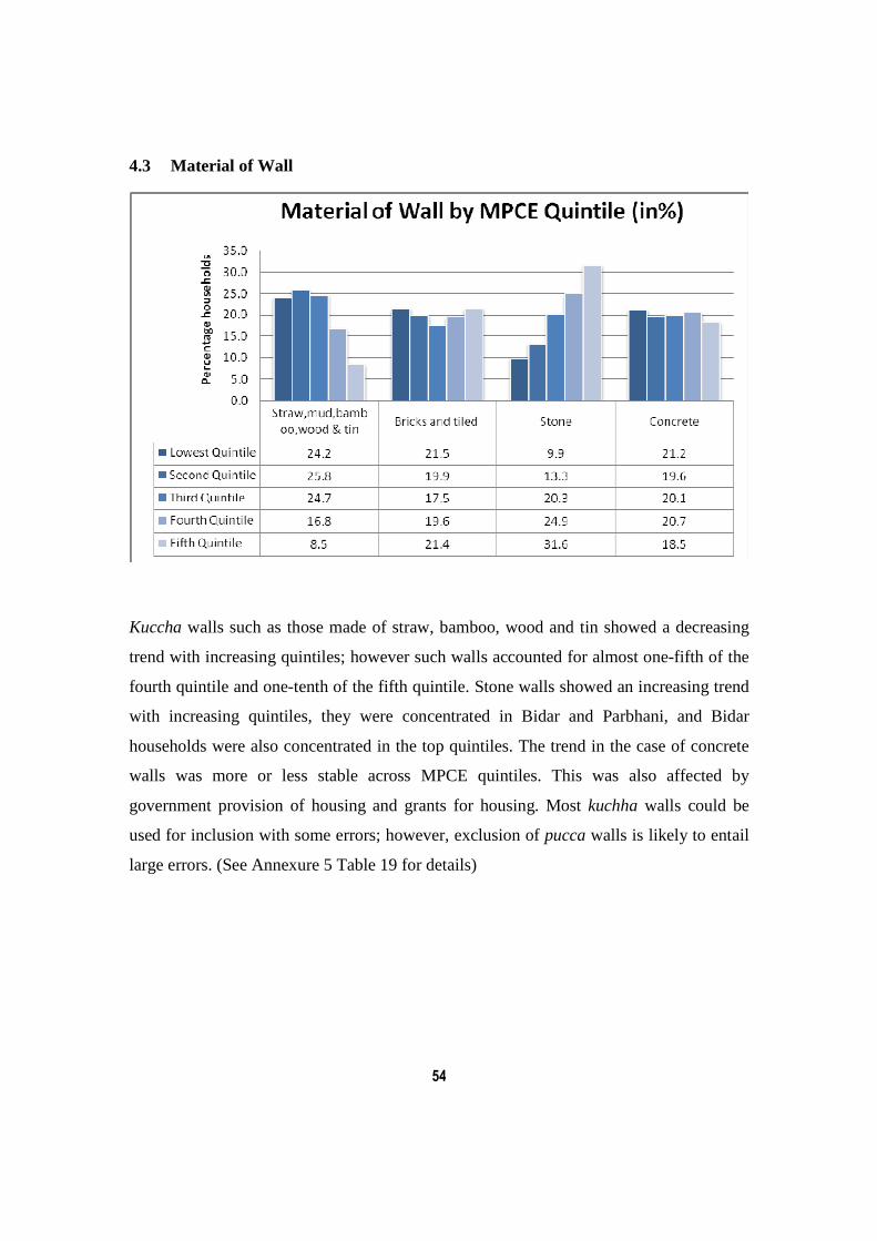
54
4.3 Material of Wall
Kuccha walls such as those made of straw, bamboo, wood and tin showed a decreasing
trend with increasing quintiles; however such walls accounted for almost one-fifth of the
fourth quintile and one-tenth of the fifth quintile. Stone walls showed an increasing trend
with increasing quintiles, they were concentrated in Bidar and Parbhani, and Bidar
households were also concentrated in the top quintiles. The trend in the case of concrete
walls was more or less stable across MPCE quintiles. This was also affected by
government provision of housing and grants for housing. Most kuchha walls could be
used for inclusion with some errors; however, exclusion of pucca walls is likely to entail
large errors. (See Annexure 5 Table 19 for details)

55
4.4 Main source of lighting
Households with electricity as the main source of lighting were more or less equally
distributed across MPCE quintiles. Households mainly depending on kerosene accounted
for only 9 per cent of the fifth quintile, but almost two-thirds of kerosene dependent
households were in the second and third quintiles. Kerosene use was dominant in
Madhubani (almost 70 per cent households were dependent on it) and Madhubani
households were also concentrated in the second and third quintiles. As mentioned
earlier, among the poor, the degree of deprivation could not be established by main
source of lighting or status of electrification as access to electrification was either
universal and where there was scarcity, entire settlements were not been covered, and
both the poorest of poor and the relatively well off amongst them had equal difficulty in
accessing them. However, kerosene dependent households were concentrated in the
bottom quintiles and only 9.6 per cent of households dependent on kerosene were in the
fifth quintile and compared to the population of the whole town, kerosene dependent
households were definitely poor. Therefore households lacking any electrification could
be included with little error, especially in towns with near universal electrification in poor
localities. (See Annexure 5 Table 20 for details)

56
4.5 Cooking area of households
• Those households with separate areas for cooking were indicated to be better-off
amongst the poor in all FGDs except in Jangaon and Bidar, where the nature of
housing had been strongly influenced by government benefits. Those households with
separate kitchens were concentrated in the top two quintiles, which constituted two-
thirds of such housing. However, the top two quintiles were mainly constituted by
Jangaon and Bidar households. Trends related to cooking areas were very region
specific and many preferred cooking outside or in courtyards. Other spaces such as
cooking in balconies, courtyards or settlement roads were more concentrated in the
lowest quintiles and only 14.3 per cent of such households were in the fifth quintile.
However, more than half of those in the fifth quintile were in the other space
category. Overall, those with separate kitchens could be excluded, but this would not
be without errors. Including those with no separate kitchens is likely to entail large
errors. (See Annexure 5 Table 21 for details)

57
4.6 Drinking water source
Only those households with private sources of water were indicated to be better-off
amongst poor. However, large sections, almost two-fifths of the lowest quintile
households were using a private source. Private sources were declining in higher
quintiles, showing little relation between private water source and expenditure of
households. Piped water supply was a little higher in the fifth quintile but households
were more or less equally divided in the quintiles. Those purchasing water were mostly in
Jangaon and were therefore concentrated in the last two quintiles. Public sources were
concentrated in the middle three quintiles but a little lesser in the fifth quintile. Overall
water supply was very town specific and no clear pattern could be observed to conclude
on the feasibility of inclusion or exclusion. (See Annexure 5 Table 23 for details)

58
4.7 Main Fuel used for Cooking
Poorer fuels such as firewood, leaves and wood shavings and other locally dominant fuels
such as coal, gobar gas, cow dung and agricultural waste showed decreasing use with
increasing quintiles. On the other hand, kerosene, electric sigri and LPG were increasing
with increasing quintiles. The first category of poor fuels and LPG were present in all
towns while the other two categories were more region specific. The first category of
poor fuels was concentrated in the first three quintiles but a considerable proportion was
also present in the fourth and fifth quintile. However, those using LPG were highly
concentrated in the top two quintiles and only 8.5 per cent were in the lowest quintile,
making the presence of LPG a better exclusion criterion than the use of poorer fuels as an
inclusion criteria. However, such exclusion criteria could not be used in areas where
government distribution and subsidies on stoves and LPG have been implemented. (See
Annexure 5 Table 24 for details)

59
4.8 Assets Categories 4
Category 1 households, which did not have any of the categorised assets were fewer in
the top two quintiles, though, 17.6 per cent and almost 15 per cent of fourth and fifth
quintile households fell in this category. In the case of category 2, even in the fourth
quintile, more than one-fifth of the households had cycles. The drop was very sharp in the
fifth quintile, where only 5.5 per cent households of those having cycles were present.
This was highly influenced by Jangaon households which were concentrated in the
highest two quintiles and only 0.4 per cent of its households fell in category 2. In
categories 3, 4 and 5; there was a increasing trend with increasing quintiles. However, a
4 Asset categories are as follows:
• Category 1: consists of households that do not possess any of the following assets - cycle, black and white television, exhaust fan,
colour television, water pump, refrigerator and air cooler.
• Category 2: consists of households which only possess a cycle out of all the assets mentioned in category 1.
• Category 3: consists of households which possess a black and white television or an exhaust fan, they may or may not possess a cycle,
but do not possess colour television, water pump, refrigerator and air cooler.
• Category 4: consists of households which possess a colour television or a water pump, they may or may not possess a cycle, black and
white television or an exhaust fan, but do not possess a refrigerator or air cooler.
• Category 5: consists of households which possess a refrigerator or air cooler and may or may not possess the other assets mentioned.

60
substantial percentage (16 per cent to 20 per cent) of the lowest quintiles constituted these
categories. (See Annexure 5 Table 22 for details)
Goods such as refrigerators and air coolers were being used by many poor households.
Even in the lowest monthly per capita expenditure (MPCE) quintile, about 10 per cent of
the households had a refrigerator or air cooler.
Assets such as four wheelers, heavy vehicles, air conditioners, computers, washing
machines, heaters and geysers were used by very few and relatively better-off
households. These could be used for exclusion, but they are also likely to entail very
small exclusion errors.
Household with bulbs/ tube light as the only electric gadgets could be identified as
poorest of poor.
4.9 Religion
Table 23: Religion by MPCI quintiles (in%)
Buddhist Chrisitan Hindu Muslim Sikh Total
Lowest Quintile 18.3 9.5 5.5 0.9 18.5 43.6 23.6 37.0 22.9 9.0 20.0 100
Second Quintile 21.9 11.2 6.8 1.1 19.6 46.0 21.0 32.5 23.5 9.2 20.2 100
Third Quintile 22.8 12.0 20.5 3.5 19.7 47.5 18.3 29.2 19.4 7.8 19.6 100
Fourth Quintile 25.9 13.1 24.7 4.1 20.6 47.6 18.2 27.8 19.4 7.4 20.4 100
Fifth Quintile 11.2 5.8 42.5 7.2 21.6 51.4 18.9 29.8 14.7 5.8 19.8 100
Total 100.0 10.3 100.0 3.4 100.0 47.2 100.0 31.2 100.0 7.8 100.0 100
Hindus were more or less equally distributed among both MPCE and MPCI quintiles but
demonstrated a slightly increasing trend with increasing quintiles. In the case of Muslims,
there was a decreasing trend with increasing MPCI quintiles but an increasing trend with
increasing MPCE quintiles. In the case of Sikhs and Buddhists, there was a decreasing
trend with increasing MPCE and MPCI quintiles. In the case of Christians, there was a

61
clear increasing trend with both increasing MPCE and MPCI. However, no clear
conclusion could be drawn regarding inclusion, exclusion or weighting. (See Annexure 5
Table 36. for details).
4.10 Caste Groups
Table 24: Caste Groups by MPCE quintiles (in%)
Scheduled
Caste Scheduled
Tribe
Other Backward
Caste General Muslim
caste Nomadic
Tribe Total Lowest Quintile 31.1 57.4 20.0 3.2 9.7 10.2 9.6 3.5 15.5 24.3 46.2 1.4 19.9 100.0 Second Quintile 23.6 43.2 20.0 3.2 16.3 17.0 13.5 4.8 19.9 31.0 23.1 0.7 20.1 100.0 Third Quintile 16.6 30.4 30.0 4.8 23.3 24.4 15.4 5.5 22.2 34.6 7.7 0.2 20.0 100.0 Fourth Quintile 17.6 32.3 20.0 3.2 21.5 22.6 25.6 9.2 20.5 32.0 23.1 0.7 20.0 100.0 Fifth Quintile 11.2 20.6 10.0 1.6 29.2 30.7 35.9 12.9 21.9 34.2 20.0 100.0 Total 100.0 36.8 100.0 3.2 100.0 21.0 100.0 7.2 100.0 31.2 100.0 0.6 100.0 100.0
Scheduled Castes demonstrated a clear declining trend with increasing MPCE quintiles.
Overall, Scheduled Tribes declined with increasing MPCE, however, this decline was not
consistent, and 30 per cent of the STs were concentrated in the third quintile. OBCs and
General castes demonstrated an increasing trend with increasing quintiles. This increase
was sharper and more clear in case of the general category. The number of nomadic tribe
households was too small for analysis. As such SCs and STs should be considered for
greater inclusionary weight.
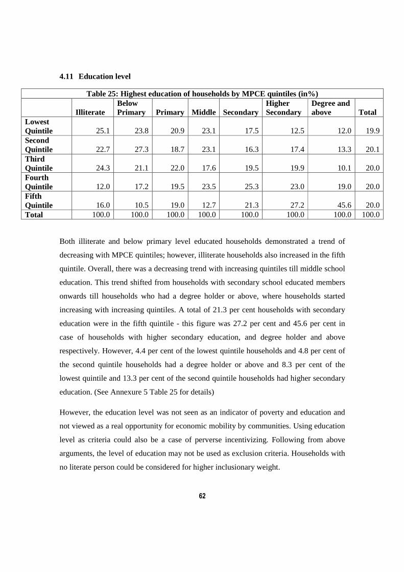
62
4.11 Education level
Table 25: Highest education of households by MPCE quintiles (in%)
Illiterate Below Primary Primary Middle Secondary
Higher Secondary
Degree and above Total
Lowest Quintile 25.1 23.8 20.9 23.1 17.5 12.5 12.0 19.9 Second Quintile 22.7 27.3 18.7 23.1 16.3 17.4 13.3 20.1 Third Quintile 24.3 21.1 22.0 17.6 19.5 19.9 10.1 20.0 Fourth Quintile 12.0 17.2 19.5 23.5 25.3 23.0 19.0 20.0 Fifth Quintile 16.0 10.5 19.0 12.7 21.3 27.2 45.6 20.0 Total 100.0 100.0 100.0 100.0 100.0 100.0 100.0 100.0
Both illiterate and below primary level educated households demonstrated a trend of
decreasing with MPCE quintiles; however, illiterate households also increased in the fifth
quintile. Overall, there was a decreasing trend with increasing quintiles till middle school
education. This trend shifted from households with secondary school educated members
onwards till households who had a degree holder or above, where households started
increasing with increasing quintiles. A total of 21.3 per cent households with secondary
education were in the fifth quintile - this figure was 27.2 per cent and 45.6 per cent in
case of households with higher secondary education, and degree holder and above
respectively. However, 4.4 per cent of the lowest quintile households and 4.8 per cent of
the second quintile households had a degree holder or above and 8.3 per cent of the
lowest quintile and 13.3 per cent of the second quintile households had higher secondary
education. (See Annexure 5 Table 25 for details)
However, the education level was not seen as an indicator of poverty and education and
not viewed as a real opportunity for economic mobility by communities. Using education
level as criteria could also be a case of perverse incentivizing. Following from above
arguments, the level of education may not be used as exclusion criteria. Households with
no literate person could be considered for higher inclusionary weight.
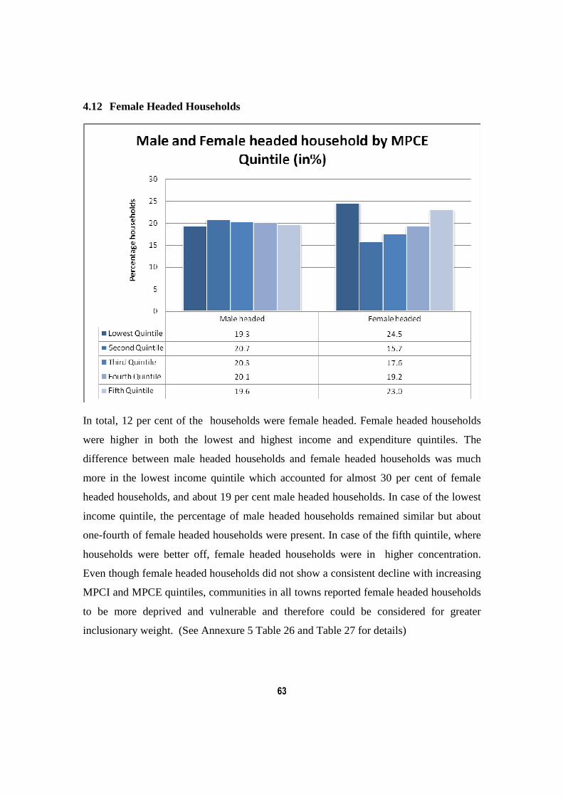
63
4.12 Female Headed Households
In total, 12 per cent of the households were female headed. Female headed households
were higher in both the lowest and highest income and expenditure quintiles. The
difference between male headed households and female headed households was much
more in the lowest income quintile which accounted for almost 30 per cent of female
headed households, and about 19 per cent male headed households. In case of the lowest
income quintile, the percentage of male headed households remained similar but about
one-fourth of female headed households were present. In case of the fifth quintile, where
households were better off, female headed households were in higher concentration.
Even though female headed households did not show a consistent decline with increasing
MPCI and MPCE quintiles, communities in all towns reported female headed households
to be more deprived and vulnerable and therefore could be considered for greater
inclusionary weight. (See Annexure 5 Table 26 and Table 27 for details)

64
4.13 Households with Disabled Persons
In total 8.3 per cent households had a disabled member and such households were highly
concentrated in the lowest two quintiles of both per capita income and expenditure. In
case of per capita expenditure almost 48 per cent of households with a disabled member
were in the lowest two quintiles while about 38 er cent of households without a disabled
member were in the lowest two quintiles. As in the case of female headed households, the
concentration of disabled households in the lower two MPCI quintiles was higher at 54.2
per cent Only 6.5 per cent of households in the fifth MPCE quintile had a disabled
member. Across both MPCE and MPCI, there was a clear trend of households with
disabled members being poorer. There is a clear case for giving greater inclusionary
weight to households having a disabled member. (See Annexure 5 Table 28 and Table 33
for details)

65
4.14 Activity Status
Table 26: Activity status of working and earning members in SMTs by MPCE quintiles (in %)
Lowest Quintile
Second Quintile
Third Quintile
Fourth Quintile
Fifth Quintile Total
Self Employed - Employer 0.1 2.0 1.2 2.7 7.9 2.5 Own account worker 25.3 23.4 25.0 24.4 27.8 25.0 Regular Wage / Salaried / Worker 15.3 18.3 23.2 24.0 29.3 21.6 Household based piece rate work 3.7 5.9 7.0 7.7 4.7 5.8 Casual wage labour 46.9 43.1 35.5 33.0 20.0 36.6 Unpaid family labour 1.3 2.4 2.2 2.9 1.9 2.2 Retired - Pensioner/ Widow Pensioner 3.2 2.8 3.4 4.9 7.6 4.2 Rentier 0.4 0.1 0.6 0.2 Beggar 3.9 2.1 2.5 0.4 0.2 1.9 Total 100.0 100.0 100.0 100.0 100.0 100.0
Self-employed employers were concentrated in the top two quintiles and there were only
1 per cent of self-employed persons in the lowest quintile. Own account workers were
more or less stable across quintiles due to a range of occupations falling in the category
across towns and workers ranging from hawkers, vendors, small shop owners, households
manufacturing, owners of small businesses and contractors. Regular wage and salaried
workers were slightly more concentrated in the higher quintiles but had a sizeable
proportion in the bottom quintiles as regular salaried persons also included domestic
workers and private sweepers. Household based piece rate work was concentrated in the
middle three quintiles. Its distribution within towns was concentrated in Jangaon and
Pakur and beedi making was mainly being carried out by women, who were not the main
household earners. Casual wage labourers were concentrated in the bottom quintiles,
though 8.8 per cent of casual wagers were in the fifth quintile while 20 per cent of
households in the fifth quintile were casual wagers. Almost 45 per cent of beggars were
in the bottom quintile, followed by 50 per cent in the second and third quintiles. Only
about 5 per cent were in the top two quintiles. In the bottom most quintile, almost 4 per

66
cent households were beggars but only 0.6 per cent were beggars in the top two quintiles.
(See Annexure 5 Table 29 for details)
Unpaid family labour was also concentrated in the middle quintiles such as in the case of
household based piece rate work. Pensioners were concentrated more in the top two
quintiles, though no conclusion can be drawn as no differentiation has been made
between widow pensioners, government retired pensioners, disabled pensioners and other
pensioners. No clear conclusion can be drawn for households living on rent due to small
sample.
Overall, self-employed employers were clearly more concentrated in the top two
quintiles, beggars in the bottom two and there was a clear trend in the case of casual
wagers being poorer. For other activity status, no clear conclusion could be drawn.
4.15 Occupation of household
Occupations of workers such as construction labour, agricultural labour, cobblers,
headload workers, rickshaw pullers, cart pullers, hotel waiters, rag pickers, scrap
workers, private sweepers, domestic workers, and helpers showed a clear decline with
increasing MPCI quintiles.
Workers such as welders, carpenters, polishers, fabricators, electricians, higher
professionals such as doctors and engineers, small business owners, contractors, raj
mistri, masons and government employees showed an increase with increasing MPCI
quintiles. (See Annexure 5 Table 35 for details)
Households with government teachers and doctors had the highest MPCI of Rs.9,425 and
highest MPCE of Rs. 3,493. They were followed by households with engineers and
doctors, those in security forces, other middle level government employment. Private
teachers, small business owners, construction and other supervisors, government peons
and drivers, privately employed lower level administrative staff, and government
sweepers, had MPCI of more than Rs.2,500 and MPCE of more than Rs. 1,700. (See
Annexure 5 Table 34 for details)
67
Households with welders, carpenters, plumbers, electricians, saw mill labour, traditional
artisan, hawkers and vendors, tailors, auto drivers, other drivers, mistris, masons, shop
owners, small household manufacturers, tea, pan and beedi shop owners, salesman, repair
mechanics, nurse, ward boys, shop assistants, priests, barbers had a MPCI between Rs.
1,500 and Rs.2,500 and MPCE between Rs.1,000 and Rs.2,000.
Cobblers had the lowest MPCI of Rs. 852, followed by beggars at Rs. 1,004 and rag
pickers at Rs. 1,096. Households with cobblers, beggars, rag pickers, unskilled casual
wage labourers and rickshaw pullers could be automatically included with little error.
Table 24: Ranking of Poor Occupations
Poorest of Poor Better Off Amongst Poor Relatively well-off
• Rag pickers, Beedi makers
• Rickshaw and Thela pullers
• Live by begging
• Main earner working as agricultural labour
• Those migrating for work from Madhubani and Pakur
• Attached agricultural migrants from Parbhani and Mansa
• Unskilled casual wage labourers
• Raj Mistri and Mason
• Painter
• Carpenter
• Tailors
• Small shops and business
• Work in hotels etc
• Teachers
• Municipality job
• Other government job
• Contractors
• Small enterprise owners

68
V.
5 PUBLIC DISTRIBUTION AND PRESENT TARGETING FOR WELFA RE BENEFITS IN SMTs
Table 27: Public distribution cards possessed by households in SMTs (in%)
Parbhani Bidar Mansa Madhubani Jangaon Pakur Total APL (Above Poverty Line) 11.0 15.8 40.1 16.7 5.0 7.1 16.2 BPL (Below Poverty Line) 46.4 70.8 14.6 48.1 75.5 41.4 50.9
Antoydaya 3.5 3.1 22.1 7.1 11.4 6.7
Blue card and other 35.7 0.3 0.5 5.3 Do not have any card 39.1 10.3 9.6 12.8 12.4 39.5 20.9
Total 100.0 100.0 100.0 100.0 100.0 100.0 100.0
Table 28: Public Distribution Cards possessed by households by MPCE quintiles (in%)
APL
BPL ,Antoydaya and
Other
Do not have any
Card Total Lowest Quintile 15.4 21.3 19.5 19.9 Second Quintile 18.2 19.2 24.1 20.1 Third Quintile 20.8 19.4 21.5 20.0 Fourth Quintile 23.1 19.0 20.8 20.0 Fifth Quintile 22.5 21.2 14.2 19.9 Total 100 100 100 100
Public distribution of food items and kerosene to households was present in all SMTs. In
total, about 21 per cent of the sample households reported not having APL, BPL,
Antoydaya or other cards. This percentage was very high in Parbhani and Pakur,
constituting almost 40 per cent of the households and was the lowest in Mansa where
almost one-tenth households did not have any card. In terms of regularity and amount due
for dispersals, Madhubani and Pakur households reported issues on both fronts. Both
issues were reported in Parbhani, Bidar and Mansa, but were lesser in degree than

69
Madhubani and Pakur. In Mansa, the Punjab government had given out cards known as
'blue' cards to households. In case of Jangaon, households reported regular disbursements
and apart from rice, wheat, sugar and kerosene, BPL card holders also received
detergents, soaps, oil, pulses and salt.
Approximately half of the households reported having BPL cards, one-fourth of the
households reported not having any card, followed by those with Antoydaya cards and
other cards such as the blue card in Punjab.
Overall, seen in relation with MPCE quintiles, there was an increase in APL cards with
increase in quintiles. Also12.5 per cent, 14.7 per cent and 16.8 per cent of first, second
and third quintiles respectively had APL cards. A greater percentage of 20.4 per cent, 25
per cent and 22.4 per cent of first, second and third quintiles had no cards. Of all
quintiles, the fifth quintile had the lowest percentage of households which did not have a
card. Households with a BPL/Antoydaya or other card were more or less uniform across
the quintiles, but were slightly higher in the first and fifth quintile. The trends were
similar in case of MPCI quintiles (See Annexure 5 Table 37 and Table 38 for details)
This shows that targeting for present welfare benefits has many inclusion and exclusion
errors, as 20 per cent of the lowest quintile did not have any card and 25 per cent of the
second quintile did not have any card. Similarly 12.5 per cent of the lowest quintile
households had APL cards, and 14 per cent of second quintile households had APL cards.

70
VI.
6 CONCLUDING SUMMARY
• Present targeting of poor for public distribution of food in SMTs was poor. Of the
indicators assessed for their relation with per capita expenditure, no indicator was
universal or extremely sensitive for identifying poor.
• Household criteria based on public goods and town connectivity such as electricity in
the household, water supply and piped water showed little difference across
expenditure quintiles. These services were definitely better available to the richer
sections, but within the poorer groups, they were equally difficult to access for even
the relatively – well off.
• In places with high disbursement of government benefits hidden poverty was not
captured by criteria such as housing, fuels and assets etc. Dependency on such
benefits was also very high. The danger of excluding poor and vulnerable households
is very high, particularly in some states and regions making it imperative to account
for government benefits in these areas and states.
• Some issues with present Sate-specific criteria and targeting were raised by
municipality staff and residents; such as where the possession of a cell phone was
reported as being used as exclusion criteria. Similarly, where brick housing was being
excluded from benefits, households complained that even though their walls were
made of bricks, they had only been stacked and had no mortar, making their housing
vulnerable. This merits careful surveying and incorporating nuances of building
materials and layout in order to capture housing and other vulnerabilities.
• With little inclusion error, poor settlements in towns such as Madhubani and Pakur as
a whole can be identified as poor, due to homogenous nature of settlements; this
would not be possible in other towns. In Jangaon, for instance there are settlements
where middle income households, rich households and very poor are living together,

71
mainly due to soaring demand for land and gentrification due to availability of basic
services in these settlements.
• When compared with bigger cities and towns, it is not surprising that issues related to
precariousness of housing conditions and tenure are muted in SMTs. However, the
two bigger SMTs show a greater degree of precariousness and an increasing tendency
towards precariousness.
• Dominance of regional materials, regional fuels and regional practices is high in
SMTs – for example, the use of stone and khapra and local fuels. Regional elements
may not be as dominant in bigger cities and towns.
• It was also noted that the value of materials changed with passage of time and
availability of newer materials – for example, kaveli/ khapra were the only option
after thatched roofs in Pakur. These tiles are now considered more expensive due to
the availability of other cheaper materials such as bricks, tin and asbestos.
• In case of the six SMTs, there was also an issue in valuation of indicators due to
regional and local supplies and subsidies– for example, coal may not be considered a
cheap fuel, but is very cheaply available in Pakur (Jharkhand) and is being used by a
large majority of poor. This makes it important to understand the relative values of
housing materials and other indicators in a regional context before using them for
purposes of inclusion, exclusion or greater weight.
• Issues related with hidden poverty due to disbursement of benefits, use of regional
fuels and construction material, different valuations of materials across time and
regions indicate the need for a regional approach to identification of the poor. It
becomes imperative that some regional criteria should be included in the
identification process with a view to address issues of relative and absolute poverty
across towns and states.
72
VII.
7. ANNEXURES
Annexure 1: Questionnaire (attached separate file)

73
Annexure 2: FGD and PRE guidelines
1. Background information
• When was the community founded?
• What are the geographical limits of the community?
• What public services are there in the community, and how much of the population
is covered (approximately)? (E.g. piped water – two-thirds, electricity – one
thirds, etc.)
• How many households are there in the community? How many people per
household? What proportion of the population is male, and what proportion is
female?
• Do people own their land or do they rent? What is the average rent?
• What are the major caste groups and their approximate proportions?
• Are there any recent migrants in the population? Where have they come from?
• Do many people own a vehicle? What sort? (four wheel, two wheel, bicycle, etc.)
• What are the major sources of income of the population, for men and for women?
How many households have a regular income?
2. Problems
• Ranked listing of the main problems of the FGD Group ranging from
infrastructural constraints, lack of public services like water, sanitation,
electricity, toilets, lack of economic opportunities, conditions of work,
environmental problems such as flooding and water logging etc, access to health
services, access to credit, quality of healthcare, quality of teaching and others.
3. Social groups
• Which are the main social groups that live in this settlement?
• What work are these groups involved in?
• Are there any occupational groups?
74
• Other than caste groups, are there any other social or occupational groups?
• Are there any female headed households, houses with single women, houses with
the women, sick and disabled
• Are there any migrants in the group or in the community? If so, who are they,
where have they come from, have they migrated permanently or do they do so
seasonally and why do they migrate? What occupations are they involved in?
4. Occupation
• What are the main occupations people are involved in and what their background
is? what difficulties do they face?
5. Ration
• How many households have ration cards? Where did they get it from? • Where does one get their ration from, when was the last time one went to get
ration and from where? How far is the ration shop from their settlement?
6. Housing
• What kind of housing does the settlement have? Is it kuchha, pukka, semi kuchha or semi- pucca?
• What are the problems that one faces with this kind of housing? Problems ranging from water logging, flooding, degradation?
7. Education
• How many schools are there in the community (Primary, Secondary, Colleges)
and how far are they?
• How many children from the settlement go to schools and which schools? How
many girl and how many boys go to these schools?
• Is the quality of education good or bad?
• Do the schools have facilities for the children such as toilets, water, food,
classrooms etc.

75
8. Health
• Any hospitals nearby? Are they government or private hospitals and what is the
level of facilities in each? Are the services easily accessible?
• What are the problems when one approaches the hospital to gain services?
• What kind of diseases are the there in this community? Do people suffer
frequently and what are the reasons for this?
• How much of one’s ,monthly income is spent on health expenses?
9. Ranking exercise
The FGD groups are asked to identify who they think are the poor and what their characteristics are:
• Who are the poorest?
• Can one categorise the poor into two to five specific categories depending on their
degree of deprivation, poverty and vulnerability?
• Characteristics of each category in terms of housing, social and economic
background, and occupations of these categories. Other criteria such as:
� Households with elderly members, or disabled members, or female headed
households, or members with health problems.
� Those who are part of weaker economically or socially weaker groups.
� Those working in particular occupations such as sweeping, cleaning or in
casual work
� Those living in particular kind of housing
� Those households that lack access to basic services such as toilets,
drainage, kitchens or based on assets they don’t have
� Those households that migrate
� Households that don’t have regular income, or very little income
76
10. Reasons for poverty
• Caste
• Illness
• Particular kind of occupation
• Loss of an earning member
• Discrimination
• Loans/debt
• Theft/damage
• Lack of Education
• Lack of political participation
• Lack of Insurance
11. Ways to move out of poverty
• Better Education
• Better Skills
• Easy availability of Loans
• Access to Public Services
• Best access to economic opportunities
• Better policies

77
Annexure 3: Methodology for obtaining Income Data
Income data has been collected to understand it’s relation with occupations and
household characteristics such as educational attainment, basic amenities, access to basic
services and present status of government targeting for disbursement of welfare benefits.
Individual Incomes: Income data has been obtained for each earning member including
renters and pensioners. Individual income has been collected on a monthly basis.
Information regarding each individual’s primary activity and secondary activity, their
detailed occupation, industry and location of work place was first collected.
Subsequently, households were asked to calculate each individual member’s monthly
income averaged over last 12 months. For example, if a construction labour earns Rs. 150
per day for 20 days a month for 9 months and earns Rs. 150 per day for 10 days a month
for 3 months. His total income for the year which was Rs.31500 was divided by 12
months to obtain monthly income of Rs.3375. Both primary and secondary incomes were
collected in the same manner.
Household Incomes: Incomes which were earned by the household such as rent from
land or other assets, remittances and other sources were accounted for in a separate
section and were collected on a monthly and yearly basis, depending on the intervals at
which the household was receiving them.
The total monthly household income has been computed by adding the total monthly
primary income of each household, total monthly secondary income of each household
and total of monthly other incomes of each household.
Annexure 4: Methodology for obtaining Expenditure Data
Expenditure details of each household have been collected for the last one month.
Expenditure data for predefined food and non-food heads has been collected and
expenditure under other miscellaneous heads as reported by the households has also been
collected.
Expenditure on food was divided into cereal and pulses, fruits, vegetables, milk and milk
products, fish, meats and poultry, condiments such as oil, spices, sugar etc, Intoxicants

78
such as alcohol, cigarettes etc. While collecting data on food heads, households were first
asked to calculate amount of food obtained through PDS systems and to first calculate
related expenditure for each head. Households were then asked to calculate remaining
food items bought on a monthly basis, weekly basis and daily basis and the amount spend
on each of these items was calculated accordingly.
Health expenditure, education related expenditure, loan repayment, expenditure on
household goods, expenditure on rentals, expenditure on transport were the predefined
non-food heads. Expenditure of the household under these heads in the last one month
was calculated.
Households were also asked to share other expenditures in the last month which could not
be accounted for under the predefined heads. Mobile bills, electricity bills, water bills and
expenditure on buying water, satellite television bills, soaps, detergents etc were common
other expenditures reported by the households.
The total household expenditure has been computed by adding food expenditure, non-
food expenditure and other expenditure incurred by the household in the last month.

79
Annexure 5: Tables
Annex Table 1: Sample Profile and Demographic Profile in SMTS
No. of households
Percentage households
Sample Population
Avg. household size
Dependency ratio
Parbhani 545 25 2795 5.1 0.62 Bidar 545 25 2291 4.2 0.62 Mansa 314 14 1567 5.0 0.66 Madhubani 312 14 1805 5.8 0.91 Jangaon 242 11 747 3.1 0.46 Pakur 210 10 908 4.3 0.82 Total 2168 100 10113 4.7 0.67
Annex Table 2: Religion and Caste composition in SMTs (in%) Parbhani Bidar Mansa Madhubani Jangaon Pakur Total Hindu - SC 9.9 22.0 33.1 9.6 23.1 20.0 18.7 Hindu - ST 0.7 9.9 0.6 0.8 3.3 3.2 Hindu - OBC 3.1 7.3 1.9 46.8 51.7 39.0 19.2 Hindu - General 3.3 9.9 9.9 5.1 2.1 4.3 6.1 Hindu - Total 17.1 49.2 44.9 62.2 77.7 66.7 47.2 Muslim - other than OBC 40.9 12.1 3.5 6.7 14.9 10.5 17.5 Muslim - OBC 0.7 26.1 31.1 4.1 21.4 13.7 Muslim - Total 41.7 38.2 3.5 37.8 19.0 31.9 31.2 Buddhist-Total 39.4 1.3 0.6 10.3 Sikh-Total 1.7 0.2 50.6 0.5 7.8 Christian-Total 0.2 11.2 0.3 3.3 1.0 3.4 Religion -Total 100.0 100.0 100.0 100.0 100.0 100.0 100.0
Annex .Table 3: Distance of household from main source of drinking water in SMTs (in%) Parbhani Bidar Mansa Madhubani Jangaon Pakur Total Inside residence 21.5 28.3 72.6 28.5 11.6 6.7 29.1 Right outside residence 25.1 36.7 18.8 16.0 5.4 10.5 22.2 Within 50 meters radius 45.0 28.8 6.7 43.9 17.8 44.3 32.1 Within 500 metres radius 8.3 3.5 1.6 10.9 57.0 38.1 14.8

80
Within 1 kilometer radius 0.2 2.4 6.6 0.5 1.4
Between 1 kilometer and 5 kilometers 0.2 0.3 1.2 0.2
More than 5 kilometers radius 0.2 0.6 0.4 0.2 Total 100.0 100.0 100.0 100.0 100.0 100.0 100.0
Annex. Table 4: Electrification status in SMT households (in%) Parbhani Bidar Mansa Madhubani Jangaon Pakur Total Metred electricity 95.6 72.3 80.6 25.6 97.9 60.5 74.4
Privately arranged from electricity poles 2.8 16.9 17.5 2.6 6.2 8.4 Do not have electricity 1.7 10.8 1.9 71.8 2.1 33.3 17.2 Total 100.0 100.0 100.0 100.0 100.0 100.0 100.0
Annex. Table 5: Occupation of households with no working age members (15 years to 59 years) in SMTs (in%)

81
Construction labour 2.5 Agricultural labour 6.2 Boot Polish & Cobbler 3.7 Agri and construction workers (any) 1.2 Other specalised casual labour (saw mill/ ara machine etc) 1.2 Welders/carpenters/polishers/fabricator/electricians 1.2 Animal husbandry and fishing 2.5 Traditional Artisans (goldsmith/kitemaker/weaver/bidri work) 1.2
Vegetables, fruits, fish and poultry hawkers and vendors 3.7 Other food & NF vendors 2.5 Beedi making and garland making 4.9 Rag picker & scrap worker 2.5 Tailoring 2.5 Sweepers (Pvt. ) 2.5 Beggar 8.6 Specialised Mistri, Mason 1.2 Domestic workers/utensil washing /laundry 8.6 Shop owners 6.2 Small hhld manufacturing (food&NF) 4.9 Lower level administrative work (Pvt.) 1.2 Small shop owners (Pan/Tea/Toddy/Beedi) 1.2 Watchman/ Security guard/ Gardner 2.5 Employee/ Job 1.2 Government peon & drivers 1.2 Pensioner 23.5 Rentier 1.2 Total 100.0
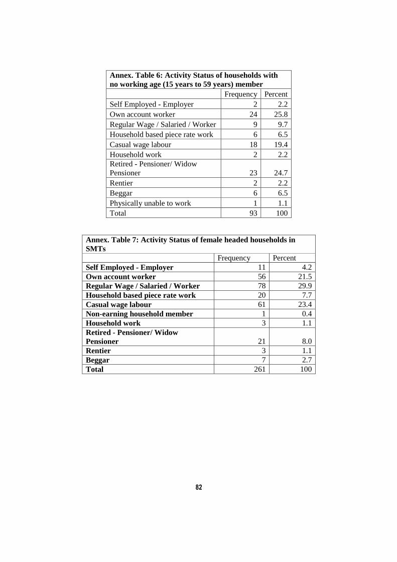
82
Annex. Table 6: Activity Status of households with no working age (15 years to 59 years) member Frequency Percent Self Employed - Employer 2 2.2 Own account worker 24 25.8 Regular Wage / Salaried / Worker 9 9.7 Household based piece rate work 6 6.5 Casual wage labour 18 19.4 Household work 2 2.2 Retired - Pensioner/ Widow Pensioner 23 24.7 Rentier 2 2.2 Beggar 6 6.5 Physically unable to work 1 1.1 Total 93 100
Annex. Table 7: Activity Status of female headed households in SMTs Frequency Percent Self Employed - Employer 11 4.2 Own account worker 56 21.5 Regular Wage / Salaried / Worker 78 29.9 Household based piece rate work 20 7.7 Casual wage labour 61 23.4 Non-earning household member 1 0.4 Household work 3 1.1 Retired - Pensioner/ Widow Pensioner 21 8.0 Rentier 3 1.1 Beggar 7 2.7 Total 261 100

83
Annex. Table 8: Occupations of female headed households in SMTs (in%) Construction labour 8.7 Agricultural labour 6.6 Headload workers 0.4 Factory labour 0.4 Other specalised casua labour (saw mill/ ara machine etc) 2.9 Rickshaw Pulling & cart pulling 0.8 Welders/carpenters/polishers/fabricator/electricians 0.8 Waiter/ Hotel labour/ catering labour/Cook 2.5 Animal husbandry and fishing 0.4 Traditional Artisans (goldsmith/kitemaker/weaver/bidri work) 0.4 Painter 0.4 Teacher & Librarian (Pvt.) 1.2 Higher professional and technical services (Engineer&Doctor) 0.4 Vegetables, fruits, fish and poultry hawkers and vendors 2.9 Other food & NF vendors 3.3 Small businesses owners/contractor/ supplier/supervisor 0.8 Beedi making and garland making 6.6 Rag picker & scrap worker 3.3 Auto Driver 0.4 Tailoring 3.7 Sweepers (Pvt. ) 3.3 Beggar 3.7 Specialised Mistri, Mason 1.2 Domestic workers/utensil washing /laundry 12.0 Drivers 1.2 Shop owners 6.6 Small hhld manufacturing (food&NF) 2.9 Lower level administrative work (Pvt.) 0.8 Small shop owners (Pan/Tea/Toddy/Beedi) 0.8 Salesman/broker/chit fund/real estate 0.8 Repair mechanic - (motor/ cycle/ watch) 0.4 Specialised assistants & other helpers 0.4 Watchman/ Security guard/ Gardner 0.8 Nurse/ Ward boy /ANM nurse 1.7 Shop assistants 2.1 Political repres./Jajmani act./Social workers 0.8 Employee/ Job 0.8 Security forces & other gvt.middle level staff 2.5 Government peon & drivers 1.2 Municipality and gvt. sweepers 0.4 Pensioner 7.0 Rentier 1.2 Total 100.0

84
Annex. Table 9: Activity Status of Girls and Boys in the age group 6 to 14 years in SMTs (in%) Parbhani Bidar Mansa Madhubani Jangaon Pakur Total Own account worker Male 6.6 1.8 1.0 Own account worker Female 0.4 2.9 0.5 Regular Wage / Salaried / Worker Male 0.4 0.8 0.8 0.5 Regular Wage / Salaried / Worker Female 0.9 0.7 1.7 0.5 Casual wage labour Male 2.7 0.8 1.5 2.3 1.6 Casual wage labour Female 1.4 0.4 Household based piece rate work Female 0.8 0.1 Non-earning household member Male 0.4 0.4 2.2 1.6 2.8 1.1 Non-earning household member Female 4.4 0.5 2.5 0.9 Student Male 90.1 83.3 62.8 82.0 98.1 79.8 82.4 Student Female 86.3 82.7 59.6 83.1 96.9 79.7 81.3 Household work Male 0.4 0.8 1.6 0.7
Household work Female 7.5 2.7 16.2 5.9 7.6 6.8 Physically unable to work Male 0.4 1.3 0.7 0.4 0.9 0.7 Physically unable to work Female 0.3 0.5 0.8 0.3 Beggar Male 3.3 0.7 0.9 Beggar Female 0.9 0.2 Not engaged in any activity Male 5.7 9.2 25.5 11.3 1.9 14.7 11.2 Not engaged in any activity Female 4.4 12.4 16.2 10.0 3.1 6.8 9.0 Total Male 100.0 100.0 100.0 100.0 100.0 100.0 100.0 Total Female 100.0 100.0 100.0 100.0 100.0 100.0 100.0

85
Annex. Table 10:Education level of Males and Females in the age group 10 to 20 years (in%) Parbhani Bidar Mansa Madhubani Jangaon Pakur Total Illiterate Male 4.77 8.57 30.14 13.86 10.92 11.33 Illiterate Female 4.43 8.99 26.56 8.70 8.13 9.61 Below Primary Male 4.30 6.35 11.00 23.22 1.20 10.92 9.70
Below Primary Female 4.43 6.83 13.02 22.71 22.76 10.80 Primary Male 17.66 13.02 11.00 17.98 8.43 26.89 15.93 Primary Female 17.45 17.99 11.46 22.22 13.33 18.70 17.32 Middle Male 28.16 16.51 9.57 14.61 6.02 24.37 18.63 Middle Female 25.52 13.67 13.54 13.04 13.33 25.20 18.27 Secondary Male 23.15 29.52 19.14 14.98 36.14 15.97 22.59
Secondary Female 29.43 30.58 17.19 12.56 24.00 14.63 23.27 Higher Secondary Male 17.42 21.90 12.92 7.12 25.30 6.72 15.37
Higher Secondary Female 14.06 16.19 11.98 8.70 28.00 8.13 13.58 Degree and above Male 4.53 4.13 6.22 8.24 22.89 4.20 6.44 Degree and above Female 4.69 5.76 6.25 12.08 21.33 2.44 7.15 Total Male 100.00 100.00 100.00 100.00 100.00 100.00 100.00
Total Female 100.00 100.00 100.00 100.00 100.00 100.00 100.00
Annex. Table 11 :Education level of Males and Females in the age group 30 to 40 years (in%) Parbhani Bidar Mansa Madhubani Jangaon Pakur Total Illiterate Female 4.7 9.1 20.8 17.7 11.8 10.5 Illiterate Male 4.4 11.5 22.4 13.3 1.3 9.5 10.5 Below Primary Female 7.9 8.6 16.0 25.9 4.4 19.1 12.9 Below Primary Male 7.7 7.9 19.4 24.1 9.3 29.8 14.4 Primary Female 18.9 15.2 13.6 15.6 16.2 32.4 17.6 Primary Male 20.6 17.6 15.7 15.8 14.7 23.8 18.1 Middle Female 27.6 13.6 12.8 8.8 10.3 10.3 16.3 Middle Male 27.8 15.0 11.2 10.8 13.3 13.1 16.8 Secondary Female 21.7 28.8 20.8 16.3 32.4 11.8 22.3 Secondary Male 20.2 27.3 16.4 13.9 33.3 10.7 20.5 Higher Secondary Female 13.8 19.7 11.2 4.8 22.1 10.3 13.6

86
Higher Secondary Male 13.3 15.0 12.7 9.5 14.7 4.8 12.3 Degree and above Female 5.5 5.1 4.8 10.9 14.7 4.4 6.9 Degree and above Male 6.0 5.7 2.2 12.7 13.3 8.3 7.3 Total Female 100.0 100.0 100.0 100.0 100.0 100.0 100.0 Total Male 100.0 100.0 100.0 100.0 100.0 100.0 100.0
Annex. Table 12: Occupations of working and earning members in SMTs (in%) Female Male Total Construction labour 8.2 18.0 15.7 Agricultural labour 13.4 2.6 5.1 Boot Polish & Cobbler 0.3 3.0 2.4 Brick Kiln worker 0.9 0.9 0.9 Headload workers 1.3 2.7 2.4 Agri and construction workers (any) 0.6 1.5 1.2 Factory labour 0.5 1.2 1.1 Other specalised casua labour (saw mill/ ara machine etc) 3.5 2.9 3.0 Rickshaw Pulling & cart pulling 0.3 3.8 3.0 Welders/carpenters/polishers/fabricator/electricians 0.5 1.9 1.6 Waiter/ Hotel labour/ catering labour/Cook 1.7 3.5 3.1 Animal husbandry and fishing 0.7 0.8 0.8 Traditional Artisans (goldsmith/kitemaker/weaver/bidri work) 0.2 1.4 1.1 Painter 0.1 2.4 1.9 Teacher & Librarian (Pvt.) 1.7 0.8 1.0 Higher professional and technical services (Engineer&Doctor) 0.1 0.5 0.4 Vegetables, fruits, fish and poultry hawkers and vendors 2.5 2.5 2.5 Other food & NF vendors 2.7 1.7 1.9 Small businesses owners/contractor/ supplier/supervisor 0.2 1.0 0.8 Beedi making and garland making 14.7 1.1 4.3 Rag picker & scrap worker 6.7 3.5 4.3 Auto Driver 0.1 2.9 2.2 Tailoring 4.5 2.6 3.0 Sweepers (Pvt. ) 1.7 0.2 0.6 Beggar 4.3 1.5 2.1 Specialised Mistri, Mason 0.8 4.7 3.8 Domestic workers/utensil washing /laundry 13.7 0.6 3.7 Drivers 0.2 3.7 2.9 Shop owners 3.9 6.1 5.6 Small hhld manufacturing (food&NF) 2.0 1.4 1.5 Lower level administrative work (Pvt.) 0.2 0.8 0.7 Small shop owners (Pan/Tea/Toddy/Beedi) 0.5 1.9 1.6

87
Salesman/broker/chit fund/real estate 0.5 1.4 1.2 Computer operator/videographer/photographer 0.5 0.4 Repair mechanic - (motor/ cycle/ watch) 0.8 2.3 2.0 Specialised assistants & other helpers 0.6 1.7 1.5 Watchman/ Security guard/ Gardner 0.3 1.0 0.8 Nurse/ Ward boy +ANM nurse 0.7 0.2 0.4 Shop assistants 1.4 4.3 3.6 Jajmani activities Priest and Barber 0.7 0.6 0.7 Employee/ Job 0.2 0.4 0.4 Government Teacher/ Doctor 0.5 0.6 0.6 Security forces & other gvt.middle level staff 0.3 0.8 0.7 Government peon & drivers 0.8 1.6 1.4 Municipality and gvt. sweepers 0.2 0.3 0.3 Total 100.0 100.0 100.0
Annex. Table 13: Activity Status of males and females in the age group 15 to 59 years (excluding students) in SMTs (in%) Parbhani Bidar Mansa Madhubani Jangaon Pakur Total Self Employed - Employer
Male 0.7 5.3 0.5 3.7 8.8 0.9 3.0 Female 0.6 1.8 1.7 3.4 1.2
Own account worker
Male 17.5 25.9 36.1 31.5 26.8 29.6 26.6 Female 9.1 16.0 45.7 35.0 16.0 9.0 18.7
Regular Wage / Salaried / Worker
Male 15.7 25.6 20.3 26.0 31.1 28.2 22.9 Female 26.7 18.7 22.9 26.7 14.3 24.6 21.8
Household based piece rate work
Male 1.0 3.0 0.5 4.6 7.9 2.8 2.7 Female 4.0 5.8 1.9 5.0 39.5 54.9 17.2
Casual wage labour
Male 61.0 32.3 38.5 24.7 23.2 31.5 38.9 Female 54.0 36.0 26.7 18.3 24.4 4.1 30.9
Non-earning household member
Male 0.1 0.6 0.7 6.2 1.9 1.5 Female 1.1 5.3 8.3 2.5 2.7
Retired - Pensioner/ Widow Pensioner
Male 1.0 1.3 0.2 0.5 0.9 0.5 0.8
Female 2.8 4.9 1.9 2.5 2.5 3.0
Rentier Male 0.2 0.0 Female 0.6 0.1
Beggar Male 0.1 3.4 0.9 Female 1.1 9.8 1.7 0.8 3.2
Unemployed Male 2.8 2.3 3.1 3.0 1.3 4.6 2.8 Female 1.8 1.0 3.3 1.6 1.1

88
Total Male 100.0 100.0 100.0 100.0 100.0 100.0 100.0 Female 100.0 100.0 100.0 100.0 100.0 100.0 100.0
Annex. Table 14: Mean Income of occupations and mean monthly per capita income and expenditure of households with those occupations in SMTs (in Rupees)
Parbhani
Bidar
Mansa
Madhubani
Jangaon
Pakur
Total
MPCI
MPCE
Mean Mean Mean Mean Mean Mean
Mean Mean Mean
Construction labour 2986 3746 2646 2725 5800 2278 3036 1328 730
Agricultural labour 1995 2015 2404 1042 1729 . 2005 1350 631
Boot Polish & Cobbler 3167 2900 1848 3500 . 1640 2100 852 500
Brick Kiln worker 2429 4250 4182 . 2200 . 3197 1905 641
Headload workers 2912 3412 3105 3500 2700 2333 3132 1307 731 Agriculture and construction workers (any) 3000 2500 2664 2400 3500 2200 2652 1295 926
Factory labour 2367 3000 3900 3213 3200 3000 3162 1606 956 Other specalised casual labour (saw mill/ ara machine etc) 2493 3818 6600 2125 3632 2596 3309 1721 1076 Rickshaw Pulling & cart pulling 2491 3150 4167 3563 3767 2780 3155 1152 741 Welders/carpenters/polishers/fabricator/electricians 2700 3997 3325 2833 5130 2750 3863 1804 1388 Waiter/ Hotel labour/ catering labour/Cook 2339 3555 2000 2441 4400 1700 2850 1339 877

89
Animal husbandry and fishing 3000 6000 4833 1733 2333 1180 2103 1371 914 Traditional Artisans (goldsmith/kitemaker/weaver/bidri work) 4000 4010 3000 2400 3575 2950 3619 2009 1847
Painter 3200 3563 3630 3167 4883 2125 3639 1409 758
Teacher & Librarian (Pvt.) 6000 4909 . 6120 6600 7733 6227 3742 2497 Higher professional and technical services (Engineer&Doctor) 4667
16667 . 13250 14700 .
12700 4344 2021
Vegetables, fruits, fish and poultry hawkers and vendors 2912 4232 2333 3482 5286 3420 3697 1769 1193
Other food & NF vendors 2875 2944 3000 2588 9750 1475 3120 1926 1174 Small businesses owners/contractor/ supplier/supervisor 7000 7778 8500 21250 7429 17250
10121 2878 2237
Beedi making and garland making 2288 4200 . 2900 1920 516 1275 1169 941
Rag picker & scrap worker 2829 4625 1114 2940 2500 . 1899 1096 630
Auto Driver 3736 4421 . . 4253 . 4085 1822 1188
Tailoring 3643 3083 3800 3545 2393 1550 3177 1571 1153
Sweepers (Pvt. ) 2000 3750 1389 1700 2500 2550 1923 1237 915
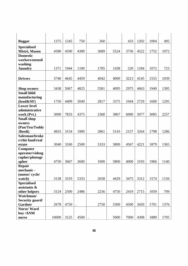
90
Beggar 1375 1245 750 260 . 433 1202 1004 495
Specialised Mistri, Mason 4580 4590 4389 3689 5524 3736 4522 1752 1072 Domestic workers/utensil washing /laundry 1371 1944 1100 1785 1438 520 1184 1072 723
Drivers 3740 4645 4459 4042 4000 3213 4145 1555 1039
Shop owners 3438 5067 4825 5581 4095 2975 4663 1949 1395 Small hhld manufacturing (food&NF) 1750 4409 2040 2817 3375 1044 2729 1600 1295 Lower level administrative work (Pvt.) 3000 7833 4375 2360 3867 6000 5077 3085 2257 Small shop owners (Pan/Tea/Toddy/Beedi) 4833 3154 1900 2861 5143 2157 3264 1798 1286 Salesman/broker/chit fund/real estate 3040 3160 2500 5333 5800 4567 4221 1879 1365 Computer operator/videographer/photographer 4750 3667 2600 1000 5800 4000 3193 1966 1140 Repair mechanic - (motor/ cycle/ watch) 3138 3319 5333 2658 4429 3475 3312 1574 1156 Specialised assistants & other helpers 3124 2500 2486 2256 4750 2419 2715 1059 709 Watchman/ Security guard/ Gardner 2678 4750 . 2750 5300 4500 3420 1701 1376 Nurse/ Ward boy /ANM nurse 10000 3125 4500 . 5000 7000 4308 1889 1705

91
Shop assistants 2800 3669 2825 1688 4246 1838 2719 1885 1130 Jajmani activities Priest and Barber 3200 3643 0 700 5733 1633 3529 1587
Employee/ Job 3000 8778 5000 3000 . . 7154 2070
Government Teacher/ Doctor 7000
13188
29000 17233 13800 20000
17648 9425
Security forces & other gvt.middle level staff 11000
12550
19250 15167 14533 11625
14140 3784
Government peon & drivers 9692 7871 9734 9818 7025 10571 9037 3273
Municipality and gvt. sweepers 4250 4000 . 5000 4500 . 4400 2498
1620
Annex. Table 15 : Mean Per Capita Income and Expenditure in SMTs (in Rupees)
Mean Per Capita Income (MPCI)
Mean Per Capita Expenditure (MPCE)
Parbhani 1171 712 Bidar 2217 1665 Mansa 1365 651 Madhubani 1322 903 Jangaon 3426 2856 Pakur 1072 815 Total 1726 1219

92
Annex. Table 16: Distribution of SMT households by MPCE quintiles (in%) Parbhani Bidar Mansa Madhubani Jangaon Pakur Total
Col %
Row %
Col %
Row %
Col %
Row %
Col %
Row %
Col %
Row %
Col %
Row %
Col %
Row %
Lowest Quintile 36.3 45.8 7.7 9.7 37.6 27.3 9.0 6.5 1.7 0.9 20.0 9.7 19.9 100 Second Quintile 26.8 33.6 12.5 15.6 23.6 17.0 22.4 16.1 7.0 3.9 28.6 13.8 20.1 100 Third Quintile 16.0 20.0 19.4 24.4 18.2 13.1 33.7 24.2 9.9 5.5 26.2 12.7 20.0 100 Fourth Quintile 14.1 17.7 25.5 32.0 15.9 11.5 22.8 16.4 24.4 13.6 18.1 8.8 20.0 100 Fifth Quintile 6.8 8.5 34.9 43.9 4.8 3.5 12.2 8.8 57.0 31.9 7.1 3.5 20.0 100 Total 100.0 25.1 100.0 25.1 100.0 14.5 100.0 14.4 100.0 11.2 100.0 9.7 100.0 100
Annex Table 17: Material of roof in SMT households by MPCE quintiles (in %)
Thatch grass and tarpaulin
Asbestos and tin
Tiled and wooden
Cement and bricks Total
Col % Row %
Col %
Row %
Col %
Row %
Col %
Row %
Col %
Row %
Lowest Quintile 23.1 10.4 23.3 52.5 18.1 11.6 15.2 25.5 19.9 100.0 Second Quintile 22.6 10.1 21.8 48.7 25.0 15.9 15.2 25.3 20.1 100.0 Third Quintile 30.8 13.8 19.1 42.9 22.1 14.1 17.5 29.3 20.0 100.0 Fourth Quintile 16.4 7.4 19.7 44.2 22.1 14.1 20.6 34.3 20.0 100.0 Fifth Quintile 7.2 3.2 16.0 36.0 12.7 8.1 31.5 52.7 20.0 100.0 Total 100.0 9.0 100.0 44.9 100.0 12.7 100.0 33.4 100.0 100.0
Annex Table 18: Material of Floor in SMT households by MPCE quintiles (in %)
Earthen and semi earthen
Bricks and cement Chips, tiles and stone Total
Col % Row % Col % Row % Col % Row %
Col %
Row %
Lowest Quintile 29.2 62.7 20.5 20.8 8.9 16.4 19.9 100.0 Second 25.9 55.4 21.9 22.1 12.3 22.5 20.1 100.0
93
Quintile Third Quintile 20.9 44.7 20.3 20.5 18.9 34.8 20.0 100.0 Fourth Quintile 16.1 34.6 21.0 21.2 24.0 44.2 20.0 100.0 Fifth Quintile 7.9 16.9 16.4 16.6 36.0 66.5 20.0 100.0 Total 100.0 42.9 100.0 20.2 100.0 36.9 100.0 100.0
Annex Table 19: Material of walls in SMT households by MPCE quintiles (in %)
Straw, mud, bamboo, wood and tin
Bricks and tiled
Stone
Concrete
Total
Col %
Row %
Col %
Row %
Col %
Row %
Col %
Row %
Col %
Row %
Lowest Quintile 24.2 29.6 21.5 51.9 9.9 9.5 21.2 9.0 19.9 100 Second Quintile 25.8 31.5 19.9 47.6 13.3 12.6 19.6 8.3 20.1 100 Third Quintile 24.7 30.2 17.5 41.9 20.3 19.4 20.1 8.5 20.0 100 Fourth Quintile 16.8 20.5 19.6 47.0 24.9 23.7 20.7 8.8 20.0 100 Fifth Quintile 8.5 10.4 21.4 51.5 31.6 30.3 18.5 7.9 20.0 100 Total 100.0 24.4 100.0 48.0 100.0 19.1 100.0 8.5 100.0 100
Annex Table: 20 Main Source of Lighting in SMT households by MPCE quintiles (in%) Kerosene Electricity Total
Col % Row % Col % Row % Col % Row %
Lowest Quintile 13.7 11.6 21.2 88.4 19.9 100.0 Second Quintile 28.0 23.4 18.5 76.6 20.1 100.0 Third Quintile 29.4 24.7 18.1 75.3 20.0 100.0

94
Fourth Quintile 19.2 16.1 20.2 83.9 20.0 100.0 Fifth Quintile 9.6 8.1 22.1 91.9 20.0 100.0 Total 100.0 16.8 100.0 83.2 100.0 100.0
Annex Table 21:Space used for cooking in SMT households by MPCE quintiles (in%) Separate Kitchen Other Space Total Col % Row % Col % Row % Col % Row % Lowest Quintile 9.0 12.4 23.2 87.6 19.4 100.0 Second Quintile 13.6 18.0 22.5 82.0 20.1 100.0 Third Quintile 17.9 23.8 20.8 76.2 20.0 100.0 Fourth Quintile 23.2 30.5 19.2 69.5 20.2 100.0 Fifth Quintile 36.3 47.9 14.3 52.1 20.2 100.0 Total 100.0 26.7 100.0 73.3 100.0 100.0
Annex Table 22: Asset categories by MPCE quintiles (in % households)
Cat. 1:
Cat. 2:
Cat. 3
Cat. 4
Cat.5 Total
Col %
Row %
Col % Row %
Col %
Row %
Col %
Row %
Col %
Row %
Col %
Row %
Lowest Quintile 24.5 30.0 24.1 14.3 19.0 18.8 17.0 27.5 15.9 9.4 19.9 100.0 Second Quintile 25.6 30.9 27.7 16.1 16.4 15.9 17.4 27.6 16.3 9.4 20.3 100.0 Third Quintile 23.5 28.7 21.3 12.6 19.4 19.2 19.1 30.8 14.7 8.6 20.0 100.0 Fourth Quintile 14.3 17.6 21.3 12.7 20.1 20.0 22.5 36.5 22.3 13.2 19.9 100.0 Fifth Quintile 12.0 14.8 5.5 3.3 25.1 24.9 24.1 39.0 30.7 18.1 19.9 100.0 Total 100.0 24.5 100.0 11.8 100.0 19.7 100.0 32.3 100.0 11.7 100.0 100.0
95
Annex Table 23: Main source of drinking water in SMT households by MPCE Quintiles (in%)
Public (Well ,hand pump,
tube well, stand post)
Purchase Water
Piped water Supply
Private (Well, bore wells,
hand pump, tube well) Total
Col % Row % Col % Row %
Col %
Row %
Col % Row %
Col %
Row %
Lowest Quintile 19.2 48.4 5.0 2.5 20.1 9.7 26.2 39.4 19.9 100.0 Second Quintile 21.1 52.9 7.7 3.9 20.6 9.9 22.3 33.3 20.1 100.0 Third Quintile 23.0 57.6 11.4 5.8 17.2 8.3 18.9 28.3 20.0 100.0 Fourth Quintile 21.1 53.0 25.5 12.9 17.7 8.5 17.1 25.6 20.0 100.0 Fifth Quintile 15.6 39.3 50.5 25.6 24.4 11.8 15.5 23.3 20.0 100.0 Total 100.0 50.2 100.0 10.1 100.0 9.6 100.0 30.0 100.0 100.0
Annex Table 24: Main source of cooking fuel in SMT households by MPCE quintiles (in%)
Firewood ,leaves and
wood shavings
Coal , gobar gas ,cow dung and
agricultural waste Kerosene and Electric sigri LPG Total
Col %
Row % Col % Row %
Col %
Row %
Col %
Row %
Col %
Row %
Lowest Quintile 24.3 69.1 29.0 16.7 9.6 4.4 8.5 9.7 19.9 100.0 Second Quintile 23.8 67.1 27.4 15.6 11.2 5.1 10.7 12.2 20.1 100.0 Third Quintile 21.4 60.5 25.8 14.8 16.2 7.4 15.2 17.3 20.0 100.0 Fourth Quintile 19.2 54.1 12.9 7.4 23.4 10.6 24.4 27.9 20.0 100.0 Fifth Quintile 11.3 32.1 4.8 2.8 39.6 18.0 41.2 47.1 20.0 100.0 Total 100.0 56.6 100.0 11.4 100.0 9.1 100.0 22.9 100.0 100.0
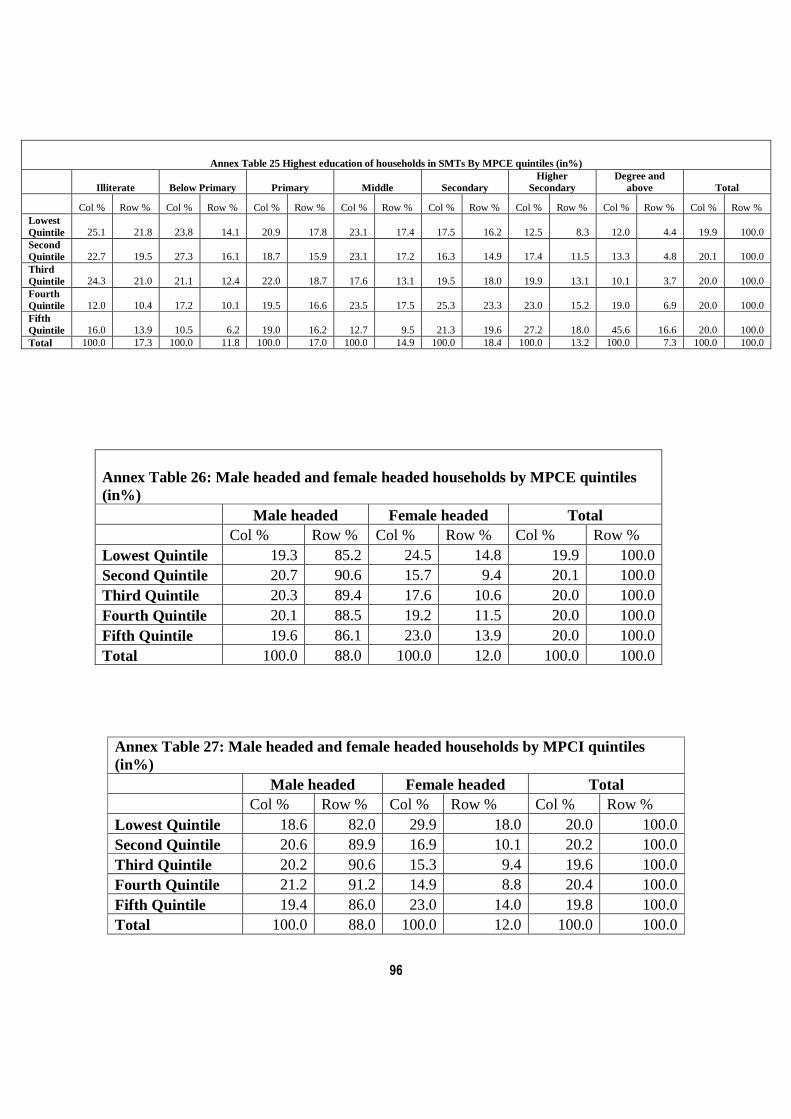
96
Annex Table 25 Highest education of households in SMTs By MPCE quintiles (in%)
Illiterate Below Primary Primary Middle Secondary Higher
Secondary Degree and
above Total
Col % Row % Col % Row % Col % Row % Col % Row % Col % Row % Col % Row % Col % Row % Col % Row % Lowest Quintile 25.1 21.8 23.8 14.1 20.9 17.8 23.1 17.4 17.5 16.2 12.5 8.3 12.0 4.4 19.9 100.0 Second Quintile 22.7 19.5 27.3 16.1 18.7 15.9 23.1 17.2 16.3 14.9 17.4 11.5 13.3 4.8 20.1 100.0 Third Quintile 24.3 21.0 21.1 12.4 22.0 18.7 17.6 13.1 19.5 18.0 19.9 13.1 10.1 3.7 20.0 100.0 Fourth Quintile 12.0 10.4 17.2 10.1 19.5 16.6 23.5 17.5 25.3 23.3 23.0 15.2 19.0 6.9 20.0 100.0 Fifth Quintile 16.0 13.9 10.5 6.2 19.0 16.2 12.7 9.5 21.3 19.6 27.2 18.0 45.6 16.6 20.0 100.0 Total 100.0 17.3 100.0 11.8 100.0 17.0 100.0 14.9 100.0 18.4 100.0 13.2 100.0 7.3 100.0 100.0
Annex Table 26: Male headed and female headed households by MPCE quintiles (in%) Male headed Female headed Total Col % Row % Col % Row % Col % Row % Lowest Quintile 19.3 85.2 24.5 14.8 19.9 100.0 Second Quintile 20.7 90.6 15.7 9.4 20.1 100.0 Third Quintile 20.3 89.4 17.6 10.6 20.0 100.0 Fourth Quintile 20.1 88.5 19.2 11.5 20.0 100.0 Fifth Quintile 19.6 86.1 23.0 13.9 20.0 100.0 Total 100.0 88.0 100.0 12.0 100.0 100.0
Annex Table 27: Male headed and female headed households by MPCI quintiles (in%) Male headed Female headed Total Col % Row % Col % Row % Col % Row % Lowest Quintile 18.6 82.0 29.9 18.0 20.0 100.0 Second Quintile 20.6 89.9 16.9 10.1 20.2 100.0 Third Quintile 20.2 90.6 15.3 9.4 19.6 100.0 Fourth Quintile 21.2 91.2 14.9 8.8 20.4 100.0 Fifth Quintile 19.4 86.0 23.0 14.0 19.8 100.0 Total 100.0 88.0 100.0 12.0 100.0 100.0

97
Annex Table 28: Households with and without disabled person in SMTs by MPCE quintiles (in%)
No disabled household member
Household having disabled member Total
Col % Row % Col % Row % Col % Row % Lowest Quintile 19.1 87.8 29.3 12.2 20.0 100.0 Second Quintile 19.7 89.7 24.9 10.3 20.2 100.0 Third Quintile 19.8 92.7 17.1 7.3 19.6 100.0 Fourth Quintile 21.2 95.0 12.2 5.0 20.4 100.0 Fifth Quintile 20.1 93.0 16.6 7.0 19.8 100.0 Total 100.0 91.7 100.0 8.3 100.0 100.0
Annex Table 29: Activity status of working and earning members in SMTs (in%) by MPCE quintiles
Lowest Quintile
Second Quintile
Third Quintile
Fourth Quintile
Fifth Quintile Total
Col %
Row %
Col %
Row %
Col %
Row %
Col %
Row %
Col %
Row %
Col %
Row %
Self Employed - Employer 0.1 1.0 2.0 17.2 1.2 9.1 2.7 22.2 7.9 50.5 2.5 100.0 Own account worker 25.3 21.8 23.4 20.4 25.0 19.6 24.4 20.2 27.8 17.9 25.0 100.0 Regular Wage / Salaried / Worker 15.3 15.3 18.3 18.5 23.2 21.1 24.0 23.1 29.3 21.9 21.6 100.0 Household based piece rate work 3.7 13.5 5.9 22.3 7.0 23.6 7.7 27.5 4.7 13.1 5.8 100.0 Casual wage labour 46.9 27.7 43.1 25.8 35.5 19.0 33.0 18.7 20.0 8.8 36.6 100.0 Unpaid family labour 1.3 12.9 2.4 24.7 2.2 20.0 2.9 28.2 1.9 14.1 2.2 100.0 Retired - Pensioner/ Widow Pensioner 3.2 16.4 2.8 14.5 3.4 15.8 4.9 24.2 7.6 29.1 4.2 100.0 Rentier 0.4 37.5 0.1 12.5 0.6 50.0 0.2 100.0 Beggar 3.9 44.6 2.1 24.3 2.5 25.7 0.4 4.1 0.2 1.4 1.9 100.0 Total 100.0 21.6 100.0 21.9 100.0 19.6 100.0 20.8 100.0 16.1 100.0 100.0

98
Annex Table 30: Composition of occupations in SMTs (in %) of working members
Parbhani
Bidar Mansa Madhubani Jangaon Pakur Total
Col % Col % Col % Col % Col % Col %
Col %
Construction labour 32.9 12.9 9.8 9.4 0.3 10.1 15.7 Agricultural labour 10.7 3.8 4.8 1.1 4.6 5.1 Boot Polish & Cobbler 0.3 0.6 10.7 1.7 2.5 2.4 Brick Kiln worker 1.7 0.5 1.9 0.5 0.9 Headload workers 1.7 3.0 6.4 0.4 0.5 0.8 2.4 Agri and construction workers (any) 0.2 0.9 5.7 0.2 0.3 0.3 1.2 Factory labour 0.6 0.8 1.2 2.8 0.8 0.3 1.1 Other specalised casua labour (saw mill/ ara machine etc) 2.9 4.0 0.3 0.7 9.3 2.5 3.0 Rickshaw Pulling & cart pulling 2.2 1.6 1.5 6.4 0.8 7.9 3.0 Welders/carpenters/polishers/fabricator/electricians 0.5 3.4 1.4 0.6 2.7 0.8 1.6 Waiter/ Hotel labour/ catering labour/Cook 4.7 4.7 0.2 3.1 1.4 1.1 3.1 Animal husbandry and fishing 0.1 0.1 0.5 2.2 0.8 2.8 0.8 Traditional Artisans (goldsmith/kitemaker/weaver/bidri work) 0.2 2.3 0.2 0.9 3.3 0.6 1.1 Painter 1.5 0.9 4.6 0.6 3.3 1.1 1.9 Teacher & Librarian (Pvt.) 0.1 1.3 1.8 1.6 2.5 1.0 Higher professional and technical services (Engineer&Doctor) 0.3 0.3 0.7 1.4 0.4 Vegetables, fruits, fish and poultry hawkers and vendors 1.7 3.3 0.5 6.3 1.9 1.4 2.5 Other food & NF vendors 0.8 3.1 0.7 4.4 1.1 1.1 1.9 Small businesses owners/contractor/ supplier/supervisor 0.5 1.0 0.3 0.7 1.9 0.6 0.8

99
Beedi making and garland making 1.7 0.6 0.7 12.0 24.7 4.3 Rag picker & scrap worker 1.7 2.8 19.1 0.9 0.3 4.3 Auto Driver 3.7 3.4 4.6 2.2 Tailoring 1.4 2.8 1.2 7.6 6.0 1.1 3.0 Sweepers (Pvt. ) 0.1 0.2 1.5 1.1 0.5 0.6 0.6 Beggar 0.8 7.5 0.3 0.2 0.8 2.1 Specialised Mistri, Mason 5.0 3.5 1.5 4.2 5.7 2.0 3.8 Domestic workers/utensil washing /laundry 5.1 1.0 3.1 2.4 2.2 10.4 3.7 Drivers 2.5 3.6 2.9 2.2 3.8 2.2 2.9 Shop owners 4.1 6.1 3.4 11.4 5.7 3.4 5.6 Small hhld manufacturing (food&NF) 0.4 1.3 1.7 2.2 2.7 2.5 1.5 Lower level administrative work (Pvt.) 0.1 1.0 0.7 0.9 1.6 0.3 0.7 Small shop owners (Pan/Tea/Toddy/Beedi) 0.6 1.5 0.5 4.2 1.9 2.0 1.6 Salesman/broker/chit fund/real estate 0.5 1.7 0.3 1.7 2.5 0.8 1.2 Computer operator/videographer/photographer 0.2 0.3 0.5 0.7 0.5 0.3 0.4 Repair mechanic - (motor/ cycle/ watch) 1.3 3.1 0.5 3.5 1.9 1.1 2.0 Specialised assistants & other helpers 1.7 0.5 1.2 1.7 0.5 4.2 1.5 Watchman/ Security guard/ Gardner 1.8 0.7 0.4 0.8 0.3 0.8 Nurse/ Ward boy /ANM nurse 0.1 0.9 0.3 0.3 0.3 0.4 Shop assistants 0.6 3.0 6.9 7.6 3.5 2.2 3.6 Jajmani activities Priest and Barber 0.6 0.8 0.2 0.2 1.6 0.8 0.7 Employee/ Job 0.1 1.0 0.2 0.4 0.4 Government Teacher/ Doctor 0.1 0.9 0.9 0.6 0.8 0.3 0.6 Security forces & other gvt.middle level staff 0.2 0.7 0.7 0.6 1.6 1.1 0.7

100
Government peon & drivers 1.3 2.0 1.5 0.6 1.1 2.0 1.4 Municipality and gvt. sweepers 0.4 0.1 0.2 1.1 0.3 Total 100.0 100.0 100.0 100.0 100.0 100.0 100.0
Annex Table 31: Minimum, mean and maximum values of MPCE quintiles (in Rupees) Minimum Mean Maximum Lowest Quintile 0 320 439 Second Quintile 440 529 620 Third Quintile 623 736 873 Fourth Quintile 874 1088 1400 Fifth Quintile 1403 3428 25850
Annex. Table 32: Distribution of SMT households by MPCI quintiles (in%) Parbhani Bidar Mansa Madhubani Jangaon Pakur Total
Col %
Row %
Col %
Row %
Col %
Row %
Col %
Row %
Col %
Row %
Col %
Row %
Col %
Row %
Lowest Quintile 21.1 26.6 9.5 12.0 26.4 19.2 24.7 17.8 3.3 1.8 46.7 22.6 20.0 100 Second Quintile 25.7 32.0 14.5 18.1 24.2 17.4 23.4 16.7 9.1 5.0 22.4 10.8 20.2 100 Third Quintile 20.9 26.8 21.1 27.1 21.3 15.8 21.8 16.0 12.4 7.1 14.8 7.3 19.6 100 Fourth Quintile 23.9 29.3 23.3 28.7 17.2 12.2 17.3 12.2 24.8 13.5 8.6 4.1 20.4 100 Fifth Quintile 8.4 10.7 31.6 40.0 10.8 7.9 12.8 9.3 50.4 28.4 7.6 3.7 19.8 100 Total 100.0 25.1 100.0 25.1 100.0 14.5 100.0 14.4 100.0 11.2 100.0 9.7 100.0 100

101
Annex Table 33: Households with and without disabled person in SMTs by MPCE quintiles (in%)
No disabled household member
Household having disabled member Total
Col % Row % Col % Row % Col % Row % Lowest Quintile 19.6 90.0 23.8 10.0 19.9 100.0 Second Quintile 19.7 90.1 23.8 9.9 20.1 100.0 Third Quintile 20.1 92.2 18.8 7.8 20.0 100.0 Fourth Quintile 20.2 92.4 18.2 7.6 20.0 100.0 Fifth Quintile 20.4 93.5 15.5 6.5 20.0 100.0 Total 100.0 91.7 100.0 8.3 100.0 100.0
Annex Table 34: Mean per capita income and mean per capita expenditure (in Rupees)
MPC Expenditure
MPC Income
Mean Mean Construction labour 730 1328 Agricultural labour 631 1350 Boot Polish & Cobbler 500 852 Brick Kiln worker 641 1905 Headload workers 731 1307 Agri and construction workers (any) 926 1295 Factory labour 956 1606 Other specalised casua labour (saw mill/ ara machine etc) 1076 1721 Rickshaw Pulling & cart pulling 741 1152 Welders/carpenters/polishers/fabricator/electricians 1388 1804 Waiter/ Hotel labour/ catering labour/Cook 877 1339 Animal husbandry and fishing 914 1371 Traditional Artisans (goldsmith/kitemaker/weaver/bidri work) 1847 2009 Painter 758 1409 Teacher & Librarian (Pvt.) 2497 3742 Higher professional and technical services (Engineer&Doctor) 2021 4344 Vegetables, fruits, fish and poultry hawkers and 1193 1769
102
vendors Other food & NF vendors 1174 1926 Small businesses owners/contractor/ supplier/supervisor 2237 2878 Beedi making and garland making 941 1169 Rag picker & scrap worker 630 1096 Auto Driver 1188 1822 Tailoring 1153 1571 Sweepers (Pvt. ) 915 1237 Beggar 495 1004 Specialised Mistri, Mason 1072 1752 Domestic workers/utensil washing /laundry 723 1072 Drivers 1039 1555 Shop owners 1395 1949 Small hhld manufacturing (food&NF) 1295 1600 Lower level administrative work (Pvt.) 2257 3085 Small shop owners (Pan/Tea/Toddy/Beedi) 1286 1798 Salesman/broker/chit fund/real estate 1365 1879 Computer operator/videographer/photographer 1140 1966 Repair mechanic - (motor/ cycle/ watch) 1156 1574 Specialised assistants & other helpers 709 1059 Watchman/ Security guard/ Gardner 1376 1701 Nurse/ Ward boy /ANM nurse 1705 1889 Shop assistants 1130 1885 Jajmani activities Priest and Barber 1106 1587 Employee/ Job 1312 2070 Government Teacher/ Doctor 3493 9425 Security forces & other gvt.middle level staff 1773 3784 Government peon & drivers 1868 3273 Municipality and gvt. sweepers 1743 2498 Total 1017 1620

103
Annex Table 35: Occupations of working and earning members in SMTs (in%) by MPCI quintiles
Lowest Quintile
Second Quintile
Third Quintile
Fourth Quintile
Fifth Quintile
Total
Col %
Row %
Col %
Row %
Col %
Row %
Col %
Row %
Col %
Row %
Col %
Row %
Construction labour 18.4 25.0 14.9 20.5 19.2 26.
0 15.
6 21.
8 5.0 6.7 14.6 100
Agricultural labour 3.3 24.6 2.6 19.3 2.6 19.
3 2.5 19.
3 2.4 17.
5 2.7 100
Boot Polish & Cobbler 5.0 38.9 4.4 35.2 2.6 20.
4 0.7 5.6 2.5 100
Brick Kiln worker 0.7 23.1 0.5 15.4 0.7 23.
1 0.5 15.
4 0.7 23.
1 0.6 100
Headload workers 2.4 20.8 4.0 35.4 2.4 20.
8 1.6 14.
6 1.0 8.3 2.3 100 Agri and construction workers (any) 2.6 33.3 1.6 21.2 1.0
12.1 1.6
21.2 1.0
12.1 1.5 100
Factory labour 0.5 7.4 1.4 22.2 1.7 25.
9 1.6 25.
9 1.2 18.
5 1.3 100 Other specalised casua labour (saw mill/ ara machine etc) 2.1 14.5 2.3 16.1 2.9
19.4 3.4
24.2 3.8
25.8 2.9 100
Rickshaw Pulling & cart pulling 5.9 29.8 5.6 28.6 4.3
21.4 2.5
13.1 1.4 7.1 3.9 100
Welders/carpenters/polishers/fabricator/electricians 0.9 9.8 2.1 22.0 1.2
12.2 3.0
31.7 2.4
24.4 1.9 100
Waiter/ Hotel labour/ catering labour/Cook 4.0 27.4 3.5 24.2 2.6
17.7 2.7
19.4 1.7
11.3 2.9 100
Animal husbandry and fishing 0.7 21.4 0.5 14.3 0.5
14.3 0.9
28.6 0.7
21.4 0.7 100
Traditional Artisans (goldsmith/kitemaker/weaver/bidri work) 0.5 6.9 0.2 3.4 1.7
24.1 1.8
27.6 2.6
37.9 1.4 100
Painter 2.1 18.8 2.6 22.9 2.4 20.
8 3.0 27.
1 1.2 10.
4 2.3 100
Teacher & Librarian (Pvt.) 0.7 11.5 0.5 7.7 1.0 15.
4 1.4 23.
1 2.6 42.
3 1.2 100 Higher professional and technical services (Engineer&Doctor) 0.2 7.7 0.7
23.1 2.1
69.2 0.6 100
Vegetables, fruits, fish and poultry hawkers and vendors 2.6 18.3 3.5 25.0 2.1
15.0 2.7
20.0 3.1
21.7 2.8 100

104
Other food & NF vendors 1.2 13.9 2.8 33.3 1.9 22.
2 1.1 13.
9 1.4 16.
7 1.7 100 Small businesses owners/contractor/ supplier/supervisor 0.5 7.7 0.5 7.7 1.8
30.8 3.3
53.8 1.2 100
Beedi making and garland making 3.3 48.3 1.2 17.2 0.2 3.4 0.5 6.9 1.7
24.1 1.4 100
Rag picker & scrap worker 5.4 41.1 2.3 17.9 2.6 19.
6 1.4 10.
7 1.4 10.
7 2.6 100
Auto Driver 1.7 12.1 2.8 20.7 2.4 17.
2 4.1 31.
0 2.6 19.
0 2.7 100
Tailoring 4.5 29.7 4.0 26.6 1.7 10.
9 1.8 12.
5 3.1 20.
3 3.0 100
Sweepers (Pvt. ) 1.9 53.3 0.5 13.
3 0.5 13.
3 0.7 20.
0 0.7 100
Beggar 2.1 32.1 2.1 32.1 0.7 10.
7 1.4 21.
4 0.2 3.6 1.3 100
Specialised Mistri, Mason 2.6 9.8 4.7 17.9 6.9 25.
9 5.7 22.
3 6.4 24.
1 5.3 100 Domestic workers/utensil washing /laundry 4.0 43.6 2.3 25.6 1.9
20.5 0.7 7.7 0.2 2.6 1.8 100
Drivers 2.8 14.5 4.0 20.5 4.5 22.
9 4.8 25.
3 3.3 16.
9 3.9 100
Shop owners 2.8 9.0 6.3 20.3 7.4 23.
3 7.3 24.
1 7.4 23.
3 6.2 100 Small hhld manufacturing (food&NF) 2.1 25.0 1.2 13.9 2.1
25.0 1.1
13.9 1.9
22.2 1.7 100
Lower level administrative work (Pvt.) 0.9 16.0 0.5 8.0 1.0
16.0 0.9
16.0 2.6
44.0 1.2 100
Small shop owners (Pan/Tea/Toddy/Beedi) 1.7 18.4 2.6 28.9 1.9
21.1 0.9
10.5 1.9
21.1 1.8 100
Salesman/broker/chit fund/real estate 0.5 7.4 1.2 18.5 1.9
29.6 0.7
11.1 2.1
33.3 1.3 100
Computer operator/videographer/photographer 0.5 22.2 0.2
11.1 0.9
44.4 0.5
22.2 0.4 100
Repair mechanic - (motor/ cycle/ watch) 1.4 13.6 3.3 31.8 2.4
22.7 1.6
15.9 1.7
15.9 2.1 100
Specialised assistants & other helpers 2.1 30.0 2.1 30.0 1.2
16.7 1.1
16.7 0.5 6.7 1.4 100
Watchman/ Security guard/ Gardner 0.5 9.1 0.7 13.6 1.0
18.2 2.1
40.9 1.0
18.2 1.0 100
Nurse/ Ward boy /ANM nurse 0.5 20.0 0.5 20.0 0.2
10.0 0.5
20.0 0.7
30.0 0.5 100
Shop assistants 1.7 10.1 2.1 13.0 4.0 24. 5.5 34. 2.9 17. 3.2 100
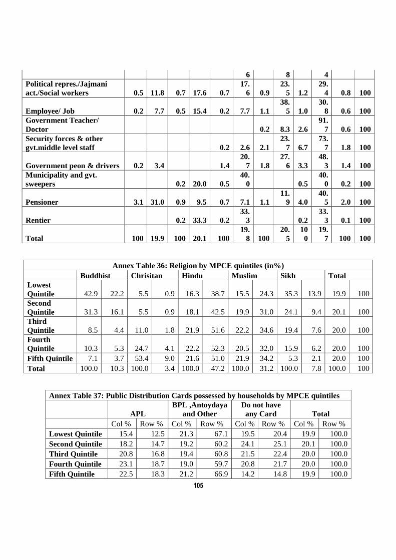
105
6 8 4 Political repres./Jajmani act./Social workers 0.5 11.8 0.7 17.6 0.7
17.6 0.9
23.5 1.2
29.4 0.8 100
Employee/ Job 0.2 7.7 0.5 15.4 0.2 7.7 1.1 38.
5 1.0 30.
8 0.6 100 Government Teacher/ Doctor 0.2 8.3 2.6
91.7 0.6 100
Security forces & other gvt.middle level staff 0.2 2.6 2.1
23.7 6.7
73.7 1.8 100
Government peon & drivers 0.2 3.4 1.4 20.
7 1.8 27.
6 3.3 48.
3 1.4 100 Municipality and gvt. sweepers 0.2 20.0 0.5
40.0 0.5
40.0 0.2 100
Pensioner 3.1 31.0 0.9 9.5 0.7 7.1 1.1 11.
9 4.0 40.
5 2.0 100
Rentier 0.2 33.3 0.2 33.
3 0.2 33.
3 0.1 100
Total 100 19.9 100 20.1 100 19.
8 100 20.
5 100
19.7 100 100
Annex Table 36: Religion by MPCE quintiles (in%) Buddhist Chrisitan Hindu Muslim Sikh Total Lowest Quintile 42.9 22.2 5.5 0.9 16.3 38.7 15.5 24.3 35.3 13.9 19.9 100 Second Quintile 31.3 16.1 5.5 0.9 18.1 42.5 19.9 31.0 24.1 9.4 20.1 100 Third Quintile 8.5 4.4 11.0 1.8 21.9 51.6 22.2 34.6 19.4 7.6 20.0 100 Fourth Quintile 10.3 5.3 24.7 4.1 22.2 52.3 20.5 32.0 15.9 6.2 20.0 100 Fifth Quintile 7.1 3.7 53.4 9.0 21.6 51.0 21.9 34.2 5.3 2.1 20.0 100 Total 100.0 10.3 100.0 3.4 100.0 47.2 100.0 31.2 100.0 7.8 100.0 100
Annex Table 37: Public Distribution Cards possessed by households by MPCE quintiles
APL BPL ,Antoydaya
and Other Do not have any Card Total
Col % Row % Col % Row % Col % Row % Col % Row % Lowest Quintile 15.4 12.5 21.3 67.1 19.5 20.4 19.9 100.0 Second Quintile 18.2 14.7 19.2 60.2 24.1 25.1 20.1 100.0 Third Quintile 20.8 16.8 19.4 60.8 21.5 22.4 20.0 100.0 Fourth Quintile 23.1 18.7 19.0 59.7 20.8 21.7 20.0 100.0 Fifth Quintile 22.5 18.3 21.2 66.9 14.2 14.8 19.9 100.0

106
Annex Table 38: Public Distribution Cards possessed by households by MPCI quintiles (in%)
APL
BPL ,Antoydaya and Other
Do not have any
Card Total Lowest Quintile 16.5 19.7 23.5 20.0 Second Quintile 17.7 19.5 24.1 20.2 Third Quintile 19.9 20.4 16.8 19.6 Fourth Quintile 19.9 20.2 21.7 20.4 Fifth Quintile 25.9 20.2 13.9 19.8 Total 100 100 100 100
Annex Table 39: Minimum, mean and maximum values of MPCE and MPCI by quintiles (in Rs.)
Monthly Per Capita Income Monthly Per Capita Expenditure
Minimum Mean Maximum Minimum Mean Maximum
Lowest Quintile 0 499 675 0 320 439
Second Quintile 678 808 950 440 529 620
Third Quintile 960 1110 1329 623 736 873
Fourth Quintile 1333 1651 2000 874 1088 1400
Fifth Quintile 2025 4581 39000 1403 3428 25850

107
Annexure 6: List of Supervisors and Field Investigators
BIDAR
Baswaraj, S.
Hidayath
Putraj
Raghavender, S.
Raj Kumar
Sudhakar
Veeresh
PARBHANI
Ajay Panpat
Lata Bhansode
Ravidas Murlidhar
Rohan Kamble
Rohidas Gadhge
S.V. Sutare
MANSA
Gurpreet Singh
Manpreet Singh
Rakesh Kumar
Surinder Kumar
Kriman K.
Yadu C.R
MADHUBANI
Ajit Kumar
Gautam Kumar
Manju Kumari
Ram Pramod Yadav
Vibhav Shankar Pandey
Vijay Prasad
JANGAON
G. Suresh
K.Raju
N. Kanna
R. Anil Kumar
S. Raghavendra
PAKUR
Amit Kumar
Devraj Baghchi
Ritu Gudia
Shyamaditya Singh Deo
Suman Kumari
Vibhav Shankar Pandey
Vijay Prasad