NREL is a national laboratory of the U.S. Department of Energy, Office of Energy Efficiency & Renewable Energy, operated by the Alliance for Sustainable Energy, LLC.

Contract No. DE-AC36-08GO28308

Naval Station Newport Wind Resource Assessment A Study Prepared in Partnership with the Environmental Protection Agency for the RE-Powering America’s Land Initiative: Siting Renewable Energy on Potentially Contaminated Land and Mine Sites, and The Naval Facilities Engineering Service Center

Robi Robichaud, Jason Fields, and Joseph Owen Roberts

Technical Report NREL/TP-6A20-52801 February 2012

NREL is a national laboratory of the U.S. Department of Energy, Office of Energy Efficiency & Renewable Energy, operated by the Alliance for Sustainable Energy, LLC.

National Renewable Energy Laboratory 1617 Cole Boulevard Golden, Colorado 80401 303-275-3000 • www.nrel.gov

Contract No. DE-AC36-08GO28308

Naval Station Newport Wind Resource Assessment A Study Prepared in Partnership with the Environmental Protection Agency for the RE-Powering America’s Land Initiative: Siting Renewable Energy on Potentially Contaminated Land and Mine Sites, and The Naval Facilities Engineering Service Center

Robi Robichaud, Jason Fields, and Joseph Owen Roberts

Prepared under Task No. WFD5.1000

Technical Report NREL/TP-6A20-52801 February 2012

NOTICE

This report was prepared as an account of work sponsored by an agency of the United States government. Neither the United States government nor any agency thereof, nor any of their employees, makes any warranty, express or implied, or assumes any legal liability or responsibility for the accuracy, completeness, or usefulness of any information, apparatus, product, or process disclosed, or represents that its use would not infringe privately owned rights. Reference herein to any specific commercial product, process, or service by trade name, trademark, manufacturer, or otherwise does not necessarily constitute or imply its endorsement, recommendation, or favoring by the United States government or any agency thereof. The views and opinions of authors expressed herein do not necessarily state or reflect those of the United States government or any agency thereof.

Available electronically at http://www.osti.gov/bridge

Available for a processing fee to U.S. Department of Energy and its contractors, in paper, from:

U.S. Department of Energy Office of Scientific and Technical Information P.O. Box 62 Oak Ridge, TN 37831-0062 phone: 865.576.8401 fax: 865.576.5728 email: mailto:reports@adonis.osti.gov

Available for sale to the public, in paper, from:

U.S. Department of Commerce National Technical Information Service 5285 Port Royal Road Springfield, VA 22161 phone: 800.553.6847 fax: 703.605.6900 email: orders@ntis.fedworld.gov online ordering: http://www.ntis.gov/help/ordermethods.aspx

Cover Photos: (left to right) PIX 16416, PIX 17423, PIX 16560, PIX 17613, PIX 17436, PIX 17721

Printed on paper containing at least 50% wastepaper, including 10% post consumer waste.

iii

Acknowledgments

The wind resource analysis and assessment presented in this report was sponsored by the U.S. Environmental Protection Agency (EPA). The installation of the meteorological (met) tower at Coddington Point was sponsored by the Naval Facilities Engineering Service Center (NFESC) and implemented by the National Renewable Energy Laboratory (NREL). The installation of the met tower at Tank Farm #4 was undertaken by NFESC. The Sonic detection and ranging (SODAR) unit is on loan to Naval Station (NAVSTA) Newport from the NREL, and the summary reports from SODAR were sponsored by NFESC. John Reichert, Energy Engineer at NAVSTA Newport, provided information regarding the electricity consumption and utility cost information. NREL staff members involved were Robi Robichaud, principal investigator, and Gail Mosey, NREL’s project lead for the EPA RE-Powering America’s Lands programs; Owen Roberts conducted the correlation assessment of the collected met tower data to a long-term reference station; and Jason Fields conducted the wind flow analysis and energy production estimates using weather data from the met towers.

iv

Executive Summary

The U.S. Environmental Protection Agency (EPA) launched the RE-Powering America’s Land: Siting Renewable Energy on Potentially Contaminated Land and Mine Sites initiative in September 2008. EPA and the U.S. Department of Energy’s National Renewable Energy Laboratory (NREL) are collaborating on a number of projects to evaluate the feasibility of siting renewable energy (RE) technologies on these potentially contaminated sites. This report focuses on the wind resource assessment campaign at Naval Station (NAVSTA) Newport in Newport, Rhode Island.

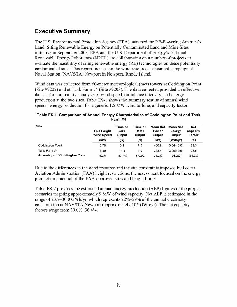
Wind data was collected from 60-meter meteorological (met) towers at Coddington Point (Site #9202) and at Tank Farm #4 (Site #9203). The data collected provided an effective dataset for comparative analysis of wind speed, turbulence intensity, and energy production at the two sites. Table ES-1 shows the summary results of annual wind speeds, energy production for a generic 1.5 MW wind turbine, and capacity factor.

Table ES-1. Comparison of Annual Energy Characteristics of Coddington Point and Tank Farm #4

Due to the differences in the wind resource and the site constraints imposed by Federal Aviation Administration (FAA) height restrictions, the assessment focused on the energy production potential of the FAA-approved sites and height limits.

Table ES-2 provides the estimated annual energy production (AEP) figures of the project scenarios targeting approximately 9 MW of wind capacity. Net AEP is estimated in the range of 23.7–30.0 GWh/yr, which represents 22%–29% of the annual electricity consumption at NAVSTA Newport (approximately 105 GWh/yr). The net capacity factors range from 30.0%–36.4%.

SiteHub Height

Wind Speed

Time at Zero

Output

Time at Rated Output

Mean Net Power Output

Mean Net Energy Output

Net Capacity

Factor(m/s) (%) (%) (kW) (kWh/yr) (%)

Coddington Point 6.79 6.1 7.5 438.9 3,844,637 29.3

Tank Farm #4 6.39 14.3 4.0 353.4 3,095,995 23.6Advantage of Coddington Point 6.3% -57.4% 87.2% 24.2% 24.2% 24.2%

v

Table ES-2. Annual Energy Production Figures for Approximately 9 MW of Wind at NAVSTA Newport

Overall, the wind resource at the selected sites at NAVSTA Newport is sufficient for a wind turbine project. There are a number of other factors to consider before turbine selection is undertaken, including cost, availability, constructability, and transportability. There are also a number of other factors still to be explored as the parameters of this project become more clearly defined, including financing, National Environmental Protection Act (NEPA), constructability, subsoil/foundations, impact on neighbors, and transportation planning and logistics.

There are a number of proposed tasks to continue to move this project forward, including:

• NAVSTA Newport to complete the NEPA evaluation already underway

• NREL/DNV to complete an electrical interconnection study

• Complete the economic feasibility study

• Complete the transportation and logistics study

• Complete the visual and sound impact study

• Develop a public information plan.

Characteristics Unit ~9 MW ScenarioWTG* Manufacturer Siemens GE Vestas Vestas Nordex REPower AlstomWTG Model # 2.3 MW XLE 100 V100 V112 N100 MM100 ECO 110WTG Capacity MW 2.3 1.6 1.8 3.0 2.5 1.8 3.0WTG Hub Height m 80 80 80 80 80 80 80WTG Rotor Diameter m 101 100 100 112 100 100 110Array Size # 4 6 5 3 4 5 3Site Capacity MW 9.20 9.60 9.00 9.00 10.00 9.00 9.00Ideal Yield GWh/yr 31.27 37.33 34.70 30.19 32.08 35.11 28.19Gross AEP Central Estimate GWh/yr 30.79 35.65 33.50 29.56 31.57 33.89 27.59Net AEP Central Estimate GWh/yr 25.74 30.05 28.35 25.36 26.44 28.73 23.67Net Capacity Factor % 31.93 35.73 35.95 32.17 30.18 36.44 30.02*WTG = Wind Turbine Generator; AEP = Annual Energy Production

vi

Table of Contents Acknowledgments ...................................................................................................................................... iii Executive Summary ................................................................................................................................... iv Table of Contents ....................................................................................................................................... vi List of Figures ........................................................................................................................................... viii List of Tables ................................................................................................................................................ x 1 Introduction ........................................................................................................................................... 1 2 Location ................................................................................................................................................. 2 3 Wind Resource Assessment Campaign ............................................................................................. 4

3.1 Wind Resource Assessment Activities at NAVSTA Newport ......................................4 4 Site Characterization ............................................................................................................................ 5 5 Wind in Rhode Island ............................................................................................................................ 7 6 Instrumentation and Equipment .......................................................................................................... 9

6.1 Meteorological Towers ..................................................................................................9 6.2 Site Summary ...............................................................................................................11 6.3 SODAR Systems ..........................................................................................................11 6.4 MiniSODAR ................................................................................................................12

7 Data Recovery and Validation ........................................................................................................... 13 7.1 Data Analysis ...............................................................................................................15

8 Wind Resource Assessment Summary ............................................................................................ 16 8.1 Wind Resource Characterization .................................................................................16 8.2 Measuring Power in the Wind .....................................................................................16 8.3 NAVSTA Newport Wind Speed Variability ...............................................................16 8.4 NAVSTA Newport Monthly Box Plot Statistics ..........................................................17 8.5 NAVSTA Newport Seasonal Wind Profile .................................................................18 8.6 NAVSTA Newport Diurnal Wind Profile ...................................................................19 8.7 NAVSTA Newport Wind Direction Data ....................................................................22 8.8 NAVSTA Newport Wind Frequency (Probability) Distribution .................................25 8.9 Vertical Wind Shear .....................................................................................................27 8.10 Turbulence Intensity ....................................................................................................33 8.11 Energy Production Potential of Coddington Point and Tank Farm #4 ........................36

9 MiniSODAR Data ................................................................................................................................. 39 10 Long-Term Data Adjustment .............................................................................................................. 40

10.1 Long-Term Datasets.....................................................................................................40 11 Energy Production Estimates ............................................................................................................ 45

11.1 Wind Turbines Modeled ..............................................................................................45 11.2 Site Layout ...................................................................................................................45 11.3 Energy Production Loss Factors ..................................................................................48 11.4 Site Climatology ..........................................................................................................50 11.5 Wake Modeling and Energy Production ......................................................................51

12 Conclusions and Recommendations ................................................................................................ 53 12.1 Conclusions ..................................................................................................................53 12.2 Recommendations ........................................................................................................54

vii

Appendix A. Met Tower Sensors .............................................................................................................. 55 Appendix B. Turbulence Analysis ........................................................................................................... 58 Appendix C. Additional Site Information ................................................................................................ 62

viii

List of Figures

Figure 1. Location of NAVSTA Newport, Rhode Island ................................................................2 Figure 2. Topographical map of NAVSTA Newport showing possible wind development

sites. .................................................................................................................................3 Figure 3. Image of the NAVSTA Newport base with view to the north .........................................6 Figure 4. Rhode Island wind speed map at 80 m .............................................................................8 Figure 5. Map of NAVSTA Newport with met tower locations....................................................10 Figure 6. Wind data at 58 m at Coddington Point, May–June 2010 ..............................................17 Figure 7. Boxplot of Coddington Point, April 1, 2010, to March 31, 2011...................................17 Figure 8. Boxplot of Tank Farm #4, April 1, 2010, to March 31, 2011 ........................................18 Figure 9. Seasonal wind speed profile at Coddington Point, April 1, 2010, to March 31,

2011 ...............................................................................................................................18 Figure 10. Seasonal wind speed profile at Tank Farm #4, April 1, 2010, to March 31,

2011 ...............................................................................................................................19 Figure 11. Diurnal profile of the wind speed at Coddington Point, April 1, 2010, to March

31, 2011 .........................................................................................................................20 Figure 12. Diurnal profile of the wind speed at Tank Farm #4, April 1, 2010, to March

31, 2011 .........................................................................................................................20 Figure 13. Monthly diurnal profile of the wind speed at Coddington Point, April 1, 2010,

to March 31, 2011 .........................................................................................................21 Figure 14. Monthly diurnal profile of the wind speed at Tank Farm #4, April 1, 2010, to

March 31, 2011 .............................................................................................................22 Figure 15. Wind frequency rose at Coddington Point and Tank Farm #4 at 58 m, April 1,

2010, to March 31, 2011 ...............................................................................................23 Figure 16. Total wind energy rose at Coddington Point and Tank Farm #4 at 58 m, April

1, 2010, to March 31, 2011 ...........................................................................................24 Figure 17. Total wind energy rose at Coddington Point by month at 58 m, April 1, 2010,

to March 31, 2011 .........................................................................................................24 Figure 18. Total wind energy rose at Tank Farm #4 by month at 58 m, April 1, 2010, to

March 31, 2011 .............................................................................................................25 Figure 19. Wind frequency distribution for Coddington Point at 58 m, April 1, 2010, to

March 31, 2011 .............................................................................................................26 Figure 20. Wind frequency distribution for Tank Farm #4 at 58 m, April 1, 2010, to

March 31, 2011 .............................................................................................................26 Figure 21. Vertical wind shear profile at Coddington Point and Tank Farm #4 at 58 m,

April 1, 2010, to March 31, 2011 ..................................................................................31 Figure 22. Daily wind shear profile by month at Coddington Point, April 1, 2010, to

March 31, 2011 .............................................................................................................32 Figure 23. Daily wind shear profile by month at Tank Farm #4, April 1, 2010, to March

31, 2011 .........................................................................................................................32

ix

Figure 24. Representative and mean turbulence intensities for Coddington Point, April 1, 2010, to March 31, 2011 ...............................................................................................34

Figure 25. Turbulence intensity for Coddington Point at 58 m, April 1, 2010, to March 31, 2011 .........................................................................................................................35

Figure 26. Turbulence intensity for Tank Farm #4 at 58 m, April 1, 2010, to March 31, 2011 ...............................................................................................................................36

Figure 27. Monthly data recovery rates at Newport Airport, December 1998–March 2011 .........41 Figure 28. Corrected long-term annual mean wind speeds and overall mean annual wind

speed at Newport Airport, January 1, 1999, to March 31, 2011 ...................................42 Figure 29. Collected data at Coddington Point versus collected and long-term data at

Newport Airport ............................................................................................................42 Figure 30. Comparison of Coddington Point data with the MCP adjusted wind data, July

1, 2009, to March 31, 2011 ...........................................................................................44 Figure 31. Wind speed map of NAVSTA Newport based on data collected on site .....................51 Figure A-1. Anemometer #40C NRG Systems (item 1899) ..........................................................55 Figure A-2. Wind vane NRG Systems #200P (item 1904) ............................................................56 Figure A-3. Boom, side, 1.53m (60.5"), galvanized, with clamps (item: 3390) ............................56 Figure A-4. 50m and 60m XHD Tower configuration ..................................................................57 Figure B-1. Turbulence intensity by direction at Coddington Point ..............................................58 Figure B-2. Turbulence intensity by direction at Tank Farm #4 ...................................................58 Figure B-3. Diurnal turbulence intensity at 58 m at Coddington Point .........................................59 Figure B-4. Diurnal turbulence intensity at 58 m at Tank Farm #4 ...............................................59 Figure B-5. Seasonal turbulence intensity at 58 m at Coddington Point .......................................60 Figure B-6. Seasonal turbulence intensity at 58 m at Tank Farm #4 .............................................60 Figure B-7. Turbulence intensity vs. wind speed at Coddington Point .........................................61 Figure B-8. Turbulence intensity vs. wind speed at Tank Farm #4 ...............................................61

x

List of Tables

Table ES-1. Comparison of Annual Energy Characteristics of Coddington Point and Tank Farm #4 ......................................................................................................................... iv

Table ES-2. Annual Energy Production Figures for Approximately 9 MW of Wind at NAVSTA Newport .........................................................................................................v

Table 1. Sensors, Heights, and Orientations at Coddington Point ...................................................9 Table 2. Sensors, Heights, and Orientations at Tank Farm #4 ........................................................9 Table 3. Site Summaries of the Met Tower Sites ..........................................................................11 Table 4. Log of MiniSODAR Locations, February 2010–August 2011........................................12 Table 5. Dataset Recovery Rates for Coddington Point, April 1, 2010, to March 31, 2011 .........13 Table 6. Dataset Recovery Rates for Tank Farm #4, April 1, 2010, to March 31, 2011 ...............14 Table 7. Surface Roughness Lengths and Descriptions .................................................................28 Table 8. Power Law Exponent and Surface Roughness Length for Coddington Point,

April 1, 2010, to March 31, 2011 ..................................................................................29 Table 9. Power Law Exponent and Surface Roughness Length for Tank Farm #4,

April 1, 2010, to March 31, 2011 ..................................................................................30 Table 10. IEC Wind Turbine Classes, Ratings, and Characteristics of Turbulence

Intensity .........................................................................................................................34 Table 11. FAA-Permitted Heights and Turbine Dimensions.........................................................37 Table 12. Coddington Point Energy Production with Low Wind Speed Class C Turbine ............37 Table 13. Tank Farm #4 Energy Production with Medium Wind Speed Class B Turbine ...........38 Table 14. Newport Airport and Coddington Point Data Adjusted to Long-Term Trends .............43 Table 15. Wind Turbine Specifications Used in Modeling ...........................................................45 Table 16. FAA-Approved Heights at Each Site.............................................................................46 Table 17. Total Wind Turbine Heights Compared to FAA-Approved Heights ............................47 Table 18. Recommended Turbine Per Project Size Parameter of 9 MW ......................................48 Table 19. Site Production Annual Loss Factors for the 9 MW Scenario .......................................50 Table 20. Annual Energy Production Figures for One Wind Turbine at Each of the Seven

Sites at NAVSTA Newport ...........................................................................................52 Table 21. Annual Energy Production Figures for Approximately 9 MW of Wind at

NAVSTA Newport .......................................................................................................52 Table 22. Annual Energy Production Figures for Approximately 9 MW of Wind at

NAVSTA Newport .......................................................................................................53 Table C-1. FAA-Approved Heights for Each Site .........................................................................62

1

1 Introduction

In 2008, the U.S. Environmental Protection Agency (EPA) launched the RE-Powering America’s Land initiative to encourage the development of renewable energy (RE) on potentially contaminated land and mine sites. As part of this effort, EPA is collaborating with the U.S. Department of Energy’s (DOE’s) National Renewable Energy Laboratory (NREL) to evaluate RE options at Naval Station (NAVSTA) Newport in Newport, Rhode Island.

EPA has been involved with NAVSTA Newport as there are multiple contaminated areas that pose a threat to human health and the environment. The base was designated a superfund site on the National Priorities List in 1989. NAVSTA Newport is committed to working toward reducing the base’s dependency on fossil fuels, decreasing its carbon footprint, and implementing RE projects where feasible. EPA Region 1 and NAVSTA Newport have engaged NREL to investigate the RE options for the base.

The Naval Facilities Engineering Service Center (NFESC) partnered with NREL in February 2009 to investigate the potential for wind energy generation at a number of Naval and Marine bases on the East Coast. NAVSTA Newport was one of several bases chosen for a detailed, site-specific wind resource investigation. NAVSTA Newport, in conjunction with NREL and NFESC, has been actively engaged in assessing the wind resource through several ongoing efforts.

This report focuses on the wind resource assessment, the estimated energy production of wind turbines, and a survey of potential wind turbine options based upon the site-specific wind resource.

2

2 Location

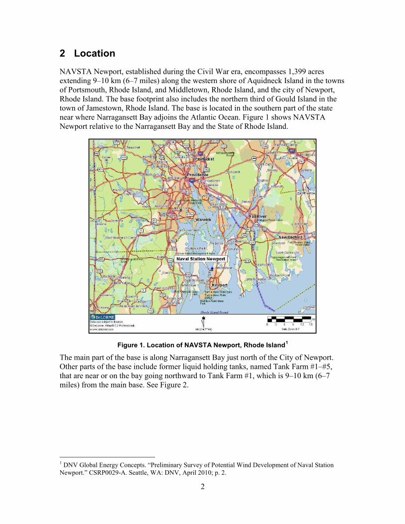
NAVSTA Newport, established during the Civil War era, encompasses 1,399 acres extending 9–10 km (6–7 miles) along the western shore of Aquidneck Island in the towns of Portsmouth, Rhode Island, and Middletown, Rhode Island, and the city of Newport, Rhode Island. The base footprint also includes the northern third of Gould Island in the town of Jamestown, Rhode Island. The base is located in the southern part of the state near where Narragansett Bay adjoins the Atlantic Ocean. Figure 1 shows NAVSTA Newport relative to the Narragansett Bay and the State of Rhode Island.

Figure 1. Location of NAVSTA Newport, Rhode Island1

The main part of the base is along Narragansett Bay just north of the City of Newport. Other parts of the base include former liquid holding tanks, named Tank Farm #1–#5, that are near or on the bay going northward to Tank Farm #1, which is 9–10 km (6–7 miles) from the main base. See Figure 2.

1 DNV Global Energy Concepts. “Preliminary Survey of Potential Wind Development of Naval Station Newport.” CSRP0029-A. Seattle, WA: DNV, April 2010; p. 2.

3

Figure 2. Topographical map of NAVSTA Newport showing possible wind development sites.2

Note: McAlister Point Landfill is included in the label for Tank Farm #5.

2 DNV Global Energy Concepts. “Preliminary Survey of Potential Wind Development of Naval Station Newport.” CSRP0029-A. Seattle, WA: DNV, April 2010; p. 3.

4

3 Wind Resource Assessment Campaign

The assessment characterized the wind resource for the entire base to identify the most promising sites. Primary wind characteristics of interest include:

• Wind speed at or close to proposed wind turbine sites

• Vertical wind shear factor (VWSF) to determine wind speeds at hub height

• Wind speed frequency distribution (aka probability distribution function)

• Turbulence intensity (TI) to determine turbine site suitability based upon standard International Electrotechnical Commission (IEC) classifications.

3.1 Wind Resource Assessment Activities at NAVSTA Newport The wind assessment campaign has been actively engaged in assessing the wind resource through several ongoing efforts and equipment, as follows:

• Coddington Point, Site #9202—60 m meteorological (met) tower installed and operational since July 29, 2009

• MiniSODAR unit installed and operational at Coddington Point since February 22, 2010

• Tank Farm #4, Site #9203—60 m met tower installed and operational since March 19, 2010.

The original wind assessment campaign called for two fixed met tower stations at or near the northern and southern ends of the base that would be installed for at least one year. However, the base, which extends roughly 6–7 miles north to south along a jagged coastline, has a topography that is not easily characterized. It includes hills rising quickly from the shore and areas that are densely populated with one- to four-story buildings. Different locations within the base will have different wind regimes due to topography and surface roughness. Wind regimes within the base vary according to topography, surface roughness, season, and time of day.

An Atmospheric Systems Corporation (ASC) mini sonic detection and ranging (miniSODAR) unit was added to enhance the analysis with measurements at heights up to twice as high as what met towers can readily provide. Met towers are stationary and not easily moved, whereas a miniSODAR has the advantage of being portable so that it can be used to characterize multiple sites.

5

4 Site Characterization

The main base terrain varies from generally flat to small hills in the 3–30 m (10–130 ft) range. The highest point on or adjacent to the main base is Miantonomi Hill (approximately 50 m or 165 ft) in Memorial Park. This hill can impede wind flow coming from the east or southeast and flowing toward Coddington Point or Coasters Harbor Island. The proposed locations for wind turbines are flat or are adjacent to smaller hills in the 3–10 m (10–35 ft) range.

The main base is populated with one- to four-story buildings. Taller buildings can cause turbulence even for utility-scale wind turbines when they are less than 400 m (approximately 1,300 ft) upwind. The one- to two-story buildings have minimal impact on utility-scale turbines. For wind turbines located on Coasters Harbor Island, Coddington Point, or along Coddington Cove, the buildings are expected to be the primary source of turbulence when winds are coming from the northwest or southwest.

The vegetation throughout the base is primarily deciduous with larger trees further inland and more grassy areas and smaller trees or bushes closer to the bay. The vegetation near the proposed turbine sites is not expected to represent a significant source of turbulence.

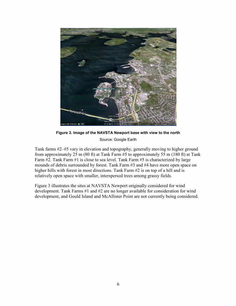
The sites with the highest wind speeds and lowest turbulence will be those along the western shores of Coasters Harbor Island and Coddington Point bordering the Narragansett Bay. These sites will have access to both the predominant northwestern winds and secondary southwestern winds across the smooth surface of the bay that. Figure 3 shows the fetch across the water to the northwest and southwest.

6

Figure 3. Image of the NAVSTA Newport base with view to the north

Source: Google Earth

Tank farms #2–#5 vary in elevation and topography, generally moving to higher ground from approximately 25 m (80 ft) at Tank Farm #5 to approximately 55 m (180 ft) at Tank Farm #2. Tank Farm #1 is close to sea level. Tank Farm #5 is characterized by large mounds of debris surrounded by forest. Tank Farm #3 and #4 have more open space on higher hills with forest in most directions. Tank Farm #2 is on top of a hill and is relatively open space with smaller, interspersed trees among grassy fields.

Figure 3 illustrates the sites at NAVSTA Newport originally considered for wind development. Tank Farms #1 and #2 are no longer available for consideration for wind development, and Gould Island and McAllister Point are not currently being considered.

7

5 Wind in Rhode Island

Wind maps provide a graphical estimation of the wind resource in an area but do not incorporate sufficient information to reliably estimate annual electricity generation at any specific point. Areas of varying vegetation (e.g., tall trees versus grassland or cropland), complex topographical features (e.g., ridges versus valleys or canyons versus mountains), and varying surface roughness (e.g., city skyscrapers versus flat or rolling farmland) are characterized by highly variable wind resources that are very site specific. Sites in close proximity to each other, but with the above variations, can represent different wind power densities. Wind maps are valuable for understanding, where strong winds merit further investigation with on-site wind monitoring stations. Wind maps are not, however, typically used to site large wind farms, because maps lack the micro-siting detail required to minimize the energy estimation uncertainty to the level required by financiers. On-site wind data collected for a period of 1–3 years is the industry norm to estimate wind turbine performance accurately. This study used recently collected on-site wind data for its analysis and energy production estimates.

The wind map for Rhode Island, shown in Figure 4, provides a context for the data analysis that follows. The wind map indicates NAVSTA Newport is in a region with an expected mean annual wind speed between 6.0–6.5 m/s (13.4–14.5 mph) at 80 m (262 ft). Some variation in wind speeds is expected depending upon access to wind across the bay and the proximity of hills, ravines, and buildings, for example.

8

Figure 4. Rhode Island wind speed map at 80 m3

3 Wind Powering America, DOE. "Rhode Island Wind Map and Resource Potential," Wind Powering America website, http://www.windpoweringamerica.gov/images/windmaps/ri_80m.jpg. Accessed July 26, 2011.

9

6 Instrumentation and Equipment

6.1 Meteorological Towers Met towers are temporary structures installed at or as close as possible to potential wind turbine sites to reduce the uncertainty of wind turbine energy production estimates. The towers may be 40–100 m (130–330 ft) tall, though 60–80 m (200–260 ft) is the most common for utility-scale wind turbine investigations. The met towers are usually configured with multiple anemometers, to measure the wind speed near the top of the tower and at 10–15 m (33–50 ft) intervals to a minimum height of 20–30 m (65–100 ft) above the ground. The met tower will also typically have two to three wind vanes to measure the wind direction at several heights.

At NAVSTA Newport, the met tower instrumentation consisted of an NRG 60 m XHD Tall Tower, six anemometers, two wind vanes, temperature sensor, barometric pressure sensor, and a data logger. The met towers were erected at Coddington Point (Site #9202) and at Tank Farm #4 (Site #9203). The met tower at Coddington Point was erected in July 2009 and was operational as of July 29, 2009. Table 1 summarizes details of the sensor configuration at Coddington Point. The information was taken from the Coddington Point commissioning report.4 Sensor and tower details are in Appendix A.

Table 1. Sensors, Heights, and Orientations at Coddington Point

The met tower at Tank Farm #4 was erected in March 2010 and was operational as of March 19, 2010. Table 2 summarizes details of the sensor configuration at Tank Farm #4. The information was taken from the Tank Farm #4 commissioning report.5

Table 2. Sensors, Heights, and Orientations at Tank Farm #4

4 DNV Commissioning Report for Site #9202, July 28, 2009. 5 DNV Commissioning Report for Site #9203, March 18, 2010.

cmcmcmcmcmcmcmcmcm 270

188270--

187275

Direction274

Boom lengthSensor mounting heightModel number Serial number Slope OffsetSensors: TypeVendor Name

Ch. #40C Anemometer

Ch.

Ch.Ch. 9 thermometer

Ch.Ch.

Ch.

8 vane

13 anemometer14

1

3 anemometer

anemometeranemometerCh. 2

NRGNRG

Boom

in m 58190.29 ft 95.0 241.3ft 58#40C Anemometer 179500112602 190.29

179500112601 0.765 0.350.35 in 241.3m 95.00.765

in 241.3m 95.0

ft 47.5 m 95.049--7 vane NRG #200P Vane

155.84179500112603 0.765 0.35160.76 ft

0.351 0 85.300

ft in 241.3 1in 241.3 3

26 m 95.0ft --3 m

241.3in 95.0

in --241.3in m 95.0ft 40

ft 40 m 95.00.35 78.74 ft 24 m in 241.3

0.765 0.35#110S Temperature -- 0.136 -86.38

179500112607

--0.351

0.765

131.23131.23

9.84

anemometer NRG0.765#40C Anemometer 179500112608

#40C Anemometer 179500112618anemometer

NRG

#40C AnemometerNRG

NRGNRGNRG

#200P Vane

15Ch.

#40C Anemometer

0.35

cmcmcmcmcmcmcmcmcmcm241.3 27082.02 ft 25 m 95.0 in Ch. 15 anemometer NRG #40C Anemometer 179500116030 0.765 0.35

m 95.0 in 241.3 1800.765 0.35 131.23 ft 40241.3 270

Ch. 14 anemometer NRG #40C Anemometer 179500115287131.23 ft 40 m 95.0 in Ch. 13 anemometer NRG #40C Anemometer 179500115283 0.765 0.35

m in 0.021 0 0.00 ft 0Ch. 11 voltmeter NRG iPack Voltmeter9.84 ft 3 m in Ch. 9 thermometer NRG #110S Temperature 0.136 -86.383

m 95.0 in 241.3 00.351 0 85.30 ft 26241.3 0

Ch. 8 vane NRG #200P Vane155.84 ft 47.5 m 95.0 in Ch. 7 vane NRG #200P Vane 0.351 0

m 95.0 in 241.3 2700.765 0.35 164.04 ft 50241.3 180

Ch. 3 anemometer NRG #40C Anemometer 179500115277190.29 ft 58 m 95.0 in Ch. 2 anemometer NRG #40C Anemometer 179500115276 0.765 0.35

m 95.0 in 241.3 2700.765 0.35 190.29 ft 58Ch. 1 anemometer NRG #40C Anemometer 179500115275Model number Serial number Slope Offset Sensor mounting height DirectionSensors: Type

Vendor Name Boom length

Boom

10

The two 60 m met towers were sited at Coddington Point and Tank Farm #4 as shown in Figure 5.

Figure 5. Map of NAVSTA Newport with met tower locations6

6 Wind Resource Data Summary Naval Station Newport, Rhode Island, Data Summary and Transmittal for August 2010, DNV Renewables (USA) Inc.

11

6.2 Site Summary Table 3 summarizes the dataset properties, environmental conditions, and wind power and wind shear coefficients for the two met tower sites.

Table 3. Site Summaries of the Met Tower Sites

6.3 SODAR Systems Sonic detection and ranging (SODAR) systems are a relatively new remote sensing technology now being utilized to conduct or augment wind resource measurement and characterization. They can be used to measure the vertical turbulence structure and the wind profile of the lower layer of the atmosphere at elevations up to several hundreds of meters. SODAR systems operate by emitting an acoustic pulse that travels up into the air and is reflected by moisture or particulates moving in the air. The Doppler (frequency) shift of the return signal is then analyzed to calculate the speed, direction, and turbulent character of the air mass above the SODAR. A profile of the lower atmosphere as a function of height is obtained by analyzing the return signal at different intervals that follow the transmission of each pulse. A miniSODAR system can effectively characterize the wind up to 100–150 m (330–500 ft) above ground level, which is appropriate for wind turbine applications.

Coddington Point - #9202 Tank Farm #4 - #9203Variable Value Variable Value

Latitude N 41.5194 Latitude N 41.56358

Longitude W 71.3273 Longitude W 71.29185

Elevation 5 m Elevation 29 m

Start date 7/29/2009 Start date 3/19/2010

End date 4/1/2011 End date 4/29/2011

Duration 20 months Duration 13.3 months

Length of time step 10 minutes Length of time step 10 minutes

Calm threshold 3 m/s Calm threshold 3 m/s

Mean temperature 10.8 °C Mean temperature 11.0 °C

Mean pressure 101.2 kPa Mean pressure 100.9 kPa

Mean air density 1.243 kg/m³ Mean air density 1.239 kg/m³

Air density ratio 1.015 Air density ratio 1.012

Power density at 50 m 290 W/m² Power density at 50 m 232 W/m²

Wind power class 2 Wind power class 2

Power law exponent 0.119 Power law exponent 0.356

Surface roughness 0.0084 m Surface roughness 2.53 m

Roughness class 0.75 Roughness class 4.68

12

6.4 MiniSODAR The miniSODAR system deployed at NAVSTA Newport was a series 4000 Wind Explorer unit manufactured by ASC and designed to record wind speed and direction from 40–120 m (130–390 ft).

The miniSODAR unit was first deployed at Coddington Point (labeled Bishop’s Rock) from February 2010 through early August 2010 for initial calibration alongside the 60 m met tower at Coddington Point; it was then moved periodically, as shown in Table 4.

Table 4. Log of MiniSODAR Locations, February 2010–August 2011

The wind speed varies significantly at locations close to the ground throughout the NAVSTA Newport area. At some point above the ground (approximately 300 m or 1,000 ft, for instance) the wind speed will not depend on the location within the base. The height above ground level where all potential turbine locations can be expected to yield similar energy production estimates are not known. By utilizing SODAR, it can be determined if this height is within the typical tower heights within the market. The objective for the periodic repositioning of the miniSODAR was to characterize the wind speed, turbulence, wind direction, and VWSF at each potential site to determine the best sites for wind energy production at NAVSTA Newport.

Location Latitude* Longitude* Direction Mag Dec Start Date End DateN W deg deg d-m-y d-m-y

Coddington Point Bishop Rock 41° 31.046' 71° 19.626' 170° -12° 25-Feb-10 5-Aug-10

Coddington Point Bldg 1112 41° 31.376' 71° 19.416' 260° -12° 5-Aug-10 30-Nov-10

West of Bldg 6CC Derecktor's Shipyard 41° 31.419' 71° 18.661' 270° -12° 1-Dec-10 3-May-11

Coastal Harbor Island Helipad 41° 30.241' 71° 19.560' 230° -12° 3-May-11 8-Jul-11

Katy Field OFFTA Site 41° 30.853' 71° 19.615' 180° -12° 8-Jul-11 18-Aug-11

* Lattitude and longitude are in WGS84 datum

13

7 Data Recovery and Validation

The data logger sampled the sensors every 2 seconds and recorded the 10-minute average value for each sensor. The collected data was transmitted via cell phone modem to DNV who performed data validation to each monthly dataset through March 31, 2010, for Coddington Point and through April 29, 2011, for site Tank Farm #4. Table 5 and Table 6 show the data recovery rates for each met tower.

Table 5. Dataset Recovery Rates for Coddington Point, April 1, 2010, to March 31, 2011

Note: WS = wind speed; SD = standard deviation; MAX = maximum wind recorded; DIR = direction; Avg = average

Coddington Point - #9202Label Units Height Possible

RecordsValid

RecordsRecovery Rate (%)

Mean Min Max Std. Dev

58m 270deg WS m/s 58 m 52,560 48,810 92.87 6.56 0.35 23.98 3.358m 270deg SD m/s 58 m 52,560 48,810 92.87 0.685 0 4.72 0.37158m 270deg Max m/s 58 m 52,560 48,810 92.87 8.33 0.35 30.57 4.0958m 188deg WS m/s 58 m 52,560 38,849 73.91 6.3 0.35 21.34 3.0658m 188deg SD m/s 58 m 52,560 38,849 73.91 0.695 0 4.52 0.36158m 188deg Max m/s 58 m 52,560 38,849 73.91 8.09 0.35 26.36 3.8150m 270deg WS m/s 50 m 52,560 50,053 95.23 6.35 0.35 23.23 3.2450m 270deg SD m/s 50 m 52,560 50,053 95.23 0.689 0 4.72 0.36750m 270deg Max m/s 50 m 52,560 50,053 95.23 8.13 0.35 29.8 4.0240m 270deg WS m/s 40 m 52,560 50,288 95.68 6.21 0.35 22.95 3.1940m 270deg SD m/s 40 m 52,560 50,288 95.68 0.691 0 4.52 0.37440m 270deg Max m/s 40 m 52,560 50,288 95.68 8.01 0.35 31.33 3.9940m 188deg WS m/s 40 m 52,560 45,086 85.78 6.14 0.35 21.82 3.1140m 188deg SD m/s 40 m 52,560 45,086 85.78 0.71 0 4.52 0.37440m 188deg Max m/s 40 m 52,560 45,086 85.78 8 0.35 28.66 3.9124m 270deg WS m/s 24 m 52,560 50,152 95.42 5.9 0.35 22.33 3.124m 270deg SD m/s 24 m 52,560 50,152 95.42 0.7 0 4.52 0.38624m 270deg Max m/s 24 m 52,560 50,152 95.42 7.73 0.35 28.27 3.9349m Direction ° 49 m 52,560 52,227 99.37 275.7 0 360 99.149m Direction SD ° 49 m 52,560 52,227 99.37 7.3 0 117 5.425m Direction ° 25 m 52,560 52,252 99.41 275.4 0 360 99.725m Direction SD ° 25 m 52,560 52,252 99.41 8.8 0 112 6.1Temperature Avg °C 52,560 52,560 100 11.7 -15.9 36.6 9.29

14

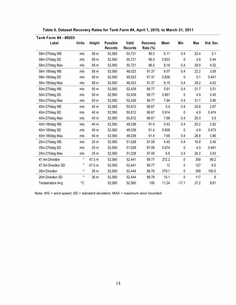
Table 6. Dataset Recovery Rates for Tank Farm #4, April 1, 2010, to March 31, 2011

Note: WS = wind speed; SD = standard deviation; MAX = maximum wind recorded

Tank Farm #4 - #9203Label Units Height Possible

RecordsValid

RecordsRecovery Rate (%)

Mean Min Max Std. Dev

58m 270deg WS m/s 58 m 52,560 50,721 96.5 6.11 0.4 22.4 3.1

58m 270deg SD m/s 58 m 52,560 50,721 96.5 0.833 0 4.9 0.44

58m 270deg Max m/s 58 m 52,560 50,721 96.5 8.18 0.4 29.9 4.02

58m 180deg WS m/s 58 m 52,560 48,023 91.37 6.07 0.4 22.2 3.08

58m 180deg SD m/s 58 m 52,560 48,023 91.37 0.838 0 5.1 0.441

58m 180deg Max m/s 58 m 52,560 48,023 91.37 8.15 0.4 29.2 4.02

50m 270deg WS m/s 50 m 52,560 52,439 99.77 5.81 0.4 21.7 3.01

50m 270deg SD m/s 50 m 52,560 52,439 99.77 0.861 0 4.9 0.45

50m 270deg Max m/s 50 m 52,560 52,439 99.77 7.94 0.4 31.1 3.96

40m 270deg WS m/s 40 m 52,560 50,812 96.67 5.4 0.4 20.6 2.87

40m 270deg SD m/s 40 m 52,560 50,812 96.67 0.914 0 4.9 0.474

40m 270deg Max m/s 40 m 52,560 50,812 96.67 7.66 0.4 29.3 3.9

40m 180deg WS m/s 40 m 52,560 48,038 91.4 5.43 0.4 20.2 2.82

40m 180deg SD m/s 40 m 52,560 48,038 91.4 0.908 0 4.9 0.473

40m 180deg Max m/s 40 m 52,560 48,038 91.4 7.68 0.4 28.8 3.86

25m 270deg WS m/s 25 m 52,560 51,028 97.09 4.45 0.4 16.9 2.45

25m 270deg SD m/s 25 m 52,560 51,028 97.09 0.974 0 4.3 0.491

25m 270deg Max m/s 25 m 52,560 51,028 97.09 6.9 0.4 26.2 3.63

47.4m Direction ° 47.5 m 52,560 52,441 99.77 272.2 0 359 99.2

47.5m Direction SD ° 47.5 m 52,560 52,441 99.77 13 0 127 6.5

26m Direction ° 26 m 52,560 52,444 99.78 279.1 0 359 100.5

26m Direction SD ° 26 m 52,560 52,444 99.78 10.1 0 117 6

Temperature Avg °C 52,560 52,560 100 11.24 -17.1 37.2 9.81

15

7.1 Data Analysis The wind data from Coddington Point and Tank Farm #4 validated by DNV was used for all of the met tower analyses. For the purposes of comparing the wind resources at Coddington Point and Tank Farm #4, the analysis in this section will examine a 12-month period where the met towers have concurrent data, April 1, 2010, to March 31, 2011.

Wind speed data were collected at 58, 50, 40, and 24 m (190, 164, 131, and 79 ft) with redundant wind speed sensors at 58 and 40 m (196 and 131 ft). The wind speed sensors were mounted on boom arms facing south (180°–190°) or west (270°–275°) to minimize met tower shading effects.

Two anemometers at Coddington Point, 58m 188 deg wind speed and 40 m 188 deg wind speed, were significantly affected by met tower shading and these data points have been flagged and removed from the datasets.

The analyses that follow group, average and sort the data utilizing a variety of methods to help illustrate important trends and other statistical data relevant to the characterization of the wind resource.

16

8 Wind Resource Assessment Summary

8.1 Wind Resource Characterization Uneven heating of the earth’s surface creates wind energy. Variation in heating and factors such as surface orientation or slope (azimuth), absorptivity (albedo), and atmospheric transmissivity also affect the wind resource. In addition, the wind resource can be accelerated, decelerated, or made turbulent by factors such as terrain, bodies of water, buildings, and vegetative cover.

Wind is air with kinetic energy that can be converted into usable energy by means of a wind turbine. Wind is a distributed resource that can generate electricity cost effectively and competitively in many regions.

8.2 Measuring Power in the Wind Wind speeds vary by season, time of day, and according to weather events.

The wind speed determines the amount of power it contains. The power available is given by:

P = ½ * A * ρ * V3

where

P = power of the wind [W]

A = windswept area of the rotor (blades) [m2] = πD2/4 = πr2

ρ = density of the air [kg/m3] (at sea level at 15°C)

V = velocity of the wind [m/s]

As shown, wind power is proportional to velocity cubed (V3). This is important to understand because as wind velocity is doubled, the available power is increased by a factor of eight (23 = 8). Consequently, what may appear to be a small increase in average speed yields a significant increase in available energy. Typically, developers looking to capture energy from higher velocity winds select taller wind turbine towers. Accordingly, the wind industry has been steadily moving toward taller towers, and the industry norm has increased from 30 m to 100 m over the last 15–20 years.

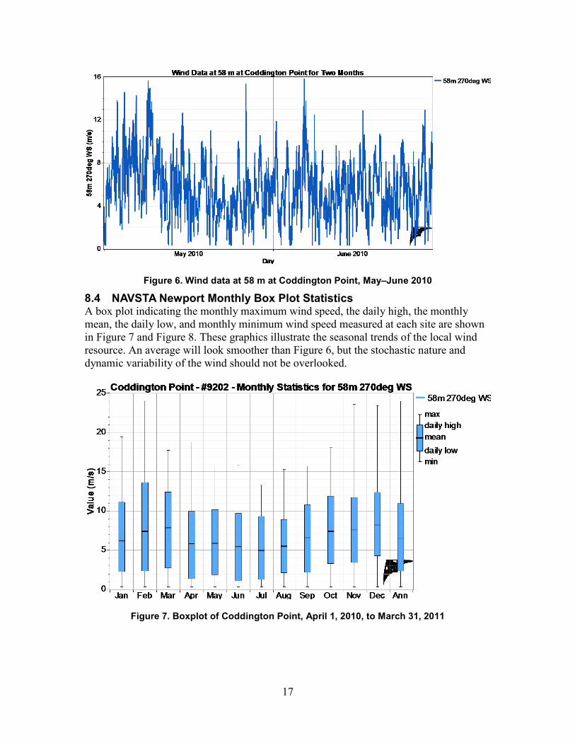
8.3 NAVSTA Newport Wind Speed Variability The wind varies widely throughout the day and night and by season as illustrated in the graph of two months of data collected at 58 m at Coddington Point in Figure 6. As shown, there are a number of 10-minute periods that have wind speeds less than 1 m/s (~2 mph). Likewise, there are many periods that have wind speeds in excess of 10 m/s (~22 mph). This sort of variability is typical, but further statistical analysis will illuminate important trends and patterns.

17

Figure 6. Wind data at 58 m at Coddington Point, May–June 2010

8.4 NAVSTA Newport Monthly Box Plot Statistics A box plot indicating the monthly maximum wind speed, the daily high, the monthly mean, the daily low, and monthly minimum wind speed measured at each site are shown in Figure 7 and Figure 8. These graphics illustrate the seasonal trends of the local wind resource. An average will look smoother than Figure 6, but the stochastic nature and dynamic variability of the wind should not be overlooked.

Figure 7. Boxplot of Coddington Point, April 1, 2010, to March 31, 2011

18

Figure 8. Boxplot of Tank Farm #4, April 1, 2010, to March 31, 2011

8.5 NAVSTA Newport Seasonal Wind Profile Figure 9 shows the wind speeds at each anemometer height as they are plotted against time to depict the seasonal trends. As can be seen in the Coddington Point graph, the fall and winter seasons were the windiest periods. Wind speeds typically increase with increased height above the ground. The collected data follows that pattern. The variation in wind speed from 24 to 58 m (79 to 190 ft) is relatively small, generally less than 1 m/s (2.2 mph). This is an indication of low VWSF. The anemometers at 180° at both 40 m and 58 m showed significant effects of tower shading and were not included in the subsequent analyses.

Figure 9. Seasonal wind speed profile at Coddington Point, April 1, 2010, to March 31, 2011

19

The data from Tank Farm #4 shows the same general seasonal trends as Coddington Point, as shown in Figure 10, though the wind speeds are generally lower at the 58 m level. Of importance is how much lower the wind speeds are at 24 m at Tank Farm #4 than at Coddington Point and the much higher resultant vertical wind shear factor (VWSF). The wind speed at 24 m at Tank Farm #4 was much lower due to the impact of the undulating terrain and trees near the met tower. At Coddington Point, most of the wind is coming off the water, so there is little to impede the flow of the wind.

Figure 10. Seasonal wind speed profile at Tank Farm #4, April 1, 2010, to March 31, 2011

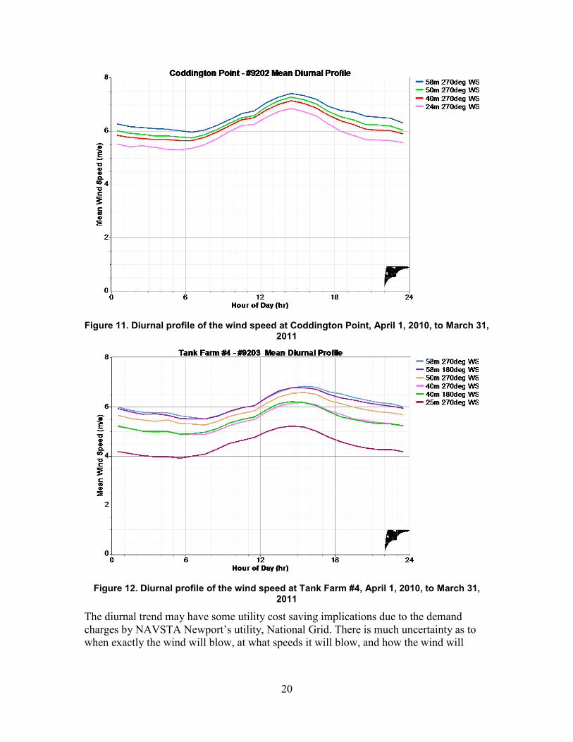
8.6 NAVSTA Newport Diurnal Wind Profile Figure 11 and Figure 12 illustrate how the wind speed varies during the course of the day. As shown, the wind speeds increase during late morning and continue increasing until mid-afternoon. Nighttime is generally the period of lower winds.

20

Figure 11. Diurnal profile of the wind speed at Coddington Point, April 1, 2010, to March 31, 2011

Figure 12. Diurnal profile of the wind speed at Tank Farm #4, April 1, 2010, to March 31, 2011

The diurnal trend may have some utility cost saving implications due to the demand charges by NAVSTA Newport’s utility, National Grid. There is much uncertainty as to when exactly the wind will blow, at what speeds it will blow, and how the wind will

21

correspond to periods of maximum loads for NAVSTA Newport. There is potential for some demand charge savings on a monthly basis, though the amount will vary widely.

Figures 13 and 14 show the diurnal trends for each month of the year. As seen at Coddington Point, April through September has wind typically peaking in mid-afternoon. There is a similar trend at Tank Farm #4, but the variation is very pronounced at 25–60 m.

Figure 13. Monthly diurnal profile of the wind speed at Coddington Point, April 1, 2010, to March 31, 2011

22

Figure 2. Monthly diurnal profile of the wind speed at Tank Farm #4, April 1, 2010, to March 31, 2011

8.7 NAVSTA Newport Wind Direction Data Wind direction informs decisions about turbine siting to maximize exposure to the best winds and minimize exposure to turbulent winds. In this analysis of direction, the compass was divided into 16 sectors, each 22.5° in size.

8.7.1 NAVSTA Newport Wind Frequency Figure 15 shows the frequency the wind blows from each direction for Coddington Point and Tank Farm #4. At Coddington Point, the wind was “calm” or blowing at less than 3 m/s (7.67 mph) 15% of the time, compared to Tank Farm #4 where it was calm 18% of the time.

At Coddington Point, the wind blows most frequently (24% of the time) in the south through southwest arc (169°–214°). Second-most frequent (22%) is the northwest arc (281°–326°). At Tank Farm #4, the wind blows most frequently (26%) in the south through southwest arc (169°–214°). Second-most frequent (22%) is the northwest arc (281°–326°).

23

Figure 35. Wind frequency rose at Coddington Point and Tank Farm #4 at 58 m, April 1, 2010, to March 31, 2011

8.7.2 NAVSTA Newport Total Wind Energy The two total wind energy roses in Figure 16 summarize the direction the most energetic winds come from. The most energetic winds are those from the west through north arc flowing across the bay. The bay has very low surface roughness as water is smooth compared to land surfaces. At Coddington Point, though the wind most frequently comes from the south-southwest arc, the strongest winds with the most energy are from the northwest arc. The winds from the northwest (259°–326°) account for 43% of the wind energy, while those from the southwest (146°–214°) account for 23% of the wind energy. At Tank Farm #4, comparing the same sectors, the northwest provides 46% of the wind energy compared to 20% for the south-southwest sector.

In siting wind turbines at NAVSTA Newport, attention should be paid to ensuring a clear fetch to the northwest and southwest of each wind turbine to the greatest degree possible as these winds will be the most energetic. Surface obstructions (trees or buildings) in these directions should be avoided as they will increase the turbulence intensity the turbines will experience.

24

Figure 16. Total wind energy rose at Coddington Point and Tank Farm #4 at 58 m, April 1,

2010, to March 31, 2011

The monthly wind total wind energy rose at Coddington Point in Figure 17 point to both the northwest-through-north arc as strong in the winter (December through February) as a source of wind energy and the southwest sector being of prime importance during the summer (June through August). Overall, this data points to the advantage of finding sites with good fetch across the water in the northwest and southwest directions.

Figure 17. Total wind energy rose at Coddington Point by month at 58 m, April 1, 2010, to March 31, 2011

25

The same seasonal directional patterns can be seen, in Figure 18, at Tank Farm #4 as at Coddington Point with the northwest-through-north arc being strong in winter (December through February) as a source of wind energy and the southwest sector being of prime importance during the summer (June through August).

Figure 48. Total wind energy rose at Tank Farm #4 by month at 58 m, April 1, 2010, to March 31, 2011

8.8 NAVSTA Newport Wind Frequency (Probability) Distribution Figure 19 illustrates a Weibull distribution of the frequency (percent of time) that the wind at 58 m is at a given speed. There are two commonly used factors to describe the distribution function, the Weibull c and Weibull k factors. The Weibull c is the scale factor for the distribution related to the annual mean wind speed. The Weibull k value is a unitless measure indicating the shape of the distribution of the wind speeds about the mean with values ranging from 1.0–3.0.

In Figure 19, the best fit Weibull distribution parameters for the measured data at Coddington Point are k = 2.07 and c = 7.39 m/s. The distribution shows that the most frequent winds, or mode of the dataset, are between 5–7 m/s as measured by the wind sensor at 58 m.

Figure 20 shows the same distribution for Tank Farm #4. The best fit Weibull distribution parameters for the measured data are k = 2.06 and c = 6.89 m/s.

26

Figure 19. Wind frequency distribution for Coddington Point at 58 m, April 1, 2010, to March 31, 2011

Figure 20. Wind frequency distribution for Tank Farm #4 at 58 m, April 1, 2010, to March 31, 2011

0 5 10 15 20 250

2

4

6

8

10

12

14

Freq

uenc

y (%

)

Probability Distribution Function - Coddington Point

58m 270deg WS (m/s)Actual data Best-fit Weibull distribution (k=2.07, c=7.39 m/s)

0 5 10 15 20 250

2

4

6

8

10

12

14

Freq

uenc

y (%

)

Probability Distribution Function - Tank Farm #4

58m 270deg WS (m/s)Actual data Best-fit Weibull distribution (k=2.06, c=6.89 m/s)

27

8.9 Vertical Wind Shear VWSF is the change in wind speed with increasing height above ground. Typically, wind speeds increase with height. This variation of wind speed with elevation is called the vertical profile of the wind speed, or VWSF. In wind turbine engineering, the determination of VWSF is an important design parameter since: (1) it directly determines the productivity of a wind turbine on a tower of certain height, and (2) it can represent the level of cyclic mechanical loading on the wind turbine system.

Analysts typically use one of two mathematical relations to characterize the measured wind shear profile:

• Power Law profile

• Logarithmic Law profile.

8.9.1 Power Law The Power Law equation is:

V = wind speed at height of interest (e.g., hub height)

Vref = wind speed measured at height Zref

Z = height of interest (e.g., hub height)

Zref = height of measured data

α = wind shear exponent

The wind shear exponent, α, or VWSF, defines how the wind speed changes with height. When the actual wind shear value is not known, a typical value used for estimation is 0.14 (aka 1/7 Power Law). When wind speed data are available at multiple heights, the wind shear factor can be calculated using the Power Law equation.

The VWSFs from several heights with known wind speeds are used to estimate both the VWSF and wind speed at other heights of interest (e.g., turbine hub height). Depending on the type of terrain and surface roughness features, the VWSF may vary from 0.0 to 0.4.

Z u

Z ref

V = V ref

28

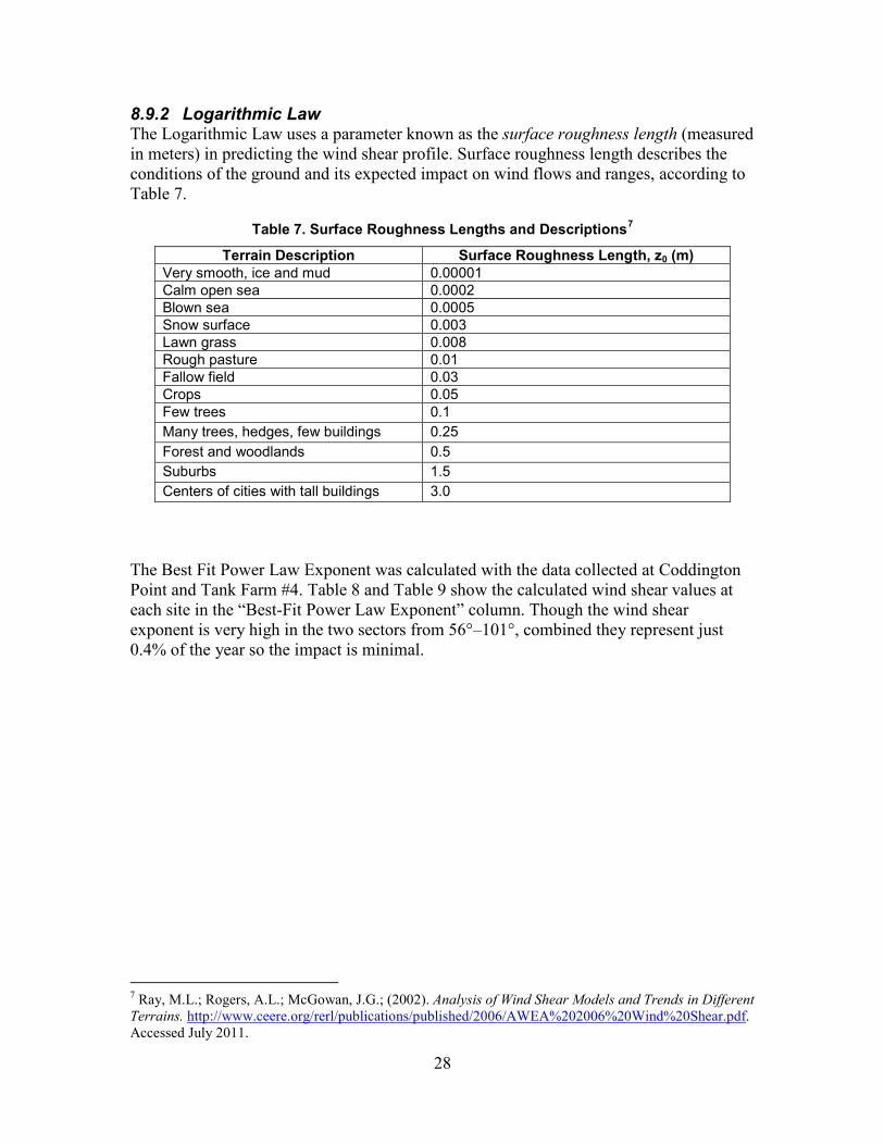
8.9.2 Logarithmic Law The Logarithmic Law uses a parameter known as the surface roughness length (measured in meters) in predicting the wind shear profile. Surface roughness length describes the conditions of the ground and its expected impact on wind flows and ranges, according to Table 7.

Table 7. Surface Roughness Lengths and Descriptions7

Terrain Description Surface Roughness Length, z0 (m) Very smooth, ice and mud 0.00001 Calm open sea 0.0002 Blown sea 0.0005 Snow surface 0.003 Lawn grass 0.008 Rough pasture 0.01 Fallow field 0.03 Crops 0.05 Few trees 0.1 Many trees, hedges, few buildings 0.25 Forest and woodlands 0.5 Suburbs 1.5 Centers of cities with tall buildings 3.0

The Best Fit Power Law Exponent was calculated with the data collected at Coddington Point and Tank Farm #4. Table 8 and Table 9 show the calculated wind shear values at each site in the “Best-Fit Power Law Exponent” column. Though the wind shear exponent is very high in the two sectors from 56°–101°, combined they represent just 0.4% of the year so the impact is minimal.

7 Ray, M.L.; Rogers, A.L.; McGowan, J.G.; (2002). Analysis of Wind Shear Models and Trends in Different Terrains. http://www.ceere.org/rerl/publications/published/2006/AWEA%202006%20Wind%20Shear.pdf. Accessed July 2011.

29

Also shown in Table 8 is the application of surface roughness lengths. The surface roughness parameter is “solved for” from the existing wind speed data at various heights. The resultant characterization may not always match the actual surface conditions, but it serves as a descriptor of the vertical wind shear profile. The surface roughness lengths have been calculated for Coddington Point and Tank Farm #4 and are shown in “Surface Roughness” column at the far right in Table 8 and Table 9. As shown, there is a marked difference in the surface roughness characteristics between the two sites. Most of the wind coming into the met tower at Coddington point is over water, grass, parking lots, or roads. There are some taller buildings to the east that are the cause of the high surface roughness lengths shown in the two sectors from 56°–101°. These sectors represent wind data from 0.4% of the year so the overall impact is minimal.

Table 8. Power Law Exponent and Surface Roughness Length for Coddington Point, April 1, 2010, to March 31, 2011

58m 270° WS

50m 270° WS

40m 270° WS

24m 270° WS

° # m/s m/s m/s m/s unitless m

348.75° - 11.25° 3,926 6.507 6.405 6.340 6.091 0.073 0.00003811.25° - 33.75° 2,533 6.786 6.534 6.322 5.506 0.235 0.50405533.75° - 56.25° 1,048 5.631 5.362 5.184 4.534 0.24 0.55495256.25° - 78.75° 136 3.117 2.850 2.692 2.105 0.433 3.56061478.75° - 101.25° 36 1.284 0.928 0.877 0.829 0.392 3.525177101.25° - 123.75° 324 4.938 4.637 4.413 3.926 0.25 0.676891123.75° - 146.25° 1,742 5.876 5.644 5.443 5.055 0.164 0.085183146.25° - 168.75° 2,428 6.181 5.908 5.750 5.417 0.14 0.029994168.75° - 191.25° 4,581 5.598 5.333 5.151 4.880 0.145 0.039881191.25° - 213.75° 7,234 6.738 6.533 6.292 5.887 0.15 0.047117213.75° - 236.25° 3,473 6.143 5.889 5.709 5.342 0.151 0.049494236.25° - 258.75° 2,339 5.739 5.465 5.322 4.979 0.15 0.049262258.75° - 281.25° 2,983 6.356 6.103 5.999 5.693 0.115 0.006509281.25° - 303.75° 5,066 7.474 7.241 7.148 6.885 0.085 0.000316303.75° - 326.25° 5,651 7.550 7.321 7.269 7.028 0.073 0.000044326.25° - 348.75° 4,213 7.121 6.977 6.933 6.707 0.063 0.000005Overall Annual Figure 6.605 6.383 6.245 5.904 0.121 0.009460

Direction Sector Time Steps

Mean Wind Speed Best-Fit Power Law

Exponent

Surface Roughness

30

The surface roughness lengths at Tank Farm #4, as seen in Table 9 below, are much higher in all directions due to the hills, trees, and vegetation nearby.

Table 9. Power Law Exponent and Surface Roughness Length for Tank Farm #4, April 1, 2010, to March 31, 2011

58m 270° WS

58m 180° WS

50m 270° WS

40m 270° WS

40m 180° WS

24m 270° WS

° # m/s m/s m/s m/s m/s m/s unitless m

348.75° - 11.25° 80 4.611 4.119 4.422 4.019 3.589 3.354 0.343 2.02465911.25° - 33.75° 2,643 5.663 5.542 5.386 4.863 4.816 3.949 0.426 3.49782833.75° - 56.25° 1,721 5.067 5.056 4.770 4.322 4.351 3.520 0.434 3.66549356.25° - 78.75° 730 4.093 4.121 3.807 3.384 3.445 2.616 0.537 5.67435878.75° - 101.25° 0101.25° - 123.75° 958 5.521 5.525 5.215 4.655 4.763 3.779 0.455 4.070293123.75° - 146.25° 1,663 5.523 5.452 5.240 4.699 4.729 3.770 0.455 4.049013146.25° - 168.75° 2,778 5.819 5.699 5.493 4.932 4.918 3.708 0.534 5.542946168.75° - 191.25° 4,114 5.198 5.130 4.952 4.507 4.482 3.533 0.461 4.128535191.25° - 213.75° 8,538 6.175 6.159 5.951 5.525 5.518 4.621 0.349 2.076652213.75° - 236.25° 3,038 5.410 5.453 5.147 4.663 4.749 3.866 0.406 3.140462236.25° - 258.75° 2,157 5.226 5.262 4.933 4.413 4.531 3.435 0.507 5.043667258.75° - 281.25° 2,944 6.241 6.272 5.957 5.483 5.559 4.412 0.419 3.322762281.25° - 303.75° 5,573 7.547 7.556 7.335 6.940 6.993 5.702 0.34 1.884309303.75° - 326.25° 5,346 7.246 7.224 7.096 6.739 6.744 5.752 0.28 1.010974326.25° - 348.75° 3,687 6.792 6.713 6.641 6.219 6.197 5.274 0.305 1.352402Overall Annual Figure 6.172 6.144 5.935 5.487 5.506 4.502 0.379 2.590000

Direction Sector Time Steps

Mean Wind Speed Best-Fit Power Law

Exponent

Surface Rough-

ness

31

Figure 21 shows graphs comparing the measured data to the Power Law approach to vertical wind shear versus the Logarithmic Law approach. Both methods track closely with the measured data and each other at Coddington Point. There is a wider spread between these methods at lower and higher wind speeds at Tank Farm #4. The Power Law was used for energy calculations as it is tied more closely to statistical calculations rather than surface roughness approximations.

As shown, at a height of 100 m above the ground, the impact of surface roughness is negated and the wind speeds are all assumed to be 10 m/s. With low surface roughness (designated by z0 = 0.00001 m), the wind speed decreases minimally, moving closer to the ground such that even as low as 5 m above the ground, the wind speed is 8 m/s; that is, it has only decreased 20% despite a 95% reduction in height above the ground. With high surface roughness associated with cities and high buildings (designated by z0 = 3 m), the wind speed decreases by 20% with only a 50% reduction in height above the ground, and the wind speed is reduced by 50% at approximately 18 m above the ground or a reduction in height of 82%. These phenomena impact the energy production estimates for Coddington Point and Tank Farm #4.

Figure 21. Vertical wind shear profile at Coddington Point and Tank Farm #4 at 58 m, April 1, 2010, to March 31, 2011

32

The daily wind shear at Coddington Point as it varies by month is shown in Figure 22. The months with the higher wind shears generally have lower wind speeds, especially during nighttime hours.

Figure 22. Daily wind shear profile by month at Coddington Point, April 1, 2010, to March 31, 2011

At Tank Farm #4, the patterns are similar, though the overall values are much higher.

Figure 23. Daily wind shear profile by month at Tank Farm #4, April 1, 2010, to March 31, 2011

33

8.10 Turbulence Intensity Turbulence intensity (TI) is the standard deviation of the wind speed within a time step divided by the mean wind speed over that same time step. TI is a measure of the gustiness of the wind. High turbulence is associated with increased wind turbine system wear and increased operation and maintenance (O&M) costs. At lower wind speeds, the calculated turbulence intensity is higher, as seen in Figure 24. However, the higher turbulence at low wind speeds is not a concern because of the low power available at those low wind speeds. Turbulence at higher winds speeds is of greater interest and concern to wind turbine manufacturers.

Turbulence analysis determines the suitable types of turbine designs for a wind energy project. Because wind turbines must withstand a variety of wind conditions, design standards have been developed by the International Electrotechnical Commission (IEC). The IEC 61400-1:20058 has two components—one for wind speed and one for turbulence—and can be seen in Table 10. The standard designates four different classes of wind turbines, I through IV, which are designed for varying degrees of wind resource, with Class I being very high mean wind speed and Class IV being low mean wind speed.

The standard also designates a wind turbulence classification, A through C, that describes the amount of turbulence a turbine must be designed to withstand, with A being the highest turbulence and C being the lowest. In recent years, wind turbine manufacturers have introduced designs for sites with lower wind speeds and low turbulence known as low wind speed turbines. These turbines have larger rotors, for a given generator size, and are thus capable of producing significantly more annual energy at a low wind speed site than the Class I or II or Class A or B turbines of similar generator size.

There are several types of TI of interest. The representative TI, for a set of 10-minute time steps, is equal to the 90th percentile of the TI values. Assuming a normal distribution of these values, it represents the mean value plus 1.28 standard deviations. The mean TI is the mean value of all of the TI data at a particular wind speed.

Table 10 displays design wind speed and mean turbulence intensity ratings for the different wind turbine design classes.

8 International Electrotechnical Commission (IEC). “International Standard IEC 61400-1 Third Edition.” Geneva, Switzerland: IEC, 2005.

34

Table 10. IEC Wind Turbine Classes, Ratings, and Characteristics of Turbulence Intensity9

Figure 24 shows the representative and mean TI as a function of wind speed at 58 m at Coddington Point.

Figure 24. Representative and mean turbulence intensities for Coddington Point, April 1, 2010, to March 31, 2011

9 IEC/TC88, 61400-1 ed. 3, Wind turbines - Part 1: Design Requirements, International Electrotechnical Commission (IEC), 2005.

WTG* Class IEC I High Wind

IEC II Medium

Wind

IEC III Low Wind

IEC IV Low Wind

Vav e average wind speed at hub-height (m/s) 10 8.5 7.5 6

V50 extreme 50-year gust (m/s) 70 59.5 52.5 42

Mean turbulence intensity at 15 m/s - turbulence Class A

Mean turbulenceiIntensity at 15 m/s - turbulence Class B

Mean turbulence intensity at 15 m/s - turbulence Class C* Wind Turbine Generator

14% - 16%

12% - 14%

0 - 12%

35

Figure 25 shows the IEC turbulence ratings relative to the representative TI. A point of primary interest is the mean TI at 15 m/s, which is 0.101 (10.1%). This indicates low turbulence and that a Class C wind turbine is possible.

Figure 25. Turbulence intensity for Coddington Point at 58 m, April 1, 2010, to March 31, 2011

The same traits are graphed in Figure 26 for Tank Farm #4. The difference in the turbulence between these two sites can be seen readily in the Representative TI (blue line) in each graph. The impact of the turbulence findings is that a Class B wind turbine is most suitable for Tank Farm #4, which will result in lower annual energy production from a given manufacturer’s turbines (Class B versus Class C).

Quantity ValueRecords in 15 m/s bin 421Mean T I at 15 m/s 0.101Representative T I at 15 m/s 0.135IEC3 turbulence category C

36

Figure 26. Turbulence intensity for Tank Farm #4 at 58 m, April 1, 2010, to March 31, 2011

Additional visual displays of the turbulence data and analyses can be seen in Appendix B.

8.11 Energy Production Potential of Coddington Point and Tank Farm #4 Using a full year of concurrent wind data collected at both Coddington Point and Tank Farm #4, along with the turbulence factors determined by analysis and the turbine height restrictions based on Federal Aviation Administration (FAA) permits, a comparative analysis of the energy production potential at these two sites was conducted to determine the viability of each site.

The maximum permitted height for each site is shown in Table 11. Based on the turbulence analysis in the previous section, a representative Class C wind turbine (low turbulence) was identified as appropriate for Coddington Point, and a similar Class B turbine was identified as appropriate for Tank Farm #4. A low wind speed turbine on an 80 m (263 ft) tower is in compliance with the FAA-permitted height at Coddington Point. A rotor designed for mid-range wind speeds and turbulence installed on a 64.7 m (212 ft) tower is in compliance with the FAA-permitted height at Tank Farm #4.

Quantity ValueRecords in 15 m/s bin 263Mean T I at 15 m/s 0.122Representative T I at 15 m/s 0.165IEC3 turbulence category B

37

Table 11. FAA-Permitted Heights and Turbine Dimensions

Table 12 and Table 13 show the results of the turbine energy outputs. An overall loss factor of 13.4% at each site was included in these calculations. The turbine at Coddington Point has been modeled to produce 748,000 kWh more per year than at Tank Farm #4, resulting in approximately $82,000 cost savings per year, or over $1.6 million over the 20-year expected life of the turbines. Given this differential, the energy production analysis for the base will focus on those sites with minimal FAA height restrictions.

Table 12. Coddington Point Energy Production with Low Wind Speed Class C Turbine

Potential Turbine Site

Turbine Model

FAA Height Limit

Hub Height

Blade Length

Total Height

FAA Height Limit

Hub Height

Blade Length

Total Height

# m m m m ft ft ft ftCoddington Point GE 1.5 xle 139.9 80.0 41.3 121.3 459 262.5 135.3 397.8Tank Farm # 4 A GE 1.5 sle 103.3 64.7 38.5 103.2 339 212.3 126.3 338.6Tank Farm # 4 B GE 1.5 sle 88.4 61.4 38.5 99.9 290 201.4 126.3 327.8

Coddington Point GE 1.5 xle 80 m tower

Hub Height Wind Speed

Time at Zero Output

Time at Rated Output

Mean Net Power Output

Mean Net Energy Output

Net Capacity Factor

Month (m/s) (%) (%) (kW) (kWh/yr) (%)Jan 6.38 11.1 6.3 419.0 311,716 27.9Feb 7.58 5.9 14.7 536.5 360,557 35.8Mar 7.90 3.4 14.7 592.4 440,718 39.5Apr 6.08 6.9 2.3 347.8 250,448 23.2May 6.16 5.3 3.0 354.8 263,970 23.7Jun 5.67 6.0 0.7 280.1 201,674 18.7Jul 5.18 9.5 0.3 225.8 167,992 15.1Aug 5.86 7.3 3.5 307.6 228,832 20.5Sep 6.85 4.8 3.5 451.6 325,128 30.1Oct 7.66 4.2 8.9 567.8 422,457 37.9Nov 7.82 4.2 14.0 582.2 419,158 38.8Dec 8.38 4.8 17.7 602.2 448,010 40.1

Overall 6.79 6.1 7.5 438.9 3,844,637 29.3

38

Table 13. Tank Farm #4 Energy Production with Medium Wind Speed Class B Turbine

Tank Farm #4 GE 1.5 s le 64.7m tower

Hub Height Wind Speed

Time at Zero Output

Time at Rated Output

Mean Net Power Output

Mean Net Energy Output

Net Capacity Factor

Month (m/s) (%) (%) (kW) (kWh/yr) (%)Jan 6.31 17.0 4.8 373.2 277,671 24.9Feb 7.45 8.7 11.8 471.8 317,069 31.5Mar 7.42 7.9 7.4 498.2 370,635 33.2Apr 5.68 17.5 2.0 260.5 187,532 17.4May 5.72 17.1 2.2 254.9 189,628 17.0Jun 5.20 18.7 0.1 181.8 130,864 12.1Jul 4.82 21.8 0.0 145.7 108,432 9.7Aug 5.22 20.5 0.1 196.0 145,828 13.1Sep 6.22 13.8 0.4 317.9 228,895 21.2Oct 7.27 9.4 5.3 467.7 347,957 31.2Nov 7.22 10.4 3.8 477.4 343,731 31.8Dec 8.22 8.3 10.5 603.8 449,223 40.3Overall 6.39 14.3 4.0 353.4 3,095,995 23.6

39

9 MiniSODAR Data

The miniSODAR was first deployed at Coddington Point at the South Pritchard Field site in February 2009 and was then moved to other locations at NAVSTA Newport, as shown in Table 4 in Section 6.4. The objective was to provide wind speed data throughout the span of the rotor to effectively compare the wind resource at potential turbine sites with varying surface roughness features. Analysis to date of the wind speed data from the miniSODAR does not correlate well with the data collected from the met towers, increasing the uncertainty of using the miniSODAR data for energy production estimates across the base.

40

10 Long-Term Data Adjustment

It is important to determine if the data monitoring period is representative of the long-term wind resource at the site. Different methodologies are used to estimate the long-term wind resource at the site where the short-term met tower study was conducted. A standard industry approach with a number of variations is measure-correlate-predict (MCP), where a short-term dataset is correlated to a long-term wind dataset from a nearby monitoring station (reference site). The correlation relationship is then applied to the measured data at the site of interest to project the expected long-term wind resource. An industry-standard MCP method, the ratio of the mean of monthly means, was used in this analysis.

The purpose of this estimate is to provide a normalized, realistic estimate of the long-term wind resource and the resultant wind turbine energy production. Though wind turbine production at any site will vary year-to-year, the goal is to have the long-term energy production estimate minimize the uncertainty of the relatively short period of collected data.

10.1 Long-Term Datasets The Federal Aviation Administration (FAA) and National Weather Service (NWS) own and operate automated surface observing systems (ASOS) for the purposes of aviation and weather observation. These datasets generally represent the most consistent weather observation data as the FAA and NWS are tasked with building an historical long-term surface weather observation record. Other long-term weather observation datasets include military airfield observations, ocean buoy observations, and other forms of surface observations.

10.1.1 Wind Speed Sensor Change Over the past decade, the NWS has replaced cup-type anemometers at ASOS stations with sonic anemometers to improve data capture rates, data recovery, and measurement reliability. These two wind speed measurement sensors, however, do not uniformly record the same wind speeds. Industry analysis of this issue has resulted in widespread acceptance of using a correction factor of 3% to increase the wind speed readings of the sonic anemometers relative to either cup or propeller anemometers.10

Four long-term reference stations are within an 8.5-mile radius of the Coddington Point met tower. The monthly data recovery rates for these stations were examined for site suitability. Two of the sites did not have records that overlapped the met tower observation period and thus were automatically excluded. Site #725074, Quonset State Airport in Rhode Island, had an average data recovery rate of 39.3% over the met tower observation period, which is insufficient to provide adequate confidence in long-term wind adjustments. Thus, Site #725079, Newport State Airport, was used for the MCP analysis. Figure 27 shows the data recovery rates from 1998 to 2011.

10 ams.confex.com/ams/pdfpapers/69268.pdf. Accessed August 2011.

41

Figure 27. Monthly data recovery rates at Newport Airport, December 1998–March 2011

10.1.2 Newport Airport Data Newport Airport (ASOS) is approximately 2.5 miles from the Coddington Point met tower location and had a monthly average data recovery rate over 98% for the period of 1998 to 2011. The anemometer is mounted at 10 m above ground level (AGL). Several months had significant periods of missing data due to instrumentation changes or other issues. Data from months where data recovery rates were below 85% were not used in the MCP process. However, those monthly averages were replaced with the average of all of the same months from all other available years with sufficient data recovery rates so as not to skew the yearly averages.

As mentioned earlier, ASOS stations have undergone a fleet-wide upgrade to sonic anemometers in recent years. At Newport Airport, the change in anemometry occurred on September 26, 2006.11 Data collected on or after that date have been adjusted upward by 3% according to standard industry practice. The revised long-term annual mean wind speeds can be seen in Figure 28.

11 Lewis, R.; Dover, J.; Field and Operational Tests of a Sonic Anemometer for the Automated Surface Observing System. http://www.nws.noaa.gov/asos/pdfs/IFW_stat.pdf. Accessed August 2011.

0102030405060708090

100

Dec-98 Aug-01 May-04 Feb-07 Nov-09Perc

ent o

f Dat

a R

ecov

ered

Time

Monthly Data Recovery Rates at Newport Airport #725079

Monthly Data Recovery Rates at Airport #725079

42

Figure 28. Corrected long-term annual mean wind speeds and overall mean annual wind speed at Newport Airport, January 1, 1999, to March 31, 2011

Note: 2011 includes data through March 31, 2011

In the graph in Figure 29, the collected data from Coddington Point is displayed relative to the collected data during the same timeframe at Newport Airport. Also shown is the long-term monthly means at Newport Airport during each of the months the Coddington Point met tower was collecting data. Visually, the sites represent similar winds based on the similarity in their patterns over time, though it should be noted that the Newport Airport met tower is at 10 m versus 25, 40, and 60 m at Coddington Point; thus, the magnitude of the winds are much lower at Newport Airport than at Coddington Point.

Figure 29. Collected data at Coddington Point versus collected and long-term data at

Newport Airport

3.3

3.4

3.5

3.6

3.7

3.8

3.9

4

4.1

4.2

1999 2001 2003 2005 2007 2009 2011

Win

d Sp

eed

(m/s

)

Time (yr)

Annual Mean Wind Speed at Newport State Airport - #725079

Corrected Long Term Annual Mean Wind Speeds

Mean Annual Wind Speed 1999-2010

2.0

2.5

3.0

3.5

4.0

4.5

5.0

5.5

6.0

6.5

7.0

7.5

8.0

8.5

9.0

Jun-09 Sep-09 Jan-10 Apr-10 Jul-10 Oct-10 Feb-11

Win

d Sp

eed

(m/s

)

Monthly Mean Wind Speed Comparison Bewteen Coddington Point and Newport Airport July 2009-March 2011

58 m 270° at Coddington Point

40 m 270° at Coddington Point

25 m at Coddington Point

10 m at Newport Airport

Long Term Mean Monthly Wind Speed at Newport Airport

43

10.1.3 Measure-Correlate-Predict With the long-term data at Newport Airport adjusted for the wind sensor change out, the data was examined to determine if the period of collection (at Coddington Point and Newport Airport) represents a normal, higher-than-normal, or lower-than-normal wind year. The MCP method employed to analyze the data used the ratio of the mean of monthly means approach. This method involves using the ratio of the monthly means of the long-term data to the monthly means during the period of collection to determine a monthly adjustment factor to be applied to the measured data at Coddington Point, so it will represent long-term data trends and characteristics.

In Table 14, the “Ratio of Monthly Means” column is the ratio of the long-term monthly means at Newport Airport to the monthly means during the data collection period at Newport Airport. That ratio is multiplied by the monthly means during the data collection period from Coddington Point at 40 m and 58 m. The results in the two columns at the far right represent the expected long-term mean monthly wind speed at 40 m and 58 m at Coddington Point. These adjusted wind speeds are used in the wind flow modeling and energy production estimates in Section 11.

Table 14. Newport Airport and Coddington Point Data Adjusted to Long-Term Trends

Figure 30 illustrates graphically the adjustment to the Coddington Point data through the MCP analysis. With this adjustment, the data is now representative of the local long-term wind trends.

Station

Height WS @ 10 m WS @ 10 m WS @ 40 m WS @ 58 m WS @ 40 m WS @ 58 m

Period 7/09 - 3/11 1/99 - 3/11 7/09 - 3/11 7/09 - 3/11 Long-Term Mean Long-Term MeanUnit m/s m/s m/s m/s m/s m/sJul-09 2.89 2.93 1.02 5.42 5.96 5.51 6.05Aug-09 2.56 2.68 1.05 4.75 5.05 4.98 5.30Sep-09 2.76 3.16 1.14 5.08 5.42 5.81 6.19Oct-09 3.92 3.66 0.93 6.86 7.26 6.41 6.78Nov-09 3.90 3.99 1.02 6.48 6.86 6.62 7.01Dec-09 4.89 4.32 0.88 7.76 8.02 6.87 7.10Jan-10 4.34 4.24 0.98 6.96 7.24 6.81 7.08Feb-10 4.57 4.29 0.94 6.67 7.05 6.27 6.62Mar-10 4.64 4.43 0.95 6.94 7.45 6.62 7.10Apr-10 3.21 4.12 1.28 5.44 5.85 6.98 7.49May-10 3.14 3.67 1.17 5.57 5.92 6.51 6.92Jun-10 2.85 3.16 1.11 5.06 5.43 5.62 6.03Jul-10 2.67 2.93 1.10 4.63 4.97 5.09 5.46Aug-10 3.02 2.68 0.89 5.09 5.55 4.52 4.92Sep-10 3.36 3.16 0.94 6.17 6.62 5.80 6.22Oct-10 3.82 3.66 0.96 7.04 7.45 6.75 7.15Nov-10 4.15 3.99 0.96 7.33 7.64 7.04 7.35Dec-10 4.86 4.32 0.89 7.93 8.21 7.05 7.30Jan-11 3.70 4.24 1.15 6.06 6.28 6.96 7.21Feb-11 4.03 4.29 1.06 7.08 7.42 7.54 7.90Mar-11 4.59 4.43 0.96 7.24 7.94 6.97 7.65

Coddington Point Coddington Point Adjusted WSNewport Airport Ratio of Monthly Means

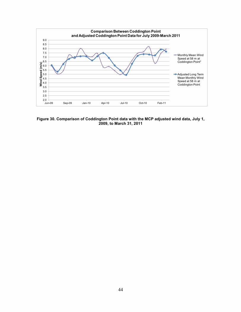
44

Figure 30. Comparison of Coddington Point data with the MCP adjusted wind data, July 1, 2009, to March 31, 2011

2.02.53.03.54.04.55.05.56.06.57.07.58.08.59.0

Jun-09 Sep-09 Jan-10 Apr-10 Jul-10 Oct-10 Feb-11

Win

d Sp

eed

(m/s

)

Comparison Between Coddington Point and Adjusted Coddington Point Data for July 2009-March 2011

Monthly Mean Wind Speed at 58 m at Coddington Point"

Adjusted Long Term Mean Monthly Wind Speed at 58 m at Coddington Point

45

11 Energy Production Estimates

This section discusses the potential energy generation from wind turbines at NAVSTA Newport. Several layout scenarios and turbine types were evaluated using a common wind flow model and wake model approach. The approximately 9 MW project scenarios result in a spread of approximately 24–30 GWh/yr of energy production and capacity factors of 30%–36%. A full economic analysis is recommended, but this is generally considered a moderate to good production potential when held in the context of local energy costs.

Analysis was conducted for a larger build out by assuming the siting of utility-scale turbines at every viable site. The results of these analyses can be found in Appendix D.

11.1 Wind Turbines Modeled A broad range of utility-scale wind turbine models were selected to represent potential project scenarios at NAVSTA Newport. These turbines were selected based upon IEC turbine type as well as general availability and access to the power curves. These turbines generally represent low wind and moderate wind classifications. The range of turbines is generally intended to showcase the available turbines with large nameplate capacities (1.6 MW or greater) as well as the new generation of low wind machines, which couple an enlarged rotor with a standard generator. All power curves were for sea level air density at 1.225 kg/m3. The turbine models are shown in Table 15.

Table 15. Wind Turbine Specifications Used in Modeling

11.2 Site Layout Overall, 16 available sites were evaluated for turbine installation given the available FAA determination of no hazard (DNH) filings. Many sites were eliminated from this review because their DNH height restriction was well below the level of all utility-scale turbines under review for this project. NREL recommends working with the FAA and local air space managers to further investigate the viability of height restriction easing should NAVSTA Newport feel the remaining available sites are insufficient. Table 16 includes a list of all FAA DNH sites along with their respective total heights.

Turbine Manufacturer, Size, and Model

Nameplate Capacity

Turbine Class

Hub Height

Rotor Span

Max Height

Max Height

9 MW Scenario

MW # m m m ft # turbinesSiemens 2.3 MW 101 2.3 III 80 101 130.5 428 4GE 1.6 XLE-100 1.6 III 80 100 130 427 6RePower MM100 1.8 III 80 100 130 427 5

Vestas V100 1.8 MW 1.8 III 80 100 130 427 5Alstom ECO 110 3.0 MW 3 IIa 75 110 130 427 3Nordex N100 2.5 III 80 100 130 427 4Vestas V112 3.0 MW 3 III 84 112 140 459 3

46

Table 16. FAA-Approved Heights at Each Site

Table 17 shows the viable FAA sites based upon turbine maximum tip height. These figures assumed the standard tower for each turbine—typically 80 m (262 ft). The selected turbines represent a reasonable sampling of IEC Class II and III wind turbines with IEC Turbulence Class C rating. Overall, there are seven sites that can accommodate these turbines. The turbine selection here by no means represents an endorsement of a particular wind turbine over another suitability-rated turbine. There are a number of other factors to consider in the turbine selection process, including cost, availability, constructability, transportability, warranty, the types of other proximal wind turbines, and O&M.

Site Name

Deg Min Sec Zone Deg Min Sec Zone FAA - AGL*

FAA - AMSL**

Site Elevation -

ASL***

Max Turbine Height

° ' " dir ° ' " dir m m m mCoddington Point Bishop Rock 41 31 3.56 N 71 19 49.86 W 139.9 143.0 3.0 139.9Building 6/ Derecktor Shipyard 41 31 29.47 N 71 18 41.00 W 102.1 106.7 4.6 102.1Coddington Point Bldg 1112 41 31 22.73 N 71 19 24.95 W 139.9 152.1 12.2 139.9Bldg 1285 CP 41 31 11.38 N 71 18 58.14 W 105.2 106.7 1.5 105.2Katy Field 41 30 50.00 N 71 19 40.47 W 139.9 144.5 4.6 139.9NUWC 41 32 12.55 N 71 18 26.74 W 89.6 106.7 17.1 89.6Pritchard Field North 41 31 9.17 N 71 19 38.30 W 139.9 144.5 4.6 139.9Pritchard Field South 41 31 3.04 N 71 19 37.11 W 139.9 143.0 3.0 139.9Coastal Harbor Island Helipad 41 30 14.28 N 71 19 33.91 W 139.9 144.5 4.6 139.9Tank Farm 3 41 34 11.98 N 71 17 16.06 W 88.4 115.5 27.1 88.4Tank Farm 3 A 41 34 16.60 N 71 17 18.38 W 93.6 115.5 21.9 93.6Tank Farm 4 A 41 33 53.14 N 71 17 40.62 W 103.3 115.5 12.2 103.3Tank Farm 4 B 41 33 53.60 N 71 17 25.48 W 88.4 115.5 27.1 88.4Tank Farm 5 41 33 8.05 N 71 18 17.24 W 90.2 103.3 13.1 90.2Tank Farm 5 C 41 32 52.79 N 71 18 12.49 W 64.3 93.0 28.7 64.3W36 CP 41 30 42.04 N 71 19 20.66 W 139.9 146.0 6.1 139.9*FAA AGL is the FAA Above Ground limit

**FAA AMSL is the FAA Above Mean Sea Level limit

***Above Sea Level

Lat (NAD 83) Long(NAD 83)

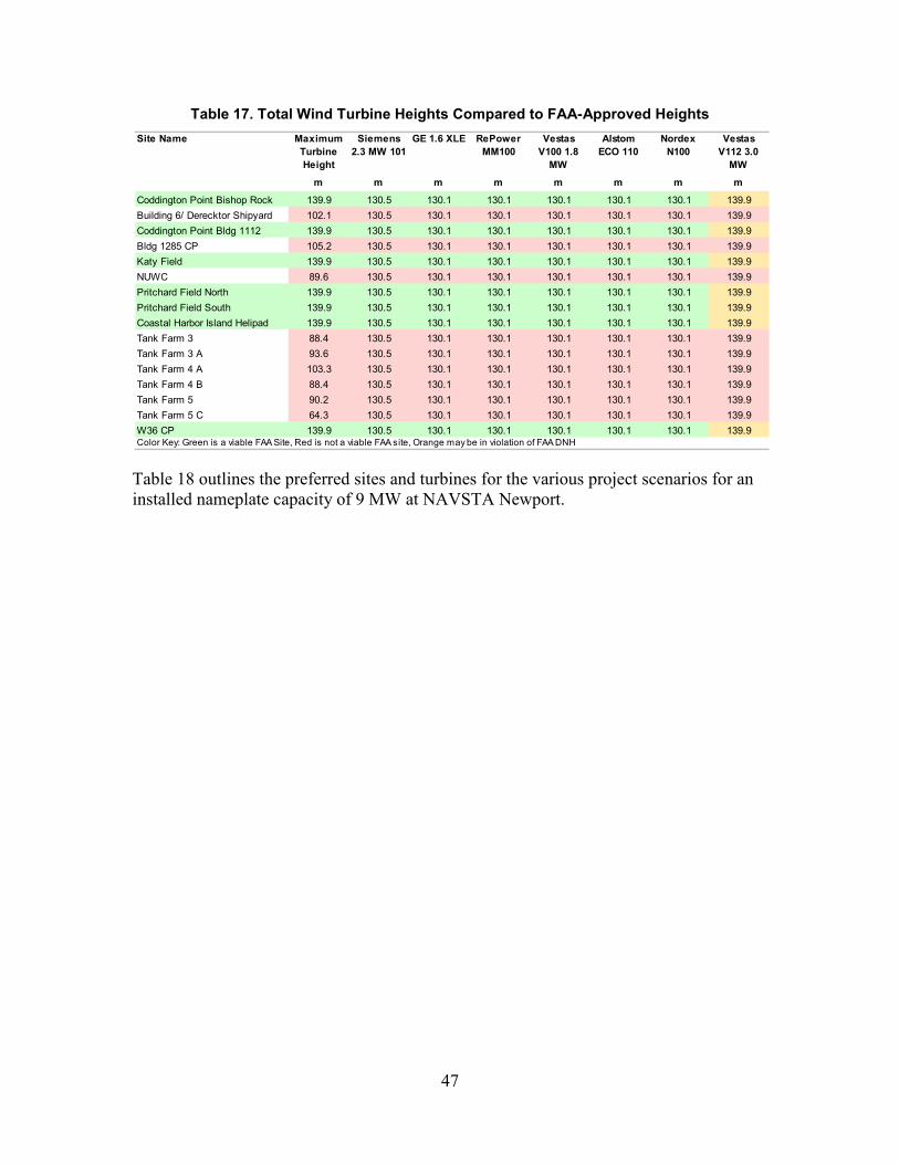
47

Table 17. Total Wind Turbine Heights Compared to FAA-Approved Heights

Table 18 outlines the preferred sites and turbines for the various project scenarios for an installed nameplate capacity of 9 MW at NAVSTA Newport.

Site Name Maximum Turbine Height

Siemens 2.3 MW 101

GE 1.6 XLE RePower MM100

Vestas V100 1.8

MW

Alstom ECO 110

Nordex N100

Vestas V112 3.0

MW

m m m m m m m m

Coddington Point Bishop Rock 139.9 130.5 130.1 130.1 130.1 130.1 130.1 139.9Building 6/ Derecktor Shipyard 102.1 130.5 130.1 130.1 130.1 130.1 130.1 139.9Coddington Point Bldg 1112 139.9 130.5 130.1 130.1 130.1 130.1 130.1 139.9Bldg 1285 CP 105.2 130.5 130.1 130.1 130.1 130.1 130.1 139.9Katy Field 139.9 130.5 130.1 130.1 130.1 130.1 130.1 139.9NUWC 89.6 130.5 130.1 130.1 130.1 130.1 130.1 139.9Pritchard Field North 139.9 130.5 130.1 130.1 130.1 130.1 130.1 139.9Pritchard Field South 139.9 130.5 130.1 130.1 130.1 130.1 130.1 139.9Coastal Harbor Island Helipad 139.9 130.5 130.1 130.1 130.1 130.1 130.1 139.9Tank Farm 3 88.4 130.5 130.1 130.1 130.1 130.1 130.1 139.9Tank Farm 3 A 93.6 130.5 130.1 130.1 130.1 130.1 130.1 139.9Tank Farm 4 A 103.3 130.5 130.1 130.1 130.1 130.1 130.1 139.9Tank Farm 4 B 88.4 130.5 130.1 130.1 130.1 130.1 130.1 139.9Tank Farm 5 90.2 130.5 130.1 130.1 130.1 130.1 130.1 139.9Tank Farm 5 C 64.3 130.5 130.1 130.1 130.1 130.1 130.1 139.9W36 CP 139.9 130.5 130.1 130.1 130.1 130.1 130.1 139.9Color Key: Green is a viable FAA Site, Red is not a viable FAA site, Orange may be in violation of FAA DNH

48

Table 18. Recommended Turbine Per Project Size Parameter of 9 MW

11.3 Energy Production Loss Factors All energy projects will incur some type of energy loss due to real-world conditions differing from the idealized case. The resulting decrease in efficiency is often accounted for by a series of estimated and calculated loss factors. The loss factors for the NAVTSA project include:

• Array efficiency: This loss parameter is associated with the wakes created by the turbines. This results in a decrease in wind speed and increase in turbulence as the wind moves through the wind farm array. This is a value calculated by the OpenWind12 wind farm design model.

12 OpenWind, AWSTruepower, http://www.awsopenwind.org/. Accessed August 4, 2011.

Preferred 3 Turbine SetupIndex Site Easting [m] Northing [m] Applicable Turbine Models Total Project Size

1 Coddington Point Bishop Rock 305533.93 4598846.67 Vestas V112 3.0MW 9 MW2 Coddington Point Bldg 1112 306127.02 4599422.36 Alstom ECO 110 9 MW3 Katy Field 305740.56 4598422.58

Preferred 4 Turbine SetupIndex Site Easting [m] Northing [m] Applicable Turbine Models Total Project Size

1 Coddington Point Bishop Rock 305533.93 4598846.672 Coddington Point Bldg 1112 306127.02 4599422.36 Nordex N100 2.5 MW 10 MW3 Pritchard Field North 305807.48 4599012.45 Siemens 2.3 MW 9.2 MW4 Katy Field 305740.56 4598422.58

Preferred 5 Turbine SetupIndex Site Easting [m] Northing [m] Applicable Turbine Models Total Project Size

1 Coddington Point Bishop Rock 305533.93 4598846.672 Coddington Point Bldg 1112 306127.02 4599422.36 Vestas V100 1.8 MW 9 MW3 Pritchard Field North 305807.48 4599012.45 RePower MM100 1.8MW 9 MW4 Katy Field 305740.56 4598422.585 Building 6/ Derecktor Shipyard 307152.42 4599602.88

Preferred 6 Turbine SetupIndex Site Easting [m] Northing [m] Applicable Turbine Models Total Project Size

1 Coddington Point Bishop Rock 305533.93 4598846.672 Coddington Point Bldg 1112 306127.02 4599422.363 Pritchard Field North 305807.48 4599012.45 GE 1.6 XLE-100 9.6 MW4 Katy Field 305740.56 4598422.585 Building 6/ Derektor Shipyard 307152.42 4599602.886 Building 1283/ Navy Lodge 306740.20 4599055.59

7 Turbine Setup (All)Index Site Easting [m] Northing [m] Applicable Turbine Models Total Project Size

1 Coddington Point Bishop Rock 305533.93 4598846.672 Coddington Point Bldg 1112 306127.02 4599422.363 Pritchard Field North 305807.48 4599012.454 Katy Field 305740.56 4598422.58 All Turbines 9-10 MW5 Building 6/ Derektor Shipyard 307152.42 4599602.886 Building 1283/ Navy Lodge 306740.20 4599055.597 Pritchard Field South 305830.20 4598822.64

Note: Green shading represents viable turbine(s) at the selected sites

49

• Topographic efficiency: This parameter relates to the increase or decrease in wind resource across the project due to topographic influences. This can be a positive or negative value and is dependent on the location of the meteorological measurements along with the model used to predict flow across the site. See Section 11.4 for further discussion of the modeling approach used.

• Turbine availability: This term accounts for the expected downtime a wind turbine will experience during its annual operation. This includes routine maintenance, faults, and any component failures. Turbine availability or uptime is typically covered in the manufacturer’s warranty terms with a value of 95% or greater.

• Electrical: Electrical losses occur in the process of collecting and transmitting the project energy across the site. As the power moves through the transformers and collection system, a certain percentage will be lost as heat. This value is typically estimated at 2%.

• Hysteresis: This is the term for when a turbine shuts down to protect itself from ambient climate events that are outside of the design envelope. This typically involves a high wind event that forces the turbine to shut down for a predetermined amount of time. The NAVSTA site did not show any evidence of regular high wind events and therefore is not expected to incur losses from hysteresis.

• Environmental: Environmental losses occur because of ambient conditions that may affect blade aerodynamics or turbine operation. This includes icing, blade soiling, insect accumulation, and extreme cold or hot events. This is expected to happen at NAVSTA and is anticipated to be on the order of 1%.

• Operational: All operational energy requirements such as power for the control system, heating system, and other parasitic loads.

• Power curve variation: The power curve may deviate from the manufacturer-stated designation due to yaw system misalignment, incorrect programming, or ambient weather events such as high turbulence or variations in atmospheric stability. This was not believed to be an issue for NAVSTA.

• Sector management: Sector management can be required if the wind rose has multiple directions that affect the turbine layout.

• Substation downtime: The collection substation on the NAVSTA Newport side of the utility interconnection will likely require some downtime for routine maintenance. This is estimated at 0.5% for NAVSTA.

• Utility downtime: Utility transmission and distribution uptime or availability is generally very high. However, there are certain areas of the country or seasons of the year with more risk. The NAVSTA site is assumed to experience energy loss of 0.5% due to the utility electrical system being unavailable for power transmission.

50

Table 19 lists the range of efficiencies used to determine wind turbine energy production. The bottom row provides an estimate of the net productive efficiency of each turbine in the 9 MW scenarios.

Table 19. Site Production Annual Loss Factors for the 9 MW Scenario

11.4 Site Climatology NREL evaluated the available sites by creating a wind flow model of the project area. This project area is composed of the viable turbine sites per Section 11.2. The wind flow model was created using the Wind Atlas Analysis and Application Program13 (WAsP) from Risø Technical University of Denmark. WAsP is a linearized formulation of the Reynolds Averaged Navier Stokes (RANS) equations. WAsP can account for moderate changes in terrain and surface roughness when used in conjunction with measured met data. WAsP provides a map of wind speed up and slow down relative to the measurement location known as a wind resource grid. In this way, estimates of the general performance of potential turbine sites across the project area are derived. This analysis employed terrain information from the National Elevation Dataset14 (NED), along with aerial imagery from the National Agriculture Imagery Program15 (NAIP). The WAsP model was run with a horizontal grid resolution of 25 m and an elevation of 80 m above ground level. Figure 31 shows the 80 m hub height mean wind speed map for all direction sectors.

13 WAsP – Wind Atlas Analysis and Application Program. Software – WasP Version 10.01.0100. http://www.wasp.dk/index_old.htm. Accessed August 2, 2011. 14 National Elevation Dataset, U.S. Geological Survey. http://ned.usgs.gov/. Accessed August 2, 2011. 15 National Agriculture Imagery Program, Farm Service Agency, U.S. Department of Agriculture, http://www.fsa.usda.gov/FSA/apfoapp?area=home&subject=prog&topic=nai. Accessed August 2, 2011.

Characteristic Unit Siemens 2.3 MW 101

GE 1.6 XLE RePower MM100

Vestas V100 1.8 MW

Alstom ECO 110

Nordex N100

Vestas V112 3.0 MW

Maximum Blade Tip Height ft 428 427 427 427 427 427 459*Array Efficiency % 94.47 95.25 95.67 96.94 94.59 95.82 96.91*Topographic Efficiency % 97.90 96.76 97.27 97.23 97.88 97.25 97.12Turbine Availability % 95.00 95.00 95.00 95.00 95.00 95.00 95.00Plant Electrical Efficiency % 98.00 98.00 98.00 98.00 98.00 98.00 98.00Hysteresis % 100.00 100.00 100.00 100.00 100.00 100.00 100.00Environmental % 99.00 99.00 99.00 99.00 99.00 99.00 99.00Operational % 100.00 100.00 100.00 100.00 100.00 100.00 100.00Power Curve Variation % 100.00 100.00 100.00 100.00 100.00 100.00 100.00Sector Management % 100.00 100.00 100.00 100.00 100.00 100.00 100.00Substation Maintenance % 99.50 99.50 99.50 99.50 99.50 99.50 99.50Utility Downtime % 99.00 99.00 99.00 99.00 99.00 99.00 99.00Total Losses % 16.02 16.33 15.51 14.42 15.93 15.39 14.55Net Production % 83.98 83.67 84.49 85.58 84.07 84.61 85.45*Calculated Loss factor

Turbine Manufacturer /Model

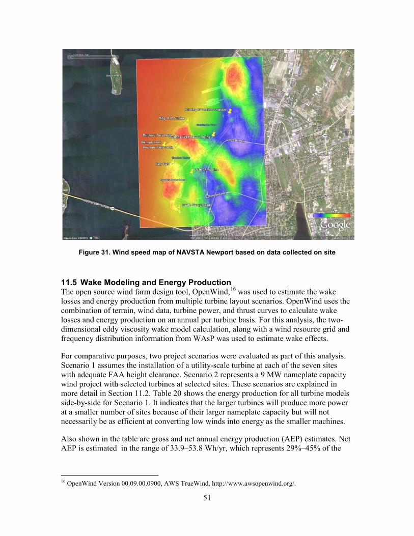
51

Figure 31. Wind speed map of NAVSTA Newport based on data collected on site

11.5 Wake Modeling and Energy Production The open source wind farm design tool, OpenWind,16 was used to estimate the wake losses and energy production from multiple turbine layout scenarios. OpenWind uses the combination of terrain, wind data, turbine power, and thrust curves to calculate wake losses and energy production on an annual per turbine basis. For this analysis, the two-dimensional eddy viscosity wake model calculation, along with a wind resource grid and frequency distribution information from WAsP was used to estimate wake effects.

For comparative purposes, two project scenarios were evaluated as part of this analysis. Scenario 1 assumes the installation of a utility-scale turbine at each of the seven sites with adequate FAA height clearance. Scenario 2 represents a 9 MW nameplate capacity wind project with selected turbines at selected sites. These scenarios are explained in more detail in Section 11.2. Table 20 shows the energy production for all turbine models side-by-side for Scenario 1. It indicates that the larger turbines will produce more power at a smaller number of sites because of their larger nameplate capacity but will not necessarily be as efficient at converting low winds into energy as the smaller machines.

Also shown in the table are gross and net annual energy production (AEP) estimates. Net AEP is estimated in the range of 33.9–53.8 Wh/yr, which represents 29%–45% of the

16 OpenWind Version 00.09.00.0900, AWS TrueWind, http://www.awsopenwind.org/.

52

annual electricity consumption at NAVSTA Newport (approximately 105 GWh/yr).17 The net capacity factors range from 27.2%–34.8%.

Table 20. Annual Energy Production Figures for One Wind Turbine at Each of the Seven Sites at NAVSTA Newport

Table 21 shows the energy production for all turbine models side-by-side for Scenario 2. It shows the estimated AEP figures of the project scenarios targeting approximately 9 MW of wind capacity. This table highlights the potential real-world scenarios and the resulting energy production.

Net AEP is estimated to be in the 23.7–30.0 GWh/yr range, which represents 22%–29% of the annual electricity consumption at NAVSTA Newport (approximately 105 GWh/yr).18 The net capacity factors range from 30.0%–36.4%.

Table 21. Annual Energy Production Figures for Approximately 9 MW of Wind at NAVSTA Newport

17 FY 2009 data from Reichert, J. Email. NAVSTA Newport, Newport, RI, 14 February 2011. 18 FY 2009 data from Reichert, J. Email. NAVSTA Newport, Newport, RI, 14 February 2011.

Characteristics Unit 7 Turbines - All Sites ScenarioWTG* Manufacturer Siemens GE Vestas Vestas Nordex REPower AlstomWTG Model # 2.3 MW XLE 100 V100 V112 N100 MM100 ECO 110WTG Capacity MW 2.3 1.6 1.8 3.0 2.5 1.8 3.0WTG Hub Height m 80 80 80 80 80 80 80WTG Rotor Diameter m 101 100 100 112 100 100 110Array Size # 7 7 7 7 7 7 7Site Capacity MW 16.10 11.20 12.60 21.00 17.50 12.60 21.00Ideal Yield GWh/yr 54.73 43.55 48.58 70.43 56.14 49.16 65.78Gross AEP Central Estimate GWh/yr 52.29 41.73 46.59 67.32 53.60 47.14 62.76Net AEP Central Estimate GWh/yr 42.02 33.91 37.83 53.79 43.15 38.39 50.07Net Capacity Factor % 29.79 34.56 34.28 29.24 28.15 34.78 27.22*WTG = Wind Turbine Generator; AEP = Annual Energy Production

Characteristics Unit ~9 MW ScenarioWTG* Manufacturer Siemens GE Vestas Vestas Nordex REPower AlstomWTG Model # 2.3 MW XLE 100 V100 V112 N100 MM100 ECO 110WTG Capacity MW 2.3 1.6 1.8 3.0 2.5 1.8 3.0WTG Hub Height m 80 80 80 80 80 80 80WTG Rotor Diameter m 101 100 100 112 100 100 110Array Size # 4 6 5 3 4 5 3Site Capacity MW 9.20 9.60 9.00 9.00 10.00 9.00 9.00Ideal Yield GWh/yr 31.27 37.33 34.70 30.19 32.08 35.11 28.19Gross AEP Central Estimate GWh/yr 30.79 35.65 33.50 29.56 31.57 33.89 27.59Net AEP Central Estimate GWh/yr 25.74 30.05 28.35 25.36 26.44 28.73 23.67Net Capacity Factor % 31.93 35.73 35.95 32.17 30.18 36.44 30.02*WTG = Wind Turbine Generator; AEP = Annual Energy Production

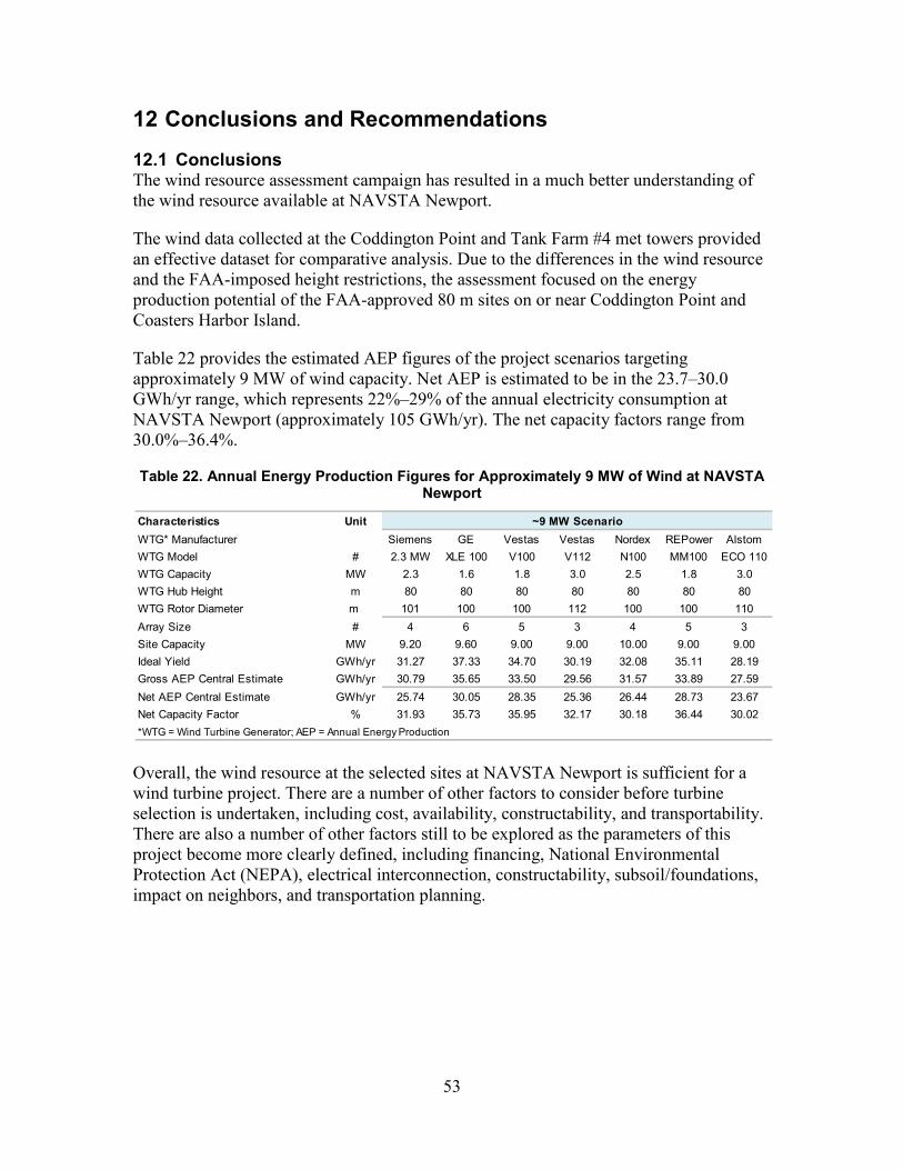
53

12 Conclusions and Recommendations

12.1 Conclusions The wind resource assessment campaign has resulted in a much better understanding of the wind resource available at NAVSTA Newport.

The wind data collected at the Coddington Point and Tank Farm #4 met towers provided an effective dataset for comparative analysis. Due to the differences in the wind resource and the FAA-imposed height restrictions, the assessment focused on the energy production potential of the FAA-approved 80 m sites on or near Coddington Point and Coasters Harbor Island.

Table 22 provides the estimated AEP figures of the project scenarios targeting approximately 9 MW of wind capacity. Net AEP is estimated to be in the 23.7–30.0 GWh/yr range, which represents 22%–29% of the annual electricity consumption at NAVSTA Newport (approximately 105 GWh/yr). The net capacity factors range from 30.0%–36.4%.

Table 22. Annual Energy Production Figures for Approximately 9 MW of Wind at NAVSTA Newport

Overall, the wind resource at the selected sites at NAVSTA Newport is sufficient for a wind turbine project. There are a number of other factors to consider before turbine selection is undertaken, including cost, availability, constructability, and transportability. There are also a number of other factors still to be explored as the parameters of this project become more clearly defined, including financing, National Environmental Protection Act (NEPA), electrical interconnection, constructability, subsoil/foundations, impact on neighbors, and transportation planning.

Characteristics UnitWTG* Manufacturer Siemens GE Vestas Vestas Nordex REPower AlstomWTG Model # 2.3 MW XLE 100 V100 V112 N100 MM100 ECO 110WTG Capacity MW 2.3 1.6 1.8 3.0 2.5 1.8 3.0WTG Hub Height m 80 80 80 80 80 80 80WTG Rotor Diameter m 101 100 100 112 100 100 110Array Size # 4 6 5 3 4 5 3Site Capacity MW 9.20 9.60 9.00 9.00 10.00 9.00 9.00Ideal Yield GWh/yr 31.27 37.33 34.70 30.19 32.08 35.11 28.19Gross AEP Central Estimate GWh/yr 30.79 35.65 33.50 29.56 31.57 33.89 27.59Net AEP Central Estimate GWh/yr 25.74 30.05 28.35 25.36 26.44 28.73 23.67Net Capacity Factor % 31.93 35.73 35.95 32.17 30.18 36.44 30.02*WTG = Wind Turbine Generator; AEP = Annual Energy Production

~9 MW Scenario

54

12.2 Recommendations There are a number of tasks ahead to continue to move this project forward, including:

• NAVSTA Newport to complete the NEPA evaluation already underway

• NREL/DNV to complete an electrical interconnection study

• Complete the economic feasibility study

• Complete the transportation and logistics study

55

Appendix A. Met Tower Sensors

Met tower components for NAVSTA Newport at Coddington Point and Tank Farm #4:

• NRG Systems 60 m XHD Tower: o Six NRG Systems #40C anemometers (item 1899)

o Two NRG Systems #200P wind vanes (item 1904)

o One NRG Systems #110S temperature sensor (item 1906)

o One SymphoniePLUS® data logger (item 4289)

• NRG Systems #40C Anemometer (item: 1899). The NRG Systems #40C Maximum anemometer is the industry standard anemometer used worldwide. NRG Systems #40C anemometers have recorded wind speeds of 96 m/s (214 mph). Their low moment of inertia and unique bearings permit very rapid response to gusts and lulls. Because of their output linearity, these sensors are ideal for use with various data retrieval systems. A four-pole magnet induces a sine wave voltage into a coil producing an output signal with a frequency proportional to wind speed. The #40C is constructed of rugged Lexan cups molded in one piece for repeatable performance. A rubber terminal boot is included.

Figure A-1. Anemometer #40C NRG Systems (item 1899)19

• NRG Systems #200P Wind Direction Vane, 10K (item: 1904). The NRG Systems #200P wind direction vane is the industry standard wind direction vane used worldwide. The thermoplastic and stainless steel components resist corrosion and contribute to a high strength-to-weight ratio. The vane is directly connected to a precision conductive plastic potentiometer located in the main body. An analog voltage output directly proportional to the wind

19 Photo courtesy of NRG Systems, Inc. http://www.nrgsystems.com/AllProducts/SensorsandTurbineControl.aspx

56

direction is produced when a constant DC excitation voltage is applied to the potentiometer. A rubber terminal boot is included.

Figure A-2. Wind vane NRG Systems #200P (item 1904)20

• Mounting booms. NRG side-mounting booms allow you to easily mount sensors to your tower or mast at any height. Mounting hardware is included. Heavy-duty mounting booms are designed specifically for icing environments and mounting NRG IceFree sensors.

Figure A-3. Boom, side, 1.53m (60.5"), galvanized, with clamps (item: 3390)21

20 Photo courtesy of NRG Systems, Inc. http://www.nrgsystems.com/AllProducts/SensorsandTurbineControl.aspx 21 Photo courtesy of NRG Systems, Inc. http://www.nrgsystems.com/AllProducts/SensorsandTurbineControl.aspx

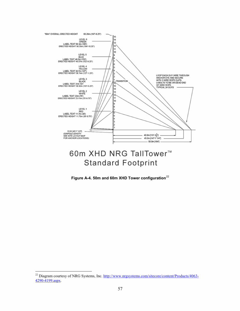
57

Figure A-4. 50m and 60m XHD Tower configuration22

22 Diagram courtesy of NRG Systems, Inc. http://www.nrgsystems.com/sitecore/content/Products/4063-4290-4199.aspx.

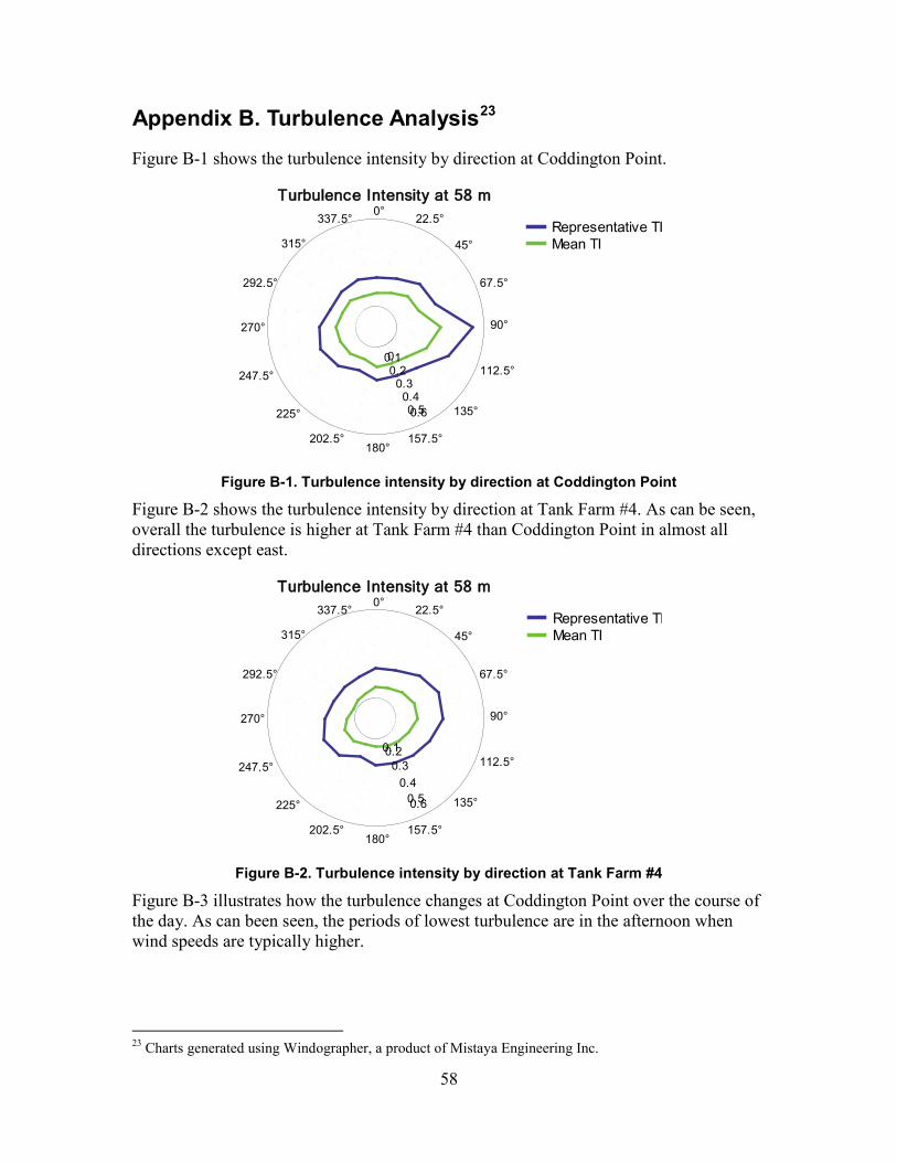
58

Appendix B. Turbulence Analysis23

Figure B-1 shows the turbulence intensity by direction at Coddington Point.

Figure B-1. Turbulence intensity by direction at Coddington Point

Figure B-2 shows the turbulence intensity by direction at Tank Farm #4. As can be seen, overall the turbulence is higher at Tank Farm #4 than Coddington Point in almost all directions except east.

Figure B-2. Turbulence intensity by direction at Tank Farm #4

Figure B-3 illustrates how the turbulence changes at Coddington Point over the course of the day. As can been seen, the periods of lowest turbulence are in the afternoon when wind speeds are typically higher.

23 Charts generated using Windographer, a product of Mistaya Engineering Inc.

Turbulence Intensity at 58 m0°

22.5°

45°

67.5°

90°

112.5°

135°

157.5°180°

202.5°

225°

247.5°

270°

292.5°

315°

337.5°

00.10.20.30.40.50.6

Representative TIMean TI

Turbulence Intensity at 58 m0°

22.5°

45°

67.5°

90°

112.5°

135°

157.5°180°

202.5°

225°

247.5°

270°

292.5°

315°

337.5°

0.10.20.3

0.40.50.6

Representative TIMean TI

59

Figure B-3. Diurnal turbulence intensity at 58 m at Coddington Point

Figure B-4. Diurnal turbulence intensity at 58 m at Tank Farm #4

60

Figure B-5. Seasonal turbulence intensity at 58 m at Coddington Point

Figure B-6. Seasonal turbulence intensity at 58 m at Tank Farm #4

61

Figure B-7 shows a plot of the turbulence intensity versus wind speed at Coddington Point. As shown, the windier it was, the less turbulence there was in the wind.

Figure B-7. Turbulence intensity vs. wind speed at Coddington Point

Figure B-8 shows a plot of the turbulence intensity versus wind speed at Tank Farm #4.

Figure B-8. Turbulence intensity vs. wind speed at Tank Farm #4

62

Appendix C. Additional Site Information

Though the report was essentially completed using metric units, one table in particular, Table 16, was considered of interest to base personnel and is included (Table C-1) with English units for reference.

Table C-1. FAA-Approved Heights for Each Site

Site Name

Deg Min Sec Zone Deg Min Sec Zone FAA - AGL*

FAA - AMSL**

Site Elevation -

ASL***

Max Turbine Height

° ' " dir ° ' " dir ft ft ft ftCoddington Point Bishop Rock 41 31 3.56 N 71 19 49.86 W 459 469 10 459Building 6/ Derecktor Shipyard 41 31 29.47 N 71 18 41.00 W 335 350 15 335Coddington Point Bldg 1112 41 31 22.73 N 71 19 24.95 W 459 499 40 459Bldg 1285 CP 41 31 11.38 N 71 18 58.14 W 345 350 5 345Katy Field 41 30 50.00 N 71 19 40.47 W 459 474 15 459NUWC 41 32 12.55 N 71 18 26.74 W 294 350 56 294Pritchard Field North 41 31 9.17 N 71 19 38.30 W 459 474 15 459Pritchard Field South 41 31 3.04 N 71 19 37.11 W 459 469 10 459Coastal Harbor Island Helipad 41 30 14.28 N 71 19 33.91 W 459 474 15 459Tank Farm 3 41 34 11.98 N 71 17 16.06 W 290 379 89 290Tank Farm 3 A 41 34 16.60 N 71 17 18.38 W 307 379 72 307Tank Farm 4 A 41 33 53.14 N 71 17 40.62 W 339 379 40 339Tank Farm 4 B 41 33 53.60 N 71 17 25.48 W 290 379 89 290Tank Farm 5 41 33 8.05 N 71 18 17.24 W 296 339 43 296Tank Farm 5 C 41 32 52.79 N 71 18 12.49 W 211 305 94 211W36 CP 41 30 42.04 N 71 19 20.66 W 459 479 20 459*FAA AGL is the FAA Above Ground limit

**FAA AMSL is the FAA Above Mean Sea Level limit

***Above Sea Level

Lat (NAD 83) Long(NAD 83)