neural model of stereoacuity and depth interpolation based ... model of stereoacuity and... ·...

The Journal of Neuroscience, July 1990, 70(7): 2281-2299

Neural Model of Stereoacuity and Depth Interpolation Based on a Distributed Representation of Stereo Disparity

Sidney R. Lehky and Terrence J. Sejnowski”

Department of Biophysics, Johns Hopkins University, Baltimore, Maryland 21218

We have developed a model for the representation of stereo disparity by a population of neurons that is based on tuning curves similar in shape to those measured physiologically (Poggio and Fischer, 1977). Signal detection analysis was applied to the model to generate predictions of depth discrimination thresholds. Agreement between the model and human psychophysical data was possible in this model only when the population size representing disparity in a small patch of visual field was in the range of about 20-200 units. Interval encoding and rate encoding were found to be inconsistent with these data. Psychophysical data on stereo interpolation (Westheimer, 1988a) suggest that there are short-range excitatory and long-range inhibitory interactions between disparity-tuned units at nearby spatial locations. We extended our population model of disparity coding at a single spatial location to include such lateral interactions. When there was a small disparity gradient between stimuli at 2 locations, units in the intermediate, unstimulated position developed a pattern of activity corresponding to the average of the 2 lateral disparities. When there was a large disparity gradient, units at the intermediate position developed a pattern of activity corresponding to an independent superposition of the 2 lateral disparities, so that both disparities were represented simultaneously. This mixed population pattern may underlie the perception of depth discontinuities and transparent surfaces. Similar types of distributed representations may be applicable to other parameters, such as orientation, motion, stimulus size, and motor coordinates.

Ever since the time of Wheatstone (1838) it has been known that disparities between images presented to the 2 eyes induce a strong senstation of depth. Julesz (1960, 197 1) has shown that disparity is sufficient in itself, without monocular cues, for stereopsis. Disparity-tuned neurons in visual cortex were first dem- onstrated by Barlow et al. (1967), Nikara et al. (1968) and Pettigrew et al. (1968) in cats, and by Hubel and Wiesel(l970) in monkeys. More recently, Poggio and colleagues have recorded extensively within areas V 1 and V2 of macaque visual cortex

Received Sept. 5, 1989; revised Feb. 5, 1990; accepted Feb. 14, 1990. Supported by a grant from the Sloan Foundation to T.J.S. and G. F. Poggio.

S.R.L. was supported by the McDonnell Foundation during preparation of the manuscript. Portions of this work were reported at the 1987 and 1988 annual meetings of the Association for Research in Vision and Ophthalmology.

Correspondence should be addressed to Sidney R. Lehky, Room lN- 107, Build- ing 9, Laboratory of Nemopsychology, National Institute of Mental Health, Be- thesda, MD 20892.

a Present address: Computational Neurobiology Laboratory, The Salk Institute, P.O. Box 85800, San Diego, CA 92138.

Copyright 0 1990 Society for Neuroscience 0270-6474/90/072281-19$03.00/O

[see Poggio and Poggio (1984) for a review of these studies]. In this paper we develop a model for the representation of disparity based on both the psychophysical and physiological data. Al- though the focus is on binocular vision, the ideas presented here generalize to the neural representation of other parameters.

The psychophysical data of central interest involve measurements of the discriminability between different disparities. The primary physiological data are measurements of disparity tuning for neurons in monkey cortex. By requiring theory to be consistent with 2 different sources of constraints, the range of possible models is greatly restricted. The modeling starts with a consideration of a population of disparity-tuned units at a single location of the visual field, and the sensitivity of this population to small changes in depth, or stereoacuity. Following this, psychophysical data concerning interactions between nearby stimuli at different depths are taken into account by adding lateral connections between units at different locations. The result is not a complete model of stereopsis, but only addresses one part of the problem-the representation of disparity.

Alternative encodings of disparity

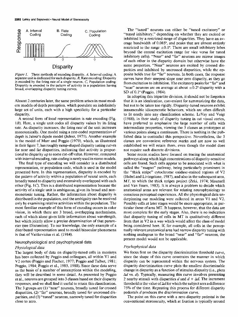
There are a number of ways to represent disparity, which can be placed into 2 broad categories, local representations or distributed representations. In a local representation, disparity is unambiguously represented by the activity of a single neuron. An example of this is shown in Figure lA, where the value of disparity is indicated by which neuron fires. For instance, the vigorous firing of a certain neuron means that the disparity is, say 5.0’, but if some other neuron fires then the disparity is 7.0’, and so forth. To cover the entire range of disparities there must be a large number of such narrowly tuned units with minimal overlap, each indicating that the stimulus disparity falls within a particular small interval. This form of local representation is called interval encoding, and has been used almost universally in models of stereopsis (Nelson, 1975; Marr and Poggio, 1976; Mayhew and Frisby, 1981; Pollard et al., 1985; Pradzny, 1985; Szeliski and Hinton, 1985, among others; see Szeliski, 1986, for a review of these models).

A problem with interval coding is the need for many units to achieve a high degree of resolution. This was pointed out long ago by Young (1802) as he argued against interval coding and for population coding in color vision:

As it is almost impossible to conceive each sensitive point of the retina to contain an infinite number of particles, each vibrating in perfect unison with every possible modulation, it becomes necessary to suppose the number limited; for instance to the three principle colours. . . .

2282 Lehky and Sejnowski * Neural Model of Stereoacuity

0 A. Interval B. Rate

E Coding Coding C. Population

Coding

B ___ ___ 12 u

I 0 0 0

Disparity Figure I. Three methods of encoding disparity. A, Interval coding: A separate unit is dedicated for each disparity. B, Rate encoding: Disparity is encoded by the firing rate of a single neuron. C, Population coding: Disparity is encoded in the pattern of activity in a population having broad, overlapping disparity tuning curves.

Almost 2 centuries later, the same problem arises in most mod- em models of depth perception, which postulate an indefinitely large set of units, each with a high specificity for a particular disparity.

A second form of local representation is rate encoding (Fig. 1B). Here, a single unit codes all disparity values by its firing rate. As disparity increases, the firing rate of the unit increases monotonically. One model using a rate-coded representation of depth is Julesz’s dipole model (Julesz, 197 1). Another example is the model of Mat-r and Poggio (1979), which, as illustrated in their figure 7, has roughly ramp-shaped disparity tuning curves for near and far disparities, indicating that activity is proportional to disparity up to some cut-off value. However, compared with interval encoding, rate-coding is rarely used in stereo models.

The final type of encoding we will consider is a distributed representation, or population code, which is used in the model presented here. In this representation, disparity is encoded by the pattern of activity within a population of neural units, each broadly tuned to disparity and extensively overlapped with each other (Fig. 1 C’). This is a distributed representation because the activity of a single unit is ambiguous, given its broad and non- monotonic tuning. Rather, the information about disparity is distributed in the population, and the ambiguity can be resolved only by examining relative activities within the population. The most familiar example of this form of encoding occurs in color vision, in which there are 3 broad, overlapping mechanisms, each of which alone gives little information about wavelength, but which jointly allow a precise determination of that parameter (see Discussion). To our knowledge, the only example of a distributed representation used to model binocular phenomena is that of Vaitkevicius et al. (1984).

Neurophysiological and psychophysical data

Physiological data The largest body of data on disparity-tuned cells in monkeys has been collected by Poggio and colleagues, all within Vl and V2 cortex (Poggio and Fischer, 1977; Poggio and Talbot, 198 1; Poggio, 1984; Poggio et al., 1985, 1988). Since these data serve as the basis of a number of assumptions within the modeling, they will be described in some detail. As presented by Poggio et al., neurons are grouped into 3 classes based on their disparity responses, and we shall find it useful to retain this classification. The 3 groups are (1) “near” neurons, broadly tuned for crossed disparities, (2) “far” neurons, broadly tuned for uncrossed disparities, and (3) “tuned” neurons, narrowly tuned for disparities close to zero.

The “tuned” neurons can either be “tuned excitatory” or “tuned inhibitory,” depending on whether they are excited or inhibited by a restricted range of disparities. They have an average bandwidth of 0.085”, and peaks that are almost entirely restricted to the range kO.1”. There are small inhibitory lobes beyond the central excitation range (or vice versa for tuned inhibitory cells). “Near” and “far” neurons are mirror images of each other in the disparity domain but otherwise have the same properties. “Near” neurons are excited by crossed disparities and inhibited by uncrossed disparities, while the opposite holds true for “far” neurons. In both cases, the response curves have their steepest slope near zero disparity, as they go from excitation to inhibition. The excitatory peaks for “far” and “near” neurons are on average at about kO.2” disparity with a SD of 0.1” (Poggio, 1984).

In adopting this tripartite division, it should not be forgotten that it is an idealization, convenient for summarizing the data, but not to be taken too rigidly. Disparity-tuned neurons exhibit innumerable idiosyncratic behaviors, which are often difficult to fit neatly into any classification scheme. LeVay and Voigt (1988), in their study of disparity tuning in cat visual cortex, have preferred to emphasize the large number of cells with intermediate properties, viewing the 3 classes as prototypes at various points along a continuum. There is nothing in the pub- lished data to contradict this perspective. Nevertheless, the 3 classes are convenient reference marks and are now so well established we will retain them, even though the model does not require such discrete divisions.

Some recent studies have focused on tracing the anatomical pathways along which high concentrations of disparity-sensitive cells are found. Such cells appear to be associated with what is called the “magno” pathway, being particularly prominent in the “thick stripe” cytochrome oxidase-stained regions of V2 (Hubel and Livingstone, 1987), and also in the subsequent area, MT, to which the thick stripes project (Zeki, 1974; Maunsell and Van Essen, 1983). It is always a problem to decide which anatomical areas are relevant for relating neurophysiology to conscious perceptual experiences. All the physiological data un- derpinning our modeling were collected in areas Vl and V2. Possibly cells at later stages would be more appropriate, in particular those of area MT. It happens, however, that the data are most complete for the early stages. Also, there is no indication that disparity tuning of cells in MT is qualitatively different from that in V2 in a way which would affect the class of model being considered here. If, for example, all cells in the perceptually relevant anatomical area had narrow disparity tuning with nothing analogous to the broad “near” and “far” neurons, the present model would not be applicable.

Psychophysical data

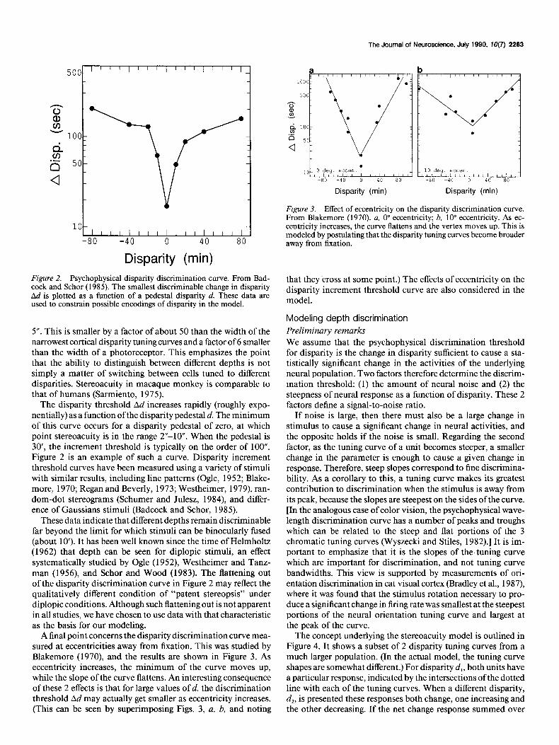
We focus first on the disparity discrimination threshold curve, since the shape of this curve constrains the manner in which disparity can be represented within the nervous system. The disparity discrimination curve plots the smallest discriminable change in disparity as a function of stimulus disparity (i.e., plots Ad vs. d). Typically, measuring this curve involves presenting 2 nearby stimuli with disparities d and d + Ad. The increment threshold is the value ofAd for which the subject sees a difference 75% of the time. Repeating this process for different disparity pedestals d produces the discrimination curve.

The point on this curve with a zero disparity pedestal is the conventional stereoacuity, which at fixation is typically around

The Journal of Neuroscience, July 1990, fO(7) 2283

-80 -40 0 40 80

Disparity (min)

Figure 2. Psychophysical disparity discrimination curve. From Bad- cock and Schor (1985). The smallest discriminable change in disparity Ad is plotted as a function of a pedestal disparity d. These data are used to constrain possible encodings of disparity in the model.

5”. This is smaller by a factor of about 50 than the width of the narrowest cortical disparity tuning curves and a factor of 6 smaller than the width of a photoreceptor. This emphasizes the point that the ability to distinguish between different depths is not simply a matter of switching between cells tuned to different disparities. Stereoacuity in macaque monkey is comparable to that of humans (Sarmiento, 1975).

The disparity threshold Ad increases rapidly (roughly expo- nentially) as a function of the disparity pedestal d. The minimum of this curve occurs for a disparity pedestal of zero, at which point stereoacuity is in the range 2”-10”. When the pedestal is 30’, the increment threshold is typically on the order of 100”. Figure 2 is an example of such a curve. Disparity increment threshold curves have been measured using a variety of stimuli with similar results, including line patterns (Ogle, 1952; Blake- more, 1970; Regan and Beverly, 1973; Westheimer, 1979), random-dot stereograms (Schumer and Julesz, 1984), and difference of Gaussians stimuli (Badcock and Schor, 1985).

These data indicate that different depths remain discriminable far beyond the limit for which stimuli can be binocularly fused (about 10’). It has been well known since the time of Helmholtz (1962) that depth can be seen for diplopic stimuli, an effect systematically studied by Ogle (1952), Westheimer and Tanz- man (1956), and Schor and Wood (1983). The flattening out of the disparity discrimination curve in Figure 2 may reflect the qualitatively different condition of “patent stereopsis” under diplopic conditions. Although such flattening out is not apparent in all studies, we have chosen to use data with that characteristic as the basis for our modeling.

A final point concerns the disparity discrimination curve measured at eccentricities away from fixation. This was studied by Blakemore (1970) and the results are shown in Figure 3. As eccentricity increases, the minimum of the curve moves up, while the slope of the curve flattens. An interesting consequence of these 2 effects is that for large values of d, the discrimination threshold Ad may actually get smaller as eccentricity increases. (This can be seen by superimposing Figs. 3, a, b, and noting

Disparity (min) Disparity (min)

Figure 3. Effect of eccentricity on the disparity discrimination curve. From Blakemore (1970). a, 0” eccentricity; b. 10” eccentricity. As eccentricity increases, the curve flattens and the vertex moves up. This is modeled by postulating that the disparity tuning curves become broader away from fixation.

that they cross at some point.) The effects of eccentricity on the disparity increment threshold curve are also considered in the model.

Modeling depth discrimination Preliminary remarks We assume that the psychophysical discrimination threshold for disparity is the change in disparity sufficient to cause a statistically significant change in the activities of the underlying neural population. Two factors therefore determine the discrimination threshold: (1) the amount of neural noise and (2) the steepness of neural response as a function of disparity. These 2 factors define a signal-to-noise ratio.

If noise is large, then there must also be a large change in stimulus to cause a significant change in neural activities, and the opposite holds if the noise is small. Regarding the second factor, as the tuning curve of a unit becomes steeper, a smaller change in the parameter is enough to cause a given change in response. Therefore, steep slopes correspond to fine discriminability. As a corollary to this, a tuning curve makes its greatest contribution to discrimination when the stimulus is away from its peak, because the slopes are steepest on the sides of the curve. [In the analogous case of color vision, the psychophysical wavelength discrimination curve has a number of peaks and troughs which can be related to the steep and flat portions of the 3 chromatic tuning curves (Wyszecki and Stiles, 1982).] It is important to emphasize that it is the slopes of the tuning curve which are important for discrimination, and not tuning curve bandwidths. This view is supported by measurements of orientation discrimination in cat visual cortex (Bradley et al., 1987) where it was found that the stimulus rotation necessary to produce a significant change in firing rate was smallest at the steepest portions of the neural orientation tuning curve and largest at the peak of the curve.

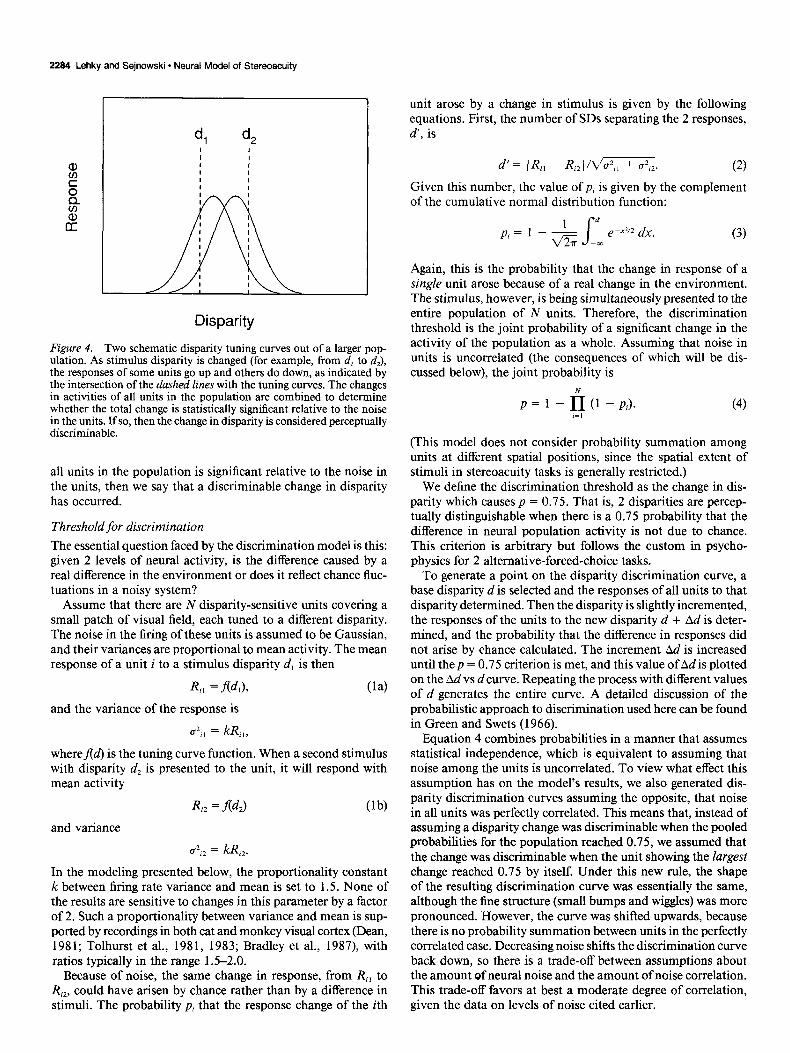
The concept underlying the stereoacuity model is outlined in Figure 4. It shows a subset of 2 disparity tuning curves from a much larger population. (In the actual model, the tuning curve shapes are somewhat different.) For disparity d,, both units have a particular response, indicated by the intersections of the dotted line with each of the tuning curves. When a different disparity, d,, is presented these responses both change, one increasing and the other decreasing. If the net change response summed over

2284 Lehky and Sejnowski - Neural Model of Stereoacuity

Disparity

Figure 4. Two schematic disparity tuning curves out of a larger population. As stimulus disparity is changed (for example, from d, to dJ, the responses of some units go up and others do down, as indicated by the intersection of the dashed lines with the tuning curves. The changes in activities of all units in the population are combined to determine whether the total change is statistically significant relative to the noise in the units. If so, then the change in disparity is considered perceptually discriminable.

all units in the population is significant relative to the noise in the units, then we say that a discriminable change in disparity has occurred.

Threshold for discrimination

The essential question faced by the discrimination model is this: given 2 levels of neural activity, is the difference caused by a real difference in the environment or does it reflect chance fluc- tuations in a noisy system?

Assume that there are N disparity-sensitive units covering a small patch of visual field, each tuned to a different disparity. The noise in the firing of these units is assumed to be Gaussian, and their variances are proportional to mean activity. The mean response of a unit i to a stimulus disparity d, is then

R,, =.W,),

and the variance of the response is

(14

u*,, = kR,,,

wheref(d) is the tuning curve function. When a second stimulus with disparity d, is presented to the unit, it will respond with mean activity

and variance

R,z = f(4) (lb)

azi2 = kR,,.

In the modeling presented below, the proportionality constant k between firing rate variance and mean is set to 1.5. None of the results are sensitive to changes in this parameter by a factor of 2. Such a proportionality between variance and mean is supported by recordings in both cat and monkey visual cortex (Dean, 1981; Tolhurst et al., 1981, 1983; Bradley et al., 1987), with ratios typically in the range 1.5-2.0.

Because of noise, the same change in response, from Ri, to R,2, could have arisen by chance rather than by a difference in stimuli. The probability p, that the response change of the ith

unit arose by a change in stimulus is given by the following equations. First, the number of SDS separating the 2 responses, d’, is

d’= (R,, - R,,//m.

Given this number, the value of p, is given by the complement of the cumulative normal distribution function:

p,=l- --& -1 e-x2/2 dx. s (3)

Again, this is the probability that the change in response of a single unit arose because of a real change in the environment. The stimulus, however, is being simultaneously presented to the entire population of N units. Therefore, the discrimination threshold is the joint probability of a significant change in the activity of the population as a whole. Assuming that noise in units is uncorrelated (the consequences of which will be discussed below), the joint probability is

N p = 1 - n (1 - p,).

,=I

(This model does not consider probability summation among units at different spatial positions, since the spatial extent of stimuli in stereoacuity tasks is generally restricted.)

We define the discrimination threshold as the change in disparity which causes p = 0.75. That is, 2 disparities are perceptually distinguishable when there is a 0.75 probability that the difference in neural population activity is not due to chance. This criterion is arbitrary but follows the custom in psychophysics for 2 alternative-forced-choice tasks.

To generate a point on the disparity discrimination curve, a base disparity d is selected and the responses of all units to that disparity determined. Then the disparity is slightly incremented, the responses of the units to the new disparity d + Ad is determined, and the probability that the difference in responses did not arise by chance calculated. The increment Ad is increased until the p = 0.75 criterion is met, and this value of Ad is plotted on the Ad vs d curve. Repeating the process with different values of d generates the entire curve. A detailed discussion of the probabilistic approach to discrimination used here can be found in Green and Swets (1966).

Equation 4 combines probabilities in a manner that assumes statistical independence, which is equivalent to assuming that noise among the units is uncorrelated. To view what effect this assumption has on the model’s results, we also generated disparity discrimination curves assuming the opposite, that noise in all units was perfectly correlated. This means that, instead of assuming a disparity change was discriminable when the pooled probabilities for the population reached 0.75, we assumed that the change was discriminable when the unit showing the largest change reached 0.75 by itself. Under this new rule, the shape of the resulting discrimination curve was essentially the same, although the fine structure (small bumps and wiggles) was more pronounced. However, the curve was shifted upwards, because there is no probability summation between units in the perfectly correlated case. Decreasing noise shifts the discrimination curve back down, so there is a trade-off between assumptions about the amount of neural noise and the amount of noise correlation. This trade-off favors at best a moderate degree of correlation, given the data on levels of noise cited earlier.

The Journal of Neuroscience, July 1990. fO(7) 2285

Model of disparity tuning curves

The first step in applying the model is to assign a mathematical form to the disparity tuning curves. We do not attempt to describe how these disparity-tuned properties are synthesized from monocular units. Furthermore, no attempt is made to describe the matching process between images to the 2 eyes or what aspects of the images may act as tokens during matching.

Following the classification of Poggio (1984) model tuning curves are divided into 3 classes: near, far, and tuned. The equation for the response of a “tuned” unit is

R = 1.5 exp[ -(d - d,,,)Va*] - 0.5 exp[-(d - d,,$/(2@], (5)

which is illustrated in Figure 5b. This is the difference of 2 Gaussian curves, one broader than the other, whose peaks are at the same position. Although tuned-inhibitory units are also observed experimentally, only tuned-excitatory units are used in the model because it is the magnitude of change and not its polarity that is relevant when determining discriminability. For the purposes of this model, therefore, both types of tuned units are equivalent. The equation for a “near” unit is

R = l.l3(exp[-(d - d,,&a2] - exp[-(d - (d,,, + u))Vcr2 - 1.01)

and the equation for its mirror image, a “far” unit, is

(6)

R = l.l3(exp[-(d - dpeaJ2/u2] - exp[(d - (d,,, - u))Vu2 - 1 .O]). (7)

Examples of these curves are shown in Figure 5, a, c. The asymmetries of the “near” and “far” tuning curves result from shifting the peaks of the 2 Gaussians by an amount c prior to subtracting them.

All 3 classes of curves have positive and negative lobes, which indicate modulation around a spontaneous level of activity, marked by the dashed zero lines in Figure 5. However, when actually performing calculations, the tuning curves were shifted up by 0.3 to eliminate negative values and renormalized to have a peak activity of 1.0.

Calculations of disparity threshold curves

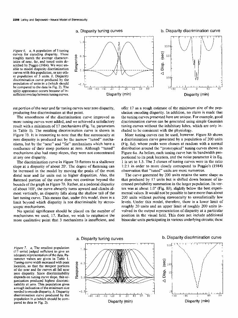
The task now is to find a set of tuning curves that generate a disparity discrimination curve resembling the psychophysical data (Fig. 2) within the constraints imposed by the physiology. We first tried, unsuccessfully, to do this with just 3 tuning curves (Fig. 6a), one from each class, which were selected with values of dpeak and u corresponding to average curves described by

Figure 5. Examples of model disparity tuning curves. a, Near unit; b, “tuned” unit; c, far unit. Their shapes resemble those described by Poggio (1984). Populations of disparity-tuned units are formed by vary- ing 2 parameters, one defining peak location and the other defining tuning bandwidth (Eqs. 5-7). The model does not depend on having these exact shapes, nor does it require them to be split into discrete classes.

Poggio (1984). The resulting discrimination curve (Fig. 6b) was entirely unsatisfactory. The prominent spikes occur because there was insufficient overlap between mechanisms. The situation could be alleviated somewhat by ignoring physiological constraints on tuning bandwidths and choosing a set of 3 curves giving the smoothest possible curve (that is, expand the width of the “tuned” mechanism so that its steepest portions coincide with the peaks of the “near” and “far” mechanisms). Though better, the resulting discrimination curve was still not satisfactory because it had a broad U-shape rather than the sharp V-shape found experimentally.

nificant change in shape) to levels indicated by the psychophysics. However, that amount of noise is much less than that measured physiologically. Another way to shift the curve down would be to increase the size of the population, because of probability summation (Eq. 4); i.e., since probability summation is being carried out over more units, a smaller difference in disparity leads to a statistically significant change in the pooled activity. This argument suggests that there must be more than 3 units engaged in encoding disparity at a particular location in the visual field. Furthermore, the additional units should have a range of different tuning curves to deal with problems in the discrimination curve shape discussed in the previous paragraph.

Another problem was that the curve in Figure 6b was too The next step was to add additional tuning curves to the high, not dropping below a discrimination threshold of 70”. population. After various attempts, we found the following rule: Decreasing the noise parameter k in Eq. 1 from 1.5 to 0.02 make the bandwidth of each tuning curve proportional to the shifted the disparity discrimination curve down (without sig- disparity of the tuning curve peak. This always placed the steep-

-0.5- near I I I I I I I I /

-80 -60 -40 -20 0 20 40 60 80

-0.5- tuned I I I I I I I I I I1 I I I

-80 -60 -40 -20 0 20 40 60 80

Disparity (min)


Figure 6. a, A population of 3 tuning curves for encoding disparity. These roughly match the average characteristics of near, far, and tuned units described by Poggio (1984). We were un- able to model disparity discrimination curves with this population, or any other population of 3 units. b, Disparity discrimination curve produced by the population of units in a (which should be compared to the data in Fig. 2). The spiky appearance occurs because of insufficient overlap between tuning curves.

a. Disparity tuning curves I r I ‘, / 1 I I r I r I( II

l.O-

c 4 -0.51, , , , , , ( , , , , , , ,j

-80 -60 -40 -20 0 20 40 60 80

Disparity (min)

b. Disparity discrimination curve

Disparity (min)

est portion of the near and far tuning curves near zero disparity, producing fine discrimination at that point.

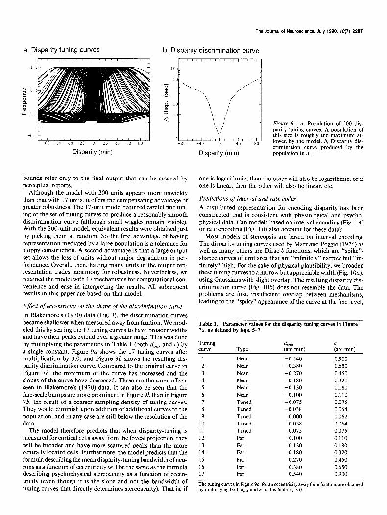
The smoothness of the discrimination curve improved as more tuning curves were added, and we achieved a satisfactory result with a minimum of 17 mechanisms (Fig. 7~2, parameters in Table 1). The resulting discrimination curve is shown in Figure 7b. It is interesting to note that the fine stereoacuity at zero disparity is produced not by the narrow “tuned” mechanisms, but by the “near” and “far” mechanisms which have a confluence of their steep portions at zero. Although “tuned” mechanisms also had steep slopes, they were not concentrated at any one disparity.

The discrimination curve in Figure 7b flattens to a shallower slope at a disparity of about 20’. The degree of flattening can be increased in the model by moving the peaks of the most distal near and far units out to higher disparities. Also, the flattened portion of the curve does not continue beyond the bounds of the graph in Figure 7b. Rather, at a pedestal disparity of about loo’, the curve abruptly turns upward and climbs almost vertically, as disparity falls along the shallow tail of the last tuning curve. This means that, under this model, there is a limit beyond which disparity is not discriminable by stereoscopic mechanisms.

No special significance should be placed on the number of mechanisms we used, 17. Rather, we wish to emphasize the more qualitative point that 3 mechanisms is insufficient, and

offer 17 as a rough estimate of the minimum size of the population encoding disparity. In addition, no claim is made that the tuning curves presented here are unique. For example, good discrimination curves can be generated using simple Gaussian tuning curves without the inhibitory lobes, which are only included to be consistent with the physiology.

More tuning curves can be used, however. Figure 8b shows a discrimination curve generated by a population of 200 units (Fig. 8a), whose peaks were chosen at random with a normal distribution around the “prototypical” tuning curves shown in Figure 6a. As before, each tuning curve has its bandwidth proportional to its peak location, and the noise parameter k in Eq. 1 is set to 1.5. The 3 classes of tuning curves were in the ratio 1:2: 1 in order to more closely correspond to Poggio’s (1984) observation that “tuned” units are most numerous.

The curve generated by 200 units retains the same shape as that produced by 17 units but is shifted down because of increased probability summation in the larger population. Its vertex was at about 1.0” (Fig. 8b), slightly below the best experimental values. It would not be possible to have more than about 200 units without pushing stereoacuity to unrealistically low levels. Under this model, therefore, there is a lower limit of roughly 20 units and an upper limit of roughly 200 units involved in the output representation of disparity at a particular position in the visual field. This does not include additional binocular units participating in various underlying circuits; these

Figure 7. a, The smallest population (17 units) judged sufficient to give an adequate representation ofthe data. Pa- rameter values are given in Table 1. Tuning curve width increased with peak location, so that the steepest portions of the near and far curves all fall near zero disparity. Since discriminability depends on tuning curve slope, this organization produced highest discriminability at zero. This population gives a rough indication of the minimum size needed to encode disparity. b, Disparity discrimination curve produced by the population in a (which should be compared to data in Fig. 2).

a. Disparity tuning curves

-0.5

-80 -60 -40 -20 0 20 40 60 80

Disparity (min)


lo- -80 -40 0 40 80

Disparity (min)

The Journal of Neuroscience, July 1990, W(7) 2287


I”““““““““‘1

-o.st, , , , , , , , , , , ( , , , , j

-80 -60 -40 -20 0 20 40 60 80


I”“““““““’

Disparity (min)

bounds refer only to the final output that can be assayed by perceptual reports.

Although the model with 200 units appears more unwieldy than that with 17 units, it offers the compensating advantage of greater robustness. The 17-unit model required careful fine tuning of the set of tuning curves to produce a reasonably smooth discrimination curve (although small wiggles remain visible). With the 200-unit model, equivalent results were obtained just by picking them at random. So the first advantage of having representation mediated by a large population is a tolerance for sloppy construction. A second advantage is that a large output set allows the loss of units without major degradation in per- formance. Overall, then, having many units in the output representation trades parsimony for robustness. Nevertheless, we retained the model with 17 mechanisms for computational con- venience and ease in interpreting the results. All subsequent results in this paper are based on that model.

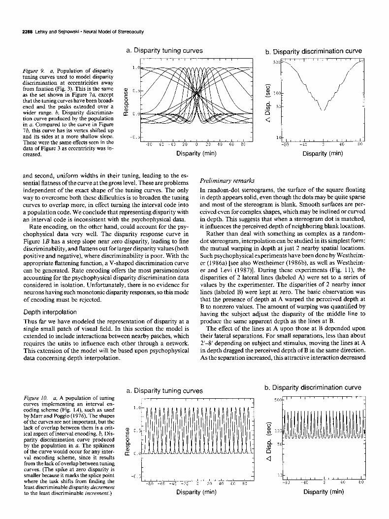
Effect of eccentricity on the shape of the discrimination curve In Blakemore’s (1970) data (Fig. 3), the discrimination curves became shallower when measured away from fixation. We modeled this by scaling the 17 tuning curves to have broader widths and have their peaks extend over a greater range. This was done by multiplying the parameters in Table 1 (both dFal, and a) by a single constant. Figure 9a shows the 17 tuning curves after multiplication by 3.0, and Figure 9b shows the resulting disparity discrimination curve. Compared to the original curve in Figure 7b, the minimum of the curve has increased and the slopes of the curve have decreased. These are the same effects seen in Blakemore’s (1970) data. It can also be seen that the fine-scale bumps are more prominent in Figure 9b than in Figure 7b, the result of a coarser sampling density of tuning curves. They would diminish upon addition of additional curves to the population, and in any case are still below the resolution of the data.

The model therefore predicts that when disparity-tuning is measured for cortical cells away from the fovea1 projection, they will be broader and have more scattered peaks than the more centrally located cells. Furthermore, the model predicts that the formula describing the mean disparity-tuning bandwidth ofneu- rons as a function of eccentricity will be the same as the formula describing psychophysical stereoacuity as a function of eccentricity (even though it is the slope and not the bandwidth of tuning curves that directly determines stereoacuity). That is, if

Disparity (min)

Figure 8. a, Population of 200 disparity tuning curves. A population of this size is roughly the maximum allowed by the model. b, Disparity discrimination curve produced by the population in a.

one is logarithmic, then the other will also be logarithmic, or if one is linear, then the other will also be linear, etc.

Predictions of interval and rate codes A distributed representation for encoding disparity has been constructed that is consistent with physiological and psychophysical data. Can models based on interval encoding (Fig. 1A) or rate encoding (Fig. 1B) also account for these data?

Most models of stereopsis are based on interval encoding. The disparity tuning curves used by Marr and Poggio (1976) as well as many others are Dirac 6 functions, which are “spike”- shaped curves of unit area that are “infinitely” narrow but “infinitely” high. For the sake of physical plausibility, we broaden these tuning curves to a narrow but appreciable width (Fig. lOa), using Gaussians with slight overlap. The resulting disparity discrimination curve (Fig. lob) does not resemble the data. The problems are first, insufficient overlap between mechanisms, leading to the “spiky” appearance of the curve at the fine level,

Table 1. Parameter values for the disparity tuning curves in Figure 7a, as defined by Eqs. 5-7

Tuning d curve Type (E min) [arc min)

1 Near -0.540 0.900 2 Near -0.380 0.650 3 Near -0.270 0.450 4 Near -0.180 0.320 5 Near -0.130 0.180 6 Near -0.100 0.110 7 Tuned -0.075 0.075 8 Tuned -0.038 0.064 9 Tuned 0.000 0.062

10 Tuned 0.038 0.064 11 Tuned 0.075 0.075 12 Far 0.100 0.110 13 Far 0.130 0.180 14 Far 0.180 0.320 15 Far 0.270 0.450 16 Far 0.380 0.650 17 Far 0.540 0.900

The tuning curves in Figure 9~2, for an eccentricity away from fixation, are obtained by multiplying both dpak and CJ in this table by 3.0.


Figure 9. a, Population of disparity tuning curves used to model disparity discrimination at eccentricities away from fixation (Fig. 3). This is the same as the set shown in Figure 7a, except that the tuning curves have been broad- ened and the peaks extended over a wider range. b, Disparity discrimination curve produced by the population in a. Compared to the curve in Figure lb, this curve has its vertex shifted up and its sides at a more shallow slope. These were the same effects seen in the data of Figure 3 as eccentricity was increased.


L

-0.5 I I I I, I I, I I,

-80 -60 -40 -20 0 20 40 60 80

Disparity (min)

and second, uniform widths in their tuning, leading to the essential flatness of the curve at the gross level. These are problems independent of the exact shape of the tuning curves. The only way to overcome both these difficulties is to broaden the tuning curves to overlap more, in effect turning the interval code into a population code. We conclude that representing disparity with an interval code is inconsistent with the psychophysical data.

Rate encoding, on the other hand, could account for the psychophysical data very well. The disparity response curve in Figure 1B has a steep slope near zero disparity, leading to fine discriminability, and flattens out for larger disparity values (both positive and negative), where discriminability is poor. With the appropriate flattening function, a V-shaped discrimination curve can be generated. Rate encoding offers the most parsimonious accounting for the psychophysical disparity discrimination data considered in isolation. Unfortunately, there is no evidence for neurons having such monotonic disparity responses, so this mode of encoding must be rejected.

Depth interpolation

Thus far we have modeled the representation of disparity at a single small patch of visual field. In this section the model is extended to include interactions between nearby patches, which requires the units to influence each other through a network. This extension of the model will be based upon psychophysical data concerning depth interpolation.

Figure 10. a, A population of tuning curves implementing an interval encoding scheme (Fig. lA), such as used by Marr and Poggio (1976). The shapes of the curves are not important, but the lack of overlap between them is a crit- ical aspect of interval encoding. b, Dis- parity discrimination curve produced by the population in a. The spikiness of the curve would occur for any interval encoding scheme, since it results from the lack of overlap between tuning curves. (The spike at zero disparity is smaller because it marks the splice point where the task shifts from finding the least discriminable disparity decrement to the least discriminable increment.)


-80 -40 0 40 80

Disparity (min)

Preliminary remarks

In random-dot stereograms, the surface of the square floating in depth appears solid, even though the dots may be quite sparse and most of the stereogram is blank. Smooth surfaces are perceived even for complex shapes, which may be inclined or curved in depth. This suggests that when a stereogram dot is matched, it influences the perceived depth of neighboring blank locations.

Rather than deal with something as complex as a random- dot stereogram, interpolation can be studied in its simplest form: the mutual warping in depth at just 2 nearby spatial locations. Such psychophysical experiments have been done by Westheim- er (1986a) [see also Westheimer (1986b), as well as Westheim- er and Levi (1987)]. During these experiments (Fig. 1 l), the disparities of 2 lateral lines (labeled A) were set to a series of values by the experimenter. The disparities of 2 nearby inner lines (labeled B) were kept at zero. The basic observation was that the presence of depth at A warped the perceived depth at B to nonzero values. The amount of warping was quantified by having the subject adjust the disparity of the middle line to produce the same apparent depth as the lines at B.

The effect of the lines at A upon those at B depended upon their lateral separations. For small separations, less than about 2’-8’ depending on subject and stimulus, moving the lines at A in depth dragged the perceived depth of B in the same direction. As the separation increased, this attractive interaction decreased


C’ I / ““I “““““I

1 I I1 ( I I , I I

-80 -60 -40 -20 0 20 40 60 80

Disparity (min) Disparity (min)


5oom

lob,, , , , , , / , , , , , , , , ,I -80 -40 0 40 80

The Journal of Neuroscience, July 1990, 1 O(7) 2289

0

0

Figure Il. Schematic of the setup used by Westheimer (1986a) to measure lateral interactions between nearby stimuli at different depths. The circles represent lines seen by the observer. When the outer lines A were moved in depth, the apparent depth of the nearby lines B were dragged along with them, although the physical disparities of B remained unchanged. For small spatial separations between A and B, B was dragged in the same direction as A (attraction), and for larger separations, B was repulsed. The central line was used to monitor the apparent depth at B.

and then reversed so that the 2 lines appeared to repel each other. That is, as the lines at A moved back in depth, the lines at B appeared to move forward. This repulsive effect extended over a much broader spatial range than the attractive effect. Repulsion was still evident at the maximum lateral separation tested, 12’.

Network model: qualitative aspects

The opponent spatial organization of depth attraction and repulsion in Westheimer’s psychophysical data immediately suggests an old idea in neuroscience: short-range excitation and long-range inhibition between neurons (Ratliff, 1965). That is what our model will implement.

Assume that the entire population of 17 disparity-tuned units used previously (Fig. 7a) is replicated at each spatial location. A unit at one location interacts with units at neighboring locations to form a network. Assume further that a unit interacts only with other units (at different locations) tuned to the same disparity, as indicated in Figure 12. If units tuned to the same disparity are spatially close, there is mutual excitation, but if they are farther apart, there is inhibition. The modeling ofspatial interactions is only concerned with mean activities, so that the noise discussed in the discrimination modeling is no longer a factor.

Before proceeding, several points should be made about the network. First, it is worth emphasizing that no strong significance is placed on having exactly 17 mechanisms. This is just a minimum number that produced reasonable results in the discrimination modeling, and it is convenient to work with a minimal model. Second, although the model treats excitation as occurring between closely spaced units, other interpretations are possible. Alternatively, it may reflect stimulus summation within a single unit rather than mutual excitation between 2

Tuning Curve 1

Tuning curve 2

Tuning curve 17

Position A Position B

(disparity 1) (disparity 2)

l 0

l l

l l

Figure 12. Model configuration for producing depth attraction and repulsion. Disparity at each position was represented by a population of 17 disparity-tuned units (Fig. 74. There were lateral interactions between units at A and B tuned to the same disparity, which were excitatory if the separation between the 2 was small, and inhibitory if the separation was larger. There were no interactions between units at a single position.

units. Third, the assumption that only units tuned to the same disparity interact may be more restrictive than needed. There could also be weaker interactions with units tuned to other disparities, which taper offwith increasing difference in disparity tuning. Fourth, we assume that no interactions occur within the set of disparity-tuned mechanisms located at a single location. In the future it may be necessary to add such connections as the model is applied to other binocular phenomena.

Finally, when we say that there is a representation of disparity at each spatial position, we must be more precise about the term “position.” Each encoding population represents disparity for some patch of visual field. For present purposes, the size of these patches may be considered the area subserved by a single cortical column, but this is an empirical question, and in any case spatial scale does not affect the formal structure of the model. Similarly, the scale of the lateral interactions is also an empirical question. Therefore, units are described as being “close together” or “far apart,” and the specific values are left for experimental inves- tigation, although the psychophysical data suggests interactions confined to a radius of about a quarter to a third of a degree.

2290 Lehky and Sejnowski l Neural Model of Stereoacuity

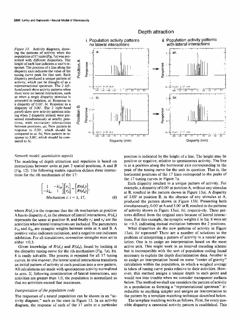
Figure 13. Activity diagrams, showing the patterns of activity when the population of 17 units (Fig. 7~) was presented with different disparities. The height of each line indicates a unit’s response. The position of a line along the disparity axis indicates the value of the tuning curve peak for that unit. Each disparity produced a unique pattern of activity, which can be thought of as a representational spectrum. The 2 left- handpanels show activity patterns when there were no lateral interactions, such as when a single disparity stimulus is presented in isolation. ai, Response to a disparity of 0.00’. bi, Response to a disparity of 3.00’. The 2 right-hand panels show new activity patterns arising when 2 disparity stimuli were presented simultaneously at nearby positions, with excitatory interactions between positions. aii, New pattern in response to O.OO’, which should be compared to ai. bii, New pattern in response to 3.00’, which should be compared to bi.

Depth attraction

i. Population activity patterns ii. Population activity patterns no lateral interactions with lateral interactions

-I t -0.5 ‘hsp: 0.00 mm -0.5 01sp: 1.00 InL” 18 I, 1, ( 11, / ,,,I,/,,,

-80 -60 -40 -20 0 20 40 60 80 -80 -60 -40 -20 0 20 40 60 80

-0.5~ lisp: 3.00 nun -80 -60 -40 -20 0 20 40 60 80

Disparity (min)

Network model: quantitative aspects The modeling of depth attraction and repulsion is based on interactions between units at just 2 spatial positions, A and B (Fig. 12). The following matrix equation defines these interactions for the ith mechanism of the 17:

Mechanism i: i = 1, 17, (8)

where I+(d,) is the response that the ith mechanism at position A has to disparity d, in the absence of lateral interactions, R(d,) represents the same at position B, and finally r,.,l and rBi are the activities when lateral interactions are included. The parameters ka, and kLA are synaptic weights between units at A and B. A positive value indicates excitation, and a negative one indicates inhibition. For all simulations, connection strengths were set to either kO.5.

Given knowledge of R’(d,J and R’(d,), found by looking at the disparity tuning curve for the ith mechanism (Fig. 7a), Eq. 8 is easily solvable. The process is repeated for all 17 tuning curves. In this manner, the lateral spatial interactions transform an initial pattern of activity at each position into a new pattern. All calculations are made with spontaneous activity normalized to zero. If, following consideration of lateral interactions, any activities are greater than 1 .O, the population is normalized so that no activities exceed that maximum.

Interpretation of the population code The responses of a neural population can be shown in an “activity diagram,” such as the ones in Figure 13. In an activity diagram, the response of each of the 17 units at a particular

3

-0.5 01sp: 2.10 ml" I I I I1 I I I 1 I

-80 -60 -40 -20 0 20 40 60 80

Disparity (min)

position is indicated by the height of a line. The height may be positive or negative, relative to spontaneous activity. The line is at a position along the horizontal axis corresponding to the peak of the tuning curve for the unit in question. That is, the horizontal positions of the 17 lines correspond to the peaks of the 17 tuning curves in Figure 7a.

Each disparity resulted in a unique pattern of activity. For example, a disparity of 0.00’ at position A, without any stimulus at B, resulted in the pattern shown in Figure 13ai. A disparity of 3.00’ at position B, in the absence of any stimulus at A, produced the pattern shown in Figure 13bi. Presenting both simultaneously, 0.00’ at A and 3.00’ at B, resulted in the patterns of activity shown in Figure 13aii, bii, respectively. These patterns differed from the original ones because of lateral interactions. For this example, the synaptic weights k in Eq. 8 were set to +0.5, indicating mutual excitation between the 2 positions.

What disparities do the new patterns of activity in Figure 13aii, bii represent? There are a number of solutions to the problem of interpreting a pattern of activity in a neural population. One is to assign an interpretation based on the most active unit. This might work in an interval encoding scheme but is incompatible with the sort of population coding found necessary to explain the depth discrimination data. Another is to assign an interpretation based on some “center of gravity” calculation within the population, in which a weighed average is taken of tuning curve peaks relative to their activities. How- ever, this method assigns a unique depth to each point and would run into trouble when we consider transparent surfaces below. The method we shall use considers the pattern of activity in a population as forming a “representational spectrum” ir- reducible to anything simpler and assigns an interpretation to the pattern by a template matching technique described below.

The template matching works as follows. First, for every possible disparity a canonical activity pattern is established. This

The Journal of Neuroscience, July 1990, fO(7) 2291

Depth attraction. Interpreting activity patterns

1.0 I / / I I I I

a.

Dlsp: 2.10 min I 0. o- / / I I, I I

-30 -20 -10 0 10 20 30

Disparity (min)

Figure 14. Root mean square (RMS) error curves used to assign an interpretation to the new patterns of activity in Figure 13aii, bii. The RMS difference between the new pattern and all possible canonical (i.e., unperturbed) patterns is calculated and plotted. The new pattern is assigned the disparity of the best-fit canonical pattern, indicated by the minimum of the RMS curve. a, RMS curve for the pattern shown in Figure 13aii. The minimum occurs at 1 .OO’, and the pattern in Figure 13aii is interpreted as representing that disparity. The vertical line shows the physical stimulus disparity (that of Fig. 13ai, 0.00’). Thus, lateral interactions have shifted the apparent disparity at this location from 0.00’ to 1.00’. b, The RMS curve for the pattern in Figure 13bii. The minimum RMS error occurs at an apparent disparity of 2.16’. The vertical line shows the physical stimulus disparity (that of Fig. 13bi, 3.00’).

canonical pattern is simply the pattern produced in the population when a disparity is presented in the absence of any per- turbing lateral influences. Figure 13ai, bi are canonical patterns for disparities 0.00’ and 3.00’, for example, because they are the responses to a single disparity stimulus without any lateral interactions. On the other hand, Figure 13aii, bii are not canonical patterns for any disparity because those precise patterns cannot be generated by any single disparity stimulus in isolation since they are affected by lateral perturbations.

Under template matching, an arbitrary activity pattern is assigned a disparity by finding which canonical pattern matches it best. A variety of matching rules can be used. We have chosen to minimize the root-mean-square (RMS) error between the arbitrary patterns and the canonical patterns, with the RMS error determined for the population as a whole. This matching procedure is just a formalism of the model, and we do not expect that it literally occurs in the brain; there is, ofcourse, no evidence for neural circuits calculating RMS errors. It is intended to

I I 4- a.

l No interaction 0

3- Excitatory interaction .

-2 - 4 0

I I 4-b. 0

l NO interaction o Inhibitory t

3- interaction . -z _ .-

.E. 2- %

.E 1

x, - 2 O- . n

_ 4

-l- 0

Spatial Position

Figure 15. a, Summary of the results in Figures 13 and 14. Black dots show the original disparities when each of the 2 stimuli was presented individually (Fig. 13ai, bi). White dots show the new, apparent disparities (Fig. 13aii, bii, as interpreted by Fig. 14, a, b), arising from interactions between simultaneously presented stimuli. The excitatory interactions produced an apparent attraction between the disparities. b, Summary of results when the procedures shown in Figures 13 and 14 were carried out with inhibitory interactions rather than excitatory ones. In this case, the disparities show an apparent repulsion.

mirror the results of the pattern interpretation process in the brain, and not the actual process itself.

Depth attraction and repulsion between 2 locations

The template method will be applied to determine the disparities represented by the 2 activity patterns shown on the right in Figure 13. For Figure 13aii, the RMS error between that pattern and all possible canonical patterns is calculated, and plotted in Figure 14~. The minimum of this graph indicates that Figure 13aii most closely matches the canonical pattern for 1 .OO’. We say, then, that the neural activity shown in Figure 13aii represents the disparity 1 .OO’ and is responsible for producing the sensation of that depth. Followingthe same procedure for Figure 13bii (with RMS errors plotted in Fig. 14b), that pattern is interpreted as representing the disparity 2.10’.

The results in Figures 13 and 14 are summarized in Figure 15~. It shows that mutual excitation between 2 positions causes an “attractive” effect in the apparent disparities at both positions. At position A, the disparity has shifted up from 0.00’ to 1 .OO’, and at position B, it has shifted down from 3.00’ to 2.10’. On the other hand, if the interactions are inhibitory, then there is a “repulsive” effect, as shown in Figure 15b. (The activity diagrams and RMS curves for the inhibitory case are not shown.)

In the psychophysical experiments described earlier, Westhei- mer (1986a) found depth attraction between 2 stimuli when they were spatially close and repulsion when they were further


I I I I I , ), I I t I I I I1 I -1000 -500 0 500 1000

Disparity (set)

Figure 16. Stereo interpolation data (black dots) from Westheimer (1986a) based on the experimental setup in Figure 11. The apparent shift in disparity at B is shown as a function of a real shift in the disparity at A. This line shows predictions of the model.

apart. These effects are duplicated in the model by using excitatory connections to produce the short-range depth attraction or inhibitory connections to produce the longer-range depth repulsion.

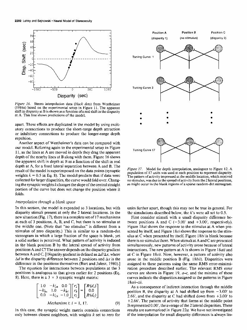
Another aspect of Westheimer’s data can be compared with our model. Referring again to the experimental setup in Figure 11, as the lines at A are moved in depth they drag the apparent depth of the nearby lines at B along with them. Figure 16 shows the apparent shift in depth at B as a function of the shift in real depth at A, for a fixed lateral separation between A and B. The result of the model is superimposed on the data points (synaptic weights k = 0.5 in Eq. 8). The model predicts that if data were collected for larger disparities, the curve would fold over. Chang- ing the synaptic weights k changes the slope of the central straight portion of the curve but does not change the position where it folds.

Interpolation through a blank space In this section, the model is expanded to 3 locations, but with disparity stimuli present at only the 2 lateral locations. In the new situation (Fig. 17), there is a complete set of 17 mechanisms at each of 3 positions, A, B, and C, but there is no stimulus at the middle one. (Note that “no stimulus” is different from a stimulus of zero disparity.) This is similar to a random-dot stereogram in which a large fraction of the space is blank, yet a solid surface is perceived. What pattern of activity is induced in the blank position B by the lateral spread of activity from positions A and C? The answer depends on the disparity gradient between A and C. [Disparity gradient is defined as Ad/Ax, where Ad is the disparity difference between 2 positions and Ax is the difference in the positions themselves (Burt and Julesz, 1980).]

The equation for interactions between populations at the 3 positions is analogous to that given earlier for 2 positions (Eq. 8). Here, there is a 3 x 3 synaptic weight matrix:

[$J 2: ~~;l[~]=~.~]

Mechanism i: i = 1, 17. (9)

In this case, the synaptic weight matrix contains connections only between closest neighbors, with weights k set to zero for

Position A Position B

(disparity 1) (no stimulus)

Position C

(disparity 2)

Tuning Curve 1

Tuning Curve 2

.

.

.

. .

. .

. .

Tuning Curve 17

Figure 17. Model for depth interpolation, analogous to Figure 12. A population of 17 units was used at each position to represent disparity. The pattern of activity impressed at the middle location, which received no stimulus, was due to the spread of activity from the 2 lateral positions, as might occur in the blank regions of a sparse random-dot stereogram.

units further apart, though this may not be true in general. For the simulations described below, the k’s were all set to 0.5.

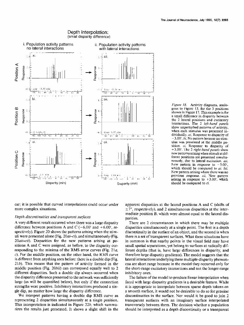
First consider stimuli with a small disparity difference between positions A and C (-3.00’ and +3.00’, respectively). Figure 18ai shows the response to the stimulus at A when presented by itself, and Figure 18ci shows the response to the stimulus at C when presented by itself. Figure 18bi is blank because there is no stimulus there. When stimuli at A and C are presented simultaneously, new patterns of activity arose because of lateral interactions. The new pattern at A is shown in Figure 18aii and at C in Figure l&ii. Now, however, a pattern of activity also arose in the middle position B (Fig. 18bii). Disparities were assigned to these patterns using the same RMS error-minimi- zation procedure described earlier. The relevant RMS error curves are shown in Figure 19, a-c, and the minima of these curves indicate the disparities assigned to the patterns in Figure 18aii-cii.

As a consequence of indirect interaction through the middle position B, the disparity at A had shifted up from -3.00’ to 2.66’, and the disparity at C had shifted down from +3.00’ to +2.66’. The pattern of activity that forms at the middle point B represented O.OO’, the average of the 2 lateral disparities. These results are summarized in Figure 22a. We have not investigated if the interpolation for small disparity differences is always lin-

The Journal of Neuroscience, July 1990, IO(7) 2293

Depth interpolation: (small disparity difference)

i. Population activity patterns no lateral interactions

I’ ” ” ” “’ 1 ” ” ” 1

ii. Population activity patterns with lateral interactions

1 L Figure 18. Activity diagrams, analogous to Figure 13, for the 3 positions shown in Figure 17. This example is for a small difference in disparity between the 2 lateral positions and excitatory interactions. The 2 left-hand panels show unperturbed patterns of activity, when each stimulus was presented individually. ai, Response to disparity of -3.00’. bi, No pattern because no stimulus was presented at the middle position. ci, Response to disparity of +3.00’. The 2 right-hand panels show new patterns arising when stimuli at different positions are presented simultaneously, due to lateral excitation. aii, New pattern in response to -3.00’, which should be compared to ai. bii, New pattern arising where there was no previous response. cii, New pattern arising in response to +3.00’, which should be compared to ci.

ear; it is possible that curved interpolations could occur under more complex situations.

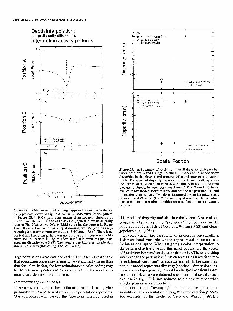
Depth discontinuities and transparent surfaces A very different result occurred when there was a large disparity difference between positions A and C (-6.00’ and +6.00’, respectively). Figure 20 shows the patterns arising when the stimuli were presented alone (Fig. 20ai-ci), and simultaneously (Fig. 20aikii). Disparities for the new patterns arising at positions A and C were assigned, as before, to the disparity corresponding to the minima of the RMS error curves (Fig. 21a, c). For the middle position, on the other hand, the RMS curve is different from anything seen before: there is a double dip (Fig. 21b). This means that the pattern of activity formed in the middle position (Fig. 20bii) can correspond equally well to 2 different disparities. Such a double dip always occurred when the disparity difference presented to the network was sufficiently large (as will be quantified below), but only if the connection strengths were positive. Inhibitory interactions produced a single dip, no matter how large the disparity difference.

We interpret patterns having a double dip RMS curve as representing 2 disparities simultaneously at a single position. This interpretation is indicated in Figure 22b, which summa- rizes the results just presented. It shows a slight shift in the

apparent disparities at the lateral positions A and C (shifts of If-7”, respectively), and 2 simultaneous disparities at the intermediate position B, which were almost equal to the lateral disparities.

There are 2 circumstances in which there may be multiple disparities simultaneously at a single point. The first is a depth discontinuity in the surface of an object, and the second is when there is a set of transparent surfaces. What these situations have in common is that nearby points in the visual field may have small spatial separations, yet belong to surfaces at radically different depths (that is, have large differences in disparity, and therefore large disparity gradients). The model suggests that the lateral interactions underlying these multiple-disparity phenomena are short range because in the model they occurred only for the short-range excitatory interactions and not the longer-range inhibitory ones.

The failure of the model to produce linear interpolation when faced with large disparity gradients is a desirable feature. While it is appropriate to interpolate between sparse depth tokens on a smooth surface, it would not be desirable to do so for genuine discontinuities in the surface. Nor would it be good to join 2 transparent surfaces with an imaginary surface interpolated transversely between them. The decision whether a population should be interpreted as a depth discontinuity or a transparent


Depth interpolation: (small disparity difference).

Interpreting activity patterns

ante of transparency. The disparity difference at the transition from averaging to transparency increased as a function of the mean disparity of the 2 sets of dots. The transition was gradual, in which the surface appeared roughened and thickened before

l.O a. I I I , I I /

I

Dlsp: -2.64 min I 0.0 I I I I/ I I 1

-30 -20 -10 0 10 20 30

/ , I , , / /

“‘- b.

01s~: 0.00 min 0.0 I I I I / I /

-30 -20 -10 0 10 20 30

Disp: ̂ ‘” ‘- 0.0 I

-30

Disparity (min)

Figure 19. RMS curves, analogous to those of Figure 14, used to assign disparity interpretations to the activity patterns in Figure 18aii-cii. a, RMS curve for the pattern in Figure 18aii. The RMS minimum assigns that pattern an apparent disparity of -2.64’, and the vertical line&- dicates the physical stimulus disnaritv (that of Fig. 18ai. -3.00’). b. RMS curve for the pattern in Figure 1 &ii. The RMS minimum assigns it an apparent disparity of 0.00’. There is no vertical line here because there was no stimulus at this position. c, RMS curve for the pattern in Figure 18cii. RMS minimum assigns it an apparent disparity of +2.64’. The vertical line indicates the physical stimulus disparity (that of Fig. 18ci, +3.00’).

surface is likely to be made at a more global level than considered in this model, for there is little information available locally to distinguish between the 2 possibilities.

The central premise of the model was that disparity is encoded by a population of units having broad, overlapping tuning curves. In such a distributed representation, the activity of a single unit gives only a coarse indication of the stimulus parameter. This does not mean that precise information is lost, but only that the information is dispersed over a pattern of activity in the population. Other ways of representing disparity were also considered, namely, interval encoding, in which a separate unit is dedicated to each small range of disparity, and rate encoding, in which disparity is proportional to the firing rate of a single unit. Both of these schemes were found to be inconsistent with the physiological or psychophysical data.

A transition from depth averaging to transparency has been The concept of distributed representations arose in nineteenth observed psychophysically by Parker and Yang (1989). They century psychophysics with the idea that color is encoded by measured the depth percept that resulted when random-dot ster- the relative activities in a population of 3 overlapping color eograms were constructed by intermixing dots from 2 depth channels. In our model, the parameter is “disparity” rather than planes. For small disparity differences, the percept was ofa single “color,” and more mechanisms were required to explain the surface at the average of the 2 depths, but for large differences, data, but the essence of the idea is the same. In a similar manner, the percept was that of 2 simultaneous depths and the appear- it is possible to apply the concept to many other parameters.

it broke into 2 transparent surfaces. The transition between averaging and transparency in our

model occurs at the disparity difference for which the RMS error curve goes from one dip (as in Fig. 196) to 2 dips (as in Fig. 2 1 b). The following procedure was used to find this disparity. Starting with equal disparities at A and C, the disparity at A was decreased and that at C increased by an equal amount, so that mean disparity, (dA + dJ2, remained constant but the disparity difference, 1 d, - dc 1, increased. The smallest difference producing 2 equal dips was defined as the onset of transparency. It should be pointed out that the single dip does not suddenly break into 2 equal dips, except for the case of sym- metrical modulation about zero mean disparity. Rather, the second dip starts as a small outpouching which grows as the disparity difference increases, until both become equal. There- fore, our criterion for the appearance of transparency is the end point of a gradual transition.

The disparity difference required to produce transparency in the model increased rapidly with mean disparity (Fig. 23). This is also a feature of the data of Parker and Yang (1989). While the modeling and data curves are qualitatively similar in shape, the model curve is shifted up by a factor of 4. The reason for this is not known. Changing synaptic weights k in Eq. 9 over a reasonable range does not appreciably affect transparency onset in the model, nor can the differences be explained by criterion differences in judging the onset of transparency. One possibility is that the large, 2-dimensional random-dot patterns used by Parker and Yang (1989) lead to lower transparency-onset thresholds than the small, l-dimensional patterns considered in the model.

Discussion

We have had 2 goals. The first was to constrain possible mechanisms of stereopsis by modeling a variety of other binocular phenomena, in continuation with previous models on binocular brightness summation (Lehky, 1983) and binocular rivalry (Leh- ky, 1988). The second was to provide a general framework for population coding models which may be applicable by analogy to other neural parameters unrelated to binocular vision.

The Journal of Neuroscience, July 1990, W(7) 2295

Depth interpolation: (large disparity difference)

i. Population activity patterns ii. Population activity patterns no lateral interactions with lateral interactions

1’1’1’ 1 “’ 1 ‘I I’ 1 1 ‘.I

m Figure 20. Activity diagram for 3 in- teracting locations (Fig. 17) but with a large difference in disparities at the 2 lateral positions instead ofthe small difference shown in Figure 18. Left column shows unperturbed patterns of activity. ai, Response to disparity of -6.00’. bi, No pattern because no stimulus was presented at the middle position. ci, Response to disparity of +6.00’. Right column shows new patterns arising when stimuli at different locations were presented simultaneously, with lateral interactions. aii, New pattern in response to -6.00’, which should be compared to ai. bii, New pattern arising where there was no pre-

-0.5 5 88 min vious response. cii, New pattern arising -illl -6C -4” -20 0 20 40 60 80 in to +6.00’, which should be response

Disparity (min) compared to ci.

Examples of this are models incorporating a population code for the visual representation of stimulus size (Gelb and Wilson, 1983), and for the motor representation of arm movements (Georgopolous et al., 1986).

Since this model is concerned in part with the representation of transparent stimuli, it is possible that analogous models can be constructed for other transparency phenomena besides those arising from depth. A specific example involves motion. Adel- son and Movshon (1982) studied the percept of 2 superimposed gratings drifting in different directions and found conditions under which they “cohered” to form a single drifting plaid, or alternatively appeared as 2 transparent surfaces sliding over each other, depending on how similar the 2 gratings were in various respects (speed, spatial frequency, contrast, etc.). This appears analogous to the transition from depth averaging to transparency discussed earlier, and perhaps it can be understood in terms of a distributed representation for motion formally analogous to the one used for disparity here.

Some consequences of population coding were analyzed by Hinton et al. (1986) in the context of model neurons allowed to have only 2 levels of firing, fully on or fully OK This allows a parameter to be encoded by a set of overlapping, rectangular- shaped tuning curves. Using binary-valued units rather than continuously valued units, as used here, leads to differences about how limits to discriminability arise. In Hinton’s model,

which does not include noise, the accuracy with which information is encoded is determined by the number of rectangular tuning-curve boundaries crossed as the parameter’s value is changed. As formulated by Hinton, this is a function of both the number and widths of the tuning curves. The situation is very different for a population of continuous-valued units. For this case, in the absence of noise a parameter’s value can be encoded with infinite precision independent of the number and widths of the tuning curves. Discriminability in a population of continuously valued units is limited by the amount of noise and the slopes of the tuning curves, and not the widths of the tuning curves.

Our model leads to the conclusion that the population size encoding disparity for a small patch of visual field may be as small as a few tens of units or as large as a few hundred. This is much larger than the 3 found in color vision, which is the best established example of population coding. However, the small size of the color representation may be unusual. Having a large number of color mechanisms requires the burden of maintaining separate genes for each type of pigment molecule (Nathans et al., 1986). In contrast, there appears to be less cost in providing a broad range of values for other visual parameters, which may involve gradations in the biophysical or anatomical characteristics of the underlying neurons. Some of the advan- tages of building redundancy into a representation by having

2299 Lehky and Sejnowski - Neural Model of Stereoacuity

Depth interpolation: (large disparity difference).

Interpreting activity patterns

I Disp: -5.88 min I

0. o- I I II, I I I -30 -20 -10 0 10 20 30

Disp: -5.66 nun 01s~: 5.66 ml"

0.0. ' I I I I I I _ -30 -20 -10 0 10 20 30

ijlsp: 5.88 min I !

0 ', 1 , I I I - 30 -20 -10 0 10 20 ?,I

Disparity (min)

RMS curves used to assign apparent disparities to the ac- _ tivity patterns shown in Figure 20aikii. a, RMS curve tar the pattern in Figure 20aii. RMS minimum assigns it an apparent disparity of -5.88’, and the vertical line indicates the physical stimulus disparity (that of Fig. 20ai. or -6.00’). b, RMS curve for the pattern in Figure 18bii. Because this curve has 2 equal minima, we interpret it as representing 2 disparities simultaneously (-5.66’ and +5.66’). There is no vertical line here because there was no stimulus at this position. c, RMS curve for the pattern in Figure 18cii. RMS minimum assigns it an apparent disparity of +5.88’. The vertical line indicates the physical stimulus disparity (that of Fig. 18ci, or +6.00’).

large populations were outlined earlier, and it seems reasonable that population codes may in general be substantially larger than that for color. In fact, the low redundancy in color coding may be the reason why color anomalies appear to be the most common visual defect of neural origin.

In color vision, the parameter of interest is wavelength, a l-dimensional variable whose representation exists in a 3-dimensional space. When assigning a color interpretation to the pattern of activity within this small population, the vector of 3 activities is not reduced to a single number. There is nothing simpler than the pattern itself, which forms a characteristic representational “spectrum” for each wavelength. In the same manner, our model represents disparity (another 1 -dimensional parameter) in a high (possibly several hundredwimensional space. In our model, a representational spectrum for disparity (such as those in Fig. 13) is not reduced to a single number when attaching an interpretation to it. Interpreting population codes

There are several approaches to the problem of deciding what In contrast, the “averaging” method reduces the dimen- parameter value a pattern of activity in a population represents. sionality of a representation during the interpretation process. One approach is what we call the “spectrum” method, used in For example, in the model of Gelb and Wilson (1983), a

_I - I”” LI‘LCLaLLIU‘I 0 Excitatory

2 interaction

0 l

-6-

-8-

Q 0 Large disparity difference

I I I A B C

Spatial Position

Figure 22. a, Summary of results for a small disparity difference between positions A and C (Figs. 18 and 19). Black and white dots show disparities in the absence and presence of lateral interactions, respectively. The apparent disparity impressed in the blank middle spot was the average of the 2 lateral disparities. b, Summary of results for a large disparity difference between positions A and C (Figs. 20 and 2 1). Black and white dots show disparities in the absence and the presence of lateral interactions, respectively. Two disparities are shown at the middle spot because the RMS curve (Fig. 21b) had 2 equal minima. This situation may occur for depth discontinuities on a surface or for transparent surfaces.

this model of disparity and also in color vision. A second approach is what we call the “averaging” method, used in the population code models of Gelb and Wilson (1983) and Geor- gopolous et al. (1986).

The Journal of Neuroscience, July 1990, 7~37) 2297

Mean Disparity (min)

Figure 23. Disparity difference between positions A and C (Fig. 17) required to produce transparency, as a function of the mean of the 2 disparities. The criterion for transparency onset was an activity pattern impressed at the middle position B that had an RMS curve with 2 equal minima, such as that in Figure 2 1 b.

1 -dimensional parameter (size) is represented in a 4-dimensional space formed by a population of 4 size-tuned units. However, to assign an interpretation to the pattern of activity, the 4-dimensional representation is collapsed down to 1 dimension, which is the average of the tuning curve peaks weighted by the activity level for each component (following a method suggested by Georgeson, 1980).

Georgopolous et al. (1986) also used the “averaging” method, although in this case the parameter of interest, the direction of arm movement, is 3-dimensional. Their representation of movement is a 672-dimensional space, based on 224 direction- selective units in their sample multiplied by 3 direction parameters measured for each cell. The pattern of activity in this population was interpreted by collapsing the high-dimensional representational space down to 3 by calculating a weighted sum of tuning curve peaks (which for present purposes is the same as calculating a weighted average). Their interpretation of population activity is based entirely on this sum, and not on any particular spectrum of activity within that population. Indeed, that second option was not available to Georgopolous et al. (1986) given the technical difficulties of simultaneously moni- toring populations of neurons.

The “averaging” method would not have been suitable for the model presented here because that method must assign a single disparity for each pattern of activity. We required a method that could assign multiple values to a single pattern, in order to handle transparent surfaces and discontinuities. For this pur- pose, the higher dimensionality inherent in assigning meaning through an activity spectrum was more suitable. High-dimensional representations are also more suitable for multiplexing several parameters (depth, color, motion, etc.) in a single population.

The above distinction between the spectrum and averaging methods can be generalized. Define P as the dimensionality of the parameter of interest and R as the dimensionality of the number used to assign an interpretation to the population representing the parameter. (R is not the dimensionality of the

population code itself.) If R = P, the population-code model is using the averaging method, and if R > P, then the model is using the spectrum method.

Color, the only parameter for which the characteristics of the encoding population are well established, clearly uses the spectrum method. Averaging does not work. This does not guarantee that the same is true for all parameters. If one knows the nature of the population encoding a particular parameter, it may be possible to determine what interpretive method the brain uses in that instance by examining which stimuli are physically dis- tinct but perceptually indistinguishable. Both the “averaging” method and the “spectrum” method will yield sets of stimuli that are indistinguishable, but the sets will be different in each case. Unfortunately, determining the relevant neural population poses a serious technical challenge.

Consequences of using a population code for disparity

The choice of a distributed representation for disparity affects the structure of any model of stereopsis that is constructed using it. Consider, for example, the model of Marr and Poggio (1976), which is based on an interval code. In that model, false matches are eliminated by using inhibition to shut off all units tuned to the wrong disparities at a given location, a form of winner-take- all circuit. This strategy clearly is not suitable with a distributed representation. The goal in a distributed code is to alter the relative firing rates to produce a new pattern of activity and not to shut off all neurons in a population except one, for a single broadly tuned unit provides little information. A general point to emphasize here is the interdependence between the hardware (broad, overlapping units vs. narrow, nonoverlapping ones) and the algorithm used in a given computation.

Interpolation is another example where the choice of representation affects how subsequent computational problems are approached. Depth interpolation has previously been modeled by Grimson (1982) and Terzopolous (1988) using interval encoding of depth. In their models, spline functions are fit through the blank regions between the surface tokens used in the stereo matching process. This procedure interpolates smoothly through points on a continuous surface but also interpolates through real depth discontinuities, giving sharp breaks the appearance of being shrouded. These models deal with the problem by adding separate mechanisms that recognize discontinuities and atten- uate the interpolation process accordingly (Koch et al., 1986). In our model, interpolation depends on the disparity gradient in a manner such that this adjustment falls out automatically without any shift in parameters or any additional mechanisms.

Quantitative studies of binocular depth interpolation have been conducted by Collett (1985), as well as Wurger and Landy (1989), using random-dot stereograms. In both studies, a monocular region was bounded on each side by frontoparallel planes at different depths. The apparent depth in the monocular region was monitored by matching it with a small probe. The interpolation was found to be very close to linear. This is consistent with the model behavior for small disparity gradients (Fig. 22a), and indeed their data were collected for small depth differences (25”-30”) and large lateral separations of several degrees. They did not collect data for large disparity gradients, under which we would predict that linear interpolation breaks down in favor of a step function (Fig. 22b). It is interesting, however, that Collett (1985) found a step-function interpolation when the small disparity difference was augmented by other differences, such as dot density or motion.


Other data related to depth interpolation come from Mitchi- son and McKee (1985, 1987a, b), and related work by McKee and Mitchison (1988). They studied stereograms composed of rows of dots. When dot spacing was small (< 6’), the perceived depths for the middle dots did not match any possible physical disparity in the stimulus, but rather were determined by a linear interpolation of the disparities at the end points of the rows. The predominant influence of the end points probably reflects some aspect of the matching process during stereopsis, as Mitch- ison and McKee suggest, and as such is beyond the scope of this model. However, the perception of apparent depths different from physical disparities fits in well with the properties of our model. Perturbations in the pattern of activity in a local population of disparity-tuned units caused by lateral interactions can lead to this effect.

In conclusion, our approach has been to consider a variety of neurophysiological and psychological data and use them in combination to constrain possible models of binocular organization in the primate visual system. Some models fit only part of the data, such as rate encoding of disparity, which can par- simoniously account for the psychophysical stereoacuity data but is inconsistent with the neurophysiology. Conversely, the psychophysics also constrains interpretation of the neurophysiology, for out of the large, random sample of disparity tuning curves that have been measured, there is no reason to group them into any specific set other than from consideration of the psychophysics. This interaction and mutual constraint between physiological and behavioral data provide a particularly rich environment for the development of neural theory.

References Adelson E, Movshon JA (1982) Phenomenal coherence of moving

visual patterns. Nature 300523-525. Badcock R, Schor C (1985) Depth-increment detection function for

individual spatial channels. J Opt Sot Am A 2: 1211-12 16. Barlow H, Blakemore C, Pettigrew J (1967) The neural mechanism

of binocular depth discrimination. J Physiol (Lond) 193:327-342. Blakemore C (1970) The range and scope of binocular depth discrim-

ination in man. J Physiol (Lond) 211:599-622. Bradley A, Skottun B, Ohzawa I, Sclar G, Freeman R (1987) Visual

orientation and spatial frequency discrimination: a comparison of single neurons and behavior. J Neurophysiol 57~155-772.

Burt P, Julesz B (1980) A disparity gradient limit for binocular fusion. Science 208:6 15-6 17.

Collett T (1985) Extrapolating and interpolating surfaces in depth. Proc R Sot London [B] 224:43-56.

Dean A (198 1) The variability of discharge of simple cells in the cat striate cortex. Exp Brain Res 44:437440.

Gelb D, Wilson H (1983) Shifts in perceived size as a function of contrast and temporal modulation. Vision Res 23:7 l-82.

Georgeson MA (1980) Spatial frequency analysis in early visual processing. Phil Trans R Sot London [B] 290: 1 l-22.

Georgopolous A, Schwartz A, Kettner R (1986) Neuronal population coding of movement direction. Science 233: 1416-1419.

Green D, Swets J (1966) Signal detection theory and psychophysics. New York: Wiley.

Grimson W (1982) A computational theory of visual surface interpolation. Phil Trans R Sot London [B] 298:395427.

Helmholtz H von (1962) Physiological optics. New York: Dover. [Translation by JPC Southall for the Optical Society of America from the 3rd German edition of Handbuch der physiologischen optik. Hamburg: Voss, 1909.1

Hinton G, McClelland J, Rumelhart D (1986) Distributed representations. In: Parallel distributed processing, Vol 2, (Rumelhart D, McClelland J, eds), pp 77-109. Cambridge, MA: MIT Press.

Hubel D, Livingstone M (1987) Segregation of form, color, and stereopsis in primate area 18. J Neurosci 7:3378-3415.

Hubel D, Wiesel T (1970) Cells sensitive to binocular depth in area 18 of the macaque monkey cortex. Nature 225:41-42.

Julesz B (1960) Binocular depth perception of computer generated patterns. Bell Systems Tech J 39: 1125-l 162.

Julesz B (197 1) Foundations of cyclopean vision. Chicago: University of Chicago Press.

Koch C, Marroquin J, Yuille A (1986) Analog “neural” networks in early vision. I%oc Nat1 Acad SC; USk 83:426%267.

Lehkv SR (1983) A model of binocular brightness and binaural loud- ne& with‘ general applications to nonlin&r summation of sensory inputs. Biol Cybemet 49~89-97.

Lehky SR (1988) An astable multivibrator model of binocular rivalry. Perception 17:2 15-228.

LeVay S, Voigt T (1988) Ocular dominance and disparity coding in cat visual cortex. Visual Neurosci 1:3951114.

Marr D, Poggio T (1976) Cooperative computation of stereo disparity. Science 194:283-287.

Marr D, Poggio T (1979) A computational theory of human stereo vision. Proc R Sot London [B] 204:301-328.

Maunsell J, Van Essen D (1983) Functional properties of neurons in middle temporal visual area of the macaque monkey. II: Binocular interactions and sensitivity to binocular disparity. J Neurophysio149: 1148-l 167.

Mayhew J, Frisby J (198 1) Psychophysical and computational studies towards a theorv of human stereousis. Artif Intel1 16:349-385.

McKee SP, Mitch&on G (1988) Tie role of retinal correspondence in stereoscopic matching. Vision Res 28: 100 l- 10 12.

Mitchison G, McKee SP (1985) Interpolation in stereoscopic matching. Nature 3 15:402-404.

Mitchison G, McKee SP (1987a) The resolution of ambiguous stereoscopic matches by interpolation. Vision Res 27:285-294.

Mitchison G, McKee SP (1987b) Interpolation and the detection of fine structure in stereoscopic matching. Vision Res 27:295-302.

Nathans J, Thomas D, Hogness D (1986) Molecular genetics of human color vision: the genes encoding blue, green and red pigments. Science 232: 193-202.

Nelson J (1975) Globality and stereoscopic fusion in binocular vision. J Theor Bio149: l-88.

Nikara T, Bishop PO, Pettigrew J (1968) Analysis of retinal correspondence by studying receptive fields of binocular single units in cats striate cortex. Exp Brain Res 6:353-372.

Ogle K (1952) Disparity limits of stereopsis. Arch Opthalmol48:50- 60.

Parker AJ, Yang Y (1989) Disparity pooling in human stereo vision. Vision Res 29:1525-1538.

Pettigrew J, Nikara T, Bishop PO (1968) Binocular interaction on single units in cat striate cortex: simultaneous stimulation by single moving slit with receptive fields in correspondence. Exp Brain Res 6:391410.

Poggio GF (1984) Processing of stereoscopic information in primate visual cortex. In: Dynamic aspects of neocortical function (Edelman GM, Gall WE, Cowan WM, eds), pp 613-635. New York: Wiley.

Poggio GF, Fischer B (1977) Binocular interaction and depth sensitivity in striate and prestriate cortex of behaving rhesus monkey. J Neurophysiol40: 1392-l 405.

Poggio GF, Poggio T (1984) The analysis of stereopsis. Annu Rev Neurosci 7:3794 12.

Poggio GF, Talbot W (198 1) Mechanisms of static and dynamic stereopsis in fovea1 cortex of the rhesus monkeys. J Physiol (Lond) 3 15: 469-492.

Poggio G, Motter B, Squat&o S, Trotter Y (1985) Responses of neurons in visual cortex (Vl and V2) of the alert macaque to dynamic random-dot stereograms. Vision Res 25:397-406.

Poado GF. Gonzalez F. Krauss F (1988) Stereoscopic mechanisms in monkey ‘visual cortex: binocular correlation and disparity selectivity. J Neurosci 8:453 l-4550.

Pollard S, Mayhew J, Frisby J (1985) PMF: a stereo correspondence algorithm using a disparity gradient limit. Perception 14:449-470.

Prazdny K (1985) Detection of binocular disparities. Biol Cybemet 52:93-99.

Ratliff F (1965) Mach bands: quantitative studies on neural networks in the retina. San Francisco: Holden-Day.

Regan D, Beverly K ( 1973) Some dynamic features of depth perception. Vision Res 13~2369-2379.

The Journal of Neuroscience, July 1990, M(7) 2299

Sarmiento R (1975) The stereoacuity of macaque monkey. Vision Res November 19-2 1, Tallin, Estonia, USSR Academy of Sciences of the 15493498. Estonian SSR, Division of Social Sciences.

Schor C, Wood I (1983) Disparity range for local stereopsis as a func- Westheimer G (1979) Cooperative neural processes involved in ste- tion of luminance spatial frequency. Vision Res 23: 1649-1654. reoscopic acuity. Exp Brain Res 36:585-597.

Schumer R, Julesz B (1984) Binocular disparity modulation sensitivity Westheimer G (1986a) Spatial interactions in the domain of disparity to disparities offset from the plane of fixation. Vision Res 24:533- signals in human stereoscopic vision. J Physiol (Lond) 370:6 19-629. 542. Westheimer G (1986b) Panum’s phenomenon and the confluence of

Szeliski R (1986) Cooperative algorithms for solving random-dot ste- signals from two eyes in stereoscopy. Proc R Sot London [B] 228: reograms. Carnegie-Mellon University, Department of Computer Sci- 289-305. en& Technical Report CMU-CS-86-133. ̂

Szeliski R. Hinton G (1985) Solvine random-dot stereoarams using the heat equation. Proceedings of the IEEE Computer Siciety Con’ ference on Computer Vision and Pattern Recognition, pp 284-288.

Terzopolous D (1988) The computation of visible surface representations. IEEE Trans Pattern Anal Machine Intel1 10:417438.

Tolhurst D, Movshon JA, Thompson I (198 1) The dependence of response amplitude and variance of cat visual cortical neurones on stimulus contrast. Exp Brain Res 4 1:4 14-4 19.

Tolhurst D, Movshon JA, Dean A (1983) The statistical reliability of signals in single neurons in cat and monkey visual cortex. Vision Res 231775-785.

Vaitkevicius R, Petrauskas V, Bloznelis M, Meskauskas A (1984) The modeling of hyperacuity in the process of depth perception. Sym- posium: computational models of hearing and vision, pp 144-147.

Westheimer G, Levi D (1987) Depth attraction and repulsion of dis- parate fovea1 stimuli. Vision Res 27: 136 l-l 368.

Westheimer G, Tanzman I (1956) Qualitative depth localization with diplopic images. J Opt Sot Am’46:116-117. -

Wheatstone C (1838) Contributions to the ohvsioloev of vision. 1. On \ , -, -, some remarkable and hitherto unobserved phenomena of binocular vision. Phil Trans R Sot London 81371-394.

Wurger S, Landy M (1989) Depth interpolation with sparse disparity cues. Perception 18:39-54.

Wyszecki G, Stiles W (1982) Color science. New York: Wiley. Young T (1802) II. The Bakerian lecture. On the theory of light and

colors. Phil Trans R Sot London (Pt 1) 1248. Zeki S (1974) Cells responding to changing image size and disparity

in the cortex of the rhesus monkey. J Physiol (Lond) 42:827-841.

neural model of stereoacuity and depth interpolation based ... model of stereoacuity and... ·...

Documents