nonlinearity quantification and its application to

� � �

1to whom all correspondence should be addressed.

Nonlinearity Quantification and its Application to Nonlinear SystemIdentification

Michael Nikolaou1 and Vijaykumar Hanagandi

Chemical Engineering

Texas A&M University

College Station, TX 77843-3122

INTERNET: [email protected]

Keywords: Nonlinearity Quantification, Nonlinear Systems, Identification, Inner Product

Spaces, Norm

Submitted for publication to Chemical Engineering Communications

May 1995

� � � �

ABSTRACT

In a series of previous works (Nikolaou, 1993) we introduced an inner product and a

corresponding 2-norm for discrete-time nonlinear dynamic systems. Unlike induced norms of nonlinear

systems, which are difficult to compute (albeit extremely useful), the 2-norm mentioned above is

straightforward to compute, through Monte Carlo calculations with either experimental or simulated data.

Loosely speaking, the 2-norm captures the average effect of a class of inputs on the output of a dynamic

system. In this presentation we will give a brief introduction to this 2-norm, based on our previous results,

and will discuss our latest work and applications on this subject. In particular, we will address the

following points: (a) How is the nonlinearity of a dynamic system quantified by the 2-norm? (b) How

adequate is a linear model for the representation of a nonlinear system? (c) What nonlinear model can be

used for the representation of a nonlinear system for which a linear model is inadequate? An important

result of this theory is that appropriate orthogonal bases for the representation of a nonlinear dynamic

system can be constructed, that allow the successive refinement of a moving average nonlinear model

through inclusion of additional basis terms, without requirement for readjustment of the entire model.

Parallel (neural) implementation issues for the proposed algorithms are discussed. Nonlinear models based

on Volterra-Legendre series are discussed in detail; and (d) How does feedback alter the nonlinearity

characteristics of a dynamic system? Examples on four chemical processes are presented to elucidate the

computational and conceptual merits of the proposed methodologies.

Nikolaou & Hanagandi Volterra-Legendre

– 1 –

Introduction

The claim that most chemical processing systems have nonlinear dynamics is well documented in

literature (Shinskey, pp. 55-56, 1967; Foss, 1973; Buckley, 1981; García and Prett, 1986; Morari, 1986;

IEEE Report, 1987; NRC Committee Report, p. 148, 1988; Fleming, 1988; Prett and García, p. 18, 1988;

Edgar, 1989; Longwell, 1991; Bequette, 1991; Kane, 1993; Doyle and Allgöwer, 1996; Ogunnaike and

Wright, 1996). Nonlinear processes include exothermic and autocatalytic reactors, thermally coupled or

high purity distillation towers, supercritical extractors, and refrigeration units. The modeling of nonlinear

systems has attracted the interest of several researchers, particularly in view of using nonlinear dynamic

models for nonlinear control. The explosion in the use of neural network models (triggered by the

re-invention of back-propagation by Rumelhart et al. (1986)), research on model-predictive control for

nonlinear systems (Muske and Rawlings, 1993; Genceli and Nikolaou, 1995; Mayne, 1996), and studies

on exact-linearization methods (Isidori, 1989; Nijmeijer and van der Schaft, 1990; Kravaris and Kantor,

1990; Kumar and Daoutidis, 1996; Soroush and Kravaris, 1996) are only but a few areas where

researchers have tried to tame nonlinearities. The extent to which process nonlinearities may be significant

(for an explicitly stated task) is often assessed through experience and general rules of thumb. For instance,

Arrhenius (e–E/RT) type of nonlinearities are often classified as “severe” , while polynomial type of

nonlinearities are classified as “mild” . It is clear that a more quantitative assessment of a dynamic system’s

nonlinearity would be useful. To establish a nonlinearity quantifier, one should clearly state the purpose for

which that quantifier is developed. For example, it is well known that there exist nonlinear reactors for

which, due to nonlinearity, the sign of the steady state gain changes in different operating regimes, causing

instability problems when the reactor is regulated by a linear feedback controller (Morari and Zafiriou,

1989). Clearly, from the viewpoint of linear feedback control, such reactors are severely nonlinear. A

problem we address in this article is the quantification of nonlinearity for open and closed-loop systems. As

stressed in review articles on nonlinear control (Bequette, 1991) and nonlinear model-predictive control

(Rawlings et al., 1994), the issues of determining whether a nonlinear control strategy is needed for a

particular process, and developing a nonlinear model, if one is indeed needed, are assuming central position

and make clear the need for new theoretical and computational tools. This work is an attempt to provide

such tools.

In our previous work (Nikolaou, 1993) we constructed a general nonlinearity quantifier, through an

inner-product-based 2-norm for nonlinear systems. The 2-norm creates a unifying mathematical framework

for nonlinear system modeling. For instance, within that framework, the nonlinearity of a dynamic system P

is quantified as


– 2 –

)( 11

AAf CCV

q−

where ||•|| is the 2-norm, and Lopt is the optimal linear approximation of the system P that minimizes

PL − . In this work we explore the 2-norm framework for modeling nonlinear systems with Volterra

series. We show how to modify Volterra series (by using multidimensional Legendre polynomials) so that

the corresponding Volterra kernels can be identified sequentially and independently of one another. We

also hint to other possible modeling alternatives that may result in identification methods for which

parameters can be identified independently of one another. Based on our framework, we show that

polynomial nonlinearities may be “severe” , while Arrhenius nonlinearities may be “mild” . In addition, we

demonstrate how linear feedback can drastically alter the nonlinearity characteristics of a nonlinear system,

a fact long claimed (Black 1934; 1977) but not well quantified. We want to emphasize that our ambitions

in this article are far below the development of all-inclusive tools that could handle all systems that are not

linear (hence, by default, nonlinear). Nonlinear systems can exhibit extremely rich patterns of behavior

(e.g. bifurcation or chaos), which may by further enriched if feedback is used. The class of nonlinear

systems that we study is precisely defined in the main text. It should be mentioned that there exists a

significant body of literature dealing with the nonlinearity of systems without inputs, in a time-series

framework (Tong, 1990; Tsay, 1991; Theiler et al., 1992).

The rest of the paper is structured as follows: A unifying framework is presented first for

nonlinear system modeling, entailing a nonlinear system inner product and 2-norm and the concepts of

orthogonality, projection and optimal approximation. Models based on orthogonal nonlinear operator bases

are presented next, followed by a discussion on model-predictive control with Volterra-Legendre models.

Case studies follow, and subsequently conclusions are drawn. Readers with a main interest in applications,

may skip the theoretical developments and directly start with the case studies, from within which they can

back track useful formulas developed in the main text.


– 3 –

A Unifying Framework for Nonlinear System Modeling

Basic background

We will first define the notion of nonlinear operator P, which is a mapping of an input sequence to

an output sequence. Then we will show how to construct an inner product QP; between two nonlinear

operators P and Q, which will lead us to the 2-norm of P. The implications of the constructed inner-product

space for nonlinear system modeling will then be elaborated on. For details and proofs of subsequent

theorems see Nikolaou (1993).

Definition 1: An unbiased nonlinear operator P, corresponding to nosteps time-steps (with

nosteps in N ∪ { �� ℜ nosteps to ℜ nosteps, such that the input

sequence vector

u r2 [u1, u2, u3, . . , unosteps]

T (1)

is mapped to the output sequence

y =̂ [y1, y2, . . , ynosteps]T = Pu =̂ [(P u)1, (P u)2, . . . , (P u)nosteps]

T (2)

and

u = 0 ⇒ P u = 0 (3)

Definition 2: The null operator, O, and the identity operator, I, are respectively defined as

O u = 0, for all u in ℜ nosteps (4)

and

I u = u, for all u in ℜ nosteps (5)

Postulate: If P � O, then

P u = 0 ⇔ u = 0 (6)

Remark 1: If the left inverse of P exists (i.e P–1P = I), then

P u = 0 ⇒ P–1P u = P–10 ⇒ u = 0 (7)


– 4 –

Therefore, the existence of the left inverse of an unbiased nonlinear operator implies the above equivalence

(6).

Theorem 1 (Nikolaou, 1993a): The equation

= ∑

=≠

∞→

noinputs

r

rr

noinputs nosteps

QP

noinputsQP

r1

0

,1limˆ;

uu

u

(8)

defines an inner product QP; of the operators nostepsnostepsP ℜ→ℜ: and nostepsnostepsQ ℜ→ℜ: ,

where ur is a random vector in

U =̂ [umin, umax] × [umin, umax] × . . . × [umin, umax] ⊆ (ℜ ∪ { ± �� nosteps

with probability distribution

p(u r1 ) p(u r

2 ) . . p(u rnosteps) > 0 on U, (9)

and rr QP uu , is any inner product of the vectors Pur and Qur in ℜ nosteps. The standard inner product

of the vectors Pur and Qur is defined as

∑=

=nosteps

ii

ri

rrr QPQP1

)()(ˆ, uuuu (10)

Remark 2: The probability distribution p(u r1 ) p(u r

2 ) . . p(u rnosteps) in inequality (9) can be either

uniform on [umin, umax], or any other continuous distribution that is nonzero everywhere on [umin, umax]. By

selecting this distribution appropriately, the importance of various classes of input signals deviating from

steady state at various levels can be quantified.

Remark 3: Although the standard inner product on ℜ nosteps in eqn. (10) is used throughout this

work, other inner products may be used. For example, inner products in Sobolev spaces (involving rates of

change of the output signal) may be considered.

Remark 4: Theorem 1 suggests that for a given value of nosteps, QP; can be computed

through the following Monte Carlo calculations, either experimentally or through computer simulation if a

model is available: Consider random inputs ur in ℜ nosteps with entries identically distributed in [umin,

umax], and compute the partial sums

∑=

=noinputs

r

rr

noinputs nosteps

QP

noinputsS

1

,1ˆ

uu(11)


– 5 –

until the standard deviation

∑= −

−

=σnoinputs

r

noinputsnosteps

QP

QP noinputsnoinputs

Srr

1

2,

; )1(ˆ

uu

(12)

is small enough.

Definition 3: Let P: ℜ nosteps → ℜ nosteps be a continuous, discrete-time, nonlinear operator.

Then the 2-norm of P is defined as

PPP ;=!(13)

Remark 5: If the induced norm of P over a set U is defined as

p

p

Uip

PP

u

u

u∈= supˆ (14)

"uu

uu

u ,

,sup

2PP

U

p

∈

=

=

(15)

where U is a subset of an lp space of p-summable sequences { ui} (i.e. such that ∞<

∑

p

i

piu

/1

|| ,

∞≤≤ p1 ), and ||.||p its corresponding norm over the set U (Nikolaou and Manousiouthakis, 1989), then

||Pu||p # ||P||ip ||u||p for all u∈ U (16)

suggesting that ||Pu||p is finite if P is stable and ||u||p is bounded. The above 2-norm derived through eqn.

(13) is not induced, therefore it does not satisfy inequality (16). However, it is much easier to compute

(Remark 3).


– 6 –

Nonlinear system modeling with the 2-norm

The problem of nonlinear system modeling is equivalent to optimally approximating a nonlinear

operator P (corresponding to the real system) by another operator A, belonging to a certain class A of

operators. This problem can be formulated (Desoer and Wang, 1975) as

PAA

−∈ $min (17)

where A is an operator belonging to a subspace A of operators over which the approximation is to be

performed. Use of the 2-norm defined in eqn. (13) results in the well known fact that the optimal A is the

orthogonal projection of P on A (Luenberger, 1969).

Finding an optimal linear approximation L for a nonlinear system P

In that case the subspace A contains linear operators of the form

∑=

=nopastu

iii LhL

0(18)

where Li is a linear operator corresponding to a time-delay of i time steps, i.e.

Li [u1, u2, u3,..., unosteps]T = [u1–i,..., u–1, u0, u1, u2, u3,..,unosteps–i]

T =

nostepsiii

Tinostepsuuu

%%%%&&

211

21 ]00[

++

↓↓↓↓↓−=

(19)

The optimal solution

∑=

=nopastu

iiiopt LhL

0

of the minimization problem in (17) is given by the equation (Nikolaou, 1993)

Φ h = χ (20)

where


– 7 –

=Φ

nopastunopastunopastunopastu

nopastu

nopastu

LLLLLL

LLLLLL

LLLLLL

;;;

.

;;;

;;;

10

11101

01000

'()(

''

h = [h0 h1 …

hnopastu]T

[ ]Tnopastu PLPLPL ;;; 10 *=χ

and the inner product of two operators from the basis set { Li}nopastui 0= is (Nikolaou, 1993)

î

=++−=

≠+−

=

jiuuuunosteps

inostepsL

jiuunosteps

jinosteps

LL

i

ji

if )(3

||||

if)(4

),max(

;2

minminmax2

max2

2

minmax

(21)

Details for this problem, such as approximation with auto-regressive-moving-average models, and

robustness of identification, are discussed in Nikolaou (1993).

A quantifier of dynamic system nonlinearity

The importance of the result in the previous section is that the value of

||||

||||

P

PLopt −(22)

quantifies the magnitude of the nonlinearity of the nonlinear dynamic system P. Since

||||

||||

P

PLopt − +

||||

||||||||

P

PLopt −

the right-hand side of the above inequality is an obvious lower bound for the nonlinearity magnitude of a

system. The importance of the above quantities will be illustrated in the case studies.


– 8 –

Finding an optimal nonlinear approximation N for a nonlinear system P

If the subspace A contains nonlinear operators N that correspond to a nonlinear moving-average

type of model (i.e. yk = ƒ(uk, uk–1, uk–2,..., uk–nopastu)), then we have that

y =̂ [y1, y2, . . . , ynosteps]T =

= [ ]T

nopastunostepsnostepsnostepsnopastu uuuuuu ),...,,,ƒ(),,...,,ƒ( 1101 −−− ,

which implies that the form of the operator N depends on the form of the function ƒ: ℜ nopastu+1 → ℜ .

Approximating a function ƒ has been the subject of intensive research in recent years (Hopfield, 1982;

Rumelhart et al., 1986; Friedman, 1991; Bakshi and Stephanopoulos, 1993). The approximation we will

consider in this work relies on the standard representation of an element in a vector space as a linear

combination of basis elements of that space, i.e.

∑=

=nobases

iifigf

1(23)

where { ƒi: ℜ nopastu+1 → ℜ } nobasesi 1= is the set of basis functions in the nobases-dimensional space of

functions by which ƒ will be approximated. Equation (23) implies that

∑=

=nobases

iii NgN

1(24)

where Ni: ℜ nosteps → ℜ nosteps is the nonlinear operator defined by

Ni [u1, u2, u3,..., unosteps]T =

= [ ]Tnopastunostepsnostepsinopastui uuuuu ),..,(,ƒ),,...,,(ƒ 101 −− - =

= [ ]Tnopastunostepsnostepsii uuu )1 ,...,(,ƒ),0,...,0,(ƒ −. (25)

Theorem 5 (Nikolaou, 1993a): The solution

∑=

=nobases

iiiopt NaN

1

of the problem

PNN

−min


– 9 –

with N being a nonlinear operator represented by eqn. (24), is uniquely determined by the linear system of

equations

Ψ a = ξ (26)

where

=Ψ

nobasesnobasesnobasesnobases

nobases

nobases

NNNNNN

NNNNNN

NNNNNN

;;;

;;;

;;;

21

22212

12111

/0100

//

a = [a1 a2 . . . anobases]T

[ ]TnobasesPNPNPN ,,, 21 2=ξ

Theorem 6 (Nikolaou, 1993a): If the functions { ƒi: ℜ nopastu+1 → ℜ } nobasesi 1= of eqn. (24) are

orthogonal to one another in the interval [umin, umax], in the sense

jidxdxxxfxxfu

unopastunopastujnopastui

u

u

≠=∫∫ ,0),,(),,(max

min

max

min

000 3333 (27)

then

ii

ii NN

PNa

;

;= =

2||||

;

i

i

N

PN, i = 1, . . . , nobases < nosteps (28)

Corollary 6: If the set of operators { Ni}nobasesi 1= are orthogonal, then the coefficients { ai}

nobasesi 1=

satisfy Bessel’s inequality

2

1

22 |||||| PaNnobases

iii ≤∑

=(29)

If ∑=nobases

iii NaP , then Bessel’s inequality becomes Parseval’s equality.

Remark 6: Theorem 6 shifts the orthogonality between the operators Ni and Nj to the

orthogonality of the functions ƒi and ƒj. This allows a large number of possible options for the selection of

{ ƒi}nobasesi 1= , including orthogonal polynomials (e.g. Legendre), Fourier bases, functions with compact

support such as wavelets (Bakshi and Stephanopoulos, 1993) etc. The values of the coefficients ai can be

determined independently of one another. This greatly simplifies the approximation process, since


– 10 –

additional terms aiNi can be included in the sum of eqn. (24) until nonlinearity is adequately approximated.

The potential for parallel (neural) computation is obvious, and is enhanced if the parallelism described in

Remark 3 is considered.

Remark 7: Standard Gram-Schmidt orthonormalization of { Ni}nobasesi 1= can yield a set of

orthonormal bases { Gi}nobasesi 1= as follows:

Y1 = L1, G1 = Y1/||Y1||

∑=

+++ −=i

jjjiii GGLLY

1111 ; , Gj+1 = Yj+1/||Yj+1||

Remark 8: For a nonlinear system

∑=

=nobases

iiiGaP

1

modelled by

∑=

=nobases

iiimm GaP

1,

with uncertainties δai =̂ ai – am,i in the coefficients ai, Parseval’s equality, i.e.

||4 P||2 = ∑=

δnobases

iii aG

0

22 |||||| = ||δa|| 22

indicates that ||δa|| 22 =̂ ∑

=δ

nobases

iia

1

2 is a measure of the overall modeling uncertainty 5 P =̂ P – Pm. A small

error in the optimal coefficients ai produces a small error in the approximation of P.


– 11 –

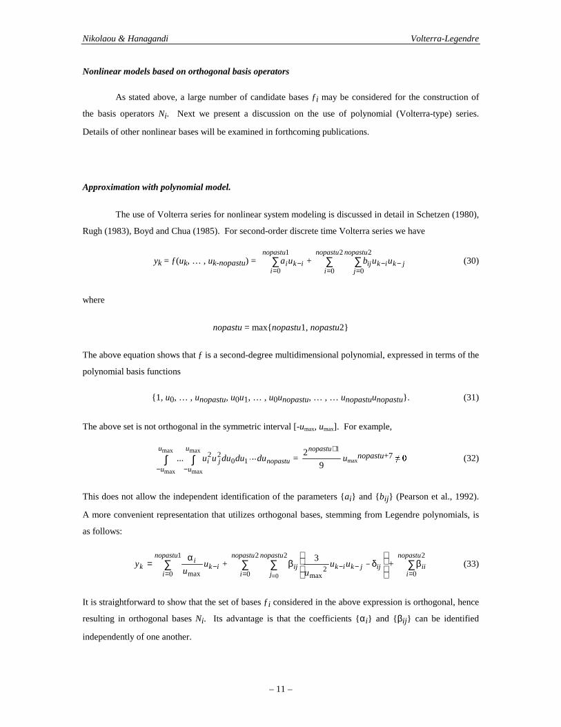
Nonlinear models based on orthogonal basis operators

As stated above, a large number of candidate bases ƒi may be considered for the construction of

the basis operators Ni. Next we present a discussion on the use of polynomial (Volterra-type) series.

Details of other nonlinear bases will be examined in forthcoming publications.

Approximation with polynomial model.

The use of Volterra series for nonlinear system modeling is discussed in detail in Schetzen (1980),

Rugh (1983), Boyd and Chua (1985). For second-order discrete time Volterra series we have

yk = ƒ(uk, … , uk-nopastu) = ∑=

−1

0

nopastu

iikiua + ∑ ∑

= =−−

2

0

2

0

nopastu

i

nopastu

jjkikij uub (30)

where

nopastu = max{ nopastu1, nopastu2}

The above equation shows that ƒ is a second-degree multidimensional polynomial, expressed in terms of the

polynomial basis functions

{ 1, u0, … , unopastu, u0u1, … , u0unopastu, … , … unopastuunopastu} . (31)

The above set is not orthogonal in the symmetric interval [-umax, umax]. For example,

∫ ∫− −

max

max

max

max

1022...

u

u

u

unopastuji dududuuu 6 =

9

2 1+nopastuumax

nopastu+7 7�8 (32)

This does not allow the independent identification of the parameters { ai} and { bij} (Pearson et al., 1992).

A more convenient representation that utilizes orthogonal bases, stemming from Legendre polynomials, is

as follows:

∑=

−α

=1

0 max

nopastu

iik

ik u

uy + ∑ ∑

=−−−

=

δβ

2

0

2

2max0

3nopastu

i

nopastu

jijjkikij uu

u+ ∑

=β

2

0

nopastu

iii (33)

It is straightforward to show that the set of bases ƒi considered in the above expression is orthogonal, hence

resulting in orthogonal bases Ni. Its advantage is that the coefficients { αi} and { βij} can be identified

independently of one another.


– 12 –

Remark 9: The above comment about the kernels being identifiable independently of one another

can be extended to kernels of higher order. The importance of this fact is that in nonlinear system

identification with orthogonal polynomial models the order of the polynomial (Volterra-Legendre)

approximation and the number of past inputs included in the model can be increased in a sequential manner,

without having to recalculate optimal values for the model coefficients. Thus, different numbers of past

inputs (nopastu1, nopastu2) may be successively considered for the first- and second-order terms. In

addition, terms of order 3, 4, … with small values for nopastu3, nopastu4, … may be successively

introduced. This greatly simplifies the identification procedure and provides significant insight into the

nature of the system modelled.

Approximation with multivariable harmonic model.

For basis functions ƒj selected as

ƒj(x0, x1, … , xnopastu)= exp[i ∑=

π nopastu

nnjn xk

u 0max]

(where i is the imaginary unit) orthogonality in the interval [-umax, umax] is straightforward to establish.

Sequential identification can then be carried out in a standard way, as explained above.

Model-predictive control with Volterra-Legendre models

To use a Volterra-Legendre model or an equivalent standard Volterra model for model-predictive

control, one can take at least two approaches:

Approach 1: Doyle et al. (1993) have shown how to use second-order Volterra models for the

design of unconstrained model-predictive controllers. Their technique relies on the inversion of the

nonlinear Volterra model, provided the inverse is stable. Zafiriou (1993) has examined the stability of the

resulting closed loop.

Approach 2: A Volterra model can also be used in model-predictive control based on on-line

optimization, particularly for problems with constraints. For constrained MPC with nonlinear models, most

efforts have concentrated on numerical aspects of the on-line nonlinear optimization that MPC performs

(Biegler and Rawlings, 1991; Gattu and Zafiriou, 1992; Sistu et al., 1993). In a recent development,

Meadows and Rawlings (1993) use a state-space approach to derive stability conditions for constrained


– 13 –

nonlinear MPC systems without modeling uncertainty, and show that unexpected difficulties may lurk

behind seemingly well-behaved nonlinear systems. They demonstrate that through a nonlinear state-space

system with polynomial nonlinearity, for which only discontinuous state feedback can result in closed-loop

stability. Robust stability conditions for constrained MPC with Volterra models are developed in Genceli

and Nikolaou (1994).

Since the emphasis of this work is on modeling rather than controller design, we will not discuss

theoretical issues of either approach. We will use both approaches in the case studies that follow for

illustration purposes.

Case studies

We will consider four reactor systems. For these systems we will assess open and closed-loop

nonlinearities. In addition, we will show how Volterra-Legendre series can be developed for a system with

significant nonlinearities.

Case study 1

Henson and Seborg (1990) studied the control of a two-continuous-stirred-tank-reactor-in-series

system (2CSTR) modeled by the nonlinear differential equations

dt

dCA1 = )( 11

AAf CCV

q− – k0 CA1 exp

−

1RT

E

dt

dT1 = )( 11

TTV

qf − +

p

A

C

CkH

ρ∆− 10)(

exp

−

1RT

E+

1VC

C

p

pcc

ρρ

qc )(exp1 11 TTCq

hAcf

pccc−

ρ

−

dt

dCA2 = )( 212

AA CCV

q− – k0 CA2 exp

−

2RT

E

dt

dT2 = )( 212

TTV

q− +

p

A

C

CkH

ρ∆− 20)(

exp

−

2RT

E+

+ 2VC

C

p

pcc

ρρ

qc

ρ+

ρ− −− )(expexp1 1

121

2 TTCq

hATT

Cq

hAcf

pcccpccc.


– 14 –

An irreversible exothermic reaction,

BAk

→

occurs in the two reactors. Notation and numerical values are provided in Table 1. Approximation of the

derivatives in the model equations by forward finite differences (δτ = 0.1) defines the (discrete-time)

nonlinear operator

P2CSTR : [u1, u2, u3, . . . , unosteps]T → [y1, y2, . . . , ynosteps]

T

The linearization Ls of P2CSTR around the steady state (u, y) = (0, 0), is realized by linear difference

equations.

We apply our theory to examine the nonlinearity characteristics of the above system. The code

was written in FORTRAN 77. The subroutine RNUN from the IMSL (1989) library was used for random

number generation. All calculations were performed in a Sun SparcStation 1.

Application of equations (20) and (21) yielded the results of Figure 1. It can be seen that for

inputs u in the ranges [– 0.01, 0.01], [– 0.05, 0.05] and [–0.10, 0.10] the coefficients hi for the optimal

linear approximations Lopt,j are virtually identical to those of the linearization Ls of P2CSTR around its

steady state. This, however, does not suggest that the nonlinearity of the operator P2CSTR is negligible for

these ranges of inputs, as one might expect. This statement is supported by the results of Table 2, where the

2-norms of P2CSTR, Lopt,1, … , Lopt,4, and Ls in growing intervals [umin, umax] are shown to be increasingly

different. (Recall that |||||||| APAP −≥− .) Table 3 shows the nonlinearity magnitude of P2CSTR, and

provides additional evidence of the severe nonlinearity of this system. Figures 2 to 4 compare step

responses of the CSTR for inputs of magnitudes 0.01, 0.05, 0.10, to step responses of Ls and Lopt,j. There

is significant discrepancy between P2CSTR and Ls as well as between P2CSTR and Lopt,j, as predicted by

Tables 2 and 3. It should be mentioned that Henson and Seborg (1990) intuitively arrived at similar

qualitative conclusions, by considering step response simulations.

Given the high nonlinearity of this system, we attempted to model it with second-order Volterra-

Legendre series. The identification results are shown in Figures 5 to 8. In particular, as many first and

second order terms can be retained, as necessary. The retained nonzero terms will be optimal, and will not

have to be readjusted after the deletion of essentially zero terms, or after the possible addition of third

order terms. Comparison between Figures 2 to 4 (step responses of the actual system and its linear

approximations) and Figures 9 and 10 (step responses of the actual system and its second-order

Volterra-Legendre approximations) shows that second-order Volterra-Legendre series can produce a

significantly improved model of this system.


– 15 –

It should also be mentioned that no computational sophistication was used to accelerate the

Monte-Carlo simulations or smoothen the results. It is conjectured that more accurate results can be

obtained if these two actions are taken.

The next question that we pose for this reactor is “How are the nonlinearity characteristics of the

reactor altered if a linear feedback controller is used?” To design the controller, we use the standard linear

internal model control (IMC) methodology (Morari and Zafiriou, 1989), applied to the linear model Ls

(linearization of P2CSTR around the steady state)2. Several different values of α are used in the IMC filter

21)(

α−α−=

zzF

The results (for inputs in the interval [–0.05, 0.05]) are shown in Table 4 and Figs. 11 and 12. Small α

results in aggressive control action corresponding to large inputs u to the process. Such inputs drive the

process to high nonlinearity regimes. On the other hand, large α results in “small” control action u, that

makes the nonlinearity of the process less pronounced (Fig. 14). As Table 4 predicts, despite the fact that

the open-loop system is “strongly” nonlinear (as demonstrated by the results in Tables 2 and 3), the

closed-loop system is significantly less nonlinear. This is illustrated in Fig. 13, where closed-loop

responses of the process with linear feedback control are compared to the ideal linear response F(z) that

would result if the process were linear. The linearizing effects of feedback are clear. Such effects have

long been claimed (Black, 1934; 1977) but hardly ever quantified. For verification purposes, Figs. 15 to

18 show simulations for the rejection of an external disturbance (Tf).

Case study 2

Nikolaou and Hanagandi (1993) studied a non-isothermal continuous stirred tank reactor (CSTR)

modelled by the equations (Stephanopoulos, 1984)

dt

dCA = V

FI [CAI – CA] – k CA exp

−

RT

E

dt

dT=

V

FI [TI – T] – P

R

C

H

ρ∆

k CA exp

−

RT

E–

VC

Q

Pρ

2 It should be noted that Henson and Seborg (1990) compared their nonlinear (exact-linearization based(Isidori, 1989; Kravaris and Kantor, 1990)) controller to a linear PI controller. That is not an entirely faircomparison, since a PI is not the best linear controller that can be used for that process. In fact, as shownby the results of Table 7, a linear IMC controller may be comparable to a nonlinear controller, as verifiedby the simulations in Fig. 7. This makes clear the importance of being able to quantitatively characterizenonlinearities.


– 16 –

Parameter values are shown in Table 5. This reactor has an Arrhenius type of nonlinearity, which is usually

considered severe. As Tables 6 and 7 show, application of the 2-norm theory reveals that, on the average,

this is not the case for inputs in the intervals [-0.10, 0.10], [-0.40, 0.40] and [-0.50, 0.50]. Table 8 shows

the 2-norm for the closed-loop operator PCL when a linear IMC controller with a first-order filter α−α−

z

1 is

used. The set-point ySP varied in the range [ ±0.0547894] corresponding to a ±30 K change in temperature.

Table 8 shows the closed-loop nonlinearity. It remains low. Nonlinearity does become important for larger

inputs. In fact, there is a significant advantage in using nonlinear vs. linear control if the system if forced to

operate in the severe nonlinearity range, as shown by Nikolaou and Hanagandi (1993) who used a nonlinear

controller based on a recurrent neural network model.

Case study 3

We will briefly summarize our conclusions for this example, treated in detail in Nikolaou (1993a).

The reaction

CBAkk 21→→

occurs in an isothermal continuous stirred-tank reactor (ICSTR), modelled by the dimensionless equations

(Ray, 1981)

dt

dx= – x– Da1 x2 + 1 + u

dt

dz= Da1 x2 – z – Da2 z1/2

Notation and numerical values are provided in Table 9. Notice the natural lower bound on the input u.

Although the nonlinearity of this reactor is polynomial, hence “mild” , it becomes significant if large enough

inputs are considered (Tables 10 and 11). The important information provided by the 2-norm is how large

inputs must be considered before nonlinearity becomes significant (e.g. inputs in [–1, 5] or [–1, 10]) and

how significant it becomes.


– 17 –

A closed-loop with this reactor is also examined. The reactor nonlinearity is augmented by the

saturation nonlinearity acting on the input (Fig. 19). Figure 20 shows that for small set-point changes tight

control is more linearizing, while for larger set-point change ranges looser control is more linearizing, since

it activates the saturation nonlinearity less frequently.

Case study 4

Uppal et al. (1974) studied the following reactor (U-CSTR).

dt

dx1 = – x1 + Da(1 – x1)exp

γ+ 2

2

1x

x

dt

dx2 = – x2 + B Da(1 – x1)exp

γ+ 2

2

1x

x+ β(yc – x2) + d

y = x2

Parameter definitions and values are given in Table 12. This reactor exhibits interesting nonlinear behavior,

and has been studied extensively. Piovoso et al. (1993) studied the application of three nonlinear control

strategies for this system. Nonlinear controller synthesis via system identification by neural networks was

reported in Jones et al. (1994). Hernández and Arkun (1992) investigated the control related properties of a

back-propagation neural network model of this reactor. Limqueco and Kantor (1990) constructed a

nonlinear observer for the reactor model, after transforming it to a linear system with nonlinear output

injection, and designed a globally linearizing controller for this system. As reported by Limqueco and

Kantor (1990), a disturbance of –5 K in the feed temperature will produce drastic changes in the reactor

temperature (ignition/extinction behavior).

Here we apply the 2-norm theory to investigate the nonlinearity of this reactor. The results are

presented in Table 13. Comparison of the values in columns 3 and 4 in Table 13, shows that the system is

“ fairly” linear in the corresponding input ranges. This fact is supported by the linear variation of the system

“gain” max

||||

u

PUCSTR vs. umax as indicated in column 5. Fig. 21 shows the closed-loop performance of a linear

IMC controller designed on the basis of Lopt,2, for different set-point changes. At t=40.0 a disturbance of –

5 K in the feed temperature is introduced to demonstrate a large drift in temperature and at t=80.0 the linear

IMC controller is turned on to bring the temperature to the steady state of 1.1. Comparing the linear


– 18 –

controller performance with that of the nonlinear controller (reported in Limqueco and Kantor (1990))

again demonstrates that, for the set-point changes intended, linear control is still a good option.

Discussion and conclusions

The 2-norm introduced in our earlier work provides a framework for dealing with the problem of

quantifying nonlinearities for dynamic systems. In this work we presented some extensions of the original

theory, and examined its implications for modeling nonlinear systems with Volterra series. Our conclusion

is that nonlinearities can be usefully quantified by the 2-norm for various ranges of process inputs. A

nonlinear system may or may not necessitate the use of a nonlinear model, depending, of course, on the task

for which this model is developed. For some nonlinear systems a linear model may be a very good

approximation, provided inputs to the system remain within a certain range. In addition, even if a linear

model may be a poor approximation for a real system, a linear model may be effectively used in controller

design which can directly rival nonlinear controller design. Given the significant effort required to design

and maintain nonlinear controllers (Bequette, 1991) a quantitative analysis of the need for such an approach

would be a worthwhile task to complete before nonlinear control is attempted. For the specific case of

modeling with Volterra series we showed how the proposed theory can be used to construct orthogonal

Volterra series (based on Legendre polynomials) which greatly simplify the modeling process through

sequential identification of Volterra kernels of various orders, independently of one another. Four case

studies were presented to illustrate the above issues.

The theory presented in this paper has the potential for several extensions and applications. An

extended list is presented in Nikolaou (1993a).


– 19 –

Nomenclature

A operator (either linear or nonlinear): ℜ nosteps → ℜ nosteps

α parameter of the linear filter 21

)(

α−α−=

zzF

Γi linear operator ℜ nosteps → ℜ nosteps, used as orthonormal basis in the representation of L

gi, ai coefficients used in the representation of the nonlinear operators N, Nopt in terms of Ni

hi coefficients used in the representation of a linear operator in terms of Li

I the identity operator

L linear operator: ℜ nosteps → ℜ nosteps

Li linear operator ℜ nosteps → ℜ nosteps, used as basis in the representation of L

Lopt,j Optimal linear approximation of a nonlinear operator in the interval No. j

lp the space of sequence with finite p-norm

N nonlinear operator: ℜ nosteps → ℜ nosteps

Ni basis nonlinear operator ℜ nosteps → ℜ nosteps, used in the representation of N

nobases the number of basis operators used for the representation of a nonlinear operator

noinputs the number of input sequences considered in the calculation of the inner product of twooperators

nopastu the number of past values of the input u considered in a moving-average type of model

nosteps the number of time-steps considered in the calculation of the inner product of two operators

O the null operator: ℜ nosteps → ℜ nosteps

P nonlinear operator: ℜ nosteps → ℜ nosteps

Q nonlinear operator: ℜ nosteps → ℜ nosteps

0 the zero vector in ℜ nosteps

ℜ the set of real numbers

ℜ n the set of n-dimensional real vectors

σ standard deviation

s steady state


– 20 –

u input sequence to a nonlinear system, =̂ [u1, u2, . . . , unosteps]T

umax upper bound for the entries of the input vector u

umin lower bound for the entries of the input vector u

y output sequence of a nonlinear system, =̂ [y1, y2, . . . , ynosteps]T

SPymax upper bound of ySP

ySP set-point of y

|| . || the 2-norm of an operator

|| . ||ip the induced p-norm of an operator

|| . ||p the p-norm of a vector in ℜ n, defined as pn

i

piu

/1

1||

∑=

if 1 9 p < :�; ||max,,1

ini

u<=, if ∞=p

f nonlinear function: ℜ nosteps → ℜ

ƒi nonlinear function: ℜ nosteps → ℜ , used as a basis in the representation of ƒ

QP; inner product of the operators P, Q

yx, inner product of the vectors x, y

Acronyms

ARMA Auto regressive moving average

CL CSTR closed loop

CSTR Continuous stirred tank reactor

ICL ICSTR closed loop

ICSTR Isothermal CSTR

MA Moving average

MARS Multivariate adaptive regression splines

UCSTR CSTR studied by Uppal et al. (1974)

2CSTR System of two CSTRs studied by Henson and Seborg (1990)


– 21 –

Literature cited

Bakshi, B. R., and G. Stephanopoulos, “Wave-net: a Multiresolution, Hierarchical Neural Network withLocalized Learning” , AIChE J., 39, 1, 57-81 (1993).

Bequette, B. W., “Nonlinear Control of Chemical Processes: A Review” , Ind. Eng. Chem. Res., 30,1391-1413 (1991).

Black, H. S., “ Inventing the negative feedback amplifier” , IEEE Spectrum., 55-60, (Dec. 1977).

Black, H. S., “Stabilized feedback amplifiers” , Bell Syst. Tech. J., 1-18, (Jan. 1934).

Boyd, S., and L. Chua, “Fading Memory and the Problem of Approximating Nonlinear Operators withVolterra Series” , IEEE Trans. Cir. Sys., vol. CAS-32, No. 11, 1150-1161 (1985).

Buckley, P. S., Second Eng. Found. Conf. on Chem. Proc. Contr., Sea Island, GA, Jan. (1981).

Desoer, C. A., and M. Vidyasagar, Feedback Systems: Input-Output Properties, Academic Press, NewYork (1975).

Desoer, C. A., and Y.-T. Wang, “Foundations of Feedback Theory for Nonlinear Dynamical Systems” ,IEEE Trans. Circ. Syst., vol. CAS-27, no. 2, 104-123 (1980).

Doyle, F. J., B. A. Ogunnaike, and R. K. Pearson, “Nonlinear Model Predictive Control Using SecondOrder Volterra Models” , AIChE Annual Meeting, Miami Beach (1992).

Doyle, F., and F. Allgöwer, “Nonlinear Process Control - Which way to the promised land?” , CPC Vpreprints, Tahoe City, CA (1996).

Edgar, T. F., “Current Problems in Process Control” , IEEE Control Systems magazine, 13-15 (1989).

Fleming, W. H.. (Chair), SIAM Report of the Panel on Future Directions in Control Theory: AMathematical Perspective, SIAM Publication (1988).

Foss, A. S., “Critique of Chemical Process Control Theory” , AIChE J. vol. 199, 209-215 (1973).

Friedman, J. H., “Multivariate Adaptive Regression Splines” , The Annals of Statistics, 19, No. 1, 1-141(1991).

García, C. E., and D. M. Prett, “Design Methodology based on the Fundamental Control ProblemFormulation” , Shell Process Control Workshop, Houston, TX (1986).

Genceli, H., and M. Nikolaou, “Design of Robust Constrained Model Predictive Controllers with VolterraSeries” , AIChE J., to appear (1995).

Henson, M. A., and D. E. Seborg, “ Input-Output Linearization of General Nonlinear Processes” , AIChE J.,36, 11, 1753-1757 (1990).

Hopfield, J. J., “Neural Networks and Physical Systems with Emergent Computational Abilities” , Proc.Natl. Acad. Sci. USA, 79, 2554 (1982).

IMSL, User’s Manual-IMSL Math/Library, Version 1.1, Houston (1989).


– 22 –

Isidori, A., Nonlinear Control Systems: An Introduction, 2nd Ed., Springer-Verlag, (1989).

Kane, L., “How combined technologies aid model-based control” , IN CONTROL, vol VI, No. 3, 6-7 (1993).

Kolmogorov, A. N., and S. V. Fomin, Introductory Real Analysis, Dover, New York (1970).

Kravaris, C., and J. C. Kantor, “Geometric Methods for Nonlinear Process Control. 1. Background” , Ind.Eng. Chem. Res., 29, 2295-2310 (1990).

Kravaris, C., and J. C. Kantor, “Geometric Methods for Nonlinear Process Control. 2. ControllerSynthesis” , Ind. Eng. Chem. Res., 29, 2310-2323 (1990).

Kumar, A., and Daoutidis, P., “Feedback Regularization And Control Of Nonlinear Differential-Algebraic-Equation Systems” , AIChE Journal, 42, 8, 2175-2198 (1996).

Longwell, E. J., “Chemical Processes and Nonlinear Control Technology” , Proceedings of CPC IV,445-476 (1991)

Luenberger, D. G., Optimization by Vector Space Methods, John Wiley and Sons (1969).

Manousiouthakis, V., and D. Sourlas, “Development of Linear Models for Nonlinear Systems” , paper 125c,AIChE Annual Meeting, Miami, FL (1992).

Mayne, D. Q., “Nonlinear Model Predictive Control: An Assessment” , CPC V preprints, Tahoe City, CA(1996).

Morari, M. and E. Zafiriou, Robust Process Control, Prentice Hall (1989).

Morari, M., “Three Critiques of Process Control revisited a Decade Later” , Shell Process ControlWorkshop, Houston, TX (1986).

National Research Council Committee, Frontiers in Chemical Engineering: Research Needs andOpportunities, National Academy Press (1988).

Nijmeijer, H., and A. J. van der Schaft, Nonlinear Dynamical Control Systems, Springer-Verlag (1990).

Nikolaou, M. and V. Manousiouthakis, “A Hybrid Approach to Nonlinear System Stability andPerformance” , AIChE Journal, 35, 4, 559-572 (1989).

Nikolaou, M., “Neural Network Modeling of Nonlinear Dynamical Systems” , ACC Proceedings,1460-1464, San Francisco (1993).

Nikolaou, M., “When is Nonlinear Dynamic Modeling Necessary?” , ACC Proceedings, 910-914, SanFrancisco (1993).

Nikolaou, M., and V. Hanagandi, “ Input-Output Exact Linearization of Nonlinear Dynamical SystemsModeled by Recurrent Neural Networks” , AIChE J., 39, 11, 1890-1894 (1993).

Nikolaou, M., and V. Hanagandi, “Recurrent Neural Networks in Decoupling Control of MultivariableNonlinear Systems” , submitted to Chem. Eng. Communications, (1993).

Ogunnaike, B., and R. Wright, “ Industrial Applications of Nonlinear Control” , CPC V preprints, TahoeCity, CA (1996).


– 23 –

Pearson, R. K., B. A. Ogunnaike, and F. J. Doyle, “ Identification of Discrete Convolution Models forNonlinear Processes” , paper 125b, AIChE Annual Meeting, Miami Beach (1992).

Prett, D. M., and C. E. García, Fundamental Process Control, Butterworths, Stoneham, MA (1988).

Rawlings, J. B., E. S. Meadows, and K. R. Muske, “Nonlinear Model Predictive Control: A Tutorial andSurvey” , to be presented at ADCHEM ’94, Kyoto, Japan (1994).

Ray, W. H., Advanced Process Control, McGraw-Hill (1981).

Rugh, W. J., Nonlinear System Theory, Johns Hopkins Press (1983).

Rumelhart, D. E., G. E. Hinton, and R. J. Williams, “Learning Representations by Back-propagatingErrors” , Nature, 323, 533 (1986).

Schetzen, M., The Volterra and Wiener Theories of Nonlinear Systems, John Wiley and Sons (1980).

Soroush, .M., and Kravaris, C., “Discrete-Time Nonlinear Feedback Control Of Multivariable Processes” ,AIChE Journal, 42, 1, 187-203 (1996).

Theiler, J., S. Eubank, A. Longtin, B. Galdrikian, and J. D. Farmer, “Testing for nonlinearity in time series:the method of surrogate data” , Physica D, 58, 77-94 (1992).

Tong, H., Non-linear Time Series: A Dynamical System Approach, Clarendon Press, Oxford (1990).

Tsay, R. S., “Nonlinear time series analysis: diagnostics and modelling” , Statistical Sinica, 1, 431-451(1991).

Yosida, K., Functional Analysis, Springer Verlag (1974).

Zafiriou, E., “Stability of Model Predictive Control with Volterra Series” , AIChE Annual Meeting, St. Louis(1993).


– 24 –

Table 1. Parameters of 2CSTR (Henson and Seborg, 1990)

VARIABLE DEFINITION VALUE

CA1, CA2 Concentrations of species A in CSTRs 1 and 2 state variables

T1, T2 Temperatures of CSTRs 1 and 2 state variables

CAf Feed concentration of species A 1 mol/L

Tf Feed temperature 350 K

Tcf Coolant feed temperature 350 K

q Feed flowrate 100 L/min

E/R Activation energy 1 × 104 K

V1 = V2 Volumes of CSTRs 1 and 2 100 L

k0 Reaction rate constant 7.2 × 1010 min–1

u = cs

csc

q

qq − ; dimensionless coolant flowrate input variable; =�>@?

ysA

sAA

C

CC

1

11 −= ; dimensionless reactant concentration output

– A H Heat of reaction 4.78 × 1010 j/mol

h A1 = h A2 (Heat transfer coefficient) × (Area) 1.67 × 105 j/min/K

Cp = Cpc Specific heat 0.239 j/g/K

ρ = ρc density 1000 g/L

CA1s Steady state concentration of species A in CSTR 1 0.088228 mol/L

CA2s Steady state concentration of species A in CSTR 2 0.0052926 mol/L

T1s Steady state temperature of CSTR 1 441.2193 K

T2s Steady state temperature of CSTR 2 449.5177 K

qcs Steady state coolant flowrate 100 l/min


– 25 –

Table 2. Norms of P2CSTR, its steady-state linearization Ls, and optimal linear approximations Lopt,j

over various input intervals [umin, umax]

j umax,j =

–umin,j

||P2CSTR||2 ||Ls||2 ||Lopt,1||2 ||Lopt,2||2 ||Lopt,3||2 ||Lopt,4||22

max

22 ||||

u

P CSTR

1 0.01 4.30 10–9 4.56 10–9 4.57 10–9 4.62 10–9 4.80 10–9 6.00 10–9 4.30 10–9

2 0.05 1.09 10–7 1.14 10–7 1.14 10–7 1.16 10–7 1.20 10–7 1.50 10–7 4.37 10–9

3 0.10 4.61 10–7 4.56 10–7 4.57 10–7 4.63 10–7 4.80 10–7 6.00 10–7 4.61 10–9

4 0.20 2.43 10–6 1.83 10–6 1.83 10–6 1.85 10–6 1.92 10–6 2.40 10–6 6.07 10–9


– 26 –

Table 3. Error made in the approximation of P2CSTR by linear operators over various input

intervals [umin, umax] (entries in bold/italics refer to nonlinearity magnitude)j

||||

||||

2

2

CSTR

CSTRs

P

PL −

||||

||||

2

21,

CSTR

CSTRopt

P

PL −

||||

||||

2

22,

CSTR

CSTRopt

P

PL −

||||

||||

2

23,

CSTR

CSTRopt

P

PL −

||||

||||

2

24,

CSTR

CSTRopt

P

PL −

1 0.34 0.34 0.34 0.33 0.36

2 0.37 0.37 0.36 0.36 0.38

3 0.46 0.44 0.44 0.43 0.44

4 0.77 0.77 0.76 0.75 0.72


– 27 –

Table 4. Assessment of closed-loop nonlinearity for 2CSTR

α ||PCL||2 ||Lopt ||2||||

||||

CL

CLopt

P

PL −

0.4 2.73 10–7 3.26 10–7 0.19

0.5 2.15 10–7 2.14 10–7 0.097

0.6 1.60 10–7 1.61 10–7 0.090

0.7 1.14 10–7 1.14 10–7 0.078

0.9 3.24 10–8 3.33 10–7 0.059


– 28 –

Table 5. Parameters for CSTR (Nikolaou and Hanagandi, 1993)


CA Concentration of species A state variable

T Temperature of the reactor contents state variable

u Dimensionless heat removal rate (= s

s

Q

QQ −) input

y B�C D@E FHG C I FHJ E G GLK E D�MNE O P K QNO E�R =s

s

T

TT −) output

FI Inlet flowrate 1.133 m3/hr

V Reactor volume 1.36 m3

CAI Inlet concentration of species A 8008.00 mol/m3

k Reaction constant 1.08 × 107 1/hr

E/R Activation energy 8375.00 S TUHV

R Heat of reaction –69775.0 j/mol

TI Inlet feed temperature 373.3 W Xρ Density of reactor contents 800.80 kg/m3

Cp Specific heat 3140.00 J/(kg Y Z�[CAs Steady state concentration of species A 393.300 mol/l

Ts Steady state temperature 547.556 \ ]Qs Steady state heat removal rate 1.066 × 108


– 29 –

Table 6. Norms of PCSTR, its steady-state linearization Ls, and optimal linear approximations Lopt,j

over various input intervals [umin, umax]

j [uminj, umaxj] ||PICSTR||2 ||Ls||2 ||Lopt,1||2 ||Lopt,2||2 ||Lopt,3||2

max

||||

u

PCSTR

1 [-0.1, 0.1] 0.367 0.367 0.363 0.365 0.366 6.05

2 [-0.4, 0.4] 5.89 5.87 5.81 5.84 5.85 6.06

3 [-0.5, 0.5] 9.22 9.17 9.09 9.12 9.14 6.07


– 30 –

Table 7. Error made in the approximation of PCSTR by linear operators over various input intervals[umin, umax] (entries in bold/italics refer to nonlinearity magnitude)

j [uminj, umaxj]||||

||||

CSTR

CSTRs

P

PL −

||||

|||| 1,

CSTR

CSTRopt

P

PL −

||||

|||| 2,

CSTR

CSTRopt

P

PL −

||||

|||| 3,

CSTR

CSTRopt

P

PL −

1 [-0.1, 0.1] 0.0167 0.0174 0.0170 0.0169

2 [-0.4, 0.4] 0.0231 0.0241 0.0237 0.0236

3 [-0.5, 0.5] 0.0291 0.0301 0.0297 0.0295


– 31 –

Table 8. Assessment of closed-loop nonlinearity for CSTR

α ||PCL||2 ||Lopt||2||||

||||

CL

CLopt

P

PL −

0.00 268 268 0.0515

0.50 100 101 0.0463

0.80 35.0 34.9 0.0365

0.90 16.6 16.5 0.0301

0.95 7.91 7.90 0.00635


– 32 –

Table 9. Parameters of ICSTR


CA, CB Concentrations of species A and B in the ICSTR

CAf, CBf Concentrations of species A and B in the feed

CAref Reference concentration of species A

F Feed/effluent flowrate

V Reaction volume

k1, k2 Reaction rate constants

u system input; (= Aref

Af

C

C) ^�_@` a b

x, z system states (=

Aref

B

Aref

A

C

C

C

C, )

y Output (= (z - zs))

τ dimensionless time (= V

tF)

Da1, Da2Damköhler numbers (=

2/1

21,

Aref

Aref

FC

Vk

F

VCk)

(1.0, 2.0)

us Steady state value of the input u 0.0

xs, zs Steady state values of the states x, z (0.61803399,

0.030825002)


– 33 –

Table 10. Norms of PICSTR, its steady-state linearization Ls, and optimal linear approximations

Lopt,j over various input intervals [umin, umax]

j [uminj, umaxj] ||PICSTR||2 ||Ls||2 ||Lopt,1||2 ||Lopt,2||2 ||Lopt,3||2 ||Lopt,4||2

1 [– 0.1, 0.1] 2.35 10–6 2.33 10–6 2.33 10–6 2.30 10–6 1.48 10–5 2.74 10–5

2 [– 1, 1] 2.35 10–4 2.33 10–4 2.33 10–4 2.30 10–4 1.48 10–3 2.74 10–3

3 [– 1, 5] 0.163 2.67 10–2 2.67 10–2 2.67 10–2 0.166 0.334

4 [– 1, 10] 1.68 0.132 0.132 0.132 0.820 1.65


– 34 –

Table 11. Error made in the approximation of PICSTR by linear operators Lopt,j over various input

intervals [umin, umax] (entries in bold/italics refer to nonlinearity magnitude)

j||||

||||

ICSTR

ICSTRs

P

PL −

||||

|||| 1,

ICSTR

ICSTRopt

P

PL −

||||

|||| 2,

ICSTR

ICSTRopt

P

PL −

||||

|||| 3,

ICSTR

ICSTRopt

P

PL −

||||

|||| 4,

ICSTR

ICSTRopt

P

PL −

3 0.60 0.60 0.60 0.16 0.48

4 0.72 0.72 0.72 0.31 0.13


– 35 –

Table 12. Parameter values for UCSTR (Uppal et al., 1974)


x1 Dimensionless concentration of species A state variable

x2 Dimensionless temperature state variable

γ Dimensionless activation energy 20.0

β Dimensionless heat transfer coefficient 0.3

B Dimensionless adiabatic temperature rise 8.0

Da Damköhler number 0.072

yc Dimensionless cooling jacket temperature manipulated input

y = x2 controlled output

d Dimensionless feed temperature (disturbance) 0.0 (nominal value)

x1s Steady state values of the state x1 0.1539693

x2s Steady state values of the state x2 0.8859648

ycs Steady state value of the input 0.0


– 36 –

Table 13. Nonlinearity characteristics of PUCSTR over various input intervals [umin, umax]

(entries in bold/italics refer to nonlinearity magnitude)

j [uminj, umaxj] ||PUCSTR||2 ||Lopt||2

max

||||

u

PUCSTR

||||

|||| 2,

UCSTR

optUCSTR

P

LP −

1 [–1.0, 1.0] 4.18 10–3 4.24 10–3 0.0647 0.061

2 [–2.0, 2.0] 1.74 10–2 1.69 10–2 0.0329 0.12

3 [–2.5, 2.5] 2.81 10–2 2.65 10–2 0.0268 0.16

nonlinearity quantification and its application to

Documents