nonparametric statistics with applications in science...
TRANSCRIPT

Nonparametric Statistics with
Applications in Science and Engineering


Nonparametric Statistics with
Applications in Science and Engineering
Paul Kvam and Brani Vidakovic
A Wiley-Interscience Publication
JOHN WILEY & SONS, INC.
New York / Chichester / Weinheim / Brisbane / Singapore / Toronto


Contents
Preface xi
1 Introduction 11.1 Efficiency of Nonparametric Methods 31.2 Overconfidence Bias 51.3 Computing with MATLAB 51.4 Exercises 7References 7
2 Probability Basics 92.1 Helpful Functions 92.2 Events, Probabilities and Random Variables 112.3 Numerical Characteristics of Random Variables 122.4 Discrete Distributions 142.5 Continuous Distributions 172.6 Mixture Distributions 232.7 Exponential Family of Distributions 252.8 Stochastic Inequalities 262.9 Convergence of Random Variables 28
v

vi CONTENTS
2.10 Exercises 31References 32
3 Statistics Basics 333.1 Estimation 333.2 Empirical Distribution Function 343.3 Statistical Tests 363.4 Exercises 45References 46
4 Bayesian Statistics 474.1 The Bayesian Paradigm 474.2 Ingredients for Bayesian Inference 484.3 Bayesian Computation and Use of WinBUGS 614.4 Exercises 63References 67
5 Order Statistics 695.1 Joint Distributions of Order Statistics 705.2 Sample Quantiles 725.3 Tolerance Intervals 735.4 Asymptotic Distributions of Order Statistics 755.5 Extreme Value Theory 765.6 Ranked Set Sampling 765.7 Exercises 77References 80
6 Goodness of Fit 816.1 Kolmogorov-Smirnov Test Statistic 826.2 Smirnov Test to Compare Two Distributions 866.3 Specialized Tests 896.4 Probability Plotting 976.5 Runs Test 1006.6 Meta Analysis 1066.7 Exercises 109

CONTENTS vii
References 113
7 Rank Tests 1157.1 Properties of Ranks 1177.2 Sign Test 1187.3 Spearman Coefficient of Rank Correlation 1227.4 Wilcoxon Signed Rank Test 1267.5 Wilcoxon (Two-Sample) Sum Rank Test 1297.6 Mann-Whitney U Test 1317.7 Test of Variances 1337.8 Exercises 135References 139
8 Designed Experiments 1418.1 Kruskal-Wallis Test 1418.2 Friedman Test 1458.3 Variance Test for Several Populations 1488.4 Exercises 149References 152
9 Categorical Data 1539.1 Chi-Square and Goodness-of-Fit 1559.2 Contingency Tables 1599.3 Fisher Exact Test 1639.4 MCNemar Test 1649.5 Cochran’s Test 1679.6 Mantel-Haenszel Test 1679.7 CLT for Multinomial Probabilities 1719.8 Simpson’s Paradox 1729.9 Exercises 173References 180
10 Estimating Distribution Functions 18310.1 Introduction 18310.2 Nonparametric Maximum Likelihood 184

viii CONTENTS
10.3 Kaplan-Meier Estimator 18510.4 Confidence Interval for F 19210.5 Plug-in Principle 19310.6 Semi-Parametric Inference 19510.7 Empirical Processes 19710.8 Empirical Likelihood 19810.9 Exercises 201References 203
11 Density Estimation 20511.1 Histogram 20611.2 Kernel and Bandwidth 20711.3 Exercises 213References 215
12 Beyond Linear Regression 21712.1 Least Squares Regression 21812.2 Rank Regression 21912.3 Robust Regression 22112.4 Isotonic Regression 22712.5 Generalized Linear Models 23012.6 Exercises 237References 240
13 Curve Fitting Techniques 24113.1 Kernel Estimators 24313.2 Nearest Neighbor Methods 24713.3 Variance Estimation 24913.4 Splines 25113.5 Summary 25713.6 Exercises 258References 260
14 Wavelets 26314.1 Introduction to Wavelets 263

CONTENTS ix
14.2 How Do the Wavelets Work? 26614.3 Wavelet Shrinkage 27314.4 Exercises 281References 283
15 Bootstrap 28515.1 Bootstrap Sampling 28515.2 Nonparametric Bootstrap 28715.3 Bias Correction for Nonparametric Intervals 29215.4 The Jackknife 29515.5 Bayesian Bootstrap 29615.6 Permutation Tests 29815.7 More on the Bootstrap 30215.8 Exercises 302References 304
16 EM Algorithm 30716.1 Fisher’s Example 30916.2 Mixtures 31116.3 EM and Order Statistics 31516.4 MAP via EM 31716.5 Infection Pattern Estimation 31816.6 Exercises 319References 321
17 Statistical Learning 32317.1 Discriminant Analysis 32417.2 Linear Classification Models 32617.3 Nearest Neighbor Classification 32917.4 Neural Networks 33317.5 Binary Classification Trees 33817.6 Exercises 346References 346
18 Nonparametric Bayes 349

x CONTENTS
18.1 Dirichlet Processes 35018.2 Bayesian Categorical Models 35718.3 Infinitely Dimensional Problems 36018.4 Exercises 364References 366
A MATLAB 369A.1 Using MATLAB 369A.2 Matrix Operations 372A.3 Creating Functions in MATLAB 374A.4 Importing and Exporting Data 375A.5 Data Visualization 380A.6 Statistics 386
B WinBUGS 397B.1 Using WinBUGS 398B.2 Built-in Functions 401
MATLAB Index 405
Author Index 409
Subject Index 413

Preface
Danger lies not in what we don’t know, but in what we think we knowthat just ain’t so.
Mark Twain (1835 – 1910)
As Prefaces usually start, the author(s) explain why they wrote the bookin the first place – and we will follow this tradition. Both of us taught thegraduate course on nonparametric statistics at the School of Industrial andSystems Engineering at Georgia Tech (ISyE 6404) several times. The audi-ence was always versatile: PhD students in Engineering Statistics, ElectricalEngineering, Management, Logistics, Physics, to list a few. While comprisinga non homogeneous group, all of the students had solid mathematical, pro-gramming and statistical training needed to benefit from the course. Givensuch a nonstandard class, the text selection was all but easy.
There are plenty of excellent monographs/texts dealing with nonparamet-ric statistics, such as the encyclopedic book by Hollander and Wolfe, Non-parametric Statistical Methods, or the excellent evergreen book by Conover,Practical Nonparametric Statistics, for example. We used as a text the 3rdedition of Conover’s book, which is mainly concerned with what most of usthink of as traditional nonparametric statistics: proportions, ranks, categor-ical data, goodness of fit, and so on, with the understanding that the textwould be supplemented by the instructor’s handouts. Both of us ended upsupplying an increasing number of handouts every year, for units such as den-sity and function estimation, wavelets, Bayesian approaches to nonparametricproblems, the EM algorithm, splines, machine learning, and other arguably
xi
xii PREFACE
modern nonparametric topics. About a year ago, we decided to merge thehandouts and fill the gaps.
There are several novelties this book provides. We decided to intertwineinformal comments that might be amusing, but tried to have a good balance.One could easily get carried away and produce a preface similar to that ofcelebrated Barlow and Proschan’s, Statistical Theory of Reliability and LifeTesting: Probability Models, who acknowledge greedy spouses and obnoxiouschildren as an impetus to their book writing. In this spirit, we featured pho-tos and sometimes biographic details of statisticians who made fundamentalcontributions to the field of nonparametric statistics, such as Karl Pearson,Nathan Mantel, Brad Efron, and Baron Von Munchausen.
Computing. Another specificity is the choice of computing support. Thebook is integrated with MATLAB c© and for many procedures covered in thisbook, MATLAB’s m-files or their core parts are featured. The choice ofsoftware was natural: engineers, scientists, and increasingly statisticians arecommunicating in the “MATLAB language.” This language is, for example,taught at Georgia Tech in a core computing course that every freshman engi-neering student takes, and almost everybody around us “speaks MATLAB.”The book’s website:
http://www2.isye.gatech.edu/NPbook
contains most of the m-files and programming supplements easy to trace anddownload. For Bayesian calculation we used WinBUGS, a free software fromCambridge’s Biostatistics Research Unit. Both MATLAB and WinBUGS arebriefly covered in two appendices for readers less familiar with them.
Outline of Chapters. For a typical graduate student to cover the fullbreadth of this textbook, two semesters would be required. For a one-semestercourse, the instructor should necessarily cover Chapters 1–3, 5–9 to start.Depending on the scope of the class, the last part of the course can includedifferent chapter selections.
Chapters 2–4 contain important background material the student needs tounderstand in order to effectively learn and apply the methods taught in anonparametric analysis course. Because the ranks of observations have specialimportance in a nonparametric analysis, Chapter 5 presents basic results fororder statistics and includes statistical methods to create tolerance intervals.
Traditional topics in estimation and testing are presented in Chapters 7–10 and should receive emphasis even to students who are most curious aboutadvanced topics such as density estimation (Chapter 11), curve-fitting (Chap-ter 13) and wavelets (Chapter 14). These topics include a core of rank teststhat are analogous to common parametric procedures (e.g., t-tests, analysisof variance).
Basic methods of categorical data analysis are contained in Chapter 9. Al-

PREFACE xiii
though most students in the biological sciences are exposed to a wide varietyof statistical methods for categorical data, engineering students and other stu-dents in the physical sciences typically receive less schooling in this quintessen-tial branch of statistics. Topics include methods based on tabled data, chi-square tests and the introduction of general linear models. Also included inthe first part of the book is the topic of “goodness of fit” (Chapter 6), whichrefers to testing data not in terms of some unknown parameters, but the un-known distribution that generated it. In a way, goodness of fit represents aninterface between distribution-free methods and traditional parametric meth-ods of inference, and both analytical and graphical procedures are presented.Chapter 10 presents the nonparametric alternative to maximum likelihoodestimation and likelihood ratio based confidence intervals.
The term “regression” is familiar from your previous course that introducedyou to statistical methods. Nonparametric regression provides an alternativemethod of analysis that requires fewer assumptions of the response variable. InChapter 12 we use the regression platform to introduce other important topicsthat build on linear regression, including isotonic (constrained) regression,robust regression and generalized linear models. In Chapter 13, we introducemore general curve fitting methods. Regression models based on wavelets(Chapter 14) are presented in a separate chapter.
In the latter part of the book, emphasis is placed on nonparametric proce-dures that are becoming more relevant to engineering researchers and prac-titioners. Beyond the conspicuous rank tests, this text includes many ofthe newest nonparametric tools available to experimenters for data analysis.Chapter 17 introduces fundamental topics of statistical learning as a basisfor data mining and pattern recognition, and includes discriminant analysis,nearest-neighbor classifiers, neural networks and binary classification trees.Computational tools needed for nonparametric analysis include bootstrap re-sampling (Chapter 15) and the EM Algorithm (Chapter 16). Bootstrap meth-ods, in particular, have become indispensable for uncertainty analysis withlarge data sets and elaborate stochastic models.
The textbook also unabashedly includes a review of Bayesian statistics andan overview of nonparametric Bayesian estimation. If you are familiar withBayesian methods, you might wonder what role they play in nonparametricstatistics. Admittedly, the connection is not obvious, but in fact nonpara-metric Bayesian methods (Chapter 18) represent an important set of tools forcomplicated problems in statistical modeling and learning, where many of themodels are nonparametric in nature.
The book is intended both as a reference text and a text for a graduatecourse. We hope the reader will find this book useful. All comments, sugges-tions, updates, and critiques will be appreciated.

xiv PREFACE
Acknowledgments. Before anyone else we would like to thank our wives,Lori Kvam and Draga Vidakovic, and our families. Reasons they toleratedour disorderly conduct during the writing of this book are beyond us, but welove them for it.
We are especially grateful to Bin Shi, who supported our use of MATLABand wrote helpful coding and text for the Appendix A. We are grateful toMathWorks Statistics team, especially to Tom Lane who suggested numerousimprovements and updates in that appendix. Several individuals have helpedto improve on the primitive drafts of this book, including Saroch Boonsiripant,Lulu Kang, Hee Young Kim, Jongphil Kim, Seoung Bum Kim, Kichun Lee,and Andrew Smith.
Finally, we thank Wiley’s team, Melissa Yanuzzi, Jacqueline Palmieri andSteve Quigley, for their kind assistance.
Paul H. KvamSchool of Industrial and System Engineering
Georgia Institute of Technology
Brani VidakovicSchool of Biomedical Engineering
Georgia Institute of Technology

1Introduction
For every complex question, there is a simple answer.... and it is wrong.
H. L. Mencken
Jacob Wolfowitz (Figure 1.1a) first coined the term nonparametric, saying“We shall refer to this situation [where a distribution is completely determinedby the knowledge of its finite parameter set] as the parametric case, and denotethe opposite case, where the functional forms of the distributions are unknown,as the non-parametric case” (Wolfowitz, 1942). From that point on, nonpara-metric statistics was defined by what it is not: traditional statistics basedon known distributions with unknown parameters. Randles, Hettmansperger,and Casella (2004) extended this notion by stating “nonparametric statisticscan and should be broadly defined to include all methodology that does notuse a model based on a single parametric family.”
Traditional statistical methods are based on parametric assumptions; thatis, that the data can be assumed to be generated by some well-known family ofdistributions, such as normal, exponential, Poisson, and so on. Each of thesedistributions has one or more parameters (e.g., the normal distribution hasµ and σ2), at least one of which is presumed unknown and must be inferred.The emphasis on the normal distribution in linear model theory is often jus-tified by the central limit theorem, which guarantees approximate normalityof sample means provided the sample sizes are large enough. Other distribu-tions also play an important role in science and engineering. Physical failuremechanisms often characterize the lifetime distribution of industrial compo-
1

2 INTRODUCTION
(a) (b)
Fig. 1.1 (a) Jacob Wolfowitz (1910–1981) and (b) Wassily Hoeffding (1914–1991),pioneers in nonparametric statistics.
nents (e.g., Weibull or lognormal), so parametric methods are important inreliability engineering.
However, with complex experiments and messy sampling plans, the gener-ated data might not be attributed to any well-known distribution. Analystslimited to basic statistical methods can be trapped into making parametricassumptions about the data that are not apparent in the experiment or thedata. In the case where the experimenter is not sure about the underlying dis-tribution of the data, statistical techniques are needed which can be appliedregardless of the true distribution of the data. These techniques are callednonparametric methods, or distribution-free methods.
The terms nonparametric and distribution-free are not synonymous...Popular usage, however, has equated the terms ... Roughly speaking, anonparametric test is one which makes no hypothesis about the value ofa parameter in a statistical density function, whereas a distribution-freetest is one which makes no assumptions about the precise form of thesampled population.
J. V. Bradley (1968)
It can be confusing to understand what is implied by the word “nonpara-metric”. What is termed modern nonparametrics includes statistical modelsthat are quite refined, except the distribution for error is left unspecified.Wasserman’s recent book All Things Nonparametric (Wasserman, 2005) em-phasizes only modern topics in nonparametric statistics, such as curve fitting,density estimation, and wavelets. Conover’s Practical Nonparametric Statis-tics (Conover, 1999), on the other hand, is a classic nonparametrics textbook,but mostly limited to traditional binomial and rank tests, contingency tables,and tests for goodness of fit. Topics that are not really under the distribution-free umbrella, such as robust analysis, Bayesian analysis, and statistical learn-ing also have important connections to nonparametric statistics, and are all

EFFICIENCY OF NONPARAMETRIC METHODS 3
featured in this book. Perhaps this text could have been titled A Bit Lessof Parametric Statistics with Applications in Science and Engineering, butit surely would have sold fewer copies. On the other hand, if sales werethe primary objective, we would have titled this Nonparametric Statistics forDummies or maybe Nonparametric Statistics with Pictures of Naked People.
1.1 EFFICIENCY OF NONPARAMETRIC METHODS
It would be a mistake to think that nonparametric procedures are simplerthan their parametric counterparts. On the contrary, a primary criticism ofusing parametric methods in statistical analysis is that they oversimplify thepopulation or process we are observing. Indeed, parametric families are notmore useful because they are perfectly appropriate, rather because they areperfectly convenient.
Nonparametric methods are inherently less powerful than parametric meth-ods. This must be true because the parametric methods are assuming moreinformation to construct inferences about the data. In these cases the esti-mators are inefficient, where the efficiencies of two estimators are assessed bycomparing their variances for the same sample size. This inefficiency of onemethod relative to another is measured in power in hypothesis testing, forexample.
However, even when the parametric assumptions hold perfectly true, wewill see that nonparametric methods are only slightly less powerful than themore presumptuous statistical methods. Furthermore, if the parametric as-sumptions about the data fail to hold, only the nonparametric method isvalid. A t-test between the means of two normal populations can be danger-ously misleading if the underlying data are not actually normally distributed.Some examples of the relative efficiency of nonparametric tests are listed inTable 1.1, where asymptotic relative efficiency (A.R.E.) is used to compareparametric procedures (2nd column) with their nonparametric counterparts(3rd column). Asymptotic relative efficiency describes the relative efficiencyof two estimators of a parameter as the sample size approaches infinity. TheA.R.E. is listed for the normal distribution, where parametric assumptionsare justified, and the double-exponential distribution. For example, if the un-derlying data are normally distributed, the t-test requires 955 observations inorder to have the same power of the Wilcoxon signed-rank test based on 1000observations.
Parametric assumptions allow us to extrapolate away from the data. Forexample, it is hardly uncommon for an experimenter to make inferences abouta population’s extreme upper percentile (say 99th percentile) with a sampleso small that none of the observations would be expected to exceed thatpercentile. If the assumptions are not justified, this is grossly unscientific.
Nonparametric methods are seldom used to extrapolate outside the range

4 INTRODUCTION
Table 1.1 Asymptotic relative efficiency (A.R.E.) of some nonparametric tests
Parametric Nonparametric A.R.E. A.R.E.Test Test (normal) (double exp.)
2-Sample Test t-test Mann-Whitney 0.955 1.503-Sample Test one-way layout Kruskal-Wallis 0.864 1.50Variances Test F -test Conover 0.760 1.08
of observed data. In a typical nonparametric analysis, little or nothing can besaid about the probability of obtaining future data beyond the largest sampledobservation or less than the smallest one. For this reason, the actual measure-ments of a sample item means less compared to its rank within the sample.In fact, nonparametric methods are typically based on ranks of the data, andproperties of the population are deduced using order statistics (Chapter 5).The measurement scales for typical data are
Nominal Scale: Numbers used only to categorize outcomes (e.g., wemight define a random variable to equal one in the event a coin flipsheads, and zero if it flips tails).
Ordinal Scale: Numbers can be used to order outcomes (e.g., the eventX is greater than the event Y if X = medium and Y = small).
Interval Scale: Order between numbers as well as distances betweennumbers are used to compare outcomes.
Only interval scale measurements can be used by parametric methods.Nonparametric methods based on ranks can use ordinal scale measurements,and simpler nonparametric techniques can be used with nominal scale mea-surements.
The binomial distribution is characterized by counting the number of inde-pendent observations that are classified into a particular category. Binomialdata can be formed from measurements based on a nominal scale of measure-ments, thus binomial models are most encountered models in nonparametricanalysis. For this reason, Chapter 3 includes a special emphasis on statisticalestimation and testing associated with binomial samples.

OVERCONFIDENCE BIAS 5
1.2 OVERCONFIDENCE BIAS
Be slow to believe what you worst want to be true
Samual Pepys
Confirmation Bias or Overconfidence Bias describes our tendency to searchfor or interpret information in a way that confirms our preconceptions. Busi-ness and finance has shown interest in this psychological phenomenon (Tver-sky and Kahneman, 1974) because it has proven to have a significant effecton personal and corporate financial decisions where the decision maker willactively seek out and give extra weight to evidence that confirms a hypothesisthey already favor. At the same time, the decision maker tends to ignoreevidence that contradicts or disconfirms their hypothesis.
Overconfidence bias has a natural tendency to effect an experimenter’s dataanalysis for the same reasons. While the dictates of the experiment and thedata sampling should reduce the possibility of this problem, one of the clearpathways open to such bias is the infusion of parametric assumptions into thedata analysis. After all, if the assumptions seem plausible, the researcher hasmuch to gain from the extra certainty that comes from the assumptions interms of narrower confidence intervals and more powerful statistical tests.
Nonparametric procedures serve as a buffer against this human tendencyof looking for the evidence that best supports the researcher’s underlyinghypothesis. Given the subjective interests behind many corporate researchfindings, nonparametric methods can help alleviate doubt to their validity incases when these procedures give statistical significance to the corporations’sclaims.
1.3 COMPUTING WITH MATLAB
Because a typical nonparametric analysis can be computationally intensive,computer support is essential to understand both theory and applications.Numerous software products can be used to complete exercises and run non-parametric analysis in this textbook, including SAS, R, S-Plus, MINITAB,StatXact and JMP (to name a few). A student familiar with one of theseplatforms can incorporate it with the lessons provided here, and without toomuch extra work.
It must be stressed, however, that demonstrations in this book rely en-tirely on a single software tool called MATLAB c© (by MathWorks Inc.) thatis used widely in engineering and the physical sciences. MATLAB (short forMATrix LABoratory) is a flexible programming tool that is widely popular inengineering practice and research. The program environment features user-friendly front-end and includes menus for easy implementation of programcommands. MATLAB is available on Unix systems, Microsoft Windows and

6 INTRODUCTION
Apple Macintosh. If you are unfamiliar with MATLAB, in the first appendixwe present a brief tutorial along with a short description of some MATLABprocedures that are used to solve analytical problems and demonstrate non-parametric methods in this book. For a more comprehensive guide, we rec-ommend the handy little book MATLAB Primer (Sigmon and Davis, 2002).
We hope that many students of statistics will find this book useful, but itwas written primarily with the scientist and engineer in mind. With nothingagainst statisticians (some of our best friends know statisticians) our approachemphasizes the application of the method over its mathematical theory. Wehave intentionally made the text less heavy with theory and instead empha-sized applications and examples. If you come into this course thinking thehistory of nonparametric statistics is dry and unexciting, you are probablyright, at least compared to the history of ancient Rome, the British monarchyor maybe even Wayne Newton1. Nonetheless, we made efforts to convince youotherwise by noting the interesting historical context of the research and thepersonalities behind its development. For example, we will learn more aboutKarl Pearson (1857–1936) and R. A. Fisher (1890–1962), legendary scientistsand competitive arch-rivals, who both contributed greatly to the foundationof nonparametric statistics through their separate research directions.
Fig. 1.2 “Doubt is not a pleasant condition, but certainty is absurd” – Francois MarieVoltaire (1694–1778).
In short, this book features techniques of data analysis that rely less onthe assumptions of the data’s good behavior – the very assumptions thatcan get researchers in trouble. Science’s gravitation toward distribution-freetechniques is due to both a deeper awareness of experimental uncertaintyand the availability of ever-increasing computational abilities to deal with theimplied ambiguities in the experimental outcome. The quote from Voltaire
1Strangely popular Las Vegas entertainer.

EXERCISES 7
(Figure 1.2) exemplifies the attitude toward uncertainty; as science progresses,we are able to see some truths more clearly, but at the same time, we uncovermore uncertainties and more things become less “black and white”.
1.4 EXERCISES
1.1. Describe a potential data analysis in engineering where parametric meth-ods are appropriate. How would you defend this assumption?
1.2. Describe another potential data analysis in engineering where paramet-ric methods may not be appropriate. What might prevent you fromusing parametric assumptions in this case?
1.3. Describe three ways in which overconfidence bias can affect the statisti-cal analysis of experimental data. How can this problem be overcome?
REFERENCES
Bradley, J. V. (1968), Distribution Free Statistical Tests, Englewood Cliffs,NJ: Prentice Hall.
Conover, W. J. (1999), Practical Nonparametric Statistics, New York: Wiley.Randles, R. H., Hettmansperger, T.P., and Casella, G. (2004), Introduction
to the Special Issue “Nonparametric Statistics,” Statistical Science, 19,561-562.
Sigmon, K., and Davis, T.A. (2002), MATLAB Primer, 6th Edition, Math-Works, Inc., Boca Raton, FL: CRC Press.
Tversky, A., and Kahneman, D. (1974), “Judgment Under Uncertainty: Heuris-tics and Biases,” Science, 185, 1124-1131.
Wasserman, L. (2006), All Things Nonparametric, New York: Springer Verlag.Wolfowitz, J. (1942), “Additive Partition Functions and a Class of Statistical
Hypotheses,” Annals of Statistics, 13, 247-279.

2Probability Basics
Probability theory is nothing but common sense reduced to calculation.
Pierre Simon Laplace (1749-1827)
In these next two chapters, we review some fundamental concepts of elemen-tary probability and statistics. If you think you can use these chapters to catchup on all the statistics you forgot since you passed “Introductory Statistics”in your college sophomore year, you are acutely mistaken. What is offeredhere is an abbreviated reference list of definitions and formulas that have ap-plications to nonparametric statistical theory. Some parametric distributions,useful for models in both parametric and nonparametric procedures, are listedbut the discussion is abridged.
2.1 HELPFUL FUNCTIONS
• Permutations. The number of arrangements of n distinct objects isn! = n(n− 1) . . . (2)(1). In MATLAB: factorial(n).
• Combinations. The number of distinct ways of choosing k items from aset of n is (
n
k
)=
n!k!(n− k)!
.
In MATLAB: nchoosek(n,k).
9

10 PROBABILITY BASICS
• Γ(t) =∫∞0
xt−1e−xdx, t > 0 is called the gamma function. If t is apositive integer, Γ(t) = (t− 1)!. In MATLAB: gamma(t).
• Incomplete Gamma is defined as γ(t, z) =∫ z
0xt−1e−xdx. In MAT-
LAB: gammainc(t,z). The upper tail Incomplete Gamma is definedas Γ(t, z) =
∫∞z
xt−1e−xdx, in MATLAB: gammainc(t,z,’upper’). Ift is an integer,
Γ(t, z) = (t− 1)!e−zt−1∑
i=0
zi/i!.
• Beta Function. B(a, b) =∫ 1
0ta−1(1 − t)b−1dt = Γ(a)Γ(b)/Γ(a + b). In
MATLAB: beta(a,b).
• Incomplete Beta. B(x, a, b) =∫ x
0ta−1(1− t)b−1dt, 0 ≤ x ≤ 1. In MAT-
LAB: betainc(x,a,b) represents normalized Incomplete Beta definedas Ix(a, b) = B(x, a, b)/B(a, b).
• Summations of powers of integers:
n∑
i=1
i =n(n + 1)
2,
n∑
i=1
i2 =n(n + 1)(2n + 1)
6,
n∑
i=1
i3 =(
n(n + 1)2
)2
.
• Floor Function. bac denotes the greatest integer ≤ a. In MATLAB:floor(a).
• Geometric Series.n∑
j=0
pj =1− pn+1
1− p, so that for |p| < 1,
∞∑
j=0
pj =1
1− p.
• Stirling’s Formula. To approximate the value of a large factorial,
n! ≈√
2πe−nnn+1/2.
• Common Limit for e. For a constant α,
limx−→0
(1 + αx)1/x = eα.
This can also be expressed as (1 + α/n)n −→ eα as n −→∞.

EVENTS, PROBABILITIES AND RANDOM VARIABLES 11
• Newton’s Formula. For a positive integer n,
(a + b)n =n∑
j=0
(n
j
)ajbn−j .
• Taylor Series Expansion. For a function f(x), its Taylor series expansionabout x = a is defined as
f(x) = f(a)+f ′(a)(x−a)+f ′′(a)(x− a)2
2!+ · · ·+f (k)(a)
(x− a)k
k!+Rk,
where f (m)(a) denotes mth derivative of f evaluated at a and, for somea between a and x,
Rk = f (k+1)(a)(x− a)k+1
(k + 1)!.
• Convex Function. A function h is convex if for any 0 ≤ α ≤ 1,
h(αx + (1− α)y) ≤ αh(x) + (1− α)h(y),
for all values of x and y. If h is twice differentiable, then h is convex ifh′′(x) ≥ 0. Also, if −h is convex, then h is said to be concave.
• Bessel Function. Jn(x) is defined as the solution to the equation
x2 ∂2y
∂x2+ x
∂y
∂x+ (x2 − n2)y = 0.
In MATLAB: bessel(n,x).
2.2 EVENTS, PROBABILITIES AND RANDOM VARIABLES
• The conditional probability of an event A occurring given that event Boccurs is P (A|B) = P (AB)/P (B), where AB represents the intersectionof events A and B, and P (B) > 0.
• Events A and B are stochastically independent if and only if P (A|B) =P (B) or equivalently, P (AB) = P (A)P (B).
• Law of Total Probability. Let A1, . . . , Ak be a partition of the samplespace Ω, i.e., A1 ∪A2 ∪ · · · ∪Ak = Ω and AiAj = ∅ for i 6= j. For eventB, P (B) =
∑i P (B|Ai)P (Ai).
• Bayes Formula. For an event B where P (B) 6= 0, and partition

12 PROBABILITY BASICS
(A1, . . . , Ak) of Ω,
P (Aj |B) =P (B|Aj)P (Aj)∑i P (B|Ai)P (Ai)
.
• A function that assigns real numbers to points in the sample space ofevents is called a random variable.1
• For a random variable X, FX(x) = P (X ≤ x) represents its (cumu-lative) distribution function, which is non-decreasing with F (−∞) = 0and F (∞) = 1. In this book, it will often be denoted simply as CDF.The survivor function is defined as S(x) = 1− F (x).
• If the CDF’s derivative exists, f(x) = ∂F (x)/∂x represents the proba-bility density function, or PDF.
• A discrete random variable is one which can take on a countable set ofvalues X ∈ x1, x2, x3, . . . so that FX(x) =
∑t≤x P (X = t). Over the
support X, the probability P (X = xi) is called the probability massfunction, or PMF.
• A continuous random variable is one which takes on any real value in aninterval, so P (X ∈ A) =
∫A
f(x)dx, where f(x) is the density functionof X.
• For two random variables X and Y , their joint distribution functionis FX,Y (x, y) = P (X ≤ x, Y ≤ y). If the variables are continuous,one can define joint density function fX,Y (x, y) as ∂2
∂x∂y FX,Y (x, y). Theconditional density of X, given Y = y is f(x|y) = fX,Y (x, y)/fY (y),where fY (y) is the density of Y.
• Two random variables X and Y , with distributions FX and FY , are inde-pendent if the joint distribution FX,Y of (X, Y ) is such that FX,Y (x, y) =FX(x)FY (y). For any sequence of random variables X1, . . . , Xn that areindependent with the same (identical) marginal distribution, we will de-note this using i.i.d.
2.3 NUMERICAL CHARACTERISTICS OF RANDOM VARIABLES
• For a random variable X with distribution function FX , the expectedvalue of some function φ(X) is defined as E(φ(X)) =
∫φ(x)dFX(x). If
1While writing their early textbooks in Statistics, J. Doob and William Feller debatedon whether to use this term. Doob said, “I had an argument with Feller. He assertedthat everyone said random variable and I asserted that everyone said chance variable. Weobviously had to use the same name in our books, so we decided the issue by a stochasticprocedure. That is, we tossed for it and he won.”

NUMERICAL CHARACTERISTICS OF RANDOM VARIABLES 13
FX is continuous with density fX(x), then E(φ(X)) =∫
φ(x)fX(x)dx.If X is discrete, then E(φ(X)) =
∑x φ(x)P (X = x).
• The kth moment of X is denoted as EXk. The kth moment aboutthe mean, or kth central moment of X is defined as E(X − µ)k, whereµ = EX.
• The variance of a random variable X is the second central moment,VarX = E(X − µ)2 = EX2 − (EX)2. Often, the variance is denoted byσ2
X , or simply by σ2 when it is clear which random variable is involved.The square root of variance, σX =
√VarX, is called the standard devi-
ation of X.
• With 0 ≤ p ≤ 1, the pth quantile of F , denoted xp is the value x suchthat P (X ≤ x) ≥ p and P (X ≥ x) ≥ 1− p. If the CDF F is invertible,then xp = F−1(p). The 0.5th quantile is called the median of F .
• For two random variables X and Y , the covariance of X and Y is de-fined as Cov(X, Y ) = E[(X − µX)(Y − µY )], where µX and µY are therespective expectations of X and Y .
• For two random variables X and Y with covariance Cov(X,Y ), thecorrelation coefficient is defined as
Corr(X,Y ) =Cov(X, Y )
σXσY,
where σX and σY are the respective standard deviations of X and Y .Note that −1 ≤ ρ ≤ 1 is a consequence of the Cauchy-Schwartz inequal-ity (Section 2.8).
• The characteristic function of a random variable X is defined as
ϕX(t) = EeitX =∫
eitxdF (x).
The moment generating function of a random variable X is defined as
mX(t) = EetX =∫
etxdF (x),
whenever the integral exists. By differentiating r times and letting t → 0we have that
dr
dtrmX(0) = EXr.
• The conditional expectation of a random variable X is given Y = y isdefined as
E(X|Y = y) =∫
xf(x|y)dx,

14 PROBABILITY BASICS
where f(x|y) is a conditional density of X given Y . If the value of Y isnot specified, the conditional expectation E(X|Y ) is a random variableand its expectation is EX, that is, E(E(X|Y )) = EX.
2.4 DISCRETE DISTRIBUTIONS
Ironically, parametric distributions have an important role to play in the de-velopment of nonparametric methods. Even if we are analyzing data withoutmaking assumptions about the distributions that generate the data, theseparametric families appear nonetheless. In counting trials, for example, wecan generate well-known discrete distributions (e.g., binomial, geometric) as-suming only that the counts are independent and probabilities remain thesame from trial to trial.
2.4.1 Binomial Distribution
A simple Bernoulli random variable Y is dichotomous with P (Y = 1) = p andP (Y = 0) = 1−p for some 0 ≤ p ≤ 1. It is denoted as Y ∼ Ber(p). Suppose anexperiment consists of n independent trials (Y1, . . . , Yn) in which two outcomesare possible (e.g., success or failure), with P (success) = P (Y = 1) = p foreach trial. If X = x is defined as the number of successes (out of n), thenX = Y1 + Y2 + · · · + Yn and there are
(nx
)arrangements of x successes and
n−x failures, each having the same probability px(1−p)n−x. X is a binomialrandom variable with probability mass function
pX(x) =(
n
x
)px(1− p)n−x, x = 0, 1, . . . , n.
This is denoted by X ∼ Bin(n, p). From the moment generating functionmX(t) = (pet+(1−p))n, we obtain µ = EX = np and σ2 = VarX = np(1−p).
The cumulative distribution for a binomial random variable is not simpli-fied beyond the sum; i.e., F (x) =
∑i≤x pX(i). However, interval probabilities
can be computed in MATLAB using binocdf(x,n,p), which computes thecumulative distribution function at value x. The probability mass function isalso computed in MATLAB using binopdf(x,n,p). A “quick-and-dirty” plotof a binomial PDF can be achieved through the MATLAB function binoplot.

DISCRETE DISTRIBUTIONS 15
2.4.2 Poisson Distribution
The probability mass function for the Poisson distribution is
pX(x) =λx
x!e−λ, x = 0, 1, 2, . . .
This is denoted by X ∼ P(λ). From mX(t) = expλ(et−1), we have EX = λand VarX = λ; the mean and the variance coincide.
The sum of a finite independent set of Poisson variables is also Poisson.Specifically, if Xi ∼ P(λi), then Y = X1+· · ·+Xk is distributed as P(λ1+· · ·+λk). Furthermore, the Poisson distribution is a limiting form for a binomialmodel, i.e.,
limn,np→∞,λ
(n
x
)px(1− p)n−x =
1x!
λxe−λ. (2.1)
MATLAB commands for Poisson CDF, PDF, quantile, and a random numberare: poisscdf, poisspdf, poissinv, and poissrnd.
2.4.3 Negative Binomial Distribution
Suppose we are dealing with i.i.d. trials again, this time counting the numberof successes observed until a fixed number of failures (k) occur. If we observek consecutive failures at the start of the experiment, for example, the countis X = 0 and PX(0) = pk, where p is the probability of failure. If X = x,we have observed x successes and k failures in x + k trials. There are
(x+k
x
)different ways of arranging those x + k trials, but we can only be concernedwith the arrangements in which the last trial ended in a failure. So thereare really only
(x+k−1
x
)arrangements, each equal in probability. With this in
mind, the probability mass function is
pX(x) =(
k + x− 1x
)pk(1− p)x, x = 0, 1, 2, . . .
This is denoted by X ∼ NB(k, p). From its moment generating function
m(t) =(
p
1− (1− p)et
)k
,
the expectation of a negative binomial random variable is EX = k(1 − p)/pand variance VarX = k(1 − p)/p2. MATLAB commands for negative bino-mial CDF, PDF, quantile, and a random number are: nbincdf, nbinpdf,nbininv, and nbinrnd.

16 PROBABILITY BASICS
2.4.4 Geometric Distribution
The special case of negative binomial for k = 1 is called the geometric distri-bution. Random variable X has geometric G(p) distribution if its probabilitymass function is
pX(x) = p(1− p)x, x = 0, 1, 2, . . .
If X has geometric G(p) distribution, its expected value is EX = (1−p)/p andvariance VarX = (1−p)/p2. The geometric random variable can be consideredas the discrete analog to the (continuous) exponential random variable becauseit possesses a “memoryless” property. That is, if we condition on X ≥ mfor some non-negative integer m, then for n ≥ m, P (X ≥ n|X ≥ m) =P (X ≥ n−m). MATLAB commands for geometric CDF, PDF, quantile, anda random number are: geocdf, geopdf, geoinv, and geornd.
2.4.5 Hypergeometric Distribution
Suppose a box contains m balls, k of which are white and m− k of which aregold. Suppose we randomly select and remove n balls from the box withoutreplacement, so that when we finish, there are only m − n balls left. If X isthe number of white balls chosen (without replacement) from n, then
pX(x) =
(kx
)(m−kn−x
)(mn
) , x ∈ 0, 1, . . . , minn, k.
This probability mass function can be deduced with counting rules. Thereare
(mn
)different ways of selecting the n balls from a box of m. From these
(each equally likely), there are(kx
)ways of selecting x white balls from the k
white balls in the box, and similarly(m−kn−x
)ways of choosing the gold balls.
It can be shown that the mean and variance for the hypergeometric dis-tribution are, respectively,
E(X) = µ =nk
mand Var(X) = σ2 =
(nk
m
)(m− k
m
)(m− n
m− 1
).
MATLAB commands for Hypergeometric CDF, PDF, quantile, and a randomnumber are: hygecdf, hygepdf, hygeinv, and hygernd.
2.4.6 Multinomial Distribution
The binomial distribution is based on dichotomizing event outcomes. If theoutcomes can be classified into k ≥ 2 categories, then out of n trials, wehave Xi outcomes falling in the category i, i = 1, . . . , k. The probability mass

CONTINUOUS DISTRIBUTIONS 17
function for the vector (X1, . . . , Xk) is
pX1,...,Xk(x1, ..., xk) =
n!x1! · · ·xk!
p1x1 · · · pk
xk ,
where p1 + · · ·+pk = 1, so there are k−1 free probability parameters to char-acterize the multivariate distribution. This is denoted by X = (X1, . . . , Xk)∼Mn(n, p1, . . . , pk).
The mean and variance of Xi is the same as a binomial because this is themarginal distribution of Xi, i.e., E(Xi) = npi, Var(Xi) = npi(1 − pi). Thecovariance between Xi and Xj is Cov(Xi, Xj) = −npipj because E(XiXj) =E(E(XiXj |Xj)) = E(XjE(Xi|Xj)) and conditional on Xj = xj , Xi is binomialBin(n−xj , pi/(1− pj)). Thus, E(XiXj) = E(Xj(n−Xj))pi/(1− pj), and thecovariance follows from this.
2.5 CONTINUOUS DISTRIBUTIONS
Discrete distributions are often associated with nonparametric procedures, butcontinuous distributions will play a role in how we learn about nonparametricmethods. The normal distribution, of course, can be produced in a samplemean when the sample size is large, as long as the underlying distributionof the data has finite mean and variance. Many other distributions will bereferenced throughout the text book.
2.5.1 Exponential Distribution
The probability density function for an exponential random variable is
fX(x) = λe−λx, x > 0, λ > 0.
An exponentially distributed random variable X is denoted by X ∼ E(λ). Itsmoment generating function is m(t) = λ/(λ − t) for t < λ, and the meanand variance are 1/λ and 1/λ2, respectively. This distribution has severalinteresting features - for example, its failure rate, defined as
rX(x) =fX(x)
1− FX(x),
is constant and equal to λ.The exponential distribution has an important connection to the Poisson
distribution. Suppose we measure i.i.d. exponential outcomes (X1, X2, . . . ),and define Sn = X1 + · · ·+Xn. For any positive value t, it can be shown thatP (Sn < t < Sn+1) = pY (n), where pY (n) is the probability mass functionfor a Poisson random variable Y with parameter λt. Similar to a geometric

18 PROBABILITY BASICS
random variable, an exponential random variable has the memoryless propertybecause for t > x, P (X ≥ t|X ≥ x) = P (X ≥ t− x).
The median value, representing a typical observation, is roughly 70% ofthe mean, showing how extreme values can affect the population mean. Thisis easily shown because of the ease at which the inverse CDF is computed:
p ≡ FX(x;λ) = 1− e−λx ⇐⇒ FX−1(p) ≡ xp = − 1
λlog(1− p).
MATLAB commands for exponential CDF, PDF, quantile, and a randomnumber are: expcdf, exppdf, expinv, and exprnd. MATLAB uses thealternative parametrization with 1/λ in place of λ. For example, the CDF ofrandom variable X ∼ E(3) distribution evaluated at x = 2 is calculated inMATLAB as expcdf(2, 1/3).
2.5.2 Gamma Distribution
The gamma distribution is an extension of the exponential distribution. Ran-dom variable X has gamma Gamma(r, λ) distribution if its probability densityfunction is given by
fX(x) =λr
Γ(r)xr−1e−λx, x > 0, r > 0, λ > 0.
The moment generating function is m(t) = (λ/(λ− t))r, so in the case r = 1,
gamma is precisely the exponential distribution. From m(t) we have EX =r/λ and VarX = r/λ2.
If X1, . . . , Xn are generated from an exponential distribution with (rate)parameter λ, it follows from m(t) that Y = X1+· · ·+Xn is distributed gammawith parameters λ and n; that is, Y ∼ Gamma(n, λ). Often, the gammadistribution is parameterized with 1/λ in place of λ, and this alternativeparametrization is used in MATLAB definitions. The CDF in MATLAB isgamcdf(x, r, 1/lambda), and the PDF is gampdf(x, r, 1/lambda). Thefunction gaminv(p, r, 1/lambda) computes the pth quantile of the gamma.
2.5.3 Normal Distribution
The probability density function for a normal random variable with meanEX = µ and variance VarX = σ2 is
fX(x) =1√
2πσ2e−
12σ2 (x−µ)2 , ∞ < x < ∞.

CONTINUOUS DISTRIBUTIONS 19
The distribution function is computed using integral approximation becauseno closed form exists for the anti-derivative; this is generally not a problem forpractitioners because most software packages will compute interval probabil-ities numerically. For example, in MATLAB, normcdf(x, mu, sigma) andnormpdf(x, mu, sigma) find the CDF and PDF at x, and norminv(p, mu,sigma) computes the inverse CDF with quantile probability p. A randomvariable X with the normal distribution will be denoted X ∼ N (µ, σ2).
The central limit theorem (formulated in a later section of this chapter) el-evates the status of the normal distribution above other distributions. Despiteits difficult formulation, the normal is one of the most important distributionsin all science, and it has a critical role to play in nonparametric statistics. Anylinear combination of normal random variables (independent or with simplecovariance structures) are also normally distributed. In such sums, then, weneed only keep track of the mean and variance, because these two parame-ters completely characterize the distribution. For example, if X1, . . . , Xn arei.i.d. N (µ, σ2), then the sample mean X = (X1 + · · ·+ Xn)/n ∼ N (µ, σ2/n)distribution.
2.5.4 Chi-square Distribution
The probability density function for an chi-square random variable with theparameter k, called the degrees of freedom, is
fX(x) =2−k/2
Γ(k/2)xk/2−1e−x/2, −∞ < x < ∞.
The chi-square distribution (χ2) is a special case of the gamma distributionwith parameters r = k/2 and λ = 1/2. Its mean and variance are EX = µ = kand VarX = σ2 = 2k.
If Z ∼ N (0, 1), then Z2 ∼ χ21, that is, a chi-square random variable with
one degree-of-freedom. Furthermore, if U ∼ χ2m and V ∼ χ2
n are independent,then U + V ∼ χ2
m+n.From these results, it can be shown that if X1, . . . , Xn ∼ N (µ, σ2) and X
is the sample mean, then the sample variance S2 =∑
i(Xi − X)2/(n − 1) isproportional to a chi-square random variable with n− 1 degrees of freedom:
(n− 1)S2
σ2∼ χ2
n−1.
In MATLAB, the CDF and PDF for a χ2k is chi2cdf(x,k) and chi2pdf(x,k).
The pth quantile of the χ2k distribution is chi2inv(p,k).

20 PROBABILITY BASICS
2.5.5 (Student) t - Distribution
Random variable X has Student’s t distribution with k degrees of freedom,X ∼ tk, if its probability density function is
fX(x) =Γ
(k+12
)√
kπ Γ(k/2)
(1 +
x2
k
)− k+12
, −∞ < x < ∞.
The t-distribution2 is similar in shape to the standard normal distributionexcept for the fatter tails. If X ∼ tk, EX = 0, k > 1 and VarX = k/(k −2), k > 2. For k = 1, the t distribution coincides with the Cauchy distribution.
The t-distribution has an important role to play in statistical inference.With a set of i.i.d. X1, . . . , Xn ∼ N (µ, σ2), we can standardize the samplemean using the simple transformation of Z = (X − µ)/σX =
√n(X − µ)/σ.
However, if the variance is unknown, by using the same transformation ex-cept substituting the sample standard deviation S for σ, we arrive at a t-distribution with n− 1 degrees of freedom:
T =(X − µ)S/√
n∼ tn−1.
More technically, if Z ∼ N (0, 1) and Y ∼ χ2k are independent, then T =
Z/√
Y/k ∼ tk. In MATLAB, the CDF at x for a t-distribution with k de-grees of freedom is calculated as tcdf(x,k), and the PDF is computed astpdf(x,k). The pth percentile is computed with tinv(p,k).
2.5.6 Beta Distribution
The density function for a beta random variable is
fX(x) =1
B(a, b)xa−1(1− x)b−1, 0 < x < 1, a > 0, b > 0,
and B is the beta function. Because X is defined only in (0,1), the betadistribution is useful in describing uncertainty or randomness in proportions orprobabilities. A beta-distributed random variable is denoted by X ∼ Be(a, b).The Uniform distribution on (0, 1), denoted as U(0, 1), serves as a special case
2William Sealy Gosset derived the t-distribution in 1908 under the pen name “Student”(Gosset, 1908). He was a researcher for Guinness Brewery, which forbid any of their workersto publish “company secrets”.

CONTINUOUS DISTRIBUTIONS 21
with (a, b) = (1, 1). The beta distribution has moments
EXk =Γ(a + k)Γ(a + b)Γ(a)Γ(a + b + k)
=a(a + 1) . . . (a + k − 1)
(a + b)(a + b + 1) . . . (a + b + k − 1)
so that E(X) = a/(a + b) and VarX = ab/[(a + b)2(a + b + 1)].In MATLAB, the CDF for a beta random variable (at x ∈ (0, 1)) is com-
puted with betacdf(x, a, b) and the PDF is computed with betapdf(x,a, b). The pth percentile is computed betainv(p,a,b). If the mean µ andvariance σ2 for a beta random variable are known, then the basic parameters(a, b) can be determined as
a = µ
(µ(1− µ)
σ2− 1
), and b = (1− µ)
(µ(1− µ)
σ2− 1
). (2.2)
2.5.7 Double Exponential Distribution
Random variable X has double exponential DE(µ, λ) distribution if its densityis given by
fX(x) =λ
2e−λ|x−µ|, −∞ < x < ∞, λ > 0.
The expectation of X is EX = µ and the variance is VarX = 2/λ2. Themoment generating function for the double exponential distribution is
m(t) =λ2eµt
λ2 − t2, |t| < λ.
Double exponential is also called Laplace distribution. If X1 and X2 areindependent E(λ), then X1 − X2 is distributed as DE(0, λ). Also, if X ∼DE(0, λ) then |X| ∼ E(λ).
2.5.8 Cauchy Distribution
The Cauchy distribution is symmetric and bell-shaped like the normal distri-bution, but with much heavier tails. For this reason, it is a popular distribu-tion to use in nonparametric procedures to represent non-normality. Becausethe distribution is so spread out, it has no mean and variance (none of theCauchy moments exist). Physicists know this as the Lorentz distribution. IfX ∼ Ca(a, b), then X has density
fX(x) =1π
b
b2 + (x− a)2, −∞ < x < ∞.
The moment generating function for Cauchy distribution does not exist but

22 PROBABILITY BASICS
its characteristic function is EeiX = expiat − b|t|. The Ca(0, 1) coincideswith t-distribution with one degree of freedom.
The Cauchy is also related to the normal distribution. If Z1 and Z2 are twoindependent N (0, 1) random variables, then C = Z1/Z2 ∼ Ca(0, 1). Finally,if Ci ∼ Ca(ai, bi) for i = 1, . . . , n, then Sn = C1 + · · · + Cn is distributedCauchy with parameters aS =
∑i ai and bS =
∑i bi.
2.5.9 Inverse Gamma Distribution
Random variable X is said to have an inverse gamma IG(r, λ) distributionwith parameters r > 0 and λ > 0 if its density is given by
fX(x) =λr
Γ(r)xr+1e−λ/x, x ≥ 0.
The mean and variance of X are EX = λk/(r − 1) and VarX = λ2/((r −1)2(r − 2)), respectively. If X ∼ Gamma(r, λ) then its reciprocal X−1 isIG(r, λ) distributed.
2.5.10 Dirichlet Distribution
The Dirichlet distribution is a multivariate version of the beta distribution inthe same way the Multinomial distribution is a multivariate extension of theBinomial. A random variable X = (X1, . . . , Xk) with a Dirichlet distribution(X ∼ Dir(a1, . . . , ak)) has probability density function
f(x1, . . . , xk) =Γ(A)∏k
i=1 Γ(ai)
k∏
i=1
xiai−1,
where A =∑
ai, and x = (x1, . . . , xk) ≥ 0 is defined on the simplex x1 + · · ·+xk = 1. Then
E(Xi) =ai
A, Var(Xi) =
ai(A− ai)A2(A + 1)
, and Cov(Xi, Xj) = − aiaj
A2(A + 1).
The Dirichlet random variable can be generated from gamma randomvariables Y1, . . . , Yk ∼ Gamma(a, b) as Xi = Yi/SY , i = 1, . . . , k whereSY =
∑i Yi. Obviously, the marginal distribution of a component Xi is
Be(ai, A− ai).

MIXTURE DISTRIBUTIONS 23
2.5.11 F Distribution
Random variable X has F distribution with m and n degrees of freedom,denoted as Fm,n, if its density is given by
fX(x) =mm/2nn/2 xm/2−1
B(m/2, n/2) (n + mx)−(m+n)/2, x > 0.
The CDF of the F distribution has no closed form, but it can be expressed interms of an incomplete beta function.
The mean is given by EX = n/(n−2), n > 2, and the variance by VarX =[2n2(m + n − 2)]/[m(n − 2)2(n − 4)], n > 4. If X ∼ χ2
m and Y ∼ χ2n are
independent, then (X/m)/(Y/n) ∼ Fm,n. If X ∼ Be(a, b), then bX/[a(1 −X)] ∼ F2a,2b. Also, if X ∼ Fm,n then mX/(n + mX) ∼ Be(m/2, n/2).
The F distribution is one of the most important distributions for statisticalinference; in introductory statistical courses test of equality of variances andANOVA are based on the F distribution. For example, if S2
1 and S22 are
sample variances of two independent normal samples with variances σ21 and
σ22 and sizes m and n respectively, the ratio (S2
1/σ21)/(S2
2/σ22) is distributed
as Fm−1,n−1.
In MATLAB, the CDF at x for a F distribution with m,n degrees of free-dom is calculated as fcdf(x,m,n), and the PDF is computed as fpdf(x,m,n).The pth percentile is computed with finv(p,m,n).
2.5.12 Pareto Distribution
The Pareto distribution is named after the Italian economist Vilfredo Pareto.Some examples in which the Pareto distribution provides a good-fitting modelinclude wealth distribution, sizes of human settlements, visits to encyclopediapages, and file size distribution of internet traffic. Random variable X has aPareto Pa(x0, α) distribution with parameters 0 < x0 < ∞ and α > 0 if itsdensity is given by
f(x) =α
x0
(x0
x
)α+1
, x ≥ x0, α > 0.
The mean and variance of X are EX = αx0/(α− 1) and VarX = αx20/((α−
1)2(α− 2)). If X1, . . . , Xn ∼ Pa(x0, α), then Y = 2x0
∑ln(Xi) ∼ χ2
2n.
2.6 MIXTURE DISTRIBUTIONS
Mixture distributions occur when the population consists of heterogeneoussubgroups, each of which is represented by a different probability distribu-

24 PROBABILITY BASICS
tion. If the sub-distributions cannot be identified with the observation, theobserver is left with an unsorted mixture. For example, a finite mixture of kdistributions has probability density function
fX(x) =k∑
i=1
pifi(x)
where fi is a density and the weights (pi ≥ 0, i = 1, . . . , k) are such that∑i pi = 1. Here, pi can be interpreted as the probability that an observation
will be generated from the subpopulation with PDF fi.In addition to applications where different types of random variables are
mixed together in the population, mixture distributions can also be used tocharacterize extra variability (dispersion) in a population. A more generalcontinuous mixture is defined via a mixing distribution g(θ), and the corre-sponding mixture distribution
fX(x) =∫
θ
f(t; θ)g(θ)dθ.
Along with the mixing distribution, f(t; θ) is called the kernel distribution.
Example 2.1 Suppose an observed count is distributed Bin(n, p), and over-dispersion is modeled by treating p as a mixing parameter. In this case,the binomial distribution is the kernel of the mixture. If we allow gP (p) tofollow a beta distribution with parameters (a, b), then the resulting mixturedistribution
pX(x) =∫ 1
0
pX|p(t; p)gP (p; a, b)dp =(
n
x
)B(a + x, n + b− x)
B(a, b)
is the beta-binomial distribution with parameters (n, a, b) and B is the betafunction.
Example 2.2 In 1 MB dynamic random access memory (DRAM) chips,the distribution of defect frequency is approximately exponential with µ =0.5/cm2. The 16 MB chip defect frequency, on the other hand, is exponentialwith µ = 0.1/cm2. If a company produces 20 times as many 1 MB chipsas they produce 16 MB chips, the overall defect frequency is a mixture ofexponentials:
fX(x) =121
10e−10x +2021
2e−2x.
In MATLAB, we can produce a graph (see Figure 2.1) of this mixtureusing the following code:
>> x = 0:0.01:1;

EXPONENTIAL FAMILY OF DISTRIBUTIONS 25
0 0.2 0.4 0.6 0.8 10
0.5
1
1.5
2
2.5
MixtureExponential E(2)
Fig. 2.1 Probability density function for DRAM chip defect frequency (solid) againstexponential PDF (dotted).
>> y = (10/21)*exp(-x*10)+(40/21)*exp(-x*2);
>> z = 2*exp(-2*x);
>> plot(x,y,’k-’)
>> hold on
>> plot(x,z,’k--’)
Estimation problems involving mixtures are notoriously difficult, especiallyif the mixing parameter is unknown. In Section 16.2, the EM Algorithm isused to aid in statistical estimation.
2.7 EXPONENTIAL FAMILY OF DISTRIBUTIONS
We say that yi is from the exponential family, if its distribution is of form
f(y|θ, φ) = exp
yθ − b(θ)φ
+ c(y, φ)
, (2.3)
for some given functions b and c. Parameter θ is called canonical parameter,and φ dispersion parameter.
Example 2.3 We can write the normal density as
1√2πσ
exp− (y − µ)2
2σ2
= exp
yµ− µ2/2
σ2− 1/2[y2/σ2 + log(2πσ2)]
,

26 PROBABILITY BASICS
thus it belongs to the exponential family, with θ = µ, φ = σ2, b(θ) = θ2/2and c(y, φ) = −1/2[y2/φ + log(2πφ)].
2.8 STOCHASTIC INEQUALITIES
The following four simple inequalities are often used in probability proofs.
1. Markov Inequality. If X ≥ 0 and µ = E(X) is finite, then
P (X > t) ≤ µ/t.
2. Chebyshev’s Inequality. If µ = E(X) and σ2 = Var(X), then
P (|X − µ| ≥ t) ≤ σ2
t2.
3. Cauchy-Schwartz Inequality. For random variables X and Y with finitevariances,
E|XY | ≤√E(X2)E(Y 2).
4. Jensen’s Inequality. Let h(x) be a convex function. Then
h (E(X)) ≤ E (h(X)) .
For example, h(x) = x2 is a convex function and Jensen’s inequalityimplies [E(X)]2 ≤ E(X2).
Most comparisons between two populations rely on direct inequalities ofspecific parameters such as the mean or median. We are more limited if noparameters are specified. If FX(x) and GY (y) represent two distributions (forrandom variables X and Y , respectively), there are several direct inequalitiesused to describe how one distribution is larger or smaller than another. Theyare stochastic ordering, failure rate ordering, uniform stochastic ordering andlikelihood ratio ordering.
Stochastic Ordering. X is smaller than Y in stochastic order (X ≤ST Y ) iffFX(t) ≥ GY (t) ∀ t. Some texts use stochastic ordering to describe any generalordering of distributions, and this case is referred to as ordinary stochasticordering.

STOCHASTIC INEQUALITIES 27
0 0.1 0.2 0.3 0.4 0.5 0.6 0.70.9
0.95
1
1.05
1.1
1.15
1.2
1.25
1.3
0 0.2 0.4 0.6 0.8 10
10
20
30
40
50
60
70
(a) (b)
Fig. 2.2 For distribution functions F (Be(2,4)) and G (Be(3,6)): (a) Plot of (1 −F (x))/(1−G(x)) (b) Plot of f(x)/g(x).
Failure Rate Ordering. Suppose FX and GY are differentiable and have prob-ability density functions fX and gY , respectively. Let rX(t) = fX(t)/(1 −FX(t)), which is called the failure rate or hazard rate of X. X is smaller thanY in failure rate order (X ≤HR Y ) iff rX(t) ≥ rY (t) ∀ t.
Uniform Stochastic Ordering. X is smaller than Y in uniform stochastic order(X ≤US Y ) iff the ratio (1− FX(t))/(1−GY (t)) is decreasing in t.
Likelihood Ratio Ordering. Suppose FX and GY are differentiable and haveprobability density functions fX and gY , respectively. X is smaller than Y inlikelihood ratio order (X ≤LR Y ) iff the ratio fX(t)/gY (t) is decreasing in t.
It can be shown that uniform stochastic ordering is equivalent to failurerate ordering. Furthermore, there is a natural ordering to the three differentinequalities:
X ≤LR Y ⇒ X ≤HR Y ⇒ X ≤ST Y.
That is, stochastic ordering is the weakest of the three. Figure 2.2 shows howthese orders relate two different beta distributions. The MATLAB code belowplots the ratios (1 − F (x))/(1 − G(x)) and f(x)/g(x) for two beta randomvariables that have the same mean but different variances. Figure 2.2(a) showsthat they do not have uniform stochastic ordering because (1 − F (x))/(1 −G(x)) is not monotone. This also assures us that the distributions do nothave likelihood ratio ordering, which is illustrated in Figure 2.2(b).
>> x1=0:0.02:0.7;

28 PROBABILITY BASICS
>> r1=(1-betacdf(x1,2,4))./(1-betacdf(x1,3,6));
>> plot(x1,r1)
>> x2=0.08:0.02:.99;
>> r2=(betapdf(x2,2,4))./(betapdf(x2,3,6));
>> plot(x2,r2)
2.9 CONVERGENCE OF RANDOM VARIABLES
Unlike number sequences for which the convergence has a unique definition,sequences of random variables can converge in many different ways. In statis-tics, convergence refers to an estimator’s tendency to look like what it isestimating as the sample size increases.
For general limits, we will say that g(n) is small “o” of n and write gn =o(n) if and only if gn/n → 0 when n → ∞. Then if gn = o(1), gn → 0. The“big O” notation concerns equiconvergence. Define gn = O(n) if there existconstants 0 < C1 < C2 and integer n0 so that C1 < |gn/n| < C2 ∀n > n0.By examining how an estimator behaves as the sample size grows to infinity(its asymptotic limit), we gain a valuable insight as to whether estimation forsmall or medium sized samples make sense. Four basic measure of convergenceare
Convergence in Distribution. A sequence of random variables X1, . . . , Xn
converges in distribution to a random variable X if P (Xn ≤ x) → P (X ≤ x).This is also called weak convergence and is written Xn =⇒ X or Xn →d X.
Convergence in Probability. A sequence of random variables X1, · · · , Xn con-verges in probability to a random variable X if, for every ε > 0, we haveP (|Xn −X| > ε) → 0 as n →∞. This is symbolized as Xn
P−→ X.
Almost Sure Convergence. A sequence of random variables X1, . . . , Xn con-verges almost surely (a.s.) to a random variable X (symbolized Xn
a.s.−→ X) ifP (limn→∞ |Xn −X| = 0) = 1.
Convergence in Mean Square. A sequence of random variables X1, · · · , Xn
converges in mean square to a random variable X if E|Xn −X|2 → 0 This isalso called convergence in L2 and is written Xn
L2−→ X.
Convergence in distribution, probability and almost sure can be ordered; i.e.,
Xna.s.−→ X ⇒ Xn
P−→ X ⇒ Xn =⇒ X.
The L2-convergence implies convergence in probability and in distribution but

CONVERGENCE OF RANDOM VARIABLES 29
it is not comparable with the almost sure convergence.If h(x) is a continuous mapping, then the convergence of Xn to X guaran-
tees the same kind of convergence of h(Xn) to h(X). For example, if Xna.s.−→ X
and h(x) is continuous, then h(Xn) a.s.−→ h(X), which further implies thath(Xn) P−→ h(X) and h(Xn) =⇒ h(X).
Laws of Large Numbers (LLN). For i.i.d. random variables X1, X2, . . . withfinite expectation EX1 = µ, the sample mean converges to µ in the almost-suresense, that is, Sn/n
a.s.−→ µ, for Sn = X1 + · · ·+ Xn. This is termed the stronglaw of large numbers (SLLN). Finite variance makes the proof easier, but itis not a necessary condition for the SLLN to hold. If, under more generalconditions, Sn/n = X converges to µ in probability, we say that the weaklaw of large numbers (WLLN) holds. Laws of large numbers are important instatistics for investigating the consistency of estimators.
Slutsky’s Theorem. Let Xn and Yn be two sequences of random variableson some probability space. If Xn−Yn
P−→ 0, and Yn =⇒ X, then Xn =⇒ X.
Corollary to Slutsky’s Theorem. In some texts, this is sometimes called Slut-sky’s Theorem. If Xn =⇒ X, Yn
P−→ a, and ZnP−→ b, then XnYn + Zn =⇒
aX + b.
Delta Method. If EXi = µ and VarXi = σ2, and if h is a differentiable functionin the neighborhood of µ with h′(µ) 6= 0, then
√n (h(Xn)− h(µ)) =⇒ W ,
where W ∼ N (0, [h′(µ)]2σ2).
Central Limit Theorem (CLT). Let X1, X2, . . . be i.i.d. random variables withEX1 = µ and VarX1 = σ2 < ∞. Let Sn = X1 + · · ·+ Xn. Then
Sn − nµ√nσ2
=⇒ Z,
where Z ∼ N (0, 1). For example, if X1, . . . , Xn is a sample from populationwith the mean µ and finite variance σ2, by the CLT, the sample mean X =(X1 + · · ·+ Xn)/n is approximately normally distributed, X
appr∼ N (µ, σ2/n),or equivalently, (
√n(X − µ))/σ
appr∼ N (0, 1). In many cases, usable approxi-mations are achieved for n as low as 20 or 30.
Example 2.4 We illustrate the CLT by MATLAB simulations. A singlesample of size n = 300 from Poisson P(1/2) distribution is generated assample = poissrnd(1/2, [1,300]); According to the CLT, the sum S300 =

30 PROBABILITY BASICS
−1 0 1 2 3 4 5 60
50
100
150
200
100 120 140 160 180 2000
100
200
300
400
500
(a) (b)
Fig. 2.3 (a) Histogram of single sample generated from Poisson P(1/2) distribution.(b) Histogram of Sn calculated from 5,000 independent samples of size n = 300 gen-erated from Poisson P(1/2) distribution.
X1 + · · · + X300 should be approximately normal N (300 × 1/2, 300 × 1/2).The histogram of the original sample is depicted in Figure 2.3(a). Next, wegenerated N = 5000 similar samples, each of size n = 300 from the samedistribution and for each we found the sum S300.
>> S_300 = [ ];
>> for i = 1:5000
S_300 = [S_300 sum(poissrnd(0.5,[1,300]))];
end
>> hist(S_300, 30)
The histogram of 5000 realizations of S300 is shown in Figure 2.3(b). Noticethat the histogram of sums is bell-shaped and normal-like, as predicted by theCLT. It is centered near 300× 1/2 = 150.
A more general central limit theorem can be obtained by relaxing the as-sumption that the random variables are identically distributed. Let X1, X2, . . .be independent random variables with E(Xi) = µi and Var(Xi) = σ2
i < ∞.Assume that the following limit (called Lindeberg’s condition) is satisfied:
For ε > 0,
(D2n)−1
n∑
i=1
E[(Xi − µi)2]1|Xi−µi|≥εDn → 0, as n →∞, (2.4)
where
D2n =
n∑
i=1
σ2i .

EXERCISES 31
Extended CLT. Let X1, X2, . . . be independent (not necessarily identicallydistributed) random variables with EXi = µi and VarXi = σ2
i < ∞. Ifcondition (2.4) holds, then
Sn − ESn
Dn=⇒ Z,
where Z ∼ N (0, 1) and Sn = X1 + · · ·+ Xn.
Continuity Theorem. Let Fn(x) and F (x) be distribution functions whichhave characteristic functions ϕn(t) and ϕ(t), respectively. If Fn(x) =⇒ F (x),then ϕn(t) −→ ϕ(t). Furthermore, let Fn(x) and F (x) have characteristicfunctions ϕn(t) and ϕ(t), respectively. If ϕn(t) −→ ϕ(t) and ϕ(t) is continuousat 0, then Fn(x) =⇒ F (x).
Example 2.5 Consider the following array of independent random variables
X11
X21 X22
X31 X32 X33
......
.... . .
where Xnk ∼ Ber(pn) for k = 1, . . . , n. The Xnk have characteristic functions
ϕXnk(t) = pneit + qn
where qn = 1 − pn. Suppose pn → 0 in such a way that npn → λ, and letSn =
∑nk=1 Xnk. Then
ϕSn(t) =∏n
k=1 ϕXnk(t) = (pneit + qn)n
= (1 + pneit − pn)n = [1 + pn(eit − 1)]n
≈ [1 + λn (eit − 1)]n → exp[λ(eit − 1)],
which is the characteristic function of a Poisson random variable. So, by theContinuity Theorem, Sn =⇒ P(λ).
2.10 EXERCISES
2.1. For the characteristic function of a random variable X, prove the threefollowing properties:
(i) ϕaX+b(t) = eibϕX(at).
(ii) If X = c, then ϕX(t) = eict.

32 PROBABILITY BASICS
(iii) If X1, X2, ·Xn are independent, then Sn = X1 + X2 + · + Xn hascharacteristic function ϕSm
(t) =∏n
i=1 ϕXi(t).
2.2. Let U1, U2, . . . be independent uniform U(0, 1) random variables. LetMn = minU1, . . . , Un. Prove nMn =⇒ X ∼ E(1), the exponentialdistribution with rate parameter λ=1.
2.3. Let X1, X2, . . . be independent geometric random variables with param-eters p1, p2, . . . . Prove, if pn → 0, then pnXn =⇒ E(1).
2.4. Show that for continuous distributions that have continuous densityfunctions, failure rate ordering is equivalent to uniform stochastic or-dering. Then show that it is weaker than likelihood ratio ordering andstronger than stochastic ordering.
2.5. Derive the mean and variance for a Poisson distribution using (a) justthe probability mass function and (b) the moment generating function.
2.6. Show that the Poisson distribution is a limiting form for a binomialmodel, as given in equation (2.1) on page 15.
2.7. Show that, for the exponential distribution, the median is less than 70%of the mean.
2.8. Use a Taylor series expansion to show the following:
(i) e−ax = 1− ax + (ax)2/2!− (ax)3/3! + · · ·(ii) log(1 + x) = x− x2/2 + x3/3− · · ·
2.9. Use MATLAB to plot a mixture density of two normal distributionswith mean and variance parameters (3,6) and (10,5). Plot using weightfunction (p1, p2) = (0.5, 0.5).
2.10. Write a MATLAB function to compute, in table form, the followingquantiles for a χ2 distribution with ν degrees of freedom, where ν is afunction (user) input:
0.005, 0.01, 0.025, 0.05, 0.10, 0.90, 0.95, 0.975, 0.99, 0.995.
REFERENCES
Gosset, W. S. (1908), “The Probable Error of a Mean,” Biometrika, 6, 1-25.

3Statistics Basics
Daddy’s rifle in my hand felt reassurin’,he told me “Red means run, son. Numbers add up to nothin’.”But when the first shot hit the dog, I saw it comin’...
Neil Young (from the song Powderfinger)
In this chapter, we review fundamental methods of statistics. We empha-size some statistical methods that are important for nonparametric inference.Specifically, tests and confidence intervals for the binomial parameter p aredescribed in detail, and serve as building blocks to many nonparametric pro-cedures. The empirical distribution function, a nonparametric estimator forthe underlying cumulative distribution, is introduced in the first part of thechapter.
3.1 ESTIMATION
For distributions with unknown parameters (say θ), we form a point estimateθn as a function of the sample X1, . . . , Xn. Because θn is a function of randomvariables, it has a distribution itself, called the sampling distribution. If wesample randomly from the same population, then the sample is said to beindependently and identically distributed, or i.i.d.
An unbiased estimator is a statistic θn = θn(X1, . . . , Xn) whose expectedvalue is the parameter it is meant to estimate; i.e., E(θn) = θ. An estimator
33

34 STATISTICS BASICS
is weakly consistent if, for any ε > 0, P (|θn − θ| > ε) → 0 as n →∞ (i.e., θn
converges to θ in probability). In compact notation: θnP−→ θ.
Unbiasedness and consistency are desirable qualities in an estimator, butthere are other ways to judge an estimate’s efficacy. To compare estimators,one might seek the one with smaller mean squared error (MSE), defined as
MSE(θn) = E(θn − θ)2 = Var(θn) + [Bias(θn)]2,
where Bias(θn) = E(θn − θ). If the bias and variance of the estimator havelimit 0 as n →∞, (or equivalently, MSE(θn) → 0) the estimator is consistent.An estimator is defined as strongly consistent if, as n →∞, θn
a.s.−→ θ.
Example 3.1 Suppose X ∼ Bin(n, p). If p is an unknown parameter, p =X/n is unbiased and strongly consistent for p. This is because the SLLN holdsfor i.i.d. Ber(p) random variables, and X coincides with Sn for the Bernoullicase; see Laws of Large Numbers on p. 29.
3.2 EMPIRICAL DISTRIBUTION FUNCTION
Let X1, X2, . . . , Xn be a sample from a population with continuous CDF F.An empirical (cumulative) distribution function (EDF) based on a randomsample is defined as
Fn(x) =1n
n∑
i=1
1(Xi ≤ x), (3.1)
where 1(ρ) is called the indicator function of ρ, and is equal to 1 if the relationρ is true, and 0 if it is false. In terms of ordered observations X1:n ≤ X2:n ≤· · · ≤ Xn:n, the empirical distribution function can be expressed as
Fn(x) =
0 if x < X1:n
k/n if Xk:n ≤ x < Xk+1:n
1 if x ≥ Xn:n
We can treat the empirical distribution function as a random variablewith a sampling distribution, because it is a function of the sample. Dependingon the argument x, it equals one of n + 1 discrete values, 0/n, 1/n, . . . , (n−1)/n, 1. It is easy to see that, for any fixed x, nFn(x) ∼ Bin(n, F (x)), whereF (x) is the true CDF of the sample items.
Indeed, for Fn(x) to take value k/n, k = 0, 1, . . . , n, k observations fromX1, . . . , Xn should be less than or equal to x, and n − k observations largerthan x. The probability of an observation being less than or equal to x isF (x). Also, the k observations less than or equal to x can be selected from

EMPIRICAL DISTRIBUTION FUNCTION 35
the sample in(nk
)different ways. Thus,
P
(Fn(x) =
k
n
)=
(n
k
)(F (x))k (1− F (x))n−k, k = 0, 1, . . . , n.
From this it follows that EFn(x) = F (x) and VarFn(x) = F (x)(1− F (x))/n.
A simple graph of the EDF is available in MATLAB with the plotedf(x)function. For example, the code below creates Figure 3.1 that shows how theEDF becomes more refined as the sample size increases.
>> y1 = randn(20,1);
>> y2 = randn(200,1);
>> x = -3:0.05:3;
>> y = normcdf(x,0,1);
>> plot(x,y);
>> hold on;
>> plotedf(y1);
>> plotedf(y2);
−3 −2 −1 0 1 2 30
0.1
0.2
0.3
0.4
0.5
0.6
0.7
0.8
0.9
1
Fig. 3.1 EDF of normal samples (sizes 20 and 200) plotted along with the true CDF.

36 STATISTICS BASICS
3.2.1 Convergence for EDF
The mean squared error (MSE) is defined for Fn as E(Fn(x)−F (x))2. BecauseFn(x) is unbiased for F (x), the MSE reduces to VarFn(x) = F (x)(1−F (x))/n,and as n →∞, MSE(Fn(x)) → 0, so that Fn(x) P−→ F (x).
There are a number of convergence properties for Fn that are of limiteduse in this book and will not be discussed. However, one fundamental limittheorem in probability theory, the Glivenko-Cantelli Theorem, is worthy ofmention.
Theorem 3.1 (Glivenko-Cantelli) If Fn(x) is the empirical distribution func-tion based on an i.i.d. sample X1, . . . , Xn generated from F (x),
supx|Fn(x)− F (x)| a.s.−→ 0.
3.3 STATISTICAL TESTS
I shall not require of a scientific system that it shall be capable of beingsingled out, once and for all, in a positive sense; but I shall require thatits logical form shall be such that it can be singled out, by means ofempirical tests, in a negative sense: it must be possible for an empiricalscientific system to be refuted by experience.
Karl Popper, Philosopher (1902–1994)
Uncertainty associated with the estimator is a key focus of statistics,especially tests of hypothesis and confidence intervals. There are a variety ofmethods to construct tests and confidence intervals from the data, includingBayesian (see Chapter 4) and frequentist methods, which are discussed inSection 3.3.3. Of the two general methods adopted in research today, methodsbased on the Likelihood Ratio are generally superior to those based on FisherInformation.
In a traditional set-up for testing data, we consider two hypotheses re-garding an unknown parameter in the underlying distribution of the data.Experimenters usually plan to show new or alternative results, which aretypically conjectured in the alternative hypothesis (H1 or Ha). The null hy-pothesis, designated H0, usually consists of the parts of the parameter spacenot considered in H1.
When a test is conducted and a claim is made about the hypotheses, twodistinct errors are possible:
Type I error. The type I error is the action of rejecting H0 when H0 wasactually true. The probability of such error is usually labeled by α, andreferred to as significance level of the test.

STATISTICAL TESTS 37
Type II error. The type II error is an action of failing to reject H0 whenH1 was actually true. The probability of the type II error is denoted by β.Power is defined as 1− β. In simple terms, the power is propensity of a testto reject wrong alternative hypothesis.
3.3.1 Test Properties
A test is unbiased if the power is always as high or higher in the region ofH1 than anywhere in H0. A test is consistent if, over all of H1, β → 0 as thesample sizes goes to infinity.
Suppose we have a hypothesis test of H0 : θ = θ0 versus H1 : θ 6= θ0.The Wald test of hypothesis is based on using a normal approximation for thetest statistic. If we estimate the variance of the estimator θn by plugging inθn for θ in the variance term σ2
θn(denote this σ2
θn), we have the z-test statistic
z0 =θn − θ0
σθn
.
The critical region (or rejection region) for the test is determined by thequantiles zq of the normal distribution, where q is set to match the type Ierror.
p-values: The p-value is a popular but controversial statistic for describingthe significance of a hypothesis given the observed data. Technically, it isthe probability of observing a result as “rejectable” (according to H0) as theobserved statistic that actually occurred but from a new sample. So a p-valueof 0.02 means that if H0 is true, we would expect to see results more reflectiveof that hypothesis 98% of the time in repeated experiments. Note that ifthe p-value is less than the set α level of significance for the test, the nullhypothesis should be rejected (and otherwise should not be rejected).
In the construct of classical hypothesis testing, the p-value has potentialto be misleading with large samples. Consider an example in which H0 : µ =20.3 versus H1 : µ 6= 20.3. As far as the experimenter is concerned, the nullhypothesis might be conjectured only to three significant digits. But if thesample is large enough, x = 20.30001 will eventually be rejected as beingtoo far away from H0 (granted, the sample size will have to be awfully large,but you get our point?). This problem will be revisited when we learn aboutgoodness-of-fit tests for distributions.
Binomial Distribution. For binomial data, consider the test of hypothesis
H0 : p ≤ p0 vs H1 : p > p0.
If we fix the type I error to α, we would have a critical region (or rejection

38 STATISTICS BASICS
region) of x : x > x0, where x0 is chosen so that α = P (X > x0 | p = p0).For instance, if n = 10, an α = 0.0547 level test for H0 : p ≤ 0.5 vs H1 : p > 0.5is to reject H0 if X ≥ 8. The test’s power is plotted in Figure 3.2 based on thefollowing MATLAB code. The figure illustrates how our chance at rejectingthe null hypothesis in favor of specific alternative H1 : p = p1 increases as p1
increases past 0.5.
>> p1=0.5:0.01:0.99;
>> pow=1-binocdf(7,10,p1);
>> plot(p1,pow)
0.5 0.6 0.7 0.8 0.9 10
0.1
0.2
0.3
0.4
0.5
0.6
0.7
0.8
0.9
1
Fig. 3.2 Graph of statistical test power for binomial test for specific alternative H1 :p = p1. Values of p1 are given on the horizontal axis.
Example 3.2 A semiconductor manufacturer produces an unknown propor-tion p of defective integrative circuit (IC) chips, so that chip yield is definedas 1 − p. The manufacturer’s reliability target is 0.9. With a sample of 25randomly selected microchips, the Wald test will reject H0 : p ≤ 0.10 in favorof H1 : p > 0.10 if
p− 0.1√(0.1)(0.9)/100
> zα,
or for the case α = 0.05, if the number of defective chips X > 14.935.

STATISTICAL TESTS 39
3.3.2 Confidence Intervals
A 1 − α level confidence interval is a statistic, in the form of a region or in-terval, that contains an unknown parameter θ with probability 1 − α. Forcommunicating uncertainty in layman’s terms, confidence intervals are typi-cally more suitable than tests of hypothesis, as the uncertainty is illustratedby the length of the interval constructed, along with the adjoining confidencestatement.
A two-sided confidence interval has the form (L(X), U(X)), where X isthe observed outcome, and P (L(X) ≤ θ ≤ U(X)) = 1−α. These are the mostcommonly used intervals, but there are cases in which one-sided intervals aremore appropriate. If one is concerned with how large a parameter might be,we would construct an upper bound U(X) such that P (θ ≤ U(X)) = 1 − α.If small values of the parameter are of concern to the experimenter, a lowerbound L(X) can be used where P (L(X) ≤ θ) = 1− α.
Example 3.3 Binomial Distribution. To construct a two-sided 1 − αconfidence interval for p, we solve the equation
x∑
k=0
(n
k
)pk(1− p)n−k = α/2
for p to obtain the upper 1− α limit for p, and solve
n∑
k=x
(n
k
)pk(1− p)n−k = α/2
to obtain the lower limit. One sided 1 − α intervals can be constructed bysolving just one of the equations using α in place of α/2. Use MATLABfunctions binup(n,x,α) and binlow(n,x,α). This is named the Clopper-Pearson interval (Clopper and Pearson, 1934), where Pearson refers to EgonPearson, Karl Pearson’s son.
This exact interval is typically conservative, but not conservative like aG.O.P. senator from Mississippi. In this case, conservative means the coverageprobability of the confidence interval is at least as high as the nominal cover-age probability 1− α, and can be much higher. In general, “conservative” issynonymous with risk averse. The nominal and actual coverage probabilitiesdisagree frequently with discrete data, where an interval with the exact cover-age probability of 1− α may not exist. While the guaranteed confidence in aconservative interval is reassuring, it is potentially inefficient and misleading.
Example 3.4 If n = 10, x = 3, then p = 0.3 and a 95% (two-sided) con-fidence interval for p is computed by finding the upper limit p1 for whichFX(3; p1) = 0.025 and lower limit p2 for which 1 − FX(2; p2) = 0.025, whereFX is the CDF for the binomial distribution with n = 10. The resultinginterval, (0.06774, 0.65245) is not symmetric in p.

40 STATISTICS BASICS
Intervals Based on Normal Approximation. The interval in Example3.4 is “exact”, in contrast to more commonly used intervals based on a normalapproximation. Recall that x ± zα/2σ/
√n serves as a 1 − α level confidence
interval for µ with data generated from a normal distribution. Here zα rep-resents the α quantile of the standard normal distribution. With the normalapproximation (see Central Limit Theorem in Chapter 2), p has an approxi-mate normal distribution if n is large, so if we estimate σ2
p = p(1− p)/n withσ2
p = p(1− p)/n, an approximate 1− α interval for p is
p± zα/2
√x(n− x)/n3.
This is called the Wald interval because it is based on inverting the (Wald)z-test statistic for H0 : p = p0 versus H1 : p 6= p0. Agresti (1998) points outthat both the exact and Wald intervals perform poorly compared to the scoreinterval which is based on the Wald z-test of hypothesis, but instead of usingp in the error term, it uses the value p0 for which (p− p0)/
√p0(1− p0)/n =
±zα/2. The solution, first stated by Wilson (1927), is the interval
p +z2
α/2
2n ± zα/2
√p(1−p)+z2
α/2/4n
n
1 + z2α/2/n
.
This actually serves as an example of shrinkage, which is a statistical phe-nomenon where better estimators are sometimes produced by “shrinking” oradjusting treatment means toward an overall (sample) mean. In this case,one can show that the middle of the confidence interval shrinks a little fromp toward 1/2, although the shrinking becomes negligible as n gets larger. UseMATLAB function binomial shrink ci(n,x,alpha) to generate a two-sidedWilson’s confidence interval.
Example 3.5 In the previous example, with n = 10 and x = 3, the ex-act 2-sided 95% confidence interval (0.06774, 0.65245) has length 0.5847, sothe inference is rather vague. Using the normal approximation, the intervalcomputes to (0.0616, 0.5384) and has length 0.4786. The shrinkage interval is(0.1078, 0.6032) and has length 0.4954. Is this accurate? In general, the exactinterval will have coverage probability exceeding 1−α, and the Wald intervalsometimes has coverage probability below 1−α. Overall, the shrinkage inter-val has coverage probability closer to 1 − α. In the case of the binomial, theword “exact” does not imply a confidence interval is better.
>> x=0:10;
>> y=binopdf(x,10,0.3);
>> bar(x,y)
>> barh([1 2 3],[0.067 0.652; 0.061, 0.538; 0.213 0.405],’stacked’)

STATISTICAL TESTS 41
0 1 2 3 4 5 6 7 8 9 100
0.05
0.1
0.15
0.2
0.25
Exact Interval
Wald Interval
Wilson Interval
0.0 0.5 1.0
(a) (b)
Fig. 3.3 (a) The binomial Bin(10, 0.3) PMF; (b) 95% confidence intervals based onexact, Wald and Wilson method.
3.3.3 Likelihood
Sir Ronald Fisher, perhaps the greatest innovator of statistical methodology,developed the concepts of likelihood and sufficiency for statistical inference.With a set of random variables X1, . . . , Xn, suppose the joint distributionis a function of an unknown parameter θ: fn(x1, . . . , xn; θ). The likelihoodfunction pertaining to the observed data L(θ) = fn(x1, . . . , xn; θ) is associatedwith the probability of observing the data at each possible value θ of anunknown parameter. In the case the sample consists of i.i.d. measurementswith density function f(x; θ), the likelihood simplifies to
L(θ) =n∏
i=1
f(xi; θ).
The likelihood function has the same numerical value as the PDF of a randomvariable, but it is regarded as a function of the parameters θ, and treats thedata as fixed. The PDF, on the other hand, treats the parameters as fixed andis a function of the data points. The likelihood principle states that after x isobserved, all relevant experimental information is contained in the likelihoodfunction for the observed x, and that θ1 supports the data more than θ2 ifL(θ1) ≥ L(θ2). The maximum likelihood estimate (MLE) of θ is that value ofθ in the parameter space that maximizes L(θ). Although the MLE is basedstrongly on the parametric assumptions of the underlying density functionf(x; θ), there is a sensible nonparametric version of the likelihood introducedin Chapter 10.

42 STATISTICS BASICS
MLEs are known to have optimal performance if the sample size is suf-ficient and the densities are “regular”; for one, the support of f(x; θ) shouldnot depend on θ. For example, if θ is the MLE, then
√n(θ − θ) =⇒ N (0, i−1(θ)),
where i(θ) = E([∂ log f/∂θ]2) is the Fisher Information of θ. The regularityconditions also demand that i(θ) ≥ 0 is bounded and
∫f(x; θ)dx is thrice
differentiable. For a comprehensive discussion about regularity conditions formaximum likelihood, see Lehmann and Casella (1998).
The optimality of the MLE is guaranteed by the following result:
Cramer-Rao Lower Bound. From an i.i.d. sample X1, . . . , Xn where Xi hasdensity function fX(x), let θn be an unbiased estimator for θ. Then
Var(θn) ≥ (i(θ)n)−1.
Delta Method for MLE. The invariance property of MLEs states that if gis a one-to-one function of the parameter θ, then the MLE of g(θ) is g(θ).Assuming the first derivative of g (denoted g′) exists, then
√n(g(θ)− g(θ)) =⇒ N (0, g′(θ)2/i(θ)).
Example 3.6 After waiting for the kth success in a repeated process withconstant probabilities of success and failure, we recognize the probability dis-tribution of X = no. of failures is negative binomial. To estimate the unknownsuccess probability p, we can maximize
L(p) = pX(x; p) ∝ pk(1− p)x, 0 < p < 1.
Note the combinatoric part of pX was left off the likelihood function becauseit plays no part in maximizing L. From log L(p) = k log(p) + x log(1 − p),∂L/∂p = 0 leads to p = k/(k + x), and i(p) = k/(p2(1− p)), thus for large n,p has an approximate normal distribution, i.e.,
pappr∼ N (p, p2(1− p)/k).
Example 3.7 In Example 3.6, suppose that k = 1, so X has a geometricG(p) distribution. If we are interested in estimating θ = probability that m

STATISTICAL TESTS 43
or more failures occur before a success occurs, then
θ = g(p) =∞∑
j=m
p(1− p)j = (1− p)m,
and from the invariance principle, the MLE of θ is θ = (1− p)m. Furthermore,
√n(θ − θ) =⇒ N (0, σ2
θ),
where σ2θ = g′(p)2/i(p) = p2(1− p)2m−1m2.
3.3.4 Likelihood Ratio
The likelihood ratio function is defined for a parameter set θ as
R(θ0) =L(θ0)
supθ L(θ), (3.2)
where supθ L(θ) = L(θ) and θ is the MLE of θ. Wilks (1938) showed thatunder the previously mentioned regularity conditions, −2 log R(θ) is approxi-mately distributed χ2 with k degrees of freedom (when θ is a correctly specifiedvector of length k).
The likelihood ratio is useful in setting up tests and intervals via theparameter set defined by C(θ) = θ : R(θ) ≥ r0 where r0 is determined sothat if θ = θ0, P (θ ∈ C) = 1− α. Given the chi-square result above, we havethe following 1− α confidence interval for θ based on the likelihood ratio:
θ : −2 log R ≤ χp
2(1− α)
, (3.3)
where χp2(1−α) is the 1−α quantile of the χp
2 distribution. Along with thenonparametric MLE discussed in Chapter 10, there is also a nonparametricversion of the likelihood ratio, called the empirical likelihood which we willintroduce also in Chapter 10.
Example 3.8 If X1, . . . , Xn ∼ N (µ, 1), then
L(µ) =n∏
i=1
(2π)−n/2e−12
Pni=1(xi−µ)2 .
Because µ = x is the MLE, R(µ) = L(µ)/L(x) and the interval defined in(3.3) simplifies to
µ :
n∑
i=1
(xi − µ)2 −n∑
i=1
(xi − x)2 ≤ χ12(1− α)
.

44 STATISTICS BASICS
By expanding the sums of squares, one can show (see Exercise 3.6) that thisinterval is equivalent to the Fisher interval x± zα/2/
√n,
3.3.5 Efficiency
Let φ1 and φ2 be two different statistical tests (i.e., specified critical regions)based on the same underlying hypotheses. Let n1 be the sample size for φ1.Let n2 be the sample size needed for φ2 in order to make the type I andtype II errors identical. The relative efficiency of φ1 with respect to φ2 isRE = n2/n1. The asymptotic relative efficiency ARE is the limiting valueof RE as n1 → ∞. Nonparametric procedures are often compared to theirparametric counterparts by computing the ARE for the two tests.
If a test or confidence interval is based on assumptions but tends to comeup with valid answers even when some of the assumptions are not, the methodis called robust. Most nonparametric procedures are more robust than theirparametric counterparts, but also less efficient. Robust methods are discussedin more detail in Chapter 12.
3.3.6 Exponential Family of Distributions
Let f(y|θ) be a member of the exponential family with natural parameter θ.Assume that θ is univariate. Then the log likelihood `(θ) =
∑ni=1 log(f(yi|θ) =∑n
i=1 `i(θ), where `i = log f(yi|θ). The MLE for θ is solution of the equation
∂`
∂θ= 0.
The following two properties (see Exercise 3.9) hold:
(i) E(
∂`i
∂θ
)= 0 and (ii) E
(∂2`i
∂θ2
)+ Var
(∂`
∂θ
)= 0. (3.4)
For the exponential family of distributions,
`i = `(yi, θ, φ) =yθ − b(θ)
φ+ c(y, φ),
and ∂`∂θ = y−b′(θ)
φ and ∂2`∂θ2 = − b′′(θ)
φ . By properties (i) and (ii) from (3.4), ifY has pdf f(y|θ), then E(Y ) = µ = b′(θ) and Var(Y ) = b′′(θ)φ. The functionb′′(θ) is called variance function and denoted by V (µ) (because θ depends onµ).

EXERCISES 45
The unit deviance is defined as
di(yi, µ) = 2∫ yi
µi
yi − u
V (u)du,
and the total deviance, a measure of the distance between y and µ, is definedas
D(y, µ) =n∑
i=1
wid(yi, µ),
where the summation is over the data and wi are the prior weights. Thequantity D(y, µ)/φ is called the scaled deviance. For the normal distribution,the deviance is equivalent to the residual sum-of-squares,
∑ni=1(yi − µ)2.
3.4 EXERCISES
3.1. With n = 10 observations and x = 2 observed successes in i.i.d. trials,construct 99% two-sided confidence intervals for the unknown binomialparameter p using the three methods discussed in this section (exactmethod, Wald method, Wilson method). Compare your results.
3.2. From a manufacturing process, n = 25 items are manufactured. Let Xbe the number of defectives found in the lot. Construct a α = 0.01 leveltest to see if the proportion of defectives is greater than 10%. What areyour assumptions?
3.3. Derive the MLE for µ with an i.i.d. sample of exponential random vari-ables, and compare the confidence interval based on the Fisher informa-tion to an exact confidence interval based on the chi-square distribution.
3.4. A single parameter (“shape” parameter) Pareto distribution (Pa(1, α)on p. 23) has density function given by f(x|α) = α/xα+1, x ≥ 1.
For a given experiment, researchers believe that in Pareto model theshape parameter α exceeds 1, and that the first moment EX = α/(α−1)is finite.
(i) What is the moment-matching estimator of parameter α? Momentmatching estimators are solutions of equations in which theoretical mo-ments are replaced empirical counterparts. In this case, the moment-matching equation is X = α/(α− 1).
(ii) What is the maximum likelihood estimator (MLE) of α?
(iii) Calculate the two estimators when X1 = 2, X2 = 4 and X3 = 3 areobserved.
46 STATISTICS BASICS
3.5. Write a MATLAB simulation program to estimate the true coverageprobability of a two-sided 90% Wald confidence interval for the case inwhich n = 10 and p = 0.5. Repeat the simulation at p = 0.9. Repeatthe p = 0.9 case but instead use the Wilson interval. To estimate,generate 1000 random binomial outcomes and count the proportion oftime the confidence interval contains the true value of p. Comment onyour results.
3.6. Show that the confidence interval (for µ) derived from the likelihood ra-tio in the last example of the chapter is equivalent to the Fisher interval.
3.7. Let X1, . . . , Xn be i.i.d. P(λ), and Yk be the number of X1, . . . , Xn equalto k. Derive the conditional distribution of Yk given T =
∑Xi = t.
3.8. Consider the following i.i.d. sample generated from F (x):
2.5, 5.0, 8.0, 8.5, 10.5, 11.5, 20.
Graph the empirical distribution and estimate the probability P (8 ≤X ≤ 10), where X has distribution function F (x).
3.9. Prove the equations in (3.4): (i) E(∂`i
∂θ ) = 0, (ii) E(∂2`i
∂θ2 ) +Var( ∂`∂θ ) = 0.
REFERENCES
Agresti, A. (1998), “Approximate is Better than “Exact” for Interval Estima-tion of Binomial Proportions,” American Statistician, 52, 119-126.
Clopper, C. J., and Pearson, E. S. (1934), “The Use of Confidence or FiducialLimits Illustrated in the Case of the Binomial,” Biometrika, 26, 404-413.
Lehmann, E. L., and Casella, G. (1998), Theory of Point Estimation. NewYork: Springer Verlag.
Wilks, S. S. (1938), “The Large-Sample Distribution of the Likelihood Ratiofor Testing Composite Hypotheses,” Annals of Mathematical Statistics,9, 60-62.
Wilson, E. B. (1927), “Probability Inference, the Law of Succession, and Sta-tistical Inference,” Journal of the American Statistical Association, 22,209-212.

4Bayesian Statistics
To anyone sympathetic with the current neo-Bernoullian neo-BayesianRamseyesque Finettist Savageous movement in statistics, the subject oftesting goodness of fit is something of an embarrassment.
F. J. Anscombe (1962)
4.1 THE BAYESIAN PARADIGM
There are several paradigms for approaching statistical inference, but the twodominant ones are frequentist (sometimes called classical or traditional) andBayesian. The overview in the previous chapter covered mainly classical ap-proaches. According to the Bayesian paradigm, the unobservable parametersin a statistical model are treated as random. When no data are available,a prior distribution is used to quantify our knowledge about the parameter.When data are available, we can update our prior knowledge using the con-ditional distribution of parameters, given the data. The transition from theprior to the posterior is possible via the Bayes theorem. Figure 4.1(a) shows aportrait of the Reverend Thomas Bayes whose posthumously published essaygave impetus to alternative statistical approaches (Bayes, 1763). His signatureis shown in Figure 4.1(b).
Suppose that before the experiment our prior distribution describing θ isπ(θ). The data are coming from the assumed model (likelihood) which dependson the parameter and is denoted by f(x|θ). Bayes theorem updates the prior
47

48 BAYESIAN STATISTICS
(a) (b)
Fig. 4.1 The Reverend Thomas Bayes (1702–1761); (b) Bayes’ signature.
π(θ) to the posterior by accounting for the data x,
π(θ|x) =f(x|θ)π(θ)
m(x), (4.1)
where m(x) is a normalizing constant, m(x) =∫Θ
f(x|θ)π(θ)dθ.
Once the data x are available, θ is the only unknown quantity and the pos-terior distribution π(θ|x) completely describes the uncertainty. There are twokey advantages of Bayesian paradigm: (i) once the uncertainty is expressedvia the probability distribution and the statistical inference can be automated,it follows a conceptually simple recipe, and (ii) available prior information iscoherently incorporated into the statistical model.
4.2 INGREDIENTS FOR BAYESIAN INFERENCE
The model for a typical observation X conditional on unknown parameter θis the density function f(x|θ). As a function of θ, f(x|θ) = L(θ) is called alikelihood. The functional form of f is fully specified up to a parameter θ.According to the likelihood principle, all experimental information about thedata must be contained in this likelihood function.
The parameter θ, with values in the parameter space Θ, is considereda random variable. The random variable θ has a distribution π(θ) calledthe prior distribution. This prior describes uncertainty about the parameterbefore data are observed. If the prior for θ is specified up to a parameter τ ,π(θ|τ), τ is called a hyperparameter.
Our goal is to start with this prior information and update it using thedata to make the best possible estimator of θ. We achieve this through thelikelihood function to get π(θ|x), called the posterior distribution for θ, given

INGREDIENTS FOR BAYESIAN INFERENCE 49
X = x. Accompanying its role as the basis to Bayesian inference, the poste-rior distribution has been a source for an innumerable accumulation of tacky“butt” jokes by unimaginative statisticians with low-brow sense of humor,such as the authors of this book, for example.
To find π(θ|x), we use Bayes rule to divide joint distribution for X andθ (h(x, θ) = f(x|θ)π(θ)) by the marginal distribution m(x), which can beobtained by integrating out parameter θ from the joint distribution h(x, θ),
m(x) =∫
Θ
h(x, θ)dθ =∫
Θ
f(x|θ)π(θ)dθ.
The marginal distribution is also called the prior predictive distribution. Fi-nally we arrive at an expression for the posterior distribution π(θ|x):
π(θ|x) =h(x, θ)m(x)
=f(x|θ)π(θ)
m(x)=
f(x|θ)π(θ)∫Θ
f(x|θ)π(θ)dθ.
The following table summarizes the notation:
Likelihood f(x|θ)Prior Distribution π(θ)
Joint Distribution h(x, θ) = f(x|θ)π(θ)
Marginal Distribution m(x) =∫Θ
f(x|θ)π(θ)dθ
Posterior Distribution π(θ|x) = f(x|θ)π(θ)/m(x)
Example 4.1 Normal Likelihood with Normal Prior. The normal like-lihood and normal prior combination is important as it is often used in prac-tice. Assume that an observation X is normally distributed with mean θ andknown variance σ2. The parameter of interest, θ, has a normal distributionas well with hyperparameters µ and τ2. Starting with our Bayesian model ofX|θ ∼ N (θ, σ2) and θ ∼ N (µ, τ2), we will find the marginal and posteriordistributions.
The exponent ζ in the joint distribution h(x, θ) is
ζ = − 12σ2
(x− θ)2 − 12τ
(θ − µ)2.
After straightforward but somewhat tedious algebra, ζ can be expressed as
ζ = − 12ρ
(θ − ρ
( x
σ2+
µ
τ2
))2
− 12(σ2 + τ2)
(x− µ)2,

50 BAYESIAN STATISTICS
where
ρ =σ2τ2
σ2 + τ2.
Recall that h(x, θ) = f(x|θ)π(θ) = π(θ|x)m(x), so the marginal distributionsimply resolves to X ∼ N (µ, σ2 + τ2) and the posterior distribution comesout to be
θ|X ∼ N(
τ2
σ2 + τ2X +
σ2
σ2 + τ2µ,
σ2τ2
σ2 + τ2
).
If X1, X2, . . . , Xn are observed instead of a single observation X, then thesufficiency of X implies that the Bayesian model for θ is the same as for Xwith σ2/n in place of σ2. In other words, the Bayesian model is
X|θ ∼ N(
θ,σ2
n
)and θ ∼ N (µ, τ2),
producing
θ|X ∼ N(
τ2
σ2
n + τ2X +
σ2
nσ2
n + τ2µ,
σ2
n τ2
σ2
n + τ2
).
Notice that the posterior mean
τ2
σ2
n + τ2X +
σ2
nσ2
n + τ2µ (4.2)
is a weighted linear combination of the MLE X and the prior mean µ withweights
λ =nτ2
σ2 + nτ2, 1− λ =
σ2
σ2 + nτ2.
When the sample size n increases, λ → 1, and the influence of the prior meandiminishes. On the other hand when n is small and our prior opinion aboutµ is strong (i.e., τ2 is small) the posterior mean is close to the prior mean µ.We will see later several more cases in which the posterior mean is a linearcombination of a frequentist estimate and the prior mean.
For instance, suppose 10 observations are coming from N (θ, 100). Assumethat the prior on θ is N (20, 20). Using the numerical example in the MATLABcode below, the posterior isN (6.8352, 6.6667). These three densities are shownin Figure 4.2.
>> dat=[2.9441,-13.3618,7.1432,16.2356,-6.9178,8.5800,...
12.5400,-15.9373,-14.4096,5.7115];
>> [m,v] = BA_nornor2(dat,100,20,20)

INGREDIENTS FOR BAYESIAN INFERENCE 51
−30 −20 −10 0 10 20 30 40
0.02
0.04
0.06
0.08
0.1
0.12
0.14
θ
likelihoodpriorposterior
Fig. 4.2 The normal N (θ, 100) likelihood, N (20, 20) prior, and posterior for data2.9441,−13.3618, . . . , 5.7115.
4.2.1 Quantifying Expert Opinion
Bayesian statistics has become increasingly popular in engineering, and onereason for its increased application is that it allows researchers to input ex-pert opinion as a catalyst in the analysis (through the prior distribution).Expert opinion might consist of subjective inputs from experienced engineers,or perhaps a summary judgment of past research that yielded similar results.
Example 4.2 Prior Elicitation for Reliability Tests. Suppose each ofn independent reliability tests a machine reveals either a successful or unsuc-cessful outcome. If θ represents the reliability of the machine, let X be thenumber of successful missions the machine experienced in n independent tri-als. X is distributed binomial with parameters n (known) and θ (unknown).We probably won’t expect an expert to quantify their uncertainty about θdirectly into a prior distribution π(θ). Perhaps the researcher can elicit infor-mation such as the expected value and standard deviation of θ. If we supposethe prior distribution for θ is Be(α, β), where the hyper-parameters α and βare known, then
π(θ) =1
B(α, β)θα−1(1− θ)β−1, 0 ≤ θ ≤ 1.

52 BAYESIAN STATISTICS
With X|θ ∼ Bin(n, θ), the joint, marginal, and posterior distributions are
h(x, θ) =
(nx
)
B(α, β)θα+x−1(1− θ)n−x+β−1, 0 ≤ θ ≤ 1, x = 0, 1, . . . , n.
m(x) =
(nx
)B(x + α, n− x + β)
B(α, β), x = 0, 1, . . . , n.
π(θ|x) =1
B(x + α, n− x + β)θα+x−1(1− θ)n−x+β−1, 0 ≤ θ ≤ 1.
It is easy to see that the posterior distribution is Be(α+x, n−x+β). Supposethe experts suggest that the previous version of this machine was “reliable 93%of the time, plus or minus 2%”. We might take E(θ) = 0.93 and insinuatethat σθ = 0.04 (or Var(θ) = 0.0016), using two-sigma rule as an argument.From the beta distribution,
Eθ =α
α + βand Varθ =
αβ
(α + β)2(α + β + 1).
We can actually solve for α and β as a function of the expected value µand variance σ2, as in (2.2),
α = µ(µ− µ2 − σ2)/σ2, and β = (1− µ)(µ− µ2 − σ2)/σ2.
In this example, (µ, σ2) = (0.93, 0.0016) leads to α = 36.91 and β=2.78. Toupdate the data X, we will use a Be(36.91, 2.78) distribution for a prior onθ. Consider the weight given to the expert in this example. If we observe onetest only and the machine happened to fail, our posterior distribution is thenBe(36.91, 3.78), which has a mean equal to 0.9071. The MLE for the averagereliability is obviously zero, with with such precise information elicited fromthe expert, the posterior is close to the prior. In some cases when you do nottrust your expert, this might be unsettling and less informative priors may bea better choice.
4.2.2 Point Estimation
The posterior is the ultimate experimental summary for a Bayesian. The loca-tion measures (especially the mean) of the posterior are of great importance.The posterior mean represents the most frequently used Bayes estimator forthe parameter. The posterior mode and median are less commonly used al-ternative Bayes estimators.
An objective way to choose an estimator from the posterior is through apenalty or loss function L(θ, θ) that describes how we penalize the discrepancyof the estimator θ from the parameter θ. Because the parameter is viewed as

INGREDIENTS FOR BAYESIAN INFERENCE 53
a random variable, we seek to minimize expected loss, or posterior risk:
R(θ, x) =∫
L(θ, θ)π(θ|x)dθ.
For example, the estimator based on the common squared-error loss L(θ, θ) =(θ − θ)2 minimizes E((θ − θ)2), where expectation is taken over the posteriordistribution π(θ|X). It’s easy to show that the estimator turns out to be theposterior expectation. Similar to squared-error loss, if we use absolute-errorloss L(θ, θ) = |θ − θ|, the Bayes estimator is the posterior median.
The posterior mode maximizes the posterior density the same way MLE ismaximizing the likelihood. The generalized MLE maximizes π(θ|X). Bayesiansprefer the name MAP (maximum aposteriori) estimator or simply posteriormode. The MAP estimator is popular in Bayesian analysis in part because itis often computationally less demanding than the posterior mean or median.The reason is simple; to find the maximum, the posterior need not to be fullyspecified because argmaxθπ(θ|x) = argmaxθf(x|θ)π(θ), that is, one simplymaximizes the product of likelihood and the prior.
In general, the posterior mean will fall between the MLE and the the priormean. This was demonstrated in Example 4.1. As another example, supposewe flipped a coin four times and tails showed up on all 4 occasions. We areinterested in estimating probability of heads, θ, in a Bayesian fashion. Ifthe prior is U(0, 1), the posterior is proportional to θ0(1 − θ)4 which is betaBe(1, 5). The posterior mean shrinks the MLE toward the expected valueof the prior (1/2) to get θB = 1/(1 + 5) = 1/6, which is a more reasonableestimator of θ then the MLE.
Example 4.3 Binomial-Beta Conjugate Pair. Suppose X|θ ∼ Bin(n, θ).If the prior distribution for θ is Be(α, β), the posterior distribution is Be(α +x, n−x+β). Under squared error loss L(θ, θ) = (θ−θ)2, the Bayes estimatorof θ is the expected value of the posterior
θB =α + x
(α + x)(β + n− x)=
α + x
α + β + n.
This is actually a weighted average of MLE, X/n, and the prior mean α/(α+β). Notice that, as n becomes large, the posterior mean is getting close toMLE, because the weight n/(n + α + β) tends to 1. On the other hand, whenα is large, the posterior mean is close to the prior mean. Large α indicatessmall prior variance (for fixed β, the variance of Be(α, β) behaves as O(1/α2))and the prior is concentrated about its mean. Recall the Example 4.2; afterone machine trial failure the posterior distribution mean changed from 0.93(the prior mean) to 0.9071, shrinking only slightly toward the MLE (which iszero).
54 BAYESIAN STATISTICS
Example 4.4 Jeremy’s IQ. Jeremy, an enthusiastic Georgia Tech student,spoke in class and posed a statistical model for his scores on standard IQ tests.He thinks that, in general, his scores are normally distributed with unknownmean θ and the variance of 80. Prior (and expert) opinion is that the IQof Georgia Tech students, θ, is a normal random variable, with mean 110and the variance 120. Jeremy took the test and scored 98. The traditionalestimator of θ would be θ = X = 98. The posterior is N (102.8, 48), so theBayes estimator of Jeremy’s IQ score is θB = 102.8.
Example 4.5 Poisson-Gamma Conjugate Pair. Let X1, . . . , Xn, givenθ are Poisson P(θ) with probability mass function
f(xi|θ) =θxi
xi!e−θ,
and θ ∼ G(α, β) is given by π(θ) ∝ θα−1e−βθ. Then,
π(θ|X1, . . . , Xn) = π(θ|∑
Xi) ∝ θP
Xi+α−1e−(n+β)θ,
which is G(∑
i Xi +α, n+β). The mean is E(θ|X) = (∑
Xi +α)/(n+β), andit can be represented as a weighted average of the MLE and the prior mean:
Eθ|X =n
n + β
∑Xi
n+
β
n + β
α
β.
4.2.3 Conjugate Priors
We have seen two convenient examples for which the posterior distributionremained in the same family as the prior distribution. In such a case, the ef-fect of likelihood is only to “update” the prior parameters and not to changeprior’s functional form. We say that such priors are conjugate with the like-lihood. Conjugacy is popular because of its mathematical convenience; oncethe conjugate pair likelihood/prior is found, the posterior is calculated withrelative ease. In the years BC1 and pre-MCMC era (see Chapter 18), conju-gate priors have been extensively used (and overused and misused) preciselybecause of this computational convenience. Nowadays, the general agreementis that simple conjugate analysis is of limited practical value because, giventhe likelihood, the conjugate prior has limited modeling capability.
There are many univariate and multivariate instances of conjugacy. Thefollowing table provides several cases. For practice you may want to workoutthe posteriors in the table.
1For some, the BC era signifies Before Christ, rather than Before Computers.
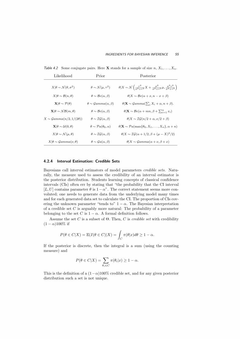
INGREDIENTS FOR BAYESIAN INFERENCE 55
Table 4.2 Some conjugate pairs. Here X stands for a sample of size n, X1, . . . , Xn.
Likelihood Prior Posterior
X|θ ∼ N (θ, σ2) θ ∼ N (µ, τ2) θ|X ∼ N“
τ2
σ2+τ2 X + σ2
σ2+τ2 µ, σ2τ2
σ2+τ2
”
X|θ ∼ B(n, θ) θ ∼ Be(α, β) θ|X ∼ Be(α + x, n− x + β)
X|θ ∼ P(θ) θ ∼ Gamma(α, β) θ|X ∼ Gamma(P
i Xi + α, n + β).
X|θ ∼ NB(m, θ) θ ∼ Be(α, β) θ|X ∼ Be(α + mn, β +Pn
i=1 xi)
X ∼ Gamma(n/2, 1/(2θ)) θ ∼ IG(α, β) θ|X ∼ IG(n/2 + α, x/2 + β)
X|θ ∼ U(0, θ) θ ∼ Pa(θ0, α) θ|X ∼ Pa(maxθ0, X1, . . . , Xn, α + n)
X|θ ∼ N (µ, θ) θ ∼ IG(α, β) θ|X ∼ IG(α + 1/2, β + (µ−X)2/2)
X|θ ∼ Gamma(ν, θ) θ ∼ Ga(α, β) θ|X ∼ Gamma(α + ν, β + x)
4.2.4 Interval Estimation: Credible Sets
Bayesians call interval estimators of model parameters credible sets. Natu-rally, the measure used to assess the credibility of an interval estimator isthe posterior distribution. Students learning concepts of classical confidenceintervals (CIs) often err by stating that “the probability that the CI interval[L,U ] contains parameter θ is 1−α”. The correct statement seems more con-voluted; one needs to generate data from the underlying model many timesand for each generated data set to calculate the CI. The proportion of CIs cov-ering the unknown parameter “tends to” 1− α. The Bayesian interpretationof a credible set C is arguably more natural: The probability of a parameterbelonging to the set C is 1− α. A formal definition follows.
Assume the set C is a subset of Θ. Then, C is credible set with credibility(1− α)100% if
P (θ ∈ C|X) = E(I(θ ∈ C)|X) =∫
C
π(θ|x)dθ ≥ 1− α.
If the posterior is discrete, then the integral is a sum (using the countingmeasure) and
P (θ ∈ C|X) =∑
θi∈C
π(θi|x) ≥ 1− α.
This is the definition of a (1−α)100% credible set, and for any given posteriordistribution such a set is not unique.

56 BAYESIAN STATISTICS
For a given credibility level (1−α)100%, the shortest credible set has obvi-ous appeal. To minimize size, the sets should correspond to highest posteriorprobability density areas (HPDs).
Definition 4.1 The (1 − α)100% HPD credible set for parameter θ is a setC, subset of Θ of the form
C = θ ∈ Θ|π(θ|x) ≥ k(α),
where k(α) is the largest constant for which
P (θ ∈ C|X) ≥ 1− α.
Geometrically, if the posterior density is cut by a horizontal line at thehight k(α), the set C is projection on the θ axis of the part of line that liesbelow the density.
Example 4.6 Jeremy’s IQ, Continued. Recall Jeremy, the enthusiasticGeorgia Tech student from Example 4.4, who used Bayesian inference in mod-eling his IQ test scores. For a score X|θ he was using a N (θ, 80) likelihood,while the prior on θ was N (110, 120). After the score of X = 98 was recorded,the resulting posterior was normal N (102.8, 48).
Here, the MLE is θ = 98, and a 95% confidence interval is [98−1.96√
80, 98+1.96
√80] = [80.4692, 115.5308]. The length of this interval is approximately
35. The Bayesian counterparts are θ = 102.8, and [102.8− 1.96√
48, 102.8 +1.96
√48] = [89.2207, 116.3793]. The length of 95% credible set is approxi-
mately 27. The Bayesian interval is shorter because the posterior variance issmaller than the likelihood variance; this is a consequence of the incorporationof information. The construction of the credible set is illustrated in Figure4.3.
4.2.5 Bayesian Testing
Bayesian tests amount to comparison of posterior probabilities of the param-eter regions defined by the two hypotheses.
Assume that Θ0 and Θ1 are two non-overlapping subsets of the parameterspace Θ. We assume that Θ0 and Θ1 partition Θ, that is, Θ1 = Θc
0, althoughcases in which Θ1 6= Θc
0 are easily formulated. Let θ ∈ Θ0 signify the nullhypothesis H0 and let θ ∈ Θ1 = Θc
0 signify the alternative hypothesis H1:
H0 : θ ∈ Θ0 H1 : θ ∈ Θ1.
Given the information from the posterior, the hypothesis with higher posteriorprobability is selected.
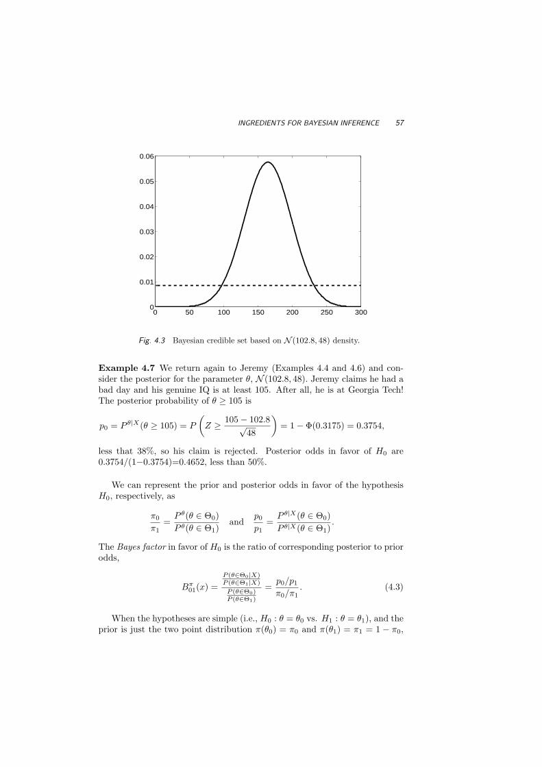
INGREDIENTS FOR BAYESIAN INFERENCE 57
0 50 100 150 200 250 3000
0.01
0.02
0.03
0.04
0.05
0.06
Fig. 4.3 Bayesian credible set based on N (102.8, 48) density.
Example 4.7 We return again to Jeremy (Examples 4.4 and 4.6) and con-sider the posterior for the parameter θ, N (102.8, 48). Jeremy claims he had abad day and his genuine IQ is at least 105. After all, he is at Georgia Tech!The posterior probability of θ ≥ 105 is
p0 = P θ|X(θ ≥ 105) = P
(Z ≥ 105− 102.8√
48
)= 1− Φ(0.3175) = 0.3754,
less that 38%, so his claim is rejected. Posterior odds in favor of H0 are0.3754/(1−0.3754)=0.4652, less than 50%.
We can represent the prior and posterior odds in favor of the hypothesisH0, respectively, as
π0
π1=
P θ(θ ∈ Θ0)P θ(θ ∈ Θ1)
andp0
p1=
P θ|X(θ ∈ Θ0)P θ|X(θ ∈ Θ1)
.
The Bayes factor in favor of H0 is the ratio of corresponding posterior to priorodds,
Bπ01(x) =
P (θ∈Θ0|X)P (θ∈Θ1|X)
P (θ∈Θ0)P (θ∈Θ1)
=p0/p1
π0/π1. (4.3)
When the hypotheses are simple (i.e., H0 : θ = θ0 vs. H1 : θ = θ1), and theprior is just the two point distribution π(θ0) = π0 and π(θ1) = π1 = 1 − π0,
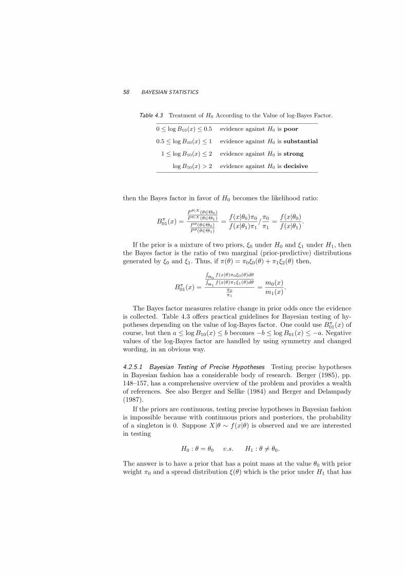
58 BAYESIAN STATISTICS
Table 4.3 Treatment of H0 According to the Value of log-Bayes Factor.
0 ≤ log B10(x) ≤ 0.5 evidence against H0 is poor
0.5 ≤ log B10(x) ≤ 1 evidence against H0 is substantial
1 ≤ log B10(x) ≤ 2 evidence against H0 is strong
log B10(x) > 2 evidence against H0 is decisive
then the Bayes factor in favor of H0 becomes the likelihood ratio:
Bπ01(x) =
P θ|X(θ∈Θ0)P θ|X(θ∈Θ1)
P θ(θ∈Θ0)P θ(θ∈Θ1)
=f(x|θ0)π0
f(x|θ1)π1/π0
π1=
f(x|θ0)f(x|θ1)
.
If the prior is a mixture of two priors, ξ0 under H0 and ξ1 under H1, thenthe Bayes factor is the ratio of two marginal (prior-predictive) distributionsgenerated by ξ0 and ξ1. Thus, if π(θ) = π0ξ0(θ) + π1ξ2(θ) then,
Bπ01(x) =
RΘ0
f(x|θ)π0ξ0(θ)dθRΘ1
f(x|θ)π1ξ1(θ)dθ
π0π1
=m0(x)m1(x)
.
The Bayes factor measures relative change in prior odds once the evidenceis collected. Table 4.3 offers practical guidelines for Bayesian testing of hy-potheses depending on the value of log-Bayes factor. One could use Bπ
01(x) ofcourse, but then a ≤ log B10(x) ≤ b becomes −b ≤ log B01(x) ≤ −a. Negativevalues of the log-Bayes factor are handled by using symmetry and changedwording, in an obvious way.
4.2.5.1 Bayesian Testing of Precise Hypotheses Testing precise hypothesesin Bayesian fashion has a considerable body of research. Berger (1985), pp.148–157, has a comprehensive overview of the problem and provides a wealthof references. See also Berger and Sellke (1984) and Berger and Delampady(1987).
If the priors are continuous, testing precise hypotheses in Bayesian fashionis impossible because with continuous priors and posteriors, the probabilityof a singleton is 0. Suppose X|θ ∼ f(x|θ) is observed and we are interestedin testing
H0 : θ = θ0 v.s. H1 : θ 6= θ0.
The answer is to have a prior that has a point mass at the value θ0 with priorweight π0 and a spread distribution ξ(θ) which is the prior under H1 that has

INGREDIENTS FOR BAYESIAN INFERENCE 59
prior weight π1 = 1− π0. Thus, the prior is the 2-point mixture
π(θ) = π0δθ0 + π1ξ(θ),
where δθ0 is Dirac mass at θ0.
The marginal density for X is
m(x) = π0f(x|θ0) + π1
∫f(x|θ)ξ(θ)dθ = π0f(x|θ0) + π1m1(x).
The posterior probability of θ = θ0 is
π(θ0|x) = f(x|θ0)π0/m(x) =f(x|θ0)π0
π0f(x|θ0) + π1m1(x)=
(1 +
π1
π0· m1(x)f(x|θ0)
)−1
.
4.2.6 Bayesian Prediction
Statistical prediction fits naturally into the Bayesian framework. SupposeY ∼ f(y|θ) is to be observed. The posterior predictive distribution of Y ,given observed X = x is
f(y|x) =∫
Θ
f(y|θ)π(θ|x)dθ.
For example, in the normal distribution example, the predictive distributionof Y , given X1, . . . , Xn is
Y |X ∼ N(
τ2
σ2
n + τ2X +
σ2
nσ2
n + τ2µ, σ2 +
σ2
n τ2
σ2
n + τ2
). (4.4)
Example 4.8 Martz and Waller (1985) suggest that Bayesian reliabilityinference is most helpful in applications where little system failure data exist,but past data from like systems are considered relevant to the present system.They use an example of heat exchanger reliability, where the lifetime X is thefailure time for heat exchangers used in refining gasoline. From past researchand modeling in this area, it is determined that X has a Weibull distributionwith κ = 3.5. Furthermore, the scale parameter λ is considered to be in theinterval 0.5 ≤ λ ≤ 1.5 with no particular value of λ considered more likelythan others.
From this argument, we have
π(λ) =
1 0.5 ≤ λ ≤ 1.50 otherwise
f(x|λ) = κλκxκ−1e−(xλ)κ

60 BAYESIAN STATISTICS
where κ = 3.5. With n=9 observed failure times (measured in years of service)at (0.41, 0.58, 0.75, 0.83, 1.00, 1.08, 1.17, 1.25, 1.35), the likelihood is
f(x1, . . . , x9|λ) ∝ λp
(9∏
i=1
xi2.5
)e−λ3.5(
Pxi
3.5),
so the sufficient statistic isn∑
i=1
xi3.5 = 10.16.
The resulting posterior distribution is not distributed Weibull (like the likeli-hood) or uniform (like the prior). It can be expressed as
π(λ|x1, . . . , x9) =
(1621.39)λ9e−10.16λ3.50.5 ≤ λ ≤ 1.5
0 otherwise,
and has expected value of λB = 0.6896. Figure 4.4(a) shows the posterior den-sity From the prior distribution, E(λ) = 1, so our estimate of λ has decreasedin the process of updating the prior with the data.
0.2 0.4 0.6 0.8 1 1.2 1.4
0.5
1
1.5
2
2.5
3
3.5
0.2 0.4 0.6 0.8 1 1.2 1.4
0.5
1
1.5
2
2.5
3
3.5
1 2 3 4
0.2
0.4
0.6
0.8
(a) (b)
Fig. 4.4 (a) Posterior density for λ; (b) Posterior predictive density for heat-exchanger lifetime.
Estimation of λ was not the focus of this study; the analysts were interestedin predicting future lifetime of a generic (randomly picked) heat exchanger.Using the predictive density from (4.4),
f(y|x) =∫ 1.5
0.5
(3.5λ3.5y2.5e−(λy)3.5
)(1621.39λ9e−10.16λ3.5
)dλ.

BAYESIAN COMPUTATION AND USE OF WINBUGS 61
The predictive density is a bit messy, but straightforward to work with.The plot of the density in Figure 4.4(b) shows how uncertainty is gauged forthe lifetime of a new heat-exchanger. From f(y|x), we might be interestedin predicting early failure by the new item; for example, a 95% lower boundfor heat-exchanger lifetime is found by computing the lower 0.05-quantile off(y|x), which is approximately 0.49.
4.3 BAYESIAN COMPUTATION AND USE OF WINBUGS
If the selection of an adequate prior was the major conceptual and modelingchallenge of Bayesian analysis, the major implementational challenge is com-putation. When the model deviates from the conjugate structure, finding theposterior distribution and the Bayes rule is all but simple. A closed form so-lution is more an exception than the rule, and even for such exceptions, luckymathematical coincidences, convenient mixtures, and other tricks are neededto uncover the explicit expression.
If the classical statistics relies on optimization, Bayesian statistics relieson integration. The marginal needed for the posterior is an integral
m(x) =∫
Θ
f(x|θ)π(θ)dθ,
and the Bayes estimator of h(θ), with respect to the squared error loss is aratio of integrals,
δπ(x) =∫
Θ
h(θ)π(θ|x)dθ =
∫Θ
h(θ)f(x|θ)π(θ)dθ∫Θ
f(x|θ)π(θ)dθ.
The difficulties in calculating the above Bayes rule come from the facts that(i) the posterior may not be representable in a finite form, and (ii) the integralof h(θ) does not have a closed form even when the posterior distribution isexplicit.
The last two decades of research in Bayesian statistics contributed tobroadening the scope of Bayesian models. Models that could not be han-dled before by a computer are now routinely solved. This is done by Markovchain Monte Carlo (MCMC) Methods, and their introduction to the field ofstatistics revolutionized Bayesian statistics.
The Markov chain Monte Carlo (MCMC) methodology was first appliedin statistical physics, (Metropolis et al., 1953). Work by Gelfand and Smith(1990) focused on applications of MCMC to Bayesian models. The principleof MCMC is simple: to sample randomly from a target probability distribu-tion one designs a Markov chain whose stationary distribution is the targetdistribution. By simulating long runs of such a Markov chain, the targetdistribution can be well approximated. Various strategies for constructing

62 BAYESIAN STATISTICS
appropriate Markov chains that simulate form the desired distribution arepossible: Metropolis-Hastings, Gibbs sapmler, slice sampling, perfect sam-pling, and many specialized techniques. They are beyond the scope of thistext and the interested reader is directed to Robert (2001), Robert and Casella(2004), and Chen, Shao, and Ibrahim (2000), for an overview and a compre-hensive treatment.
We will use WinBUGS for doing Bayesian inference on non conjugatemodels. Appendix B offers a brief introduction to the front-end of Win-BUGS. Three volumes of examples are standard addition to the software, inthe Examples menu of WinBUGS, see Spiegelhalter, Thomas, Best, and Gilks(1996). It is recommended that you go over some of those in detail becausethey illustrate the functionality and real modeling power of WinBUGS. Awealth of examples on Bayesian modeling strategies using WinBUGS can befound in the monographs of Congdon (2001, 2003, 2005). The following ex-ample demonstrates the simulation power of WinBUGS, although it involvesapproximating probabilities of complex events and has nothing to do withBayesian inference.
Example 4.9 Paradox DeMere in WinBUGS. In 1654 the Chevalierde Mere asked Blaise Pascal (1623–1662) the following question: In playinga game with three dice why the sum 11 is advantageous to sum 12 when bothare results of six possible outcomes? Indeed, there are six favorable tripletsfor each of the sums 11 and 12,
11: (1, 4, 6), (1, 5, 5), (2, 3, 6), (2, 4, 5), (3, 3, 5), (3, 4, 4)12: (1, 5, 6), (2, 4, 6), (2, 5, 5), (3, 3, 6), (3, 4, 5), (4, 4, 4)
The solution to this “paradox” deMere is simple. By taking into account allpossible permutations of the triples, the sum 11 has 27 favorable permutationswhile the sum 12 has 25 favorable permutation. But what if 300 fair dice arerolled and we are interested if the sum 1111 is advantageous to the sum 1112?Exact solution is unappealing, but the probabilities can be well approximatedby WinBUGS model demere1.
model demere1;
for (i in 1:300)
dice[i] ~ dcat(p.dice[]);
is1111 <- equals(sum(dice[]),1111)
is1112 <- equals(sum(dice[]),1112)
The data are
list(p.dice=c(0.1666666, 0.1666666,
0.1666667, 0.1666667, 0.1666667, 0.1666667) )

EXERCISES 63
and the initial values are generated. After five million rolls, WinBUGS outputsis1111 = 0.0016 and is1112 = 0.0015, so the sum of 1111 is advantageousto the sum of 1112.
Example 4.10 Jeremy in WinBUGS. We will calculate a Bayes estima-tor for Jeremy’s true IQ using BUGS. Recall, the model in Example 4.4 wasX ∼ N (θ, 80) and θ ∼ N (100, 120). In WinBUGS we will use the precisionparameters 1/120 = 0.00833 and 1/80 = 0.0125.
#Jeremy in WinBUGS
model
x ~ dnorm( theta, tau)
theta ~ dnorm( 110, 0.008333333)
#data
list( tau=0.0125, x=98)
#inits
list(theta=100)
Below is the summary of MCMC output.
node mean sd MC error 2.5% median 97.5%
θ 102.8 6.917 0.0214 89.17 102.8 116.3
Because this is a conjugate normal/normal model, the exact posterior dis-tribution, N (102.8, 48), was easy to find, (see Example 4.4). Note that insimulations, the MCMC approximation, when rounded, coincides with theexact posterior mean. The MCMC variance of θ is 6.9172 = 47.84489, closeto the exact posterior variance of 48.
4.4 EXERCISES
4.1. A lifetime X (in years) of a particular machine is modeled by an exponen-tial distribution with unknown failure rate parameter θ. The lifetimesof X1 = 5, X2 = 6, and X3 = 4 are observed, and assume that an expertbelieves that θ should have exponential distribution as well and that,on average θ should be 1/3.
(i) Write down the MLE of θ for those observations.
(ii) Elicit a prior according to the expert’s beliefs.
(iii) For the prior in (ii), find the posterior. Is the problem conjugate?
(iv) Find the Bayes estimator θBayes, and compare it with the MLEestimator from (i). Discuss.
64 BAYESIAN STATISTICS
4.2. Suppose X = (X1, . . . , Xn) is a sample from U(0, θ). Let θ have ParetoPa(θ0, α) distribution. Show that the posterior distribution is Pa(maxθ0,x1, . . . , xn α + n).
4.3. Let X ∼ G(n/2, 2θ), so that X/θ is χ2n. Let θ ∼ IG(α, β). Show that
the posterior is IG(n/2 + α, (x/2 + β−1)−1).
4.4. If X = (X1, . . . , Xn) is a sample from NB(m, θ) and θ ∼ Be(α, β), showthat the posterior for θ is beta Be(α + mn, β +
∑ni=1 xi).
4.5. In Example 4.5 on p. 54, show that the marginal distribution is negativebinomial.
4.6. What is the Bayes factor Bπ01 in Jeremy’s case (Example 4.7)? Test H0
is using the Bayes factor and wording from the Table 4.3. Argue thatthe evidence against H0 is poor.
4.7. Assume X|θ ∼ N (θ, σ2) and θ ∼ π(θ) = 1. Consider testing H0 : θ ≤ θ0
v.s. H1 : θ > θ0. Show that p0 = P θ|X(θ ≤ θ0) is equal to the classicalp-value.
4.8. Show that the Bayes factor is Bπ01(x) = f(x|θ0)/m1(x).
4.9. Show that
p0 = π(θ0|x) ≥[1 +
π1
π0· r(x)f(x|θ0)
]−1
,
where r(x) = supθ 6=θ0f(x|θ). Usually, r(x) = f(x|θMLE), where θmle is
MLE estimator of θ. The Bayes factor Bπ01(x) is bounded from below:
Bπ01(x) ≥ f(x|θ0)
r(x)=
f(x|θ0)
f(x|θMLE).
4.10. Suppose X = −2 was observed from the population distributed asN(0, 1/θ) and one wishes to estimate the parameter θ. (Here θ is thereciprocal of variance σ2 and is called the precision parameter. Theprecision parameter is used in WinBUGS to parameterize the normaldistribution). A classical estimator of θ (e.g., the MLE) does exist, butone may be disturbed to estimate 1/σ2 based on a single observation.Suppose the analyst believes that the prior on θ is Gamma(1/2, 3).
(i) What is the MLE of θ?
(ii) Find the posterior distribution and the Bayes estimator of θ. If theprior on θ is Gamma(α, β), represent the Bayes estimator as weightedaverage (sum of weights = 1) of the prior mean and the MLE.
(iii) Find a 95% HPD Credible set for θ.
(iv) Test the hypothesis H0 : θ ≤ 1/4 versus H1 : θ > 1/4.

EXERCISES 65
4.11. The Lindley (1957) Paradox. Suppose y|θ ∼ N(θ, 1/n). We wish to testH0 : θ = 0 versus the two sided alternative. Suppose a Bayesian putsthe prior P (θ = 0) = P (θ 6= 0) = 1/2, and in the case of the alternative,the 1/2 is uniformly spread over the interval [−M/2,M/2]. Supposen = 40, 000 and y = 0.01 are observed, so
√n y = 2. The classical
statistician rejects H0 at level α = 0.05. Show that posterior odds infavor of H0 are 11 if M = 1, indicating that a Bayesian statisticianstrongly favors H0, according to Table 4.3.
4.12. This exercise concerning Bayesian binary regression with a probit modelusing WinBUGS is borrowed from David Madigan’s Bayesian CourseSite. Finney (1947) describes a binary regression problem with data ofsize n = 39, two continuous predictors x1 and x2, and a binary responsey. Here are the data in BUGS-ready format:
list(n=39,x1=c(3.7,3.5,1.25,0.75,0.8,0.7,0.6,1.1,0.9,0.9,0.8,0.55,0.6,1.4,
0.75,2.3,3.2,0.85,1.7,1.8,0.4,0.95,1.35,1.5,1.6,0.6,1.8,0.95,1.9,1.6,2.7,
2.35,1.1,1.1,1.2,0.8,0.95,0.75,1.3),
x2=c(0.825,1.09,2.5,1.5,3.2,3.5,0.75,1.7,0.75,0.45,0.57,2.75,3.0,2.33,3.75,
1.64,1.6,1.415,1.06,1.8,2.0,1.36,1.35,1.36,1.78,1.5,1.5,1.9,0.95,0.4,0.75,
0.03,1.83,2.2,2.0,3.33,1.9,1.9,1.625),
y=c(1,1,1,1,1,1,0,0,0,0,0,0,0,1,1,1,1,1,0,1,0,0,0,0,1,0,1,0,1,0,1,0,0,1,1,
1,0,0,1))
The objective is to build a predictive model that predicts y from x1
and x2. Proposed approach is the probit model: P (y = 1|x1, x2) =Φ(β0 + β1 x1 + β2 x2) where Φ is the standard normal CDF.
(i) Use WinBUGS to compute posterior distributions for β0, β1 and β2
using diffuse normal priors for each.
(ii) Suppose instead of the diffuse normal prior for βi, i = 0, 1, 2, youuse a normal prior with mean zero and variance vi, and assume the visare independently exponentially distributed with some hyperparameterγ. Fit this model using BUGS. How different are the two posteriordistributions from this exercise?
4.13. The following WinBUGS code flips a coin, the outcome H is coded by1 and tails by 0. Mimic the following code to simulate a rolling of a fairdie.
#coin.bug:
model coin;
flip12 ~ dcat(p.coin[])
coin <- flip12 - 1
#coin.dat:
list(p.coin=c(0.5, 0.5))
# just generate initials

66 BAYESIAN STATISTICS
4.14. The highly publicized (recent TV reports) in vitro fertilization successcases for women in their late fifties all involve donor’s egg. If the egg isthe woman’s own, the story is quite different.
In vitro fertilization (IVF), one of the assisted reproductive technology(ART) procedures, involves extracting a woman’s eggs, fertilizing theeggs in the laboratory, and then transferring the resulting embryos intothe womans uterus through the cervix. Fertilization involves a special-ized technique known as intracytoplasmic sperm injection (ICSI).
The table shows the live-birth success rate per transfer rate from therecipients’ eggs, stratified by age of recipient. The data are for year1999, published by US - Centers for Disease Control and Prevention(CDC): (http://www.cdc.gov/reproductivehealth/ART99/index99.htm )
Age (x) 24 25 26 27 28 29 30 31Percentage (y) 38.7 38.6 38.9 41.4 39.7 41.1 38.7 37.6
Age (x) 32 33 34 35 36 37 38 39Percentage(y) 36.3 36.9 35.7 33.8 33.2 30.1 27.8 22.7
Age (x) 40 41 42 43 44 45 46Percentage(y) 21.3 15.4 11.2 9.2 5.4 3.0 1.6
Assume the change-point regression model
yi = β0 + β1xi + εi, i = 1, . . . , τ
yi = γ0 + γ1xi + εi, i = τ + 1, . . . , n
εi ∼ N (0, σ2).
(i) Propose priors (with possibly hyperpriors) on σ2, β0, β1, γ0, and γ1.
(ii) Take discrete uniform prior on τ and write a WinBUGS program.
4.15. Is the cloning of humans moral? Recent Gallup Poll estimates thatabout 88% Americans opposed cloning humans. Results are based ontelephone interviews with a randomly selected national sample of n =1000 adults, aged 18 and older, conducted May 2-4, 2004. In these 1000interviews, 882 adults opposed cloning humans.
(i) Write WinBUGS program to estimate the proportion p of peopleopposed to cloning humans. Use a non-informative prior for p.
(ii) Test the hypothesis that p ≤ 0.87.(iii) Pretend that the original poll had n = 1062 adults, i.e., resultsfor 62 adults are missing. Estimate the number of people opposed tocloning among the 62 missing in the poll. Hint:
model anticlons ~ dbin(prob,npolled) ;

REFERENCES 67
lessthan87 <- step(prob-0.87)
anticlons.missing ~ dbin(prob,nmissing)
prob ~ dbeta(1,1)
Data
list(anticlons=882,npolled= 1000, nmissing=62)
REFERENCES
Anscombe, F. J. (1962), “Tests of Goodness of Fit,” Journal of the RoyalStatistical Society (B), 25, 81-94.
Bayes, T. (1763), “An Essay Towards Solving a Problem in the Doctrine ofChances,” Philosophical Transactions of the Royal Society, London, 53,370-418.
Berger, J. O. (1985), Statistical Decision Theory and Bayesian Analysis, Sec-ond Edition, New York: Springer-Verlag.
Berger, J. O., and Delampady, M. (1987), “Testing Precise Hypothesis,” Sta-tistical Science, 2, 317-352.
Berger, J. O., and Selke, T. (1987), “Testing a Point Null Hypothesis: TheIrreconcilability of p-values and Evidence (with Discussion)”, Journal ofAmerican Statistical Association, 82, 112-122.
Chen, M.-H., Shao, Q.-M., and Ibrahim, J. (2000), Monte Carlo Methods inBayesian Computation, New York: Springer Verlag.
Congdon, P. (2001), Bayesian Statistical Modelling, Hoboken, NJ: Wiley.Congdon, P. (2003), Applied Bayesian Models, Hoboken, NJ: Wiley.Congdon, P. (2005), Bayesian Models for Categorical Data, Hoboken, NJ:
Wiley.Finney, D. J. (1947), “The Estimation from Individual Records of the Rela-
tionship Between Dose and Quantal Response,” Biometrika, 34, 320-334.Gelfand, A. E., and Smith, A. F. M. (1990), “Sampling-based Approaches to
Calculating Marginal Densities,” Journal of American Statistical Asso-ciation, 85, 398-409.
Lindley, D. V. (1957), “A Statistical Paradox,” Biometrika, 44, 187-192.Madigan, D. http://stat.rutgers.edu/ madigan/bayes02/. A Web Site
for Course on Bayesian Statistics.Martz, H., and Waller, R. (1985), Bayesian Reliability Analysis, New York:
Wiley.Metropolis, N., Rosenbluth, A., Rosenbluth, M., Teller, A., and Teller, E.
(1953), “Equation of State Calculations by Fast Computing Machines,”The Journal of Chemical Physics, 21, 1087-1092.

68 BAYESIAN STATISTICS
Robert, C. (2001), The Bayesian Choice: From Decision-Theoretic Moti-vations to Computational Implementation, Second Edition, New York:Springer Verlag.
Robert, C. and Casella, G. (2004), Monte Carlo Statistical Methods, SecondEdition, New York: Springer Verlag.
Spiegelhalter, D. J., Thomas, A., Best, N. G., and Gilks, W. R. (1996), “BUGSExamples Volume 1,” Version 0.5. Cambridge: Medical Research CouncilBiostatistics Unit (PDF).

5Order Statistics
The early bird gets the worm, but the second mouse gets the cheese.
Steven Wright
Let X1, X2, . . . , Xn be an independent sample from a population with ab-solutely continuous cumulative distribution function F and density f. Thecontinuity of F implies that P (Xi = Xj) = 0, when i 6= j and the samplecould be ordered with strict inequalities,
X1:n < X2:n < · · · < Xn−1:n < Xn:n, (5.1)
where Xi:n is called the ith order statistic (out of n). The range of the datais Xn:n −X1:n, where Xn:n and X1:n are, respectively, the sample maximumand minimum. The study of order statistics permeates through all areas ofstatistics, including nonparametric. There are several books dedicated just toprobability and statistics related to order statistics; the textbook by Davidand Nagaraja (2003) is a deservedly popular choice.
The marginal distribution of Xi:n is not the same as Xi. Its distributionfunction Fi:n(t) = P (Xi:n ≤ t) is the probability that at least i out of nobservations from the original sample are no greater than t, or
Fi:n(t) = P (Xi:n ≤ t) =n∑
k=i
(n
k
)F (t)k (1− F (t))n−k
.
If F is differentiable, it is possible to show that the corresponding density
69

70 ORDER STATISTICS
function is
fi:n(t) = i
(n
i
)F (t)i−1 (1− F (t))n−i
f(t). (5.2)
Example 5.1 Recall that for any continuous distribution F , the transformedsample F (X1), . . . , F (Xn) is distributed U(0, 1). Similarly, from (5.2) thedistribution of F (Xi:n) is Be(i, n − i + 1). Using the MATLAB code below,the densities are graphed in Figure 5.1.
>> x=0:0.025:1;
>> for i=1,5
>> plot(betapdf(x,i,6-i))
>> hold all
>> end
Example 5.2 Reliability Systems. In reliability, series and parallel sys-tems are building blocks for system analysis and design. A series system is onethat works only if all of its components are working. A parallel system is onethat fails only if all of its components fail. If the lifetimes of a n-componentsystem (X1, . . . , Xn) are i.i.d. distributed, then if the system is in series, thesystem lifetime is X1:n. On the other hand, for a parallel system, the lifetimeis Xn:n.
5.1 JOINT DISTRIBUTIONS OF ORDER STATISTICS
Unlike the original sample (X1, X2, . . . , Xn), the set of order statistics is in-evitably dependent. If the vector (X1, X2, . . . , Xn) has a joint density
f1,2,...,n(x1, x2, . . . , xn) =n∏
i=1
f(xi),
then the joint density for the order statistics, f1,2,...,n:n(x1, ..., xn) is
f1,2,...,n:n(x1, ..., xn) =
n!∏n
i=1 f(xi) x1 < x2 < · · · < xn
0 otherwise. (5.3)
To understand why this is true, consider the conditional distribution ofthe order statistics y = (x1:n, x2:n, . . . , xn:n) given x = (x1, x2, . . . , xn). Eachone of the n! permutations of (X1, X2, . . . , Xn) are equal in probability, socomputing fy =
∫fy|xdFx is incidental. The joint density can also be derived
using a Jacobian transformation (see Exercise 5.3).

JOINT DISTRIBUTIONS OF ORDER STATISTICS 71
0 0.2 0.4 0.6 0.8 10
0.5
1
1.5
2
2.5
3
3.5
4
4.5
5
Fig. 5.1 Distribution of order statistics from a sample of five U(0, 1).
From (5.3) we can obtain the distribution of any subset of order statistics.The joint distribution of Xr:n, Xs:n, 1 ≤ r < s ≤ n is defined as
Fr,s:n(xr, xs) = P (Xr:n ≤ xr, Xs:n ≤ xs),
which is the probability that at least r out of n observations are at most xr,and at least s of n observations are at most xs. The probability that exactlyi observations are at most xr and j are at most xs is
n!(i− 1)!(j − i)!(n− j)!
F (xr)i (F (xs)− F (xr))j−i (1− F (xs))
n−j,
where −∞ < xr < xs < ∞; hence
Fr,s:n(xr, xs) =n∑
j=s
s∑
i=r
n!(i− 1)!(j − i)!(n− j)!
×
F (xr)i (F (xs)− F (xr))j−i (1− F (xs))
n−j. (5.4)
If F is differentiable, it is possible to formulate the joint density of two order
72 ORDER STATISTICS
statistics as
fr,s:n(xr, xs) =n!
(r − 1)!(s− r − 1)!(n− s)!× (5.5)
F (xr)r−1 (F (xs)− F (xr))s−r−1 (1− F (xs))
n−sf(xr)f(xs).
Example 5.3 Sample Range. The range of the sample, R, defined beforeas Xn:n −X1:n, has density
fR(u) =∫ ∞
−∞n(n− 1)[F (v)− F (v − u)]n−2f(v − u)f(v)dv. (5.6)
To find fR(u), start with the joint distribution of (X1:n, Xn:n) in (5.5),
f1,n:n(y1, yn) = n(n− 1)[F (yn)− F (y1)]n−2f(y1)f(yn).
and make the transformation
u = yn − y1
v = yn.
The Jacobian of this transformation is 1, and y1 = v − u, yn = v. Plug y1, yn
into the joint distribution f1,n:n(y1, yn) and integrate out v to arrive at (5.6).For the special case in which F (t) = t, the probability density function forthe sample range simplifies to
fR(u) = n(n− 1)un−2(1− u), 0 < u < 1.
5.2 SAMPLE QUANTILES
Recall that for a distribution F , the pth quantile (xp) is the value x suchthat F (x) = p, if the distribution is continuous, and more generally, suchthat F (x) ≥ p and P (X ≥ x) ≥ 1 − p, if the distribution is arbitrary. Forexample, if the distribution F is discrete, there may not be any value x forwhich F (x) = p.
Analogously, if X1, . . . , Xn represents a sample from F , the pth samplequantile (xp) is a value of x such that 100p% of the sample is smaller than x.This is also called the 100p% sample percentile. With large samples, there isa number 1 ≤ r ≤ n such that Xr:n ≈ xp. Specifically, if n is large enoughso that p(n + 1) = r for some r ∈ Z, then xp = Xr:n because there would ber − 1 values smaller than xp in the sample, and n− r larger than it.
If p(n + 1) is not an integer, we can consider estimating the populationquantile by an inner point between two order statistics, say Xr:n and X(r+1):n,

TOLERANCE INTERVALS 73
where F (Xr:n) < p− ε and F (X(r+1):n) > p + ε for some small ε > 0. In thiscase, we can use a number that interpolates the value of xp using the linebetween (Xr:n, r/(n + 1)) and (X(r+1):n, (r + 1)/(n + 1)):
xp = (−p(n + 1) + r + 1) Xr:n + (p(n + 1)− r)X(r+1):n. (5.7)
Note that if p = 1/2 and n is an even number, then r = n/2 and r+1 = n/2+1,and xp = (Xn
2 :n + X( n2 +1):n)/2. That is, the sample median is the average of
the two middle sample order statistics.We note that there are alternative definitions of sample quantile in the
literature, but they all have the same large sample properties.
5.3 TOLERANCE INTERVALS
Unlike the confidence interval, which is constructed to contain an unknownparameter with some specified degree of uncertainty (say, 1− γ), a toleranceinterval contains at least a proportion p of the population with probability γ.That is, a tolerance interval is a confidence interval for a distribution. Bothp, the proportion of coverage, and 1− γ, the uncertainty associated with theconfidence statement, are predefined probabilities. For instance, we may be95% confident that 90% of the population will fall within the range specifiedby a tolerance interval.
Order statistics play an important role in the construction of toleranceintervals. From a sample X1, . . . , Xn from (continuous) distribution F , twostatistics T1 < T2 represent a 100γ percent tolerance interval for 100p percentof the distribution F if
P (F (T2)− F (T1) ≥ p) ≥ γ.
Obviously, the distribution F (T2) − F (T1) should not depend on F . Recallthat for an order statistic Xi:n, Ui:n ≡ F (Xi:n) is distributed Be(i, n− i + 1).Choosing T1 and T2 from the set of order statistics satisfies the requirementsof the tolerance interval and the computations are not difficult.
One-sided tolerance intervals are related to confidence intervals for quan-tiles. For instance, a 90% upper tolerance bound for 95% of the population isidentical to a 90% one-sided confidence interval for x0.95, the 0.95 quantile ofthe distribution. With a sample of x1, . . . , xn from F , a γ interval for 100p%of the population would be constructed as (−∞, xr:n) for some r ∈ 1, . . . , n.
74 ORDER STATISTICS
Here are four simple steps to help determine r:
1. We seek r so that P (−∞ < xp < Xr:n) = γ = P (Xr:n > xp)
2. At most r − 1 out of n observations are less than xp
3. Let Y = number of observations less than xp. so that Y ∼ Bin(n, p) ifxp is the pth quantile
4. Find r large enough so that P (Y ≤ r − 1) = γ.
Example 5.4 A 90% upper confidence bound for the 75th percentile (orupper quartile) is found by assigning Y = number of observations less thanx0.75, where Y ∼ Bin(n, 0.75). Let n = 20. Note P (Y ≤ 16) = 0.7748 andP (Y ≤ 17) = 0.9087, so r − 1 = 17. The 90% upper bound for x0.75, whichis equivalent to a 90% upper tolerance bound for 75% of the population, isx18:20 (the third largest observation out of 20).
For large samples, the normal approximation allows us to generate anupper bound more simply. For the upper bound xr:n, r is approximated with
r = np + zγ
√np(1− p).
In the example above, with n = 20 (of course, this is not exactly what wethink of as “large”), r = 20(0.75) + 1.28
√0.75(0.25)20 = 17.48. According to
this rule, x17:20 is insufficient for the approximate interval, so x18:20 is againthe upper bound.
Example 5.5 Sample Range. From a sample of n, what is the probabilitythat 100p% of the population lies within the sample range (X1:n, Xn:n)?
P (F (Xn:n)− F (X1:n) ≥ p) = 1− P (Un < p)
where Un = Un:n − U1:n. From (5.6) it was shown that Un ∼ Be(n− 1, 2). Ifwe let γ = P (Un ≥ p), then γ, the tolerance coefficient can be solved
1− γ = npn−1 − (n− 1)pn.
Example 5.6 The tolerance interval is especially useful in compliance moni-toring at industrial sites. Suppose one is interested in maximum contaminantlevels (MCLs). The tolerance interval already takes into account the fact thatsome values will be high. So if a few values exceed the MCL standard, a sitemay still not be in violation (because the calculated tolerance interval maystill be lower than the MCL). But if too many values are above the MCL,the calculated tolerance interval will extend beyond the acceptable standard.

ASYMPTOTIC DISTRIBUTIONS OF ORDER STATISTICS 75
As few as three data points can be used to generate a tolerance interval, butthe EPA recommends having at least eight points for the interval to have anyusefulness (EPA/530-R-93-003).
Example 5.7 How large must a sample size n be so that at least 75% ofthe contamination levels are between X2:n and X(n−1):n with probability ofat least 0.95? If we follow the approach above, the distribution of Vn =U(n−1):n − U2:n is Be ((n− 1)− 2, n− (n− 1) + 2 + 1) = Be(n − 3, 4). Weneed n so that P (Vn ≥ 0.75) = betainc(0.25,4,n-3) ≥ 0.95 which occursas long as n ≥ 29.
5.4 ASYMPTOTIC DISTRIBUTIONS OF ORDER STATISTICS
Let Xr:n be rth order statistic in a sample of size n from a population withan absolutely continuous distribution function F having a density f . Letr/n → p, when n →∞. Then
√n
p(1− p)f(xp)(Xr:n − xp) =⇒ N (0, 1),
where xp is pth quantile of F , i.e., F (xp) = p.
Let Xr:n and Xs:n be rth and sth order statistics (r < s) in the sample ofsize n. Let r/n → p1 and s/n → p2, when n →∞. Then, for large n,
(Xr:n
Xs:n
)appr∼ N
([xp1
xp2
],Σ
),
where
Σ =[
p1(1− p1)[f(xp1)]−2/n p1(1− p2)/[nf(xp1)f(xp2)]
−1
p1(1− p2)/[nf(xp1)f(xp2)]−1 p2(1− p2)[f(xp2)]
−2/n
]
and xpi is pith quantile of F .
Example 5.8 Let r = n/2 so we are estimating the population median withx.50 = x(n/2):n. If f(x) = θ exp(−θx), for x > 0, then x0.50 = ln(2)/θ and
√n (x0.50 − x0.50) =⇒ N (
0, θ−2).

76 ORDER STATISTICS
5.5 EXTREME VALUE THEORY
Earlier we equated a series system lifetime (of n i.i.d. components) with thesample minimum X1:n. The limiting distribution of the minima or maximaare not so interesting, e.g., if X has distribution function F , X1:n → x0,where x0 = infxx : F (x) > 0. However, the standardized limit is moreinteresting. For an example involving sample maxima, with X1, ..., Xn froman exponential distribution with mean 1, consider the asymptotic distributionof Xn:n − log(n):
P (Xn:n − log(n) ≤ t)) = P (Xn:n ≤ t + log(n)) = [1− exp−t− log(n)]n= [1− e−tn−1]n → exp−e−t.
This is because (1 + α/n)n → eα as n →∞. This distribution, a special formof the Gumbel distribution, is also called the extreme-value distribution.
Extreme value theory states that the standardized series system lifetimeconverges to one of the three following distribution types F ∗ (not includingscale and location transformation) as the number of components increases toinfinity:
Gumbel F ∗(x) = exp(− exp(−x)), −∞ < x < ∞
Frechet F ∗(x) =
exp(−x−a), x > 0, a > 00, x ≤ 0
Negative Weibull F ∗(x) =
exp(−(−x)a), x < 0, a > 00, x ≥ 0
5.6 RANKED SET SAMPLING
Suppose a researcher is sent out to Leech Lake, Minnesota, to ascertain theaverage weight of Walleye fish caught from that lake. She obtains her data bystopping the fishermen as they are returning to the dock after a day of fishing.In the time the researcher waited at the dock, three fishermen arrived, eachwith their daily limit of three Walleye. Because of limited time, she only hastime to make one measurement with each fisherman, so at the end of her fieldstudy, she will get three measurements.
McIntyre (1952) discovered that with this forced limitation on measure-ments, there is an efficient way of getting information about the populationmean. We might assume the researcher selected the fish to be measured ran-
EXERCISES 77
domly for each of the three fishermen that were returning to shore. McIntyrefound that if she instead inspected the fish visually and selected them non-randomly, the data could beget a better estimator for the mean. Specifically,suppose the researcher examines the three Walleye from the first fishermanand selects the smallest one for measurement. She measures the second small-est from the next batch, and the largest from the third batch.
Opposed to a simple random sample (SRS), this ranked set sample (RSS)consists of independent order statistics which we will denote by X[1:3], X[2:3],X[3:3]. If X is the sample mean from a SRS of size n, and XRSS is the meanof a ranked set sample X[1:n], . . . , X[n:n], it is easy to show that like X, XRSS
is an unbiased estimator of the population mean. Moreover, it has smallervariance. That is, Var(XRSS) ≤ Var(X).
This property is investigated further in the exercises. The key is thatvariances for order statistics are generally smaller than the variance of the i.i.d.measurements. If you think about the SRS estimator as a linear combinationof order statistics, it differs from the linear combination of order statisticsfrom a RSS by its covariance structure. It seems apparent, then, that theexpected value of XRSS must be the same as the expected value of a XRSS .
The sampling aspect of RSS has received the most attention. Estimators ofother parameters can be constructed to be more efficient than SRS estimators,including nonparametric estimators of the CDF (Stokes and Sager, 1988). Thebook by Chen, Bai, and Sinha (2003) is a comprehensive guide about basicresults and recent findings in RSS theory.
5.7 EXERCISES
5.1. In MATLAB: Generate a sequence of 50 uniform random numbers andfind their range. Repeat this procedure M = 1000 times; you will obtain1000 ranges for 1000 sequences of 50 uniforms. Next, simulate 1000percentiles from a beta Be(49, 2) distribution for p = (1 : 1000)/1001.Use M-file betainv(p, 49, 2). Produce a histogram for both sets ofdata, comparing the ordered ranges and percentiles of their theoreticaldistribution, Be(49, 2).
5.2. For a set of i.i.d. data from a continuous distribution F (x), derive theprobability density function of the order statistic Xi:n in (5.2).
5.3. For a sample of n = 3 observations, use a Jacobian transformation toderive the joint density of the order statistics, X1:3, X2:3, X3:3.
5.4. Consider a system that is composed of n identical components thathave independent life distributions. In reliability, a k-out-of-n system isone for which at least k out of n components must work in order for thesystem to work. If the components have lifetime distribution F , find the

78 ORDER STATISTICS
distribution of the system lifetime and relate it to the order statistics ofthe component lifetimes.
5.5. In 2003, the lab of Human Computer Interaction and Health Care In-formatics at the Georgia Institute of Technology conducted empiricalresearch on the performance of patients with Diabetic Retinopathy. Theexperiment included 29 participants placed either in the control group(without Diabetic Retinopathy) or the treatment group (with DiabeticRetinopathy). The visual acuity data of all participants are listed be-low. Normal visual acuity is 20/20, and 20/60 means a person sees at20 feet what a normal person sees at 60 feet.
20/20 20/20 20/20 20/25 20/15 20/30 20/25 20/2020/25 20/80 20/30 20/25 20/30 20/50 20/30 20/2020/15 20/20 20/25 20/16 20/30 20/15 20/15 20/25
The data of five participants were excluded from the table due to theirfailure to meet the requirement of the experiment, so 24 participantsare counted in all. In order to verify if the data can represent the visualacuity of the general population, a 90% upper tolerance bound for 80%of the population is calculated.
5.6. In MATLAB, repeat the following M = 10000 times.
• Generate a normal sample of size n = 100, X1, . . . , X100.
• For a two-sided tolerance interval, fix the coverage probability asp = 0.8, and use the random interval (X5:100, X95:100). This intervalwill cover the proportion FX(X95:100) − FX(X5:100) = U95:100 −U5:100 of the normal population.
• Count how many times in M runs U95:100 − U5:100 exceeds thepreassigned coverage p? Use this count to estimate γ.
• Compare the simulation estimator of γ with the theory, γ = 1 -betainc(p, s-r, (n+1)-(s-r)).What if instead of normal sample you used an exponentially dis-tributed sample?
5.7. Suppose that components of a system are distributed i.i.d. U(0, 1) life-time. By standardizing with 1/n where n are the number of componentsin the system, find the limiting lifetime distribution of a parallel systemas the number of components increases to infinity.
5.8. How large of a sample is needed in order for the sample range to serveas a 99% tolerance interval that contains 90% of the population?

EXERCISES 79
5.9. How large must the sample be in order to have 95% confidence that atleast 90% of the population is less than X(n−1):n?
5.10. For a large sample of i.i.d. randomly generated U(0, 1) variables, com-pare the asymptotic distribution of the sample mean with that of thesample median.
5.11. Prove that a ranked set sample mean is unbiased for estimating thepopulation mean by showing that
∑ni=1 E(X[i:n]) = nµ. In the case
the underlying data are generated from U(0, 1), prove that the samplevariance for the RSS mean is strictly less than that of the sample meanfrom a SRS.
5.12. Find a 90% upper tolerance interval for the 99th percentile of a sampleof size n=1000.
5.13. Suppose that N items, labeled by sequential integers as 1, 2, . . . , N,constitute the population. Let X1, X2, . . . , Xn be a sample of size n(without repeating) from this population and let X1:n, . . . , Xn:n be theorder statistics. It is of interest to estimate the size of population, N .
This theoretical scenario is a basis for several interesting popular prob-lems: tramcars in San Francisco, captured German tanks, maximal lot-tery number, etc. The most popular is the German tanks story, featuredin The Guardian (2006). The full story is quite interesting, but the bot-tom line is to estimate total size of production if five German tanks with“serial numbers” 12, 33, 37, 78, and 103 have been captured by Alliedforces.
(i) Show that the distribution of Xi:n is
P (Xi:n = k) =
(k−1i−1
)(N−kn−i
)(Nn
) , k = i, i + 1, . . . , N − n + 1.
(ii) Using the identity∑N−n+i
k=i
(k−1i−1
)(N−kn−i
)=
(Nn
)and distribution from
(i), show that EXi:n = i(N + 1)/(n + 1).
(iii) Show that the estimator Yi = (n + 1)/iXi:n − 1 is unbiased forestimating N for any i = 1, 2, . . . , n. Estimate number of tanks N onbasis of Y5 from the observed sample 12, 33, 37, 78, 103.

80 ORDER STATISTICS
REFERENCES
Chen, Z., Bai, Z., and Sinha, B. K. (2003), Ranked Set Sampling: Theory andApplications, New York: Springer Verlag.
David, H. A. and Nagaraj, H. N. (2003), Order Statistics, Third Edition, NewYork: Wiley.
McIntyre, G. A. (1952), “A method for unbiased selective sampling usingranked sets,” Australian Journal of Agricultural Research, 3, 385-390.
Stokes, S. L., and Sager, T. W. (1988), Characterization of a Ranked-SetSample with Application to Estimating Distribution Functions, Journalof the American Statistical Association, 83, 374-381.
The Guardian (2006), “Gavyn Davies Does the Maths: How a StatisticalFormula Won the War,” Thursday, July 20, 2006.

6Goodness of Fit
Believe nothing just because a so-called wise person said it.Believe nothing just because a belief is generally held.Believe nothing just because it is said in ancient books.Believe nothing just because it is said to be of divine origin.Believe nothing just because someone else believes it.Believe only what you yourself test and judge to be true.
paraphrased from the Buddha
Modern experiments are plagued by well-meaning assumptions that the dataare distributed according to some “textbook” CDF. This chapter introducesmethods to test the merits of a hypothesized distribution in fitting the data.The term goodness of fit was coined by Pearson in 1902, and refers to sta-tistical tests that check the quality of a model or a distribution’s fit to a setof data. The first measure of goodness of fit for general distributions wasderived by Kolmogorov (1933). Andrei Nikolaevich Kolmogorov (Figure 6.1(a)), perhaps the most accomplished and celebrated Soviet mathematicianof all time, made fundamental contributions to probability theory, includ-ing test statistics for distribution functions – some of which bear his name.Nikolai Vasil’yevich Smirnov (Figure 6.1 (b)), another Soviet mathematician,extended Kolmogorov’s results to two samples.
In this section we emphasize objective tests (with p-values, etc.) and laterwe analyze graphical methods for testing goodness of fit. Recall the empiricaldistribution functions from p. 34. The Kolmogorov statistic (sometimes called
81

82 GOODNESS OF FIT
(a) (b)
Fig. 6.1 (a) Andrei Nikolaevich Kolmogorov (1905–1987); (b) Nikolai Vasil’yevichSmirnov (1900–1966)
the Kolmogorov-Smirnov test statistic)
Dn = supt|Fn(t)− F (t)|
is a basis to many nonparametric goodness-of-fit tests for distributions, andthis is where we will start.
6.1 KOLMOGOROV-SMIRNOV TEST STATISTIC
Let X1, X2, . . . , Xn be a sample from a population with continuous, but un-known CDF F. As in (3.1), let Fn(x) be the empirical CDF based on thesample. To test the hypothesis
H0 : F (x) = F0(x), (∀x)
versus the alternative
H1 : F (x) 6= F0(x),
we use the modified statistics√
nDn = supx
√n|Fn(x) − F0(x)| calculated
from the sample as√
nDn =√
n maxmaxi|Fn(Xi)− F0(Xi)|,max
i|Fn(Xi
−)− F0(Xi)|.
This is a simple discrete optimization problem because Fn is a step functionand F0 is nondecreasing so the maximum discrepancy between Fn and F0
occurs at the observation points or at their left limits. When the hypothesisH0 is true, the statistic
√nDn is distributed free of F0. In fact, Kolmogorov

KOLMOGOROV-SMIRNOV TEST STATISTIC 83
(1933) showed that under H0,
P (√
nDn ≤ d) =⇒ H(d) = 1− 2∞∑
j=1
(−1)j−1e−2j2d2.
In practice, most Kolmogorov-Smirnov (KS) tests are two sided, testingwhether the F is equal to F0, the distribution postulated by H0, or not.Alternatively, we might test to see if the distribution is larger or smaller thana hypothesized F0. For example, to find out if X is stochastically smaller thanY (FX(x) ≥ FY (x)), the two one-sided alternatives that can be tested are
H1,− : FX(x) ≤ F0(x) or H1,+ : FX(x) ≥ F0(x).
Appropriate statistics for testing H1,− and H1,+ are√
nD−n ≡ − inf
x
√n(Fn(x)− F0(x)),
√nD+
n ≡ supx
√n(Fn(x)− F0(x)),
which are calculated at the sample values as√
nD−n =
√n maxmax
i(F0(Xi)− Fn(Xi
−)), 0 and√
nD+n =
√n maxmax
i(Fn(Xi)− F0(Xi)), 0.
Obviously, Dn = maxD−n , D+
n . In terms of order statistics,
D+n = maxmax
i(Fn(Xi)− F0(Xi)), 0 = maxmax
i(i/n− F0(Xi:n), 0 and
D−n = maxmax
i(F0(Xi:n − (i− 1)/n), 0.
Under H0, the distributions of D+n and D−
n coincide. Although conceptuallystraightforward, the derivation of the distribution for D+
n is quite involved.Under H0, for c ∈ (0, 1), we have
P (D+n < c) = P (i/n− Ui:n < c, for all i = 1, 2, . . . , n)
= P (Ui:n > i/n− c, for all i = 1, 2, . . . , n)
=∫ 1
1−c
∫ 1
n−1n −c
. . .
∫ 1
2n−c
∫ 1
1n−c
f(u1, . . . , un)du1 . . . dun,
where f(u1, . . . , un) = n!1(0 < u1 < · · · < un < 1) is the joint density of norder statistics from U(0, 1).
Birnbaum and Tingey (1951) derived a more computationally friendly rep-resentation; if c is the observed value of D+
n (or D−n ), then the p-value for
testing H0 against the corresponding one sided alternative is
84 GOODNESS OF FIT
P (√
nD+n > c) = (1− c)n + c
bn(1−c)c∑
j=1
(n
j
)(1− c− j/n)n−j(c + j/n)j−1.
This is an exact p-value. When the sample size n is large (enough so that theerror of order O(n−3/2) can be tolerated), an approximation can be used:
P
[(6nD+
n + 1)2
18n> x
]= e−x
(1− 2x2 − 4x− 1
18n
)+ O
(n−3/2
).
To obtain the p-value approximation, take x = (6nc+1)2/(18n), where c is theobserved D+
n (or D−n ) and plug in the right-hand-side of the above equation.
Table 6.4, taken from Miller (1956), lists quantiles of D+n for values of
n ≤ 40. The D+n values refer to the one-sided test, so for the two sided test,
we would reject H0 at level α if D+n > kn(1 − α/2), where kn(1 − α) is the
tabled quantile under α. If n > 40, we can approximate these quantiles kn(α)as
kn 1.07/√
n 1.22/√
n 1.36/√
n 1.52/√
n 1.63/√
n
α 0.10 0.05 0.025 0.01 0.005
Later, we will discuss alternative tests for distribution goodness of fit.The KS test has advantages over exact tests based on the χ2 goodness-of-fit statistic (see Chapter 9), which depend on an adequate sample size andproper interval assignments for the approximations to be valid. The KS testhas important limitations, too. Technically, it only applies to continuousdistributions. The KS statistic tends to be more sensitive near the center ofthe distribution than at the tails. Perhaps the most serious limitation is thatthe distribution must be fully specified. That is, if location, scale, and shapeparameters are estimated from the data, the critical region of the KS test isno longer valid. It typically must be determined by simulation.
Example 6.1 With 5 observations 0.1, 0.14, 0.2, 0.48, 0.58, we wish to testH0: Data are distributed U(0, 1) versus H1: Data are not distributed U(0, 1).We check Fn and F0(x) = x at the five points of data along with their left-hand limits. |Fn(xi)−F0(xi)| equals (0.1, 0.26, 0.4, 0.32, 0.42) at i = 1, . . . , 5,and |Fn(xi
−) − F0(xi)| equals (0.1, 0.06, 0.2, 0.12, 0.22), so that Dn = 0.42.According to the table, k5(.10) = 0.44698. This is a two-sided test, so the teststatistic is not rejectable at α = 0.20. This is due more to the lack of samplesize than the evidence presented by the five observations.
Example 6.2 Galaxy velocity data, available on the book’s website, wasanalyzed by Roeder (1990), and consists of the velocities of 82 distant galaxies,diverging from our own galaxy. A mixture model was applied to describe theunderlying distribution. The first hypothesized fit is the normal distribution,

KOLMOGOROV-SMIRNOV TEST STATISTIC 85
Table 6.4 Upper Quantiles for Kolmogorov–Smirnov Test Statistic.
n α = .10 α = .05 α = .025 α = .01 α = .005
1 .90000 .95000 .97500 .99000 .995002 .68377 .77639 .84189 .90000 .929293 .56481 .63604 .70760 .78456 .829004 .49265 .56522 .62394 .68887 .734245 .44698 .50945 .56328 .62718 .668536 .41037 .46799 .51926 .57741 .616617 .38148 .43607 .48342 .53844 .575818 .35831 .40962 .45427 .50654 .541799 .33910 .38746 .43001 .47960 .5133210 .32260 .36866 .40925 .45662 .48893
11 .30829 .35242 .39122 .43670 .4677012 .29577 .33815 .37543 .41918 .4490513 .28470 .32549 .36143 .40362 .4324714 .27481 .31417 .34890 .38970 .4176215 .26588 .30397 .33760 .37713 .4042016 .25778 .29472 .32733 .36571 .3920117 .25039 .28627 .31796 .35528 .3808618 .24360 .27851 .30936 .34569 .3706219 .23735 .27136 .30143 .33685 .3611720 .23156 .26473 .29408 .32866 .35241
21 .22617 .25858 .28724 .32104 .3442722 .22115 .25283 .28087 .31394 .3366623 .21645 .24746 .27490 .30728 .3295424 .21205 .24242 .26931 .30104 .3228625 .20790 .23768 .26404 .29516 .3165726 .20399 .23320 .25907 .28962 .3106427 .20030 .22898 .25438 .28438 .3050228 .19680 .22497 .24993 .27942 .2997129 .19348 .22117 .24571 .27471 .2946630 .19032 .21756 .24170 .27023 .28987
31 .18732 .21412 .23788 .26596 .2853032 .18445 .21085 .23424 .26189 .2809433 .18171 .20771 .23076 .25801 .2767734 .17909 .20472 .22743 .25429 .2727935 .17659 .20185 .22425 .25073 .2689736 .17418 .19910 .22119 .24732 .2653237 .17188 .19646 .21826 .24404 .2618038 .16966 .19392 .21544 .24089 .2584339 .16753 .19148 .21273 .23786 .2551840 .16547 .18913 .21012 .23494 .25205

86 GOODNESS OF FIT
specifically N (21, (√
21)2), and the KS distance (√
nDn = 1.6224 with p-valueof 0.0103. The following mixture of normal distributions with five componentswas also fit to the data:
F = 0.1Φ(9, 0.52) + 0.02Φ(17, (√
0.8)2) + 0.4Φ(20, (√
5)2)
+0.4Φ(23, (√
8)2) + 0.05Φ(33, (√
2)2),
where Φ(µ, σ) is the CDF for the normal distribution. The KS statistics is√nDn = 1.1734 and corresponding p-value is 0.1273. Figure 6.2 plots the
the CDF of the transformed variables F (X), so a good fit is indicated by astraight line. Recall, if X ∼ F , than F (X) ∼ U U(0, 1) and the straight lineis, in fact, the CDF of U(0, 1), F (x) = x, 0 ≤ x ≤ 1. Panel (a) shows the fit forthe N (21, (
√21)2) model while panel (b) shows the fit for the mixture model.
Although not perfect itself, the mixture model shows significant improvementover the single normal model.
5 10 15 20 25 30 350
2
4
6
8
10
12
14
10 20 30 40 50 60 70 800
0.1
0.2
0.3
0.4
0.5
0.6
0.7
0.8
0.9
1
(a) (b)
Fig. 6.2 Fitted distributions: (a) N (21, (√
21)2) and (b) Mixture of Normals.
6.2 SMIRNOV TEST TO COMPARE TWO DISTRIBUTIONS
Smirnov (1939a, 1939b) extended the KS test to compare two distributionsbased on independent samples from each population. Let X1, X2, . . . , Xm andY1, Y2, . . . , Yn be two independent samples from populations with unknownCDFs FX and GY . Let Fm(x) and Gn(x) be the corresponding empiricaldistribution functions.
We would like to test
H0 : FX(x) = GY (x) ∀x versus H1 : FX(x) 6= GY (x) for some x.
We will use the analog of the KS statistic Dn:
Dm,n = supx|Fm(x)−Gn(x)|, (6.1)
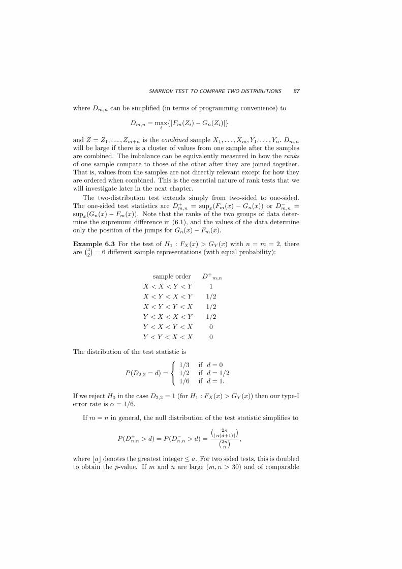
SMIRNOV TEST TO COMPARE TWO DISTRIBUTIONS 87
where Dm,n can be simplified (in terms of programming convenience) to
Dm,n = maxi|Fm(Zi)−Gn(Zi)|
and Z = Z1, . . . , Zm+n is the combined sample X1, . . . , Xm, Y1, . . . , Yn. Dm,n
will be large if there is a cluster of values from one sample after the samplesare combined. The imbalance can be equivalently measured in how the ranksof one sample compare to those of the other after they are joined together.That is, values from the samples are not directly relevant except for how theyare ordered when combined. This is the essential nature of rank tests that wewill investigate later in the next chapter.
The two-distribution test extends simply from two-sided to one-sided.The one-sided test statistics are D+
m,n = supx(Fm(x) − Gn(x)) or D−m,n =
supx(Gn(x) − Fm(x)). Note that the ranks of the two groups of data deter-mine the supremum difference in (6.1), and the values of the data determineonly the position of the jumps for Gn(x)− Fm(x).
Example 6.3 For the test of H1 : FX(x) > GY (x) with n = m = 2, thereare
(42
)= 6 different sample representations (with equal probability):
sample order D+m,n
X < X < Y < Y 1X < Y < X < Y 1/2X < Y < Y < X 1/2Y < X < X < Y 1/2Y < X < Y < X 0Y < Y < X < X 0
The distribution of the test statistic is
P (D2,2 = d) =
1/3 if d = 01/2 if d = 1/21/6 if d = 1.
If we reject H0 in the case D2,2 = 1 (for H1 : FX(x) > GY (x)) then our type-Ierror rate is α = 1/6.
If m = n in general, the null distribution of the test statistic simplifies to
P (D+n,n > d) = P (D−
n,n > d) =
(2n
bn(d+1)c)
(2nn
) ,
where bac denotes the greatest integer ≤ a. For two sided tests, this is doubledto obtain the p-value. If m and n are large (m,n > 30) and of comparable

88 GOODNESS OF FIT
Table 6.5 Tail Probabilities for Smirnov Two-Sample Test.
One-sided test α = 0.05 α = 0.025 α = 0.01 α = 0.005Two-sided test α = 0.10 α = 0.05 α = 0.02 α = 0.01
1.22q
m+nmn
1.36q
m+nmn
1.52q
m+nmn
1.63q
m+nmn
size, then an approximate distribution can be used:
P
(√mn
m + nDm,n ≤ d
)≈ 1− 2
∞∑
k=1
e−2k2d2.
A simpler large sample approximation, given in Table 6.5 works effectively ifm and n are both larger than, say, 50.
Example 6.4 Suppose we have n = m = 4 with data (x1, x2, x3, x4) =(16, 4, 7, 21) and (y1, y2, y3, y4) = (56, 31, 15, 19). For the Smirnov test ofH1 : F 6= G, the only thing important about the data is how they areranked within the group of eight combined observations:
x1:4 < x2:4 < y1:4 < x3:4 < y2:4 < x4:4 < y3:4 < y4:4.
|Fn −Gm| is never larger than 1/2, achieved in intervals (7,15), (16,19), (21,31). The p-value for the two-sided test is
p-value =2(
2×4[4×1.5]
)(84
) =2(86
)(84
) =5670
= 0.80.
Example 6.5 Figure 6.3 shows the EDFs for two samples of size 100. Oneis generated from normal data, and the other from exponential data. Theyhave identical mean (µ = 10) and variance (σ2 = 100). The MATLAB m-file
kstest and kstest2
both can be used for the two-sample test. The MATLAB code shows thep-value is 0.0018. If we compared the samples using a two-sample t-test, thesignificance value is 0.313 because the t-test is testing only the means, and notthe distribution (which is assumed to be normal). Note that supx |Fm(x) −Gn(x)| = 0.26, and according to Table 6.5, the 0.99 quantile for the two-sidedtest is 0.2305.
>> xn=randgauss(10,100,100);
>> ne=randexpo(.1,100)
>> cdfplot(xn)
>> hold on

SPECIALIZED TESTS 89
−30 −20 −10 0 10 20 30 40 500
0.1
0.2
0.3
0.4
0.5
0.6
0.7
0.8
0.9
1
F(X
)
Fig. 6.3 EDF for samples of n = m = 100 generated from normal and exponentialwith µ = 10 and σ2 = 100.
Current plot held
>> cdfplot(ne)
>> [h,p,ks2]=kstest2(xn,ne)
h = 1
p = 0.0018
ks2 = 0.2600
>> [h,p,ci]=ttest2(ne,xn)
h = 0
p = 0.3130
ci = -3.8992 1.2551
6.3 SPECIALIZED TESTS FOR GOODNESS OF FIT
In this section, we will go over some of the most important goodness-of-fittests that were made specifically for certain distributions such as the normalor exponential. In general, there is not a clear ranking on which tests beloware best and which are worst, but they all have clear advantages over theless-specific KS test.

90 GOODNESS OF FIT
Table 6.6 Null Distribution of Anderson-Darling Test Statistic: Modifications of A2
and Upper Tail Percentage Points
Upper Tail Probability αModification A∗, A∗∗ 0.10 0.05 0.025 0.01
(a) Case 0: Fully specified N (µ, σ∈) 1.933 2.492 3.070 3.857(b) Case 1: N (µ, σ∈), only σ2 known 0.894 1.087 1.285 1.551
Case 2: σ2 estimated by s2, µ known 1.743 2.308 2.898 3.702Case 3: µ and σ2 estimated, A∗ 0.631 0.752 0.873 1.035
(c) Case 4: Exp(θ), A∗∗ 1.062 1.321 1.591 1.959
6.3.1 Anderson-Darling Test
Anderson and Darling (1954) looked to improve upon the Kolmogorov-Smirnovstatistic by modifying it for distributions of interest. The Anderson-Darlingtest is used to verify if a sample of data came from a population with a specificdistribution. It is a modification of the KS test that accounts for the distri-bution and test and gives more attention to the tails. As mentioned before,the KS test is distribution free, in the sense that the critical values do notdepend on the specific distribution being tested. The Anderson-Darling testmakes use of the specific distribution in calculating the critical values. Theadvantage is that this sharpens the test, but the disadvantage is that criticalvalues must be calculated for each hypothesized distribution.
The statistics for testing H0 : F (x) = F0(x) versus the two sided alterna-tive is A2 = −n− S, where
S =n∑
i=1
2i− 1n
[log F0(Xi:n) + log(1− F0(Xn+1−i:n))] .
Tabulated values and formulas have been published (Stephens, 1974, 1976) forthe normal, lognormal, and exponential distributions. The hypothesis that thedistribution is of a specific form is rejected if the test statistic, A2 (or modifiedA∗, A∗) is greater than the critical value given in Table 6.6. Cases 0, 1, and2 do not need modification, i.e., observed A2 is directly compared to those inTable. Case 3 and (c) compare a modified A2 (A∗ or A∗∗) to the critical valuesin Table 6.6. In (b), A∗ = A2(1 + 0.75
n + 2.25n2 ), and in (c), A∗∗ = A2(1 + 0.3
n ).
Example 6.6 The following example has been used extensively in testingfor normality. The weights of 11 men (in pounds) are given: 148, 154,158, 160, 161, 162, 166, 170, 182, 195, and 236. The sample mean is 172and sample standard deviation is 24.952. Because mean and variance areestimate, this refers to Case 3 in Table 6.6. The standardized observa-tions are w1 = (148 − 172)/24.952 = −0.9618, . . . , w11 = 2.5649. and

SPECIALIZED TESTS 91
z1 = Φ(w1) = 0.1681, . . . , z11 = 0.9948. Next we calculate A2 = 0.9468 andmodify it as A∗ = A2(1 + 0.75/11 + 0.25/121) = 1.029. From the table wesee that this is significant at all levels except for α = 0.01, e.g., the null hy-pothesis of normality is rejected at level α = 0.05. Here is the correspondingMATLAB code:
>> weights = [148, 154, 158, 160, 161, 162, 166, 170, 182, 195, 236];
>> n = length(weights); ws = (weights - mean(weights))/std(weights);
>> zs = 1/2 + 1/2*erf(ws/sqrt(2));
% transformation to uniform o.s.
% calculation of anderson-darling s=0; for i = 1:n
>> s = s + (2*i-1)/n * (log(zs(i)) + log(1-zs(n+1-i)));
>> a2 = -n - s;
>> astar = a2 * (1 + 0.75/n + 2.25/n^2 );
Example 6.7 Weight is one of the most important quality characteristics ofthe positive plate in storage batteries. Each positive plate consists of a metalframe inserted in an acid-resistant bag (called ’oxide holder’) and the emptyspace in the bag is filled with active material, such as powdered lead oxide.About 75% of the weight of a positive plate consists of the filled oxide. It isalso known from past experience that variations in frame and bag weights arenegligible. The distribution of the weight of filled plate weights is, therefore,an indication of how good the filling process has been. If the process isperfectly controlled, the distribution should be normal, centered around thetarget; whereas departure from normality would indicate lack of control overthe filling operation.
Weights of 97 filled plates (chosen at random from the lot produced in ashift) are measured in grams. The data are tested for normality using theAnderson-Darling test. The data and the MATLAB program written for thispart are listed in Appendix A. The results in the MATLAB program listA2 = 0.8344 and A∗ = 0.8410.
6.3.2 Cramer-Von Mises Test
The Cramer-Von Mises test measures the weighted distance between the em-pirical CDF Fn and postulated CDF F0. Based on a squared-error function,the test statistic is
ω2n(ψ(F0)) =
∫ ∞
−∞(Fn(x)− F0(x))2 ψ(F0(x))dF0(x). (6.2)
There are several popular choices for the (weight) functional ψ. When ψ(x) =1, this is the “standard” Cramer-Von Mises statistic ω2
n(1) = ω2n, in which case

92 GOODNESS OF FIT
(a) (b)
Fig. 6.4 Harald Cramer (1893–1985); Richard von Mises (1883–1953).
the test statistic becomes
nω2n =
112n
+n∑
i=1
(F0(Xi:n)− 2i− 1
2n
)2
.
When ψ(x) = x−1(1 − x)−1, ω2n(1/(F0(1 − F0))) = A2/n, and A2 is the
Anderson-Darling statistic. Under the hypothesis H0 : F = F0, the asymp-totic distribution of ω2
n(ψ(F )) is
limn→∞
P (nω2n < x) =
1√2x
∞∑
j=0
Γ(j + 1/2)Γ(1/2)Γ(j + 1)
√4j + 1
× exp− (4j + 1)2
16x
·[J−1/4
((4j + 1)2
16x
)− J1/4
((4j + 1)2
16x
)],
where Jk(z) is the modified Bessel function (in MATLAB: bessel(k,z)).In MATLAB, the particular Cramer-Von Mises test for normality can be
applied to a sample x with the function
mtest(x, α),
where the weight function is one and α must be less than 0.10. The MATLABcode below shows how it works. Along with the simple “reject or not” output,the m-file also produces a graph (Figure 6.5) of the sample EDF along withthe N (0, 1) CDF. Note: the data are assumed to be standardized. The outputof 1 implies we do not reject the null hypothesis (H0 : N (0, 1)) at the enteredα level.

SPECIALIZED TESTS 93
−2 −1.5 −1 −0.5 0 0.5 1 1.50
0.1
0.2
0.3
0.4
0.5
0.6
0.7
0.8
0.9
1
F(X
)
−2.5 −2 −1.5 −1 −0.5 0 0.5 1 1.50
0.1
0.2
0.3
0.4
0.5
0.6
0.7
0.8
0.9
1
F(X
)
(a) (b)
Fig. 6.5 Plots of EDF versus N (0, 1) CDF for n = 25 observations of N (0, 1) dataand standardized Bin(100, 0.5) data.
>> x = rand_nor(0,1,25,1)
>> mtest(x’,0.05)
ans =
1
>> y = rand_bin(100,0.5,25)
>> y2 = (y-mean(y))/std(y)
>> mtest(y2,0.05)
ans =
1
6.3.3 Shapiro-Wilk Test for Normality
The Shapiro-Wilk (Shapiro and Wilk, 1965) test calculates a statistic thattests whether a random sample, X1, X2, . . . , Xn comes from a normal distri-bution. Because it is custom made for the normal, this test has done well incomparison studies with other goodness of fit tests (and far outperforms theKolmogorov-Smirnov test) if normally distributed data are involved.
The test statistic (W ) is calculated as
W =(∑n
i=1 aiXi:n)2∑ni=1(Xi − X)2
,
where the X1:n < X2:n < · · · < Xn:n are the ordered sample values and theai are constants generated from the means, variances and covariances of theorder statistics of a sample of size n from a normal distribution (see Table6.8). If H0 is true, W is close to one; otherwise, W < 1 and we reject H0

94 GOODNESS OF FIT
(a) (b)
Fig. 6.6 (a) Samuel S. Shapiro; (b) Martin Bradbury Wilk, born 1922.
for small values of W . Table 6.7 lists Shapiro-Wilk test statistic quantiles forsample sizes up to n = 39.
The weights ai are defined as the components of the vector
a = M ′V −1((M ′V −1)(V −1M)
)−1/2
where M denotes the expected values of standard normal order statistic for asample of size n, and V is the corresponding covariance matrix. While someof these values are tabled here, most likely you will see the test statistic (andcritical value) listed in computer output.
Example 6.8 For n = 5, the coefficients ai given in Table 6.8 lead to
W =(0.6646(x5:5 − x1:5) + 0.2413(x4:5 − x2:5))2∑
(xi − x)2.
If the data resemble a normally distributed set, then the numerator willbe approximately to
∑(xi − x)2, and W ≈ 1. Suppose (x1, . . . , x5) =
(−2,−1, 0, 1, 2), so that∑
(xi − x)2 = 10 and W = 0.1(0.6646[2 − (−2)] +0.2413[1− (−1)])2 = 0.987. From Table 6.7, w0.10 = 0.806, so our test statis-tic is clearly not significant, In fact, W ≈ w0.95 = 0.986, so the critical value(p-value) for this goodness-of-fit test is nearly 0.95. Undoubtedly the perfectsymmetry of the invented sample is a cause for this.
6.3.4 Choosing a Goodness of Fit Test
At this point, several potential goodness of fit tests have been introducedwith nary a word that recommends one over another. There are several otherspecialized tests we have not mentioned, such as the Lilliefors tests (for ex-ponentiality and normality), the D’Agostino-Pearson test, and the Bowman-Shenton test. These last two tests are extensions of the Shapiro-Wilk test.

SPECIALIZED TESTS 95
Table 6.7 Quantiles for Shapiro-Wilk Test Statistic
α
n 0.01 0.02 0.05 0.10 0.50 0.90 0.95 0.98 0.99
3 0.753 0.756 0.767 0.789 0.959 0.998 0.999 1.000 1.0004 0.687 0.707 0.748 0.792 0.935 0.987 0.992 0.996 0.9975 0.686 0.715 0.762 0.806 0.927 0.979 0.986 0.991 0.9936 0.713 0.743 0.788 0.826 0.927 0.974 0.981 0.986 0.9897 0.730 0.760 0.803 0.838 0.928 0.972 0.979 0.985 0.9888 0.749 0.778 0.818 0.851 0.932 0.972 0.978 0.984 0.9879 0.764 0.791 0.829 0.859 0.935 0.972 0.978 0.984 0.98610 0.781 0.806 0.842 0.869 0.938 0.972 0.978 0.983 0.986
11 0.792 0.817 0.850 0.876 0.940 0.973 0.979 0.984 0.98612 0.805 0.828 0.859 0.883 0.943 0.973 0.979 0.984 0.98613 0.814 0.837 0.866 0.889 0.945 0.974 0.979 0.984 0.98614 0.825 0.846 0.874 0.895 0.947 0.975 0.980 0.984 0.98615 0.835 0.855 0.881 0.901 0.950 0.975 0.980 0.984 0.987
16 0.844 0.863 0.887 0.906 0.952 0.976 0.981 0.985 0.98717 0.851 0.869 0.892 0.910 0.954 0.977 0.981 0.985 0.98718 0.858 0.874 0.897 0.914 0.956 0.978 0.982 0.986 0.98819 0.863 0.879 0.901 0.917 0.957 0.978 0.982 0.986 0.98820 0.868 0.884 0.905 0.920 0.959 0.979 0.983 0.986 0.988
21 0.873 0.888 0.908 0.923 0.960 0.980 0.983 0.987 0.98922 0.878 0.892 0.911 0.926 0.961 0.980 0.984 0.987 0.98923 0.881 0.895 0.914 0.928 0.962 0.981 0.984 0.987 0.98924 0.884 0.898 0.916 0.930 0.963 0.981 0.984 0.987 0.98925 0.888 0.901 0.918 0.931 0.964 0.981 0.985 0.988 0.989
26 0.891 0.904 0.920 0.933 0.965 0.982 0.985 0.988 0.98927 0.894 0.906 0.923 0.935 0.965 0.982 0.985 0.988 0.99028 0.896 0.908 0.924 0.936 0.966 0.982 0.985 0.988 0.99029 0.898 0.910 0.926 0.937 0.966 0.982 0.985 0.988 0.99030 0.900 0.912 0.927 0.939 0.967 0.983 0.985 0.988 0.900
31 0.902 0.914 0.929 0.940 0.967 0.983 0.986 0.988 0.99032 0.904 0.915 0.930 0.941 0.968 0.983 0.986 0.988 0.99033 0.906 0.917 0.931 0.942 0.968 0.983 0.986 0.989 0.99034 0.908 0.919 0.933 0.943 0.969 0.983 0.986 0.989 0.99035 0.910 0.920 0.934 0.944 0.969 0.984 0.986 0.989 0.990
36 0.912 0.922 0.935 0.945 0.970 0.984 0.986 0.989 0.99037 0.914 0.924 0.936 0.946 0.970 0.984 0.987 0.989 0.99038 0.916 0.925 0.938 0.947 0.971 0.984 0.987 0.989 0.99039 0.917 0.927 0.939 0.948 0.971 0.984 0.987 0.989 0.991

96 GOODNESS OF FIT
Table 6.8 Coefficients for the Shapiro-Wilk Test
n i=1 i=2 i=3 i=4 i=5 i=6 i=7 i=82 0.70713 0.7071 0.00004 0.6872 0.16775 0.6646 0.2413 0.00006 0.6431 0.2806 0.08757 0.6233 0.3031 0.1401 0.00008 0.6052 0.3164 0.1743 0.05619 0.5888 0.3244 0.1976 0.0947 0.0000
10 0.5739 0.3291 0.2141 0.2141 0.1224 0.039911 0.5601 0.3315 0.2260 0.1429 0.0695 0.000012 0.5475 0.3325 0.2347 0.1586 0.0922 0.030313 0.5359 0.3325 0.2412 0.1707 0.1099 0.0539 0.000014 0.5251 0.3318 0.2460 0.1802 0.1240 0.0727 0.024015 0.5150 0.3306 0.2495 0.1878 0.1353 0.0880 0.0433 0.000016 0.5056 0.3290 0.2521 0.1939 0.1447 0.1005 0.0593 0.0196
Obviously, the specialized tests will be more powerful than an omnibus testsuch as the Kolmogorov-Smirnov test. D’Agostino and Stephens (1986) warn
. . . for testing for normality, the Kolmogorov-Smirnov test is only a his-torical curiosity. It should never be used. It has poor power in com-parison to [specialized tests such as Shapiro-Wilk, D’Agostino-Pearson,Bowman-Shenton, and Anderson-Darling tests].
These top-performing tests fail to distinguish themselves across a broadrange of distributions and parameter values. Statistical software programsoften list two or more test results, allowing the analyst to choose the one thatwill best support their research grants.
There is another way, altogether different, for testing the fit of a distri-bution to the data. This is detailed in the upcoming section on probabilityplotting. One problem with all of the analytical tests discussed thus far in-volves the large sample behavior. As the sample size gets large, the test canafford to be pickier about what is considered a departure from the hypothe-sized null distribution F0. In short, your data might look normally distributedto you, for all practical purposes, but if it is not exactly normal, the goodnessof fit test will eventually find this out. Probability plotting is one way to avoidthis problem.

PROBABILITY PLOTTING 97
6.4 PROBABILITY PLOTTING
A probability plot is a graphical way to show goodness of fit. Althoughit is more subjective than the analytical tests (e.g., Kolmogorov-Smirnov,Anderson-Darling, Shapiro-Wilk), it has important advantages over them.First, it allows the practitioner to see what observations of the data are inagreement (or disagreement) with the hypothesized distribution. Second,while no significance level is attached to the plotted points, the analyticaltests can be misleading with large samples (this will be illustrated below).There is no such problem with large samples in probability plotting – thebigger the sample the better.
The plot is based on transforming the data with the hypothesized distribu-tion. After all, if X1, . . . , Xn have distribution F , we know F (Xi), . . . , F (Xn)are U(0, 1). Specifically, if we find a transformation with F that linearizes thedata, we can find a linear relationship to plot.
Example 6.9 Normal Distribution. If Φ represents the CDF of the stan-dard normal distribution function, then the quantile for a normal distributionwith parameters (µ, σ2) can be written as
xp = µ + Φ−1(p)σ.
The plot of xp versus Φ−1(p) is a straight line. If the line shows curvature,we know Φ−1 was not the right inverse-distribution that transformed thepercentile to the normal quantile.
A vector consisting of 1000 generated variables from N (0, 1) and 100 fromN (0.1, 1) is tested for normality. For this case, we used the Cramer-Von MisesTest using the MATLAB procedure mtest(z, α). We input a vector z of datato test, and α represents the test level. The plot in Figure 6.4(a) shows theEDF of the 1100 observations versus the best fitting normal distribution. Inthis case, the Cramer-Von Mises Test rejects the hypothesis that the dataare normally distributed at level α = 0.001. But the data are not discernablynon-normal for all practical purposes. The probability plot in Figure 6.4(b)is constructed with the MATLAB function
probplot
and confirms this conjecture.As the sample size increases, the goodness of fit tests grow increasingly
sensitive to slight perturbations in the normality assumption. In fact, theCramer-Von Mises test has correctly found the non-normality in the datathat was generated by a normal mixture.
>> [x]=randgauss(0,1,1000);
>> [y]=randgauss(0.1,1,100);
>> [z]=[x,y];

98 GOODNESS OF FIT
>> [gg]=mtest(z,.001)
gg =
0
>> probplot(z)
−2.5 −2 −1.5 −1 −0.5 0 0.5 1 1.5 2 2.50
0.1
0.2
0.3
0.4
0.5
0.6
0.7
0.8
0.9
1
F(X
)
−4 −3 −2 −1 0 1 2 3 4−4
−3
−2
−1
0
1
2
3
4
Qu
an
tile
(a) (b)
Fig. 6.7 (a) Plot of EDF vs. normal CDF, (b) normal probability plot.
Example 6.10 Thirty observations were generated from a normal distribu-tion. The MATLAB function qqweib constructs a probability plot for Weibulldata. The Weibull probability plot in Figure 6.8 shows a slight curvaturewhich suggests the model is misfit. To linearize the Weibull CDF, if the CDFis expressed as F (x) = 1− exp(−(x/γ)β), then
ln(xp) =1β
ln(− ln(1− p)) + ln(γ).
The plot of ln(xp) versus ln(− ln(1− p)) is a straight line determined by thetwo parameters β−1 and ln(γ). The MATLAB procedure qqweib also reportsthe the scale parameter scale and the shape parameter shape, estimated bythe method of least-squares.

PROBABILITY PLOTTING 99
2.05 2.1 2.15 2.2 2.25 2.3 2.35 2.4 2.45−5
−4
−3
−2
−1
0
1
2
log(data)
log
(−lo
g(1
−(i−
1/2
)/n
))
Fig. 6.8 Weibull probability plot of 30 observations generated from a normal distri-bution.
>> [x]=randgauss(10,1,30);
>> [shape,scale]=qqweib(x)
shape =
13.2094
scale =
9.9904
>>
Example 6.11 Quantile-Quantile Plots. For testing the equality oftwo distributions, the graphical analog to the Smirnov test is the Quantile-Quantile Plot, or q-q plot. The MATLAB function qqplot(x, y, ∗) plots theempirical quantiles of the vector x versus that of y. The third argument isoptional and represents the plotting symbol to use in the q-q plot. If theplotted points veer away from the 45o reference line, evidence suggests thedata are generated by populations with different distributions. Although theq-q plot leads to subjective judgment, several aspects of the distributions canbe compared graphically. For example, if the two distributions differ only bya location shift (F (x) = G(x + δ)), the plot of points will be parallel to thereference line.
Many practitioners use the q-q plot as a probability plot by replacing thesecond sample with the quantiles of the hypothesized distribution. Three

100 GOODNESS OF FIT
other MATLAB functions for probability plotting are listed below, but theyuse the q-q plot moniker. The argument symbol is optional in all three.
qqnorm(x,symbol) Normal probability plotqqweib(x,symbol) Weibull probability plotqqgamma(x,symbol) Gamma probability plot
In Figure 6.9, the q-q plots are displayed for the random generated datain the MATLAB code below. The standard qqplot MATLAB outputs (scat-terplot and dotted line fit) are enhanced by dashed line y = x representingidentity of two distributions. In each case, a distribution is plotted againstN (100, 102) data. The first case (a) represents N (120, 102) and the pointsappear parallel to the reference line because the only difference between thetwo distributions is a shift in the mean. In (b) the second distribution is dis-tributed N (100, 402). The only difference is in variance, and this is reflectedin the slope change in the plot. In the cases (c) and (d), the discrepancyis due to the lack of distribution fit; the data in (c) are generated from thet-distribution with 1 degree of freedom, so the tail behavior is much differentthan that of the normal distribution. This is evident in the left and right endof the q-q plot. In (d), the data are distributed gamma, and the illustrateddifference between the two samples is more clear.
>> x=rand_nor(100,10,30,1);
>> y1=rand_nor(120,10,30,1); qqplot(x,y1)
>> y2=rand_nor(100,40,30,1); qqplot(x,y2)
>> y3=100+10*rand_t(1,30,1); qqplot(x,y3)
>> y4=rand_gamma(200,2,30,1); qqplot(x,y4)
6.5 RUNS TEST
A chief concern in the application of statistics is to find and understand pat-terns in data apart from the randomness (noise) that obscures them. Whilehumans are good at deciphering and interpreting patterns, we are much lessable to detect randomness. For example, if you ask any large group of peo-ple to randomly choose an integer from one to ten, the numbers seven andfour are chosen nearly half the time, while the endpoints (one, ten) are rarelychosen. Someone trying to think of a random number in that range imaginessomething toward the middle, but not exactly in the middle. Anything elsejust doesn’t look “random” to us.
In this section we use statistics to look for randomness in a simple stringof dichotomous data. In many examples, the runs test will not be the mostefficient statistical tool available, but the runs test is intuitive and easier

RUNS TEST 101
90 95 100 105 110 115 120 125
90
100
110
120
130
140
80 90 100 110 120 1300
50
100
150
200
250
(a) (b)
80 90 100 110 120 130−100
0
100
200
300
400
500
600
80 90 100 110 120 13080
85
90
95
100
105
110
115
120
125
130
(c) (d)
Fig. 6.9 Data from N (100, 102) are plotted against data from (a) N (120, 102), (b)N (100, 402), (c) t1 and (d) Gamma(200, 2). The standard qqplot MATLAB outputs(scatterplot and dotted line fit) are enhanced by dashed line y = x representing identityof two distributions.

102 GOODNESS OF FIT
to interpret than more computational tests. Suppose items from the sampleX1, X2, . . . , Xn could be classified as type 1 or type 2. If the sample is random,the 1’s and 2’s are well mixed, and any clustering or pattern in 1’s and 2’s isviolating the hypothesis of randomness. To decide whether or not the patternis random, we consider the statistic R, defined as the number of homogenousruns in a sequence of ones and twos. In other words R represents the numberof times the symbols change in the sequence (including the first one). Forexample, R = 5 in this sequence of n = 11:
1 2 2 2 1 1 2 2 1 1 1.
Obviously if there were only two runs in that sequence, we could see thepattern where the symbols are separated right and left. On the other hand ifR = 11, the symbols are intermingling in a non-random way. If R is too large,the sequence is showing anti-correlation, a repulsion of same symbols, andzig-zag behavior. If R is too small, the sample is suggesting trends, clusteringand groupings in the order of the dichotomous symbols. If the null hypothesisclaims that the pattern of randomness exists, then if R is either too big ortoo small, the alternative hypothesis of an existing trend is supported.
Assume that a dichotomous sequence has n1 ones and n2 twos, n1+n2 = n.If R is the number of subsequent runs, then if the hypothesis of randomnessis true (sequence is made by random selection of 1’s and 2’s from the setcontaining n1 1’s and n2 2’s), then
fR(r) =
2(n1−1r/2−1)·(
n2−1r/2−1)
( nn1
) if r is even,
( n1−1(r−1)/2)(
n2−1(r−3)/2)+( n1−1
(r−3)/2)(n2−1
(r−1)/2)( n
n1) if r is odd,
for r = 2, 3, . . . , n. Here is a hint for solving this: first note that the numberof ways to put n objects into r groups with no cell being empty is
(n−1r−1
).
The null hypothesis is that the sequence is random, and alternatives couldbe one-sided and two sided. Also, under the hypotheses of randomness thesymbols 1 and 2 are interchangeable and without loss of generality we assumethat n1 ≤ n2. The first three central moments for R (under the hypothesis ofrandomness) are,
µR = 1 +2n1n2
n,
σR2 =
2n1n2(2n1n2 − n)n2(n− 1)
, and
E(R− µR)3 = −2n1n2(n2 − n1)2(4n1n2 − 3n)n3(n− 1)(n− 2)
,
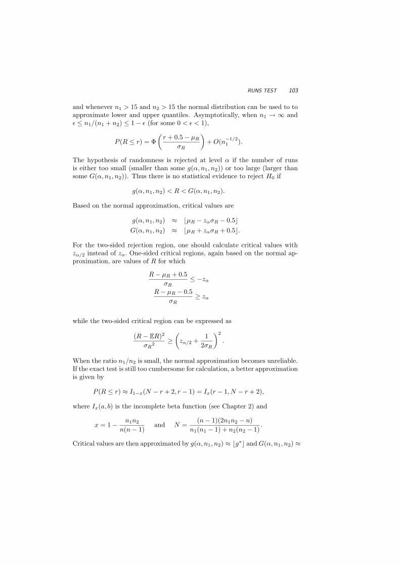
RUNS TEST 103
and whenever n1 > 15 and n2 > 15 the normal distribution can be used to toapproximate lower and upper quantiles. Asymptotically, when n1 → ∞ andε ≤ n1/(n1 + n2) ≤ 1− ε (for some 0 < ε < 1),
P (R ≤ r) = Φ(
r + 0.5− µR
σR
)+ O(n−1/2
1 ).
The hypothesis of randomness is rejected at level α if the number of runsis either too small (smaller than some g(α, n1, n2)) or too large (larger thansome G(α, n1, n2)). Thus there is no statistical evidence to reject H0 if
g(α, n1, n2) < R < G(α, n1, n2).
Based on the normal approximation, critical values are
g(α, n1, n2) ≈ bµR − zασR − 0.5cG(α, n1, n2) ≈ bµR + zασR + 0.5c.
For the two-sided rejection region, one should calculate critical values withzα/2 instead of zα. One-sided critical regions, again based on the normal ap-proximation, are values of R for which
R− µR + 0.5σR
≤ −zα
R− µR − 0.5σR
≥ zα
while the two-sided critical region can be expressed as
(R− ER)2
σR2
≥(
zα/2 +1
2σR
)2
.
When the ratio n1/n2 is small, the normal approximation becomes unreliable.If the exact test is still too cumbersome for calculation, a better approximationis given by
P (R ≤ r) ≈ I1−x(N − r + 2, r − 1) = Ix(r − 1, N − r + 2),
where Ix(a, b) is the incomplete beta function (see Chapter 2) and
x = 1− n1n2
n(n− 1)and N =
(n− 1)(2n1n2 − n)n1(n1 − 1) + n2(n2 − 1)
.
Critical values are then approximated by g(α, n1, n2) ≈ bg∗c and G(α, n1, n2) ≈

104 GOODNESS OF FIT
1 + bG∗c, where g∗ and G∗ are solutions to
I1−x(N − g∗ + 2, g∗ − 1) = α,
Ix(G∗ − 1, N −G∗ + 3) = α.
Example 6.12 The tourism officials in Santa Cruz worried about globalworming and El Nino effect, compared daily temperatures (7/1/2003 - 7/21/2003)with averages of corresponding daily temperatures in 1993-2002. If the tem-perature in year 2003 is above the same day average in 1993-2002, then symbolA is recorded, if it is below, the symbol B is recorded. The following sequenceof 21 letters was obtained:
AAABBAA|AABAABA|AAABBBB.
We wish to test the hypothesis of random direction of deviation from theaverage temperature against the alternative of non-randomness at level α =5%. The MATLAB procedure for computing the test is runs test.
>> cruz = [1 1 1 2 2 1 1 1 1 2 1 1 2 1 1 1 1 2 2 2 2];
>> [problow, probup, nruns, expectedruns] = runs_test(cruz)
runones = 4
runtwos = 4
trun = 8
n1 = 13
n2 = 8
n = 21
problow = 0.1278
probup = 0.0420
nruns = 8
expectedruns = 10.9048
If observed number of runs is LESS than expected, problow is
P (R = 2) + · · ·+ P (R = nruns)
and probup is
P (R = n− nruns + 2) + · · ·+ P (R = n).
Alternatively, if nruns is LARGER than expected, then problow is
P (R = 2) + · · ·+ P (R = n− nruns + 2)
and probup is
P (R = nruns) + · · ·+ P (R = n).
In this case, the number of runs (8) was less than expected (10.9048), and theprobability of seeing 8 or fewer runs in a random scattering is 0.1278. But this

RUNS TEST 105
0
0.05
0.1
0.15
0.2
2 3 4 5 6 7 8 9 10 11 12 13 14 15 16 17
R
P(R
)
Fig. 6.10 Probability distribution of runs under H0.
is a two-sided test. This MATLAB test implies we should use P (R ≥ n−n2+2)= P (R ≥ 15) = 0.0420 as the “other tail” to include in the critical region(which would make the p-value equal to 0.1698). But using P (R ≥ 15) isslightly misleading, because there is no symmetry in the null distribution ofR; instead, we suggest using 2*problow = 0.2556 as the critical value for atwo-sided test.
Example 6.13 The following are 30 time lapses, measured in minutes, be-tween eruptions of Old Faithful geyser in Yellowstone National Park. In theMATLAB code below, forruns stores 2 if the temperature is below aver-age, otherwise stores 1. The expected number of runs (15.9333) is largerthan what was observed (13), and the p-value for the two-sided runs test is2*0.1678=0.3356.
>> oldfaithful = [68 63 66 63 61 44 60 62 71 62 62 55 62 67 73 ...
72 55 67 68 65 60 61 71 60 68 67 72 69 65 66];
>> mean(oldfaithful)
ans = 64.1667
>> forruns = (oldfaithful - 64.1667 > 0) + 1
forruns =
2 1 2 1 1 1 1 1 2 1
1 1 1 2 2 2 1 2 2 2
1 1 2 1 2 2 2 2 2 2
>> [problow, probup, nruns, expectedruns] = runs_test(forruns)

106 GOODNESS OF FIT
runones = 6
runtwos = 7
trun = 13
n1 = 14
n2 = 16
n = 30
problow = 0.1804
probup = 0.1678
nruns = 13
expectedruns = 15.9333
Before we finish with the runs test, we are compelled to make note of itslimitations. After its inception by Mood (1940), the runs test was used asa cure-all nonparametric procedure for a variety of problems, including two-sample comparisons. However, it is inferior to more modern tests we willdiscuss in Chapter 7. More recently, Mogull (1994) showed an anomaly of theone-sample runs test; it is unable to reject the null hypothesis for series ofdata with run length of two.
6.6 META ANALYSIS
Meta analysis is concerned with combining the inference from several studiesperformed under similar conditions and experimental design. From each studyan “effect size” is derived before the effects are combined and their variabilityassessed. However, for optimal meta analysis, the analyst needs substantialinformation about the experiment such as sample sizes, values of the teststatistics, the sampling scheme and the test design. Such information is oftennot provided in the published work. In many cases, only the p-values ofparticular studies are available to be combined.
Meta analysis based on p-values only is often called nonparametric or om-nibus meta analysis because the combined inference dose not depend on theform of data, test statistics, or distributions of the test statistics. There aremany situations in which such combination of tests is needed. For example,one might be interested in
(i) multiple t tests in testing equality of two treatments versus one sidedalternative. Such tests often arise in function testing and estimation,fMRI, DNA comparison, etc;
(ii) multiple F tests for equality of several treatment means. The testmay not involve the same treatments and parametric meta analysis maynot be appropriate; or
(iii) multiple χ2 tests for testing the independence in contingency tables(see Chapter 9). The table counts may not be given or the tables couldbe of different size (the same factor of interest could be given at differentlevels).
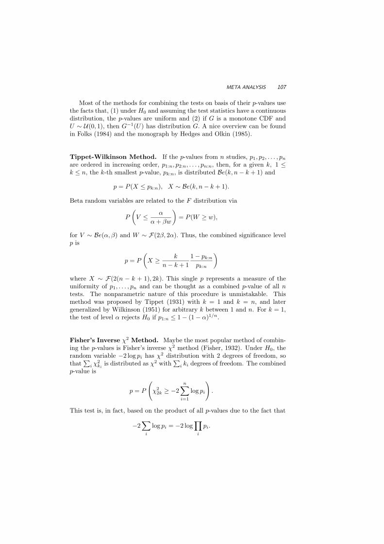
META ANALYSIS 107
Most of the methods for combining the tests on basis of their p-values usethe facts that, (1) under H0 and assuming the test statistics have a continuousdistribution, the p-values are uniform and (2) if G is a monotone CDF andU ∼ U(0, 1), then G−1(U) has distribution G. A nice overview can be foundin Folks (1984) and the monograph by Hedges and Olkin (1985).
Tippet-Wilkinson Method. If the p-values from n studies, p1, p2, . . . , pn
are ordered in increasing order, p1:n, p2:n, . . . , pn:n, then, for a given k, 1 ≤k ≤ n, the k-th smallest p-value, pk:n, is distributed Be(k, n− k + 1) and
p = P (X ≤ pk:n), X ∼ Be(k, n− k + 1).
Beta random variables are related to the F distribution via
P
(V ≤ α
α + βw
)= P (W ≥ w),
for V ∼ Be(α, β) and W ∼ F(2β, 2α). Thus, the combined significance levelp is
p = P
(X ≥ k
n− k + 11− pk:n
pk:n
)
where X ∼ F(2(n − k + 1), 2k). This single p represents a measure of theuniformity of p1, . . . , pn and can be thought as a combined p-value of all ntests. The nonparametric nature of this procedure is unmistakable. Thismethod was proposed by Tippet (1931) with k = 1 and k = n, and latergeneralized by Wilkinson (1951) for arbitrary k between 1 and n. For k = 1,the test of level α rejects H0 if p1:n ≤ 1− (1− α)1/n.
Fisher’s Inverse χ2 Method. Maybe the most popular method of combin-ing the p-values is Fisher’s inverse χ2 method (Fisher, 1932). Under H0, therandom variable −2 log pi has χ2 distribution with 2 degrees of freedom, sothat
∑i χ2
kiis distributed as χ2 with
∑i ki degrees of freedom. The combined
p-value is
p = P
(χ2
2k ≥ −2n∑
i=1
log pi
).
This test is, in fact, based on the product of all p-values due to the fact that
−2∑
i
log pi = −2 log∏
i
pi.

108 GOODNESS OF FIT
Averaging p-Values by Inverse Normals. The following method forcombining p-values is based on the fact that if Z1, Z2, . . . , Zn are i.i.d. N (0, 1),then (Z1 + Z2 + · · ·+ Zn)/
√n is distributed N (0, 1), as well. Let Φ−1 denote
the inverse function to the standard normal CDF Φ, and let p1, p2, . . . , pn bethe p-values to be averaged. Then the averaged p-value is
p = P
(Z >
Φ−1(1− p1) + . . . Φ−1(1− pn)√n
),
where Z ∼ N (0, 1). This procedure can be extended by using weighted sums:
p = P
(Z >
λ1Φ−1(1− p1) + · · ·+ λnΦ−1(1− pn)√λ2
1 + · · ·+ λ2n
).
There are several more approaches in combining the p-values. Good (1955)suggested use of weighted product
−2∑
i
log pi = −2 log∏
i
pλii ,
but the distributional theory behind this statistic is complex. Mudholkar andGeorge (1979) suggest transforming the p-values into logits, that is, logit(p) =log(p/(1− p)). The combined p-value is
p ≈ P
(t5n+4 >
−∑ni=1 logit(pi)√
π2n/3
).
As an alternative, Lancaster (1961) proposes a method based on inversegamma distributions.
Example 6.14 This example is adapted from a presentation by Jessica Uttsfrom University of California, Davis. Two scientists, Professors A and B,each have a theory they would like to demonstrate. Each plans to run a fixednumber of Bernoulli trials and then test H0 : p = 0.25 verses H1 : p > 0.25.
Professor A has access to large numbers of students each semester to useas subjects. He runs the first experiment with 100 subjects, and there are33 successes (p = 0.04). Knowing the importance of replication, Professor Athen runs an additional experiment with 100 subjects. He finds 36 successes(p = 0.009).
Professor B only teaches small classes. Each quarter, she runs an experi-ment on her students to test her theory. Results of her ten studies are givenin the table below.
At first glance professor A’s theory has much stronger support. After all,the p-values are 0.04 and 0.009. None of the ten experiments of professor

EXERCISES 109
B was found significant. However, if the results of the experiment for eachprofessor are aggregated, Professor B actually demonstrated a higher level ofsuccess than Professor A, with 71 out of 200 as opposed to 69 out of 200successful trials. The p-values for the combined trials are 0.0017 for ProfessorA and 0.0006 for Professor B.
n # of successes p-value
10 4 0.2215 6 0.1517 6 0.2325 8 0.1730 10 0.2040 13 0.1818 7 0.1410 5 0.0815 5 0.3120 7 0.21
Now suppose that reports of the studies have been incomplete and onlyp-values are supplied. Nonparametric meta analysis performed on 10 studiesof Professor B reveals an overall omnibus test significant. The MATLAB codefor Fisher’s and inverse-normal methods are below; the combined p-values forProfessor B are 0.0235 and 0.021.
>> pvals = [0.22, 0.15, 0.23, 0.17, 0.20, 0.18, 0.14, 0.08, 0.31, 0.21];
>> fisherstat = - 2 * sum( log(pvals))
fisherstat =
34.4016
>> 1-chi2cdf(fisherstat, 2*10)
ans =
0.0235
>> 1 - normcdf( sum(norminv(1-pvals))/sqrt(length(pvals)) )
ans =
0.0021
6.7 EXERCISES
6.1. Derive the exact distribution of the Kolmogorov test statistic Dn for thecase n = 1.
6.2. Go the NIST link below to download 31 measurements of polished win-dow strength data for a glass airplane window. In reliability tests suchas this one, researchers rely on parametric distributions to character-ize the observed lifetimes, but the normal distribution is not commonly

110 GOODNESS OF FIT
used. Does this data follow any well-known distribution? Use probabil-ity plotting to make your point.
http://www.itl.nist.gov/div898/handbook/eda/section4/eda4291.htm
6.3. Go to the NIST link below to download 100 measurements of the speedof light in air. This classic experiment was carried out by a U.S. NavalAcademy teacher Albert Michelson is 1879. Do the data appear to benormally distributed? Use three tests (Kolmogorov, Anderson-Darling,Shapiro-Wilk) and compare answers.
http://www.itl.nist.gov/div898/strd/univ/data/Michelso.dat
6.4. Do those little peanut bags handed out during airline flights actuallycontain as many peanuts as they claim? From a box of peanut bagsthat have 14g label weights, fifteen bags are sampled and weighed: 16.4,14.4, 15.5, 14.7, 15.6, 15.2, 15.2, 15.2, 15.3, 15.4, 14.6, 15.6, 14.7, 15.9,13.9. Are the data approximately normal so that a t-test has validity?
6.5. Generate a sample S0 of size m = 47 from the population with normalN (3, 1) distribution. Test the hypothesis that the sample is standardnormal H0 : F = F0 = N (0, 1) (not at µ = 3) versus the alternativeH1 : F < F0. You will need to use D−
n in the test. Repeat this testingprocedure (with new samples, of course) 1000 times. What proportionof p-values exceeded 5%?
6.6. Generate two samples of sizes m = 30 and m = 40 from U(0, 1). Squarethe observations in the second sample. What is the theoretical distri-bution of the squared uniforms? Next, “forget” that you squared thesecond sample and test by Smirnov test equality of the distributions.Repeat this testing procedure (with new samples, of course) 1000 times.What proportion of p-values exceeded 5%?
6.7. In MATLAB, generate two data sets of size n = 10, 000: the first fromN (0, 1) and the second from the t distribution with 5 degrees of free-dom. These are your two samples to be tested for normality. Recall theasymptotic properties of order statistics from Chapter 5 and find theapproximate distribution of X[3000]. Standardize it appropriately (herep = 0.3, and µ = norminv(0.3) = −0.5244, and find the two-sidedp-values for the goodness-of-fit test of the normal distribution. If thetesting is repeated 10 times, how many times will you reject the hy-pothesis of normality for the second, t distributed sequence? What ifthe degrees of freedom in the t sequence increase from 5 to 10; to 40?Comment.
6.8. For two samples of size m = 2 and n = 4, find the exact distributionof the Smirnov test statistics for the test of H0 : F (x) ≤ G(x) versusH1 : F (x) > G(x).

EXERCISES 111
6.9. Let X1, X2, . . . , Xn1 be a sample from a population with distribution FX
and Y1, Y2, . . . , Yn2 be a sample from distribution FY . If we are interestedin testing H0 : FX = FY one possibility is to use the runs test in thefollowing way. Combine the two samples and let Z1, Z2, . . . , Zn1+n2
denote the respective order statistics. Let dichotomous variables 1 and2 signify if Z is from the first or the second sample. Generate 50 U(0,1)numbers and 50 N (0,1) numbers. Concatenate and sort them. Keeptrack of each number’s source by assigning 1 if the number came fromthe uniform distribution and 2 otherwise. Test the hypothesis that thedistributions are the same.
6.10. Combine the p-values for Professor B from the meta-analysis exampleusing the Tippet-Wilkinson method with the smallest p-value and Lan-caster’s Method.
6.11. Derive the exact distribution of the number of runs for n = 4 when thereare n1 = n2 = 2 observations of ones and twos. Base your derivation onthe exhausting all
(42
)possible outcomes.
6.12. The link below connects you to the Dow-Jones Industrial Average (DJIA)closing values from 1900 to 1993. First column contains the date (yym-mdd), second column contains the value. Use the runs test to see if thereis a non-random pattern in the increases and decreases in the sequenceof closing values. Consult
http://lib.stat.cmu.edu/datasets/djdc0093
6.13. Recall Exercise 5.1. Repeat the simulation and make a comparisonbetween the two populations using qqplot. Because the sample rangehas a beta Be(49, 2). distribution, this should be verified with a straightline in the plot.
6.14. The table below displays the accuracy of meteorological forecasts forthe city of Marietta, Georgia. Results are supplied for the month ofFebruary, 2005. If the forecast differed for the real temperature formore than 3F , the symbol 1 was assigned. If the forecast was in errorlimits < 3F , the symbol 2 was assigned. Is it possible to claim thatcorrect and wrong forecasts group at random?
2 2 2 2 2 2 2 2 2 2 2 1 1 11 1 2 2 1 1 2 2 2 2 2 1 2 2
6.15. Previous records have indicated that the total points of Olympic divesare normally distributed. Here are the records for Men 10-meter Plat-form Preliminary in 2004. Test the normality of the point distribution.For a computational exercise, generate 1000 sets of 33 normal obser-vations with the same mean and variance as the diving point data.

112 GOODNESS OF FIT
Use the Smirnov test to see how often the p-value corresponding tothe test of equal distributions exceeds 0.05. Comment on your results.Rank Name Country Points Lag
1 HELM, Mathew AUS 513.062 DESPATIE, Alexandre CAN 500.55 12.513 TIAN, Liang CHN 481.47 31.594 WATERFIELD, Peter GBR 474.03 39.035 PACHECO, Rommel MEX 463.47 49.596 HU, Jia CHN 463.44 49.627 NEWBERY, Robert AUS 461.91 51.158 DOBROSKOK, Dmitry RUS 445.68 67.389 MEYER, Heiko GER 440.85 72.2110 URAN-SALAZAR, Juan G. COL 439.77 73.2911 TAYLOR, Leon GBR 433.38 79.6812 KALEC, Christopher CAN 429.72 83.3413 GALPERIN, Gleb RUS 427.68 85.3814 DELL’UOMO, Francesco ITA 426.12 86.9415 ZAKHAROV, Anton UKR 420.3 92.7616 CHOE, Hyong Gil PRK 419.58 93.4817 PAK, Yong Ryong PRK 414.33 98.7318 ADAM, Tony GER 411.3 101.7619 BRYAN, Nickson MAS 407.13 105.9320 MAZZUCCHI, Massimiliano ITA 405.18 107.8821 VOLODKOV, Roman UKR 403.59 109.4722 GAVRIILIDIS, Ioannis GRE 395.34 117.7223 GARCIA, Caesar USA 388.77 124.2924 DURAN, Cassius BRA 387.75 125.3125 GUERRA-OLIVA, Jose Antonio CUB 375.87 137.1926 TRAKAS, Sotirios GRE 361.56 151.527 VARLAMOV, Aliaksandr BLR 361.41 151.6528 FORNARIS, ALVAREZ Erick CUB 351.75 161.3129 PRANDI, Kyle USA 346.53 166.5330 MAMONTOV, Andrei BLR 338.55 174.5131 DELALOYE, Jean Romain SUI 326.82 186.2432 PARISI, Hugo BRA 325.08 187.9833 HAJNAL, Andras HUN 305.79 207.27
6.16. Consider the Cramer von Mises test statistic with ψ(x) = 1. With asample of n = 1, derive the test statistic distribution and show that itis maximized at X = 1/2.
6.17. Generate two samples S1 and S2, of sizes m = 30 and m = 40 fromthe uniform distribution. Square the observations in the second sam-ple. What is the theoretical distribution of the squared uniforms? Next,“forget” that you squared the second sample and test equality of the dis-tributions. Repeat this testing procedure (with new samples, of course)1000 times. What proportion of p-values exceeded 5%?

REFERENCES 113
6.18. Recall the Gumbel distribution (or extreme value distribution) fromChapter 5. Linearize the CDF of the Gumbel distribution to show howa probability plot could be constructed.
REFERENCES
Anderson, T. W., and Darling, D. A. (1954), “A Test of Goodness of Fit,”Journal of the American Statistical Association, 49, 765-769.
Birnbaum, Z. W., and Tingey, F. (1951), “One-sided Confidence Contours forProbability Distribution Functions,” Annals of Mathematical Statistics,22, 592-596.
D’Agostino, R. B., and Stephens, M. A. (1986), Goodness-of-Fit Techniques,New York: Marcel Dekker.
Feller, W. (1948), On the Kolmogorov-Smirnov Theorems, Annals of Mathe-matical Statistics, 19, 177-189.
Fisher, R. A. (1932), Statistical Methods for Research Workers, 4th ed, Edin-burgh, UK: Oliver and Boyd.
Folks, J. L. (1984), “Combination of Independent Tests,” in Handbook ofStatistics 4, Nonparametric Methods, Eds. P. R. Krishnaiah and P. K.Sen, Amsterdam, North-Holland: Elsevier Science, pp. 113-121.
Good, I. J. (1955), “On the Weighted Combination of Significance Tests,”Journal of the Royal Statistical Society (B), 17, 264265.
Hedges, L. V., and Olkin, I. (1985), Statistical Methods for Meta-Analysis,New York: Academic Press.
Kolmogorov, A. N. (1933), “Sulla Determinazione Empirica di Una Legge diDistribuzione,” Giornio Instituto Italia Attuari, 4, 83-91.
Lancaster, H. O. (1961), “The Combination of Probabilities: An Applicationof Orthonormal Functions,” Australian Journal of Statistics,3, 20-33.
Miller, L. H. (1956), “Table of percentage points of Kolmogorov Statistics,”Journal of the American Statistical Association, 51, 111-121.
Mogull, R. G. (1994). “The one-sample runs test: A category of exception,”Journal of Educational and Behavioral Statistics 19, 296-303.
Mood, A. (1940), “The distribution theory of runs,” Annals of MathematicalStatistics, 11, 367–392.
Mudholkar, G. S., and George, E. O. (1979), “The Logit Method for Combin-ing Probabilities,” in Symposium on Optimizing Methods in Statistics,ed. J. Rustagi, New York: Academic Press, pp. 345-366.
Pearson, K. (1902), “On the Systematic Fitting of Curves to Observationsand Measurements,” Biometrika, 1, 265-303.

114 GOODNESS OF FIT
Roeder, K. (1990), “Density Estimation with Confidence Sets Exemplifiedby Superclusters and Voids in the Galaxies,” Journal of the AmericanStatistical Association, 85, 617-624.
Shapiro, S. S., and Wilk, M. B. (1965), “An Analysis of Variance Test forNormality (Complete Samples),” Biometrika, 52, 591-611.
Smirnov, N. V. (1939a), “On the Derivations of the Empirical DistributionCurve,” Matematicheskii Sbornik, 6, 2-26.
(1939b), “On the Estimation of the Discrepancy Between EmpiricalCurves of Distribution for Two Independent Samples,” Bulletin MoscowUniversity, 2, 3-16.
Stephens, M. A. (1974), “EDF Statistics for Goodness of Fit and Some Com-parisons,” Journal of the American Statistical Association,69, 730-737.
(1976), “Asymptotic Results for Goodness-of-Fit Statistics with Un-known Parameters,” Annals of Statistics, 4, 357-369.
Tippett, L. H. C. (1931), The Method of Statistics, 1st ed., London: Williamsand Norgate.
Wilkinson, B. (1951), “A Statistical Consideration in Psychological Research,”Psychological Bulletin, 48, 156-158.

7Rank Tests
Each of us has been doing statistics all his life, in the sense that each ofus has been busily reaching conclusions based on empirical observationsever since birth.
William Kruskal
All those old basic statistical procedures – the t-test, the correlation coeffi-cient, the analysis of variance (ANOVA) – depend strongly on the assumptionthat the sampled data (or the sufficient statistics) are distributed according toa well-known distribution. Hardly the fodder for a nonparametrics text book.But for every classical test, there is a nonparametric alternative that does thesame job with fewer assumptions made of the data. Even if the assumptionsfrom a parametric model are modest and relatively non-constraining, theywill undoubtedly be false in the most pure sense. Life, along with your ex-perimental data, are too complicated to fit perfectly into a framework of i.i.d.errors and exact normal distributions.
Mathematicians have been researching ranks and order statistics since agesago, but it wasn’t until the 1940s that the idea of rank tests gained prominencein the statistics literature. Hotelling and Pabst (1936) wrote one of the firstpapers on the subject, focusing on rank correlations.
There are nonparametric procedures for one sample, for comparing twoor more samples, matched samples, bivariate correlation, and more. Thekey to evaluating data in a nonparametric framework is to compare obser-vations based on their ranks within the sample rather than entrusting the
115

116 RANK TESTS
(a) (b) (c)
Fig. 7.1 Frank Wilcoxon (1892–1965), Henry Berthold Mann (1905–2000), and Pro-fessor Emeritus Donald Ransom Whitney
actual data measurements to your analytical verdicts. The following tableshows non-parametric counterparts to the well known parametric procedures(WSiRT/WSuRT stands for Wilcoxon Signed/Sum Rank Test).
PARAMETRIC NON-PARAMETRIC
Pearson coefficient of correlation Spearman coefficient of correlationOne sample t-test for the location sign test, WSiRT
paired test t test sign test, WSiRTtwo sample t test WSurT, Mann-Whitney
ANOVA Kruskal-Wallis TestBlock Design ANOVA Friedman Test
To be fair, it should be said that many of these nonparametric procedurescome with their own set of assumptions. We will see, in fact, that some ofthem are rather obtrusive on an experimental design. Others are much lessso. Keep this in mind when a nonparametric test is touted as “assumptionfree”. Nothing in life is free.
In addition to properties of ranks and basic sign test, in this chapter wewill present the following nonparametric procedures:
• Spearman Coefficient: Two-sample correlation statistic.
• Wilcoxon Test: One-sample median test (also see Sign Test).
• Wilcoxon Sum Rank Test: Two-sample test of distributions.
• Mann-Whitney Test: Two-sample test of medians.
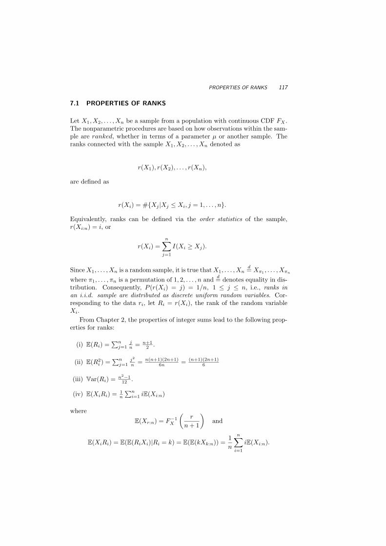
PROPERTIES OF RANKS 117
7.1 PROPERTIES OF RANKS
Let X1, X2, . . . , Xn be a sample from a population with continuous CDF FX .The nonparametric procedures are based on how observations within the sam-ple are ranked, whether in terms of a parameter µ or another sample. Theranks connected with the sample X1, X2, . . . , Xn denoted as
r(X1), r(X2), . . . , r(Xn),
are defined as
r(Xi) = #Xj |Xj ≤ Xi, j = 1, . . . , n.
Equivalently, ranks can be defined via the order statistics of the sample,r(Xi:n) = i, or
r(Xi) =n∑
j=1
I(Xi ≥ Xj).
Since X1, . . . , Xn is a random sample, it is true that X1, . . . , Xnd= Xπ1 , . . . , Xπn
where π1, . . . , πn is a permutation of 1, 2, . . . , n and d= denotes equality in dis-tribution. Consequently, P (r(Xi) = j) = 1/n, 1 ≤ j ≤ n, i.e., ranks inan i.i.d. sample are distributed as discrete uniform random variables. Cor-responding to the data ri, let Ri = r(Xi), the rank of the random variableXi.
From Chapter 2, the properties of integer sums lead to the following prop-erties for ranks:
(i) E(Ri) =∑n
j=1jn = n+1
2 .
(ii) E(R2i ) =
∑nj=1
j2
n = n(n+1)(2n+1)6n = (n+1)(2n+1)
6
(iii) Var(Ri) = n2−112 .
(iv) E(XiRi) = 1n
∑ni=1 iE(Xi:n)
where
E(Xr:n) = F−1X
(r
n + 1
)and
E(XiRi) = E(E(RiXi)|Ri = k) = E(E(kXk:n)) =1n
n∑
i=1
iE(Xi:n).

118 RANK TESTS
In the case of ties, it is customary to average the tied rank values. TheMATLAB procedure rank does just that:
>> ranks([3 1 4 1 5 9 2 6 5 3 5 8 9])
ans =
Columns 1 through 7
4.5000 1.5000 6.0000 1.5000 8.0000 12.5000 3.0000
Columns 8 through 13
10.0000 8.0000 4.5000 8.0000 11.0000 12.5000
Property (iv) can be used to find the correlation between observations andtheir ranks. Such correlation depends on the sample size and the underlyingdistribution. For example, for X ∼ U(0, 1), E(XiRi) = (2n + 1)/6, whichgives Cov(Xi, Ri) = (n− 1)/12 and Corr(Xi, Ri) =
√(n− 1)/(n + 1).
With two samples, comparisons between populations can be made in anonparametric way by comparing ranks for the combined ordered samples.Rank statistics that are made up of sums of indicator variables comparingitems from one sample with those of the other are called linear rank statistics.
7.2 SIGN TEST
Suppose we are interested in testing the hypothesis H0 that a population withcontinuous CDF has a median m0 against one of the alternatives H1 : m > m0,H1 : m < m0 or H1 : m 6= m0. Designate the sign + when Xi > m0 (i.e., whenthe difference Xi −m0 is positive), and the sign − otherwise. For continuousdistributions, the case Xi = m (a tie) is theoretically impossible, although inpractice ties are often possible, and this feature can be accommodated. Fornow, we assume the ideal situation in which the ties are not present.
Assumptions: Actually, no assumptions are necessary for the sign testother than the data are at least ordinal
If m0 is the median, i.e., if H0 is true, then by definition of the median,P (Xi > m0) = P (Xi < m0) = 1/2. If we let T be the total number of +signs, that is,
T =n∑
i=1
I(Xi > m0),
then T ∼ Bin(n, 1/2).Let the level of test, α, be specified. When the alternative is H1 : m > m0,
the critical values of T are integers larger than or equal to tα, which is definedas the smallest integer for which

SIGN TEST 119
P (T ≥ tα|H0) =n∑
t=tα
(n
t
)(12
)n
< α.
Likewise, if the alternative is H1 : m < m0, the critical values of T are integerssmaller than or equal to t′α, which is defined as the largest integer for which
P (T ≤ t′α|H0) =t′α∑
t=0
(n
t
)(12
)n
< α.
If the alternative hypothesis is two-sided (H1 : m 6= m0), the critical valuesof T are integers smaller than or equal to t′α/2 and integers larger than or equalto tα/2, which are defined via
t′α/2∑t=0
(n
t
)(12
)n
< α/2, andn∑
t=tα/2
(n
t
)(12
)n
< α/2.
If the value T is observed, then in testing against alternative H1 : m > m0,large values of T serve as evidence against H0 and the p-value is
p =n∑
i=T
(n
i
)2−n =
n−T∑
i=0
(n
i
)2−n.
When testing against the alternative H1 : m < m0, small values of T arecritical and the p-value is
p =T∑
i=0
(n
i
)2−n.
When the hypothesis is the two-sided, take T ′ = minT, n−T and calculatep-value as
p = 2T ′∑
i=0
(n
i
)2−n.
7.2.1 Paired Samples
Consider now the case in which two samples are paired:
(X1, Y1), . . . , (Xn, Yn).
Suppose we are interested in finding out whether the median of the populationdifferences is 0. In this case we let T =
∑ni=1 I(Xi > Yi), which is the total
number of strictly positive differences.

120 RANK TESTS
For two population means it is true that the hypothesis of equality of meansis equivalent to the hypothesis that the mean of the population differences isequal to zero. This is not always true for the test of medians. That is, ifD = X − Y , then it is quite possible that mD 6= mX − mY . With the signtest we are not testing the equality of two medians, but whether the medianof the difference is 0.
Under H0: equal population medians, E(T ) =∑
P (Xi > Yi) = n/2 andVar(T ) = n ·Var(I(X > Y )) = n/4. With large enough n, T is approximatelynormal, so for the statistical test of H1: the medians are not equal, we wouldreject H0 if T is far enough away from n/2; that is,
z0 =T − n/2√
n/2: reject H0 if |z0| > zα/2.
Example 7.1 According to The Rothstein Catalog on Disaster Recovery,the median number of violent crimes per state dropped from the year 1999to 2000. Of 50 states, if Xi is number of violent crimes in state i in 1999and Yi is the number for 2000, the median of sample differences is Xi − Yi.This number decreased in 38 out of 50 states in one year. With T = 38 andn = 50, we find z0 = 3.67, which has a p-value of 0.00012 for the one-sidedtest (medians decreased over the year) or .00024 for the two-sided test.
Example 7.2 Let X1 and X2 be independent random variables distributedas Poisson with parameters λ1 and λ2. We would like to test the hypothesisH0 : λ1 = λ2 (= λ). If H0 is true,
P (X1 = k, X2 = l) =(2λ)k+l
(k + l)!e−2λ
(k + l
k
) (12
)k+l
.
If we observe X1 and X2 and if X1 + X2 = n then testing H0 is exactly thesign test, with T = X1. Indeed,
P (X1 = k | X1 + X2 = n) =(
n
k
) (12
)n
.
For instance, if X1 = 10 and X2 = 20 are observed, then the p-value for thetwo-sided alternative H1 : λ1 6= λ2 is 2
∑10i=0
(30i
) (12
)30 = 2 · 0.0494 = 0.0987.
Example 7.3 Hogmanay Celebration1 Roger van Gompel and Shona Fal-coner at the University of Dundee conducted an experiment to examine the
1Hogmanay is the Scottish New Year, celebrated on 31st December every year. The nightinvolves a celebratory drink or two, fireworks and kissing complete strangers (not necessarilyin that order).

SIGN TEST 121
drinking patterns of Members of the Scottish Parliament over the festive hol-iday season.
Being elected to the Scottish Parliament is likely to have created in mem-bers a sense of stereotypical conformity so that they appear to fit in with thetraditional ways of Scotland, pleasing the tabloid newspapers and ensuringpopular support. One stereotype of the Scottish people is that they drink alot of whisky, and that they enjoy celebrating both Christmas and Hogmanay.However, it is possible that members of parliment tend to drink more whiskyat one of these times compared to the other, and an investigation into thiswas carried out.
The measure used to investigate any such bias was the number of unitsof single malt scotch whisky (“drams”) consumed over two 48-hour periods:Christmas Eve/Christmas Day and Hogmanay/New Year’s Day. The hypoth-esis is that Members of the Scottish Parliament drink a significantly differentamount of whisky over Christmas than over Hogmanay (either consistentlymore or consistently less). The following data were collected.
MSP 1 2 3 4 5 6 7 8 9
Drams at Christmas 2 3 3 2 4 0 3 6 2Drams at Hogmanay 5 1 5 6 4 7 5 9 0
MSP 10 11 12 13 14 15 16 17 18
Drams at Christmas 2 5 4 3 6 0 3 3 0Drams at Hogmanay 4 15 6 8 9 0 6 5 12
The MATLAB function sign test1 lists five summary statistics from thedata for the sign test. The first is a p-value based on randomly assigning a’+’ or ’–’ to tied values (see next subsection), and the second is the p-valuebased on the normal approximation, where ties are counted as half. n is thenumber of non-tied observations, plus are the number of plusses in y−x, andtie is the number of tied observations.
>> x=[2 3 3 2 4 0 3 6 2 2 5 4 3 6 0 3 3 0];
>> y=[5 1 5 6 4 7 5 9 0 4 15 6 8 9 0 6 5 12];
>> [p1 p2 n plus tie] = sign_test1(x’,y’)
p1 =
0.0021
p2 =
0.0030
n =
16

122 RANK TESTS
plus =
2
tie =
2
7.2.2 Treatments of Ties
Tied data present numerous problems in derivations of nonparametric meth-ods, and are frequently encountered in real-world data. Even when observa-tions are generated from a continuous distribution, due to limited precision onmeasurement and application, ties may appear. To deal with ties, MATLABdoes one of three things via the third input in sign test1:
R Randomly assigns ‘+‘ or ‘-‘ to tied values
C Uses least favorable assignment in terms of H0
I Ignores tied values in test statistic computation
The preferable way to deal with ties is the first option (to randomize). An-other equivalent way to deal with ties is to add a slight bit of “noise” to thedata. That is, complete the sign test after modifying D by adding a smallenough random variable that will not affect the ranking of the differences; i.e.,Di = Di + εi, where εi ∼ N (0, 0.0001). Using the second or third options insign test1 will lead to biased or misleading results, in general.
7.3 SPEARMAN COEFFICIENT OF RANK CORRELATION
Charles Edward Spearman (Figure 7.2) was a late bloomer, academically.He received his Ph.D. at the age of 48, after serving as an officer in theBritish army for 15 years. He is most famous in the field of psychology, wherehe theorized that “general intelligence” was a function of a comprehensivemental competence rather than a collection of multi-faceted mental abilities.His theories eventually led to the development of factor analysis.
Spearman (1904) proposed the rank correlation coefficient long beforestatistics became a scientific discipline. For bivariate data, an observationhas two coupled components (X, Y ) that may or may not be related to eachother. Let ρ = Corr(X, Y ) represent the unknown correlation between thetwo components. In a sample of n, let R1, . . . , Rn denote the ranks for thefirst component X and S1, . . . , Sn denote the ranks for Y . For example, ifx1 = xn:n is the largest value from x1, ..., xn and y1 = y1:n is the smallest

SPEARMAN COEFFICIENT OF RANK CORRELATION 123
(a) (b)
Fig. 7.2 Charles Edward Spearman (1863–1945) and Maurice George Kendall (1907–1983)
value from y1, ..., yn, then (r1, s1) = (n, 1). Corresponding to Pearson’s (para-metric) coefficient of correlation, the Spearman coefficient of correlation isdefined as
ρ =∑n
i=1(Ri − R)(Si − S)√∑ni=1(Ri − R)2 ·∑n
i=1(Si − S)2. (7.1)
This expression can be simplified. From (7.1), R = S = (n + 1)/2, and∑(Ri − R)2 =
∑(Si − S)2 = nVar(Ri) = n(n2 − 1)/12. Define D as the
difference between ranks, i.e., Di = Ri − Si. With R = S, we can see that
Di = (Ri − R)− (Si − S),
andn∑
i=1
D2i =
n∑
i=1
(Ri − R)2 +n∑
i=1
(Si − S)2 − 2n∑
i=1
(Ri − R)(Si − S),
that is,
n∑
i=1
(Ri − R)(Si − S) =n(n2 − 1)
12− 1
2
n∑
i=1
D2i .
By dividing both sides of the equation with√∑n
i=1(Ri − R)2 ·∑ni=1(Si − S)2 =

124 RANK TESTS
∑ni=1(Ri − R)2 = n(n2 − 1)/12, we obtain
ρ = 1− 6∑n
i=1 D2i
n(n2 − 1). (7.2)
Consistent with Pearson’s coefficient of correlation (the standard para-metric measure of covariance), the Spearman coefficient of correlation rangesbetween −1 and 1. If there is perfect agreement, that is, all the differencesare 0, then ρ = 1. The scenario that maximizes
∑D2
i occurs when ranks areperfectly opposite: ri = n− si + 1.
If the sample is large enough, the Spearman statistic can be approximatedusing the normal distribution. It was shown that if n > 10,
Z = (ρ− ρ)√
n− 1 ∼ N (0, 1).
Assumptions: Actually, no assumptions are necessary for testing ρother than the data are at least ordinal.
Example 7.4 Stichler, Richey, and Mandel (1953) list tread wear for tires(see table below), each tire measured by two methods based on (a) weight lossand (b) groove wear. In MATLAB, the function
spear(x,y)
computes the Spearman coefficient. For this example, ρ = 0.9265. Note thatif we opt for the parametric measure of correlation, the Pearson coefficient is0.948.
Weight Groove Weight Groove
45.9 35.7 41.9 39.237.5 31.1 33.4 28.131.0 24.0 30.5 28.730.9 25.9 31.9 23.330.4 23.1 27.3 23.720.4 20.9 24.5 16.120.9 19.9 18.9 15.213.7 11.5 11.4 11.2
Ties in the data: The statistics in (7.1) and (7.2) are not designed forpaired data that include tied measurements. If ties exist in the data, a simpleadjustment should be made. Define u′ =
∑u(u2 − 1)/12 and v′ =
∑v(v2 −
1)/12 where the u’s and v’s are the ranks for X and Y adjusted (e.g. averaged)for ties. Then,
ρ′ =n(n2 − 1)− 6
∑ni=1 D2
i − 6(u′ + v′)[n(n2 − 1)− 12u′][n(n2 − 1)− 12v′]1/2

SPEARMAN COEFFICIENT OF RANK CORRELATION 125
and it holds that, for large n,
Z = (ρ′ − ρ)√
n− 1 ∼ N (0, 1).
7.3.1 Kendall’s Tau
Kendall (1938) derived an alternative measure of bivariate dependence byfinding out how many pairs in the sample are “concordant”, which means thesigns between X and Y agree in the pairs. That is, out of
(n2
)pairs such as
(Xi, Yi) and (Xj , Yj), we compare the sign of (Xi − Yi) to that of (Xj − Yj).Pairs for which one sign is plus and the other is minus are “discordant”.
The Kendall’s τ statistic is defined as
τ =2Sτ
n(n− 1), Sτ =
n∑
i=1
n∑
j=i+1
signri − rj,
where ris are defined via ranks of the second sample corresponding to theordered ranks of the first sample, 1, 2, . . . , n, that is,
(1 2 . . . nr1 r2 . . . rn
)
In this notation∑n
i=1 D2i from the Spearman’s coefficient of correlation be-
comes∑n
i=1(ri−i)2. In terms of the number of concordant (nc) and discordant(nD =
(n2
)− nc) pairs,
τ =nc − nD(
n2
)
and in the case of ties, use
τ =nc − nD
nc + nD.
Example 7.5 Trends in Indiana’s water use from 1986 to 1996 were reportedby Arvin and Spaeth (1997) for Indiana Department of Natural Resources.About 95% of the surface water taken annually is accounted for by two cat-egories: surface water withdrawal and ground-water withdrawal. Kendall’stau statistic showed no apparent trend in total surface water withdrawal overtime (p-value ≈ 0.59), but ground-water withdrawal increased slightly overthe 10 year span (p-value ≈ 0.13).
>> x=(1986:1996);
>> y1=[2.96,3.00,3.12,3.22,3.21,2.96,2.89,3.04,2.99,3.08,3.12];
>> y2=[0.175,0.173,0.197,0.182,0.176,0.205,0.188,0.186,0.202,...
0.208,0.213];
126 RANK TESTS
>> y1_rank=ranks(y1); y2_rank=ranks(y2);
>> n=length(x); S1=0; S2=0;
>> for i=1:n-1
for j=i+1:n
S1=S1+sign(y1_rank(i)-y1_rank(j));
S2=S2+sign(y2_rank(i)-y2_rank(j));
end
end
>> ktau1=2*S1/(n*(n-1))
ktau1 =
-0.0909
>> ktau2=2*S2/(n*(n-1))
ktau2 =
-0.6364
With large sample size n, we can use the following z-statistic as a normalapproximation:
zτ =3τ
√n(n− 1)√
2(2n + 5).
This can be used to test the null hypothesis of zero correlation between thepopulations. Kendall’s tau is natural measure of the relationship between Xand Y . We can describe it as an odds-ratio by noting that
1 + τ
1− τ=
P (C)P (D)
,
where C is the event that any pair in the population is concordant, andD is the event any pair is discordant. Spearman’s coefficient, on the otherhand, cannot be explained this way. For example, in a population with τ =1/3, any two sets of observations are twice as likely to be concordant thandiscordant. On the other hand, computations for τ grow as O(n2), comparedto the Spearman coefficient, that grows as O(n ln n)
7.4 WILCOXON SIGNED RANK TEST
Recall that the sign test can be used to test differences in medians for twoindependent samples. A major shortcoming of the sign test is that only thesign of Di = Xi −m0, or Di = Xi − Yi, (depending if we have a one- or two-sample problem) contributes to the test statistics. Frank Wilcoxon suggestedthat, in addition to the sign, the absolute value of the discrepancy between

WILCOXON SIGNED RANK TEST 127
the pairs should matter as well, and it could increase the efficiency of the signtest.
Suppose that, as in the sign test, we are interested in testing the hypothesisthat a median of the unknown distribution is m0. We make an importantassumption of the data.
Assumption: The differences Di, i = 1, . . . , n are symmetrically dis-tributed about 0.
This implies that positive and negative differences are equally likely. For thistest, the absolute values of the differences (|D1|, |D2|, . . . , |Dn|) are ranked.The idea is to use (|D1|, |D2|, . . . , |Dn|) as a set of weights for comparing thedifferences between (S1, . . . , Sn).
Under H0 (the median of distribution is m0), the expectation of the sumof positive differences should be equal to the expectation of the sum of thenegative differences. Define
T+ =n∑
i=1
Si r(|Di|)
and
T− =n∑
i=1
(1− Si) r(|Di|),
where Si ≡ S(Di) = I(Di > 0). Thus T+ + T− =∑n
i=1 i = n(n + 1)/2 and
T = T+ − T− = 2n∑
i=1
r(|Di|)Si − n(n + 1)/2. (7.3)
Under H0, (S1, . . . , Sn) are i.i.d. Bernoulli random variables with p =1/2, independent of the corresponding magnitudes. Thus, when H0 is true,E(T+) = n(n + 1)/4 and Var(T+) = n(n + 1)(2n + 1)/24. Quantiles for T+
are listed in Table 7.9. In MATLAB, the signed rank test based on T+ is
wilcoxon signed2.
Large sample tests are typically based on a normal approximation of the teststatistic, which is even more effective if there are ties in the data.
Rule: For the Wilcoxon signed-rank test, it is suggested to use T from(7.3) instead of T+ in the case of large-sample approximation.
In this case, E(T ) = 0 and Var(T ) =∑
i(R(|Di|)2) = n(n + 1)(2n + 1)/6under H0. Normal quantiles
P
(T√Var(T )
≤ t
)= Φ(t).

128 RANK TESTS
Table 7.9 Quantiles of T+ for the Wilcoxon signed rank test.n 0.01 0.025 0.05 n 0.01 0.025 0.05
8 2 4 6 24 70 82 929 4 6 9 25 77 90 10110 6 9 11 26 85 99 11111 8 11 14 27 94 108 12012 10 14 18 28 102 117 13113 13 18 22 29 111 127 14114 16 22 26 30 121 138 15215 16 20 26 31 131 148 16416 24 30 36 32 141 160 17617 28 35 42 33 152 171 18818 33 41 48 34 163 183 20119 38 47 54 35 175 196 21420 44 53 61 36 187 209 22821 50 59 68 37 199 222 24222 56 67 76 38 212 236 25723 63 74 84 39 225 250 272
can be used to evaluate p-values of the observed statistics T with respect toa particular alternative (see the m-file wilcoxon signed)
Example 7.6 Twelve sets of identical twins underwent psychological tests tomeasure the amount of aggressiveness in each person’s personality. We areinterested in comparing the twins to each other to see if the first born twintends to be more aggressive than the other. The results are as follows, thehigher score indicates more aggressiveness.
first born Xi: 86 71 77 68 91 72 77 91 70 71 88 87second twin Yi: 88 77 76 64 96 72 65 90 65 80 81 72
The hypotheses are: H0 : the first twin does not tend to be more aggressivethan the other, that is, E(Xi) ≤ E(Yi), and H1 : the first twin tends to be moreaggressive than the other, i.e., E(Xi) > E(Yi). The Wilcoxon signed-rank testis appropriate if we assume that Di = Xi − Yi are independent, symmetric,and have the same mean. Below is the output of wilcoxon signed, where Tstatistics have been used.
>> fb = [86 71 77 68 91 72 77 91 70 71 88 87];
>> sb = [88 77 76 64 96 72 65 90 65 80 81 72];
>> [t1, z1, p] = wilcoxon_signed(fb, sb, 1)
t1 = 17 %value of T
z1 = 0.7565 %value of Z

WILCOXON (TWO-SAMPLE) SUM RANK TEST 129
p = 0.2382 %p-value of the test
The following is the output of wilcoxon signed2 where T+ statistics havebeen used. The p-values are identical, and there is insufficient evidence toconclude the first twin is more aggressive than the next.
>> [t2, z2, p] = wilcoxon_signed2(fb, sb, 1)
t2 =41.5000 %value of T^+
z2 = 0.7565
p =0.2382
7.5 WILCOXON (TWO-SAMPLE) SUM RANK TEST
The Wilcoxon Sum Rank Test (WSuRT) is often used in place of a two samplet-test when the populations being compared are not normally distributed. Itrequires independent random samples of sizes n1 and n2.
Assumption: Actually, no additional assumptions are needed for theWilcoxon two-sample test.
An example of the sort of data for which this test could be used is responseson a Likert scale (e.g., 1 = much worse, 2 = worse, 3 = no change, 4 = better,5 = much better). It would be inappropriate to use the t-test for such databecause it is only of an ordinal nature. The Wilcoxon rank sum test tells usmore generally whether the groups are homogeneous or one group is “better’than the other. More generally, the basic null hypothesis of the Wilcoxon sumrank test is that the two populations are equal. That is H0 : FX(x) = FY (x).This test assumes that the shapes of the distributions are similar.
Let X = X1, . . . , Xn1 and Y = Y1, . . . , Yn2 be two samples from popula-tions that we want to compare. The n = n1 + n2 ranks are assigned as theywere in the sign test. The test statistic Wn is the sum of ranks (1 to n) for X.For example, if X1 = 1, X2 = 13, X3 = 7, X4 = 9, and Y1 = 2, Y2 = 0, Y3 = 18,then the value of Wn is 2 + 4 + 5 + 6 = 17.
If the two populations have the same distribution then the sum of theranks of the first sample and those in the second sample should be the samerelative to their sample sizes. Our test statistic is
Wn =n∑
i=1
iSi(X,Y),
where Si(X,Y) is an indicator function defined as 1 if the ith ranked obser-vation is from the first sample and as 0 if the observation is from the secondsample. If there are no ties, then under H0,

130 RANK TESTS
E(Wn) =n1(n + 1)
2and Var(Wn) =
n1n2(n + 1)12
.
The statistic Wn achieves its minimum when the first sample is entirely smallerthan the second, and its maximum when the opposite occurs:
min Wn =n1∑
i=1
i =n1(n1 + 1)
2, maxWn =
n∑
i=n−n1+1
i =n1(2n− n1 + 1)
2.
The exact distribution of Wn is computed in a tedious but straightforwardmanner. The probabilities for Wn are symmetric about the value of E(Wn) =n1(n + 1)/2.
Example 7.7 Suppose n1 = 2, n2 = 3, and of course n = 5. There are(52
)=
(53
)= 10 distinguishable configurations of the vector (S1, S2, . . . , S5).
The minimum of W5 is 3 and the maximum is 9. Table 7.10 gives the valuesfor W5 in this example, along with the configurations of ones in the vector(S1, S2, . . . , S5) and the probability under H0. Notice the symmetry in prob-abilities about E(W5).
Table 7.10 Distribution of W5 when n1 = 2 and n2 = 3.
W5 configuration probability
3 (1,2) 1/104 (1,3) 1/105 (1,4), (2,3) 2/106 (1,5), (2,4) 2/107 (2,5), (3,4) 2/108 (3,5) 1/109 (4,5) 1/10
Let kn1,n2(m) be the number of all arrangements of zeroes and ones in(S1(X,Y), . . . , Sn(X,Y)) such that Wn =
∑ni=1 iSi(X,Y) = m. Then the
probability distribution
P (Wn = m) =kn1,n2(m)(
nn1
) ,n1(n1 + 1)
2≤ m ≤ n1(2n− n1 + 1)
2,
can be used to perform an exact test. Deriving this distribution is no trivialmatter, mind you. When n is large, the calculation of exact distribution ofWn is cumbersome.

MANN-WHITNEY U TEST 131
The statistic Wn in WSuRT is an example of a linear rank statistic (seesection on Properties of Ranks) for which the normal approximation holds,
Wn ∼ N(
n1(n + 1)2
,n1n2(n + 1)
12
).
A better approximation is
P (Wn ≤ w) ≈ Φ(x) + φ(x)(x3 − 3x)n2
1 + n22 + n1n2 + n
20n1n2(n + 1),
where φ(x) and Φ(x) are the PDF and CDF of a standard normal distributionand x = (w−E(W )+0.5)/
√Var(Wn). This approximation is satisfactory for
n1 > 5 and n2 > 5 if there are no ties.
Ties in the Data: If ties are present, let t1, . . . , tk be the number of differentobservations among all the observations in the combined sample. The adjust-ment for ties is needed only in Var(Wn), because E(Wn) does not change.The variance decreases to
Var(Wn) =n1n2(n + 1)
12− n1n2
∑ki=1(t
3i − ti)
12n(n + 1). (7.4)
For a proof of (7.4) and more details, see Lehmann (1998).
Example 7.8 Let the combined sample be 2 2 3 4 4 4 5 ,where the boxed numbers are observations from the first sample. Then n = 7,n1 = 3, n2 = 4, and the ranks are 1.5 1.5 3 5 5 5 7. The statisticw = 1.5 + 3 + 5 = 9.5 has mean E(Wn) = n1(n + 1)/2 = 12. To adjustthe variance for the ties first note that there are k = 4 different groups ofobservations, with t1 = 2, t2 = 1, t3 = 3, and t4 = 1. With ti = 1, t3i − ti = 0,only the values of ti > 1 (genuine ties) contribute to the adjusting factor inthe variance. In this case,
Var(W7) =3 · 4 · 8
12− 3 · 4 · ((8− 2) + (27− 3))
12 · 7 · 8 = 8− 0.5357 = 7.4643.
7.6 MANN-WHITNEY U TEST
Like the Wilcoxon test above, the Mann-Whitney test is applied to find dif-ferences in two populations, and does not assume that the populations arenormally distributed. However, if we extend the method to tests involvingpopulation means (instead of just E(Dij) = P (Y < X)), we need an addi-

132 RANK TESTS
tional assumption.Assumption: The shapes of the two distributions are identical.
This is satisfied if we have FX(t) = FY (t+δ) for some δ ∈ R. Let X1, . . . , Xn1
and Y1, . . . , Yn2 represent two independent samples. Define Dij = I(Yj < Xi),i = 1, . . . , n1 and j = 1, . . . , n2. The Mann-Whitney statistic for testing theequality of distributions for X and Y is the linear rank statistic
U =n1∑
i=1
n2∑
j=1
Dij .
It turns out that the test using U is equivalent to the test using Wn in thelast section.
Equivalence of Mann-Whitney and Wilcoxon Sum Rank Test. Fix iand consider
n2∑
j=1
Dij = Di1 + Di2 + · · ·+ Di,n2 . (7.5)
The sum in (7.5) is exactly the number of index values j for which Yj < Xi.Apparently, this sum is equal to the rank of the Xi in the combined sample,r(Xi), minus the number of Xs which are ≤ Xi. Denote the number of Xswhich are ≤ Xi by ki. Then,
U =n1∑
i=1
(r(Xi)− ki) =n1∑
i=1
r(Xi)− (k1 + k2 + · · ·+ kn1)
=n1∑
i=1
iSi(X,Y)− n1(n1 + 1)2
= Wn − n1(n1 + 1)2
,
because k1 +k2 + · · ·+kn1 = 1+2+ · · ·+n1. After all this, the Mann-Whitney(U) statistic and the Wicoxon sum rank statistic (Wn) are equivalent. As aresult, the Wilcoxon Sum rank test and Mann-Whitney test are often referredsimply as the Wilcoxon-Mann-Whitney test.
Example 7.9 Let the combined sample be 7 12 13 15 15 18 28,where boxed observations come from sample 1. The statistic U is 0+2+2 = 4.On the other hand, W7 − 3 · 4/2 = (1 + 4.5 + 4.5)− 6 = 4.
The MATLAB function wmw computes the Wilcoxon-Mann-Whitney testusing the same arguments from tests listed above. In the example below, w isthe sum of ranks for the first sample, and z is the standardized rank statisticfor the case of ties.
>> [w,z,p]=wmw([1 2 3 4 5], [2 4 2 11 1], 0)
TEST OF VARIANCES 133
w = 27
z = -0.1057
p = 0.8740
7.7 TEST OF VARIANCES
Compared to parametric tests of the mean, statistical tests on populationvariances based on the assumption of normal distributed populations are lessrobust. That is, the parametric tests for variances are known to perform quitepoorly if the normal assumptions are wrong.
Suppose we have two populations with CDFs F and G, and we collectrandom samples X1, ..., Xn1 ∼ F and Y1, ..., Yn2 ∼ G (the same set-up usedin the Mann-Whitney test). This time, our null hypothesis is
H0 : σX2 = σY
2
versus one of three alternative hypotheses (H1): σX2 6= σY
2, σX2 < σY
2,σX
2 > σY2. If x and y are the respective sample means, the test statistic is
based on
R(xi) = rank of (xi − x)2 among all n = n1 + n2 squared differencesR(yi) = rank of (yi − y)2 among all n = n1 + n2 squared differences
with test statistic
T =n1∑
i=1
R(xi).
Assumption: The measurement scale needs to be interval (at least).
Ties in the Data: If there are ties in the data, it is better to use
T ∗ =T − n1VR√
n1n2n(n−1)WR − n1n2
n−1 V 2R
where
VR = n−1
[n1∑
R(xi)2 +n2∑
R(yi)2]
and
WR =n1∑
R(xi)4 +n2∑
R(yi)4.
The critical region for the test corresponds to the direction of the alternativehypothesis. This is called the Conover test of equal variances, and tabled

134 RANK TESTS
quantiles for the null distribution of T are be found in Conover and Iman(1978). If we have larger samples (n1 ≥ 10, n2 ≥ 10), the following normalapproximation for T can be used:
T ∼ N (µT , σ2T ), with µT =
n1(n + 1)(2n + 1)6
,
σ2T =
n1n2(n + 1)(2n + 1)(8n + 11)180
.
For example, with an α-level test, if H1 : σX2 > σY
2, we reject H0
if z0 = (T − µT )/σT > zα, where zα is the 1 − α quantile of the normaldistribution. The test for three or more variances is discussed in Chapter 8,after the Kruskal-Wallis test for testing differences in three or more populationmedians.
Use the MATLAB function SquaredRanksTest(x,y,p,side,data) forthe test of two variances, where x and y are the samples, p is the sought-after quantile from the null distribution of T , side = 1 for the test ofH1 : σX
2 > σY2 (use p/2 for the two-sided test), side = −1 for the test of
H1 : σX2 < σY
2 and side = 0 for the test of H1 : σX2 6= σY
2. The lastargument, data, is optional; if you are using small samples, the procedure willlook for the Excel file (squared ranks critical values.xl) containing thetable values for a test with small samples. In the simple example below, thetest statistic T = −1.5253 is inside the region the interval (−1.6449, 1.6449)and we do not reject H0 : σX
2 = σY2 at level α = 0.10.
>> x=[1,2,3,4,5]; y=[1,3,5,7,9];
>> [T,T1,dec,ties,p,side,Tp1,Tp2]=SquaredRanksTest(x,y,.1,0)
T=111.25 %T statistic in case of no ties
T1=-1.5253 %T1 is the z-statistic in case of ties
dec=0 %do not reject H0 at the level specified
ties=1 %1 indicates ties were found
p=0.1000 %set type I error rate
side=0 %chosen alternative hypothesis
Tp1=-1.6449 %lower critical value
Tp2=1.6449 %upper critical value

EXERCISES 135
7.8 EXERCISES
7.1. With the Spearman correlation statistic, show that when the ranks areopposite, ρ = −1.
7.2. Diet A was given to a group of 10 overweight boys between the ages of8 and 10. Diet B was given to another independent group of 8 similaroverweight boys. The weight loss is given in the table below. UsingWMW test, test the hypothesis that the diets are of comparable ef-fectiveness against the two-sided alternative. Use α = 5% and normalapproximation.
Diet A 7 2 3 -1 4 6 0 1 4 6Diet B 5 6 4 7 8 9 7 2
7.3. A psychological study involved the rating of rats along a dominance-submissiveness continuum. In order to determine the reliability of theratings, the ranks given by two different observers were tabulated below.Are the ratings agreeable? Explain your answer.
Rank Rank Rank RankAnimal observer A observer B Animal observer A observer B
A 12 15 I 6 5B 2 1 J 9 9C 3 7 K 7 6D 1 4 L 10 12E 4 2 M 15 13F 5 3 N 8 8G 14 11 O 13 14H 11 10 P 16 16
7.4. Two vinophiles, X and Y, were asked to rank N = 8 tasted wines frombest to worst (rank #1=highest, rank #8=lowest). Find the SpearmanCoefficient of Correlation between the experts. If the sample size in-creased to N = 80 and we find ρ is ten times smaller than what youfound above, what would the p-value be for the two-sided test of hy-pothesis?
Wine brand a b c d e f g h
Expert X 1 2 3 4 5 6 7 8Expert Y 2 3 1 4 7 8 5 6
7.5. Use the link below to see the results of an experiment on the effect ofprior information on the time to fuse random dot stereograms. One

136 RANK TESTS
group (NV) was given either no information or just verbal informationabout the shape of the embedded object. A second group (group VV)received both verbal information and visual information (e.g., a drawingof the object). Does the median time prove to be greater for the NVgroup? Compare your results to those from a two-sample t-test.
http://lib.stat.cmu.edu/DASL/Datafiles/FusionTime.html
7.6. Derive the exact distribution of the Mann-Whitney U statistic in thecase that n1 = 4 and n2 = 2.
7.7. A number of Vietnam combat veterans were discovered to have dan-gerously high levels of the dioxin 2,3,7,8-TCDD in blood and fat tissueas a result of their exposure to the defoliant Agent Orange. A studypublished in Chemosphere (Vol. 20, 1990) reported on the TCDD lev-els of 20 Massachusetts Vietnam veterans who were possibly exposed toAgent Orange. The amounts of TCDD (measured in parts per trillion)in blood plasma and fat tissue drawn from each veteran are shown inthe table. Is there sufficient evidence of a difference between the distri-
TCDD Levels in Plasma TCDD Levels in Fat Tissue
2.5 3.1 2.1 4.9 5.9 4.43.5 3.1 1.8 6.9 7.0 4.26.8 3.0 36.0 10.0 5.5 41.04.7 6.9 3.3 4.4 7.0 2.94.6 1.6 7.2 4.6 1.4 7.71.8 20.0 2.0 1.1 11.0 2.5
2.5 4.1 2.3 2.5
butions of TCDD levels in plasma and fat tissue for Vietnam veteransexposed to Agent Orange?
7.8. For the two samples in Exercise 7.5, test for equal variances.
7.9. The following two data sets are part of a larger data set from Scanlon,T.J., Luben, R.N., Scanlon, F.L., Singleton, N. (1993), “Is Friday the13th Bad For Your Health?,” BMJ, 307, 1584–1586. The data analysis inthis paper addresses the issues of how superstitions regarding Friday the13th affect human behavior. Scanlon, et al. collected data on shoppingpatterns and traffic accidents for Fridays the 6th and the 13th betweenOctober of 1989 and November of 1992.
(i) The first data set is found on line at
http://lib.stat.cmu.edu/DASL/Datafiles/Fridaythe13th.html
The data set lists the number of shoppers in nine different supermarketsin southeast England. At the level α = 10%, test the hypothesis that“Friday 13th” affects spending patterns among South Englanders.

EXERCISES 137
Year, Month # of accidents # of accidents Sign HospitalFriday 6th Friday 13th
1989, October 9 13 - SWTRHA hospital1990, July 6 12 -1991, September 11 14 -1991, December 11 10 +1992, March 3 4 -1992, November 5 12 -
(ii) The second data set is the number of patients accepted in SWTRHAhospital on dates of Friday 6th and Friday 13th. At the level α = 10%,test the hypothesis that the “Friday 13th” effect is present.
7.10. Professor Inarb claims that 50% of his students in a large class achievea final score 90 points or and higher. A suspicious student asks 17randomly selected students from Professor Inarb’s class and they reportthe following scores.
80 81 87 94 79 78 89 90 92 88 81 79 82 79 77 89 90
Test the hypothesis that the Professor Inarb’s claim is not consistentwith the evidence, i.e., that the 50%-tile (0.5-quantile, median) is notequal to 90. Use α = 0.05.
7.11. Why does the moon look bigger on the horizon? Kaufman and Rock(1962) tested 10 subjects in an experimental room with moons on ahorizon and straight above. The ratios of the perceived size of thehorizon moon and the perceived size of the zenith moon were recordedfor each person. Does the horizon moon seem bigger?
Subject Zenith Horizon Subject Zenith Horizon
1 1.65 1.73 2 1 1.063 2.03 2.03 4 1.25 1.45 1.05 0.95 6 1.02 1.137 1.67 1.41 8 1.86 1.739 1.56 1.63 10 1.73 1.56
7.12. To compare the t-test with the WSuRT, set up the following simulationin MATLAB: (1) Generate n = 10 observations from N (0, 1); (2) Forthe test of H0 : µ = 1 versus H1 : µ < 1, perform a t-test at α = 0.05;(3) Run an analogous nonparametric test; (4) Repeat this simulation1000 times and compare the power of each test by counting the numberof times H0 is rejected; (5) Repeat the entire experiment using a non-normal distribution and comment on your result.

138 RANK TESTS
Year, Month # Shoppers # Shoppers Sign SupermarketFriday 6th Friday 13th
1990, July 4942 4882 + Epsom1991, September 4895 4736 +1991, December 4805 4784 +1992, March 4570 4603 -1992, November 4506 4629 -1990, July 6754 6998 - Guildford1991, September 6704 6707 -1991, December 5871 5662 +1992, March 6026 6162 -1992, November 5676 5665 +1990, July 3685 3848 - Dorking1991, September 3799 3680 +1991, December 3563 3554 +1992, March 3673 3676 -1992, November 3558 3613 -1990, July 5751 5993 - Chichester1991, September 5367 5320 +1991, December 4949 4960 -1992, March 5298 5467 -1992, November 5199 5092 +1990, July 4141 4389 - Horsham1991, September 3674 3660 +1991, December 3707 3822 -1992, March 3633 3730 -1992, November 3688 3615 +1990, July 4266 4532 - East Grinstead1991, September 3954 3964 -1991, December 4028 3926 +1992, March 3689 3692 -1992, November 3920 3853 +1990, July 7138 6836 + Lewisham1991, September 6568 6363 +1991, December 6514 6555 -1992, March 6115 6412 -1992, November 5325 6099 -1990, July 6502 6648 - Nine Elms1991, September 6416 6398 +1991, December 6422 6503 -1992, March 6748 6716 +1992, November 7023 7057 -1990, July 4083 4277 - Crystal Palace1991, September 4107 4334 -1991, December 4168 4050 +1992, March 4174 4198 -1992, November 4079 4105 -

REFERENCES 139
REFERENCES
Arvin, D. V., and Spaeth, R. (1997), “Trends in Indiana’s water use 1986–1996 special report,” Technical report by State of Indiana Departmentof Datural Resources, Division of Water.
Conover, W. J., and Iman, R. L. (1978), “Some Exact Tables for the SquaredRanks Test,” Communications in Statistics, 5, 491-513.
Hotelling, H., and Pabst, M. (1936), “Rank Correlation and Tests of Signifi-cance Involving the Assumption of Normality,” Annals of MathematicalStatistics, 7, 29-43.
Kendall, M. G. (1938), “A New Measure of Rank Correlation,” Biometrika,30, 81-93.
Lehmann, E. L. (1998), Nonparametrics: Statistical Methods Based on Ranks,New Jersey: Prentice Hall.
Stichler, R.D., Richey, G.G. and Mandel, J. (1953), “Measurement of Tread-ware of Commercial Tires,” Rubber Age, 2, 73.
Spearman, C. (1904), “The Proof and Measurement for Association BetweenTwo Things,” American Journal of Psychology, 15, 72-101.
Kaufman, L., and Rock, I. (1962), “The Moon Illusion,” Science, 136, 953-961.


8Designed Experiments
Luck is the residue of design.
Branch Rickey, former owner of the Brooklyn Dodgers (1881-1965)
This chapter deals with the nonparametric statistical analysis of designedexperiments. The classical parametric methods in analysis of variance, fromone-way to multi-way tables, often suffer from a sensitivity to the effects ofnon-normal data. The nonparametric methods discussed here are much morerobust. In most cases, they mimic their parametric counterparts but focuson analyzing ranks instead of response measurements in the experimentaloutcome. In this way, the chapter represents a continuation of the rank testspresented in the last chapter.
We cover the Kruskal-Wallis test to compare three or more samples inan analysis of variance, the Friedman test to analyze two-way analysis ofvariance (ANOVA) in a “randomized block” design, and nonparametric testsof variances for three or more samples.
8.1 KRUSKAL-WALLIS TEST
The Kruskal-Wallis (KW) test is a logical extension of the Wilcoxon-Mann-Whitney test. It is a nonparametric test used to compare three or moresamples. It is used to test the null hypothesis that all populations have iden-tical distribution functions against the alternative hypothesis that at least two
141

142 DESIGNED EXPERIMENTS
(a) (b)
Fig. 8.1 William Henry Kruskal (1919 –); Wilson Allen Wallis (1912–1998)
of the samples differ only with respect to location (median), if at all.The KW test is the analogue to the F -test used in the one-way ANOVA.
While analysis of variance tests depend on the assumption that all populationsunder comparison are independent and normally distributed, the Kruskal-Wallis test places no such restriction on the comparison. Suppose the dataconsist of k independent random samples with sample sizes n1, . . . , nk. Letn = n1 + · · ·+ nk.
sample 1 X11, X12, . . . X1,n1
sample 2 X21, X22, . . . X2,n2
......
sample k − 1 Xk−1,1, Xk−1,2, . . . Xk−1,nk−1
sample k Xk1, Xk2, . . . Xk,nk
Under the null hypothesis, we can claim that all of the k samples are froma common population. The expected sum of ranks for the sample i, E(Ri),would be ni times the expected rank for a single observation. That is, ni(n +1)/2, and the variance can be calculated as Var(Ri) = ni(n + 1)(n− ni)/12.One way to test H0 is to calculate Ri =
∑ni
j=1 r(Xij) – the total sum of ranksin sample i. The statistic
k∑
i=1
[Ri − ni(n + 1)
2
]2
, (8.1)
will be large if the samples differ, so the idea is to reject H0 if (8.1) is “toolarge”. However, its distribution is a jumbled mess, even for small samples,so there is little use in pursuing a direct test. Alternatively we can use the

KRUSKAL-WALLIS TEST 143
normal approximation
Ri − E(Ri)√Var(Ri)
appr∼ N (0, 1) ⇒k∑
i=1
(Ri − E(Ri))2
Var(Ri)appr∼ χ2
k−1,
where the χ2 statistic has only k − 1 degrees of freedom due to the fact thatonly k − 1 ranks are unique.
Based on this idea, Kruskal and Wallis (1952) proposed the test statistic
H ′ =1S2
[k∑
i=1
R2i
ni− n(n + 1)2
4
], (8.2)
where
S2 =1
n− 1
k∑
i=1
ni∑
j=1
r(Xij)2 − n(n + 1)2
4
.
If there are no ties in the data, (8.2) simplifies to
H =12
n(n + 1)
k∑
i=1
1ni
[Ri − ni(n + 1)
2
]2
. (8.3)
They showed that this statistic has an approximate χ2 distribution with k−1degrees of freedom.
The MATLAB routine
kruskal wallis
implements the KW test using a vector to represent the responses and anotherto identify the population from which the response came. Suppose we havethe following responses from three treatment groups:
(1, 3, 4), (3, 4, 5), (4, 4, 4, 6, 5)
be a sample from 3 populations. The MATLAB code for testing the equalityof locations of the three populations computes a p-value of 0.1428.
> data = [ 1 3 4 3 4 5 4 4 4 6 5 ];
> belong = [ 1 1 1 2 2 2 3 3 3 3 3 ];
> [H, p] = kruskal_wallis(data, belong)
[H, p] =
3.8923 0.1428
Example 8.1 The following data are from a classic agricultural experimentmeasuring crop yield in four different plots. For simplicity, we identify the

144 DESIGNED EXPERIMENTS
treatment (plot) using the integers 1,2,3,4. The third treatment mean mea-sures far above the rest, and the null hypothesis (the treatment means areequal) is rejected with a p-value less than 0.0002.
> data= [83 91 94 89 89 96 91 92 90 84 91 90 81 83 84 83 ...
88 91 89 101 100 91 93 96 95 94 81 78 82 81 77 79 81 80];
> belong = [1 1 1 1 1 1 1 1 1 1 2 2 2 2 2 2 2 2 2 ...
3 3 3 3 3 3 3 3 4 4 4 4 4 4 4];
>> [H, p] = kruskal_wallis(data, belong)
H =
20.3371
p =
1.4451e-004
Kruskal-Wallis Pairwise Comparisons. If the KW test detects treatmentdifferences, we can determine if two particular treatment groups (say i and j)are different at level α if
∣∣∣∣Ri
ni− Rj
nj
∣∣∣∣ > tn−k,1−α/2
√S2(n− 1−H ′)
n− k·(
1ni
+1nj
). (8.4)
Example 8.2 We decided the four crop treatments were statistically differ-ent, and it would be natural to find out which ones seem better and whichones seem worse. In the table below, we compute the statistic
T =
∣∣∣Ri
ni− Rj
nj
∣∣∣√
S2(n−1−H′)n−k
(1ni
+ 1nj
)
for every combination of 1 ≤ i 6= j ≤ 4, and compare it to t30,0.975 = 2.042.
(i, j) 1 2 3 4
1 0 1.856 1.859 5.1692 1.856 0 3.570 3.3633 1.859 3.570 0 6.6264 5.169 3.363 6.626 0
This shows that the third treatment is the best, but not significantly differentfrom the first treatment, which is second best. Treatment 2, which is third bestis not significantly different from Treatment 1, but is different from Treatment4 and Treatment 3.

FRIEDMAN TEST 145
Fig. 8.2 Milton Friedman (1912–2006)
8.2 FRIEDMAN TEST
The Friedman Test is a nonparametric alternative to the randomized blockdesign (RBD) in regular ANOVA. It replaces the RBD when the assumptionsof normality are in question or when variances are possibly different frompopulation to population. This test uses the ranks of the data rather thantheir raw values to calculate the test statistic. Because the Friedman test doesnot make distribution assumptions, it is not as powerful as the standard testif the populations are indeed normal.
Milton Friedman published the first results for this test, which was eventu-ally named after him. He received the Nobel Prize for Economics in 1976 andone of the listed breakthrough publications was his article “The Use of Ranksto Avoid the Assumption of Normality Implicit in the Analysis of Variance”,published in 1937.
Recall that the RBD design requires repeated measures for each blockat each level of treatment. Let Xij represent the experimental outcome ofsubject (or “block”) i with treatment j, where i = 1, . . . , b, and j = 1, . . . , k.
TreatmentsBlocks 1 2 . . . k
1 X11 X12 . . . X1k
2 X21 X22 . . . X2k
......
......
b Xb1 Xb2 . . . Xbk
To form the test statistic, we assign ranks 1, 2, . . . , k to each row in thetable of observations. Thus the expected rank of any observation under H0 is(k + 1)/2. We next sum all the ranks by columns (by treatments) to obtainRj =
∑bi=1 r(Xij), 1 ≤ j ≤ k. If H0 is true, the expected value for Rj is
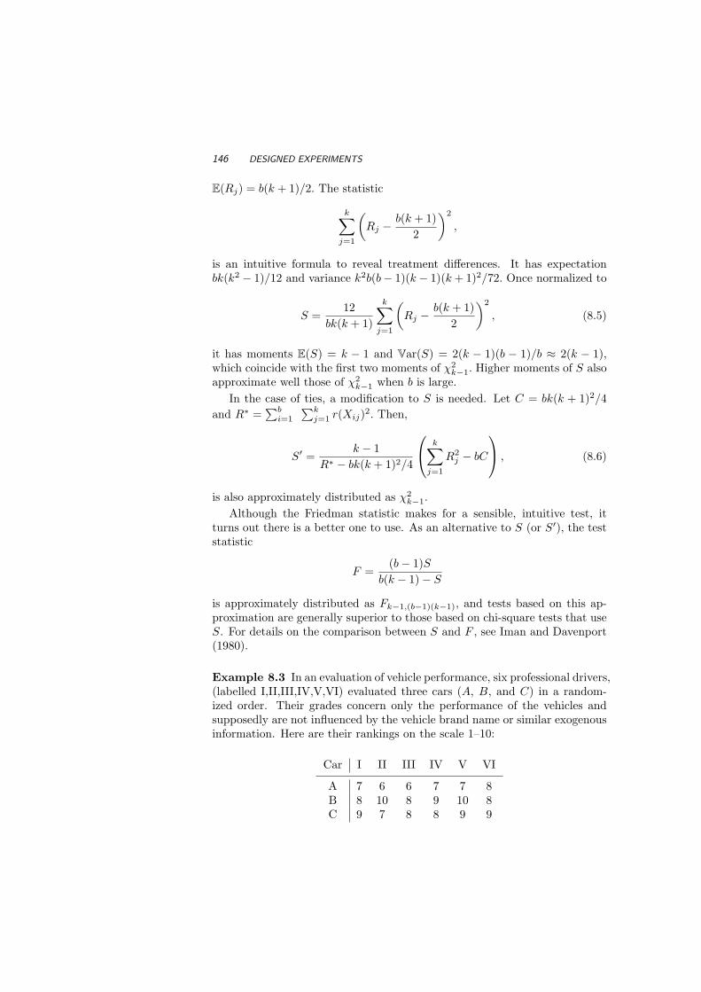
146 DESIGNED EXPERIMENTS
E(Rj) = b(k + 1)/2. The statistic
k∑
j=1
(Rj − b(k + 1)
2
)2
,
is an intuitive formula to reveal treatment differences. It has expectationbk(k2 − 1)/12 and variance k2b(b− 1)(k − 1)(k + 1)2/72. Once normalized to
S =12
bk(k + 1)
k∑
j=1
(Rj − b(k + 1)
2
)2
, (8.5)
it has moments E(S) = k − 1 and Var(S) = 2(k − 1)(b − 1)/b ≈ 2(k − 1),which coincide with the first two moments of χ2
k−1. Higher moments of S alsoapproximate well those of χ2
k−1 when b is large.In the case of ties, a modification to S is needed. Let C = bk(k + 1)2/4
and R∗ =∑b
i=1
∑kj=1 r(Xij)2. Then,
S′ =k − 1
R∗ − bk(k + 1)2/4
k∑
j=1
R2j − bC
, (8.6)
is also approximately distributed as χ2k−1.
Although the Friedman statistic makes for a sensible, intuitive test, itturns out there is a better one to use. As an alternative to S (or S′), the teststatistic
F =(b− 1)S
b(k − 1)− S
is approximately distributed as Fk−1,(b−1)(k−1), and tests based on this ap-proximation are generally superior to those based on chi-square tests that useS. For details on the comparison between S and F , see Iman and Davenport(1980).
Example 8.3 In an evaluation of vehicle performance, six professional drivers,(labelled I,II,III,IV,V,VI) evaluated three cars (A, B, and C) in a random-ized order. Their grades concern only the performance of the vehicles andsupposedly are not influenced by the vehicle brand name or similar exogenousinformation. Here are their rankings on the scale 1–10:
Car I II III IV V VI
A 7 6 6 7 7 8B 8 10 8 9 10 8C 9 7 8 8 9 9
FRIEDMAN TEST 147
To use the MATLAB procedure
friedman(data),
the first input vector represents blocks (drivers) and the second representstreatments (cars).
> data = [7 8 9; 6 10 7; 6 8 8; ...
7 9 8; 7 10 9; 8 8 9];
> [S,F,pS,pF] = friedman(data)
S =
8.2727
F =
11.0976
pS =
0.0160
pF =
0.0029 % this p-value is more reliable
Friedman Pairwise Comparisons. If the p-value is small enough to war-rant multiple comparisons of treatments, we consider two treatments i and jto be different at level α if
|Ri −Rj | > t(b−1)(k−1),1−α/2
√2 · bR∗ −∑k
j=1 R2j
(b− 1)(k − 1). (8.7)
Example 8.4 From Example 8.3, the three cars (A,B,C) are considered sig-nificantly different at test level α = 0.01 (if we use the F -statistic). We canuse the MATLAB procedure
friedman pairwise comparison(x,i,j,a)
to make a pairwise comparison between treatment i and treatment j at levela. The output = 1 if the treatments i and j are different, otherwise it is 0.The Friedman pairwise comparison reveals that car A is rated significantlylower than both car B and car C, but car B and car C are not considered tobe different.
An alternative test for k matched populations is the test by Quade (1966),which is an extension of the Wilcoxon signed-rank test. In general, the Quadetest performs no better than Friedman’s test, but slightly better in the casek = 3. For that reason, we reference it but will not go over it in any detail.
148 DESIGNED EXPERIMENTS
8.3 VARIANCE TEST FOR SEVERAL POPULATIONS
In the last chapter, the test for variances from two populations was achievedwith the nonparametric Conover Test. In this section, the test is extended tothree or more populations using a set-up similar to that of the Kruskal-Wallistest. For the hypotheses H0 : k variances are equal versus H1 : some of thevariances are different, let ni = the number of observations sampled from eachpopulation and Xij is the jth observation from population i. We denote thefollowing:
• n = n1 + · · ·+ nk
• xi = sample average for ith population
• R(xij) = rank of (xij − xi)2 among n items
• Ti =∑ni
j=1 R(xij)2
• T = n−1∑k
j=1 Tj
• VT = (n− 1)−1(∑
i
∑j R(xij)4 − nT 2
)
Then the test statistic is
T =
∑kj=1(T
2j /nj)− nT 2
VT. (8.8)
Under H0, T has an approximate χ2 distribution with k − 1 degrees offreedom, so we can test for equal variances at level α by rejecting H0 ifT > χ2
k−1(1 − α). Conover (1999) notes that the asymptotic relative effi-ciency, relative to the regular test for different variances is 0.76 (when thedata are actually distributed normally). If the data are distributed as double-exponential, the A.R.E. is over 1.08.
Example 8.5 For the crop data in the Example 8.1, we can apply the vari-ance test and obtain n = 34, T1 = 3845, T2 = 4631, T3 = 4032, T4 = 1174.5,
and T = 402.51. The variance term VT =(∑
i
∑j R(xij)4 − 34(402.51)2
)/33 =
129, 090 leads to the test statistic
T =
∑kj=1(T
2j /nj)− 34(402.51)2
VT= 4.5086.
Using the approximation that T ∼ χ23 under the null hypothesis of equal
variances, the p-value associated with this test is P (T > 4.5086) = 0.2115.There is no strong evidence to conclude the underlying variances for cropyields are significantly different.

EXERCISES 149
Multiple Comparisons. If H0 is rejected, we can determine which popula-tions have unequal variances using the following paired comparisons:
∣∣∣∣Ti
ni− Tj
nj
∣∣∣∣ >
√(1ni
+1nj
)VT
(n− 1− T
n− k
)tn−k(1− α/2),
where tn−k(α) is the α quantile of the t distribution with n − k degrees offreedom. If there are no ties, T and VT are simple constants: T = (n+1)(2n+1)/6 and VT = n(n + 1)(2n + 1)(8n + 11)/180.
8.4 EXERCISES
8.1. Show, that when ties are not present, the Kruskal-Wallis statistic H ′ in(8.2) coincides with H in (8.3).
8.2. Generate three samples of size 10 from an exponential distribution withλ = 0.10. Perform both the F -test and the Kruskal-Wallis test to seeif there are treatment differences in the three groups. Repeat this 1000times, recording the p-value for both tests. Compare the simulation re-sults by comparing the two histograms made from these p-values. Whatdo the results mean?
8.3. The data set Hypnosis contains data from a study investigating whetherhypnosis has the same effect on skin potential (measured in millivolts)for four emotions (Lehmann, p. 264). Eight subjects are asked to displayfear, joy, sadness, and calmness under hypnosis. The data are recordedas one observation per subject for each emotion.
1 fear 23.1 1 joy 22.7 1 sadness 22.5 1 calmness 22.6
2 fear 57.6 2 joy 53.2 2 sadness 53.7 2 calmness 53.1
3 fear 10.5 3 joy 9.7 3 sadness 10.8 3 calmness 8.3
4 fear 23.6 4 joy 19.6 4 sadness 21.1 4 calmness 21.6
5 fear 11.9 5 joy 13.8 5 sadness 13.7 5 calmness 13.3
6 fear 54.6 6 joy 47.1 6 sadness 39.2 6 calmness 37.0
7 fear 21.0 7 joy 13.6 7 sadness 13.7 7 calmness 14.8
8 fear 20.3 8 joy 23.6 8 sadness 16.3 8 calmness 14.8
8.4. The points-per-game statistics from the 1993 NBA season were analyzedfor basketball players who went to college in four particular ACC schools:Duke, North Carolina, North Carolina State, and Georgia Tech. Wewant to find out if scoring is different for the players from differentschools. Can this be analyzed with a parametric procedure? Why orwhy not? The classical F -test that assumes normality of the populationsyields F = 0.41 and H0 is not rejected. What about the nonparametricprocedure?

150 DESIGNED EXPERIMENTS
Duke UNC NCSU GT
7.5 5.5 16.9 7.98.7 6.2 4.5 7.87.1 13.0 10.5 14.518.2 9.7 4.4 6.1
12.9 4.6 4.05.9 18.7 14.01.9 8.7
15.8
8.5. Some varieties of nematodes (roundworms that live in the soil and arefrequently so small they are invisible to the naked eye) feed on the rootsof lawn grasses and crops such as strawberries and tomatoes. This pest,which is particularly troublesome in warm climates, can be treated bythe application of nematocides. However, because of size of the worms,it is difficult to measure the effectiveness of these pesticides directly. Tocompare four nematocides, the yields of equal-size plots of one variety oftomatoes were collected. The data (yields in pounds per plot) are shownin the table. Use a nonparametric test to find out which nematocidesare different.
Nematocide A Nematocide B Nematocide C Nematocide D
18.6 18.7 19.4 19.018.4 19.0 18.9 18.818.4 18.9 19.5 18.618.5 18.5 19.1 18.717.9 18.5
8.6. An experiment was run to determine whether four specific firing tem-peratures affect the density of a certain type of brick. The experimentled to the following data. Does the firing temperature affect the densityof the bricks?
Temperature Density
100 21.8 21.9 21.7 21.7 21.6 21.7125 21.7 21.4 21.5 21.4150 21.9 21.8 21.8 21.8 21.6 21.5175 21.9 21.7 21.8 21.4
8.7. A chemist wishes to test the effect of four chemical agents on the strengthof a particular type of cloth. Because there might be variability from onebolt to another, the chemist decides to use a randomized block design,

EXERCISES 151
with the bolts of cloth considered as blocks. She selects five bolts andapplies all four chemicals in random order to each bolt. The resultingtensile strengths follow. How do the effects of the chemical agents differ?
Bolt Bolt Bolt Bolt BoltChemical No. 1 No. 2 No. 3 No. 4 No. 5
1 73 68 74 71 672 73 67 75 72 703 75 68 78 73 684 73 71 75 75 69
8.8. The venerable auction house of Snootly & Snobs will soon be puttingthree fine 17th-and 18th-century violins, A, B, and C, up for bidding. Acertain musical arts foundation, wishing to determine which of these in-struments to add to its collection, arranges to have them played by eachof 10 concert violinists. The players are blindfolded, so that they can-not tell which violin is which; and each plays the violins in a randomlydetermined sequence (BCA, ACB, etc.)
The violinists are not informed that the instruments are classic mas-terworks; all they know is that they are playing three different violins.After each violin is played, the player rates the instrument on a 10-pointscale of overall excellence (1 = lowest, 10 = highest). The players aretold that they can also give fractional ratings, such as 6.2 or 4.5, ifthey wish. The results are shown in the table below. For the sake ofconsistency, the n = 10 players are listed as “subjects.”
SubjectViolin 1 2 3 4 5 6 7 8 9 10
A 9 9.5 5 7.5 9.5 7.5 8 7 8.5 6B 7 6.5 7 7.5 5 8 6 6.5 7 7C 6 8 4 6 7 6.5 6 4 6.5 3
8.9. From Exercise 8.5, test to see if the underlying variances for the fourplot yields are the same. Use a test level of α = 0.05.

152 DESIGNED EXPERIMENTS
REFERENCES
Friedman, M. (1937), “The Use of Ranks to Avoid the Assumption of Nor-mality Implicit in the Analysis of Variance,” Journal of the AmericanStatistical Association, 32, 675-701.
Iman, R. L., and Davenport, J. M. (1980), “Approximations of the Criti-cal Region of the Friedman Statistic,” Communications in Statistics A:Theory and Methods, 9, 571-595.
Kruskal, W. H. (1952), “A Nonparametric Test for the Several Sample Prob-lem,” Annals of Mathematical Statistics, 23, 525-540.
Kruskal W. H., and Wallis W. A. (1952), “Use of Ranks in One-CriterionVariance Analysis,” Journal of the American Statistical Association, 47,583-621.
Lehmann, E. L. (1975), Testing Statistical Hypotheses, New York: Wiley.Quade, D. (1966), “On the Analysis of Variance for the k-sample Population,”
Annals of Mathematical Statistics, 37, 1747-1785.

9Categorical Data
Statistically speaking, U.S. soldiers have less of a chance of dying fromall causes in Iraq than citizens have of being murdered in California,which is roughly the same geographical size. California has more than2300 homicides each year, which means about 6.6 murders each day.Meanwhile, U.S. troops have been in Iraq for 160 days, which meansthey’re incurring about 1.7 deaths, including illness and accidents eachday.1
Brit Hume, Fox News, August 2003.
A categorical variable is a variable which is nominal or ordinal in scale. Ordinalvariables have more information than nominal ones because their levels canbe ordered. For example, an automobile could be categorized in an ordinalscale (compact, mid-size, large) or a nominal scale (Honda, Buick, Audi).Opposed to interval data, which are quantitative, nominal data are qualitative,so comparisons between the variables cannot be described mathematically.Ordinal variables are more useful than nominal ones because they can possiblybe ranked, yet they are not quite quantitative. Categorical data analysis isseemingly ubiquitous in statistical practice, and we encourage readers whoare interested in a more comprehensive coverage to consult monographs by
1By not taking the total population of each group into account, Hume failed to note therelative risk of death (Section 9.2) to a soldier in Iraq was 65 times higher than the murderrate in California.
153

154 CATEGORICAL DATA
Agresti (1996) and Simonoff (2003).At the turn of the 19th century, while probabilists in Russia, France and
other parts of the world were hastening the development of statistical theorythrough probability, British academics made great methodological develop-ments in statistics through applications in the biological sciences. This wasdue in part from the gush of research following Charles Darwin’s publica-tion of The Origin of Species in 1859. Darwin’s theories helped to catalyzeresearch in the variations of traits within species, and this strongly affectedthe growth of applied statistics and biometrics. Soon after, Gregor Mendel’sprevious findings in genetics (from over a generation before Darwin) were“rediscovered” in light of these new theories of evolution.
(a) (b)
Fig. 9.1 Charles Darwin (1843–1927), Gregor Mendel (1780–1880)
When it comes to the development of statistical methods, two individu-als are dominant from this era: Karl Pearson and R. A. Fisher. Both werecantankerous researchers influenced by William S. Gosset, the man who de-rived the (Student’s) t distribution. Karl Pearson, in particular, contributedseminal results to the study of categorical data, including the chi-square testof statistical significance (Pearson, 1900). Fisher used Mendel’s theories as aframework for the research of biological inheritance2. Both researchers weremotivated by problems in heredity, and both played an interesting role in itspromotion.
Fisher, an upper-class British conservative and intellectual, theorized thedecline of western civilization due to the diminished fertility of the upperclasses. Pearson, his rival, was a staunch socialist, yet ironically advocateda “war on inferior races”, which he often associated with the working class.Pearson said, “no degenerate and feeble stock will ever be converted into
2Actually, Fisher showed statistically that Mendel’s data were probably fudged a little inorder to support the theory for his new genetic model. See Section 9.2.

CHI-SQUARE AND GOODNESS-OF-FIT 155
(a) (b) (c)
Fig. 9.2 Karl Pearson (1857–1936), William Sealy Gosset (a.k.a. Student) (1876–1937), and Ronald Fisher (1890–1962)
healthy and sound stock by the accumulated effects of education, good lawsand sanitary surroundings.” Although their research was undoubtedly bril-liant, racial bigotry strongly prevailed in western society during this colonialperiod, and scientists were hardly exceptional in this regard.
9.1 CHI-SQUARE AND GOODNESS-OF-FIT
Pearson’s chi-square statistic found immediate applications in biometry, ge-netics and other life sciences. It is introduced in the most rudimentary sciencecourses. For instance, if you are at a party and you meet a college graduateof the social sciences, it’s likely one of the few things they remember aboutthe required statistics class they suffered through in college is the term “chi-square”.
To motivate the chi-square statistic, let X1, X2, . . . , Xn be a sample fromany distribution. As in Chapter 6, we would like to test the goodness-of-fithypothesis H0 : FX(x) = F0(x). Let the domain of the distribution D = (a, b)be split into r non-overlapping intervals, I1 = (a, x1], I2 = (x1, x2] . . . Ir =(xr−1, b). Such intervals have (theoretical) probabilities p1 = F0(x1)− F0(a),p2 = F0(x2)− F0(x1), . . . , pr = F0(b)− F0(xr−1), under H0.
Let n1, n2, . . . , nr be observed frequencies of intervals I1, I2, . . . , Ir. In thisnotation, n1 is the number of elements of the sample X1, . . . , Xn that fallsinto the interval I1. Of course, n1 + · · · + nr = n because the intervals area partition of the domain of the sample. The discrepancy between observedfrequencies ni and theoretical frequencies npi is the rationale for forming thestatistic

156 CATEGORICAL DATA
X2 =r∑
i=1
(ni − npi)2
npi, (9.1)
that has a chi-square (χ2) distribution with r − 1 degrees of freedom. Largevalues of X2 are critical for H0. Alternative representations include
X2 =r∑
i=1
n2i
npi− n and X2 = n
[r∑
i=1
(pi
pi
)pi − 1
],
where pi = ni/n.
In some experiments, the distribution under H0 cannot be fully specified;for example, one might conjecture the data are generated from a normal distri-bution without knowing the exact values of µ or σ2. In this case, the unknownparameters are estimated using the sample.
Suppose that k parameters are estimated in order to fully specify F0. Then,the resulting statistic in (9.1) has a χ2 distribution with r − k − 1 degrees offreedom. A degree of freedom is lost with the estimation of a parameter. Infairness, if we estimated a parameter and then inserted it into the hypothesiswithout further acknowledgment, the hypothesis will undoubtedly fit the dataat least as well as any alternative hypothesis we could construct with a knownparameter. So the lost degree of freedom represents a form of handicapping.
There is no orthodoxy in selecting the categories or even the number ofcategories to use. If possible, make the categories approximately equal inprobability. Practitioners may want to arrange interval selection so that allnpi > 1 and that at least 80% of the npi’s exceed 5. The rule-of-thumb is:n ≥ 10, r ≥ 3, n2/r ≥ 10, npi ≥ 0.25.
As mentioned in Chapter 6, the chi-square test is not altogether efficientfor testing known continuous distributions, especially compared to individ-ualized tests such as Shapiro-Wilk or Anderson-Darling. Its advantage ismanifest with discrete data and special distributions that cannot be fit in aKolmogorov-type statistical test.
Example 9.1 Mendel’s Data. In 1865, Mendel discovered a basic geneticcode by breeding green and yellow peas in an experiment. Because the yellowpea gene is dominant, the first generation hybrids all appeared yellow, butthe second generation hybrids were about 75% yellow and 25% green. Thegreen color reappears in the second generation because there is a 25% chancethat two peas, both having a yellow and green gene, will contribute the greengene to the next hybrid seed. In another pea experiment3 that consideredboth color and texture traits, the outcomes from repeated experiments cameout as in Table 9.11
3See Section 16.1 for more detail on probability models in basic genetics.

CHI-SQUARE AND GOODNESS-OF-FIT 157
Table 9.11 Mendel’s Data
Type of Observed ExpectedPea Number Number
Smooth Yellow 315 313Wrinkled Yellow 101 104Smooth Green 108 104Wrinkled Green 32 35
The statistical analysis shows a strong agreement with the hypothesized out-come with a p-value of 0.9166. While this, by itself, is not sufficient proofto consider foul play, Fisher noted this kind of result in a sequence of severalexperiments. His “meta-analysis” (see Chapter 6) revealed a p-value around0.00013.
>> o=[315 101 108 32];
>> th=[313 104 104 35];
>> sum( (o-th).^2 ./ th )
ans =
0.5103
>> 1-chi2cdf( 0.5103, 4 - 1)
ans =
0.9166
Example 9.2 Horse-Kick Fatalities. During the latter part of the nine-teenth century, Prussian officials collected information on the hazards thathorses posed to cavalry soldiers. A total of 10 cavalry corps were monitoredover a period of 20 years. Recorded for each year and each corps was X, thenumber of fatalities due to kicks. Table 9.12 shows the distribution of X forthese 200 “corps-years”.
Altogether there were 122 fatalities (109(0) + 65 (1) + 22(2) + 3(3) +1(4)), meaning that the observed fatality rate was 122/200 = 0.61 fatalitiesper corps-year. A Poisson model for X with a mean of µ = .61 was proposed byvon Bortkiewicz (1898). Table 9.12 shows the expected frequency correspond-ing to x = 0, 1, . . . , etc., assuming the Poisson model for X was correct. Theagreement between the observed and the expected frequencies is remarkable.The MATLAB procedure below shows that the resulting X2 statistic = 0.6104.If the Poisson distribution is correct, the statistic is distributed χ2 with 3 de-grees of freedom, so the p-value is computed P (W > 0.6104) = 0.8940.
>> o=[109 65 22 3 1];

158 CATEGORICAL DATA
Table 9.12 Horse-kick fatalities data
Observed Number Expected Numberx of Corps-Years of Corps-Years
0 109 108.71 65 66.32 22 20.23 3 4.14 1 0.7
200 200
>> th=[108.7 66.3 20.2 4.1 0.7];
>> sum( (o-th).^2 ./ th )
ans = 0.6104
>> 1-chi2cdf( 0.6104, 5 - 1 - 1)
ans = 0.8940
Example 9.3 Benford’s Law. Benford’s law (Benford, 1938; Hill, 1998)concerns relative frequencies of leading digits of various data sets, numericaltables, accounting data, etc. Benford’s law, also called the first digit law,states that in numbers from many sources, the leading digit 1 occurs muchmore often than the others (namely about 30% of the time). Furthermore, thehigher the digit, the less likely it is to occur as the leading digit of a number.This applies to figures related to the natural world or of social significance, beit numbers taken from electricity bills, newspaper articles, street addresses,stock prices, population numbers, death rates, areas or lengths of rivers orphysical and mathematical constants.
To be precise, Benford’s law states that the leading digit n, (n = 1, . . . , 9)occurs with probability P (n) = log10(n+1)− log10(n), approximated to threedigits in the table below.
Digit n 1 2 3 4 5 6 7 8 9
P (n) 0.301 0.176 0.125 0.097 0.079 0.067 0.058 0.051 0.046
The table below lists the distribution of the leading digit for all 307 numbersappearing in a particular issue of Reader’s Digest. With p-value of 0.8719, thesupport for H0 (The first digits in Reader’s Digest are distributed accordingto Benford’s Law) is strong.
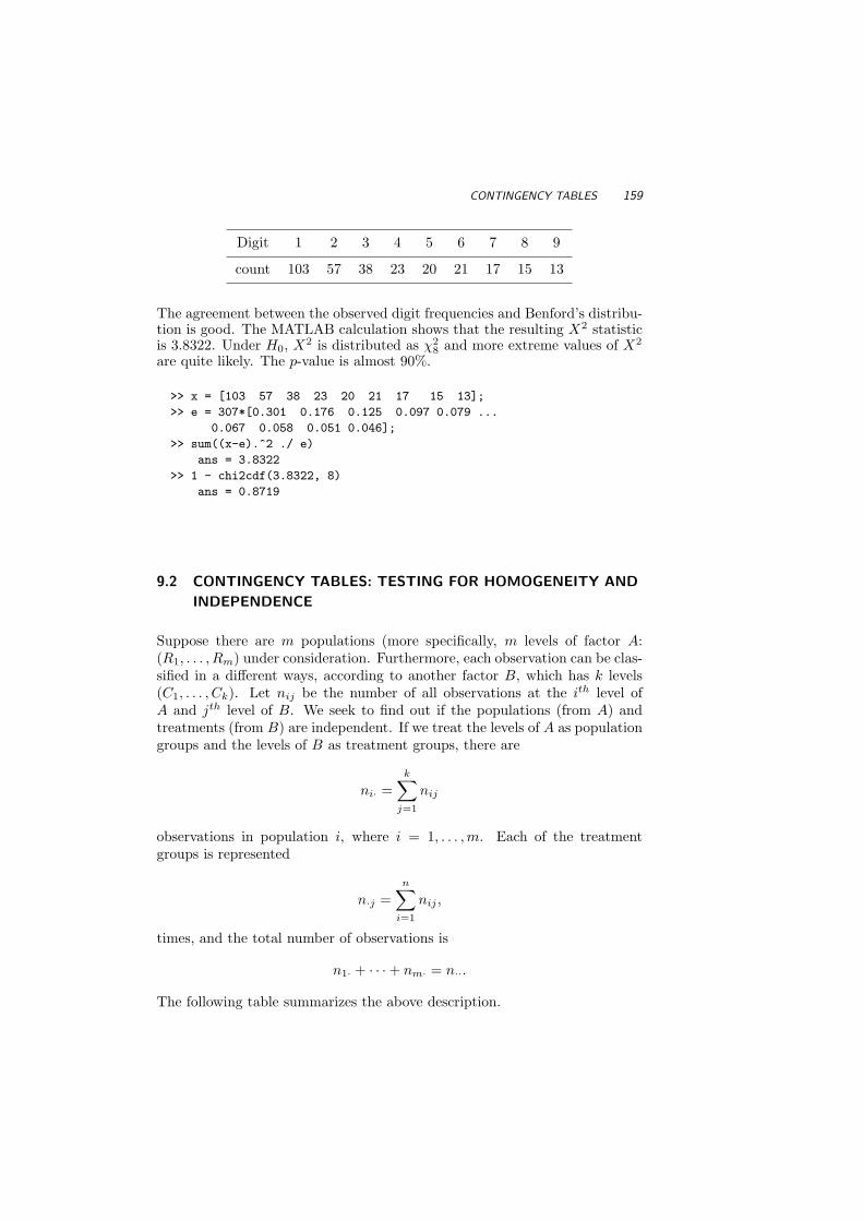
CONTINGENCY TABLES 159
Digit 1 2 3 4 5 6 7 8 9
count 103 57 38 23 20 21 17 15 13
The agreement between the observed digit frequencies and Benford’s distribu-tion is good. The MATLAB calculation shows that the resulting X2 statisticis 3.8322. Under H0, X2 is distributed as χ2
8 and more extreme values of X2
are quite likely. The p-value is almost 90%.
>> x = [103 57 38 23 20 21 17 15 13];
>> e = 307*[0.301 0.176 0.125 0.097 0.079 ...
0.067 0.058 0.051 0.046];
>> sum((x-e).^2 ./ e)
ans = 3.8322
>> 1 - chi2cdf(3.8322, 8)
ans = 0.8719
9.2 CONTINGENCY TABLES: TESTING FOR HOMOGENEITY AND
INDEPENDENCE
Suppose there are m populations (more specifically, m levels of factor A:(R1, . . . , Rm) under consideration. Furthermore, each observation can be clas-sified in a different ways, according to another factor B, which has k levels(C1, . . . , Ck). Let nij be the number of all observations at the ith level ofA and jth level of B. We seek to find out if the populations (from A) andtreatments (from B) are independent. If we treat the levels of A as populationgroups and the levels of B as treatment groups, there are
ni· =k∑
j=1
nij
observations in population i, where i = 1, . . . , m. Each of the treatmentgroups is represented
n·j =n∑
i=1
nij ,
times, and the total number of observations is
n1· + · · ·+ nm· = n··.
The following table summarizes the above description.

160 CATEGORICAL DATA
C1 C2 · · · Ck Total
R1 n11 n12 n1k n1·
R2 n21 n22 n2k n2·
Rm nm1 nm2 nmk nm·
Total n·1 n·2 n·k n··
We are interested in testing independence of factors A and B, representedby their respective levels R1, . . . , Rm and C1, . . . , Ck, on the basis of observedfrequencies nij . Recall the definition of independence of component randomvariables X and Y in the random vector (X,Y ),
P (X = xi, Y = yj) = P (X = xi) · P (Y = yj).
Assume that the random variable ξ is to be classified. Under the hypothesisof independence, the cell probabilities P (ξ ∈ Ri ∩ Cj) should be equal to theproduct of probabilities P (ξ ∈ Ri) ·P (ξ ∈ Cj). Thus, to test the independenceof factors A and B, we should evaluate how different the sample counterpartsof cell probabilities
nij
n··are from the product of marginal probability estimators:
ni·n··
· n·jn··
,
or equivalently, how different the observed frequencies, nij , are from the ex-pected (under the hypothesis of independence) frequencies
nij = n··ni·n··
n·jn··
=ni· · n·j
n··.
The measure of discrepancy, defined as
X2 =m∑
i=1
k∑
j=1
(nij − nij)2
nij, (9.2)
and under the assumption of independence, (9.2) has a χ2 distribution with(m − 1)(k − 1) degrees of freedom. Here is the rationale: the observedfrequencies nij are distributed as multinomial Mn(n··; θ11, . . . , θmk), whereθij = P (ξ ∈ Ri ∩ Cj).

CONTINGENCY TABLES 161
C1 C2 · · · Ck Total
R1 θ11 θ12 θ1k θ1·
R2 θ21 θ22 θ2k θ2·
Rm θm1 θm2 θmk θm·
Total θ·1 θ·2 θ·k 1
The corresponding likelihood is L =∏m
i=1
∏kj=1(θij)nij ,
∑i,j θij = 1.
The null hypothesis of independence states that for any pair i, j, the cellprobability is the product of marginal probabilities, θij = θi· · θ·j . Under H0
the likelihood becomes
L =m∏
i=1
n∏
j=1
(θi· · θ·j)nij ,∑
i
θi· =∑
j
θ·j = 1.
If the estimators of θi· and θ·j are θi· = ni·/n·· and θ·j = n·j/n··, respec-tively, then, under H0, the observed frequency nij should be compared to itstheoretical counterpart,
nij = θijn·· =ni·n·jn··
.
As the nij are binomially distributed, they can be approximated by thenormal distribution, and the χ2 forms when they are squared. The statisticis based on (m − 1) + (k − 1) estimated parameters, θi·, i = 1, . . . , m − 1,and θ·j , j = 1, . . . , k − 1. The remaining parameters are determined: θm· =1−∑m−1
i=1 θi·, θ·n = 1−∑k−1n=1 θ·j . Thus, the chi-square statistic
χ2 =m∑
i=1
k∑
j=1
(nij − nij)2
nij
has mk − 1− (m− 1)− (k − 1) = (m− 1)(k − 1) degrees of freedom.Pearson first developed this test but mistakenly used mk − 1 degrees of
freedom. It was Fisher (1922), who later deduced the correct degrees of free-dom, (m− 1)(k − 1). This probably did not help to mitigate the antagonismin their professional relationship!
Example 9.4 Icelandic Dolphins. From Rasmussen and Miller (2004),groups of dolphins were observed off the coast in Iceland, and their frequencyof observation was recorded along with the time of day and the perceivedactivity of the dolphins at that time. Table 9.13 provides the data. To see if

162 CATEGORICAL DATA
the activity is independent of the time of day, the MATLAB procedure
tablerxc(X)
takes the input table X and computes the χ2 statistic, its associated p-value,and a table of expected values under the assumption of independence. In thisexample, the activity and time of day appear to be dependent.
Table 9.13 Observed Groups of Dolphins, Including Time of Day and Activity
Time-of-Day Traveling Feeding Socializing
Morning 6 28 38Noon 6 4 5
Afternoon 14 0 9Evening 13 56 10
>>[chi2,pvalue,exp]=tablerxc([6 28 38; 6 4 5; 14 0 9; 13 56 10])
chi2 =
68.4646
pvalue =
8.4388e-013
exp =
14.8571 33.5238 23.6190
3.0952 6.9841 4.9206
4.7460 10.7090 7.5450
16.3016 36.7831 25.9153
Relative Risk. In simple 2 × 2 tables, the comparison of two proportionsmight be more important if those proportions veer toward zero or one. Forexample, a procedure that decreases production errors from 5% to 2% couldbe much more valuable than one that decreases errors in another process from45% to 42%. For example, if we revisit the example introduced at the start ofthe chapter, the rate of murder in California is compared to the death rate ofU.S. military personnel in Iraq in 2003. The relative risk, in this case, is rathereasy to understand (even to the writers at Fox News), if overly simplified.
Killed Not Killed Total
California 6.6 37,999,993.4 38,000,000Iraq 1.7 149,998.3 150,000
Total 8.3 38,149,981.7

FISHER EXACT TEST 163
Here we define the relative risk as the risk of death in Iraq (for U.S. sol-diers) divided by the risk of murder for citizens of California. For example,McWilliams and Piotrowski (2005) determined the rate of 6.6 Californianhomicide victims (out of 38,000,000 at risk) per day. On the other hand,there were 1.7 average daily military related deaths in Iraq (with 150,000solders at risk).
θ11
θ11 + θ12
(θ21
θ21 + θ22
)−1
=1.7
150, 000
(6.6
38, 000, 000
)−1
= 65.25.
Fixed Marginal Totals. The categorical analysis above was developedbased on assuming that each observation is to be classified according to thestochastic nature of the two factors. It is actually common, however, to haveeither row or column totals fixed. If row totals are fixed, for example, we areobserving nj. observations distributed into k bins, and essentially comparingmultinomial observations. In this case we are testing differences in the multi-nomial parameter sets. However, if we look at the experiment this way (wherenj is fixed) the test statistic and rejection region remain the same. This isalso true if both row and column totals are fixed. This is less common; forexample, if m = k = 2, this is essentially Fisher’s exact test.
9.3 FISHER EXACT TEST
Along with Pearson, R. A. Fisher contributed important new methods foranalyzing categorical data. Pearson and Fisher both recognized that the sta-tistical methods of their time were not adequate for small categorized samples,but their disagreements are more well known. In 1922, Pearson, used his po-sition as editor of Biometrika to attack Fisher’s use of the chi-squared test.Fisher attacked Pearson with equal fierceness. While at University College,Fisher continued to criticize Pearson’s ideas even after his passing. WithPearson’s son Egon also holding a chair there, the departmental politics wereawkward, to say the least.
Along with his original concept of maximum likelihood estimation, Fisherpioneered research in small sample analysis, including a simple categoricaldata test that bears his name (Fisher Exact Test). Fisher (1966) described atest based on the claims of a British woman who said she could taste a cup oftea, with milk added, and identify whether the milk or tea was added to thecup first. She was tested with eight cups, of which she knew four had the teaadded first, and four had the milk added first. The results are listed below.
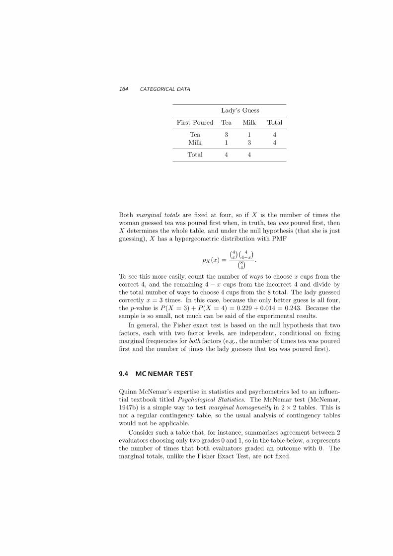
164 CATEGORICAL DATA
Lady’s Guess
First Poured Tea Milk Total
Tea 3 1 4Milk 1 3 4
Total 4 4
Both marginal totals are fixed at four, so if X is the number of times thewoman guessed tea was poured first when, in truth, tea was poured first, thenX determines the whole table, and under the null hypothesis (that she is justguessing), X has a hypergeometric distribution with PMF
pX(x) =
(4x
)(4
4−x
)(84
) .
To see this more easily, count the number of ways to choose x cups from thecorrect 4, and the remaining 4 − x cups from the incorrect 4 and divide bythe total number of ways to choose 4 cups from the 8 total. The lady guessedcorrectly x = 3 times. In this case, because the only better guess is all four,the p-value is P (X = 3) + P (X = 4) = 0.229 + 0.014 = 0.243. Because thesample is so small, not much can be said of the experimental results.
In general, the Fisher exact test is based on the null hypothesis that twofactors, each with two factor levels, are independent, conditional on fixingmarginal frequencies for both factors (e.g., the number of times tea was pouredfirst and the number of times the lady guesses that tea was poured first).
9.4 MCNEMAR TEST
Quinn McNemar’s expertise in statistics and psychometrics led to an influen-tial textbook titled Psychological Statistics. The McNemar test (McNemar,1947b) is a simple way to test marginal homogeneity in 2 × 2 tables. This isnot a regular contingency table, so the usual analysis of contingency tableswould not be applicable.
Consider such a table that, for instance, summarizes agreement between 2evaluators choosing only two grades 0 and 1, so in the table below, a representsthe number of times that both evaluators graded an outcome with 0. Themarginal totals, unlike the Fisher Exact Test, are not fixed.

MCNEMAR TEST 165
0 1 total
0 a b a + b1 c d c + d
total a + c b + d a + b + c + d
Marginal homogeneity (i.e., the graders give the same proportion of zerosand ones, on average) implies that row totals should be close to the corre-sponding column totals, or
a + b ≈ a + c (9.3)c + d ≈ b + d.
More formally, suppose that a matched pair of Bernoulli random variables(X,Y ) is to be classified into a table,
0 1 marginal
0 θ00 θ01 θ0·1 θ10 θ11 θ1·
marginal θ·0 θ·1 1
in which θij = P (X = i, Y = j), θi· = P (X = i) and θ·j = P (Y = j), fori, j ∈ 0, 1. The null hypothesis H0 can be expressed as a hypothesis ofsymmetry
H0 : θ01 = P (X = 0, Y = 1) = P (X = 1, Y = 0) = θ10, (9.4)
but after adding θ00 = P (X = 0, Y = 0) or θ11 = P (X = 1, Y = 1) to theboth sides in (9.4), we get H0 in the form of marginal homogeneity,
H0 : θ0· = P (X = 0) = P (Y = 0) = θ·0, or equivalentlyH0 : θ1· = P (X = 1) = P (Y = 1) = θ·1 .
As a and d on both sides of (9.3) cancel out, implying b ≈ c. A sensible teststatistic for testing H0 might depend on how much b and c differ. The valuesof a and d are called ties and do not contribute to the testing of H0.
When, b + c > 20, the McNemar statistic is calculated as
X2 =(b− c)2
b + c,
which has a χ2 distribution with 1 degree of freedom. Some authors rec-ommend a version of the McNemar test with a correction for discontinuity,
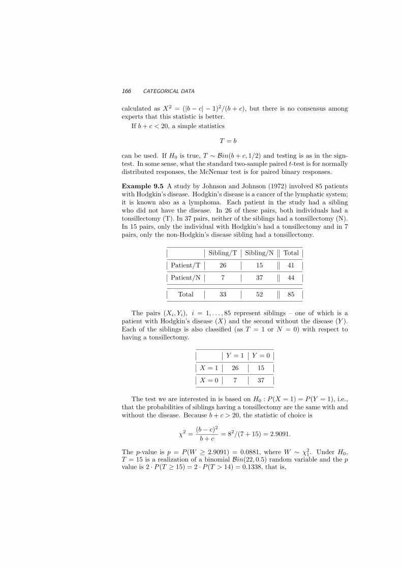
166 CATEGORICAL DATA
calculated as X2 = (|b − c| − 1)2/(b + c), but there is no consensus amongexperts that this statistic is better.
If b + c < 20, a simple statistics
T = b
can be used. If H0 is true, T ∼ Bin(b + c, 1/2) and testing is as in the sign-test. In some sense, what the standard two-sample paired t-test is for normallydistributed responses, the McNemar test is for paired binary responses.
Example 9.5 A study by Johnson and Johnson (1972) involved 85 patientswith Hodgkin’s disease. Hodgkin’s disease is a cancer of the lymphatic system;it is known also as a lymphoma. Each patient in the study had a siblingwho did not have the disease. In 26 of these pairs, both individuals had atonsillectomy (T). In 37 pairs, neither of the siblings had a tonsillectomy (N).In 15 pairs, only the individual with Hodgkin’s had a tonsillectomy and in 7pairs, only the non-Hodgkin’s disease sibling had a tonsillectomy.
Sibling/T Sibling/N Total
Patient/T 26 15 41
Patient/N 7 37 44
Total 33 52 85
The pairs (Xi, Yi), i = 1, . . . , 85 represent siblings – one of which is apatient with Hodgkin’s disease (X) and the second without the disease (Y ).Each of the siblings is also classified (as T = 1 or N = 0) with respect tohaving a tonsillectomy.
Y = 1 Y = 0
X = 1 26 15
X = 0 7 37
The test we are interested in is based on H0 : P (X = 1) = P (Y = 1), i.e.,that the probabilities of siblings having a tonsillectomy are the same with andwithout the disease. Because b + c > 20, the statistic of choice is
χ2 =(b− c)2
b + c= 82/(7 + 15) = 2.9091.
The p-value is p = P (W ≥ 2.9091) = 0.0881, where W ∼ χ21. Under H0,
T = 15 is a realization of a binomial Bin(22, 0.5) random variable and the pvalue is 2 · P (T ≥ 15) = 2 · P (T > 14) = 0.1338, that is,

COCHRAN’S TEST 167
>> 2 * (1-binocdf(14, 22, 0.5))
ans =
0.1338
With such a high p-value, there is scant evidence to reject the null hypoth-esis of homogeneity of the two groups of patients with respect to having atonsillectomy.
9.5 COCHRAN’S TEST
Cochran’s (1950) test is essentially a randomized block design (RBD), asdescribed in Chapter 8, but the responses are dichotomous. That is, eachtreatment-block combination receives a 0 or 1 response.
If there are only two treatments, the experimental outcome is equivalentto McNemar’s test with marginal totals equaling the number of blocks. Tosee this, consider the last example as a collection of dichotomous outcomes;each of the 85 patients are initially classified into two blocks depending onwhether the patient had or had not received a tonsillectomy. The response is0 if the patient’s sibling did not have a tonsillectomy and 1 if they did.
Example 9.6 Consider the software debugging data in Table 9.14. Here thesoftware reviewers (A,B,C,D,E) represent five blocks, and the 27 bugs areconsidered to be treatments. Let the column totals be denoted C1, · · · , C5and denote row totals as R1, · · · , R27. We are essentially testing H0 :treatments (software bugs) have an equal chance of being discovered, versusHa : some software bugs are more prevalent (or easily found) than others. thetest statistic is
TC =
∑mj=1
(Cj − n
m
)2
(Pki=1 Ri(m−Ri)
m(m−1)
)
where n =∑
Cj =∑
Ri, m = 5 (blocks) and k = 27 treatments (softwarebugs). Under H0, TC has an approximate chi-square distribution with m− 1degrees of freedom. In this example, TC = 17.647, corresponding to a testp-value of 0.00145.
9.6 MANTEL-HAENSZEL TEST
Suppose that k independent classifications into a 2x2 table are observed. Wecould denote the ith such table by

168 CATEGORICAL DATA
Table 9.14 Five Reviewers Found 27 Issues in Software Example as in Gilb and Gra-ham (1993)
A B C D E A B C D E
1 1 1 1 1 0 0 1 0 01 0 1 0 1 0 0 1 0 01 1 1 0 1 0 0 0 1 01 0 1 1 1 1 1 1 0 11 0 1 1 1 0 0 1 0 11 0 1 1 1 1 0 0 0 01 1 1 1 1 0 1 0 0 01 1 1 1 1 1 0 1 1 10 0 1 0 0 0 0 0 0 01 0 1 0 0 0 0 0 0 00 1 0 0 0 0 1 0 0 11 0 0 1 1 1 0 0 0 01 0 1 0 1 1 0 0 0 00 0 1 0 1
xi ri − xi ri
ci − xi ni − ri − ci + xi ni − ri
ci ni − ci ni
(a) (b) (c)
Fig. 9.3 Quinn McNemar (1900-1986), William Gemmell Cochran (1909-1980), andNathan Mantel (1919-2002)
It is assumed that the marginal totals (ri, ni or just ni) are fixed in advanceand that the sampling was carried out until such fixed marginal totals aresatisfied. If each of the k tables represent an independent study of the sameclassifications, the Mantel-Haenszel Test essentially pools the studies togetherin a “meta-analysis” that combines all experimental outcomes into a single

MANTEL-HAENSZEL TEST 169
statistic. For more about non-parametric approaches to this kind of problem,see the section on meta-analysis in Chapter 6.
For the ith table, p1i is the proportion of subjects from the first row fallingin the first column, and likewise, p2i is the proportion of subjects from the2nd row falling in the first column. The hypothesis of interest here is if thepopulation proportions p1i and p2i coincide over all k experiments.
Suppose that in experiment i there are ni observations. All items can becategorized as type 1 (ri of them) or type 2 (ni − ri of them). If ci itemsare selected from the total of ni items, the probability that exactly xi of theselected items are of the type 1 is
(ri
xi
) · (ni−ri
ci−xi
)(ni
ci
) . (9.5)
Likewise, all items can be categorized as type A (ci of them) or type B (ni−ci
of them). If ri items are selected from the total of ni items, the probabilitythat exactly xi of the selected are of the type A is
(ci
xi
) · (ni−ci
ri−xi
)(ni
ri
) . (9.6)
Of course these two probabilities are equal, i.e,(
ri
xi
) · (ni−ri
ci−xi
)(ni
ci
) =
(ci
xi
) · (ni−ci
ri−xi
)(ni
ri
) .
These are hypergeometric probabilities with mean and variance
ri · ci
ni, and
ri · ci · (ni − ri) · (ni − ci)n2
i (ni − 1),
respectively. The k experiments are independent and the statistic
T =
∑ki=1 xi −
∑ki=1
rici
ni√∑ki=1
ri·ci·(ni−ri)·(ni−ci)n2
i (ni−1)
(9.7)
is approximately normal (if ni is large, the distributions of the xi’s are closeto binomial and thus the normal approximation holds. In addition, summingover k independent experiments makes the normal approximation more accu-rate.) Large values of |T | indicate that the proportions change across the kexperiments.
Example 9.7 The three 2 × 2 tables provide classification of people from 3Chinese cities, Zhengzhou, Taiyuan, and Nanchang with respect to smokinghabits and incidence of lung cancer (Liu, 1992).

170 CATEGORICAL DATA
Zhengzhou Taiyuan Nanchang
Cancer Diagnosis: yes no total yes no total yes no total
Smoker 182 156 338 60 99 159 104 89 193Non-Smoker 72 98 170 11 43 54 21 36 57
Total 254 254 508 71 142 213 125 125 250
We can apply the Mantel-Haenszel Test to decide if the proportions ofcancer incidence for smokers and non-smokers coincide for the three cities, i.e.,H0 : p1i = p2i where p1i is the proportion of incidence of cancer among smokersin the city i, and p2i is the proportion of incidence of cancer among nonsmokersin the city i, i = 1, 2, 3. We use the two-sided alternative, H1 : p1i 6= p2i forsome i ∈ 1, 2, 3 and fix the type-I error rate at α = 0.10.
From the tables,∑
i xi = 182 + 60 + 104 = 346. Also,∑
i rici/ni =338 · 254/508 + 159 · 71/213 + 193 · 125/250 = 169 + 53 + 96.5 = 318.5. Tocompute T in (9.7),
∑
i
ri ci (ni − ri) (ni − ci)n2
i (ni − 1)=
338 · 254 · 170 · 2545082 · 507
+159 · 71 · 54 · 142
2132 · 212
+193 · 125 · 57 · 125
2502 · 249= 28.33333 + 9 + 11.04518 = 48.37851.
Therefore,
T =
∑i xi −
∑i
ri ci
ni√ ∑i
ri ci (ni−ri) (ni−ci)n2
i (ni−1)
=346− 318.5√
48.37851≈ 3.95.
Because T is approximately N (0, 1), the p-value (via MATLAB) is
>> [st, p] = mantel_haenszel([182 156; 72 98; 60 99; 11 43; 104 89; 21 36])
st = 3.9537
p = 7.6944e-005
In this case, there is clear evidence that the differences in cancer rates is notconstant across the three cities.

CLT FOR MULTINOMIAL PROBABILITIES 171
9.7 CENTRAL LIMIT THEOREM FOR MULTINOMIAL
PROBABILITIES
Let E1, E2, . . . , Er be events that have probabilities p1, p2, . . . , pr;∑
i pi = 1.Suppose that in n independent trials the event Ei appears ni times (n1 + · · ·+nr = n). Consider
ζ(n) =(√
n
p1
(n1
n− p1
), . . . ,
√n
pr
(nr
n− pr
)).
The vector ζ(n) can be represented as
ζ(n) =1√n
n∑
j=1
ξ(j),
where components ξ(j) are given by pi−1/2[1(Ei)−pi], i = 1, . . . , r. Vectors ξ(j)
are i.i.d., with E(ξ(j)i ) = pi
−1(E1(Ei)−pi) = 0, E(ξ(j)i )2 = (pi
−1)pi(1−pi) =1− pi, and E(ξ(j)
i ξ(j)` ) = (pip`)−1/2(E1(Ei)1(E`)− pip`) = −√pip`, i 6= `.
Result. When n →∞, the random vector ζ(n) is asymptotically normal withmean 0 and the covariance matrix,
Σ =
1− p1 −√p1p2 . . . −√p1pr
−√p2p1 1− p2 . . . −√p2pr
. . .−√prp1 −√prp2 . . . 1− pr
= I − zz′,
where I is the r × r identity matrix and z = (√
p1√
p2 , . . . ,√
pr)′. Thematrix Σ is singular. Indeed, Σz = z − z(z′z) = 0, due to z′z = 1.
As a consequence, λ = 0 is characteristic value of Σ corresponding to acharacteristic vector z. Because |ζ(n)|2 is a continuous function of ζ(n), itslimiting distribution is the same as |ζ|2, where |ζ|2 is distributed as χ2 withr − 1 degrees of freedom.
This is more clear if we consider the following argument. Let Ξ be anorthogonal matrix with the first row equal to (
√p1, . . . ,
√pr), and the rest
being arbitrary, but subject to orthogonality of Ξ. Let η = Ξζ. Then Eη = 0and Ση = Eηη′ = E(Ξζ)(Ξζ)′ = ΞEζζ ′Ξ′ = ΞΣΞ′ = I − (Ξz)(Ξz)′, becauseΞ′ = Ξ−1 It follows that Ξz = (1, 0, 0, . . . , 0) and (Ξz)(Ξz)′ is a matrix with

172 CATEGORICAL DATA
element at the position (1,1) as the only nonzero element. Thus,
Ση = I − (Ξz)(Ξz)′ =
0 0 0 . . . 00 1 0 . . . 00 0 1 . . . 0
. . .0 0 0 . . . 1
,
and η1 = 0, w.p.1; η2, . . . , ηr are i.i.d. N (0, 1). The orthogonal transforma-tion preserves the L2 norm,
|ζ|2 = |η|2 =r∑
i=2
η2i
d= χ2r−1.
But, |ζ(n)|2 =∑r
i=1(ni−npi)
2
npi
d→ |ζ|2.
9.8 SIMPSON’S PARADOX
Simpson’s Paradox is an example of changing the favor-ability of marginalproportions in a set of contingency tables due to aggregation of classes. In thiscase the manner of classification can be thought as a “lurking variable” causingseemingly paradoxical reversal of the inequalities in the marginal proportionswhen they are aggregated. Mathematically, there is no paradox – the set ofvectors can not be ordered in the traditional fashion.
As an example of Simpson’s Paradox, Radelet (1981) investigated the re-lationship between race and whether criminals (convicted of homicide) receivethe death penalty (versus a lesser sentence) for regional Florida court casesduring 1976–1977. Out of 326 defendants who were Caucasian or African-American, the table below shows that a higher percentage of Caucasian de-fendants (11.88%) received a death sentence than for African-American de-fendants (10.24%).
Race of Defendant Death Penalty Lesser Sentence
Caucasian 19 141African-American 17 149
Total 36 290
What the table doesn’t show you is the real story behind these statistics.The next 2 × 2 × 2 table lists the death sentence frequencies categorized bythe defendant’s race and the (murder) victim’s race. The table above is con-structed by aggregating over this new category. Once the full table is shown,we see the importance of the victim’s race in death penalty decisions. African-

EXERCISES 173
Americans were sentenced to death more often if the victim was Caucasian(17.5% versus 12.6%) or African-American (5.8% to 0.0%). Why is this so?Because of the dramatic difference in marginal frequencies (i.e., 9 Caucasiansdefendants with African-American victims versus 103 African-American de-fendants with African-American victims). When both marginal associationspoint to a single conclusion (as in the table below) but that conclusion iscontradicted when aggregating over a category, this is Simpson’s paradox.4
Race of Race of Death LesserDefendant Victim Penalty Sentence
Caucasian Caucasian 19 132African-American 0 9
African-American Caucasian 11 52African-American 6 97
9.9 EXERCISES
9.1. Duke University has always been known for its great school spirit, es-pecially when it comes to Men’s basketball. One way that school en-thusiasm is shown is by donning Duke paraphernalia including shirts,hats, shorts and sweat-shirts. A class of Duke students explored pos-sible links between school spirit (measured by the number of studentswearing paraphernalia) and some other attributes. It was hypothesizedthat males would wear Duke clothes more frequently than females. Thedata were collected on the Bryan Center walkway starting at 12:00 pmon ten different days. Each day 50 men and 50 women were tallied. Dothe data bear out this claim?
Duke Paraphernalia No Duke Paraphernalia Total
Male 131 369 500
Female 52 448 500
Total 183 817 1000
9.2. Gene Siskel and Roger Ebert hosted the most famous movie reviewshows in history. Below are their respective judgments on 43 films thatwere released in 1995. Each critic gives his judgment with a “thumbs
4Note that other covariate information about the defendant and victim, such as income orwealth, might have led to similar results

174 CATEGORICAL DATA
up” or “thumbs down.” Do they have the same likelihood of giving amovie a positive rating?
Ebert’s ReviewThumbs Up Thumbs Down
Siskel’s Thumbs Up 18 6Review Thumbs Down 9 10
9.3. Bickel, Hammel, and OConnell (1975) investigated whether there wasany evidence of gender bias in graduate admissions at the Universityof California at Berkeley. The table below comes from their cross-classification of 4,526 applications to graduate programs in 1973 bygender (male or female), admission (whether or not the applicant wasadmitted to the program) and program (A, B, C, D, E or F). What doesthe data reveal?
A: Admit Male Female
Admitted 512 89Rejected 313 19
B: Admit Male Female
Admitted 353 17Rejected 207 8
C: Admit Male Female
Admitted 120 202Rejected 205 391
D: Admit Male Female
Admitted 138 131Rejected 279 244
E: Admit Male Female
Admitted 53 94Rejected 138 299
F: Admit Male Female
Admitted 22 24Rejected 351 317
9.4. When an epidemic of severe intestinal disease occurred among workersin a plant in South Bend, Indiana, doctors said that the illness resultedfrom infection with the amoeba Entamoeba histolytica5. There are actu-ally two races of these amoebas, large and small, and the large ones were
5Source: J. E. Cohen (1973). Independence of Amoebas. In Statistics by Example: Weigh-ing Chances, edited by F. Mosteller, R. S. Pieters, W. H. Kruskal, G. R. Rising, and R. F.Link, with the assistance of R. Carlson and M. Zelinka, p. 72. Addison-Wesley: Reading,MA.

EXERCISES 175
believed to be causing the disease. Doctors suspected that the presenceof the small ones might help people resist infection by the large ones.To check on this, public health officials chose a random sample of 138apparently healthy workers and determined if they were infected witheither the large or small amoebas. The table below gives the resultingdata. Is the presence of the large race independent of the presence ofthe small one?
Large RaceSmall Race Present Absent Total
Present 12 23 35Absent 35 68 103
Total 47 91 138
9.5. A study was designed to test whether or not aggression is a functionof anonymity. The study was conducted as a field experiment on Hal-loween; 300 children were observed unobtrusively as they made theirrounds. Of these 300 children, 173 wore masks that completely coveredtheir faces, while 127 wore no masks. It was found that 101 childrenin the masked group displayed aggressive or antisocial behavior versus36 children in unmasked group. What conclusion can be drawn? Stateyour conclusion in terminology of the problem, using α = 0.01.
9.6. Deathbed scenes in which a dying mother or father holds to life untilafter the long-absent son returns home and dies immediately after areall too familiar in movies. Do such things happen in everyday life?Are some people able to postpone their death until after an anticipatedevent takes place? It is believed that famous people do so with respectto their birthdays to which they attach some importance. A study byDavid P. Phillips (in Tanur, 1972, pp. 52-65) seems to be consistentwith the notion. Phillips obtained data6 on months of birth and deathof 1251 famous Americans; the deaths were classified by the time periodbetween the birth dates and death dates as shown in the table below.What do the data suggest?
b e f o r e Birth a f t e r6 5 4 3 2 1 Month 1 2 3 4 5
90 100 87 96 101 86 119 118 121 114 113 106
6348 were people listed in Four Hundred Notable Americans and 903 are listed as foremostfamilies in three volumes of Who Was Who for the years 1951–60, 1943–50 and 1897–1942.

176 CATEGORICAL DATA
9.7. Using a calculator mimic the MATLAB results for X2 from Benford’slaw example (from p. 158). Here are some theoretical frequencies roundedto 2 decimal places:
92.41 54.06 • 29.75 24.31 • • 15.72 14.06
Use χ2 tables and compare X2 with the critical χ2 quantile at α = 0.05.
9.8. Assume that a contingency table has two rows and two columns withfrequencies of a and b in the first row and frequencies of c and d in thesecond row.
(a) Verify that the χ2 test statistic can be expressed as
χ2 =(a + b + c + d)(ad− bc)2
(a + b)(c + d)(b + d)(a + c).
(b) Let p1 = a/(a + c) and p2 = b/(b + d). Show that the test statistic
z =(p1 − p2)− 0√
pqn·1
+ pqn·2
, where p =a + b
a + b + c + d
and q = 1− p, coincides with χ2 from (a).
9.9. Generate a sample of size n = 216 from N (0, 1). Select intervals bypartitioning R at points −2.7, −2.2, −2, −1.7, −1.5, −1.2, −1, −0.8,−0.5, −0.3, 0, 0.2, 0.4, 0.9, 1, 1.4, 1.6, 1.9, 2, 2.5, and 2.8. Using aχ2-test, confirm the normality of the sample. Repeat this procedureusing sample contaminated by the Cauchy distribution in the followingway: 0.95*normal sample + 0.05*cauchy sample.
9.10. It is well known that when the arrival times of customers constitutea Poisson process with the rate λt, the inter-arrival times follow anexponential distribution with density f(t) = λe−λt, t ≥ 0, λ > 0. It isoften of interest to establish that the process is Poisson because manytheoretical results are available for such processes, ubiquitous in thedomain of Industrial Engineering.
In the following example, n = 109 inter-arrival times of an arrival processwere recorded, averaged (x = 2.5) and categorized into time intervals asfollows:
Interval [0,1) [1,2) [2,3) [3,4) [4,5) [5,6) [6,∞)
Frequency 34 20 16 15 9 7 8
EXERCISES 177
Test the hypothesis that the process described with the above inter-arrival times is Poisson, at level α = 0.05. You must first estimate λfrom the data.
9.11. In a long study of heart disease, the day of the week on which 63 seem-ingly healthy men died was recorded. These men had no history ofdisease and died suddenly.
Day of Week Mon. Tues. Weds. Thurs. Fri. Sat. Sun.
No. of Deaths 22 7 6 13 5 4 6
(i) Test the hypothesis that these men were just as likely to die onone day as on any other. Use α = 0.05. (ii) Explain in words whatconstitutes Type II error in the above testing.
9.12. Write a MATLAB function mcnemar.m. If b + c ≥ 20, use the χ2 ap-proximation. If b + c < 20 use exact binomial p-values. You will needchi2cdf and bincdf. Use your program to solve exercise 9.4.
9.13. Doucet et al. (1999) compared applications to different primary careprograms at Tulane University. The “Medicine/Pediatrics” programstudents are trained in both primary care specialties. The results for148 survey responses, in the table below, are broken down by race. Doesethnicity seem to be a factor in program choice?
Medical School Applicants
Ethnicity Medicine Pediatrics Medicine/Pediatrics
White 30 35 19Black 11 6 9
Hispanic 3 9 6Asian 9 3 8
9.14. The Donner party is the name given to a group of emigrants, includ-ing the families of George Donner and his brother Jacob, who becametrapped in the Sierra Nevada mountains during the winter of 1846–47.Nearly half of the party died. The experience has become legendary asone of the most spectacular episodes in the record of Western migrationin the United States. In total, of the 89 men, women and children inthe Donner party, 48 survived, 41 died. The following table are givesthe numbers of males/famales according their survival status:
Male Female
Died 32 9Survived 23 25

178 CATEGORICAL DATA
Test the hypothesis that in the population of consisting of members ofDonner’s Party the gender and survival status were independent. Useα = 0.05. The following table are gives the numbers of males/famaleswho survived according to their age (children/adults). Test the hy-pothesis that in the population of consisting of surviving members ofDonner’s Party the gender and age were independent. Use α = 0.05.
Adult Children
Male 7 16Female 10 15
Fig. 9.4 Surviving daughters of George Donner, Georgia (4 y.o.) and Eliza (3 y.o.)with their adoptive mother Mary Brunner.
Interesting facts (not needed for the solution):
• Two-thirds of the women survived; two-thirds of the men died.
• Four girls aged three and under died; two survived. No girls between the ages of 4and 16 died.
• Four boys aged three and under died; none survived. Six boys between the ages of4 and 16 died.
• All the adult males who survived the entrapment (Breen, Eddy, Foster, Keseberg)were fathers.
• All the bachelors (single males over age 21) who were trapped in the Sierra died.
Jean-Baptiste Trudeau and Noah James survived the entrapment, but were only
about 16 years old and are not considered bachelors.
9.15. West of Tokyo lies a large alluvial plain, dotted by a network of farmingvillages. Matui (1968) analyzed the position of the 911 houses makingup one of those villages. The area studied was a rectangle, 3 km by 4km. A grid was superimposed over a map of the village, dividing its
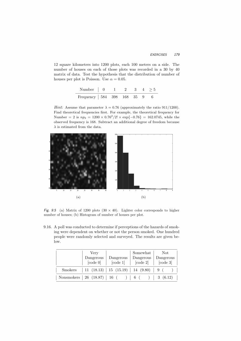
EXERCISES 179
12 square kilometers into 1200 plots, each 100 meters on a side. Thenumber of houses on each of those plots was recorded in a 30 by 40matrix of data. Test the hypothesis that the distribution of number ofhouses per plot is Poisson. Use α = 0.05.
Number 0 1 2 3 4 ≥ 5
Frequency 584 398 168 35 9 6
Hint: Assume that parameter λ = 0.76 (approximately the ratio 911/1200).
Find theoretical frequencies first. For example, the theoretical frequency for
Number = 2 is np2 = 1200 × 0.762/2! × exp−0.76 = 162.0745, while the
observed frequency is 168. Subtract an additional degree of freedom because
λ is estimated from the data.
5 10 15 20 25 30 35 40
5
10
15
20
25
300 1 2 3 4 5 6 7 8 9
0
100
200
300
400
500
600
(a) (b)
Fig. 9.5 (a) Matrix of 1200 plots (30 × 40). Lighter color corresponds to highernumber of houses; (b) Histogram of number of houses per plot.
9.16. A poll was conducted to determine if perceptions of the hazards of smok-ing were dependent on whether or not the person smoked. One hundredpeople were randomly selected and surveyed. The results are given be-low.
Very Somewhat NotDangerous Dangerous Dangerous Dangerous[code 0] [code 1] [code 2] [code 3]
Smokers 11 (18.13) 15 (15.19) 14 (9.80) 9 ( )
Nonsmokers 26 (18.87) 16 ( ) 6 ( ) 3 (6.12)

180 CATEGORICAL DATA
(a) Test the hypothesis that smoking status does not affect perceptionof the dangers of smoking at α = 0.05 (Five theoretical/expected fre-quencies are given in the parentheses).
(b) Observed frequencies of perceptions of danger [codes] for smokersare
[code 0] [code 1] [code 2] [code 3]
11 15 14 9
Are the codes coming from a discrete uniform distribution (i.e., eachcode is equally likely)? Use α = 0.01.
REFERENCES
Agresti, A. (1992), Categorical Data Analysis, 2nd ed, New York: Wiley.Benford, F. (1938), “The Law of Anomalous Numbers,” Proceedings of the
American Philosophical Society, 78, 551.Bickel, P. J., Hammel, E. A., and O‘Connell, J. W. (1975), “Sex Bias in
Graduate Admissions: Data from Berkeley,” Science, 187, 398-404.Cochran, W. G. (1950), “The Comparison of Percentages in Matched Sam-
ples,” Biometrika, 37, 256-266.Darwin, C. (1859), The Origin of Species by Means of Natural Selection, 1st
ed, London, UK: Murray.Deonier, R. C., Tavare, S., and Waterman, M. S. (2005), Computational
Genome Analysis: An Introduction. New York: Springer Verlag.Doucet, H., Shah, M. K., Cummings, T. L., and Kahm, M. J. (1999), “Com-
parison of Internal Medicine, Pediatric and Medicine/Pediatrics Appli-cants and Factors Influencing Career Choices,” Southern Medical Jour-nal, 92, 296-299.
Fisher, R. A. (1918), “The Correlation Between Relatives on the Supposi-tion of Mendelian Inheritance,” Philosophical Transactions of the RoyalSociety of Edinburgh, 52, 399433.
(1922), “On the Interpretation of Chi-Square from Contingency Ta-bles, and the Calculation of P,” Journal of the Royal Statistical Society,85, 87-94.
(1966), The Design of Experiments, 8th ed., Edinburgh, UK: Oliverand Boyd.

REFERENCES 181
Gilb, T., and Graham, D. (1993), Software Inspection, Reading, MA: Addison-Wesley.
Hill, T. (1998), “The First Digit Phenomenon,” American Scientist, 86, 358.Johnson, S., and Johnson, R. (1972), “Tonsillectomy History in Hodgkin’s
Disease,” New England Journal of Medicine, 287, 1122-1125.Liu, Z. (1992), “Smoking and Lung Cancer in China: Combined Analysis of
Eight Case-Control Studies,” International Journal of Epidemiology, 21,197-201.
Mantel, N., and Haenszel, W. (1959), “Statistical Aspects of the Analysis ofData from Retrospective Studies of Disease,” Journal of the NationalCancer Institute, 22, 719-729.
Matui, I. (1968), “Statistical Study of the Distribution of Scattered Villagesin Two Regions of the Tonami Plain, Toyama Prefecture,” in SpatialPatterns, Eds. Berry and Marble, Englewood Clifs, NJ: Prentice-Hall.
McNemar Q. (1947), “A Note on the Sampling Error of the Difference BetweenCorrelated Proportions or Percentages,” Psychometrika, 12, 153-157.
McWilliams, W. C. and Piotrowski , H. (2005) The World Since 1945: AHistory Of International Relations, Lynne Rienner Publishers.
(1960), “At Random: Sense and Nonsense,” American Psychologist,15, 295-300.
(1969), Psychological Statistics, 4th Edition, New York: Wiley.Pearson, K. (1900), “On the Criterion that a Given System of Deviations from
the Probable in the Case of a Correlated System of Variables is such thatit can be Reasonably Supposed to have Arisen from Random Sampling,”Philosophical Magazine, 50, 157 - 175.
Radelet, M. (1981), “Racial Characteristics and the Imposition of the DeathPenalty,” American Sociological Review, 46, 918-927.
Rasmussen, M. H., and Miller, L. A. (2004), “Echolocation and Social Signalsfrom White-beaked Dolphins, Lagenorhyncus albirostris, recorded in Ice-landic waters,” in Echolocation in Bats and Dolphins, ed. J.A.Thomas,et al, Chicago: University of Chicago Press.
Simonoff, J. S. (2003), Analyzing Categorical Data, New York: Springer Ver-lag.
Tanur J. M. ed. (1972), Statistics: A Guide to the Unknown, San Francisco:Holden-Day.
von Bortkiewicz, L. (1898), “Das Gesetz der Kleinen Zahlen,” Leipzig, Ger-many: Teubner.


10Estimating Distribution
Functions
The harder you fight to hold on to specific assumptions, the more likelythere’s gold in letting go of them.
John Seely Brown, former Chief Scientist at Xerox Corporation
10.1 INTRODUCTION
Let X1, X2, . . . , Xn be a sample from a population with continuous CDF F. InChapter 3, we defined the empirical (cumulative) distribution function (EDF)based on a random sample as
Fn(x) =1n
n∑
i=1
1(Xi ≤ x).
Because Fn(x), for a fixed x, has a sampling distribution directly related tothe binomial distribution, its properties are readily apparent and it is easy towork with as an estimating function.
The EDF provides a sound estimator for the CDF, but not through anymethodology that can be extended to general estimation problems in non-parametric statistics. For example, what if the sample is right truncated? Orcensored? What if the sample observations are not independent or identicallydistributed? In standard statistical analysis, the method of maximum like-lihood provides a general methodology for achieving inference procedures on
183

184 ESTIMATING DISTRIBUTION FUNCTIONS
unknown parameters, but in the nonparametric case, the unknown parameteris the function F (x) (or, equivalently, the survival function S(x) = 1−F (x)).Essentially, there are an infinite number of parameters. In the next section wedevelop a general formula for estimating the distribution function for non-i.i.d.samples. Specifically, the Kaplan-Meier estimator is constructed to estimateF (x) when censoring is observed in the data.
This theme continues in Chapter 11 where we introduce Density Estima-tion as a practical alternative to estimating the CDF. Unlike the cumulativedistribution, the density function provides a better visual summary of howthe random variable is distributed. Corresponding to the EDF, the empiricaldensity function is a discrete uniform probability distribution on the observeddata, and its graph doesn’t explain much about the distribution of the data.The properties of the more refined density estimators in Chapter 11 are not soeasily discerned, but it will give the researcher a smoother and visually moreinteresting estimator to work with.
In medical research, survival analysis is the study of lifetime distributionsalong with associated factors that affect survival rates. The time event mightbe an organism’s death, or perhaps the occurrence or recurrence of a diseaseor symptom.
10.2 NONPARAMETRIC MAXIMUM LIKELIHOOD
As a counterpart to the parametric likelihood, we define the nonparametriclikelihood of the sample X1, . . . , Xn as
L(F ) =n∏
i=1
(F (xi)− F (x−i )
), (10.1)
where F (x−i ) is defined as P (X < xi). This framework was first introducedby Kiefer and Wolfowitz (1956).
One serious problem with this definition is that L(F ) = 0 if F is continu-ous, which we might assume about the data. In order for L to be positive, theargument (F ) must put positive weight (or probability mass) on every one ofthe observations in the sample. Even if we know F is continuous, the non-parametric maximum likelihood estimator (NPMLE) must be non-continuousat the points of the data.
For a reasonable class of estimators, we consider nondecreasing functionsF that can have discrete and continuous components. Let pi = F (Xi:n) −F (Xi−1:n), where F (X0:n) is defined to be 0. We know that pj > 0 is required,or else L(F ) = 0. We also know that p1 + · · · + pn = 1, because if the sumis less than one, there would be probability mass assigned outside the setx1, . . . , xn. That would be impractical because if we reassigned that residualprobability mass (say q = 1− p1 − · · · − pn > 0) to any one of the values xi,

KAPLAN-MEIER ESTIMATOR 185
the likelihood L(F ) would increase in the term F (xi) − F (x−i ) = pi + q. Sothe NPMLE not only assigns probability mass to every observation, but onlyto that set, hence the likelihood can be equivalently expressed as
L(p1, . . . , pn) =n∏
i=1
pi,
which, under the constraint that∑
pi = 1, is the multinomial likelihood. TheNPMLE is easily computed as pi = 1/n, i = 1, . . . , n. Note that this solutionis quite intuitive – it places equal “importance” on all n of the observations,and it satisfies the constraint given above that
∑pi = 1. This essentially
proves the following theorem.
Theorem 10.1 Let X1, . . . , Xn be a random sample generated from F . Forany distribution function F0, the nonparametric likelihood L(F0) ≤ L(Fn),so that the empirical distribution function is the nonparametric maximumlikelihood estimator.
10.3 KAPLAN-MEIER ESTIMATOR
The nonparametric likelihood can be generalized to all sorts of observed datasets beyond a simple i.i.d. sample. The most commonly observed phenomenonoutside the i.i.d. case involves censoring. To describe censoring, we will con-sider X ≥ 0, because most problems involving censoring consist of lifetimemeasurements (e.g., time until failure).
(a) (b)
Fig. 10.1 Edward Kaplan (1920–2006) and Paul Meier (1924–).
Definition 10.1 Suppose X is a lifetime measurement. X is right censoredat time t if we know the failure time occurred after time t, but the actual time

186 ESTIMATING DISTRIBUTION FUNCTIONS
is unknown. X is left censored at time t if we know the failure time occurredbefore time t, but the actual time is unknown.
Definition 10.2 Type-I censoring occurs when n items on test are stoppedat a fixed time t0, at which time all surviving test items are taken off test andare right censored.
Definition 10.3 Type-II censoring occurs when n items (X1, . . . , Xn) ontest are stopped after a prefixed number of them (say, k ≤ n) have failed,leaving the remaining items to be right censored at the random time t = Xk:n.
Type I censoring is a common problem in drug treatment experimentsbased on human trials; if a patient receiving an experimental drug is knownto survive up to a time t but leaves the study (and humans are known to leavesuch clinical trials much more frequently than lab mice) the lifetime is rightcensored.
Suppose we have a sample of possibly right-censored values. We will as-sume the random variables represent lifetimes (or “occurrence times”). Thesample is summarized as (Xi, δi), i = 1, . . . , n, where Xi is a time mea-surement, and δi equals 1 if the Xi represents the lifetime, and equals 0 if Xi
is a (right) censoring time. If δi = 1, Xi contributes dF (xi) ≡ F (xi)−F (x−i )to the likelihood (as it does in the i.i.d. case). If δi = 0, we know only thatthe lifetime surpassed time Xi, so this event contributes 1 − F (xi) to thelikelihood. Then
L(F ) =n∏
i=1
(1− F (xi))1−δi (dF (xi))
δi . (10.2)
The argument about the NPMLE has changed from (10.1). In this case,no probability mass need be assigned to a value Xi for which δi = 0, be-cause in that case, dF (Xi) does not appear in the likelihood. Furthermore,the accumulated probability mass of the NPMLE on the observed data doesnot necessarily sum to one, because if the largest value of Xi is a censoredobservation, the term S(Xi) = 1 − F (Xi) will only be positive if probabilitymass is assigned to a point or interval to the right of Xi.
Let pi be the probability mass assigned to Xi:n. This new notation allowsfor positive probability mass (call it pn+1) that can be assigned to some arbi-trary point or interval after the last observation Xn:n. Let δi be the censoringindicator associated with Xi:n. Note that even though X1:n < · · · < Xn:n areordered, the set (δ1,. . . ,δn) is not necessarily so (δi is called a concomitant).
If δi = 1, the likelihood is clearly maximized by setting probability mass(say pi) on Xi:n. If δi = 0, some mass will be assigned to the right of Xi:n,which has interval probability pi+1 + · · · + pn+1. The likelihood based on

KAPLAN-MEIER ESTIMATOR 187
censored data is expressed
L(p1, . . . , pn+1) =n∏
i=1
pδii
n+1∑
j=i+1
pj
1−δi
.
Instead of maximizing the likelihood in terms of (p1, . . . , pn+1), it will proveto be much easier using the transformation
λi =pi∑n+1
j=i pj
.
This is a convenient one-to-one mapping where
n+1∑
j=i
pj =i−1∏
j=1
(1− λj), pi = λi
i−1∏
j=1
(1− λj).
The likelihood simplifies to
L(λ1, . . . , λn+1) =n∏
i=1
λi
i−1∏
j=1
(1− λj)
δi
i∏
j=1
(1− λj)
1−δi
=
(n∏
i=1
λiδi(1− λi)1−δi
)(n−1∏
i=1
(1− λi)n−i
)
=n∏
i=1
(λi
1− λi
)δi
(1− λi)n−i+1.
As a function of (λ1, . . . , λn+1), L is maximized at λi = δi/(n − i + 1), i =1, . . . , n + 1. Equivalently,
pi =δi
n− i + 1
i−1∏
j=1
(1− δj
n− j + 1
).
The NPMLE of the distribution function (denoted FKM (x)) can be expressedas a sum in pi. For example, at the observed order statistics, we see that
SKM (xi:n) ≡ 1− FKM (xi:n) =i∏
j=1
(1− 1
n− j + 1
)δj
(10.3)
=i∏
j=1
(1− δj
n− j + 1
).

188 ESTIMATING DISTRIBUTION FUNCTIONS
This is the Kaplan–Meier nonparametric estimator, developed by Kaplanand Meier (1958) for censored lifetime data analysis. It’s been one of themost influential developments in the past century; their paper is the most citedpaper in statistics (Stigler, 1994). E. L. Kaplan and Paul Meier never actuallymet during this time, but they both submitted their idea of the “productlimit estimator” to the Journal of the American Statistical Association atapproximately the same time, so their joint results were amalgamated throughletter correspondence.
For non-censored observations, the Kaplan-Meier estimator is identical tothe regular MLE. The difference occurs when there is a censored observation– then the Kaplan-Meier estimator takes the “weight” normally assigned tothat observation and distributes it evenly among all observed values to theright of the observation. This is intuitive because we know that the true valueof the censored observation must be somewhere to the right of the censoredvalue, but we don’t have any more information about what the exact valueshould be.
The estimator is easily extended to sets of data that have potential tiedvalues. If we define dj= number of failures at xj , mj = number of observationsthat had survived up to x−j , then
FKM (t) = 1−∏
xj≤t
(1− dj
mj
). (10.4)
Example 10.1 Muenchow (1986) tested whether male or female flowers (ofWestern White Clematis), were equally attractive to insects. The data inthe Table 10.15 represent waiting times (in minutes), which includes censoreddata. In MATLAB, use the function
KMcdfSM(x,y,j)
where x is a vector of event times, y is a vector of zeros (indicating censor)and ones (indicating failure), and j = 1 indicates the vector values ordered(j = 0 means the data will be sorted first).
Example 10.2 Data from Crowder et al. (1991) lists strength measurements(in coded units) for 48 pieces of weathered cord. Seven of the pieces of cordwere damaged and yielded strength measurements that are considered rightcensored. That is, because the damaged cord was taken off test, we knowonly the lower limit of its strength. In the MATLAB code below, vector datarepresents the strength measurements, and the vector censor indicates (witha zero) if the corresponding observation in data is censored.
>> data = [36.3,41.7,43.9,49.9,50.1,50.8,51.9,52.1,52.3,52.3,52.4,52.6,...

KAPLAN-MEIER ESTIMATOR 189
Table 10.15 Waiting Times for Insects to Visit Flowers
Male Flowers Female Flowers
1 9 27 1 19 571 9 27 2 23 592 9 30 4 23 672 11 31 4 26 714 11 35 5 28 754 14 36 6 29 75*5 14 40 7 29 78*5 14 43 7 29 816 16 54 8 30 90*6 16 61 8 32 94*6 17 68 8 35 967 17 69 9 35 96*7 18 70 14 37 100*8 19 83 15 39 102*8 19 95 18 43 105*8 19 102* 18 56
104*
0 20 40 60 80 100 1200
0.1
0.2
0.3
0.4
0.5
0.6
0.7
0.8
0.9
1
Fig. 10.2 Kaplan-Meier estimator for Waiting Times (solid line for male flowers,dashed line for female flowers).

190 ESTIMATING DISTRIBUTION FUNCTIONS
30 35 40 45 50 55 600
0.1
0.2
0.3
0.4
0.5
0.6
0.7
0.8
0.9
1
Fig. 10.3 Kaplan-Meier estimator cord strength (in coded units).
52.7,53.1,53.6,53.6,53.9,53.9,54.1,54.6,54.8,54.8,55.1,55.4,55.9,...
56.0,56.1,56.5,56.9,57.1,57.1,57.3,57.7,57.8,58.1,58.9,59.0,59.1,...
59.6,60.4,60.7,26.8,29.6,33.4,35.0,40.0,41.9,42.5];
>> censor=[ones(1,41),zeros(1,7)];
>> [kmest,sortdat,sortcen]= kmcdfsm(data’,censor’,0);
>> plot(sortdat,kmest,’k’);
The table below shows how the Kaplan-Meier estimator is calculated using theformula in (10.4) for the first 16 measurements, which includes seven censoredobservations. Figure 10.3 shows the estimated survival function for the cordstrength data.

KAPLAN-MEIER ESTIMATOR 191
Uncensored xj mj djmj−dj
mj1− FKM (xj)
26.8 48 0 1.000 1.00029.6 47 0 1.000 1.00033.4 46 0 1.000 1.00035.0 45 0 1.000 1.000
1 36.3 44 1 0.977 0.97740.0 43 0 1.000 0.977
2 41.7 42 1 0.976 0.95441.9 41 0 1.000 0.95442.5 40 0 1.000 0.954
3 43.9 39 1 0.974 0.9304 49.9 38 1 0.974 0.9055 50.1 37 1 0.973 0.8816 50.8 36 1 0.972 0.8567 51.9 35 1 0.971 0.8328 52.1 34 1 0.971 0.8079 52.3 33 2 0.939 0.758...
......
......
...
Example 10.3 Consider observing the lifetime of a series system. Recalla series system is a system of k ≥ 1 components that fails at the time thefirst component fails. Suppose we observe n different systems that are eachmade of ki identical components (i = 1, . . . , n) with lifetime distribution F .The lifetime data is denoted (x1, . . . , xn). Further suppose there is (random)right censoring, and δi = I(xi represents a lifetime measurement). How dowe estimate F?
If F (x) is continuous with derivative f(x), then the ith system’s survivalfunction is S(x)ki and its corresponding likelihood is
`i(F ) = ki (1− F (x))ki−1f(x).
It’s easier to express the full likelihood in terms of S(x) = 1− F (x):
L(S) =n∏
i=1
(ki (S(xi))
ki−1f(xi)
)δi (S(xi)ki
)1−δi,
where 1− δ indicates censoring.To make the likelihood more easy to solve, let’s examine the ordered sample
yi = xi:n so we observe y1 < y2 < · · · < yn. Let ki and δi represent the size ofthe series system and the censoring indicator for yi. Note that ki and δi areconcomitants of yi.

192 ESTIMATING DISTRIBUTION FUNCTIONS
The likelihood, now as a function of (y1, . . . , yn), is expressed
L(S) =n∏
i=1
(ki (S(yi))
ki−1f(yi)
)δi(S(yi)ki
)1−δi
∝n∏
i=1
f(yi)δiS(yi)ki−δi .
For estimating F nonparametrically, it is again clear that F (or S) will be astep-function with jumps occurring only at points of observed system failure.With this in mind, let Si = S(yi) and αi = Si/Si−1. Then fi = Si−1 − Si =∏i−1
r=1 αr(1− αi). If we let τj = kj + · · ·+ kn, the likelihood can be expressedsimply (see Exercise 10.4) as
L(S) =n∏
i=1
αiτi−δi (1− αi)
δi ,
and the nonparametric MLE for S(x), in terms of the ordered system lifetimes,is
S(yi) =i∏
r=1
(τr − δr
τr
).
Note the special case in which ki = 1 for all i, we end up with the Kaplan-Meier estimator.
10.4 CONFIDENCE INTERVAL FOR F
Like all estimators, F (x) is only as good as its measurement of uncertainty.Confidence intervals can be constructed for F (x) just as they are for regularparameters, but a typical inference procedure refers to a pointwise confidenceinterval about F (x) where x is fixed.
A simple, approximate 1− α confidence interval can be constructed usinga normal approximation
F (x)± z1−α/2σF ,
where σF is our estimate of the standard deviation of F (x). If we have ani.i.d. sample, F = Fn, and σ2
Fn= F (x)[1− F (x)]/n, so that
σ2F
= Fn(x)[1− Fn(x)]/n.
Recall that nFn(x) is distributed as binomial Bin(n, F (x)), and an exactinterval for F (x) can be constructed using the bounding procedure for the
PLUG-IN PRINCIPLE 193
binomial parameter p in Chapter 3.In the case of right censoring, a confidence interval can be based on the
Kaplan-Meier estimator, but the variance of FKM (x) does not have a sim-ple form. Greenwood’s formula (Greenwood, 1926), originally concocted forgrouped data, can be applied to construct a 1− α confidence interval for thesurvival function (S = 1− F ) under right censoring:
SKM (ti)± zα/2σKM (ti),
where
σ2KM (ti) = σ2(SKM (ti)) = SKM (ti)2
∑
tj≤ti
dj
mj(mj − dj).
It is important to remember these are pointwise confidence intervals, basedon fixed values of t in F (t). Simultaneous confidence bands are a more recentphenomenon and apply as a confidence statement for F across all values of tfor which 0 < F (t) < 1. Nair (1984) showed that the confidence bands by Halland Wellner (1980) work well in various settings, even though they are basedon large-sample approximations. An approximate 1 − α confidence band forS(t), for values of t less than the largest observed failure time, is
SKM (t)±√− 1
2nln
(α
2
)SKM (t)
(1 + σ2
KM (t)).
This interval is based on rough approximation for an infinite series, and aslightly better approximation can be obtained using numerical proceduressuggested in Nair (1984). Along with the Kaplan-Meier estimator of thedistribution of cord strength, Figure (10.3) also shows a 95% simultaneousconfidence band. The pointwise confidence interval at t=50 units is (0.8121,0.9934). The confidence band, on the other hand, is (0.7078, 1.0000). Notethat for small strength values, the band reflects a significant amount of un-certainty in FKM (x). See also the MATLAB procedure survBand.
10.5 PLUG-IN PRINCIPLE
With an i.i.d. sample, the EDF serves not only as an estimator for the underly-ing distribution of the data, but through the EDF, any particular parameterθ of the distribution can also be estimated. Suppose the parameter has aparticular functional relationship with the distribution function F :
θ = θ(F ).

194 ESTIMATING DISTRIBUTION FUNCTIONS
Examples are easy to construct. The population mean, for example, can beexpressed
µ = µ(F ) =∫ ∞
−∞xdF (x)
and variance is
σ2 = σ2(F ) =∫ ∞
−∞(x− µ)2dF (x).
As Fn is the sample analog to F , so θ(Fn) can serve as a sample-basedestimator for θ. This is the idea of the plug-in principle. The estimator forthe population mean:
µ = µ(Fn) =∫ ∞
−∞xdFn(x) =
∑x
xidFn(xi) = x.
Obviously, the plug-in principle is not necessary for simply estimating themean, but it is reassuring to see it produce a result that is consistent withstandard estimating techniques.
Example 10.4 The quantile xp can be expressed as a function of F : xp =infx :
∫∞x
dF (x) ≤ 1 − p. The sample equivalent is the value xp = infx :∫∞x
dFn(x) ≤ 1 − p. If F is continuous, then we have xp = F−1(p) andFn(xp) = p is solved uniquely. If F is discrete, xp is the smallest value of xfor which
n−1n∑
i=1
1(x ≤ xi) ≤ 1− p,
or, equivalently, the smallest order statistic xi:n for which i/n ≤ p, i.e.,(i + 1)/n > p. For example, with the flower data in Table 10.15, the me-dian waiting times are easily estimated as the smallest values (x) for whichFKM (x) ≤ 1/2, which are 16 (for the male flowers) and 29 (for the femaleflowers).
If the data are not i.i.d., the NPMLE F can be plugged in for F in θ(F ).This is a key selling point to the plug-in principle; it can be used to formulateestimators where we might have no set rule to estimate them. Depending onthe sample, F might be the EDF or the Kaplan-Meier estimator. The plug-intechnique is simple, and it will form a basis for estimating uncertainty usingre-sampling techniques in Chapter 15.
Example 10.5 To find the average cord strength from the censored data, forexample, it would be imprudent to merely average the data, as the censoredobservations represent a lower bound on the data, hence the true mean will be
SEMI-PARAMETRIC INFERENCE 195
underestimated. By using the plug in principle, we will get a more accurateestimate; the code below estimates the mean cord strength as 54.1946 (seealso the MATLAB m-file pluginmu. The sample mean, ignoring the censoringindicator, is 51.4438.
>> [cdfy svdata svcensor ] = kmcdfsm(vdata,vcensor,ipresorted);
>> if min(svdata)>0;
skm = 1-cdfy; %survival function
skm1 = [1, skm’];
svdata2 = [0 svdata’];
svdata3 = [svdata’ svdata(end)];
dx = svdata3 - svdata2;
mu_hat = skm1 *dx’;
else;
cdfy1 = [0, cdfy’];
cdfy2 = [cdfy’ 1];
df = cdfy2 - cdfy1;
svdata1 = [svdata’, 0];
mu_hat = svdata1 *df’;
end;
>> mu_hat
ans =
154.1946
10.6 SEMI-PARAMETRIC INFERENCE
The proportional hazards model for lifetime data relates two populations ac-cording to a common underlying hazard rate. Suppose r0(t) is a baselinehazard rate, where r(t) = f(t)/(1− F (t)). In reliability theory, r(t) is calledthe failure rate. For some covariate x that is observed along with the life-time, the positive function of Ψ(x) describes how the level of x can changethe failure rate (and thus the lifetime distribution):
r(t; x) = r0(t)Ψ(x).
This is termed a semi-parametric model because r0(t) is usually left un-specified (and thus a candidate for nonparametric estimation) where as Ψ(x) isa known positive function, at least up to some possibly unknown parameters.Recall that the CDF is related to the failure rate as
∫ x
−∞r(u)du ≡ R(u) = − ln S(x),
where S(x) = 1 − F (x) is called the survivor function. R(t) is called thecumulative failure rate in reliability and life testing. In this case, S0(t) is the

196 ESTIMATING DISTRIBUTION FUNCTIONS
baseline survivor function, and relates to the lifetime affected by Ψ(x) as
S(t;x) = S0(t)Ψ(x).
The most commonly used proportional hazards model used in survivalanalysis is called the Cox Model (named after Sir David Cox), which has theform
r(t; x) = r0(t)ex′β .
With this model, the (vector) parameter β is left unspecified and must beestimated. Suppose the baseline hazard function of two different populationsare related by proportional hazards as r1(t) = r0(t)λ and r2(t) = r0(t)θ. Thenif T1 and T2 represent lifetimes from these two populations,
P (T1 < T2) =λ
λ + θ.
The probability does not depend at all on the underlying baseline hazard (orsurvivor) function. With this convenient set-up, nonparametric estimation ofS(t) is possible through maximizing the nonparametric likelihood. Suppose npossibly right-censored observations (x1, . . . , xn) from F = 1−S are observed.Let ξi represent the number of observations at risk just before time xi. Then,if δi=1 indicates the lifetime was observed at xi,
L(β) =n∏
i=1
(ex′iβ
∑j∈ξi
ex′jβ
)δi
.
In general, the likelihood must be solved numerically. For a thorough studyof inference with a semi-parametric model, we suggest Statistical Models andMethods for Lifetime Data by Lawless. This area of research is paramount insurvival analysis.
Related to the proportional hazard model, is the accelerated lifetime modelused in engineering. In this case, the baseline survivor function S0(t) can rep-resent the lifetime of a test product under usage conditions. In an acceleratedlife test, and additional stress is put on the test unit, such as high or lowtemperature, high voltage, high humidity, etc. This stress is characterizedthrough the function Ψ(x) and the survivor function of the stressed test itemis
S(t; x) = S0(tΨ(x)).
Accelerated life testing is an important tool in product development, especiallyfor electronics manufacturers who produce gadgets that are expected to lastseveral years on test. By increasing the voltage in a particular way, as oneexample, the lifetimes can be shortened to hours. The key is how much faith

EMPIRICAL PROCESSES 197
the manufacturer has on the known acceleration function Ψ(x).In MATLAB, the Statistics Toolbox offers the routine coxphfit, which
computes Cox proportional hazards estimator for input data, much in thesame way the kmcdfsm computes the Kaplan-Meier estimator.
10.7 EMPIRICAL PROCESSES
If we express the sample as X1(ω), . . . , Xn(ω), we note that Fn(x) is both afunction of x and ω ∈ Ω. From this, the EDF can be treated as a randomprocess. The Glivenko-Cantelli Theorem from Chapter 3 states that the EDFFn(x) converges to F (x) (i) almost surely (as random variable, x fixed), and(ii) uniformly in x, (as a function of x with ω fixed). This can be expressedas:
P
(ω
∣∣∣∣ limn→∞
supx|Fn(x)− F (x)| = 0
)= 1.
Let W (x) be a standard Brownian motion process. It is defined as astochastic process for which W (0) = 0, W (t) ∼ N (0, t), W (t) has independentincrements, and the paths of W (t) are continuous. A Brownian Bridge isdefined as B(t) = W (t)− tW (1), 0 ≤ t ≤ 1. Both ends of a Brownian Bridge,B(0) and B(1), are tied to 0, and this property motivates the name. ABrownian motion W (x) has covariance function γ(t, s) = t ∧ s = min(t, s).This is because E(W (t)) = 0,Var(W (t)) = s, for s < t,Cov(W (t),W (s)) =Cov(W (s), (W (t)−W (s)) + W (s)) and W has independent increments.
Define the random process Bn(x) =√
n(Fn(x)− F (x)). This process con-verges to a Brownian Bridge Process, B(x), in the sense that all finite dimen-sional distributions of Bn(x) (defined by a selection of x1, . . . , xm) converge tothe corresponding finite dimensional distribution of a Brownian Bridge B(x).
Using this, one can show that a Brownian Bridge has mean zero and co-variance function γ(t, s) = t ∧ s − ts. If s < t, γ(s, t) = s(1 − t). For s < t,γ(s, t) = E(W (s)−sW (1))(W (t)− tW (1)) = · · · = s−st. Because the Brown-ian Bridge is a Gaussian process, it is uniquely determined by its second orderproperties. The covariance function γ(t, s) for the process
√n(Fn(t) − F (t))
is:
γ(t, s) = E[√
n(Fn(t)− F (t)) · √n(Fn(s)− F (s))]
= nE(Fn(t)− F (t))(Fn(s)− F (s)) =1n
(F (t) ∧ F (s)− F (t)F (s)).

198 ESTIMATING DISTRIBUTION FUNCTIONS
Proof:
Eγ(t, s) = E
(1n
∑
i
(1(Xi < t)− F (t)
)· 1
n
∑
j
(1(Xj < s)− F (s)
=1n2E
∑
i,j
(1(Xi < t)− F (t))(1(Xj < s)− F (s))
=1nE(1(X1 < t)− F (t))(1(X1 < s)− F (s))
=1nE [1(X1 < t ∧ s)− F (t)1(X1 < s)− F (s)1(X1 < t) + F (t)F (s)]
=1n
(F (t ∧ s)− F (t)F (s)).
This result is independent of F , as long as F is continuous, as the sampleX1, . . . , Xn could be transformed to uniform: Y1 = F (X1), . . . , Yn = F (Xn).Let Gn(t) be the empirical distribution based on Y1, . . . , Yn. For the uniformdistribution the covariance is γ(t, s) = t∧s−ts, which is exactly the correlationfunction of the Brownian Bridge. This leads to the following result:
Theorem 10.2 The random process√
n(Fn(x) − F (x)) converges in distri-bution to the Brownian Bridge process.
10.8 EMPIRICAL LIKELIHOOD
In Chapter 3 we defined the likelihood ratio based on the likelihood functionL(θ) =
∏f(xi; θ), where X1, . . . , Xn were i.i.d. with density function f(x; θ).
The likelihood ratio function
R(θ0) =L(θ0)
supθ L(θ)(10.5)
allows us to construct efficient tests and confidence intervals for the parameterθ. In this chapter we extend the likelihood ratio to nonparametric inference,although it is assumed that the research interest lies in some parameter θ =θ(F ), where F (x) is the unknown CDF.
The likelihood ratio extends naturally to nonparametric estimation. If wefocus on the nonparametric likelihood from the beginning of this chapter, froman i.i.d. sample of X1, . . . , Xn generated from F (x),
L(F ) =n∏
i=1
dF (xi) =n∏
i=1
(F (xi)− F (xi
−).

EMPIRICAL LIKELIHOOD 199
The likelihood ratio corresponding to this would be R(F ) = L(F )/L(Fn),where Fn is the empirical distribution function. R(F ) is called the empiricallikelihood ratio. In terms of F , this ratio doesn’t directly help us creatingconfidence intervals. All we know is that for any CDF F , R(F ) ≤ 1 andreaches its maximum only for F = Fn. This means we are considering onlyfunctions F that assign mass on the values Xi = xi, i = 1, . . . , n, and R isreduced to function of n − 1 parameters R(p1, . . . , pn−1) where pi = dF (xi)and
∑pi = 1.
It is more helpful to think of the problem in terms of an unknown pa-rameter of interest θ = θ(F ). Recall the plug-in principle can be applied toestimate θ with θ = θ(Fn). For example, with µ =
∫xdF (x) was merely the
sample mean, i.e.∫
xdFn(x) = x. We will focus on the mean as our firstexample to better understand the empirical likelihood.
Confidence Interval for the Mean. Suppose we have an i.i.d. sampleX1, . . . , Xn generated from an unknown distribution F (x). In the case µ(F ) =∫
xdF (x), define the set Cp(µ) on p = (p1, . . . , pn) as
Cp(µ) =
p :
n∑
i=1
pixi = µ, pi ≥ 0, i = 1, . . . , n,
n∑
i=1
pi = 1
.
The empirical likelihood associated with µ maximizes L(µ) over Cp(µ). Therestriction
∑pixi = µ is called the structural constraint. The empirical like-
lihood ratio (ELR) is this empirical likelihood divided by the unconstrainedNPMLE, which is just L(1/n, . . . , 1/n) = n−n. If we can find a set of solutionsto the empirical likelihood, Owen (1988) showed that
X2 = −2 log R(µ) = −2 log
(supp∈Cp
n∏
i=1
npi
)
is approximately distributed χ21 if µ is correctly specified, so a nonparametric
confidence interval for µ can be formed using the values of −2 log R(µ).MATLAB software is available to help: elm.m computes the empirical
likelihood for a specific mean, allowing the user to iterate to make a curvefor R(µ) and, in the process, construct confidence intervals for µ by solvingR(µ) = r0 for specific values of r0. Computing R(µ) is no simple matter;we can proceed with Lagrange multipliers to maximize
∑pixi subject to∑
pi = 1 and∑
ln(npi) = ln(r0). The best numerical optimization methodsare described in Chapter 2 of Owen (2001).
Example 10.6 Recall Exercise 6.2. Fuller et al. (1994) examined polishedwindow strength data to estimate the lifetime for a glass airplane window.The units are ksi (or 1,000 psi). The MATLAB code below constructs theempirical likelihood for the mean glass strength, which is plotted in Figure

200 ESTIMATING DISTRIBUTION FUNCTIONS
10.4 (a). In this case, a 90% confidence interval for µ is constructed by usingthe value of r0 so that −2 ln r0 < χ2
1(0.90) = 2.7055, or r0 > 0.2585. Theconfidence interval is computed as (28.78 ksi, 33.02 ksi).
>> x = [18.83 20.8 21.657 23.03 23.23 24.05 24.321 25.5 25.52 25.8 ...
26.69 26.77 26.78 27.05 27.67 29.9 31.11 33.2 33.73 33.76 33.89 ...
34.76 35.75 35.91 36.98 37.08 37.09 39.58 44.045 45.29 45.381 ];
>> n=size(x); i=1;
>> for mu=min(x):0.1:max(x)
R_mu=elm(x, mu,zeros(1,1), 100, 1e-7, 1e-9, 0 );
ELR_mu(i)=R_mu; Mu(i)=mu; i=i+1;
end
26 27 28 29 30 31 32 33 34 35 360
0.1
0.2
0.3
0.4
0.5
0.6
0.7
0.8
0.9
1
0 0.5 1 1.5 20
0.1
0.2
0.3
0.4
0.5
0.6
0.7
0.8
0.9
1
(a) (b)
Fig. 10.4 Empirical likelihood ratio as a function of (a) the mean and (b) the median(for different samples).
Owen’s extension of Wilk’s theorem for parametric likelihood ratios isvalid for other functions of F , including the variance, quantiles and more.To construct R for the median, we need only change the structural constraintfrom
∑pixi = µ to
∑pi sign(xi − x0.50) = 0.
Confidence Interval for the Median. In general, computing R(x) isdifficult. For the case of estimating a population quantile, however, the opti-mizing becomes rather easy. For example, suppose that n1 observations outof n are less than the population median x0.50 and n2 = n− n1 observationsare greater than x0.50. Under the constraint x0.50 = x0.50, the nonparametriclikelihood estimator assigns mass (2n1)−1 to each observation less than x0.50
and assigns mass (2n2)−1 to each observation to the right of x0.50, leaving us

EXERCISES 201
with
R(x0.50; n1, n2) =(
n
2n1
)n1(
n
2n2
)n2
.
Example 10.7 Figure 10.4(b), based on the MATLAB code below, shows theempirical likelihood for the median based on 30 randomly generated numbersfrom the exponential distribution (with µ=1 and x0.50 = − ln(0.5) = 0.6931).A 90% confidence interval for x0.50, again based on r0 > 0.2585, is (0.3035,0.9021).
>> n=30;
>> x=exprnd(1,1,n); y=sort(x);
>> n1=1:1:n; n2=n-n1;
>> R=((0.5*n./n1).^n1).*((0.5*n./n2).^n2);
>> stairs(y,R)
For general problems, computing the empirical likelihood is no easy matter,and to really utilize the method fully, more advanced study is needed. Thissection provides a modest introduction to let you know what is possible usingthe empirical likelihood. Students interested in further pursuing this methodare recommended to read Owen’s book.
10.9 EXERCISES
10.1. With an i.i.d. sample of n measurements, use the plug-in principle toderive an estimator for population variance.
10.2. Twelve people were interviewed and asked how many years they stayedat their first job. Three people are still employed at their first job andhave been there for 1.5, 3.0 and 6.2 years. The others reported thefollowing data for years at first job: 0.4, 0.9, 1.1, 1.9, 2.0, 3.3, 5.3, 5.8,14.0. Using hand calculations, compute a nonparametric estimator forthe distribution of T = time spent (in years) at first job. Verify yourhand calculations using MATLAB. According to your estimator, whatis the estimated probability that a person stays at their job for less thanfour years? Construct a 95% confidence interval for this estimate.
10.3. Using the estimator in Exercise 10.2, use the plug-in principle to com-pute the underlying mean number of years a person stays at their firstjob. Compare it to the faulty estimators based on using (a) only thenoncensored items and (b) using the censored times but ignoring thecensoring mechanism.
10.4. Consider Example 10.3, where we observe series-system lifetimes of aseries system. We observe n different systems that are each made of ki

202 ESTIMATING DISTRIBUTION FUNCTIONS
identical components (i = 1, . . . , n) with lifetime distribution F . Thelifetime data is denoted (x1, . . . , xn) and are possibly right censored.Show that if we let τj = kj + · · ·+ kn, the likelihood can be expressed as(10.5) and solve for the nonparametric maximum likelihood estimator.
10.5. Suppose we observe m different k-out-of-n systems and each systemcontains i.i.d. components (with distribution F ), and the ith systemcontains ni components. Set up the nonparametric likelihood functionfor F based on the n system lifetimes (but do not solve the likelihood).
10.6. Go to the link below to download survival times for 87 people with lupusnephritis. They were followed for 15+ or more years after an initialrenal biopsy. The duration variable indicates how long the patient hadthe disease before the biopsy; construct the Kaplan-Meier estimator forsurvival, ignoring the duration variable.
http://lib.stat.cmu.edu/datasets/lupus
10.7. Recall Exercise 6.3 based on 100 measurements of the speed of light inair. Use empirical likelihood to construct a 90% confidence interval forthe mean and median.
http://www.itl.nist.gov/div898/strd/univ/data/Michelso.dat
10.8. Suppose the empirical likelihood ratio for the mean was equal to R(µ)= µ1(0 ≤ µ ≤ 1)+ (2−µ)1(1 ≤ µ ≤ 2). Find a 95% confidence intervalfor µ.
10.9. The Receiver Operating Characteristic (ROC) curve is a statistical toolto compare diagnostic tests. Suppose we have a sample of measurements(scores) X1, . . . , Xn from a diseased population F (x), and a sample ofY1, . . . , Ym from a healthy population G(y). The healthy populationhas lower scores, so an observation is categorized as being diseased if itexceeds a given threshold value, e.g., if X > c. Then the rate of false-positive results would be P (Y > c). The ROC curve is defined as theplot of R(p) = F (G−1(p)). The ROC estimator can be computed usingthe plug-in principle:
R(p) = Fn(G−1m (p)).
A common test to see if the diagnostic test is effective is to see if R(p)remains well above 0.5 for 0 ≤ p ≤ 1. The Area Under the Curve (AUC)is defined as
AUC =∫ 1
0
R(p)dp.

REFERENCES 203
Show that AUC = P (X ≤ Y ) and show that by using the plug-inprinciple, the sample estimator of the AUC is equivalent to the Mann-Whitney two-sample test statistic.
REFERENCES
Brown, J. S. (1997), What It Means to Lead, Fast Company, 7. New York.Mansueto Ventures, LLC.
Cox, D. R. (1972), “Regression Models and Life Tables,” Journal of the RoyalStatistical Society (B), 34, 187-220.
Crowder, M. J., Kimber, A. C., Smith, R. L., and Sweeting, T. J. (1991),Statistical Analysis of Reliability Data, London, Chapman & Hall.
Fuller Jr., E. R., Frieman, S. W., Quinn, J. B., Quinn, G. D., and Carter, W.C. (1994), “Fracture Mechanics Approach to the Design of Glass AircraftWindows: A Case Study”, SPIE Proceedings, Vol. 2286, (Society ofPhoto-Optical Instrumentation Engineers (SPIE), Bellingham, WA).
Greenwood, M. (1926), “The Natural Duration of Cancer,” in Reports onPublic Health and Medical Subjects, 33, London: H. M. Stationery Office.
Hall, W. J., and Wellner, J. A. (1980), “Confidence Bands for a SurvivalCurve,” Biometrika, 67, 133-143.
Kaplan, E. L., and Meier, P. (1958), “Nonparametric Estimation from Incom-plete Observations,” Journal of the American Statistical Association, 53,457-481.
Kiefer, J., and Wolfowitz, J. (1956), “Consistency of the Maximum LikelihoodEstimator in the Presence of Infinitely Many Incidental Parameters,”Annals of Mathematical Statistics, 27, 887-906.
Lawless, J. F. (1982), Statistical Models and Methods for Lifetime Data, NewYork: Wiley.
Muenchow, G. (1986), “Ecological Use of Failure Time Analysis,” Ecology 67,246250.
Nair, V. N. (1984), “Confidence Bands for Survival Functions with CensoredData: A Comparative Study,” Technometrics, 26, 265-275.
Owen, A. B. (1988), “Empirical Likelihood Ratio Confidence Intervals for aSingle Functional,” Biometrika, 75, 237-249.
(1990), “Empirical Likelihood Confidence Regions,” Annals of Statis-tics, 18, 90-120.
(2001), Empirical Likelihood, Boca Raton, FL: Chapman & Hall/CRC.Stigler, S. M. (1994), “Citations Patterns in the Journals of Statistics and
Probability,” Statistical Science, 9, 94-108.

11Density Estimation
George McFly: Lorraine, my density has brought me to you.Lorraine Baines: What?George McFly: Oh, what I meant to say was...Lorraine Baines: Wait a minute, don’t I know you from somewhere?George McFly: Yes. Yes. I’m George, George McFly.I’m your density. I mean... your destiny.
From the movie Back to the Future, 1985
Probability density estimation goes hand in hand with nonparametric estima-tion of the cumulative distribution function discussed in Chapter 10. There,we noted that the density function provides a better visual summary of howthe random variable is distributed across its support. Symmetry, skewness,disperseness and unimodality are just a few of the properties that are ascer-tained when we visually scrutinize a probability density plot.
Recall, for continuous i.i.d. data, the empirical density function placesprobability mass 1/n on each of the observations. While the plot of theempirical distribution function (EDF) emulates the underlying distributionfunction, for continuous distributions the empirical density function takesno shape beside the changing frequency of discrete jumps of 1/n across thedomain of the underlying distribution – see Figure 11.2(a).
205

206 DENSITY ESTIMATION
Fig. 11.1 Playfair’s 1786 bar chart of wheat prices in England
11.1 HISTOGRAM
The histogram provides a quick picture of the underlying density by weightingfixed intervals according the their relative frequency in the data. Pearson(1895) coined the term for this empirical plot of the data, but its historygoes as far back as the 18th century. William Playfair (1786) is credited withthe first appearance of a bar chart (see Figure 11.1) that plotted the price ofwheat in England through the 17th and 18th centuries.
In MATLAB, the procedure hist(x) will create a histogram with ten binsusing the input vector x. Figure 11.2 shows (a) the empirical density functionwhere vertical bars represent Dirac’s point masses at the observations, and(b) a 10-bin histogram for a set of 30 generated N (0, 1) random variables.Obviously, by aggregating observations within the disjoint intervals, we geta better, smoother visual construction of the frequency distribution of thesample.
>> x = rand_nor(0,1,30,1);
>> hist(x)
>> histfit(x,1000)
The histogram represents a rudimentary smoothing operation that pro-vides the user a way of visualizing the true empirical density of the sample.Still, this simple plot is primitive, and depends on the subjective choices theuser makes for bin widths and number of bins. With larger data sets, wecan increase the number of bins while still keeping average bin frequency at areasonable number, say 5 or more. If the underlying data are continuous, thehistogram appears less discrete as the sample size (and number of bins) grow,but with smaller samples, the graph of binned frequency counts will not pickup the nuances of the underlying distribution.

KERNEL AND BANDWIDTH 207
−2 −1.5 −1 −0.5 0 0.5 1 1.5 2 2.50
0.1
0.2
0.3
0.4
0.5
0.6
0.7
0.8
0.9
1
−2 −1.5 −1 −0.5 0 0.5 1 1.5 2 2.50
1
2
3
4
5
6
(a) (b)
Fig. 11.2 Empirical “density” (a) and histogram (b) for 30 normal N (0, 1) variables.
The MATLAB function histfit(x,n) plots a histogram with n bins alongwith the best fitting normal density curve. Figure 11.3 shows how the appear-ance of continuity changes as the histogram becomes more refined (with morebins of smaller bin width). Of course, we do not have such luxury with smalleror medium sized data sets, and are more likely left to ponder the question ofunderlying normality with a sample of size 30, as in Figure 11.2(b).
>> x = rand_nor(0,1,5000,1);
>> histfit(x,10)
>> histfit(x,1000)
If you have no scruples, the histogram provides for you many opportunitiesto mislead your audience, as you can make the distribution of the data appeardifferently by choosing your own bin widths centered at a set of points arbi-trarily left to your own choosing. If you are completely untrustworthy, youmight even consider making bins of unequal length. That is sure to supporta conjectured but otherwise unsupportable thesis with your data, and mightjump-start a promising career for you in politics.
11.2 KERNEL AND BANDWIDTH
The idea of the density estimator is to spread out the weight of a singleobservation in a plot of the empirical density function. The histogram, then,is the picture of a density estimator that spreads the probability mass of eachsample item uniformly throughout the interval (i.e., bin) it is observed in.

208 DENSITY ESTIMATION
−4 −3 −2 −1 0 1 2 3 40
500
1000
1500
−4 −3 −2 −1 0 1 2 3 40
50
100
150
200
250
300
350
(a) (b)
Fig. 11.3 Histograms with normal fit of 5000 generated variables using (a) 10 binsand (b) 50 bins.
Note that the observations are in no way expected to be uniformly spread outwithin any particular interval, so the mass is not spread equally around theobservation unless it happens to fall exactly in the center of the interval.
In this chapter, we focus on the kernel density estimator that more fairlyspreads out the probability mass of each observation, not arbitrarily in a fixedinterval, but smoothly around the observation, typically in a symmetric way.With a sample X1, . . . , Xn, we write the density estimator
f(x) =1
nhn
n∑
i=1
K
(x− xi
hn
), (11.1)
for Xi = xi, i = 1, . . . , n. The kernel function K represents how the probabil-ity mass is assigned, so for the histogram, it is just a constant in any particu-lar interval. The smoothing function hn is a positive sequence of bandwidthsanalogous to the bin width in a histogram.
The kernel function K has five important properties –
1. K(x) ≥ 0 ∀x2. K(x) = K(−x) for x > 03.
∫K(u)du = 1
4.∫
uK(u)du = 05.
∫u2K(u)du = σ2
K < ∞.

KERNEL AND BANDWIDTH 209
−3 −2 −1 0 1 2 30
0.05
0.1
0.15
0.2
0.25
0.3
0.35
0.4
−2.5 −2 −1.5 −1 −0.5 0 0.5 1 1.5 2 2.50
0.05
0.1
0.15
0.2
0.25
0.3
0.35
0.4
0.45
(a) (b)
−2 −1.5 −1 −0.5 0 0.5 1 1.5 20
0.05
0.1
0.15
0.2
0.25
0.3
−2.5 −2 −1.5 −1 −0.5 0 0.5 1 1.5 2 2.50
0.05
0.1
0.15
0.2
0.25
0.3
0.35
(c) (d)
Fig. 11.4 (a) Normal, (b) Triangular, (c) Box, and (d) Epanechnickov kernel func-tions.
Figure 11.4 shows four basic kernel functions:
1. Normal (or Gaussian) kernel K(x) = φ(x),
2. Triangular kernel K(x) = c−2(c− |x|)1(−c < x < c), c > 0.
3. Epanechnickov kernel (described below).
4. Box kernel, K(x) = 1(−c < x < c)/(2c), c > 0.
While K controls the shape, hn controls the spread of the kernel. The accuracyof a density estimator can be evaluated using the mean integrated squarederror, defined as
MISE = E(∫
(f(x)− f(x))2dx
)
=∫
Bias2(f(x))dx +∫Var(f(x))dx. (11.2)
To find a density estimator that minimizes the MISE under the five mentionedconstraints, we also will assume that f(x) is continuous (and twice differen-tiable), hn → 0 and nhn → ∞ as n → ∞. Under these conditions it can be

210 DENSITY ESTIMATION
shown that
Bias(f(x)) =σ2
K
2f ′′(x) + O(h4
n) and
Var(f(x)
)=
f(x)R(K)nhn
+ O(n−1), (11.3)
where R(g) =∫
g(u)2du.We determine (and minimize) the MISE by our choice of hn. From the
equations in (11.3), we see that there is a tradeoff. Choosing hn to reducebias will increase the variance, and vice versa. The choice of bandwidth isimportant in the construction of f(x). If h is chosen to be small, the subtlenuances in the main part of the density will be highlighted, but the tail ofthe distribution will be unseemly bumpy. If h is chosen large, the tails of thedistribution are better handled, but we fail to see important characteristicsin the middle quartiles of the data.
By substituting in the bias and variance in the formula for (11.2), weminimize MISE with
h∗n =(
R(K)σ4
KR(f ′)
)1/5
n−1/5.
At this point, we can still choose K(x) and insert a “representative” densityfor f(x) to solve for the bandwidth. Epanechnickov (1969) showed that, uponsubstituting in f(x) = φ(x), the kernel that minimizes MISE is
KE(x) =
34 (1− x2) |x| ≤ 1
0 |x| > 1.
The resulting bandwidth becomes h∗n ≈ 1.06σn−1/5, where σ is the samplestandard deviation. This choice relies on the approximation of σ for f(x).Alternative approaches, including cross-validation, lead to slightly differentanswers.
Adaptive kernels were derived to alleviate this problem. If we use a moregeneral smoothing function tied to the density at xj , we could generalize thedensity estimator as
f(x) =1n
n∑
i=1
1hn,i
K
(x− xi
hn,i
). (11.4)
This is an advanced topic in density estimation, and we will not further pur-sue learning more about optimal estimators based on adaptive kernels here.We will also leave out details about estimator limit properties, and insteadpoint out that if hn is a decreasing function of n, under some mild regularityconditions, |f(x)−f(x)| P→ 0. For details and more advanced topics in density

KERNEL AND BANDWIDTH 211
8 10 12 14 16 18 20 220
0.05
0.1
0.15
0.2
0.25
0.3
0.35
8 10 12 14 16 18 20 220
0.05
0.1
0.15
0.2
0.25
0.3
0.35
8 10 12 14 16 18 20 220
0.05
0.1
0.15
0.2
0.25
0.3
0.35
(a) (b) (c)
Fig. 11.5 Density estimation for sample of size n=7 using various kernels: (all) Nor-mal, (a) Box, (b) Triangle, (c) Epanechnikov.
4 6 8 10 12 14 16 18 20 22 240
0.05
0.1
0.15
0.2
0.25
0.3
0.35
0.4
Fig. 11.6 Density estimation for sample of size n = 7 using various bandwidths.
estimation, see Silverman (1986) and Efromovich (1999).The (univariate) density estimator from MATLAB, called
ksdensity(data),
is illustrated in Figure 11.5 using a sample of seven observations. The defaultestimate is based on a normal kernel; to use another kernel, just enter ’box’,’triangle’, or ’epanechnikov’ (see code below). Figure 11.5 shows how the nor-mal kernel compares to the (a) box, (2) triangle and (c) epanechnikov kernels.Figure 11.6 shows the density estimator using the same data based on thenormal kernel, but using three different bandwidths. Note the optimal band-width (0.7449) can be found by allowing a third argument in the ksdensityoutput.
>> data1=[11,12,12.2,12.3,13,13.7,18];

212 DENSITY ESTIMATION
>> data2=[50,21,25.5,40.0,41,47.6,39];
>> [f1,x1]=ksdensity(data1,’kernel’,’box’);
>> plot(x1,f1,’-k’)
>> hold on
>> [f2,x2,band]=ksdensity(data1);
>> plot(x2,f2,’:k’)
>> band
band =
0.7449
>> [f1,x1]=ksdensity(data1,’width’,2);
>> plot(x1,f1,’--k’)
>> hold on
>> [f1,x1]=ksdensity(data1,’width’,1);
>> plot(x1,f1,’-k’)
>> [f1,x1]=ksdensity(data1,’width’,.5);
>> plot(x1,f1,’:k’)
Censoring. The MATLAB function ksdensity also handles right-censoreddata by adding an optional vector designating censoring. Although we willnot study the details about the way density estimators handle this problem,censored observations are treated in a way similar to nonparametric max-imum likelihood, with the weight assigned to the censored observation xc
being distributed proportionally to non-censored observations xt ≥ xc (seethe Kaplan-Meier estimator in Chapter 10). General weighting can also beincluded in the density estimation for ksdensity with an optional vector ofweights.
Example 11.1 Radiation Measurements. In some situations, the exper-imenter might prefer to subjectively decide on a proper bandwidth insteadof the objective choice of bandwidth that minimizes MISE. If outliers andsubtle changes in the probability distribution are crucial in the model, a morejagged density estimator (with a smaller bandwidth) might be preferred tothe optimal one. In Davies and Gather (1993), 2001 radiation measurementswere taken from a balloon at a height of 100 feet. Outliers occur when theballoon rotates, causing the balloon’s ropes to block direct radiation fromthe sun to the measuring device. Figure 11.7 shows two density estimates ofthe raw data, one based on a narrow bandwidth and the other more smoothdensity based on a bandwidth 10 times larger (0.01 to 0.1). Both densitiesare based upon a normal (Gaussian) kernel. While the more jagged estima-tor does show the mode and skew of the density as clearly as the smootherestimator, outliers are more easily discerned.
>> T=load(’balloondata.txt’);
>> T1=T(:,1); T2=T(:,2);
>> [f1,x1]=ksdensity(T1,’width’,.01);

EXERCISES 213
1.5 2 2.50
0.5
1
1.5
2
2.5
3
3.5
4
4.5
5
Fig. 11.7 Density estimation for 2001 radiation measurements using bandwidths band= 0.5 and band=0.05.
>> plot(x1,f1,’-k’)
>> hold on
>> [f2,x2]=ksdensity(T1,’width’,.1);
>> plot(x2,f2,’:k’)
11.2.1 Bivariate Density Estimators
To plot density estimators for bivariate data, a three-dimensional plot can beconstructed using MATLAB function kdfft2, noting that both x and y, thevectors designating plotting points for the density, must be of the same size.
In Figure 11.8, (univariate) density estimates are plotted for the sevenobservations [data1, data2]. In Figure 11.9, kdfft2 is used to producea two-dimensional density plot for the seven bivariate observations (coupledtogether).
11.3 EXERCISES
11.1. Which of the following serve as kernel functions for a density estimator?Prove your assertion one way or the other.
a. K(x) = 1(−1 < x < 1)/2,
b. K(x) = 1(0 < x < 1),

214 DENSITY ESTIMATION
10 12 14 16 18 20 220
0.05
0.1
0.15
0.2
0.25
0.3
0.35
30 35 40 45 50 550
0.02
0.04
0.06
0.08
0.1
0.12
0.14
(a) (b)
Fig. 11.8 (a) Univariate density estimator for first variable; (b) Univariate densityestimator for second variable.
c. K(x) = 1/x,
d. K(x) = 32 (2x + 1)(1− 2x) 1(− 1
2 < x < 12 ),
e. K(x) = 0.75(1− x2) 1(−1 < x < 1)
11.2. With a data set of 12, 15, 16, 20, estimate p∗ = P (observation is lessthan 15) using a density estimator based on a normal (Gaussian) ker-nel with hn =
√3/n. Use hand calculations instead of the MATLAB
function.
11.3. Generate 12 observations from a mixture distribution, where half of theobservations are from N (0, 1) and the other half are from N (1, 0.64).Use the MATLAB function ksdensity to create a density estimator.Change bandwidth to see its effect on the estimator. Repeat this pro-cedure using 24 observations instead of 12.
11.4. Suppose you have chosen kernel function K(x) and smoothing functionhn to construct your density estimator, where −∞ < K(x) < ∞. Whatshould you do if you encounter a right censored observation? For exam-ple, suppose the right-censored observation is ranked m lowest out of n,m ≤ n− 1.
11.5. Recall Exercise 6.3 based on 100 measurements of the speed of light inair. In that chapter we tested the data for normality. Use the samedata to construct a density estimator that you feel gives the best visualdisplay of the information provided by the data. What parameters didyou choose? The data can be downloaded from
http://www.itl.nist.gov/div898/strd/univ/data/Michelso.dat

REFERENCES 215
Fig. 11.9 Bivariate Density estimation for sample of size n = 7 using bandwidth =[2,2].
11.6. Go back to Exercise 10.6, where a link is provided to download right-censored survival times for 87 people with lupus nephritis. Construct adensity estimator for the survival, ignoring the duration variable.
http://lib.stat.cmu.edu/datasets/lupus
REFERENCES
Davies, L., and Gather, U. (1993), “The Identification of Multiple Outliers”(discussion paper), Journal of the American Statistical Association, 88,782-792.
Efromovich, S. (1999), Nonparametric Curve Estimation: Methods, Theoryand Applications, New York: Springer Verlag.
Epanechnikov, V. A. (1969), “Nonparametric Estimation of a MultivariateProbability Density,” Theory of Probability and its Applications, 14, 153-158.
Pearson, K. (1895), Contributions to the Mathematical Theory of EvolutionII, Philosophical Transactions of the Royal Society of London (A),186,

216 DENSITY ESTIMATION
343-414Playfair, W. (1786), Commercial and Political Atlas: Representing, by Copper-
Plate Charts, the Progress of the Commerce, Revenues, Expenditure, andDebts of England, during the Whole of the Eighteenth Century. London:Corry.
Silverman, B. (1986), Density Estimation for Statistics and Data Analysis,New York: Chapman & Hall.

12Beyond Linear
Regression
Essentially, all models are wrong, but some models are useful.
George Box, from Empirical Model-Building and Response Surfaces
Statistical methods using linear regression are based on the assumptionsthat errors, and hence the regression responses, are normally distributed.Variable transformations increase the scope and applicability of linear regres-sion toward real applications, but many modeling problems cannot fit in theconfines of these model assumptions.
In some cases, the methods for linear regression are robust to minor vi-olations of these assumptions. This has been shown in diagnostic methodsand simulation. In examples where the assumptions are more seriously vio-lated, however, estimation and prediction based on the regression model arebiased. Some residuals (measured difference between the response and themodel’s estimate of the response) can be overly large in this case, and wielda large influence on the estimated model. The observations associated withlarge residuals are called outliers, which cause error variances to inflate andreduce the power of the inferences made.
In other applications, parametric regression techniques are inadequate incapturing the true relationship between the response and the set of predictors.General “curve fitting” techniques for such data problems are introduced inthe next chapter, where the model of the regression is unspecified and notnecessarily linear.
In this chapter, we look at simple alternatives to basic least-squares re-
217

218 BEYOND LINEAR REGRESSION
gression. These estimators are constructed to be less sensitive to the outliersthat can affect regular regression estimators. Robust regression estimators aremade specifically for this purpose. Nonparametric or rank regression reliesmore on the order relations in the paired data rather than the actual datameasurements, and isotonic regression represents a nonparametric regressionmodel with simple constraints built in, such as the response being monotonewith respect to one or more inputs. Finally, we overview generalized linearmodels which although parametric, encompass some nonparametric methods,such as contingency tables, for example.
12.1 LEAST SQUARES REGRESSION
Before we introduce the less-familiar tools of nonparametric regression, wewill first review basic linear regression that is taught in introductory statisticscourses. Ordinary least-squares regression is synonymous with parametric re-gression only because of the way the errors in the model are treated. In thesimple linear regression case, we observe n independent pairs (Xi, Yi), wherethe linear regression of Y on X is the conditional expectation E(Y |X). A char-acterizing property of normally distributed X and Y is that the conditionalexpectation is linear, that is, E(Y |X) = β0 + β1X.
Standard least squares regression estimates are based on minimizing squarederrors
∑i(Yi − Yi)2 =
∑i(Yi − [β0 + β1Xi])2 with respect to the parameters
β1 and β0. The least squares solutions are
β1 =∑n
i=1(Xi − X)(Yi − Y )∑ni=1(Xi − X)2
(12.1)
=∑n
i=1(XiYi − nXY )∑ni=1 X2
i − nX2.
β0 = Y − β1X. (12.2)
This solution is familiar from elementary parametric regression. In fact,(β0, β1) are the MLEs of (β0, β1) in the case the errors are normally dis-tributed. But with the minimized least squares approach (treating the sum ofsquares as a “loss function”), no such assumptions were needed, so the modelis essentially nonparametric. However, in ordinary regression, the distribu-tional properties of β0 and β1 that are used in constructing tests of hypothesisand confidence intervals are pinned to assuming these errors are homogenousand normal.

RANK REGRESSION 219
12.2 RANK REGRESSION
The truest nonparametric method for modeling bivariate data is Spearman’scorrelation coefficient which has no specified model (between X and Y) andno assumed distributions on the errors. Regression methods, by their nature,require additional model assumptions to relate a random variable X to Yvia a function for the regression of E(Y |X). The technique discussed here isnonparametric except for the chosen regression model; error distributions areleft to be arbitrary. Here we assume the linear model
Yi = β0 + β1xi, i = 1, . . . , n
is appropriate and, using the squared errors as a loss function, we computeβ0 and β1 as in (12.2) and (12.1) as the least-squares solution.
Suppose we are interested in testing H0 that the population slope is equalto β10 against the three possible alternatives, H1 : β1 > β10, H1 : β1 < β10,H1 : β1 6= β10. Recall that in standard least-squares regression, the Pearsoncoefficient of linear correlation (ρ) between the Xs and Y s is connected to β1
via
ρ = β1 ·
√∑i X2
i − n(X)2√∑
i Y 2i − n(Y )2
.
To test the hypothesis about the slope, first calculate Ui = Yi−β10Xi, andfind the Spearman coefficient of rank correlation ρ between the Xis and theUis. For the case in which β10 = 0, this is no more than the standard Spear-man correlation statistic. In any case, under the assumption of independence,(ρ− ρ)
√n− 1 ∼ N (0, 1) and the tests against alternatives H1 are
Alternative p-value
H1 : β1 6= β10 p = 2P (Z ≥ |ρ|√n− 1)H1 : β1 < β10 p = P (Z ≤ ρ
√n− 1)
H1 : β1 > β10 p = P (Z ≥ ρ√
n− 1)
where Z ∼ N (0, 1). The table represents a simple nonparametric regressiontest based only on Spearman’s correlation statistic.
Example 12.1 Active Learning. Kvam (2000) examined the effect of ac-tive learning methods on student retention by examining students of an in-troductory statistics course eight months after the course finished. For a classtaught using an emphasis on active learning techniques, scores were comparedto equivalent final exam scores.
Exam 1 14 15 18 16 17 12 17 15 17 14 17 13 15 18 14Exam 2 14 10 11 8 17 9 11 13 12 13 14 11 11 15 9

220 BEYOND LINEAR REGRESSION
Scores for the first (x-axis) and second (y-axis) exam scores are plottedin Figure 12.1(a) for 15 active-learning students. In Figure 12.1(b), the solidline represents the computed Spearman correlation coefficient for Xi and Ui =Yi − β10Xi with β10 varying from -1 to 1. The dashed line is the p-valuecorresponding to the test H1 : β1 6= β10. For the hypothesis H0 : β1 ≥ 0versus H1 : β1 < 0, the p-value is about 0.12 (the p-value for the two-sidedtest, from the graph, is about 0.24).
Note that at β10 = 0.498, ρ is zero, and at β10 = 0, ρ = 0.387. The p-valueis highest at β10 = 0.5 and less than 0.05 for all values of β10 less than – 0.332.
>> n0=1000;
>> S=load(’activelearning.txt’);
>> trad1=S(:,1); trad2=S(:,2);
>> act1=S(:,3); act2=S(:,4);
>> trad=[trad1 trad2]; act=[act1 act2];
>> r=zeros(n0,1); p=zeros(n0,1); b=zeros(n0,1);
>> for i=1:n0
b(i)=(i-(n0/2))/(n0/2);
[r0 z0 p0]=spear(act1,act2-b(i)*act1);
r(i)=r0; p(i)=p0;
end
>> stairs(b,p,’:k’)
>> hold on
>> stairs(b,r,’-k’)
12 14 16 18
8
10
12
14
16
18
Test 1
Test 2
−1 −0.5 0 0.5 1−0.4
−0.2
0
0.2
0.4
0.6
0.8
1
Slope Parameter
(a) (b)
Fig. 12.1 (a) Plot of test #1 scores (during term) and test #2 scores (8 months after).(b) Plot of Spearman correlation coefficient (solid) and corresponding p-value (dotted)for nonparametric test of slope for −1 ≤ β10 ≤ 1.

ROBUST REGRESSION 221
12.2.1 Sen-Theil Estimator of Regression Slope
Among n bivariate observations, there are(n2
)different pairs (Xi, Yi) and
(Xj , Yj), i 6= j. For each pair (Xi, Yi) and (Xj , Yj), 1 ≤ i < j ≤ n we find thecorresponding slope
Sij =Yj − Yi
Xj −Xi.
Compared to ordinary least-squares regression, a more robust estimator of theslope parameter β1 is
β1 = medianSij , 1 ≤ i < j ≤ n.
Corresponding to the least-squares estimate, let
β0 = medianY − β1medianX.
Example 12.2 If we take n = 20 integers 1, . . . , 20 as our set of predictorsX1, . . . , X20, let Y be 2X + ε where ε is a standard normal variable. Next, wechange both Y1 and Y20 to be outliers with value 20 and compare the ordinaryleast squares regression with the more robust nonparametric method in Figure12.2.
−5 0 5 10 15 20 25−5
0
5
10
15
20
25
30
35
40
45
Fig. 12.2 Regression: Least squares (dotted) and nonparametric (solid).
12.3 ROBUST REGRESSION
“Robust” estimators are ones that retain desired statistical properties evenwhen the assumptions about the data are slightly off. Robust linear regres-

222 BEYOND LINEAR REGRESSION
sion represents a modeling alternative to regular linear regression in the casethe assumptions about the error distributions are potentially invalid. In thesimple linear case, we observe n independent pairs (Xi, Yi), where the linearregression of Y on X is the conditional expectation E(Y |X) = β0 + β1X.
For rank regression, the estimator of the regression slope is considered tobe robust because no single observation (or small group of observations) willhave an significant influence on estimated model; the regression slope picksout the median slope out of the
(n2
)different pairings of data points.
One way of measuring robustness is the regression’s breakdown point, whichis the proportion of bad data needed to affect the regression adversely. Forexample, the sample mean has a breakdown point of 0, because a single obser-vation can change it by an arbitrary amount. On the other hand, the samplemedian has a breakdown point of 50 percent. Analogous to this, ordinaryleast squares regression has a breakdown point of 0, while some of the robusttechniques mentioned here (e.g., least-trimmed squares) have a breakdownpoint of 50 percent.
There is a big universe of robust estimation. We only briefly introducesome robust regression techniques here, and no formulations or derivationsare given. A student who is interested in learning more should read an intro-ductory textbook on the subject, such as Robust Statistics by Huber (1981)..
12.3.1 Least Absolute Residuals Regression
By squaring the error as a measure of discrepancy, the least-squares regressionis more influenced by outliers than a model based on, for example, absolutedeviation errors:
∑i |Yi − Yi|, which is called Least Absolute Residuals Re-
gression. By minimizing errors with a loss function that is more “forgiving”to large deviations, this method is less influenced by these outliers. In placeof least-squares techniques, regression coefficients are found from linear pro-gramming.
12.3.2 Huber Estimate
The concept of robust regression is based on a more general class of estimates(β0, β1) that minimize the function
n∑
i=1
ψ(Yi − Yi)σ
,
where ψ is a loss function and σ is a scale factor. If ψ(x) = x2, we have regularleast-squares regression, and if ψ(x) = |x|, we have least absolute residuals

ROBUST REGRESSION 223
regression. A general loss function introduced by Huber (1975) is
ψ(x) =
x2 |x| < c2c|x| − c2 |x| > c.
Depending on the chosen value of c > 0, ψ(x) uses squared-error loss for smallerrors, but the loss function flattens out for larger errors.
12.3.3 Least Trimmed Squares Regression
Least Trimmed Squares (LTS) is another robust regression technique proposedby Rousseeuw (1985) as a robust alternative to ordinary least squares regres-sion. Within the context of the linear model yi = β′xi, i = 1, . . . , n, the LTSestimator is represented by the value of β that minimizes
∑hi=1 ri:n. Here, xi
is a px1 vector and ri:n is the ith order statistic from the squared residualsri = (yi − β′xi)2 and h is a trimming constant (n/2 ≤ h ≤ n) chosen so thatthe largest n− h residuals do not affect the model estimate. Rousseeuw andLeroy (1987) showed that the LTS estimator has its highest level of robustnesswhen h = bn/2c + b(p + 1)/2c. While choosing h to be low leads to a morerobust estimator, there is a tradeoff of robustness for efficiency.
12.3.4 Weighted Least Squares Regression
For some data, one can improve model fit by including a scale factor (weight)in the deviation function. Weighted least squares minimizes
n∑
i=1
wi(yi − yi)2,
where wi are weights that determine how much influence each response willhave on the final regression. With the weights in the model, we estimate β inthe linear model with
β = (X ′WX)−1X ′Wy,
where X is the design matrix made up of the vectors xi, y is the responsevector, and W is a diagonal matrix of the weights w1, . . . , wn. This canbe especially helpful if the responses seem not to have constant variances.Weights that counter the effect of heteroskedasticity, such as
wi = m
(m∑
i=1
(yi − y)2)−1
,

224 BEYOND LINEAR REGRESSION
work well if your data contain a lot of replicates; here m is the number ofreplicates at yi. To compute this in MATLAB, the function lscov computesleast-squares estimates with known covariance; for example, the output of
lscov(A,B,W)
returns the weighted least squares solution to the linear system AX = B withdiagonal weight matrix X.
12.3.5 Least Median Squares Regression
The least median of squares (LMS) regression finds the line through the datathat minimizes the median (rather than the mean) of the squares of the errors.While the LMS method is proven to be robust, it cannot be easily solved likea weighted least-squares problem. The solution must be solved by searchingin the space of possible estimates generated from the data, which is usuallytoo large to do analytically. Instead, randomly chosen subsets of the data arechosen so that an approximate solution can be computed without too muchtrouble. The MATLAB function
lmsreg(y,X)
computes the LMS for small or medium sized data sets.
Example 12.3 Star Data. Data from Rousseeuw and Leroy (1987), p. 27,Table 3, are given in all panels of Figure 12.3 as a scatterplot of temperatureversus light intensity for 47 stars. The first variable is the logarithm ofthe effective temperature at the surface of the star (Te) and the second oneis the logarithm of its light intensity (L/L0). In sequence, the four panelsin Figure 12.3 show plots of the bivariate data with fitted regressions basedon (a) Least Squares, (b) Least Absolute Residuals, (c) Huber Loss & LeastTrimmed Squares, and (d) Least Median Squares. Observations far away frommost of the other observations are called leverage points; in this example, onlythe Least Median Squares approach works well because of the effect of theleverage points.
>> stars = load(’stars.txt’); n = size(stars,1);
>> X = [ones(n,1) stars(:,2)]; y = stars(:,3);
>> bols = X\y; [ignore,idx] = sort(stars(:,2));
>> plot(stars(:,2),stars(:,3),’o’,stars(idx,2),...
X(idx,:)*bols,’-.’ )
legend(’Data’,’OLS’)
>> %
>> % Least Absolute Deviation
>> blad = medianregress(stars(:,2),stars(:,3));
>> plot(stars(:,2),stars(:,3),’o’,stars(idx,2),...
X(idx,:)*bols,’-.’,stars(idx,2),X(idx,:)*blad,’-.’)
legend(’Data’,’OLS’,’LAD’);

ROBUST REGRESSION 225
3.4 3.6 3.8 4 4.2 4.4 4.6 4.8 53.5
4
4.5
5
5.5
6
6.5
3.4 3.6 3.8 4 4.2 4.4 4.6 4.8 53.5
4
4.5
5
5.5
6
6.5
(a) (b)
3.4 3.6 3.8 4 4.2 4.4 4.6 4.8 53.5
4
4.5
5
5.5
6
6.5
3.4 3.6 3.8 4 4.2 4.4 4.6 4.8 51
2
3
4
5
6
7
(c) (d)
Fig. 12.3 Star data with (a) OLS Regression, (b) Least Absolute Deviation, (c) HuberEstimation and Least Trimmed Squares, (d) Least Median Squares.
>> %
>> % Huber Estimation
>> k = 1.345; % tuning parameters in Huber’s weight function
>> wgtfun = @(e) (k*(abs(e)>k)-abs(e).*(abs(e)>k))./abs(e)+1;
>> % Huber’s weight function
>> wgt = rand(length(y),1); % Initial Weights
>> b0 = lscov(X,y,wgt);
>> res = y - X*b0; % Raw Residuals
>> res = res/mad(res)/0.6745; % Standardized Residuals
>> m = 30;
>> for i=1:m
wgt = wgtfun(res);
% Compute the weighted estimate using these weights
bhuber = lscov(X,y,wgt);
if all((bhuber-b0)<.01*b0)% Stop with convergence
return;
else
res = y - X*bhuber;
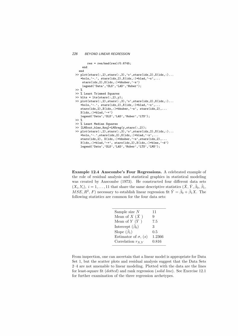
226 BEYOND LINEAR REGRESSION
res = res/mad(res)/0.6745;
end
end
>> plot(stars(:,2),stars(:,3),’o’,stars(idx,2),X(idx,:)...
*bols,’-.’, stars(idx,2),X(idx,:)*blad,’-x’,...
stars(idx,2),X(idx,:)*bhuber,’-s’)
legend(’Data’,’OLS’,’LAD’,’Huber’);
>> %
>> % Least Trimmed Squares
>> blts = lts(stars(:,2),y);
>> plot(stars(:,2),stars(:,3),’o’,stars(idx,2),X(idx,:)...
*bols,’-.’, stars(idx,2),X(idx,:)*blad,’-x’,...
stars(idx,2),X(idx,:)*bhuber,’-s’, stars(idx,2),...
X(idx,:)*blad,’-+’)
legend(’Data’,’OLS’,’LAD’,’Huber’,’LTS’);
>> %
>> % Least Median Squares
>> [LMSout,blms,Rsq]=LMSreg(y,stars(:,2));
>> plot(stars(:,2),stars(:,3),’o’,stars(idx,2),X(idx,:)...
*bols,’-.’,stars(idx,2),X(idx,:)*blad,’-x’,...
stars(idx,2), X(idx,:)*bhuber,’-s’,stars(idx,2),...
X(idx,:)*blad,’-+’, stars(idx,2),X(idx,:)*blms,’-d’)
legend(’Data’,’OLS’,’LAD’,’Huber’,’LTS’,’LMS’);
Example 12.4 Anscombe’s Four Regressions. A celebrated example ofthe role of residual analysis and statistical graphics in statistical modelingwas created by Anscombe (1973). He constructed four different data sets(Xi, Yi), i = 1, . . . , 11 that share the same descriptive statistics (X, Y , β0, β1,
MSE,R2, F ) necessary to establish linear regression fit Y = β0 + β1X. Thefollowing statistics are common for the four data sets:
Sample size N 11Mean of X (X ) 9Mean of Y (Y ) 7.5Intercept (β0) 3Slope (β1) 0.5Estimator of σ, (s) 1.2366Correlation rX,Y 0.816
From inspection, one can ascertain that a linear model is appropriate for DataSet 1, but the scatter plots and residual analysis suggest that the Data Sets2–4 are not amenable to linear modeling. Plotted with the data are the linesfor least-square fit (dotted) and rank regression (solid line). See Exercise 12.1for further examination of the three regression archetypes.

ISOTONIC REGRESSION 227
DataSet 1
X 10 8 13 9 11 14 6 4 12 7 5Y 8.04 6.95 7.58 8.81 8.33 9.96 7.24 4.26 10.84 4.82 5.68
DataSet 2
X 10 8 13 9 11 14 6 4 12 7 5Y 9.14 8.14 8.74 8.77 9.26 8.10 6.13 3.10 9.13 7.26 4.74
DataSet 3
X 10 8 13 9 11 14 6 4 12 7 5Y 7.46 6.77 12.74 7.11 7.81 8.84 6.08 5.39 8.15 6.42 5.73
DataSet 4
X 8 8 8 8 8 8 8 19 8 8 8Y 6.58 5.76 7.71 8.84 8.47 7.04 5.25 12.50 5.56 7.91 6.89
12.4 ISOTONIC REGRESSION
In this section we consider bivariate data that satisfy an order or restrictionin functional form. For example, if Y is known to be a decreasing function ofX, a simple linear regression need only consider values of the slope parameterβ1 < 0. If we have no linear model, however, there is nothing in the empiricalbivariate model to ensure such a constraint is satisfied. Isotonic regressionconsiders a restricted class of estimators without the use of an explicit regres-sion model.
Consider the dental study data in Table 12.16, which was used to illustrateisotonic regression by Robertson, Wright, and Dykstra (1988). The data areoriginally from a study of dental growth measurements of the distance (mm)from the center of the pituitary gland to the pterygomaxillary fissure (referringto the bone in the lower jaw) for 11 girls between the age of 8 and 14. Itis assumed that PF increases with age, so the regression of PF on age isnondecreasing. But it is also assumed that the relationship between PF andage is not necessarily linear. The means (or medians, for that matter) arenot strictly increasing in the PF data. Least squares regression does yield anincreasing function for PF: Y = 0.065X + 21.89, but the function is nearlyflat and not altogether well-suited to the data.
For an isotonic regression, we impose some order of the response as afunction of the regressors.
Definition 12.1 If the regressors have a simple order x1 ≤ · · · ≤ xn, afunction f is isotonic with respect to x if f(x1) ≤ · · · ≤ f(xn). For ourpurposes, isotonic will be synonymous with monotonic. For some function gof X, we call the function g∗ an isotonic regression of g with weights w if and

228 BEYOND LINEAR REGRESSION
4 6 8 10 12 14 16 18 204
5
6
7
8
9
10
11
12
13
14
4 6 8 10 12 14 16 18 202
4
6
8
10
12
14
(a) (b)
4 6 8 10 12 14 16 18 205
6
7
8
9
10
11
12
13
4 6 8 10 12 14 16 18 204
5
6
7
8
9
10
11
12
13
14
(c) (d)
Fig. 12.4 Anscombe’s regressions: LS and Robust.
only if g∗ is isotonic (i.e., retains the necessary order) and minimizes
n∑
i=1
w(xi) (g(xi)− f(xi))2 (12.3)
in the class of all isotonic functions f .
12.4.1 Graphical Solution to Regression
We can create a simple graph to show how the isotonic regression can besolved. Let Wk =
∑ki=1 w(xi) and Gk =
∑ki=1 g(xi)w(xi). In the example,
the means are ordered, so f(xi) = µi and wi = ni, the number of observationsat each age group. We let g be the set of PF means, and the plot of Wk
versus Gk, called the cumulative sum diagram (CSD), shows that the empirical

ISOTONIC REGRESSION 229
Table 12.16 Size of Pituitary Fissure for Subjects of Various Ages.
Age 8 10 12 14
PF 21,23.5,23 24,21,25 21.5,22,19 23.5,25
Mean 22.50 23.33 20.83 24.25PAVA 22.22 22.22 22.22 24.25
relationship between PF and age is not isotonic.Define G∗ to be the greatest convex minorant (GCM) which represents the
largest convex function that lies below the CSD. You can envision G∗ as ataut string tied to the left most observation (W1, G1) and pulled up and underthe CSD, ending at the last observation. The example in Figure 12.5(a) showsthat the GCM for the nine observations touches only four of them in forminga tight convex bowl around the data.
0
50
100
150
200
250
3 6 9 14
W(k)
G(k
)
(a) (b)
Fig. 12.5 (a) Greatest convex minorant based on nine observations. (b) Greatestconvex minorant for dental data.
The GCM represents the isotonic regression. The reasoning follows below(and in the theorem that follows). Because G∗ is convex, it is left differentiableat Wi. Let g∗(xi) be the left-derivative of G∗ at Wi. If the graph of the GCMis under the graph of CSD at Wi, the slopes of the GCM to the left and rightof Wi remain the same, i.e., if G∗(Wi) < Gi, then g∗(xi+1) = g∗(xi). Thisillustrates part of the intuition of the following theorem, which is not provenhere (see Chapter 1 of Robertson, Wright, and Dykstra (1988)).

230 BEYOND LINEAR REGRESSION
Theorem 12.1 For function f in (12.3), the left-hand derivative g∗ of thegreatest convex minorant is the unique isotonic regression of g on f . That is,if f is isotonic on X, then
n∑
i=1
w(xi) (g(xi)− f(xi))2 ≥
n∑
i=1
w(xi) (g(xi)− g∗(xi))2 +
n∑
i=1
w(xi) (g∗(xi)− f(xi))2.
Obviously, this graphing technique is going to be impractical for problemsof any substantial size. The following algorithm provides an iterative way ofsolving for the isotonic regression using the idea of the GCM.
12.4.2 Pool Adjacent Violators Algorithm
In the CSD, we see that if g(xi−1) > g(xi) for some i, then g is not isotonic.To construct an isotonic g∗, take the first such pair and replace them withthe weighted average
gi = gi−1 =w(xi−1)g(xi−1) + w(xi)g(xi)
w(xi−1) + w(xi).
Replace the weights w(xi) and w(xi−1) with w(xi) + w(xi−1). If thiscorrection (replacing g with g) makes the regression isotonic, we are finished.Otherwise, we repeat this process with until an isotonic is set. This is calledthe Pool Adjacent Violators Algorithm or PAVA.
Example 12.5 In Table 12.16, there is a decrease in PF between ages 10 and12, which violates the assumption that pituitary fissure increases in age. Oncewe replace the PF averages by the average over both age groups (22.083), westill lack monotonicity because the PF average for girls of age 8 was 22.5.Consequently, these two categories, which now comprise three age groups, areaveraged. The final averages are listed in the bottom row of Table 12.16
12.5 GENERALIZED LINEAR MODELS
Assume that n (p + 1)-tuples (yi, x1i, x2i, . . . , xpi), i = 1, . . . , n are observed.The values yi are responses and components of vectors xi = (x1i, x2i, . . . , xpi)′
are predictors. As we discussed at the beginning of this chapter, the standardtheory of linear regression considers the model
Y = Xβ + ε, (12.4)

GENERALIZED LINEAR MODELS 231
where Y = (Y1, . . . , Yn) is the response vector, X = (1n x1 x2 . . . xp) isthe design matrix (1n is a column vector of n 1’s), and ε is vector of errorsconsisting of n i.i.d normal N (0, σ2) random variables. The variance σ2 iscommon for all Yis and independent of predictors ir the order of observation.The parameter β is a vector of (p + 1) parameters in the linear relationship,
EYi = x′iβ = β0 + β1x1i + . . . βpxpi.
(a) (b)
Fig. 12.6 (a) Peter McCullagh and (b) John Nelder.
The term generalized linear model (GLM) refers to a large class of models,introduced by Nelder and Wedderburn (1972) and popularized by McCullaghand Nelder (1994), Figure 12.6 (a-b). In a canonical GLM, the response vari-able Yi is assumed to follow an exponential family distribution with mean µi,which is assumed to be a function of x′iβ. This dependence can be nonlin-ear, but the distribution of Yi depends on covariates only through their linearcombination, ηi = x′iβ, called a linear predictor. As in the linear regression,the epithet linear refers to being linear in parameters, not in the explanatoryvariables. Thus, for example, the linear combination
β0 + β1 x1 + β2 x22 + β3 log(x1 + x2) + β4 x1 · x2,
is a perfect linear predictor. What is generalized in model given in (12.4) bya GLM?
The three main generalizations concern the distributions of responses, thedependence of response on linear predictor, and variance if the error.
1. Although Yis remain independent, their (common) distribution is gen-eralized. Instead of normal, their distribution is selected from the ex-ponential family of distributions (see Chapter 2). This family is quiteversatile and includes normal, binomial, Poisson, negative binomial, andgamma as special cases.

232 BEYOND LINEAR REGRESSION
2. In the linear model (12.4) the mean of Yi, µi = EYi was equal to x′iβ.The mean µi in GLM depends on the predictor ηi = x′iβ as
g(µi) = ηi (= x′iβ). (12.5)
The function g is called the link function. For the model (12.4), the linkis the identity function.
3. The variance of Yi was constant (12.4). In GLM it may not be constantand could depend on the mean µi.
Models and inference for categorical data, traditionally a non-parametrictopic, are unified by a larger class of models which are parametric in natureand that are special cases of GLM. For example, in contingency tables, thecell counts Nij could be modeled by multinomial Mn(n, pij) distribution.The standard hypothesis in contingency tables is concerning the independenceof row/column factors. This is equivalent to testing H0 : pij = αiβj for someunknown αi and βj such that
∑i αi =
∑j βj = 1.
The expected cell count ENij = npij , so that under H0 becomes ENij =nαiβj , by taking the logarithm of both sides one obtains
logENij = log n + log αi + log βj
= const + ai + bj ,
for some parameters ai and bj . Thus, the test of goodness of fit for this modellinear and additive in parameters a and b, is equivalent to the test of theoriginal independence hypothesis H0 in the contingency table. More of suchexamples will be discussed in Chapter 18.
12.5.1 GLM Algorithm
The algorithms for fitting generalized linear models are robust and well es-tablished (see Nelder and Wedderburn (1972) and McCullagh and Nelder(1994)). The maximum likelihood estimates of β can be obtained using iter-ative weighted least-squares (IWLS).
(i) Given vector µ(k), the initial value of the linear predictor η(k) is formedusing the link function, and components of adjusted dependent variate(working response), z
(k)i , can be formed as
z(k)i = η
(k)i +
(yi − µ
(k)i
) (dη
dµ
)(k)
i
,
where the derivative is evaluated at the the available kth value.

GENERALIZED LINEAR MODELS 233
(ii) The quadratic (working) weights, W(k)i , are defined so that
1
W(k)i
=(
dη
dµ
)2
i
V(k)i ,
where V is the variance function evaluated at the initial values.
(iii) The working response z(k) is then regressed onto the covariates xi, withweights W
(k)i to produce new parameter estimates, β(k+1). This vector
is then used to form new estimates
η(k+1) = X ′β(k+1) and µ(k+1) = g−1(η(k+1)).
We repeat iterations until changes become sufficiently small. Startingvalues are obtained directly from the data, using µ(0) = y, with occa-sional refinements in some cases (for example, to avoid evaluating log 0when fitting a log-linear model with zero counts).
By default, the scale parameter should be estimated by the mean deviance,n−1
∑ni=1 D(yi, µ), from p. 44 in Chapter 3, in the case of the normal and
gamma distributions.
12.5.2 Links
In the GLM the predictors for Yi are summarized as the linear predictorηi = x′iβ. The link function is a monotone differentiable function g such thatηi = g(µi), where µi = EYi. We already mentioned that in the normal caseµ = η and the link is identity, g(µ) = µ.
Example 12.6 For analyzing count data (e.g., contingency tables), the Pois-son model is standardly assumed. As µ > 0, the identity link is inappropriatebecause η could be negative. However, if µ = eη, then the mean is alwayspositive, and η = log(µ) is an adequate link.
A link is called natural if it is connecting θ (the natural parameter in theexponential family of distributions) and µ. In the Poisson case,
f(y|λ) = exp y log λ− (λ + log y!) ,
µ = λ and θ = log µ. Accordingly, the log is the natural link for the Poissondistribution.
Example 12.7 For the binomial distribution,
f(y|π) =(
n
y
)πy(1− π)n−y
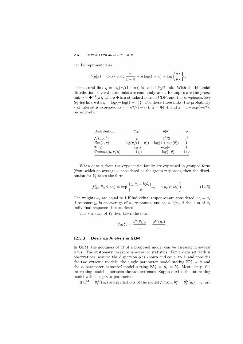
234 BEYOND LINEAR REGRESSION
can be represented as
f(y|π) = exp
y logπ
1− π+ n log(1− π) + log
(n
y
).
The natural link η = log(π/(1 − π)) is called logit link. With the binomialdistribution, several more links are commonly used. Examples are the probitlink η = Φ−1(π), where Φ is a standard normal CDF, and the complementarylog-log link with η = log− log(1− π). For these three links, the probabilityπ of interest is expressed as π = eη/(1+eη), π = Φ(η), and π = 1−exp−eη,respectively.
Distribution θ(µ) b(θ) φ
N (µ, σ2) µ θ2/2 σ2
Bin(1, π) log(π/(1− π)) log(1 + exp(θ)) 1P(λ) log λ exp(θ) 1Gamma(µ, ν/µ) −1/µ − log(−θ) 1/ν
When data yi from the exponential family are expressed in grouped form(from which an average is considered as the group response), then the distri-bution for Yi takes the form
f(yi|θi, φ, ωi) = exp
yiθi − b(θi)φ
ωi + c(yi, φ, ωi)
. (12.6)
The weights ωi are equal to 1 if individual responses are considered, ωi = ni
if response yi is an average of ni responses, and ωi = 1/ni if the sum of ni
individual responses is considered.The variance of Yi then takes the form
VarYi =b′′(θi)φ
ωi=
φV (µi)ωi
.
12.5.3 Deviance Analysis in GLM
In GLM, the goodness of fit of a proposed model can be assessed in severalways. The customary measure is deviance statistics. For a data set with nobservations, assume the dispersion φ is known and equal to 1, and considerthe two extreme models, the single parameter model stating EYi = µ andthe n parameter saturated model setting EYi = µi = Yi. Most likely, theinteresting model is between the two extremes. Suppose M is the interestingmodel with 1 < p < n parameters.
If θMi = θMi (µi) are predictions of the model M and θSi = θSi (yi) = yi are

GENERALIZED LINEAR MODELS 235
the predictions of the saturated model, then the deviance of the model M is
DM = 2n∑
i=1
[(yiθ
Si (yi)− b(θSi ))− (yiθ
Mi − b(θMi ))
].
When the dispersion φ is estimated and different than 1, the scaled devianceof the model M is defined as D∗
M = DM/φ.
Example 12.8 For yi ∈ 0, 1 in the binomial family,
D = 2n∑
1=1
yi log
(yi
yi
)+ (ni − yi) log
(ni − yi
ni − yi
).
• Deviance is minimized at saturated model S. Equivalently, the log-likelihood `S = `(y|y) is the maximal log-likelihood with the data y.
• The scaled deviance D∗M is asymptotically distributed as χ2
n−p. Signif-icant deviance represents the deviation from a good model fit.
• If a model K with q parameters, is a subset of model M with p param-eters (q < p), then
D∗K −D∗
Mφ
∼ χ2p−q.
Residuals are critical for assessing the model (recall four Anscombe’s re-gressions on p. 226). In standard normal regression models, residuals are cal-culated simply as yi − µi, but in the context of GLMs, both predicted valuesand residuals are more ambiguous. For predictions, it is important to distin-guish the scale: (i) predictions on the scale of η = x′iβ and (ii) predictions onthe scale of the observed responses yi for which EYi = g−1(ηi).
Regarding residuals, there are several approaches. Response residuals aredefined as ri = yi− g−1(ηi) = yi− θi. Also, the deviance residuals are definedas
rDi = sign(yi − µi)
√di,
where di are observation specific contributions to the deviance D.Deviance residuals are ANOVA-like decompositions,
∑
i
(rDi )2 = D,
thus testably assessing the contribution of each observation to the model de-viance. In addition, the deviance residuals increase with yi − µi and aredistributed approximately as standard normals, irrespectively of the type ofGLM.
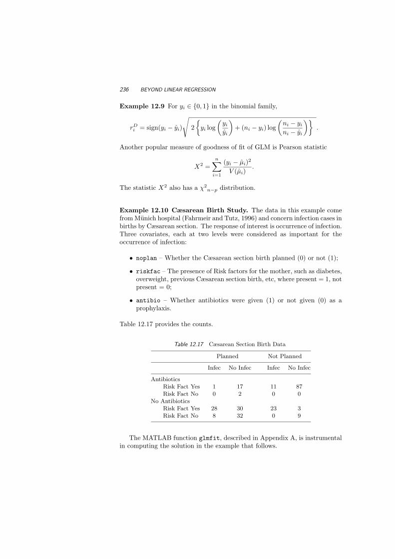
236 BEYOND LINEAR REGRESSION
Example 12.9 For yi ∈ 0, 1 in the binomial family,
rDi = sign(yi − yi)
√2
yi log
(yi
yi
)+ (ni − yi) log
(ni − yi
ni − yi
).
Another popular measure of goodness of fit of GLM is Pearson statistic
X2 =n∑
i=1
(yi − µi)2
V (µi).
The statistic X2 also has a χ2n−p distribution.
Example 12.10 Cæsarean Birth Study. The data in this example comefrom Munich hospital (Fahrmeir and Tutz, 1996) and concern infection cases inbirths by Cæsarean section. The response of interest is occurrence of infection.Three covariates, each at two levels were considered as important for theoccurrence of infection:
• noplan – Whether the Cæsarean section birth planned (0) or not (1);
• riskfac – The presence of Risk factors for the mother, such as diabetes,overweight, previous Cæsarean section birth, etc, where present = 1, notpresent = 0;
• antibio – Whether antibiotics were given (1) or not given (0) as aprophylaxis.
Table 12.17 provides the counts.
Table 12.17 Cæsarean Section Birth Data
Planned Not Planned
Infec No Infec Infec No Infec
AntibioticsRisk Fact Yes 1 17 11 87Risk Fact No 0 2 0 0
No AntibioticsRisk Fact Yes 28 30 23 3Risk Fact No 8 32 0 9
The MATLAB function glmfit, described in Appendix A, is instrumentalin computing the solution in the example that follows.

EXERCISES 237
>> infection = [1 11 0 0 28 23 8 0];
>> total = [18 98 2 0 58 26 40 9];
>> proportion = infection./total;
>> noplan = [0 1 0 1 0 1 0 1];
>> riskfac = [1 1 0 0 1 1 0 0];
>> antibio = [1 1 1 1 0 0 0 0];
>> [logitCoef2,dev] = glmfit([noplan’ riskfact’ antibio’],...
[infection’ total’],’binomial’,’logit’);
>> logitFit = glmval(logitCoef2,[noplan’ riskfact’ antibio’],’logit’);
>> plot(1:8, proportion,’ks’, 1:8, logitFit,’ko’);
The scaled deviance of this model is distributed as χ23. The number
of degrees of freedom is equal to 8 (n) vector infection minus 5 for thefive estimated parameters, β0, β1, β2, β3, φ. The deviance dev=11 is significant,yielding a p-value of 1 - chi2cdf(11,3)=0.0117. The additive model (withno interactions) in MATLAB yields
logP (infection)
P (no infection)= β0 + β1 noplan + β2 riskfac + β3 antibio.
The estimators of (β0, β1, β2, β3) are, respectively, (−1.89, 1.07, 2.03,−3.25).The interpretation of the estimators is made more clear if we look at the oddsratio
P (infection)
P (no infection)= eβ0 · eβ1noplan · eβ2riskfac · eβ3antibio.
At the value antibio = 1, the antibiotics have the odds ratio of infection/noinfection. This increases by the factor exp(−3.25) = 0.0376, which is a de-crease of more than 25 times. Figure 12.7 shows the observed proportionsof infections for 16 combinations of covariates (noplan, riskfac, antibio)marked by squares and model-predicted probabilities for the same combi-nations marked by circles. We will revisit this example in Chapter 18; seeExample 18.5.
12.6 EXERCISES
12.1. Using robust regression, find the intercept and slope β0 and β1 for eachof the four data sets of Anscombe (1973) from p. 226. Plot the ordinaryleast squares regression along with the rank regression estimator of slope.Contrast these with one of the other robust regression techniques. Forwhich set does β1 differ the most from its LS counterpart β1 = 0.5?Note that in the fourth set, 10 out of 11 Xs are equal, so one should useSij = (Yj−Yi)/(Xj−Xi+ε) to avoid dividing by 0. After finding β0 andβ1, are they different than β0 and β1? Is the hypothesis H0 : β1 = 1/2rejected in a robust test against the alternative H1 : β1 < 1/2, for Data

238 BEYOND LINEAR REGRESSION
1 2 3 4 5 6 7 80
0.1
0.2
0.3
0.4
0.5
0.6
0.7
0.8
Fig. 12.7 Cæsarean Birth Infection observed proportions (squares) and model predic-tions (circles). The numbers 1-8 on the x-axis correspond to following combinationsof covariates (noplan, riskfac, antibio): (0,1,1), (1,1,1), (0,0,1), (1,0,1), (0,1,0),(1,1,0), (0,0,0), and (1,0,0).
Set 3? Note, here β10 = 1/2.
12.2. Using the PF data in Table 12.16, compute a median squares regressionand compare it to the simple linear regression curve.
12.3. Using the PF data in Table 12.16, compute a nonparametric regressionand test to see if β10 = 0.
12.4. Consider the Gamma(α, α/µ) distribution. This parametrization wasselected so that Ey = µ. Identify θ and φ as functions of α and µ.Identify functions a, b and c.
Hint: The density can be represented as
exp−α log µ− αy
µ+ α log(α) + (α− 1) log y − log(Γ(α))
12.5. The zero-truncated Poisson distribution is given by
f(y|λ) =λj
j!(eλ − 1), j = 1, 2, . . .
Show that f is a member of exponential family with canonical parameterlog λ.

EXERCISES 239
12.6. Dalziel, Lagen and Thurston (1941) conducted an experiment to assessthe effect of small electrical currents on farm animals, with the eventualgoal of understanding the effects of high-voltage powerlines on livestock.The experiment was carried out with seven cows, and six shock intensi-ties: 0, 1, 2, 3, 4, and 5 milliamps (note that shocks on the order of 15milliamps are painful for many humans). Each cow was given 30 shocks,five at each intensity, in random order. The entire experiment was thenrepeated, so each cow received a total of 60 shocks. For each shockthe response, mouth movement, was either present or absent. The dataas quoted give the total number of responses, out of 70 trials, at eachshock level. We ignore cow differences and differences between blocks(experiments).
Current Number of Number of Proportion of(milliamps) Responses Trials Responses
0 0 70 0.0001 9 70 0.1292 21 70 0.3003 47 70 0.6714 60 70 0.8575 63 70 0.900
Propose a GLM in which the probability of a response is modeled witha value of Current (in milliamps) as a covariate.
12.7. Bliss (1935) provides a table showing the number of flour beetles killedafter five hours exposure to gaseous carbon disulphide at various concen-trations. Propose a logistic regression model with a Dose as a covariate.
Table 12.18 Bliss Beetle Data
Dose Number of Number(log10 CS2 mgl−1) Beetles Killed
1.6907 59 61.7242 60 131.7552 62 181.7842 56 281.8113 63 521.8369 59 531.8610 62 611.8839 60 60
According to your model, what is the probability that a beetle will bekilled if a dose of gaseous carbon disulphide is set to 1.8?

240 BEYOND LINEAR REGRESSION
REFERENCES
Anscombe, F. (1973), “Graphs in Statistical Analysis,” American Statistician,27, 17-21.
Bliss, C. I. (1935), “The Calculation of the Dose-Mortality Curve,” Annals ofApplied Biology, 22, 134-167.
Dalziel, C, F. Lagen, J. B., and Thurston, J. L. (1941), “Electric Shocks,”Transactions of IEEE, 60, 1073-1079.
Fahrmeir, L., and Tutz, G. (1994), Multivariate Statistical Modeling Based onGeneralized Linear Models, New York: Springer Verlag
Huber, P. J. (1973), “Robust Regression: Asymptotics, Conjectures, andMonte Carlo,” Annals of Statistics, 1, 799-821.
(1981), Robust Statistics, New York: Wiley.Kvam, P. H. (2000), “The Effect of Active Learning Methods on Student
Retention in Engineering Statistics,” American Statistician, 54, 2, 136-140.
Lehmann, E. L. (1998), Nonparametrics: Statistical Methods Based on Ranks,New Jersey: Prentice-Hall.
McCullagh, P., and Nelder, J. A. (1994), Generalized Linear Models, 2nd ed.London: Chapman & Hall.
Nelder, J. A., and Wedderburn, R. W. M. (1972), “Generalized Linear Mod-els,” Journal of the Royal Statistical Society, Ser. A, 135, 370-384.
Robertson, T., Wright, T. F., and Dykstra, R. L. (1988), Order RestrictedStatistical Inference, New York: Wiley.
Rousseeuw, P. J. (1985), “Multivariate Estimation with High BreakdownPoint,” in Mathematical Statistics and Applications B , Eds. W. Gross-mann et al., pp. 283-297, Dordrecht: Reidel Publishing Co.
Rousseeuw P. J. and Leroy A. M. (1987). Robust Regression and OutlierDetection. New York: Wiley.

13Curve Fitting Techniques
“The universe is not only queerer than we imagine, it is queerer thanwe can imagine”
J.B.S. Haldane (Haldane’s Law)
In this chapter, we will learn about a general class of nonparametric regres-sion techniques that fit a response curve to input predictors without makingstrong assumptions about error distributions. The estimators, called smooth-ing functions, actually can be smooth or bumpy as the user sees fit. The finalregression function can be made to bring out from the data what is deemedto be important to the analyst. Plots of a smooth estimator will give the usera good sense of the overall trend between the input X and the response Y .However, interesting nuances of the data might be lost to the eye. Such detailswill be more apparent with less smoothing, but a potentially noisy and jaggedcurve plotted made to catch such details might hide the overall trend of thedata. Because no linear form is assumed in the model, this nonparametricregression approach is also an important component of nonlinear regression,which can also be parametric.
Let (X1, Y1), . . . , (Xn, Yn) be a set of n independent pairs of observationsfrom the bivariate random variable (X, Y ). Define the regression functionm(x) as E(Y |X = x). Let Yi = m(Xi) + εi, i = 1, . . . , n when εi’s areerrors with zero mean and constant variance. The estimators here are locally
241
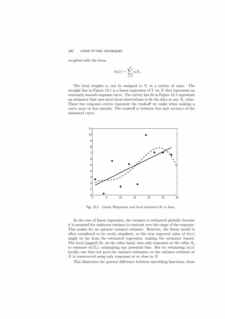
242 CURVE FITTING TECHNIQUES
weighted with the form
m(x) =n∑
i=1
aiYi.
The local weights ai can be assigned to Yi in a variety of ways. Thestraight line in Figure 13.1 is a linear regression of Y on X that represents anextremely smooth response curve. The curvey line fit in Figure 13.1 representsan estimator that uses more local observations to fit the data at any Xi value.These two response curves represent the tradeoff we make when making acurve more or less smooth. The tradeoff is between bias and variance of theestimated curve.
0 5 10 15 20 25 300
1
2
3
4
5
6
7
8
9
10
11
Fig. 13.1 Linear Regression and local estimator fit to data.
In the case of linear regression, the variance is estimated globally becauseit is assumed the unknown variance is constant over the range of the response.This makes for an optimal variance estimate. However, the linear model isoften considered to be overly simplistic, so the true expected value of m(x)might be far from the estimated regression, making the estimator biased.The local (jagged) fit, on the other hand, uses only responses at the value Xi
to estimate m(Xi), minimizing any potential bias. But by estimating m(x)locally, one does not pool the variance estimates, so the variance estimate atX is constructed using only responses at or close to X.
This illustrates the general difference between smoothing functions; those

KERNEL ESTIMATORS 243
that estimate m(x) using points only at x or close to it have less bias andhigh variance. Estimators that use data from a large neighborhood of x willproduce a good estimate of variance but risk greater bias. In the next sections,we feature two different ways of defining the local region (or neighborhood) ofa design point. At an estimation point x, kernel estimators use fixed intervalsaround x such as x± c0 for some c0 > 0. Nearest neighbor estimators use thespan produced by a fixed number of design points that are closest to x.
13.1 KERNEL ESTIMATORS
Let K(x) be a real-valued function for assigning local weights to the linearestimator, that is,
y(x) =∑
K
(x− xi
h
)yi.
If K(u) ∝ 1(|u| ≤ 1) then a fitted curve based on K(x−xi
h ) will estimatem(x) using only design points within h units of x. Usually it is assumed that∫
RK(x)dx = 1, so any bounded probability density could serve as a kernel.
Unlike kernel functions used in density estimation, now K(x) also can takenegative values, and in fact such unrestricted kernels are needed to achieveoptimal estimators in the asymptotic sense. An example is the beta kerneldefined as
K(x) =1
B(1/2, γ + 1)(1− x2
)γ1(|x| ≤ 1), γ = 0, 1, 2 . . . (13.1)
With the added parameter γ, the beta-kernel is remarkably flexible. Forγ = 0, the beta kernel becomes uniform. If γ = 1 we get the Epanechikovkernel, γ = 2 produces the biweight kernel, γ = 3 the triweight, and so on(see Figure 11.4 on p. 209). For γ large enough, the beta kernel is close theGaussian kernel
K(x) =1√
2πσ2e−
x2σ2 ,
with σ2 = 1/(2γ + 3), which is the variance of densities from (13.1). Forexample, if γ = 10, then
∫ 1
−1
(K(x)− σ−1φ(x/σ)
)2dx ≈ 0.00114, where σ =
1/√
2γ + 3. Define a scaling coefficient h so that
Kh(x) =1h
K(x
h
), (13.2)
where h is the associated bandwidth. By increasing h, the kernel functionspreads weight away from its center, thus giving less weight to those datapoints close to x and sharing the weight more equally with a larger group of

244 CURVE FITTING TECHNIQUES
design points. A family of beta kernels and the Epanechikov kernel are givenin Figure 13.2.
−1.5 −1 −0.5 0 0.5 1 1.50
0.2
0.4
0.6
0.8
1
1.2
1.4
1.6
1.8
−10 −5 0 5 10−0.05
0
0.05
0.1
0.15
0.2
0.25
0.3
0.35
0.4
(a) (b)
Fig. 13.2 (a) A family of symmetric beta kernels; (b) K(x) = 12
exp−|x|/√2sin(|x|/√2− π/4).
13.1.1 Nadaraya-Watson Estimator
Nadaraya (1964) and Watson (1964) independently published the earliest re-sults on for smoothing functions (but this is debateable), and the Nadaraya-Watson Estimator (NWE) of m(x) is defined as
m(x) =∑n
i=1 Kh(Xi − x)Yi∑ni=1 Kh(Xi − x)
. (13.3)
For x fixed, the value θ that minimizes
n∑
i=1
(Yi − θ)2Kh(Xi − x), (13.4)
is of the form∑n
i=1 aiYi. The Nadaraya-Watson estimator is the minimizer of(13.4) with ai = Kh(Xi − x)/
∑ni=1 Kh(Xi − x).
Although several competing kernel-based estimators have been derivedsince, the NWE provided the basic framework for kernel estimators, includinglocal polynomial fitting which is described later in this section. The MATLABfunction
nada wat(x0, X, Y, bw)

KERNEL ESTIMATORS 245
0 0.2 0.4 0.6 0.8 1−1.5
−1
−0.5
0
0.5
1
1.5
2datah=0.015h=0.030h=0.060
Fig. 13.3 Nadaraya-Watson Estimators for different values of bandwidth.
computes the Nadaraya-Watson kernel estimate at x = x0. Here, (X,Y ) areinput data, and bw is the bandwidth.
Example 13.1 Noisy pairs (Xi, Yi), i = 1, . . . , 200 are generated in the fol-lowing way:
>> x=sort(rand(1,200));
>> y=sort(rand(1,200));
>> y=sin(4*pi*y)+0.3*randn(1,200);
Three bandwidths are selected h = 0.015, 0.030, and 0.060. The threeNadaraya-Watson Estimators are shown in Figure 13.3. As expected, the es-timators constructed with the larger bandwidths appear smoother than thosewith smaller bandwidths.
13.1.2 Gasser-Muller Estimator.
The Gasser-Muller estimator proposed in 1979 uses areas of the kernel for theweights. Suppose Xi are ordered, X1 ≤ X2 · · · ≤ Xn. Let X0 = −∞ andXn+1 = ∞ and define midpoints si = (Xi + Xi+1)/2. Then
m(x) =n∑
i=1
Yi
∫ si
si−1
Kh(u− x)du. (13.5)
The Gasser-Muller estimator is the minimizer of (13.4) with the weights ai =∫ si
si−1Kh(u− x)du.

246 CURVE FITTING TECHNIQUES
13.1.3 Local Polynomial Estimator
Both Nadaraya-Watson and Gasser-Muller estimators are local constant fitestimators, that is, they minimize weighted squared error
∑ni=1(Yi−θ)2ωi for
different values of weights ωi. Assume that for z in a small neighborhood ofx the function m(z) can well be approximated by a polynomial of order p :
m(z) ≈p∑
j=0
βj(z − x)j
where βj = m(j)(x)/j!. Instead of minimizing (13.4), the local polynomial(LP) estimator minimizes
n∑
i=1
Yi −
p∑
j=0
βj(Xi − x)j
2
Kh(Xi − x) (13.6)
over β1, . . . , βp. Assume, for a fixed x, βj , j = 0, . . . , p minimize (13.6). Then,m(x) = β0, and an estimator of jth derivative of m is
m(j)(x) = j!βj , j = 0, 1, . . . , p. (13.7)
If p = 0, that is, if the polynomials are constants, the local polynomial esti-mator is Nadaraya-Watson. It is not clear that the estimator m(x) for generalp is a locally weighted average of responses, (of the form
∑ni=1 aiYi) as are
the Nadaraya-Watson and Gasser-Muller estimators. The following repre-sentation of the LP estimator makes its calculation easy via the weightedleast square problem. Consider the n × (p + 1) matrix depending on x andXi − x, i = 1, . . . , n.
X =
1 X1 − x (X1 − x)2 . . . (X1 − x)p
1 X2 − x (X2 − x)2 . . . (X2 − x)p
. . . . . . . . . . . .1 Xn − x (Xn − x)2 . . . (Xn − x)p
Define also the diagonal weight matrix W and response vector Y :
W =
Kh(X1 − x)Kh(X2 − x)
...Kh(Xn − x)
, Y =
Y1
Y2
...Yn
.
Then the minimization problem can be written as (Y −Xβ)′W (Y −Xβ). Thesolution is well known: β = (X ′WX)−1X ′W Y . Thus, if (a1 a2 . . . an) isthe first row of matrix (X ′WX)−1X ′W , m(x) = a · Y =
∑i aiYi. This repre-
NEAREST NEIGHBOR METHODS 247
sentation (in matrix form) provides an efficient and elegant way to calculatethe LP regression estimator. In MATLAB, use the function
lpfit(x, y, p, h),
where (x, y) is the input data, p is the order and h is the bandwidth.For general p, the first row (a1 a2 . . . an) of (X ′WX)−1X ′W is quite
complicated. Yet, for p = 1 (the local linear estimator), the expression form(x) simplifies to
m(x) =1n
n∑
i=1
(S2(x)− S1(x)(Xi − x))Kh(Xi − x)S2(x)S0(x)− S1(x)2
Yi,
where Sj = 1n
∑ni=1(Xi − x)jKh(Xi − x), j = 0, 1, and 2. This estimator is
implemented in MATLAB by the function
loc lin.m.
13.2 NEAREST NEIGHBOR METHODS
As an alternative to kernel estimators, nearest neighbor estimators definepoints local to Xi not through a kernel bandwidth, which is a fixed stripalong the x-axis, but instead on a set of points closest to Xi. For example,a neighborhood for x might be defined to be the closest k design points oneither side of x, where k is a positive integer such that k ≤ n/2. Nearestneighbor methods make sense if we have spaces with clustered design pointsfollowed by intervals with sparse design points. The nearest neighbor estima-tor will increase its span if the design points are spread out. There is addedcomplexity, however, if the data includes repeated design points. for purposesof illustration, we will assume this is not the case in our examples.
Nearest neighbor and kernel estimators produce similar results, in general.In terms of bias and variance, the nearest neighbor estimator described inthis section performs well if the variance decreases more than the squaredbias increases (see Altman, 1992).
13.2.1 LOESS
William Cleveland (1979), Figure 13.4(a), introduced a curve fitting regressiontechnique called LOWESS, which stands for locally weighted regression scatterplot smoothing. Its derivative, LOESS1, stands more generally for a localregression, but many researchers consider LOWESS and LOESS as synonyms.
1Term actually defined by geologists as deposits of fine soil that are highly susceptible towind erosion. We will stick with our less silty mathematical definition in this chapter.

248 CURVE FITTING TECHNIQUES
(a) (b)
Fig. 13.4 (a) William S. Cleveland, Purdue University; (b) Geological Loess.
Consider a multiple linear regression set up with a set of regressors Xi =Xi1, . . . , Xik to predict Yi, i = 1, . . . , n. If Y = f(x1, . . . , xk) + ε, whereε ∼ N (0, σ2). Adjacency of the regressors is defined by a distance functiond(X ,X ∗). For k = 2, if we are fitting a curve at (Xr1, Xr2) with 1 ≤ r ≤ n,then for i = 1, . . . , n,
di =√
(Xi1 −Xr1)2 + (Xi2 −Xr2)2.
Each data point influences the regression at (Xr1, Xr2) according to itsdistance to that point. In the LOESS method, this is done with a tri-cubeweight function
wi =
(1−
(di
dq
)3)3
di ≤ dq
0 di > dq ,
where only q of n points closest to Xi are considered to be “in the neighbor-hood” of Xi, and dq is the distance of the furthest Xi that is in the neigh-borhood. Actually, many other weight functions can serve just as well as thetri-weight function; requirements for wi are discussed in Cleveland (1979).
If q is large, the LOESS curve will be smoother but less sensitive to nuancesin the data. As q decreases, the fit looks more like an interpolation of the data,and the curve is zig-zaggy. Usually, q is chosen so that 0.10 ≤ q/n ≤ 0.25.Within the window of observations in the neighborhood of X , we constructthe LOESS curve Y(X ) using either linear regression (called first order) orquadratic (second order).
There are great advantages to this curve estimation scheme. LOESS doesnot require a specific function to fit the model to the data; only a smoothingparameter (α = q/n) and local polynomial (first or second order) are required.

VARIANCE ESTIMATION 249
Given that complex functions can be modeled with such a simple precept,the LOESS procedure is popular for constructing a regression equation withcloudy, multidimensional data.
On the other hand, LOESS requires a large data set in order for the curve-fitting to work well. Unlike least-squares regression (and, for that matter,many non-linear regression techniques), the LOESS curve does not give theuser a simple math formula to relate the regressors to the response. Becauseof this, one of the most valuable uses of LOESS is as an exploratory tool. Itallows the practitioner to visually check the relationship between a regressorand response no matter how complex or convoluted the data appear to be.
In MATLAB, use the function
loess(x,y,newx,a,b)
where x and y represent the bivariate data (vectors), newx is the vector offitted points, a is the smoothing parameter (usually 0.10 or 0.25), and b isthe order of polynomial (1 or 2). loess produces an output equal to newx.
Example 13.2 Consider the motorcycle accident data found in Schmidt,Matter and Schuler (1981). The first column is time, measured in milliseconds,after a simulated impact of a motorcycle. The second column is the accelera-tion factor of the driver’s head (accel), measured in g (9.8m/s2). Time versusaccel is graphed in Figure 13.5. The MATLAB code below creates a LOESScurve to model acceleration as a function of time (also in the figure). Notehow the smoothing parameter influences the fit of the curve.
>> load motorcycle.dat
>> time = motorcycle(:,1);
>> accel = motorcycle(:,2);
>> loess(time, accel, newx, 0.20, 1);
>> plot(time, accel,’o’);
>> hold on
>> plot(time, newx,’-’);
For regression with two regressors (x,y), use the MATLAB function:
loess2(x,y,z,newx,newy,a,b)
that contains inputs (x,y,z) and creates a surface fit in (newx,newy).
13.3 VARIANCE ESTIMATION
In constructing confidence intervals for m(x), the variance estimate based onthe smooth linear regression (with pooled-variance estimate) will produce the

250 CURVE FITTING TECHNIQUES
0 10 20 30 40 50 60−150
−100
−50
0
50
100
0 10 20 30 40 50 60−150
−100
−50
0
50
100
(a) (b)
0 10 20 30 40 50 60−150
−100
−50
0
50
100
0 10 20 30 40 50 60−150
−100
−50
0
50
100
(c) (d)
Fig. 13.5 Loess curve-fitting for Motorcycle Data using (a) α = 0.05, (b) α = 0.20,(c) α = 0.50, and (d) α = 0.80.
narrowest interval. But if the estimate is biased, the confidence interval willhave poor coverage probability. An estimator of m(x) based only on pointsnear x will produce a poor estimate of variance, and as a result is apt togenerate wide, uninformative intervals.
One way to avoid the worst pitfalls of these two extremes is to detrend thedata locally and use the estimated variance from the detrended data. Altmanand Paulson (1993) use psuedo-residuals ei = yi − (yi+1 + yi−1)/2 to form avariance estimator
σ2 =2
3(n− 2)
n−1∑
i=1
e2i ,
where σ2/σ2 is distributed χ2 with (n − 2)/2 degrees of freedom. Becauseboth the kernel and nearest neighbor estimators have linear form in yi, a

SPLINES 251
Fig. 13.6 I. J. Schoenberg (1903–1990).
100(1− α)% confidence interval for m(t) can be approximated with
m(t)± tr(α)√
σ2∑
a2i,
where r = (n− 2)/2.
13.4 SPLINES
spline (spline) n. 1. A flexible piece of wood, hard rubber, or metalused in drawing curves. 2. A wooden or metal strip; a slat.
The American Heritage Dictionary
Splines, in the mathematical sense, are concatenated piecewise polynomialfunctions that either interpolate or approximate the scatterplot generatedby n observed pairs, (X1, Y1), . . . , (Xn, Yn). Isaac J. Schoenberg, the “fatherof splines,” was born in Galatz, Romania, on April 21, 1903, and died inMadison, Wisconsin, USA, on February 21, 1990. The more than 40 paperson splines written by Schoenberg after 1960 gave much impetus to the rapiddevelopment of the field. He wrote the first several in 1963, during a year’sleave in Princeton at the Institute for Advanced Study; the others are part ofhis prolific output as a member of the Mathematics Research Center at theUniversity of Wisconsin-Madison, which he joined in 1965.
252 CURVE FITTING TECHNIQUES
13.4.1 Interpolating Splines
There are many varieties of splines. Although piecewise constant, linear, andquadratic splines easy to construct, cubic splines are most commonly usedbecause they have a desirable extremal property.
Denote the cubic spline function by m(x). Assume X1, X2, . . . , Xn areordered and belong to a finite interval [a, b]. We will call X1, X2, . . . , Xn knots.On each interval [Xi−1, Xi], i = 1, 2, . . . , n + 1, X0 = a,Xn+1 = b, the splinem(x) is a polynomial of degree less than or equal to 3. In addition, thesepolynomial pieces are connected in such a way that the second derivatives arecontinuous. That means that at the knot points Xi, i = 1, . . . , n where thetwo polynomials from the neighboring intervals meet, the polynomials havecommon tangent and curvature. We say that such functions belong to C2[a, b],the space of all functions on [a, b] with continuous second derivative.
The cubic spline is called natural if the polynomial pieces on the intervals[a,X1] and [Xn, b] are of degree 1, that is, linear. The following two propertiesdistinguish natural cubic splines from other functions in C2[a, b].
Unique Interpolation. Given the n pairs, (X1, Y1), . . . , (Xn, Yn), with dis-tinct knots Xi there is a unique natural cubic spline m that interpolates thepoints, that is, m(Xi) = Yi.
Extremal Property. Given n pairs, (X1, Y1), . . . , (Xn, Yn), with distinctand ordered knots Xi, the natural cubic spline m(x) that interpolates thepoints also minimizes the curvature on the interval [a, b], where a < X1 andXn < b. In other words, for any other function g ∈ C2[a, b],
∫ b
a
(m′′(t))2dt ≤∫ b
a
(g′′(t))2dt.
Example 13.3 One can “draw” the letter V using a simple spline. Thebivariate set of points (Xi, Yi) below lead the cubic spline to trace a shapereminiscent of the script letter V. The result of MATLAB program is given inFigure 13.7.
>> x = [10 40 40 20 60 50 25 16 30 60 80 75 65 100];
>> y = [85 90 65 55 100 70 35 10 10 36 60 65 55 50];
>> t=1:length(x);
>> tt=linspace(t(1),t(end),250);
>> xx=spline(t,x,tt);
>> yy=spline(t,y,tt);
>> plot(xx,yy,’-’,’linewidth’,2), hold on
>> plot(x,y,’o’,’markersize’ ,6)
>> axis(’equal’),axis(’off’)

SPLINES 253
Fig. 13.7 A cubic spline drawing of letter V.
Example 13.4 In MATLAB, the function csapi.m computes the cubic splineinterpolant, and for the following x and y,
>> x = (4*pi)*[0 1 rand(1,20)]; y = sin(x);
>> cs = csapi(x,y);
>> fnplt(cs); hold on, plot(x,y,’o’)
>> legend(’cubic spline’,’data’), hold off
the interpolation is plotted in Figure 13.8(a), along with the data. A surfaceinterpolation by 2-d splines is demonstrated by the following MATLAB codeand Figure 13.8(b).
>> x = -1:.2:1; y=-1:.25:1; [xx, yy] = ndgrid(x,y);
>> z = sin(10*(xx.^2+yy.^2)); pp = csapi(x,y,z);
>> fnplt(pp)
There are important distinctions between spline regressions and regular poly-nomial regressions. The latter technique is applied to regression curves wherethe practitioner can see an interpolating quadratic or cubic equation that lo-cally matches the relationship between the two variables being plotted. TheStone-Weierstrass theorem (Weierstrass, 1885) tells us that any continuousfunction in a closed interval can be approximated well by some polynomial.While a higher order polynomial will provide a closer fit at any particularpoint, the loss of parsimony is not the only potential problem of over fitting;unwanted oscillations can appear between data points. Spline functions avoidthis pitfall.

254 CURVE FITTING TECHNIQUES
0 2 4 6 8 10 12 14−1
−0.8
−0.6
−0.4
−0.2
0
0.2
0.4
0.6
0.8
1cubic splinedata
(a) (b)
Fig. 13.8 (a) Interpolating sine function; (b) Interpolating a surface.
13.4.2 Smoothing Splines
Smoothing splines, unlike interpolating splines, may not contain the pointsof a scatterplot, but are rather a form of nonparametric regression. Supposewe are given bivariate observations (Xi, Yi), i = 1, . . . , n. The continuouslydifferentiable function m on [a, b] that minimizes the functional
n∑
i=1
(Yi −m(Xi))2 + λ
∫ b
a
(m′′(t))2dt (13.8)
is exactly a natural cubic spline. The cost functional in (13.8) has two parts:∑ni=1(Yi−m(Xi))2 is minimized by an interpolating spline, and
∫ b
a(m′′(t))2dt
is minimized by a straight line. The parameter λ trades off the importanceof these two competing costs in (13.8). For small λ, the minimizer is close toan interpolating spline. For λ large, the minimizer is closer to a straight line.
Although natural cubic smoothing splines do not appear to be related tokernel-type estimators, they can be similar in certain cases. For a value of xthat is away from the boundary, if n is large and λ small, let
m(x) =1n
n∑
i=1
Khi(X − i− x)f(Xi)
Yi,
where f is the density of the X’s, hi = [λ/(nf(Xi))]1/4 and the kernel K is

SPLINES 255
K(x) =12
exp−|x|/√
2 sin(|x|/√
2 + π/4). (13.9)
As an alternative to minimizing (13.8), the following version is often used:
p
n∑
i=1
(Yi −m(Xi))2 + (1− p)∫ b
a
(m′′(t))2dt (13.10)
In this case, λ = (1− p)/p. Assume that h is an average spacing between theneighboring X’s. An automatic choice for p is 6(6 + h3) or λ = h3/6.
Smoothing Splines as Linear Estimators. The spline estimator is linearin the observations, m = S(λ)Y, for a smoothing matrix S(λ). The Reinschalgorithm (Reinsch, 1967) efficiently calculates S as
S(λ) =(I + λQR−1Q′
)−1, (13.11)
where Q and R are structured matrices of dimensions n × (n − 2) and (n −2)× (n− 2), respectively:
Q =
q12
q22 q23
q32 q33
q43
. . .qn−2,n−1
qn−1,n−1
qn,n−1
, R =
r22 r23
r32 r33
r43
. . .qn−2,n−1
qn−1,n−1
,
with entries
qij =
1hj−1
, i = j − 1−( 1
hj−1+ 1
hj), i = j
1hj
, i = j + 1
and
rij =
16hj−1, i = j − 1
13 (hj−1 + hj), i = j
16hj , i = j + 1.
The values hi are spacings between the Xi’s, i.e., hi = Xi+1 − Xi, i =1, . . . , n−1. For details about the Reinsch Algorithm, see Green and Silverman(1994).

256 CURVE FITTING TECHNIQUES
13.4.3 Selecting and Assessing the Regression Estimator
Let mh(x) be the regression estimator of m(x), obtained by using the set ofn observations (X1, Y1), . . . , (Xn, Yn), and parameter h. Note that for kernel-type estimators, h is the bandwidth, but for splines, h is λ in (13.8). Definethe avarage mean-square error of the estimator mh as
AMSE(h) =1n
n∑
i=1
E [m(Xi)−m(Xi)]2.
Let m(i)h(x) be the estimator of m(x), based on bandwidth parameter h,obtained by using all the observation pairs except the pair (Xi, Yi). Define thecross-validation score CV (h) depending on the bandwith/trade-off parameterh as
CV (h) =1n
n∑
i=1
[Yi − m(i)h(x)
]2. (13.12)
Because the expected CV (h) score is proportional to the AMSE(h) or, moreprecisely,
E [CV (h)] ≈ AMSE(h) + σ2,
where σ2 is constant variance of errors εi, the value of h that minimizes CV (h)is likely, on average, to produce the best estimators.
For smoothing splines, and more generally, for linear smoothers m =S(h)y, the computationally demanding procedure in (13.12) can be simplifiedby
CV (h) =1n
n∑
i=1
[Yi − mh(x)1− Sii(h)
]2
, (13.13)
where Sii(h) is the diagonal element in the smoother (13.11). When n is large,constructing the smoothing matrix S(h) is computationally difficult. Thereare efficient algorithms (Hutchison and de Hoog, 1985) that calculate onlyneeded diagonal elements Sii(h), for smoothing splines, with calculationalcost of O(n).
Another simplification in finding the best smoother is the generalized cross-validation criterion, GCV. The denominator in (13.13) 1− Sii(h) is replacedby overall average 1−n−1
∑ni=1 Sii(h), or in terms of its trace, 1−n−1trS(h).
Thus
GCV (h) =1n
n∑
i=1
[Yi − mh(x)
1− trS(h)/n
]2
. (13.14)

SUMMARY 257
Example 13.5 Assume that m is a spline estimator and that λ1, . . . , λn areeigenvalues of matrix QR−1Q′ from (13.11). Then, trS(h) =
∑ni=1(1+hλi)−1.
The GCV criterion becomes
GCV (h) =nRSS(h)2[
n−∑ni=1
11+hλi
]2 .
13.4.4 Spline Inference
Suppose that the estimator m is a linear combination of the Yis,
m(x) =n∑
i=1
ai(x)Yi.
Then
E(m(x)) =n∑
i=1
ai(x)m(Xi), and Var(m(x)) =
(n∑
i=1
ai(x)2)
σ2.
Given x = Xj we see that m is unbiased, that is, Em(Xj) = m(Xj) only if allai = 0, i 6= j.
On the other hand, variance is minimized if all ai are equal. This illus-trates, once again, the trade off between the estimator’s bias and variance.The variance of the errors is supposed to be constant. In linear regression weestimated the variance as
σ2 =RSS
n− p,
where p is the number of free parameters in the model. Here we have ananalogous estimator,
σ2 =RSS
n− tr(S),
where RSS =∑n
i=1 [Yi − m(Xi)]2.
13.5 SUMMARY
This chapter has given a brief overview of both kernel estimators and localsmoothers. An example from Gasser et al. (1984) shows that choosing asmoothing method over a parametric regression model can make a crucial dif-ference in the conclusions of a data analysis. A parametric model by Preeceand Baines (1978) was constructed for predicting the future height of a hu-
258 CURVE FITTING TECHNIQUES
man based on measuring children’s heights at different stages of development.The parametric regression model they derived for was particularly compli-cated but provided a great improvement in estimating the human growthcurve. Published six years later, the nonparametric regression by Gasser etal. (1984) brought out an important nuance of the growth data that could notbe modeled with the Preece and Baines model (or any model that came be-fore it). A subtle growth spurt which seems to occur in children around sevenyears in age. Altman (1992) notes that such a growth spurt was discussed inpast medical papers, but had “disappeared from the literature following thedevelopment of the parametric models which did not allow for it.”
13.6 EXERCISES
13.1. Describe how the LOESS curve can be equivalent to least-squares re-gression.
13.2. Data set oj287.dat is the light curve of the blazar OJ287. Blazars,also known as BL Lac Objects or BL Lacertaes, are bright, extragalac-tic, starlike objects that can vary rapidly in their luminosity. Rapidfluctuations of blazar brightness indicate that the energy producing re-gion is small. Blazars emit polarized light that is featureless on a lightplot. Blazars are interpreted to be active galaxy nuclei, not so differentfrom quasars. From this interpretation it follows that blazars are in thecenter of an otherwise normal galaxy, and are probably powered by asupermassive black hole. Use a local-polynomial estimator to analyzethe data in oj287.dat where column 1 is the julian time and column 2is the brightness. How does the fit compare for the three values of p in0, 1, 2?
13.3. Consider the function
s(x) =
1− x + x2 − x3 0 < x < 1−2(x− 1)− 2(x− 1)2 1 < x < 2−4− 6(x− 2)− 2(x− 2)2 2 < x < 3 .
Does s(x) define a smooth cubic spline on [0, 3] with knots 1, and 2? Ifso, plot the 3 polynomials on [0,3].
13.4. In MATLAB, open the data file earthquake.dat which contains waterlevel records for a set of six wells in California. The measurements aremade across time. Construct a LOESS smoother to examine trends inthe data. Where does LOESS succeed? Where does it fail to capturethe trends in the data?
13.5. Simulate a data set as follows:

EXERCISES 259
x= r and(1,100);
x = sort(x);
y = x.^2 + 0.1 * randn(1,100);
Fit an interpolating spline to the simulated data as shown in Figure13.5(a). The dotted line is y = x2.
0 0.2 0.4 0.6 0.8 1−0.4
−0.2
0
0.2
0.4
0.6
0.8
1
1.2
0 10 20 30 40 50 60−150
−100
−50
0
50
100
(a) (b)
Fig. 13.9 (a) Square plus noise, (b) Motorcycle Data: Time (Xi) and Acceleration(Yi), i = 1, . . . 82.
13.6. Refer to the motorcycle data from Figure 13.5. Fit a spline to the data.Variable time is the time in milliseconds and accel is the accelerationof a head measured in (g). See Figure 13.5 (b) as an example.
13.7. Star S in the Big Dipper constellation (Ursa Major) has a regular vari-ation in its apparent magnitude2:
θ −100 −60 −20 20 60 100 140magnitude 8.37 9.40 11.39 10.84 8.53 7.89 8.37
The magnitude is known to be periodic with period 240, so that themagnitude at θ = −100 is the same as at θ = 140. The m-spline y= csape(x,y,’periodic’) constructs a cubic spline whose first andsecond derivatives are the same at the ends of the interval. Use it to
2L. Campbell and L. Jacchia, The Story of Variable Stars, The Blackiston Co., Philadelphia,1941.

260 CURVE FITTING TECHNIQUES
interpolate the data. Plot the data and the interpolating curve in thesame figure. Estimate the magnitude at θ = 0.
13.8. Use the smoothing splines to analyze the data in oj287.dat that wasdescribed in Exercise 13.2. For your reference, the data and implemen-tation of spline smoothing are given in Figure 13.10.
0.9 0.95 1 1.05 1.1 1.15
x 104
1
1.5
2
2.5
3
3.5
4
Fig. 13.10 Blazar OJ287 luminosity.
REFERENCES
Altman, N. S. (1992), “An Introduction to Kernel and Nearest Neighbor Non-parametric Regression,” American Statistician, 46, 175-185.
Altman, N. S., and Paulson, C. P. (1993), “Some Remarks about the Gasser-Sroka-Jennen-Steinmetz Variance Estimator,” Communications in Statis-tics, Theory and Methods, 22, 1045-1051.
Anscombe, F. (1973), “Graphs in Statistical Analysis,” American Statistician,27, 17-21.
Cleveland, W. S. (1979), “Robust Locally Weighted Regression and Smooth-ing Scatterplots,” Journal of the American Statistical Association, 74,829-836.
De Boor, C. (1978), A Practical Guide to Splines, New York: Springer Verlag.

REFERENCES 261
Gasser, T., and Muller, H. G. (1979), “Kernel Estimation of Regression Func-tions,” in Smoothing Techniques for Curve Estimation, Eds. Gasser andRosenblatt, Heidelberg: Springer Verlag.
Gasser, T., Muller, H. G., Kohler, W., Molinari, L., and Prader, A. (1984),“Nonparametric Regression Analysis of Growth Curves,” Annals of Statis-tics, 12, 210-229.
Green, P.J., and Silverman, B.W. (1994), Nonparametric Regression and Gen-eralized Linear Models: A Roughness Penalty Approach, London: Chap-man and Hall.
Huber, P. J. (1973), “Robust Regression: Asymptotics, Conjectures, andMonte Carlo,” Annals of Statistics, 1, 799-821.
Hutchinson, M. F., and de Hoog, F. R. (1985), “Smoothing noisy data withspline functions,” Numerical Mathematics, 1, 99-106.
Muller, H. G. (1987), “Weighted Local Regression and Kernel Methods forNonparametric Curve Fitting,” Journal of the American Statistical As-sociation, 82, 231-238.
Nadaraya, E. A. (1964), “On Estimating Regression,” Theory of Probabilityand Its Applications, 10, 186-190.
Preece, M. A., and Baines, M. J. (1978), “A New Family of MathematicalModels Describing the Human Growth Curve,” Annals of Human Biol-ogy, 5, 1-24.
Priestley, M. B., and Chao, M. T. (1972), “Nonparametric Function Fitting,”Journal of the Royal Statistical Society, Ser. B, 34, 385-392.
Reinsch, C. H. (1967), “Smoothing by Spline Functions,” Numerical Mathe-matics, 10, 177-183.
Schmidt, G., Mattern, R., and Schuler, F. (1981), “Biomechanical Investiga-tion to Determine Physical and Traumatological Differentiation Criteriafor the Maximum Load Capacity of Head and Vertebral Column withand without Helmet under Effects of Impact,” EEC Research Programon Biomechanics of Impacts. Final Report Phase III, 65, Heidelberg,Germany: Institut fur Rechtsmedizin.
Silverman, B. W. (1985), “Some Aspects of the Spline Smoothing Approach toNon-parametric Curve Fitting,” Journal of the Royal Statistical Society,Ser. B, 47, 152.
Tufte, E. R. (1983), The Visual Display of Quantitative Information, Cheshire,CT: Graphic Press.
Watson, G. S. (1964), “Smooth Regression Analysis,” Sankhya, Series A, 26,359-372.
Weierstrass, K. (1885), “Uber die analytische Darstellbarkeit sogenannterwillkurlicher Functionen einer reellen Vernderlichen.” Sitzungsberichteder Koniglich Preußischen Akademie der Wissenschaften zu Berlin, 1885(II). Erste Mitteilung (part 1) 633639; Zweite Mitteilung (part 2) 789-805.


14Wavelets
It is error only, and not truth, that shrinks from inquiry.
Thomas Paine (1737–1809)
14.1 INTRODUCTION TO WAVELETS
Wavelet-based procedures are now indispensable in many areas of modernstatistics, for example in regression, density and function estimation, factoranalysis, modeling and forecasting of time series, functional data analysis,data mining and classification, with ranges of application areas in science andengineering. Wavelets owe their initial popularity in statistics to shrinkage, asimple and yet powerful procedure efficient for many nonparametric statisticalmodels.
Wavelets are functions that satisfy certain requirements. The name waveletcomes from the requirement that they integrate to zero, “waving” above andbelow the x-axis. The diminutive in wavelet suggest its good localization.Other requirements are technical and needed mostly to ensure quick and easycalculation of the direct and inverse wavelet transform.
There are many kinds of wavelets. One can choose between smooth wavelets,compactly supported wavelets, wavelets with simple mathematical expres-sions, wavelets with short associated filters, etc. The simplest is the Haarwavelet, and we discuss it as an introductory example in the next section.
263
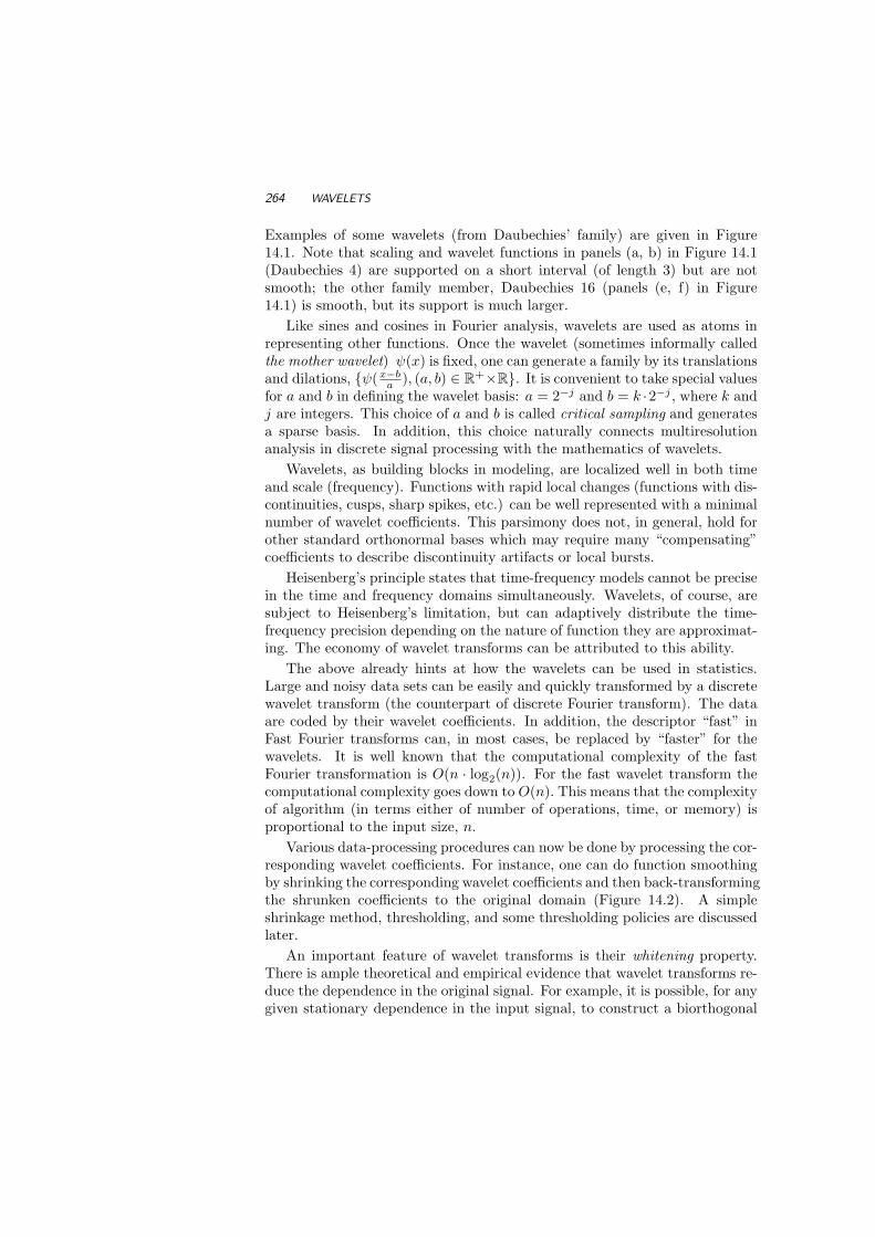
264 WAVELETS
Examples of some wavelets (from Daubechies’ family) are given in Figure14.1. Note that scaling and wavelet functions in panels (a, b) in Figure 14.1(Daubechies 4) are supported on a short interval (of length 3) but are notsmooth; the other family member, Daubechies 16 (panels (e, f) in Figure14.1) is smooth, but its support is much larger.
Like sines and cosines in Fourier analysis, wavelets are used as atoms inrepresenting other functions. Once the wavelet (sometimes informally calledthe mother wavelet) ψ(x) is fixed, one can generate a family by its translationsand dilations, ψ(x−b
a ), (a, b) ∈ R+×R. It is convenient to take special valuesfor a and b in defining the wavelet basis: a = 2−j and b = k ·2−j , where k andj are integers. This choice of a and b is called critical sampling and generatesa sparse basis. In addition, this choice naturally connects multiresolutionanalysis in discrete signal processing with the mathematics of wavelets.
Wavelets, as building blocks in modeling, are localized well in both timeand scale (frequency). Functions with rapid local changes (functions with dis-continuities, cusps, sharp spikes, etc.) can be well represented with a minimalnumber of wavelet coefficients. This parsimony does not, in general, hold forother standard orthonormal bases which may require many “compensating”coefficients to describe discontinuity artifacts or local bursts.
Heisenberg’s principle states that time-frequency models cannot be precisein the time and frequency domains simultaneously. Wavelets, of course, aresubject to Heisenberg’s limitation, but can adaptively distribute the time-frequency precision depending on the nature of function they are approximat-ing. The economy of wavelet transforms can be attributed to this ability.
The above already hints at how the wavelets can be used in statistics.Large and noisy data sets can be easily and quickly transformed by a discretewavelet transform (the counterpart of discrete Fourier transform). The dataare coded by their wavelet coefficients. In addition, the descriptor “fast” inFast Fourier transforms can, in most cases, be replaced by “faster” for thewavelets. It is well known that the computational complexity of the fastFourier transformation is O(n · log2(n)). For the fast wavelet transform thecomputational complexity goes down to O(n). This means that the complexityof algorithm (in terms either of number of operations, time, or memory) isproportional to the input size, n.
Various data-processing procedures can now be done by processing the cor-responding wavelet coefficients. For instance, one can do function smoothingby shrinking the corresponding wavelet coefficients and then back-transformingthe shrunken coefficients to the original domain (Figure 14.2). A simpleshrinkage method, thresholding, and some thresholding policies are discussedlater.
An important feature of wavelet transforms is their whitening property.There is ample theoretical and empirical evidence that wavelet transforms re-duce the dependence in the original signal. For example, it is possible, for anygiven stationary dependence in the input signal, to construct a biorthogonal
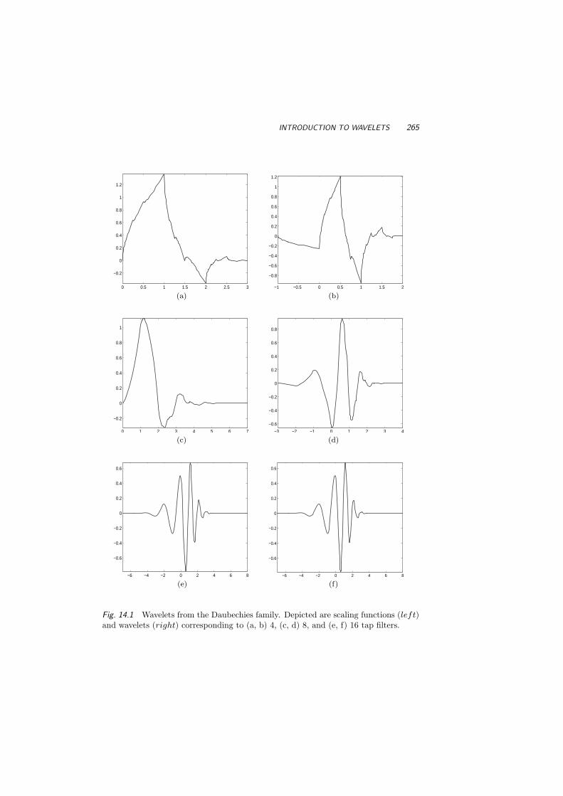
INTRODUCTION TO WAVELETS 265
0 0.5 1 1.5 2 2.5 3
−0.2
0
0.2
0.4
0.6
0.8
1
1.2
−1 −0.5 0 0.5 1 1.5 2
−0.8
−0.6
−0.4
−0.2
0
0.2
0.4
0.6
0.8
1
1.2
(a) (b)
0 1 2 3 4 5 6 7
−0.2
0
0.2
0.4
0.6
0.8
1
−3 −2 −1 0 1 2 3 4
−0.6
−0.4
−0.2
0
0.2
0.4
0.6
0.8
(c) (d)
−6 −4 −2 0 2 4 6 8
−0.6
−0.4
−0.2
0
0.2
0.4
0.6
−6 −4 −2 0 2 4 6 8
−0.6
−0.4
−0.2
0
0.2
0.4
0.6
(e) (f)
Fig. 14.1 Wavelets from the Daubechies family. Depicted are scaling functions (left)and wavelets (right) corresponding to (a, b) 4, (c, d) 8, and (e, f) 16 tap filters.

266 WAVELETS
Raw
Data
Wavelet
TransformShrinkage
Processed
Data
Inverse
Wavelet
Transform
Fig. 14.2 Wavelet-based data processing.
wavelet basis such that the corresponding in the transform are uncorrelated(a wavelet counterpart of the so called Karhunen-Loeve transform). For adiscussion and examples, see Walter and Shen (2001).
We conclude this incomplete inventory of wavelet transform features bypointing out their sensitivity to self-similarity in data. The scaling regularitiesare distinctive features of self-similar data. Such regularities are clearly visiblein the wavelet domain in the wavelet spectra, a wavelet counterpart of theFourier spectra. More arguments can be provided: computational speed ofthe wavelet transform, easy incorporation of prior information about somefeatures of the signal (smoothness, distribution of energy across scales), etc.
Basics on wavelets can be found in many texts, monographs, and papers atmany different levels of exposition. Student interested in the exposition thatis beyond this chapter coverage should consult monographs by Daubechies(1992), Ogden (1997), and Vidakovic (1999), and Walter and Shen (2001),among others.
14.2 HOW DO THE WAVELETS WORK?
14.2.1 The Haar Wavelet
To explain how wavelets work, we start with an example. We choose thesimplest and the oldest of all wavelets (we are tempted to say: grandmotherof all wavelets!), the Haar wavelet, ψ(x). It is a step function taking values1 and -1, on intervals [0, 1
2 ) and [ 12 , 1), respectively. The graphs of the Haarwavelet and some of its dilations/translations are given in Figure 14.4.
The Haar wavelet has been known for almost 100 years and is used invarious mathematical fields. Any continuous function can be approximateduniformly by Haar functions, even though the “decomposing atom” is discon-tinuous.
Dilations and translations of the function ψ,
ψjk(x) = const · ψ(2jx− k), j, k ∈ Z,

HOW DO THE WAVELETS WORK? 267
(a) (b) (c)
Fig. 14.3 (a) Jean Baptiste Joseph Fourier 1768–1830, Alfred Haar 1885–1933, and(c) Ingrid Daubechies, Professor at Princeton
x
0.0 0.2 0.4 0.6 0.8 1.0
-1.0
-0.5
0.0
0.5
1.0
(a) (b)
Fig. 14.4 (a) Haar wavelet ψ(x) = 1(0 ≤ x < 12)−1( 1
2< x ≤ 1); (b) Some dilations
and translations of Haar wavelet on [0,1].

268 WAVELETS
where Z = . . . ,−2,−1, 0, 1, 2, . . . is set of all integers, define an orthogonalbasis of L2(R) (the space of all square integrable functions). This means thatany function from L2(R) may be represented as a (possibly infinite) linearcombination of these basis functions.
The orthogonality of ψjk’s is easy to check. It is apparent that∫
ψjk · ψj′k′ = 0, (14.1)
whenever j = j′ and k = k′ are not satisfied simultaneously. If j 6= j′
(say j′ < j), then nonzero values of the wavelet ψj′k′ are contained in theset where the wavelet ψjk is constant. That makes integral in (14.1) equalto zero: If j = j′, but k 6= k′, then at least one factor in the productψj′k′ · ψjk is zero. Thus the functions ψij are mutually orthogonal. The con-stant that makes this orthogonal system orthonormal is 2j/2. The functionsψ10, ψ11, ψ20, ψ21, ψ22, ψ23 are depicted in Figure 14.4(b).
The family ψjk, j ∈ Z, k ∈ Z defines an orthonormal basis for L2. Alter-natively we will consider orthonormal bases of the form φL,k, ψjk, j ≥ L, k ∈Z, where φ is called the scaling function associated with the wavelet basisψjk, and φjk(x) = 2j/2φ(2jx − k). The set of functions φL,k, k ∈ Z spansthe same subspace as ψjk, j < L, k ∈ Z. For the Haar wavelet basis thescaling function is simple. It is an indicator of the interval [0,1), that is,
φ(x) = 1(0 ≤ x < 1).
The data analyst is mainly interested in wavelet representations of functionsgenerated by data sets. Discrete wavelet transforms map the data from thetime domain (the original or input data, signal vector) to the wavelet domain.The result is a vector of the same size. Wavelet transforms are linear and theycan be defined by matrices of dimension n×n when they are applied to inputsof size n. Depending on a boundary condition, such matrices can be eitherorthogonal or “close” to orthogonal. A wavelet matrix W is close to orthogonalwhen the orthogonality is violated by non-periodic handling of boundariesresulting in a small, but non-zero value of the norm ||WW ′ − I||, where Iis the identity matrix. When the matrix is orthogonal, the correspondingtransform can be thought is a rotation in Rn space where the data vectorsrepresent coordinates of points. For a fixed point, the coordinates in the new,rotated space comprise the discrete wavelet transformation of the originalcoordinates.
Example 14.1 Let y = (1, 0,−3, 2, 1, 0, 1, 2). The associated function f isgiven in Fig. 14.5. The values f(k) = yk, k = 0, 1, . . . , 7 are interpolatedby a piecewise constant function. The following matrix equation gives theconnection between y and the wavelet coefficients d, y = W ′d,

HOW DO THE WAVELETS WORK? 269
-3-2
-10
12
0 1 2 3 4 5 6 7 8
Fig. 14.5 A function interpolating y on [0,8).
10−321012
=
12√
21
2√
212 0 1√
20 0 0
12√
21
2√
212 0 − 1√
20 0 0
12√
21
2√
2− 1
2 0 0 1√2
0 01
2√
21
2√
2− 1
2 0 0 − 1√2
0 01
2√
2− 1
2√
20 1
2 0 0 1√2
01
2√
2− 1
2√
20 1
2 0 0 − 1√2
01
2√
2− 1
2√
20 − 1
2 0 0 0 1√2
12√
2− 1
2√
20 − 1
2 0 0 0 − 1√2
·
c00
d00
d10
d11
d20
d21
d22
d23
(14.2)
The solution is d = Wy,
c00
d00
d10
d11
d20
d21
d22
d23
=
√2
−√21−11√2
− 5√2
1√2
− 1√2
.

270 WAVELETS
Accordingly
f(x) =√
2φ0,0(x)−√
2ψ0,0(x) + ψ1,0(x)− ψ1,1(x) (14.3)
+1√2ψ2,0(x)− 5√
2ψ2,1(x) +
1√2ψ2,2(x)− 1√
2ψ2,3(x).
The solution is easy to verify. For example, when x ∈ [0, 1),
f(x) =√
2 · 12√
2−√
2 · 12√
2+ 1 · 1
2+
1√2· 1√
2= 1/2 + 1/2 = 1 (= y0).
The MATLAB m-file WavMat.m forms the wavelet matrix W , for a givenwavelet base and dimension which is a power of 2. For example, W = WavMat(h,n, k0, shift) will calculate n×n wavelet matrix, corresponding to the filterh (connections between wavelets and filtering will be discussed in the follow-ing section), and k0 and shift are given parameters. We will see that Haarwavelet corresponds to a filter h = √2/2,
√2/2. Here is the above example
in MATLAB:
>> W = WavMat([sqrt(2)/2 sqrt(2)/2],2^3,3,2);
>> W’
ans =
0.3536 0.3536 0.5000 0 0.7071 0 0 0
0.3536 0.3536 0.5000 0 -0.7071 0 0 0
0.3536 0.3536 -0.5000 0 0 0.7071 0 0
0.3536 0.3536 -0.5000 0 0 -0.7071 0 0
0.3536 -0.3536 0 0.5000 0 0 0.7071 0
0.3536 -0.3536 0 0.5000 0 0 -0.7071 0
0.3536 -0.3536 0 -0.5000 0 0 0 0.7071
0.3536 -0.3536 0 -0.5000 0 0 0 -0.7071
>> dat=[1 0 -3 2 1 0 1 2];
>> wt = W * dat’; wt’
ans =
1.4142 -1.4142 1.0000 -1.0000 0.7071 -3.5355 0.7071 -0.7071
>> data = W’ * wt; data’
ans =
1.0000 0.0000 -3.0000 2.0000 1.0000 0.0000 1.0000 2.0000
Performing wavelet transformations via the product of wavelet matrix Wand input vector y is conceptually straightforward, but of limited practicalvalue. Storing and manipulating wavelet matrices for inputs exceeding tensof thousands in length is not feasible.
14.2.2 Wavelets in the Language of Signal Processing
Fast discrete wavelet transforms become feasible by implementing the socalled cascade algorithm introduced by Mallat (1989). Let h(k), k ∈ Zand g(k), k ∈ Z be the quadrature mirror filters in the terminology of signal

HOW DO THE WAVELETS WORK? 271
processing. Two filters h and g form a quadrature mirror pair when:
g(n) = (−1)nh(1− n).
The filter h(k) is a low pass or smoothing filter while g(k) is the high pass ordetail filter. The following properties of h(n), g(n) can be derived by using socalled scaling relationship, Fourier transforms and orthogonality: Σkh(k) =√
2, Σkg(k) = 0, Σkh(k)2 = 1, and Σkh(k)k(k − 2m) = 1(m = 0).The most compact way to describe the cascade algorithm, as well to give
efficient recipe for determining discrete wavelet coefficients is by using operatorrepresentation of filters. For a sequence a = an the operators H and G aredefined by the following coordinate-wise relations:
(Ha)n = Σkh(k − 2n)ak
(Ga)n = Σkg(k − 2n)ak.
The operators H and G perform filtering and down-sampling (omitting everysecond entry in the output of filtering), and correspond to a single step inthe wavelet decomposition. The wavelet decomposition thus consists of sub-sequent application of operators H and G in the particular order on the inputdata.
Denote the original signal y by c(J). If the signal is of length n = 2J ,then c(J) can be understood as the vector of coefficients in a series f(x) =Σ2J−1
k=0 c(J)k φnk, for some scaling function φ. At each step of the wavelet trans-
form we move to a coarser approximation c(j−1) with c(j−1) = Hc(j) andd(j−1) = Gc(j). Here, d(j−1) represent the “details” lost by degrading c(j)
to c(j−1). The filters H and G are decimating, thus the length of c(j−1) ord(j−1) is half the length of c(j). The discrete wavelet transform of a sequencey = c(J) of length n = 2J can then be represented as another sequence oflength 2J (notice that the sequence c(j−1) has half the length of c(j)):
(c(0), d(0), d(1), . . . , d(J−2), d(J−1)). (14.4)
In fact, this decomposition may not be carried until the singletons c(0) andd(0) are obtained, but could be curtailed at (J − L)th step,
(c(L), d(L), d(L+1), . . . , d(J−2), d(J−1)), (14.5)
for any 0 ≤ L ≤ J − 1. The resulting vector is still a valid wavelet transform.See Exercise 14.4 for Haar wavelet transform “by hand.”
function dwtr = dwtr(data, L, filterh)
% function dwtr = dwt(data, L, filterh);
% Calculates the DWT of periodic data set
% with scaling filter filterh and L detail levels.
%
% Example of Use:
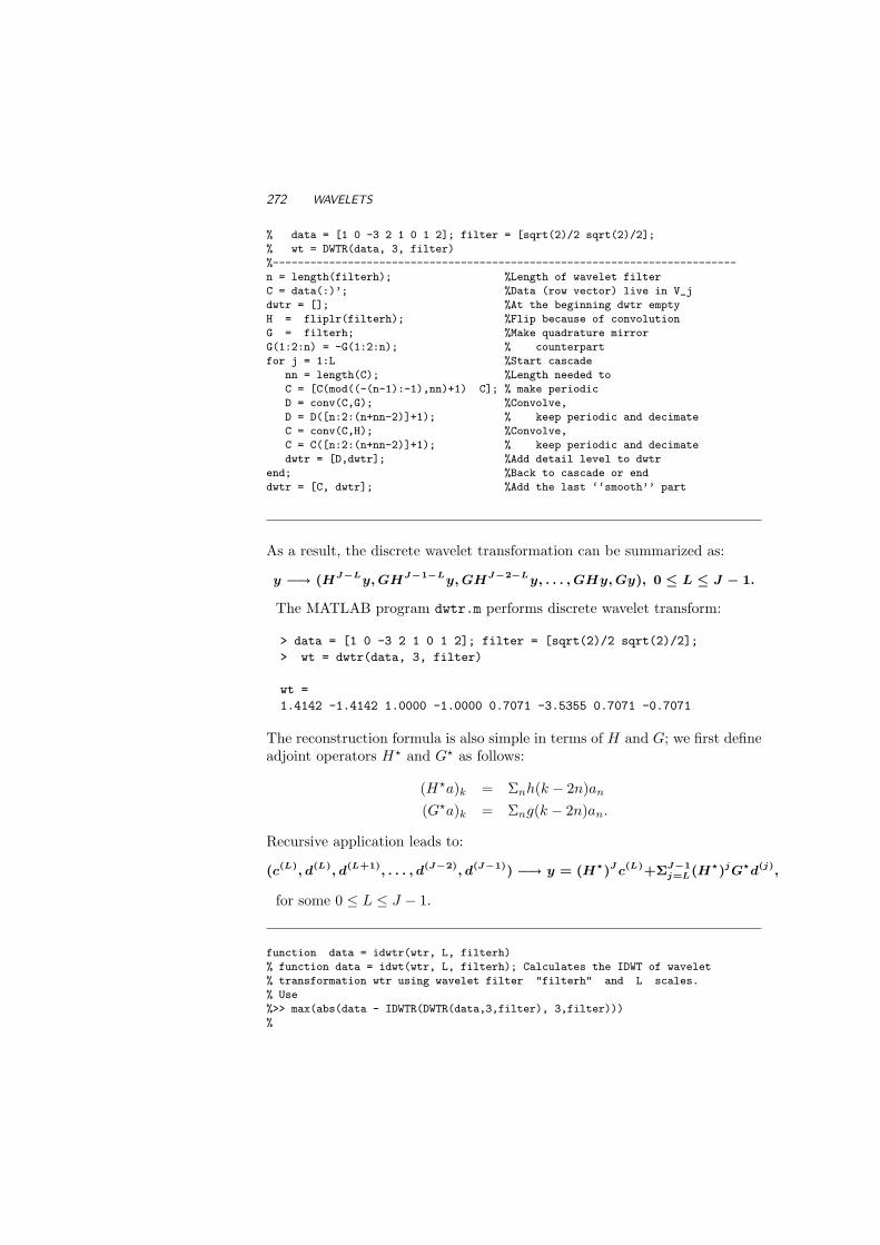
272 WAVELETS
% data = [1 0 -3 2 1 0 1 2]; filter = [sqrt(2)/2 sqrt(2)/2];
% wt = DWTR(data, 3, filter)
%--------------------------------------------------------------------------
n = length(filterh); %Length of wavelet filter
C = data(:)’; %Data (row vector) live in V_j
dwtr = []; %At the beginning dwtr empty
H = fliplr(filterh); %Flip because of convolution
G = filterh; %Make quadrature mirror
G(1:2:n) = -G(1:2:n); % counterpart
for j = 1:L %Start cascade
nn = length(C); %Length needed to
C = [C(mod((-(n-1):-1),nn)+1) C]; % make periodic
D = conv(C,G); %Convolve,
D = D([n:2:(n+nn-2)]+1); % keep periodic and decimate
C = conv(C,H); %Convolve,
C = C([n:2:(n+nn-2)]+1); % keep periodic and decimate
dwtr = [D,dwtr]; %Add detail level to dwtr
end; %Back to cascade or end
dwtr = [C, dwtr]; %Add the last ‘‘smooth’’ part
As a result, the discrete wavelet transformation can be summarized as:
y −→ (HJ−Ly, GHJ−1−Ly, GHJ−2−Ly, . . . , GHy, Gy), 0 ≤ L ≤ J − 1.
The MATLAB program dwtr.m performs discrete wavelet transform:
> data = [1 0 -3 2 1 0 1 2]; filter = [sqrt(2)/2 sqrt(2)/2];
> wt = dwtr(data, 3, filter)
wt =
1.4142 -1.4142 1.0000 -1.0000 0.7071 -3.5355 0.7071 -0.7071
The reconstruction formula is also simple in terms of H and G; we first defineadjoint operators H? and G? as follows:
(H?a)k = Σnh(k − 2n)an
(G?a)k = Σng(k − 2n)an.
Recursive application leads to:
(c(L), d(L), d(L+1), . . . , d(J−2), d(J−1)) −→ y = (H?)Jc(L)+ΣJ−1j=L(H?)jG?d(j),
for some 0 ≤ L ≤ J − 1.
function data = idwtr(wtr, L, filterh)
% function data = idwt(wtr, L, filterh); Calculates the IDWT of wavelet
% transformation wtr using wavelet filter "filterh" and L scales.
% Use
%>> max(abs(data - IDWTR(DWTR(data,3,filter), 3,filter)))
%

WAVELET SHRINKAGE 273
%ans = 4.4409e-016
nn = length(wtr); n = length(filterh); % Lengths
if nargin==2, L = round(log2(nn)); end; % Depth of transformation
H = filterh; % Wavelet H filter
G = fliplr(H); G(2:2:n) = -G(2:2:n); % Wavelet G filter
LL = nn/(2^L); % Number of scaling coeffs
C = wtr(1:LL); % Scaling coeffs
for j = 1:L % Cascade algorithm
w = mod(0:n/2-1,LL)+1; % Make periodic
D = wtr(LL+1:2*LL); % Wavelet coeffs
Cu(1:2:2*LL+n) = [C C(1,w)]; % Upsample & keep periodic
Du(1:2:2*LL+n) = [D D(1,w)]; % Upsample & keep periodic
C = conv(Cu,H) + conv(Du,G); % Convolve & add
C = C([n:n+2*LL-1]-1); % Periodic part
LL = 2*LL; % Double the size of level
end;
data = C; % The inverse DWT
Because wavelet filters uniquely correspond to selection of the waveletorthonormal basis, we give a table a few common (and short) filters commonlyused. See Table 14.19 for filters from the Daubechies, Coiflet and Symmletfamilies 1. See Exercise 14.5 for some common properties of wavelet filters.
The careful reader might have already noticed that when the length ofthe filter is larger than two, boundary problems occur (there are no bound-ary problems with the Haar wavelet). There are several ways to handle theboundaries, two main are: symmetric and periodic, that is, extending the orig-inal function or data set in a symmetric or periodic manner to accommodatefiltering that goes outside of domain of function/data.
14.3 WAVELET SHRINKAGE
Wavelet shrinkage provides a simple tool for nonparametric function estima-tion. It is an active research area where the methodology is based on optimalshrinkage estimators for the location parameters. Some references are Donohoand Johnstone (1994, 1995), Vidakovic (1999), Antoniadis, and Bigot and Sap-atinas (2001). In this section we focus on the simplest, yet most importantshrinkage strategy – wavelet thresholding.
In discrete wavelet transform the filter H is an “averaging” filter while itsmirror counterpart G produces details. The wavelet coefficients correspondto details. When detail coefficients are small in magnitude, they may be
1Filters are indexed by the number of taps and rounded at seven decimal places.

274 WAVELETS
Table 14.19 Some Common Wavelet Filters from the Daubechies, Coiflet and Symm-let Families.
Name h0 h1 h2 h3 h4 h5
Haar 1/√
2 1/√
2Daub 4 0.4829629 0.8365163 0.2241439 -0.1294095Daub 6 0.3326706 0.8068915 0.4598775 -0.1350110 -0.0854413 0.0352263Coif 6 0.0385808 -0.1269691 -0.0771616 0.6074916 0.7456876 0.2265843Daub 8 0.2303778 0.7148466 0.6308808 -0.0279838 -0.1870348 0.0308414Symm 8 -0.0757657 -0.0296355 0.4976187 0.8037388 0.2978578 -0.0992195Daub 10 0.1601024 0.6038293 0.7243085 0.1384281 -0.2422949 -0.0322449Symm 10 0.0273331 0.0295195 -0.0391342 0.1993975 0.7234077 0.6339789Daub 12 0.1115407 0.4946239 0.7511339 0.3152504 -0.2262647 -0.1297669Symm 12 0.0154041 0.0034907 -0.1179901 -0.0483117 0.4910559 0.7876411
Name h6 h7 h8 h9 h10 h11
Daub 8 0.0328830 -0.0105974Symm 8 -0.0126034 0.0322231Daub 10 0.0775715 -0.0062415 -0.0125808 0.0033357Symm 10 0.0166021 -0.1753281 -0.0211018 0.0195389Daub 12 0.0975016 0.0275229 -0.0315820 0.0005538 0.0047773 -0.0010773Symm 12 0.3379294 -0.0726375 -0.0210603 0.0447249 0.0017677 -0.0078007
omitted without substantially affecting the general picture. Thus the idea ofthresholding wavelet coefficients is a way of cleaning out unimportant detailsthat correspond to noise.
An important feature of wavelets is that they provide unconditional bases2
for functions that are more regular, smooth have fast decay of their waveletcoefficients. As a consequence, wavelet shrinkage acts as a smoothing opera-tor. The same can not be said about Fourier methods. Shrinkage of Fouriercoefficients in a Fourier expansion of a function affects the result globally dueto the non-local nature of sines and cosines. However, trigonometric basescan be localized by properly selected window functions, so that they providelocal, wavelet-like decompositions.
Why does wavelet thresholding work? Wavelet transforms disbalanceddata. Informally, the “energy” in data set (sum of squares of the data) ispreserved (equal to sum of squares of wavelet coefficients) but this energy ispacked in a few wavelet coefficients. This disbalancing property ensures thatthe function of interest can be well described by a relatively small number ofwavelet coefficients. The normal i.i.d. noise, on the other hand, is invariantwith respect to orthogonal transforms (e.g., wavelet transforms) and passes tothe wavelet domain structurally unaffected. Small wavelet coefficients likely
2Informally, a family ψi is an unconditional basis for a space of functions S if one candetermine if the function f = Σiaiψi belongs to S by inspecting only the magnitudes ofcoefficients, |ai|s.

WAVELET SHRINKAGE 275
correspond to a noise because the signal part gets transformed to a few big-magnitude coefficients.
The process of thresholding wavelet coefficients can be divided into twosteps. The first step is the policy choice, which is the choice of the thresh-old function T . Two standard choices are: hard and soft thresholding withcorresponding transformations given by:
Thard(d, λ) = d 1(|d| > λ),T soft(d, λ) = (d− sign(d)λ) 1(|d| > λ), (14.6)
where λ denotes the threshold, and d generically denotes a wavelet coefficient.Figure 14.6 shows graphs of (a) hard- and (b) soft-thresholding rules whenthe input is wavelet coefficient d.
d
hard
thre
shold
ing
-3 -2 -1 0 1 2 3
-3-2
-10
12
3
d
soft
thre
shold
ing
-3 -2 -1 0 1 2 3
-3-2
-10
12
3
(a) (b)
Fig. 14.6 (a) Hard and (b) soft thresholding with λ = 1.
Another class of useful functions are general shrinkage functions. A func-tion S from that class exhibits the following properties:
S(d) ≈ 0, for d small; S(d) ≈ d, for d large.
Many state-of-the-art shrinkage strategies are in fact of type S(d).The second step is the choice of a threshold if the shrinkage rule is thresh-
olding or appropriate parameters if the rule has S-functional form. In thefollowing subsection we briefly discuss some of the standard methods of se-lecting a threshold.

276 WAVELETS
14.3.1 Universal Threshold
In the early 1990s, Donoho and Johnstone proposed a threshold λ (Donohoand Johnstone, 1993; 1994) based on the result in theory of extrema of normalrandom variables.
Theorem 14.1 Let Z1, . . . , Zn be a sequence of i.i.d. standard normal ran-dom variables. Define
An = maxi=1,...,n
|Zi| ≤√
2 log n.
Then
πn = P (An) → 0, n →∞.
In addition, if
Bn(t) = maxi=1,...,n
|Zi| > t +√
2 log n,
then P (Bn(t)) < e−t22 .
Informally, the theorem states that the Zis are “almost bounded” by±√2 log n.Anything among the n values larger in magnitude than
√2 log n does not look
like the i.i.d. normal noise. This motivates the following threshold:
λU =√
2 log n σ, (14.7)
which Donoho and Johnstone call universal. This threshold is one of the firstproposed and provides an easy and automatic thresholding.
In the real-life problems the level of noise σ is not known, however waveletdomains are suitable for its assessment. Almost all methods for estimating thevariance of noise involve the wavelet coefficients at the scale of finest detail.The signal-to-noise ratio is smallest at this level for almost all reasonablybehaved signals, and the level coefficients correspond mainly to the noise.
Some standard estimators of σ are:
(i) σ =
√1
N/2− 1ΣN/2
k=1(dn−1,k − d)2, with d =1
N/2;Σdn−1,k (14.8)
or a more robust MAD estimator,
(ii) σ = 1/0.6745 mediank|dn−1,k −medianm(dn−1,m)|, (14.9)
where dn−1,k are coefficients in the level of finest detail. In some situations, forinstance when data sets are large or when σ is over-estimated, the universalthresholding oversmooths.

WAVELET SHRINKAGE 277
Example 14.2 The following MATLAB script demonstrates how the waveletssmooth the functions. A Doppler signal of size 1024 is generated and randomnormal noise of size σ = 0.1 is added. By using the Symmlet wavelet 8-tap fil-ter the noisy signal is transformed. After thresholding in the wavelet domainthe signal is back-transformed to the original domain.
% Demo of wavelet-based function estimation
clear all
close all
% (i) Make "Doppler" signal on [0,1]
t=linspace(0,1,1024);
sig = sqrt(t.*(1-t)).*sin((2*pi*1.05) ./(t+.05));
% and plot it
figure(1); plot(t, sig)
% (ii) Add noise of size 0.1. We are fixing
% the seed of random number generator for repeatability
% of example. We add the random noise to the signal
% and make a plot.
randn(’seed’,1)
sign = sig + 0.1 * randn(size(sig));
figure(2); plot(t, sign)
% (iii) Take the filter H, in this case this is SYMMLET 8
filt = [ -0.07576571478934 -0.02963552764595 ...
0.49761866763246 0.80373875180522 ...
0.29785779560554 -0.09921954357694 ...
-0.01260396726226 0.03222310060407];
% (iv) Transform the noisy signal in the wavelet domain.
% Choose L=8, eight detail levels in the decomposition.
sw = dwtr(sign, 8, filt);
% At this point you may view the sw. Is it disbalanced?
% Is it decorrelated?
%(v) Let’s now threshold the small coefficients.
% The universal threshold is determined as
% lambda = sqrt(2 * log(1024)) * 0.1 = 0.3723
%
% Here we assumed $sigma=0.1$ is known. In real life
% this is not the case and we estimate sigma.
% A robust estimator is ’MAD’ from the finest level of detail
% believed to be mostly transformed noise.
finest = sw(513:1024);
sigma_est = 1/0.6745 * median(abs( finest - median(finest)));
lambda = sqrt(2 * log(1024)) * sigma_est;
% hard threshold in the wavelet domain
swt=sw .* (abs(sw) > lambda );
figure(3); plot([1:1024], swt, ’-’)

278 WAVELETS
% (vi) Back-transform the thresholded object to the time
% domain. Of course, retain the same filter and value L.
sig_est = idwtr(swt, 8, filt);
figure(4); plot(t, sig_est, ’-’); hold on; plot(t, sig, ’:’);
0 0.2 0.4 0.6 0.8 1
−0.4
−0.3
−0.2
−0.1
0
0.1
0.2
0.3
0.4
0 0.2 0.4 0.6 0.8 1
−0.6
−0.4
−0.2
0
0.2
0.4
0.6
(a) (b)
200 400 600 800 1000
−4
−3
−2
−1
0
1
2
3
4
0 0.2 0.4 0.6 0.8 1−0.5
−0.4
−0.3
−0.2
−0.1
0
0.1
0.2
0.3
0.4
0.5
(c) (d)
Fig. 14.7 Demo output (a) Original doppler signal, (b) Noisy doppler, (c) Waveletcoefficients that “survived” thresholding, (d) Inverse-transformed thresholded coeffi-cients.
Example 14.3 A researcher was interested in predicting earthquakes by thelevel of water in nearby wells. She had a large (8192 = 213 measurements)data set of water levels taken every hour in a period of time of about one yearin a California well. Here is the description of the problem:
The ability of water wells to act as strain meters has been observed forcenturies. Lab studies indicate that a seismic slip occurs along a faultprior to rupture. Recent work has attempted to quantify this response,in an effort to use water wells as sensitive indicators of volumetric strain.If this is possible, water wells could aid in earthquake prediction bysensing precursory earthquake strain.
We obtained water level records from a well in southern California,collected over a year time span. Several moderate size earthquakes(magnitude 4.0 - 6.0) occurred in close proximity to the well duringthis time interval. There is a a significant amount of noise in the wa-ter level record which must first be filtered out. Environmental factors

WAVELET SHRINKAGE 279
such as earth tides and atmospheric pressure create noise with frequen-cies ranging from seasonal to semidiurnal. The amount of rainfall alsoaffects the water level, as do surface loading, pumping, recharge (suchas an increase in water level due to irrigation), and sonic booms, toname a few. Once the noise is subtracted from the signal, the recordcan be analyzed for changes in water level, either an increase or a de-crease depending upon whether the aquifer is experiencing a tensile orcompressional volume strain, just prior to an earthquake.
This data set is given in earthquake.dat. A plot of the raw data forhourly measurements over one year (8192 = 213 observations) is given inFigure 14.8(a). The detail showing the oscillation at the earthquake time ispresented in Figure 14.8(b).
Julian Day
Leve
l
400 500 600
-53.5
-53.4
-53.3
-53.2
-53.1
-53.0
••••••••
•••••••••••••••••••••
•
•
•
•
•
•••
•
•••••••••••••••
•••••••••••••••••
•
Julian Day
Leve
l
416.0 416.5 417.0 417.5 418.0 418.5
-53.5
-53.4
-53.3
-53.2
-53.1
-53.0
(a) (b)
Juilan Day
Leve
l
400 500 600
-53.
5-5
3.4
-53.
3-5
3.2
-53.
1
Julian Day
Leve
l
400 500 600
-53.
6-5
3.5
-53.
4-5
3.3
-53.
2-5
3.1
(c) (d)
Fig. 14.8 Panel (a) shows n = 8192 hourly measurements of the water level for a wellin an earthquake zone. Notice the wide range of water levels at the time of an earth-quake around t = 417. Panel (b) focusses on the data around the earthquake time.Panel (c) shows the result of LOESS, and (d) gives a wavelet based reconstruction.

280 WAVELETS
Application of LOESS smoother captured trend but the oscillation artifactis smoothed out as evident from Figure 14.8(c). After applying the Daubechies8 wavelet transform and universal thresholding we got a fairly smooth baselinefunction with preserved jump at the earthquake time. The processed data arepresented in Figure 14.8(d). This feature of wavelet methods demonstrateddata adaptivity and locality.
How this can be explained? The wavelet coefficients corresponding to theearthquake feature (big oscillation) are large in magnitude and are located atall even the finest detail level. These few coefficients “survived” the thresh-olding, and the oscillation feature shows in the inverse transformation. SeeExercise 14.6 for the suggested follow-up.
-H
G -
HcHrA HcGrA
?
G H
?
?
G H
?
Fig. 14.9 One step in wavelet transformation of 2-D data exemplified on celebratedLenna image.

EXERCISES 281
Example 14.4 The most important application of 2-D wavelets is in imageprocessing. Any gray-scale image can be represented by a matrix A in whichthe entries aij correspond to color intensities of the pixel at location (i, j). Weassume as standardly done that A is a square matrix of dimension 2n× 2n, ninteger.
The process of wavelet decomposition proceeds as follows. On the rows ofthe matrix A the filters H and G are applied. Two resulting matrices HrAand GrA are obtained, both of dimension 2n × 2n−1 (Subscript r suggestthat the filters are applied on rows of the matrix A, 2n−1 is obtained in thedimension of HrA and GrA because wavelet filtering decimate). Now, thefilters H and G are applied on the columns of HrA and GrA and matricesHcHrA,GcHrA,HcGrA and GcGrA of dimension 2n−1 × 2n−1 are obtained.The matrix HcHrA is the average, while the matrices GcHrA,HcGrA andGcGrA are details (see Figure 14.9).3
The process could be continued in the same fashion with the smoothedmatrix HcHrA as an input, and can be carried out until a single number isobtained as an overall “smooth” or can be stopped at any step. Notice thatin decomposition exemplified in Figure 14.9, the matrix is decomposed to onesmooth and three detail submatrices.
A powerful generalization of wavelet bases is the concept of wavelet pack-ets. Wavelet packets result from applications of operators H and G, discussedon p. 271, in any order. This corresponds to an overcomplete system of func-tions from which the best basis for a particular data set can be selected.
14.4 EXERCISES
14.1. Show that the matrix W ′ in (14.2) is orthogonal.
14.2. In (14.1) we argued that ψjk and ψj′k′ are orthogonal functions wheneverj = j′ and k = k′ is not satisfied simultaneously. Argue that φjk andψj′k′ are orthogonal whenever j′ ≥ j. Find an example in which φjk andψj′k′ are not orthogonal if j′ < j.
14.3. In Example 14.1 it was verified that in (14.3) f(x) = 1 whenever x ∈[0, 1). Show that f(x) = 0 whenever x ∈ [1, 2).
14.4. Verify that (√
2,−√2, 1,−1, 1√2,− 5√
2, 1√
2,− 1√
2) is a Haar wavelet trans-
form of data set y = (1, 0,−3, 2, 1, 0, 1, 2) by using operators H and Gfrom (14.4).
3This image of Lenna (Sjooblom) Soderberg, a Playboy centerfold from 1972, has becomeone of the most widely used standard test images in signal processing.

282 WAVELETS
Hint. For the Haar wavelet, low- and high-pass filters are h = (1/√
2 1/√
2)and g = (1/
√2 − 1/
√2), so
Hy = H((1, 0,−3, 2, 1, 0, 1, 2))
= (1 · 1/√
2 + 0 · 1/√
2, − 3 · 1/√
2 + 2 · 1/√
2,
1 · 1/√
2 + 0 · 1/√
2, 1 · 1/√
2 + 2 · 1/√
2)
=(
1√2,− 1√
2,
1√2,
3√2
), and
Gy = G((1, 0,−3, 2, 1, 0, 1, 2)) =(
1√2,− 5√
2,
1√2,− 1√
2
).
Repeat the G operator on Hy and H(Hy). The final filtering is H(H(Hy)).Organize result as
(H(H(Hy)), G(H(Hy)), G(Hy), Gy) .
14.5. Demonstrate that all filters in Table 14.19 satisfy the following proper-ties (up to rounding error):
Σihi =√
2, Σih2i = 1, and Σihihi+2 = 0.
14.6. Refer to Example 14.3 in which wavelet-based smoother exhibited no-table difference from the standard smoother LOESS. Read the dataearthquake.dat into MATLAB, select the wavelet filter, and apply thewavelet transform to the data.
(a) Estimate the size of the noise by estimating σ using MAD from page276 and find the universal threshold λU .
(b) Show that finest level of detail contains coefficients exceeding theuniversal threshold.
(c) Threshold the wavelet coefficients using hard thresholding rule withλU that you have obtained in (b), and apply inverse wavelet transform.Comment. How do you explain oscillations at boundaries?

REFERENCES 283
REFERENCES
Antoniadis, A., Bigot, J., and Sapatinas, T. (2001), “Wavelet Estimators inNonparametric Regression: A Comparative Simulation Study,” Journalof Statistical Software, 6, 1-83.
Daubechies, I. (1992), Ten Lectures on Wavelets. Philadelphia: S.I.A.M.Donoho, D., and Johnstone, I. (1994), “Ideal Spatial Adaptation by Wavelet
Shrinkage,” Biometrika, 81, 425-455.Donoho, D., and Johnstone, I. (1995), Adapting to Unknown Smoothness via
Wavelet Shrinkage,” Journal of the American Statistical Association, 90,1200-1224.
Donoho, D., Johnstone, I., Kerkyacharian, G., and Pickard, D. (1996), “Den-sity Estimation by Wavelet Thresholding,” Annals of Statistics, 24, 508-539.
Mallat, S. (1989), “A Theory for Multiresolution Signal Decomposition: TheWavelet Representation,” IEEE Transactions on Pattern Analysis andMachine Intelligence, 11, 674-693.
Ogden, T. (1997), Essential Wavelets for Statistical Applications and DataAnalysis. Boston: Birkhauser.
Vidakovic, B. (1999), Statistical Modeling by Wavelets, New York: Wiley.Walter, G.G., and Shen X. (2001), Wavelets and Others Orthogonal Systems,
2nd ed. Boca Raton, FL: Chapman & Hall/CRC.


15Bootstrap
Confine! I’ll confine myself no finer than I am:these clothes are good enough to drink in; and so be these boots too:an they be not, let them hang themselves in their own straps.
William Shakespeare (Twelfth Night, Act 1, Scene III)
15.1 BOOTSTRAP SAMPLING
Bootstrap resampling is one of several controversial techniques in statisticsand according to some, the most controversial. By resampling, we mean totake a random sample from the sample, as if your sampled data X1, . . . , Xn
represented a finite population of size n. This new sample (typically of thesame size n) is taken by “sampling with replacement”, so some of the n itemsfrom the original sample can appear more than once. This new collectionis called a bootstrap sample, and can be used to assess statistical propertiessuch as an estimator’s variability and bias, predictive performance of a rule,significance of a test, and so forth, when the exact analytic methods areimpossible or intractable.
By simulating directly from the data, the bootstrap avoids making un-necessary assumptions about parameters and models – we are figurativelypulling ourselves up by our bootstraps rather than relying on the outside helpof parametric assumptions. In that sense, the bootstrap is a nonparametricprocedure. In fact, this resampling technique includes both parametric and
285

286 BOOTSTRAP
(a) (b)
Fig. 15.1 (a) Bradley Efron, Stanford University; (b) Prasanta Chandra Mahalanobis(1893–1972)
nonparametric forms, but it is essentially empirical.The term bootstrap was coined by Bradley Efron (Figure 15.1(a)) at his
1977 Stanford University Reitz Lecture to describe a resampling method thatcan help us to understand characteristics of an estimator (e.g., uncertainty,bias) without the aid of additional probability modeling. The bootstrap de-scribed by Efron (1979) is not the first resampling method to help out thisway (e.g., permutation methods of Fisher (1935) and Pitman (1937), spatialsampling methods of Mahalanobis (1946), or jack-knife methods of Quenouille(1949)), but it’s the most popular resampling tool used in statistics today.
So what good is a bootstrap sample? For any direct inference on theunderlying distribution, it is obviously inferior to the original sample. If weestimate a parameter θ = θ(F ) from a distribution F , we obviously preferto use θn = θ(Fn). What the bootstrap sample can tell us, is how θn mightchange from sample to sample. While we can only compute θn once (becausewe have just the one sample of n), we can resample (and form a bootstrapsample) an infinite amount of times, in theory. So a meta-estimator built froma bootstrap sample (say θ) tells us not about θ, but about θn. If we generaterepeated bootstrap samples θ1, . . . , θB , we can form an indirect picture of howθn is distributed, and from this we generate confidence statements for θ. B isnot really limited – it’s as large as you want as long as you have the patiencefor generating repeated bootstrap samples.
For example, x ± zα/2σx constitutes an exact (1-α)100% confidence in-terval for µ if we know X1, . . . , Xn ∼ N (µ, σ2) and σx = σ/
√n. We are
essentially finding the appropriate quantiles from the sampling distributionof point estimate x. Unlike this simple example, characteristics of the sam-ple estimator often are much more difficult to ascertain, and even an intervalbased on a normal approximation seems out of reach or provide poor coverageprobability. This is where resampling comes in most useful.

NONPARAMETRIC BOOTSTRAP 287
Fig. 15.2 Baron Von Munchausen: the first bootstrapper.
The idea of bootstrapping was met with initial trepidation. After all, itmight seem to be promising something for nothing. The stories of Baron VonMunchausen (Raspe, 1785), based mostly on folk tales, include astoundingfeats such as riding cannonballs, travelling to the Moon and being swallowedby a whale before escaping unharmed. In one adventure, the baron escapesfrom a swamp by pulling himself up by his own hair. In later versions he wasusing his own bootstraps to pull himself out of the sea, which gave rise to theterm bootstrapping.
15.2 NONPARAMETRIC BOOTSTRAP
The percentile bootstrap procedure provides a 1-α nonparametric confidenceinterval for θ directly. We examine the EDF from the bootstrap sample forθ1 − θn, . . . , θB − θn. If θn is a good estimate of θ, then we know θ − θn
is a good estimate of θn − θ. We don’t know the distribution of θn − θbecause we don’t know θ, so we cannot use the quantiles from θn − θ toform a confidence interval. But we do know the distribution of θ − θn, andthe quantiles serve the same purpose. Order the outcomes of the bootstrapsample (θ1 − θn, . . . , θB − θn). Choose the α/2 and 1− α/2 sample quantiles
288 BOOTSTRAP
from the bootstrap sample: [θ(1− α/2)− θn, θ(α/2)− θn]. Then
P(θ(1− α/2)− θn < θ − θn < θ(α/2)− θn
)
= P(θ(1− α/2) < θ < θ(α/2)
)≈ 1− α.
The quantiles of the bootstrap samples form an approximate confidence in-terval for θ that is computationally simple to construct.
Parametric Case. If the actual data are assumed to be generated from adistribution F (x; θ) (with unknown θ), we can improve over the nonparametricbootstrap. Instead of resampling from the data, we can generate a moreefficient bootstrap sample by simulating data from F (x; θn).
Example 15.1 Hubble Telescope and Hubble Correlation. The Hub-ble constant (H) is one of the most important numbers in cosmology becauseit is instrumental in estimating the size and age of the universe. This long-sought number indicates the rate at which the universe is expanding, from theprimordial “Big Bang.” The Hubble constant can be used to determine the in-trinsic brightness and masses of stars in nearby galaxies, examine those sameproperties in more distant galaxies and galaxy clusters, deduce the amount ofdark matter present in the universe, obtain the scale size of faraway galaxyclusters, and serve as a test for theoretical cosmological models.
In 1929, Edwin Hubble (Figure 15.3(a)) investigated the relationship be-tween the distance of a galaxy from the earth and the velocity with whichit appears to be receding. Galaxies appear to be moving away from us nomatter which direction we look. This is thought to be the result of the BigBang. Hubble hoped to provide some knowledge about how the universe wasformed and what might happen in the future. The data collected includedistances (megaparsecs1) to n = 24 galaxies and their recessional velocities(km/sec). The scatter plot of the pairs is given in Figure 15.3(b). Hubble’slaw claims that Recessional Velocity is directly proportional to the Distanceand the coefficient of proportionality is Hubble’s constant, H. By workingbackward in time, the galaxies appear to meet in the same place. Thus 1/Hcan be used to estimate the time since the Big Bang – a measure of the age ofthe universe. Thus, because of this simple linear model, it is important to es-timate correlation between distances and velocities and see if the no-interceptlinear regression model is appropriate.
11 parsec = 3.26 light years.
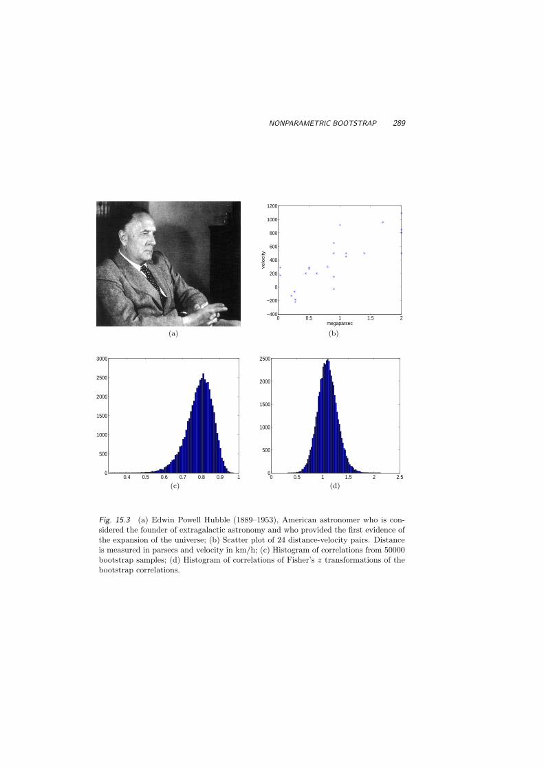
NONPARAMETRIC BOOTSTRAP 289
0 0.5 1 1.5 2−400
−200
0
200
400
600
800
1000
1200
megaparsec
velo
city
(a) (b)
0.4 0.5 0.6 0.7 0.8 0.9 10
500
1000
1500
2000
2500
3000
0 0.5 1 1.5 2 2.50
500
1000
1500
2000
2500
(c) (d)
Fig. 15.3 (a) Edwin Powell Hubble (1889–1953), American astronomer who is con-sidered the founder of extragalactic astronomy and who provided the first evidence ofthe expansion of the universe; (b) Scatter plot of 24 distance-velocity pairs. Distanceis measured in parsecs and velocity in km/h; (c) Histogram of correlations from 50000bootstrap samples; (d) Histogram of correlations of Fisher’s z transformations of thebootstrap correlations.
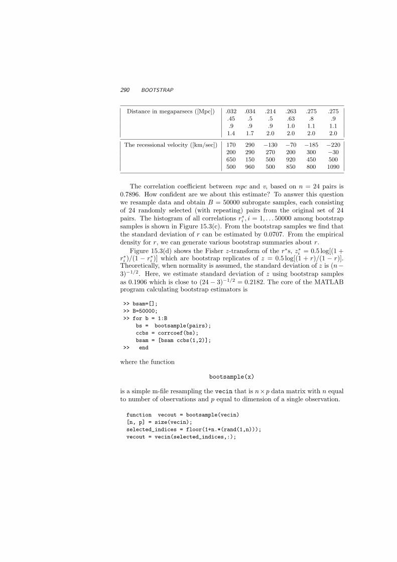
290 BOOTSTRAP
Distance in megaparsecs ([Mpc]) .032 .034 .214 .263 .275 .275.45 .5 .5 .63 .8 .9.9 .9 .9 1.0 1.1 1.11.4 1.7 2.0 2.0 2.0 2.0
The recessional velocity ([km/sec]) 170 290 −130 −70 −185 −220200 290 270 200 300 −30650 150 500 920 450 500500 960 500 850 800 1090
The correlation coefficient between mpc and v, based on n = 24 pairs is0.7896. How confident are we about this estimate? To answer this questionwe resample data and obtain B = 50000 subrogate samples, each consistingof 24 randomly selected (with repeating) pairs from the original set of 24pairs. The histogram of all correlations r∗i , i = 1, . . . 50000 among bootstrapsamples is shown in Figure 15.3(c). From the bootstrap samples we find thatthe standard deviation of r can be estimated by 0.0707. From the empiricaldensity for r, we can generate various bootstrap summaries about r.
Figure 15.3(d) shows the Fisher z-transform of the r∗s, z∗i = 0.5 log[(1 +r∗i )/(1 − r∗i )] which are bootstrap replicates of z = 0.5 log[(1 + r)/(1 − r)].Theoretically, when normality is assumed, the standard deviation of z is (n−3)−1/2. Here, we estimate standard deviation of z using bootstrap samplesas 0.1906 which is close to (24 − 3)−1/2 = 0.2182. The core of the MATLABprogram calculating bootstrap estimators is
>> bsam=[];
>> B=50000;
>> for b = 1:B
bs = bootsample(pairs);
ccbs = corrcoef(bs);
bsam = [bsam ccbs(1,2)];
>> end
where the function
bootsample(x)
is a simple m-file resampling the vecin that is n×p data matrix with n equalto number of observations and p equal to dimension of a single observation.
function vecout = bootsample(vecin)
[n, p] = size(vecin);
selected_indices = floor(1+n.*(rand(1,n)));
vecout = vecin(selected_indices,:);

NONPARAMETRIC BOOTSTRAP 291
Example 15.2 Trimmed Mean. For robust estimation of the populationmean, outliers can be trimmed off the sample, ensuring the estimator willbe less influenced by tails of the distribution. If we trim off almost all of thedata, we will end up using the sample median. Suppose we trim off 50% of thedata by excluding the smallest and largest 25% of the sample. Obviously, thestandard error of this estimator is not easily tractable, so no exact confidenceinterval can be constructed. This is where the bootstrap technique can helpout. In this example, we will focus on constructing a two-sided 95% confidenceinterval for µ, where
µ =
∫ x3/4
x1/4tdF (t)
F (x3/4)− F (x1/4)= 2
∫ x3/4
x1/4
tdF (t)
is an alternative measure of central tendency, the same as the populationmean if the distribution is symmetric.
If we compute the trimmed mean from the sample as µn, it is easy togenerate bootstrap samples and do the same. In this case, limiting B to 1000or 2000 will make computing easier, because each repeated sample must beranked and trimmed before µ can be computed. Let µ(.025) and µ(.975) bethe lower and upper quantiles from the bootstrap sample µ1, . . . , µB .
The MATLAB m-file trimmean(x,P) trims P% (so 0 < P < 100) of thedata, or P/2% of the biggest and smallest observations. The MATLAB m-file
ciboot(x,’trimmean’,5,.90,1000,10)
acquires 1000 bootstrap samples from x, performs the trimmean function (itsadditional argument, P=10, is left on the end) and a 90% (2-sided) confidenceinterval is generated. The middle value is the point estimate. Below, thevector x represents a skewed sample of test scores, and a 90% confidenceinterval for the trimmed mean is (57.6171, 89.9474). The third argument inthe ciboot function can take on integer values between one and six, and thisinput dictates the type of bootstrap to construct. The input options are
1. Normal approximation (std is bootstrap).
2. Simple bootstrap principle (bad, don’t use).
3. Studentized, std is computed via jackknife.
4. Studentized, std is 30 samples’ bootstrap.
5. Efron’s pctl method.
6. Efron’s pctl method with bias correction(default)

292 BOOTSTRAP
>> x = [11,13,14,32,55,58,61,67,69,73,73,89,90,93,94,94,95,96,99,99];
>> m = trimmean(x,10)
m =
71.7895
>> m2 = mean(x)
m2 =
68.7500
>> ciboot(x,’trimmean’,5,.90,1000,10)
ans =
57.6171 71.7895 82.9474
Estimating Standard Error. The most common application of a simplebootstrap is to estimate the standard error of the estimator θn. The algorithmis similar to the general nonparametric bootstrap:
• Generate B bootstrap samples of size n.
• Evaluate the bootstrap estimators θ1, . . . , θB .
• Estimate standard error of θn as
σθn =
√√√√ΣBi=1
(θi − θ∗
)2
B − 1,
where θ∗ = B−1Σθi.
15.3 BIAS CORRECTION FOR NONPARAMETRIC INTERVALS
The percentile method described in the last section is simple, easy to use,and has good large sample properties. However, the coverage probability isnot accurate for many small sample problems. The Acceleration and Bias-Correction (or BCa) method improves on the percentile method by adjustingthe percentiles (e.g., θ(1−α/2, θ(α/2)) chosen from the bootstrap sample. Adetailed discussion is provided in Efron and Tibshirani (1993).
The BCa interval is determined by the proportion of the bootstrap esti-mates θ less than θn, i.e., p0 = B−1ΣI(θi < θn) define the bias factor as
z0 = Φ−1(p0)
express this bias, where Φ is the standard normal CDF, so that values of z0

BIAS CORRECTION FOR NONPARAMETRIC INTERVALS 293
away from zero indicate a problem. Let
a0 =ΣB
i=1
(θ∗ − θi
)3
6(ΣB
i=1(θ∗ − θi)2)3/2
be the acceleration factor, where θ∗ is the average of the bootstrap estimatesθ1, . . . , θB . It gets this name because it measures the rate of change in σθn
asa function of θ.
Finally, the 100(1− α)% BCa interval is computed as
[ θ(q1), θ(q2) ],
where
q1 = Φ(
z0 +z0 + zα/2
1− a0(z0 + zα/2)
),
q2 = Φ(
z0 +z0 + z1−α/2
1− a0(z0 + z1−α/2)
).
Note that if z0 = 0 (no measured bias) and a0 = 0, then (15.1) is thesame as the percentile bootstrap interval. In the MATLAB m-file ciboot,the BCa is an option (6) for the nonparametric interval. For the trimmedmean example, the bias corrected interval is shifted upward:
>> ciboot(x,’trimmean’,6,.90,1000,10)
ans =
60.0412 71.7895 84.4211
Example 15.3 Recall the data from Crowder et al. (1991) which was dis-cussed in Example 10.2. The data contain strength measurements (in codedunits) for 48 pieces of weathered cord. Seven of the pieces of cord were dam-aged and yielded strength measurements that are considered right censored.The following MATLAB code uses a bias-corrected bootstrap to calculate a95% confidence interval for the probability that the strength measure is equalto or less than 50, that is, F (50).
>> data = [36.3, 41.7, 43.9, 49.9, 50.1, 50.8, 51.9, 52.1, 52.3, 52.3,...
52.4, 52.6, 52.7, 53.1, 53.6, 53.6, 53.9, 53.9, 54.1, 54.6,...
54.8, 54.8, 55.1, 55.4, 55.9, 56.0, 56.1, 56.5, 56.9, 57.1,...
57.1, 57.3, 57.7, 57.8, 58.1, 58.9, 59.0, 59.1, 59.6, 60.4,...
60.7, 26.8, 29.6, 33.4, 35.0, 40.0, 41.9, 42.5];
>> censor=[ones(1,41), zeros(1,7)];
>> [kmest, sortdat, sortcen] = KMcdfSM(data’, censor’, 0);
>> prob = kmest( sum( 50.0 >=data), 1)
prob =

294 BOOTSTRAP
0.0949
>> function fkmt = kme_at_50(dt)
% this function performs Kaplan-Meier
% estimation with given parameter
% and produces estimated F(50.0)
[kmest sortdat] = KMcdfSM(dt(:,1), dt(:,2), 0);
fkmt = kmest(sum(50.0 >= sortdat), 1);
Using kme at 50.m and ciboot functions we obtain a confidence interval forF (50) based on 1000 bootstrap replicates:
>> ciboot([data’ censor’], ’kme_at_50’, 5, .95, 1000)
ans =
0.0227 0.0949 0.1918
>> % a 95% CI for F(50) is (0.0227, 0.1918)
>> function fkmt = kme_all_x(dt)
% this function performs Kaplan-Meier estimation with given parameter
% and gives estimated F() for all data points
[kmest sortdat] = KMcdfSM(dt(:,1), dt(:,2), 0);
data = [36.3, 41.7, //...deleted...//, 41.9, 42.5];
temp_val = [];
%calculate each CDF F() value for all data points
for i=1:length(data)
if sum(data(i) >= sortdat) > 0
temp_val = [temp_val kmest(sum(data(i) >= sortdat), 1)];
else % when there is no observation, CDF is simply 0
temp_val = [temp_val 0];
end
end
fkmt = temp_val;
The MATLAB functions ciboot and kme all x are used to produce Figure15.4:
>> ci = ciboot([data’ censor’], ’kme_all_x’, 5, .95, 1000);
>> figure;
>> plot(data’, ci(:,2)’, ’.’);
>> hold on;
>> plot(data’, ci(:,1)’, ’+’);
>> plot(data’, ci(:,3)’, ’*’);

THE JACKKNIFE 295
25 30 35 40 45 50 55 60 650
0.1
0.2
0.3
0.4
0.5
0.6
0.7
0.8
0.9
1
Fig. 15.4 95% confidence band the CDF of Crowder’s data using 1000 bootstrapsamples. Lower boundary of the confidence band is plotted with marker ’+’, while theupper boundary is plotted with marker ’*’.
15.4 THE JACKKNIFE
The jackknife procedure, introduced by Quenouille (1949), is a resamplingmethod for estimating bias and variance in θn. It predates the bootstrap andactually serves as a special case. The resample is based on the “leave oneout” method, which was computationally easier when computing resourceswere limited.
The ith jackknife sample is (x1, . . . , xi−1, xi+1, ..., xn). Let θ(i) be the esti-mator of θ based only on the ith jackknife sample. The jackknife estimate ofthe bias is defined as
bJ = (n− 1)(θn − θ∗
),
where θ∗ = n−1Σθ(i). The jackknife estimator for the variance of θn is
σJ2 =
n− 1n
Σni=1
(θ(i) − θ∗
)2
.
The jackknife serves as a poor man’s version of the bootstrap. That is, itestimates bias and variance the same, but with a limited resampling mecha-nism. In MATLAB, the m-file
jackknife(x,function,p1,...)
produces the jackknife estimate for the input function. The function jackrsp(x,k)produces a matrix of jackknife samples (taking k elements out, with defaultof k = 1).
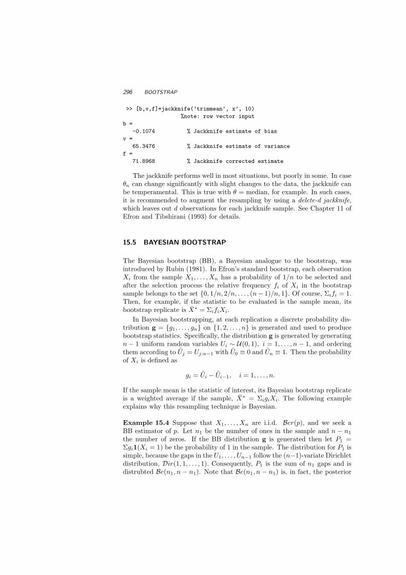
296 BOOTSTRAP
>> [b,v,f]=jackknife(’trimmean’, x’, 10)
%note: row vector input
b =
-0.1074 % Jackknife estimate of bias
v =
65.3476 % Jackknife estimate of variance
f =
71.8968 % Jackknife corrected estimate
The jackknife performs well in most situations, but poorly in some. In caseθn can change significantly with slight changes to the data, the jackknife canbe temperamental. This is true with θ = median, for example. In such cases,it is recommended to augment the resampling by using a delete-d jackknife,which leaves out d observations for each jackknife sample. See Chapter 11 ofEfron and Tibshirani (1993) for details.
15.5 BAYESIAN BOOTSTRAP
The Bayesian bootstrap (BB), a Bayesian analogue to the bootstrap, wasintroduced by Rubin (1981). In Efron’s standard bootstrap, each observationXi from the sample X1, . . . , Xn has a probability of 1/n to be selected andafter the selection process the relative frequency fi of Xi in the bootstrapsample belongs to the set 0, 1/n, 2/n, . . . , (n− 1)/n, 1. Of course, Σifi = 1.Then, for example, if the statistic to be evaluated is the sample mean, itsbootstrap replicate is X∗ = ΣifiXi.
In Bayesian bootstrapping, at each replication a discrete probability dis-tribution g = g1, . . . , gn on 1, 2, . . . , n is generated and used to producebootstrap statistics. Specifically, the distribution g is generated by generatingn − 1 uniform random variables Ui ∼ U(0, 1), i = 1, . . . , n − 1, and orderingthem according to Uj = Uj:n−1 with U0 ≡ 0 and Un ≡ 1. Then the probabilityof Xi is defined as
gi = Ui − Ui−1, i = 1, . . . , n.
If the sample mean is the statistic of interest, its Bayesian bootstrap replicateis a weighted average if the sample, X∗ = ΣigiXi. The following exampleexplains why this resampling technique is Bayesian.
Example 15.4 Suppose that X1, . . . , Xn are i.i.d. Ber(p), and we seek aBB estimator of p. Let n1 be the number of ones in the sample and n − n1
the number of zeros. If the BB distribution g is generated then let P1 =Σgi1(Xi = 1) be the probability of 1 in the sample. The distribution for P1 issimple, because the gaps in the U1, . . . , Un−1 follow the (n−1)-variate Dirichletdistribution, Dir(1, 1, . . . , 1). Consequently, P1 is the sum of n1 gaps and isdistrubted Be(n1, n − n1). Note that Be(n1, n− n1) is, in fact, the posterior

BAYESIAN BOOTSTRAP 297
for P1 if the prior is ∝ [P1(1− P1)]−1. That is, for x ∈ 0, 1,
P (X = x|P1) = P x1 (1− P1)1−x, P1 ∝ [P1(1− P1)]−1,
then the posterior is
[P1|X1, . . . , Xn] ∼ Be(n1, n− n1).
For general case when Xi take d ≤ n different values the Bayesian interpreta-tion is still valid; see Rubin’s (1981) article.
Example 15.5 We revisit Hubble’s data and give a BB estimate of variabilityof observed coefficient of correlation r. For each BB distribution g calculate
r∗ =Σn
i=1giXiYi − (Σni−1giXi)(Σn
i−1giXi)[Σn
i=1giX2i − (Σn
i=1giXi)2]1/2 [Σni=1giY 2
i − (Σni=1giYi)2]1/2
,
where (Xi, Yi), i = 1, . . . 24 are observed pairs of distances and velocities. TheMATLAB program below performs the BB resampling.
>> x = [0.032 0.034 0.214 0.263 0.275 0.275 0.45 0.5 0.5 0.63
0.8 0.9 0.9 0.9 0.9 1.0 1.1 1.1 1.4 1.7 2.0 2.0 2.0 2.0 ]; %Mpc
>> y = [170 290 -130 -70 -185 -220 200 290 270 200 300 -30 ...
650 150 500 920 450 500 500 960 500 850 800 1090]; %velocity
>> n=24; corr(x’, y’);
>> B=50000; %number of BB replicates
>> bbcorr = []; %store BB correlation replicates
>> for i = 1:B
sampl = (rand(1,n-1));
osamp = sort(sampl);
all = [0 osamp 1];
gis = diff(all, 1);
% gis is BB distribution, corrbb is correlation
% with gis as weights
ssx = sum(gis .* x); ssy = sum( gis .* y);
ssx2 = sum(gis .* x.^2); ssy2 = sum(gis .* y.^2);
ssxy = sum(gis .* x .* y);
corrbb = (ssxy - ssx * ssy)/...
sqrt((ssx2 - ssx^2)*(ssy2 - ssy^2)); %correlation replicate
bbcorr=[bbcorr corrbb]; %add replicate to the storage sequence
>> end
>> figure(1)
>> hist(bbcorr,80)
>> std(bbcorr)
>> zs = 1/2 * log((1+bbcorr)./(1-bbcorr)); %Fisher’s z
>> figure(2)
>> hist(zs,80)
>> std(zs)

298 BOOTSTRAP
0.4 0.5 0.6 0.7 0.8 0.9 10
500
1000
1500
2000
2500
0 0.5 1 1.5 20
500
1000
1500
2000
2500
(a) (b)
Fig. 15.5 The histogram of 50,000 BB resamples for the correlation between thedistance and velocity in the Hubble data; (b) Fisher z-transform of the BB correlations.
The histograms of correlation bootstrap replicates and their z-transformsin Figure 15.5 (a-b) look similar to the those in Figure 15.3 (c-d). Numerically,B = 50, 000 replicates gave standard deviation of observed r as 0.0635 andstandard deviation of z = 1/2 log((1 + r)/(1 − r)) as 0.1704 slightly smallerthan theoretical 24− 3−1/2 = 0.2182.
15.6 PERMUTATION TESTS
Suppose that in a statistical experiment the sample or samples are takenand a statistic S is constructed for testing a particular hypothesis H0. Thevalues of S that seem extreme from the viewpoint of H0 are critical for thishypothesis. The decision if the observed value of statistics S is extreme ismade by looking at the distribution of S when H0 is true. But what if suchdistribution is unknown or too complex to find? What if the distribution forS is known only under stringent assumptions that we are not willing to make?
Resampling methods consisting of permuting the original data can be usedto approximate the null distribution of S. Given the sample, one forms thepermutations that are consistent with experimental design and H0, and thencalculates the value of S. The values of S are used to estimate its density(often as a histogram) and using this empirical density we find an approximatep-value, often called a permutation p-value.
What permutations are consistent with H0? Suppose that in a two-sample

PERMUTATION TESTS 299
problem we want to compare the means of two populations based on two in-dependent samples X1, . . . , Xm and Y1, . . . , Yn. The null hypothesis H0 isµX = µY . The permutations consistent with H0 would be all permutationsof a combined (concatenated) sample X1, . . . , Xm, Y1, . . . , Yn. Or suppose wea repeated measures design in which observations are triplets correspondingto three treatments, i.e., (X11, X12, X13), . . . , (Xn1, Xn2, Xn3), and that H0
states that the three treatment means are the same, µ1 = µ2 = µ3. Then per-mutations consistent with this experimental design are random permutationsamong the triplets (Xi1, Xi2, Xi3), i = 1, . . . , n and a possible permutationmight be
(X13, X11, X12), (X21, X23, X22), (X32, X33, X31), . . . , (Xn2, Xn1, Xn3).
Thus, depending on the design and H0, consistent permutations can be quitedifferent.
Example 15.6 Byzantine Coins. To illustrate the spirit of permutationtests we use data from a paper by Hendy and Charles (1970) (see also Handet al, 1994) that represent the silver content (%Ag) of a number of Byzantinecoins discovered in Cyprus. The coins (Figure 15.6) are from the first andfourth coinage in the reign of King Manuel I, Comnenus (1143–1180).
1st coinage 5.9 6.8 6.4 7.0 6.6 7.7 7.2 6.9 6.24th coinage 5.3 5.6 5.5 5.1 6.2 5.8 5.8
The question of interest is whether or not there is statistical evidence tosuggest that the silver content of the coins was significantly different in thelater coinage.
Fig. 15.6 A coin of Manuel I Comnenus (1143–1180).
Of course, the two-sample t-test or one of its nonparametric counterpartsis possible to apply here, but we will use the permutation test for purposes ofillustration. The following MATLAB commands perform the test:

300 BOOTSTRAP
>> coins=[5.9 6.8 6.4 7.0 6.6 7.7 7.2 6.9 6.2 ...
>> 5.3 5.6 5.5 5.1 6.2 5.8 5.8];
>> coins1=coins(1:9); coins2=coins(10:16);
>> S = (mean(coins1)-mean(coins2))/sqrt(var(coins1)+var(coins2))
>> Sps =[]; asl=0; %Sps is permutation S,
>> %asl is achieved significance level
>> N=10000;
>> for i = 1:N
coinsp=coins(randperm(16));
coinsp1=coinsp(1:9); coinsp2=coinsp(10:16);
Sp = (mean(coinsp1)-mean(coinsp2))/ ...
sqrt(var(coinsp1)+var(coinsp2));
Sps = [Sps Sp ];
asl = asl + (abs(Sp) > S );
end
>> asl = asl/N
The value for S is 1.7301, and the permutation p-value or the achievedsignificance level is asl = 0.0004. Panel (a) in Figure 15.7 shows the permu-tation null distribution of statistics S and the observed value of S is indicatedby the dotted vertical line. Note that there is nothing special about selecting
S =X1 − X2√
s21/n1 + s2
2/n2
,
and that any other statistics that sensibly measures deviation from H0 :µ1 = µ2 could be used. For example, one could use S = median(X1)/s1 −median(X2)/s2, or simply S = X1 − X2.
To demonstrate how the choice what to permute depends on statistical de-sign, we consider again the two sample problem but with paired observations.In this case, the permutations are done within the pairs, independently frompair to pair.
Example 15.7 Left-handed Grippers. Measurements of the left- andright-hand gripping strengths of 10 left-handed writers are recorded.
Person 1 2 3 4 5 6 7 8 9 10
Left hand (X) 140 90 125 130 95 121 85 97 131 110
Right hand (Y) 138 87 110 132 96 120 86 90 129 100
Do the data provide strong evidence that people who write with their lefthand have greater gripping strength in the left hand than they do in the righthand?

PERMUTATION TESTS 301
In the MATLAB solution provided below, dataL and dataR are pairedmeasurements and pdataL and pdataR are random permutations, either 1, 2or 2, 1 of the 10 original pairs. The statistics S is the difference of thesample means. The permutation null distribution is shown as non-normalizedhistogram in Figure 15.7(b). The position of S with respect to the histogramis marked by dotted line.
>> dataL =[ 140 , 90 , 125 , 130 , 95 , 121 , 85 , 97 , 131 , 110 ];
>> dataR =[ 138 , 87 , 110 , 132 , 96 , 120 , 86 , 90 , 129 , 100 ];
>> S=mean(dataL - dataR)
>> data =[dataL; dataR];
>> means=[]; asl =0; N=10000;
>> for i = 1:N
pdata=[];
for j=1:10
pairs = data(randperm(2),j);
pdata = [pdata pairs];
end
pdataL = pdata(1,:);
pdataR = pdata(2,:);
pmean=mean(pdataL - pdataR);
means= [means pmean];
asl = asl + (abs(pmean) > S);
end
−2 −1.5 −1 −0.5 0 0.5 1 1.5 20
100
200
300
400
500
600
700
800
900
−5 0 50
200
400
600
800
(a) (b)
Fig. 15.7 Panels (a) and (b) show permutation null distribution of statistics S andthe observed value of S (marked by dotted line) for the cases of (a) Bizantine coins,and (b) Left-handed grippers.
302 BOOTSTRAP
15.7 MORE ON THE BOOTSTRAP
There are several excellent resources for learning more about bootstrap tech-niques, and there are many different kinds of bootstraps that work on variousproblems. Besides Efron and Tibshirani (1993), books by Chernick (1999) andDavison and Hinkley (1997) provide excellent overviews with numerous help-ful examples. In the case of dependent data various bootstrapping strategiesare proposed such as block bootstrap, stationary bootstrap, wavelet-basedbootstrap (wavestrap), and so on. A monograph by Good (2000) gives acomprehensive coverage of permutation tests.
Bootstrapping is not infallible. Data sets that might lead to poor perfor-mance include those with missing values and excessive censoring. Choice ofstatistics is also critical; see Exercise 15.6. If there are few observations in thetail of the distribution, bootstrap statistics based on the EDF perform poorlybecause they are deduced using only a few of those extreme observations.
15.8 EXERCISES
15.1. Generate a sample of 20 from the gamma distribution with λ = 0.1 andr=3. Compute a 90% confidence interval for the mean using (a) thestandard normal approximation, (b) the percentile method and (c) thebias-corrected method. Repeat this 1000 times and report the actualcoverage probability of the three intervals you constructed.
15.2. For the case of estimating the sample mean with X, derive the expectedvalue of the jackknife estimate of bias and variance.
15.3. Refer to insect waiting times for the female Western White Clematis inTable 10.15. Use the percentile method to find a 90% confidence intervalfor F (30), the probability that the waiting time is less than or equal to30 minutes.
15.4. In a data set of size n generated from a continuous F , how many distinctbootstrap samples are possible?
15.5. Refer to the dominance-submissiveness data in Exercise 7.3. Construct a95% confidence interval for the correlation using the percentile bootstrapand the jackknife. Compare your results with the normal approximationdescribed in Section 2 of Chapter 7.
15.6. Suppose we have three observations from U(0, θ). If we are interestedin estimating θ, the MLE for it is θ = X3:3, the largest observation. Ifwe obtain a bootstrap sampling procedure to estimate the variance ofthe MLE, what is the distribution of the bootstrap estimator for θ?

EXERCISES 303
15.7. Seven patients each underwent three different methods of kidney dialy-sis. The following values were obtained for weight change in kilogramsbetween dialysis sessions:
Patient Treatment 1 Treatment 2 Treatment 3
1 2.90 2.97 2.672 2.56 2.45 2.623 2.88 2.76 1.844 2.73 2.20 2.335 2.50 2.16 1.276 3.18 2.89 2.397 2.83 2.87 2.39
Test the null hypothesis that there is no difference in mean weight changeamong treatments. Use properly designed permutation test.
15.8. In a controlled clinical trial Physician’s Health Study I which began in1982 and ended in 1987, more that 22,000 physicians participated. Theparticipants were randomly assigned to two groups: (i) Aspirin and (ii)Placebo, where the aspirin group have been taking 325 mg aspirin everysecond day. At the end of trial, the number of participants who sufferedfrom Myocardial Infarction was assessed. The counts are given in thefollowing table:
MyoInf No MyoInf Total
Aspirin 104 10933 11037Placebo 189 10845 11034
The popular measure in assessing results in clinical trials is Risk Ra-tio (RR) which is the ratio of proportions of cases (risks) in the twogroups/treatments. From the table,
RR = Ra/Rp =104/11037189/11034
= 0.55.
Interpretation of RR is that the risk of Myocardial Infarction for thePlacebo group is approximately 1/0.55 = 1.82 times higher than thatfor the Aspirin group. With MATLAB, construct a bootstrap estimatefor the variability of RR. Hint:
aspi = [zeros(10933,1); ones(104,1)];
plac = [zeros(10845,1); ones(189,1)];
RR = (sum(aspi)/length(aspi))/(sum(plac)/length(plac));

304 BOOTSTRAP
BRR = [ ]; B=10000;
for b = 1:B
baspi = bootsample(aspi);
bplac = bootsample(plac);
BRR = [BRR (sum(baspi)/length(baspi))/(sum(bplac)/length(bplac))];
end
(ii) Find the variability of the difference of the risks Ra − Rp, and oflogarithm of the odds ratio, log(Ra/(1−Ra))− log(Rp/(1−Rp)).
(iii) Using the Bayesian bootstrap, estimate the variability of RR, Ra−Rp, and log(Ra/(1−Ra))− log(Rp/(1−Rp)).
15.9. Let fi and gi be frequency/probability of the observation Xi in an ordi-nary/Bayesian bootstrap resample from X1, . . . , Xn. Prove that Efi =Egi = 1/n, i.e., the expected probability distribution is discrete uniform,Varfi = (n + 1)/n, Vargi = (n − 1)/n2, and for i 6= j, Corr(fi, fj) =Corr(gi, gj) = −1/(n− 1).
REFERENCES
Davison, A. C., and Hinkley, D. V. (1997), Bootstrap Methods and TheirApplications, Boston: Cambridge University Press.
Chernick, M. R., (1999), Bootstrap Methods – A Practitioner’s Guide, NewYork: Wiley.
Efron, B., and Tibshirani, R. J. (1993), An Introduction to the Bootstrap,Boca Raton, FL: CRC Press.
Efron, B. (1979), “Bootstrap Methods: Another Look at the Jackknife,” An-nals of Statistics, 7, 1-26
Fisher, R.A. (1935), The Design of Experiments, New York: Hafner.Good, P. I. (2000), Permutation Tests: A Practical Guide to Resampling
Methods for Testing Hypotheses, 2nd ed., New York: Springer Verlag.Hand, D.J., Daly, F., Lunn, A.D., McConway, K.J., and Ostrowski, E. (1994),
A Handbook of Small Datasets, New York: Chapman & Hall.Hendy, M. F., and Charles, J. A. (1970), “The Production Techniques, Sil-
ver Content, and Circulation History of the Twelfth-Century ByzantineTrachy,” Archaeometry, 12, 13-21.
Mahalanobis, P. C. (1946), “On Large-Scale Sample Surveys,” PhilosophicalTransactions of the Royal Society of London, Ser. B, 231, 329–451.
Pitman, E. J. G., (1937), “Significance Tests Which May Be Applied to Sam-ples from Any Population,” Royal Statistical Society Supplement, 4, 119–130 and 225–232 (parts I and II).

REFERENCES 305
Quenouille, M. H. (1949), “Approximate Tests of Correlation in Time Series,”Journal of the Royal Statistical Society, Ser. B, 11, 18–84.
Raspe, R. E. (1785). The Travels and Surprising Adventures of Baron Mun-chausen, London: Trubner, 1859 [1st Ed. 1785].
Rubin, D. (1981), “The Bayesian Bootstrap,” Annals of Statistics, 9, 130-134.


16EM Algorithm
Insanity is doing the same thing over and over again and expectingdifferent results.
Albert Einstein
The Expectation-Maximization (EM) algorithm is broadly applicable sta-tistical technique for maximizing complex likelihoods while handling problemswith incomplete data. Within each iteration of the algorithm, two steps areperformed: (i) the E-Step consisting of projecting an appropriate functionalcontaining the augmented data on the space of the original, incomplete data,and (ii) the M -Step consisting of maximizing the functional.
The name EM algorithm was coined by Dempster, Laird, and Rubin (1979)in their fundamental paper, referred to here as the DLR paper. But as isusually the case, if one comes to a smart idea, one may be sure that other smartguys in the history had already thought about it. Long before, McKendrick(1926) and Healy and Westmacott (1956) proposed iterative methods thatare examples of the EM algorithm. In fact, before the DLR paper appearedin 1997, dozens of papers proposing various iterative solvers were essentiallyapplying the EM Algorithm in some form.
However, the DLR paper was the first to formally recognize these separatealgorithms as having the same fundamental underpinnings, so perhaps their1977 paper prevented further reinventions of the same basic math tool. Whilethe algorithm is not guaranteed to converge in every type of problem (asmistakenly claimed by DLR), Wu (1983) showed convergence is guaranteedif the densities making up the full data belong to the exponential family.
307

308 EM ALGORITHM
This does not prevent the EM method from being helpful in nonparametricproblems; Tsai and Crowley (1985) first applied it to a general nonparametricsetting and numerous applications have appeared since.
16.0.1 Definition
Let Y be a random vector corresponding to the observed data y and havinga postulated PDF f(y, ψ), where ψ = (ψ1, . . . , ψd) is a vector of unknownparameters. Let x be a vector of augmented (so called complete) data, andlet z be the missing data that completes x, so that x = [y, z].
Denote by gc(x, ψ) the PDF of the random vector corresponding to thecomplete data set x. The log-likelihood for ψ, if x were fully observed, wouldbe
log Lc(ψ) = log gc(x, ψ).
The incomplete data vector y comes from the “incomplete” sample spaceY. There is an one-to-one correspondence between the complete sample spaceX and the incomplete sample space Y. Thus, for x ∈ X , one can uniquelyfind the “incomplete” y = y(x) ∈ Y. Also, the incomplete pdf can be foundby properly integrating out the complete pdf,
g(y, ψ) =∫
X (y)
gc(x, ψ)dx,
where X (y) is the subset of X constrained by the relation y = y(x).Let ψ(0) be some initial value for ψ. At the k-th step the EM algorithm
one performs the following two steps:
E-Step. Calculate
Q(ψ, ψ(k)) = Eψ(k)log Lc(ψ)|y.
M-Step. Choose any value ψ(k+1) that maximizes Q(ψ,ψ(k)), that is,
(∀ψ)Q(ψ(k+1), ψ(k)) ≥ Q(ψ, ψ(k)).
The E and M steps are alternated until the difference
L(ψ(k+1))− L(ψ(k))
becomes small in absolute value.Next we illustrate the EM algorithm with a famous example first consid-
ered by Fisher and Balmukand (1928). It is also discussed in Rao (1973), andlater by Mclachlan and Krishnan (1997) and Slatkin and Excoffier (1996).

FISHER’S EXAMPLE 309
16.1 FISHER’S EXAMPLE
The following genetics example was recognized by as an application of theEM algorithm by Dempster et al. (1979). The description provided hereessentially follows a lecture by Terry Speed of UC at Berkeley. In basic geneticsterminology, suppose there are two linked bi-allelic loci, A and B, with allelesA and a, and B and b, respectively, where A is dominant over a and B isdominant over b. A double heterozygote AaBb will produce gametes of fourtypes: AB, Ab, aB and ab. As the loci are linked, the types AB and ab willappear with a frequency different from that of Ab and aB, say 1 − r and r,respectively, in males, and 1− r′ and r′ respectively in females.
Here we suppose that the parental origin of these heterozygotes is fromthe mating AABB × aabb, so that r and r′ are the male and female recom-bination rates between the two loci. The problem is to estimate r and r′, ifpossible, from the offspring of selfed double heterozygotes. Because gametesAB, Ab,aB and ab are produced in proportions (1−r)/2, r/2, r/2 and (1−r)/2,respectively, by the male parent, and (1− r′)/2, r′/2, r′/2 and (1− r′)/2, re-spectively, by the female parent, zygotes with genotypes AABB,AaBB, . . .etc, are produced with frequencies (1− r)(1− r′)/4, (1− r)r′/4, etc.
The problem here is this: although there are 16 distinct offspring geno-types, taking parental origin into account, the dominance relations imply thatwe only observe 4 distinct phenotypes, which we denote by A∗B∗, A∗b∗, a∗B∗
and a∗b∗. Here A∗(respectively B∗) denotes the dominant, while a∗ (respec-tively b∗) denotes the recessive phenotype determined by the alleles at A(respectively B).
Thus individuals with genotypes AABB,AaBB,AABb or AaBb, (whichaccount for 9/16 of the gametic combinations) exhibit the phenotype A∗B∗,i.e. the dominant alternative in both characters, while those with genotypesAAbb or Aabb (3/16) exhibit the phenotype A∗b∗, those with genotypes aaBBand aaBb (3/16) exhibit the phenotype a∗B∗, and finally the double recessiveaabb (1/16) exhibits the phenotype a∗b∗. It is a slightly surprising fact thatthe probabilities of the four phenotypic classes are definable in terms of theparameter ψ = (1 − r)(1 − r′), as follows: a∗b∗ has probability ψ/4 (easy tosee), a∗B∗ and A∗b∗ both have probabilities (1−ψ)/4, while A∗B∗ has rest ofthe probability, which is (2+ψ)/4. Now suppose we have a random sample of noffspring from the selfing of our double heterozygote. The 4 phenotypic classeswill be represented roughly in proportion to their theoretical probabilities,their joint distribution being multinomial
Mn
(n;
2 + ψ
4,1− ψ
4,1− ψ
4,ψ
4
). (16.1)
Note that here neither r nor r′ will be separately estimable from these data,but only the product (1 − r)(1 − r′). Because we know that r ≤ 1/2 andr′ ≤ 1/2, it follows that ψ ≥ 1/4.

310 EM ALGORITHM
How do we estimate ψ? Fisher and Balmukand listed a variety of methodsthat were in the literature at the time, and compare them with maximumlikelihood, which is the method of choice in problems like this. We describe avariant on their approach to illustrate the EM algorithm.
Let y = (125, 18, 20, 34) be a realization of vector y = (y1, y2, y3, y4) be-lieved to be coming from the multinomial distribution given in (16.1). Theprobability mass function, given the data, is
g(y, ψ) =n!
y1!y2!y3!y4!(1/2 + ψ/4)y1 (1/4− ψ/4)y2+y3 (ψ/4)y4 .
The log likelihood, after omitting an additive term not containing ψ is
log L(ψ) = y1 log(2 + ψ) + (y2 + y3) log(1− ψ) + y4 log(ψ).
By differentiating with respect to ψ one gets
∂ log L(ψ)/∂ψ =y1
2 + ψ− y2 + y3
1− ψ+
y4
ψ.
The equation ∂ log L(ψ)/∂ψ = 0 can be solved and solution is ψ = (15 +√53809)/394 ≈ 0.626821.Now assume that instead of original value y1 the counts y11 and y12,
such that y11 + y12 = y1, could be observed, and that their probabilitiesare 1/2 and ψ/4, respectively. The complete data can be defined as x =(y11, y12, y2, y3, y4). The probability mass function of incomplete data y isg(y, ψ) = Σgc(x, ψ), where
gc(x, ψ) = c(x)(1/2)y11(ψ/4)y12(1/4− ψ/4)y2+y3(ψ/4)y4 ,
c(x) is free of ψ, and the summation is taken over all values of x for whichy11 + y12 = y1.
The complete log likelihood is
log Lc(ψ) = (y12 + y4) log(ψ) + (y2 + y3) log(1− ψ). (16.2)
Our goal is to find the conditional expectation of log Lc(ψ) given y, using thestarting point for ψ(0),
Q(ψ, ψ(0)) = Eψ(0)log Lc(ψ)|y.
As log Lc is linear function in y11 and y12, the E-Step is done by simply byreplacing y11 and y12 by their conditional expectations, given y. If Y11 is therandom variable corresponding to y11, it is easy to see that
Y11 ∼ Bin
(y1,
1/21/2 + ψ(0)/4
)

MIXTURES 311
so that the conditional expectation of Y11 given y1 is
Eψ(0)(Y11|y1) =y12
12 + ψ(0)
4
= y(0)11 .
Of course, y(0)12 = y1 − y
(0)11 . This completes the E-Step part.
In the M-Step one chooses ψ(1) so that Q(ψ,ψ(0)) is maximized. Afterreplacing y11 and y12 by their conditional expectations y
(0)11 and y
(0)12 in the
Q-function, the maximum is obtained at
ψ(1) =y(0)12 + y4
y(0)12 + y2 + y3 + y4
=y(0)12 + y4
n− y(0)11
.
The EM-Algorithm is composed of alternating these two steps. At theiteration k we have
ψ(k+1) =y(k)12 + y4
n− y(k)11
,
where y(k)11 = 1
2y1/(1/2 + ψ(k)/4) and y(k)12 = y1 − y
(k)11 . To see how the EM
algorithm computes the MLE for this problem, see the MATLAB functionemexample.m.
16.2 MIXTURES
Recall from Chapter 2 that mixtures are compound distributions of the formF (x) =
∫F (x|t)dG(t). The CDF G(t) serves as a mixing distribution on ker-
nel distribution F (x|t). Recognizing and estimating mixtures of distributionsis an important task in data analysis. Pattern recognition, data mining andother modern statistical tasks often call for mixture estimation.
For example, suppose an industrial process that produces machine partswith lifetime distribution F1, but a small proportion of the parts (say, ω) aredefective and have CDF F2 À F1. If we cannot sort out the good ones fromthe defective ones, the lifetime of a randomly chosen part is
F (x) = (1− ω)F1(x) + ωF2(x).
This is a simple two-point mixture where the mixing distribution has twodiscrete points of positive mass. With (finite) discrete mixtures like this, theprobability points of G serve as weights for the kernel distribution. In thenonparametric likelihood, we see immediately how difficult it is to solve forthe MLE in the presence of the weight ω, especially if ω is unknown.
Suppose we want to estimate the weights of a fixed number k of fully known

312 EM ALGORITHM
distributions. We illustrate EM approach which introduces unobserved indi-cators with the goal of simplifying the likelihood. The weights are estimatedby maximum likelihood. Assume that a sample X1, X2, . . . , Xn comes fromthe mixture
f(x, ω) = Σkj=1ωjfj(x),
where f1, . . . , fk are continuous and the weights 0 ≤ ωj ≤ 1 are unknown andconstitute (k − 1)-dimensional vector ω = (ω1, . . . , ωk−1) and ωk = 1 − ω1 −· · · − ωk−1. The class-densities fj(x) are fully specified.
Even in this simplest case when f1, . . . , fk are given and the only param-eters are the weights ω, the log-likelihood assumes a complicated form,
Σni=1 log f(xi, ω) = Σn
i=1 log(Σk
j=1ωjfj(xi))
.
The derivatives with respect to ωj lead to the system of equations, not solvablein a closed form.
Here is a situation where the EM Algorithm can be applied with a littlecreative foresight. Augment the data x = (x1, . . . , xn) by an unobservablematrix z = (zij , i = 1, . . . , n; j = 1, . . . , k). The values zij are indicators,defined as
zij =
1, xi from fj
0, otherwise
The unobservable matrix z (our “missing value”) tells us (in an oracular fash-ion) where the ith observation xi comes from. Note that each row of z containsa single 1 and k−1 0’s. With augmented data, x = (y, z) the (complete) like-lihood takes quite a simple form,
n∏
i=1
k∏
j=1
(ωjfj(xi))zij .
The complete log-likelihood is simply
log Lc(ω) = Σni=1Σ
kj=1zij log ωj + C,
where C = ΣiΣjzij log fj(xi) is free of ω. This is easily solved.Assume that mth iteration of the weight estimate ω(m) is already obtained.
The mth E-Step is
Eω(m)(zij |x) = Pω(m)(zij = 1|x) = z(k)ij ,
where z(m)ij is the posterior probability of ith observation coming from the jth

MIXTURES 313
mixture-component, fj , in the iterative step m.
z(m)ij =
ω(m)j fj(xi)
f(xi, ω(m)).
Because log Lc(ω) is linear in zij , Q(ω, ω(m)) is simply Σni=1Σ
kj=1z
(m)ij log ωj +
C. The subsequent M-Step is simple: Q(ω, ω(m)) is maximized by
ω(m+1)j =
Σni=1z
(m)ij
n.
The MATLAB script (mixture cla.m) illustrates the algorithm above. Asample of size 150 is generated from the mixture f(x) = 0.5N (−5, 22) +0.3N (0, 0.52)+0.2N (2, 1). The mixing weights are estimated by the EM algo-rithm. M = 20 iterations of EM algorithm yielded ω = (0.4977, 0.2732, 0.2290).Figure 16.1 gives histogram of data, theoretical mixture and EM estimate.
−10 −5 0 50
0.05
0.1
0.15
0.2
0.25
Fig. 16.1 Observations from the 0.5N (−5, 22) + 0.3N (0, 0.52) + 0.2N (2, 1) mixture(histogram), the mixture (dotted line) and EM estimated mixture (solid line).
Example 16.1 As an example of a specific mixture of distributions we con-sider application of EM algorithm in the so called Zero Inflated Poisson (ZIP)model. In ZIP models the observations come from two populations, one inwhich all values are identically equal to 0 and the other Poisson P(λ). The“zero” population is selected with probability ξ, and the Poisson population
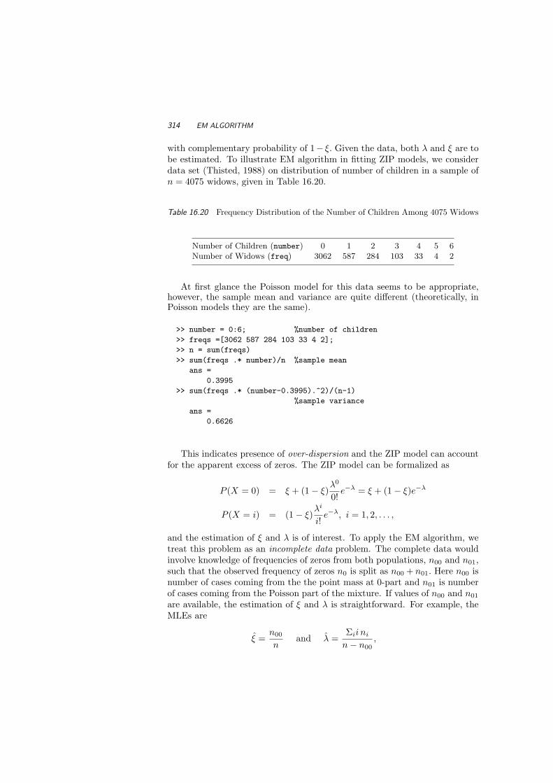
314 EM ALGORITHM
with complementary probability of 1− ξ. Given the data, both λ and ξ are tobe estimated. To illustrate EM algorithm in fitting ZIP models, we considerdata set (Thisted, 1988) on distribution of number of children in a sample ofn = 4075 widows, given in Table 16.20.
Table 16.20 Frequency Distribution of the Number of Children Among 4075 Widows
Number of Children (number) 0 1 2 3 4 5 6Number of Widows (freq) 3062 587 284 103 33 4 2
At first glance the Poisson model for this data seems to be appropriate,however, the sample mean and variance are quite different (theoretically, inPoisson models they are the same).
>> number = 0:6; %number of children
>> freqs =[3062 587 284 103 33 4 2];
>> n = sum(freqs)
>> sum(freqs .* number)/n %sample mean
ans =
0.3995
>> sum(freqs .* (number-0.3995).^2)/(n-1)
%sample variance
ans =
0.6626
This indicates presence of over-dispersion and the ZIP model can accountfor the apparent excess of zeros. The ZIP model can be formalized as
P (X = 0) = ξ + (1− ξ)λ0
0!e−λ = ξ + (1− ξ)e−λ
P (X = i) = (1− ξ)λi
i!e−λ, i = 1, 2, . . . ,
and the estimation of ξ and λ is of interest. To apply the EM algorithm, wetreat this problem as an incomplete data problem. The complete data wouldinvolve knowledge of frequencies of zeros from both populations, n00 and n01,such that the observed frequency of zeros n0 is split as n00 + n01. Here n00 isnumber of cases coming from the the point mass at 0-part and n01 is numberof cases coming from the Poisson part of the mixture. If values of n00 and n01
are available, the estimation of ξ and λ is straightforward. For example, theMLEs are
ξ =n00
nand λ =
Σii ni
n− n00,

EM AND ORDER STATISTICS 315
where ni is the observed frequency of i children. This will be a basis forM -step in the EM implementation, because the estimator of ξ comes fromthe fact that n00 ∼ Bin(n, ξ), while the estimator of λ is the sample meanof the Poisson part. The E-step involves finding En00 if ξ and λ are known.With n00 ∼ Bin(n0, p00/(p00 + p01)), where p00 = ξ and p01 = (1− ξ)e−λ, theexpectation of n00 is
E(n00| observed frequencies, ξ, λ) = n0 × ξ
ξ + (1− ξ)e−λ.
From this expectation, the iterative procedure can be set with
n(t)00 = n0 × ξ(t)
ξ(t) + (1− ξ(t)) exp−λ(t)ξ(t+1) = n
(t)00 /n, and
λ(t+1) =1
n− n(t)00
Σii ni,
where t is the iteration step. The following MATLAB code performs 20 it-erations of the algorithm and collects the calculated values of n00, ξ and λin three sequences newn00s, newxis, and newlambdas. The initial values aregiven for ξ and λ as ξ0 = 3/4 and λ0 = 1/4.
>> newxi =3/4; newlambda = 1/4; %initial values
>> newn00s=[]; newxis=[]; newlambdas=[];
>> for i = 1:20
newn00 = freqs(1) * newxi/(newxi + ...
(1-newxi)*exp(-newlambda) );
newxi = newn00/n;
newlambda = sum((1:6).* freqs(2:7))/(n-newn00);
%collect the values in three sequences
newn00s=[newn00s newn00]; newxis=[newxis newxi];
newlambdas=[newlambdas newlambda];
end
Table 16.21 gives the partial output of the MATLAB program. The valuesfor newxi, newlambda, and newn00 will stabilize after several iteration steps.
16.3 EM AND ORDER STATISTICS
When applying nonparametric maximum likelihood to data that contain (in-dependent) order statistics, the EM Algorithm can be applied by assumingthat with the observed order statistic Xi:k (the ith smallest observation froman i.i.d. sample of k), there are associated with it k − 1 missing values: i− 1values smaller than Xi:k and k−i values that are larger. Kvam and Samaniego(1994) exploited this opportunity to use the EM for finding the nonparametric

316 EM ALGORITHM
Table 16.21 Some of the Twenty Steps in the EM Implementation of ZIP Modelingon Widow Data
Step newxi newlambda newn00
0 1/4 3/4 2430.91 0.5965 0.9902 2447.22 0.6005 1.0001 2460.13 0.6037 1.0081 2470.2...18 0.6149 1.0372 2505.619 0.6149 1.0373 2505.820 0.6149 1.0374 2505.9
MLE for i.i.d. component lifetimes based on observing only k-out-of-n systemlifetimes. Recall a k-out-of-n system needs k or more working components tooperate, and fails after n − k + 1 components fail, hence the system lifetimeis equivalent to Xn−k+1:n.
Suppose we observe independent order statistics Xri:ki , i = 1, . . . , n wherethe unordered values are independently generated from F . When F is abso-lutely continuous, the density for Xri:ki is expressed as
fri:ki(x) = ri
(ki
ri
)F ri−1(x) (1− F (x))ki−ri f(x).
For simplicity, let ki = k. In this application, we assign the completedata to be Xi = Xi1, . . . , Xik, Zi, i = 1, . . . , n where Zi is defined as therank of the value observed from Xi. The observed data can be written asYi = Wi, Zi, where Wi is the Zi
th smallest observation from Xi.With the complete data, the MLE for F (x) is the EDF, which we will write
as N(x)/(nk) where N(x) = ΣiΣj1(Xij ≤ x). This makes the M-step simple,but for the E-step, N is estimated through the log-likelihood. For example, ifZi = z, we observe Wi distributed as Xz:k. If Wi ≤ x, out of the subgroup ofsize k from which Wi was measured,
z + (k − z)F (t)− F (Wi)
1− F (Wi)
are expected to be less than or equal to x. On the other hand, if Wi > x, weknow k − z + 1 elements from Xi are larger than x, and
(z − 1)F (Wi)F (x)
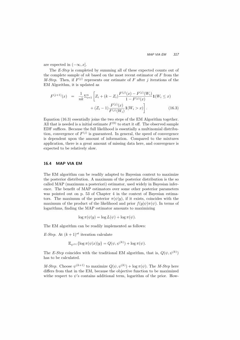
MAP VIA EM 317
are expected in (−∞, x].The E-Step is completed by summing all of these expected counts out of
the complete sample of nk based on the most recent estimator of F from theM-Step. Then, if F (j) represents our estimate of F after j iterations of theEM Algorithm, it is updated as
F (j+1)(x) =1nk
Σni=1
[Zi + (k − Zi)
F (j)(x)− F (j)(Wi)1− F (j)(x)
1(Wi ≤ x)
+ (Zi − 1)F (j)(x)
F (j)(Wi)1(Wi > x)
]. (16.3)
Equation (16.3) essentially joins the two steps of the EM Algorithm together.All that is needed is a initial estimate F (0) to start it off. The observed sampleEDF suffices. Because the full likelihood is essentially a multinomial distribu-tion, convergence of F (j) is guaranteed. In general, the speed of convergenceis dependent upon the amount of information. Compared to the mixturesapplication, there is a great amount of missing data here, and convergence isexpected to be relatively slow.
16.4 MAP VIA EM
The EM algorithm can be readily adapted to Bayesian context to maximizethe posterior distribution. A maximum of the posterior distribution is the socalled MAP (maximum a posteriori) estimator, used widely in Bayesian infer-ence. The benefit of MAP estimators over some other posterior parameterswas pointed out on p. 53 of Chapter 4 in the context of Bayesian estima-tors. The maximum of the posterior π(ψ|y), if it exists, coincides with themaximum of the product of the likelihood and prior f(y|ψ)π(ψ). In terms oflogarithms, finding the MAP estimator amounts to maximizing
log π(ψ|y) = log L(ψ) + log π(ψ).
The EM algorithm can be readily implemented as follows:
E-Step. At (k + 1)st iteration calculate
Eψ(k)log π(ψ|x)|y = Q(ψ, ψ(k)) + log π(ψ).
The E-Step coincides with the traditional EM algorithm, that is, Q(ψ, ψ(k))has to be calculated.
M-Step. Choose ψ(k+1) to maximize Q(ψ, ψ(k)) + log π(ψ). The M-Step herediffers from that in the EM, because the objective function to be maximizedwithe respect to ψ’s contains additional term, logarithm of the prior. How-

318 EM ALGORITHM
ever, the presence of this additional term contributes to the concavity of theobjective function thus improving the speed of convergence.
Example 16.2 MAP Solution to Fisher’s Genomic Example. Assumethat we elicit a Be(ν1, ν2) prior on ψ,
π(ψ) =1
B(ν1, ν2)ψν1−1(1− ψ)ν2−1.
The beta distribution is a natural conjugate for the missing data distribution,because y12 ∼ Bin(y1, (ψ/4)/(1/2 + ψ/4)). Thus the log-posterior (additiveconstants ignored) is
log π(ψ|x) = log L(ψ) + log π(ψ)= (y12 + y4 + ν1 − 1) log ψ + (y2 + y3 + ν2 − 1) log(1− ψ).
The E-step is completed by replacing y12 by its conditional expectationy1 × (ψ(k)/4)/(1/2 + ψ(k)/4). This step is the same as in the standard EMalgorithm.
The M-Step, at (k + 1)st iteration, is
ψ(k+1) =y(k)12 + y4 + ν1 − 1
y(k)12 + y2 + y3 + y4 + ν1 + ν2 − 2
.
When the beta prior coincides with uniform distribution (that is, when ν1 =ν2 = 1), the MAP and MLE solutions coincide.
16.5 INFECTION PATTERN ESTIMATION
Reilly and Lawlor (1999) applied the EM Algorithm to identify contaminatedlots in blood samples. Here the observed data contain the disease exposurehistory of a person over k points in time. For the ith individual, let
Xi = 1(ith person infected by end of trial),
where Pi = P (Xi = 1) is the probability that the ith person was infected atleast once during k exposures to the disease. The exposure history is definedas a vector yi = yi1, . . . , yik, where
yij = 1(ith person exposed to disease at jth time point k).
Let λj be the rate of infection at time point j. The probability of not beinginfected in time point j is 1 − yijλj , so we have Pi = 1 −∏
(1− yijλj). Thecorresponding likelihood for λ = λ1, . . . , λk from observing n patients is a

EXERCISES 319
bit daunting:
L(λ) =n∏
i=1
pxii (1− pi)
1−xi
=n∏
i=1
1−
k∏
j=1
(1− yijλj)
xi
k∏
j=1
(1− yijλj)
1−xi
.
The EM Algorithm helps if we assign the unobservable
Zij = 1(person i infected at time point j),
where P (Zij = 1) = λj if yij=1 and P (Zij = 1) = 0 if yij=0. Averaging overyij , P (Zij = 1) = yijλj . With zij in the complete likelihood (1 ≤ i ≤ n, 1 ≤j ≤ k), we have the observed data changing to xi = maxzi1, . . . , zik, and
L(λ|Z) =n∏
i=1
k∏
j=1
(yijλj)zij (1− yijλj)
1−zij ,
which has the simple binomial form.For the E-Step, we find E(Zij |xi, λ
(m)), where λ(m) is the current estimatefor (λ1, . . . , λk) after m iterations of the algorithm. We need only concernourselves with the case xi = 1, so that
E(Zij |xi = 1) = P (yij = 1|xi = 1) =yijλj
1−∏kj=1 (1− yijλj)
.
In the M-Step, MLEs for (λ1, . . . , λk) are updated in iteration m + 1 fromλ1
(m), . . . , λk(m) to
λj(m+1) =
Σni=1yij
[yijλj
(m+1)
1−Qkj=1(1−yijλj
(m+1))
]
Σni=1yij
.
16.6 EXERCISES
16.1. Suppose we have data generated from a mixture of two normal distri-butions with a common known variance. Write a MATLAB script todetermine the MLE of the unknown means from an i.i.d. sample fromthe mixture by using the EM algorithm. Test your program using asample of ten observations generated from an equal mixture of the twokernels N (0, 1) and N (1, 1).
16.2. The data in the following table come from the mixture of two Poisson

320 EM ALGORITHM
random variables, P(λ1) with probability ε and P(λ2) with probability1− ε.
Value 0 1 2 3 4 5 6 7 8 9 10Freq. 708 947 832 635 427 246 121 51 19 6 1
(i) Develop an EM algorithm for estimating ε, λ1, and λ2.
(ii) Write MATLAB program that uses (i) in estimating ε, λ1, and λ2
for data from the table.
16.3. The following data give the numbers of occupants in 1768 cars observedon a road junction in Jakarta, Indonesia, during a certain time periodon a weekday morning.
Number of occupants 1 2 3 4 5 6 7Number of cars 897 540 223 85 17 5 1
The proposed model for number of occupants X is truncated Poisson(TP), defined as
P (X = i) =λi exp−λ
(1− exp−λ) i!, i = 1, 2, . . .
(i) Write down the likelihood (or the log-likelihood) function. Is itstraightforward to find the MLE of λ by maximizing the likelihood orlog-likelihood directly?
(ii) Develop an EM algorithm for approximating the MLE of λ. Hint:Assume that missing data is i0 – the number of cases when X = 0, sowith the complete data the model is Poisson, P(λ). Estimate λ from thecomplete data. Update i0 given the estimator of λ.
(iii) Write MATLAB program that will estimate the MLE of λ forJakarta cars data using the EM procedure from (ii).
16.4. Consider the problem of right censoring in lifetime measurements inChapter 10. Set up the EM algorithm for solving the nonparametricMLE for a sample of possibly-right censored values X1, . . . , Xn.
16.5. Write MATLAB program that will approximate the MAP estimator inFisher’s problem (Example 16.2), if the prior on ψ is Be(2, 2). Comparethe MAP and MLE solutions.

REFERENCES 321
REFERENCES
Dempster, A. P., Laird, N. M., and Rubin, D. B. (1977), “Maximum Likeli-hood from Incomplete Data via the EM Algorithm” (with discussion),Journal of the Royal Statistical Society, Ser. B, 39, 1-38.
Fisher, R.A. and Balmukand, B. (1928). The estimation of linkage from theoffspring of selfed heterozygotes. Journal of Genetics, 20, 79-92.
Healy M. J. R., and Westmacott M. H. (1956), “Missing Values in ExperimentsAnalysed on Automatic Computers,” Applied Statistics,5, 203-306.
Kvam, P. H., and Samaniego, F. J. (1994) “Nonparametric Maximum Likeli-hood Estimation Based on Ranked Set Samples,” Journal of the Ameri-can Statistical Association, 89, 526-537.
McKendrick, A. G. (1926), “Applications of Mathematics to Medical Prob-lems,” Proceedings of the Edinburgh Mathematical Society, 44, 98-130.
McLachlan, G. J., and Krishnan, T. (1997), The EM Algorithm and Exten-sions, New York: Wiley.
Rao, C. R. (1973), Linear Statistical Inference and its Applications, 2nd ed.,New York: Wiley.
Reilly, M., and Lawlor E. (1999), “A Likelihood Method of Identifying Con-taminated Lots of Blood Product,” International Journal of Epidemiol-ogy, 28, 787-792.
Slatkin, M., and Excoffier, L. (1996), “Testing for Linkage Disequilibriumin Genotypic Data Using the Expectation-Maximization Algorithm,”Heredity, 76, 377-383.
Tsai, W. Y., and Crowley, J. (1985), A Large Sample Study of General-ized Maximum Likelihood Estimators from Incomplete Data via Self-Consistency,” Annals of Statistics, 13, 1317-1334.
Thisted, R. A. (1988), Elements of Statistical Computing: Numerical Com-putation, New York: Chapman & Hall.
Wu, C. F. J. (1983), “On the Convergence Properties of the EM Algorithm,”Annals of Statistics, 11, 95-103.


17Statistical Learning
Learning is not compulsory . . . neither is survival.
W. Edwards Deming (1900–1993)
A general type of artificial intelligence, called machine learning, refers to tech-niques that sift through data and find patterns that lead to optimal decisionrules, such as classification rules. In a way, these techniques allow computersto “learn” from the data, adapting as trends in the data become more clearlyunderstood with the computer algorithms. Statistical learning pertains to thedata analysis in this treatment, but the field of machine learning goes wellbeyond statistics and into algorithmic complexity of computational methods.
In business and finance, machine learning is used to search through hugeamounts of data to find structure and pattern, and this is called data mining.In engineering, these methods are developed for pattern recognition, a term forclassifying images into predetermined groups based on the study of statisticalclassification rules that statisticians refer to as discriminant analysis. In elec-trical engineering, specifically, the study of signal processing uses statisticallearning techniques to analyze signals from sounds, radar or other monitoringdevices and convert them into digital data for easier statistical analysis.
Techniques called neural networks were so named because they were thoughtto imitate the way the human brain works. Analogous to neurons, connectionsbetween processing elements are generated dynamically in a learning systembased on a large database of examples. In fact, most neural network algo-rithms are based on statistical learning techniques, especially nonparametric
323

324 STATISTICAL LEARNING
ones.In this chapter, we will only present a brief exposition of classification and
statistical learning that can be used in machine learning, discriminant anal-ysis, pattern recognition, neural networks and data mining. Nonparametricmethods now play a vital role in statistical learning. As computing power hasprogressed through the years, researchers have taken on bigger and more com-plex problems. An increasing number of these problems cannot be properlysummarized using parametric models.
This research area has a large and growing knowledge base that cannot bejustly summarized in this book chapter. For students who are interested inreading more about statistical learning methods, both parametric and non-parametric, we recommend books by Hastie, Tibshirani and Friedman (2001)and Duda, Hart and Stork (2001).
17.1 DISCRIMINANT ANALYSIS
Discriminant Analysis is the statistical name for categorical prediction. Thegoal is to predict a categorical response variable, G, from one or more predictorvariables, x. For example, if there is a partition of k groups G = (G1, . . . , Gk),we want to find the probability that any particular observation x belongsto group Gj , j = 1, . . . , k and then use this information to classify it inone group or the other. This is called supervised classification or supervisedlearning because the structure of the categorical response is known, and theproblem is to find out in which group each observation belongs. Unsupervisedclassification, or unsupervised learning on the other hand, aims to find outhow many relevant classes there are and then to characterize them.
One can view this simply as a categorical extension to prediction for simpleregression: using a set of data of the form (x1, g1) , . . . , (xn, gn), we want todevise a rule to classify future observations xn+1, . . . , xn+m.
17.1.1 Bias Versus Variance
Recall that a loss function measures the discrepancy between the data re-sponses and what the proposed model predicts for response values, given thecorresponding set of inputs. For continuous response values y with inputs x,we are most familiar with squared error loss
L(y, f) = (y − f(x))2 .
We want to find the predictive function f that minimizes the expected loss,E[L(y, f)], where the expectation averages over all possible response values.With the observed data set, we can estimate this as

DISCRIMINANT ANALYSIS 325
Ef =1n
Σni=1L
(yi, f(xi)
).
The function that minimizes the squared error is the conditional meanE(Y |X = x), and the expected squared errors E(Y − f(Y ))2 consists of twoparts: variance and the square of the bias. If the classifier is based on aglobal rule, such as linear regression, it is simple, rigid, but at least stable. Ithas little variance, but by overlooking important nuances of the data, can behighly biased. A classifier that fits the model locally fails to garner informationfrom as many observations and is more unstable. It has larger variance,but its adaptability to the detailed characteristics of the data ensure it hasless bias. Compared to traditional statistical classification methods, mostnonparametric classifiers tend to be less stable (more variable) but highlyadaptable (less bias).
17.1.2 Cross-Validation
Obviously, the more local model will report less error than a global model,so instead of finding a model that simply minimizes error for the data set, itis better to put aside some of the data to test the model fit independently.The part of the data used to form the estimated model is called the trainingsample. The reserved group of data is the test sample.
The idea of using a training sample to develop a decision rule is paramountto empirical classification. Using the test sample to judge the method con-structed from the training data is called cross-validation. Because data areoften sparse and hard to come by, some methods use the training set to bothdevelop the rule and to measure its misclassification rate (or error rate) aswell. See the jackknife and bootstrap methods described in Chapter 15, forexample.
17.1.3 Bayesian Decision Theory
There are two kinds of loss functions commonly used for categorical responses:a zero-one loss and cross-entropy loss. The zero-one loss merely counts thenumber of misclassified observations. Cross-entropy, on the other hand, usesthe estimated class probabilities pi(x) = P (g ∈ Gi|x)), and we minimizeE(−2 ln pi(X)).
By using zero-one loss, the estimator that minimizes risk classifies theobservation to the most probable class, given the input P (G|X). Becausethis is based on Bayes rule of probability, this is called the Bayes Classi-fier. Although, if P (X|Gi) represents the distribution of observations frompopulation Gi, it might be assumed we know a prior probability P (Gi) that
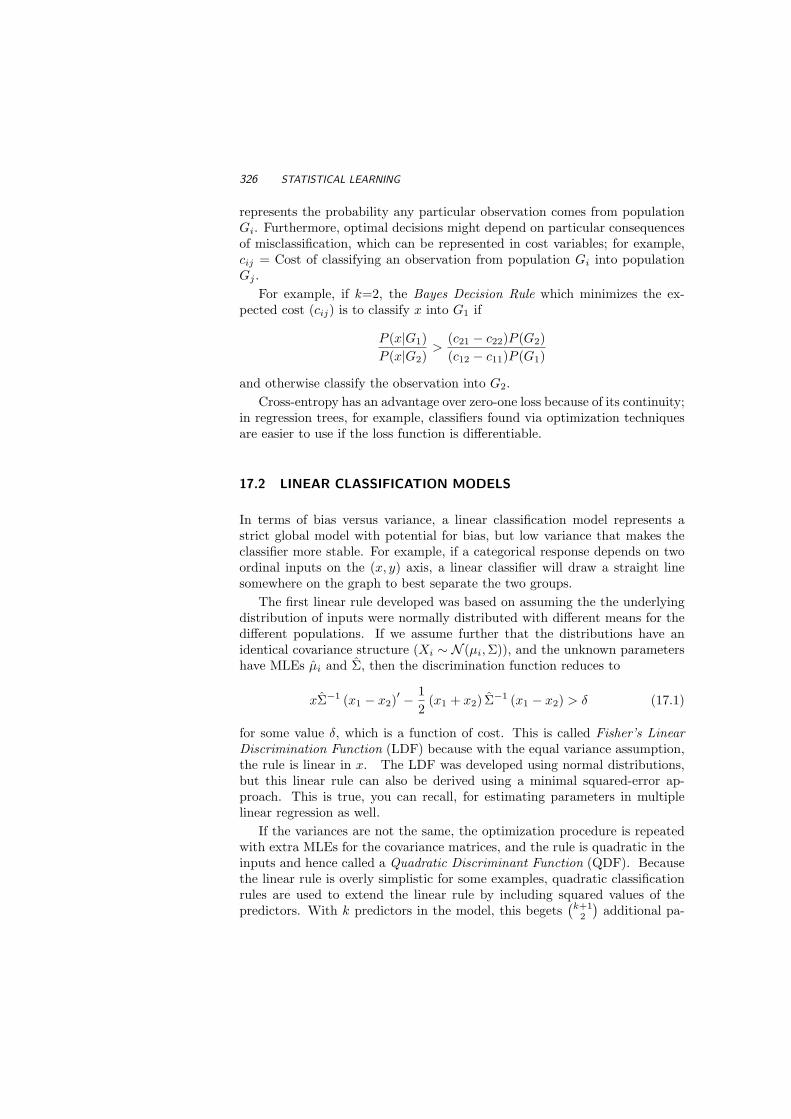
326 STATISTICAL LEARNING
represents the probability any particular observation comes from populationGi. Furthermore, optimal decisions might depend on particular consequencesof misclassification, which can be represented in cost variables; for example,cij = Cost of classifying an observation from population Gi into populationGj .
For example, if k=2, the Bayes Decision Rule which minimizes the ex-pected cost (cij) is to classify x into G1 if
P (x|G1)P (x|G2)
>(c21 − c22)P (G2)(c12 − c11)P (G1)
and otherwise classify the observation into G2.Cross-entropy has an advantage over zero-one loss because of its continuity;
in regression trees, for example, classifiers found via optimization techniquesare easier to use if the loss function is differentiable.
17.2 LINEAR CLASSIFICATION MODELS
In terms of bias versus variance, a linear classification model represents astrict global model with potential for bias, but low variance that makes theclassifier more stable. For example, if a categorical response depends on twoordinal inputs on the (x, y) axis, a linear classifier will draw a straight linesomewhere on the graph to best separate the two groups.
The first linear rule developed was based on assuming the the underlyingdistribution of inputs were normally distributed with different means for thedifferent populations. If we assume further that the distributions have anidentical covariance structure (Xi ∼ N (µi, Σ)), and the unknown parametershave MLEs µi and Σ, then the discrimination function reduces to
xΣ−1 (x1 − x2)′ − 1
2(x1 + x2) Σ−1 (x1 − x2) > δ (17.1)
for some value δ, which is a function of cost. This is called Fisher’s LinearDiscrimination Function (LDF) because with the equal variance assumption,the rule is linear in x. The LDF was developed using normal distributions,but this linear rule can also be derived using a minimal squared-error ap-proach. This is true, you can recall, for estimating parameters in multiplelinear regression as well.
If the variances are not the same, the optimization procedure is repeatedwith extra MLEs for the covariance matrices, and the rule is quadratic in theinputs and hence called a Quadratic Discriminant Function (QDF). Becausethe linear rule is overly simplistic for some examples, quadratic classificationrules are used to extend the linear rule by including squared values of thepredictors. With k predictors in the model, this begets
(k+12
)additional pa-

LINEAR CLASSIFICATION MODELS 327
rameters to estimate. So many parameters in the model can cause obviousproblems, even in large data sets.
There have been several studies that have looked into the quality of linearand quadratic classifiers. While these rules work well if the normality assump-tions are valid, the performance can be pretty lousy if they are not. There arenumerous studies on the LDF and QDF robustness, for example, see Moore(1973), Marks and Dunn (1974), Randles, Bramberg, and Hogg (1978).
17.2.1 Logistic Regression as Classifier
The simple zero-one loss function makes sense in the categorical classificationproblem. If we relied on the squared error loss (and outputs labeled withzeroes and ones), the estimate for g is not necessarily in [0, 1], and even if thelarge sample properties of the procedure are satisfactory, it will be hard totake such results seriously.
One of the simplest models in the regression framework is the logisticregression model, which serves as a bridge between simple linear regressionand statistical classification. Logistic regression, discussed in Chapter 12 inthe context of Generalized Linear Models (GLM), applies the linear model tobinary response variables, relying on a link function that will allow the linearmodel to adequately describe probabilities for binary outcomes. Below wewill use a simple illustration of how it can be used as a classifier. For a morecomprehensive instruction on logistic regression and other models for ordinaldata, Agresti’s book Categorical Data Analysis serves as an excellent basis.
If we start with the simplest case where k = 2 groups, we can arbitrarilyassign gi = 0 or gi = 1 for categories G0 and G1. This means we are modelinga binary response function based on the measurements on x. If we restrictour attention to a linear model P (g = 1|x) = x′β, we will be saddled with anunrefined model that can estimate probability with a value outside [0,1]. Toavoid this problem, consider transformations of the linear model such as
(i) logit: p(x) = P (g = 1|x) = exp(x′β)/[1+ exp(x′β)], so x′β is estimatingln[p(x)/(1− p(x))] which has its range on R.
(ii) probit: P (g = 1|x) = Φ(x′β), where Φ is the standard normal CDF. Inthis case x′β is estimating Φ−1(p(x)).
(iii) log-log: p(x) = 1 − exp(exp(x′β)) so that x′β is estimating ln[− ln(1 −p(x))] on R.
Because the logit transformation is symmetric and has relation to the nat-ural parameter in the GLM context, it is generally the default transformationin this group of three. We focus on the logit link and seek to maximize the

328 STATISTICAL LEARNING
likelihood
L(β) =n∏
i=1
pi(x)gi(1− pi(x))1−gi ,
in terms of p(x) = 1 − exp(exp(x′β)) to estimate β and therefore obtainMLEs for p(x) = P (g = 1|x). This likelihood is rather well behaved and canbe maximized in a straightforward manner. We use the MATLAB functionlogistic to perform a logistic regression in the example below.
Example 17.1 (Kutner, Nachtsheim, and Neter, 1996) A study of 25 com-puter programmers aims to predict task success based on the programmers’months of work experience. The MATLAB m-file logist computes simpleordinal logistic regressions:
>> x=[14 29 6 25 18 4 18 12 22 6 30 11 30 5 20 13 9 32
24 13 19 4 28 22 8];
>> y=[0 0 0 1 1 0 0 0 1 0 1 0 1 0 1 0 0 1 0 1 0 0 1 1 1];
>> logist(y,x,1)
Number of iterations
3
Deviance
25.4246
Theta SE
3.0585 1.2590
Beta SE
0.1614 0.0650
ans =
0.1614
Here β = (β0, β1) and β=(3.0585,0.1614). The estimated logistic regressionfunction is
p =e−3.0585+0.1615x
1 + e−3.0585+0.1615x.
For example, in the case x1 = 14, we have p1 = 0.31; i.e., we estimatethat there is a 31% chance a programmer with 14 months experience willsuccessfully complete the project.
In the logistic regression model, if we use p as a criterion for classifyingobservations, the regression serves as a simple linear classification model. Ifmisclassification penalties are the same for each category, p = 1/2 will be theclassifier boundary. For asymmetric loss, the relative costs of the misclassifi-cation errors will determine an optimal threshold.
Example 17.2 (Fisher’s Iris Data) To illustrate this technique, we use Fisher’sIris data, which is commonly used to show off classification methods. The irisdata set contains physical measurements of 150 flowers – 50 for each of three

NEAREST NEIGHBOR CLASSIFICATION 329
types of iris (Virginica, Versicolor and Setosa). Iris flowers have three petalsand three outer petal-like sepals. Figure (17.2.1a) shows a plot of petal lengthvs width for Versicolor (circles) and Virginica (plus signs) along with the linethat best linearly categorizes them. How is this line determined?
From the logistic function x′β = ln(p/(1 − p)), p = 1/2 represents anobservation that is half-way between the Virginica iris and the Versicolor iris.Observations with values of p < 0.5 are classified to be Versicolor while thosewith p > 0.5 are classified as Virginica. At p = 1/2, x′β = ln(p/(1− p)) = 0,and the line is defined by β0 + β1x1 + β2x2 = 0, which in this case equates tox2 = (42.2723− 5.7545x1)/10.4467. This line is drawn in Figure (17.2.1a).
>> load iris
>> x = [PetalLength,PetalWidth];
>> plot(PetalLength(51:100), PetalWidth(51:100),’o’)
>> hold on
>> x2 = [PetalLength(51:150), PetalWidth(51:150)];
>> fplot(’(45.27-5.7*x)/10.4’,[3,7])
>> v2 = Variety(51:150);
>> L2 = logist(v2,x2,1);
Number of iterations
8
Deviance
20.5635
Theta SE
45.2723 13.6117
Beta SE
5.7545 2.3059
10.4467 3.7556
While this example provides a spiffy illustration of linear classification,most populations are not so easily differentiated, and a linear rule can seemoverly simplified and crude. Figure (17.2.1b) shows a similar plot of sepalwidth vs. length. The iris types are not so easily distinguished, and the linearclassification does not help us in this example.
In the next parts of this chapter, we will look at “nonparametric” classify-ing methods that can be used to construct a more flexible, nonlinear classifier.
17.3 NEAREST NEIGHBOR CLASSIFICATION
Recall from Chapter 13, nearest neighbor methods can be used to createnonparametric regressions by determining the regression curve at x based onexplanatory variables xi that are considered closest to x. We will call this ak-nearest neighbor classifier if it considers the k closest points to x (using amajority vote) when constructing the rule at that point.
If we allow k to increase, the estimator eventually uses all of the data to

330 STATISTICAL LEARNING
3 3.5 4 4.5 5 5.5 6 6.5 71
1.5
2
2.5
4.5 5 5.5 6 6.5 7 7.5 82
2.2
2.4
2.6
2.8
3
3.2
3.4
3.6
3.8
(a) (b)
Fig. 17.1 Two types of iris classified according to (a) petal length vs. petal width,and (b) sepal length vs. sepal width. Versicolor = o, Virginica = +.
fit each local response, so the rule is a global one. This leads to a simplermodel with low variance. But if the assumptions of the simple model arewrong, high bias will cause the expected mean squared error to explode. Onthe other hand, if we let k go down to one, the classifier will create minuteneighborhoods around each observed xi, revealing nothing from the data thata plot of the data has not already shown us. This is highly suspect as well.
The best model is likely to be somewhere in between these two extremes.As we allow k to increase, we will receive more smoothness in the classificationboundary and more stability in the estimator. With small k, we will have amore jagged classification rule, but the rule will be able to identify moreinteresting nuances of the data. If we use a loss function to judge which isbest, the 1-nearest neighbor model will fit best, because there is no penaltyfor over-fitting. Once we identify each estimated category (conditional on X)as the observed category in the data, there will be no error to report.
In this case, it will help to split the data into a training sample and atest sample. Even with the loss function, the idea of local fitting workswell with large samples. In fact, as the input sample size n gets larger, thek-nearest neighbor estimator will be consistent as long as k/n → 0. Thatis, it will achieve the goals we wanted without the strong model assumptionsthat come with parametric classification. There is an extra problem using thenonparametric technique, however. If the dimension of X is somewhat large,the amount of data needed to achieve a satisfactory answer from the nearestneighbor grows exponentially.

NEAREST NEIGHBOR CLASSIFICATION 331
17.3.1 The Curse of Dimensionality
The curse of dimensionality, termed by Bellman (1961), describes the prop-erty of data to become sparse if the dimension of the sample space increases.For example, imagine the denseness of a data set with 100 observations dis-tributed uniformly on the unit square. To achieve the same denseness in a10-dimensional unit hypercube, we would require 1020 observations.
This is a significant problem for nonparametric classification problemsincluding nearest neighbor classifiers and neural networks. As the dimen-sion of inputs increase, the observations in the training set become relativelysparse. These procedures based on a large number of parameters help to han-dle complex problems, but must be considered inappropriate for most small ormedium sized data sets. In those cases, the linear methods may seem overlysimplistic or even crude, but still preferable to nearest neighbor methods.
17.3.2 Constructing the Nearest Neighbor Classifier
The classification rule is based on the ratio of the nearest-neighbor densityestimator. That is, if x is from population G, then P (x|G) ≈ (proportion ofobservations in the neighborhood around x)/(volume of the neighborhood).To classify x, select the population corresponding to the largest value of
P (Gi)P (x|Gi)ΣjP (Gj)P (x|Gj)
, i = 1, . . . , k.
This simplifies to the nearest neighbor rule; if the neighborhood around x isdefined to be the closest r observations, x is classified into the population thatis most frequently represented in that neighborhood.
Figure (17.4) shows the output derived from the MATLAB example below.Fifty randomly generated points are classified into one of two groups in v ina partially random way. The nearest neighbor plots reflect three differentsmoothing conditions of k=11, 5 and 1. As k gets smaller, the classifier actsmore locally, and the rule appears more jagged.
>> y=rand(50,2)
>> v=round(0.3*rand(50,1)+0.3*y(:,1)+0.4*y(:,2));
>> n=100;
>> x=nby2(n);
>> m=n^2;
>> for i=1:m
w(i,1)=nearneighbor(x(i,1:2),y,4,v);
end
>> rr=find(w==1);
>> x2=x(rr,:);
>> plot(x2(:,1),x2(:,2),’.’)

332 STATISTICAL LEARNING
0 5 10 15 20 25 300
0.1
0.2
0.3
0.4
0.5
0.6
0.7
0.8
0.9
1
0.3 0.4 0.5 0.6 0.7 0.8 0.9 10.1
0.2
0.3
0.4
0.5
0.6
0.7
0.8
0.9
1
(a) (b)
0.2 0.3 0.4 0.5 0.6 0.7 0.8 0.9 10
0.1
0.2
0.3
0.4
0.5
0.6
0.7
0.8
0.9
1
0 0.1 0.2 0.3 0.4 0.5 0.6 0.7 0.8 0.9 10
0.1
0.2
0.3
0.4
0.5
0.6
0.7
0.8
0.9
1
(c) (d)
Fig. 17.2 Nearest neighbor classification of 50 observations plotted in (a) using neigh-borhood sizes of (b) 11, (c) 5, (d) 1.

NEURAL NETWORKS 333
17.4 NEURAL NETWORKS
Despite what your detractors say, you have a remarkable brain. Even withthe increasing speed of computer processing, the much slower human brainhas surprising ability to sort through gobs of information, disseminate someof its peculiarities and make a correct classification often several times fasterthan a computer. When a familiar face appears to you around a street corner,your brain has several processes working in parallel to identify this person yousee, using past experience to gauge your expectation (you might not believeyour eyes, for example, if you saw Elvis appear around the corner) along withall the sensory data from what you see, hear, or even smell.
The computer is at a disadvantage in this contest because despite all of thespeed and memory available, the static processes it uses cannot parse throughthe same amount of information in an efficient manner. It cannot adapt andlearn as the human brain does. Instead, the digital processor goes throughsequential algorithms, almost all of them being a waste of CPU time, ratherthan traversing a relatively few complex neural pathways set up by our pastexperiences.
Rosenblatt (1962) developed a simple learning algorithm he named theperceptron, which consists of an input layer of several nodes that is completelyconnected to nodes of an output layer. The perceptron is overly simplistic andhas numerous shortcomings, but it also represents the first neural network.By extending this to a two-step network which includes a hidden layer ofnodes between the inputs and outputs, the network overcomes most of thedisadvantages of the simpler map. Figure (17.4) shows a simple feed-forwardneural network, that is, the information travels in the direction from input tooutput.
Fig. 17.3 Basic structure of feed-forward neural network.
The square nodes in Figure (17.4) represent neurons, and the connections
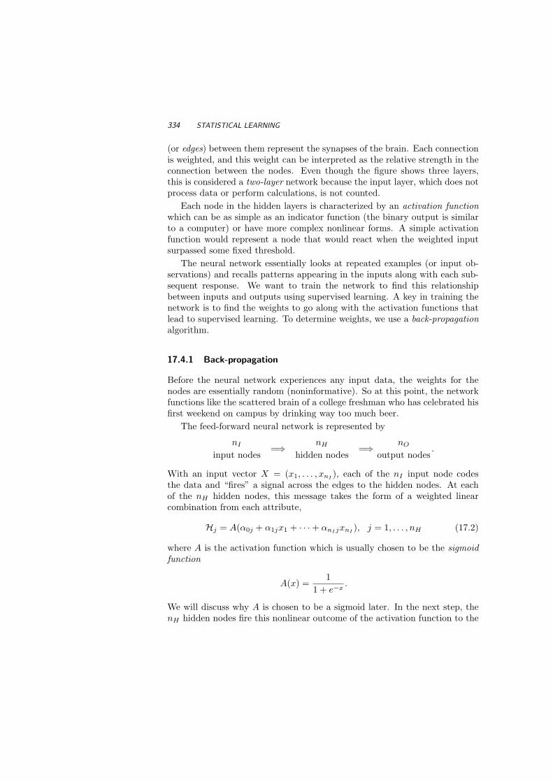
334 STATISTICAL LEARNING
(or edges) between them represent the synapses of the brain. Each connectionis weighted, and this weight can be interpreted as the relative strength in theconnection between the nodes. Even though the figure shows three layers,this is considered a two-layer network because the input layer, which does notprocess data or perform calculations, is not counted.
Each node in the hidden layers is characterized by an activation functionwhich can be as simple as an indicator function (the binary output is similarto a computer) or have more complex nonlinear forms. A simple activationfunction would represent a node that would react when the weighted inputsurpassed some fixed threshold.
The neural network essentially looks at repeated examples (or input ob-servations) and recalls patterns appearing in the inputs along with each sub-sequent response. We want to train the network to find this relationshipbetween inputs and outputs using supervised learning. A key in training thenetwork is to find the weights to go along with the activation functions thatlead to supervised learning. To determine weights, we use a back-propagationalgorithm.
17.4.1 Back-propagation
Before the neural network experiences any input data, the weights for thenodes are essentially random (noninformative). So at this point, the networkfunctions like the scattered brain of a college freshman who has celebrated hisfirst weekend on campus by drinking way too much beer.
The feed-forward neural network is represented by
nI
input nodes=⇒ nH
hidden nodes=⇒ nO
output nodes.
With an input vector X = (x1, . . . , xnI), each of the nI input node codes
the data and “fires” a signal across the edges to the hidden nodes. At eachof the nH hidden nodes, this message takes the form of a weighted linearcombination from each attribute,
Hj = A(α0j + α1jx1 + · · ·+ αnIjxnI), j = 1, . . . , nH (17.2)
where A is the activation function which is usually chosen to be the sigmoidfunction
A(x) =1
1 + e−x.
We will discuss why A is chosen to be a sigmoid later. In the next step, thenH hidden nodes fire this nonlinear outcome of the activation function to the

NEURAL NETWORKS 335
output nodes, each translating the signals as a linear combination
Ok = β0 + β1H1 + · · ·+ βnHHnH , k = 1, . . . , nO. (17.3)
Each output node is a function of the inputs, and through the steps of theneural network, each node is also a function of the weights α and β. If weobserve Xl = (x1l, . . . , xnI l) with output gl(k) for k = 1, . . . , nO, we use thesame kind of transformation used in logistic regression:
gl(k) =eHk
eH1 + eH2 + · · ·+ eHno, k = 1, ..., nO.
For the training data (X1, g1), . . . , (Xn, gn), the classification is com-pared to the observation’s known group, which is then back-propagated acrossthe network, and the network responds (learns) by adjusting weights in thecases an error in classification occurs. The loss function associated with mis-classification can be squared errors, such as
SSQ(α, β) = Σnl=1Σ
nO
k=1(gl(k)− gl(k))2, (17.4)
where gl(k) is the actual response of the input Xl for output node k and gl(k)is the estimated response.
Now we look how those weights are changed in this back-propagation. Tominimize the squared error SSQ in (17.4) with respect to weights α and βfrom both layers of the neural net, we can take partial derivatives (with respectto weight) to find the direction the weights should go in order to decrease theerror. But there are a lot of parameters to estimate: αij , with 1 ≤ i ≤ nI ,1 ≤ j ≤ nH and βjk, 1 ≤ j ≤ nH , 1 ≤ k ≤ nO. It’s not helpful to think ofthis as a parameter set, as if they have their own intrinsic value. If you do,the network looks terribly over-parameterized and unnecessarily complicated.Remember that α and β are artificial, and our focus is on the n predictedoutcomes instead of estimated parameters. We will do this iteratively usingbatch learning by updating the network after the entire data set is entered.
Actually, finding the global minimum of SSQ with respect to α and β willlead to over-fitting the model, that is, the answer will not represent the trueunderlying process because it is blindly mimicking every idiosyncrasy of thedata. The gradient is expressed here with a constant γ called the learningrate:
∆αij = γΣnl=1
∂(ΣnO
k=1(gl(k)− gl(k))2)∂αij
(17.5)
∆βjk = γΣnl=1
∂(ΣnO
k=1(gl(k)− gl(k))2)∂βjk
(17.6)
and is solved iteratively with the following back-propagation equations (see
336 STATISTICAL LEARNING
Chapter 11 of Hastie et al. (2001)) via error variables a and b:
ail =[∂A(t)∂(t)
]
t=α′iXl
Σnl=1βjkbjl. (17.7)
Obviously, the activation function A must be differentiable. Note that if A(x)is chosen as a binary function such as I(x ≥ 0), we end up with a regularlinear model from (17.2). The sigmoid function, when scaled as Ac(x) = A(cx)will look like I(x ≥ 0) as c → ∞, but the function also has a well-behavedderivative.
In the first step, we use current values of α and β to predict outputs from(17.2) and (17.3). In the next step we compute errors b from the output layer,and use (17.7) to compute a from the hidden layer. Instead of batch process-ing, updates to the gradient can be made sequentially after each observation.In this case, γ is not constant, and should decrease to zero as the iterationsare repeated (this is why it is called the learning rate).
The hidden layer of the network, along with the nonlinear activation func-tion, gives it the flexibility to learn by creating convex regions for classificationthat need not be linearly separable like the more simple linear rules require.One can introduce another hidden layer that in effect can allow non convexregions (by combining convex regions together). Applications exist with evenmore hidden layers, but two hidden layers should be ample for almost everynonlinear classification problem that fits into the neural network framework.
17.4.2 Implementing the Neural Network
Implementing the steps above into a computer algorithm is not simple, nor isit free from potential errors. One popular method for processing through theback-propagation algorithm uses six steps:
1. Assign random values to the weights.
2. Input the first pattern to get outputs to the hidden layer (H1, ...,HnH )and output layer (g(1), ..., g(k)).
3. Compute the output errors b.
4. Compute the hidden layer errors a as a function of b.
5. Update the weights using (17.5)
6. Repeat the steps for the next observation
Computing a neural network from scratch would be challenging for manyof us, even if we have a good programming background. In MATLAB,

NEURAL NETWORKS 337
there are a few modest programs that can be used for classification, suchas softmax(X,K,Prior) that uses implements a feed-forward neural networkusing a training set X, a vector K for class indexing, with an optional priorargument. Instead of minimizing SSQ in (17.4), softmax assumes that “theoutputs are a Poisson process conditional on their sum and calculates theerror as the residual deviance.”
MATLAB also has a Neural Networks Toolbox, see
http://www.mathworks.com
which features a graphical user interface (GUI) for creating, training, andrunning neural networks.
17.4.3 Projection Pursuit
The technique of Projection Pursuit is similar to that of neural networks, asboth employ a nonlinear function that is applied only to linear combinationsof the input. While the neural network is relatively fixed with a set numberof hidden layer nodes (and hence a fixed number of parameters), projectionpursuit seems more nonparametric because it uses unspecified functions in itstransformations. We will start with a basic model
g(X) = ΣnPi=1ψ (θ′iX) , (17.8)
where nP represents the number of unknown parameter vectors (θ1, . . . , θnp).Note that θ′iX is the projection of X onto the vector θi. If we pursue a
value of θi that makes this projection effective, it seems logical enough to callthis projection pursuit. The idea of using a linear combination of inputs touncover structure in the data was first suggested by Kruskal (1969). Friedmanand Stuetzle (1981) derived a more formal projection pursuit regression usinga multi-step algorithm:
1. Define τ(0)i = gi.
2. Maximize the standardized squared errors
SSQ(j) = 1−Σn
i=1
(τ
(j−1)i − g(j−1)(w(j)′xi)
)2
Σni=1
(τ
(j−1)i
)2 (17.9)
over weights w(j) (under the constraint that w(j)′1 = 1) and g(j−1).
3. Update τ with τ(j)i = τ
(j−1)i − g(j−1)(w(j)′xi).
4. Repeat the first step k times until SSQ(k) ≤ δ for some fixed δ > 0.

338 STATISTICAL LEARNING
Once the algorithm finishes, it essentially has given up trying to find otherprojections, and we complete the projection pursuit estimator as
g(x) = ΣnPj=1g
(j)(w(j)′x). (17.10)
17.5 BINARY CLASSIFICATION TREES
Binary trees offer a graphical and logical basis for empirical classification. De-cisions are made sequentially through a route of branches on a tree - everytime a choice is made, the route is split into two directions. Observationsthat are collected at the same endpoint (node) are classified into the samepopulation. At those junctures on the route where the split is made are non-terminal nodes, and terminal nodes denote all the different endpoints wherea classification of the tree. These endpoints are also called the leaves of thetree, and the starting node is called the root.
With the training set (x1, g1), . . . , (xn, gn), where x is a vector of m compo-nents, splits are based on a single variable of x, possibly a linear combination.This leads to decision rules that are fairly easy to interpret and explain, sobinary trees are popular for disseminating information to a broad audience.The phases of of tree construction include
• Deciding whether to make the node a terminal node.
• Selection of splits in a nonterminal node
• Assigning classification rule at terminal nodes.
This is the essential approach of CART (Classification and Regression Trees).The goal is to produce a simple and effective classification tree without anexcess number of nodes.
If we have k populations G1, . . . , Gk, we will use the frequencies found inthe training data to estimate population frequency in the same way we con-structed nearest-neighbor classification rules: the proportion of observationsin training set from the ith population = P (Gi) = ni/n. Suppose there areni(r) observations from Gi that reach node r. The probability of such anobservation reaching node r is estimated as
Pi(t) = P (Gi)P (reach node r | Gi) =ni
n× ni(r)
ni=
ni(r)n
.
We want to construct a perfectly pure split where we can isolate one orsome of the populations into a single node that can be a terminal node (or atleast split more easily into one during a later split). Figure 17.4 illustrates a

BINARY CLASSIFICATION TREES 339
n1(r)n2(r)
n1(r)0
0n2(r)
¡¡
¡ª
@@
@R
Fig. 17.4 Purifying a tree by splitting.
perfect split of node r. This, of course, is not always possible. This qualitymeasure of a split is defined in an impurity index function
I(r) = ψ (P1(r), . . . , Pk(r)) ,
where ψ is nonnegative, symmetric in its arguments, maximized at (1/k, . . . , 1/k),and minimized at any k-vector that has a one and k − 1 zeroes.
Several different methods of impurity have been defined for constructingtrees. The three most popular impurity measures are cross-entropy, Giniimpurity and misclassification impurity:
1. Cross-entropy: I(r) = −Σi:Pi(r)>0Pi(r) ln[Pi(r)].
2. Gini: I(r) = −Σi 6=jPi(r)Pj(r).
3. Misclassification: I(r) = 1−maxj Pj(r)
The misclassification impurity represents the minimum probability thatthe training set observations would be (empirically) misclassified at node r.The Gini measure and Cross-entropy measure have an analytical advantageover the discrete impurity measure by being differentiable. We will focus onthe most popular index of the three, which is the cross-entropy impurity.
By splitting a node, we will reduce the impurity to
q(L)I(rL) + q(R)I(rR),
where q(R) is the proportion of observations that go to node rR, and q(L) isthe proportion of observations that go to node rL. Constructed this way, thebinary tree is a recursive classifier.
Let Q be a potential split for the input vector x. If x = (x1, ..., xm),Q = xi > x0 would be a valid split if xi is ordinal, or Q = xi ∈ S ifxi is categorical and S is a subset of possible categorical outcomes for xi. Ineither case, the split creates two additional nodes for the binary response ofthe data to Q. For the first split, we find the split Q1 that will minimize theimpurity measure the most. The second split will be chosen to be the Q2 thatminimizes the impurity from one of the two nodes created by Q1.

340 STATISTICAL LEARNING
Suppose we are the middle of constructing a binary classification tree Tthat has a set of terminal nodes R. With
P ( reach node r) = P (r) = ΣPi(r),
suppose the current impurity function is
IT = Σr∈RI(r)P (r).
At the next stage, then, we split the node that will most greatly decrease IT .
Example 17.3 The following made-up example was used in Elsner, Lehmiller,and Kimberlain (1996) to illustrate a case for which linear classification modelsfail and binary classification trees perform well. Hurricanes categorized ac-cording to season as “tropical only” or “baroclinically influenced”. Hurricanesare classified according to location (longitude, latitude), and Figure (17.5(a))shows that no linear rule can separate the two categories without a greatamount of misclassification. The average latitude of origin for tropical-onlyhurricanes is 18.8oN, compared to 29.1oN for baroclinically influenced storms.The baroclinically influenced hurricane season extends from-mid May to De-cember, while the tropical-only season is largely confined to the months ofAugust through October.
For this problem, simple splits are considered and the ones that minimizeimpurity are Q1 : Longitude ≥ 67.75, and Q2 : Longitude ≤ 62.5 (see home-work). In this case, the tree perfectly separates the two types of storms withtwo splits and three terminal nodes in Figure 17.5(b).
58 60 62 64 66 68 70 7212
13
14
15
16
17
18
19
20
21
(a) (b)
Fig. 17.5 (a) Location of 37 tropical (circles) and other (plus-signs) hurricanes fromElsner at al. (1996); (b) Corresponding separating tree.

BINARY CLASSIFICATION TREES 341
>> long =[59.00 59.50 60.00 60.50 61.00 61.00 61.50 61.50 62.00 63.00...
63.50 64.00 64.50 65.00 65.00 65.00 65.50 65.50 65.50 66.00 66.00...
66.00 66.50 66.50 66.50 67.00 67.50 68.00 68.50 69.00 69.00 69.50...
69.50 70.00 70.50 71.00 71.50];
>> lat = [17.00 21.00 12.00 16.00 13.00 15.00 17.00 19.00 14.00 15.00...
19.00 12.00 16.00 12.00 15.00 17.00 16.00 19.00 21.00 13.00 14.00...
17.00 17.00 18.00 21.00 14.00 18.00 14.00 18.00 13.00 15.00 17.00...
19.00 12.00 16.00 17.00 21.00];
>> trop = [0 0 0 0 0 0 0 0 0 1 1 1 1 1 1 1 1 1 1 1 1 1 1 1 1 1 1 0 0...
0 0 0 0 0 0 0 0];
>> plot(long(find(long’.*trop’>0.5))’,lat(find(long’.*trop’>0.5))’,’o’)
>> hold on
>> plot(long(find(long’.*trop’<0.5))’,lat(find(long’.*trop’<0.5))’,’+’)
17.5.1 Growing the Tree
So far we have not decided how many splits will be used in the final tree; wehave only determined which splits should take place first. In constructing abinary classification tree, it is standard to grow a tree that is initially too large,and to then prune it back, forming a sequence of sub-trees. This approachworks well; if one of the splits made in the tree appears to have no value, itmight be worth saving if there exists below it an effective split.
In this case we define a branch to be a split direction that begins at a nodeand includes all the subsequent nodes in the direction of that split (called asubtree or descendants). For example, suppose we consider splitting tree T atnode r and Tr represents the classification tree after the split is made. Thenew nodes made under r will be denoted rR and rL. The impurity is now
ITr = Σs∈T,s 6=rIT (s)P (s) + P (rR)IT (rR) + P (rL)I(rL).
The change in impurity caused by the split is
∆ITr (r) = P (r)IT (r)− P (rR)IT (rR)− P (rL)IT (rL)
= P (r)(IT (r)− P (rR)
P (rR)IT (rR)− P (rL)
P (rL)IT (rL)
).
Again, let R be the set of all terminal nodes of the tree. If we consider thepotential differences for any particular split Q, say ∆ITr (r; Q), then the nextsplit should be chosen by finding the terminal node r and split Q correspondingto
maxr∈R
(P (r)
(max
Q∆ITr (r; Q)
)).
To prevent the tree from splitting too much, we will have a fixed thresholdlevel τ > 0 so that splitting must stop once the change no longer exceeds τ .

342 STATISTICAL LEARNING
We classify each terminal node according to majority vote: observations interminal node r are classified into the population i with the highest ni(r).With this simple rule, the misclassification rate for observations arriving atnode r is estimated as 1− Pi(r).
17.5.2 Pruning the Tree
With a tree constructed using only a threshold value to prevent overgrowth, alarge set of training data may yield a tree with an abundance of branches andterminal nodes. If τ is small enough, the tree will fit the data locally, similarto how a 1-nearest-neighbor overfits a model. If τ is too large, the tree willstop growing prematurely, and we might fail to find some interesting featuresof the data. The best method is to grow the tree a bit too much and thenprune back unnecessary branches.
To make this efficable, there must be a penalty function ζT = ζT (|R|)for adding extra terminal nodes, where |R| is the cardinality, or number ofterminal nodes of R. We define our cost function to be a combination ofmisclassification error and penalty for over-fitting:
C(T ) = LT + ζT ,
where
LT = Σr∈RP (r)(
1−maxj
Pj(r))≡ Σr∈RLT (r).
This is called the cost-complexity pruning algorithm in Breiman et al(1984). Using this rule, we will always find a subtree of T that minimizesC(T ). If we allow ζT → 0, the subtree is just the original tree T , and if weallow ζT → ∞, the subtree is a single node that doesn’t split at all. If weincrease ζT from 0, we will get a sequence of subtrees, each one being nestedin the previous one.
In deciding whether or not to prune a branch of the tree at node r, we willcompare C(T ) of the tree to the new cost that would result from removing thebranches under node r. LT will necessarily increase, while ζT will decrease asthe number of terminal nodes in the tree decreases.
Let Tr be the branch under node r, so the tree remaining after cuttingbranch Tr (we will call this T(r)) is nested in T , i.e., T(r) ⊂ T . The set ofterminal nodes in the branch Tr is denoted Rr. If another branch at node sis pruned, we will denote the remaining subtree as T(r,s) ⊂ T(r) ⊂ T . Now,
C(Tr) = Σs∈RrLTr (s) + ζTr

BINARY CLASSIFICATION TREES 343
is equal to C(T ) if ζT is set to
h(r) =LT − Σs∈Rr
LTr(s)
|Rr| .
Using this approach, we want to trim the node r that minimizes h(r).Obviously, only non-terminal nodes r ∈ RC because terminal nodes have nobranches. If we repeat this procedure after recomputing h(r) for the resultingsubtree, this pruning will create another sequence of nested trees
T ⊃ T(r1) ⊃ T(r1,r2) ⊃ · · · ⊃ r0,
where r0 is the the first node of the original tree T . Each subtree has anassociated cost (C(T ), C(Tr1), · · · , C(r0)) which can be used to determine atwhat point the pruning should finish. The problem with this procedure isthat the misclassification probability is based only on the training data.
A better estimator can be constructed by cross-validation. If we dividethe training data into ν subsets S1, . . . , Sν , we can form ν artificial trainingsets as
S(j) ≡⋃
i 6=j
Si
and constructing a binary classification tree based on each of the ν setsS(1), · · · , S(ν). This type of cross-validation is analogous to the jackknife“leave-one-out” resampling procedure. If we let L(j) be the estimated misclas-sification probability based on the subtree chosen in the jth step of the crossvalidation (i.e., leaving out Sj), and let ζ(j) be the corresponding penaltyfunction, then
LCV ≡ 1n
Σνj=1L
(j)
provides a bona fide estimator for misclassification error. The correspondingpenalty function for LCV is estimated as the geometric mean of the penaltyfunctions in the cross validation. That is,
ζCV = ν
√√√√ν∏
j=1
ζ(j).
To perform a binary tree search in MATLAB, the function treefit createsa decision tree based on an input an nxm matrix of inputs and a n-vectory of outcomes. The function treedisp creates a graphical representationof the tree using the same inputs. Several options are available to controltree growth, tree pruning, and misclassification costs (see Chapter 23). Thefunction treeprune produces a sequence of trees by pruning according to a

344 STATISTICAL LEARNING
threshold rule. For example, if T is the output of a treeprune function, thentreeprune(T) generates an unpruned tree of T and adds information aboutoptimal pruning.
>> numobs = size(meas,1);
>> tree = treefit(meas(:,1:2), species);
>> [dtnum,dtnode,dtclass] = treeval(tree, meas(:,1:2));
>> bad = ~strcmp(dtclass,species);
>> sum(bad) / numobs
ans =
0.1333
%The decision tree misclassifies 13.3% or 20 of the specimens.
>> [grpnum,node,grpname] = treeval(tree, [x y]);
>> gscatter(x,y,grpname,’grb’,’sod’)
>> treedisp(tree,’name’,’SL’ ’SW’)
>> resubcost = treetest(tree,’resub’);
>> [cost,secost,ntermnodes,bestlevel] = ...
>> treetest(tree,’cross’,meas(:,1:2),species);
>> plot(ntermnodes,cost,’b-’, ntermnodes,resubcost,’r--’)
>> xlabel(’Number of terminal nodes’)
>> ylabel(’Cost(misclassification error)’)
>> legend(’Cross-validation’,’Resubstitution’)
Fig. 17.6 MATLAB function treedisp applied to Fisher’s Iris Data.

BINARY CLASSIFICATION TREES 345
17.5.3 General Tree Classifiers
Classification and regression trees can be conveniently divided to five differentfamilies.
(i) The CART family : Simple versions of CART have been emphasized inthis chapter. This method is characterized by its use of two branchesfrom each nonterminal node. Cross-validation and pruning are used todetermine size of tree. Response variable can be quantitative or nominal.Predictor variables can be nominal or ordinal, and continuous predictorsare supported. Motivation: statistical prediction.
(ii) The CLS family: These include ID3, originally developed by Quinlan(1979), and off-shoots such as CLS and C4.5. For this method, the num-ber of branches equals the number of categories of the predictor. Onlynominal response and predictor variables are supported in early versions,so continuous inputs had to be binned. However, the latest version ofC4.5 supports ordinal predictors. Motivation: concept learning.
(iii) The AID family: Methods include AID, THAID, CHAID, MAID, XAID,FIRM, and TREEDISC. The number of branches varies from two to thenumber of categories of the predictor. Statistical significance tests (withmultiplicity adjustments in the later versions) are used to determine thesize of tree. AID, MAID, and XAID are for quantitative responses.THAID, CHAID, and TREEDISC are for nominal responses, althoughthe version of CHAID from Statistical Innovations, distributed by SPSS,can handle a quantitative categorical response. FIRM comes in two vari-eties for categorical or continuous response. Predictors can be nominalor ordinal and there is usually provision for a missing-value category.Some versions can handle continuous predictors, others cannot. Moti-vation: detecting complex statistical relationships.
(iv) Linear combinations: Methods include OC1 and SE-Trees. The Num-ber of branches varies from two to the number of categories of predictor.Motivation: Detecting linear statistical relationships combined to con-cept learning.
(v) Hybrid models: IND is one example. IND combines CART and C4 aswell as Bayesian and minimum encoding methods. Knowledge Seekercombines methods from CHAID and ID3 with a novel multiplicity ad-justment.Motivation: Combines methods from other families to find op-timal algorithm.

346 STATISTICAL LEARNING
17.6 EXERCISES
17.1. Create a simple nearest-neighbor program using MATLAB. It shouldinput a training set of data in m+1 columns; one column should containthe population identifier 1, ..., k and the others contain the input vectorsthat can have length m. Along with this training set, also input anotherm column matrix representing the classification set. The output shouldcontain n, m, k and the classifications for the input set.
17.2. For the Example 17.3, show the optimal splits, using the cross-entropymeasure, in terms of intervals longitude ≥ l0 and latitude ≥ l1
17.3. In this exercise the goal is to discriminate between observations comingfrom two different normal populations, using logistic regression.
Simulate a training data set, (Xi, Yi), i = 1, . . . , n, (take n even) asfollows: For the first half of data, Xi, i = 1, . . . , n/2 are sampled fromthe standard normal distribution and Yi = 0, i = 1, . . . , n/2. For thesecond half, Xi, i = n/2+1, . . . , n are sampled from normal distributionwith mean 2 and variance 1, while Yi = 1, i = n/2 + 1, . . . , n. Fit thelogistic regression to this data, P (Y = 1) = f(X).
Simulate a validation set (X∗j , Y ∗
j ), j = 1, . . . ,m the same way, andclassify these new Y ∗
j ’s as 0 or 1 depending whether f(X∗j ) < 0.5 or
≥ 0.5.
(a) Calculate the error of this logistic regression classifier,
Ln(m) =1m
Σmj=11
(1(f(X∗
j ) > 0.5) 6= Y ∗j
).
In your simulations use n = 60, 200, and 2000 and m = 100.
(b) Can the error Ln(m) be made arbitrarily small by increasing n?
REFERENCES
Agresti, A. (1990), Categorical Data Analysis, New York: Wiley.Bellman, R. E. (1961), Adaptive Control Processes, Princeton, NJ: Princeton
University Press.Breiman, L., Friedman, J., Olshen, R., and Stone, C. (1984), Classification
and Regression Trees, Belmont, CA: Wadsworth.Duda, R. O., Hart, P. E. and Stork, D. G. (2001), Pattern Classification, New
York: Wiley.

REFERENCES 347
Fisher, R. A. (1936), “The Use of Multiple Measurements in Taxonomic Prob-lems,” Annals of Eugenics, 7, 179-188.
Elsner, J. B., Lehmiller, G. S., and Kimberlain, T. B. (1996), “ObjectiveClassification of Atlantic Basin Hurricanes,” Journal of Climate, 9, 2880-2889.
Friedman, J., and Stuetzle, W. (1981), “Projection Pursuit Regression,” Jour-nal of the American Statistical Association, 76, 817-823.
Hastie, T., Tibshirani, R., and Friedman, J. (2001), The Elements of Statis-tical Learning, New York: Springer Verlag.
Kutner, M. A., Nachtsheim, C. J., and Neter, J. (1996), Applied Linear Re-gression Models, 4th ed., Chicago: Irwin.
Kruskal J. (1969), “Toward a Practical Method which Helps Uncover theStructure of a Set of Multivariate Observations by Finding the LinearTransformation which Optimizes a New Index of Condensation,” Statis-tical Computation, New York: Academic Press, pp. 427-440.
Marks, S., and Dunn, O. (1974), “Discriminant Functions when CovarianceMatrices are Unequal,” Journal of the American Statistical Association,69, 555-559.
Moore, D. H. (1973), “Evaluation of Five Discrimination Procedures for Bi-nary Variables,” Journal of the American Statistical Association, 68, 399-404.
Quinlan, J. R. (1979), “Discovering Rules from Large Collections of Examples:A Case Study.” in Expert Systems in the Microelectronics Age, Ed. D.Michie, Edinburgh: Edinburgh University Press.
Randles, R. H., Broffitt, J.D., Ramberg, J. S., and Hogg, R. V. (1978), “Gen-eralized Linear and Quadratic Discriminant Functions Using Robust Es-timates,” Journal of the American Statistical Association, 73, 564-568.
Rosenblatt, R. (1962), Principles of Neurodynamics: Perceptrons and the The-ory of Brain Mechanisms, Washington, DC: Spartan.


18Nonparametric Bayes
Bayesian (bey’ -zhuhn) n. 1. Result of breeding a statistician with aclergyman to produce the much sought honest statistician.
Anonymous
This chapter is about nonparametric Bayesian inference. Understanding thecomputational machinery needed for non-conjugate Bayesian analysis in thischapter can be quite challenging and it is beyond the scope of this text.Instead, we will use specialized software, WinBUGS, to implement complexBayesian models in a user-friendly manner. Some applications of WinBUGShave been discussed in Chapter 4 and an overview of WinBUGS is given inthe Appendix B.
Our purpose is to explore the useful applications of the nonparametric sideof Bayesian inference. At first glance, the term nonparametric Bayes mightseem like an oxymoron; after all, Bayesian analysis is all about introducingprior distributions on parameters. Actually, nonparametric Bayes is oftenseen as a synonym for Bayesian models with process priors on the spaces ofdensities and functions. Dirichlet process priors are the most popular choice.However, many other Bayesian methods are nonparametric in spirit. In addi-tion to Dirichlet process priors, Bayesian formulations of contingency tablesand Bayesian models on the coefficients in atomic decompositions of functionswill be discussed later in this chapter.
349

350 NONPARAMETRIC BAYES
18.1 DIRICHLET PROCESSES
The central idea of traditional nonparametric Bayesian analysis is to draw in-ference on an unknown distribution function. This leads to models on functionspaces, so that the Bayesian nonparametric approach to modeling requires adramatic shift in methodology. In fact, a commonly used technical defini-tion of nonparametric Bayes models involves infinitely many parameters, asmentioned in Chapter 10.
Results from Bayesian inference are comparable to classical nonparametricinference, such as density and function estimation, estimation of mixtures andsmoothing. There are two main groups of nonparametric Bayes methodolo-gies: (1) methods that involve prior/posterior analysis on distribution spaces,and (2) methods in which standard Bayes analysis is performed on a vastnumber of parameters, such as atomic decompositions of functions and den-sities. Although the these two methodologies can be presented in a unifiedway (see Mueller and Quintana, 2005), because of simplicity we present themseparately.
Recall a Dirichlet random variable can be constructed from gamma randomvariables. If X1, . . . , Xn are i.i.d. Gamma(ai, 1), then for Yi = Xi/Σn
j=1Xj ,the vector (Y1, . . . , Yn) has Dirichlet Dir(a1, . . . , an) distribution. The Dirich-let distribution represents a multivariate extension of the beta distribution:Dir(a1, a2) ≡ Be(a1, a2). Also, from Chapter 2, EYi = ai/Σn
j=1aj , EY 2i =
ai(ai + 1)/Σnj=1aj(1 + Σn
j=1aj), and E(Yi Yj) = aiaj/Σnj=1aj(1 + Σn
j=1aj).The Dirichlet process (DP), with precursors in the work of Freedman
(1963) and Fabius (1964), was formally developed by Ferguson (1973, 1974).It is the first prior developed for spaces of distribution functions. The DP
is, formally, a probability measure (distribution) on the space of probabilitymeasures (distributions) defined on a common probability space X . Hence, arealization of DP is a random distribution function.
The DP is characterized by two parameters: (i) Q0, a specific probabilitymeasure on X (or equivalently, G0 a specified distribution function on X ); (ii)α, a positive scalar parameter.
Definition 18.1 (Ferguson, 1973) The DP generates random probability mea-sures (random distributions) Q on X such that for any finite partition B1, . . . , Bk
of X ,
(Q(B1), . . . , Q(Bk)) ∼ Dir(αQ0(B1), . . . , αQ0(Bk)),
where, Q(Bi) (a random variable) and Q0(Bi) (a constant) denote the prob-ability of set Bi under Q and Q0, respectively. Thus, for any B,
Q(B) ∼ Be(αQ0(B), α(1−Q0(B)))

DIRICHLET PROCESSES 351
and
E(Q(B)) = Q0(B), Var(Q(B)) =Q0(B)(1−Q0(B))
α + 1.
The probability measure Q0 plays the role of the center of the DP, while αcan be viewed as a precision parameter. Large α implies small variability ofDP about its center Q0.
The above can be expressed in terms of CDFs, rather than in terms ofprobabilities. For B = (−∞, x] the probability Q(B) = Q((−∞, x]) = G(x)is a distribution function. As a result, we can write
G(x) ∼ Be(αG0(x), α(1−G0(x)))
and
E(G(x)) = G0(x)), Var(G(x)) =G0(x)(1−G0(x))
α + 1.
The notation G ∼ DP (αG0) indicates that the DP prior is placed on thedistribution G.
Example 18.1 Let G ∼ DP (αG0) and x1 < x2 < · · · < xn are arbitraryreal numbers from the support of G. Then
(G(x1), G(x2)−G(x1), . . . , G(xn)−G(xn−1)) ∼Dir(αG0(x1), α(G0(x2)−G0(x1)), . . . , α(G0(xn)−G0(xn−1))), (18.1)
which suggests a way to generate a realization of density from DP at discretepoints.
If (d1, . . . , dn) is a draw from (18.1), then (d1, d1+d2, . . . , Σni=1di) is a draw
from (G(x1), G(x2), . . . , G(xn)). The MATLAB program dpgen.m generates15 draws form DP (αG0) for the base CDF G0 ≡ Be(2, 2) and the precisionparameter α = 20. In Figure 18.1 the base CDF Be(2, 2) is shown as a dottedline. Fifteen random CDF’s from DP(20, Be(2, 2)) are scattered around thebase CDF.
>> n = 30; %generate random CDF’s at 30 equispaced points
>> a = 2; %a, b are parameters of the
>> %BASE distribution G_0 = Beta(2,2)
>> b = 2;
>> alpha = 20; %The precision parameter alpha = 20 describes
>> % scattering about the BASE distribution.
>> % Higher alpha, less variability.
>> %-------------------
>> x = linspace(1/n,1,n); %the equispaced points at which
>> % random CDF’s are evaluated.
>> y = CDF_beta(x, a, b); % find CDF’s of BASE
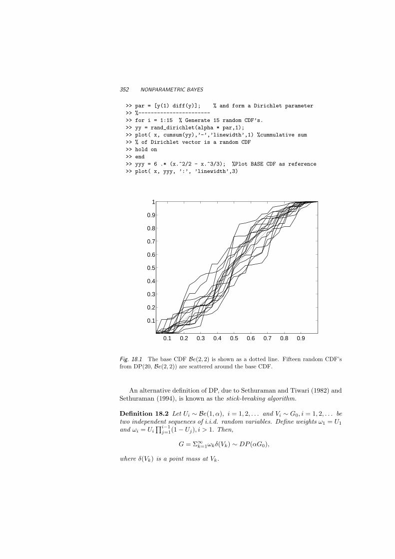
352 NONPARAMETRIC BAYES
>> par = [y(1) diff(y)]; % and form a Dirichlet parameter
>> %-----------------------
>> for i = 1:15 % Generate 15 random CDF’s.
>> yy = rand_dirichlet(alpha * par,1);
>> plot( x, cumsum(yy),’-’,’linewidth’,1) %cummulative sum
>> % of Dirichlet vector is a random CDF
>> hold on
>> end
>> yyy = 6 .* (x.^2/2 - x.^3/3); %Plot BASE CDF as reference
>> plot( x, yyy, ’:’, ’linewidth’,3)
0.1 0.2 0.3 0.4 0.5 0.6 0.7 0.8 0.9
0.1
0.2
0.3
0.4
0.5
0.6
0.7
0.8
0.9
1
Fig. 18.1 The base CDF Be(2, 2) is shown as a dotted line. Fifteen random CDF’sfrom DP(20, Be(2, 2)) are scattered around the base CDF.
An alternative definition of DP, due to Sethuraman and Tiwari (1982) andSethuraman (1994), is known as the stick-breaking algorithm.
Definition 18.2 Let Ui ∼ Be(1, α), i = 1, 2, . . . and Vi ∼ G0, i = 1, 2, . . . betwo independent sequences of i.i.d. random variables. Define weights ω1 = U1
and ωi = Ui
∏i−1j=1(1− Uj), i > 1. Then,
G = Σ∞k=1ωkδ(Vk) ∼ DP (αG0),
where δ(Vk) is a point mass at Vk.

DIRICHLET PROCESSES 353
The distribution G is discrete, as a countable mixture of point masses,and from this definition one can see that with probability 1 only discretedistributions fall in the support of DP. The name stick-breaking comes fromthe fact that Σωi = 1 with probability 1, that is, the unity is broken oninfinitely many random weights. The Definition 18.2 suggests another way togenerate approximately from a given DP.
Let GK = ΣKk=1ωkδ(Vk) where the weights ω1, . . . , ωK−1 are as in Defini-
tion 18.2 and the last weight ωK is modified as 1− ω1 − · · · − ωK−1, so thatthe sum of K weights is 1. In practical applications, K is selected so that(1− (α/(1 + α))K) is small.
18.1.1 Updating Dirichlet Process Priors
The critical step in any Bayesian inference is the transition from the prior tothe posterior, that is, updating a prior when data are available. If Y1, Y2, . . . , Yn
is a random sample from G, and G has Dirichlet prior DP (αG0), the posterioris remains Dirichlet, G|Y1, . . . , Yn ∼ DP (α∗G∗0), with α∗ = α + n, and
G∗0(t) =α
α + nG0(t) +
n
α + n
(1n
Σni=1I(Yi ≤ t ≤ ∞)
). (18.2)
Notice that the DP prior and the EDF constitute a conjugate pair because theposterior is also a DP. The posterior estimate of distribution is E(G|Y1, . . . , Yn) =G∗0(t) which is, as we saw in several examples with conjugate priors, a weightedaverage of the “prior mean” and the maximum likelihood estimator (the EDF).
Example 18.2 In the spirit of classical nonparametrics, the problem of esti-mating the CDF at a fixed value x, has a simple nonparametric Bayes solution.Suppose the sample X1, . . . , Xn ∼ F is observed and that one is interested inestimating F (x). Suppose the F (x) is assigned a Dirichlet process prior witha center F0 and a small precision parameter α. The posterior distribution forF (x) is Be(αF0(x) + `x, α(1−F0(x)) + n− `x) where `x is the number of ob-servations in the sample smaller than or equal to x. As α → 0, the posteriortends to a Be(`x, n−`x). This limiting posterior is often called noninformative.By inspecting the Be(`x, n − `x) distribution, or generating from it, one canfind a posterior probability region for the CDF at any value x. Note that theposterior expectation of F (x) is equal to the classical estimator `x/n, whichmakes sense because the prior is noninformative.
Example 18.3 The underground train at Hartsfield-Jackson airport arrivesat its starting station every four minutes. The number of people Y enteringa single car of the train is random variable with a Poisson distribution,
Y |λ ∼ P(λ).

354 NONPARAMETRIC BAYES
1
0.6
0.65
0.7
0.75
0.8
0.85
0.9
0.95
Va
lue
s
Fig. 18.2 For a sample n = 15 Beta(2,2) observations a boxplot of “noninformative”posterior realizations of P (X ≤ 1) is shown. Exact value F (1) for Beta(2,2) is shownas dotted line.
A sample of size N = 20 for Y is obtained below.
9 7 7 8 8 11 8 7 5 713 5 7 14 4 6 18 9 8 10
The prior on λ is any discrete distribution supported on integers [1, 17],
λ|P ∼ Discr ((1, 2, . . . , 17), P = (p1, p2, . . . , p17)) ,
where Σi pi = 1. The hyperprior on probabilities P is Dirichlet,
P ∼ Dir(αG0(1), αG0(2), . . . , αG0(17)).
We can assume that the prior on λ is a Dirichlet process with
G0 = [1, 1, 1, 2, 2, 3, 3, 4, 4, 5, 6, 5, 4, 3, 2, 1, 1]/48
and α = 48. We are interested in posterior inference on the rate parameter λ.
model
for (i in 1:N)
y[i] ~ dpois(lambda)

DIRICHLET PROCESSES 355
lambda ~ dcat(P[])
P[1:bins] ~ ddirch(alphaG0[])
#data
list(bins=17, alphaG0=c(1,1,1,2,2,3,3,4,4,5,6,5,4,3,2,1,1),
y=c(9,7,7,8,8,11,8,7,5,7,13,5,7,14,4,6,18,9,8,10), N=20
)
#inits
list(lambda=12,
P=c(0,0,0,0,0,0,0,0,0,0,0,1,0,0,0,0,0))
)
The summary posterior statistics were found directly from within Win-BUGS:
node mean sd MC error 2.5% median 97.5%
lambda 8.634 0.6687 0.003232 8 9 10
P[1] 0.02034 0.01982 8.556E-5 5.413E-4 0.01445 0.07282P[2] 0.02038 0.01995 78.219E-5 5.374E-4 0.01423 0.07391P[3] 0.02046 0.02004 8.752E-5 5.245E-4 0.01434 0.07456P[4] 0.04075 0.028 1.179E-4 0.004988 0.03454 0.1113P[5] 0.04103 0.028 1.237E-4 0.005249 0.03507 0.1107P[6] 0.06142 0.03419 1.575E-4 0.01316 0.05536 0.143P[7] 0.06171 0.03406 1.586E-4 0.01313 0.05573 0.1427P[8] 0.09012 0.04161 1.981E-4 0.02637 0.08438 0.1859P[9] 0.09134 0.04163 1.956E-4 0.02676 0.08578 0.1866P[10] 0.1035 0.04329 1.85E-4 0.03516 0.09774 0.2022P[11] 0.1226 0.04663 2.278E-4 0.04698 0.1175 0.2276P[12] 0.1019 0.04284 1.811E-4 0.03496 0.09649 0.1994P[13] 0.08173 0.03874 1.71E-4 0.02326 0.07608 0.1718P[14] 0.06118 0.03396 1.585E-4 0.01288 0.05512 0.1426P[15] 0.04085 0.02795 1.336E-4 0.005309 0.03477 0.1106P[16] 0.02032 0.01996 9.549E-5 5.317E-4 0.01419 0.07444P[17] 0.02044 0.01986 8.487E-5 5.475E-4 0.01445 0.07347
The main parameter of interest is the arrival rate, λ. The posterior meanof λ is 8.634. The median is 9 passengers every four minutes. Either numbercould be justified as an estimate of the passenger arrival rate per four minuteinterval. WinBUGS provides an easy way to save the simulated parametervalues, in order, to a text file. This then enables the data to be easily importedinto another environment, such as R or MATLAB, for data analysis andgraphing. In this example, MATLAB was used to provide the histograms forλ and p10. The histograms in Figure 18.3 illustrate that λ is pretty muchconfined to the five integers 7, 8, 9, 10, and 11, with the mode 9.

356 NONPARAMETRIC BAYES
6 7 8 9 10 110
0.2
0.4
0.6
0.8
1
1.2
1.4
1.6
1.8
2x 10
4
0 0.05 0.1 0.15 0.2 0.25 0.3 0.350
500
1000
1500
(a) (b)
Fig. 18.3 Histograms of 40,000 samples from the posterior for λ and P [10].
18.1.2 Generalizing Dirichlet Processes
Some popular NP Bayesian models employ a mixture of Dirichlet processes.The motivation for such models is their extraordinary modeling flexibility.Let X1, X2, . . . , Xn be the observations modeled as
Xi|θi ∼ Bin(ni, θi),θi|F ∼ F, i = 1, . . . , n (18.3)
F ∼ Dir(α).
If α assigns mass to every open interval on [0, 1] then the support of thedistributions on F is the class of all distributions on [0, 1]. This model allowsfor pooling information across the samples. For example, observation Xi willhave an effect on the posterior distribution of θj , j 6= i, via the hierarchicalstage of the model involving the common Dirichlet process.
The model (18.3) is used extensively in the applications of Bayesian non-parametrics. For example, Berry and Christensen (1979) use the model forthe quality of welding material submitted to a naval shipyard, implying aninterest in posterior distributions of θi. Liu (1996) uses the model for re-sults of flicks of thumbtacks and focusses on distribution of θn+1|X1, . . . , Xn.McEarchern, Clyde, and Liu (1999) discuss estimation of the posterior pre-dictive Xn+1|X1, . . . , Xn, and some other posterior functionals.
The DP is the most popular nonparametric Bayes model in the literature(for a recent review, see MacEachern and Mueller, 2000). However, limitingthe prior to discrete distributions may not be appropriate for some applica-

BAYESIAN CATEGORICAL MODELS 357
tions. A simple extension to remove the constraint of discrete measures is touse a convoluted DP:
X|F ∼ F
F (x) =∫
f(x|θ)dG(θ),
G ∼ DP (αG0).
This model is called Dirichlet Process Mixture (DPM), because the mix-ing is done by the DP. Posterior inference for DMP models is based onMCMC posterior simulation. Most approaches proceed by introducing la-tent variables θ as Xi|θi ∼ f(x|θi),θi|G ∼ G and G ∼ DP (αG0). EfficientMCMC simulation for general MDP models is discussed, among others, inEscobar (1994), Escobar and West (1995), Bush and MacEachern (1996)and MacEachern and Mueller (1998). Using a Gaussian kernel, f(x|µ, Σ) ∝exp(x − µ)′)Σ(x − µ)/2, and mixing with respect to θ = (µ, Σ), a densityestimate resembling traditional kernel density estimation is obtained. Suchapproaches have been studied in Lo (1984) and Escobar and West (1995).
A related generalization of Dirichlet Processes is the Mixture of DirichletProcesses (MDP). The MDP is defined as a DP with a center CDF whichdepends on random θ,
F ∼ DP (αGθ)θ ∼ π(θ).
Antoniak (1974) explored theoretical properties of MDP’s and obtained pos-terior distribution for θ.
18.2 BAYESIAN CONTINGENCY TABLES AND CATEGORICAL
MODELS
In contingency tables, the cell counts Nij can be modeled as realizationsfrom a count distribution, such as Multinomial Mn(n, pij) or Poisson P(λij).The hypothesis of interest is independence of row and column factors, H0 :pij = aibj , where ai and bj are marginal probabilities of levels of two factorssatisfying Σiai = Σjbj = 1.
The expected cell count for the multinomial distribution is ENij = npij .Under H0, this equals naibj , so by taking the logarithm on both sides, oneobtains
logENij = log n + log ai + log bj
= const + αi + βj ,

358 NONPARAMETRIC BAYES
for some parameters αi and βj . This shows that testing the model for addi-tivity in parameters α and β is equivalent to testing the original independencehypothesis H0. For the Poisson counts, the situation is analogous; one useslog λij = const + αi + βj .
Example 18.4 Activities of Dolphin Groups Revisited. We revisit theDolphin’s Activity example from p. 162. Groups of dolphins were observedoff the coast of Iceland and the table providing group counts is given below.The counts are listed according to the time of the day and the main activityof the dolphin group. The hypothesis of interest is independence of the typeof activity from the time of the day.
Travelling Feeding Socializing
Morning 6 28 38Noon 6 4 5
Afternoon 14 0 9Evening 13 56 10
The WinBUGS program implementing the additive model is quite simple.We assume the cell counts are assumed distributed Poisson and the logarithmof intensity (expectation) is represented in an additive manner. The modelparts (intercept, αi, and βj) are assigned normal priors with mean zero andprecision parameter xi. The precision parameter is given a gamma prior withmean 1 and variance 10. In addition to the model parameters, the WinBUGSprogram will calculate the deviance and chi-square statistics that measuregoodness of fit for this model.
model
for (i in 1:nrow)
for (j in 1:ncol)
groups[i,j] ~ dpois(lambda[i,j])
log(lambda[i,j]) <- c + alpha[i] + beta[j]
#
c ~ dnorm(0, xi)
for (i in 1:nrow) alpha[i] ~ dnorm(0, xi)
for (j in 1:ncol) beta[j] ~ dnorm(0, xi)
xi ~ dgamma(0.01, 0.01)
#
for (i in 1:nrow)
for (j in 1:ncol)
devG[i,j] <- groups[i,j] * log((groups[i,j]+0.5)/
(lambda[i,j]+0.5))-(groups[i,j]-lambda[i,j]);
devX[i,j] <- (groups[i,j]-lambda[i,j])
*(groups[i,j]-lambda[i,j])/lambda[i,j];
G2 <- 2 * sum( devG[,] );
X2 <- sum( devX[,] )

BAYESIAN CATEGORICAL MODELS 359
The data are imported as
list(nrow=4, ncol=3,
groups = structure(
.Data = c( 6, 28, 38, 6, 4, 5,
14, 0, 9, 13, 56, 10), .Dim=c(4,3)) ) )
and initial parameters are
list(xi=0.1, c = 0, alpha=c(0,0,0,0), beta=c(0,0,0) )
The following output gives Bayes estimators of the parameters, and mea-sures of fit. This additive model conforms poorly to the observations; underthe hypothesis of independence, the test statistic is χ2 with 3 × 4 − 6 =6 degrees of freedom, and the observed value X2 = 77.73 has a p-value(1-chi2cdf(77.73, 6)) that is essentially zero.
node mean sd MC error 2.5% median 97.5%
c 1.514 0.7393 0.03152 −0.02262 1.536 2.961alpha[1] 1.028 0.5658 0.0215 −0.07829 1.025 2.185alpha[2] −0.5182 0.5894 0.02072 −1.695 −0.5166 0.6532alpha[3] −0.1105 0.5793 0.02108 −1.259 −0.1113 1.068alpha[4] 1.121 0.5656 0.02158 0.02059 1.117 2.277beta[1] 0.1314 0.6478 0.02492 −1.134 0.1101 1.507beta[2] 0.9439 0.6427 0.02516 −0.3026 0.9201 2.308beta[3] 0.5924 0.6451 0.02512 −0.6616 0.5687 1.951c 1.514 0.7393 0.03152 −0.02262 1.536 2.961G2 77.8 3.452 0.01548 73.07 77.16 86.2X2 77.73 9.871 0.03737 64.32 75.85 102.2
Example 18.5 Cæsarean Section Infections Revisited. We now con-sider the Bayesian solution to the Cæsarean section birth problem from p.236. The model for probability of infection in a birth by Cæsarean sectionwas given in terms of the logit link as,
logP (infection)
P (no infection)= β0 + β1 noplan + β2 riskfac + β3 antibio.
The WinBUGS program provided below implements the model in which thenumber of infections is Bin(n, p) with p connected to covariates noplan riskfacand antibio via the logit link. Priors on coefficients in the linear predictorare set to be a vague Gaussian (small precision parameter).
model
for(i in 1:N)
inf[i] ~ dbin(p[i],total[i])
logit(p[i]) <- beta0 + beta1*noplan[i] +

360 NONPARAMETRIC BAYES
beta2*riskfac[i] + beta3*antibio[i]
beta0 ~dnorm(0, 0.00001)
beta1 ~dnorm(0, 0.00001)
beta2 ~dnorm(0, 0.00001)
beta3 ~dnorm(0, 0.00001)
#DATA
list( inf=c(1, 11, 0, 0, 28, 23, 8, 0),
total = c(18, 98, 2, 0, 58, 26, 40, 9),
noplan = c(0,1,0,1,0,1,0,1),
riskfac = c(1,1, 0, 0, 1,1, 0, 0),
antibio =c(1,1,1,1,0,0,0,0), N=8)
#INITS
list(beta0 =0, beta1=0,
beta2=0, beta3=0)
The Bayes estimates of the parameters β0−β3 are given in the WinBUGSoutput below.
node mean sd MC error 2.5% median 97.5%
beta0 −1.962 0.4283 0.004451 −2.861 −1.941 −1.183beta1 1.115 0.4323 0.003004 0.29 1.106 1.988beta2 2.101 0.4691 0.004843 1.225 2.084 3.066beta3 −3.339 0.4896 0.003262 −4.338 −3.324 −2.418
Note that Bayes estimators are close to the estimators obtained in the frequen-tist solution in Chapter 12: (β0, β1, β2, β3) = (−1.89, 1.07, 2.03, −3.25) andthat in addition to the posterior means, posterior medians and 95% crediblesets for the parameters are provided. WinBUGS can provide various posteriorlocation and precision measures. From the table, the 95% credible set for β0
is [−2.861,−1.183].
18.3 BAYESIAN INFERENCE IN INFINITELY DIMENSIONAL
NONPARAMETRIC PROBLEMS
Earlier in the book we argued that many statistical procedures classified asnonparametric are, in fact, infinitely parametric. Examples include waveletregression, orthogonal series density estimators and nonparametric MLEs(Chapter 10). In order to estimate such functions, we rely on shrinkage,tapering or truncation of coefficient estimators in a potentially infinite ex-pansion class. (Chencov’s orthogonal series density estimators, Fourier andwavelet shrinkage, and related.) The benefits of shrinkage estimation in statis-

INFINITELY DIMENSIONAL PROBLEMS 361
tics were first explored in the mid-1950’s by C. Stein. In the 1970’s and 1980’s,many statisticians were active in research on statistical properties of classicaland Bayesian shrinkage estimators.
Bayesian methods have become popular in shrinkage estimation becauseBayes rules are, in general, “shrinkers”. Most Bayes rules shrink large coef-ficients slightly, whereas small ones are more heavily shrunk. Furthermore,interest for Bayesian methods is boosted by the possibility of incorporatingprior information about the function to model wavelet coefficients in a realisticway.
Wavelet transformations W are applied to noisy measurements yi = fi +εi, i = 1, . . . , n, or, in vector notation, y = f + ε. The linearity of W impliesthat the transformed vector d = W (y) is the sum of the transformed signalθ = W (f) and the transformed noise η = W (ε). Furthermore, the orthog-onality of W implies that εi, i.i.d. normal N (0, σ2) components of the noisevector ε, are transformed into components of η with the same distribution.
Bayesian methods are applied in the wavelet domain, that is, after thewavelet transformation has been applied and the model di ∼ N (θi, σ
2), i =1, . . . , n, has been obtained. We can model coefficient-by-coefficient becausewavelets decorrelate and di’s are approximately independent.
Therefore we concentrate just on a single typical wavelet coefficient andone model: d = θ + ε. Bayesian methods are applied to estimate the loca-tion parameter θ. As θ’s correspond to the function to be estimated, back-transforming an estimated vector θ will give the estimator of the function.
18.3.1 BAMS Wavelet Shrinkage
BAMS (stands for Bayesian Adaptive Multiscale Shrinkage) is a simple effi-cient shrinkage in which the shrinkage rule is a Bayes rule for properly selectedprior and hyperparameters of the prior. Starting with [d|θ, σ2] ∼ N (θ, σ2) andthe prior σ2 ∼ E(µ), µ > 0, with density f(σ2|µ) = µe−µσ2
, we obtain themarginal likelihood
d|θ ∼ DE(θ,
√2µ
), with density f(d|θ) =
12
√2µe−
√2µ|d−θ|.
If the prior on θ is a mixture of a point mass δ0 at zero, and a double-exponential distribution,
θ|ε ∼ εδ0 + (1− ε)DE(0, τ), (18.4)
then the posterior mean of θ (from Bayes rule) is:
δ∗(d) =(1− ε) m(d) δ(d)
(1− ε) m(d) + ε f(d|0), (18.5)

362 NONPARAMETRIC BAYES
where
m(d) =1τ e−τ |d| − 1√
2µe−√
2µ|d|
2/τ2 − 1/µ, (18.6)
and
δ(d) =(1/τ2 − 1/(2µ))de−τ |d|/τ + (e−
√2µ|d| − e−τ |d|)/(µτ2)
(1/τ2 − 1/(2µ))(e−τ |d|/τ − e−√
2µ|d|/√
2µ). (18.7)
-4 -2 2 4
-4
-2
2
4
Fig. 18.4 Bayes rule (18.7) and comparable hard and soft thresholding rules.
As evident from Figure 18.4, the Bayes rule (18.5) falls between comparablehard- and soft-thresholding rules. To apply the shrinkage in (18.5) on a specificproblem, the hyperparameters µ, τ , and ε have to be specified. A defaultchoice for the parameters is suggested in Vidakovic and Ruggeri (2001); seealso Antoniadis, Bigot, and Sapatinas (2001) for a comparative study of manyshrinkage rules, including BAMS. Their analysis is accompanied by MATLABroutines and can be found at
http://www-lmc.imag.fr/SMS/software/GaussianWaveDen/.
Figure 18.5(a) shows a noisy doppler function of size n = 1024, wherethe signal-to-noise ratio (defined as a ratio of variances of signal and noise) is7. Panel (b) in the same figure shows the smoothed function by BAMS. Thegraphs are based on default values for the hyperparameters.
Example 18.6 Bayesian Wavelet Shrinkage in WinBUGS. Because ofthe decorrelating property of wavelet transforms, the wavelet coefficients aremodeled independently. A selected coefficient d is assumed to be normal

INFINITELY DIMENSIONAL PROBLEMS 363
0 0.2 0.4 0.6 0.8 1−15
−10
−5
0
5
10
15
0 0.2 0.4 0.6 0.8 1−15
−10
−5
0
5
10
15
(a) (b)
Fig. 18.5 (a) A noisy doppler signal [SNR=7, n=1024, noise variance σ2 = 1]. (b)Signal reconstructed by BAMS.
d ∼ N (θ, ξ) where θ is the coefficient corresponding to the underlying signalin data and ξ is the precision, reciprocal of variance. The signal componentθ is modeled as a mixture of two double-exponential distributions with zeromean and different precisions, because WinBUGS will not allow a point massprior. The precision of one part of the mixture is large (so the variance issmall) indicating coefficients that could be ignored as negligible. The cor-responding precision of the second part is small (so the variance is large)indicating important coefficients of possibly large magnitude. The densitiesin the prior mixture are taken in proportion p : (1 − p) where p is Bernoulli.For all other parameters and hyperparameters, appropriate prior distributionsare adopted.
We are interested in the posterior means for θ. Here is the WinBUGSimplementation of the described model acting on some imaginary waveletcoefficients ranging from -50 to 50, as an illustration. Figure 18.6 shows theBayes rule. Note a desirable shape close to that of the thresholding rules.
model
for (j in 1:N)
DD[j] ~ dnorm(theta[j], tau);
theta[j] <- p[j] * mu1[j] + (1-p[j]) * mu2[j];
mu1[j] ~ ddexp(0, tau1);
mu2[j] ~ ddexp(0, tau2);
p[j] ~ dbern(r);
r ~ dbeta(1,10);
tau ~ dgamma(0.5, 0.5);

364 NONPARAMETRIC BAYES
tau1 ~ dgamma(0.005, 0.5);
tau2 ~dgamma(0.5, 0.005);
#data
list( DD=c(-50, -10, -5,-4,-3,-2,-1,-0.5, -0.1, 0,
0.1, 0.5, 1, 2,3,4,5, 10, 50), N=19);
#inits
list(tau=1, tau1=0.1, tau2=10);
−50 0 50−50
−40
−30
−20
−10
0
10
20
30
40
50
Fig. 18.6 Approximation of Bayes shrinkage rule calculated by WinBUGS.
18.4 EXERCISES
18.1. Show that in the DP Definition 18.2, E(ΣTi=1ωi) = 1− [α/(1− α)]T .
18.2. Let µ =∫∞−∞ ydG(y) and let G be a random CDF with Dirichlet process
prior DP (αG0). Let y be a sample of size n from G. Using (18.2), showthat
E(µ|y) =α
α + nEµ +
n
α + ny.
In other words, show that the expected posterior mean is a weightedaverage of the expected prior mean and the sample mean.
18.3. Redo Exercise 9.13, where the results for 148 survey responses are broken

EXERCISES 365
down by program choice and by race. Test the fit of the properly setadditive Bayesian model. Use WinBUGS for model analysis.
18.4. Show that m(d) and δ(d) from (18.6) and (18.7) are marginal distribu-tions and the Bayes rule for the model is
d|θ ∼ DE(θ,
√2µ
), θ ∼ DE(0, τ),
where µ and τ are the hyperparameters.
18.5. This is an open-ended question. Select a data set with noise presentin it (a noisy signal), transform the data to the wavelet domain, applyshrinkage on wavelet coefficients by the Bayes procedure described be-low, and back-transform the shrunk coefficients to the domain of originaldata.
(i) Prove that for [d|θ] ∼ N (θ, 1), [θ|τ2] ∼ N (0, τ2), and τ2 ∼ (τ2)−3/4,the posterior is unimodal at 0 if 0 < d2 < 2 and bimodal otherwise withthe second mode
δ(d) =
(1− 1−
√1− 2/d2
2
)d.
(ii) Generalize to [d|θ] ∼ N (θ, σ2), σ2 known, and apply the larger modeshrinkage. Is this shrinkage of the thresholding type?
(iii) Use the approximation (1−u)α ∼ (1−αu) for u small to argue thatthe largest mode shrinkage is close to a James-Stein-type rule δ∗(d) =(1− 1
2d2
)+
d, where (f)+ = max0, f.18.6. Chipman, Kolaczyk, and McCulloch (1997) propose the following model
for Bayesian wavelet shrinkage (ABWS) which we give in a simplifiedform,
d|θ ∼ N (θ, σ2).
The prior on θ is defined as a mixture of two normals with a hyperprioron the mixing proportion,
θ|γ ∼ γN (0, (cτ)2) + (1− γ)N (0, τ2),γ ∼ Bin(1, p).
Variance σ2 is considered known, and c À 1.
i) Show that the Bayes rule (posterior expectation) for θ has the explicitform of
δ(d) =[P (γ = 1|d)
(cτ)2
σ2 + (cτ)2+ P (γ = 0|d)
τ2
σ2 + τ2
]d,

366 NONPARAMETRIC BAYES
where
P (γ = 1|d) =pπ(d|γ = 1)
pπ(d|γ = 1) + (1− p)π(d|γ = 0)
and π(d|γ = 1) and π(d|γ = 0) are densities of N (0, σ2 + (cτ)2) andN (0, σ2 + τ2) distributions, respectively, evaluated at d.
(ii) Plot the Bayes rule from (i) for selected values of parameters andhyperparameters (σ2, τ2, γ, c) so that the shape of the rule is reminiscentof thresholding.
REFERENCES
Antoniadis, A., Bigot, J., and Sapatinas, T. (2001), “Wavelet Estimators inNonparametric Regression: A Comparative Simulation Study,” Journalof Statistical Software, 6, 1-83.
Antoniak, C. E. (1974), “Mixtures of Dirichlet Processes with Applications toBayesian Nonparametric Problems,” Annals of Statistics, 2, 1152-1174.
Berry, D. A., and Christensen, R. (1979), “ Empirical Bayes Estimation ofa Binomial Parameter Via Mixtures of Dirichlet Processes,” Annals ofStatistics, 7, 558-568.
Bush, C. A., and MacEachern S. N. (1996), “A Semi-Parametric BayesianModel for Randomized Block Designs,” Biometrika, 83, 275-286.
Chipman, H. A., Kolaczyk, E. D., and McCulloch, R. E. (1997), “AdaptiveBayesian Wavelet Shrinkage,” Journal of American Statistical Associa-tion, 92, 1413-1421.
Escobar, M. D. (1994), “Estimating Normal Means with a Dirichlet ProcessPrior,” Journal of American Statistical Association, 89, 268-277.
Escobar, M. D., and West, M. (1995), “Bayesian Density Estimation andInference Using Mixtures, Journal of American Statistical Association,90, 577-588.
Fabius, J. (1964), “Asymptotic Behavior of Bayes’ Estimates,” Annals ofMathematical Statistics, 35, 846-856.
Ferguson, T. S. (1973), “A Bayesian Analysis of Some Nonparametric Prob-lems,” Annals of Statistics, 1, 209-230.
(1974), “Prior Distributions on Spaces of Probability Measures,”Annals of Statistics, 2, 615-629.
Freedman, D. A. (1963), “On the Asymptotic Behavior of Bayes’ Estimatesin the Discrete Case,” Annals of Mathematical Statistics, 34, 1386-1403.
Liu, J. S. (1996), “ Nonparametric Hierarchical Bayes via Sequential Imputa-

REFERENCES 367
tions,” Annals of Statistics, 24, 911-930.Lo, A. Y. (1984), “On a Class of Bayesian Nonparametric Estimates, I. Den-
sity Estimates,” Annals of Statistics, 12, 351-357.MacEachern, S. N., and Mueller, P. (1998), “Estimating Mixture of Dirichlet
Process Models, Journal of Computational and Graphical Statistics, 7,223-238.
(2000), “Efficient MCMC Schemes for Robust Model Extensions Us-ing Encompassing Dirichlet Process Mixture Models,” in Robust BayesianAnalysis, Eds. F. Ruggeri and D. Rios-Insua, New York: Springer Ver-lag.
MacEachern, S. N., Clyde, M., and Liu, J. S. (1999), “Sequential Impor-tance Sampling for Nonparametric Bayes Models: The Next Genera-tion,”Canadian Journal of Statistics, 27, 251-267.
Mueller, P., and Quintana, F. A. (2004), “Nonparametric Bayesian Data Anal-ysis,” Statistical Science, 19, 95-110.
Sethuraman, J., and Tiwari, R. C. (1982), “Convergence of Dirichlet Measuresand the Interpretation of their Parameter,” in Statistical Decision Theoryand Related Topics III, eds. S. Gupta and J. O. Berger, New York:Springer Verlag, 2, pp. 305-315.
Sethuraman, J. (1994), “A Constructive Definition of Dirichlet Priors,” Sta-tistica Sinica, 4, 639-650.
Vidakovic, B., and Ruggeri, F. (2001), “BAMS Method: Theory and Simula-tions.” Sankhya, Ser. B, 63, 234-249.


Appendix A: MATLAB
The combination of some data and an aching desire for an answer doesnot ensure that a reasonable answer can be extracted from a given bodyof data.
J. W. Tukey (1915–2000)
A.1 USING MATLAB
MATLAB is a interactive environment that allows the user to perform compu-tational tasks and create graphical output. The user types in expressions andcommands in a Command Window where numerical results of the commandsare displayed with the user input. Graphical output will be produced in anew (graphics) window that can usually be printed or stored.
When MATLAB is launched, several windows are available to the user asyou can see in Fig. A.7. Their uses are listed below:
• Command Window: Typing commands and expressions – this is themain interactive window in the user interface
• Launch Pad Window: Allows user to run demos
• Workspace Window: List of variables entered or created during ses-sion
369

370 Appendix A: MATLAB
Fig. A.7 Interactive environment of MATLAB.
• Command History Window: List of recent commands used
• Array Editor Window: Allows user to manipulate arrays variablesusing spreadsheet
• Current Directory Window: To specify directory where MATLABwill search for or store files
MATLAB is a high-level technical computing language for algorithm de-velopment, data visualization, data analysis, and numeric computation. Somehighlight features of MATLAB can be summarized as
• High-level language for technical computing, which are easy to learn
• Development environment for managing code, files, and data
• Mathematical functions for linear algebra, statistics, Fourier analysis,filtering, optimization, and numerical integration
• 2-D and 3-D graphics functions for visualizing data
• Tools for building custom graphical user interfaces
• Functions to communicate with other statistical software, such as R,WinBUGS

USING MATLAB 371
To get started, you can type doc in the command window. This will bringyou to an HTML help window and you can search keyword or browse topicstherein.
>> doc
Fig. A.8 Help window of MATLAB.
If you know the function name, but do not know how to use it, it is oftenuseful to type “help function name” in command window. For example, ifyou want to know how to use function randg or find out what randg does.
>> help randg
RANDG Gamma random numbers (unit scale).
Note: To generate gamma random numbers with specified shape and
scale parameters, you should call GAMRND.
R = RANDG returns a scalar random value chosen from a gamma
distribution with unit scale and shape.
R = RANDG(A) returns a matrix of random values chosen from gamma
distributions with unit scale. R is the same size as A, and RANDG
generates each element of R using a shape parameter equal to the
corresponding element of A.
....

372 Appendix A: MATLAB
A.1.1 Toolboxes
Serving as extensions to the basic MATLAB programming environment, tool-boxes are available for specific research interests. Toolboxes available include
Communications Toolbox
Control System Toolbox
DSP Blockset
Extended Symbolic Math Toolbox
Financial Toolbox
Frequency Domain System Identification
Fuzzy Logic Toolbox
Higher-Order Spectral Analysis Toolbox
Image Processing Toolbox
LMI Control Toolbox
Mapping Toolbox
Model Predictive Control Toolbox
Mu-Analysis and Synthesis Toolbox
NAG Foundation Blockset
Neural Network Toolbox
Optimization Toolbox
Partial Differential Equation Toolbox
QFT Control Design Toolbox
Robust Control Toolbox
Signal Processing Toolbox
Spline Toolbox
Statistics Toolbox
System Identification Toolbox
Wavelet Toolbox
For the most part we use functions in the base MATLAB product, but wherenecessary we also use functions from the Statistics Toolbox. There are numer-ous procedures from other toolboxes that can be helpful in nonparametric dataanalysis (e.g., Neural Network Toolbox, Wavelet Toolbox) but we restrict rou-tine applications to basic and fundamental computational algorithms to avoidmaking the book depend on any pre-written software code.
A.2 MATRIX OPERATIONS
MATLAB was originally written to provide easy interaction with matrix soft-ware developed by the NASA1-sponsored LINPACK and EISPACK projects.Today, MATLAB engines incorporate the LAPACK and BLAS libraries, em-bedding the state of the art in software for matrix computation. Instead of
1National Aeronautics and Space Administration.
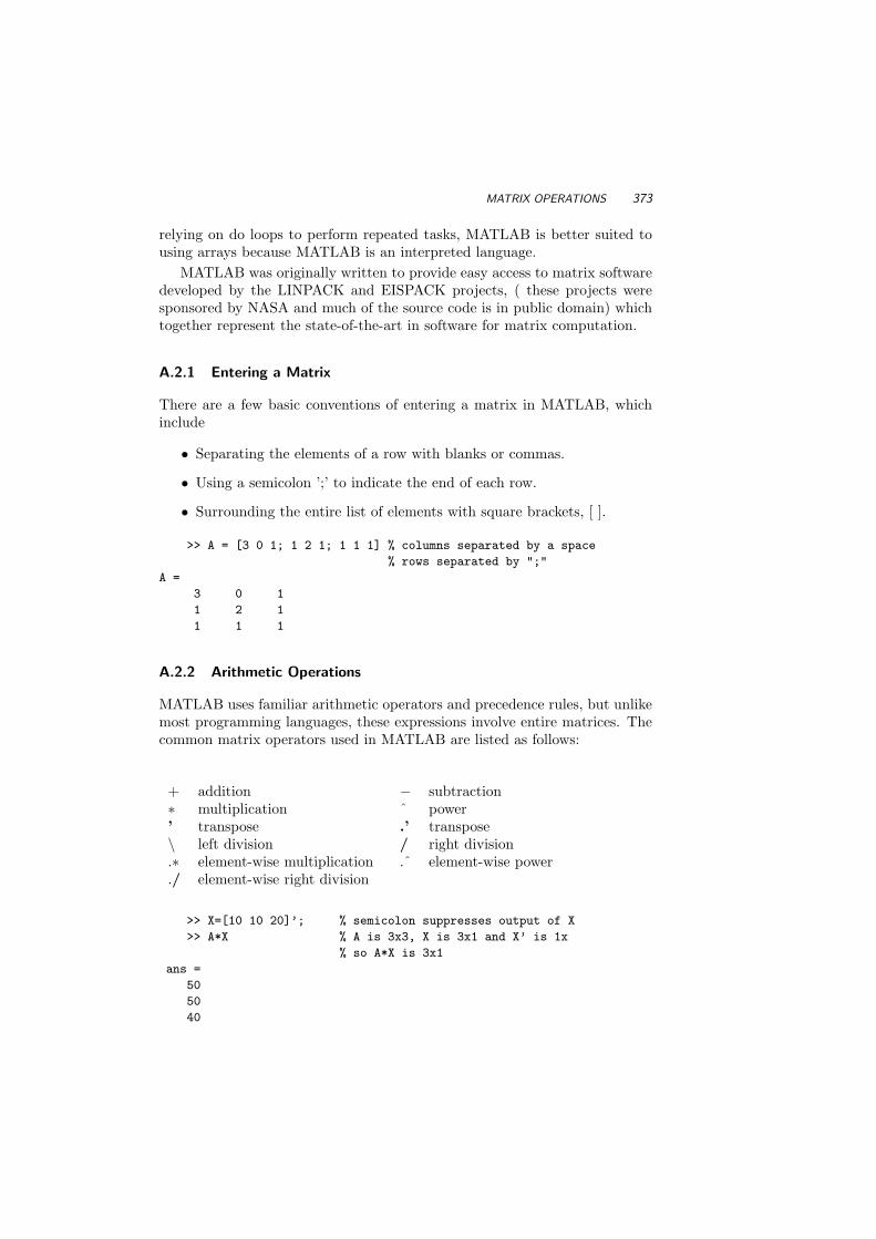
MATRIX OPERATIONS 373
relying on do loops to perform repeated tasks, MATLAB is better suited tousing arrays because MATLAB is an interpreted language.
MATLAB was originally written to provide easy access to matrix softwaredeveloped by the LINPACK and EISPACK projects, ( these projects weresponsored by NASA and much of the source code is in public domain) whichtogether represent the state-of-the-art in software for matrix computation.
A.2.1 Entering a Matrix
There are a few basic conventions of entering a matrix in MATLAB, whichinclude
• Separating the elements of a row with blanks or commas.
• Using a semicolon ’;’ to indicate the end of each row.
• Surrounding the entire list of elements with square brackets, [ ].
>> A = [3 0 1; 1 2 1; 1 1 1] % columns separated by a space
% rows separated by ";"
A =
3 0 1
1 2 1
1 1 1
A.2.2 Arithmetic Operations
MATLAB uses familiar arithmetic operators and precedence rules, but unlikemost programming languages, these expressions involve entire matrices. Thecommon matrix operators used in MATLAB are listed as follows:
+ addition − subtraction∗ multiplication ˆ power’ transpose .’ transpose\ left division / right division.∗ element-wise multiplication .ˆ element-wise power./ element-wise right division
>> X=[10 10 20]’; % semicolon suppresses output of X
>> A*X % A is 3x3, X is 3x1 and X’ is 1x
% so A*X is 3x1
ans =
50
50
40

374 Appendix A: MATLAB
>> y=A\X % y is the solution of Ay=X
y =
-10.0000
-10.0000
40.0000
>> A.*A % ".*" multiplies corresponding elements of
% matching matrices; this is equivalent to A.^2
ans =
9 0 1
1 4 1
1 1 1
A.2.3 Logical Operations
The relational operators in MATLAB are
< less than > greater than<= less-than-or-equal == equal>= greater-than-or-equal ∼= not equal& (logical) and | (logical) or∼ (logical) not
When relational operators are applied to scalars, 0 represents false and 1represents true.
A.2.4 Matrix Functions
These extra matrix functions are helpful in creating and manipulating arrays:
eye identity matrix ones matrix of oneszeros matrix of zeros diag diagonal matrixrand matrix of random U(0,1) inv matrix inversedet matrix determinant rank rank of matrixfind indices of nonzero entries norm normalized matrix
A.3 CREATING FUNCTIONS IN MATLAB
Along with the extensive collection of existing MATLAB functions, you cancreate your own problem-specific function using input variables and generating

IMPORTING AND EXPORTING DATA 375
array or graphical output. Once you look at a simple example, you can easilysee how a function is constructed. For example, here is a way to compute thePDF of a triangular distribution, centered at zero with the support [−c, c]:
function y = tripdf(x,c)
y1 = max(0,c-abs(x)) / c^2;
y = y1
The function starts with the function y = function name(input) wherey is just a dummy variable assigned as function output at the end of thefunction. Local variables (such as y1) can be defined and combined withinput variables (x,c) and the output can be scalar or matrix form. Once thefunction is named, it will override any previous function with the same name(so try not to call your function “sort”, “inv” or any other known MATLABfunction you might want to use later).
The function can be typed and saved as an m-file (i.e., tripdf.m) becausethat is how MATLAB recognizes an external file with executable code. Al-ternatively, you can type the entire function (line by line) directly into theprogram, but it won’t be automatically saved after you finish. Then you can“call” the new function as
>> v = tripdf(0:4,3)
v = [0.3333 0.2222 0.1111 0 0]
>> tripdf(-1,2) <= 0.5 % =1 if statement is true
ans =
1
It also possible to define a function as a variable. For example, if youwant to define a truncated (and unnormalized) normal PDF, use the followingcommand
>> tnormpdf = @(x, mu, sig, left, right) ...
normpdf(x,mu,sig).*(x>left & x <right);
>> tnormpdf(-3:3,0,1,-2,2)
ans =
0 0 0.2420 0.3989 0.2420 0 0
The tnormpdf function does not integrate to 1. To normalize it, one can di-vide the result by (normcdf(right,mu,sigma) - normcdf(left,mu,sigma)).
A.4 IMPORTING AND EXPORTING DATA
As a first step of data analysis, we may need to import data from externalsources. The most common types of files used in the MATLAB statistical

376 Appendix A: MATLAB
computing are MATLAB data files, Text files, and Spreadsheet files. TheMATLAB data file has the extension name *.mat. Here is an example ofimporting such data to MATLAB workspace.
A.4.1 MAT Files
You can use the command whos to look what variables are in the data file.
>> whos -file dataexample
Name Size Bytes Class
Sigma 2x2 32 double array
ans 1x1 8 double array
mu 1x2 16 double array
xx 500x2 8000 double array
Grand total is 1007 elements using 8056 bytes
Then you can use the command load to load all variables in this data file.
>> clear % clear variables in the workspace
>> load dataexample
>> whos % check what variables are in the workspace
Name Size
Bytes Class
Sigma 2x2 32 double array
ans 1x1 8 double array
mu 1x2 16 double array
xx 500x2 8000 double array
Grand total is 1007 elements using 8056 bytes
In some cases, you may only want to load some variables in the MAT file tothe workspace. Here is how you can do it.
>> clear
>> varlist = ’Sigma’,’mu’; % Created a list of variables
>> load(’dataexample.mat’,varlist:)
>> clear varlist % remove varlist from workspace
>> whos % see what is in the workspace
Name Size Bytes Class

IMPORTING AND EXPORTING DATA 377
Sigma 2x2 32 double array
mu 1x2 16 double array
Grand total is 6 elements using 48 bytes
Another way of creating variables of interest is to use an index.
>> clear
>> vars = whos(’-file’, ’dataexample.mat’);
>> load(’dataexample.mat’,vars([1,3]).name)
If you do not want to use full variable names, but want to use some patternsin these names, the load command can be used with a ’-regexp’ option. Thefollowing command will load the same variable as the previous one.
>> load(’dataexample.mat’, ’-regexp’, ’^S|^m’);
Text files usually have the extension name *.txt, *.dat, *.csv, and so forth.
A.4.2 Text Files
If the data in the text file are organized as a matrix, you can still use load toimport the data into the workspace.
>> load mytextdata.dat
>> mytextdata
mytextdata =
-0.3097 0.2950 -0.1681 -1.4250
-1.5219 -0.3927 -0.6873 0.4615
0.8265 0.5759 -0.9907 1.0915
-0.6130 -1.1414 -0.0498 -1.0443
0.9597 0.0611 0.7193 -2.8428
1.9730 0.0123 -0.2831 0.9968
You can also assign the loading data to be stored in a new variable.
>> x = load(’mytextdata.dat’);
The command load will not work if the text file is not organized in matrixform. For example, if you have a text file mydata.txt
>> type mydata.txt
var1 var2 var3 var4 name
-0.3097 0.2950 -0.1681 -1.4250 Olive
-1.5219 -0.3927 -0.6873 0.4615 Richard

378 Appendix A: MATLAB
0.8265 0.5759 -0.9907 1.0915 Dwayne
-0.6130 -1.1414 -0.0498 -1.0443 Edwin
0.9597 0.0611 0.7193 -2.8428 Sheryl
1.9730 0.0123 -0.2831 0.9968 Frank
You should use a new function txtread to import variables to workspace.
>> [var1,var2,var3,var4,str] = ...
textread(’mydata.txt’,’%f%f%f%f%s’,’headerlines’,1 );
Alternatively, you can use textscan to finish the import.
>> fid = fopen(’mydata.txt’);
>> C = textscan(fid, ’%f%f%f%f%s’,’headerLines’,1);
>> fclose(fid);
>> [C1:4] % var1 - var4
ans =
-0.3097 0.2950 -0.1681 -1.4250
-1.5219 -0.3927 -0.6873 0.4615
0.8265 0.5759 -0.9907 1.0915
-0.6130 -1.1414 -0.0498 -1.0443
0.9597 0.0611 0.7193 -2.8428
1.9730 0.0123 -0.2831 0.9968
>> C5 % name
ans =
’Olive’
’Richard’
’Dwayne’
’Edwin’
’Sheryl’
’Frank’
Comma-separated values files are useful when exchanging data. Given thefile data.csv that contains the comma-separated values
>> type data.csv
02, 04, 06, 08, 10, 12
03, 06, 09, 12, 15, 18
05, 10, 15, 20, 25, 30
07, 14, 21, 28, 35, 42
11, 22, 33, 44, 55, 66
You can use csvread to read the entire file into workspace
>> csvread(’data.csv’)

IMPORTING AND EXPORTING DATA 379
ans =
2 4 6 8 10 12
3 6 9 12 15 18
5 10 15 20 25 30
7 14 21 28 35 42
11 22 33 44 55 66
A.4.3 Spreadsheet Files
Data from a spreadsheet can be imported into the workspace using the func-tion xlsread.
>> [NUMERIC,TXT,RAW]=xlsread(’data.xls’);
>> NUMERIC
NUMERIC =
1.0000 0.3000 NaN
2.0000 0.4500 NaN
3.0000 0.3000 12.0000
4.0000 0.3500 5.0000
5.0000 0.3500 5.0000
6.0000 0.3500 10.0000
7.0000 0.3500 13.0000
8.0000 0.3500 5.0000
9.0000 0.3500 23.0000
>> TXT
TXT =
’Date ’ ’var1 ’ ’var2’ ’var3’ ’name’
’1/1/2001’ ’’ ’’ ’’ ’Frank’
’1/2/2001’ ’’ ’’ ’’ ’’
’1/3/2001’ ’’ ’’ ’’ ’Sheryl’
’1/4/2001’ ’’ ’’ ’’ ’’
’1/5/2001’ ’’ ’’ ’’ ’Richard’
’1/6/2001’ ’’ ’’ ’’ ’Olive’
’1/7/2001’ ’’ ’’ ’’ ’Dwayne’
’1/8/2001’ ’’ ’’ ’’ ’Edwin’
’1/9/2001’ ’’ ’’ ’’ ’Stan’
>> RAW
RAW =
’Date ’ ’var1 ’ ’var2’ ’var3’ ’name’
’1/1/2001’ [ 1] [0.3000] [ NaN] ’Frank’
’1/2/2001’ [ 2] [0.4500] [ NaN] [ NaN]

380 Appendix A: MATLAB
’1/3/2001’ [ 3] [0.3000] [ 12] ’Sheryl’
’1/4/2001’ [ 4] [0.3500] [ 5] [ NaN]
’1/5/2001’ [ 5] [0.3500] [ 5] ’Richard’
’1/6/2001’ [ 6] [0.3500] [ 10] ’Olive’
’1/7/2001’ [ 7] [0.3500] [ 13] ’Dwayne’
’1/8/2001’ [ 8] [0.3500] [ 5] ’Edwin’
’1/9/2001’ [ 9] [0.3500] [ 23] ’Stan’
It is also possible to specify the sheet name of xls file as the source of thedata.
>> NUMERIC = xlsread(’data.xls’,’rnd’); % read data from
% a sheet named as rnd
From an xls file, you can get data from a specified region in a named sheet:
>> NUMERIC = xlsread(’data.xls’,’data’,’b2:c10’);
The following command also allows you do interactive region selection:
>> NUMERIC = xlsread(’data.xls’,-1);
The simplest way to save the variables from a workspace to a permanentfile in the format of a MAT file is to use the command save. If you have asingle matrix to save, save filename varname -ascii will save export theresult to text file. You can also save numeric array or cell array in an Excelworkbook using xlswrite.
A.5 DATA VISUALIZATION
A.5.1 Scatter Plot
A scatterplot is a useful summary of a set of bivariate data (two variables),usually drawn before working out a linear correlation coefficient or fitting aregression line. It gives a good visual picture of the relationship betweenthe two variables, and aids the interpretation of the correlation coefficient orregression model.
In MATLAB, a simple way of make a plot matrix is to use the commandplot. Fig. A.9 gives the result of the following MATLAB commands:
>> x = rand(1000,1);
>> y = .5*x + 5*x.^2 + .3*randn(1000,1);
>> plot(x,y,’.’)
However, this is is not enough if you are dealing with more than two variables.In this case, the function plotmatrix should used in stead (Fig.A.10).

DATA VISUALIZATION 381
0 0.2 0.4 0.6 0.8 1−1
0
1
2
3
4
5
6
Fig. A.9 Scatterplot of (x, y) for x = rand(1000,1) and y = .5*x + 5*x.2 +
.3*randn(1000,1).
>> x = randn(50,3);
>> y = x*[-1 2 1;2 0 1;1 -2 3;]’;
>> plotmatrix(y)
In classification problems, it is also useful to look at scatter plot matrix withgrouping variable (Fig.A.11).
>> load carsmall;
>> X = [MPG,Acceleration,Displacement,Weight,Horsepower];
>> varNames = ’MPG’ ’Acceleration’ ’Displacement’ ...
’Weight’ ’Horsepower’;
>> gplotmatrix(X,[],Cylinders,’bgrcm’,[],[],’on’,’hist’,varNames);
>> set(gcf,’color’,’white’)
A.5.2 Box Plot
Box plot is an excellent tool for conveying location and variation informationin data sets, particularly for detecting and illustrating location and variationchanges between different groups of data. Here is an example of how MATLABmakes a boxplot (Fig. A.12).
>> load carsmall
>> boxplot(MPG, Origin, ’grouporder’, ...
’France’ ’Germany’ ’Italy’ ’Japan’ ’Sweden’ ’USA’)
>> set(gcf,’color’,’white’)

382 Appendix A: MATLAB
−10 0 10−5 0 5−10 0 10
−10
−5
0
5
10
−5
0
5
−10
−5
0
5
10
Fig. A.10 Simulated data visualized by plotmatrix.
100 200Horsepower
200030004000Weight
200 400Displacement
10 20Acceleration
20 40
100
200
MPG
Hors
epow
er 2000
3000
4000
Weig
ht
200
400
Dis
pla
cem
ent 10
20
Accele
ration
20
40
MP
G
468
Fig. A.11 Scatterplot matrix for Car Data.

DATA VISUALIZATION 383
France Germany Italy Japan Sweden USA
10
15
20
25
30
35
40
45
Val
ues
Fig. A.12 Boxplot for Car Data.
A.5.3 Histogram and Density Plot
A histogram of univariate data can be plotted using hist (Fig.A.13),
>> hist(randn(100,1))
while a three-dimensional histogram of bivariate data is plotted usinghist3, (Fig.A.14),
>> mu = [1 -1]; Sigma = [.9 .4; .4 .3];
>> r = mvnrnd(mu, Sigma, 500);
>> hist3(r)
If you like a smoother density plot, you may turn to a kernel density ordistribution estimate implemented in ksdensity (Fig.A.15). Also, in recentversions of MATLAB you have the option of not asking for outputs from theksdensity, and the function plots the results directly.
>> [y,x] = ksdensity(randn(100,1));
>> plot(x,y)
A.5.4 Plotting Function List
Here is a complete list of statistical plotting functions available in MATLAB

384 Appendix A: MATLAB
−2.5 −2 −1.5 −1 −0.5 0 0.5 1 1.5 20
2
4
6
8
10
12
14
16
18
20
Fig. A.13 Histogram for simulated random normal data.
Fig. A.14 Spatial histogram for simulated two-dimensional random normal data.

DATA VISUALIZATION 385
−5 −3 −1 1 3 40
0.1
0.2
0.3
0.4
Fig. A.15 Kernel density estimator for simulated random normal data.
andrewsplot - Andrews plot for multivariate data.
bar - Bar graph.
biplot - Biplot of variable/factor coefficients and scores.
boxplot - Boxplots of a data matrix (one per column).
cdfplot - Plot of empirical cumulative distribution function.
contour - Contour plot.
ecdf - Empirical CDF (Kaplan-Meier estimate).
ecdfhist - Histogram calculated from empirical CDF.
fplot - Plots scalar function $f(x)$ at values of $x$.
fsurfht - Interactive contour plot of a function.
gline - Point, drag and click line drawing on figures.
glyphplot - Plot stars or Chernoff faces for multivariate data.
gname - Interactive point labeling in x-y plots.
gplotmatrix - Matrix of scatter plots grouped by a common variable.
gscatter - Scatter plot of two variables grouped by a third.
hist - Histogram (in MATLAB toolbox).
hist3 - Three-dimensional histogram of bivariate data.
ksdensity - Kernel smoothing density estimation.
lsline - Add least-square fit line to scatter plot.
normplot - Normal probability plot.
parallelcoords - Parallel coordinates plot for multivariate data.
probplot - Probability plot.
qqplot - Quantile-Quantile plot.
refcurve - Reference polynomial curve.
refline - Reference line.
stairs - Stair-step of y with jumps at points x.
surfht - Interactive contour plot of a data grid.

386 Appendix A: MATLAB
wblplot - Weibull probability plot.
A.6 STATISTICS
For your convenience, let’s look at a list of functions that can be used tocompute summary statistics from data.
corr - Linear or rank correlation coefficient.
corrcoef - Correlation coefficient with confidence intervals.
cov - Covariance.
crosstab - Cross tabulation.
geomean - Geometric mean.
grpstats - Summary statistics by group.
harmmean - Harmonic mean.
iqr - Interquartile range.
kurtosis - Kurtosis.
mad - Median Absolute Deviation.
mean - Sample average (in MATLAB toolbox).
median - 50th percentile of a sample.
moment - Moments of a sample.
nancov - Covariance matrix ignoring NaNs.
nanmax - Maximum ignoring NaNs.
nanmean - Mean ignoring NaNs.
nanmedian - Median ignoring NaNs.
nanmin - Minimum ignoring NaNs.
nanstd - Standard deviation ignoring NaNs.
nansum - Sum ignoring NaNs.
nanvar - Variance ignoring NaNs.
partialcorr - Linear or rank partial correlation coefficient.
prctile - Percentiles.
quantile - Quantiles.
range - Range.
skewness - Skewness.
std - Standard deviation (in MATLAB toolbox).
tabulate - Frequency table.
trimmean - Trimmed mean.
var - Variance

STATISTICS 387
A.6.1 Distributions
Distribution CDF PDF Inverse CDF RNG
Beta betacdf betapdf betainv betarnd
Binomial binocdf binopdf binoinv binornd
Chi square chi2cdf chi2pdf chi2inv chi2rnd
Exponential expcdf exppdf expinv exprnd
Extreme value evcdf evpdf evinv evrnd
F fcdf fpdf finv frnd
Gamma gamcdf gampdf gaminv gamrnd
Geometric geocdf geopdf geoinv geornd
Hypergeometric hygecdf hygepdf hygeinv hygernd
Lognormal logncdf lognpdf logninv lognrnd
Multivariate normal mvncdf mvnpdf mvninv mvnrnd
Negative binomial nbincdf nbinpdf nbininv nbinrnd
Normal (Gaussian) normcdf normpdf norminv normrnd
Poisson poisscdf poisspdf poissinv poissrnd
Rayleigh raylcdf raylpdf raylinv raylrnd
t tcdf tpdf tinv trnd
Discrete uniform unidcdf unidpdf unidinv unidrnd
Uniform distribution unifcdf unifpdf unifinv unifrnd
Weibull wblcdf wblpdf wblinv wblrnd
A.6.2 Distribution Fitting
betafit - Beta parameter estimation.
binofit - Binomial parameter estimation.
evfit - Extreme value parameter estimation.
expfit - Exponential parameter estimation.
gamfit - Gamma parameter estimation.
gevfit - Generalized extreme value parameter estimation.
gpfit - Generalized Pareto parameter estimation.
lognfit - Lognormal parameter estimation.
mle - Maximum likelihood estimation (MLE).
mlecov - Asymptotic covariance matrix of MLE.
lognfit - Negative binomial parameter estimation.
normfit - Normal parameter estimation.
poissfit - Poisson parameter estimation.
raylfit - Rayleigh parameter estimation.
unifit - Uniform parameter estimation.
wblfit - Weibull parameter estimation.
In addition to the command line function listed above, there is also a GUIto used for distribution fitting. You can use the command dfittool to invokethis tool (Fig.A.16).

388 Appendix A: MATLAB
>> dfittool
Fig. A.16 GUI for dfittool.
A.6.3 Nonparametric Procedures
kstest - Kolmogorov-Smirnov two-sample test.
kstest2 - Kolmogorov-Smirnov one or two-sample test
mtest - Cramer Von Mises test for normality
dagosptest - D’Agostino-Pearson’s test for normality
runs_test - Runs test
sign_test1 - Two-sample sign test.
kruskal_wallis - Kruskal-Wallis rank test.
friedman - Friedman randomized block design test
kendall - Computes Kendall’s tau correlation statistic
spear - Spearman correlation coefficient.
wmw - Wilcoxon-Mann-Whitney two-sample test.
tablerxc - test of independence for $r$x$c$ table.
mantel_haenszel- Mantel-Haenszel statistic for $2$x$2$ tables.
The listed nonparametric functions that are not distributed with MATLABor its Statistics Toolbox can be downloaded from the book home page.

STATISTICS 389
A.6.4 Regression Models
A.6.4.1 Ordinary Least Squares (OLS) The most straightforward way of im-plementing OLS is based on normal equations.
>> x = rand(20,1);
>> y = 2 + 3*x + randn(size(x));
>> X = [ones(length(x),1),x];
>> b = inv(X’*X)*X’*y % normal equation
b =
1.8778
3.4689
A better solution uses backslash because it is more numerically stable thaninv.
>> b2 = X\y
b2 =
1.8778
3.4689
The pseudo inverse function pinv is also an option. It too is numericallystable, but it will yield subtly different results when your matrix is singularor nearly so. Is pinv better? There are arguments for both backslash andpinv. The difference really lies in what happens on singular or nearly singularmatrixes. pinv will not work on sparse problems, and because pinv relies onthe singular value decomposition, it may be slower for large problems.
>> b3 = pinv(X)*y
b3 =
1.8778
3.4689
Large-scale problems where X is sparse may sometimes benefit from asparse iterative solution. lsqr is an iterative solver.
>> b4 = lsqr(X,y,1.e-13,10)
lsqr converged at iteration 2 to a solution with relative residual 0.33

390 Appendix A: MATLAB
b4 =
1.8778
3.4689
There is another option, lscov. lscov is designed to handle problemswhere the data covariance matrix is known. It can also solve a weightedregression problem.
>> b5 = lscov(X,y)
b5 =
1.8778
3.4689
Directly related to the backslash solution is one based on the QR factor-ization. If our over-determined system of equations to solve is Xb = y , thena quick look at the normal equations,
b = (X ′X)−1X ′y
combined with the qr factorization of X,
X = QR
yieldsb = (R′Q′QR)−1R′Q′y.
Of course, we know that Q is an orthogonal matrix, so Q’Q is an identitymatrix.
b = (R′R)−1R′Q′y
If R is non-singular, then (R′R)−1 = R−1R′−1, so we can further reduce to
b = R−1Q′y
This solution is also useful for computing confidence intervals on the param-eters.
>> [Q,R] = qr(X,0);
>> b6 = R\(Q’*y)
b6 =
1.8778
3.4689
A.6.4.2 Weighted Least Squares (WLS) Weighted Least Squares (WLS) isspecial case of Generalized Least Squares (GLS). It should be applied when

STATISTICS 391
there is heteroscedasticity in the regression, i.e. the variance of the error termis not a constant across observations. The optimal weights should be inverselyproportional to the error variances.
>> x = (1:10)’;
>> wgts = 1./rand(size(x));
>> y = 2 + 3*x + wgts.*randn(size(x));
>> X = [ones(length(x),1),x];
>> b7 = lscov(M,y,wgts)
b7 =
-89.6867
27.9335
Another alternative way of doing WLS is to transform the independentand dependent variables so that we apply OLS to the transformed data.
>> yw = y.*sqrt(wgts);
>> Xw = X.*repmat(sqrt(wgts),1,size(M,2));
>> b8 = Xw\yw
coef8 =
-89.6867
27.9335
A.6.4.3 Iterative Reweighted Least Squares (IRLS) IRLS can be used for mul-tiple purposes. One is to get robust estimates by reducing the effect of out-liers. Another is to fit a generalized linear model, as described in SectionA.6.6. MATLAB provides a function robustfit which performs iterativereweighted least squares estimation which yield robust coefficient estimates.
>> x = (1:10)’;
>> y = 10 - 2*x + randn(10,1); y(10) = 0;
>> brob = robustfit(x,y)
brob =
10.5208
-2.0902
A.6.4.4 Nonlinear Least Squares MATLAB provides a function nlinfit whichperforms nonlinear least squares estimation.
>> mymodel = @(beta, x) (beta(1)*x(:,2) - x(:,3)/beta(5)) ./ ...
(1+beta(2)*x(:,1)+beta(3)*x(:,2)+beta(4)*x(:,3));
>> load reaction;

392 Appendix A: MATLAB
>> beta = nlinfit(reactants,rate,mymodel,ones(5,1))
beta =
1.2526
0.0628
0.0400
0.1124
1.1914
A.6.4.5 Other Regression Functions
coxphfit - Cox proportional hazards regression.
nlintool - Graphical tool for prediction in nonlinear models.
nlpredci - Confidence intervals for prediction in nonlinear models.
nlparci - Confidence intervals for parameters in nonlinear models.
polyconf - Polynomial evaluation and with confidence intervals.
polyfit - Least-squares polynomial fitting.
polyval - Predicted values for polynomial functions.
rcoplot - Residuals case order plot.
regress - Multivariate linear regression, also return the
R-square statistic, the F statistic and p value for
the full model, and an estimate of the error variance.
regstats - Regression diagnostics for linear regression.
ridge - Ridge regression.
rstool - Multidimensional response surface visualization (RSM).
stepwise - Interactive tool for stepwise regression.
stepwisefit - Non-interactive stepwise regression.
A.6.5 ANOVA
The following function set can be used to perform ANOVA in a parametricor nonparametric fashion.
anova1 - One-way analysis of variance.
anova2 - Two-way analysis of variance.
anovan - n-way analysis of variance.
aoctool - Interactive tool for analysis of covariance.
friedman - Friedman’s test (nonparametric two-way anova).
kruskalwallis - Kruskal-Wallis test (nonparametric one-way anova).
A.6.6 Generalized Linear Models
MATLAB provides the glmfit and glmval functions to fit generalized linearmodels. These models include Poisson regression, gamma regression, andbinary probit or logistic regression. The functions allow you to specify a linkfunction that relates the distribution parameters to the predictors. It is also

STATISTICS 393
possible to fit a weighted generalized linear model. Fig. A.17 is a result ofthe following MATLAB commands:
>> x = [2100 2300 2500 2700 2900 3100 3300 3500 3700 3900 4100 4300]’;
>> n = [48 42 31 34 31 21 23 23 21 16 17 21]’;
>> y = [1 2 0 3 8 8 14 17 19 15 17 21]’;
>> b = glmfit(x, [y n], ’binomial’, ’link’, ’probit’);
>> yfit = glmval(b, x, ’probit’, ’size’, n);
>> plot(x, y./n, ’o’, x, yfit./n, ’-’)
2000 2500 3000 3500 4000 45000
0.1
0.2
0.3
0.4
0.5
0.6
0.7
0.8
0.9
1
Fig. A.17 Probit regression example.
A.6.7 Hypothesis Testing
MATLAB also provide a set of functions to perform some important statisticaltests. These tests include tests on location or dispersion. For example, ttestand ttest2 can be used to do a t test.
Hypothesis Tests.
ansaribradley - Ansari-Bradley two-sample test for equal dispersions.
dwtest - Durbin-Watson test for autocorrelation in regression.
ranksum - Wilcoxon rank sum test (independent samples).
runstest - Runs test for randomness.
signrank - Wilcoxon sign rank test (paired samples).
signtest - Sign test (paired samples).

394 Appendix A: MATLAB
ztest - Z test.
ttest - One sample t test.
ttest2 - Two sample t test.
vartest - One-sample test of variance.
vartest2 - Two-sample F test for equal variances.
vartestn - Test for equal variances across multiple groups.
Distribution tests, sometimes called goodness of fit tests, are also included.For example, kstest and kstest2 are functions to perform a Kolmogorov-Smirnov test.
Distribution Testing.
chi2gof - Chi-square goodness-of-fit test.
jbtest - Jarque-Bera test of normality.
kstest - Kolmogorov-Smirnov test for one sample.
kstest2 - Kolmogorov-Smirnov test for two samples.
lillietest - Lilliefors test of normality.
A.6.8 Statistical Learning
The following function provide tools to develop data mining/machine learningprograms.
Factor Models
factoran - Factor analysis.
pcacov - Principal components from covariance matrix.
pcares - Residuals from principal components.
princomp - Principal components analysis from raw data.
rotatefactors - Rotation of FA or PCA loadings.
Decision Tree Techniques.
treedisp - Display decision tree.
treefit - Fit data using a classification or regression tree.
treeprune - Prune decision tree or create optimal pruning sequence.
treetest - Estimate error for decision tree.
treeval - Compute fitted values using decision tree.
Discrimination Models
classify - Discriminant analysis with ’linear’, ’quadratic’,
’diagLinear’, ’diagQuadratic’, or ’mahalanobis’ discriminant function
A.6.9 Bootstrapping
In MATLAB, boot and bootci are used to obtain boostrap estimates. Theformer is used to draw bootstrapped samples from data and compute thebootstrapped statistics based on these samples. The latter computes theimproved bootstrap confidence intervals, including the BCa interval.

STATISTICS 395
>> load lawdata gpa lsat
>> se = std(bootstrp(1000,@corr,gpa,lsat))
>> bca = bootci(1000,@corr,gpa,lsat)
se =
0.1322
bca =
0.3042
0.9407


Appendix B: WinBUGS
Beware: MCMC sampling can be dangerous! (Disclaimer from WinBUGS User Man-
ual)
bugs is freely available software for constructing Bayesian statistical modelsand evaluating them using MCMC methodology.
BUGS and WinBUGS are distributed freely and are the result of manyyears of development by a team of statisticians and programmers at the Med-ical research Council Biostatistics Research Unit in Cambridge (BUGS andWinBUGS), and from recently by a team at University of Helsinki (Open-BUGS) see the project pages: http://www.mrc-bsu.cam.ac.uk/bugs/ andhttp://mathstat.helsinki.fi/openbugs/.
Models are represented by a flexible language, and there is also a graphicalfeature, doodlebugs, that allows users to specify their models as directedgraphs. For complex models the doodlebugs can be very useful. As of May2007, the latest version of WinBUGS is 1.4.1 and OpenBUGS 3.0.
397

398 Appendix B: WinBUGS
B.1 USING WINBUGS
We start the introduction to WinBUGS with a simple regression example.Consider the model
yi|µi, τ ∼ N (µi, τ), i = 1, . . . , n
µi = α + β(xi − x),α ∼ N (0, 10−4)β ∼ N (0, 10−4)τ ∼ Gamma(0.001, 0.001).
The scale in normal distributions here is parameterized in terms of a precisionparameter τ which is the reciprocal of variance, τ = 1/σ2. Natural distribu-tions for the precision parameters are gamma and small values of the precisionreflect the flatness (noninformativeness) of the priors. The parameters α andβ are less correlated if predictors xi − x are used instead of xi. Assume that(x, y)-pairs (1, 1), (2, 3), (3, 3), (4, 3), and (5, 5) are observed.
Estimators in classical, Least Square regression of y on x− x, are given inthe following table.
Coef LSEstimate SE Coef t p
ALPHA 3.0000 0.3266 9.19 0.003
BETA 0.8000 0.2309 3.46 0.041
S = 0.730297 R-Sq = 80.0% R-Sq(adj) = 73.3%
How about Bayesian estimators? We will find the estimators by MCMCcalculations as means on the simulated posteriors. Assume that the initialvalues of parameters are α0 = 0.1, β0 = 0.6, and τ = 1. Start bugs and inputthe following code in [File > New].
# A simple regression
model
for (i in 1:N)
Y[i] ~ dnorm(mu[i],tau);
mu[i] <- alpha + beta * (x[i] - x.bar);
x.bar <- mean(x[]);
alpha ~ dnorm(0, 0.0001);
beta ~ dnorm(0, 0.0001);
tau ~ dgamma(0.001, 0.001);
sigma <- 1.0/sqrt(tau);
#-----------------------------
#these are observations
list( x=c(1,2,3,4,5), Y=c(1,3,3,3,5), N=5);
#-----------------------------
#the initial values

USING WINBUGS 399
list(alpha = 0.1, beta = 0.6, tau = 1);
Next, put the cursor at an arbitrary position within the scope of modelwhich delimited by wiggly brackets. Select the Model menu and open Spec-ification. The Specification Tool window will pop-out. If your model ishighlighted, you may check model in the specification tool window. If themodel is correct, the response on the lower bar of the bugs window shouldbe: model is syntactically correct. Next, highlight the “list” statementin the data-part of your code. In the Specification Tool window select loaddata. If the data are in correct format, you should receive response on thebottom bar of bugs window: data loaded. You will need to compile yourmodel on order to activate inits-buttons. Select compile in the SpecificationTool window. The response should be: model compiled, and the buttonsload inits and gen inits become active. Finally, highlight the “list” state-ment in the initials-part of your code and in the Specification Tool windowselect load inits. The response should be: model is initialized, and thisfinishes reading in the model. If the response is initial values loaded butthis or other chain contain uninitialized variables, click on the geninits button. The response should be: initial values generated, modelinitialized.
Now, you are ready to Burn-in some simulations and at the same timecheck that the program is working. In the Model menu, choose Update...and open Update Tool to check if your model updates.
From the Inference menu, open Samples.... A window titled SampleMonitor Tool will pop out. In the node sub-window input the names of thevariables you want to monitor. In this case, the variables are alpha, beta,and tau. If you correctly input the variable the set button becomes activeand you should set the variable. Do this for all 3 variables of interest. In fact,sigma as transformation of tau is available, as well.
Now choose alpha from the subwindow in Sample Monitor Tool. All ofthe buttons (clear, set, trace, history, density, stats, coda, quantiles,bgr diag, auto cor) are now active. Return to Update Tool and select thedesired number of simulations, say 10000, in the updates subwindow. Pressthe update button.
Return to Sample Monitor Tool and check trace for the part of MCtrace for α, history for the complete trace, density for a density estimatorof α, etc. For example, pressing stats button will produce something like thefollowing table
mean sd MCerror val2.5pc median val97.5pc start sample
alpha 3.003 0.549 0.003614 1.977 3.004 4.057 10000 20001
The mean 3.003 is the Bayes estimator (as the mean from the sample fromthe posterior for α. There are two precision outputs, sd and MCerror. The

400 Appendix B: WinBUGS
former is an estimator of the standard deviation of the posterior and can beimproved by increasing the sample size but not the number of simulations.The later one is the error of simulation and can be improved by additionalsimulations. The 95% credible set is bounded by val2.5pc and val97.5pc,which are the 0.025 and 0.975 (empirical) quantiles from the posterior. Theempirical median of the posterior is given by median. The outputs start andsample show the starting index for the simulations (after burn-in) and theavailable number of simulations.
0 1 2 3 4 5 60
0.2
0.4
0.6
0.8
1
−1 −0.5 0 0.5 1 1.5 2 2.5 30
0.2
0.4
0.6
0.8
1
1.2
1.4
1.6
(a) (b)
0 2 4 6 8 100
0.05
0.1
0.15
0.2
0.25
0.3
0.35
1 2 3 4 50
0.2
0.4
0.6
0.8
1
1.2
(c) (d)
Fig. B.18 Traces of the four parameters from simple example: (a) α, (b) β, (c) τ,and (d) σ from WinBUGS. Data are plotted in MATLAB after being exported fromWinBUGS.
For all parameters a comparative table is

BUILT-IN FUNCTIONS 401
mean sd MCerror val2.5pc median val97.5pc start sample
alpha 3.003 0.549 0.003614 1.977 3.004 4.057 10000 20001beta 0.7994 0.3768 0.002897 0.07088 0.7988 1.534 10000 20001tau 1.875 1.521 0.01574 0.1399 1.471 5.851 10000 20001
sigma 1.006 0.7153 0.009742 0.4134 0.8244 2.674 10000 20001
If you want to save the trace for α in a file and process it in MATLAB,say, select coda and the data window will open with an information windowas well. Keep the data window active and select Save As from the Filemenu. Save the αs in alphas.txt where it will be ready to be imported toMATLAB.
Kevin Murphy lead the project for communication between WinBUGS andMATLAB:
http://www.cs.ubc.ca/~murphyk/Software/MATBUGS/matbugs.html.
His suite matbugs, maintained by several researchers, communicates withWinBUGS directly from MATLAB.
B.2 BUILT-IN FUNCTIONS AND COMMON DISTRIBUTIONS IN
BUGS
This section contains two tables: one with the list of built-in functions andthe second with the list of available distributions.
The first-time WinBUGS user may be disappointed by the selection ofbuilt in functions – the set is minimal but sufficient. The full list of dis-tributions in WinBUGS can be found in Help>WinBUGS User Manualunder The BUGS language: stochastic nodes>Distributions. BUGSalso allows for construction of distributions for which are not in default list.In Table B.23 a list of important continuous and discrete distributions, withtheir BUGS syntax and parametrization, is provided. BUGS has the capa-bility to define custom distributions, both as likelihood or as a prior, via theso called zero-Poisson device.

402 Appendix B: WinBUGS
Table B.22 Built-in Functions in WinBUGS
BUGS Code function
abs(y) |y|cloglog(y) ln(− ln(1− y))cos(y) cos(y)equals(y, z) 1 if y = z; 0 otherwiseexp(y) exp(y)inprod(y, z) Σiyizi
inverse(y) y−1 for symmetric positive-definite matrix ylog(y) ln(y)logfact(y) ln(y!)loggam(y) ln(Γ(y))logit(y) ln(y/(1− y))max(y, z) y if y > z; y otherwisemean(y) n−1Σiyi, n = dim(y)min(y, z) y if y < z; z otherwisephi(y) standard normal CDF Φ(y)pow(y, z) yz
sin(y) sin(y)sqrt(y)
√y
rank(v, s) number of components of v less than or equal to vs
ranked(v, s) the sth smallest component of vround(y) nearest integer to ysd(y) standard deviation of components of ystep(y) 1 if y ≥ 0; 0 otherwisesum(y) Σiyi
trunc(y) greatest integer less than or equal to y

BUILT-IN FUNCTIONS 403D
istr
ibuti
on
BU
GS
Code
Den
sity
Ber
noulli
x∼
dbern(p)
px(1−
p)1−
x,
x=
0,1
;0≤
p≤
1B
inom
ial
x∼
dbin(p,
n)
` n x
´ px(1−
p)n−
x,
x=
0,.
..,n
;0≤
p≤
1C
ate
gori
cal
x∼
dcat(p[])
p[x
],x
=1,2
,...
,dim
(p)
Pois
son
x∼
dpois(lambda)
λx
x!
exp−
λ,
x=
0,1
,2,.
..,
λ>
0
Bet
ax∼
dbeta(a,b)
1B
(a,b
)x
a−
1(1−
x)b−
1,
0=
x≤
1,
a,b
>−1
Chi-sq
uare
x∼
dchisqr(k)
xk
/1−
1exp−
x/2
2k
/2Γ(k
/2)
,x≥
0,
k>
0
Double
Exponen
tial
x∼
ddexp(mu,
tau)
τ 2ex
p−
τ|x−
µ|,
x∈
R,
τ>
0,
µ∈
RE
xponen
tial
x∼
dexp(lambda)
λex
p−
λx,
x≥
0,
λ≥
0Fla
tx∼
dflat()
const
ant;
not
apro
per
den
sity
Gam
ma
x∼
dgamma(a,
b)
ba
xa−
1
Γ(a
)ex
p(−
bx),
x,a
,b>
0
Norm
al
x∼
dnorm(mu,
tau)
pτ/(2
π)ex
p−
τ 2(x−
µ)2,
x,µ∈
R,τ
>0
Pare
tox∼
dpar)alpha,c)
αcα
x−
(α+
1),x
>c
Stu
den
t-t
x∼
dt(mu,
tau,
k)
Γ((
k+
1)/
2)
Γ(k
/2)
qτ kπ
[1+
τ k(x−
µ)2
]−(k
+1)/
2,x∈R,
k≥
2
Uniform
x∼
dunif(a,
b)
1b−
a,
a≤
x≤
b
Wei
bull
x∼
dweib(v,
lambda)
vλx
v−
1ex
p−
λx
v,
x,v
,λ>
0,
Mult
inom
ial
x[]∼
dmulti(p[],N)
(Σix
i)!
Qi
xi!
Qip
xi
i,Σ
ix
i=
N,0
<p
i<
1,Σ
ip
i=
1
Dir
ichle
tp[]∼
ddirch(alpha[])
Γ(Σ
iα
i)
QiΓ(α
i)
Qip
αi−
1i
,0
<p
i<
1,Σ
ip
i=
1
Mult
ivari
ate
Norm
al
x[]∼
dmnorm(mu[],T[,])
(2π)−
d/2|T|1/
2ex
p−
1/2(x−
µ)′
T(x−
µ)
,x∈
Rd
Mult
ivari
ate
Stu
den
t-t
x[]∼
dmt(mu[],T[,],
k)
Γ((
k+
d)/
2)
Γ(k
/2)
|T|1
/2
kd
/2π
d/2
ˆ 1+
1 k(x−
µ)′
T(x−
µ)˜−
(k+
d)/
2,
x∈Rd
,k≥
2
Wis
hart
x[,]∼
dwish(R[,],k)
|R|k/
2|x|(k−
p−
1)/
2ex
p−
1/2T
r(R
x)
Tab
leB
.23
Bui
lt-in
dist
ribu
tion
sw
ith
BU
GS
nam
esan
dth
eir
para
met
riza
tion
s.


MATLAB Index
CDF eta, 352
KMcdfSM, 293
LMSreg, 226
WavMat.m, 270
andrewsplot, 386
anova1, 392
anova2, 392
anovan , 392
ansaribradley, 394
aoctool, 392
bar, 386
bessel, 11, 92
beta, 10
betacdf, 21, 387
betafit, 387
betainc, 10, 75, 78
betainv, 21, 77, 387
betapdf, 21, 70, 387
betarnd, 387
bincdf, 38, 177
binlow, 39
binocdf, 14, 167, 387
binofit, 387
binoinv, 387
binopdf, 14, 40, 387
binoplot, 14
binornd, 387
binup, 39
biplot, 386
bootci, 394
bootsample, 290, 304
boxplot, 381, 386
cdfplot, 386
chi2cdf, 19, 157--159, 177, 387
chi2gof, 394
chi2inv, 19, 387
chi2pdf, 19, 387
chi2rnd, 387
ciboot, 291, 293
classify, 394
clear, 376
contour, 386
conv, 272
corcoeff, 386
corr, 298, 386
corrcoef, 290
cov, 386
coxphfit, 197
crosstab, 386
csapi, 253
csvread, 378
dagosptest, 388
dfittool, 387
diff, 298

406 MATLAB INDEX
dwtest, 394
dwtr, 271
ecdf, 386
ecdfhist, 386
elm, 199
evcdf, 387
evfit, 387
evinv, 387
evpdf, 387
evrnd, 387
expcdf, 18, 387
expfit, 387
expinv, 18, 387
exppdf, 18, 387
exprnd, 18, 387
factoran, 394
factorial, 9
fcdf, 23, 387
finv, 23, 387
fliplr, 272
floor, 10
fnplt, 253
forruns, 105
fpdf, 23, 387
fplot, 329, 386
friedman, 147, 388, 392
friedman pairwise comparison, 147
frnd, 387
fsurfht, 386
gamcdf, 18, 387
gamfit, 387
gaminv, 18, 387
gamma, 10
gammainc, 10
gampdf, 18, 387
gamrnd, 387
geocdf, 16, 387
geoinv, 16, 387
geomean, 386
geopdf, 16, 387
geornd, 16, 387
gevfit, 387
gline, 386
glmfit, 236, 392
glmval, 236, 392
glyphplot, 386
gplotmatrix, 381
grpstats, 386
gscatter, 344
harmean, 386
hist, 206, 298, 383
hist3, 386
histfit, 207
hygecdf, 16, 387
hygeinv, 16, 387
hygepdf, 16, 387
hygernd, 16, 387
idwtr, 272
inv, 388
iqr, 386
jackrsp, 295
jbtest, 394
kdfft2, 213
kendall, 388
kmcdfsm, 188
kruskal wallis, 143, 388
kruskalwallis, 392
ksdensity, 211, 383
kstest, 88, 388, 394
kstest2, 88, 388, 394
kurtosis, 386
lillietest, 394
lmsreg, 224
load, 376
loc lin, 247
loess, 249
loess2, 249
logist, 328, 329
logistic, 328
logncdf, 387
lognfit, 387
logninv, 387
lognpdf, 387
lognrnd, 387
lpfit, 247
lscov, 224, 226, 388
lsline, 386
lsqr, 388
lts, 226
mad, 386
mantel haenszel, 170, 388
mean, 386
median, 386
medianregress, 226
mixture cla, 313
mle, 387
mlecov, 387
moment, 386

MATLAB INDEX 407
mtest, 92, 97, 388
mvncdf, 387
mvninv, 387
mvnpdf, 387
mvnrnd, 383, 387
nada wat, 245
nancov, 386
nanmax, 386
nanmean, 386
nanmedian, 386
nanstd, 386
nansum, 386
nanvar, 386
nbincdf, 15, 387
nbininv, 15, 387
nbinpdf, 15, 387
nbinrnd, 15, 387
nchoosek, 9
nearneighbor, 331
nlinfit, 392
nlintool, 392
nlparci, 392
nlpredci, 392
normcdf, 19, 35, 387
normfit, 387
norminv, 19, 110, 387
normpdf, 19, 387
normplot, 386
normrnd, 387
parallelcoords, 386
partialcorr, 386
pcacov, 394
pcares, 394
pinv, 388
plot, 35, 329, 341
plotedf, 35
plotmatrix, 381
pluginmu, 195
poisscdf, 15, 387
poissfit, 387
poissinv, 15, 387
poisspdf, 15, 387
poissrnd, 15, 30, 387
polyconf , 392
polyfit, 392
polyval, 392
prctile, 386
princomp, 394
problow, 104
probplot, 97, 386
probup, 104
qqgamma, 100
qqnorm, 100
qqplot, 99, 111, 386
qqweib, 98, 100
quantile, 386
rand, 331
rand irichlet, 352
randg, 371
randn, 35, 380
range, 386
rank, 118
ranksum, 394
raylcdf, 387
raylfit, 387
raylinv, 387
raylpdf, 387
raylrnd, 387
rcoplot , 392
refcurve, 386
refline, 386
regress, 392
regstats, 392
ridge , 392
robustfit , 392
rotatefactors, 394
round, 331
rstool, 392
runs test, 104, 388
runstest, 394
sign test1, 121, 388
signrank, 394
signtest, 394
size, 344
skewness, 386
softmax, 337
sort, 298
spear, 124, 388
spline, 252
squaredrankstest, 134
stairs, 386
std, 386
stepwise, 392
stepwisefit , 392
surfht, 386
survband, 193
tablerxc, 162, 388
tabulate, 386

408 MATLAB INDEX
tcdf, 20, 387
textread, 378
textscan, 378
tinv, 20, 387
tnormpdf, 375
tpdf, 20, 387
treedisp, 343
treefit, 343, 344, 394
treeprune, 343, 394
treetest, 344
treeval, 344, 394
trimmean, 291, 293, 386
tripdf, 375
trnd, 387
ttest, 394
ttest2, 394
type, 378
unidcdf, 387
unidinv, 387
unidpdf, 387
unidrnd, 387
unifcdf, 387
unifinv, 387
unifit, 387
unifpdf, 387
unifrnd, 387
var, 386
vartest, 394
vartest2, 394
vartestn, 394
wblcdf, 387
wblfit, 387
wblinv, 387
wblpdf, 387
wblrnd, 387
wbplt, 386
whos, 376
wilcoxon signed, 128
wilcoxon signed2, 127
wmw, 132, 388
xlsread, 379
xlswrite, 380
ztest, 394

Author Index
Anscombe, F. J., 47
Agresti, A., 40, 154, 327Altman, N. S., 247, 258Anderson, T. W., 90Anscombe, F. J., 47, 226Antoniadis, A., 273, 362Antoniak, C. E., 357Arvin, D. V., 125
Bai, Z., 77Baines, L., 205Baines, M. J., 258Balmukand, B., 308Bayes, T., 47, 48Bellman, R. E., 331Benford, F., 158Berger, J. O., 58Berry, D. A., 356Best, N. G., 62Bickel, P. J., 174Bigot, J., 273, 362Birnbaum, Z. W., 83Bradley, J. V., 2Breiman, L., 342Broffitt, J.D., 327Brown, J. S., 183
Buddha, 81Bush, C. A., 357
Carter, W. C., 199Casella, G., 1, 42, 62Charles, J. A., 299Chen, M.-H., 62Chen, Z., 77Chernick, M. R., 302Christensen, R., 356Cleveland, W., 247Clopper, C. J., 39Clyde, M., 356Cochran, W. G., 167Congdon, P., 62Conover, W. J., 2, 134, 148Cox, D. R., 196Cramer, H., 91Crowder, M. J., 188Crowley, J., 308Cummings, T. L., 177
D’Agostino, R. B., 96Darling, D. A., 90Darwin, C., 154Daubechies, I., 266Davenport, J. M., 146

410 AUTHOR INDEX
David, H. A., 69Davies, L., 212Davis, T. A., 6Davison, A. C., 302de Hoog, F. R., 256Delampady, M., 58Deming, W. E., 323Dempster, A. P., 307Donoho, D., 273, 276Doob, J., 12Doucet, H., 177Duda, R. O., 324Dunn, O., 327Dykstra, R. L., 227
Ebert, R., 174Efromovich, S., 211Efron, B., 286, 292Elsner, J. B., 340Epanechnickov, V. A., 210Escobar, M. D., 357Excoffier, L., 308
Fabius, J., 350Fahrmeir, L., 236Falconer, S., 121Feller, W., 12Ferguson, T. S., 350Finey, D. J., 65Fisher, R. A., 6, 41, 107, 154, 161,
163, 308, 329Folks, L. J., 107Fourier, J., 266Freedman, D. A., 350Friedman, J., 324, 336, 337, 342Friedman, M., 145Frieman, S. W., 199Fuller Jr., E. R., 199
Gasser, T, 257Gather, U., 212Gelfand, A. E., 61George, E. O., 108Gilb, T., 167Gilks, W. R., 62Good, I. J., 108Good, P. I., 302Gosset, W. S., 20, 154Graham, D., 167Green, P. J., 255
Haar, A., 266Haenszel, W., 168Hall, W. J., 193Hammel, E. A., 174Hart, P. E., 324Hastie, T., 324, 336Healy M. J. R., 307Hedges, L. V., 107Hendy, M. F., 299Hettmansperger, T.P., 1Hill, T., 158Hinkley, D. V., 302Hoeffding, W., 1Hogg, R. V., 327Hotelling, H., 115Hubble, E. P., 289Huber, P. J., 222, 223Hume, B., 153Hutchinson, M. F., 256
Ibrahim, J., 62Iman, R. L., 134, 146
Johnson, R., 166Johnson, S., 166Johnstone, I., 273, 276
Kohler, W., 257Kahm, M. J., 177Kahneman, D., 5Kaplan, E. L., 188, 294Kaufman, L., 137Kendall, M. G., 125Kiefer, J., 184Kimber, A. C., 188Kimberlain, T. B., 340Kolmogorov, A. N., 81Krishnan, T., 308Kruskal, J., 337Kruskal, W. H., 115, 142Kutner, M.A., 328Kvam, P. H., 219, 316
Laird, N. M., 307Lancaster, H. O., 108Laplace, P. S., 9Lawless, J. F., 196Lawlor E., 318Lehmann, E. L., 42, 131, 149Lehmiller, G. S., 340

AUTHOR INDEX 411
Leroy A. M., 223, 224Lindley, D. V., 65Liu, J. S., 356Liu, Z., 169Lo, A. Y., 357Luben, R.N., 136
Muller, H. G., 257MacEachern, S. N., 357Madigan, D., 65Mahalanobis, P. C., 286Mallat, S., 270Mandel, J., 124Mann, H., 115Mantel, N., 168Marks, S., 327Martz, H., 59Mattern, R., 249Matui, I., 179McCullagh, P., 231McEarchern, S. M., 356McFly, G., 205McKendrick, A. G., 307McLachlan, G. J., 308McNemar, Q., 164Meier, P., 188, 294Mencken, H. L., 1Mendel, G., 154Michelson, A., 110Miller, L. A., 162Molinari, L., 257Moore, D. H., 327Mudholkar, G. S., 108Mueller, P., 350, 356, 357Muenchow, G., 188
Nachtsheim, C. J., 328Nadaraya, E. A., 244Nair, V. J., 193Nelder, J. A., 231Neter, J., 328
O’Connell, J.W., 174Ogden, T., 266Olkin, I., 107Olshen, R., 342Owen, A. B., 199
Pabst, M., 115Pareto, V., 23
Pearson, E. S., 39, 163Pearson, K., 6, 39, 81, 154, 161, 206Pepys, S., 5Phillips, D. P., 176Piotrowski, H., 163Pitman, E. J. G., 286Playfair, W., 206Popper, K., 36Preece, M. A., 258
Quade, D., 147Quenouille, M. H., 286, 295Quinlan, J. R., 345Quinn, G. D., 199Quinn, J. B., 199Quintana, F. A., 350
Radelet, M., 172Ramberg, J. S., 327Randles, R. H., 1, 327Rao, C. R., 308Rasmussen, M. H., 162Raspe, R. E., 287Reilly, M., 318Reinsch, C. H., 255Richey, G.G., 124Rickey, B., 141Robert, C., 62Robertson, T., 227Rock, I., 137Roeder, K., 84Rosenblatt, F., 333Rousseeuw P. J., 223, 224Rubin, D. B., 296, 307Ruggeri, F., 362
Sager, T. W., 77Samaniego, F. J., 316Sapatinas, T., 273, 362Scanlon, F.L., 136Scanlon, T.J., 136Schuler, F., 249Schmidt, G., 249Schoenberg, I. J., 251Selke, T., 58Sethuraman, J., 352Shah, M.K., 177Shakespeare, W., 285Shao, Q.-M., 62Shapiro, S. S., 93

412 AUTHOR INDEX
Shen, X., 266Sigmon, K., 6Silverman, B. W., 211, 255Simonoff, J. S., 154Singleton, N., 136Sinha, B. K., 77Siskel, G., 174Slatkin, M., 308Smirnov, N. V., 81, 86Smith, A. F. M., 61Smith, R. L., 188Spaeth, R., 125Spearman, C. E., 122Speed, T., 309Spiegelhalter, D. J., 62Stephens, M. A., 90, 96Stichler, R.D., 124Stigler, S. M., 188Stokes, S. L., 77Stone, C., 342Stork, D. G., 324Stuetzle, W., 337Sweeting, T. J., 188
Thisted, R. A., 314Thomas, A., 62Tibshirani, R. J., 292, 324, 336Tingey, F., 83Tippet, L. H. C., 107Tiwari, R. C., 352Tsai, W. Y., 308Tutz, G., 236
Tversky, A., 5Twain, M., xiii
Utts, J., 108
van Gompel, R., 121Vidakovic, B., 266, 273, 362Voltaire, F. M., 6von Bortkiewicz, L., 157von Mises, R., 91
Waller, R., 59Wallis, W. A., 142Walter, G. G., 266Wasserman, L., 2Watson, G. S., 244Wedderburn, R. W. M., 231Weierstrass, K., 253Wellner, J., 193West, M., 357Westmacott M. H., 307Wilcoxon, F., 115, 127Wilk, M. B., 93Wilkinson, B., 107Wilks, S. S., 43Wilson, E. B., 40Wolfowitz, J., 1, 184Wright, S., 69Wright, T. F., 227Wu, C. F. J., 308
Young, N., 33

Subject Index
Accelerated life testing, 197Almost-sure convergence, 28Analysis of variance, 116, 141, 142Anderson-Darling test, 89Anscombe’s data sets, 226Artificial intelligence, 323
BAMS wavelet shrinkage, 361Bandwidth
choice of, 210optimal, 210
Bayesnonparametric, 349
Bayes classifier, 325Bayes decision rule, 326Bayes factor, 57Bayes formula, 11Bayesian computation, 61Bayesian statistics, 47
prediction, 59bootstrap, 296conjugate priors, 54expert opinion, 51hyperperameter, 48hypothesis testing, 56interval estimation, 55loss functions, 53
point estimation, 52
posterior distribution, 49
prior distribution, 48
prior predictive, 49
Bayesian testing, 56
of precise hypotheses, 58
Lindley paradox, 65
Benford’s law, 158
Bernoulli distribution, 14
Bessel functions, 11
Beta distribution, 20
Beta function, 10
Beta-binomial distribution, 24
Bias, 325
Binary classification trees, 338
growing, 341
impurity function, 339
cross entropy, 339
Gini, 339
misclassification, 339
pruning, 342
Binomial distribution, 4, 14, 32
confidence intervals, 39
normal approximation, 40
relation to Poisson, 15
test of hypothesis, 37

414 SUBJECT INDEX
Binomial distributionstolerance intervals, 74
Bootstrap, 285, 325Bayesian, 296bias correction, 292fallibility, 302nonparametric, 287percentile, 287
Bowman-Shenton test, 94Box kernel function, 209Brownian bridge, 197Brownian motion, 197Byzantine coins, 299
Categorical data, 153contingency tables, 159goodness of fit, 155
Cauchy distribution, 21Censoring, 185, 212
type I, 186type II, 186
Central limit theorem, 1, 29extended, 31multinomial probabilities, 170
Central moment, 13Chance variables, 12Characteristic functions, 13, 32Chi square test
rules of thumb, 156Chi-square distribution, 19, 32Chi-square test, 146, 155Classification
binary trees, 338linear models, 326nearest neighbor, 329, 331neural networks, 333supervised, 324unsupervised, 324
Classification and Regression Trees (CART),338
Cochran’s test, 167Combinations, 9Compliance monitoring, 74Concave functions, 11Concomitant, 186, 191Conditional expectation, 14Conditional probability, 11Confidence intervals, 39
binomial proportion, 39, 40
Clopper-Pearson, 39for quantiles, 73Greenwood’s formula, 193Kaplan-Meier estimator, 192likelihood ratio, 43normal distribution, 43one sided, 39pointwise, 193simultaneous band, 193two sided, 39Wald, 40
Confirmation bias, 5Conjugate priors, 54Conover test, 133, 148
assumptions, 133Consistent estimators, 29, 34Contingency tables, 159, 177
rxc tables, 161Fisher exact test, 163fixed marginals, 163McNemar test, 165
Convergence, 28almost sure, 28in distribution, 28in probability, 28
Convex functions, 11Correlation, 13Correlation coefficient
Kendall’s tau, 125Pearson, 116Spearman, 116
Covariance, 13Covariate, 195Cramer-von Mises test, 91, 97, 112Credible sets, 55Cross validation, 325
binary classification trees, 343test sample, 325, 330training sample, 325, 330
Curse of dimensionality, 331Curve fitting, 242Cæsarean birth study, 236
D’Agostino-Pearson test, 94Data
Bliss beetle data, 239California
well water level, 278Fisher’s iris data, 329

SUBJECT INDEX 415
horse-kick fatalities, 157Hubble’s data, 297interval, 4, 153Mendel’s data, 156motorcycle data, 249nominal, 4, 153ordinal, 4, 153
Data mining, 323Delta method, 29Density estimation, 184, 205
bandwidth, 207bivariate, 213kernel, 207
adaptive kernels, 210box, 209Epanechnickov, 209normal, 209triangular, 209
smoothing function, 208Designed experiments, 141Detrending data, 250Deviance, 234Dirichlet distribution, 22, 350Dirichlet process, 350, 351, 354, 356
conjugacy, 353mixture, 357mixture of, 357noninformative prior, 353
Discrete distributionsbeta-binomial, 53
Discriminant analysis, 323, 324Discrimination function
linear, 326quadratic, 326
Distributions, 12continuous, 17
beta, 20Cauchy, 21chi-square, 19, 32Dirichlet, 22, 297, 350double exponential, 21, 361exponential, 17, 32F, 23gamma, 18Gumbel, 76, 113inverse gamma, 22Laplace, 21Lorentz, 21negative-Weibull, 76
normal, 18Pareto, 23Student’s t, 20uniform, 20, 32Weibull, 59, 60
discrete, 14Bernoulli, 14beta-binomial, 24binomial, 4, 14Dirac mass, 59geometric, 16hypergeometric, 16multinomial, 16, 160, 185, 232negative binomial, 15Poisson, 15, 32truncated Poisson, 320uniform, 304
empirical, 34convergence, 36
exponential family, 25mixture, 23
EM algorithm estimation, 311normal, 32
uniform, 70Dolphins
Icelandic, 162Double exponential distribution, 21,
361
Efficiencyasymptotic relative, 3, 44, 148hypothesis testing, 44nonparametric methods, 3
EM Algorithm, 307definition, 308
Empirical density function, 184, 205Empirical distribution function, 34, 183
convergence, 36Empirical likelihood, 43, 198Empirical process, 197Epanechikov kernel, 244Epanechnickov kernel function, 209Estimation, 33
consistent, 34unbiased, 34
Expectation, 12Expected value, 12Expert opinion, 51Exponential distribution, 17, 32

416 SUBJECT INDEX
Exponential family of distributions, 25Extreme value theory, 75
F distribution, 23Failure rate, 17, 27, 195Fisher exact test, 163Formulas
counting, 10geometric series, 10Newton’s, 11Sterling’s, 10Taylor series, 11
Fox news, 153Friedman pairwise comparisons, 147Friedman test, 116Functions
Bessel, 11beta, 10characteristic, 13, 32
Poisson distribution, 31convex and concave, 11empirical distribution, 34gamma, 10incomplete beta, 10incomplete gamma, 10moment generating, 13Taylor series, 32
Gamma distribution, 18Gamma function, 10Gasser-Muller estimator, 245General tree classifiers, 345
AID, 345CART, 345CLS, 345hybrids, 345OC1, 345SE-trees, 345
Generalized linear models, 230algorithm, 232link functions, 233
GeneticsMendel’s findings, 154
Geometric distribution, 16maximum likelihood estimator, 42
Geometric series, 10Glivenko-Cantelli theorem, 36, 197Goodness of fit, 81, 156
Anderson-Darling test, 89
Bowman-Shenton test, 94chi-square, 155choosing a test, 94Cramer-von Mises test, 91, 97,
112D’Agostino-Pearson test, 94discrete data, 155Lilliefors test, 94Shapiro-Wilks test, 93two sample test, 86
Greenwood’s formula, 193Gumbel distribution, 76, 113
Heisenberg’s principle, 264Histogram, 206
bins, 206Hogmanay, 120Hubble telescope, 288Huber estimate, 222Hypergeometric distribution, 16Hypothesis testing, 36
p-values, 37Bayesian, 56binomial proportion, 37efficiency, 44for variances, 148null versus alternative, 36significanc level, 36type I error, 36type II error, 37unbiased, 37Wald test, 37
Incomplete beta function, 10Incomplete gamma function, 10Independence, 11, 12Indicator function, 34Inequalities
Cauchy-Schwartz, 13, 26Chebyshev, 26Jensen, 26Markov, 26stochastic, 26
Inter-arrival times, 176Interpolating splines, 252Interval scale data, 4, 153Inverse gamma distribution, 22Isotonic regression, 227
Jackknife, 295, 325

SUBJECT INDEX 417
Joint distributions, 12
k-out-of-n system, 78Kaplan-Meier estimator, 185, 188
confidence interval, 192Kendall’s tau, 125Kernel
beta family, 244Epanechikov, 244
Kernel estimators, 243Kolmogorov statistic, 82, 109
quantiles, 84Kolmogorov-Smirnov test, 82–84, 90Kruskal-Wallis test, 141, 143, 149, 150
pairwise comparisons, 144
L2 convergence, 28Laplace distribution, 21Law of total probability, 11Laws of large numbers (LLN), 29Least absolute residuals regression, 222Least median squares regression, 224Least squares regression, 218Least trimmed squares regression, 223Lenna image, 281Likelihood, 41
empirical, 43maximum likelihood estimation,
41Likelihood ratio, 43
confidence intervals, 43nonparametric, 198
Lilliefors test, 94Linear classification, 326Linear discrimination function, 326Linear rank statistics, 131
U -statistics, 131Links, 233
complementary log-log, 234logit, 234probit, 234
Local polynomial estimator, 246LOESS, 247Logistic regression, 327
missclassification error, 328Loss functions
cross entropy, 325in neural networks, 335zero-one, 325, 327
Machine learning, 323Mann-Whitney test, 116, 131, 141
equivalence to Wilcoxon sum ranktest, 132
relation to ROC curve, 203Mantel-Haenszel test, 167Markov chain Monte Carlo (MCMC),
61MATLAB
ANOVA, 392data visualization, 380exporting data, 375functions, 374implementation, 5importing data, 375matrix operations, 372nonparametric functions, 388regression, 389statistics functions, 386windows, 369
Maximum likelihood estimation, 41Cramer-Rao lower bound, 42delta method, 42geometric distribution, 42invariance property, 42logistic regression, 328negative binomial distribution, 42nonparametric, 184, 185, 191regularity conditions, 42
McNemar test, 165Mean square convergence, 28Mean squared error, 34, 36Median, 13
one sample test, 118two sample test, 119
Memoryless property, 16, 18Meta analysis, 106, 157, 169
averaging p-values, 108Fisher’s inverse χ2 method, 107Tippet-Wilkinson method, 107
Misclassification error, 328Moment generating functions, 13Multinomial distribution, 16, 185
central limit theorem, 170Multiple comparisons
Friedman test, 147Kruskal-Wallis test, 144test of variances, 149
Multivariate distributions

418 SUBJECT INDEX
Dirichlet, 22multinomial, 16
Nadaraya-Watson estimator, 244Natural selection, 154Nearest neighbor
classification, 329constructing, 331
Negative binomial distribution, 15maximum likelihood estimator, 42
Negative Weibull distribution, 76Neural networks, 323, 333
activation function, 334, 336back-propagation, 334, 336feed-forward, 333hidden layers, 334implementing, 336layers, 333MATLAB toolbox, 336perceptron, 333training data, 335two-layer, 334
Newton’s formula, 11Nominal scale data, 4, 153Nonparametric
definition, 1density estimation, 205estimation, 183
Nonparametric Bayes, 349Nonparametric Maximum likelihood es-
timation, 184, 185, 191Nonparametric meta analysis, 106Normal approximation
central limit theorem, 19for binomial, 40
Normal distribution, 18confidence intervals, 43conjugacy, 49kernel function, 209mixture, 32
Normal probability plot, 97
Order statistics, 69, 115asymptotic distributions, 75density function, 70distribution function, 70EM Algorithm, 315extreme value theory, 75independent, 76
joint distribution, 70maximum, 70minimum, 70, 191
Ordinal scale data, 4, 153Over-dispersion, 24, 314Overconfidence bias, 5
Parallel system, 70Parametric assumptions, 115
analysis of variance, 142criticisms, 3tests for, 81
Pareto distribution, 23Pattern recognition, 323Percentiles
sample, 72Perceptron, 333Permutation tests, 298Permutations, 9Plug-in principle, 193Poisson distribution, 15, 32
in sign test, 120relation to binomial, 15
Poisson process, 176Pool adjacent violators algorithm (PAVA),
230Posterior, 49
odds, 57Posterior predictive distribution, 49Power, 37, 38Precision parameter, 64Prior, 49
noninformative, 353odds, 57
Prior predictive distribution, 49Probability
Bayes formula, 11conditional, 11continuity theorem, 31convergence
almost sure, 28central limit theorem, 1, 29delta method, 29extended central limit theorem,
31Glivenko-Cantelli theorem, 36,
197in L2, 28in distribution, 28

SUBJECT INDEX 419
in Mean square, 28in probability, 28Laws of Large Numbers, 29Lindberg’s condition, 31Slutsky’s theorem, 29
density function, 12independence, 11joint distributions, 12law of total probability, 11mass function, 12
Probability density function, 12Probability plotting, 97
normal, 97two samples, 98
Product limit estimator, 188Projection pursuit, 337Proportional hazards model, 196
Quade test, 147Quadratic discrimination function, 326Quantile-quantile plots, 98Quantiles, 13
estimation, 194sample, 72
Racial bigotryby scientists, 155
Random variables, 12characteristic function, 13conditional expectation, 14continuous, 12correlation, 13covariance, 13discrete, 12expected value, 12independent, 12median, 13moment generating function, 13quantile, 13variance, 13
Randomized block design, 116, 145Range, 69Rank correlations, 115Rank tests, 115, 142Ranked set sampling, 76Ranks, 116, 141
in correlation, 122linear rank statistics, 118properties, 117
Receiver operating characteristic, 202Regression
change point, 66generalized linear, 230isotonic, 227least absolute residuals, 222least median squares, 224least squares, 218least trimmed squares, 223logistic, 327robust, 221Sen-Theil estimator, 221weighted least squares, 223
Reinsch algorithm, 255Relative risk, 162Resampling, 286Robust, 44, 141Robust regression, 221
breakdown point, 222leverage points, 224
ROC curve, 202are under curve, 203
Runs test, 100, 111normal approximation, 103
Sample range, 69distribution, 72tolerance intervals, 74
Semi-parametric statisticsCox model, 196inference, 195
Sen-Theil estimator, 221Series system, 70, 191Shapiro-Wilks test, 93
coefficients, 94quantiles, 94
Shrinkage, 53Clopper-Pearson Interval, 40
Sign test, 116, 118assumptions, 118paired samples, 119ties in data, 122
Signal processing, 323Significance level, 36Simpson’s paradox, 172Slutsky’s theorem, 29Smirnov test, 86, 88, 110
quantiles, 88Smoothing splines, 254

420 SUBJECT INDEX
Spearman correlation coefficient, 122assumptions, 124hypothesis testing, 124ties in data, 124
Splinesinterpolating, 252knots, 252natural, 252Reinsch algorithm, 255smoothing, 254
Statistical learning, 323loss functions, 325
cross entropy, 325zero-one, 325
Sterling’s formula, 10Stochastic ordering
failure rate, 27, 32likelihood ratio, 27, 32ordinary, 26uniform, 27, 32
Stochastic process, 197Student’s t-distribution, 20Supervised learning, 324Survival analysis, 196Survivor function, 12
t-distribution, 20t-test
one sample, 116paired data, 116
Taylor series, 11, 32Ties in data
sign test, 122Spearman correlation coefficient,
124Wilcoxon sum rank test, 131
Tolerance intervals, 73normal approximation, 74sample range, 74sample size, 75
Traingular kernel function, 209Transformation
log-log, 327logistic, 327probit, 327
Trimmed mean, 291Type I error, 36Type II error, 37
Unbiased estimators, 34Unbiased tests, 37Uncertainty
overconfidence bias, 5Voltaire’s perspective, 6
Uniform distribution, 20, 32, 70, 78Universal threshold, 276Unsupervised learning, 324
Variance, 13, 19, 325k sample test, 148two sample test, 133
Wald test, 38Wavelets, 263
cascade algorithm, 271Coiflet family, 273Daubechies family, 264, 273filters, 264Haar basis, 266Symmlet family, 273thresholding, 264
hard, 275, 278soft, 275
Weak convergence, 28Weighted least squares regression, 223Wilcoxon signed rank test, 116, 126
assumptions, 127normal approximation, 127quantiles, 128
Wilcoxon sum rank test, 129equivalence to Mann-Whitney test,
132assumptions, 129comparison to t-test, 137ties in data, 131
Wilcoxon test, 116
Zero inflated Poisson (ZIP), 313