nuclear magnetic resonance chemical shift investigation of ... · lipid metabolism. the primary...
TRANSCRIPT

General rights Copyright and moral rights for the publications made accessible in the public portal are retained by the authors and/or other copyright owners and it is a condition of accessing publications that users recognise and abide by the legal requirements associated with these rights.
Users may download and print one copy of any publication from the public portal for the purpose of private study or research.
You may not further distribute the material or use it for any profit-making activity or commercial gain
You may freely distribute the URL identifying the publication in the public portal If you believe that this document breaches copyright please contact us providing details, and we will remove access to the work immediately and investigate your claim.
Downloaded from orbit.dtu.dk on: May 24, 2020
Nuclear Magnetic ResonanceChemical Shift investigation of Protein Folding
Jürgensen, Vibeke Würtz
Publication date:2006
Document VersionPublisher's PDF, also known as Version of record
Link back to DTU Orbit
Citation (APA):Jürgensen, V. W. (2006). Nuclear Magnetic Resonance: Chemical Shift investigation of Protein Folding.Technical University of Denmark.

Nuclear Magnetic Resonance
Chemical Shift investigation of Protein Folding
Ph.D.-thesis of
Vibeke Würtz Jürgensen
QUP-centre
Department of Physics
Technical University of Denmark

Nuclear Magnetic Resonance
Chemical Shift investigation of Protein Folding
The experiments leading to this thesis were carried out at the Department for Protein
Chemistry, University of Copenhagen. At the same time research was undertaken at
the QUP-centre, Department of Physics, DTU.
PhD. programme: Physics
Institute: Department of Physics, QUP-centre
Name: Vibeke Würtz Jürgensen
PhD number: 020050 (PHD)
Supervisors:
Henrik G. Bohr: QUP-centre, Department of Physics, Technical
University of Denmark (DTU)
Flemming M. Poulsen, Department of Protein Chemistry (APK),
Institute of Molecular Biology,
University of Copenhagen
The study was financed through a grant from the Danish National Research
Foundation.
Vibeke Würtz Jürgensen Date

Acknowledgment
I would like to thank all the people at the Department of Protein Chemistry (APK)
and at the QUP-centre, DTU who have made this study possible. In particular I would
like to thank Jens K. Thomsen, as well as Wolfgang Fieber for supplying protein for
this study. A general thanks goes to Asger Batting Clausen, Karl Jalkanen, Kristofer
Modig and Birthe Brandt Kragelund. A special thanks goes to Kresten Lindorff-
Larsen for help with all the work on MD/MC simulations and in particular I would
like to thank Wolfgang Fieber, who has helped me not only with all the practical
details during the experiments at APK, but always was there to discuss and answer
every question I might have had. Finally I would like to thank my supervisors Henrik
Bohr and Flemming Poulsen, who have made this study possible.
Copenhagen, November 2005
Vibeke Würtz Jürgensen
Edition for ORBIT, the submitted article has been replaced by the printed version.
Copenhagen 2007

1 Introduction............................................................................................................2
2 Residual secondary structure and the random coil state ........................................4
2.1 Acyl-coenzyme A binding protein.................................................................6
2.2 Folding/Unfolding of ACBP..........................................................................7
3 The acid denatured state of ACBP.......................................................................10
Results......................................................................................................................11
3.1 High concentration pH titration ...................................................................11
3.2 Low concentration pH titration....................................................................14
3.3 Differences between the two acid denatured titration series .......................21
3.4 Discussion/Conclusion.................................................................................25
4 Urea and Guanidine hydrochloride denaturation.................................................27
4.1 The urea denatured state ..............................................................................29
4.2 The Guanidine hydrochloride denatured state .............................................35
5 Assessing the ensemble of structures representing the denatured state ...............41
5.1 Molecular Dynamics Simulations................................................................41
5.1.1 CHARMM Force Field ........................................................................42
5.2 Monte Carlo Simulations .............................................................................43
5.3 SHIFTX........................................................................................................44
5.4 PALES .........................................................................................................44
6 Molecular Dynamics and Monte Carlo Simulations results ................................45
6.1 Molecular Dynamic Simulation: Construction, energy minimization.........45
6.2 Monte Carlo simulations..............................................................................48
6.2.1 Monte Carlo simulations of pH 2.7......................................................50
6.2.2 Monte Carlo simulations of pH 2.3......................................................59
6.3 PALES .........................................................................................................65
6.4 Discussion/Conclusion.................................................................................68
7 Introduction to Met- and Leu-Enkephalin ...........................................................71
7.1 Residual dipolar couplings of denatured proteins........................................72
8 Results for Met and Leu-Enkephalin ...................................................................75
8.1 NOESY ........................................................................................................75
8.2 Residual dipolar couplings...........................................................................75
8.3 Circular dichroism .......................................................................................80
8.4 Discussion/Conclusion.................................................................................82
9 Methods and Materials.........................................................................................84
9.1 NMR-spectroscopy: .....................................................................................84
9.1.1 Chemical shift analysis ........................................................................84
9.1.2 Met and Leu-Enkephalin......................................................................84
9.1.3 RDCs....................................................................................................85
9.2 CD, refractive index etc. ..............................................................................86
Appendix A..................................................................................................................87
Appendix B ..................................................................................................................92
Appendix C ................................................................................................................103
Appendix D................................................................................................................106
Bibliography ..............................................................................................................110
10 Introduction to tri-L-serine ................................................................................116
10.1 Density functional theory...........................................................................116
10.2 Calculation of the vibrational spectra ........................................................117
10.3 Bibliography ..............................................................................................118
Paper: The VA, VCD, Raman and ROA spectra of tri-l-serine in aqueous solution.119
2 Introduction
1 Introduction
It is the goal of this project to investigate the folding of acyl-coenzyme A binding
protein (ACBP) by Chemical Shift Analysis and compare the results to data predicted
by existing theoretical models and previously obtained data. That is, to characterize
the unfolded state of ACBP by chemical shifts. The experiments are part of ongoing
investigations at the Department for Protein Chemistry, University of Copenhagen
(APK).
The unfolded state of bovine ACBP has been investigated in the presence of urea,
guanidine hydrochloride, as well as low pH. Furthermore, another system of two
small neuropeptides, Leu & Met-Enkephalin, has been investigated in order to
characterize their preferred conformation in solution. Finally, a third part of this study
included the characterization by density functional calculation of the tripeptide tri-L-
serine.
Investigations of protein folding are important for understanding the mechanisms by
which proteins fold into the correct three-dimensional structures, which in turn is
necessary for its function. NMR together with computational chemistry methods can
help solve or refine the structure and give insights into their functions, which
ultimately may help in areas like drug design.
The main focus was Acyl-CoA binding protein (ACBP), which consists of four α-
helices and is approximately 10 kDa (86 residues) large. This intracellular protein
specifically binds acyl-CoA esters with high affinity. The protein is highly conserved
from yeast to mammals and it is likely that ACBP carries out basal cellular functions.
For instants Gaigg et al. [Gaigg01] suggested that ACBP from yeast appears to be
necessary for proper vesicular trafficking and not, as generally believed, for general
lipid metabolism.
The primary investigative method was nuclear magnetic resonance (NMR)
spectroscopy, which is uniquely suited to provide information on for instance the
structure of transient intermediates formed during protein folding. The observation of
transiently populated folded structures, including turns, nascent helix, and
hydrophobic clusters, in water solutions of short peptides have important implications
for initiation of protein folding. Formation of elements of secondary structure
probably play an important role in the initiation of protein folding by reducing the
number of conformations that must be explored by the polypeptide chain, and by
directing subsequent folding pathways. Thereby answering the Levingtal paradox by
providing the energy bias necessary [RZwanz92].
The NMR spectra of denatured proteins lack dispersion and resemble spectra of
mixtures of free amino acid. But fine deviations from random coil spectra have been
measured, indicating some residual structure of the denatured state (e.g. by urea or
thermally denatured) [YLiFPi05]. With uniform labelling of the NMR active nuclei, 13
C and 15
N (together with multidimensional hetereonuclear NMR experiments) it is
possible to characterize the denatured state. The 15
N chemical shift dispersion remains
large in denatured proteins, due to dependence on both residue type and sequence, and
these spectra are hence well dissolved.
It is known that Hα, C
α and C
β chemical shifts vary with secondary structure of
proteins. The Hα shift in average is for instance 0.3 ppm upfield for α-helical structure
Introduction 3
and 0.3 downfield for β-sheet structures, i.e. large individual deviations can be
expected especially for protons near aromatic rings. If several protons have consistent
upfield shift this indicates a helix in the native protein, and consistent downfield shift
indicates a β-sheet. Several methods exist for the purpose of secondary structure
determination, e.g. Chemical shift Index (CSI). The method is reliable, but for error
elimination chemical shift of 1H are usually compared with CS information from e.g.
Cα and C
β.
These shifts rely on accurate random coil values, measured for short peptides,
typically hexapeptides [DWisha95]. It is, however, not clear if these values also apply
for longer peptides and large proteins. A question that will be addressed here.
Through usage of existing programs for theoretical chemical shift prediction it might
be possible to model experiments, e.g. pH dependence of conformational transitions
such as unfolding events. Works on folding of peptide fragments from proteins and
small proteins have been accomplished by some groups [VDagge03]. Here we tried to
investigate the structure of unfolded ACBP by Chemical Shift Analysis and model the
folding from the obtained data.
The study also covered Enkephalins, a family of neuro-peptides, involved in pain-
perception. They are endogenous morphine-like neurotransmitter in the mammalian
brain, which bind to the opiate receptors better than morphine. This is most probably
due to their flexible nature. Drug design of selective opoid agonists are difficult.
Proper folding is thought of as occurring only when the peptide is in complex with the
receptor [RSpada01]. Ideally it would be best to study the bioactive conformation, i.e.
the peptide in complex with its receptor, but this is not yet feasible for solution state
NMR, since opioid receptors are large membrane proteins.
Peptides are normally void of secondary structure, but may have preferred
conformations. The two pentapetides Met- and Leu-Enkephalin (Tyr-Gly-Gly-Phe-
Met/Leu) are investigated in aqueous-solution by nuclear magnetic resonance
spectroscopy to characterize the conformational distribution under such conditions.
Here residual dipolar couplings have been used to elucidate an eventual
conformational change as a function of pH for both Enkephalins.
Another way of approaching the question of conformations and structure in proteins
and small peptides is by density functional theory (DFT). Contrary to NMR
measurements and the computational approaches used to elucidate the unfolding of
ACBP, DFT does not concern itself with ensemble averages, but focus on a single
conformation. Here the structural properties for the small tripeptide tri-L-serine are
investigated through its spectroscopic features of Infrared Absorption (VA),
Vibrational Circular Dichroism (VCD) and Ramanspectra.

4 Residual secondary structure and the random coil state
2 Residual secondary structure and the random coil state
Protein folding is concerned with the prediction of the three-dimensional, biological
active, native structure of proteins from its sequence and how the native structure is
reached from its denatured state. To circumvent the problem of to many folding
pathways encompassed by Levinthal’s paradox several mechanisms to reduce the
number of possible conformations have been proposed. One mechanism is the
stepwise rapid formation of secondary structure, which is followed by acquisition of
tertiary structure. This again can be achieved in two ways. One way is diffusion-
collision, which comprises the formation of secondary structure followed by
diffusion, collision and coalescence to form tertiary structure. A second way is by
nucleation, in which a nucleus is formed followed by fast formation of tertiary
structure. Another theory for the folding pathway is that of the hydrophobic-collapse
as an initial step in folding, which is followed by acquisition of secondary structure
with subsequent correct packing.
The non-native states of proteins are of general interest to the study of protein folding,
since intermediate or unfolded states may hold important insight about formation of
local structure or key interactions that steer the folding process.
But a framework for interpreting experimental data from various experimental
techniques of the non-native states is needed and a general consensus on what the
random coil state comprises, i.e. a state characterised by the total absence of structure,
other than inherent local interaction.
Several ways of characterising the local properties of the random coil exist. Tanford
[CTanf68] defines the random coil state of a polymer as each bond of the molecule
having the possibility of free internal rotation, to the same extent as a molecule of low
molecular weight containing the same bond would have. While Shortle [DShort96]
describes the random coil as a well-defined reference state where no sidechain-
sidechain interactions take place, but never the less says proteins do not unfold to a
simple reference state. In fact many denatured proteins show evidence of large
amounts of residual secondary structure.
Models show transient population of secondary structure by a polypeptide chain
behaving as a random-coil. For instance a model where the random coil was defined
as a state where the Φ,ψ torsion angles of a given residue are independent of torsion
angles of all other residues [LSmith96]. L. Smith et al. propose their model, i.e. where
random coil is defined in terms of statistical distributions in Φ,ψ space, as a baseline
with which regions of nonrandom structure can be recognized. In particular they have
used it to predict spin-spin coupling constants 3JHNα and NOE’s for random coil
structures. Several other studies also propose restrictions of the polypeptide chain
solely due to sequence [NFitsk04], and assign conformational constraints with
implications for the organization of the unfolded protein, and hence limiting possible
protein domains.
The review by V. Daggett and A. Fersht [VDagge03] assesses three small proteins
where theory and experiments have complimented each other and represent the three
extremes of the folding behaviours. They draw some general conclusion about folding
at the molecular and structural level. In such a way that small proteins most likely fold
the same way in vivo as in vitro and are representative for individual domains of
larger proteins. One of the proteins they review is the two state folder chymotrypsin

Residual secondary structure and the random coil state 5
inhibitor 2 (CI2), which was investigated by Φ-values analysis. Structural
characterisation of transition and intermediate states was achieved by MD-
simulations. The combination of theory and experiment yielded a self-consistent view
of the unfolding/folding pathway of CI2, where a single rate-determining transition
state ensemble for folding and unfolding is found. This ensemble is native-like and
exhibits considerable secondary structure with disrupted side-chain packing. The
unfolding in silico leads to a poorly structured expanded denatured state, which is
almost random coil, exhibiting some native, residual helical structure as well as a
hydrophobic cluster. This by MD-simulations found denatured state ensemble is
corroborated by NMR studies, and all in all leads to a folding/unfolding mechanism
that is not defined by a single of the proposed theoretical mechanism, but could be
called a nucleation-condensation/collapse. Another example is the three-state folder
barnase, which is a multidomain protein that folds in a more complicated manner than
CI2, through an experimentally detectable intermediate. The denatured state of
Barnase contains considerable amount of residual structure, which again could be
corroborated by both experiments and MD-simulations. The folding of Barnase in the
main hydrophobic core is started by residual structure, which again aids formations of
secondary structure in an adjacent structural motif. Again this cluster helps in the
loose packing of the overall structure, forming the intermediate, further collapse leads
to a transition state and to the native structure. They conclude [VDagge03] that
combined theoretical and experimental studies suggest that proteins are programmed
for efficient folding. The intrinsic conformational tendency for secondary structure
and tertiary interactions guide the search through conformational space, from the
denatured state to the native, down the folding pathways. Even minor residual
structure in the denatured state can lead to nucleation, where the strength of the
nucleation determines if folding is only guided down a pathway or leads to
experimentally detectable folding intermediates.
Other work also indicates that the stabilization of intermediates via secondary
structure contents enhances or hinders the folding process, depending on the
secondary structures nature and contents of native-like interactions [FChiti99].
Corroborating results where intermediate states aid in the folding to the native state
(ubiquitin), or hinder and have to be unfolded again (Che Y), as well as proteins
where no intermediates are detected. Apomyoglobin is a globular protein that exhibits
well-defined folding intermediates, P. E. Wright and R. L. Baldwin in [RPain00], and
has similar structural features, secondary and tertiary structure, to the holo-form. The
acid denaturing of apomyoglobin advances in two distinct stages: a compact
intermediate with reduced α-helical contents at pH 4 and a denatured state at pH 2
with residual secondary structure. The pH 4 intermediate has the characteristic of a
molten globule, just slightly less compact than the native apo- and holo-proteins,
contains substantial secondary structure and lack of ordered tertiary structure.
Hydrogen exchange trapping experiments indicated a model for folding where three
helical regions constitute a folded compact hydrophobic core. 13
Cα chemical shifts
from random coil values of apomyoglobin at pH 4 indicated the tendency of the
majority of residues to populate helical backbone conformations, and exhibits residual
secondary structure in the acid-denatured state at pH 2. The intrinsic conformational
propensities were also studied by isolated peptide fragments, and the results were for
most segments in good agreement with the results obtained for the full length protein
in the acid-unfolded state. The overall folding of apomyoglobin appears to occur
through compactions of the polypeptide, which leads to progressive accumulation of
secondary structure and increasing restriction of backbone fluctuations. After

6 Residual secondary structure and the random coil state
formation of a hydrophobic core and progressively stabilised secondary structure,
ordered tertiary structure is formed late in the folding process.
2.1 Acyl-coenzyme A binding protein
The protein investigated in this study is bovine acyl-coenzyme A binding
protein (ACBP). ACBP is a good model-system for the study of protein-folding,
partly due to reversibility of the folding process and its lack of prosthetic groups. The
protein is an 86 residue long, four α-helix bundle protein and binds thiol esters of
long fatty acids and coenzyme A. Its structure consist of an up-down down-up 4-α-
helix bundle with an overhand loop connecting helices A2 and A3, figure 2.1, and
was determined by NMR and X-ray crystallography [KVAnde91], [KVAnde93],
[DvAalt01] as well as its structure in complex with palmitoyl CoA [BBKrag93]. The
arrangement of the helices is special in that helix A3 is tilted compared to A1 and A4
producing 4 helix-helix interfaces. The α-helices are defined as the following regions
Ala3 - Leu15, Asp21 – Val36, Gly51 – Lys62 and Ser65 – Tyr84 for A1, A2, A3 and
A4 respectively. Twenty-one highly conserved residues form three separate
hydrophobic mini-cores and were present in more than 90% of the 30 sequences of
acyl-coA binding proteins known at the time of the review by B. Kragelund et al.
[BBKrag99]. These residues are mostly located at helix-helix interfaces. Today far
more than 100 sequences of ACBP have been published. The gene for the protein is
known for eukaryotic species from animals, plant and yeast, and the protein is
believed to be important for intracellular transport of long chain acyl-CoA esters and
their function as signal molecules. Particularly it is believed that ACBP acts as an
intermembrane transporter of acyl-CoA [ASimon03].
Figure 2.1: The structure of the four helix bundle protein ACBP (pdb code 2ABD).
The helices are named A1, A2, A3 and A4 and encompass residues 3-15, 21-36,
51-61 and 65-84. Bovine ACBP contains two tryptophan residues (Trp-55 and Trp-
58 in helix A3), two proline residues (Pro-19 and Pro-44 in loop-regions) and no
cysteins. Figure from: Kragelund et al. BBA (1999), [BBKrag99].
In the native protein residues of helix A1 form strong contacts with residues of helix
A2, which runs anti-parallel to A1 (with a 30° helix-helix angle) and together with the
parallel running helix A4 (which forms an angle of 36°). A2 and A4, again, run anti-
parallel with an angle of 30°, whereas A3 and A2 run parallel at an angle of

Residual secondary structure and the random coil state 7
42°[MKjærK94]. The loop between A3 and A4 is identified as a type II-β turn formed
by residues Leu61 - Lys64.
2.2 Folding/Unfolding of ACBP
ACBP was originally assigned to the family that folds in a two-state process and has
been investigated by a large variety of techniques. For instance fast-reaction
techniques like Stopped-flow fluorescence, circular dichroism and mass spectrometry
have all shown that ACBP is a fast folder, folding in less than 5 ms at 25° C and gave
no indication of partially structured intermediates [BBKrag95]. Refolding kinetics
appeared to be the same for proteins unfolded by pH or guanidine hydrochloride
(GuHCl). The three mini-cores forming interactions between residues in helix A1 and
A4, A2 and A3, A1, A2 and A4, together with conserved non-hydrophobic and not
conserved hydrophobic residues are important for fast and effective folding
[BBKrag96] and play an important role in the stabilization of ACBP [KAnder93].
Investigations of residues involved in rate-limiting native-like structure in the protein
folding by the effect of single-site mutations on folding rates revealed a large
influence by residues at the interface between A1 and A4. From this it was concluded
that these residues (Phe5, Ala9 with Tyr73 and Ile74 and Val12, Leu15 with Val77
and Leu80) most probably form native-like interactions in the rate-determining
folding step [BBKrag99*][BBKrag99†]. All these residues are part of the previously
described min-cores, except for Ile74, and are also involved in the stability of the
protein together with residues Leu25, Tyr28, Lys32, Gln33 (the only polar residue
involved in stability) [BBKrag99†].
A study using quenched-flow in combination with site-specific NMR-detected
hydrogen exchange revealed early burst phase intermediates (formation of partially
structured intermediates within the deadtime of for instance the fluorescence
instrument), by tracking the formation of hydrogen bonds of amide groups
[KTeilu00]. The contradiction between NMR and results obtained by CD and
fluorescence, are attributed to the disability of CD and fluorescence to detect
hydrogen bonds formed during a burst phase. (This also implies that the tryptophan
side-chains are not engaged in helix formation, thereby yielding no hydrogen bond
protection in the burst phase). The experiments where performed in guanidine
deuterocloride (GuDCl) and at pH 5.3 and showed that the same eight conserved
residues involved in the formation of native-like structure in A1 and A4 that
constituted a rate limiting step in the folding event [BBKrag99*], coincide with burst
phase structures.
ACBP exhibited strong interactions between helix A1 and helix A4 and
folding/unfolding in guanidine hydrochloride showed that more than 90% of the
molecules follow the same two-state kinetics. Furthermore it was shown that the
formation of specific interactions occurred during the rate-limiting step of folding.
These interactions had to be formed for folding to occur and were shown to include
the formation of helix structure in the N- and C-terminal parts of the peptide chain
with successive formation of hydrophobic interactions between them.
This led to the assumption of a folding model starting with the formation of ordered
but highly flexible structure in those areas constituting helices A1, A2 and A4 in the
native structure. At this stage no tertiary interactions are formed, since no solvent
molecules have been excluded. As more and more structured molecules are formed
8 Residual secondary structure and the random coil state
later on, helix A1 and A4 form hydrophobic interactions forming the rate-limiting
native-like structure, resulting in a cooperative formation of native folded structure.
Analysis of the secondary chemical shift of backbone 15
N in a GuHCl denatured
ACBP sample revealed high helix propensity in the C-terminal part of the protein
[KTeilu02]. This prompted the idea that native-like structural elements develop
transiently in the unfolded state and the investigation of ACBP denatured in GuHCl
from 2.5 M to 5.5 M.
The interactions responsible for the unfolding of proteins at low pH has been shown
to be of a electrostatic nature involving relatively few protons (2-5) in the unfolding to
the UA state (acid-unfolded state) and the A-state (pH lowered further, properties
similar to molten globule state) [SKim98]. This study also showed that this protein
formed secondary structure elements in the acid-unfolded state and in an acid-induced
intermediate state.
Hydrogen exchange studies, measuring the exchange rates between folded and
unfolded states and their relaxation times, on ACBP showed that: “local unfolding
took place in regions of the protein where hydrogen exchange is fast” [JThoms02].
The study indicated that helix A1 might be the trigger for an unfolding event, since
the lifetimes in the closed state were very short, confirming a significance of the
interaction between helix A1 and A4 for the stability of ACPB. Stability
measurements of ACBP as a function of pH showed differences in pH transition
midpoints between different spectroscopic methods. It was later made likely that this
behaviour was a result of aggregation in the acid denatured state [WFiebe05]. Similar
experiments in guanidine hydrochloride did not show this kind of difference, which
suggests a difference between guanidine hydrochloride- and acid- unfolding.
Investigations of residual dipolar couplings (RDC) on ACBP under different
denaturant conditions (pH and GuHCl), together with site-directed mutagenesis, also
support the evidence of residual secondary structure formation in the unfolded
protein. It was shown that ACBP in 2.5 M GuHCl did not assume a random coil state,
whereas the N-H dipolar couplings of ACBP at pH 2.3 displayed a distinctive
sequence-specific pattern, the magnitude of which scaled with the strength of the
denaturant concentration. These results strengthen the findings about cooperative
transitions between pH 2.4 and 3.6 [JThoms02] in the folding process of ACBP.
NMR diffusion experiments on ACBP, as well as NMR investigation of the peptide
corresponding to α-helix A4 in the native protein, showed extensive dimerization
properties under denaturing conditions [WFiebe05]. The peptide segment was
exceptionally stable, as it also appears to be in the denatured protein and the structure
could be represented by a homo-dimeric coiled-coil with a hydrophobic interface
between two peptide segments. The diffusion experiments together with concentration
dependent experiments at low pH, showed a cooperative stabilisation of helix A4 in
the dimerization process. There seems to be fundamental differences in the folding
and unfolding dependent on the denaturant in question. For instance, stability
differences between acid and GuHCl denaturations were observed. Additionally the
GuHCl denatured state does not exhibit dimerization. Furthermore, an inability to fit
the acid denatured state to a two state model exist, while the GuHCl state could. W.
Fieber et al. [WFiebe05] suggested that the inability to fit the data to the two-state
equilibrium between folded and unfolded ACBP at low pH, originated due to the
formation of the dimer. To investigate possible residual structure in transient states

Residual secondary structure and the random coil state 9
and access its behaviour the acid-unfolded state was here investigated in the pH
interval from 1.8 to 3.1 by chemical shifts analysis of 13
Cα,
13CO,
1HN and
15N and
compared to random coil values.
The previous experiments suggest that folding of ACBP proceeds through the
formation of a rate-limiting transition state with native-like contacts mainly between 8
hydrophobic residues in helices A1 and A4. Recent Φ-value analysis on new mutants
also revealed the participation of Ile-27 in helix A2. This residue makes van der
Waals contacts in the native state to V12 and V77, high Φ-value residues of helix A1
and A4, respectively [KTeilu05]. This suggests that bovine ACBP undergoes transient
helix formation in the region comprising helix A4 and that hydrophobic interactions
between residues in A1, A2 and A4 form a transition state. This proposes a transition
state, which stabilize and make these interactions beneficial for folding, consisting of
residues Phe-5, Ala-9, Val-12, Leu-15, Ile-27, Tyr-73, Ile-74, Val-77 and Leu-80.

10 The acid denatured state of ACBP
3 The acid denatured state of ACBP
The acid denatured state of ACBP was investigated under mild denaturant conditions
at low pH. Below pH 2.8 it was previously shown that 95 % of ACBP is denatured. It
is generally believed that low pH is closer to physiological conditions as compared to
unfolding by urea or guanidine hydrochloride, since the concentration of denaturant
needed to unfold a protein by pH is tremendously lower than the two other
denaturants. It is well known that e.g. 13
Cα,
13C
β or
1H
α resonance exhibit an average
shift away from random coil values for residues in α-helices, or β-sheet [SSpera91],
[DWisha94]. And observation of chemical shifts can hence be used to observe
residual secondary structure in denatured states.
The purpose of this investigation was to characterise the unfolded state of ACBP and
consider the appearance of the chemical shifts under acid denaturant conditions.
The chemical shifts investigated were the backbone chemical shifts of Cα, CO, amide
nitrogen and amide hydrogen. The main NMR experiments used where HSQC,
HNCA and HNCO. The sequential assignment for the acid-unfolded ACBP at pH 2.3
was made by Jens K. Thomsen. The pH titration’s were made twice; once at an
approximate concentration of 0.5 mM and once at a concentration of 58 µM for
ACBP, since an investigation suggested the formation of extensive dimerzation at
higher concentration under acid denaturant conditions [WFiebe05]. In order to obtain
a greater understanding of the dimerization process the titration series was also
measured for a high concentration of ACBP. In the investigated pH interval the
unfolded and folded populations are in slow exchange and all measurements and
evaluations are hence just made on the unfolded peaks.
The titration series obtained for the high concentration of ACBP was made at the
following pH-values: 1.80, 2.00, 2.20, 2.40, 2.60, 2.80, 2.95 and 3.20.
For data-analysis pH-values 1.80, 2.00 and 3.20 were not included. The reason for this
being, that ACBP at the highest pH-value was substantially refolded, which was seen
by the appearance of multiple new peaks in the spectra, and loss of some unfolded
peaks. The lowest pH-value of 1.80 was discarded since it showed a bigger chemical
shift difference from random coil values, and in the opposite direction of the previous
chemical shifts trend. This was interpreted as an acid induced refolding of the protein
[YGoto90]. It could also, as was made likely later on, be an artefact due to an
increased salt concentration in the sample (data not shown).
The titration series obtained for the low concentration of ACBP, were no appreciable
dimerization occurred, was made at pH values: 2.30, 2.40, 2.50, 2.60, 2.70, 2.80, 2.90
and 3.01.
The chemical shifts were evaluated as secondary chemical shift, calculated by
subtraction of random-coil values, generated for ACBP from chemical shift values of
Schwarzinger et al. [SSchwa00], [SSchwa01], from the measured chemical shift data.
The random coil values used here, where measured at pH = 2.3 at a temperature of
25° Celsius for the fully denatured (by 8 M urea) peptide sequence Ac-G-G-X-G-G-
NH2. These random coil chemical shift values take nearest neighbour effects into
account. The high concentration series, however, was compared against random-coil
values obtained from Wishart et al. [DWisha95], measured at pH = 5.0 ± 0.3 and at
25° C for the fully denatured (by 1 M urea) peptide sequence Ac-G- G-X-Ala- G- G-
NH2, also including nearest neighbour effects.

The acid denatured state of ACBP 11
Results
3.1 High concentration pH titration
Figures 3.1 and 3.2 show the secondary chemical shift measured for the high
concentration pH titration series of Cα at pH 2.40 and 2.95 (excluding Aspartate
residues 6, 21, 38, 48, 56, 68, 75, due to large pH dependencies of the Cα random-coil
values).
Figures 3.1: Secondary C
α chemical shift at pH 2.40. Concentration of ACBP ~ 0.5
mM. The blue circles indicate the location of helices A1 to A4 in the native
structure.

12 The acid denatured state of ACBP
Figures 3.2: Secondary C
α chemical shift at pH 2.95. Concentration of ACBP ~ 0.5
mM. The blue circles indicate the location of helices A1 to A4 in the native
structure.
The chemical shift analysis here suggests that more α-helix-like structure is formed,
i.e. secondary structure, at higher pH, 2.95, compared to pH 2.4. The picture is
clearest for the Cα-shifts indicating helix-formation in regions of the polypeptide
chain comprising helix A2 and A4 in the native protein. Furthermore, the Cα-chemical
shifts in the region of helix A3 in the native protein also indicate some residual helical
structure at high pH. This picture is different for the CO shifts at this higher pH-value.
Compared to the lower pH, the inclination for helix in the peptide segment, consisting
of helix A4 in the native protein, is now pronounced. At pH 2.95 most residues,
except the first half of the region A2 and A4, exhibit negative shifts. The residues of
the peptide segment comprising A4 in the native structure have positive shifts away
from random coil values in the order of 0.5 ppm and larger, whereas residues of the
first half of A2 are positive with values of roughly 0.25 ppm. At pH 2.4 CO chemical
shifts for almost all residues are negative, except again for residues in the regions of
A2 and A4. Now however, the absolute values of these residues are decreased
significantly, to almost zero for those residues of the first half of A2 and well below
0.5 ppm for those of A4. (The data for the CO chemical shifts are not shown here).
CO-groups are in the native state expected to engage in hydrogen bond formation and
their chemical shifts should change considerable when these bonds are lost. Thus,
indicating a loss of these bonds over the course of the pH interval.
In order to illustrate the overall changes of the chemical shifts over the investigated
pH-interval linear regression on the data for each residue was performed, providing a
slope showing the chemical shift change per pH-unit for each residue. Figures 3.3 and

The acid denatured state of ACBP 13
3.4 show the secondary chemical shift difference pr. pH unit for Cα and carbonyl
carbon (CO) chemical shifts of the pH titration series at a high concentration of ACBP
(Again without aspartate residues and tryptophan 55 and 58 due to large a large pH
dependency of the random-coil values of the carbonyl carbon).
Figures 3.3: Linear regression on Cα chemical shifts in the pH interval from 2.40 to
2.95. Concentration of ACBP ~ 0.5 mM. The red circles indicate the location of
helices A1 to A4 in the native structure.
The picture figure 3.3 clearly shows that over the course of the pH-interval from 2.4
to 2.95 there is an increasing amount of residual secondary structure being formed in
the region of all four helices. Where, the largest tendency is seen in helix A4, to a
lesser extent in A2, and even less in A1 and A3. It is also seen that the inter-helical
regions (loop-regions) do not change and exhibit random coil values over the entire
pH-interval.

14 The acid denatured state of ACBP
Figures 3.4: Linear regression on CO chemical shift in the pH interval from 2.40 to
2.95. Concentration of ACBP ~ 0.5 mM. The green circles indicate the location of
helices A1 to A4 in the native structure.
The changes of the CO shifts also indicate a raising tendency for helix in all four
helices, with the same order for inclination for helix as the Cα-shifts. Also here, the
loop regions seem disordered over the course of the pH interval.
The amide proton chemical shifts at high pH show a somewhat different picture.
Although all residues have shift values away from random coil, the only region with
several residues showing more than -0.2 ppm difference from random coil, seems to
be region A3, and less clearly region A1 and A2. Surprisingly, the residues in region
A4 seem to be the least ordered. The slope of the amide proton chemical shift over the
course of the pH-interval shows that the chemical shift do not change as the pH value
is lowered/raised (data are not shown here).
The amide chemical shifts are expected to be unstructured since they depend on both
amino acid type and sequence. However, the linear regression data show that there is
a correlated change towards α-helix formation over the range of the pH-interval in α-
helix region A4 of the native structure, while there is no correlated change in the loop
regions (data not depicted here).
3.2 Low concentration pH titration
As mentioned the pH titration series was also measured with a lower concentration of
ACBP. The low concentration of 58 µM was made possible due to the introduction of
cryoprobes to the 750 and 800 MHz NMR-instruments. In the region from pH 2.3 to

The acid denatured state of ACBP 15
3.0 a similar picture as was observed for the 0.5 mM titration series was seen. Figures
3.5-8 show the overall changes in Cα, CO, H
N and N
H per pH unit.
Figure 3.5: ∆C
α chemical shift as function of pH with standard error. The blue
circles indicate the locations of the four α-helices in the native structure.
Concentration of ACBP 58 µM.
As can be seen from the figure 3.5, over the course of the pH-interval from 2.3 to 3.0,
an increasing amount of residual secondary structure is formed in the region of all
four helices. Where, the biggest tendency for helix-formation is seen in helix A4 of
the native structure, to a lesser extent in A2, and even less in A1 and A3. It is also
seen that the inter-helical regions (loop-regions), experience more chemical shift
changes as are observed for the high concentration pH-titration series. The third loop-
region poses one exception, which seems almost as unstructured (random coil) as was
the case for the series where extensive dimerization was present.

16 The acid denatured state of ACBP
Figure 3.6: ∆CO chemical shifts values as function of pH with standard errors. The
blue circles depict the location of the four α-helices in the native structure.
Concentration of ACBP 58 µM.
The changes of the CO shifts over the pH- interval also indicate a raising tendency for
helix formation in all four regions comprising helices in the native structure, again
with increasing amount. The largest tendency for α-helix formation is found for the
region of the peptide sequence making up helix A4 in the native structure, followed
by A2 and A1 and least for A3. The loop regions seem disordered over the course of
the pH interval, but show also more variation than was the case for the high
concentration series.

The acid denatured state of ACBP 17
Figure 3.7: Change of H
N chemical shift values as a function of pH with standard
error. The blue circles indicate the location of the four α-helices in the native
structure. Concentration of ACBP 58 µM.
The amide proton chemical shifts pr pH-unit are very much like the changes observed
for the high concentration pH titration series, showing no change over the course of
the pH interval. Again, the largest deviations from random-coil values are found in
the region of helix A3 in the native structure. The lesser extent in the inclination for
α-helix is expected, since hydrogen bonds in helices are not expected in the denatured
state.

18 The acid denatured state of ACBP
Figure 3.8: Change of N
H chemical shift values as a function of pH with standard
error. The blue circles show the location of the four α-helices in the native
structure. Concentration of ACBP 58 µM.
The amide chemical shifts look somewhat different than was the case in the high
concentration pH titration series. They are expected to be unstructured, since they are
not expected to engage in α-helix bond formation in the acid unfolded state. However,
negative correlations away from random-coil chemical shift values are observed in all
regions except the loops, compared to the previously unstructured pattern (see figures
A.5 and A.6 in Appendix A). The linear regression data, similar between the two
trials, show that there is a correlated change towards α-helix formation over the range
of the pH-interval in α-helix region A4 of the native structure, while there is no
correlated change in the loop regions. Figures for all pH values can be seen in
Appendix A, figures A.1 to A.4.
In order to show the different extent of conformation between low and high pH,
scatter plots are made for the secondary chemical for both Cα and CO, where pH 2.3
and pH 2.4 are depicted against each other, as well as pH 2.3 and pH 3.0.
If the data is located on the diagonal, the corresponding residue is in the same
“conformation” (secondary shift) at both pH-values. If however, a residue is situated
above or below the diagonal, they exhibit different “conformational environments”.
As expected, see figures 3.6 – 3.9, conformations are more alike between the two low
pH values, than between the two extreme pH values. k signifies the slope of the fitted
line and the following regression values were found: Cα: k = 1.17, std. error = 0.04
and correlation coefficient = 0.96 for pH 2.3 versus 3.0, and k = 1.01, std. error = 2.7
x 10-9
and correlation coefficient = 0.99 for pH 2.3 versus 2.4, while carbonyl shifts

The acid denatured state of ACBP 19
have values of k = 1.24, std. error = 0.03 and correlation coefficient 0.97, and k =
1.02, std. error = 0.01 and correlation coefficient of 0.998, for pH 2.3 against 3.0 and
pH 2.3 against 2.4 respectively.
Figures 3.9: Scatter plot of C
α secondary chemical shift values at pH 3.0 against
values at pH 2.3.

20 The acid denatured state of ACBP
Figures 3.10: Scatter plot of C
α secondary chemical shift values at pH 2.4 against
values at pH 2.3.
The acid denatured state of ACBP 21
Figures 3.11: Scatter plot of CO secondary chemical shift values at pH 3.0 against
values at pH 2.3.
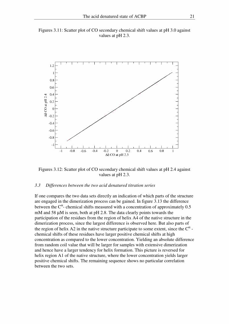
Figures 3.12: Scatter plot of CO secondary chemical shift values at pH 2.4 against
values at pH 2.3.
3.3 Differences between the two acid denatured titration series
If one compares the two data sets directly an indication of which parts of the structure
are engaged in the dimerization process can be gained. In figure 3.13 the difference
between the Cα- chemical shifts measured with a concentration of approximately 0.5
mM and 58 µM is seen, both at pH 2.8. The data clearly points towards the
participation of the residues from the region of helix A4 of the native structure in the
dimerization process, since the largest difference is observed here. But also parts of
the region of helix A2 in the native structure participate to some extent, since the Cα -
chemical shifts of these residues have larger positive chemical shifts at high
concentration as compared to the lower concentration. Yielding an absolute difference
from random coil value that will be larger for samples with extensive dimerization
and hence have a larger tendency for helix formation. This picture is reversed for
helix region A1 of the native structure, where the lower concentration yields larger
positive chemical shifts. The remaining sequence shows no particular correlation
between the two sets.

22 The acid denatured state of ACBP
Figure 3.13: Difference between C
α chemical shifts from the two data-series (0.5
mM data-set minus 58 µM data-set) at pH 2.8.
This difference between the two sets converges as the pH gets smaller, indicating that
the two sets move towards the same conformations, as the proteins get more unfolded,
see figure A.7 in Appendix A, showing the difference between the two sets at pH 2.3,
for both Cα and CO chemical shifts. The difference between the two titration series
suggest that the extent in helix formation in the region of A4 and A2 would be over-
estimated, while A1 would be underestimated in the high concentration pH titration
series, as compared to the actual extent present with no dimerization.
The influence the two different random-coil data have on the chemical shifts, both
values are obtained for small model peptides, but under different denaturant
conditions, is evaluated. As previously mentioned, the two random coil value datasets
were those from Wishart et al. [DWisha95] measured at pH = 5, in 1 M urea, and
Schwarzinger et al. [SSchwa01], where the model peptides were evaluated at pH = 2.3
in 8 M urea, both including nearest neighbour effects. Figures 3.14 and 3.15 show the
same data-set measured at low ACBP concentration obtained at pH 2.7 evaluated with
random coil values from Wishart et al. and Schwarzinger et al., respectively.
Differences are observed for the helix A1 region and the region from the middle of
A2 to the centre of A3, differences which most probably can be attributed to pH
effects on specific residues.
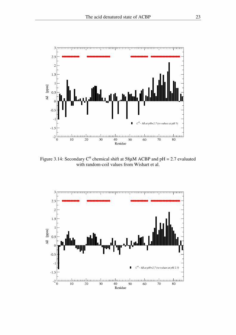
The acid denatured state of ACBP 23
Figure 3.14: Secondary C
α chemical shift at 58µM ACBP and pH = 2.7 evaluated
with random-coil values from Wishart et al.

24 The acid denatured state of ACBP
Figure 3.15: Secondary Cα chemical shift at 58µM ACBP and pH = 2.7 evaluated
with random-coil values from Schwarzinger et al.
In order to evaluate the influence of the two different random coil values on ACBP it
is possible to look at the difference the two datasets of random coil chemical shift
values have on the sequence of ACBP. This gives rise to, what one could call an
intrinsic pH dependency for ACBP, i.e. a sequence specific chemical shift
dependency on nearest neighbours and the pH-values. There is of course also a
difference in denaturant concentration. If one subtracts the random-coil values derived
from Wishart et al. for each residue of ACBP, from those assigned by Schwarzinger a
picture of the intrinsic pH dependency for ACBP emerges, see figures 3.16 and 3.17,
for Cα and CO respectively.
Figure 3.16: ACBP sequence specific random coil values for C
α, representing the
intrinsic pH dependency of ACBP (Wishart et al. minus Schwarzinger et al.
random-coil values). All large negative values are Asp residues.

The acid denatured state of ACBP 25
Figure 3:17: ACBP sequence specific random coil values for CO, representing the
intrinsic pH dependency of ACBP (Wishart et al. minus Schwarzinger et al.
random-coil values).
As is seen from figure 3.16, the dependency for Cα chemical shifts are evenly
distributed throughout the sequence, but might display a small correlation for the
second half of the A1, A2 regions and the loop in between, while CO exhibit a
clustering around A1 and the beginning of A2, figure 3.17. The positive difference for
residues, especially for the region from the middle of A2 to the centre of A3 for Cα
chemical shifts, figure 3.16, can for instance explain the distinction in appearance
observed in this region seen in figures 3.14 and 3.15. But also leads to a significant
absolute difference in chemical shifts for the regions comprising the helices in the
native structure. It is hence highly relevant which random coil values are used to
estimate the secondary chemical shifts in order to avoid an over- or under-estimation
of the extent of helix formation in the mentioned regions. For the data obtained here,
under denaturing conditions at low pH the random coil values obtained by
Schwarzinger et al. should be used, whereas data obtained around pH 5 should be
evaluated against the random coil values of Wishart et al.
3.4 Discussion/Conclusion
In summary ACBP forms more residual structure over the course of the pH-interval in
all four helix regions, with A4 being the region with the largest tendency for helix
formation in the acid unfolded state. To a lesser extent than helix A4, helix A2 is
formed, and even less A1 and A3. Which of the two last helices has the larger
tendency for helix is hard to determine, a feature that repeats itself for the CO
chemical shifts. The HN chemical shifts show the highest tendency of occurring in the

26 The acid denatured state of ACBP
region of helix A3, while A1 seems to be much less ordered for chemical shifts of this
nuclei-species, but amide hydrogen chemical shifts experience almost no change over
the course of the pH interval.
The NH
secondary chemical shifts demonstrated negative correlations away from
random-coil in all regions except the loops at low ACBP concentrations, which stood
in contrast to the unstructured pattern for the values obtained at high concentration of
ACBP. The linear regression data supported a change towards α-helix formation from
low to high pH in α-helix region A4.
These data confirm the previously obtained information about the folding of ACBP
(see chapter 2), which propose that folding of ACBP proceeds through the formation
of a rate-limiting transition state [KTeilu05]. Calculation of secondary structure
formation showed the highest propensity for α-helix to be in the peptide segment of
α-helix A4 of the native structure [KTeilu02], which is clearly corroborated by the
present chemical shift analysis, which even suggests residual secondary structure at
pH 2.3. Also hydrogen protection in the early stages of folding supported the
assumption of high α-helix propensity in A4 [KTeilu00] and further the view that
bovine ACBP undergoes transient helix formation in the region comprising helix A4
and that hydrophobic interactions between residues in A1, A2 and A4 form a
transition state.
Interestingly, the evaluation of the acid denaturing at two concentrations gave an
indication of the participation of residues of helix A4 in the native structure and to a
lesser extent A2, in the dimerization process. The increase in helical contents in A2
might be a passive effect due to presence of a more stable A4-region and not actually
infer the participation of residues of A2 in the dimerization process. Samples with
extensive dimerization will have a larger tendency for helix formation in those two
regions of the peptide sequence. This picture is reversed for helix region A1 of the
native structure, where there exists a bigger tendency for helix formation in samples
with no significant dimerization. Previous investigation of the dimerization of ACBP
and the peptide segment comprising helix A4, proved the cooperative association of
two denatured ACBP molecules to a homodimer mediated by the peptide segment
comprising helix A4 [WFiebe05]. Emphasising the role of A4 as a prime structural
element, which operates to stabilize the denatured state of ACBP. For one, by native-
like interactions with the region A2 and by non-native interactions like the formation
of the homodimer at higher protein concentrations. The role of helix A4 is similar to
that seen for helix H of apomyoglobin (see chapter 2, P. E. Wright and R. L. Baldwin
in [RPain00]), which also participates in the structure of the denatured state, as well as
in an intermediate state of the folding process and in the native state. But ACBP
exhibits much more residual structure in A4 in the denatured state [JThoms02] than
helix H.
In order to get a more quantitative measure of helix formation during the course of
acid denaturing, the data was studied by theoretical means, in the form of Molecular
Dynamic and Monte Carlo Simulations. For the evaluation of which helix has the
largest propensity, more importance is placed in the Cα-chemical shifts, since they
mostly depend on the sidechain, while NH, CO a very sequence depended (engage in
bond formation). But since carbonyl carbon chemical shifts exhibit a similar picture to
that obtained for Cα chemical shifts, emphasis in the Monte Carlo simulation is also
put on this nucleus.

Urea and Guanidine hydrochloride denaturation 27
4 Urea and Guanidine hydrochloride denaturation
Two other major denaturants used in the study of protein folding are urea and
guanidine hydrochloride (GuHCl). Both are considered less attractive than acid
denaturing due to their ability to bind to proteins [ELiepi94], [DShort01].
The exact molecular mechanism by which urea unfolds is unknown, other than an
altered protein-solvent interaction. It has, though, long been known that both
denaturants act by favouring the stabilization of the unfolded state in preference to the
native state [CTanfo68], [CNPace86]. I.e., raising the solubility of most parts of the
protein compared to water and hereby stabilizing the denatured state compared to the
native.
Denaturants like urea might bind directly to the protein surface or interrupt the
hydrophobic interaction due to altered solvent properties or a combination of both.
Both mechanisms are likely. The first requires the exposure of more binding sites in
the denaturing protein, while the other should destabilize the hydrophobic interactions
of the folded protein. Several studies have indicated the presents of short-lived
binding of urea to proteins and the relatively high concentration of denaturant indicate
the necessity of many binding sites [JSchel02], [ELiepi94]. Recently evidence for
weak binding of urea and GuHCl as being directed towards the backbone has been
seen for poly-glycine-serine chains [AMögli05]. The data indicated that both
denaturants act by increasing solvent viscosity by indirectly slowing chain dynamics,
as well as direct interaction with the polypeptide chain. The article additionally
attributed the dissimilarity in their ability to denature to the difference in binding
affinities, since they both exhibit the same number of denaturant binding sites along
the polypeptide backbone.
Furthermore, experimental evidence has also been seen [KModig03] for long-lived
(strong) binding of urea to intestinal fatty acid-binding protein, indicating site-specific
binding of urea to both the native, as well as to the denatured protein. Thus,
illustrating that strong binding adds to the unfolding. This in turn also gives that a
simple extrapolation from a urea concentration, were residual structure still is present,
to a higher concentration where the protein would be totally random coil, is not
possible.
Also MD simulations on peptides in urea suggest the participation of both the direct
and indirect mechanisms in the chemical denaturation process [ACabal05].
The interpretation of unfolded proteins is obscured by the use of chemical
denaturants, since the denaturants may have an effect on the spectral characteristics of
the unfolded protein, as well as on its conformational preference [CPace86]. This
makes it difficult to separate effects on for instants chemical shifts arising due to
residual structure from effects of the denaturant. Guanidine Hydrochlorides effect on
random coil chemical shifts has previously been studied by investigating the peptide
sequence GGXGG for all 20 amino acids in the case of proton chemical shifts
[KPlaxc97]. While the effect on 13
C and 15
N chemical shifts was investigated on
seven representative peptides, all at 20 degree, at pH 5 and referenced to internal
DSS. This study provided correction factors, enabling to subtract the effect of GuHCl
on the random coil chemical shifts.
They also showed that the intrinsic backbone conformational preferences of ϕ, ψ, and
ω were not affected by GuHCl, but showed that GuHCl had an effect on the chemical
shifts of referencing compounds, for instants that its effect on water was ∆δ = -0.044

28 Urea and Guanidine hydrochloride denaturation
ppm M-1
. The induced chemical shift changes were shown to be linearly dependent on
the GuHCl concentration. The largest effect of the denaturant was shown to arise in 15
N chemical shifts, but exhibited relatively small residue specific dispersion. Of the
carbon resonance, carbonyl carbons showed the largest sensitivity towards GuHCl,
but also showed a small residue specific dispersion, ∆δ = -0.086 ± 0.016 ppm M-1
,
while the effect on aliphatic carbons was relatively small but revealed a large
dependency on residue type. E.g. for Cα ∆δ equalled –0.038 ± 0.044 ppm M
-1. For this
reason the Cα chemical shifts investigated in this study were just corrected for the
seven investigated peptides, while carbonyl shifts were corrected for the seven known
as well as with the mean value for the unknown amino acids. However, those seven
peptides still comprised roughly 2⁄3 of ACBP’s amino acid sequence (Ala, Arg, Glu,
Iso, Leu, Lys, Thr, Tyr and Val). Plaxco et al. also found that hydrogen’s adjacent to
carbonyl carbons, as well as Hα resonance’s experienced relatively large changes,
which, together with the lack of disturbance on the peptide conformation, they
interpreted as evidence of GuHCl denaturant action as an effect on the hydrogen-
bonding interactions between the carbonyl oxygen’s, the amide protons and the
surrounding water. That is, supporting the hypothesis of changes to solvation
properties of water for GuHCl denaturing mechanism as opposed to specific binding.
The perception that denatured proteins are fully solvated random coils, is slowly been
revised due to extensive experimental evidence. Spectroscopic evidence mounts up
that native-like topologies persist under strong denaturants conditions, e.g. for urea
concentrations of at least 8 M [YLiFPi05], where residual structure also is observed
for low pH. Also small angle X-ray scattering show that some proteins exhibit
residual secondary structure even under strong denaturing conditions [JKohn04].

Urea and Guanidine hydrochloride denaturation 29
4.1 The urea denatured state
In order to get and truly random coil data set for the interpretation of the acid
denatured state, that is where ACBP has no residual secondary structure, a titration by
urea was made at concentrations of 1.1, 2.1, 3.1, 4.1 and 5.1 M. The samples were
adjusted to pH 2.3, in 10 mM Glycine buffer, 10% D2O and a concentration of ACBP
of 60 µM. The urea concentration interval was decided on after a urea denaturation
with CD-spectroscopy in the far UV-region from 195 to 230 nm, where ACBP was
denatured in the interval from 0.86 M to 4.04 M urea at pH 2.3 and a concentration of
ACBP of roughly 20 µM. Over this interval the characteristic minima of a α-helix
secondary structure was reduced in magnitude by a factor of approximately four, and
its features almost totally extinguished.
At the investigated field strengths in NMR spectroscopy, the water and urea peaks
exchange, making a direct classification of the direct and indirect reference value
impossible, since the proton transmitter offset frequency (tof) was shifted but
appeared to be unchanged due to the exchange with urea. In order to subsequently
calculate the correct reference values for the three nuclei, DSS (3-(Trimethylsilyl)-1-
propanesulfonic acid Sodium salt) was used as an internal standard. See Appendix C
for a table of measured and revised proton transmitter offsets (tof’s), table C.1.
It was not possible to follow all residues from previously assigned peaks at pH 2.3
and 0 M to 1 M urea, therefore spectra of HNCOCA and HNCACB also were
recorded.
Unfortunately the chemical shifts of Cα and CO did not completely go towards
random coil values in the chosen urea concentration interval. Figure 4.1 shows a
segment of CO chemical shifts of all 5 concentrations projected into one 15
N plane.
As can be seen for the residues Glu-60 and Ala-57, they are located far from their
respective random coil values, although they converge slightly towards them during
the course from 1 to 5 M urea. Lys-66 and Ile-39 are just slightly off set from there
random-coil value, and could therefore be regarded as moving closer to their random
coil value, whereas Val-36 does not change much over the concentration range and
hence does not converge towards its random-coil value. Val-36 could be considered
totally unstructured and suggest an inherent random coil value for ACBP. It is,
however, also just slightly offset from its random coil value, which could be due to
binding of urea. Lys-52 is also offset from its random coil value, and does due to the
offset not seem to move closer to it. This represents it self in figure 4.3 by a change in
sign of the CO secondary chemical shift. A feature that is also observed for other
residues, both carbonyl and Cα chemical shift, see figures 4.2 and 4.3, e.g. residues
10, 27, 47, 53 and 79. All in all it can be seen, that all values exhibit an offset from
the standard random coil values, which can be both in the 13
C and/or 1H chemical shift
dimension. It is also noticed that this offset factor is not the same for each residue.

30 Urea and Guanidine hydrochloride denaturation
Figure 4.1: CO chemical shifts projected into one
15N plane. The following peak
colours correspond to these different urea concentrations; black: 5 M, red: 4 M, green:
3M, blue: 2M and magenta: 1M. The different residues are denoted by there three-
letter code and number in ACBP’s sequence, with larger font compared to an “x” and
Res-#, which denotes the location of that amino acids random coil value. Arrows
indicate the movement of a particular amino acid during the urea titration; the two red
arrows indicate Lys-52 movement passed its random-coil value.
Figure 4.2 and 4.3 show the secondary chemical shifts for Cα and CO, where again
the random coil chemical shift values from Schwarzinger et al. were used. Figure 4.2
shows that there still exist offsets from random coil values at 5 M urea in the areas of
helix A4, A1 and A2 in the native structure. The region of A4 is, as was also the case
for the acid denaturation, the segment of the peptide sequence that exhibits the largest
divergence from random-coil, followed by A1 and A2. As can be seen for several
residues, the chemical shifts go pass the random coil value, shifting from positive to
negative chemical shift differences, see for example residues 10, 11, 22, 45 and 78 to
82. Some segments of the peptide chain seem, however, not to change and might be
considered to represent the unstructured chain, e.g. residues 13-20 and 38-44, but
again the systematic offset should give rise to concerns.

Urea and Guanidine hydrochloride denaturation 31
Figure 4.2: C
α secondary chemical shifts for urea concentrations from 1.1 to 5.1.
black: 1 M, red: 2 M, green: 3 M, blue: 4 M and magenta: 5 M
A similar picture is seen for the carbonyl secondary chemical shifts, figure 4.3, where
the peptide segment of helix A4 in native structure also has the largest offset from
random coil and the largest change over the titration range, followed by A1.
Interestingly, A2 and A3 move further away from random coil over the concentration
range, whereas the loop region, especially around the start and end almost do not
change at all. Again this can be due to the offset, as well as areas that might be
regarded as unstructured.

32 Urea and Guanidine hydrochloride denaturation
Figure 4.3: CO secondary chemical shifts for urea concentrations from 1.1 to 5.1.
black: 1 M, red: 2 M, green: 3 M, blue: 4 M and yellow: 5 M
In Appendix C, figure C.1, a graph can be seen where the difference of Cα and CO
chemical shifts between 1M and 5M urea as a function of residue is depicted.
Indicating, that the largest changes over the titration range are seen in the region of
A4, followed by A2 and A1. Note, there might exist a factor like binding, which could
influence distinct areas of the peptide sequence differently, and hence make a
straightforward interpretation impossible. Changes over the titration range seem to
correlate relatively well between the two 13
C chemical shifts for the different
segments of the polypeptide chain. It is such that the difference of CO chemical shifts
from 1M to 5M urea depicted against those for Cα chemical shifts exhibit a
correlation coefficient of 0.87, see figure 4.4.

Urea and Guanidine hydrochloride denaturation 33
Figure 4.4: CO chemical shift differences (1M minus 5M urea) depicted against C
α
chemical shift differences for the same interval. The correlation coefficient equals
0.87.
Several studies, as discussed in chapter 4, have indicated the presence of residual
secondary structure in the presence of strong denaturant conditions of urea. But due to
the apparent offset it cannot be clearly said, that there exist residual secondary
structure at 5 M urea in the case of ACBP. It can, however, be concluded that the
peptide segment corresponding to helix A4 in the native structure still changes over
the titration range.
This offset can be interpreted as a binding effect of urea to the protein, as discussed in
chapter 4. This behaviour, regrettably, makes it impossible to extrapolate the slope
towards a 100 % denatured chemical shift distribution for ACBP.
If one measured the binding constant for urea to a random-coil model peptide, for
instance the helical regions of ACBP, it might be possible to take the binding of urea
to ACBP into account and extrapolate to random-coil values specific for ACBP.
Backbone chemical shift measurements on the peptide sequence comprising helix A3
in the native structure revealed that the chemical shifts in this peptide are very similar
over the range of urea concentrations to the one of the full length protein measured
here - except for some minor deviations in the N- and C- terminal residues
(measurements made by BBK). So it seems that the intrinsic behaviour of the
chemical shifts away from random coil values like Schwarzinger et al. are inherent
even to smaller peptides comprising the helices. Therefore smaller peptides from
ACBP’s sequence cannot as such be used as “random coil” values.
In Appendix C figures of the behaviour of the amide proton and nitrogen chemical
shifts during the titration experiment can be seen, figures C.2, C.3. The amide

34 Urea and Guanidine hydrochloride denaturation
nitrogen chemical shifts do not change much over the range of urea concentrations,
but exhibit large off-sets up to ± 3 ppm from the random coil values of Schwarzinger
et al., where the loop residues seem to be responsible for the largest positive off-sets.
A feature that is not repeated for the amide proton secondary chemical shifts, figure
C.3. The amide proton secondary chemical shifts show the same pattern with largest
offsets from random coil in the regions of helices A4, part of A3, A2 and A1 in the
native structure. These changes, however, are not huge over the interval form 1 to 5 M
urea, but with the largest changes observed in the regions A4, A2 and A1.

Urea and Guanidine hydrochloride denaturation 35
4.2 The Guanidine hydrochloride denatured state
ACBP was also denatured by guanidine hydrochloride (GuHCl). It is believed that the
mechanism by which GuHCl disrupts the structure and unfolds a protein arises by
changing the solvation properties of water as mentioned in chapter 4 [KPlaxc97].
Urea denaturation, on the other hand, is thought to arise both due to direct binding as
well as a result of changed solvation properties. Here the unfolding of ACBP by
GuHCl was investigated in order to compare different chemical denaturations of
ACBP and reveal eventual differences in the unfolding of ACBP.
Again the backbone chemical shifts CO, HN, NH of 13
C, 15
N double-labelled bovine
ACBP in 10% D2O, were measured. ACBP’s concentration was approximately 0.5
mM, the same as the high concentration pH titration series. Investigations [WFiebe05]
didn’t reveal any dimerization effects of ACBP for denaturation in GuHCl, which
made it possible to use a high concentration of the protein. The following
concentrations were investigated: 2.5, 3.47, 4.06, 4.67, 5.15 and 5.51 M at a pH of 5.3
and every GuHCl concentration was verified by refractrometry [YNozak72].
As pointed out in chapter 4, GuHCl has a marked influence on random coil chemical
shift of model peptides, as well as an evident effect on reference compounds.
Therefore all chemical shifts were corrected for these effects. The chemical shift
change of DSS was measured externally at O M and at 5.05 M GuHCl, under the
same experimental conditions as the data collection, with a 13
C-HSQC-spectrum. Due
to the linear dependence of GuHCl on water and DSS, this gave rise to a correction
factor for 1H of 0.051 ppm M
-1 and by indirect referencing, 0.05 ppm M
-1 for C
α and
0.04 ppm M-1
for CO. Interestingly, this is an effect of GuHCl on DSS and water and
not an indirect effect of GuHCl due to instrumental/experimental set-up, as was the
case for urea, were urea and water were in fast exchange hiding a change in the
resonance frequency of water. GuHCl and water are under the investigated
experimental conditions in slow exchange and the 5 labile protons exhibit one single
peak at a frequency of 6.76 ppm in 5.05 M GuHCl.
Furthermore the secondary chemical shifts were corrected for the effect of GuHCl on
the random coil chemical shifts, see chapter 4. As mentioned in the same chapter,
carbonyl shifts were corrected for all amino acids in the peptide sequence of ACBP,
where amino acids not investigated by Plaxco et al. [KPlaxc97] were approximated by
the mean value of ∆δ = -0.086 ± 0.016 ppm M-1
. Whereas, Cα secondary chemical
shifts just were corrected for the known amino acids, due to their large residue
specific dependence on GuHCl, ∆δ = –0.038 ± 0.044 ppm M-1
. But these seven
investigated residues still made up for roughly 2⁄3 of the amino acids of ACBP.
Figures 4.5 and 4.6 show the secondary chemical shifts of Cα and CO at 3.47 and 5.5
M GuHCl. Both are corrected for the action of GuHCl on the random coil shifts, as
well as on the referencing compound as described above. The secondary Cα chemical
shift are almost all positive at 3.47 M and get smaller and some negative as the
concentration rises to 5.51 M GuHCl, some thereby “surpassing” the random coil
chemical shift, which in the case for the GuHCl titration series was based on Wishart
et al. [DWisha95]. No apparent pattern, similar to the one found in acid denaturing
series, is seen, see figure 4.5. The carbonyl shifts are almost exclusively negative at
both concentrations and get more negative as the concentrations is raised, see figure
4.6. Again, no pattern is immediately evident, suggesting the same unstructured
polypeptide chain.

36 Urea and Guanidine hydrochloride denaturation
Figure 4.5: C
α secondary chemical shifts at 3.47 and 5.51 M GuHCl, red solid bars
and open blue bars, respectively, as function of residue number. Corrected for the
action of GuHCl on the random coil shifts, as well as on the referencing compound.

Urea and Guanidine hydrochloride denaturation 37
Figure 4.6: CO secondary chemical shifts at 3.47 and 5.51 M GuHCl, red solid bars
and open blue bars, respectively, as function of residue number. Corrected for the
action of GuHCl on the random coil shifts, as well as on the referencing compound.
Figures 4.7 and 4.8 show the chemical shift difference per molar GuHCl as found by
linear regression for the aliphatic Cα carbon. In these calculations the x-axis had the
same direction as was used for the pH-titration series, that is from most unfolded to
less unfolded (5.5 M → 2.5 M). The error bars in figure 4.7 indicate the standard
deviation from this slope for each residue and represent the raw data not corrected for
the effect of GuHCl on the random coil values and its effect on DSS. Figure 4.8
shows the same data corrected for the effect of GuHCl. As is clearly seen, the
chemical shift pattern between the two figures is quite dissimilar. The data in figure
4.7 encourages the perception of structural loss in the peptide segment of helix A4 in
the native structure and figure 4.8 supports and strengthens this view, but also shows a
reduction in the region A2. The data measured here supports the finding of residual
structure in A4 and A2, but to a much lesser extent and not as obviously as the
findings in the acid denatured state. For instance, the approximate change in Cα
secondary chemical shift pr mole GuHCl is just 0.05 ppm, whereas the same change
in the acid-unfolded state is roughly 0.4 ppm.
Figure 4.7: C
α chemical shift difference per molar GuHCl in the interval from 2.5
to 5.51 M with standard deviation, not corrected for the effects of GuHCl on the
random coil shifts and DSS.

38 Urea and Guanidine hydrochloride denaturation
Figure 4.8: C
α chemical shift difference per molar GuHCl in the interval from 2.5
to 5.51 M, corrected for the effects of GuHCl on the random coil shifts and DSS.
The behaviour of the carbonyl shifts are actually quite different from those observed
for the Cα chemical shifts. Figures 4.9 and 4.10 show the chemical shift difference per
molar GuHCl as found by linear regression for the carbonyl shifts. The error bars
indicate the standard deviation from this slope for each residue. Figure 4.9 shows the
raw data, while figure 4.10 is corrected for the effect GuHCl has on the random coil
values, as well as on DSS. The huge difference in appearance between the two figures
makes the necessity of correction for GuHCl intrinsic effects on the polypeptide chain
very clear. While the first figure may indicate apparent residual secondary structure
in A2 and A4, figure 4.10 may just very vaguely indicate differences between the
changes in chemical shifts over the investigated GuHCl concentrations. The changes
in chemical shifts are fractionally more pronounced in the first half of A2, compared
to the surrounding loops and helices. A very small difference compared to the
surrounding residues can also be observed for the last two-third of helix A4.

Urea and Guanidine hydrochloride denaturation 39
Figure 4.9: CO chemical shift difference per molar GuHCl in the interval from 3.47
to 5.51 M with standard deviation, not corrected for the effects of GuHCl on the
random coil shifts and DSS.

40 Urea and Guanidine hydrochloride denaturation
Figure 4.10: CO chemical shift difference per molar GuHCl in the interval from 2.5
to 5.51 M, corrected for the effects of GuHCl on the random coil shifts and DSS.
This striking difference between Cα and CO chemical shifts is not observed under the
other denaturing conditions investigated. This could be an indication of a difference in
denaturing mechanism and might even be attributed to a change in hydrogen-bonding
interactions between the carbonyl oxygen’s, the amide protons and the surrounding
water, since the effect of GuHCl was believed to be one of changed solvation
properties of the solvent [KPlaxc97]. Plaxco et al. also argues that the effect GuHCl
has on the chemical shifts is not simply an effect of increased ionic strength, since
sodium chloride at high concentration does not affect proton chemical shifts the way
GuHCl does.
As mentioned in chapter 2, the unfolding/folding pathway of CI2 exhibits a single
rate-determining transition state ensemble for folding and unfolding [VDagge03].
Chymotrypsin inhibitor 2 (CI2) unfolding by guanidinum chloride (6.4 M) showed
most of the nuclei having chemical shifts close to random coil values except for two
short peptides segments of a total of 10 residues, suggesting residual structure in a
otherwise highly unfolded protein [SKazmi01]. MD-simulations support the findings
of an expanded poorly structured denatured state with residual native helical structure
in the denatured state of CI2. But CI2 seems to have much less pronounces residual
structure in the GuHCl denatured state than the data for ACBP suggest (10 residues
compared to the two regions A4 and A2 in ACBP).
Previously the backbone 15
N and 1H
N chemical shifts of a mutant (I86C) of ACBP
were investigated in GuHCl from 1.9 M to 4 M, indicating no cooperative transitions.
However, these measurements were not corrected for the effects of GuHCl on the
random coil values [KTeilu02]. The carbon resonance Cα, C
β and CO were evaluated
at 1.9 M and revealed small deviation from random coil values, indicating small
amounts of residual structure, but were again not corrected for the effect of GuHCl.
The results here strengthen the view of residual structure in the peptide segments
comprising helix A4 and A2 of the native structure even under strong denaturant
conditions.

Assessing the ensemble of structures representing the denatured state 41
5 Assessing the ensemble of structures representing the denatured state
NMR-data obtained of the denatured states of macromolecules comprise of an
average over a broad range of structures and it is hence, not possible to deduce
something about the structures given rise to the experimental data without the use of
computational approaches. That is, standard structure determination procedures
cannot be applied to the denatured state.
Simple folding models, assuming that only interactions of the native state are
favourable and ignoring non-native interactions, can predict folding rates, distribution
of transition state ensembles and structures of the native state for small proteins
relatively well [DBaker00]. These models are based on the assumption that the
general path of the polypeptide chain during folding is determined by its topology
rather than inter-atomic interactions [EAlm99].
Computational approaches on unfolded states have previously been implemented,
where experimental data are compared to averages calculated over ensembles of
structures [WChoy01]. Experimental data like paramagnetic relaxation enhancement
have been use as distance restraints in computer simulation in order to determine the
conformational ensembles representing the denatured state of ACBP. These
simulations suggest the interaction of N and C-terminal parts of the protein sequence
in the denatured state [SKrist05]. Paramagnetic relaxation enhancement derived
distance restraints were also enforced on the average distance calculated across
simulated ensembles, indicating the presence of residual structure and long-range
interaction in the denatured state of ACBP [KLLars04].
The basic idea for the computational approach used here, is a two-stage approach
were the experimental data are compared to averages calculated over an ensemble of
structures. First an appropriate ensemble of initial structures is generated. This
ensemble is generated by molecular dynamics simulations, where the equivalence
between time and ensemble averages in sufficient long simulation is exploited.
Different dihedral (ϕ, ψ) restraints on different areas of the unfolded structure of
ACBP are applied, trying to encompass different aspects of the experimental data. For
those structures, 140.000 in total, chemical shift data are calculated by the semi-
empirical computer program SHIFTX [SNeal03], which again are used as restraints in
Monte Carlo simulations, where the final ensemble is found by an energy
minimization between the experimental and calculated chemical shift data. I.e. the
initial ensemble of 140.000 structures is sampled by Monte Carlo simulations, which
represent the second stage of the computational approach.
One problem of this approach is that the right ensemble comprising the experimental
data, and hence simulating reality, is only found if adequate structures are present in
the initial ensemble.
5.1 Molecular Dynamics Simulations
Molecular Dynamics Simulations, MD-simulations for short, can be used for
theoretical studies of biological systems. MD-simulations calculate time dependent
behaviour and can hence give detailed information on fluctuations and conformational
changes of for instance proteins. Molecular Dynamics Simulations produce
information such as the systems atomic positions and velocities, were a time series
yield an ensemble of structures, which exhibit the same thermodynamic state.

42 Assessing the ensemble of structures representing the denatured state
The theory behind Molecular dynamics simulations is based on Newton’s second law,
and yields position, velocities and acceleration of each particle. From an initial state
and with the potential energy function the trajectory for the system can be calculated.
The potential energy function is rather complex for large systems, and must therefore
be solved numerically. Several algorithms exist for the integration of the equations for
motion; here the Leap-frog algorithm (velocities and position are not calculated at the
same time) were used in the simulations.
5.1.1 CHARMM Force Field
The potential energy function, or force field, is a compromise between accuracy and
computational cost (with respect to ab initio methods), and is often calibrated against
experimental results and quantum mechanical calculations on small model
compounds. A force field does not allow for changes in electronic structure, as bond
making or breaking, as compared to quantum mechanical methods. For the
simulations of unfolded ACBP the CHARMM force field (Chemistry HARvard
Molecular Mechanics) was used. This potential energy function is calculated as a sum
of internal terms (Ebonded) and external terms (Enon-bonded), equation 5.1. The first
describes bonds, angles and bond rotations in the molecule, while the second
represents the non-bonded atoms and atoms separated by three or more covalent
bonds.
43421321Waalsdervanticelectrostarotationbondbendinganglestretchingbond EE
bondednon
EEE
bonded EERV
−−−−− +
−
++
+=)( ,
5.1
where R is the atom position.
( ) ( ) ( )[ ] ∑∑ ∑∑∑+==+==
−+
+−+−+−=
N
iji ij
ij
ij
ij
bonds
N
iji ij
ji
torsionsangles
br
C
r
A
Dr
qqnKKbbKRV
1,1612
1,1
2
0
2
0 cos1)( φθθ φθ
5.2
V(R) is a function of the position of N particles and the first term models the
interaction between pairs of bonded atoms via a harmonic potential, where the energy
increases as the bond length b deviates from a reference bond length b0 and where Kb
is a force constant, which depends on the type of atoms involved. The second term
describes in the same way by a harmonic potential the alteration of the bond angles
from an ideal value θ0, while the last of the bonded terms is modelled by a periodic
function describing how the energy changes as a bond rotates (torsions), see equation
5.2.
In addition the CHARMM force field contains two terms representing an interaction
based on the distance between atoms separated by two bonds (the Urey-Bradley term)
and a term used to preserve planarity and chirality (the improper dihedral term).
The two non-bonded terms represent the electrostatic and van der Walls interactions
of the atoms. The electrostatic interaction is given by the Coulomb potential, where D
is the effective dielectric function and r is the distance between the two charges. The
Van der Waals interactions are generally described by the Lennard-Jones 12-6
potential. In order to simplify calculations a fixed set of atoms types is used, e.g. an
aliphatic carbon atom in sp3 bonding situation differs from a carbon in a ring,
minimizing the number of possibilities. To facilitate faster computations a pair-wise
additive approach is used as well, meaning a pair of atoms do not feel the interaction
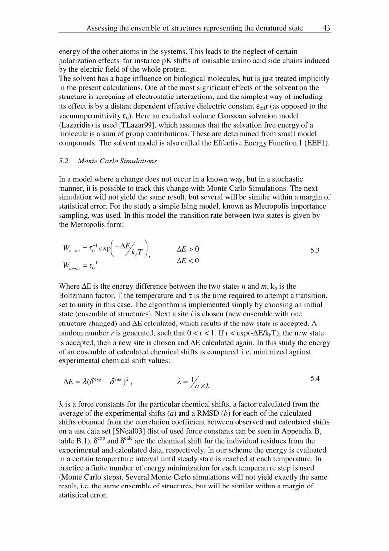
Assessing the ensemble of structures representing the denatured state 43
energy of the other atoms in the systems. This leads to the neglect of certain
polarization effects, for instance pK shifts of ionisable amino acid side chains induced
by the electric field of the whole protein.
The solvent has a huge influence on biological molecules, but is just treated implicitly
in the present calculations. One of the most significant effects of the solvent on the
structure is screening of electrostatic interactions, and the simplest way of including
its effect is by a distant dependent effective dielectric constant εeffr (as opposed to the
vacuumpermittivity εo). Here an excluded volume Gaussian solvation model
(Lazaridis) is used [TLazar99], which assumes that the solvation free energy of a
molecule is a sum of group contributions. These are determined from small model
compounds. The solvent model is also called the Effective Energy Function 1 (EEF1).
5.2 Monte Carlo Simulations
In a model where a change does not occur in a known way, but in a stochastic
manner, it is possible to track this change with Monte Carlo Simulations. The next
simulation will not yield the same result, but several will be similar within a margin of
statistical error. For the study a simple Ising model, known as Metropolis importance
sampling, was used. In this model the transition rate between two states is given by
the Metropolis form:
1
0
1
0 exp
−→
−→
=
∆−=
τ
τ
mn
bmn
W
TkEW
, 0
0
<∆
>∆
E
E
5.3
Where ∆E is the energy difference between the two states n and m, kb is the
Boltzmann factor, T the temperature and τ is the time required to attempt a transition,
set to unity in this case. The algorithm is implemented simply by choosing an initial
state (ensemble of structures). Next a site i is chosen (new ensemble with one
structure changed) and ∆E calculated, which results if the new state is accepted. A
random number r is generated, such that 0 < r < 1. If r < exp(-∆E/kbT), the new state
is accepted, then a new site is chosen and ∆E calculated again. In this study the energy
of an ensemble of calculated chemical shifts is compared, i.e. minimized against
experimental chemical shift values:
2exp )( calcE δδλ −=∆ ,
ba ×= 1λ 5.4
λ is a force constants for the particular chemical shifts, a factor calculated from the
average of the experimental shifts (a) and a RMSD (b) for each of the calculated
shifts obtained from the correlation coefficient between observed and calculated shifts
on a test data set [SNeal03] (list of used force constants can be seen in Appendix B,
table B.1). δexp and δcalc
are the chemical shift for the individual residues from the
experimental and calculated data, respectively. In our scheme the energy is evaluated
in a certain temperature interval until steady state is reached at each temperature. In
practice a finite number of energy minimization for each temperature step is used
(Monte Carlo steps). Several Monte Carlo simulations will not yield exactly the same
result, i.e. the same ensemble of structures, but will be similar within a margin of
statistical error.

44 Assessing the ensemble of structures representing the denatured state
5.3 SHIFTX
The calculated chemical shift data was created on the basis of the program SHIFTX
[SNeal03]. The program calculates the diamagnetic 1H,
13C and
15N chemical shifts
for both backbone and sidechain atoms of proteins. Here the simulated structures
derived from the MD simulations were used as input structures. The program predicts
the chemical shifts from atomic coordinates by using classical and semi-classical
equations for ring-currents, electric field, hydrogen bond and solvent effects as well as
pre-determined empirically derived chemical shift hypersurfaces. The chemical shift
hypersurfaces were created via a database of protein chemical shifts and high-
resolution X-ray structures and describe effects such as nearest neighbour effects,
secondary structure, sidechain orientations and dihedral angles, which are difficult to
express analytically or predict classically. For folded proteins the program achieves
very good correlations between calculated and observed shifts, making the program
applicable for structure refinement in NMR (Correlation coefficients and RMSD for
each atom type can be found in Appendix B, table B.1).
5.4 PALES
The program PALES [MZweck00] can be used for the analysis of residual dipolar
couplings, and mainly simulates the magnitude and orientation of a sterically induced
alignment tensor from a solutes three-dimensional structure. PALES makes a
systematic search of the solutes orientations that get obstructed by the alignment
media and calculates the averages of all individual alignment tensors for the
remaining non-obstructed molecules. In the PALES program it is assumed that
alignment occurs in a liquid crystaline phase where no major attractive or long range
repulsive interactions take place between the solute and the obstructing particles, i.e.
only steric alignment. PALES calculates/predicts residual dipolar couplings (RDC)
from pdb-files, and uses experimentally derived dipolar couplings as start values.

Molecular Dynamics and Monte Carlo Simulations results 45
6 Molecular Dynamics and Monte Carlo Simulations results
In order to evaluate the chemical shift data obtained in the acid denaturing titration
series Molecular Dynamic and Monte Carlo simulations where performed. The
experimental data indicated the formation of secondary helical structure, see chapter
3. It is not believed that this residual secondary structure would appear in ordinary
Molecular Dynamic simulations. It is therefore necessary to introduce secondary
structure by means of restraining ϕ, ψ angles to appropriate values for helix. With
Molecular Dynamics simulations (MD) a set of 140.000 structures were constructed
with different extent of restrictions in different parts of the peptide sequence,
including 10.000 structures with no restriction at all, an ensemble that as well served
as random-coil values for the calculated data. This large ensemble thereby also
contains structures that represent unfolded ACBP. For all of these structures the
theoretical chemical shift (δ) were calculated by the program SHIFTX [SNeal03]. The
approach used here is a two-stage approach, where the first part consists of the
production of a large ensemble of 140.000 structures. In the second stage of the
approach the large ensemble is sampled with simulated annealing (SA), a Monte
Carlo method that enables “uphill” jumps out of local minima, see chapter 5 and
equation 5.3. This Metropolis procedure generates an ensemble at some specific
temperature; the SA approach “melts” the system at this temperature until no further
changes occur, then proceeding to a lower temperature [SKirkp83]. At each
temperature the simulation must continue long enough for the system to reach steady
state, i.e. no changes in the energy happen, see chapter 5, MC-simulation. This
energy is governed by the difference between experimental chemical shifts and
calculated chemical shifts. The MC-simulations therefore produce a sub-ensemble
that describes the experimental data. The found sub-ensemble is subsequently
analysed, among other properties, for secondary structure contents.
6.1 Molecular Dynamic Simulation: Construction, energy minimization
The initial unfolded structure of ACBP consisted of an all-atom ACBP peptide
sequence, i.e. which contains all heavy atoms as well as hydrogen atoms bound to
polar (O, S, N) heavy atoms. In order to construct the start ensemble of the 140.000
structures, 14 different MD-simulations were made, each sub-run comprising the
restraining of different areas of the four α-helical regions of the native structure of
ACBP. The different segments of the peptide sequence were restrained by forcing ϕ -
and ψ - angles of specific residues to uphold values close to those observed for
helices. The energy of each initial structure was minimized by methods of Steepest
Descend and Adopted Basis Newton-Raphson. The MD simulations with the
CHARMM19/EEF1 model were run for 40 ns and made at 573 K. The protein was
previously heated from 0 to 573 K in steps of 10 K. During the simulation 10.000
structures were saved (every 2000 steps). For these pdb-files were calculated and used
as input for SHIFTX.
For each MD-run both ϕ and ψ dihedral angles were constrained to values in the
vicinity of helix as given by the Ramachandran plot (an example of a restraint input
can be seen in Appendix B, table B.2). In order not to constrain the different parts too
tightly, thereby forcing the peptide segment into a α-helix with something resembling

46 Molecular Dynamics and Monte Carlo Simulations results
stable tertiary connections, the width of the angles, which the structures were allowed
to adopt and the penalty for violation (Force), were optimized so that the resulting
structures yielded an approximate α-helical content of 30%. The secondary structure
contents were calculated with the program DSSPcont [WKabsc83], [CAnder02] over
an average of 1000 structures. Figure 6.1 shows α-helical content, as calculated by
DSSPcont, as a function of the force, for several restraint residues over an ensemble
of structures from MD simulation where the dihedral angles ϕ,ψ were –62 ± 10 and –
41 ± 7.5. Figure 6.2 shows the α-helical contents as a function of the width for the
same residues at a force of 2.0 kcal/mol. In these simulations the four mid-residues in
each helix were constrained.
Figure 6.1: α-helical contents versus force for certain residues as found by
DSSPcont. The four mid-residues in each helix of the native structure were
constrained with dihedral angles ϕ,ψ [–62 ± 10] and [–41 ± 7.5]. The standard
deviation for residue 9 is shown.

Molecular Dynamics and Monte Carlo Simulations results 47
Figure 6.2 α-helical contents as a function of the width for ϕa
for certain residues as
found by DSSPcont. The four mid-residues in each helix were constrained, and the
force in each simulation was 2.0 kcal/mol. a: the widths of ϕ,ψ were simultaneously increased proportionally ([0,0], [1,0.5], [3,2], [9,6], [18,12],
[24,16], [36,24], [72,48])
All restraints were due to the above optimization consequently set to –62 ± 45 and –
41 ± 30 for ϕ and ψ respectively, while the force was held at 2.0 kcal/mol, in order to
obtain an approximate α-helical content of 30%. A picture of the secondary structure
contents at ϕ,ψ [–62 ± 10] and [–41 ± 7.5] and a force of 2.0 kcal/mol can be found in
Appendix B, figure B.1. The different areas that were constrained, in order to
construct the start ensemble of 140.000 structures for a suitable representation of
unfolded ACBP, can be seen in table 6.1.
The residues chosen to be restrained were selected on the bases of the chemical shift
pattern obtained in the experimental data for Cα and CO chemical shifts. For instance,
the first and last residues in each helix of the native structure were not in all cases
restrained, since they did not seem to change over the course of the pH-interval and
did not deviate much from random coil values. That is, the experimental results from
the NMR experiments were used as a guide to decide which dihedral angles should be
restraint in the MD-simulations, see for instance figures 3.5 and 3.6.
The resulting pdb-files were used as input for SHIFTX to calculated theoretical
chemical shifts. Examples of the average chemical shift as calculated by SHIFTX for
1000 structures where 4 residues in each helix were constrained can be seen for Cα
and carbonyl chemical shifts in Appendix B, figures B.2 and B.3.

48 Molecular Dynamics and Monte Carlo Simulations results
Table 6.1.
Restraint-bin Helix Residues
1 A4 aa66 - aa83
2 A2 aa22 - aa35
3 A4 & A2 aa22 - aa35 & aa66 – aa83
4 A3 aa52 - aa61
5 A1 aa4 - aa14
6 A4, A2 & A3 aa22 - aa35, aa52 - aa61 & aa66 - aa83
7 ½ A2 aa29 – aa35
8 3⁄4 A4 aa66 – aa79
9 ½ A2 & 3⁄4 A4 aa29 – aa35 & aa66 – aa79
10 A4 aa65 – aa84
11 A2 aa21 –aa36
12 A4 & A2 aa21 –aa36 & aa65 – aa84
13 no restraints -
14 ½ A2 aa22 – aa26
The ensembles of the 140.000 structures hence include structures with helix in
different parts of the peptide sequence. Each Restraint-bin of table 6.1 represents
structures where a particular area of the peptide sequence 30 % of the time exhibits α-
helical structure. I.e. 70 % of the time or rather 70 % of the structures, due to the
equivalence between time and ensemble averages, exhibit other conformations. For a
particular Restraint-bin the rest of the peptide sequence, apart from the residues
restraint, do not represent specific structures as well. The start ensemble also includes
at least 10.000 structures, which represent the unfolded peptide chain of ACBP.
In summary, the first stage comprised the construction of 140.000 structures of ACBP
by 14 Molecular Dynamic simulations. In 13 MD-runs out of the 14, each generating
10.000 structures, specific regions of ACBP’s sequence where constrained in order to
yield an overall α-helical content of 30 %. For all 140.000 structures pdb-files where
calculated and used as input for SHIFTX, thereby generating calculated chemical shift
data for 140.000 structures.
6.2 Monte Carlo simulations
The second stage of the computational approach comprised the sampling of the
140.000 structures by simulated annealing. The simulated annealing algorithm is
implemented by choosing an ensemble; in this study the simulated ensemble
comprised 10.000 structures. The energy for this state is calculated, where the energy
is the difference between the experimental and calculated chemical shift for each
residue, see equation 5.4. The next step is the replacement of one structure of this
ensemble with another from the ensemble of 140.000 structures produced by the MD
simulations and the calculation of the energy for this new state. If the energy
difference between these two states fulfils the scheme describe in chapter 5 the new
state is accepted. This sampling is repeated until the system reaches steady state at
each temperature and the energy is converged.
For Cα, CO, H
N and N
H chemical shifts the Monte Carlo simulations were optimized
varying the temperature interval in which the energy was minimized and number of
Monte Carlo steps at each temperature. I.e. the energy at each Monte Carlo step was
calculated as the difference between experimental chemical shifts and those calculated

Molecular Dynamics and Monte Carlo Simulations results 49
for 10.000 structures picked out of the 140.000 structure large start ensemble. This
resulted in the energy stabilizing and minimization of the difference between the
experimental and theoretical chemical shifts. In Appendix B examples of a trajectory
of the energy and the difference between experimental and calculated shifts for CO
and Cα are shown, figures B.4, B.5 and B.6. The optimal temperature interval for both
Cα and CO was found to be from 0.1 to 0.00001 in steps of 40, with 60 million Monte
Carlo steps at each temperature.
The simulated ensemble size was set to contain 10.000 structures, in order to sample a
sufficient ensemble size, but at the same time contain the amount of CPU time used
and make calculations feasible.
The experimental chemical shifts were those obtained during the pH-titration
experiments at low ACBP concentration from chapter 3. Due to the slow exchange
between peaks from the unfolded and folded populations, all simulations are hence
performed against the unfolded population.
The chemical shifts used in the energy minimization where secondary chemical shifts,
since the absolute chemical shifts yielded a bias producing much more helix all over
the amino acid sequence in order to minimize the energy. Since, the difference
between the experimental and calculated data were shifted toward positive values all
over the amino acid sequence, it seemed to be a general problem for the simulation. It
was believed that this arose due to an offset between the experimental chemical shifts
and the random-coil values for the calculated ensemble, i.e. Restraint-bin 13. In the
Monte Carlo simulations this would lead to more helical structures and no structures
from the ensemble, which represents the random coil state in order to compensate for
the large positive shift. The difference between experimental values and an average of
Restraint-bin 13 structures, as well as the difference between random coil values from
Schwarzinger et al. [SSchwa01] and a calculated ensemble can be seen in figure 6.3.
A graph of the difference between the absolute chemical shift of experimental and
calculated values can be found in Appendix B, figure B.7. Figure B.8, also in
Appendix B, shows the distribution between the different Restraint-bins, were it was
noted that the ensemble comprised no structures that were totally random coil, i.e.
from Restraint-bin 13. This of course was a strong indication that something in the
energy minimization was wrong.

50 Molecular Dynamics and Monte Carlo Simulations results
Figure 6.3: The difference between experimental values and an average of Restraint-
bin 13 structures (green solid line), as well as the difference between random coil
values from Schwarzinger et al. and an average of Restraint-bin 13 structures (blue
dotted line). The solid line (magenta) represents the difference between a calculated
ensemble and average of Restraint-bin 13 structures. The red circles denote the
location of the four α-helices in the native structure of ACBP.
In order to compensate for this discrepancy the Monte Carlo simulations were
performed on secondary chemical shifts. The experimental secondary chemical shifts
were calculated by using the random coil values from Schwarzinger et al. at pH 2.3
[SSchwa01], whereas the theoretical calculated chemical shifts were hold up against
the average chemical shift of the MD-simulation Restraint-bin 13 (see table 6.1). That
is, a MD-run of the totally unfolded protein with no restraints at all.
Another difficulty in the simulations was the modelling of N and C-terminal residues.
A much larger difference between the experimental and calculated values than
observed for the rest of the amino acid sequence was seen and therefore those residues
were removed from the MC simulations.
In summary, the second stage of the computational approach comprised the sampling
of the 140.000 structures by simulated annealing, where the energy was the difference
between the experimental and calculated chemical shift values. This yielded a final
ensemble of 10.000 structures originating from the 14 Restraint-bins.
6.2.1 Monte Carlo simulations of pH 2.7
The Monte Carlo simulations were performed for the four backbone chemical shifts
measured by the NMR experiments, Cα, CO, H
N and N
H, i.e. where each nucleus by
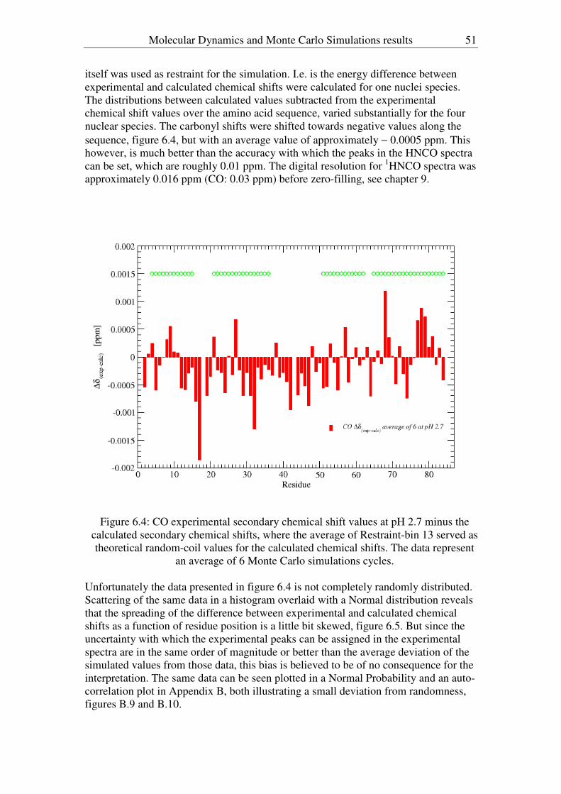
Molecular Dynamics and Monte Carlo Simulations results 51
itself was used as restraint for the simulation. I.e. is the energy difference between
experimental and calculated chemical shifts were calculated for one nuclei species.
The distributions between calculated values subtracted from the experimental
chemical shift values over the amino acid sequence, varied substantially for the four
nuclear species. The carbonyl shifts were shifted towards negative values along the
sequence, figure 6.4, but with an average value of approximately − 0.0005 ppm. This
however, is much better than the accuracy with which the peaks in the HNCO spectra
can be set, which are roughly 0.01 ppm. The digital resolution for 1HNCO spectra was
approximately 0.016 ppm (CO: 0.03 ppm) before zero-filling, see chapter 9.
Figure 6.4: CO experimental secondary chemical shift values at pH 2.7 minus the
calculated secondary chemical shifts, where the average of Restraint-bin 13 served as
theoretical random-coil values for the calculated chemical shifts. The data represent
an average of 6 Monte Carlo simulations cycles.
Unfortunately the data presented in figure 6.4 is not completely randomly distributed.
Scattering of the same data in a histogram overlaid with a Normal distribution reveals
that the spreading of the difference between experimental and calculated chemical
shifts as a function of residue position is a little bit skewed, figure 6.5. But since the
uncertainty with which the experimental peaks can be assigned in the experimental
spectra are in the same order of magnitude or better than the average deviation of the
simulated values from those data, this bias is believed to be of no consequence for the
interpretation. The same data can be seen plotted in a Normal Probability and an auto-
correlation plot in Appendix B, both illustrating a small deviation from randomness,
figures B.9 and B.10.

52 Molecular Dynamics and Monte Carlo Simulations results
Figure 6.5: Histogram of CO ∆δ(exp-calc) data for pH 2.7, average over 6 Monte Carlo
simulation cycles.
The amide nitrogen chemical shifts used as restraint in the MC-simulation had
significantly larger differences than both Cα and CO between experimental and
calculated chemical shifts values and were in the order of 0.1 ppm (see Figure B.11 in
Appendix B). Furthermore, those simulations also exhibited an odd distribution
between the different Restraint-bins, containing mostly structures from Restraint-bins
4, 5 and 6.
The deviation was not as large for the amide hydrogen chemical shifts, approximately
− 0.05 ppm, but all residues were equally affected and the distribution was odd as
well, with contributions mostly from Restraint-bin 6 and almost non from the random
coil Restraint-bin (the distribution can be seen in figure B.12 of Appendix B). Due to
these discrepancies and the nature of the experimental results for the HN and N
H
chemical shifts, it was decided that it was not worth pursuing these chemical shifts as
restraints any further.
Cα chemical shifts had overall deviations between the experimental and calculated
secondary chemical shifts of just around 0.0005 ppm, figure 6.6, which is an
extremely good agreement compared to the certainty with which the Cα peaks can be
assigned in the experimental spectra (HNCA), which is roughly 0.05 ppm. The
agreement between the experimental and simulated data is much better, than it is
possible to assign the peaks in the experimental spectra. The digital resolution for 1HNCA spectra was approximately 0.016 ppm (C
α: 0.07 ppm) before zero-filling, see
chapter 9. Therefore, once again, the fact that the differences along the amino acid
sequence are not randomly distributed is ignored. Figure 6.7 shows the Normal
probability plot for the data of figure 6.6, which in case of a random distribution
should be evenly distributed around the straight line and exhibit no deflection at the
end. Although not random, the deviation from a random distribution is very small.
Figures B.13 in Appendix B shows the scattering of the same data in a histogram
overlaid with a Normal distribution, while figure B.14 shows an autocorrelation plot.

Molecular Dynamics and Monte Carlo Simulations results 53
Figure 6.6: C
α experimental secondary chemical shift values at pH 2.7 subtracted
from the calculated secondary chemical shifts. The data represent an average of 8
Monte Carlo simulation cycles.
Simulations were also made where both Cα and CO chemical shifts served as
restraints. For these simulations the ensemble size was, exceptionally, chosen to
encompass only 1000 structures due to the lengthiness of these simulations.
Beforehand a simulation with an ensemble size of 10000 structures was run, and
compared to a simulation containing only an ensemble size 1000 structures. This
comparison revealed no major differences, neither for the secondary chemical shift
values, nor for the ensemble distribution between the different Restraint-bins. Those
simulations yielded also good correlations between experimental and calculated
values in the order of 0.005 ppm for carbonyl shifts and 0.03 ppm for Cα
shifts, figure
6.8. Strangely, the correlation for Cα shifts is not as good as it was for the simulations
where the Cα chemical shifts were used as sole restraint. However, the distribution of
the secondary chemical shifts (experimental minus calculated) for each residue
remains similar to the ones observed in simulations with just one chemical shift used
as restraint. The difference might indicate a difference in the information contained by
the two datasets.

54 Molecular Dynamics and Monte Carlo Simulations results
Figure 6.7: Normal Probability Plot for C
α ∆δ(exp-calc) pH 2.7, average of 8 Monte
Carlo simulation cycles.
Figure 6.8: C
α (red) and CO (blue) experimental secondary chemical shift values at
pH 2.7 subtracted from the calculated secondary chemical shifts. The data represent
an average over 6 Monte Carlo simulation cycles where both Cα and CO chemicals
shifts were used as restraints and made for simulations with an ensemble size of 1000
structures.

Molecular Dynamics and Monte Carlo Simulations results 55
Looking at the distributions of the calculated ensembles between the different
Restraint-bins, it was seen that regardless of which chemical shift was used as
restraint for the Monte Carlo simulations, they are all approximately the same, figures
6.9a-9c.
Figure 6.9a: Distribution for the ensembles found during MC-simulation, where C
α
chemical shifts at pH 2.7 were used as restraint, between the different Restraint-
bins of table 6.1. The number of structures in each Restraint-bin are out of a total of
10.000 possible structures for each Monte Carlo simulation cycle.
The MC-simulations minimize the energy between experimental and calculated
chemical shifts values for an ensemble of 10.000 structures, were the start ensemble
of 140.000 calculated structures served as a sampling pool. Among the 140.000
structures sub-ensembles with characteristics explained in table 6.1 exist. The original
MD-simulations of the Restraint-bins had a probability for α-helix of just about 30 %,
except for Restraint-bin 13, but the structures extracted from each Restraint-bin can
represent a larger or smaller propensity.
From figure 6.9a it is seen that the final distribution contained roughly [12.5-13 %] of
structures from Restraint-bin 1, [11-11.5%] from Restraint-bin 4, [9.5-10.5%] from
Restraint-bin 5, [10-11%] from Restraint-bin 8, [10.5-11%] from Restraint-bin 10,
[17-18%] from Restraint-bin 13 and [15-16%] from Restraint-bin 14. The remaining
Restraint-bins contain less than 2-3 %. In other words the resulting ensemble contains
approximately [40%] helix A4 at pH 2.7, while structures with helix A2 are
represented at [27%]. Helix A1 and A3 are almost evenly represented with roughly

56 Molecular Dynamics and Monte Carlo Simulations results
[10%] and [13%] respectively. It is also noted that the amount of random coil is
roughly [18%].
Figure 6.9b: Distribution between the different Restraint-bins, see table 6.1, of the
ensembles found during MC-simulation, where CO chemical shifts were used as
restraint at pH 2.7. The number of structures are out of a total of 10.000 possible
structures for each Monte Carlo simulation cycle.
If CO chemical shifts were used as sole restraint in the Monte Carlo simulations, the
distribution between the different Restraint-bins was roughly the same, figure 6.9b.
Here A4 could be accredited about [40%] of the time present in the ensemble, while
A2 accounted for [21%], A3 and A1 both for roughly [9.7%]. Notably the random
coil was represented with approximately 22 %, i.e. a few present more than if Cα was
used as a restraint. Another difference between the two simulations is that helix A2
exists to a lesser extent in this latest simulation, i.e. 21 % versus 27 %. So somehow
something different is modelled or measured by the MC-simulation with the two
restraints. For the Monte Carlo simulations where both Cα and CO were used as
restraint, figure 6.9c, the picture is similar, but with minor differences. The
distributions being spaced as followed; A4: [40%], A2: [24%], A3: [10%], A1: [7%]
and random-coil [22%]. This seems to be a distribution that resembles features of both
previous simulations; A4’s occupation equals the simulation where Cα was used as
restraint, while the amount of random-coil is similar to that seen for simulations
where CO chemical shifts were used as restraints.

Molecular Dynamics and Monte Carlo Simulations results 57
Figure 6.9c: Distribution between the different Restraint-bins, see table 6.1, of the
ensembles found during MC-simulation where both Cα + CO chemical shifts were
used as restraint. The number of structures are out of a total of 1.000 possible
structures for each Monte Carlo simulation cycle.
The question is, if the structures extracted out of each Restraint-bin in the different
Monte Carlo simulations represent the same amount of secondary structure. To check
the absolute distribution of the final ensembles, the secondary structure contents of
each Restraint-bin of the final ensembles were estimated with the program DSSPcont
[CAnder02]. This was done for all ensembles found for the repeated MC-simulations,
that is on approximately 60000 – 80000 structures. Figures 6.10 to 6.11 are examples
of the different secondary structure contents under the different simulation conditions
(Cα, CO and C
α + CO used as restraints in the MC-simulations) for certain of the
Restraint-bins.
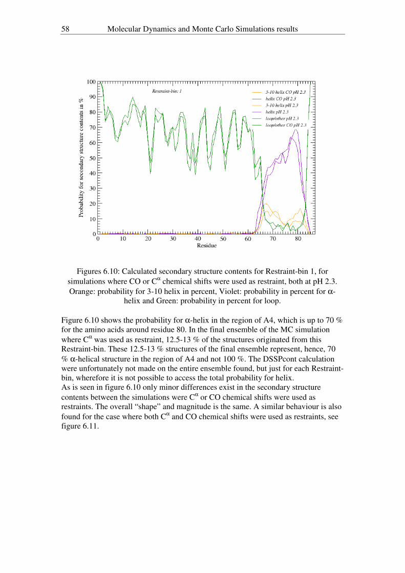
58 Molecular Dynamics and Monte Carlo Simulations results
Figures 6.10: Calculated secondary structure contents for Restraint-bin 1, for
simulations where CO or Cα chemical shifts were used as restraint, both at pH 2.3.
Orange: probability for 3-10 helix in percent, Violet: probability in percent for α-
helix and Green: probability in percent for loop.
Figure 6.10 shows the probability for α-helix in the region of A4, which is up to 70 %
for the amino acids around residue 80. In the final ensemble of the MC simulation
where Cα was used as restraint, 12.5-13 % of the structures originated from this
Restraint-bin. These 12.5-13 % structures of the final ensemble represent, hence, 70
% α-helical structure in the region of A4 and not 100 %. The DSSPcont calculation
were unfortunately not made on the entire ensemble found, but just for each Restraint-
bin, wherefore it is not possible to access the total probability for helix.
As is seen in figure 6.10 only minor differences exist in the secondary structure
contents between the simulations were Cα or CO chemical shifts were used as
restraints. The overall “shape” and magnitude is the same. A similar behaviour is also
found for the case where both Cα and CO chemical shifts were used as restraints, see
figure 6.11.

Molecular Dynamics and Monte Carlo Simulations results 59
Figures 6.11: Calculated secondary structure contents for Restraint-bin 14 in percent,
for simulations where Cα or (C
α + CO) chemical shifts were used as restraint, both at
pH 2.7. Orange: probability for 3-10 helix, Blue: probability for α-helix and Green:
probability for loop.
6.2.2 Monte Carlo simulations of pH 2.3
The pH-titration experiments were performed to get quantitative information about
the helical contents during the folding process using experimental chemical shifts.
More so, if it was possible to get absolute differences in the tendency for helix
formation between the distinct pH values. Therefore the Monte-Carlo simulations also
included modelling of the experimental data obtained at pH 2.3. Here only
simulations with Cα or carbonyl chemical shifts as restraint were performed and the
results can be seen in figures 6.12 and 6.13.

60 Molecular Dynamics and Monte Carlo Simulations results
Figure 6.12: C
α experimental secondary chemical shift values at pH 2.3 subtracted
from the calculated secondary chemical shifts. The data represent an average of 6
Monte Carlo simulation cycles. The red circles denote the location of the four α-
helices in the native structure of ACBP.
The distribution of secondary chemical shift differences seems to be similar to the one
obtained at pH 2.7: Both in overall magnitude and the areas that are distributed away
from randomness, i.e. the second half of peptide segment comprising helix A1 of the
native structure and the first loop, as well as in the middle of the large loop, figure
6.12. Also the differences for carbonyl shifts are comparable to those found at pH 2.7,
and are again defined better than the experimental uncertainty for assignment of the
peaks in the experimental spectra, figure 6.13.

Molecular Dynamics and Monte Carlo Simulations results 61
Figure 6.13: CO experimental secondary chemical shift values at pH 2.3 subtracted
from the calculated secondary chemical shifts. As before, the calculated secondary
chemical shifts were found by subtracting the average of Restraint-bin 13, which
served as theoretical random-coil values. The data represent an average of 6 Monte
Carlo simulations cycles. The red circles denote the location of the four α-helices in
the native structure of ACBP.
As seen from figures 6.14 the distribution between the different Restraint-bins is very
similar to that seen at pH 2.7. However, it is clearly seen that the amount of helical
secondary structure is significantly reduced and the amount of random coil drastically
increased by almost 6.5 %. At pH 2.3 the percentage of structures containing A4
helical propensity is reduced by 5.5 % compared to pH 2.7. A2 is not reduced as
radically, and merely accounts for a loss of 1.6 %. A3 and A1 fall by roughly 2 and 3
percent, respectively.
Contrary to this clear behaviour the distribution between the Restraint-bins for MC-
simulations were CO chemical shifts served as restraint do not change at all, figure
6.15. At this lower pH the distribution still is A4 ~ 40 %, A2 ~ 21 %, A3 and A4 still
both 9.7%, and Restraint-bin 13 22 %. The overall distributions from all Monte Carlo
simulations are summarized in table 6.2.

62 Molecular Dynamics and Monte Carlo Simulations results
Figure 6.14: Distribution between the different Restraint-bins, see table 6.1, of the
ensembles found during MC-simulations, where Cα was used as restraint at pH 2.3.
The number of structures in each Restraint-bin are out of a total of 10.000 possible
structures for each Monte Carlo simulation cycle.
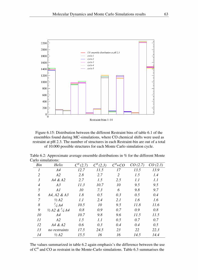
Molecular Dynamics and Monte Carlo Simulations results 63
Figure 6.15: Distribution between the different Restraint bins of table 6.1 of the
ensembles found during MC-simulations, where CO chemical shifts were used as
restraint at pH 2.3. The number of structures in each Restraint-bin are out of a total
of 10.000 possible structures for each Monte Carlo simulation cycle.
Table 6.2: Approximate average ensemble distributions in % for the different Monte
Carlo simulations:
Bin Helix Cα (2.7) C
α (2.3) C
α+CO CO (2.7) CO (2.3)
1 A4 12.7 11.5 17 13.5 13.9
2 A2 2.8 2.7 2 1.5 1.4
3 A4 & A2 2.7 1.5 2.5 1.1 1.1
4 A3 11.3 10.7 10 9.5 9.5
5 A1 10 7.3 6 9.8 9.7
6 A4, A2 & A3 1.8 0.5 0.3 0.5 0.4
7 ½ A2 1.1 2.4 2.1 1.6 1.6
8 3⁄4 A4 10.5 10 9.5 11.8 11.6
9 ½ A2 & 3⁄4 A4 0.8 0.9 0.7 0.9 0.8
10 A4 10.7 9.8 9.6 11.5 11.5
11 A2 1.5 1.1 0.5 0.7 0.7
12 A4 & A2 0.6 0.3 0.4 0.4 0.5
13 no restraints 17.5 24.5 23 22 22.3
14 ½ A2 15.5 16 16 14.5 14.4
The values summarized in table 6.2 again emphasis’s the difference between the use
of Cα and CO as restraint in the Monte-Carlo simulations. Table 6.3 summarises the

64 Molecular Dynamics and Monte Carlo Simulations results
approximate total distributions between the four helical regions from the different
Monte Carlo simulations.
Table 6.3: Approximate average ensemble distributions between the different helical
regions for the different Monte Carlo simulations:
Helix Cα (2.7) C
α (2.3) C
α+CO CO (2.7) CO (2.3)
A1 10 % 7 % 7 % 10 % 10 %
A2 27 % 25 % 24 % 21 % 21 %
A3 13 % 11 % 10 % 10 % 10 %
A4 40 % 34.5 % 40 % 40 % 40 %
Figure 6.16 illustrates the loss of helix propensity in the structures of Restraint-bin 4,
where it is seen that α-helix probability in the area of helix A3 in the native protein
goes down from 50 % to 46 % when the pH is lowered from 2.7 to 2.3. Again, this is
only the probability for α-helical contents of helix A3 in 10 % and 11 % of the
structures found during the MC simulations with Cα used as restraint at pH 2.3 and
pH 2.7.
Figures 6.16: Calculated secondary structure contents for Restraint-bin 4 in percent,
for simulations where Cα was used as restraint, both at pH 2.3 and pH 2.7.
Orange/red: probability for 3-10 helix, Blue/violet: probability for α-helix and
Light/green: probability for loop.

Molecular Dynamics and Monte Carlo Simulations results 65
If one examines the probabilities for secondary structure contents as calculated by
DSSPcont for all structures found during one Monte Carlo simulation, i.e. 10.000
structures, it is seen that the overall probability for α-helix in the region A4 is just
below 20 %, figure 6.17. The region of helix A2 in the native structure of ACBP
exhibits less than 10 % α-helix and the regions A3 and A1 represent even less. The
probability for 3-10 helix in the region A4 is by DSSPcont estimated to be around 6
%, therefore the overall probability for helix is roughly 25 % for the 10.000 structures
found in one MC-simulation at pH 2.3. In contrast, just below 35% of the structures
originated from Restraint-bins where this region was restrained, see table 6.3.
Figures 6.17: Calculated secondary structure contents in percent for all structures
found in one MC-simulation, i.e. 10.000, where Cα was used as restraint at pH 2.3.
Blue: probability for 3-10 helix, Red: probability for α-helix, Green: probability for
loop/other.
Ideally, the ensemble found in Monte-Carlo simulations, with one chemical shift
species as restraint, should be able to predict the chemical shift pattern for the other
shift not used as restraint. Unfortunately, the ensemble for one run yields an
absolutely different pattern for the chemical shift not used as restrained. For instant, a
run with Cα as restraint yields differences between experimental and calculated
chemical shift values for CO of approximately − 0.3 ppm and up to – 0.8 ppm and a
pattern different from the one observed in a MC-simulation. A graphical
representation can be found in Appendix B, figure B.15.
6.3 PALES

66 Molecular Dynamics and Monte Carlo Simulations results
The ensemble found in the Monte-Carlo simulations, with one chemical shift species
as restraint, should be able to predict the chemical shift pattern for the other shift not
used as restraint. Unfortunately, this was not the case, but in order to validate the
predictive power of the ensembles found, they were used with the program PALES
[MZweck00]. PALES calculates/predicts residual dipolar couplings (RDC) from pdb-
files. That is, it predicts sterically induced alignment in dilute liquid crystalline phase.
These were compared to RDCs found for ACBP at pH 2.3 by W. Fieber et al.
[WFiebe04]. For each structure found in the ensembles manufactured during a Monte
Carlo simulation dipolar couplings were predicted by PALES and subsequently the
average of all structures was calculated. PALES needs an initial set of dipolar
couplings and here the experimental values at pH 2.3 [WFiebe04] were used. For the
prediction of residual dipolar coupling default simulation parameters where used.
That is the orientation is simulated by an infinite wall and a standard concentration of
liquid crystal. Each set of dipolar couplings were scaled by -4 in order to somewhat
accommodate the alignment media used. Shortle and Ackerman [DShortle01] note
that compression versus stretching yield dipolar couplings of opposite sign. Mohana-
Borges et al. [RMohan04] additionally note a factor 2 between the two types. It is not
expected that PALES is able to predict the exact size of the dipolar couplings, and
scaling always has to be applied [AAlmon02]. In Figure 6.18 N-H experimental
dipolar couplings for ACBP at pH 2.3 are seen together with predicted dipolar
couplings calculated on the basis of Monte Carlo simulations were Cα or CO chemical
shifts were used as restraints at pH 2.3. That is, the predicted dipolar couplings in
each case represent an average over 60.000 structures. The overall magnitude of the
individual N-H dipolar couplings are as expected not predicted very well on the basis
of the two ensembles found in the MC-simulations. However, the overall pattern,
particularly in the region of helix A4 in the native structure, is represented by both
ensembles. Most couplings are negative and get smaller in magnitude or positive in
areas were the observed couplings behaviour is similar, e.g. the first half of the region
A2 and the loop region between helix A2 and A3 of the native structure. This is a very
encouraging result supporting the validity of the ensembles found in the MC-
simulations.
Figure 6.19 shows the correlation between experimental and calculated dipolar
couplings of the two ensembles. The correlation coefficient lies between 0.4 and 0.44
for the predictions on the basis of the “CO-ensemble” and “Cα-ensemble”,
respectively. That is the covariance is roughly 20 %.

Molecular Dynamics and Monte Carlo Simulations results 67
Figure 6.18: a) Experimental N-H dipolar coupling of ACBP at pH 2.3 as a function
of residue position. The dipolar couplings were taken from [WFiebe04]. b) Predicted
N-H dipolar couplings on the basis of the ensembles found in MC-simulations with
Cα chemical shifts as restraints. c) Predicted N-H dipolar couplings on the basis of
the ensembles found in MC-simulations with CO chemical shifts as restraints. The
red circles represent the position of the four α-helices in the native structure of
ACBP.
The relative small correlations originate from the inability to exactly model the
dipolar couplings for each specific residue. The important point, however, is the
ability to reproduce the overall features like the positive dipolar couplings of region
A4. Another possibility for the small covariance might be that the observed RDCs
sample a different ensemble than chemical shifts. RDCs measure the fractions of
molecules that are restricted due to the alignment media, whereas chemical shifts
represent an average of all molecules [AAlmon02].

68 Molecular Dynamics and Monte Carlo Simulations results
Figure 6.19: Correlation between predicted
1DNH values and experimentally
observed [WFiebe04]. The two predicted ensembles are those found during MC-
simulations at pH 2.3, where CO and Cα chemical shifts were used as restraints.
6.4 Discussion/Conclusion
In order to evaluate the chemical shift data obtained in the acid denaturing titration
series, Molecular Dynamic and Monte Carlo simulations where performed. It seems
that it is possible to reproduce the experimental features, obtained for the unfolding of
ACBP, by comparing the experimental chemical shift data to those found theoretically
by SHIFTX. It was hence possible to obtain ensembles of conformations that
represent the denatured state of ACBP at two pH values. It was consequently
observed that the amount of structures with helical propensity decrease by around 7 %
from pH 2.7 to pH 2.3. Noticeable, the largest loss of tendency for helix formation
was found for the area that is helix A1 in the native protein. But also an increase in
helix propensity from pH 2.7 to 2.3 in the second half of helix A2 was observed and
signified a very peculiar behaviour, table 6.2 (bin 7). According to these computer
simulations ACBP still contains a considerable amount of secondary helical structure
at pH 2.3. The largest tendency for helix is found for the area of helix A4 in the native
protein, which still accounts for roughly 34 %, followed by A2 with 25 %, A3 with 11
% and A1 with 7 %. Those ensembles, however, signify not a 100 % probability for
helix, but just a percentage. For example, as was seen in figure 6.16, the combined
probability for 3-10 and α-helix in the area of helix A3 of the native structure is
roughly 60 % at pH 2.3. This should be seen in relation to the original MD-
simulations of Restraint-bin 4, which had a probability for α-helix of just about 30 %.
Therefore it is possible to find ensembles, which depict the experimentally found
observation that the helix propensity for ACBP slowly decreases over the pH titration

Molecular Dynamics and Monte Carlo Simulations results 69
range and residual secondary structure still exists at pH 2.3. These results fit very well
with previous experimental results obtained for ACBP. As mentioned in chapter 2,
these experiments suggest the early formation of helical structure in A4, which was
derived from the observation that the amide hydrogens were protected against
exchange. Subsequently long-range interactions are formed between A1, A2 and A4
in the transition state, where A2 and A4 interact and stabilize each other, the two
helices, which have the highest propensity for helix in this study.
The simulations were nevertheless ambiguous, in a sense that the energy minimisation
against carbonyl carbon chemical shifts did not behave as those made with Cα
chemical shifts. Those ensembles did not reveal a change in helix propensities from
pH 2.7 to pH 2.3, and also represented a slightly different percentile distribution of
A2, A3, A4 and random-coil values than those found for Cα chemical shifts. As a
consequence of this the ensembles obtained by using one chemical shift as restraint in
the Monte Carlo simulation could not be used to predict the behaviour of the other
chemical shift. This lack of cross-validation is of course problematic. It might arise
from the different uncertainties by which the different chemical shifts are theoretically
determined. SHFTX used empirically derived chemical shift hypersurfaces in
combination with classical or semi-classical equations, that relatively accurate
describe their effects, to calculate the chemical shifts from atomic coordinates
[SNeal03]. The purpose of the hypersurfaces was to encapsulate effects, like nearest
neighbour, dihedral angles and secondary structure, which are problematic to describe
analytically and are calculated on the basis of a database of observed chemical shifts.
Generally the correlation and RMS error for 13
Cα was better than that for
13CO, which
might explain the inability of the MC simulation with CO as restraint to capture the
subtle differences between the different pH values. If one compares the correlation
coefficients for calculated chemicals shifts found by S. Neal et al. [SNeal03] for the
different carbons solely determined by physical factors (classical equations) and
together with hypersurfaces, a big difference is noted. It is such that correlations
factors are significantly improved for carbonyl carbon when empirical hypersurfaces
are included (∆ 0.35), whereas the predictive power for Cα just is slightly increased (∆
0.08). The hypersurfaces are constructed for folded proteins, that is the data-bases
were trained against well-structured proteins of different structural classes and one
could imaging that exactly the ability of the hypersurface to capture effects of
statistical nature like secondary structure might be the nature of this difference. And
since we look at a denatured protein the correlation coefficient for CO by SHIFTX
might actually be much poorer than assumed.
Generally it should be noted that the found ensembles only represent the right
conformational distributions of the experiment if the right structures are part of the
original start ensemble. This is a big disadvantage of an else wise very simple
approach that is easily implemented. After construction of the initial start ensemble it
is not possible to add structures during a run, forcing one to manually define
structures by restraining their dihedral angles and running the risk of omitting
structures and guessing wrong. The small deviations between experimental and
calculated chemical shifts are, however, very encouraging.
The N-H dipolar couplings predicted by PALES on the basis of the ensembles found
during the Monte Carlo simulations fit relatively well with observed dipolar couplings
for ACBP at pH 2.3. The ability of the chemical shift data to predict the observed
pattern of dipolar couplings, via computational approaches, yields a self-consistent
representation and supports the validity of the ensembles found during the Monte
Carlo simulations. To my knowledge the obtained data are both novel and powerful.

70 Molecular Dynamics and Monte Carlo Simulations results
The achievement is a very accurate estimate of helix formation in the acid unfolded
state and a precise tracking of the loss of residual secondary structure over a pH
interval.
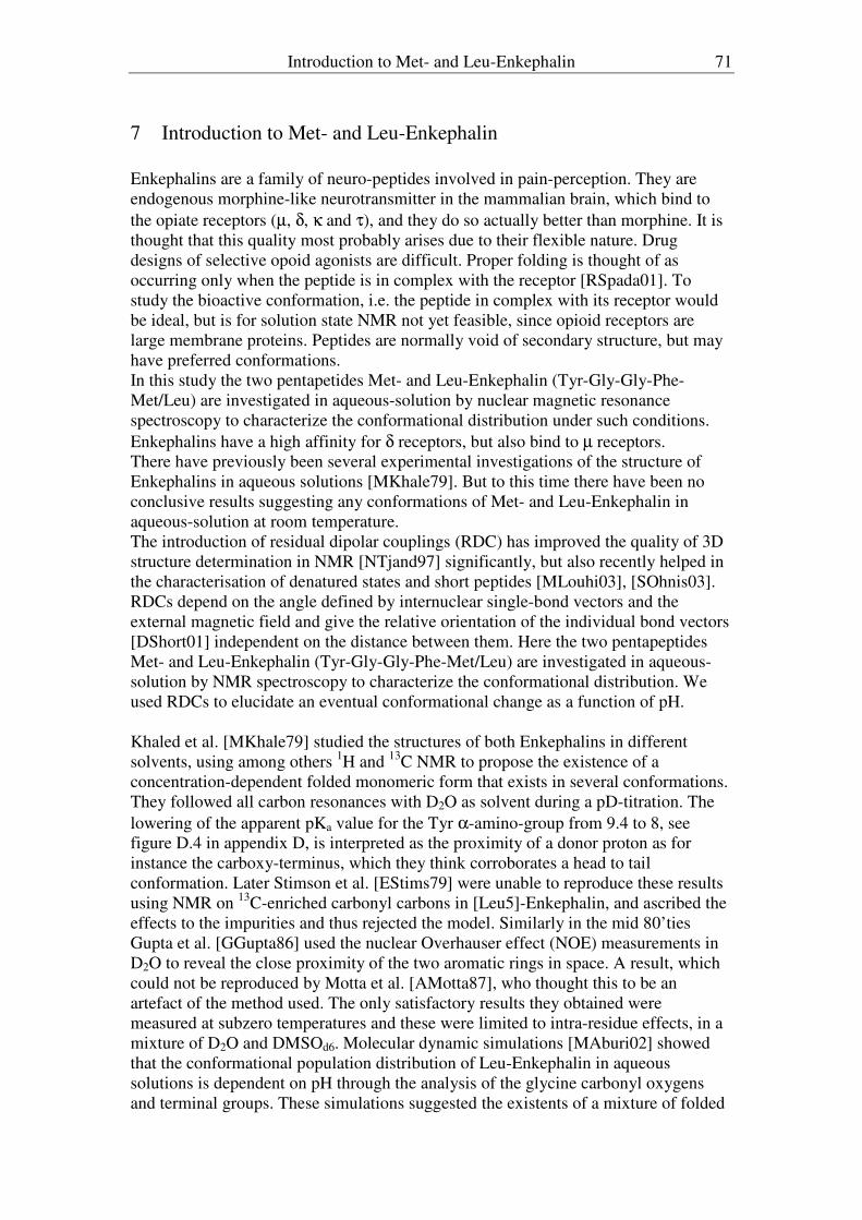
Introduction to Met- and Leu-Enkephalin 71
7 Introduction to Met- and Leu-Enkephalin
Enkephalins are a family of neuro-peptides involved in pain-perception. They are
endogenous morphine-like neurotransmitter in the mammalian brain, which bind to
the opiate receptors (µ, δ, κ and τ), and they do so actually better than morphine. It is
thought that this quality most probably arises due to their flexible nature. Drug
designs of selective opoid agonists are difficult. Proper folding is thought of as
occurring only when the peptide is in complex with the receptor [RSpada01]. To
study the bioactive conformation, i.e. the peptide in complex with its receptor would
be ideal, but is for solution state NMR not yet feasible, since opioid receptors are
large membrane proteins. Peptides are normally void of secondary structure, but may
have preferred conformations.
In this study the two pentapetides Met- and Leu-Enkephalin (Tyr-Gly-Gly-Phe-
Met/Leu) are investigated in aqueous-solution by nuclear magnetic resonance
spectroscopy to characterize the conformational distribution under such conditions.
Enkephalins have a high affinity for δ receptors, but also bind to µ receptors.
There have previously been several experimental investigations of the structure of
Enkephalins in aqueous solutions [MKhale79]. But to this time there have been no
conclusive results suggesting any conformations of Met- and Leu-Enkephalin in
aqueous-solution at room temperature.
The introduction of residual dipolar couplings (RDC) has improved the quality of 3D
structure determination in NMR [NTjand97] significantly, but also recently helped in
the characterisation of denatured states and short peptides [MLouhi03], [SOhnis03].
RDCs depend on the angle defined by internuclear single-bond vectors and the
external magnetic field and give the relative orientation of the individual bond vectors
[DShort01] independent on the distance between them. Here the two pentapeptides
Met- and Leu-Enkephalin (Tyr-Gly-Gly-Phe-Met/Leu) are investigated in aqueous-
solution by NMR spectroscopy to characterize the conformational distribution. We
used RDCs to elucidate an eventual conformational change as a function of pH.
Khaled et al. [MKhale79] studied the structures of both Enkephalins in different
solvents, using among others 1H and
13C NMR to propose the existence of a
concentration-dependent folded monomeric form that exists in several conformations.
They followed all carbon resonances with D2O as solvent during a pD-titration. The
lowering of the apparent pKa value for the Tyr α-amino-group from 9.4 to 8, see
figure D.4 in appendix D, is interpreted as the proximity of a donor proton as for
instance the carboxy-terminus, which they think corroborates a head to tail
conformation. Later Stimson et al. [EStims79] were unable to reproduce these results
using NMR on 13
C-enriched carbonyl carbons in [Leu5]-Enkephalin, and ascribed the
effects to the impurities and thus rejected the model. Similarly in the mid 80’ties
Gupta et al. [GGupta86] used the nuclear Overhauser effect (NOE) measurements in
D2O to reveal the close proximity of the two aromatic rings in space. A result, which
could not be reproduced by Motta et al. [AMotta87], who thought this to be an
artefact of the method used. The only satisfactory results they obtained were
measured at subzero temperatures and these were limited to intra-residue effects, in a
mixture of D2O and DMSOd6. Molecular dynamic simulations [MAburi02] showed
that the conformational population distribution of Leu-Enkephalin in aqueous
solutions is dependent on pH through the analysis of the glycine carbonyl oxygens
and terminal groups. These simulations suggested the existents of a mixture of folded
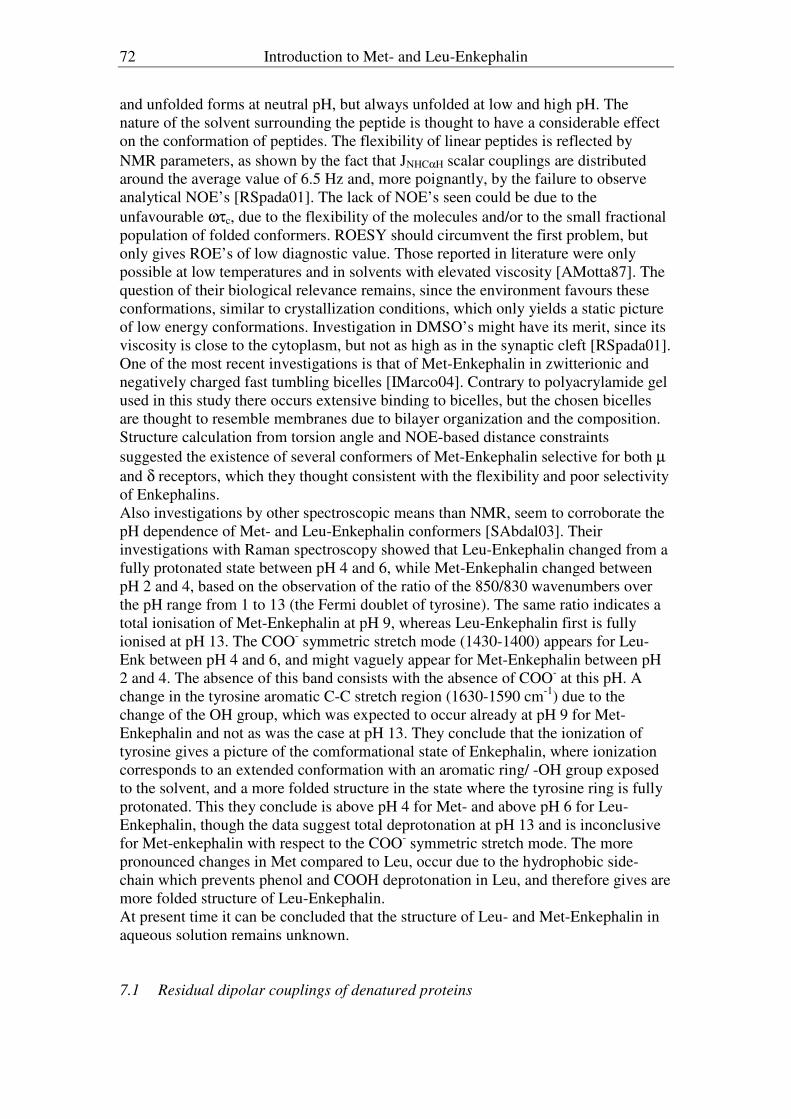
72 Introduction to Met- and Leu-Enkephalin
and unfolded forms at neutral pH, but always unfolded at low and high pH. The
nature of the solvent surrounding the peptide is thought to have a considerable effect
on the conformation of peptides. The flexibility of linear peptides is reflected by
NMR parameters, as shown by the fact that JNHCαH scalar couplings are distributed
around the average value of 6.5 Hz and, more poignantly, by the failure to observe
analytical NOE’s [RSpada01]. The lack of NOE’s seen could be due to the
unfavourable ωτc, due to the flexibility of the molecules and/or to the small fractional
population of folded conformers. ROESY should circumvent the first problem, but
only gives ROE’s of low diagnostic value. Those reported in literature were only
possible at low temperatures and in solvents with elevated viscosity [AMotta87]. The
question of their biological relevance remains, since the environment favours these
conformations, similar to crystallization conditions, which only yields a static picture
of low energy conformations. Investigation in DMSO’s might have its merit, since its
viscosity is close to the cytoplasm, but not as high as in the synaptic cleft [RSpada01].
One of the most recent investigations is that of Met-Enkephalin in zwitterionic and
negatively charged fast tumbling bicelles [IMarco04]. Contrary to polyacrylamide gel
used in this study there occurs extensive binding to bicelles, but the chosen bicelles
are thought to resemble membranes due to bilayer organization and the composition.
Structure calculation from torsion angle and NOE-based distance constraints
suggested the existence of several conformers of Met-Enkephalin selective for both µ
and δ receptors, which they thought consistent with the flexibility and poor selectivity
of Enkephalins.
Also investigations by other spectroscopic means than NMR, seem to corroborate the
pH dependence of Met- and Leu-Enkephalin conformers [SAbdal03]. Their
investigations with Raman spectroscopy showed that Leu-Enkephalin changed from a
fully protonated state between pH 4 and 6, while Met-Enkephalin changed between
pH 2 and 4, based on the observation of the ratio of the 850/830 wavenumbers over
the pH range from 1 to 13 (the Fermi doublet of tyrosine). The same ratio indicates a
total ionisation of Met-Enkephalin at pH 9, whereas Leu-Enkephalin first is fully
ionised at pH 13. The COO- symmetric stretch mode (1430-1400) appears for Leu-
Enk between pH 4 and 6, and might vaguely appear for Met-Enkephalin between pH
2 and 4. The absence of this band consists with the absence of COO- at this pH. A
change in the tyrosine aromatic C-C stretch region (1630-1590 cm-1
) due to the
change of the OH group, which was expected to occur already at pH 9 for Met-
Enkephalin and not as was the case at pH 13. They conclude that the ionization of
tyrosine gives a picture of the comformational state of Enkephalin, where ionization
corresponds to an extended conformation with an aromatic ring/ -OH group exposed
to the solvent, and a more folded structure in the state where the tyrosine ring is fully
protonated. This they conclude is above pH 4 for Met- and above pH 6 for Leu-
Enkephalin, though the data suggest total deprotonation at pH 13 and is inconclusive
for Met-enkephalin with respect to the COO- symmetric stretch mode. The more
pronounced changes in Met compared to Leu, occur due to the hydrophobic side-
chain which prevents phenol and COOH deprotonation in Leu, and therefore gives are
more folded structure of Leu-Enkephalin.
At present time it can be concluded that the structure of Leu- and Met-Enkephalin in
aqueous solution remains unknown.
7.1 Residual dipolar couplings of denatured proteins

Introduction to Met- and Leu-Enkephalin 73
Residual dipolar couplings (RDC) have been used to significantly improved structure
determination in NMR [NTjand97], but not until recently been implemented in the
characterisation of denatured states and short peptides [MLouhi03], [SOhnis03],
[AAlexa03]. Weak alignment of proteins prevents the complete averaging of dipolar
interactions, but preserve the solution properties of the sample. RDCs depend on the
angle defined by internuclear single-bond vectors and the external magnetic field and
give the relative orientation of the individual bondvectors [DShort01] independent on
the distance between them.
Dipolar couplings originate from the interaction between two magnetic dipoles. The
interaction energy between two point dipoles (µµµµ1 and µµµµ2) is given by:
⋅⋅⋅
−⋅
=Η5
21
3
2102
21
)ˆ()ˆ(3
ˆˆ
4ˆ
r
II
r
IIdd
rr
π
µγγ h
7.1
Where r is the distance between the dipoles and µµµµ = γ h/2π I. In solution NMR dipolar
couplings average to zero due to rapid isotropic tumbling. In acryl amide gel, bicelles
and other anisotopic nematic liquid crystalline media the tumbling is restricted by a
fraction in one direction, with is enough to ensure incomplete averaging and get
measurable residual dipolar couplings.
The magnitude of the RDC is dependent on the orientation of the internuclear vector
relative to the alignment tensor of the entire protein [RMohan04]. In other words,
bond vectors such as 15
N-1H or
13C-
1H can be oriented relative to a global alignment
tensor fixed in the molecular frame, independent of their location in the molecule.
This can be deduced from equation 7.1 giving that the relative orientations between
pairs of bond vectors are independent of the distance between them.
( ) ( )[ ]φθθπ
µγγ2cossin
231cos3
4
22
2
0
3 ra
NH
HN
NHAA
rSD +−−=
h
7.2
S is the generalized order parameter, γN, γH the gyromagnetic ratios and Aa, and Ar are
the axial and rhombic components of the alignment tensor.
It was previously implicitly assumed that the RDCs of a fully denatured protein would
be zero. But studies have shown that even under strong denaturing conditions proteins
can be aligned and dipolar couplings [DShort01] of similar composition as in the
native state observed. Screening of short peptides from 2 to 15 amino acids in length
revealed small RDCs for the peptides aligned in both bicelles or polyacrylamide gels
[SOhnis03], inferring a non-spherical conformational ensemble. Line-broadening in
the bicelles, but not in acrylamide gel, suggested the alignment here arose due to
peptide binding, whereas steric hindrance was thought to be the only mechanism
responsible for alignment in acryl-amide gels. The arbitrary composition of the
studied peptides, except for low fraction of hydrophobic residues, reflects the intrinsic
structural properties of small peptides, leading to the view of the denatured state of a
protein to be composed of stiff segments with strong directional bias.
The assumption that residual dipolar couplings average to zero in denatured proteins
and short peptides ignores the classical results of “random flight chain” of Kuhn

74 Introduction to Met- and Leu-Enkephalin
according to Louhivuori et al. [MLouhi03]. In 1934 in Kolloid-Z [MLouhi03a] Kuhn
pointed out that segments of the random flight chain not are scattered spherically
relative to the end-to end displacement axis. Louhivuori et al. [MLouhi03] show how
this simple structure of the chain will cause nonvanishing RDCs by using the model
of the random flight chain (Gaussian chain). They assume for the spatial distribution
of an ensemble of conformers, that no conformational changes are induced by the
obstruction itself and calculate the average orientation of each segment. They find that
the probability of the internuclear vector with respect to the magnetic field for longer
chains will become smaller, since the distribution of uncorrelated chain segments will
go towards a more spherical one. This probability goes towards zero for the infinitely
long change and simulations of the chain length in bicelles reveal dipolar couplings of
the order of a few Hertz for short chains of length 10 to 100. They also observe that
the couplings go towards zero towards the chain termini and hence have a very
particular distribution along the peptide sequence.
Significant residual dipolar couplings have also been observed for both acid and urea
denatured apomyoglobin [RMohan04], where changes in RDCs are observed in local
regions with helical propensities in the acid-denatured state. Similar observations in
the acid-denatured state are made for ACBP, where also mutation of a single residue
in one helical area lead to large decreases of RDCs in a second helical area of the
native state [WFiebe04]. The behaviour of a chain can also be described in terms of
its persistence length [RMohan04]. The persistence length is a measure of the length
at which the chain continues in the same direction and has been measured for
denatured polypeptides to be five to seven amino acid residues long. The statistical
segment lengths is approximately double the persistence length, and each statistical
segment, with a propensity towards extended conformation, is highly anisotropic in
shape with its own alignment tensor. Mohana-Borges et al. further suggest that RDCs
in unstructured polypetides derive from transient alignment of these local regions of
the chain. That is, contrary to RDCs for folded globular proteins, RDCs in denatured
proteins and short peptide are not determined by the relative orientation of a bond
vector to a single global alignment tensor, but arise due alignment of statistical
segments or transient elements of secondary structure. Due to this local alignment
tensor, it might be inferred that small peptides in extended conformation aligned with
the obstructing plane have a larger contribution to the observed RDCs, as compared to
more bended structures aligned with an angle. Therefore RDC measurement on
denatured proteins and peptides give information on the composition of a
conformational ensemble, and may for example be used for comparison with values
calculated for ensembles of conformations derived during molecular dynamic
simulations.

Results for Met and Leu-Enkephalin 75
8 Results for Met and Leu-Enkephalin
All resonances of Met- and Leu-Enkephalin were assigned on the basis of 13
CHSQC-, 15
NHSQC-, TOCSY- and HMBC- experiments. In the search for inter residual NOE’s
that could suggest a dominating conformation ROESY-, NOESY-pulse sequences
were applied, but were unsuccessful. Therefore our attention turned to residual dipolar
couplings (some NOESY measurements were made on 500 MHz Brucker Instruments
at Carlsberg Laboratories). The investigation were done below and above the
theoretical pI of 5.52 [Expasy], in 100 mM KCl and 10 % D2O at pH 2.0, 4.04, 6.95
and 8.9 and 2.0, 4.06 and 6.95 for unlabelled Met- and Leu-Enkephalin respectively,
all at T = 298K. The concentrations used for both peptides were typically from 6 mM
to 16 mM. The pH interval from pH 2 to 9 was chosen in order to investigate the
peptides in their cationic, zwitterionic and anionic states, since changes in the ionic
state of small peptides can represent large environmental changes. The residual
dipolar couplings were measured with gTOCSYNHSQC or IPAP-NHSQC on Varian
Unity Inova Instruments 750 MHz and 800 MHz spectrometers at T = 298K, and for
Leu-Enkephalin also encompassed in addition to the above mentioned pH-values: pH
1, 3, 5, 6 and 8.
8.1 NOESY
An attempt was made to obtain inter-residual NOE’s, which could suggest a
dominating conformation. Several intra-residual NOE’s and a few inter-residual
NOE’s between e.g. Gly-2 NH and Hα, and H
β of tyrosine, and between NH of the
glysines were observed. Never the less, none were observed between the sidechains.
The lack of inter-residual NOEs is most probably due to the flexibility of the
molecules, where the lifetime of individual conformations is too short to allow for
measurable NOE build-up. WROESY measurements with mixing times from 200 ms
to 400 ms were tried, and established, where NOE build up was not eaten by
exchange, to be best around 250 ms. The lack of inter-residual NOE’s could also be
due to a small fractional population of “folded” conformers (less than ~ 5%
populated) at any given time. Nevertheless, differences in the amide proton chemical
shifts at different pH-values were observed. The chemical shift of HN - of methionine
changes from 8.4 ppm at pH 2 to 8.06 at pH 4, i.e. a change of -0.37 ppm, whereas HN
of Phe-4, Gly-3 and Gly-2 change -0.022, +0.032 and +0.022 respectively, see figures
D.1 and D.2 in Appendix D. This most probably is due to the deprotonation of the C-
terminus. The fact that the effect is larger on Gly-3, which is further apart from the
deprotonation centre than Phe-4, insinuates additional influences on the chemical shift
changes other than deprotonation.
8.2 Residual dipolar couplings
This prompted the investigation of RDCs over the pH range from pH 1 to 9, in
stretched polyacrylamide gels, which are stable and inert over a broad range of
conditions (for instance low pH), contrary to bicelles and phages [RMohan04]. It has
been shown that alignment by strained polyacrylamide gels occurs due to steric
hindrance in proteins as well as in small peptides. Contrary hereto akyl-PEG-bicelles
seem additionally to mediate alignment through transient binding [SOhni03]. In these
experiments 7% w/v strained polyacrylamide gel, as described in chapter 9, were used

76 Results for Met and Leu-Enkephalin
[JChou01], [RTycko00], [HSass00]. This compression provided a deuterium
quadrupolar coupling of 12-16 Hz. Unfortunately, several of the labile protons
exchange beyond detection in the gel at relatively low pH. Glycine-2 exchanges
beyond detection already at pH 6, Gly-3 at pH 7 and Phe-4 at pH 8 leaving just one
residual dipolar coupling between 15
N and 1H
N of Leucine-5 at pH 8. In Appendix D
figure D.3 the theoretical calculated exchange rates for Leu-Enkephalin [YZhang],
which collaborate these results, are shown. There exist several methods for obtaining
RDCs by NMR. Natural abundance 15
N HSQC spectra were collected, without
decoupling during acquisition time, under isotropic (1JNH) and partially aligned (
1JNH
+ DNH) (anisotropic) conditions in order to obtain RDCs, with approximately 12 h of
data collection for TOCSY-NHSQC and IPAP-NHSQC spectra with roughly 6-8
hours of data collection [NTjand97]. The RDCs were calculated as the difference
between scalar couplings measured in the isotropic sample and total couplings in the
oriented sample [AAlexa03]. Yielding, (1JNH) - (
1JNH + DNH) = - DNH.
All spectra's were analysed using NMRView software, while an in-house program
(APK) was used to determine the scalar and dipolar couplings. No differences in
proton linewidths between aligned and isotropic samples were observed, it was
therefore interpreted that no binding to the alignment media occurred. We measured
the pH-dependence of RDCs for both Enkephalins at the pH values 2, 4, 7 and 9, at
pH 9, as explained above, all amide protons exchanged. For Leu-Enkephalin RDCs
were additionally obtained at pH 1, 3, 5, 6, and 8, as well as reproduced at pH 2 and 3
(that is also measured with the two different methods TOCSYNHSQC and IPAP-
NHSQC).
Figure 8.1, shows the J-couplings in the isotropic sample and the J-couplings together
with dipolar couplings of Met-Enkephalin. It is seen that the NH J-couplings for each
amino acid are constant over the pH-range, and that the difference arises in the
partially aligned sample. That is, the changes in residual dipolar couplings over the
pH-range are due to the changes in dipolar couplings alone. The J-couplings for each
residue over the measured pH values are: J(Hz)Res-2 = 94.39 ± 0.04 Hz, J(Hz)Res-3 =
94.46 ± 0.04 Hz, J(Hz)Res-4 = 93.25 ± 0.3 Hz and J(Hz)Res-5 = 92.97 ± 0.4 Hz. This
excludes variation in J-couplings that could arise due to changes in the electronic
environment and hence give a picture of deprotonation rather than of conformational
changes.

Results for Met and Leu-Enkephalin 77
Figure 8.1: J-couplings in the isotropic sample and the J-couplings together with
dipolar couplings for each residue of Met-Enkephalin at pH 2 (red), 4 (green) and 7
(blue).
The size of the RDCs for each N-H-vector changed over the pH-range for both
pentapeptides. Figure 8.2 shows the RDCs for Met-Enkephalin at the three pH-values
2, 4 and 7. The amide protons for Gly-2 and -3 already exchange too fast for the
NMR-timescale at pH 7, while the remaining residues exchange to fast at pH 9. The
values of the RDCs are between + 0.75 and − 3.3 Hz, with the largest difference in
overall RDCs between pH 2 and the higher pH-values. As pointed out in chapter 7,
residual dipolar couplings from denatured proteins and short peptides cannot be used
as direct restraints in structure calculations, but changes under different conditions can
infer conformational changes. The data for Met-Enkephalin therefore suggests that a
change in conformational ensemble occurs between pH 2 and 4.

78 Results for Met and Leu-Enkephalin
Figure 8.2: DNH for Met-Enkephalin at pH 2 (red), 4 (blue) and 7 (green), collected
with TOCSYNHSQC for each residue.
RDCs values of Leu-Enkephalin are similar, in that Gly-2’s RDC also is positive,
while the remaining residues are negative. The absolute values of Leu-Enkephalins
RDCs are found between + 1.2 Hz to − 5 Hz, that is slightly larger variations than
those for Met-Enkephalin. It seems that Leu-Enkephalin gradually changes from pH 1
to pH 4, and a major shift occurs between 4 and 7, figure 8.3, the latter is a change
that is encountered much earlier in Met-Enkephalin. However, all dipolar couplings
for Leu-Enkephalin change sign between pH 1 and pH 2.

Results for Met and Leu-Enkephalin 79
Figure 8.3: DNH for Leu-Enkephalin as a function pH in the interval from 1 to 8.
The spectra were obtained with TOCSYNHSQC and IPAP-NHSQC. Dashed lines
represent data from measurements that were repeated (pH 2 and 3).
According to Khaled et al. [MKhale79] chemical shift measurements on 13
CO, both
pKa values for Met- and Leu-Enkephalin have the same value of approximately 3.7,
see Appendix D, figure D.4. The lower pKa value is corroborated by our own
measurements, where fitting of the Henderson-Hasselbalch equation to HN chemical
shifts as function of pH also yields a pKa of 3.7, see figure D.5 in Appendix D. So it
seems, there exist differences between conformational distributions as a function of
pH for the two Enkephalins and, which are not entirely governed by the deprotonation
of the C-terminus. The pKa for isolated leucine and methionine residues [WBrown88]
are raised from 2.33 and 2.28 to 3.7 in the C-terminal of Enkephalin, but changes for
Leu-Enkephalin do not occur before after pH 4.
Not surprisingly the biggest similarities between Met- and Leu-Enkephalins RDCs are
observed at pH 2, where both are assumed to be fully protonated and according to
Abdali et al. [SAbdal03] believed to be in an extended conformation. The largest
absolute RDCs for both Enkephalins are observed in the region between the two pKa
values. The resolution, for the in-house program, with which the peaks can be
assigned, is approximately 0.0005 ppm (0.038 Hz), but where the maximum
difference for a few peaks was up to 0.0019 ppm (0.14 Hz). The digital resolution
before zero-filling was 9.6 Hz and 11.7 Hz for IPAP and HSQC respectively, see
chapter 9. The typical experimental uncertainties for RDCs have been reported to be
around 1 Hz [AAlexa03]. Compared to the small overall sizes of the residual dipolar
couplings, this is a relative large uncertainty, why the small changes around 0 Hz for
some residues and their variation for the repeated measurements, cannot be attributed
much significance. However, the changes ascribed to conformational changes, are

80 Results for Met and Leu-Enkephalin
larger than those uncertainties and are hence still believed to be significant. We
assumed that we in both cases investigate monomeric un-associated peptides, since
we do not observe substantial line broadening over the broad range of concentrations
used. Unfortunately, it was not possible to measure a Mass-spectrum of the used
solution in order to be absolutely sure and regrettably it was not possible to measure
RDCs at high pH.
8.3 Circular dichroism
Circular dicroism also monitors conformations in peptides, the RDC data were
supplemented with circular dichroism spectra acquired in the far-UV region for Met-
Enkephalin (200-250 nm). A pH titration from pH 1 to 13 was made for both Met-
Enkephalin and for the amino acid tyrosine alone.
The CD spectra for Met-Enkephalin show a change between pH 7 and 8. This
transition can be attributed to the deprotonation of NH3+-group, which according to
literature should have a pKa = 9.1, see figure 8.4. This lowered pKa-value is likely to
be due to the formation of an H-bridge of the N-terminal proton. This pKa value is
corroborated by Khaled et al. and was determined to be approximately 7.8
[MKhale79], see Appendix D, figure D.4. A possible H-bond donor is the
deprotonated carboxyl-group at the C-terminus, which would require a ring-like
conformation of Enkephalin. The CD spectra of the amino acid tyrosine alone, shows
at 220 nm, figure 8.5, clearly changes at the literature pKa-values for this residue (2.2,
9.1,10.1 [WBrown88]). The overall magnitude of these changes are however much
smaller than the one observed for Met-Enkephalin in figure 8.4. This indicates that the
change between pH 7 and 8 is a result of another effect than deprotonation. This could
for instance be a conformational effect, since the far-UV region contains absorption
bands of the backbone amide groups that are sensitive to secondary structure.

Results for Met and Leu-Enkephalin 81
Figure 8.4: Molecular Ellipticity for Met-Enkephalin as a function of pH at 220 nm.
Figure 8.5: Molecular Ellipticity for tyrosine as a function of pH at 220 nm.

82 Results for Met and Leu-Enkephalin
Interestingly, these measurements do not reveal a change for Met-Enkephalin between
pH 2 and pH 4. If each CD-spectrum for each pH-value for Met-Enkephalin is
subtracted from those of tyrosine, the only transition easily observed is that between
pH 7 and 8, as well as the small change between pH 1 and 2, figure 8.6, which also is
slightly perceptible in figure 8.4.
Figure 8.6: Molecular Ellipticity for Met-Enkephalin subtracted from tyrosine as a
function of pH at 220 nm.
8.4 Discussion/Conclusion
RDCs for unstructured peptides and proteins are, as mentioned previously, different
from those of structured proteins, but they relate to the secondary structure of the
backbone, and since we see changes this suggest the existence of structure in Met-
and Leu-enkephalin apart from random coil.
Ohnishi and Shortle investigated several peptides (di-, tetra-, deca-, pentadeca-
peptides) and found positive and negative RDC values in the range of + 5 to − 15 Hz
[SOhnis03]. Louhivuori’ et al. simulated a simple model of a random flight chain and
showed that RDCs originate from the anisotropic structure of a chain and showed
those contributions become smaller for longer chains, since large numbers of
uncorrelated chain segments will go towards a more and more spherical distributions.
Their simulations showed that RDCs are evenly distributed and of the same sign
[MLouhi03]. This, clearly, is in contrast to our experiment, not just because the RDCs
are not evenly distributed, but also due to RDCs of opposite sign for the different
amino acids and the sign changes observed as a function of pH in figure 8.3. The
portion of RDCs that can be attributed to the chain alone should be the same for
random coil distributions at different pH-values, and since we see changes over the

Results for Met and Leu-Enkephalin 83
pH range, this can be taken as evidence of conformational distributions other than
random flight chain at different pH-values.
It was seen that the distribution of the NH-vector angles with the external magnetic
field changed over the pH-range from 2 to 7 for Met-Enkephalin and pH 1 to 8 for
Leu-Enkephalin. Since the angles of the NH-vectors with respect to the magnetic field
can be seen as a conformational average [SOhnis03], we suggest that this implies that
there exist different conformational distributions at different pH values.
The CD-measurements suggest different conformational states between pH 7 and 8
originating from the ionic state of the peptide. All together this shows that the ionic
state of Enkephalin influences significantly its conformational distribution, and
indicates conformational distributions different from random coil. With two different
methods that track conformational changes, changes at the same pH values are
observed and it is hence evident that the reason for these changes are due to changes
in conformational distributions rather than due to electronic reasons.
The computation of one ore more conformations from residual dipolar couplings is
difficult and would require more constraints pr. residue than measured here, but
computation the other way around are feasible. Dipolar couplings calculated from an
ensemble of stable conformations simulated by molecular dynamics [BNiels03] could
be compared to those measured. However, more couplings would be prudent and
could be obtained by measuring Cα-H
α, or H-H RDCs in the same system as used in
these experiments.

84 Methods and Materials
9 Methods and Materials
9.1 NMR-spectroscopy:
9.1.1 Chemical shift analysis
The NMR spectra were recorded on recombinant 13
C, 15
N double-labelled bovine
ACBP on 750 MHz and 800 MHz Varian Unity Inova Instruments (T = 298K) and
resonance assignments were made by triple resonance experiments; HNCA, HNCO,
HNCACB, HN(CO)CA and 15
N-1H HSQC spectra, as well as the previous sequential
assignment by Jens K. Thomsen at pH 2.3. The protein was expressed and purified on
(APK) by Jens K. Thomsen and Wolfgang Fieber as referred to in [WFiebe04]. All
samples were prepared with 10 % D2O and the pH was adjusted with HCl or NaOH,
no buffer was used except for the urea titration experiments, which contained a 10
mM Glycine buffer.
Very briefly described, these methods encompass the following:
HNCA, gives the correlation from the backbone amide resonances from both 1H and
15N to the C
α of the same residue, and most importantly to the C
α of the preceding
residue. The typical values used in the data collection for HNCA spectra were; nt=2,
ni=112, ni2=34, with number of points, spectral widths and transmitter/decoupler
offsets; 1H: 1260, 8000 Hz, 4.773 ppm,
13C: 224, 6000 Hz, 55.998 ppm and
15N: 76,
1600 Hz, 118.013 ppm.
HNCO, gives the correlation from the backbone amide resonances from both 1H and
15N to the CO of the preceding residue. The typical values used in the data collection
for HNCO spectra were; nt=2, ni=100, ni2=32, with number of points, spectral widths
and transmitter offsets; 1H: 1260, 8000 Hz, 4.773 ppm,
13C: 200, 2000 Hz, 173.991
ppm and 15
N: 64, 1600 Hz, 118.013 ppm.
HN(CO)CA experiments correlate the backbone amide 1H and
15N to the preceding
residue Cα and the magnetization transfer takes place through the carbonyl carbon.
The values used in the data collection for HN(CO)CA spectra were; nt=4, ni=112,
ni2=36, with number of points, spectral widths and transmitter offsets; 1H: 1260, 8000
Hz, 4.812 ppm, 13
C: 224, 6000 Hz, 56.044 ppm and 15
N: 72, 1600 Hz, 118.070 ppm.
HNCACB correlates the same residues as HNCA, but additionally includes
correlations to Cβ. The values used in the data collection for HNCACB spectra were;
nt=8, ni=116, ni2=38, with number of points, spectral widths and transmitter offsets; 1H: 1260, 8000 Hz, 4.812 ppm,
13C: 232, 16092.365 Hz, 46.042 ppm and
15N: 76,
1600 Hz, 118.070 ppm. This method was used for amino-acid type detection by
means of the Cβ chemical shift as an additional parameter, when making the
sequential assignment by HNCA and HN(CO)CA in the urea titration, while going
from 0 M to 1 M urea. All NNR spectra of ACBP were transformed with nmrPipe
software [FDelag95] and analysed using the program NMRView [BJohan94].
Typically the data was processed with an automated baseline correction. A squared
sine-bell windows function was always used for apodization and automatic zero-
filling in the first dimension and doubling of complex data points in the second
dimension. Linear prediction in the indirect dimension was also used, mostly with
prediction of data points before and after the complex data region.
9.1.2 Met and Leu-Enkephalin

Methods and Materials 85
The NMR spectra were recorded on recombinant naturally abundant Met- and Leu-
Enkephalin purchased as a lyophilized-powder from Bachem Feinchemikalien AG on
750 MHz and 800 MHz Varian Unity Inova Instruments (T = 298K).
N-HSQC recording values were typically: nt=128, ni=128, with number of points,
spectral widths and transmitter offsets; 1H: 1360, 8000 Hz, 4.773 ppm and
15N: 256,
2000 Hz, 117.996 ppm.
C-HSQC recording values were typically: nt=128, ni=256, with number of points,
spectral widths and transmitter offsets; 1H: 1360, 8000 Hz, 4.773 ppm and
13C: 512,
32000 Hz, 35.003 ppm.
WROESY recording values were typically: nt=8, ni=512, with number of points,
spectral widths and transmitter offsets; 1H: 2730, 8000 Hz, 4.773 ppm. A mixing time
of 250 ms was applied.
HMBC recording values were typically: nt=140, ni=256, with number of points,
spectral widths and transmitter offsets; 1H: 1362, 8009 Hz, 4.773 ppm and
13C: 512,
32000 Hz, 99.991 ppm.
The data was typically processed as mentioned above for ACBP.
9.1.3 RDCs
The residual dipolar couplings were measured in strained polyacrylamide gels. The
polyacrylamide gels were made of 7 % w/v (acryl/bisacrylamide, 30:1 w/w)
[HSass00], [RTycko00]. After polymerization in a cylindrical gel chamber with a
inner diameter of 6 mm, the gels were washed with Milli-Q water for approximately
12 hours, after which they were washed with the appropriate buffer solution for at
least 6 hours, the gels were after that left to equilibrate with the peptide solution in an
Eppendorf tube over night, to allow the peptide to diffuse into the gel. The used
concentrations in the equilibrating solution ranged from approximately 7 mM to 16
mM for both Met- and Leu-Enkephalin. The large concentration was needed for later
measurements, where the cryo-probe on the NMR instruments were installed and
reduced signal intensity due to the relatively high salt concentration of 100 mM KCl
in the solution. The gels were transferred to the NMR-tubes by a special apparatus
(NewEra Enterprise, Inc.) for the preparation of stretched polyacrylamide gels
[JChou01]. The RDCs were sampled by gTOCSYNHSQC and IPAP-NHSQC spectra
under isotropic (1JNH) and partially aligned (
1JNH + DNH) conditions on natural
abundant Met- & Leu-Enkephalin purchased from Bachem AG in 100 mM KCl in
10% D2O at T = 298 K, at pH = 1 to 9, in steps of one pH unit. The RDCs were
calculated as the difference between scalar couplings measured in the isotropic
sample and total couplings in the oriented sample [AAlexa03]. Yielding, (1JNH) - (
1JNH
+ DNH) = - DNH.
Collection of 15
N-HSQC spectra without decoupling during acquisition leads to the
evolution of NH couplings and doublet signals in the spectrum, but this setting in the
standard HSQC leads to splitting in both 1H and
15N dimensions. The usage of
gtocsyNhsqc pulse-sequence circumvents this problem. The IPAP-NHSQC
experiment yields a 15
N-{1H
N} doublet in the Nitrogen-dimension.
TOCSYNHSQC recording values were typically: nt=512, ni=64, with number of
points, spectral widths and transmitter offsets; 1H: 1366, 8000 Hz, 4.773 ppm and
15N:
128, 1700 Hz, 117.991 ppm. The data was processed with an automated baseline
correction, a squared sine-bell function and automatic zero-filling in the first
dimension and to a total of 1024 complex data points in the second dimension. Linear

86 Methods and Materials
prediction in the indirect dimension with prediction of data points before the complex
data region was also applied.
IPAP-HSQC recording values were typically: nt=64, ni=198, with number of points,
spectral widths and transmitter offsets; 1H: 1364, 8000 Hz, 4.773 ppm and
15N: 386,
1900 Hz, 117.988 ppm. The data processing was as described for TOCSYNHSQC,
except with zero-filling to a total of 2048 complex data points for the indirect
dimension and linear prediction before and after the complex data region.
9.2 CD, refractive index etc.
All samples were prepared in 10% D2O and the pH was adjusted with HCl or NaOH
without taking the H/D isotope effect into account [PGlasoe60] and in all cases
measured with a glass electrode. PKa changes of side-chain groups counter balance
this effect, yielding the same ionisation state of the protein in D2O and H2O
[ABundi79], [GMakha95].
Concentrations were determined by far-UV absorbance at 280 nm.
Urea and guanidine hydrochloride concentrations were determined by refractive index
(refractrometry) [YNozak72].
The circular dichroism measurements were made on a Jasco 810 spectra-polarimeter
in the far UV region from approximately 190 to 250 nm or shorter at 298 K. Quartz
cells with 0.1 cm path-length were used and typically data collection for all CD-
measurements were: data point collection of 0.1 nm in continuous mode, with a
scanning speed of 20 nm/min, 4 scans and a response time of 2-4 seconds.
Concentrations for CD measurements were in the 1-100 µM range.

Methods and Materials 87
Appendix A
Figure A.1: Secondary C
α chemical shifts as function of residue position for pH
from 2.3 to 3.0. The concentration of ACBP was 58 µM. The red circles denote the
location of the four α-helices in the native structure of ACBP.

88 Methods and Materials
Figure A.2: Secondary CO chemical shifts for ACBP for pH values from 2.3 to 3.0.
Concentration of ACBP was 58 µM. The Red circles indicate the location of the
four α-helices in the native structure.

Methods and Materials 89
Figure A.3: Secondary HN chemical shifts for ACBP for pH values from 2.3 to 3.0.
The Concentration of ACBP was 58 µM. The red circles indicate the location of the
four α-helices in the native structure.
Figure A.4: Secondary NH
chemical shifts for ACBP for pH values from 2.3 to 3.0.
The Concentration of ACBP was 58 µM. The red circles indicate the location of the
four α-helices in the native structure.

90 Methods and Materials
Figure A.5: Secondary NH chemical shifts for ACBP for pH 2.95. The
concentration of ACBP was ~ 0.5 mM. The blue circles indicate the location of the
four α-helices in the native structure.
Figure A.6: Secondary NH chemical shifts as a function of residue position at pH

Methods and Materials 91
3.0. The concentration of ACBP was 58 µM. The red circles denote the location of
the four α-helices in the native structure.
Figure A.7: CO and C
α chemical shift difference between the two measured
concentrations at pH 2.3 as a function of residue position. (Data from 0.5 mM
series minus 58 µM data series).

92 Appendix B
Appendix B
Table B.1: Force constants as used for the Monte Carlo Simulations:
Force constants for chemical shifts calculated as: λ=1/(a*b), a is the average shift over
all experimental values, b is RMSD for the particular shift as given in Neal et
al., J.Bio. NMR, 26: 215-240, 2003.
RMSD / correlation coefficient pH 2.7 pH 2.3
b=0.23 1H
α: 0.911 Cα: λ = 3.7792895 C
α: λ = 5.647036289
b=0.98 13
Cα: 0.980 CO: λ = 28.31487317 CO: λ = 27.87368493
b=1.10 13
Cβ: 0.996 HN: λ = 0.250065717
b=1.16 13
CO: 0.863 NH: λ = 0.0034193821
b=2.43 15
N: 0.909
b=0.49 1HN: 0.741
b=0.30 1H-sidechains: 0.907
Table B.2: Example of restraint input:
CONS DIHEdral BYNUM 640 642 644 653 FORCE 2.0 MIN -62.0 WIDTh 90.0
CONS DIHEdral BYNUM 642 644 653 655 FORCE 2.0 MIN -41.0 WIDTh 60.0
CONS DIHEdral BYNUM 653 655 657 663 FORCE 2.0 MIN -62.0 WIDTh 90.0
CONS DIHEdral BYNUM 655 657 663 665 FORCE 2.0 MIN -41.0 WIDTh 60.0
CONS DIHEdral BYNUM 663 665 667 672 FORCE 2.0 MIN -62.0 WIDTh 90.0
CONS DIHEdral BYNUM 665 667 672 674 FORCE 2.0 MIN -41.0 WIDTh 60.0
CONS DIHEdral BYNUM 672 674 676 678 FORCE 2.0 MIN -62.0 WIDTh 90.0
CONS DIHEdral BYNUM 674 676 678 680 FORCE 2.0 MIN -41.0 WIDTh 60.0
CONS DIHEdral BYNUM 678 680 682 687 FORCE 2.0 MIN -62.0 WIDTh 90.0
CONS DIHEdral BYNUM 680 682 687 689 FORCE 2.0 MIN -41.0 WIDTh 60.0

Appendix B 93
Figure B.1: Secondary structure contents at ϕ,ψ: [–62 ± 10], [–41 ± 7.5] and a force
of 2.0 kcal/mol. Note that the amount of α-helix (red line) is slightly larger here
than in the simulations used for the actual Monte Carlo simulations.

94 Appendix B
Figure B.2: C
α secondary chemical shift; ϕ,ψ were [-62.0±50], [-41.0±15], force
was 10.0 kcal/mol and the random coils values were those from Wishart et al. 1995
[DWisha95]. The secondary chemical shifts were calculated over an average of
1000 structures.

Appendix B 95
Figure B.3: CO secondary chemical shifts; ϕ,ψ were [-62.0±50], [-41.0±15], force
was 10.0 kcal/mol and the random coils values were those from Wishart et al. 1995
[DWisha95]. The secondary chemical shifts were calculated over an average of
1000 structures.
Figure B.4: Trajectory of the energy saved at every 100000 step over the course of
the temperature interval [0.1, 0.00001]b.
b: for MC-simulations where C
α chemical shifts at pH 2.7 were used as restraints.

96 Appendix B
Figure B.5: The difference between experimental and calculated secondary
chemical shifts for Cα at pH 2.7. The temperature interval was 0.1 to 0.00001 K,
with 40 temperature decreases and 12 million Monte Carlo steps at each
temperature. The red circles denote the location of the four α-helices in the native
structure of ACBP.
Figure B.6: The difference between experimental and calculated secondary

Appendix B 97
chemical shifts for CO at pH 2.7. The temperature interval was 0.1 to 0.00001 K,
with 40 temperature decreases and 12 million Monte Carlo steps at each
temperature. The red circles denote the location of the four α-helices in the native
structure of ACBP.
Figure B.7: Difference between the absolute experimental and calculated chemical
shifts for Cα at pH 2.7. Note the relative large absolute difference in ppm as
compared to the differences in e.g. figure B.5.

98 Appendix B
Figure B.8: Distribution between the different Restraint-bins from table 6.1 for C
α
at pH 2.7 where absolute chemical shifts were used for the energy minimization. It
was noted that no structures from Restraint-bin 13 were present, indicating no
random coil structures present in the ensemble. The total number of structures in
this simulation was 1000.
Figure B.9: Normal probability plot for MC-simulation with CO chemical shifts
used as restraint at pH 2.7. In the case of a random distribution, the data (blue
crosses) should be evenly distributed around the straight line and not diverge from

Appendix B 99
it at the ends.
Figure B.10: Autocorrelation plot for CO at pH 2.7. The autocorrelation plots
periodicity exposes the non-randomness. The two red lines at approximately ± 0.2
are 2 times the standard deviation of the correlation. If the lag fails to converge
under this value within a few lags, this would be another indication for non-
randomness. Here the data fall under this line quite fast, but strictly speaking this
value can just be used if the data is random.

100 Appendix B
Figure B.11: Difference between the NH secondary experimental and calculated
chemical shifts at pH 2.7. Note the relative large difference in ppm as compared to
the differences in e.g. figure B.5.
Figure B.12: Distribution of the ensemble found during MC simulations where HN
chemical shifts were used as restraints at pH 2.7. Note the small contents of
Restraint-bin 13, which is approximately 2%.

Appendix B 101
Figure B.13: Histogram of the spreading of data (C
αexperimental - C
αcalculated) from 8
MC simulation cycles. The overlay is a Normal distribution, where it is noted that
the differences not follow a normal distribution.
Figure B.14: Autocorrelation plot of the data from 8 MC simulation cycles
(Cα
,experimental - Cα
,calculated). The autocorrelation plots periodicity exposes the non-
randomness. The two red lines at approximately ± 0.2 are 2 times the standard
deviation of the correlation. If the lag fails to converge under this value within a
few lags, this would be another indication for non-randomness.

102 Appendix B
Figure B.15: Difference between experimental CO secondary chemical shifts and
calculated chemical shifts produced on the basis of an ensemble of structures found
during a MC-simulation where Cα chemical shifts were used as restraint at pH 2.7.

Appendix C 103
Appendix C
Table C.1: Measured and adjusted reference values for all urea concentrations.
Urea concentration Transmitter offset Tof-adjusted 1.097 4.773 4.812
2.188 4.773 4.836
3.083 4.773 4.860
4.102 4.773 4.892
5.093 4.773 4.931
Figure C.1: Difference of the C
α and CO chemical shifts between 1M and 5M urea
as a function of residue. Black: Cα-δ at 1M minus 5M urea. Green: CO-δ at 1M
minus 5M urea. Note that there might exist a factor like binding, which could
influence distinct areas of the peptide sequence differently.

104 Appendix C
Figure C.2:
15N secondary chemical shifts for urea concentrations from 1.1 to 5.1.
The amide nitrogen doesn’t change much over the range of urea concentrations, but
exhibit large offsets up to ± 3 ppm from the random coil. Note that the loop
residues seem to be responsible for the largest positive off sets.

Appendix C 105
Figure C.3:
1H secondary chemical shifts for urea concentrations from 1.1 to 5.1.
Largest offsets from random coil values are seen in the segments of the peptide
sequences corresponding to helices A4, part of A3, A2 and A1 in the native
structure. The changes are minimal over the interval form 1 to 5 M urea, with the
greatest changes occurring in the regions A4, A2 and A1.

106 Appendix D
Appendix D
Figure D.1: 1H-spectrum of the amide region of Met-Enkephalin at pH = 2.
Figure D.2: 1
H-spectrum of the amide region of Met-Enkephalin at pH = 4.
HN of Met - 5 H
N of Phe - 4
HN of Met - 5 H
N of Phe - 4

Appendix D 107
Figure D.3: Calculated exchanges rates for Leu-Enkephalin, with the program
SPHERE [YZhang]. It can be seen that the Gly-2 exchange rate already is increased
at pH 5, and cannot be measured at pH 6, whereas the remaining residues follow at
subsequent pH values

108 Appendix D
Figure D.4: pKa –values for Leu-Enkephalin as reconstructed from the data of
carbonyl chemical shifts from Khaled et al. [MKhaled79] fitted with the
Henderson–Hasselbalch equation yielding pKa = 3.7 and pKa = 7.8.
Figure D.5: pKa –value for Leu-Enkephalin. Fitted by Henderson–Hasselbalch
equation to HN chemical shifts as function of pH, yielding a pKa of 3.7. Chemical

Appendix D 109
shifts at pH values 1, 2, 3, 5, 6 and 8 were measured with IPAP_NHSQC, whereas
chemical shift values at pH 4 and 7 were measured by TOCSYNHSQC.

110 Bibliography
Bibliography
[AAlexa03] A. Alexandrescu & R. A. Kammerer, (2003) Structure and disorder in
the ribonuclease S-peptide probed by NMR residual dipolar couplings,
Protein Science, 12, 2132-2140.
[AAlmon02] A. Almond & J. B. Axelsen, (2002) Physical Interpretation of Residual
Dipolar Couplings in Neutral Aligned Media, JACS, 124, 34, 9986-
9987.
[ABundi79] A. Bundi & K. Wüthrich, (1979) 1H NMR parameters of the common
amino acid residues measured in aqueous solutions of the linear
tetrapeptides H-Gly-Gly-X-L-Ala-OH, Biopolymers, 18, 285-297.
[ACabal05] A. Caballero-Herrera et al., (2005) Effect of Urea on Peptide
Conformation in Water: Molecular Dynamics and Experimental
Characterization, Biophysical Journal, 89, 842-857.
[ALeach01] A. R. Leach, Molecular Modelling, Principles and Applications,
Pearson Education Limited, 2nd
edition, 2001.
[AMotta87] A. Motta et al., (1987) Nuclear Overhauser effects in linear peptides A
low-temperature 500 MHz study of Met-enkephalin, FEBS 215, 2,
215-218.
[AMögli05] A. Möglich et al., (2005) Molecular Basis for the Effect of Urea and
Guanidinium Chloride on the Dynamics of the Unfolded Polypeptide
Chains, J. Mol. Biol., 345, 153-162.
[ASimon03] A. Cohen Simonsen et al., (2003) Acyl-coenzyme A organizes laterally
in membranes and is recognized specifically by acyl-coenzyme A
binding protein, FEBS Letters, 552, 253-258.
[BBKrag93] B. B. Kragelund et al., (1993) Three-dimensional Structure of the
Complex between Acyl-Coenzyme A Binding Protein and Palmitoyl-
Coenzyme A, J. Mol. Biol., 230, 1260-1277.
[BBKrag95] B. B. Kragelund et al., (1995) Folding of a Four-Helix Bundle: Studies
of Acyl-Coenzyme A Binding Protein, Biochem., 34, 7217-7224.
[BBKrag96] B. B. Kragelund et al., (1996) Fast and One-step Folding of Closely
and Distantly Related Homologous Proteins of a Four-helix Bundle
Family, JMB, 256, 187-200.
[BBKrag99] B. B. Kragelund et al., (1999) Acyl-coenzyme A binding protein
(ACBP), BBA, 1441, 150-161.
[BBKrag99*] B. B. Kragelund et al., (1999) The formation of native-like structure
containing eight conserved hydrophobic residues is rate limiting in
two-state protein folding of ACBP, Nat. Struct. Biol., 6, 6, 594-601.
[BBKrag99†] B. B. Kragelund et al., (1999) Conserved Residues and Their Role in
Structure, Function, and Stability of Acyl-Coenzyme A Binding
Protein, Biochem., 38, 2386-2394.
[BGaigg01] Gaigg et al. (2001) Depletion of acyl-coenzyme A-binding protein
affects sphingolipid synthesis and causes vesicle accumulation and
membrane defects in Saccharomyces cerevisiae, Mol. Biol. Cell, 4, 11,
47-60.
[BJohns94] B. A. Johnson & R. A. Blevins, (1994) NMRView: a computer
program for the visualization and analysis of NMR data, J. Biomol.
NMR, 4, 603-614.

Bibliography 111
[BNiels03] B. G. Nielsen et al., (2003) The Probability Distribution of Side-Chain
Conformations in [Leu] and [Met] enkephalin Determines the Potency
and Selectivity to µ and δ Opiate Receptors, Biopolymers (Peptide
Science) 71, 5, 577-592.
[CAnder02] C. A. F. Andersen et al., (2002) Continuum secondary structure
captures protein flexibility, Structure, 10, Is. 2, 175-184.
[CPace86] C. N. Pace, (1986) Determination and Analysis of Urea and Guanidine
Hydrochloride Denaturation Curves, Methods in Enzymology, Vol.
131, 266-280.
[CTanfo68] C. Tanford, Protein Denaturation, Advances in Protein Chemistry,
(1968) Vol. 23, 121-282.
[DBaker00] D. Baker, (2000) A surprising simplicity to protein folding, Nature,
405, 39-42.
[DLanda02] D. P. Landau & K. Binder, A Guide to Monte Carlo Simulations in
Statistical Physics, Cambridge University Press, 2002.
[DShort96] D. Shortle, (1996) The denatured state (the other half of the folding
equation) and its role in protein stability, FASEB J., 10, 27-34.
[DShort96+] D. R. Shortle, (1996) Structural analysis of non-native states of
proteins by NMR methods, Current Opinion in Structural Biology, 6,
24-30.
[DShort01] D. Shortle & M. Ackerman, (2001) Persistence of Native-Like
Topology in a Denatured Protein in 8 M Urea, Science, 293, 487-489.
[DvAalt01] D. M. van Aalten et al., (2001) Binding site differences revealed by
crystal structures of Plasmodium falciparum and bovine acyl-CoA
binding protein, J. Mol. Biol., 309, 1, 181-192.
[DWisha94] D. S. Wishart & B. D. Sykes, (1994) The 13
C Chemical-Shift Index: A
simple method for the identification of protein secondary structure
using 13
C chemical-shift data, J. Biomol. NMR, 4, 171-180.
[DWisha95] D. S. Wishart et al., (1995) 1H,
13C and
15N random coil NMR
chemical shifts of the common amino acids. I. Investigations of
nearest-neighbour effects, J. Biomol. NMR, 5, 67-81.
[EAlm99] E. Alm and D. Baker, (1999) Matching theory and experiment in
protein folding, Current Opinion in Structural Biology, 9, 189-196.
[edDReid97] Protein NMR techniques, ed. By D. Reid, Human Press 1997
[ELiepi94] E. Liepinsh & G. Otting, (1994) Specificity of Urea Binding to
Proteins, J. Am. Chem. Soc., 116, 9670-9674.
[EStims79] E. R. Stimson et al., (1979) Solution conformation of enkephalin. A
nuclear magnetic resonance study of 13C-enriched carbonyl carbons in
[Leu5]-enkephalin, Biochemistry 18, 1661-1671.
[Expasy] Calculated by the program “Primary structure analysis (pI/M.W.)” on
ExPASy www.expasy.org Wilkins M. R, Gasteiger E, Bairoch A,
Sanchez J. C, Williams K. L, Appel R D and Hochstrasser D. F., 1998
Protein Identification and Analysis Tools in the ExPASy Server in: 2-
D Proteome Analysis Protocols. Editor Link AJ Humana Press New
Jersey. Last access-date 28-11-05.
[FChiti99] F. Chiti et al., (1999) Acceleration of the folding of acylphosphatase by
stabilization of local secondary structure, Nat. Struct. Biol., 6, 4, 380-
387.
[FDelag95] F. Delaglio et al., (1995) NMRPipe: a multidimensional spectral
processing system based on UNIX pipes, J. Biomol. NMR, 6, 277-293.

112 Bibliography
[GGupta86] G. Gupta et al., (1986) NOE data at 500 MHz reveal the proximity of
phenyl and tyrosine rings in enkephalin, FEBS 198, 2, 245-250.
[GMakha95] G. I. Makhatadze et. al., (1995) Solvent isotope effects and protein
stability, Nat. Struct. Biol., 2, 852-855.
[HSass00] H. Sass et al., (2000) Solution NMR of proteins within polyacrylamide
gels: Diffusional properties and residual alignment by mechanical
stress or embedding of oriented purple membranes, J. Biomol. NMR,
18, 303-309.
[IMarco04] I. Marcotte et al., (2004) A Multidimensional 1H NMR Investigation of
the Conformation of Methionine-Enkephalin in Fast-Tumbling
Bicelles, Biophysical Journal, 86, 1587-1600.
[JChou01] J. J. Chou et al., (2001) A simple apparatus for generating stretched
polyacrylamide gels, yielding uniform alignment of proteins and
detergent micelles, J. Biomol. NMR, 21, 377-382.
[JKohn04] J. E. Kohn et al., (2004) Random-coil behaviour and the dimensions of
chemically unfolded proteins, PNAS, Vol. 101, no. 34, 12491-12496.
[JSchel02] J. A. Schellman, (2002) Fifty years of solvent denaturation, Biophys.
Chem., 96, 91-101.
[JThoms02] J. K. Thomsen et al., (2002) Transient Intermediary States with High
and Low Folding Probabilities in the Apparent Two-State Folding
Equilibrium of ACBP at Low pH, JMB, 318, 805-814.
[KLLars04] K. Lindorff-Larsen et al., (2004) Determination of an Ensemble of
Structures Representing the Denatured State of the Bovine Acyl-
Coenzyme A Binding Protein, JACS, 126, 10, 3291-3299.
[KModig03] K. Modig er al., (2003) Water and urea interactions with the native and
unfolded forms of a β-barrel protein, Protein Science, 12, 2768-2781.
[KPlaxc97] K. W. Plaxco et al., (1997) The effects of guanidine hydrochloride on
the ´random coil` conformations and NMR chemical shifts of the
peptide series GGXGG, J. Biomol. NMR, 10, 221-230.
[KTeilu00] K. Teilum et al., (2000) Formation of Hydrogen Bonds Precedes the
Rate-limiting Formation of Persistent Structure in Folding of ACBP,
JMB, 301, 1307-1314.
[KTeilu02] K. Teilum et al., (2002) Transient Structure Formation in Unfolded
Acyl-coenzyme A-binding Protein Observed by Site-directed Spin
Labelling, JMB, 324, 349-357.
[KTeilu05] K. Teilum et al., (2005) Different Secondary Structure Elements as
Scaffolds for Protein Folding Transition States of Two Homologous
Four-Helix Bundles, Proteins, 59, 80-90.
[KVAnde91] K. V. Andersen et al., (1991) The Secondary Structure in Solution of
Acyl-Coenzyme A Binding Protein from Bovine Liver Using 1H
Nuclear Magnetic Resonance Spectroscopy, Biochem., 30, 10654-
10663.
[KVAnde93] K. V. Andersen & F. M. Poulsen, (1993) The three-dimensional
structure of acyl-coenzyme A binding protein from bovine liver:
structural refinement using heteronuclear multidimensional NMR
spectroscopy, J. Biomol. NMR, 3, 271-284.
[LSmith96] L. J. Smith et al., (1996) The concept of a random coil Residual
structure in peptides and denatured proteins, Folding & Design, Vol. 1,
no. 5, R95-R106.

Bibliography 113
[MAburi02] M. Aburi & P. E. Smith, (2002) A conformational Analysis of Leucine
Enkephalin as a Function of pH, Biopolymers, 64, 177-188.
[MDtuto] http://www.ch.embnet.org/MD_tutorial/ &
http://www.charmm.org/document/Charmm/
Last access-dates 28-11-05.
[MKhale79] M. A. Khaled & D. W. Urry, (1979) pH and Solvent Titrations of
Enkephalins by Carbon-13 Nuclear Magnetic Resonance
Spectroscopy: Complete Assignment of Resonances, J. Chem. Soc.,
Perkin Transactions II, p1693.
[MKjærK94] M. Kjær et al., (1994) Automated and semiautomated analysis of
homo- and heteronuclear multidimensional nuclear magnetic resonance
spectra of proteins: the program Pronto, Methods in Enzymology, 239,
288-307.
[MLouhi03] M. Louhivuori et al., (2003) On the Origin of Residual Dipolar
Couplings from Denatured Proteins, J. Am. Chem. Soc. 125, 15647-
15650.
[MLouhi03a] Reference in [MLouhi03]; Kuhn W. Kolloid-Z. 1934, 68, 2.
[MReily92] M. D. Reily et al., (1992) Structure-Induced Carbon-13 Chemical
Shifts: A Sensitive Measure of Transient Localized Secondary
Structure in Peptides, J. Am. Chem. Soc., 114, 6251-6252.
[MZweck00] M. Zweckstetter & A. Bax, (2000) Prediction of Sterically Induced
Alignment in Dilute Liquid Crystalline Phase: Aid to Protein Structure
Determination by NMR, J. Am. Chem. Soc., 122, 3791-3792.
[NFitzk04] N. C. Fitzkee & G. D. Rose, (2004) Steric restrictions in protein
folding: An α-helix cannot be followed by a contiguous β-strand,
Protein Science, 13, 633-639.
[NFitzk04+] N. C. Fitzkee & G. D. Rose, (2004) Reassessing random-coil statistics
in unfolded proteins, PNAS, Vol. 101, no. 34, 12497-12502.
[NTjand97] N. Tjandra & A. Bax, (1997) Direct Measurements of Distance and
Angles in Biomolecules by NMR in a Dilute Liquid Crystalline
Medium, Science 278, 1111-1113.
[PGlaso60] P. K. Glasoe & F. A. Long, (1960) USE OF GLASS ELECTRODES
TO MEASURE ACIDITIES IN DEUTERIUM OXIDE, Journal of
Physical Chemistry, 64, 1, 188-190.
[RMohan04] R. Mohana-Borges, N. Goto, G. Kroon, J. Dyson, P. Wright, (2004)
Structural Characterization of Unfolded States of Apomyoglobin using
Residual Dipolar Couplings, J. Mol. Biol. 340, 1131-1142.
[RPain00] R. H. Pain, edited by, Mechanism of Protein folding, (Frontiers in
Molecular Biology) Oxford University Press, 2nd
edition, 2000.
[RSpada01] R. Spadaccini & P.A. Temussi, (2001) Natural peptide analgesics: the
role of solution conformation, Cell. Mol. Life Sci. 58, 001-11.
[RTycko00] R. Tycko et al., (2000) Alignment of Biopolymers in Strained Gels: A
New Way To Create Detectable Dipole-Dipole Couplings in High-
Resolution Biomolecular NMR, J. Am. Chem. Soc., 122, 9340-9341.
[RZwanz92] R. Zwanzig et al., (1992) Levinthal’s paradox, Proc. Natl. Acad. Sci.,
89, 20-22.
[SAbdal03] S. Abdali et al., (2003) Enkephalins; Raman Spectral Analysis and
Comparison as a Function of pH-value from 1 to 13, Biopolymers, 72,
5, 318-328.

114 Bibliography
[SKazmi01] S. L. Kazmirski et al., (2001) Protein folding from highly disordered
denatured sate: The folding pathway of chymotrypsin inhibitor 2 at
atomic resolution, PNAS, 98, 2, 4349-4354.
[SKelly97] S. M. Kelly & N. C. Price, (1997) The application of circular
dichroism to studies of protein folding and unfolding, BBA, 1338, 161-
185.
[SKim98] S. Kim & J. Baum, (1998) Electrostatic interactions in the acid
denaturation of α-lactalbumin determined by NMR, Protein Science, 7,
1930-1938.
[SKirkp83] S. Kirkpatrick et al., (1983) Optimization by Simulated Annealing,
Science, 220, 4598, 671-680.
[SKrist05] S. Kristjansdottir et al., (2005) Formation of Native and Non-native
Interactions in Ensembles of Denatured ACBP Molecules from
Paramagnetic Relaxation Enhancement Studies, JMB, 347, 1053-1062.
[SNeal03] S. Neal et al., (2003) Rapid and accurate calculation of protein 1H,
13C
and 15
N chemical shifts, J. of Biomol. NMR, 26, 215-240.
[SOhnis03] S. Ohnishi & D. Shortle, (2003) Observations of Residual Dipolar
Couplings in Short Peptides, Proteins: Structure, Function and
Genetics 50, 546-551.
[SSchwa00] S. Schwarzinger et al., (2000) Random coil chemical shifts in acidic 8
M urea: Implementation of random coil shift data in NMRview, J.
Biomol. NMR, 18, 43-48.
[SSchwa01] S. Schwarzinger et al., (2001) Sequence-Dependent Correction of
Random Coil NMR chemical shifts, J. Am. Chem. Soc, 123, 2970-
2978.
[SSpera91] S. Spera and A. Bax, (1991) Empirical Correlation between Protein
Backbone Conformation and Cα and Cβ 13
C Nuclear Magnetic
Resonance Chemical Shifts, J. Am. Chem. Soc., 113, 14, 5490-5492.
[TLazar] T. Lazaridis & M. Karplus, (1999) Effective Energy Function for
Proteins in Solution, PROTEINS: Structure, Function, and Genetics
35, 133-152.
[VDagge03] V. Daggett and A. Fersht, (2003) The present view of the mechanism
of protein folding, Nature Reviews Mol. Cell Biol., 4, 497-502.
[WBrown88] William H. Brown, (1988) Introduction to Organic Chemistry,
Brooks/Cole Publishing Company, fourth edition.
[WChoy01] W. Choy and J. Forman-Kay, (2001) Calculation of ensembles of
structures representing the unfolded state of an SH3 domain, JMB,
308, 5, 1011-1032.
[WFiebe04] W. Fieber et al., (2004) Short-range, Long-range and Transition State
Interactions in the Denatured State of ACBP from Residual Dipolar
Couplings, J. Mol. Biol., 339, 1191-1199.
[WFiebe05] W. Fieber et al., (2005) Reversible dimerization of acid-denatured
ACBP controlled by helix A4, Biochemistry, Feb 8; 44(5):1375-84.
[WKabsc83] W. Kabsch & C. Sander, (1983) How good are predictions of protein
secondary structure? FEBS Lett., 155, 179-182.
[WPeti01] W. Peti et al., (2001) Chemical shift in denatured proteins: Resonance
assignments for denatured ubiquitin and comparison with other
denatured proteins, J. Biomol. NMR, 19, 153-165.
[YGoto90] Y. Goto et al., (1990) Mechanism of acid-induced folding of proteins,
Biochem. 29, 14, 3480-3488.

Bibliography 115
[YLiFPi05] Y. Li, Frances Picart & Daniel Raleigh, (2005) Direct Characterization
of the Folded, Unfolded and Urea-denatured States of the C-terminal
Domain of the Ribosomal Protein L9, J. Mol. Biol., 349, 4, 839-846.
[YNozak72] Y. Nozaki, (1972) The preparation of guanidine hydrochloride,
Methods Enzymol., 26, 43-50.
[YZhang] Yu-Zhu Zhang, Protein and peptide structure and interaction studied by
hydrogen exchange and NMR. Ph.D. Thesis, Structural Biology and
Molecular Biophysics, University of Pennsylvania, PA, USA &
Bai, Milne, (1993) Mayne & Englander, Proteins, 17, 75-86.
The rates are calculated with the program SPHERE available on the
web-page: http://www.fccc.edu/research/labs/roder/sphere/sphere.html
Last access-date 28-11-05.
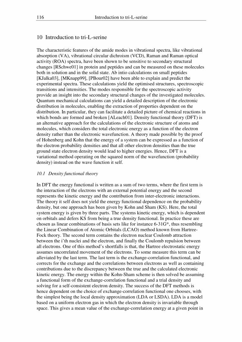
116 Introduction to tri-L-serine
10 Introduction to tri-L-serine
The characteristic features of the amide modes in vibrational spectra, like vibrational
absorption (VA), vibrational circular dichroism (VCD), Raman and Raman optical
activity (ROA) spectra, have been shown to be sensitive to secondary structural
changes [RSchwe01] in protein and peptides and can be measured on these molecules
both in solution and in the solid state. Ab intio calculations on small peptides
[KJalka03], [MKnapp99], [PBour02] have been able to explain and predict the
experimental spectra. These calculations yield the optimised structures, spectroscopic
transitions and intensities. The modes responsible for the spectroscopic activity
provide an insight into the secondary structural changes of the investigated molecules.
Quantum mechanical calculations can yield a detailed description of the electronic
distribution in molecules, enabling the extraction of properties dependent on the
distribution. In particular, they can facilitate a detailed picture of chemical reactions in
which bonds are formed and broken [ALeach01]. Density functional theory (DFT) is
an alternative approach for the calculations of the electronic structure of atoms and
molecules, which considers the total electronic energy as a function of the electron
density rather than the electronic wavefunction. A theory made possible by the proof
of Hohenberg and Kohn that the energy of a system can be expressed as a function of
the electron probability densities and that all other electron densities than the true
ground state electron density would lead to higher energies. Hence, DFT is a
variational method operating on the squared norm of the wavefunction (probability
density) instead on the wave function it self.
10.1 Density functional theory
In DFT the energy functional is written as a sum of two terms, where the first term is
the interaction of the electrons with an external potential energy and the second
represents the kinetic energy and the contribution from inter-electronic interactions.
The theory it self does not yield the energy functional dependence on the probability
density, but one approach has been given by Kohn and Sham (KS). Here, the total
system energy is given by three parts. The systems kinetic energy, which is dependent
on orbitals and defers KS from being a true density functional. In practice these are
chosen as linear combinations of basis sets like for instance 6-31G*, thus resembling
the Linear Combination of Atomic Orbitals (LCAO) method known from Hartree-
Fock theory. The second term contains the electron nuclear Coulomb attraction
between the i’th nuclei and the electron, and finally the Coulomb repulsion between
all electrons. One of this method’s shortfalls is that, the Hartree electrostatic energy
assumes uncorrelated movement of the electrons. To some measure this term can be
alleviated by the last term. The last term is the exchange-correlation functional, and
corrects for the exchange and the correlations between electrons as well as containing
contributions due to the discrepancy between the true and the calculated electronic
kinetic energy. The energy within the Kohn-Sham scheme is then solved be assuming
a functional form of the exchange-correlation functional and a trial density and
solving for a self-consistent electron density. The success of the DFT methods is
hence dependent on the choice of exchange-correlation functional one chooses, with
the simplest being the local density approximation (LDA or LSDA). LDA is a model
based on a uniform electron gas in which the electron density is invariable through
space. This gives a mean value of the exchange-correlation energy at a given point in

Introduction to tri-L-serine 117
space. If the expansion of the density, as which LDA can be regarded, is
supplemented with gradients of the density, a more complete description for
molecules is achieved. A widely used gradient corrected exchange functional is the
one proposed by Becke, which leaves the choice of correlation functional open. Here,
corrections like the Lee-Yang-Parr correlation functional (LYP) can be used. The
main method used in these calculations is the B3LYP, which is semi-empirically
determined hybrid method. The B3 exchange includes three different expressions for
the exchange with appropriate weight, determined by fitting to experimental data, thus
enabling a better fit to experiment and being applicable for the systems for which the
experimental data were (are) available. “The B3LYP hybrid method has also been
shown to give good results for systems which were not included in the
parameterization.”
10.2 Calculation of the vibrational spectra
At the basis of the theoretical treatment of spectroscopic features lies the ability to
predict transitions between different states. After the identification of ground state it is
possible to generate exited states by exposing the ground state to different radiations
fields. These excited states can have different origins, for example vibrational,
electronic, rotational or nuclear or electronic spin. By measurement of absorption of
incident light of a given frequency, polarisation and intensity it is possible to infer
something about the structural features of the investigated system [ASen84],
[MDiem84], [PBour02]. The main purpose of vibrational analysis is to assign spectral
features to structural features or units in the molecule. By comparing theoretical and
experimental spectra it should in theory be possible to determine the best candidate
for a structure in cases where only one conformer and species is present. However,
several conformers and species might be present, obscuring the interpretation.
Additionally pH effects, solvent polarity, solute concentration, and ionic strength
might need to be investigated as they all can influence and changes the molecule and
hence its spectra.
The assignment of frequencies to specific vibrational modes is important, in that it
connects the fluctuation in the 3-dimensional structure of the molecule. Molecular
properties, such as magnetic or electric dipole moments, can be defined as the
response of a wavefunction to an external perturbation. The description of the
perturbation of the energy can be made within the wavefunction picture, since it is
energy that is perturbed regardless of the perturbation which is applied. The
perturbation can for instance be due to an external electric field, an external magnetic
field or a change in the nuclear geometry.
The minimum energy structure is due to the fluctuations not fixed in space, and it is
therefore convenient to describe the molecular system by mass weighted coordinates.
This allows the potential energy to be Taylor expanded around the optimised structure
and giving a solution of the nuclear displacement in terms of internal coordinates. The
normal modes for the 3N-6 vibrational modes (for a non-linear molecule) can be
described in terms of linear combinations of these internal coordinates. A normal
mode calculation yields a description for the observed vibrations and the nuclear
displacements that is dependent on the optimised structure, the force field and atomic
masses. Mass-weighted coordinates can be transformed to normal coordinates, but
this still is not a convenient way to describe displacement like e.g. bond stretching.
Therefore normal coordinates are transformed to an internal coordinate system. The
118 Introduction to tri-L-serine
association of chosen internal coordinates and a frequency is made via the force
constants contribution to that frequency. This is called the potential energy
distribution (PED), which is a convenient way of assigning frequencies to vibrational
modes. Additionally one can use molecular visualization programs like Gauss View
and Molden to graphically display the molecular vibrations, but the PEDs are
quantitative descriptions, which depend on the choice of internal vibrational
coordinates. These are different from simple valence internal coordinates normally
used for Z-matrices in geometry optimizations or in molecular mechanic force fields.
In this study one conformer of the nonionic neutral and zwitterionic species of L-
serinyl L-serinyl L-serine (SSS or tri-L-serine), together with its cationic and anionic
species and the capped N-acetyl tri-L-serine N'- methylamide (NALSLSLSNMA)
analog were optimized with density functional theory with the Becke 3LYP hybrid
exchange correlation (XC) functional and the PW91 GGA XC functional and the 6-
31G* and aug-cc-pVDZ basis sets. Subsequently the vibrational absorption (VA),
vibrational circular dichroism (VCD), Raman and Raman optical activity (ROA)
spectra were simulated in order to compare them to experimentally measured spectra.
A comparison of the various ways to treat the effects of the environment and solvation
on both the structure and the spectral properties has been thoroughly investigated for
one conformer, with the goal to determine which level of theory is appropriate to use
in the systematic search of the conformational space for this and other small peptides
in aqueous solution, at low, medium and high pH levels. In addition, the effects of the
counterion, here Cl- anion, are also investigated.
10.3 Bibliography
[RSchwe01] R. Schweitzer-Stenner, (2001) J. Raman Spectrosc., 32, 711-732.
[KJalka03] K. J. Jalkanen et al., (2003) Vibrational Analysis of Various
Isotopomers of L-Alanyl-L-Alanine in Aqueous Solution: Vibrational
Absorption, Vibrational Circular Dichroism, Raman, and Raman
Optical Activity Spectra, International Journal of Quantum Chemistry,
92, 239-259.
[MKnapp99] M. Knapp-Mohammady et al., (1999) Chem. Phys., 240, 63-77.
[PBour02] P. Bour et al., (2002) Ab initio quantum mechanical models of peptide
helices and their vibrational spectra, Biopolymers, 65, 1, 45-59.
[ALeach01] A. R. Leach, Molecular Modelling, Principles and Applications,
Pearson Education Limited, 2nd
edition, 2001.
[ASen84] A. C. Sen & T. A. Keiderling, (1984) Vibrational Circular Dichroism
of Polypeptides. III. Film Studies of Several α-Helical and β-sheet
Polypeptides, Biopolymers, 23, 1533-1545.
[MDiem84] M. Diem et al., (1984) Determination of Peptide Conformation via
Vibrational Coupling: Application to Diastereoisomeric Alanyl
Dipeptides, Biopolymers, 23, 1917-1930.

INSTITUTE OF PHYSICS PUBLISHING PHYSICAL BIOLOGY
Phys. Biol. 3 (2006) S63–S79 doi:10.1088/1478-3975/3/1/S07
The VA, VCD, Raman and ROA spectraof tri-L-serine in aqueous solutionV Wurtz Jurgensen1 and K Jalkanen1,2,3
1 Quantum Protein (QuP) Centre, Department of Physics, Technical University of Denmark, Bldg 309,DK-2800 Kgs Lyngby, Denmark2 Laboratory of Physics, Helsinki University of Technology, PO Box 1100, 02015 TKK, Otakaari 1,Espoo, Finland3 Nanochemistry Research Institute, Department of Applied Chemistry, Curtin University of Technology,GPO Box U1987, Perth, Western Australia 6845, Australia
Received 9 December 2005Accepted for publication 16 January 2006Published 22 February 2006Online at stacks.iop.org/PhysBio/3/S63
AbstractThe structures of one conformer of the nonionic neutral and zwitterionic species of L-serinylL-serinyl L-serine (SSS or tri-L-serine), together with its cationic and anionic species and thecapped N-acetyl tri-L-serine N′-methylamide analog were optimized with density functionaltheory with the Becke 3LYP hybrid exchange correlation (XC) functional and the PW91 GGAXC functional and the 6-31G∗ and aug-cc-pVDZ basis sets. Subsequently, the vibrationalabsorption, vibrational circular dichroism, Raman and Raman optical activity spectra weresimulated in order to compare them to experimentally measured spectra. In addition, wecompare to previously reported studies for both structural determination and spectralsimulations and measurements. A comparison of the various ways to treat the effects of theenvironment and solvation on both the structure and the spectral properties is thoroughlyinvestigated for one conformer, with the goal to determine which level of theory is appropriateto use in the systematic search of the conformational space. In addition, the effects of thecounterion, here Cl− anion, are also investigated. Here we present the current state of the art innanobiology, where the latest methods in experimental and theoretical vibrationalspectroscopy are used to gain useful information about the coupling of the nuclear, electronicand magnetic degrees of freedom and structure of tri-L-serine and its capped peptide analogwith the environment.
S This article has associated online supplementary data files
Introduction
One approach for the determination of protein and peptidesecondary structure from the spectroscopic data is tooptimize the geometry for all possible low energy structuresof the system with density functional theory (DFT) usingthe appropriate exchange correlation (XC) functional andappropriate treatment of the environment, and for theseoptimized structures simulate the spectra measured. This isespecially important for new novel flexible peptides, whichcan assume various structural and functional states dependingon small changes in the environment. For the conformerswith the lowest energies and predicted to be present under theconditions of the experiment, the vibrational absorption (VA),
vibrational circular dichroism (VCD), Raman and Ramanoptical activity (ROA) spectra can be simulated and comparedto the experimental data. The best match is, in theory, thecandidate for the structure in cases where only one conformerand species is present. In some cases, more than oneconformer or species may be present at the given temperaturein the solution for which the intensity measurements weremade. This will complicate the interpretation of the measuredspectra and, therefore, temperature-dependent studies maybe required. In addition, the effect of pH, solvent polarity,solute concentration and ionic strength may all also have to beinvestigated. In many cases due to the pKas of the N-terminal,C-terminal and side chain groups, the solution’s pH needs tobe carefully controlled by buffering conditions.
1478-3975/06/010063+17$30.00 © 2006 IOP Publishing Ltd Printed in the UK S63

V W Jurgensen and K Jalkanen
The aim for the present study is to optimize the structuresof the various species of tri-L-serine (neutral nonionicand zwitterionic, anionic and cationic) for a representativeconformer and to simulate the VA or infrared (IR) intensities,VCD intensities, Raman intensities and ROA intensities andnuclear magnetic resonance (NMR) shielding tensors for thesefour species. Additionally, one conformer of tri-L-serine’scapped analog (NALSLSLSNMA) has also been determined.The start configuration (conformer) was chosen to be thelinear structure since a crystal structure for the peptide isnot available. A search for the lowest energy conformer andother low energy conformers will be performed for all speciesonce the adequate level of theory to do so is determined.The level of theory to adequately treat the effects due tothe environment, solvation, hydrogen bonding and pH on thestructures, vibrational frequencies, and VA, VCD, Raman andROA intensities needs to be documented before one undertakesthe very expensive systematic potential energy surface search.It is not feasible to perform systematic searches at all levels oftheory at this time, nor is scientifically expedient.
The two neutral species of tri-L-serine that wereinvestigated are the nonionic NH2–· · ·–COOH and thezwitterionic NH3
+–· · ·–COO− forms. This allows one tocompare the spectroscopic features of the various specieswith each other and also with the experimental spectra ofthe tri-peptide in solution. One generates spectra that canbe compared to those measured on tri-L-serine in solutions ofnonpolar and polar solvents and those measured on tri-L-serinein the gas phase, in the powdered state or dissolved in a KBrpellet. With the recent increased use of mass spectroscopyand molecular beam experiments, the vibrational spectra ofmany peptides and their fragmentation products have beenmeasured under a variety of experimental conditions. It isnecessary to simulate spectra for the conditions relevant forthese experiments, and not strictly for the measurements onaqueous solutions. Simulated spectra can be used to determinewhether the peptide’s most dominant species is the zwitterion,anion or cation in the solution measured, and whether thechosen geometry (structure or conformer) is the dominantconformer present for the given species. In many cases,the measurements are made for solutions where the exactpH is not known. Here, by analyzing the spectra, one mayactually be able to determine the pH by determining the speciespresent. This will extend the use of VA, VCD, Raman and ROAmeasurements to determine pH and ionic strength of aqueoussolutions of amino acids and peptides. This is extremelyimportant when many species are all present, and not a singleconformer and single species.
The possibility of more than one species and conformerbeing present for the experimental conditions of themeasurement further complicates the spectral interpretation.Therefore, calculations on the anionic and cationic species oftri-L-serine were made in order to be able to distinguish thespecies present under conditions present in the experiments.In addition to the continuum model calculations, we haveadditionally solvated the cation/Cl− counterion complex withexplicit water molecules. Here one seeks to determinehow well the Onsager and PCM continuum models are able
to represent/reproduce the effects due to explicit hydrogenbonds. Finally, we have embedded this complex withinboth a spherical cavity (Onsager model) and a molecularcomplex cavity (PCM model), to see how well the combinedhybrid model does, that is, how well the explicit water modelsimulates the effects due to the strongly interacting hydrogenbonded water molecules and how well the continuum models(Onsager or PCM) simulate the effects due to the bulk watermolecules and the water molecules near the hydrophobicgroups, but not strongly interacting with the peptide. Finally,the results at all levels of theory are compared to otherreported theoretical results for tri-L-serine and the availableexperimental data, which is the ultimate benchmark for allsimulations which seek to model real biological systemsin their native environments. The last species for whichcalculations were performed is the capped analog: N-acetyltri-L-serine N′-methylamide. To determine the spectra ofthe tri-L-serine sequence as it occurs in a large protein onesimulates the spectra of the tripeptide’s capped analog.
Materials and methods
Density functional theory
The calculations were performed with Gaussian 98 and 03at the DFT level of theory with the Becke 3LYP hybrid XCfunctional (DFT-B3LYP) and the Perdew Wang generalizedgradient approximation (GGA) XC functional (DFT-PW91)with the 6-31G∗ and aug-cc-pVDZ basis sets. At these levelsof theory we have additionally calculated the Hessian, theatomic polar tensors (ATP) and the atomic axial tensor (AAT),which allows us to calculate the dipole- and rotational strengthsrequired to simulate the VA and VCD spectra. Furthermore,the electric dipole electric dipole polarizability derivatives(EDEDPD) were calculated in order to simulate the Ramanscattering spectra. In addition, geometry optimizations wereperformed at the DFT-B3LYP and DFT-PW91 levels with theOnsager continuum model for the neutral zwitterionic speciesand its anionic and cationic forms. The Onsager continuumis a reaction field model, which allows one to simulatethe solvation effects on the properties of the solute withoutconsidering explicit solvent molecules [1]. It representsthe effects due to the bulk solvent, but does not includethe direct interactions between the solute and the solvent.A thorough description of both DFT and its extension tosimulate vibrational spectra can be found in [2–10]. At theoptimized Onsager geometry, atomic axial tensors (AAT) werecalculated without the Onsager model. The DFT-B3LYPlevel of theory has been shown to be able to reproduce theVA and VCD spectra for the alanine dipeptide quite well.This level of theory with the 6-31G∗ basis set was chosenas a compromise between high accuracy and computationalcost for treating the effects due to explicit water moleculesand the combined hybrid approach [8, 9]. Additionally, theVCD spectra have been simulated using the PCM model, amore sophisticated continuum solvent model, to represent theeffects due to the solvent. Our previous work involved usingthe Onsager continuum model [8, 9]. Here one wishes to
S64
The VA, VCD, Raman and ROA spectra of tri-L-serine in aqueous solution
test the more elaborate PCM model for treating the effectsdue to the aqueous environment. In addition, the structure ofNALSLSLSNMA with the 6-31G∗ basis set at the DFT-B3LYPlevel has been determined. Previously, we have recommendedthe large aug-cc-pVDZ basis set for high quality Raman andROA spectral simulations for phenyloxirane [11], but in thiswork the smaller basis set (6-31G∗) that we have previouslyused for our modeling studies on LA and NALANMA,which gave us qualitative agreement with the experimentallymeasured ROA spectra for these two molecules in an aqueousenvironment, has been used [8, 9]. Additionally, the VA,VCD, Raman and ROA spectra of NALSLSLSNMA with the3-21G split valence basis set and at the DFT-B3LYP levelhave been simulated. Here one documents how well this splitvalence basis set does. Previously a minimal basis set forthe semi-empirical based DFT method, the so-called SCC-DFTB method, has been used to determine the optimizedstructures and Hessians for NALANMA, oxirane, thiiraneand Leu-enkephalin [12]. Unfortunately the tensors requiredto simulate the VCD, Raman and ROA spectra are not yetimplemented, and it is not even yet known whether the tensorscalculated with a minimum basis set would be even worthpursuing, but from previous studies, the prospects appear tobe very low. A more practical and feasible alternative is touse a split valence basis set like the 3-21G basis set, but thislevel of theory may also be inadequate. The inclusion ofpolarization functions is most likely to be important for evenqualitatively representing the linear response properties due tothe time varying electric and magnetic fields. Here the VA,VCD, Raman and ROA spectra for NALSLSLSNMA havebeen simulated with the 3-21G level of theory to documentwhether this level of theory is actually worth pursuing inthe context of extending the SCC-DFTB method for thesimulation of the VA, VCD, Raman and ROA intensities. Itis very important to extend the current SCC-DFTB theory totreat the electronic and magnetic response properties of themolecule in biological systems in their native environment.The tensors and their derivatives with respect to nucleardisplacements and velocities are not only important forsimulating the intensities of the vibrational transitions, butalso for deriving the forces which bind the molecules to eachother (complex and aggregation phenomena) and to ligands(drug molecules, be they inhibitors or substrate analogs).Hence theoretical vibrational spectroscopy can not only addto the understanding for experimental spectroscopists, but alsofor molecular biologists, physical biologists and biochemists,who seek new theoretical and experimental methods tounderstand the structure, function and mechanism of actionof their nanomachines (proteins, self-assembling aggregatesof proteins, protein/nucleic acid complexes and glycosolatedproteins).
By using DFT-PW91 GGA XC functionals the nonlocalexact exchange from the DFT-B3LYP XC functional is notused. This saves on computational expense and programingand has been recommended by many solid state physicsgroups for this reason. Additionally, the optimized effectivepotential (OEP) method has been suggested as an alternativeto exact nonlocal exchange [13]. The OEP method allows
one to develop a local exchange functional that satisfies manycriteria which are not satisfied by nonOEP local exchangefunctionals, one criterion being that an electron does notinteract with itself (self interaction). The exact exchange termis nonlocal and expensive to calculate hence the search forexchange terms which are local. The exact exchange andCoulomb terms exactly cancel for a one-electron system, butfor many local exchange functionals used, a self-interaction(SI) term exists, which is clearly in error. Recently thegroup of Bartlett has extended the OEP method, which wasoriginally developed to generate local exchange functionalsfor atoms, to generate local OEP correlation functionals basedon MP2 correlation energies and potentials and subsequentlybased on coupled cluster correlation energies and potentials.They have called this methodology ab initio DFT since itallows for a systematic improvement of the XC functionals, incontrast to the previously developed XC functionals. The OEPexchange and correlation functionals are systematically betterwith respect to their convergence properties, a problem notedby the Bartlett group which previously prevented the generaluse of the OEP method [14]. This methodology presents away to systematically improve upon the XC functionals usedwithin the DFT method. An approximation to the rigorousOEP method developed by Krieger, Li and Iafrate is alsovery accurate and computationally feasible [15]. This hasreally greatly improved the previous limitations of DFT. Theproblems with calculating charge transfer excitations havebeen addressed by the Handy group [16]. The problems withcalculating excited state energies by the static limit and byincluding dynamical effects have been addressed by the groupsof Gross, Aldrichs and Berands among others [17]. Finally, theproblem of the treatment of dynamic and static correlation andvan der Waals forces (interactions) and hydrogen bonding,very important for modeling biological systems, have alsorecently been addressed [18, 19]. Hence the latest DFTimplementations are fast approaching the highly correlatedwavefunction methods in accuracy and applicability, but withless cost than the full wavefunction based methods, but ofcourse with more cost than the originally formulated DFTmethods. The synergistic relation between wavefunction anddensity functional based quantum mechanics has never beenmore fruitful than it now is and it appears to be evolving withan ever increasing rate. Additionally, Green’s function integralapproaches, like the GW method, are also contributing to thepicture, especially with respect to the treatment of excitedelectronic states [20]. Here the time-dependent extension ofDFT still has its problems. What remains to be done is forthese new ab initio DFT XC functionals to be implemented inopen source DFT codes such as SIESTA [21] and ABINIT [22]and also for the linear response properties to be implementedwhich will allow for the calculation of all of the propertiesrequired to simulate the VA, VCD, Raman and ROA spectra.This will allow for the promulgation of these methods to thefull research communities.
To treat the effects due to the environment (solvent) thepolarized continuum model (PCM) incorporates electrostatic,dispersion–repulsion contributions to the molecular freeenergy and cavitation energy [23]. However, at the optimized
S65

V W Jurgensen and K Jalkanen
geometries obtained with the PCM model with the Gaussianprogram for the charged species, some of the Hessiansgave us negative eigenvalues. It was originally postulatedthat this problem originated due to the lack of an origin-independent definition of the electric dipole moment forcharged systems. Subsequently calculations were performedwith the Cl− counterion in close proximity to the positivelycharged ammonium group to give us a well-defined neutralspecies for the tri-L-serine cation–Cl− anion complex. Thedevelopers of the PCM model have also noted that this modelmay have problems for charged systems [23]. Here we madethe system neutral by adding the Cl− anion to the tri-L-serinecation. Initially we did not solvate the system, but performedgeometry optimizations for the salt bridge (ion pair state)complex. This did not solve the problem, and the cation/anioncomplex was subsequently explicitly solvated with ‘22’ watermolecules. In addition to the explicit water treatment, wehave additionally embedded the tri-L-serine cation/Cl− anioncomplex (solvated system) within a spherical cavity (Onsagercontinuum model) and a cavity that encloses (has the shapeof ) the hydrated complex (PCM continuum model). Due toconvergence problems with the geometry optimizations withthe PCM for the complex, we do not present the complex/PCMresults here. Note that the effects due to the solvent have beenhypothesized to be small, but in the case of the hydrogenbonding this approximation is not the case.
The goal here has been to determine the level of theoryand solvent treatment to use for the future systematic potentialenergy search (scan) for this molecule and its various species,but along the way we have encountered some fundamentalproblems with the treatment of the solvent environment. Whathas further complicated this work is that, in addition tohaving multiple conformers present under the conditions ofthe experiment, there may also be multiple species, and if theconcentration is too high, aggregate formation. In additionto the problem of conformational sampling and averaging,one is faced with the additional problem of species samplingand averaging and finally the sampling and averaging ofthe solvent degrees of freedom. With the proton possiblymoving back and forth between two atoms to interconvertbetween species, the conformational equilibrium is not justthermodynamically determined, as assumed by many, but alsokinetically determined. Hence the ideas of thermodynamicaveraging may need to be re-explored and the idea of kineticaveraging may need to be explored. The whole idea of a meanfield approach may also need to be re-thought. Hence one mustbe very careful when analyzing the distribution of all of thespecies and conformers of the species when one is analyzingthe spectra of a biological sample. In addition, the time scaleof the measurement and the physics of the process need to beconsidered, whether one determines an average structure orone determines a superposition of structures. Here in additionto the solvent molecules which are strongly hydrogen bondedwith the polar portions of the peptides, we also have to properlysample and average the solvent molecules which form thecages around the nonpolar groups (the so-called hydrophobiceffect) and the counterions; the solvent molecules which arein contact with these solvent molecules, and whose motions
are strongly coupled with the aforementioned, also need to beconsidered. Hence, there is lack of real progress in this area,even though the basic ideas and formulation of the problemare relatively straightforward! In this work, we also have notcompletely solved all of these problems, but have addressed thequestion of how to couple the explicit and continuum solventmodels to be able to simulate the VA, VCD, Raman and ROAspectra of biomolecules in the aqueous media. This is anextension of our previous work on NALANMA where weshowed to simulate the VA, VCD, Raman and ROA spectra ofthis molecule we needed to include explicit water molecules[9, 10]. In addition, the structure found, the PII structure, isnot even a minimum on the gas phase potential energy surface.Hence the NALANMA plus four water molecule complex isthe real species of interest. That this is the case has beenverified by recent NMR experiments, which previously couldnot be interpreted. This new paradigm has not only allowed forthe interpretation of the VA, VCD, Raman and ROA spectraof NALANMA [9], but also of the NMR spectra [24]. In thenext section, we give a brief overview of the theory requiredto calculate the tensors required to simulate the VA, VCD,Raman and ROA spectra of tri-L-serine. For the equations thereader can see our previous works on NALANMA [8–10].
Theoretical treatment of spectroscopic features
At the basis of the theoretical treatment of spectroscopicfeatures lies the ability to predict transitions between differentstates. After the identification of the ground state, it ispossible to generate exited states by exposing the ground stateto different radiations fields. These excited states can havedifferent origins, for example vibrational, electronic, rotationalor nuclear or electronic spin. By measurement of absorption ofincident light of a given frequency, polarization and intensity,it is possible to infer something about the structural featuresof the investigated system [25–27]. The main purpose ofvibrational analysis is to assign spectral features to structuralfeatures or units in the molecule. Molecular properties such asthe electric dipole moment can be defined as the response of thewavefunction (or electron density) to an external perturbation[7, 11].
The description of the perturbation of the energy can bemade within the wavefunction picture, since it is energy thatchanges regardless of the perturbation that is applied. Theperturbation can for instance be due to an external electricfield, an external magnetic field or a change in the nucleargeometry. Extensive treatment of the theory behind spectralsimulations, i.e. obtaining the tensors required to simulatethe VA, VCD, Raman and ROA spectra, can be found invarious books and journals [7–11]. The theory for VA andVCD spectral simulations is thoroughly discussed in [28–43],whereas the theory behind Raman scattering and ROA spectralsimulations previously have been covered in [8–10].
Experimental infrared or vibrational absorption, vibrationalcircular dichroism and Raman spectral measurements atBruker AG, Ettlingen, Germany
L-serinyl-L-serinyl-L-Serine (SSS or tri-L-serine) waspurchased as a lyophilized powder from Bachem
S66

The VA, VCD, Raman and ROA spectra of tri-L-serine in aqueous solution
Feinchemikalien AG (>98% purity TLC) and was notdissolvable in pure deionized H2O. The theoretical pI forSSS was calculated to be 5.24 [44]. The FTIR spectrawere recorded at room temperature with a Bruker IFS 66/Sinstrument. A liquid cell with a CaF2 window and 6 mmpath length was used for the solution VA spectroscopy. TheVCD spectra were measured at room temperature with aBruker IFS 66/S, PMA 37 instrument and obtained at 4 cm−1
and 6 cm−1 resolutions and a photo-elastic modulator (PEM)set to 1/4 wave at 1500 cm−1. VCD and VA spectrawere measured against pure solvent and against pure KBr,respectively. The tri-peptide was dissolved in approximately0.1% HCl solution with 50 mg ml−1, i.e., 179 mMfor the VA measurements. Tri-L-serine was also mixed withKBr, 1 mg substance in 201 mg KBr and compressed into asolid pellet, which was used for both the VA and VCD spectralmeasurements.
The frequency range for VA spectra of tri-L-serine in HClobtained in the CaF2- cell had a range from 1000 to 1800 cm−1
and spectral resolution 4 cm−1. Due to low optical density ofSSS in HCl, it was not possible to obtain a VCD spectrum ofthis solution. The frequency range for the VA spectrum fortri-L-serine in KBr pellet was 500–4000 cm−1 with a spectralresolution of 4 cm−1. For the VCD spectrum of the pelletthe range was 1000–1800 cm−1, with a spectral resolution of6 cm−1. Finally a saturated solution of tri-L-serine in CCl4was prepared for both VA and VCD measurements, thoughthe optical density for VCD was not high enough.
Experimental infrared or vibrational absorption, vibrationalcircular dichroism and Raman scattering spectralmeasurements at Thermo Electron Corporation, Madision,WI, USA
Raman scattering: spectra were obtained at Thermo ElectronCorporation, Madison, WI, USA. For the experiments atThermo Electron Corporation 25.32 mg tri-L-ser powder wasdissolved in 500 ml of 0.25 M HCl, yielding a pH of 0.93and a concentration of 180 mM. Only Raman scatteringmeasurements were able to be measured on the solutions. Theconcentration was too high to allow for good VA and VCDmeasurements. The Raman measurements were made at twodifferent wavelengths, as shown on the experiment spectra.
DFT with the Becke 3LYP hybrid XC functional
All the peptides were built using either the program GaussView[45] or Molden [46] with all backbone atoms lying in thesame plane, i.e., the all-trans configuration with side groupsalternately pointing up and down. Bond angles were initiallychecked so that they corresponded to ideal sp2 and sp3
hybridizations. The bond lengths were set to standard valuesobtained from a built in library in GaussView. These structuresCartesian coordinates were used as input for Gaussian 98 and03. Geometry optimization rendered an optimized structureand corresponding electronic energy. The VCD intensitiesare calculated with Gaussian 98 and 03, in addition to thenormal mode frequencies and VA or IR intensities. To getthe VA spectra the APT were calculated, as well as the AAT
additionally necessary for the VCD spectra. Raman intensitieswere computed with Gaussian 98 and 03 as well, and forthe simulation of the Raman spectra, the EDEDPD neededto be calculated. Raman intensity calculations are defaultfor SCF frequency calculation, but can be specified for DFTand MP2 calculations to produce the intensities by numericalcalculations via finite field perturbation theory.
Results and discussion
The optimized structures represent only a local energyminimum for each species. The most important dihedralangles, which determine the conformer for tri-L-serine, ofall the species investigated are given in supplementary (sup)table S1(b) together with all calculated bond lengths in suptable S1(a) (available from stacks.iop.org/PhysBio/3/S63).The atom numbering in the tables for the structural parametersis shown in sup figures S1(a)–S1(h) and in figures 1(a) and (b).There are not large differences in the bond lengths calculatedfor the different tri-L-serine species. The species for whichthe values diverge the most from the mean values is thezwitterionic species calculated without the Onsager continuummodel. For instance, the length of the CO bond differs fromthe mean value by 0.012 A, while the bond lengths for theother CO bonds differ by not more than 0.002 A from themean value. This can be understood in light of the fact that allother ionic species were calculated within the two continuummodels (Onsager and PCM).
Assignment and description of the vibrational modes
The interaction of electromagnetic radiation with molecularvibrations is generally described in terms of normal modesof the system investigated. The normal modes belongingto the peptide group are the so-called amide modes: amideI, II and III (AI, AII and AIII). AI is usually described asa pure CO stretching mode, where (CO s) is the dominantcontribution to the eigenvector, but can also contain, forinstance, some mixture of CCN deformation (CCN d). AIis normally accredited to the region around 1600–1700 cm−1
[47–49]. AII is generally considered less structure sensitivethan AI and AIII, and is generally attributed as the out-of-phase combination of CN s and NH in-plane bend (ib). AIIis normally found around 1550 cm−1. AIII is reported morestructure sensitive than AI, and in general described as an in-phase combination of CN stretch and NH ib. AIII is commonlyfound around 1250 cm−1. To assign the modes one mustdefine a set of internal coordinates which can be used in theso-called vibrational analysis. One can then use these internalcoordinates to assign modes based on the potential energydistributions (PEDs). In sup table S2 we define the internalcoordinates and in sup tables S2(a), S2(b) and S2(c) we givethe vibrational frequencies (ν i), the PEDs based on the internalcoordinates given in sup table S2, the dipole strengths (Di), therotational strengths (Ri) and the Raman scattering intensities(Ram) for the zwitterionic species. The atom numbering isas given in sup figure S1(b). In sup table S3 we definethe internal coordinates and in sup table S3(a) we give the
S67

V W Jurgensen and K Jalkanen
(a) (b)
Figure 1. (a) Tri-L-serine cation II, (b) tri-L-serine cation II + Cl− anion solvated with 22 water molecules + Onsager continuum model(best model).
vibrational frequencies ν i, the PEDs based on the internalcoordinates given in sup table S3, the Di, the Ri, and the Ramfor the nonionic neutral species, atom numbering given in supfigure S1(a).
In sup table S4 we define the internal coordinates andin sup table S4(a) we give the ν i, the PEDs based on theinternal coordinates given in sup table S4, the Di, the Ri andthe Ram for the capped species, atom numbering given in supfigure S1(g). In sup table S5 we define the internal coordinatesand in sup tables S5(a) and S5(b) we give the ν i, the PEDsbased on the internal coordinates given in sup table S5, the Di,the Ri and the Ram for the anionic species, atom numberinggiven in sup figure S1(d ). In sup table S6 we define theinternal coordinates and in sup tables S6(a)–S6(e) we give theν i, the PEDs based on the internal coordinates given in suptable S6, the Di, the Ri and the Ram for the cationic species,atom numbering given in sup figure S1( f ). In sup table S7 wedefine the internal coordinates and in sup tables S7(a)–S7(c)we give the ν i, the PEDs based on the internal coordinates givenin sup table S7, the Di, the Ri and the Ram for the cationic/Cl-anioinic solvated species, atom numbering given in supfigure S1(h). Figures 1(a) and (b) show the structures of twodifferent ways to model the cationic species of tri-L-serine:(a) cation II + PCM continuum model and (b) cation
II + Cl− anion solvated water complex embedded withinan Onsager solvation sphere. In sup figures S1(a) neutral,S1(b) zwitterion, S1(c) zwitterion with Onsager, S1(d ) anionI, S1(e) anion II, S1( f ) cation I, S1(g) capped tri-L-serineand S1(h) cation II, solvated and Cl− anion are shown forthe other species found to date. Note that for the solvatedspecies, the positions of the water molecules may change(the hydrogen bonded water–peptide–Cl− anion network isvariable). Hence the internal coordinates of the cation and theindividual water molecules are stable, but the other internalvibrational coordinates may change. Hence which set ofinternal coordinates to use for these complexes is an open areaof research, which we are investigating. For each snapshot(local minimum), the set of internal coordinates is clearlydefined, but not necessarily the same with the previous step.Hence in sup table S7 not all internal coordinates are labeled,and hence the PEDs in sup tables 7(a), 7(b) and 7(c) are notall labeled, but ν i, Di, Ri and Ram are all given.
For the calculated species the amide modes are not allpure modes, but contain mixing to different degrees, seesup tables S8–S11. Amide I for anion I and II containsalso mixtures from stretching of the carboxyl group (R19,20),while cation II’s AI mode contains mixing with a CN stretchand a CNN deformation, consistent with the definition of the
S68

The VA, VCD, Raman and ROA spectra of tri-L-serine in aqueous solution
coordinate R76 in sup table S6 as assigned in sup table S8.The capped species has mixtures of different C=O stretchesand one mixed with a CN stretch. The neutral species hasjust pure C=O stretches, where R20 is a CO stretch of thecarboxyl group. For the zwitterionic species without theOnsager continuum model, the AI mode consists of a C=Ostretch together with a CN stretch, except for R20 and R21
which again is the stretching mode of the carboxyl group.The zwitterionic species within the Onsager solvation sphereis made up of pure C=O stretches except for the carboxylgroup. AII modes for all calculated types (species) are asgiven by their PEDs in sup table S9. For most species theamide modes are pure, expect for the cations, where there isconsiderable mixing with, for instance, R52, which is a H–C–H scissor. One exception is given by the amide modes forthe cationic species calculated at the higher level of theoryor larger basis sets, see sup tables S8, S9 and S10, as well assup table S6(c) (B3LYP/aug-cc-pVDZ, PCM), sup table S6(d)(PW91/aug-cc-pVDZ, PCM) and sup table S6(e) (B3LYP/6–31G∗, PCM). AIII modes for all conformers, given by PEDsand the definition of in-phase combination of CN stretchingand NH in-plane bend, are found in sup table S10. The C–Hdeformation of methine is sometimes also considered anAIII mode and can for all calculated species be found insup table S11. All amide III modes show extensive mixing,for both types of modes, except for the in-phase combinationof CN stretching and NH in-plane bend of the cationicspecies calculated with the larger basis set (aug-cc-pVDZ),sup table S10. Diem and coworkers have shown that theamide III mode is only pure amide III in the model compoundN-methyl acetamide [26]. In their pioneering work onisotopomers of L-alanyl-L-alanine, they showed that the twoCH methine deformation modes on the N- and C-terministrongly couple with the amide III modes, mixing to suchan extent that there are actually 5 modes, two methine for eachCα–H group and what had been called the amide III mode.Subsequently, we confirmed this assignment in our theoreticalinvestigation on the isotopomers of L-alanyl-L-alanine [50].
Comparison of the calculated zwitterionic species, supfigures S4–S6, shows substantial differences in peak positionsand intensities of the IR spectra, see sup tables S2(a)–S2(c)and sup table S8–S10. The IR intensities are found to belarger using the Onsager model. The experimental IR spectrumof water has intense modes at 3500 and 1700 cm−1 that theOnsager continuum model does not treat explicitly [1]. Thesolvent water is treated as a spherical dielectric cavity of radiusao with the dielectric constant ε = 78 representing the solventpolarity in which the molecule is embedded. Note that theinteraction term in the Onsager model is a function of theelectric dipole moment of the molecule, molecules with noelectric dipole moment will not experience a solvent effect.This could explain the intensity difference seen betweenthe two models, as the shapes of the cavities are differentand the interaction Hamiltonians are different. For moredetails see [23]. The zwitterionic species calculated with alarger basis set (aug-cc-pVDZ) and with the PCM model setsitself apart from the previously calculated spectra, see supfigure S6. The amide I modes are shifted substantially towards
lower frequencies and are located around 1600 cm−1, see suptable S8, and are considerably more intense.
As expected the intensity of AIII is smaller than AII,which is as intense as AI or more dominant. AII is theleast sensitive to structure of the three amide modes and thelargest differences are observed for AIII as would be expectedfor structural changes seen for the dipolar ion calculatedwith the two different methods. A more extended structure,sup figure S1(c), is observed for the zwitterion optimizedwithin the Onsager continuum model, compared to a muchmore bent conformation, sup figure S1(b), for the methodwhich does not treat the solvent. By analyzing the vibrationalmodes with the GaussView program, one can see that thevibrational modes of the zwitterion computed with the Onsagercontinuum model are more due to displacements all over themolecule (delocalized modes) than of the zwitterion computedin ‘pure’ gas phase where the modes are due to a single or afew dominating displacements (localized modes) [45].
The VCD spectra differ to the same extent as theIR spectra. The Onsager continuum model without theinclusion of explicit water molecules does not appear to beadequate to model the spectra tri-L-serine in aqueous solution.In addition, the spectra appear to be greatly modified bythe continuum model. One of the problems inherent in theOnsager continuum model is the shape of the cavity. Therecommended procedure to determine the cavity radius isto perform a volume calculation. We have followed therecommended procedure and then noted that the cavity doesnot appear to enclose the whole molecule or complex when wehave combined the Onsager continuum with our explicit watermodel. By using the Molden program, one is able to see thesize of the box which fully encloses the molecule or complex.Here we have seen that the problems that some groups havereported with this model may be due to part of the moleculeand (or) complex (explicit water molecules) lying outside thecavity. We recommend that the previously reported Onsagerresults should be checked to see that either the molecule and(or) molecular complex was fully enclosed with the sphericalcavity. If not, these calculations should be repeated withlarger cavity radii. But in this case there is probably a largepercentage of the cavity that is now not filled with solvent.Here one has two possibilities, to go to a more physical cavity,for example the PCM model, or to fill the spherical cavityso that the cavity is filled with water molecules. Anotherpossibility is to develop a model with a rectangular cavity, tomatch the periodic boundary conditions and shapes which havebeen utilized in the solid state physics and condensed matterphysics community. Here the two groups of researchers canreally learn from each other. Indeed we have initiated a projectwhere we are now modeling and implementing new cavitymodels to treat the problem of solvation and solvent effects.In this report, we only present our results utilizing the Onsagerand PCM continuum models alone and in combination withoutexplicit water model.
Comparing the spectra of all calculated species,sup figures S4–S11, one sees quite different spectra,where both peak frequencies and intensities are distinct.The most remarked changes occur for higher frequencies
S69

V W Jurgensen and K Jalkanen
500 1000 1500 2000 2500 3000 35000
0.1
0.2
0.3
Ram
an
tri-L-serineexperimental spectra
500 1000 1500 2000 2500 3000 3500-0.0002
-0.0001
0
0.0001
0.0002
∆ A
bsor
banc
e
500 1000 1500 2000 2500 3000 3500
Wavenumber [cm-1
]
00.05
0.10.150.2
0.25
Abs
orba
nce IR-absorption of tri-L-ser in KBr-pellet
VCD of tri-L-ser in KBr-pellet
Raman of tri-L-ser in powder
Figure 2. Experimental VA, VCD and Raman spectra for tri-L-serine in KBr pellet and powder.
1000 1250 1500 1750 2000 2250 2500 2750 3000
Wavenumber [cm-1
]
-0.02
-0.01
0
0.01
0.02
0.03
Abs
orba
nce
VA-spectrum of tri-L-ser 179 mM in app. 0.1 % HCl
IR-absorption of tri-L-ser in HCl
Figure 3. IR absorption spectra of tri-L-ser in approximately 0.1% HCl.
(above 2000 cm−1), where all ionic-species peak intensities arelower than those from the capped-, neutral- and zwitterionic-species (without Onsager). That is, peak intensities forhigher frequencies are dampened within the Onsager solvationsphere, something that does not apply at all for the zwitterionicspecies calculated within the PCM model. All AI modes arerelatively similar by exhibiting intensities around 500–600,and are found in the same frequency range between 1800 and1700 cm−1, sup table S8. Both anions constitute exceptions,by having AI modes with intensities around twice that value,sup figures S7 and S8, sup tables 5(a) and (b), as well as allspecies calculated by PCM. The frequency of AI of the cationcalculated with PW91 is, however, considerably lower at
1627 cm−1. The amide II is the most prominent peak below2000 cm−1 in all calculated spectra, except for the cappedand the neutral species where the amide I region has the sameintensity. But also for the cation II and anion II, amide I ismore intense than AII, sup tables S6(b) and S5(b), as wellas the spectra calculated with the PCM model, here AII andAI are equally intense or AI is the dominating mode, suptables S6(c)–S6(e).
VA spectrum of tri-L-serine in KBr and in HCl solution
The peaks of VA spectra for the tri-L-serine/KBr pellet and thecompound in solution coincide, see figures 2 and 3. There are,
S70

The VA, VCD, Raman and ROA spectra of tri-L-serine in aqueous solution
Ram
an in
tens
ity
tri-L-serine cation IIcalculated at B3LYP/aug-cc-pVDZ with PCM
-800
-400
0
400
800
∆ε x
10-4
0 500 1000 1500 2000 2500 3000 3500 4000
Frequency [cm-1
]
0
600
1200
1800
ε
0 to 2000 cm-1
x 30
Figure 4. Calculated VA, VCD and Raman spectra for cation II with B3LYP/aug-cc-pVDZ and PCM.
however, some differences: solution peaks are much broaderand slightly shifted towards higher wave numbers, except for1556 cm−1 in KBr pellet, which is shifted down to 1546 cm−1
in solution (blow-up of the amide I region can be found insup figure S2). Tri-L-serine is expected to have strong solventinteractions due to the three OH groups in the side chains.The side chain OH groups can also H-bond with the backboneNH3
+, amide C=O and NH, and CO2− groups. Broadening
is noticed at 1060 cm−1, which is attributed to CCO out ofplane stretch of Cα–Cβ–O of serine. The AI region would beexpected to be broader in solution due to the C=O stretch,which indeed is observed.
Comparison between the calculated and measured VAand VCD spectra
In the following, the major features of the VA spectra of solid(KBr pellet) and solution tri-L-serine are compared to thecalculated spectra for all species. Internal coordinates togetherwith the potential energy distributions for the calculated modescan be found in sup tables S2–S6(e) in the supplementarydata (available from stacks.iop.org/PhysBio/3/S63). The KBrpellet spectrum exhibits a very weak peak around 950 cm−1,a peak that normally is attributed to a COOH stretch,none of the calculated spectra can explain this peak in theexperimental spectrum. A very prominent peak is seen at1057 cm−1, KBr pellet figure 2, corresponding to 1063 cm−1
for tri-L-serine in solution. All calculated spectra have peaksin the vicinity due to stretches of the side chains, see suptables S5, S5(b), S2, S2(a), S6–S6(e), but none of which arecomparable to the intensity of the experimental spectra. Oneexception might be given by cation II calculated at PW91,sup table S6(d), which exhibits a fairly prominent peak at1025 cm−1, as well calculated with the larger basis set aug-cc-pVDZ (1055 cm−1, see sup table S6(c)). Both can be attributed
Table 1. Experimental vibrational modes.
Experiment (cm−1) (cm−1) (cm−1)
KBr pellet 1655, 1632 1556, 1435 1398, 1364, 1315,1239, 1214
HCl solution 1725, 1688, 1662 1546, 1467 1277, 1242
to the C14–O15 side chain stretch. In figures 4 and 5, we presentthe simulated spectra with the B3LYP hybrid XC functionaland PW91 GGA XC functional with the large aug-cc-pVDZbasis set for the cationic species and the PCM continuumsolvent model. In figure 6, we present the simulated spectrawith the B3LYP hybrid XC functional and the smaller 6-31G∗
basis set for the cationic species and the PCM continuumsolvent model. This basis set and XC hybrid functional wereused for the explicit water cation/anion complex simulations,so it is important to show the two simulations at the samelevels.
The amide modes for all calculated species assigned withinternal coordinates and the PEDs are given in sup tables S8–S11 while the major vibrational modes found in the samearea for tri-L-serine measured in the KBr pellet and in HClsolution are given in table 1. The difference in number of peaksobtained from the two experiments is due to the broadening ofthe modes. It was seen that the calculated amide I modes arebetween 1788 and 1714 cm−1 (lower level of theory), whilethe experimental values are considerably lower for the tri-L-serine both in the pellet and in solution. The results in solutionare however a little bit closer to the calculated ones. It seems,however, that the amide I modes of all the species calculatedwith the PCM model are much closer to those experimentallyobserved, particularly the zwitterion and the cation calculatedat the B3LYP/aug-cc-pVDZ level, as seen in sup table S8 andtable 1.
S71

V W Jurgensen and K Jalkanen
Ram
an in
tens
ity
tri-L-serine cation IIcalculated at PW91/aug-cc-pVDZ with PCM
-800
-400
0
400
800
∆ε x
10-4
0 500 1000 1500 2000 2500 3000 3500 4000
Frequency [cm-1
]
0
600
1200
1800
ε
0 to 2000 cm-1
x 30
Figure 5. Calculated VA, VCD and Raman spectra for cation II with PW91/aug-cc-pVDZ and PCM.
Ram
an in
tens
ity
tri-L-serine cation IIcalculated at B3LYP/6-31G* with PCM
-800
-400
0
400
800
∆ε x
10-4
0 500 1000 1500 2000 2500 3000 3500 4000
Frequency [cm-1
]
0
600
1200
1800
ε
0 to 2000 cm-1
x 30
Figure 6. Calculated VA, VCD and Raman spectra for cation II with B3LYP/6-31G∗ and PCM.
For the amide II region of the experimental spectra, thefrequencies of the bands in the HCl solution spectra (figure 3)are again in closer agreement with those in the calculatedspectra than those of the bands in the KBr spectrum. It isnoticeable that the peak 1556/1546 cm−1 is larger in intensitythan the peaks that constitute the AI-region, a feature thatis seen in almost all calculated spectra, especially the ions(not anion I). Closest to this feature comes the zwitterioncalculated with the Onsager model and cation II. For thespectra calculated with the PCM model, it seems that only thezwitterion is able to reproduce this feature. Cation II calculated
at B3LYP/6–31G∗, PCM, might have a more intense AII thanAI, but AI lies unfortunately at too high frequencies, see suptables S8, S9 and table 1 as well as figures 2 and 6. It isdifficult to estimate if the spectral feature between AI and AIIis reproduced by any of the calculated spectra, since the amideI and II regions are much closer together in the experimentalspectra.
The calculated amide III modes fit equally poorly or wellwith respect to the peaks observed in the experiment. However,it seems again that cation II represents the features a littlebetter, especially with respect to the spectral features around
S72

The VA, VCD, Raman and ROA spectra of tri-L-serine in aqueous solution
the peak 1298 cm−1, which is absent in all other calculatedspecies. Generally the intensity of AII vibrations is largerthan that of the AI vibrations, except for the neutral, capped,anion II and cation II species. It seems odd that the AII modeshave more intensity, since the AI modes in the other systemsare more intense, but this seems also to be the picture forthe experimentally obtained spectra. Here rather than havingthe COOH species, we have the COO− modes. There exist thesymmetric and antisymmetric combinations of the CO bondstrengths. Also depending on the bond lengths and forceconstants for these modes in different environments, the twomodes can change their nature, and hence both the vibrationalfrequencies, and the VA, VCD, Raman and ROA intensities.We note that the modes in the amide II region are enhanced,but they may actually not be amide II modes, but the COO−
modes or other modes which strongly couple with these modesand with or via the explicit or implicit water models. This is avery interesting topic and requires more investigation, whichis beyond the scope of this work. We will present a full reporton this topic in the near future. In addition to varying theenvironment for the parent species, we also will investigateisotopic substitution with 13C, 18O and 2H isotopes. Here bychanging the mass we will be able to decouple the modesthat are strongly coupled. As mentioned before, this has alsobeen the case for the amide III modes. They are actuallystrongly coupled to the CH modes on the adjacent N- and C-terminal modes. To decouple them, one must perform isotopicsubstitution at Cα centers to get pure amide III modes. Clearlythis is much easier to do theoretically than experimentally.But Diem and coworkers have shown experimentally thatthe information gained from such work is well worth theexperimental effort [26].
The experimental spectrum, figure 2, has a peak of weakintensity at 2101.83 cm−1. This peak does not exist in neitherof the calculated spectra. It is an overtone of the vibrationat 1056.64 cm−1 (half the wave number is 1050.915 cm−1,where a vibration is found), this correlates to the fact thatovertones are not considered in the calculations. A lot ofpeaks, on broad background, exist in the region from 2500to 3500 cm−1, where the most intense peaks are 3295 and2927 cm−1. This region does not resemble any of thecalculated spectra; this might be due to moisture and CO2 inthe air during the experiment or its preparation. The calculatedspectra have vibrational modes up to almost 3800 cm−1, exceptfor the zwitterionic species (without Onsager), and thosecalculated with the PCM model, which just exhibits vibrationsup to 3533 cm−1. The vibrations in this region are due toOH stretching and the neutral and cationic species shouldhave more due to the acid group COOH, nevertheless, noneof the calculated spectra reproduce the very prominent peakat 3592 cm−1 of the experimental spectrum. The calculatedvibrations, in this upper vibrational region, extend for allcalculated species down to 3000 cm−1. One exception is thezwitterion calculated without Onsager continuum model thatexhibits a single mode at 2697 cm−1. This vibration is due toan elongated NH stretch of N33–H34, since H34 comes in closeproximity to O10 with a distance of 1.6577 A arising as a resultof the gas phase, see sup table S1(a), S2, S2(b).
For the experimentally obtained VCD spectrum, seefigure 2 and sup figure S2, it can be said, other than thefact that the features between the VA and VCD coincide, thatthe region around 1700 wave numbers first assumes a positivevalue before going towards negative values (seen from the left).This feature is imitated by most of the calculated spectra, seesup figures S4–S11 or sup tables S2–S6.
All in all it can be said that the larger basis set(aug-cc-pVDZ compared to 6–31G∗) and the polarizedcontinuum model had a considerably better accordance withthe experimental data. The major features were reproducedquite well in the infrared-absorption spectra, especially for thecation II species in the frequency regions between 1000–1100and 1550–1700 cm−1. The reproduction of the Raman spectrawas not as good, but better than the reproduction of the VCDspectra. The frequency agreement measures the accuracy ofthe eigenvalues of the Hessian while the infrared absorption,Raman and VCD intensity agreement measures the accuracyof the eigenvectors, the atomic polar tensors, the electric dipolepolarizability derivatives and the atomic axial tensors.
The Raman scattering spectra are presented in figures 2and 7. As one can see in figure 2 the Raman spectra arenot as affected by the solvent water, as are the VA and VCDspectra. This is due to water being a stronger absorber of IRradiation, and not a good Raman scatterer at the wavelengthsused in our Raman experiments. In figure 7 one can seethat the Raman spectra for the aqueous solution are not aswell resolved as the Raman spectra for the powder. We havemeasured the Raman spectra with laser sources of 633 nm and1064 nm. As one can see in our Raman spectral simulationsfor the various species of tri-L-serine, the implicit solventmodels do quite well for the Raman spectral simulations,where the water does not show a strong signal, that is, forthe powder. But with respect to the measurements for theaqueous solution spectra, the explicit water model and thehybrid explicit water + Onsager continuum model does better,sup figure S3 and figures 8–10. Here both sets of calculationsappear to be useful and important. What is important is tohave the explicit water molecules which are responsible forstabilizing the structure of the peptide, and which competewith the intramolecular hydrogen bonds between the side chainOH groups and the backbone carbonyl oxygen of the amideand carboxylate groups. With the explicit water model thesehydrogen bonds are less important.
N-acetyl tri-L-serine N′-methylamide (NALSLSLSNMA)results
At the Becke 3LYP level with the 3-21G and 6-31G∗ basissets, we have optimized the geometry starting from the linearstructure. In sup figure S1(g) we show our Becke 3LYP/6–31G∗ optimized structure for NALSLSLSNMA. Here we endup with the intramolecular hydrogen bonding between theserine side chain OH group with the backbone carbonyl C=Ogroup. The backbone torsional angles φi and ψ i, the sidechain torsional angles χ ij, and the peptide torsion angle ωi forNALSLSLSNMA for the various levels of theory are givenin table 2. Here one can see that the local minimum at the
S73
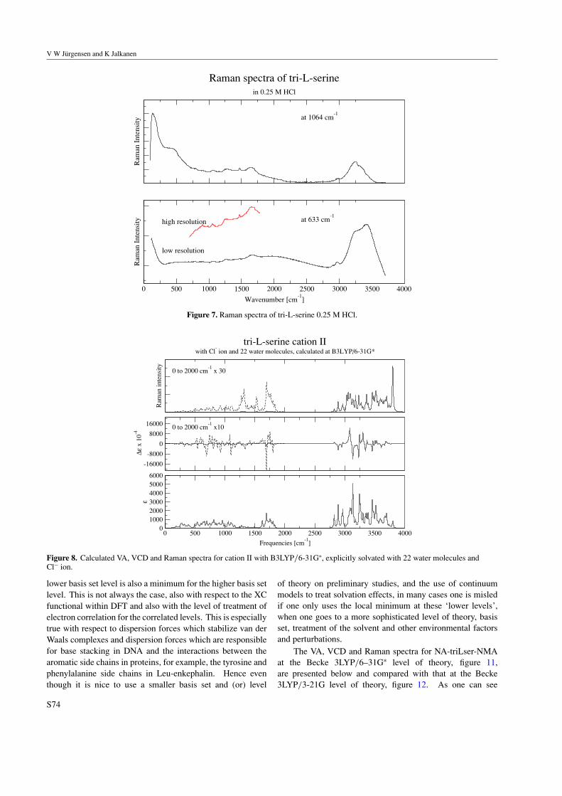
V W Jurgensen and K Jalkanen
Ram
an I
nten
sity
Raman spectra of tri-L-serinein 0.25 M HCl
0 500 1000 1500 2000 2500 3000 3500 4000
Wavenumber [cm-1
]
Ram
an I
nten
sity
at 1064 cm-1
at 633 cm-1
high resolution
low resolution
Figure 7. Raman spectra of tri-L-serine 0.25 M HCl.
Ram
an in
tens
ity
tri-L-serine cation IIwith Cl
- ion and 22 water molecules, calculated at B3LYP/6-31G*
-16000
-8000
0
8000
16000
∆ε x
10-4
0 500 1000 1500 2000 2500 3000 3500 4000
Frequencies [cm-1
]
0100020003000400050006000
ε
0 to 2000 cm-1
x 30
0 to 2000 cm-1
x10
Figure 8. Calculated VA, VCD and Raman spectra for cation II with B3LYP/6-31G∗, explicitly solvated with 22 water molecules andCl− ion.
lower basis set level is also a minimum for the higher basis setlevel. This is not always the case, also with respect to the XCfunctional within DFT and also with the level of treatment ofelectron correlation for the correlated levels. This is especiallytrue with respect to dispersion forces which stabilize van derWaals complexes and dispersion forces which are responsiblefor base stacking in DNA and the interactions between thearomatic side chains in proteins, for example, the tyrosine andphenylalanine side chains in Leu-enkephalin. Hence eventhough it is nice to use a smaller basis set and (or) level
of theory on preliminary studies, and the use of continuummodels to treat solvation effects, in many cases one is misledif one only uses the local minimum at these ‘lower levels’,when one goes to a more sophisticated level of theory, basisset, treatment of the solvent and other environmental factorsand perturbations.
The VA, VCD and Raman spectra for NA-triLser-NMAat the Becke 3LYP/6–31G∗ level of theory, figure 11,are presented below and compared with that at the Becke3LYP/3-21G level of theory, figure 12. As one can see
S74

The VA, VCD, Raman and ROA spectra of tri-L-serine in aqueous solution
Ram
an in
tens
ities
-40000
-20000
0
20000
40000
∆ε x
10-4
0 1000 2000 3000 4000
Frequency [cm-1
]
0100020003000400050006000
ε
0 to 2000 cm-1
x 20
Mid IR times 30
tri-L-serine cation II
with Cl- ion and 22 water molecules, calculated at B3LYP/6-31G* with Onsager
Figure 9. Calculated VA, VCD and Raman spectra for cation II with B3LYP/6-31G∗, explicitly solvated with 22 water molecules and aCl− ion, within Onsager solvation sphere (except AAT).
Ram
an in
tens
ities
-30000
-15000
0
15000
30000
∆ε x
10-4
0 500 1000 1500 2000 2500 3000 3500 4000
Frequency [cm-1
]
0
1000
2000
3000
4000
5000
ε
0 to 2000 cm-1
x 30
Mid IR times 30
tri-L-serine cation II
with Cl- ion and 22 water molecules, calculated at B3LYP/6-31G* level, Onsager geom
Figure 10. Calculated VA, VCD and Raman spectra for cation II calculated at B3LYP/6-31G∗, explicitly solvated with 22 water moleculesand a Cl− ion, geometry optimized within Onsager solvation sphere (i.e. AAT, Hessian, APT and EDEDPD calculated without).
Table 2. Torsional angles for NALSLSLSNMA at Becke 3LYP level with the 6-31G∗ and 3-21G basis sets.
B3LYP φ1 ψ1 χ 1,1 χ 1,2 ω1 φ2 ψ2 χ 2,1 χ 2,2 ω2 φ3 ψ3 χ 3,1 χ 3,2
3-21G −171 179 176 −100 158 −96 179 180 −100 158 −104 −170 −169 −1786-31G∗ −157 169 −180 −91 159 −82 170 −176 −91 160 −96 −171 −167 −176
there are very large differences in the VA, VCD and Ramanspectra using the Becke 3LYP hybrid XC functional and thetwo different basis sets. Hence it is clear that the 3-21Glevel of theory which has been advocated for simple organiccompounds, does not appear to be adequate to represent
peptide systems. Also shown are the ROA spectra for theNA-triLser-NMA with the Becke 3LYP hybrid XC functionaland 6–31G∗ and 3-21G basis sets, figure 13. We presentthe simulated results for the ROA spectra to document thefeasibility of these calculations and also to show how the
S75
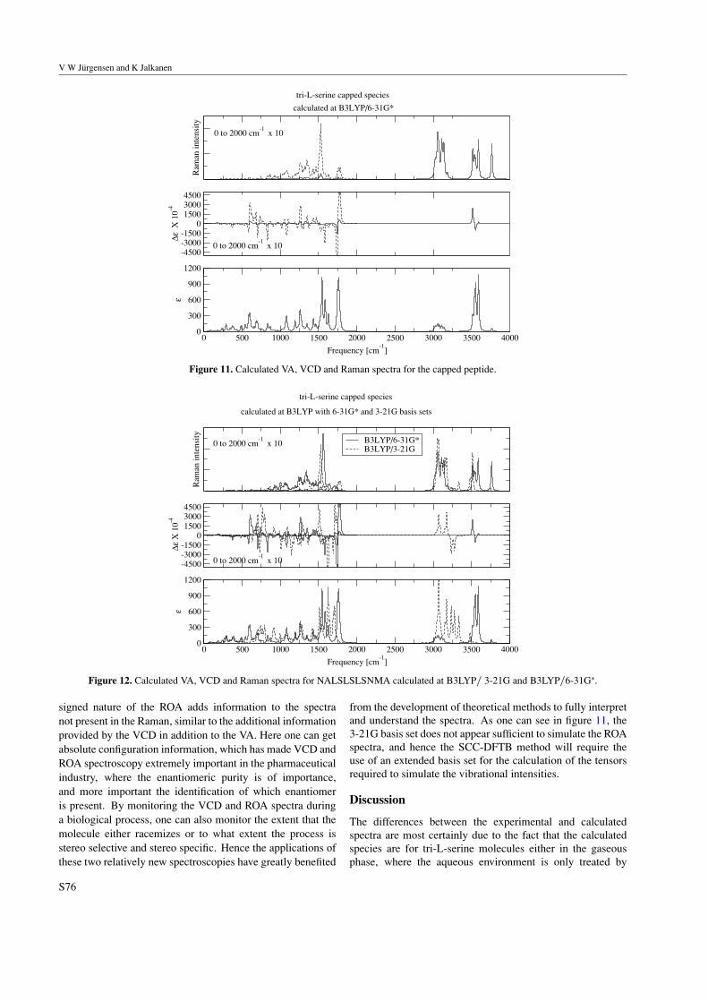
V W Jurgensen and K Jalkanen
Ram
an in
tens
ity
-4500-3000-1500
0150030004500
∆ε X
10-4
0 500 1000 1500 2000 2500 3000 3500 4000
Frequency [cm-1
]
0
300
600
900
1200
ε
0 to 2000 cm-1
x 10
0 to 2000 cm-1
x 10
tri-L-serine capped species
calculated at B3LYP/6-31G*
Figure 11. Calculated VA, VCD and Raman spectra for the capped peptide.
Ram
an in
tens
ity
-4500-3000-1500
0150030004500
∆ε X
10-4
B3LYP/6-31G*B3LYP/3-21G
0 500 1000 1500 2000 2500 3000 3500 4000
Frequency [cm-1
]
0
300
600
900
1200
ε
0 to 2000 cm-1
x 10
0 to 2000 cm-1
x 10
tri-L-serine capped species
calculated at B3LYP with 6-31G* and 3-21G basis sets
Figure 12. Calculated VA, VCD and Raman spectra for NALSLSLSNMA calculated at B3LYP/ 3-21G and B3LYP/6-31G∗.
signed nature of the ROA adds information to the spectranot present in the Raman, similar to the additional informationprovided by the VCD in addition to the VA. Here one can getabsolute configuration information, which has made VCD andROA spectroscopy extremely important in the pharmaceuticalindustry, where the enantiomeric purity is of importance,and more important the identification of which enantiomeris present. By monitoring the VCD and ROA spectra duringa biological process, one can also monitor the extent that themolecule either racemizes or to what extent the process isstereo selective and stereo specific. Hence the applications ofthese two relatively new spectroscopies have greatly benefited
from the development of theoretical methods to fully interpretand understand the spectra. As one can see in figure 11, the3-21G basis set does not appear sufficient to simulate the ROAspectra, and hence the SCC-DFTB method will require theuse of an extended basis set for the calculation of the tensorsrequired to simulate the vibrational intensities.
Discussion
The differences between the experimental and calculatedspectra are most certainly due to the fact that the calculatedspecies are for tri-L-serine molecules either in the gaseousphase, where the aqueous environment is only treated by
S76

The VA, VCD, Raman and ROA spectra of tri-L-serine in aqueous solution
-3000-2000-1000
0100020003000
RO
A in
tens
ity
-3000-2000-1000
0100020003000
RO
A in
tens
ityB3LYP/3-21GB3LYP/6-31G
0 500 1000 1500 2000 2500 3000 3500 4000
Frequency [cm-1
]
-3000-2000-1000
0100020003000
RO
A in
tens
itiy CID1
CID2
CID3
tri-L-serine capped species
B3LYP/6-31G* and B3LYP/3-21G
Figure 13. Calculated ROA spectra for NALSLSLSNMA calculated at B3LYP/3-21G and B3LYP/6-31G∗.
continuum models, where we only treat a small number ofthe water molecules, or where we combine the small clusterof explicit water molecules hydrogen bonded to tri-L-serinewith the continuum solvent models. Even though the solventmedium of the species is simulated with either the Onsageror PCM continuum models, this cannot be regarded as inaqueous solution, since strong solvent interaction from theside-chain serine groups is expected but not considered atall with the continuum solvent models. Another possibilityfor the discrepancies between experiment and calculations,which is equally important, is the fact that the spectra arenot calculated at a global energy minimum, as we know of,since no systematic energy minimization was done. We havetried to improve upon the gas phase and continuum modelsby including the explicit water molecules which are hydrogenbonded with the cationic species and also which solvate theCl− anion. This clearly treats the direct interactions muchbetter than the two continuum models, but does not treat theeffects due to bulk water. Hence we have embedded our tri-L-serine cation plus the Cl− anion within the two cavities, eitherspherical in the case of the Onsager model, or shape of thecluster in the case of the PCM model. This clearly appears theway to go. Since the point of this work was to documentthe various ways to treat the effects due to the aqueousenvironment, counterions and pH on both the structural andvibrational properties, we feel we have accomplished that withour last set of calculations. A future publication shall presentour results at this level of theory for all species and also performa systematic potential energy surface (PES) at this level oftheory. This will require a lot of computer time and hence theprograms which we have used must also be very efficient to beable to do this. Hence we are also in the process of modifyingthe programs to make such calculations feasible for not onlytripeptide systems, but also much larger peptide systems. Thisis clearly also a criterion if we wish to perform the required
sampling and averaging required to simulate the VA, VCD,Raman and ROA spectra for all species and conformers forbiological molecules, here peptides in solution and bound toproteins.
For the experimentally obtained VCD spectrum it canbe said, other than features between VA and VCD spectracoincide, that the region around 1700 wave numbers almostexhibits the same ±/+ pattern as the calculated spectrum.
Eker et al have presented a combined Raman, VA andVCD study of tripeptides in aqueous solution, similar to ourprevious works on LA, NALANMA and LALA [8, 9, 50]. Intheir study they also present the results for the anionic speciesof tri-L-serine. This was the only species for tri-L-serine forwhich they were able to obtain the backbone torsion angle(φ1,ψ1) and (φ2,ψ2). Their reported values were (–135, 178)and (–175, 135), respectively. They found a very large pDdependence of the VA, VCD and Raman spectra for tri-L-serine, much larger than for the other tripeptides studied. Thisis not surprising due to the nature of the side chains of tri-L-serine, all being OH groups, which allow for both hydrogenbonding and protonation. Here the explicit water model andour hybrid explicit water model combined with the continuumsolvent models are very applicable. The results we have todate suggest that our model should be able to answer theoutstanding questions left unanswered in the study of Ekeret al. In a future publication, we will present our complete setof results from our hybrid for the complete set of the speciesfor tri-L-serine, which is beyond the scope of this work.
In the article of Eker et al the amide I bands of severalspecies were measured, but due to purely signal to noise issues,only the spectra of the anionic species were presented. A quickcomparison between our calculated and their measured spectrashows that our calculated amide I band is shifted towardshigher wave numbers, around 1700–1790 cm−1, while themeasured values lay a little bit lower around 1630–1730 cm−1.
S77

V W Jurgensen and K Jalkanen
Hence, our experimental peaks are closer to the experimentalresults of Eker et al, which lie around 1650 cm−1 [51]. Theoverall features are very hard to compare, but do not seemsimilar, except for the lower frequency peak being higher inintensity than the next. Our calculated VCD spectra, thoughagain shifted towards higher wave numbers, seem to show theoverall features of their measured VCD spectrum for the acidicspecies rather than the alkaline.
Conclusions and outlook
In this work, we have utilized the B3LYP DFT level oftheory to model various species of tri-L-ser and NA tri-L-serNMA. In this work, we have added explicit water molecules,and have also tested the ability or capabilities of one ofthe newly developed continuum models, the so-called PCMmodel. Previously, the Onsager continuum has been shownto be inadequate to treat amino acids and small peptides dueto its not taking into account the specific hydrogen bondedinteractions. This also appears to be the case for the PCMmodel. Even the developers of this model have come to similarconclusions on other simpler systems. But this level of theoryneeds to be further tested on larger systems such as the twopresented here, that is, tri-L-serine and NA tri-L-ser NMA.It appears that even for larger peptides and capped peptides,the inclusion of explicit water molecules to treat the watermolecules in the first hydration shell that directly interact withthe polar parts of the molecule is extremely important. Thetreatment of these waters is important for many reasons. Firstlyif they are not included, the structures with intermolecularhydrogen bonds are almost always lowest in energy due to thestabilization energy generated by these interactions. But inaqueous solution it is the total energy of the whole system,which must be a minimum and not just the lowest energyof the individual parts. Hence the cooperativity effects andsynergistic interactions must be treated. The hope is that onlythe strongly hydrogen bonded interactions are necessary forthese calculations, but the definitive answer to this questionis still open and we are still working on this problem in thissystem and others, where we hope to be able to develop anautomated way of answering this question. In addition, thestructures that include the explicit water molecules are in manycases not even local minimum on the PES for the isolatedmolecule, so one has no chance of even finding them withoutexplicitly adding waters. Also if one wishes to simulate theVA, VCD, Raman and ROA spectra, as is our goal, then oneneeds not only to find the correct local minimum for the peptide+ N explicit water molecules but also to treat the coupling ofthe modes of the solvent with the water molecules in this localhydration shell environment. The process of energy transfer,redistribution and charge transfer are also very important inunderstanding the function of biomolecules, so these are alsogoals of our studies, we not only want the structure, as manystudies do, but we want the VA, VCD, Raman and ROAspectra and the electric, magnetic and nuclear properties ofthe molecule and its hydration shell, since they are also veryimportant for our goal of understanding the structure andfunction of biomolecules via probing with electromagneticradiation in the various environments where the molecules
are present in their native states, but also under non-nativeconditions which may arise and which may for instance beresponsible for illness. Hence the goal is to be able tounderstand medicine at a molecular level, and here one requiresnot only just the structures of the various molecules in aqueoussolution, but also their interactions with each other, with thesolvent and ultimately as a function of the environmentalstresses which cause illnesses, so that we can develop possiblesafeguards and cures.
Acknowledgments
The Danish Research Council is acknowledged for its financialsupport for the Quantum Protein Centre and VWJ’s PhDstipendium (grant). The authors would like to thankJ Sonne, T H Pedersen (QuP-Centre) for their part in thecalculations and H H Drews from Brucker Optik GMBH, FT-IR applications Marketing, Rudolf-Plank-Str. 23, D-76275Ettlingen, Germany for the help with the experimentalmeasurements, as well as other staff members. We would alsolike to thank the German Cancer Research Center (the DKFZ)in Heidelberg, Germany for providing computer resources,which allowed the large solvated systems to be calculatedon the HP Cluster at the DKFZ. In addition, we would like tothank the staff at Thermo Electron, Madison, WI, USA for helpwith the Raman measurements. We would also like to thankthe Laboratory of Physics at Helsinki University of Technologyand the Finnish Academy of Science for supporting thisresearch project during KJJ’s many visits to the Laboratory ofPhysics and for the fruitful discussions with Risto Nieminenand Ivan Degtyarenko. In addition, KJJ would like to thankJulian Gale for fruitful discussions and the Government ofWestern Australia for funding under the Premier Researchfellow program.
References
[1] Onsager L 1936 J. Am. Chem. Soc. 58 1486–93[2] Gill P M W Density functional theory (DFT) Hartree–Fock
(HF) and Self-consistent Field in Encyclopedia ofComputational Chemistry (New York: Wiley) pp 678–88
[3] Frisch M J et al 2001 (Pittsburgh, PA: Gaussian Inc.)Gaussian 98 and 2003
[4] Atkins P W and Friedman R S 2004 Molecular QuantumMechanics 4th edn (Oxford: Oxford University Press)
[5] Kohn W 1999 Rev. Mod. Phys. 71 1253–66[6] Jalkanen K J, Bohr H G and Suhai S 1997 Density functional
and neural network analysis: hydration effects andspectroscopic and structural correlations in small peptidesand amino acids Theoretical and Computational Methods inGenome Research ed S Suhai (New York: Plenum)pp 255–77
[7] Jensen F 1999 Introduction to Computational Chemistry (NewYork: Wiley)
[8] Jalkanen K J, Nieminen R M and Bohr J 2000 Simulations andanalysis of the Raman scattering and differential Ramanscattering/Raman optical activity (ROA) spectra of aminoacids, peptides and proteins in aqueous solutionVestn. Mosk. Univ. Khim. 41 4–7
S78

The VA, VCD, Raman and ROA spectra of tri-L-serine in aqueous solution
Jalkanen K J, Nieminen R M, Frimand K, Bohr J, Bohr H,Wade R C, Tajkhorshid E and Suhai S 2001 Chem.Phys. 265 125–51
Tajkhorshid E, Jalkanen K J and Suhai S 1998 J. Phys. Chem.B 102 5899–913
Frimand K, Bohr K, Jalkanen K J and Suhai S 2000Chem. Phys. 255 165–94
[9] Han W G, Jalkanen K J, Elstner M and Suhai S 1998 J. Phys.Chem. B 102 2587–602
[10] Jalkanen K J and Suhai S 1996 N-acetyl-L-alanineN′-methylamide: a density functional analysis of thevibrational absorption and vibrational cirkular dichroismspectra Chem. Phys. 208 81–116
Deng Z, Polavarapu P L, Ford S J, Hecht L, Barron L D,Ewig C and Jalkanen K J 1996 J. Phys. Chem.100 2025–34
[11] Jalkanen K J, Jurgensen V W and Degtyarenko I M 2005Adv. Quantum Chem. 50 91–124
[12] Bohr H, Jalkanen K J, Elstner M, Frimand K and Suhai S 1999Chem. Phys. 246 13–36
Frimand K and Jalkanen K J 2002 Chem. Phys. 279 161–78Abdali S, Niehaus T, Jalkanen K J, Ciao X, Nafie L A,
Frauenheim Th, Suhai S and Bohr H 2003 Phys. Chem.Chem. Phys. 5 1295–300
Jalkanen K J et al 2006 Int. J. Quantum Chem. 106 1160–98[13] Talman J D and Shadwick F W 1976 Phys. Rev. A 14 36–40[14] Hirata S, Ivanov S, Grabowski I, Bartlett R J, Burke K and
Talman J D 2001 J. Chem. Phys. 115 1635–49[15] Krieger J B, Li Y and Infrate G J 1992 Phys. Rev. A45
101–26[16] Yanai T, Tew D P and Handy N C 2004 Chem. Phys.
Lett. 393 51–7[17] Bauernschmitt R and Ahlrichs R 1996 Chem. Phys. Lett.
256 454–64Dreuw A and Head-Gordon M 2004 J. Am. Chem. Soc.
126 4007–16Gritsenko O and Baerends E J 2004 J. Chem. Phys.
121 655–60Tawada Y, Tsuneda T, Yanagisawa S, Yanai T and Hijaro K
2004 J. Chem. Phys. 120 8425–33Hirata S, Ivanov S, Grabowski I and Bartlett R J 2002 J. Chem.
Phys. 116 6468–81Neiss C, Saalfrank P, Parac M and Grimme S 2003 J. Phys.
Chem. A107 140–7[18] Engel E and Bonetti A F 2001 Int. J. Mod. Phys. B 15 1703–13[19] Hirata S, Ivanov S, Bartlett R J and Grabowski I 2005
Phys. Rev. A 71 032507-1-7[20] Onida G, Reining L and Rubio A 2002 Rev. Mod. Phys.
74 601–59Reining L, Olevano V, Rubio A and Onida G 2002 Phys. Rev.
Lett. 88 066404Ismail-Beigi S and Louie S G 2003 Phys. Rev. Lett.
90 076401Zhukov V P, Chulkov E V and Echenique P M 2004 Phys.
Rev. Lett. 93 096401Botti S, Sottile F, Vast N, Olevano V, Reining L,
Weissker H-C, Rubio A, Onida G, Sole R D and Godby RW 2004 Phys. Rev. B 69 155112
[21] Soler J M, Artacho E, Gale J D, Garcia A, Junquera J,Ordejon P and Sanchez-Portal D 2002 J. Phys.: Condens.Matter 14 2745–79
[22] Gonze X et al 2002 Comput. Mater. Sci. 25 468–92[23] Tomasi J, Mennucci B and Cammi R 2005 Chem. Rev.
105 2999–3093Cramer C J and Truhlar D G 1999 Chem. Rev. 99 2161–200
Tomasi J and Persico M 1994 Chem. Rev. 94 2027–94Miertus S, Scrocco E and Tomasi J 1981 Chem. Phys.
55 117–29[24] Poon C-D, Salulski T, Weise C F and Weisshaar J C 2000
J. Am. Chem. Soc. 122 5642–3Weise C F and Weisshar J C 2003 J. Phys. Chem.
B 107 3265–77[25] Sen A C and Keiderling T A 1984 Biopolymers 23 1533–45
Carney J R and Zwier T A 1999 J. Phys. Chem.A 103 9943–57
Mons M, Dimicoli I, Tardivel B, Piuzzi F, Brenner V andMillie P 1999 J. Phys. Chem. A103 9958–65
[26] Diem M, Oboodi M R and Alva C 1984Biopolymers 23 1917–30
[27] Bour P, Kubelka J and Keiderling T A 2002Biopolymers 65 145–59
[28] Stephens P J 1985 J. Phys. Chem. 89 748–52[29] Amos R D, Handy N C, Jalkanen K J and Stephens P J 1987
Chem. Phys. Lett. 133 21–6[30] Stephens P J 1987 J. Phys. Chem. 91 1712–15[31] Buckingham A D 1987 Chem. Phys. 112 1–14[32] Amos R D, Jalkanen K J and Stephens P J 1988 J. Phys.
Chem. 92 5571–75[33] Bak K L, Jørgensen P, Helgaker T, Ruud K and Jensen H J Aa
1993 J. Phys. Chem. 98 8873–87[34] Bak K L, Jørgensen P, Helgaker T, Ruud K and Jensen H J Aa
1994 J. Chem. Phys. 100 6621–27[35] Bak K L, Delvin F J, Ashvar C S, Taylor P R, Frisch M J and
Stephens P J 1995 J. Phys. Chem. 99 14918–22[36] Jalkanen K J, Stephens P J, Amos R D and Handy N C 1988
J. Phys. Chem. 92 1781–5[37] Stephens P J, Jalkanen K J, Amos R D, Lazzeretti P and
Zanasi R 1990 J. Phys. Chem. 94 1811–30[38] Hansen A, Stephens P J and Bouman T D 1991 J. Phys.
Chem. 95 4255–62[39] Bak K L, Hansen A E and Stephens P J 1995 J. Phys.
Chem. 99 17359–63[40] Ditchfield R 1972 J. Chem. Phys. 56 5688–91[41] Epstein S T 1973 J. Chem. Phys. 58 1592–95[42] Ditchfield R 1974 Mol. Phys. 27 789–807[43] Bouman T D and Hansen A E 1988 Chem. Phys.
Lett. 159 510–15[44] Wilkins M R, Gasteiger E, Bairoch A, Sanchez J C,
Williams K L, Appel R D and Hochstrasser D F 1998Calculated by the program primary structure analysis(pI/M.W.) Protein Identification and Analysis Tools in theExPASy Server in: 2-D Proteome Analysis Protocolsed A J Link (New Jersey: Humana Press) on ExPASywww.expasy.org
[45] GaussView a visualization and analysis program fromGaussian Inc. [3]
[46] Schaftenaar G and Noordik J H 2000 Molden: a pre- andpost-processing program for molecular and electronicstructures J. Comput.-Aided Mol. Des. 14 123–34
[47] Schweitzer-Stenner R 2001 J. Raman Spectrosc. 32 711–32[48] Mirkin N G and Krimm S 1991 J. Mol. Struct. 242 143–60[49] Faurskov Nielsen O 1995 Anvendelse af IR, Raman, UV, VIS,
Flourescens, Phosphorescens i Biofysisk Kemi LectureNotes (Copenhagen: HCØ Tryk)
[50] Jalkanen K J, Nieminen R M, Knapp-Mohammady M andSuhai S 2003 Int. J. Quantum Chem. 92 239–59
Knapp-Mohammady M, Jalkanen K J, Nardi F, Wade R C andSuhai S 1999 Chem. Phys. 240 63–77
[51] Eker F, Cao X, Nafie L and Schweitzer-Stenner R 2002 J. Am.Chem. Soc. 124 14330–41
S79