Journal of Energy Systems

2021, 5(2)

2602-2052 DOI: 10.30521/jes.823017 Research Article

121

Numerical approximation of the hydrological time of concentration

Juan Ramón Barrón-Fernández Department of Building, University of Extremadura, Cáceres, Spain, jrbarronf@unex.es

Carmen Calvo-Jurado Department of Mathematics, University of Extremadura, Cáceres, Spain, ccalvo@unex.es

Submitted: 07.11.2020

Accepted: 02.05.2021

Published: 30.06.2021

Abstract: The time of concentration, that is the time it takes for a single "drop of water" to move

superficially from the most distant point of the watershed to the exit point, is a fundamental

parameter of the hydrological analysis. Many studies have been conducted to propose empirical

formulas to calculate the time of concentration. One of the best known is the Temez formula

based on time series data collected in accounts in Spain with areas of less than 3,000 km2. This

expression uses the main channel length as a parameter as in many works, for small slopes is

approximated by the distance between the geographic coordinates between the starting and ending

points, leading for larger catchments and slopes to approaches with a high error. In this work,

using a proper discretization of the curve, by using polynomial interpolation methods, we improve

the calculation of the length of the main channel and therefore, we provide a more reliable method

for calculating the time of concentration using the Temez expression. We illustrate the proposed

scheme with different numerical examples comparing the results with those provided by other

methods.

Keywords: Concentration time, Interpolation methods, Main channel length, Temez’s formula

Cite this paper as: Barrón-Fernández, J.R., Calvo-Jurado, C., Numerical approximation of the hydrological time of

concentration. Journal of Energy Systems 2021, 5(2), 121-136, DOI: 10.30521/jes.823017

© 2021 Published by peer-reviewed open access scientific journal, JES at DergiPark (https://dergipark.org.tr/en/pub/jes)

Journal of Energy Systems

122

1. INTRODUCTION

In hydrological analyses, data and parameters are needed to quantify the variables studied by different

methods and models. An important and difficult parameter to study due to its variability is the

concentration time (i.e. 𝑇𝑐) [1,2]. According to some authors, the time of concentration can be defined

as the time that a single drop of water takes to travel from the most distant point in the basins to the

point of exit [3-8]. Following [3], this parameter is related to the lines of equal time of flow to the outlet,

called isochrones representing the grown of contributing area to the streamflow outlet after certain time.

The time at which all of the watershed begins to contribute is 𝑇𝑐 (see in Fig. 1). Johnstone and Cross

[4] present three main problems of stream flow: Mean annual flow, drought flow and flood flow. To

solve the problem, they present the main principles involved as the parameter 𝑇𝑐 applied to specific

areas in America (see Eq. (4)). In [5], the accuracy of three popular flood routing models are evaluated

in Canada. They also extend the routing formulations developed by other authors (Kesking and

Agiralioglu). Following Ref. [6], it is checked experimentally that this parameter is characteristic of

each basin and, therefore, regardless of the configuration and magnitudes of the downpour. It is proposed

to calculate by following the expression:

𝑇𝑐 = 0.3 (1.5 𝐿𝑐

0.8√𝐻)

0.76

(1)

where 𝐿𝑐 and H denote the length and the average slope of the river main course respectively. The

Bransby Williams formula for the time of concentration dates from 1922, when Williams published the

work [7]. In this paper, Williams provides the formula (2) for a parameter (nowadays known as time of

concentration) that describes the time taken for the water to reach the point of discharge from the most

distance point of the watershed. This measure is considered after the maximum flood produced by the

greatest possible rainfall. Other works, (see [8]) put forward the hydrological data quality method based

on data-driven methods as an alternative to determine the hydrological data more efficiently and to

provide an accurately reference for the hydrological workstations. 𝑇𝑐 functionality is also defined as the

design of rainwater systems, hydraulic structures using rational methods and operations in hydraulic

infrastructures [9]. There are a variety of empirical equations to calculate this parameter, some of which

are:

Bransby-Williams’s Model [5]:

𝑇𝑐 = 0.2426 𝐿𝑐𝐴−0.1𝑆𝑐−0.2 (2)

Where 𝐿𝑐 denotes the length of main watercourse channel (km); 𝑆𝑐 the average main watercourse slope

and A refers to the catchment area (𝑘𝑚2). The expression Eq. (2) is derived from observations of floods

in rural catchments in the region of India, for areas smaller than 129.50 𝑘𝑚2.

Giandotti’s Model [10]:

𝑇𝑐 = 4√𝐴 +1.5 𝐿𝑐

0.8√𝐻 (3)

where H is difference between the average elevation of the whole catchment area and the outlet section.

This expression developed through the study of twelve large catchment areas in northern and central

Italy, for areas between 170 and 70,000 𝑘𝑚2.

Journal of Energy Systems

123

Kirpich’s Model [11]:

𝑇𝑐 = 0.0663 𝐿𝑐0.77𝑆𝑐

−0.385 (4)

It is deduced from the multiple regression of rainfall time series in small agricultural basins in Tennessee

and Pennsylvania, for areas between 0.004 and 0.453 𝑘𝑚2, and average slope between 3 % and 10 %.

Johnstone and Cross’s Model [4]:

𝑇𝑐 = 0.0543 𝐿𝑐0.5𝑆𝑐

−0.5

(5)

This formula was developed from the study of 19 sub-basins, located in Scioto and Sandysky (Ohio)

area. The area of the basin must be between 65 to 4,206 𝑘𝑚2.

NRCS-SCS Method [2]:

𝑇𝑐 = 0.057 (1,000

𝐶𝑁− 9) 𝐿𝐶

0.8𝑆𝐶−0.5 (6)

Where CN denotes the number of the run-off curve. This expression was developed by Soil Conservation

Service (SCS) which later became Natural Resources Conservation Service (NRCS). It is based on was

based on data collected from homogeneous agricultural catchments with areas of up to 8 𝑘𝑚2.

Chow’s Model [12]:

𝑇𝑐 = 0.1602 𝐿𝑐0.64𝑆𝑐

−0.32 (7)

This equation was deduced for twenty rural catchments in the U.S. whose area varies from 0.01 to 18.5

𝑘𝑚2, and average slope from 0.0051 to 0.09.

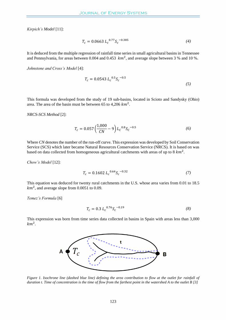
Temez’s Formula [6]

𝑇𝑐 = 0.3 𝐿𝑐0.76𝑆𝑐

−0.19 (8)

This expression was born from time series data collected in basins in Spain with areas less than 3,000

𝑘𝑚2.

Figure 1. Isochrone line (dashed blue line) defining the area contribution to flow at the outlet for rainfall of

duration t. Time of concentration is the time of flow from the farthest point in the watershed A to the outlet B [3]

Journal of Energy Systems

124

Eqs. (2-8) have as a common parameter, the average slope of the main channel 𝑆𝑐 or the points of highest

and lowest elevation of the basin area H. In all of them, it is calculated in the same way for small basins

as for large basins [3, 10, 2, 4, 11, 13, 14, 5, 15, 9, 6, 16, 7].

It is currently possible to determine the characteristics of the basin with great precision thanks to the

large number of data provided the new technologies [17]. Specifically, and mainly due to the systems

of geographic information (GIS) and spatial data infrastructure (IDEE). The GISs are software that allow

applying a multitude of algorithms to raster maps and vector, and IDEE is an infrastructure where data,

metadata, services and information of a geographic type are produced. However, as far as these authors

know, once the data that describe the basin, the calculation of the mean slope is usually carried out by

the methods are not very precise and even depend on the area of the planet and its extension of the basin

where it is applied. In fact, it is usual that in small basins the average slope is approximated through the

geographic coordinates between the starting point and the end point [18]. However, the slope is very

changeable along the riverbed for large basins, and thereby these methods and particularly Temez’s

formula produces large errors in the calculations of large basins. Young rivers located at mountainous

riverbeds with large slopes and a V-shaped cross section are irregular. Mature rivers have low slopes.

Old rivers have very low slopes and no rapids or falls [1]. For all these different characteristics, the

different methods developed to obtain the average slope are not precise. Better results can be found in

[19], where an equivalent hydraulic profile is built from the conversion of parameters fluvial (altitude,

longitude) to the unit.

Therefore, new reliable method for calculating 𝑆𝑐 must be developed. In this sense, the main objective

of this study is to propose another method to determine the mean slope with a greater accurate than the

current ones. Using spatial data infrastructures and proposing a new mathematical model that is

independent of the contour and the size of the basin one and of the area where it is located. We will

illustrate its implementation by applying it to two real cases in the region of Cáceres in Spain.

2. MATERIAL AND METHODOLOGY

In order to determine the parameter 𝑆𝑐 and therefore the concentration time, different methods are

proposed in the literature. In [20], authors estimate 𝑆𝑐 as follows:

𝑆𝑐=𝐻

𝐿 (9)

Figure 2. Approximation of the average slope parameter proposed in Ref. [9].

where L’ is approximated by the main channel length. Fig. 2 shows how in [9] the authors approaches

the distance between any point of the main channel and the control point. Indeed they assume that the

slope is enough small to consider L’=L cos ~L which does not have to happen especially in large and

irregular basins. Therefore, our aim in this section is to propose a more accurate method based on the

approximation of L by using different interpolation methods. For this, in a first step, we need a discrete

approximation of the terrain main channel orography using proper software.

Journal of Energy Systems

125

2.1 GvSIG software

The GvSIG software (v2.5.0.2930) is a geographic information system (GIS) based on free software, a

project promoted by the Valencian Community (Spain). Firstly, the cartography was downloaded from

the spatial data infrastructure (SDI), which was: National Plan of Aerial Orthophotography (PNOA) and

Digital Terrain Model with a 25 meters mesh pitch (MDT25), of the study area. The layers were loaded

in GvSIG and several geoprocesses were performed in the MDT25 layer. The first geoprocessing done

to the layer was "depressions removal", followed by "flow accumulation", "drainage network". At this

point, the PNOA layer was visualized to obtain the control point through a script called "coordinate

capture". In the MDT25 layer, the geoprocess "catchment through the control point" was executed. The

PNOA layer was reloaded and with the mentioned script a new starting coordinate of the main river was

obtained. In the MDT25 layer, the "contour according to flow line" geoprocess was executed to obtain

a table with the coordinates of the points (x,y), the elevation (z), the horizontal distance between the

points (dh) and the real distance between the points (dr).

1.2 Numerical modelling of the channel

GvSIG has provides a set of n+1 geographical Cartesian coordinates D = {(xi, yi, zi)}i=0n where zi

represent the altitude or height in meters from the ground of a place located at the position (xi, yi),

i=0,…n. Table 1 shows the values of orthogonal projection on the x-z plane of the set D. Considering

it, the path of the main channel can be approximated by a polynomial P of degree n.

Table 1. Channel riverbed contour values

X 𝑥0 𝑥1 … 𝑥𝑛

Z 𝑧0 𝑧1 … 𝑧𝑛

In the following, we will approximate the mean slope as the mean of the channel slopes in each

subinterval, i.e.:

𝑆𝑐=∑ 𝑃′(𝑐𝑖)𝑛

1

𝑛 where 𝑐𝑖 =

𝑥𝑖 + 𝑥𝑖+1

2, i=0, 1, …., n (10)

In what follows, for simplicity, we will rename the 𝑧𝑖 coordinates as 𝑦𝑖.

The use in this work of polynomic expressions of the form,

𝑃𝑛 (𝑥) = 𝑎𝑛 𝑥𝑛 + 𝑎𝑛−1 𝑥𝑛−1 + ⋯ + 𝑎2 𝑥2 + 𝑎1𝑥 + 𝑎0,

𝑎𝑖 ∈ 𝑅, 𝑖 = 0, ,1, … , 𝑛

(11)

for the approximation of the watershed, it is due to the simplicity of the calculation of the derivative in

order to derive the mean of the slopes as is described in Eq. (10). In this sense we have the following

uniqueness and existence result.

Theorem 2.1. Given a support of n + 1 different points 𝑆 = {𝑥0 , 𝑥1, … , 𝑥𝑛} and the table of values

given by Table 1, there exists a unique polynomial (given by Eq. (10)) of degree less or equal as n, 𝑃𝑛 ∈𝑃[𝑅] such that 𝑃𝑛 (𝑥𝑖) = 𝑦𝑖 , 𝑖 = 0, 1, … , 𝑛, where 𝑃𝑛[𝑅] denotes the set of all the polynomial functions

with degree less or equal to n.

Contrary to what might be though, these kinds of approximations do not improve the accurate by taking

large number of points in a same interval. The well - known Runge phenomenon occurs: The

interpolation error is less in the central zone of the interval and greater in the extremes. From the

numerical point of view, it is preferable, instead of generating a single interpolating polynomial based

Journal of Energy Systems

126

on many points of an interval, to divide the interval into others so that by means of several polynomials

we will improve the precision in the interpolation. It is a classic problem that was solved by Chebychev

in terms of a family of polynomials known as polynomials by Chebychev. However, it will not be

considered in this work because support nodes are already given by GvSIG. Instead, we will use the

interpolation piecewise polynomial. The piecewise polynomial interpolation consists of dividing the

interval of starting in subintervals and using in each of them polynomials of degree relatively low, trying

that the constructed function defined in pieces approximates the phenomenon we are considering. The

simplest examples are the pieces constant functions and the polygonal (join the points by segments to

get a polygonal) that interpolate only values associated with the nodes. But for the piecewise constants

we cannot demand continuity and for polygonal we cannot demand derivability at the ends of the

subintervals (the interpolating function is not "smooth"). However, in our case the physical conditions

of the problem require smoothness, so that the function that approximates must be differentiable with

continuity. For all these reasons, the more common piecewise polynomial approximation uses

polynomials of degree three and is called interpolation by cubic splines.

In general, piecewise polynomial interpolation can be defined as follows.

Definition 2.2. Let 𝑃 = {a = x0 < x1 … < xn = b} be a partition of the interval [𝑎, 𝑏] , where

we denote 𝐼𝑖 = [𝑥𝑖 , 𝑥𝑖+1], 𝑖 = 0, … , 𝑛 − 1. A spline is a polynomial function piece in each of the 𝐼𝑖

intervals of the partition. We will denote by 𝑆𝑚(𝑃) the set of functions of class 𝑚 − 1 that are piecewise

polynomials of degree 𝑚 in each of the intervals of the partition:

𝑆𝑚(𝑃) = {𝑠𝑖 ∈ 𝐶𝑚−1([𝑎, 𝑏]): 𝑠𝑖|𝐼𝑖∈ 𝑃𝑚[𝑅]} (12)

For example, a spline of degree 3 is a function 𝑆3(𝑥) ∈ 𝐶2([𝑎, 𝑏]) satisfying the following conditions

• 𝑆3|𝐼𝑖= 𝑡𝑖 ∈ 𝑃3[𝑅], 𝑖 = 0, … , 𝑛 − 1.

• 𝑆3(𝑥𝑖) = 𝑦𝑖, 𝑖 = 0, … , 𝑛.

• 𝑆3 verifies the following conditions in the interval [𝑎, 𝑏].

⋄ 𝑆3′(𝑎) = 𝑓′(𝑎), 𝑆3′(𝑏) = 𝑓′(𝑏) (𝑓𝑖𝑥𝑒𝑑 𝑠𝑝𝑙𝑖𝑛𝑒).

⋄ 𝑆3′′(𝑎) = 𝑆3′′(𝑏) = 0 (𝑛𝑎𝑡𝑢𝑟𝑎𝑙 𝑠𝑝𝑙𝑖𝑛𝑒)

⋄ 𝑆3′(𝑎) = 𝑆3′(𝑏) = 0 𝑎𝑛𝑑 𝑆3′′(𝑎) = 𝑆3′′(𝑏) (𝑝𝑒𝑟𝑖𝑜𝑑𝑖𝑐 𝑠𝑝𝑙𝑖𝑛𝑒).

(13)

In order to obtain 𝑆3(𝑥) observe that ∀𝑖 = 0, … , 𝑛 − 1, 𝑆3 ∈ 𝑃3[𝑅] and therefore it is given by 4

coefficients.

𝑠𝑖(𝑥) = 𝑎𝑖 + 𝑏𝑖(𝑥 − 𝑥𝑖) + 𝑐𝑖(𝑥 − 𝑥𝑖)2 + 𝑑𝑖(𝑥 − 𝑥𝑖)3. (14)

As there are 𝑛 subintervals, it is necessary to determine 4𝑛 constants. On the other hand, we have

• 𝑛 + 1 interpolation conditions:

𝑠𝑖(𝑥𝑖) = 𝑦𝑖 , 𝑖 = 0, … , 𝑛 − 1, 𝑠𝑛−1(𝑥𝑛) = 𝑦𝑛. (15)

• 3(𝑛 − 1) conditions by imposing 𝑆3(𝑥) ∈ 𝐶2([𝑎, 𝑏]).

𝑠𝑖(𝑥𝑖+1) = 𝑠𝑖+1(𝑥𝑖+1), 𝑖 = 0, … , 𝑛 − 2.

𝑠′𝑖(𝑥𝑖+1) = 𝑠′𝑖+1(𝑥𝑖+1), 𝑖 = 0, … , 𝑛 − 2.

𝑠′′𝑖(𝑥𝑖+1) = 𝑠′′𝑖+1(𝑥𝑖+1), 𝑖 = 0, … , 𝑛 − 2.

(16)

Journal of Energy Systems

127

Shortly, we have (𝑛 + 1) + 3(𝑛 − 1) = 4𝑛 − 2 equations to determine 4𝑛 unknowns. So, we need to

consider two additional conditions in order to verify the spline uniqueness. These conditions are

followed from Eqs. (12-13).

For a detailed idea of the effective calculation of cubic splines we refer to Theorem 3.11 in Ref. [12].

Analogously, splines of degree 2 and 1 can be determine.

3. RESULTS

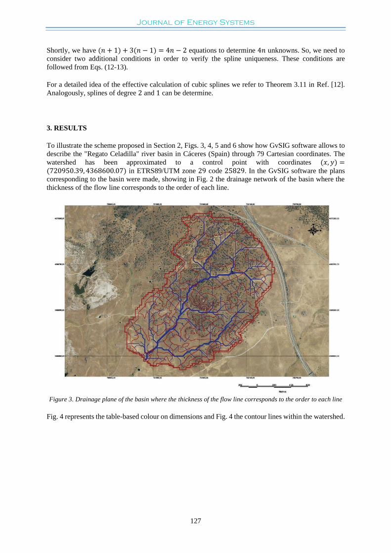
To illustrate the scheme proposed in Section 2, Figs. 3, 4, 5 and 6 show how GvSIG software allows to

describe the "Regato Celadilla" river basin in Cáceres (Spain) through 79 Cartesian coordinates. The

watershed has been approximated to a control point with coordinates (𝑥, 𝑦) =(720950.39, 4368600.07) in ETRS89/UTM zone 29 code 25829. In the GvSIG software the plans

corresponding to the basin were made, showing in Fig. 2 the drainage network of the basin where the

thickness of the flow line corresponds to the order of each line.

Figure 3. Drainage plane of the basin where the thickness of the flow line corresponds to the order to each line

Fig. 4 represents the table-based colour on dimensions and Fig. 4 the contour lines within the watershed.

Journal of Energy Systems

128

Figure 4. Hypsometric map of “Regato Celadilla” watershed (Cáceres, Spain)

Figure 5. Map of the “Regato Celadilla” watershed (Cáceres, Spain), contour lines with river drainage network

Journal of Energy Systems

129

Fig. 6 (Fig. 7 (on the left) describes the selected points with coordinates (𝑥, 𝑦) for calculating the

average slope of the main riverbed.

Figure 6. Map of the "Regato Celadilla" river basin (Cáceres, Spain), points for calculating the average slope of

the main riverbed.

Fig. 6 shows that the Lagrange polynomial interpolation constructs a 78 degree polynomial that does

not provides a good approximation of the riverbed at the extreme points of the interval.

𝑃 = 418.831  − 2.699784037494087 × 1016𝑥 + 5.642748677181165 × 1015𝑥2

− 5.408136737963023 × 1014𝑥3 + 3.194622101925719 × 1013𝑥4

− 8.665166556017677 × 10−199𝑥76

− 2.047792108557352 × 10−203𝑥77

+ 2.376944085604347 × 10−208𝑥78

(17)

Figure 6. Lagrange interpolation polynomial approximates the 79 data obtained with GvSIG given by Eq. (17)

Journal of Energy Systems

130

As consequence, it is necessary to provide better approximations of the set of data. In this sense we

construct P by using pieces polynomial interpolation, of first, second and third degree (𝑆𝑘, 𝑘 = 1, 2 ,3).

Following Definition 2.2, we will denote 𝑆𝑘 by the set of all the k-differentiable functions that are k-

degree pieces polynomials 𝑠𝑖 given by Eq. (14) in each of the partition intervals.

By imposing the interpolation and differentiability conditions Eqs. (15-16) at the ends of the

subintervals, some 78 polynomials of degree 1, 2 and 3 are obtained.

𝑆1 = {𝑠1 = 418.831 − 0.0239079𝑥, 𝑠2 = 418.229, 𝑠3 = 418.229 − 0.0281714(−27.063 + 𝑥), … , 𝑠78 = 383.633 − 0.00548643(−2279.14 + 𝑥)},

𝑆2 = {𝑠1 = 418.831 − 0.0009494782916457017𝑥2,

𝑠2 = 435.53322304832756 − 1.32662613568924𝑥 + 0.025393375872159698𝑥2,

𝑠3 = 415.36083122632107 + 0.1641466405740309𝑥 − 0.0021492612387162377𝑥2,

… , 𝑠78 = 35243.59637185137 − 30.35137681332042𝑥 + 0.006606066297746681𝑥2},

(18)

𝑆3 = {𝑠1 = 418.831 − 0.0027525639608865877𝑥2 + 0.00007160785024784927𝑥3,

𝑠2 = 431.6293852364462,

𝑠3 = −1.5248274705853295𝑥 + 0.05780452383042911𝑥2 − 0.0007300480643843417𝑥3,… 𝑠78 = −22670.92377768599 + 30.401744113190002𝑥

−0.013359675974951895𝑥2 + 0.000001956363805974555𝑥3}.

(19)

In Fig. 7, one can observe the approximation 𝑆𝑘 obtained by using first and second order splines.

Figure 8. On the left, polygonal connecting the 79 points of the sample. On the right, quadratic splines that

interpolate the sample

In Fig. 9, as we expected, the cubic spline approximation is smoother and accurate than the polygonal

(Fig. 8 on the left) and second order (Fig. 8 on the right) approximations. Figs. 9, 11 and 12 can also be

seen for the detail of the basin contour. Specifically, Fig. 9 represents only 29 points of the sample (on

the left) and their approximation by using a polygonal (on the right). Fig.11 shows the approximation

by using second and third order polynomial splines as well as the tangent lines in several points, showing

how the latter (see also Fig. 12) provides better approximation of the slopes.

Journal of Energy Systems

131

Figure 9. Cubic splines that approximate the points. Note that the curve described by the cubic splines provides

better approximations to the data.

In Table 2, applying expression Eq. (10) to the expressions obtained in Eq. (18) and Eq. (19), once 𝑐𝑖

(midpoints of each interval) have been calculated. The following approximation of the average slope 𝑆𝑐

parameter are found.

Table 2. Values of 𝑆𝑐 using different method.

Splines-order 1 -0.0217733 Splines-order 3 -0.225804

Splines-order 2 -0.0225509 Temez’s method -0.0215457

Figure 10. On the left, plot of a subset of the sample (29 points) where positive slopes can be observed in the

interval [𝑥21,𝑥22]. On the right, approximation through the polygonal curve that joins them.

Figure 11. On the left, approach using quadratic splines. On the right, interpolation using cubic splines. Tangent

lines have been drawn at the midpoints of the subintervals [𝑥7 , 𝑥8], [𝑥11,𝑥12] and [𝑥21,𝑥22] in magenta and black.

Journal of Energy Systems

132

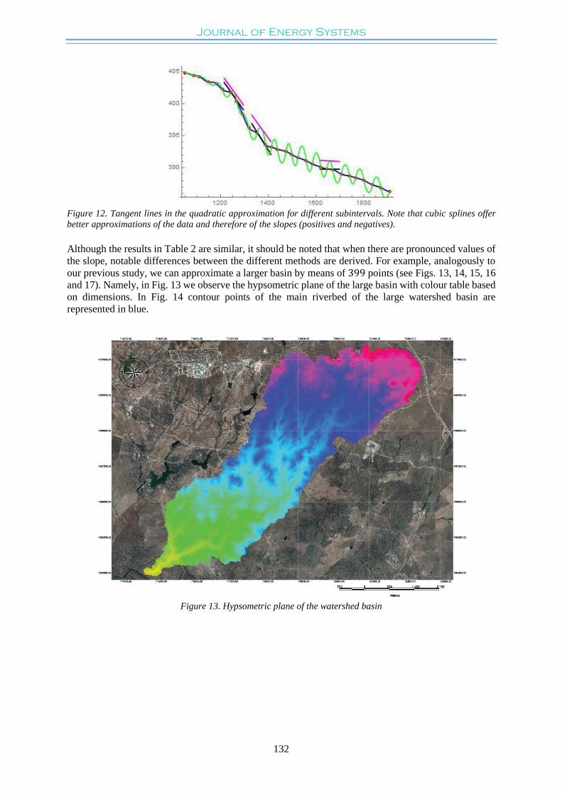
Figure 12. Tangent lines in the quadratic approximation for different subintervals. Note that cubic splines offer

better approximations of the data and therefore of the slopes (positives and negatives).

Although the results in Table 2 are similar, it should be noted that when there are pronounced values of

the slope, notable differences between the different methods are derived. For example, analogously to

our previous study, we can approximate a larger basin by means of 399 points (see Figs. 13, 14, 15, 16

and 17). Namely, in Fig. 13 we observe the hypsometric plane of the large basin with colour table based

on dimensions. In Fig. 14 contour points of the main riverbed of the large watershed basin are

represented in blue.

Figure 13. Hypsometric plane of the watershed basin

Journal of Energy Systems

133

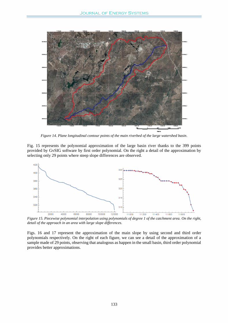
Figure 14. Plane longitudinal contour points of the main riverbed of the large watershed basin.

Fig. 15 represents the polynomial approximation of the large basin river thanks to the 399 points

provided by GvSIG software by first order polynomial. On the right a detail of the approximation by

selecting only 29 points where steep slope differences are observed.

Figure 15. Piecewise polynomial interpolation using polynomials of degree 1 of the catchment area. On the right,

detail of the approach in an area with large slope differences.

Figs. 16 and 17 represent the approximation of the main slope by using second and third order

polynomials respectively. On the right of each figure, we can see a detail of the approximation of a

sample made of 29 points, observing that analogous as happen in the small basin, third order polynomial

provides better approximations.

Journal of Energy Systems

134

Figure 16. Piecewise polynomial interpolation using polynomials of degree 2 of the catchment area. On the right,

detail of the approach in an area with large slope differences.

Figure 17. Piecewise polynomial interpolation using polynomials of degree 3 of the catchment area. On the right,

detail of the approach in an area with large slope differences.

Although Table 3 shows that the overall results for the average slope in the basin are similar taking some

points where the difference in slope is notable, Fig. 7 and Table 4 permit us to observe differences in

the results, showing an imprecise approximation due to Temez's and classical methods.

Table 3. Values of 𝑆𝑐 using different methods

Splines-order 1 -0.018628 Splines-order 3 -0.0194971

Splines-order 2 -0.0191315 Temez method -0.020116

Figure 18. Comparison between Temez methods and those proposed in a watershed area with slope Differences

Table 4. Values of 𝑆𝑐 using different methods

Splines-order 1 -0.0736967 Modified Temez’s method -0.0749217

L 181.567 Temez’s method

-0.0751328

L’ 181.006

Journal of Energy Systems

135

4. CONCLUSION

Although there are different methods in the literature [20, 10, 18, 4, 13, 14, 5, 15, 6, 16, 7] for calculating

the time of concentration and in particular the average slope of the catchment, in general they do not

distinguish between small and large basins. Also, they do not take into account the irregularities of the

slope. In this work we propose a mathematical model based on piecewise polynomial interpolation that

is versatile since it can be used regardless of the size of the basin, the area under study or the variations

in slope. To do it, first a sample of discrete information of the channel contour is obtained using

geographic information system. Using piecewise cubic, quadratic and linear interpolation the riverbed

is approximated. The tangent lines to the splines at the midpoint in each of the subintervals, permit to

obtain a more precise value for the mean slope 𝑆𝑐 than those commonly proposed in the literature. This

allows to determine a more accurate estimation for the time of concentration that constitutes a

fundamental parameter of the hydrological analysis. For small watersheds where there are no large

variations in their slope, the proposed method provides results very similar to the classical models.

However, for large catchment areas or where there are pronounced slope values, the precision of the

method we propose is demonstrated in contrast to the imprecise values of the methods that are commonly

used. In the future, the present work may be improved. For example, the numerical approximation could

consider more hydrological data, such us slope, slope direction or the location of the basin exit point.

For large catchment areas, it would be interesting to take account the local precipitations or regional

seasonal periods. The numerical results would be compared with other predictive models such as other

spatial interpolation methods or statistical control of the data. In particular, the Kriging method would

offer the optimal and unbiased interpolation estimator of spatial distribution values. Also, statistical

control process could help to stablish confidence control of the data according to time series. The

comparison of the conclusions drawn by these methods with the results presented in this work will

provide a detailed estimation of the concentration time regardless of the temporal season, the size and

the location of the watershed.

Acknowledgment

This work has been partially supported through Ministerio de Economía y Competitividad [MTM2017-

83583-P] of Spain and from the Junta de Extremadura through Research Group Grants [GR18023].

REFERENCES

[1] Gracia-Sánchez J, Maza-Álvarez JA. Morfología de Ríos [Rivers morphology]. In: Engineering Institute of the

UNAM eds. Manual de Ingeniería de Ríos. Mexico City, United Mexican States: Series of the Institute of

Engineering Publishing, 1997, pp. 1-46.

[2] Hoeft CC, Humpal A, Cerrelli G. Time of concentration. In: Garrison C, Osenkowsky T, Layer D, Pizzi S,

Hayes W, editors. Hydrology, National Engineering Handbook. Washington DC, United States: U.S.

Department of Agriculture Publishing, 2010, pp: 1-29.

[3] Chow VT, Maidement DR, Mays LW. Applied Hydrology. Singapore, Republic of Singapore: McGraw-Hill,

1988.

[4] Johnstone D, Cross WP. Elements of applied hydrology. New York: Ronald Press Company, 1949.

[5] Perdikaris J, Gharabaghi B, Rudra R. Evaluation of the simplified dynamic wave, diffusion wave and the full

dynamic wave flood routing models. Earth Sciences Research Journal 2018, 7 (2), 14-27, DOI:

10.5539/esr.v7n2p14

[6] Temez JR. Cálculo Hidrometeorológico de Caudales Máximos en Pequeñas Cuencas Naturales

[Hydrometeorological Calculation of Maximum Flows in Small Natural Basins]. Madrid, Spain: Ministry of

Public Works and Urbanism Publising,1978.

[7] Williams GB. Flood discharges and the dimensions of spillways in India. The Engineer 1922, 134 (9), 321 -

322.

[8] Zhao Q, Zhu Y, Wan D, Yu Y, Cheng X. Research on the Data-Driven Quality Control Method of Hydrological

Time Series Data. Water 2018, 10 (12), 1712, DOI: 10.3390/w10121712

[9] Taraglio S, Chiesa S, La Porta, L, Pollino M, Verdecchia M, Tomassetti B, Colaiuda,V, Lombardi A. Decision

support system for smart urban management: resilience against natural phenomena and aerial environmental

Journal of Energy Systems

136

assessment, Int. J. Sust. Energy Planning and Management 2009, 24, 135-146, DOI:

https://doi.org/10.5278/ijsepm.3338

[10] Giandotti M. Previsione dell epiene e dell emagre dei corsid’acqua [Prediction of full and thin water runs].

Roma, Italy: Servizio Idrografico Italiano Publishing, 1934.

[11] Kirpich, ZP. Time of concentration of small agricultural watersheds. Civil Engineering Journal 1940, 10 (6)

362-368.

[12] Burden RL, Faires, JD. Análisis Numérico [Numerical analysis]. Mexico City, United Mexican States: Grupo

Editorial Iberoamérica, 1985.

[13] Martínez G, Díaz JJ. Morfometría en la Cuenca hidrológica de San José del Cabo, Baja California Sur, México

[Morphometry in the hydrological basin of San José del Cabo, Baja California Sur, Mexico]. Revista

Geológica de América Central, 2010, 44, 83-100, DOI: 10.15517/rgac.v0i44.3447

[14] Nagy ED., Torma P, Bene K. Comparing Methods for Computing the Time of Concentration in a Medium-

Sized Hungarian Catchment. JSlovak Journal of Civil Engineering 2017, 24 (4), 8-14, DOI: 10.1515/sjce-

2016-0017

[15] Ravazzani G, Boscarello L, Cislaghi A, Mancini M. Review of Time-of-Concentration Equations and a New

Proposal in Italy. Journal of Hydrologic Engineering, 2019, 24 (10), 04019039, DOI:

10.1061/(ASCE)HE.1943-5584.0001818

[16] Viessman W, Lewis GL. Introduction to Hydrology. Massachusetts, United States of America: Addison-

Wesley Publishing, 1995.

[17] Pusineri G, Pedraza R, Lozeco C. Uso de modelos digitales de elevación y de sistemas de información

geográfica en la modelación hidrológica [Use of digital elevation models and geographic information systems

in hydrological modeling]. Geográfica digital 2005, 2 (3), 1-16, DOI: http://dx.doi.org/10.30972/geo.232664

[18] Grimaldi S, Petroselli A, Tauro F, Porfiri M. Time of concentration: A paradox in modern hydrology.

Hydrological Sciences Journal, 2012, 57 (2) 217-228, https://doi.org/10.1080/02626667.2011.644244

[19] Benavente, MC. Análisis numérico de los perfiles hidrográficos [Numerical analysis of hydrographic

profiles]. Geographical Research Letters 1985, 11, 103-113. DOI: 10.18172/cig.947

[20] Castillo O, Contreras A, Mejías A, Roldán, J, Ruiz, V. Caudal de Referencia, Método Racional Modificado

de Témez. [Reference Flow, Temez's Modified Rational Method]. University of Cádiz, Cádiz, Spain,1991.