numerical experiment to study the modal characteristics … · impulse response in matlab. ......

Dept. of Mech Engg. Amaljyothi College Of Engg.Kanjirapally, Kerala, India

[email protected]

Advanced Dynamics & Control LabDept. of Mech Engg. College of Engineering Trivandrum,

Kerala, India [email protected]

Abstract— In this research work, Euler Bernoulli beam with two degree of freedom per node is used to model a cantilever beam and the governing equations are assembled in the state space form. Rayleigh damping is assumed for computing the impulse response in MATLAB. Transient analysis is performed in ANSYS with newmark beta time integration scheme to obtain the impulse response of Timoshenko beam and are compared with the MATLAB results. The time data from the numerical experiment is transferred to ME’scope modal analysis software and curve fitted in the frequency domain to obtain the FRF of the data. The global curve fitting of the data is done to obtain the frequency, damping and mode shapes.

Keywords—state space; newmark beta; Timoshenko beam; MEScope; curve fitting

I. INTRODUCTION

In the past two decades, modal analysis has become a major technology in the quest for determining, improving and optimizing dynamic characteristics of engineering structures. Not only has it been recognized in mechanical and aeronautical engineering, but modal analysis has also discovered profound applications for civil and building structures, biomechanical problems, space structures, acoustical instruments, transportation and nuclear plants. Modal analysis is the process of determining the inherent dynamic characteristics of a system in forms of natural frequencies, damping factors and mode shapes, and using them to formulate a mathematical model for its dynamic behavior. The formulated mathematical model is referred to as the modal model of the system and the information for the characteristics are known as its modal data. The natural modes of vibration are inherent to a dynamic system and are determined completely by its physical properties (mass, stiffness, damping) and their spatial distributions. Each mode is described in terms of its modal parameters: natural frequency, the modal damping factor and characteristic displacement pattern, namely mode shape. The mode shape may be real or complex. Each corresponds to a natural frequency. The degree of participation of each natural mode in the overall vibration is determined both by properties of the excitation source(s) and by the mode shapes of the system [7].

Modal analysis embraces both theoretical and experimental techniques. The theoretical modal analysis anchors on a physical model of a dynamic system comprising its mass, stiffness and damping properties. These properties may be given in forms of partial differential equations. An example is the wave equation of a uniform vibratory string established from its mass distribution and elasticity properties. The solution of the equation provides the natural frequencies and mode shapes of the string and its forced vibration responses. However, a more realistic physical model will usually comprise the mass, stiffness and damping properties in terms of their spatial distributions, namely the mass, stiffness and damping matrices. These matrices are incorporated into a set of normal differential equations of motion. The superposition principle of a linear dynamic system enables us to transform these equations into a typical eigenvalue problem. Its solution provides the modal data of the system. Modern finite element analysis empowers the discretization of almost any linear dynamic structure and hence has greatly enhanced the capacity and scope of theoretical modal analysis. On the other hand, the rapid development over the last two decades of data acquisition and processing capabilities has given rise to major advances in the experimental realm of the analysis, which has become known as modal testing

II. THEORETICAL BACKGROUND

A. Eigen Values and Eigen Vectors [Ilker Tanyer,2008]Equation of motion in matrix form

0M x K xKK (1)

Multiply the above equation using 1M

1 1 0M M x K M x (2)

0I x C x (3) Where

(4)

International Journal of Scientific & Engineering Research, Volume 5, Issue 7, July-2014 ISSN 2229-5518 747

IJSER © 2015 http://www.ijser.org

IJSER

1M M I

(5) 1K M C

If there are n degrees of freedom, there will be n values of

eigen values)

(6) 2 0I A C A

(7) 2 I A C A

(8) 0I C A

(9) 0I C

This equation gives the values of natural frequencies, once the

value of natural frequencies is known mode shape or eigen

vector can be found out from equation

(10) 0I C A

Where A is the mode shape vector.

B. State Space Representation In order to understand the polyreference frequency

domain method, state-space concept and its applications to vibrational systems must be known. To solve time domain problems using a computer, it is desirable to change the form of the equations for an n dof system with n second order differential equations to 2n first order differential equations. The first order form of equations of motion is known as state space form. State space representation is a mathematical description of a physical model. General equations of this representation are,

Where,

(11) 1

.

.

n

y

y

y

is the output vector which includes outputs of the system, it can be the measurements in an experiment

(12)

1

.

.

n

u

u

u

is the input vector, which contains the inputs that are applied to the system. In this representation A is called state matrix, B is called input matrix, C is called output matrix and D is called feed forward matrix. By using Laplace transform, one can describe the whole system with a rational transfer function. Derivation of the transfer function begins with taking the Laplace transform of the state equation,

(13) x Ax Bux Ax BAxAx

(14) (s) (s) BU(s)sX AX

(15) (s) (s) BU(s)sX AX

(16) sI A (s) BU(s)X

(17) 1(s) sI A BU(s)X

Another relation between the input and the output can be written as,

(18) y Cx Du

(19) Y(s) (s) (s)CX DU

(20) 1Y(s) sI A BU(s) (s)C DU

(21) 1Y(s) sI A B U(s)C D

(22) 1Y(s)(s) sI A B

(s)H C D

U

By choosing the system states as the displacement and velocity of each cart,

(23) 1

1

2

2

xx

xxx

1xx

2x

(24)



IJSER

1

2

uu

u

becomes the input vector. Now a state-space representation can be defined by using differential equations of a 3-DOF system.

1) State Space FormulationThe matrix equations of motion will be

(25) 1 1 1 1 1 1 1 1 1

2 2 1 1 2 2 2 1 1 2 2 2 2

3 3 2 2 3 2 2 3 3

0 0 0 00 00 0 0 0

m z c c z k k z Fm z c c c c z k k k k z F

m z c c z k k z F

1 1 1c c k k1 11 110c z kc z k0z1 zz1zzz1z1 1z111 11

1 1 2 2 1 1z k k1 1 2 21 1 2 1 1c c c c z k kc c c c z k1 1 2 21 1 2 1 12z2z 22zz2zz22 22

2 20 0c c2 2 k0c c33zz 33zzzz

Expanding the matrix

(26) 1 1 1 1 1 2 1 1 1 2 1m z c z c z k z k z F1 1 1 1 2 1 1z k z1 1 1 1 2 1 11 1 1 1 2 1c z c z k zk z1 1 1 2 1 11 1

(27) 2 2 1 1 1 2 2 2 3 1 1 1 2 2 2 3 2m z c z c c z c z k z k k z k z F2 1 1 1 2 2 2 3 1 1z k2 1 1 1 2 2 2 3 1 12 1 1 1 2 2 2 3 1c z z c z k zz k z1 1 1 2 2 2 3 1 11 1 1 2 2 2 3 11 2 2 2 3 1 1

(28) 3 3 2 2 2 3 2 2 2 3 3m z c z c z k z k z F3 2 2 2 3 2 2z k3 2 2 2 3 2 23 2 2 2 3 2c z c z k zk z2 2 2 3 2 22 2 2

The three equations above are second order differential equations which require knowledge of the initial states of position and velocity for all three degrees of freedom in order to solve for the transient response.

In the state space formulation, the three second order differential equations are converted to six first order differential equations. Following typical state space notation, we will refer to the states as “x” and the output as “y.” Start by solving for the three equations for the highest derivatives, in this case the three second derivatives

(29) 1 1 1 1 2 1 1 1 2

11

F c z c z k z k zz

m1 1 2 1 1z c z k z k1 1 2 1 11 1 2 1 1z c z k zc z k z1 1 2 1 11 1 2 11 2 1 11

1

F1z

(30) 2 1 1 1 2 2 2 3 1 1 1 2 2 2 3

22

F c z c c z c z k z k k z k zz

m1 1 2 2 2 3 1 11 1 2 2 2 3 1 11 1 2 2 2 3 1kz c c z c z k zc c z c z k z1 1 2 2 2 3 1 11 1 2 2 2 3 12 32

2

F2z

(31) 3 2 2 2 3 2 2 2 3

33

F c z c z k z k zz

m2 2 3 2 2z c z k z k2 2 3 2 22 2 2z c z k zc z k2 2 3 2 22 2 23

3F3z

We now change notation, using “x” to define the six states; three positions and three velocities:

Position of Mass 1, Velocity of Mass 1



By using this notation, we observe the relationship between

the state and its first derivatives:

Also between the first and second derivatives:

1 2z x1z x1 2x2 , 2 4z x2z xz2 4x4 , 3 6z x3z x3 6x6

Rewriting the three equations for 1z1z , 2z2z , 3z3z in terms of the six

states x1 through x6 and adding the three equations defining the

position and velocity relationships:

(32) 1 2

1 1 2 1 4 1 1 1 32

1

3 4

2 1 2 1 2 4 2 6 1 1 1 2 3 2 54

2

5 6

3 2 4 2 6 2 3 2 56

3

x xF c x c x k x k x

xm

x xF c x c c x c x k x k k x k x

xm

x xF c x c x k x k x

xm

1 2x x1

12

F1x

3 4x x3

24

F2xc

5 6x x5

36

F c3xc

Rewriting the equation in matrix form as

(33)

1 1

3 31 1 1 1 1

5 51 1 1 1

2 21 2 1 21 2 1 2

4 42 2 2 2 2 2

6 62 2 2 2

2 3 3 3

0 0 0 1 0 0 00 0 0 0 1 0 00 0 0 0 0 1 0

0 0

0 0

x xx x

k k c c Fx x

m m m mx x

k k c ck k c cx xm m m m m m

x xk k c cm m m m

001x1 011 0003x3x

k0

1k1x5 m55x5x5

kkm1m1m1

2x2 k

m

1k1x 1114x4x4

k

2m2266x6

mmm

1

2

2

3

3

mFmFm

2) Statespace Code in Matlab

%sdof is the total system degrees of freedom

%function to compute State space matrices from

% mass (mm), stiffness (kk), damping(cc) and force (ff)

function [A,B]=statespace(mm,kk,cc,ff,sdof)

A=[zeros(sdof,sdof),eye(sdof,sdof);-mm\kk,-mm\cc];

B=[zeros(sdof,1);mm\ff];

end

C. Newmark-Beta Method The Newmark-beta method [Newmark, N. M., 1959] is a

method of numerical integration used to solve differential equations. It is widely used in numerical evaluation of the dynamic response of structures and solids such as in finite element analysis to model dynamic systems. The method is named after Nathan M. Newmark, former Professor of Civil



IJSER

Engineering at the University of Illinois, who developed it in 1959 for use in Structural dynamics.

Using the extended mean value theorem, the Newmark- method states that the first time derivative (velocity in the equation of motion) can be solved as,

(34)

1n nu u tun n1u u tu1n n1 uuWhere,

(35)

11 n nu u u 1n nu u ununuTherefore

(36)

1 11n n n nu u t u tu 1n n n nu u t u tu1n n111 u t uu t uuBecause acceleration also varies with time, however,

the extended mean value theorem must also be extended to the second time derivative to obtain the correct displacement. Thus,

(37) 2

112n n nu u tu t u212nu t u2

n1u

where again

(38) 11 2 2n nu u u 1n nu u2nu u2n 0 2 1

Newmark showed that a reasonable value of is is 0.5,

therefore the update rules are,

(39)

1 1

2 21 1

21 2

2

n n n n

n n n n n

tu u u u

u u tu t u t u

2n ntu 1n n111 u

2 212n n n

1 2 t u221 2u t ut u2

Setting to various values between 0 and 1 can give a wide range of results. Typically = 1/4, which yields the constant average acceleration method, and for =1/6 the linear acceleration method is used.

D. Rayleigh Damping Consider the equation of motion for a linear elastic MDOF

system with linear viscous damping as below (40)

(t) (t) (t) 0Mx Cx Kx(t) (t) (Mx(t) (t)(t) ((t)(t)(t)In which M, C and K are mass, damping and stiffness

matrices and x(t) is the displacement vector and x and xrepresent the first and second order derivatives of time at different degrees of freedom respectively. The damping of structure is assumed to be viscous and frequency dependent for the sake of convenience in analysis. The most popular method is to solve the equation of motion using the modal analysis; in this case damping values are directly assigned to the modes. Damping ratios can be calculated using the

Caughey series [Caughey and O’Kelly, 1965], Rayleigh damping is a special case of which. Rayleigh damping known as proportional damping or classical damping model expresses damping as a linear combination of the mass and stiffness matrices, that is,

(41)

C aM bKWhere a and b are real scalars with 1/sec and sec units

respectively To solve the equation of motion the mass, stiffness

and stiffness matrices of Eqn. (40) should be known. Using the assumption of the linear viscous damping in structuresfocusing on Rayleigh damping (Eqn. (41) the damping matrix can be defined as a function of mass and stiffness matrices. The damping ratio for the nth mode of such a system is:

(42) 1

2 2n nn

a b

The coefficients a and b can be determined from specified damping ratios and for the ith and jth modes, respectively

(43) 1/11/2

i i i

j j j

ab

The procedure is convenient for determining a and b.Selecting a desired amount of damping and a frequency range of 0 to R covering those modes of interest, R>1, can be computed;

(44) 1 21 2

R RR R

Where determines bounds on the damping ratios that are imparted to those modes within the specified frequency range. The modes in the given frequency range will have a damping ratio bounded between + and - . a and b can be calculated from:

(45) 22

1 2Ra

R R

(46) 1 22

1 2b

R Rand can be used to compute an actual damping value for nth

mode from Eqn. (45) if n is known.

1) Variation Of Damping With Different a and b Values

By varying the a and b values the following conclusions are obtained.



IJSER

If a = 0, the higher modes will be heavily dampedIf b = 0,the the higher modes will have very littledampingAs the value of a increases, the amplitude of firstmode peak decreases

III. MODAL ANALYSIS OF CANTILEVER BEAMA cantilever beam of l m length with 5 elements is

considered for the experiment.The mass density of the beam is 2676 kg/m3 and the elastic modulus is 69 GPa. The width and height are .020 m and 0.0015 m respectively.

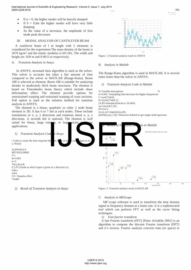
A. Transient Analysis in Ansys

In ANSYS, newmark beta algorithm is used as the solver. This solver is accurate but takes a fair amount of time compared to the solver in MATLAB (Runge-Kutta). Beam 188 is selected as element. Beam 188 is suitable for analyzing slender to moderately thick beam structures. The element is based on Timoshenko beam theory which include shear deformation effect. The element provide options for unrestrained warping and restrained warping of cross sections. Full option is used as the solution method for transient analysis in ANSYS.

The element is a linear, quadratic or cubic 2 node beam element in 3D. It has 6 or 7 dof at each nodes. These include translations in x, y, z directions and rotations about x, y, zdirections. A seventh dof is optional. The element is well suited for linear, large rotation, or large strain nonlinear applications.

1) Transient Analysis Code in Ansys

! Code to create the time response between input at node x and output at node y, Hxy(t)

ALPHAD,0.9 BETAD,0.00001 f=1 dt=0.001 ts=2 *do,t,dt,ts,dt F,2,FY,f!node at which input is given in y direction (x) time,t solve f=0 !Impulse effect *enddo

2) Result of Transient Analysis in Ansys

1

-.6

-.4

-.2

0

.2

.4

.6

.8

1

1.2

1.4

(x10**-3)

VALU

0.1

.2.3

.4.5

.6.7

.8.9

1

TIME

AUG 19 201423:19:45

POST26

UY_2

Figure. 1.Transient analysis result in ANSYS

B. Analysis in Matlab

The Runge-Kutta algorithm is used in MATLAB. It is several times faster than the solver in ANSYS.

1) Transient Analysis Code in Matlab

% Variable descriptions % ts=0.001; %sampling time decrease for higher frequencies C=eye(2*sdof); D=zeros(2*sdof,1); [A,B]=statespace(mn,kn,cc,ff,sdof); sys=ss(A,B,C,D); t0=0:ts:5; [yy,tt,xx]=impulse(sys,t0); plotfft(tt,yy(:,12)); %function defined to get single sided spectrum

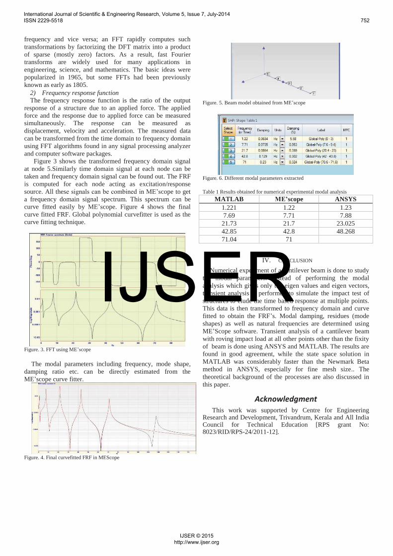
2) Result of Transient Analysis in Matlab

0 50 100 150 200 250 300

0

2

4

6

8

10

12

14

16

18

20

X: 1.221Y: 6.559

Single-Sided Amplitude Spectrum of yy(t)

Frequency (Hz)

|Y(f)

|

X: 7.69Y: 18.62

X: 21.73Y: 11.1

X: 42.85Y: 4.87

X: 71.04Y: 5.732

X: 172.6Y: 1.016X: 118

Y: 0.5478

Figure. 2. Transient analysis result in MATLAB

C. Analysis in MEScope ME’scope software is used to transform the time domain

signal to frequency domain at a faster rate. It is a sophisticated tool which can perform FFT as well as the curve fitting techniques.

1) Fast fourier transformA fast Fourier transform (FFT) [Peter Avitabile 2001] is an

algorithm to compute the discrete Fourier transform (DFT) and it’s inverse. Fourier analysis converts time (or space) to



IJSER

frequency and vice versa; an FFT rapidly computes such transformations by factorizing the DFT matrix into a product of sparse (mostly zero) factors. As a result, fast Fourier transforms are widely used for many applications in engineering, science, and mathematics. The basic ideas were popularized in 1965, but some FFTs had been previously known as early as 1805.

2) Frequency response functionThe frequency response function is the ratio of the output

response of a structure due to an applied force. The applied force and the response due to applied force can be measured simultaneously. The response can be measured as displacement, velocity and acceleration. The measured data can be transformed from the time domain to frequency domain using FFT algorithms found in any signal processing analyzer and computer software packages.

Figure 3 shows the transformed frequency domain signal at node 5.Similarly time domain signal at each node can be taken and frequency domain signal can be found out. The FRF is computed for each node acting as excitation/response source. All these signals can be combined in ME’scope to get a frequency domain signal spectrum. This spectrum can be curve fitted easily by ME’scope. Figure 4 shows the final curve fitted FRF. Global polynomial curvefitter is used as the curve fitting technique.

Figure. 3. FFT using ME’scope

The modal parameters including frequency, mode shape,damping ratio etc. can be directly estimated from the ME’scope curve fitter.

Figure. 4. Final curvefitted FRF in MEScope

Figure. 5. Beam model obtained from ME’scope

Figure. 6. Different modal parameters extracted

Table 1 Results obtained for numerical experimental modal analysis MATLAB ME’scope ANSYS

1.221 1.22 1.237.69 7.71 7.88

21.73 21.7 23.02542.85 42.8 48.26871.04 71

IV. CONCLUSION

Numerical experiment of a cantilever beam is done to study the modal parameters. Instead of performing the modal analysis which gives only the eigen values and eigen vectors, transient analysis is performed to simulate the impact test of structures to elude the time based response at multiple points. This data is then transformed to frequency domain and curve fitted to obtain the FRF’s. Modal damping, residues (mode shapes) as well as natural frequencies are determined using ME’Scope software. Transient analysis of a cantilever beam with roving impact load at all other points other than the fixity of beam is done using ANSYS and MATLAB. The results are found in good agreement, while the state space solution in MATLAB was considerably faster than the Newmark Beta method in ANSYS, especially for fine mesh size.. The theoretical background of the processes are also discussed in this paper.

Acknowledgment This work was supported by Centre for Engineering

Research and Development, Trivandrum, Kerala and All India Council for Technical Education [RPS grant No: 8023/RID/RPS-24/2011-12].



IJSER

References

[1] Michael R. Hatch (2001), Vibration Simulation Using MATLAB and ANSYS, Chapman & Hall/CRC, ISBN 1-58488-205-0

[2] Atkinson, Kendall A. (1989), An Introduction to Numerical Analysis (2nd ed.), New York: John Wiley & Sons, ISBN 978-0-471-50023-0.

[3] Newmark, N. M. (1959) A method of computation for structural dynamics. Journal of Engineering Mechanics, ASCE, 85 (EM3) 67-94.

[4] Ascher, Uri M.; Petzold, Linda R. (1998), Computer Methods for Ordinary Differential Equations and Differential-Algebraic Equations, Philadelphia: Society for Industrial and Applied Mathematics, ISBN 978-0-89871-412-8.

[5] Ilker Tanyer (2008) Parameter Estimation for Linear Dynamical Systems With Applications to Experimental Modal Analysis. Master of Science Thesis, Izmir Institute of Technology

[6] Brigham, E. O. (2002). The Fast Fourier Transform. New York: Prentice-Hall

[7] Peter Avitabile,(2001) “Experimental Modal Analysis - A Simple Non Mathematical Presentation” Sound And Vibration

[8] Caughey, T.K., O’ Kelly, M.E.J. “Classical Normal Modes in Damped Linear Dynamic Systems” Transactions of ASME, Journal of Applied Mechanics 32 (1965) 583-588.



IJSER

numerical experiment to study the modal characteristics … · impulse response in matlab. ......

Documents