object-oriented software tools for the construction of...

Object-Oriented Software Tools for the Construction of Preconditioners *

EVA MOSSBERG, KURT OTTO, AND MICHAEL THUNE

Department of Scientific Computing, Uppsala University, Box 120, SE-751 04 Uppsala, Sweden; e-mail: { evam, kurt, michael}@ tdb. uu. se

ABSTRACT

In recent years, there has been considerable progress concerning preconditioned iterative methods for large and sparse systems of equations arising from the discretization of differential equations. Such methods are particularly attractive in the context of high-performance (parallel) computers. However, the implementation of a preconditioner is a nontrivial task. The focus of the present contribution is on a set of object-oriented software tools that support the construction of a family of preconditioners based on fast transforms. By combining objects of different classes, it is possible to conveniently construct any preconditioner within this family.

The implementation is made in Fortran 90, and uses the language features for abstract data types. Numerical experiments show that the execution time of programs based on the new tools is comparable to that of corresponding programs where the preconditioner is hardcoded. Moreover, it is demonstrated that both the initial preconditioner construction and subsequent modifications are easily done with our software tools, whereas the same tasks are very cumbersome for a hardcoded program.

The new tools are integrated into Cog ito, which is a library of object-oriented software tools for finite difference methods on composite grids.

1 INTRODUCTION This work deals with the extension of the Cogito tools to implicit methods.

For many significant applications in science and engineering, for instance in fluid dynamics or electromagnetics, the mathematical models consist of time-dependent partial differential equations (PDEs). Finite difference methods is one of the important classes of numerical methods for such problems. In the Composite Grid Software Tools (Cogito) project [35, 36], Rantakokko and Olsson have implemented object-oriented software tools for explicit finite difference methods on composite grids.

*This research was supported by the Swedish Research Council for Engineering Sciences.

© 1997 lOS Press ISSN 1058-9244/97/$8 Scientific Programming, Vol. 6, pp. 285-295 (1997)

When using an implicit method we obtain a system of linear equations. The coefficient matrix is large, sparse, and highly structured, but for hyperbolic problems often nonsymmetric and not diagonally dominant. Otto and Holmgren [ 11, 13, 14, 26] have developed frameworks for the construction of preconditioners based on fast transforms suitable for solving this type oflinear systems with iterative methods.

The new software tools are designed to support the discretization of the problem and the construction of the preconditioner. This is done with an object-oriented approach, where data types and operations are encapsulated in classes to achieve flexible and reusable programs. The tools are implemented in Fortran 90. The classes also

286 MOSSBERG, OTIO, AND THUNE

contain implementations of operations typically used in Krylov subspace methods [4].

We begin our discussion with an overview of related projects in Section 2. In Section 3, we show how Cogito can be extended to handle implicit methods, and in Section 4 we give a model problem and briefly describe the principles for the preconditioners we have used. The new classes are presented in Section 5, followed by case studies including numerical results in Section 6.

2 RELATED WORK

In the past, several research groups have made efforts at designing programming tools, environments, and languages for high-performance scientific computing. In many of these projects, there was too much emphasis on finding a suitable, expressive notation, and too little attention paid to efficiency and applicability to realistic problems (e.g., [29, 31]). In our project, we aim at avoiding this pitfall.

Other projects studied efficiency aspects in detail, notably the research that led to the development of High Performance Fortran (HPF) (e.g., [19, 33]). However, HPF as such does not lead to an improved software structure. HPF might be a language for the implementation of the tools we are considering.

The essential idea of our efforts on mathematical software tools is to apply modern software techniques (object-oriented analysis and design- OOAD) in order to develop a set of software tools that are flexible, and lead to portable programs that are easy to construct and modify. In recent years, there has been a rapidly growing interest in applying object-oriented ideas to the field of numerical software. Most of these efforts consist in enriching the programming language (normally C++) with some abstract data types (ADTs) suitable for scientific computing. Typical examples are arrays, matrices, grids, and stencils [16, 21, 38]. The overall style of programming remains procedure-oriented. There is a main program and procedures implementing the mathematical problem to be solved and the numerical method.

This is a big leap forwards compared with the traditional programming style in scientific computing. The new ADTs hide low-level implementation details, and thus make the programs easier to modify and to port. However, with the type of approach discussed above, it is still difficult to change to a new numerical method, or to change the mathematical problem to solve with a given method. In order to achieve this kind of flexibility, it is necessary with a fully object-oriented approach, such that the complete algorithm can be composed of different objects in a "plug-and-play" manner. Our ambitions go in this direction.

Other efforts similar to ours in spirit are Diffpack [3] and ELEMD [23]. In contrast to ours, these projects emphasize finite element methods. PETSc [1] is another interesting project with a similar approach, focusing, so far, mainly on linear algebra problems, but having in mind linear systems arising from the discretization of PDE problems.

The POOMA framework [28] addresses the same general issues as our project, and with a similar approach, but with differences in details. Especially, our top level of abstraction, Cogito/Solver, has no apparent counterpart in POOMA.

Let us finally mention that we have a cooperation with the Overture [2] and ObjectMath [5] projects. The C++ library Overture is similar in scope to our Fortran 90 library Cogito/Grid (see below). However, we focus more on the object-oriented analysis, aiming at the "plug-and-play" concept discussed above. ObjectMath is a software environment for object-oriented specification of mathematical models. A pilot project [15] has shown that ObjectMath and Cogito may be combined into a user-friendly problem solving environment. This line of research will be continued.

The list of related work could be made even longer, including also approaches that are not object-oriented. Suffice it here to note that the general issue of raising the level of abstraction in software for scientific computing is currently being addressed by a large number of research groups around the world. Many of these efforts are so successful that it is appropriate to say that we are currently seeing a breakthrough in the area of numerical software.

3 IMPLICIT METHODS IN COGITO

The numerical solution of PDEs includes a large number of choices. If we solve a given time-dependent PDE problem with a finite difference method, we must make decisions on issues such as domain discretization, space derivative approximations, and time-marching scheme. To develop new solution methods we may want to experiment with different boundary conditions, or different types of discretization stencils on different parts of the domain. With object-oriented techniques, we can implement PDE solvers as collections of components such as the ones described above. This approach yields flexible and extendible software tools, useful both in the development of numerical methods and for applications.

3.1 The Cogito Project

Cogito is an object-based class library for time-dependent PDEs on structured, possibly composite, grids [35]. The object-oriented approach used in Cogito is suitable when

developing a code easy to reuse and extend [30, 34]. An object-oriented design, however, is not the same as an implementation in an object-oriented language. For highperformance computing, Fortran 77 and Fortran 90, with the ability to call optimized library routines, has a strong position. The lower [25] and middle [27]level classes in Cogito are implemented in Fortran 77 and Fortran 90, and a top layer in C++. This top layer, Cogito/Solver [39], has a high level of abstraction, and utilizes the inheritance features of C++ to handle complex objects such as an entire PDE problem. So far, tools for explicit time-marching methods are supplied in the software library.

3.2 Implicit Solution Methods

When solving PDE problems with finite differences, the time step for an explicit method may be prohibitively small, limited by the stability criterion. An example of such an application is almost incompressible flow [6, 7, 12] where there are different time scales in the problem. An alternative way to solve the problem would then be to use an implicit time-marching method. This results in a system of linear equations

Bu = g (3.1)

to be solved for each time level. The discretization of time-harmonic and time-independent PDEs also leads to systems of equations. The matrix B is very sparse and highly structured, which indicates that an iterative method should be used to solve the system. To attain an acceptable rate of convergence, we do not solve (3.1 ), but rather the (left) preconditioned system

(3.2)

The focus of this work is the introduction of Fortran 90 classes that, in cooperation with the Grid and GridFunction classes in Cogito/Grid [27], can be used as building blocks in an implicit preconditioned PDE solver.

Note that we do not reinterpret system (3 .1) as a linear algebra problem. The entire solution process is expressed in terms of GridFunctions and operations on those. In related projects, such as PETSc [1], (3.1) would have to be formulated in matrix-vector notation before the iterative solver could be applied. Our approach is more convenient when the system is a discretization of a PDE. (On the other hand, the PETSc tools are applicable also to systems not originating from PDEs.)

3.3 Design

The elements of the coefficient matrix B in Equation (3 .1) depend both on the original mathematical.PDE problem

SOFfWARE TOOLS FOR PRECONDITIONERS 287

System

? - - - - j - l \

Grid f--. Grid r-1- Operator Function I

- - - - - - -.-/ ? l J L

Coefficient Stencil Boundary Condition

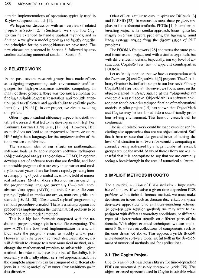
FIGURE 1 OMT diagram [30] with classes to identify and form the system of equations.

Pre- - Grid conditioner Function

y l I

Transform Operator

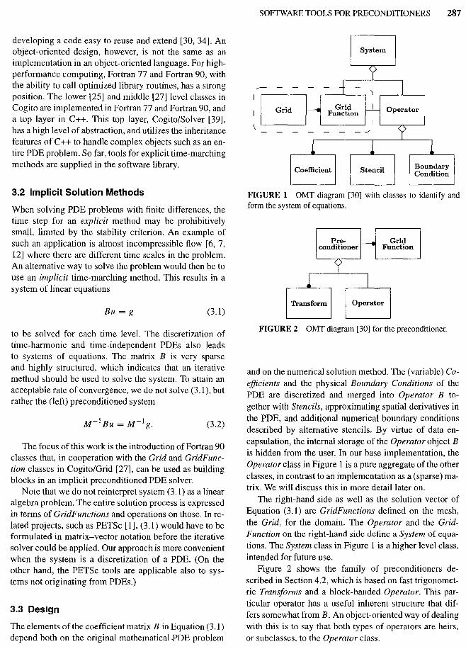
FIGURE 2 OMT diagram [30] for the preconditioner.

and on the numerical solution method. The (variable) Coefficients and the physical Boundary Conditions of the PDE are discretized and merged into Operator B together with Stencils, approximating spatial derivatives in the PDE, and additional numerical boundary conditions described by alternative stencils. By virtue of data encapsulation, the internal storage of the Operator object B is hidden from the user. In our base implementation, the Operator class in Figure 1 is a pure aggregate of the other classes, in contrast to an implementation as a (sparse) matrix. We will discuss this in more detail later on.

The right-hand side as well as the solution vector of Equation (3.1) are GridFunctions defined on the mesh, the Grid, for the domain. The Operator and the GridFunction on the right-hand side define a System of equations. The System class in Figure 1 is a higher level class, intended for future use.

Figure 2 shows the family of preconditioners described in Section 4.2, which is based on fast trigonometric Transforms and a block-banded Operator. This particular operator has a useful inherent structure that differs somewhat from B. An object-oriented way of dealing with this is to say that both types of operators are heirs, or subclasses, to the Operator class.


4 DISCRETIZATION AND PRECONDITIONING

Having in mind the Euler and Navier-Stokes equations describing gas or fluid flows, we now introduce a twodimensional model equation and discuss numerical methods for the discretized problem. The model problem is linear, but for a real-world problem the same type of systems of linear equations can appear in the solution procedure.

4.1 Model Problem

Consider the two-dimensional problem

with boundary and initial conditions. Here, the solution vector u is of size nc. The coefficients Ac = Ae(x, y), Be = Bc(x, y), and C = C(x, y) are nc x nc matrices and the source term g = g(x, y, t) is an nc-vector. We solve this second-order PDE using finite difference approximations on a logically rectangular grid.

As mentioned in the previous section, an efficient way to handle this problem may require an implicit method. If the spatial discretization is done on an mx x my grid, the sparse system (3 .1) is of size N = ncm x my.

4.2 Preconditioners

Any solver for the resulting systems of equations fits into the object-oriented design shown in Figure 1. Furthermore, in the context of preconditioned iterative solvers, any type of preconditioner can be used. However, the present contribution has a particular focus on a family of preconditioners, developed by Otto and Holmgren, expressed in Figure 2. For the problem ( 4.1) reduced to the scalar (nc = 1) case in one space dimension, i.e.,

au au a2u -+A-+B-+Cu=g, at ax ax2

a preconditioner of this family is a linear combination of normal matrices Rr:

M = LYrRr (4.2)

with scalar coefficients Yr. When solving the two-dimensional problem (4.1), the

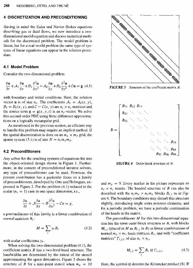
coefficient matrix B has a two-level band structure. The bandwidths are determined by the extent of the stencil approximating the space derivatives. Figure 3 shows the structure of B for a nine-point stencil when mx = 10

FIGURE 3 Structure of the coefficient matrix B.

B=

FIGURE 4 Outer block structure of B.

and my = 9. Every marker in the picture represents an nc x nc matrix. The banded structure of B can also be described with the ncmx x ncmx blocks Bi,.i as in Figure 4. The boundary conditions may disturb this structure slightly, introducing single extra nonzero elements, and for a periodic problem, we have a periodic continuation

of the bands in the matrix. The preconditioner M for this two-dimensional equa

tion has the same outer block structure as B, with blocks

Mi,.i (placed in M as Bi,.i in B) as linear combinations of normal mx x mx basis matrices Rr. and with "coefficient

matrices" ri,j,r Of size nc X nc,

(4.3)

Here, the symbol® denotes the Kronecker product [8]. If

ai; are elements of an m x n matrix A, then

The approximations studied are either optimal, minimizing liB - Mll.r to obtain y, or ri,J,r• or blockwise superoptimal, minimizing Ill- M7 .Bi,;ll.r, where M 7

. l,J . l,J is the pseudoinverse of Mu. The Frobenius matrix norm II · ll.r is given by

m n

IIAII.r= LL1aii1 2.

i=1}=1

For superoptimal approximations, the expressions in ( 4.2) and ( 4.3) are used for M 7 and Mt;. Different choices of the basis matrices R, correspond to different fast trigonometric transforms. These possibilities and the computation of the coefficients were first described in [13], and later generalized in [26].

If an iterative Krylov subspace method is applied to (3.2), an approximate solution u may be obtained faster when the preconditioner M is formed not from B, but from a modified matrix B. This matrix represents the discretization of ( 4.1 ), using the same interior stencil as for B, but with altered boundary conditions.

In [ 14] it is shown that the preconditioner solve u = M- 1 g for these preconditioners can be performed using the following three-step algorithm:

1. Perform ncmy independent fast transforms of length mx.

2. Solve mx independent systems of ncmy equations, which are block banded with ( *) block size nc x nc.

3. Perform ncmy indepedent fast inverse transforms of length m x.

Note the independence in each of the three steps, which makes the procedure well suited for efficient parallel implementations [10]. This algorithm is the reason for the object model in Figure 2. As pointed out before, the model is specific to this family of preconditioners, but the classes in Section 5 are useful together with a wide range of preconditioners.

5 CLASSES

We use the word class to describe our Fortran 90 units. Classes consist of abstract data types and operations on


those, encapsulated in modules, protected from the surrounding classes with private declarations. Norton, Szymanski, and Decyk [24] did a study on the object-oriented features of C++ and the Fortran 90 features for abstract data types, in high-performance computation, and found them comparable. The performance of their Fortran 90 code, using the same kind of encapsulation techniques as Cogito, was far better than their C++ version, although worse than a traditional well-tuned Fortran 77 implementation for the problem. Another comparison of languages in computational science is done in [37] with respect to numerical robustness, data parallelism, data abstraction, and object-oriented programming, and this places Fortran 90 ahead of both C++ and Fortran 77.

In Subsections 5.1-5.7 we describe the classes depicted in Figures 1 and 2. The interfaces for the classes are done in the object-oriented manner with constructors, destructor, selectors (information routines, giving access to values and parameters stored by the class), and modifiers (subroutines to change the object's datafields). A more detailed description of each and every one of the new classes can be found in [22].

5.1 GridFunction

A GridFunction represents the numerical solution of the PDE or the right-hand side of a system of equations. Each gridfunction is defined on a (possibly composite) mesh, an object of the class Grid, and has information of subdomains defined on the mesh. Typically, such subdomains model the boundaries. The Grid and GridFunction classes are described in detail in [27] and [36]. We have added operations to apply an operator to a gridfunction, produce the inner product of two gridfunctions, and to do the preconditioning. As an example of the style of the code, the preconditioning operations are listed below:

ApplylnvPrecond(gf, M, x)

Preconditioner solve gf = M- 1 x. This is done with the aid of operations FastTransf, FastlnvTransf, and SolveBandSystem, corresponding to the three-step algorithm ( * ).

FastTransf(gf, Q(l:L, 1:1), x)

The gridfunction gf is the result of applying the fast transforms Q(f, j), in the coordinates f = 1, ... , L for the components j = 1, ... , 1, to the gridfunction x.

FastlnvTransf(gf, Q(l:L, 1:1), x)

The gridfunction gf is the result of applying the inverses of the fast transforms to the gridfunction x.

SolveBandSystem(gf, N, x)

Solve the banded system N gf = x, where gf and x are gridfunctions.

290 MOSSBERG, OTTO, AND THUNE

5.2 Coefficient

The class Coefficient represents the discretized coefficients in Equation ( 4.1 ). The input is a function that contains the formula for the coefficients. In the present implementation, for space-dependent coefficients only, the function is evaluated once on the entire grid, and the values are stored. To allow for coefficients with space and

time dependency, repeated function calls would be an alternative.

5.3 Stencil

Every term (the identity operation or a derivative of first or higher order) in Equation ( 4.1) is approximated by a finite difference- a stencil. An object of the class Stencil is a one-dimensional set of offsets, described by the space direction (x or y) of the stencil, its extension from the central point, and the weights associated with each offset. In the present implementation, "empty" offsets within the range must be assigned zero weights. To apply the complete operator to a gridfunction, we apply the different stencils on the corresponding subdomains.

5.4 BoundaryCondition

An object of the BoundaryCondition class has information on what type of local boundary condition it handles, in which space direction this condition is applied, and if the PDE problem has a nonhomogeneous boundary condition of Dirichlet or Neumann type, the boundary data are stored. The present implementation also supports periodic boundary conditions.

5.5 Operator

The class Operator represents the total operator B of the discretized problem (3.1). In this implementation, it is not at all stored as a matrix, but as a set of objects of other classes. Most importantly, there are stencils with information about which subdomain of the grid each stencil should be applied to. See also the GridFunction class.

5.6 Transform

So far, the preconditioners described in Subsection 4.2 make use of the Fourier transform, sine transform, cosine transform, or some modification of one of them. The design will make it easy to use this new set of Cogito tools to develop and test new preconditioners within this family.

5.7 Preconditioner

This is an implementation of the preconditioners based on fast transforms described above. However, the interfaces provided by the operations, e.g., to do the (nontrivial) setup of the preconditioner, should be suitable for many types of preconditioners. This is where the theoretical framework, developed in [13], is exploited. The framework allows different approximation types (optimal or superoptimal), and different types of fast trigonometric transforms.

In order to form the preconditioner, we need to access the values corresponding to the weights of the total space discretization stencil for every grid line. We have not stored the total stencil in our Operator objects. When the operator is applied to a gridfunction, each and every one of the derivative Stencils is applied separately. Thus, we have to apply the operator to gridfunctions that are concatenations of smaller "unit" gridfunctions to extract the desired values. In a typical PDE solving program, this not so straightforward procedure is done only once, whereas matrix-vector multiplications (applying an operator to a gridfunction) are repeated over and over again. That is why we have chosen an implementation that favors the latter.

6 CASE STUDIES

In this section, we describe a PDE problem and show how the implementation can be done, and easily modified, using the described tools. We also show by example how expressive the new gridfunction operations are.

6.1 Wave Equation

Consider the two-dimensional wave equation with Dirichlet boundary conditions:

au au au 1 - +-+- = (2- v)f (XI+ X2- Ut) (6.1) at axl axz

for 0<x1~a1, O<x2~a2, t>O,

where

u(O, x2, t) = j(x2- vt),

u(XJ, 0, t) = f(xi- vt),

u(xi,Xz,O) = f(xl +x2),

f(y) = sin(7y),

and 0 < v « 1 is a velocity parameter introduced to model a slow time scale.

To model a stretched grid, where the gridpoints lie more densely near the boundaries, we introduce the coordinate transformations

xe = ae ( tanh(se (2~e - 1)) + ~), 2 tanh(se) 2

0 < ~e :S: I, f = I, 2. (6.2)

The positive parameters s1 and s2 control the stretching of the grid. Larger se gives a mesh that is more stretched in direction£. In fact, as se -+ 0, the transformation (6.2) becomes just a scaling by ae.

Using this, Equation (6.1) transforms into a PDE with variable coefficients

au au au - + O"j(~I)- + 0"2(~2)at a~1 ab

=(2-v)J'(x!+X2-vt), (6.3)

where

1 2 tanh(se) O"£(~e)=a( cosh (se(2~e-1)) .

Sf (6.4)

We then solve (6.3) on a uniform grid. The computational domain 0 < ~e ::;; I, f = I, 2, is

discretized with space step he in direction £. In the interior we approximate the spatial derivatives in (6.3) with the second-order accurate stencil Do, and at the outflow boundary~£ = I with first-order accurate D_. Figure 5 shows the stencils approximating au 1 a~. u we define P as the total space discretization operator, and use the trapezoidal rule for implicit time discretization of (6.3), the scheme can be written as

Here un is the solution vector, i.e., the gridfunction at time level n, and k is the time step. The system of equations to solve for time level n + 1 becomes

1 2h

Do

(I+ ~kP) un+l = rn. '-.,-'

B

1 2h

D_

FIGURE 5 Space discretization stencils.

1 h


6.2 Implementation

In the Fortran 90 implementation, we must begin with a number of declarations and allocations. The syntax for this is a bit more complicated than for an analogous library in C++, but the solver subroutine below can be written in a fairly transparent way.

program

! Declarations

external bcFunc external transFunc

! Create a grid. Coordinates are read from file. call Create_G(g, 'grid.dat') call Read_G (g) gsz = Size_G(g)

! Define subdomains, ! corresponding to boundary areas. east(1) = gsz(1); east(2) = gsz(1); east(3) = 1; east(4) = gsz(2) id = 101 call DefSD_G(g,east,id) north(1) id = 102

! Create and initiate two gridfunctions ! on the grid, one with initial values, ! and one with the right-hand side of ! the system of linear equations. call Create_GF(xO,nc,g) call Create_GF(rhs,nc,g)

! Dirichlet condition in the x 1-direction.

direc = 1 call Create_BoundCond(bcD, &

direc, 'D' ,gsz,bcFunc)

! Here, transFunc refers to ! Equation (6.4) for f = 1. call Create_Coeff(sigma1, &

nc,gsz,transFunc)

! Make a stencil by defining its weights. w(-1) = -0.5; w(O) = 0.0; w(1) = 0.5 w = w/h1 call Create_Stencil(Dzerox,direc,w)

! Initiate the construction of the operator, ! and add the coefficients and stencils to it. ! The optional parameters alpha and beta


! determine the time discretization. alpha= 1.0; beta= 0.5 call Create_Operator(B, &

bcD,gsz,nc,alpha,beta) call Build_Operator(B, &

sigmal,Dzerox,id)

! Here we use the Fourier transform. call Create_Transform(Q(l:l,l:l), &

'FT')

! Form the preconditioner, ! '0' for optimal approximation, ! or ' S ' for superoptimal. call Create_Precond(M,B,Q, '0')

! Solve the resulting system!

! Explicit destructor call call Delete_G(g)

end program

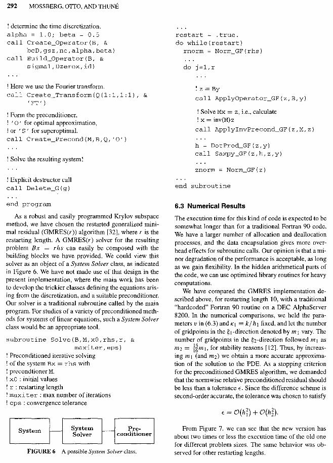
As a robust and easily programmed Krylov subspace method, we have chosen the restarted generalized minimal residual (GMRES(r)) algorithm [32], where r is the restarting length. A GMRES(r) solver for the resulting problem Bx = rhs can easily be composed with the building blocks we have provided. We could view this solver as an object of a System Solver class, as indicated in Figure 6. We have not made use of that design in the present implementation, where the main work has been to develop the trickier classes defining the equations arising from the discretization, and a suitable preconditioner. Our solver is a traditional subroutine called by the main program. For studies of a variety of preconditioned methods for systems of linear equations, such a System Solver class would be an appropriate tool.

subroutine Solve(B,M,xO,rhs,r, & maxiter,eps)

! Preconditioned iterative solving ! of the system Bx = rhs with ! precondtioner M. ! xO : initial values ! r : restarting length ! maxi ter : max number of iterations ! eps : convergence tolerance

System Pre-System f-- Solver r--- conditioner

FIGURE 6 A possible System Solver class.

restart = .true. do while(restart)

rnorm = Norm_GF(rhs)

do j=l,r

! z =By

call ApplyOperator_GF(z,B,y)

! Solve Mx = z, i.e., calculate ! x = inv(M)z

call ApplyinvPrecond_GF(z,M,z)

h = DotProd_GF(z,y) call Saxpy_GF(z,h,z,y)

znorm = Norm_GF(z)

end subroutine

6.3 Numerical Results

The execution time for this kind of code is expected to be somewhat longer than for a traditional Fortran 90 code. We have a larger number of allocation and deallocation processes, and the data encapsulation gives more overhead effects for subroutine calls. Our opinion is that aminor degradation of the performance is acceptable, as long as we gain flexibility. In the hidden arithmetical parts of the code, we can use optimized library routines for heavy computations.

We have compared the GMRES implementation described above, for restarting length 10, with a traditional "hardcoded" Fortran 90 routine on a DEC AlphaServer 8200. In the numerical comparisons, we held the parameters v in (6.3) and KJ = k/ h 1 fixed, and let the number of gridpoints in the ~ 1-direction denoted by m 1 vary. The number of gridpoints in the ~z-direction followed m 1 as m2 = ~m 1 , for stability reasons [12]. Thus, by increasing m 1 (and mz) we obtain a more accurate approximation of the solution to the PDE. As a stopping criterion for the preconditioned GMRES algorithm, we demanded that the norm wise relative preconditioned residual should be less than a tolerance E. Since the difference scheme is second-order accurate, the tolerance was chosen to satisfy

From Figure 7, we can see that the new version has about two times or less the execution time of the old one for different problem sizes. The same behavior was observed for other restarting lengths.

2.5 s :0 2 ;:l 0.

~1.5 Qi ...

: ,_1 ::::i 100 : .. ···············

v = 0.06"

5.5 6 6.5 7 7.5 8 8.5 9 9.5 10 log2 (mi)

• ,.1 ::::; 1000 ........ , ........ · ........ · ........ . . ..................... : .. ..... : .......... : .. .

v == 0.01:

6 6.5 7 7.5 8 8.5 9 9.5 10 log2 (mi)

FIGURE 7 Relative performance for the GMRES(IO) solver for two different values of KJ and v.

Moreover, it can be noted that the relative performance of the Cogito-based solver is better for larger problem sizes. This is expected, as the overhead costs should remain constant, whereas the computation time increases independently of approach. We consider this loss in performance to be a fair price. For sufficiently large problem sizes, the effect of internal calls will be negligible. With the new software tools, we have an excellent starting point for experiments with, e.g., stencils or boundary condition changes. One of our primary goals is to use the new setup for development of new preconditioners.

6.4 Modification of the Scheme

In the traditional code we had poor support for modifications of the numerical scheme. The following example illustrates this, and shows that the new software tools improve the situation dramatically. In order to damp highfrequency oscillations in our wave propagation problem, we may modify the operator by adding artificial dissipative terms

for the interior gridpoints in both directions. This change is mirrored in the coefficient matrix, possibly adding bandwidth to it, as well as changing already nonzero elements. For the traditional code, it would be a tedious and time-consuming problem to rewrite the assembly of the matrix. This is particularly noticeable in the context of adaptivity, where such as modification would be done


only on a more limited part of the computational domain. However, making the same modification, using our new software tools, is an uncomplicated task. We just add a few lines to our main program:

! Create the additional stencil and coefficient.

w(-1) = -1.0; w(O) = 2.0 w(1) = -1.0; w = w/(h1**2) call Create_Stencil(DplusDminus, &

direc,w) call Create_Coeff(epsh,nc,gsz,func)

! The id parameter here denotes ! interior points in the x 1-direction.

call Build_Operator(B, & epsh,DplusDminus,id)

6.5 Expressiveness

The purpose of this subsection is to demonstrate how useful and expressive the operations defined in Subsection 5.1 actually are. To this end, we consider the normal block preconditioners in [26] referred to as being polytransform with several block levels. Such preconditioners are aimed at discretized systems of PDEs, where the components of the solution depend on L coordinates. The basic idea for a polytransform preconditioner with several block levels is to apply fast transforms in all coordinates but one, and to allow different transforms for different coordinates and components. For the remaining coordinate, block banded systems are solved, and the preconditioning is completed by inverse transforms. If the discretized solution is embedded in a vector, the transform part of the preconditioner could be expressed as a matrix with a hierarchy of L block levels. However, that matrix is muddled with permutation matrices [26], which are needed in order to get the various transforms applied correctly. The structure of the preconditioning operator becomes much clearer when the operand is represented as a tensor of order L + 1, i.e., one index for each of the L discretized coordinates and one component index. Note that the Cogito concept of a gridfunction is closely related to such a tensor. In fact, gridfunctions in Cogito are actually implemented as arrays of dimension L + 1.

In the preconditioning algorithm below, the number of components is mo, and me denotes the number of discrete coordinate points for the coordinate labeled l = 1, ... , L. Thus, the total number of coordinate points is

The algorithm for a polytransform preconditioner with L block levels becomes:


1. Fore = 1, ... , L - 1 and Jo = 1, ... , mo, perform n LIme independent fast transforms of length me.

2. Solve nL-i independent systems of mLmo equations, which are block banded with block size mo x mo.

3. For£= 1, ... ,L-1and}o= 1, ... ,mo, perform nL/me independent fast inverse transforms of length me.

The algorithm (*)is just the special case where L = 2, mo = nc, m1 = mx, and m2 =my. By representing the solution and the right-hand side as gridfunctions z, the algorithm above is readily expressed in terms of operations from Subsection 5.1 as

1. Apply FastTransf(z, Q(L - 1:1, 1 :mo), z). 2. Apply SolveBandSystem(z, N, z). 3. Apply FastlnvTransf(z, Q(l :L - 1, 1 :mo), z).

Furthermore, it is now easy to build new preconditioners. By replacing the index range L - 1:1 with L: 1, we obtain a preconditioner where the operator N is block diagonal, which would be a clear advantage for the implementation on parallel computers. On the other hand, such a complete block diagonalization could, depending on the original operator B, degrade the convergence rate of the preconditioned Krylov subspace method. In that case, an alternative is to transform only in the coordinates that are amenable to fast transforms; typically those coordinates for which the coefficients of the operator B vary moderately. This is achieved by replacing the index range L - 1: 1 with an index set that selects the desired coordinates. However, by transforming in fewer coordinates than L - 1, the operator N will no longer be narrow banded. For each coordinate labeled e ~ L - 1 that is not transformed, the bandwidth of N is increased notably.

7 CONCLUDING REMARKS

We have presented ideas for an extension of Cogito to implicit methods, so that we get a flexible system for both explicit and implicit finite difference methods on structured grids. This extension does not limit the choice of discretization stencils. We expect that this freedom will be valuable for the development of new numerical methods.

Linked to this environment, we now also have techniques for effectively solving the systems of linear equations arising from the implicit methods. These solvers are preconditioned iterative methods, where the preconditioners are constructed from a general framework for fast transforms. The numerical performance of a GMRES solver built with the new tools is within a factor two of

that of a traditional code for sufficiently large problems. We find this cost acceptable for the achieved increase in flexibility.

We have now taken a first step to incorporate the handling of implicit methods in Cogito. A second step on the way to a complete parallel framework is to combine this work with a newly implemented parallel version of the Fortran 90 classes Grid and GridFunction. Being based on these, a large part of our classes will automatically execute in parallel. Further development is also necessary for the handling of composite grids and threedimensional grids in the new part of the code. Future directions of research could entail extensions to accommodate nonlocal boundary conditions such as Dirichlet-toNeumann maps [ 17], staggered grids, Schur complement matrix methods [9, 18, 20], and nonlinear PDEs.

ACKNOWLEDGEMENTS

We thank Peter Olsson, Jarmo Rantakokko, and Krister Ahlander in the Cogito group for explaining their ideas and codes. We are also grateful to Dr. Sverker Holmgren for supplying parts of the codes for the preconditioned Krylov subspace methods.

REFERENCES

[1] S. Balay, W. D. Gropp, L. Curfman Mcinnes, and B. F. Smith, "PETSc 2.0 users manual," Argonne Nat!. Lab., Argonne, IL, Rep. ANL-95/11, 1995.

[2] D. L. Brown and W. D. Henshaw, "Overture: An advanced object-oriented software system for moving overlapping grid computations," Los Alamos Nat!. Lab., Los Alamos, NM, Rep. LA-UR-96-2931, 1996.

[3] A. M. Bruaset and H. P. Langtangen, "Object-oriented design of preconditioned iterative methods in Diffpack," ACM Trans. Math. Software, vol. 23, pp. 50-80, 1997.

[4] R. W. Freund, G. H. Golub, and N. M. Nachtigal, "Iter

ative solution of linear systems," Acta Numerica, vol. 1,

pp. 57-100, 1992.

[5] P. Fritzson, L. Viklund, J. Herber, and D. Fritzson, "Indus

trial application of object-oriented mathematical modeling

and computer algebra in mechanical analysis," in Technol

ogy of Object-Oriented Languages and Systems- TOOLS

7, pp. 167-181, 1992.

[6] J. Guerra and B. Gustafsson, "A semi-implicit method for

hyperbolic problems with different time-scales," SIAM J.

Numer. Anal., vol. 23, pp. 734--749, 1986.

[7] B. Gustafsson and H. Stoor, "Navier-Stokes equations

for almost incompressible flow," SIAM J. Numer. Anal.,

vol. 28, pp. 1523-1547, 1991.

[8] P. R. Halmos, Finite-Dimensional Vector Spaces. New

York: Springer-Verlag, 2nd ed., 1974.

[9] L. Hemmingsson, "A domain decomposition method for first-order PDEs," SIAM 1. Matrix Anal. Appl., vol. 16, pp. 1241-1267, 1995.

[10] S. Holmgren, "CG-like iterative methods and semicirculant preconditioners on vector and parallel computers," Dept. of Scientific Computing, Uppsala Univ., Uppsala, Sweden, Rep. 148, 1992.

[11] S. Holmgren and K. Otto, "Iterative solution methods and preconditioners for block-tridiagonal systems of equations," SIAM 1. Matrix Anal. Appl., vol. 13, pp. 863-886, 1992.

[12] S. Holmgren and K. Otto, "Semicirculant solvers and boundary corrections for first-order partial differential equations," SIAM 1. Sci. Comput., vol. 17, pp. 613-630, 1996.

[13] S. Holmgren and K. Otto, "A framework for polynomial preconditioners based on fast transforms 1: Theory," BIT, Vol. 38, 1998 (to appear).

[14] S. Holmgren and K. Otto, "A framework for polynomial preconditioners based on fast transforms II: POE applications," BIT, Vol. 38, 1998 (to appear).

[15] P. Hagglund, P. Olsson, M. Thune, and P. Fritzson, "Imple

mentation of a POE application in ObjectMath and Cog

ito," Parallel and Scientific Computing Institute, Royal In

stitute of Technology, Stockholm, Sweden, Rep. 5, 1996.

[16] J. F. Karpovich, M. Judd, W. T. Strayer, and A. S.

Grimshaw, "A parallel object-oriented framework for sten

cil algorithms," in Proc. 2nd Int. Symp. High Performance

Distributed Computing, 1993, pp. 34-41.

[17] J. B. Keller and D. Givoli, "Exact non-reflecting boundary

conditions," 1. Comput. Phys., vol. 82, pp. 172-192, 1989.

[18] D. E. Keyes and W. D. Gropp, "A comparison of domain

decomposition techniques for elliptic partial differential

equations and their parallel implementation," SIAM 1. Sci.

Statist. Comput., vol. 8, pp. s166-s202, 1987.

[ 19] C. Koelbel and P. Mehrotra, "Compiling global name

space programs for distributed execution," I CASE, NASA

Langley Research Center, Hampton, VA, Rep. 90-70,

1990.

[20] E. Larsson, "A domain decomposition method for the

Helmholtz equation in a multilayer domain," Dept. of Sci

entific Computing, Uppsala Univ., Uppsala, Sweden, Rep.

190, 1996.

[21] M. Lemke and D. J. Quinlan, "P++, a parallel C++ ar

ray class library for architecture-independent development

of structured grid applications," ACM SIGPLAN Notices, vol. 28, no. 1, pp. 21-23, 1993.

[22] E. Mossberg, "Object-oriented software tools for the construction of preconditioners," Dept. of Materials Science, Uppsala Univ., Uppsala, Sweden, Rep. UPTEC 97 020E, 1997.

SOFTWARE TOOLS FOR PRECONDITIONERS 295

[23] G. Nelissen and P. F. Vankeirsbilck, "Electrochemical modelling and software genericity," in Modern Software Tools for Scientific Computing, E. Arge, A. M. Bruaset, and H. P. Langtangen, eds., Boston, MA: Birkhauser, 1997.

[24] C. D. Norton, B. K. Szymanski, and V. K. Decyk, "Objectoriented parallel computation for plasma simulation," Comm. ACM, vol. 38, no. 10, pp. 88-100, 1995.

[25] P. Olsson, "Object-oriented software tools for parallel computing with distributed memory," Dept. of Scientific Computing, Uppsala Univ., Uppsala, Sweden, Rep. 193, 1997.

[26] K. Otto, "A unifying framework for preconditioners based on fast transforms," Dept. of Scientific Computing, Uppsala Univ., Uppsala, Sweden, Rep. 187, 1996.

[27] J. Rantakokko, "Object-oriented software tools for composite-grid methods on parallel computers," Dept. of Scientific Computing, Uppsala Univ., Uppsala, Sweden, Rep. 165, 1995.

[28] J. V. W. Reynders et a!., POOMA: A framework for scientific computing applications on parallel computers. Los Alamos Nat!. Lab., Los Alamos, NM, http://www.acl.lanl.gov/PoomaFramework/.

[29] M. Rosing, R. B. Schnabel, and R. P. Weaver, "Dino: Summary and examples," in Proc. 3rd Conf Hypercube Concurrent Computers and Applications, 1988, pp. 472-481.

[30] J. Rumbaugh, M. Blaha, W. Premerlani, F. Eddy, and W. Lorensen, Object-Oriented Modeling and Design. Englewood Cliffs, NJ: Prentice-Hall, 1991.

[31] Th. Ruppelt and G. Wirtz, "Automatic transformation of high-level object-oriented specifications into parallel programs," Parallel Comput., vol. 10, pp. 15-28, 1989.

[32] Y. Saad and M. H. Schultz, "GMRES: A generalized minimal residual algorithm for solving nonsymmetric linear systems," SIAM 1. Sci. Statist. Comput., vol. 7, pp. 856-869, 1986.

[33] J. H. Saltz, R. Mirchandaney, and K. Crowley, "Runtime parallelization and scheduling of loops," !CASE, NASA Langley Research Center, Hampton, VA, Rep. 90-34, 1990.

[34] D. A. Taylor, Object-Oriented Technology: A Manager's Guide. Reading, MA: Addison-Wesley, 1993.

[35] M. Thune, "Object-oriented software tools for parallel POE solvers," Wuhan Univ. 1. Natur. Sci., vol. 1, pp. 420-429, 1996.

[36] M. Thune, P. Olsson, and J. Rantakokko, User's Guide, Cogito Documentation. Dept. of Scientific Computing, Uppsala Univ., Uppsala, Sweden, 1994-1995.

[37] J. L. Wagener, "Fortran 90 and computational science," in Computational Science Education Project, http://csep 1. phy.ornl.gov/csep.html, 1996.

[38] R. D. Williams, "DIME++: A language for parallel PDE solvers," Caltech, Pasadena, CA, Rep. CCSF-30, 1993.

[39] K. Ahlander, "An object-oriented approach to construct POE solvers," Dept. of Scientific Computing, Uppsala Univ., Uppsala, Sweden, Rep. 180, 1996.

Submit your manuscripts athttp://www.hindawi.com

Computer Games Technology

International Journal of

Hindawi Publishing Corporationhttp://www.hindawi.com Volume 2014


Distributed Sensor Networks


Advances in

FuzzySystems

Hindawi Publishing Corporationhttp://www.hindawi.com

Volume 2014


ReconfigurableComputing

Hindawi Publishing Corporation http://www.hindawi.com Volume 2014


Applied Computational Intelligence and Soft Computing

Advances in

Artificial Intelligence


Advances inSoftware EngineeringHindawi Publishing Corporationhttp://www.hindawi.com Volume 2014


Electrical and Computer Engineering

Journal of

Journal of

Computer Networks and Communications


Hindawi Publishing Corporation

http://www.hindawi.com Volume 2014

Advances in

Multimedia


Biomedical Imaging


ArtificialNeural Systems

Advances in


RoboticsJournal of



Computational Intelligence and Neuroscience

Industrial EngineeringJournal of


Modelling & Simulation in EngineeringHindawi Publishing Corporation http://www.hindawi.com Volume 2014

The Scientific World JournalHindawi Publishing Corporation http://www.hindawi.com Volume 2014


Human-ComputerInteraction

Advances in

Computer EngineeringAdvances in


object-oriented software tools for the construction of...

Documents