Obstacle Avoidance using Monocular Vision on

Micro Aerial Vehicles

J. M. SAGAR

10318771

Msc. THESIS

Credits: 42 ECTS

Master of Science in Artificial Intelligence

University of Amsterdam

Faculty of Science

Science Park 904

Supervisor: Arnoud Visser

Room C3.237

Science Park 904

NL 1098 XH Amsterdam

Abstract

For Micro Aerial Vehicles (MAVs), robust obstacle avoidance during flight is a challenging

problem due to limited payload they can carry. Due to limited battery capacity, only light

weight sensors such as monocular cameras can be mounted which don’t cause a toll on battery

life and weight limitations. The problem with monocular cameras for obstacle avoidance is

depth perception as vision disparity cannot be estimated with a single camera and stereo

cameras or additional sensors have to be used. We developed a method to focus only on regions

which were classified as foreground and follow features in the foreground to estimate threat of

potential objects being an obstacle in the flight path. For this we process video input from the

drone, classify foreground and background on a pixel level, filter results and track these pixels

using optical flow, assigning weights to determine closer pixels from further pixels. We

experiment and evaluate results from our approach in a series of obstacle courses with varying

levels of challenges using a small quad-rotor drone. We are able to determine evident obstacles

in front of the drone with high confidence for a variety of obstacles in various settings.

Acknowledgements

I would like to thank my supervisor Dr. Arnoud Visser for his guidance and influential

supervision throughout the study. I would also like to thank my parents Maheshbhai and

Heenaben for their constant support and faith throughout my master study. A special

appreciation to my sister Yesha and dear friend Sulaiman Azhar for their help with my

experiments and evaluation for this study.

I would like to give a special thanks to Ke Tran, George Visniuc, and Efstathios Charitos for

their help in understanding and following concepts that I required help with.

Table of Contents 1. Introduction ……………………………………………………………………………...1

2. Related Work ………………………………………………………………………..…...3

3. General Methods Used ……………………………………………….………………….7

3.1. Background/Foreground Classification ……………………………………………………7

3.2. Tracking and Depth Estimation …………………………………………..………………..10

3.2.1. Feature Detection …………………………………………………………….10

3.2.2. Tracking ……………………………………………………………………...12

3.2.3. Depth Classification ………………………………………………………….14

3.3. Template Matching ………………………………………………………………………….14

4. Proposed Method …………………………………………………..…………………...16

4.1. Background Subtraction …………………………………………………………………….17

4.2. Optical Flow ………………………………………………………………………...............20

4.3. Clustering……………………………………………………………………………………..21

4.4. Depth Segmentation ………………………………………………………………..............23

4.5. Proximity Estimation ………………………………………………………………………..24

5. Experiments and Discussion …………………………………………….……………..27

5.1. Tools ………………………………………………………………………………................27

5.1.1. Robot Operating System (ROS) ……………………………………………..27

5.1.2. OpenCV ……………………………………………………………………...27

5.1.3. Parrot A.R. Drone ……………………………………………………………28

5.1.3.1. Quad-Rotor Flight Control …………………………………………...29

5.1.3.2. Sensors ……………………………………………………………….30

5.1.3.3. On-Board Intelligence ………………………………………………..31

5.1.4. A.R. Drone Driver for ROS ………………………………………………….31

5.1.5. PC Configuration …………………………………………………………….32

5.2. General Experiments ………………………………………………………………………..32

5.2.1. Background/Foreground Classification ……………………………………...32

5.2.2. Feature Selection and Tracking ………………………………………………34

5.3. Flight Experiments ……………………………………………………….………………….37

5.3.1. Experiment 1: Single stationary narrow obstacle in an outdoor scene ………37

5.3.2. Experiment 2: Two stationary narrow obstacles in an outdoor scene ……….40

5.3.3. Experiment 3: Two wide obstacles in an outdoor scene ……………………..44

5.4. General Discussion ………………………………………………………………………….47

6. Conclusion …………………..…………………………………………………………..49

7. Future Work ……………………………………………………………………………50

8. References ……………………………………………………………………………….51

1

1 Introduction

Technological advances in terms of hardware and software allow for reproducing ideas from

science fiction stories to physical reality. In the domain of robot technology, we see a lot of

progress using sophisticated hardware and software coming together to create a functional

machine to accomplish varying tasks replicating human activity. From various domestic tasks

to complex intricate tasks, we see a positive future in research and development of such

machines. Today, MAVs (Micro Aerial Vehicles) are used for tasks such as surveys,

surveillance, search and rescue, and military applications which would otherwise be difficult

or infeasible for humans considering harsher and challenging conditions. However, this is a

challenging problem as activities that are simple and latent knowledge for living beings, are

non-trivial when replicating on machines. Technology in this domain still has a way to go to

achieve near human intelligence, but today, research tackles several sub-tasks which can

someday be integrate into a system.

Specific kinds of drones have been developed such as flappy-wing drones, fixed-wing drones,

and rotor based drones. Flappy wing drones have an advantage of being able to hover and fly

close to objects being small, agile, and less dangerous due to their low weight. Fixed-wing

drones are UAVs that use a gliding mechanism and use either external propulsion mechanism

or built in linear propellers. Unlike flappy wind drones, fixed-wing drones are not very agile

but have longer flight durations and are extensively used for surveying and mapping

applications. Rotor based drones have a number of rotors that keep the drone aloft and flight

control is based on regulating rotor speed giving it a wide degree of freedom in flight. Being

heavier and larger than flappy wing drones, rotor based drones lack the same degree of

nimbleness but have a relatively larger payload for carrying additional sensors. Often, these

drones have on-board cameras for receiving visual signals which is used in several research

domains for tasks like intelligent obstacle avoidance. Camera based methods rely on external

light sources for illumination of the environment and rely on texture and edge features and may

be limited in situations where illumination based visibility is low or irregular.

In this study, we look at the challenge of obstacle avoidance using MAVs in realistic

environments with both stationary as well as moving obstacles. While MAVs have greater

manoeuvrability over land robots, with respect to agility, speed and direction, there are several

significant considerations to be taken into account when developing intelligence and stability.

Today we have several options in MAVs with an array of sensors and feedback hardware, our

study focuses on MAVs with only a frontal monocular camera. For this, we use the A.R. Drone

from Parrot S.A. which has the advantage of stabilized flight.

Previous approaches attempt to imitate biological approaches for obstacle detection and

avoidance using optical flow or stereo disparity. However, these approaches are not suitable

for oncoming obstacles directly in front of the camera. Scale based texture template matching

algorithms mentioned in [24] may be used to detect on-coming obstacles but are subject to

camera resolution and object texture. Supervised and semi-supervised approaches may be used

as well if obstacle properties are known but may be challenging to provide in unknown

environments.

2

The proposed method consists of a modular algorithm in order to generate confidence results

using background/foreground classification, filtering, and optical flow. The result of the

algorithm generates a confidence mask used to direct and control the drone avoiding immediate

obstacles. While clearly visible obstacles are effectively detected, performance of our method

is subject to lighting and stability conditions. We design a tiered framework using existing

methods of background/foreground classification, and optical flow with our proposed

extensions at each level that increase accuracy and improve avoidance results considerably.

We illustrate this by comparing existing method results with results after applying our

extension, and look at the overall performance of the proposed method in flight experiments.

In section 2, we discuss related work in this area of study looking at advantages and limitations

of these approaches. Section 3 touches upon general methods used in our obstacle avoidance

application. Section 4 discusses the proposed method of this study followed by experiments,

results, and discussion in section 5. We then conclude and discuss future work in section 6.

3

2 Related Work

In recent years, obstacle avoidance in MAVs has been a keen area of interest. Several

approaches exist using monocular vision for detecting obstacle threats and avoiding such

threats based on optical flow as well as using feature descriptors for relative size changes. This

study uses motion cues from the scene and uses this information to generate features in order

to determine potential obstacles. The study presented in this thesis proposes a framework using

background/foreground classification, optical flow, clustering, and proximity estimation to

determine potential obstacles in the autonomous flight path of flying robots. Existing research

in this area give us insight on benefits and challenges of this approach.

Kim et al [16] propose a Block Based Motion Estimation approach. The approach in the paper

includes splitting two image frames into non-overlapping blocks of pixels and generates motion

vectors between matching blocks. Blocks with high degree of motion are highlighted in a scene

and a 2D histogram is generated from the resulting confidence image. The method then applies

a threshold on the histogram and crops the regions with the highest degree of movement from

the confidence image. Using this information, a location of the motion region is estimated by

a vertical projection of the confidence image and the moving object is found. While this method

is effective for cases of large objects like humans, its applicability is subject to several

conditions such as illumination, object properties, and movement of the robot itself. Also, this

approach would not work well in estimating proximity of the approaching obstacle which may

not be able to distinguish between a large fast moving obstacle far away and a small closer

obstacle which is essential in our study to determine immediate threat for the robot.

Kundu et al [17] propose a real time motion detection algorithm for perception and

understanding of the environment in mobile robots. The method proposed in this paper use

features detected in the scene and estimates the probability of a feature being stationary or

moving using a probabilistic framework in the model of a Bayes filter. The features classified

as moving individually are then clustered and filtered. Based on spatial proximity and motion

coherence, it is possible to retrieve dense feature regions that have common motion properties.

Although the method appears to work well detection motion in a moving camera scene, its

applicability to obstacle avoidance is limited as the method does not account for proximity

estimation. Proximity estimation allows the robot to tell immediate danger of collision with an

obstacle from potential collision which is essential for the challenge of obstacle avoidance.

Nishigaki et al [18] proposed two algorithms, one for monocular cameras and the second for

stereo cameras. The algorithm for monocular cameras has a limited applicability where objects

that are moving in a direction other than the camera are detected. While the approach is

designed for use in cars, key obstacles are humans and traffic based on epipolar constraint. The

second algorithm estimates a depth map from stereo vision by computing the magnitude of

optical flow. As our domain is limited to monocular vision, we consider results of the first

algorithm where the method employs a series of filters to segment the scene into parts based

on homogeneity. With this, a motion model is used to detect moving regions in the scene and

obstacles are retrieved. This method however is computationally expensive, and by using

4

colour based segmentation, is subject to illumination conditions and texture properties of

obstacles.

A variety of applications in similar domains exist in [19], [20], [24] and [25]. Study in these

papers have a similar domain to the research presented in this thesis but vary in types of UAVs

used. We use the knowledge of these studies in order to infer challenges and limitations of

methods that are used in the work in this study. While existing methods discussed above

provide possible solutions for our study, robustness and efficiency of motion cues is essential

for a real time application of obstacle avoidance that can work in a larger variety of situations.

One approach for obstacle avoidance is detecting features, generating descriptors for those

features in an image and locating those features in the next image. The approach in [24] uses

such features in conjunction with template matching with observed increase in size over

subsequent frames, resembles our objective in this study. The MAV used in this study is similar

to ours therefore the domain is similar. This approach allows the drone to estimate depth of

objects detected as potential obstacles and observes relative changes in size of the sub-image

template around that feature point to detect if the potential obstacle appears to come closer to

the MAV by a fixed metric. While results of the study are positive for frontal obstacles using

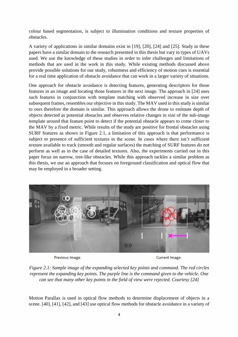
SURF features as shown in Figure 2.1, a limitation of this approach is that performance is

subject to presence of sufficient textures in the scene. In cases where there isn’t sufficient

texture available to track (smooth and regular surfaces) the matching of SURF features do not

perform as well as in the case of detailed textures. Also, the experiments carried out in this

paper focus on narrow, tree-like obstacles. While this approach tackles a similar problem as

this thesis, we use an approach that focuses on foreground classification and optical flow that

may be employed in a broader setting.

Figure 2.1: Sample image of the expanding selected key points and command. The red circles

represent the expanding key points. The purple line is the command given to the vehicle. One

can see that many other key points in the field of view were rejected. Courtesy [24]

Motion Parallax is used in optical flow methods to determine displacement of objects in a

scene. [40], [41], [42], and [43] use optical flow methods for obstacle avoidance in a variety of

5

scenarios but face limitations as flow estimation between consecutive frames is proportional to

the angle of the MAVs frontal direction. Due to this, objects moving towards the UAV during

flight don’t register a large degree of confidence as there may be small to no movement of

pixels when moving in a straight line. These methods do prove effective however for wall or

corridor following applications.

Another use of optical flow is in motion detection. Tracking markers to generate structure from

motion may be used by optical flow to estimate translation quantity of ergomotion [50]. Since

scenarios may exist where the environment is static and only the MAV camera moves, it

possible to segment objects using optical flow as objects closer to the camera appear to move

a greater distance between frames compared to objects further away. The accuracy of this

approach however is dependent on knowledge of the ergomotion between frames. Using optical

flow based motion models allows MAVs to navigate in indoor spaces as studied in [49] and

[51].

Bills et al [44] use an approach designed for indoor environments where there is uniformity in

structure properties. The paper makes use of edges and detects lines using Hough transform

and uses this information to classify the scene based on a trained classifier. While the paper

uses MAVs with a single camera, the proposed method in the paper allows the MAV to

navigate in indoor environments where such features can be used. Using these features, a

“confidence” value is determined based on line intersections crossing a visible vanishing point.

Based on this confidence value, the MAV adopts a control scheme to react accordingly to its

environment. When faced with an unknown environment; when confidence value is small; the

MAV enters an “unknown” state where it adopts defined exploration strategies. For indoor

applications, the method proposed in the paper may be applicable however for outdoor

situations scene regularity and line based cues are difficult to find making it difficult to train a

classifier as there may be constant changes in the scene. In contrast to this method, our approach

does not use any pre-existing training and learns the environment features during flight.

Celik et al [45] use an approach that exploits both lines and corner features detected in a scene.

Similar to the Hough transform method, the paper uses line information extracted from the

scene to determine the scene structure however, instead of running the method on the entire

scene, as Hough transform does, their method focuses only on scene parts where data exists.

The next proposition of the paper is using a human like range estimation method using the

height of the MAV and vanishing point of the scene. Using this information, the paper states

that it is possible to obtain the relative distance of an object in the scene following feature

points for its SLAM formulation. The paper uses a variation of optical flow as well for the

proposed Helix Bearing Algorithm to create a motion field to determine turning points in the

environment. This method too however is subject to camera capabilities and detection of strong

features in the scene to navigate successfully. The use of features and focus on relevant parts

of the scene is similar to our approach where the method focuses on select regions in the scene

instead of the entire scene as a whole. However estimating vanishing point may prove to be

difficult in natural environments due to irregularity in the scene.

Lee et al [46] propose a method with the use of MOPS (Multi-Scale-Oriented-Patches) and

SIFT feature descriptors to obtain three-dimensional information of the environment. MOPS,

similar to Harris corner detector, is a quick and accurate corner point matching method. Using

MOPS and SIFT, the paper attempts to reconstruct objects in 3D space where MOPS is used

6

to extract edge and corner information and SIFT used to detect the internal outline information

of an object. By combining these, a distinction between the outline and the inline of objects

can be determined using matching distance between frames. By listing cases between the

relationships of SIFT and MOPS features in the scene, it is possible to know the nature of

objects around when the UAV moves and construct a 3D map of the environment. While the

paper highlights experiments where they illustrate results from the proposed approach,

performance is subject to additional knowledge of flight test data. This however may not be

available for all use cases for this study in unknown environments.

Monocular cues used in the papers above ([44] [45] [46]) utilize information such as lines, and

scene regularities to detect proximity and location of obstacles however don’t perform well in

natural environments where such cues are challenging to find. Another limitation of these

methods is that monocular approaches may not find distance to collision directly however [48]

shows us that there exists a relationship between optical flow to time to collision which may

be exploited to determine immediate threat of obstacles. [16], [17] and [18] use motion cues to

estimate depth from motion and background subtraction to determine obstacles in a frontal

scene however face the issue of computational cost as well as robustness of detection. [19]

Uses a combination of appearance variation cues and optical flow for their approach to obstacle

detection. This method however is highly influenced by blob-based texture variations in the

environment and has limited performance in outdoor scenarios.

From literature above, we see several approaches to tacked obstacle avoidance in various

settings from indoor to outdoor but we also observe that these methods are subject to very

specific cases. Where some study uses scene regularities and geometric information in the

environment, this may not be the case in real applications especially in outdoor settings. Using

trained models help detect obstacles faster and accurately, results are conditioned to prior

knowledge of the obstacles or scenes. The approach presented in this thesis makes use of a

combination of background subtraction, optical flow, as well as depth estimation used in

individual studies to create a more robust obstacle avoidance system by taking the positive

points of existing methods.

7

3 General Methods Used

Our method uses background-foreground classification in the MAV flight environment and

uses this information to track feature points of potential obstacles. In order to achieve this, we

look at work in background segmentation proposed by papers [1], [2], [3], [4] and [5] where

the research focuses around creating a background model to generate foreground and

background masks for segmentation. Extensive study in feature detection in such environments

has been done in [11], [13], [14] and [15] where various methods for estimating optical flow

using salient features in frames are proposed. Using these concepts, we formalize general

methods used in this study below.

3.1 Background/Foreground classification

Background subtraction is a method in computer vision and image processing where an image

is classified into the background and the foreground. This is done to achieve a variety of

applications which require segmentation of concerned objects from a scene and filtering out

everything else. Background subtraction creates a model of the background and then segments

out everything that doesn’t belong to the background as foreground based on a spatial and

temporal setting. It’s can be seen as similar to detecting what objects are in the new image from

the old image. Once foreground objects are retrieved in the foreground mask, it is easy to

extract as well as localize the objects in the scene whether moving or stationary.

There are several approaches to achieve this such as Frame differencing [32], Mean Filtering

[33], Running Gaussian Average [34], and Mixture models [35]. The method we use in our

study is Background Subtraction using Mixtures of Gaussians by P. KaewTraKulPong and R.

Bowden.

The method proposed is in two parts where we first consider background modelling and then

maximising the expectation over the background Gaussian mixture model. The background is

modelled using an Adaptive Gaussian Mixture Model where each pixel in the scene is modelled

by K Gaussian distributions according to Grimson and Stauffer [37] and [38].

The probability of a pixel XN at time N belonging to a class is given as:

𝑝(𝑋𝑁) = ∑ 𝑤𝑗N(𝑥𝑁; 𝜃𝑗)𝐾𝑗=1 (1)

Where wk is the weight parameter of the kth Gaussian component. N(x:θk) is the normal

distribution component represented by:

N(x; 𝜃𝑘) = N(x; 𝜇𝑘, Ʃ𝑘) = 1

(2𝜋)𝐷2|Ʃ𝑘|

12

𝑒−12

(𝑥−𝜇𝑘)𝑇

Ʃ𝑘−1(𝑥−𝜇𝑘) (2)

8

Where µk is the mean and Ʃk=σk2I is the covariance of the kth component. The background B

is then modelled as:

𝐵 = 𝑎𝑟𝑔𝑚𝑖𝑛𝑏(∑ 𝑤𝑗 > 𝑇𝑏𝑗=1 ) (3)

Where T is the minimum fraction threshold of the background model. Here argminb is the

minimum prior probability that the background is in the scene. We then look at the update

equations for the Gaussian component that matches the test value as that is used by Grimson et

al:

�̂�𝑘𝑁+1 = (1 − 𝛼)�̂�𝑘

𝑁 + 𝛼�̂�(𝜔𝑘 |𝑋𝑁+1) (4)

�̂�𝑘𝑁+1 = (1 − 𝛼)�̂�𝑘

𝑁 + 𝜌𝑥𝑁+1 (5)

Ʃ̂𝑘𝑁+1 = (1 − 𝛼)Ʃ̂𝑘

𝑁 + 𝜌(𝑥𝑁+1 − �̂�𝑘𝑁+1)(𝑥𝑁+1 − �̂�𝑘

𝑁+1)𝑇 (6)

𝜌 = 𝛼N(𝑥𝑁+1; �̂�𝑘𝑁, Ʃ̂𝑘

𝑁) (7)

�̂�(𝜔𝑘 |𝑥𝑁+1) = {1 ; 𝑖𝑓 𝜔𝑘 𝑖𝑠 𝑡ℎ𝑒 𝑓𝑖𝑟𝑠𝑡 𝑚𝑎𝑡𝑐ℎ 𝐺𝑎𝑢𝑠𝑠𝑖𝑎𝑛 𝐶𝑜𝑚𝑝𝑜𝑛𝑒𝑛𝑡

0 ; 𝑜𝑡ℎ𝑒𝑟𝑤𝑖𝑠𝑒 (8)

Where ωk is the kth Gaussian component. 1/α defines the time constant that determines change

as learning rate. This update model however is incapable for complex background scenarios as

explained by [4]. Bowden et al [4] then propose online Expectation Maximization algorithms

to counter the issue of the method by Grimson et al [37] of slow convergence and inability to

account for minor changes in background by utilizing expected sufficient statistics update

equations and then switch to a window sampling method until the first L samples are processed

in order to allow faster convergence on a stable background model. The L-recent window

update equations prioritize over newer data leading to faster adaptation to changes in the

environment. The EM algorithms proposed by Bowden et al for expected sufficient statistics

are:

�̂�𝑘𝑁+1 = �̂�𝑘

𝑁 +1

𝑁+1(�̂�(𝜔𝑘|𝑥𝑁+1) − �̂�𝑘

𝑁) (9)

�̂�𝑘𝑁+1 = �̂�𝑘

𝑁 +𝑝(𝜔𝑘|𝑥𝑁+1)

∑ 𝑝(𝜔𝑘|𝑥𝑖)𝑁+1𝑖=1

(𝑥𝑁+1 − �̂�𝑘𝑁) (10)

Ʃ̂𝑘𝑁+1 = Ʃ̂𝑘

𝑁 +𝑝(𝜔𝑘|𝑥𝑁+1)

∑ 𝑝(𝜔𝑘|𝑥𝑖)𝑁+1𝑖=1

((𝑥𝑁+1 − �̂�𝑘𝑁)(𝑥𝑁+1 − �̂�𝑘

𝑁)𝑇 − Ʃ̂𝑘𝑁) (11)

And the L-recent window version is:

�̂�𝑘𝑁+1 = �̂�𝑘

𝑁 +1

𝐿(�̂�(𝜔𝑘|𝑥𝑁+1) − �̂�𝑘

𝑁) (12)

9

�̂�𝑘𝑁+1 = �̂�𝑘

𝑁 +1

𝐿

𝑝(𝜔𝑘|𝑥𝑁+1)

�̂�𝑘𝑁+1 (𝑥𝑁+1 − �̂�𝑘

𝑁) (13)

Ʃ̂𝑘𝑁+1 = Ʃ̂𝑘

𝑁 +1

𝐿

𝑝(𝜔𝑘|𝑥𝑁+1)

�̂�𝑘𝑁+1 ((𝑥𝑁+1 − �̂�𝑘

𝑁)(𝑥𝑁+1 − �̂�𝑘𝑁)𝑇 − Ʃ̂𝑘

𝑁) (14)

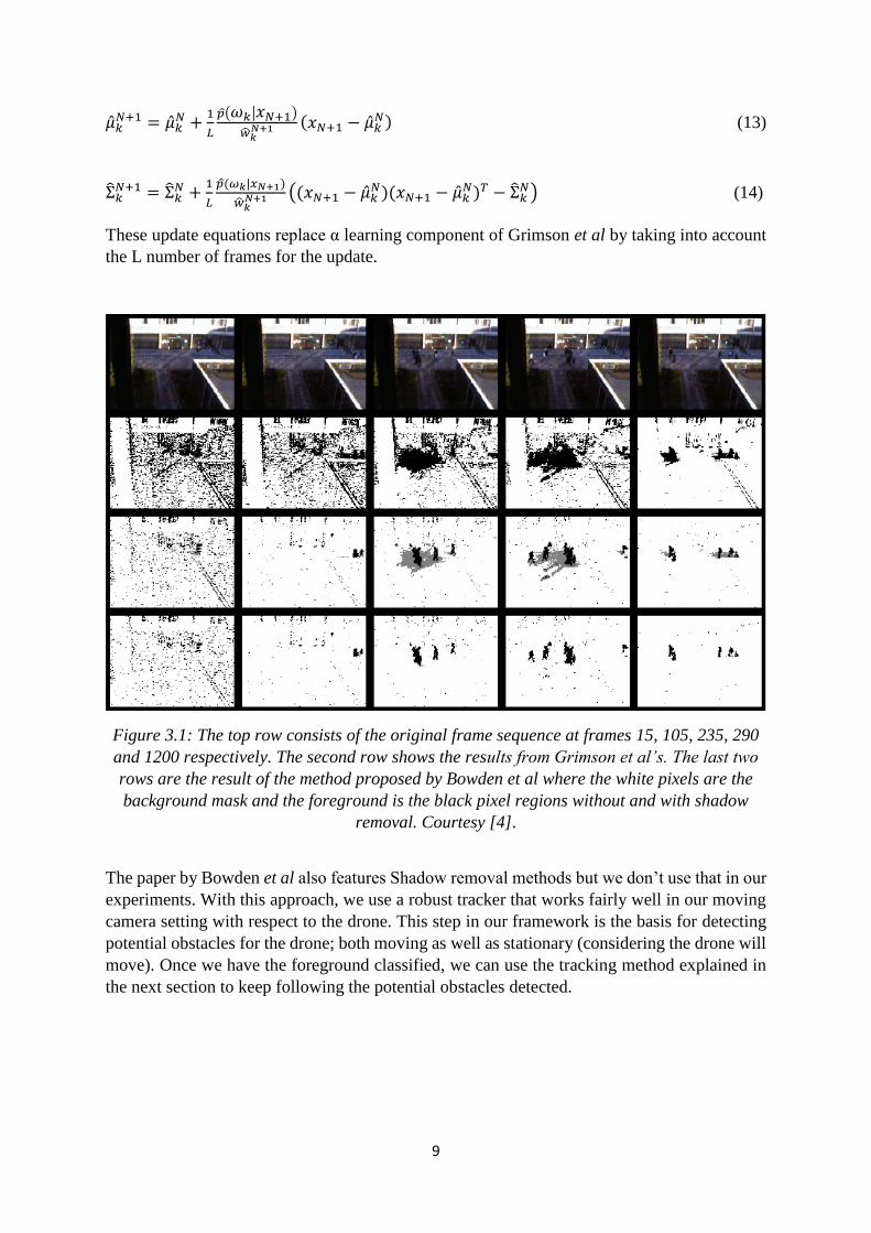
These update equations replace α learning component of Grimson et al by taking into account

the L number of frames for the update.

Figure 3.1: The top row consists of the original frame sequence at frames 15, 105, 235, 290

and 1200 respectively. The second row shows the results from Grimson et al’s. The last two

rows are the result of the method proposed by Bowden et al where the white pixels are the

background mask and the foreground is the black pixel regions without and with shadow

removal. Courtesy [4].

The paper by Bowden et al also features Shadow removal methods but we don’t use that in our

experiments. With this approach, we use a robust tracker that works fairly well in our moving

camera setting with respect to the drone. This step in our framework is the basis for detecting

potential obstacles for the drone; both moving as well as stationary (considering the drone will

move). Once we have the foreground classified, we can use the tracking method explained in

the next section to keep following the potential obstacles detected.

10

3.2 Tracking and Depth Classification

3.2.1 Feature detection

For feature detection we look at capturing good pixels to track. At this state, an apt choice of a

feature detector is essential. We look at classical the Harris Feature detector [12] with an

updated model by Shi and Tomasi [13]. A feature is an entity in an image (in our case) that

allows us to find matching points in two consecutive images so that we know the relation

between the two images. These features may also be seen as specific characteristics of an image

that “should” be present in the next image in the sequence which we can recognise easily. For

this feature to be recognised, it is essential that feature is uniquely recognisable in all images it

exists in. Features may exist in several ways such as corners, edges, colours, blobs to name a

few. Our interest in this research is on corner features and edge. Corner features are the point

of intersection between two edges and remain consistent in images unless occluded or skewed

by change in perspective or morphological properties of an object.

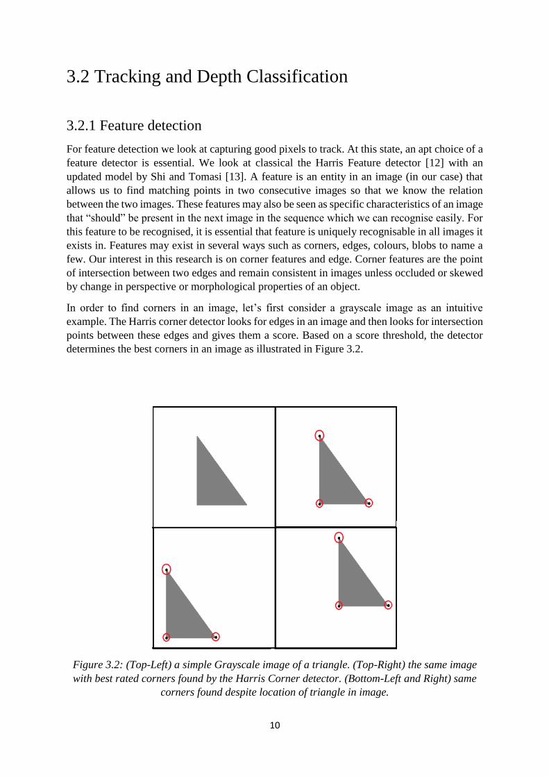
In order to find corners in an image, let’s first consider a grayscale image as an intuitive

example. The Harris corner detector looks for edges in an image and then looks for intersection

points between these edges and gives them a score. Based on a score threshold, the detector

determines the best corners in an image as illustrated in Figure 3.2.

Figure 3.2: (Top-Left) a simple Grayscale image of a triangle. (Top-Right) the same image

with best rated corners found by the Harris Corner detector. (Bottom-Left and Right) same

corners found despite location of triangle in image.

11

Based on the algorithm by Harris et al [12], we use a sliding window to go through the image

and calculate variations in intensity in that window using the equation:

𝐸(𝑢, 𝑣) = ∑ 𝑤(𝑥, 𝑦)[𝐼(𝑥 + 𝑢, 𝑦 + 𝑣) − 𝐼(𝑥, 𝑦)]2𝑥,𝑦 (15)

Where:

- w(x,y) is the window at position (x,y) in the image

- I(x,y) is the intensity at (x,y)

- I(x+u,y+v) is the intensity of the moved window w(x+u,y+v) where u is the window

shift in the x direction and v the shift in the y direction

Whenever the sliding window has a corner, we expect a large shift in intensity. We can then

represent the equation above to the form:

𝐸(𝑢, 𝑣) ≈ [𝑢 𝑣] 𝑀 [𝑢𝑣

] (16)

Where:

𝑀 = ∑ 𝑤(𝑥, 𝑦) [𝐼𝑥

2 𝐼𝑥𝐼𝑦

𝐼𝑥𝐼𝑦 𝐼𝑦2 ]𝑥,𝑦

Thus we have a score calculated for each window using the equation:

𝑅 = det(𝑀) − 𝑘(𝑡𝑟𝑎𝑐𝑒(𝑀))2 (17)

Where:

- det(M) = λ1 λ2

- trace(M) = λ1 + λ2

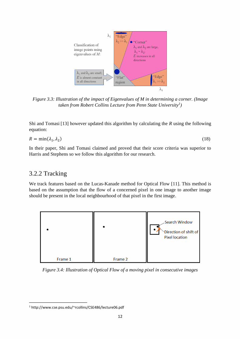
Therefore, we consider a window a corner if its R is greater than a threshold. The Eigenvalues

λ1 and λ2 represent a bidirectional axes of an ellipse for fitting a corner, edge or flat value in

the sliding window. An illustration of the impact of Eigenvalues of M is given in Figure 3.3

where classification is based on three cases:

- λ1 and λ2 are small, denoted a flat region

- λ1 > λ2 or λ1 < λ2, denotes an edge

- λ1 and λ2 are large, denotes a corner

12

Figure 3.3: Illustration of the impact of Eigenvalues of M in determining a corner. (Image

taken from Robert Collins Lecture from Penn State University1)

Shi and Tomasi [13] however updated this algorithm by calculating the R using the following

equation:

𝑅 = min(𝜆1, 𝜆2) (18)

In their paper, Shi and Tomasi claimed and proved that their score criteria was superior to

Harris and Stephens so we follow this algorithm for our research.

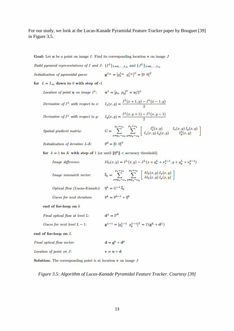
3.2.2 Tracking

We track features based on the Lucas-Kanade method for Optical Flow [11]. This method is

based on the assumption that the flow of a concerned pixel in one image to another image

should be present in the local neighbourhood of that pixel in the first image.

Figure 3.4: Illustration of Optical Flow of a moving pixel in consecutive images

1 http://www.cse.psu.edu/~rcollins/CSE486/lecture06.pdf

13

For our study, we look at the Lucas-Kanade Pyramidal Feature Tracker paper by Bouguet [39]

in Figure 3.5.

Figure 3.5: Algorithm of Lucas-Kanade Pyramidal Feature Tracker. Courtesy [39]

14

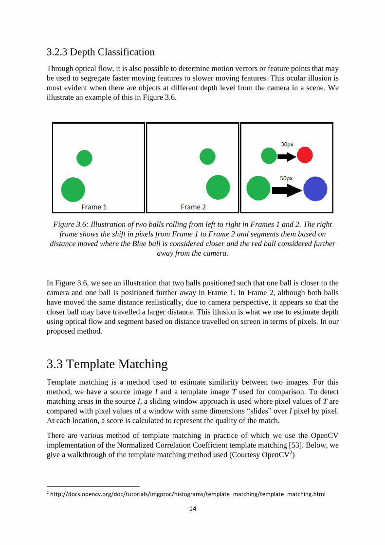
3.2.3 Depth Classification

Through optical flow, it is also possible to determine motion vectors or feature points that may

be used to segregate faster moving features to slower moving features. This ocular illusion is

most evident when there are objects at different depth level from the camera in a scene. We

illustrate an example of this in Figure 3.6.

Figure 3.6: Illustration of two balls rolling from left to right in Frames 1 and 2. The right

frame shows the shift in pixels from Frame 1 to Frame 2 and segments them based on

distance moved where the Blue ball is considered closer and the red ball considered further

away from the camera.

In Figure 3.6, we see an illustration that two balls positioned such that one ball is closer to the

camera and one ball is positioned further away in Frame 1. In Frame 2, although both balls

have moved the same distance realistically, due to camera perspective, it appears so that the

closer ball may have travelled a larger distance. This illusion is what we use to estimate depth

using optical flow and segment based on distance travelled on screen in terms of pixels. In our

proposed method.

3.3 Template Matching

Template matching is a method used to estimate similarity between two images. For this

method, we have a source image I and a template image T used for comparison. To detect

matching areas in the source I, a sliding window approach is used where pixel values of T are

compared with pixel values of a window with same dimensions “slides” over I pixel by pixel.

At each location, a score is calculated to represent the quality of the match.

There are various method of template matching in practice of which we use the OpenCV

implementation of the Normalized Correlation Coefficient template matching [53]. Below, we

give a walkthrough of the template matching method used (Courtesy OpenCV2)

2 http://docs.opencv.org/doc/tutorials/imgproc/histograms/template_matching/template_matching.html

15

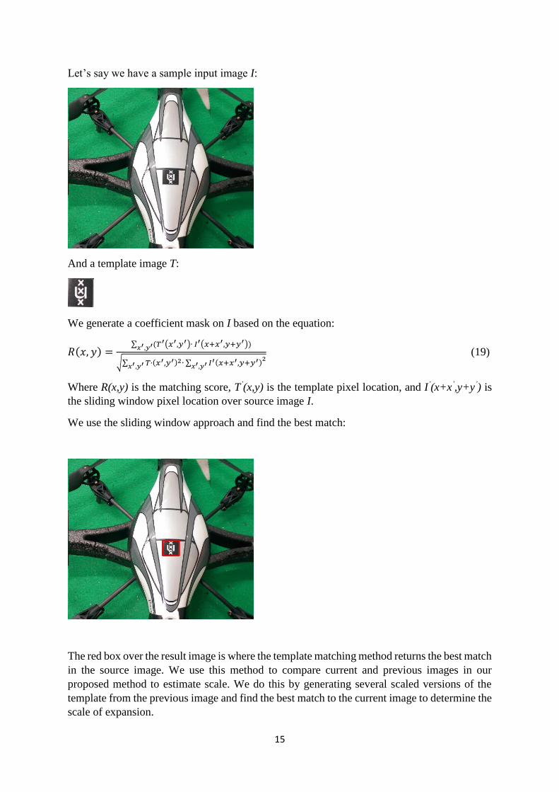
Let’s say we have a sample input image I:

And a template image T:

We generate a coefficient mask on I based on the equation:

𝑅(𝑥, 𝑦) =∑ (𝑇′(𝑥′,𝑦′)∙ 𝐼′(𝑥+𝑥′,𝑦+𝑦′))𝑥′,𝑦′

√∑ 𝑇,(𝑥′,𝑦′)2∙ ∑ 𝐼′(𝑥+𝑥′,𝑦+𝑦′)𝑥′,𝑦′

2𝑥′,𝑦′

(19)

Where R(x,y) is the matching score, T’(x,y) is the template pixel location, and I’(x+x’,y+y’) is

the sliding window pixel location over source image I.

We use the sliding window approach and find the best match:

The red box over the result image is where the template matching method returns the best match

in the source image. We use this method to compare current and previous images in our

proposed method to estimate scale. We do this by generating several scaled versions of the

template from the previous image and find the best match to the current image to determine the

scale of expansion.

16

4 Proposed Method

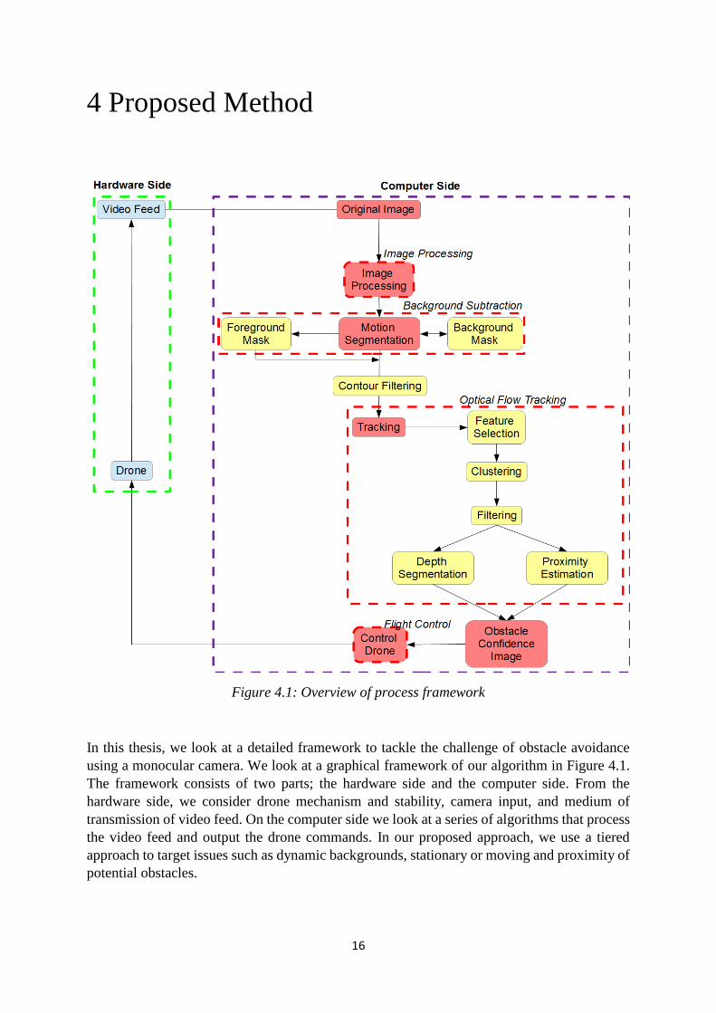
Figure 4.1: Overview of process framework

In this thesis, we look at a detailed framework to tackle the challenge of obstacle avoidance

using a monocular camera. We look at a graphical framework of our algorithm in Figure 4.1.

The framework consists of two parts; the hardware side and the computer side. From the

hardware side, we consider drone mechanism and stability, camera input, and medium of

transmission of video feed. On the computer side we look at a series of algorithms that process

the video feed and output the drone commands. In our proposed approach, we use a tiered

approach to target issues such as dynamic backgrounds, stationary or moving and proximity of

potential obstacles.

17

4.1 Background Subtraction

We use an existing implementation background subtraction using Mixtures of Gaussians3 as

explained in Section 3 in order to reduce the number of points generated in regions which are

not of interest in the environment using the foreground mask as well as its ability to cope with

dynamic backgrounds applicable to requirement. By focusing only on parts of a scene with a

significant degree of movement, we can eliminate a large number of unnecessary points to be

tracked in later stages. While this method is not a necessity in the framework, we see a

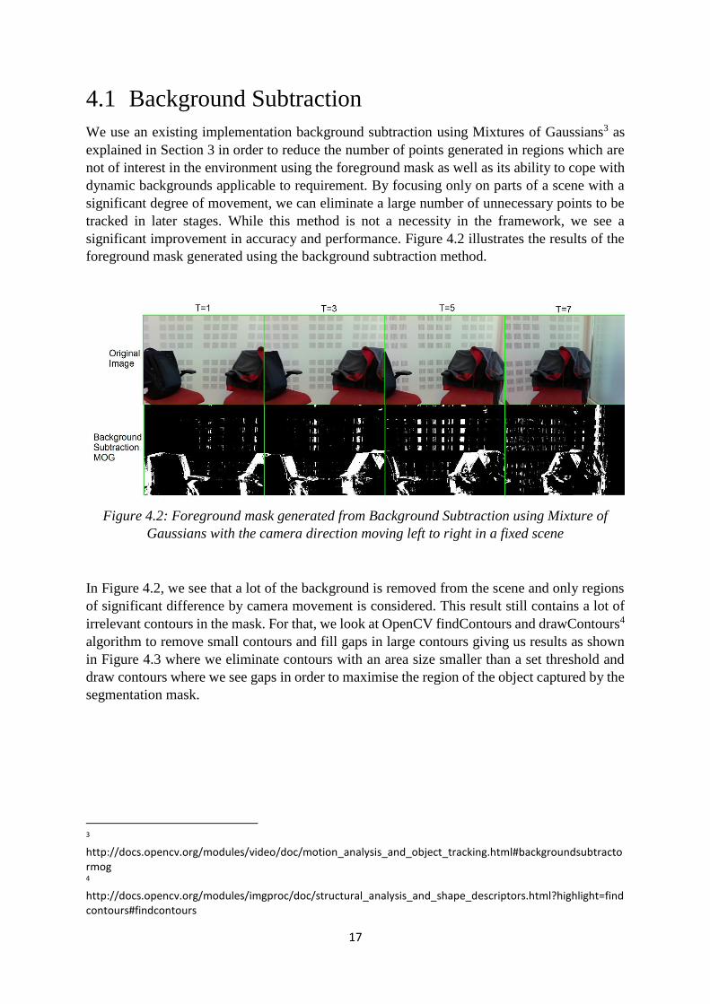
significant improvement in accuracy and performance. Figure 4.2 illustrates the results of the

foreground mask generated using the background subtraction method.

Figure 4.2: Foreground mask generated from Background Subtraction using Mixture of

Gaussians with the camera direction moving left to right in a fixed scene

In Figure 4.2, we see that a lot of the background is removed from the scene and only regions

of significant difference by camera movement is considered. This result still contains a lot of

irrelevant contours in the mask. For that, we look at OpenCV findContours and drawContours4

algorithm to remove small contours and fill gaps in large contours giving us results as shown

in Figure 4.3 where we eliminate contours with an area size smaller than a set threshold and

draw contours where we see gaps in order to maximise the region of the object captured by the

segmentation mask.

3 http://docs.opencv.org/modules/video/doc/motion_analysis_and_object_tracking.html#backgroundsubtractormog 4 http://docs.opencv.org/modules/imgproc/doc/structural_analysis_and_shape_descriptors.html?highlight=findcontours#findcontours

18

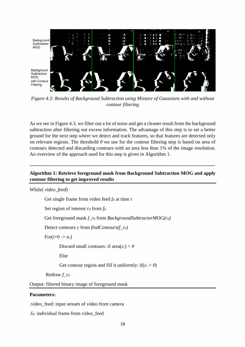
Figure 4.3: Results of Background Subtraction using Mixture of Gaussians with and without

contour filtering

As we see in Figure 4.3, we filter out a lot of noise and get a cleaner result from the background

subtraction after filtering out excess information. The advantage of this step is to set a better

ground for the next step where we detect and track features, so that features are detected only

on relevant regions. The threshold θ we use for the contour filtering step is based on area of

contours detected and discarding contours with an area less than 1% of the image resolution.

An overview of the approach used for this step is given in Algorithm 1.

___________________________________________________________________________

Algorithm 1: Retrieve foreground mask from Background Subtraction MOG and apply

contour filtering to get improved results

While( video_feed)

Get single frame from video feed f0 at time t

Set region of interest r0 from f0

Get foreground mask f_r0 from BackgroundSubtractorMOG(r0)

Detect contours c from findContours(f_r0)

For(i=0 -> nc)

Discard small contours: if area(ci) < θ

Else

Get contour region and fill it uniformly: if(ci > θ)

Redraw f_r0

Output: filtered binary image of foreground mask

Parameters:

.video_feed: input stream of video from camera

.f0: individual frame from video_feed

19

.t: time step

.r0: cropped region of interest from frame

.f_r0: foreground mask retrieved from Background Subtraction MOG implementation

.c: vector of contours detected from findContours implementation

.ci: ith contour value in cont vector

. θ: contour area threshold

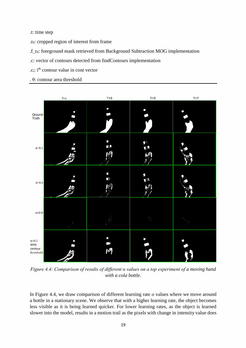
Figure 4.4: Comparison of results of different α values on a top experiment of a moving hand

with a cola bottle.

In Figure 4.4, we draw comparison of different learning rate α values where we move around

a bottle in a stationary scene. We observe that with a higher learning rate, the object becomes

less visible as it is being learned quicker. For lower learning rates, as the object is learned

slower into the model, results in a motion trail as the pixels with change in intensity value does

20

not learn as quickly. We use a learning rate of 0.1 for our method as it retains most properties

of the object in the scene and with our contour threshold extension, we note best results for our

case.

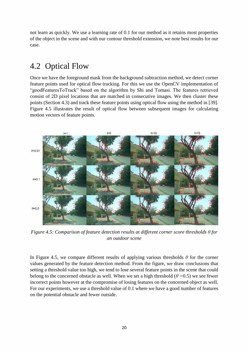
4.2 Optical Flow

Once we have the foreground mask from the background subtraction method, we detect corner

feature points used for optical flow tracking. For this we use the OpenCV implementation of

“goodFeaturesToTrack” based on the algorithm by Shi and Tomasi. The features retrieved

consist of 2D pixel locations that are matched in consecutive images. We then cluster these

points (Section 4.3) and track these feature points using optical flow using the method in [39].

Figure 4.5 illustrates the result of optical flow between subsequent images for calculating

motion vectors of feature points.

Figure 4.5: Comparison of feature detection results at different corner score thresholds θ for

an outdoor scene

In Figure 4.5, we compare different results of applying various thresholds θ for the corner

values generated by the feature detection method. From the figure, we draw conclusions that

setting a threshold value too high, we tend to lose several feature points in the scene that could

belong to the concerned obstacle as well. When we set a high threshold (θ =0.5) we see fewer

incorrect points however at the compromise of losing features on the concerned object as well.

For our experiments, we use a threshold value of 0.1 where we have a good number of features

on the potential obstacle and fewer outside.

21

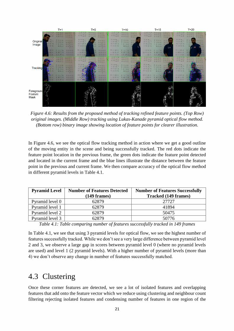
Figure 4.6: Results from the proposed method of tracking refined feature points. (Top Row)

original images. (Middle Row) tracking using Lukas-Kanade pyramid optical flow method.

(Bottom row) binary image showing location of feature points for clearer illustration.

In Figure 4.6, we see the optical flow tracking method in action where we get a good outline

of the moving entity in the scene and being successfully tracked. The red dots indicate the

feature point location in the previous frame, the green dots indicate the feature point detected

and located in the current frame and the blue lines illustrate the distance between the feature

point in the previous and current frame. We then compare accuracy of the optical flow method

in different pyramid levels in Table 4.1.

Pyramid Level Number of Features Detected

(149 frames)

Number of Features Successfully

Tracked (149 frames)

Pyramid level 0 62879 27727

Pyramid level 1 62879 41894

Pyramid level 2 62879 50475

Pyramid level 3 62879 50776

Table 4.1: Table comparing number of features successfully tracked in 149 frames

In Table 4.1, we see that using 3 pyramid levels for optical flow, we see the highest number of

features successfully tracked. While we don’t see a very large difference between pyramid level

2 and 3, we observe a large gap in scores between pyramid level 0 (where no pyramid levels

are used) and level 1 (2 pyramid levels). With a higher number of pyramid levels (more than

4) we don’t observe any change in number of features successfully matched.

4.3 Clustering

Once these corner features are detected, we see a lot of isolated features and overlapping

features that add onto the feature vector which we reduce using clustering and neighbour count

filtering rejecting isolated features and condensing number of features in one region of the

22

frame to limit computation load. For this, we implement our approach inspired by the method

in [52], where nearest neighbour chains are created between points and small clusters are made.

Then clusters are chained where each cluster is the nearest neighbour of the previous cluster.

This process is repeated until reaching a pair of clusters that are mutually nearest neighbours.

Our approach differs where we use a distance threshold d_θ instead of traversing through all

neighbour chains by sorting the all points from a common origin and providing a threshold to

the distance between neighbors n_θ. Algorithm 2 gives an overview of the clustering and

neighbour filtering method used to improve tracking results.

Algorithm 2: Cluster and group points based on Neighbouring features

Input: pn, d_θ, n_θ

Sort p based on distance to origin (top-left of image) to s_p

For(i=0 -> s_p.size)

Compute distance between s_pi and s_pi+1 to ds_p[i], s_p [1+1]

If(ds_p[i], s_p[1+1} < d_θ)

Add s_pi to c

If(ds_p [i], s_p [1+1] > d_θ)

If(c.size > n_θ)

Add c to f_pend

Clear c

Output: f_p

Parameters:

.p: vector of feature points detected

.d_θ: distance threshold to end cluster

.n_θ: number of neighbours to consider to keep cluster or discard

.s_p: sorted feature points based on distance to origin

. ds_p [i], s_p [1+1}: distance between s_p [i] and s_p [i+1]

.c: vector of clustered points

.f_p: vector of final points

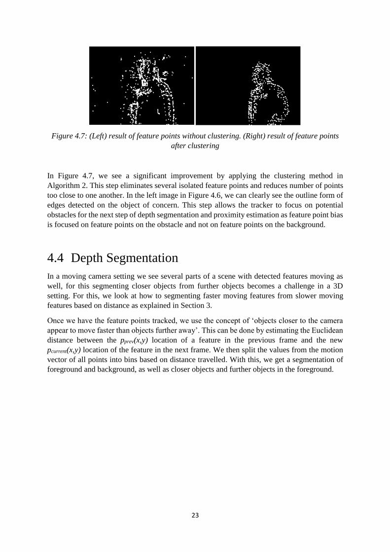
Once feature points are refined and trimmed, we see results of the method in Figure 4.7.

23

Figure 4.7: (Left) result of feature points without clustering. (Right) result of feature points

after clustering

In Figure 4.7, we see a significant improvement by applying the clustering method in

Algorithm 2. This step eliminates several isolated feature points and reduces number of points

too close to one another. In the left image in Figure 4.6, we can clearly see the outline form of

edges detected on the object of concern. This step allows the tracker to focus on potential

obstacles for the next step of depth segmentation and proximity estimation as feature point bias

is focused on feature points on the obstacle and not on feature points on the background.

4.4 Depth Segmentation

In a moving camera setting we see several parts of a scene with detected features moving as

well, for this segmenting closer objects from further objects becomes a challenge in a 3D

setting. For this, we look at how to segmenting faster moving features from slower moving

features based on distance as explained in Section 3.

Once we have the feature points tracked, we use the concept of ‘objects closer to the camera

appear to move faster than objects further away’. This can be done by estimating the Euclidean

distance between the pprev(x,y) location of a feature in the previous frame and the new

pcurrent(x,y) location of the feature in the next frame. We then split the values from the motion

vector of all points into bins based on distance travelled. With this, we get a segmentation of

foreground and background, as well as closer objects and further objects in the foreground.

24

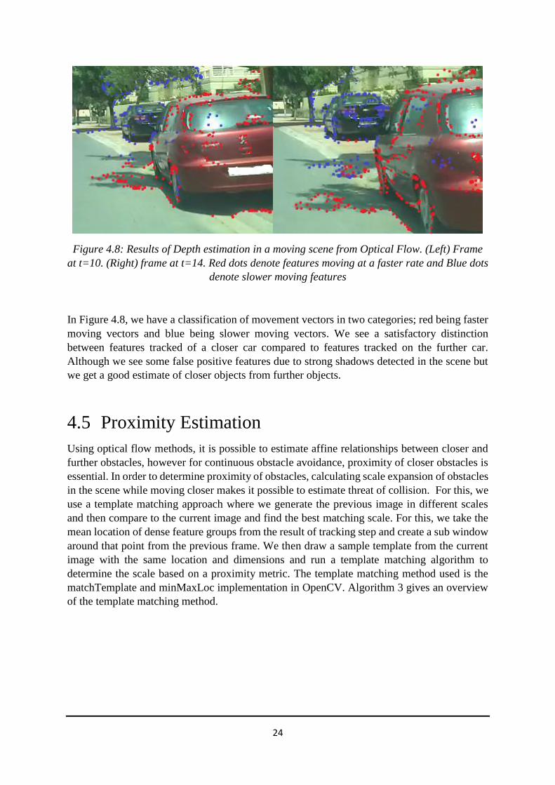
Figure 4.8: Results of Depth estimation in a moving scene from Optical Flow. (Left) Frame

at t=10. (Right) frame at t=14. Red dots denote features moving at a faster rate and Blue dots

denote slower moving features

In Figure 4.8, we have a classification of movement vectors in two categories; red being faster

moving vectors and blue being slower moving vectors. We see a satisfactory distinction

between features tracked of a closer car compared to features tracked on the further car.

Although we see some false positive features due to strong shadows detected in the scene but

we get a good estimate of closer objects from further objects.

4.5 Proximity Estimation

Using optical flow methods, it is possible to estimate affine relationships between closer and

further obstacles, however for continuous obstacle avoidance, proximity of closer obstacles is

essential. In order to determine proximity of obstacles, calculating scale expansion of obstacles

in the scene while moving closer makes it possible to estimate threat of collision. For this, we

use a template matching approach where we generate the previous image in different scales

and then compare to the current image and find the best matching scale. For this, we take the

mean location of dense feature groups from the result of tracking step and create a sub window

around that point from the previous frame. We then draw a sample template from the current

image with the same location and dimensions and run a template matching algorithm to

determine the scale based on a proximity metric. The template matching method used is the

matchTemplate and minMaxLoc implementation in OpenCV. Algorithm 3 gives an overview

of the template matching method.

25

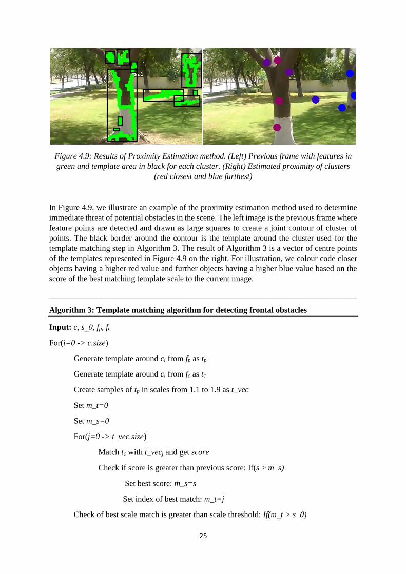
Figure 4.9: Results of Proximity Estimation method. (Left) Previous frame with features in

green and template area in black for each cluster. (Right) Estimated proximity of clusters

(red closest and blue furthest)

In Figure 4.9, we illustrate an example of the proximity estimation method used to determine

immediate threat of potential obstacles in the scene. The left image is the previous frame where

feature points are detected and drawn as large squares to create a joint contour of cluster of

points. The black border around the contour is the template around the cluster used for the

template matching step in Algorithm 3. The result of Algorithm 3 is a vector of centre points

of the templates represented in Figure 4.9 on the right. For illustration, we colour code closer

objects having a higher red value and further objects having a higher blue value based on the

score of the best matching template scale to the current image.

___________________________________________________________________________

Algorithm 3: Template matching algorithm for detecting frontal obstacles

Input: c, s_θ, fp, fc

For(i=0 -> c.size)

Generate template around ci from fp as tp

Generate template around ci from fc as tc

Create samples of tp in scales from 1.1 to 1.9 as t_vec

Set m_t=0

Set m_s=0

For(j=0 -> t_vec.size)

Match tc with t_vecj and get score

Check if score is greater than previous score: If(s > m_s)

Set best score: m_s=s

Set index of best match: m_t=j

Check of best scale match is greater than scale threshold: If(m_t > s_θ)

26

Add location of that cluster to obstacle location vector:

o_vecend = ci

Output: o_vec

Parameters:

.c: vector of midpoints of feature point clusters

.s_θ: scale threshold for obstacle threat

.fp: previous video frame

.fc: current video frame

.tp: template around cluster point ci in fp

.tc: template around cluster point ci in fc

.t_vec: vector of enlarged scales of tp in 9 sizes

.s: matching score between tc and t_vecj

.m_t: scale at which best match is found

.m_s: score of best match

.o_vec: vector of locations of all probable obstacle threats

27

5 Experiments and Results

5.1 Tools

For our experiments, we use a variety of tools for our experiments. We use the AR Drone by

Parrot SA for our experiments, OpenCV in C++ as our core processing library, and ROS with

ardrone_autonomy driver to bridge communication between the computer and the drone.

5.1.1 Robot Operating System (ROS)

The experiments presented in this thesis uses the Robot Operating System (ROS) software

framework as a bridge between the robot we use, in our case the A.R. Drone by Parrot S.A.

and a computer where ROS is loaded with the proposed method. ROS was originally developed

in 2007 by the Stanford Artificial Intelligence Laboratory as an operating system as

functionality for a variety of robots and hardware.

ROS provides several operating system services such as hardware abstraction, process

management and message passing, packet management as well as implementation of

commonly used functionality for devices. ROS is released under terms of BSD license5 and is

freely available as open source software for commercial as well as research use.

We use ROS in our application in order to bridge communication between the processing

computer and the drone. The choice of using ROS is influenced by availability of drivers and

support specific for the AR Drone. While ROS offers several features for message passing,

monitoring, and visualization tools, we utilize only the node framework and message passing

system to bridge communication.

5.1.2 OpenCV

OpenCV is a popular computer vision library of programming functions focused around real-

time computer vision applications. OpenCV was officially launched in 1999 as an Intel

Research Initiative initially in C programming language and later in C++ and Python

programming language as a cross platform suite. OpenCV as a BSD license and is freely

available as open source for both commercial as well as research use.

OpenCV has several state of the art implementation of popular computer vision algorithms and

applications. The functionality we use in our application are as:

Image processing

Video analysis

2D features framework

Object detection

5 http://www.linfo.org/bsdlicense.html

28

Machine learning

Clustering and Search in multi-dimensional spaces

OpenCV is also supported by several tutorials and detailed documentation on its website6. A

large part of the research utilizes this library which makes it a suitable choice due to the nature

of the research and the fact that it is freely available and widely used with several official7 as

well as unofficial forums.

5.1.3 Parrot A.R. Drone

We consider a quad-rotor helicopter that is both small enough to be used in indoor as well as

outdoor environments for our experiments. The small size a design of quad-rotors allow agile

and responsive flight and easy maintenance.

The Parrot A.R. Drone (Figure 5.1) is a popular and affordable quad-rotor that may be bought

off the shelf in hobby stores and has good applicability in our study. The design of this specific

drone allows for easy maintenance with replaceable parts. A significant advantage of using off-

the-shelf drones is specific features of on-bard stabilization and easy control design that allows

us to focus on developing intelligent applications without focusing on developing hardware.

Below we list some of the useful features that come factory-fitted with the drone:

Forward and bottom facing cameras: The drone comes equipped with two cameras; a

forward facing camera and a bottom facing camera. Both cameras provide live video

streaming to the control device.

Auto stabilization: The drone has an excellent on-board stabilization system that uses

rotors, a gyroscope as well as the bottom camera for improved stabilization

Wireless connectivity: The drone can easily be connected to wireless devices such as

smart phones and tablets (iOS and Android from their respective app stores), as well as

computers with the corresponding drivers (example; ardrone_autonomy).

6 http://docs.opencv.org/ 7 http://answers.opencv.org/questions/

29

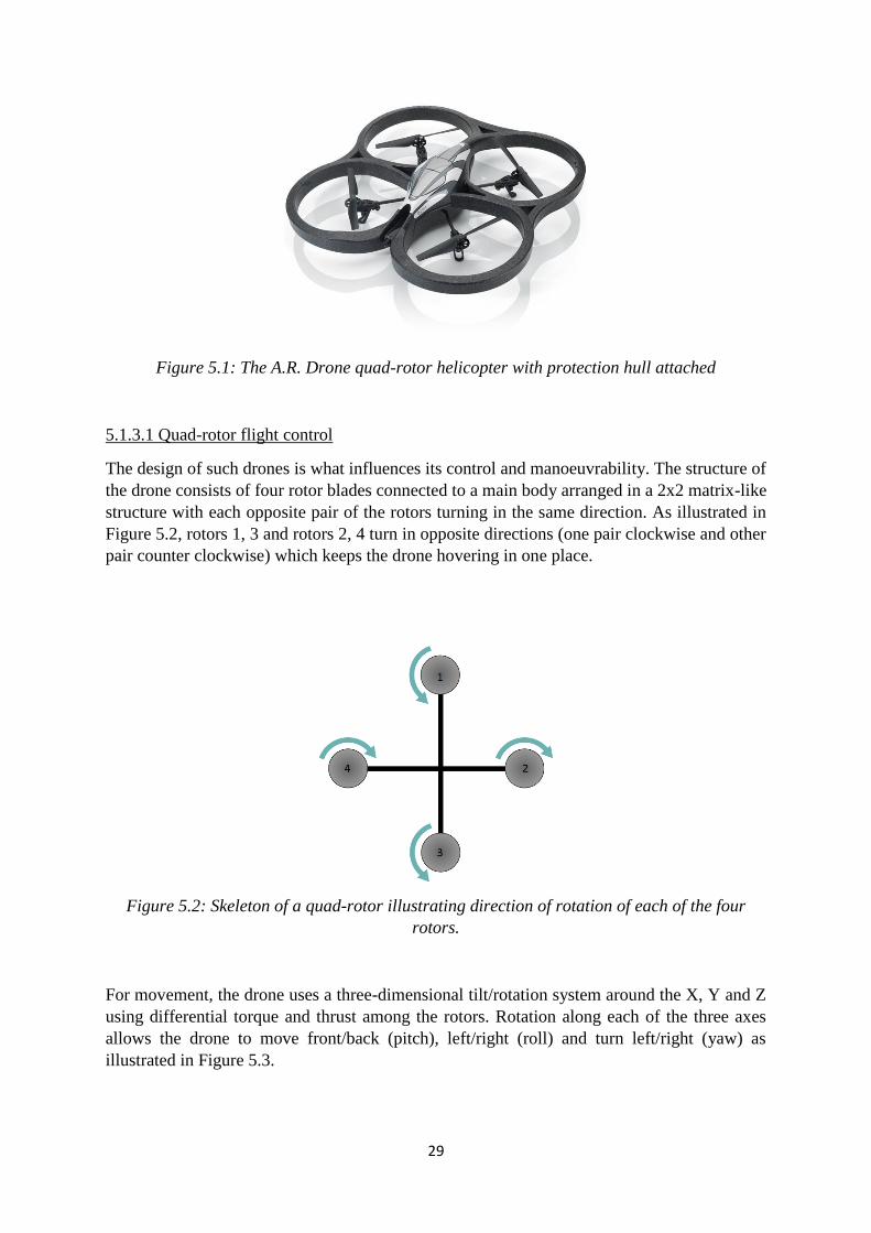
Figure 5.1: The A.R. Drone quad-rotor helicopter with protection hull attached

5.1.3.1 Quad-rotor flight control

The design of such drones is what influences its control and manoeuvrability. The structure of

the drone consists of four rotor blades connected to a main body arranged in a 2x2 matrix-like

structure with each opposite pair of the rotors turning in the same direction. As illustrated in

Figure 5.2, rotors 1, 3 and rotors 2, 4 turn in opposite directions (one pair clockwise and other

pair counter clockwise) which keeps the drone hovering in one place.

Figure 5.2: Skeleton of a quad-rotor illustrating direction of rotation of each of the four

rotors.

For movement, the drone uses a three-dimensional tilt/rotation system around the X, Y and Z

using differential torque and thrust among the rotors. Rotation along each of the three axes

allows the drone to move front/back (pitch), left/right (roll) and turn left/right (yaw) as

illustrated in Figure 5.3.

30

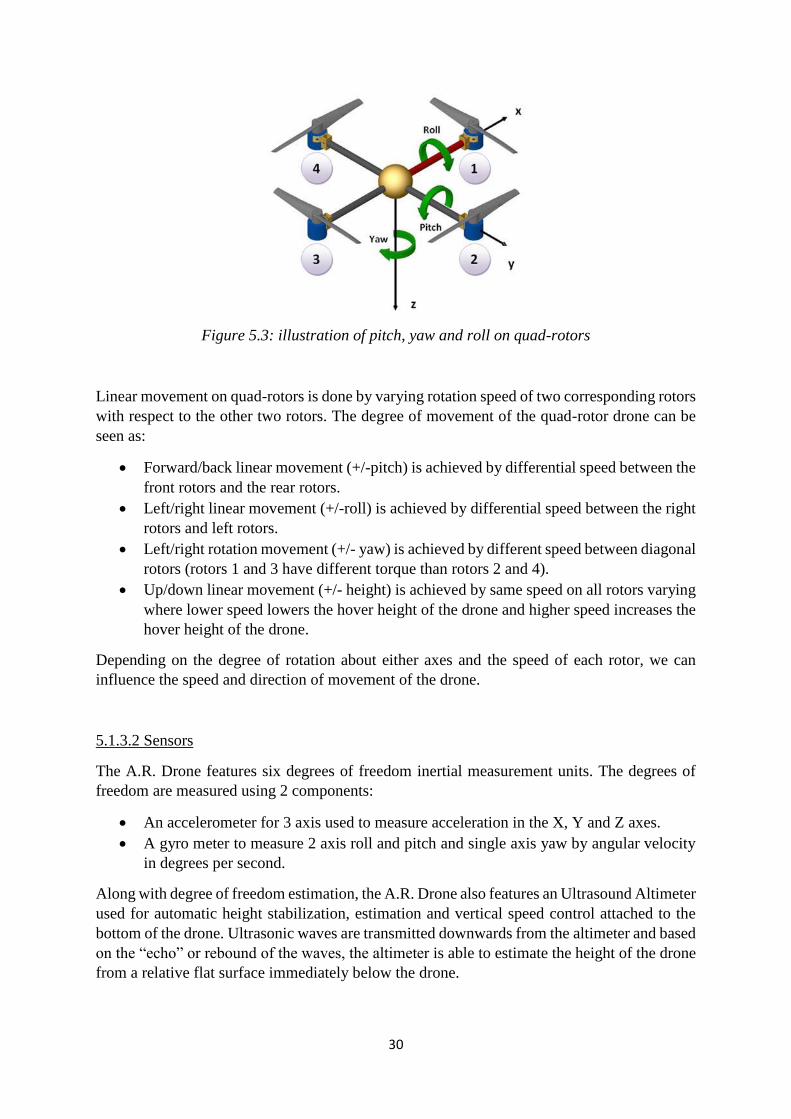
Figure 5.3: illustration of pitch, yaw and roll on quad-rotors

Linear movement on quad-rotors is done by varying rotation speed of two corresponding rotors

with respect to the other two rotors. The degree of movement of the quad-rotor drone can be

seen as:

Forward/back linear movement (+/-pitch) is achieved by differential speed between the

front rotors and the rear rotors.

Left/right linear movement (+/-roll) is achieved by differential speed between the right

rotors and left rotors.

Left/right rotation movement (+/- yaw) is achieved by different speed between diagonal

rotors (rotors 1 and 3 have different torque than rotors 2 and 4).

Up/down linear movement (+/- height) is achieved by same speed on all rotors varying

where lower speed lowers the hover height of the drone and higher speed increases the

hover height of the drone.

Depending on the degree of rotation about either axes and the speed of each rotor, we can

influence the speed and direction of movement of the drone.

5.1.3.2 Sensors

The A.R. Drone features six degrees of freedom inertial measurement units. The degrees of

freedom are measured using 2 components:

An accelerometer for 3 axis used to measure acceleration in the X, Y and Z axes.

A gyro meter to measure 2 axis roll and pitch and single axis yaw by angular velocity

in degrees per second.

Along with degree of freedom estimation, the A.R. Drone also features an Ultrasound Altimeter

used for automatic height stabilization, estimation and vertical speed control attached to the

bottom of the drone. Ultrasonic waves are transmitted downwards from the altimeter and based

on the “echo” or rebound of the waves, the altimeter is able to estimate the height of the drone

from a relative flat surface immediately below the drone.

31

The A.R. Drone also features two cameras, one facing forward and one downward both of

which support live streaming. The forward camera is primarily used for piloting the drone by

transmitting live video feed to the controlling device. The bottom camera serves three purposes;

to see what is below the drone, horizontal stabilization as well as estimating the velocity of the

drone.

5.1.3.3 On-board Intelligence

The drone comes factory installed with several on-board intelligence functions. A primary

example of the drone’s on-board intelligence is the flight stability procedure which makes use

of all sensors and cameras to maintain the drones position, awareness and state estimation. As

the drone’s on-board software is closed source and not publicly documented by the

manufacturer, we don’t alter/modify this system and use it as-is.

In our experiments, taking the on-board stability, estimation and controls as-is and without

alteration, we use only the front camera live feed for processing. Detailed Documentation for

the A.R. Drone is available on the official Parrot S.A. website8.

5.1.4 A.R. Drone Driver for ROS

At the time of this research, ROS did not have any built in driver for the A.R. Drone 2.0 so for

this we use a third-party driver specifically tailored to the drone we will be experimenting on

in this research. Ardrone_autonomy9 is a ROS driver with copyright and proprietary rights

based on the official AR-Drone SDK 2.010 with BSD license for other parts of implementation

and is developed by Simon Fraser University by Mani Monajjemi11 among other contributors.

The driver provides several control parameters for the drone suited to our application such as:

Three-dimensional rotation along the X(left/right tilt), Y(forward/backward tilt) and

Z(orientation) axes

Magnetometer readings along X, Y and Z axes

Linear velocity along X, Y and Z axes

Linear acceleration along X, Y and Z axes

Front and bottom cameras

Take-off and landing

Flat trim (a service that calibrates the drone based on rotation estimates assuming it is

on a flat surface)

8 http://ardrone2.parrot.com/ 9 https://github.com/AutonomyLab/ardrone_autonomy 10 https://projects.ardrone.org/ 11 http://sfu.ca/~mmonajje

32

These parameters provide a good control of the drone from the software side of the experiment

for the pilot controller which will be discussed later. The driver package also comes with

several tutorials and documentation on several official and unofficial forums.

5.1.5 PC Configuration

The video feed from the AR. Drone is processed entirely on a laptop connected via Wi-Fi in

close unobstructed proximity. The specification of the laptop are:

Processor: Intel Core i7 quad-core processor @1.73Ghz

Memory: 8GB DDR3 RAM

Operating System: Ubuntu 12.04

Wireless card: Intel WiFi Link 5300 AGN

5.2 General Experiments

In this section, we look at experiments of our general methods with the proposed extensions in

a number of toy experiments. Experiments carried out are using only the video feed of a drone

in stationary and moving settings. All flight experiments are carried out in Dubai, United Arab

Emirates where we see consistent climate conditions throughout the duration of our

experiments.

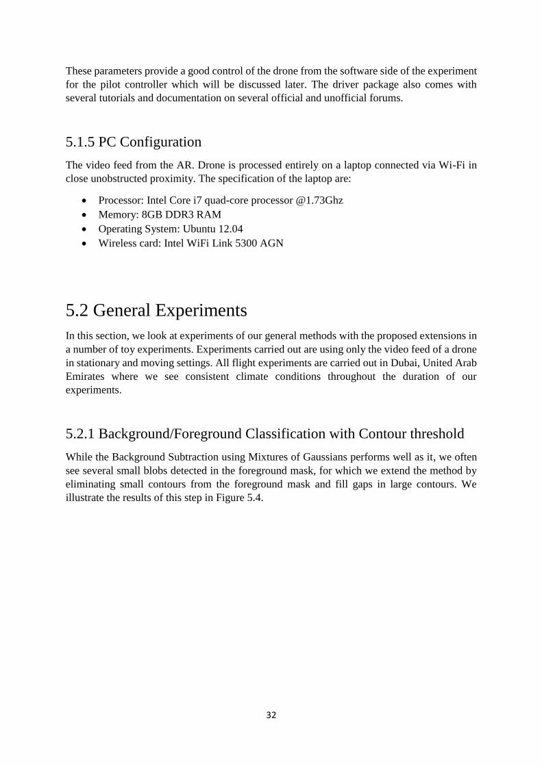
5.2.1 Background/Foreground Classification with Contour threshold

While the Background Subtraction using Mixtures of Gaussians performs well as it, we often

see several small blobs detected in the foreground mask, for which we extend the method by

eliminating small contours from the foreground mask and fill gaps in large contours. We

illustrate the results of this step in Figure 5.4.

33

Figure 5.4: Results of the proposed extension on the standard OpenCV implementation of

background subtraction using MOG

Discussion: In Figure 5.4, we have a setting where obstacles are stationary and the camera is

moving. The first and second row show the original image and ground truth respectively. The

second row shows the result of our algorithm where we extend the background subtraction with

MOG algorithm with contour thresholds. The last row shows results of the standard OpenCV

background subtraction MOG implementation where we can see a lot of the texture of the

background being classified as foreground. To evaluate the error rate between the results of

using background subtraction MOG with and without the contour threshold step, we compare

the result of each image of each method to the ground truth in a pixel-wise comparison where

matching pixels return a true value and un-matching pixels return a false value and estimate

the error rate in Table 5.1.

Method Error (avg. over 50

frames)

Background Subtraction with MOG and

cluster threshold

18.59

Background Subtraction with MOG 23.995

Table 5.1: Table comparing pixel-wise average error rate of the proposed method and the

OpenCV implementation of Background Subtraction MOG

34

In Table 5.1, we compare pixel-wise accuracy of both methods and average it over 50 frames.

We see that the proposed method performs significantly better looking at the error rate as well

as the results in Figure 5.6. Our method filters out small background texture and removes a lot

of trail or drag of the objects in the foreground mask caused when the camera moves. With

this, we see that by using the cluster threshold feature, we have significantly fewer regions to

detect feature points from and thereby increasing accuracy for following processes.

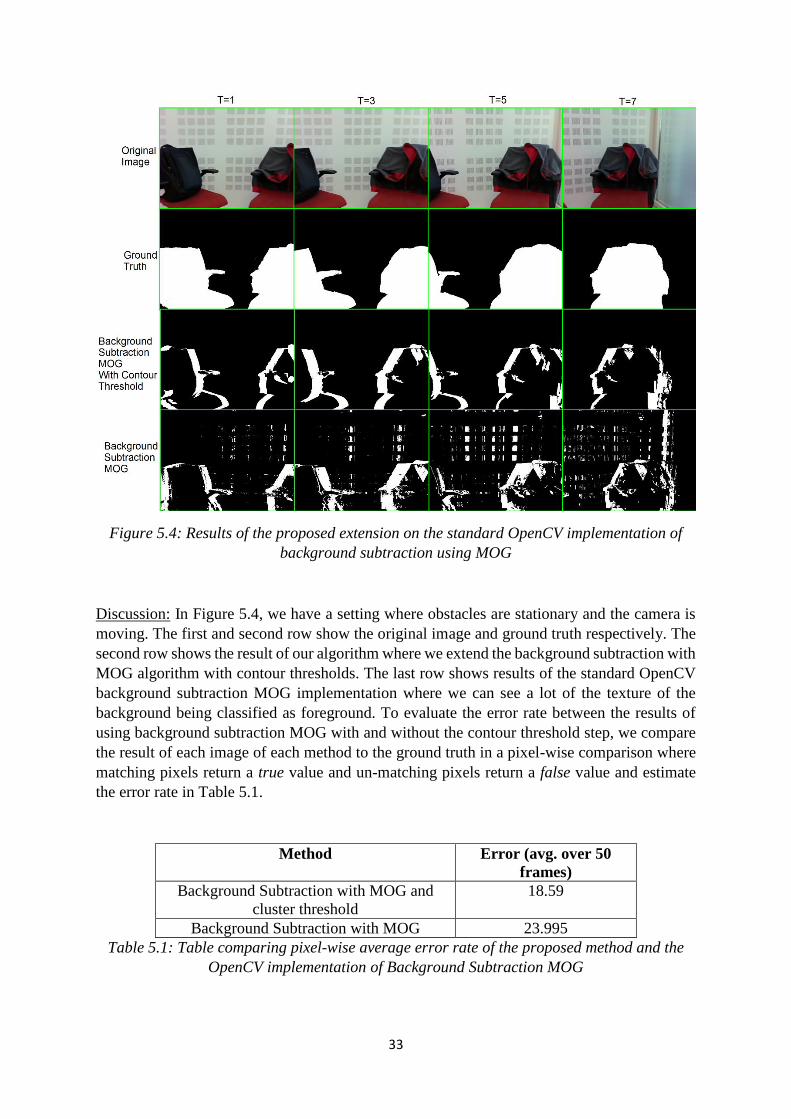
5.2.2 Feature selection and Tracking

For testing the tracking and feature selection module, we use the same environment setting as

earlier where we use the results of the motion segmentation step as our input and track moving

obstacles in the scene. We establish three settings for our experiments and compare the results

in terms of frame-rate and number of features accurately/inaccurately tracked. Figures 5.6, 5.7

and 5.8 show the results in settings; tracking with background subtraction, tracking without

background subtraction and tracking without feature point clustering respectively.

Figure 5.5: Results from the proposed method of tracking motion input from the background

subtraction module previously and clustering feature points. (Top row) original images,

(middle row) tracking using Lucas-Kanade pyramid optical flow algorithm and (bottom row)

foreground feature mask generated after tracking, clustering and segmentation

35

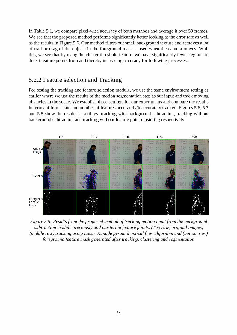
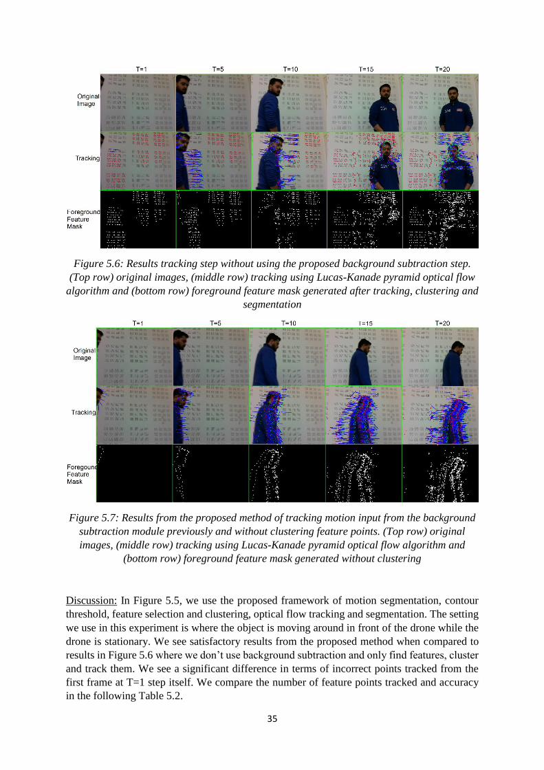
Figure 5.6: Results tracking step without using the proposed background subtraction step.

(Top row) original images, (middle row) tracking using Lucas-Kanade pyramid optical flow

algorithm and (bottom row) foreground feature mask generated after tracking, clustering and

segmentation

Figure 5.7: Results from the proposed method of tracking motion input from the background

subtraction module previously and without clustering feature points. (Top row) original

images, (middle row) tracking using Lucas-Kanade pyramid optical flow algorithm and

(bottom row) foreground feature mask generated without clustering

Discussion: In Figure 5.5, we use the proposed framework of motion segmentation, contour

threshold, feature selection and clustering, optical flow tracking and segmentation. The setting

we use in this experiment is where the object is moving around in front of the drone while the

drone is stationary. We see satisfactory results from the proposed method when compared to

results in Figure 5.6 where we don’t use background subtraction and only find features, cluster

and track them. We see a significant difference in terms of incorrect points tracked from the

first frame at T=1 step itself. We compare the number of feature points tracked and accuracy

in the following Table 5.2.

36

Method Number of

Points (avg. 50

frames)

Correct (avg.

50 frames)

Incorrect (avg.

50 frames)

Frame-rate

(avg. 50

frames)

BS-MOG + LK-

clust

982 952 30 15

LK-clust 1624 1098 526 4

Table 5.2: Comparison chart between numbers of points accurately tracked between the

proposed method and standalone optical flow tracking

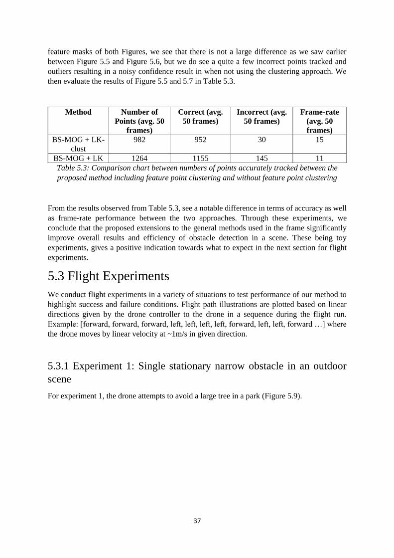
From Table 5.2, we draw conclusions that due to the segmentation step not used before finding

feature points, there are lots of corners in the background that classify as feature points and are

tracked constantly. The background subtraction step allows the result from feature detection to

be focused resulting in accuracy as well as lower computation power when we calculate the

average frame-rate. Even with the same feature selection settings, we see a considerable

difference in terms of accuracy between the proposed method and the stand-alone optical flow

method when we compare the foreground feature mask of both in Figure 5.5 and 5.6

respectively. While the confidence images in Figure 5.5 segment the object from the scene

fairy well, we see a lot of random points and arbitrary shifting features in the confidence images

in Figure 5.6.

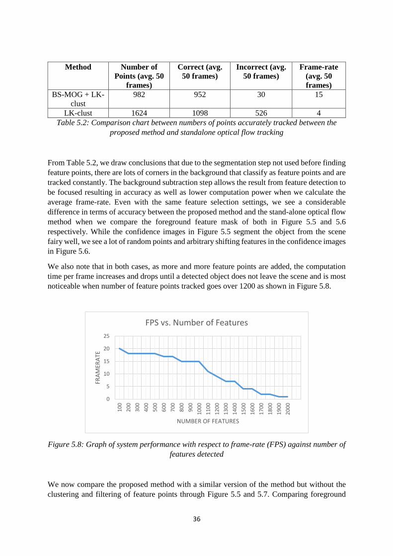
We also note that in both cases, as more and more feature points are added, the computation

time per frame increases and drops until a detected object does not leave the scene and is most

noticeable when number of feature points tracked goes over 1200 as shown in Figure 5.8.

Figure 5.8: Graph of system performance with respect to frame-rate (FPS) against number of

features detected

We now compare the proposed method with a similar version of the method but without the

clustering and filtering of feature points through Figure 5.5 and 5.7. Comparing foreground

0

5

10

15

20

25

10

0

20

0

30

0

40

0

50

0

60

0

70

0

80

0

90

0

10

00

11

00

12

00

13

00

14

00

15

00

16

00

17

00

18

00

19

00

20

00

FRA

MER

ATE

NUMBER OF FEATURES

FPS vs. Number of Features

37

feature masks of both Figures, we see that there is not a large difference as we saw earlier

between Figure 5.5 and Figure 5.6, but we do see a quite a few incorrect points tracked and

outliers resulting in a noisy confidence result in when not using the clustering approach. We

then evaluate the results of Figure 5.5 and 5.7 in Table 5.3.

Method Number of

Points (avg. 50

frames)

Correct (avg.

50 frames)

Incorrect (avg.

50 frames)

Frame-rate

(avg. 50

frames)

BS-MOG + LK-

clust

982 952 30 15

BS-MOG + LK 1264 1155 145 11

Table 5.3: Comparison chart between numbers of points accurately tracked between the

proposed method including feature point clustering and without feature point clustering

From the results observed from Table 5.3, see a notable difference in terms of accuracy as well

as frame-rate performance between the two approaches. Through these experiments, we

conclude that the proposed extensions to the general methods used in the frame significantly

improve overall results and efficiency of obstacle detection in a scene. These being toy

experiments, gives a positive indication towards what to expect in the next section for flight

experiments.

5.3 Flight Experiments

We conduct flight experiments in a variety of situations to test performance of our method to

highlight success and failure conditions. Flight path illustrations are plotted based on linear

directions given by the drone controller to the drone in a sequence during the flight run.

Example: [forward, forward, forward, left, left, left, left, forward, left, left, forward …] where

the drone moves by linear velocity at ~1m/s in given direction.

5.3.1 Experiment 1: Single stationary narrow obstacle in an outdoor

scene

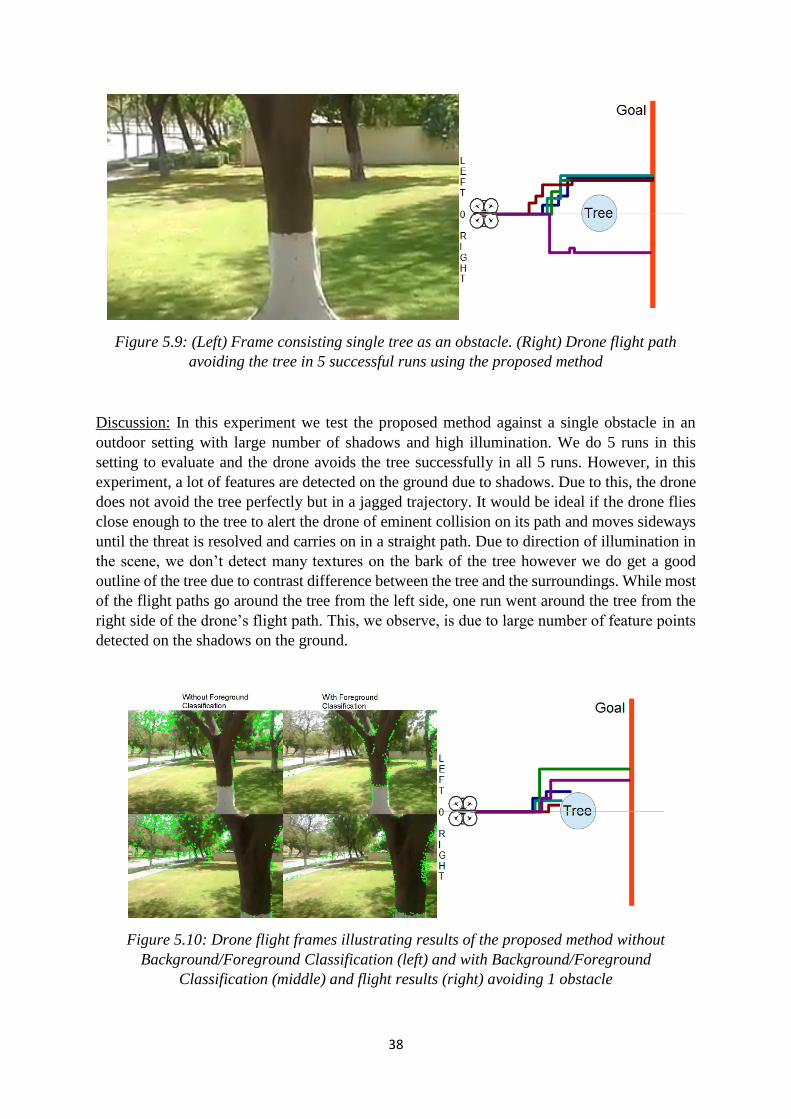
For experiment 1, the drone attempts to avoid a large tree in a park (Figure 5.9).

38

Figure 5.9: (Left) Frame consisting single tree as an obstacle. (Right) Drone flight path

avoiding the tree in 5 successful runs using the proposed method

Discussion: In this experiment we test the proposed method against a single obstacle in an

outdoor setting with large number of shadows and high illumination. We do 5 runs in this

setting to evaluate and the drone avoids the tree successfully in all 5 runs. However, in this

experiment, a lot of features are detected on the ground due to shadows. Due to this, the drone

does not avoid the tree perfectly but in a jagged trajectory. It would be ideal if the drone flies

close enough to the tree to alert the drone of eminent collision on its path and moves sideways

until the threat is resolved and carries on in a straight path. Due to direction of illumination in

the scene, we don’t detect many textures on the bark of the tree however we do get a good

outline of the tree due to contrast difference between the tree and the surroundings. While most

of the flight paths go around the tree from the left side, one run went around the tree from the

right side of the drone’s flight path. This, we observe, is due to large number of feature points

detected on the shadows on the ground.

Figure 5.10: Drone flight frames illustrating results of the proposed method without

Background/Foreground Classification (left) and with Background/Foreground

Classification (middle) and flight results (right) avoiding 1 obstacle

39

In order to illustrate the impact of the background/foreground classification in our proposed

method, we look at sample screenshots of drone flight with and without background subtraction

in Figure 5.10. In Figure 5.10, we see a lot of feature points (green circles) detected in the

background of the scene and not many on the obstacle of concern. Due to this, there is a very

strong influence of feature points detected on trees at the back which affect the drone controller

decisions. Using the proposed method with background/foreground classification, we get a lot

more contours on the obstacle of concern and much fewer in the background. Due to which,

the drone controller decisions are more accurate avoiding the obstacle in the scene, results of

which are illustrated on the right in Figure 5.10. From the flight results, we observe that 3 runs

fail (blue, red, and turquoise) as best features are detected in the trees in the background and

not many detected on the obstacle tree. For the 2 successful runs (green and purple), we see the

few features detected on the tree providing a small bias to the drone controller to move left and

avoid the obstacle. Overall results for average number of total, correct and incorrect features

detected over total number of frames are shown in table 5.4.

Method Number of

Features

Correct Features Incorrect Features

Proposed method 467 382 85

Proposed method

w/o BG/FG

classification

1539 126 1413

Table 5.4: Table of comparison of number of correct and incorrect features detected between

proposed method with and without background/foreground classification for a single narrow

obstacle

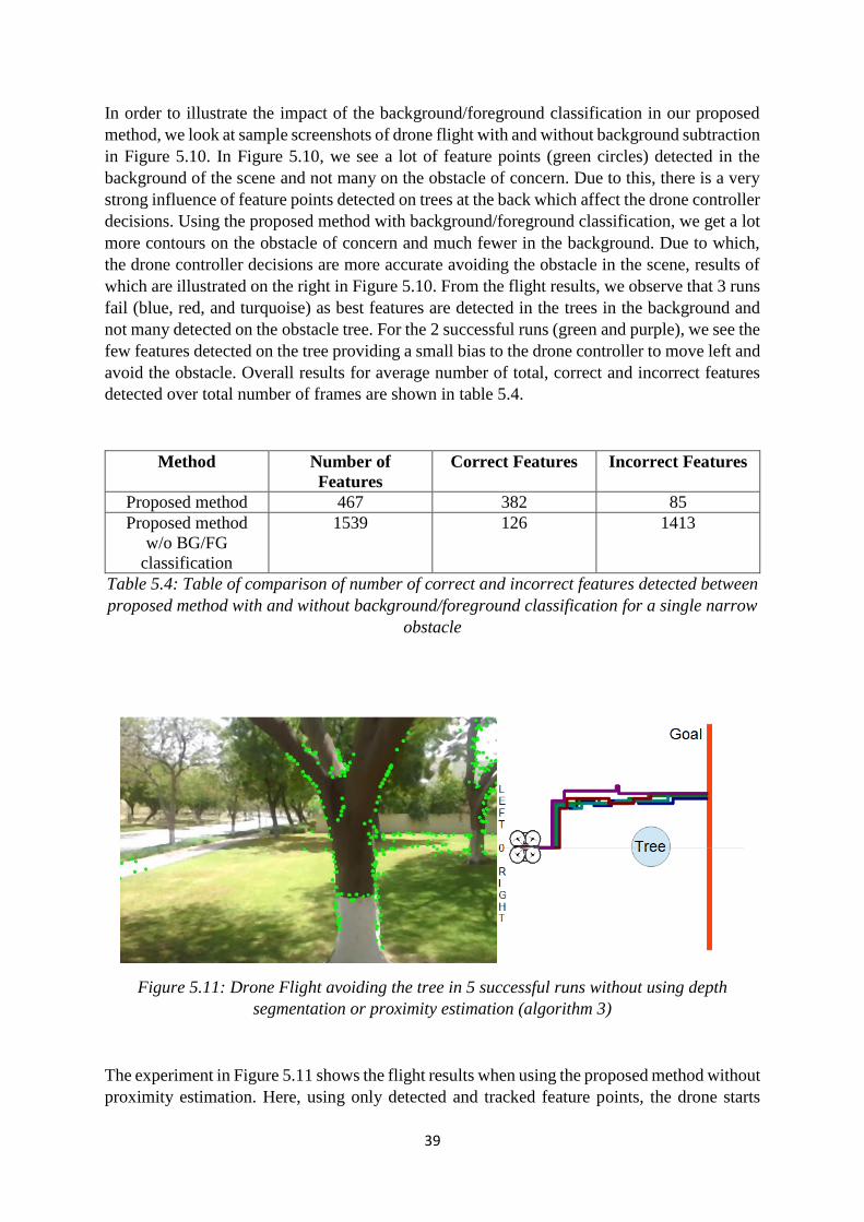
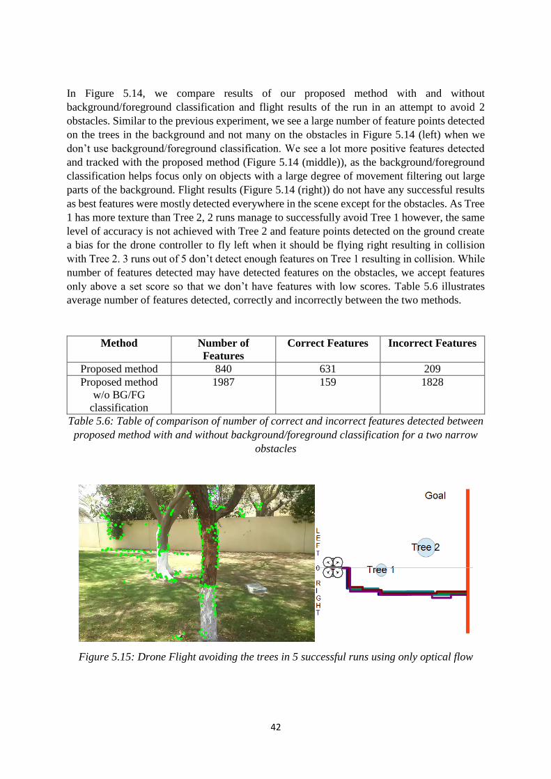
Figure 5.11: Drone Flight avoiding the tree in 5 successful runs without using depth

segmentation or proximity estimation (algorithm 3)

The experiment in Figure 5.11 shows the flight results when using the proposed method without

proximity estimation. Here, using only detected and tracked feature points, the drone starts

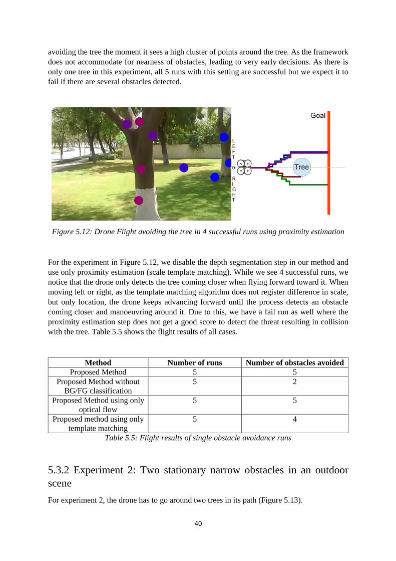
40

avoiding the tree the moment it sees a high cluster of points around the tree. As the framework

does not accommodate for nearness of obstacles, leading to very early decisions. As there is

only one tree in this experiment, all 5 runs with this setting are successful but we expect it to

fail if there are several obstacles detected.

Figure 5.12: Drone Flight avoiding the tree in 4 successful runs using proximity estimation

For the experiment in Figure 5.12, we disable the depth segmentation step in our method and

use only proximity estimation (scale template matching). While we see 4 successful runs, we

notice that the drone only detects the tree coming closer when flying forward toward it. When

moving left or right, as the template matching algorithm does not register difference in scale,

but only location, the drone keeps advancing forward until the process detects an obstacle

coming closer and manoeuvring around it. Due to this, we have a fail run as well where the

proximity estimation step does not get a good score to detect the threat resulting in collision

with the tree. Table 5.5 shows the flight results of all cases.

Method Number of runs Number of obstacles avoided

Proposed Method 5 5

Proposed Method without

BG/FG classification

5 2

Proposed Method using only

optical flow

5 5

Proposed method using only

template matching

5 4

Table 5.5: Flight results of single obstacle avoidance runs

5.3.2 Experiment 2: Two stationary narrow obstacles in an outdoor

scene

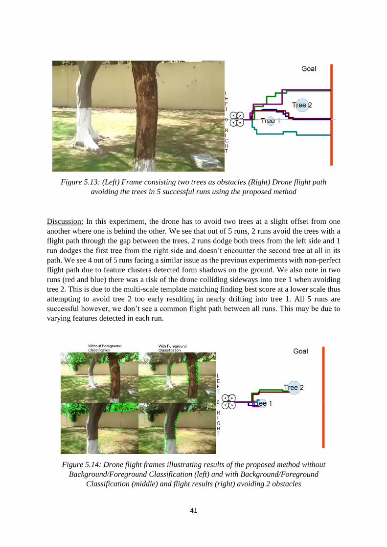
For experiment 2, the drone has to go around two trees in its path (Figure 5.13).

41

Figure 5.13: (Left) Frame consisting two trees as obstacles (Right) Drone flight path

avoiding the trees in 5 successful runs using the proposed method

Discussion: In this experiment, the drone has to avoid two trees at a slight offset from one

another where one is behind the other. We see that out of 5 runs, 2 runs avoid the trees with a

flight path through the gap between the trees, 2 runs dodge both trees from the left side and 1

run dodges the first tree from the right side and doesn’t encounter the second tree at all in its

path. We see 4 out of 5 runs facing a similar issue as the previous experiments with non-perfect

flight path due to feature clusters detected form shadows on the ground. We also note in two

runs (red and blue) there was a risk of the drone colliding sideways into tree 1 when avoiding

tree 2. This is due to the multi-scale template matching finding best score at a lower scale thus

attempting to avoid tree 2 too early resulting in nearly drifting into tree 1. All 5 runs are

successful however, we don’t see a common flight path between all runs. This may be due to

varying features detected in each run.

Figure 5.14: Drone flight frames illustrating results of the proposed method without

Background/Foreground Classification (left) and with Background/Foreground

Classification (middle) and flight results (right) avoiding 2 obstacles

42

In Figure 5.14, we compare results of our proposed method with and without

background/foreground classification and flight results of the run in an attempt to avoid 2

obstacles. Similar to the previous experiment, we see a large number of feature points detected

on the trees in the background and not many on the obstacles in Figure 5.14 (left) when we

don’t use background/foreground classification. We see a lot more positive features detected

and tracked with the proposed method (Figure 5.14 (middle)), as the background/foreground

classification helps focus only on objects with a large degree of movement filtering out large

parts of the background. Flight results (Figure 5.14 (right)) do not have any successful results

as best features were mostly detected everywhere in the scene except for the obstacles. As Tree

1 has more texture than Tree 2, 2 runs manage to successfully avoid Tree 1 however, the same

level of accuracy is not achieved with Tree 2 and feature points detected on the ground create

a bias for the drone controller to fly left when it should be flying right resulting in collision

with Tree 2. 3 runs out of 5 don’t detect enough features on Tree 1 resulting in collision. While

number of features detected may have detected features on the obstacles, we accept features

only above a set score so that we don’t have features with low scores. Table 5.6 illustrates

average number of features detected, correctly and incorrectly between the two methods.

Method Number of

Features

Correct Features Incorrect Features

Proposed method 840 631 209

Proposed method

w/o BG/FG

classification

1987 159 1828

Table 5.6: Table of comparison of number of correct and incorrect features detected between

proposed method with and without background/foreground classification for a two narrow

obstacles

Figure 5.15: Drone Flight avoiding the trees in 5 successful runs using only optical flow

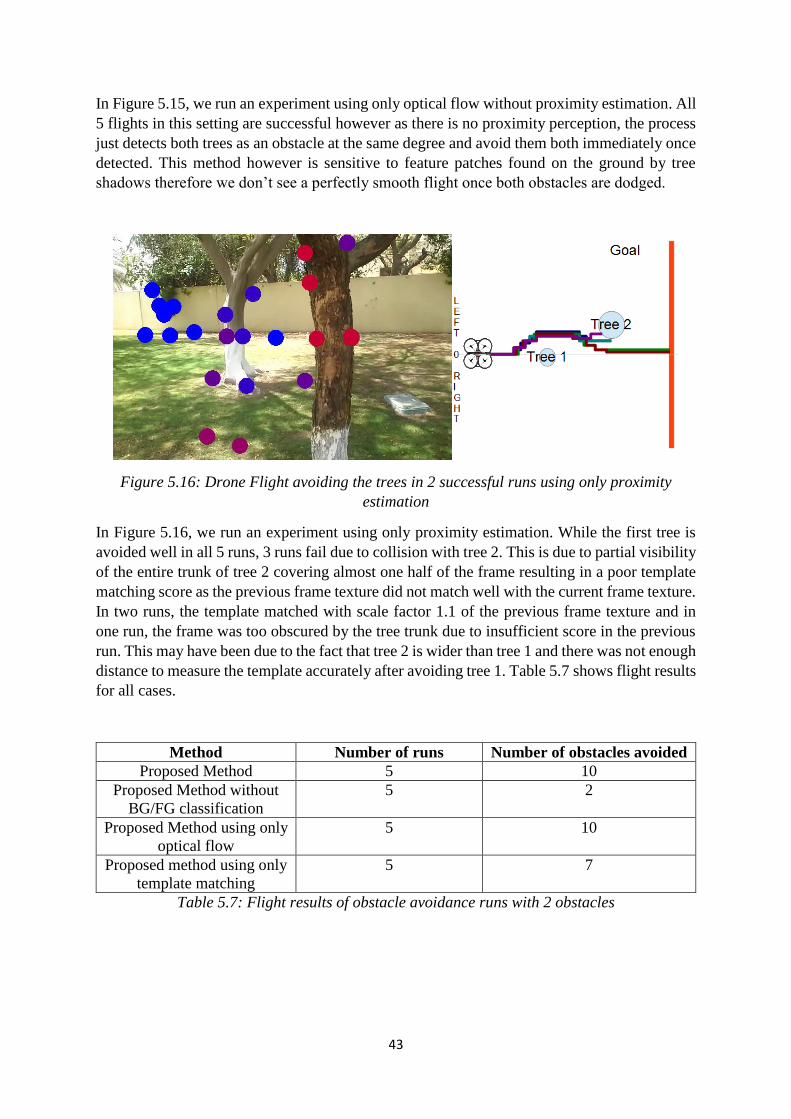
43

In Figure 5.15, we run an experiment using only optical flow without proximity estimation. All

5 flights in this setting are successful however as there is no proximity perception, the process

just detects both trees as an obstacle at the same degree and avoid them both immediately once

detected. This method however is sensitive to feature patches found on the ground by tree

shadows therefore we don’t see a perfectly smooth flight once both obstacles are dodged.

Figure 5.16: Drone Flight avoiding the trees in 2 successful runs using only proximity

estimation

In Figure 5.16, we run an experiment using only proximity estimation. While the first tree is

avoided well in all 5 runs, 3 runs fail due to collision with tree 2. This is due to partial visibility

of the entire trunk of tree 2 covering almost one half of the frame resulting in a poor template

matching score as the previous frame texture did not match well with the current frame texture.

In two runs, the template matched with scale factor 1.1 of the previous frame texture and in

one run, the frame was too obscured by the tree trunk due to insufficient score in the previous

run. This may have been due to the fact that tree 2 is wider than tree 1 and there was not enough

distance to measure the template accurately after avoiding tree 1. Table 5.7 shows flight results

for all cases.

Method Number of runs Number of obstacles avoided

Proposed Method 5 10

Proposed Method without

BG/FG classification

5 2

Proposed Method using only

optical flow

5 10

Proposed method using only

template matching

5 7

Table 5.7: Flight results of obstacle avoidance runs with 2 obstacles

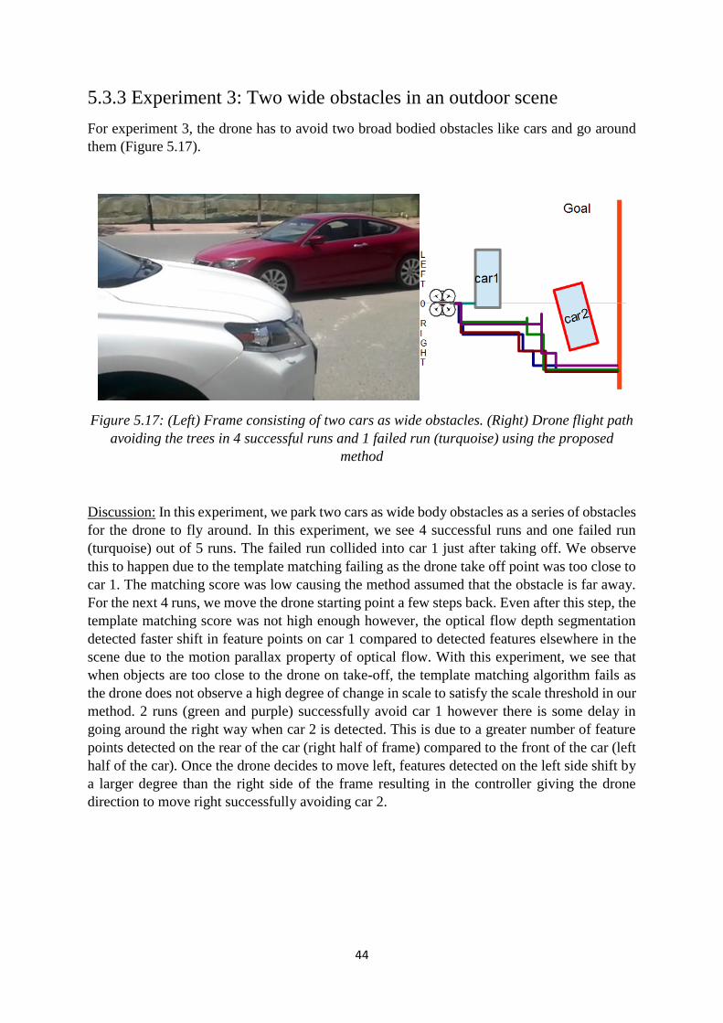
44

5.3.3 Experiment 3: Two wide obstacles in an outdoor scene

For experiment 3, the drone has to avoid two broad bodied obstacles like cars and go around

them (Figure 5.17).

Figure 5.17: (Left) Frame consisting of two cars as wide obstacles. (Right) Drone flight path

avoiding the trees in 4 successful runs and 1 failed run (turquoise) using the proposed

method

Discussion: In this experiment, we park two cars as wide body obstacles as a series of obstacles

for the drone to fly around. In this experiment, we see 4 successful runs and one failed run

(turquoise) out of 5 runs. The failed run collided into car 1 just after taking off. We observe

this to happen due to the template matching failing as the drone take off point was too close to

car 1. The matching score was low causing the method assumed that the obstacle is far away.

For the next 4 runs, we move the drone starting point a few steps back. Even after this step, the

template matching score was not high enough however, the optical flow depth segmentation

detected faster shift in feature points on car 1 compared to detected features elsewhere in the

scene due to the motion parallax property of optical flow. With this experiment, we see that

when objects are too close to the drone on take-off, the template matching algorithm fails as

the drone does not observe a high degree of change in scale to satisfy the scale threshold in our

method. 2 runs (green and purple) successfully avoid car 1 however there is some delay in

going around the right way when car 2 is detected. This is due to a greater number of feature

points detected on the rear of the car (right half of frame) compared to the front of the car (left

half of the car). Once the drone decides to move left, features detected on the left side shift by

a larger degree than the right side of the frame resulting in the controller giving the drone

direction to move right successfully avoiding car 2.

45

Figure 5.18: Drone flight frames illustrating results of the proposed method without

Background/Foreground Classification (left) and with Background/Foreground

Classification (middle) and flight results (right) avoiding 2 wide body obstacles

In Figure 5.18, we see results of the proposed method with and without the

foreground/background classification along with flight results without using the background

subtraction method. In the frames illustrated, we see that there are a lot of features detected

again on background trees and fence in the background of the scene. While there are a few

features detected on the obstacles, most features are detected outside the 2 cars. Due to this,

again we see a strong bias from background objects leading to non-perfect obstacle avoidance

runs. Using the proposed method, a large number of features are detected on the obstacles while

the drone moves closer to the obstacles. When we run flight experiments using the proposed

method but without background/foreground classification, we have two successful runs but 3

unsuccessful runs. When faced with car 1, two runs (red and greed) detect a lot of features on

the tree at the right side of the scene over features detected on the car 1. As not enough features

are detected on car 1, the drone controller did not assume there to be an obstacle ahead resulting

in collision. One run (purple) avoids car 1 and while crossing pass it, large number of incorrect

features in the background and correct features detected on car 2 cause the drone controller to

give instructions to move right colliding into car 1 along the drone’s side. Two successful runs

(blue and turquoise) avoid car 1 and get enough features on car 2 to successfully avoid it as

well despite more features detected on other objects in the scene due to the depth and proximity

estimations employed in the proposed method. Table 5.8 illustrates average number of features

detected, correct and incorrect between the two methods.

Method Number of

Features

Correct Features Incorrect Features

Proposed method 1211 874 337

Proposed method

w/o BG/FG

classification

1384 504 880

Table 5.8: Table of comparison of number of correct and incorrect features detected between

proposed method with and without background/foreground classification for a single narrow

obstacle

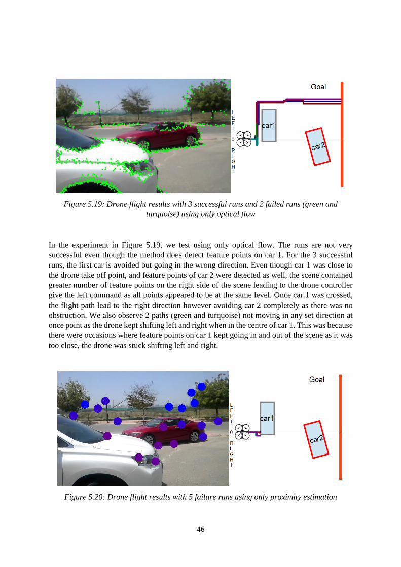
46

Figure 5.19: Drone flight results with 3 successful runs and 2 failed runs (green and

turquoise) using only optical flow

In the experiment in Figure 5.19, we test using only optical flow. The runs are not very

successful even though the method does detect feature points on car 1. For the 3 successful

runs, the first car is avoided but going in the wrong direction. Even though car 1 was close to

the drone take off point, and feature points of car 2 were detected as well, the scene contained

greater number of feature points on the right side of the scene leading to the drone controller

give the left command as all points appeared to be at the same level. Once car 1 was crossed,

the flight path lead to the right direction however avoiding car 2 completely as there was no

obstruction. We also observe 2 paths (green and turquoise) not moving in any set direction at

once point as the drone kept shifting left and right when in the centre of car 1. This was because

there were occasions where feature points on car 1 kept going in and out of the scene as it was

too close, the drone was stuck shifting left and right.

Figure 5.20: Drone flight results with 5 failure runs using only proximity estimation

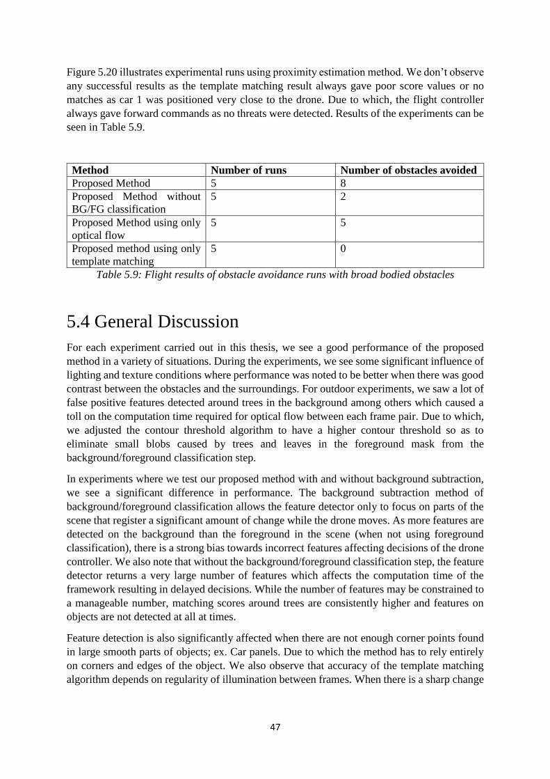
47

Figure 5.20 illustrates experimental runs using proximity estimation method. We don’t observe

any successful results as the template matching result always gave poor score values or no

matches as car 1 was positioned very close to the drone. Due to which, the flight controller

always gave forward commands as no threats were detected. Results of the experiments can be

seen in Table 5.9.

Method Number of runs Number of obstacles avoided

Proposed Method 5 8

Proposed Method without

BG/FG classification

5 2

Proposed Method using only

optical flow

5 5

Proposed method using only

template matching

5 0

Table 5.9: Flight results of obstacle avoidance runs with broad bodied obstacles

5.4 General Discussion

For each experiment carried out in this thesis, we see a good performance of the proposed

method in a variety of situations. During the experiments, we see some significant influence of

lighting and texture conditions where performance was noted to be better when there was good

contrast between the obstacles and the surroundings. For outdoor experiments, we saw a lot of

false positive features detected around trees in the background among others which caused a

toll on the computation time required for optical flow between each frame pair. Due to which,

we adjusted the contour threshold algorithm to have a higher contour threshold so as to

eliminate small blobs caused by trees and leaves in the foreground mask from the

background/foreground classification step.

In experiments where we test our proposed method with and without background subtraction,

we see a significant difference in performance. The background subtraction method of

background/foreground classification allows the feature detector only to focus on parts of the

scene that register a significant amount of change while the drone moves. As more features are

detected on the background than the foreground in the scene (when not using foreground

classification), there is a strong bias towards incorrect features affecting decisions of the drone

controller. We also note that without the background/foreground classification step, the feature

detector returns a very large number of features which affects the computation time of the

framework resulting in delayed decisions. While the number of features may be constrained to

a manageable number, matching scores around trees are consistently higher and features on

objects are not detected at all at times.

Feature detection is also significantly affected when there are not enough corner points found

in large smooth parts of objects; ex. Car panels. Due to which the method has to rely entirely

on corners and edges of the object. We also observe that accuracy of the template matching

algorithm depends on regularity of illumination between frames. When there is a sharp change

48

in illumination, the template matching algorithm returns low scores, and optical flow is also

affected as feature are not matched.

A failed run in experiment 3 shows us that, while the method performs adequately when the

obstacle fits in the frame in its entirety, partially visible obstacles like car 1 with low texture

for a large part of the body cause an impact on the result. We also learn from comparison with

other methods that while optical flow methods work, for obstacles and features moving from

side to side, they don’t function well when faced with walls or very narrow frontal obstacles.

In the case with template matching, we see that it works fairly well when there is adequate

distance between obstacles, but don’t perform too well in tight navigation scenes. The proposed

method having a combination of both methods perform better than them individually but is

subject to scene conditions of illumination and good features to track.

49

6 Conclusion In this thesis, we propose a multi-tiered framework where we employ a number of general

methods in a process flow for the task of obstacle avoidance for aerial drones. Interest in this

area of study have contributed to several approaches to tackle this problem employing a variety

of existing methods and tools to solve this challenge. We take a closer look at methods such as

background/foreground subtraction, feature detection, optical flow, and template matching to

develop a framework that successfully detects, isolates, and avoids obstacles based on

movement, location, and proximity. We look at various enhancements tailored to our case to

the general methods to further improve results.

We then conduct a series of toy and flight experiments in order to infer strengths and

weaknesses of each method and compare it to a collective framework proposed in this study.

We see issues with background subtraction and learn that this method is not enough to keep

track of obstacles when not moving. For this we track moving objects in the foreground result

to follow potential obstacles irrespective of movement by camera or object. We then apply

some heuristics and clustering methods to further refine results of tracking and isolate potential

obstacles from the scene. We then use depth and proximity tools to determine immediate threat

of potential obstacles in the scene and see it perform adequately in a variety of experiments.

We compare results of various combinations of the methods used in the proposed method to

gain insight on the applicability of the method. We see that the proposed method performs

relatively well consistently compared to each method used individually amalgamating to a

more robust framework of methods.

The framework is designed in a way that adding additional modules to it would be simple as

there is one video feed that is used by all modules and each module can run independent of one

another as simple as switching a module on or off. This aspect gives the framework a large

degree of flexibility as it is not constrained to any one type of robot either. To sum the thesis

up, we do see a positive application of the proposed method for applications such as mobile

surveillance, auto-pilot systems, search and rescue missions, traffic management, military

applications as well as domestic applications.

50

7 Future Work

With some additional or improved methods to segment obstacles based on edges and colour

information, the framework is guaranteed to perform even better. Below we outline some

possible future work on this research for improvement:

Segmentation based on colour and adding that information to the confidence image

A drone with faster data transmission speed would help the video feed input stream

and quick navigation decisions may be made

Processing frames on a newer and faster CPU to improve post-processing frame rate

Adding a learning method to detect known obstacles faster by using trained classifiers

Using a combination of colour as well as edge/corner features for tracking

Using another tracking method than optical flow once an object is successfully

segmented

Adding a TLD-like method for tracking, learning and detection12 of obstacles

Additional hardware such as range-finders would definitely improve confidence

results

Pre-existing knowledge of environment would help the accuracy of detection

significantly

A variety of extensions to the proposed method are possible and not limited by applicability

in any scenario.

12 http://personal.ee.surrey.ac.uk/Personal/Z.Kalal/tld.html

51

8 References

[1] Zhou W., Liu y., Zhuang L., Yu N., “Dynamic Background Subtraction using Spatial-Color

Binary Patters”. University of Science and Technology of China, 2011 Sixth International

Conference on Image and Graphics

[2] Barnich O., Van Droogenbroeck M., “ViBe: A Universal Background Subtraction

Algorithm for Video Sequences”. IEEE Transactions on Image Processing, Vol. 20, No. 6,

June 2011

[3] Sheikh y., Javed O., Kanade T., “Background Subtraction for Freely Moving Cameras”.

Carnegie Mellon University.

[4] KaewTraKulPong P., Bowden R., “An Improved Adaptive Background Mixture Model for

Real-Time Tracking with Shadow Detection”. 2nd European Workshop on Advanced Video

Based Surveillance Systems, AVBS01, September 2011.

[5] Reddy V., Sanderson C., Lovell B.C., “Improved Foreground Detection via Block-Based

Classifier Cascade with Probabilistic Decision Integration”. The University of Queensland.

[6] Mountney P., Stoyanov D. and Yang G. (2010), "Three-Dimensional Tissue Deformation

Recovery and Tracking: Introducing techniques based on laparoscopic or endoscopic images."

IEEE Signal Processing Magazine. 2010 July. Volume: 27". IEEE Signal Processing Magazine

27 (4): 14–24. doi:10.1109/MSP.2010.936728.

[7] Mihaylova L., Brasnett P., Canagarajan N. and Bull D.(2007), Object Tracking by Particle

Filtering Techniques in Video Sequences; In: Advances and Challenges in Multisensor Data

and Information. NATO Security through Science Series, 8. Netherlands: IOS Press. pp. 260–

268. ISBN 978-1-58603-727-7.

[8] Comaniciu, D.; Ramesh, V.; Meer, P., "Real-time tracking of non-rigid objects using mean

shift," Computer Vision and Pattern Recognition, 2000. Proceedings. IEEE Conference on,

vol.2, no., pp.142, 149 vol.2, 2000

52

[9] Yilmaz A., Javed O., Shar M., “Object Tracking: A Survey”. ACM Computing Surveys,

Vol. 38, No. 4, Article 13, December 2006.

[10] M. Arulampalam, S. Maskell, N. Gordon, and T. Clapp (2002). "A Tutorial on Particle

Filters for Online Nonlinear/Non-Gaussian Bayesian Tracking". IEEE Trans. on Signal

Processing 50 (2): 174.

[11] B. D. Lucas and T. Kanade (1981), “An iterative image registration technique with an

application to stereo vision.” Proceedings of Imaging Understanding Workshop, pages 121—

130

[12] C. Harris and M. Stephens (1988). "A combined corner and edge detector". Proceedings

of the 4th Alvey Vision Conference. pp. 147–151.

[13] J. Shi and C. Tomasi (June 1994). "Good Features to Track,” 9th IEEE Conference on

Computer Vision and Pattern Recognition. Springer.

[14] C. Tomasi and T. Kanade (2004). "Detection and Tracking of Point Features". Pattern

Recognition37: 165–168.

[15] H. Wang and M. Brady (1995). "Real-time corner detection algorithm for motion

estimation".Image and Vision Computing 13 (9): 695–703.

[16] Kim J., Do Y., “Moving obstacle avoidance of a mobile robot using a single camera”.

International Symposium on Robotics and Intelligent Sensors 2012 (IRIS 2012)

[17] Kundu A., Jawahar C.V., Krishna M., “Realtime Moving Object Detection from a Freely

Moving Monocular Camera”. International Conference on Robotics and Biometrics, December

2010

[18] Nishigaki M., Aloimonos Y., “Moving Obstacle Detection using Cameras for Driver

Assistance System”. IEEE Intelligent Vehicles Symposium 2010

[19] De Croon G.C.H.E., deWeerdt E., de Wagter C., Remes B.D.W., “The appearance

variation cue for obstacle avoidance”. IEEE International Conference on Robotics and

Biomimetics 2010.

53

[20] Goroshin R., “Obstacle Detection Using a Monocular Camera”. Master Thesis, Georgia

Institute of Technology, August 2008.

[21] Liem M., Visser A., Groen F., “A Hybrid Algorithm for Tracking and Following People

using a Robotic Dog”. University of Amsterdam.

[22] S. Kang, J. Paik, A. Koschan, B. Abidi, and M. A. Abidi (2003). "Real-time video tracking

using PTZ cameras". Proc. Of SPIE 5132: 103–111.

[23] Black, James, Tim Ellis, and Paul Rosin (2003). "A Novel Method for Video Tracking

Performance Evaluation". Joint IEEE Int. Workshop on Visual Surveillance and Performance

Evaluation of Tracking and Surveillance: 125–132.

[24] Mori T., Scherer S., “First Results in Detecting and Avoiding Frontal Obstacles from a

Monocular Camera for Micro Unmanned Aerial Vehicles”. IEEE Internation Conference on

Robotics and Automation 2013 (ICRA).

[25] Yankun Z., Chuyang H., Weyrich, Norman, “A Single Camera Based Rear Obstacle

Detection System”. IEEE Intelligent Vehicles Symposium, June 2011.

[26] Reina, G., Vargas, A., Keiji Nagatani,, Kazuya Yoshida, “Adaptive Kalman Filtering for

GPS-based Mobile Robot Localization”. Safety, Security and Rescue Robotics, 2007. SSRR

2007. IEEE International Workshop.

[27] N. Dijkshoorn (2012), “Simultaneous Localization and Mapping with the AR. Drone”.

Master Thesis, University of Amsterdam.

[28] Ioannis M. Rekleitis. "A Particle Filter Tutorial for Mobile Robot Localization." Centre

for Intelligent Machines, McGill University, Tech. Rep. TR-CIM-04-02 (2004).

[29] Lu X., Manduchi R., “Fast image motion segmentation for surveillance applications”.

University of California, Image and Vision Computing 29 (2011).

54

[30] Narkhede H.P., “Review of Image Segmentation Techniques”. International Journal of

Science and Modern Engineering. ISSN: 2319-6386, Volume-1, Issue-8, July 2013

[31] Karasulu B. (2010), “Review and Evaluation of Well-Known Methods for Moving Object

Detection and Tracking in Videos”. Ege University, Turkey.

[32] B. Tamersoy (September 29, 2009)."Background Subtraction – Lecture Notes". University

of Texas at Austin

[33] Y. Benezeth; B. Emile; H. Laurent; C. Rosenberger (December 2008). "Review and

evaluation of commonly-implemented background subtraction algorithms". 19th International

Conference on Pattern Recognition. pp. 1–4.

[34] C.R. Wren; A. Azarbayejani; T. Darrell; A.P. Pentland (July 1997). "Pfinder: real-time

tracking of the human body". IEEE Transactions on Pattern Analysis and Machine Intelligence

19 (7): 780–785.

[35] C. Stauffer, W. E. L. Grimson (August 1999). "Adaptive background mixture models for

real-time tracking". IEEE Computer Society Conference on Computer Vision and Pattern

Recognition 2. pp. 246–252

[36] T. Bouwmans; F. El Baf; B. Vachon (November 2008). "Background Modeling using

Mixture of Gaussians for Foreground Detection - A Survey". Recent Patents on Computer

Science 1: 219–237.

[37] Stauffer C, Grimson W. E. L. Adaptive background mixture models for real-time tracking.

in Proceedings. 1999 IEEE Computer Society Conference on Computer Vision and Pattern

Recognition (Cat. No PR00149). IEEE Comput. Soc. Part Vol. 2, 1999.

[38] Stauffer C, Grimson W. E. L., Learning patterns of activity using real-time tracking. IEEE

Transactions on Pattern Analysis & Machine Intelligence, 2000. 22(8): p. 747-57.

[39] Jean-Yves Bouguet, “Pyramidal Implementation of the Lucas Kanade Feature Tracker

Description of the algorithm”, Intel Corporation Microprocessor Research Labs.

55

[40] A. Beyeler, J. Zufferey, and D. Floreano, “3D Vision-based Navigation for Indoor

Microflyers,” Proceedings IEEE International Conference on Robotics and Automation, 2007.

[41] P. Oh, W. Green, and G. Barrows, “Neural nets and optic flow for autonomous micro-air-

vehicle navigation,” Proc. Int. Mech. Eng. Congress and Exposition, 2004.

[42] W. Green and P. Oh, “Optic-Flow-Based Collision Avoidance,” Robotics & Automation

Magazine, IEEE, 2008.

[43] P. C. Merrell, D.-J. Lee, and R.W. Beard, “Obstacle Avoidance for Un-manned Air

Vehicles Using Optical Flow Probability Distributions,” Mobile Robots XVII, 2004.

[44] C. Bills, J. Chen, and A. Saxena, “Autonomous MAV flight in indoor environments using

single image perspective cues,” in Robotics and Automation (ICRA), 2011 IEEE International

Conference on, 2011.

[45] K. Celik, S.-J. Chung, M. Clausman, and A. Somani, “Monocular vision SLAM for indoor

aerial vehicles,” Intelligent Robots and Systems, 2009. IROS 2009. IEEE/RSJ International

Conference on, 2009

[46] J.-O. Lee, K.-H. Lee, S.-H. Park, S.-G. Im, and J. Park, “Obstacle avoidance for small

UAVs using monocular vision,” Aircraft Engineering and Aerospace Technology, 2011.

[47] J. Michels, A. Saxena, and A. Ng, “High speed obstacle avoidance using monocular vision

and reinforcement learning,” ICML ’05: Proceedings of the 22nd international conference on

Machine learning, 2005.

[48] D. N. Lee, “A theory of visual control of braking based on information about time-to-

collision,” Perception, 1976

[49] M. J. Brooks, W. Chojnacki, and L. Baumela. Determining the egomotion of an

uncalibrated camera from instantaneous optical flow. Journal of the Optical Society of America

A, 1997.

[50] B. Kelly. Structure from stereo vision using optical flow. Master’s thesis, University of

Canterbury, November 2006.

[51] T. Low and G. Wyeth. Learning to avoid indoor obstacles from optical flow, December

2007.

[52] Murtagh, Fionn (1983), "A survey of recent advances in hierarchical clustering

algorithms", The Computer Journal 26 (4): 354–359.

[53] R. Brunelli, “Template Matching Techniques in Computer Vision: Theory and Practice”.

ISBN: 987-0-470-51706-2. March 2009.