of analysing document similarity measures
TRANSCRIPT

University of OxfordComputing Laboratory
MSc Computer ScienceDissertation
Analysing Document SimilarityMeasures
Author:Edward Grefenstette
Supervisor:Professor Stephen Pulman
November 10, 2010

2

Abstract
The concept of a Document Similarity Measure is ill-defined due to the widevariety of existing metrics measuring a range of often very different notionsof similarity. The crucial role of measuring document similarity in a widevariety of text and language processing tasks calls not only for a betterunderstanding of how metrics work in general terms, but also a better wayof analysing, comparing and improving document similarity measures.
This dissertation supplies an overview of different theoretical positions on thenotion of similarity, discusses the construction of a framework for analysingand comparing a wide variety of metrics against a testbed corpus subdi-vided into categories by similarity type, and finally presents the results of anexperiment run using this framework.
We found that the metric rankings and breakdown of results justified thetheoretical position we developed while considering the nature of similarity,and that there is no deep distinction between syntactic, lexical and semanticsimilarity features. The results of our experiments also allowed us to positvarious methods for developing better document similarity measures, usingthe output of the analysis framework to motivate their construction.
3

4

Contents
Abstract 3
List of Figures 9
List of Tables 11
Acknowledgements 13
1 Introduction 15
2 Background and Theory 192.1 Philosophical Foundations . . . . . . . . . . . . . . . . . . . . 19
2.1.1 Platonist Similarity . . . . . . . . . . . . . . . . . . . . 202.1.2 Similarity and the Foundation of Mathematics . . . . . 202.1.3 Davidson on Similarity in Metaphors . . . . . . . . . . 212.1.4 Similarity in the Cognitive Sciences . . . . . . . . . . . 222.1.5 Wittgenstein on Similarity . . . . . . . . . . . . . . . . 23
2.2 Different kinds of Document Similarity . . . . . . . . . . . . . 252.2.1 Three Classes of Document Similarity . . . . . . . . . . 252.2.2 Similarity Features . . . . . . . . . . . . . . . . . . . . 262.2.3 Cross-Category Similarity Features . . . . . . . . . . . 272.2.4 Classifying Similarity Types . . . . . . . . . . . . . . . 28
2.3 Dropping the Class Distinction . . . . . . . . . . . . . . . . . 30
3 Methodology 333.1 Constructing a Corpus . . . . . . . . . . . . . . . . . . . . . . 34
3.1.1 Selecting Document Similarity Types . . . . . . . . . . 343.1.2 Designing a Corpus Construction Framework . . . . . . 37
5

6 CONTENTS
3.1.3 Setting the Gold-Standard . . . . . . . . . . . . . . . . 383.1.4 Mixing Things Up (If Needed) . . . . . . . . . . . . . . 39
3.2 Evaluating Metrics: Considerations and Concerns . . . . . . . 413.2.1 Dealing with the Corpus . . . . . . . . . . . . . . . . . 423.2.2 Normalising the Results . . . . . . . . . . . . . . . . . 433.2.3 Adapting Word/Character-based Metrics . . . . . . . . 43
3.3 Analysis: The Devil in the Details . . . . . . . . . . . . . . . . 443.3.1 Gold-Standard Ranking vs. Retrieval . . . . . . . . . . 453.3.2 Finer-grain Analysis: Breaking Down Results . . . . . 47
4 Designing a Corpus Construction Module 514.1 Setting Up a General Framework . . . . . . . . . . . . . . . . 51
4.1.1 Structure and Shared Features . . . . . . . . . . . . . . 514.1.2 Suggested Improvements . . . . . . . . . . . . . . . . . 55
4.2 Syntactic Toy-Corpora . . . . . . . . . . . . . . . . . . . . . . 554.2.1 General Overview . . . . . . . . . . . . . . . . . . . . . 554.2.2 Construction Process: Random Edits Corpus . . . . . . 564.2.3 Construction Process: POS-Tag Equivalence Corpus . . 59
4.3 Theme-grouped Texts . . . . . . . . . . . . . . . . . . . . . . . 614.3.1 General Overview . . . . . . . . . . . . . . . . . . . . . 614.3.2 Construction Process . . . . . . . . . . . . . . . . . . . 61
4.4 Wikipedia Article Pairs . . . . . . . . . . . . . . . . . . . . . . 634.4.1 General Overview . . . . . . . . . . . . . . . . . . . . . 634.4.2 Background and Sources . . . . . . . . . . . . . . . . . 634.4.3 Construction Process . . . . . . . . . . . . . . . . . . . 644.4.4 Future Improvements . . . . . . . . . . . . . . . . . . . 65
4.5 Paraphrase Corpora . . . . . . . . . . . . . . . . . . . . . . . . 664.5.1 General Overview . . . . . . . . . . . . . . . . . . . . . 664.5.2 Background and Sources . . . . . . . . . . . . . . . . . 664.5.3 Construction Process . . . . . . . . . . . . . . . . . . . 674.5.4 Future Improvements . . . . . . . . . . . . . . . . . . . 70
4.6 Abstract-Paper Pairs . . . . . . . . . . . . . . . . . . . . . . . 704.6.1 General Overview . . . . . . . . . . . . . . . . . . . . . 704.6.2 Background and Sources . . . . . . . . . . . . . . . . . 714.6.3 Construction Process . . . . . . . . . . . . . . . . . . . 714.6.4 Future Improvements . . . . . . . . . . . . . . . . . . . 72
5 Evaluating Document Similarity Measures 75

CONTENTS 7
5.1 Generalised Evaluation Framework . . . . . . . . . . . . . . . 765.2 Implementing Purely Syntactic Metrics . . . . . . . . . . . . . 77
5.2.1 Character-Count and Word-Count . . . . . . . . . . . . 785.2.2 Levenshtein Edit Distance . . . . . . . . . . . . . . . . 785.2.3 Jaro-Winkler Distance . . . . . . . . . . . . . . . . . . 795.2.4 Ratio Similarity . . . . . . . . . . . . . . . . . . . . . . 805.2.5 Jaccard Similarity . . . . . . . . . . . . . . . . . . . . . 805.2.6 MASI Distance . . . . . . . . . . . . . . . . . . . . . . 81
5.3 BLEU: A Machine Translation Evaluation Metric . . . . . . . 825.3.1 Origin and use . . . . . . . . . . . . . . . . . . . . . . 825.3.2 Implementation and score normalisation . . . . . . . . 83
5.4 Wordnet-based Metrics . . . . . . . . . . . . . . . . . . . . . . 835.4.1 Overview of Wordnet Metrics . . . . . . . . . . . . . . 845.4.2 Implementing Wordnet-based Metrics . . . . . . . . . . 865.4.3 Fine-tuning: How Far is Too Far? . . . . . . . . . . . . 87
5.5 Semantic Vectors . . . . . . . . . . . . . . . . . . . . . . . . . 885.5.1 Background Theory . . . . . . . . . . . . . . . . . . . . 895.5.2 Implementation: A Different Approach to Word-Sentence
Scaling . . . . . . . . . . . . . . . . . . . . . . . . . . . 90
6 Results and Analysis 936.1 Structure of Analysis Script . . . . . . . . . . . . . . . . . . . 936.2 Discussion of Metric CGS Scores . . . . . . . . . . . . . . . . 95
6.2.1 Overall Rankings . . . . . . . . . . . . . . . . . . . . . 956.2.2 Random Edits Analysis . . . . . . . . . . . . . . . . . . 966.2.3 POS-Switch Analysis . . . . . . . . . . . . . . . . . . . 1006.2.4 Theme Analysis . . . . . . . . . . . . . . . . . . . . . . 1016.2.5 Wikipedia Analysis . . . . . . . . . . . . . . . . . . . . 1026.2.6 Paraphrase Analysis . . . . . . . . . . . . . . . . . . . 1036.2.7 Abstract-Article Analysis . . . . . . . . . . . . . . . . . 104
7 Conclusions 119
Bibliography 123
A Technical Details 127A.1 Supplied CD-ROM Contents . . . . . . . . . . . . . . . . . . . 127A.2 System Requirements . . . . . . . . . . . . . . . . . . . . . . . 130

8 CONTENTS
B Source Code 131B.1 corpusbuilder.py . . . . . . . . . . . . . . . . . . . . . . . . . . 131B.2 buildcorpus.py . . . . . . . . . . . . . . . . . . . . . . . . . . . 140B.3 prepcorpus.py . . . . . . . . . . . . . . . . . . . . . . . . . . . 143B.4 corpusevaluation.py . . . . . . . . . . . . . . . . . . . . . . . . 145B.5 semanticvectors.java . . . . . . . . . . . . . . . . . . . . . . . 152B.6 evaluatecorpus.py . . . . . . . . . . . . . . . . . . . . . . . . . 155B.7 analyser.py . . . . . . . . . . . . . . . . . . . . . . . . . . . . 157

List of Figures
2.1 Classes, Properties and Types of Document Similarity . . . . . 26
3.1 Example of Visually Represented CGS Score Distribution . . . 47
6.1 Levenshtein Edit Distance CGS Score Distribution (Edits Sec-tion) . . . . . . . . . . . . . . . . . . . . . . . . . . . . . . . . 98
6.2 Jaro-Winkler Distance CGS Score Distribution (Edits Section) 996.3 Comparison of BLEU and Path Similarity for POS-switch Docs1076.4 Comparison of BLEU and Path Similarity for Matched POS-
switch Docs . . . . . . . . . . . . . . . . . . . . . . . . . . . . 1086.5 Comparison of BLEU and Path Similarity for Mixed POS-
switch Docs . . . . . . . . . . . . . . . . . . . . . . . . . . . . 1096.6 Comparison of Character Count and MASI for Theme Docu-
ments . . . . . . . . . . . . . . . . . . . . . . . . . . . . . . . 1106.7 Breakdown of Semantic Vectors CGS Distribution for Wikipedia
Docs . . . . . . . . . . . . . . . . . . . . . . . . . . . . . . . . 1116.8 Comparison of Semantic Vectors and Path Sim. for Para-
phrase Docs . . . . . . . . . . . . . . . . . . . . . . . . . . . . 1126.9 Comparison of Semantic Vectors and Path Sim. for Matched
Paraphrase Docs . . . . . . . . . . . . . . . . . . . . . . . . . 1136.10 Comparison of Semantic Vectors and Path Sim. for Mixed
Paraphrase Docs . . . . . . . . . . . . . . . . . . . . . . . . . 1146.11 Comparison of Jaccard and MASI Distances for Paraphrase
Docs . . . . . . . . . . . . . . . . . . . . . . . . . . . . . . . . 1156.12 Comparison of Jaccard and MASI Distances for Matched Para-
phrase Docs . . . . . . . . . . . . . . . . . . . . . . . . . . . . 1166.13 Comparison of Jaccard and MASI Distances for Mixed Para-
phrase Docs . . . . . . . . . . . . . . . . . . . . . . . . . . . . 117
9

10 LIST OF FIGURES
6.14 Semantic Vectors CGS Score Distribution (Abstracts) . . . . . 118

List of Tables
6.1 Corpus Category Legend . . . . . . . . . . . . . . . . . . . . . 966.2 Overall Rankings (% CGS Scores) . . . . . . . . . . . . . . . . 976.3 Matched Document Pair Rankings (% CGS Scores) . . . . . . 976.4 Mixed Document Pair Rankings (% CGS Scores) . . . . . . . 106
11

12 LIST OF TABLES
Acknolwedgements
First and foremost, thanks to Stephen Pulman for his supervision and hissupport throughout this project for which he proposed the subject matterin the first place. His constant feedback and bibliographical pointers werealways helpful, and this work would not have been of the same quality if hehad not taken time out of his packed head-of-department schedule to arrangeregular supervision meetings.
Much gratefulness is due to Edward Loper and Stephen Bird, not only for de-veloping the Natural Language Processing Toolkit and writing an amazinglyclear companion book, but also for taking the time to answer my many ques-tions about both the toolkit’s technical hitches and how to approach specificissues of metric evaluation, which came in handy while thinking about howto deal with word-based Wordnet metrics.
Thanks also to Pascal Combescot for his helpful suggestions in the earlystages of this project, and for sharing his implementation of Dominic Wid-dows’ excellent Semantic Vectors package; to Simon Zwarts for his C imple-mentation of the BLEU metric; to the anonymous coders behind the PopplerPDF tools and those behind the Levenshtein metric package; and to SeanHeelan for (unsuccessfully) helping me troubleshoot my installation of theMETEOR metric for evaluating machine translation, which didn’t make thecut. We tried.
Finally, thanks to my parents Irene and Greg Grefenstette, as well as mygrandparents for their support of various sorts over the years, without whichI wouldn’t have had the peace of mind to finish large projects like this oneon time.
13

14 LIST OF TABLES
Edward T. Grefenstette

Chapter 1
Introduction
Evaluating the similarity between two documents is an operation which liesat the heart of most text and language processing tasks. Once we con-sider ‘document’ to mean not a file or placeholder for information contentas dictated by the everyday use of the term, but rather a delineable unitof information (be it a paragraph, an article, a sentence or even a word, inthe case of textually represented information), then the fact that evaluat-ing document similarity is an essential operation to such tasks should be-come intuitively clear by examination of a few common examples of text orlanguage-processing tasks. We give systems which perform such evaluationsthe name of document similarity measures (DSMs) or document similaritymetrics1.
To give a few examples: when we make use of a search engine, we requestweb-page documents which bear some similarity to the keywords or string(s)which constitute the query document; when we ask for a text in some lan-guage A to be translated into some language B, we request a document inlanguage B which has some similarity to the document in language A; whenwe summarise one document, we seek to produce another document which issimilar in some ways (e.g. core meaning being preserved), which however isalso different in other ways (the summary must be shorter than the originaldocument, sentences are more compact). Naturally, such use of documentsimilarity could easily involve other media than text, such as pictures, film,
1Both terms are generally used interchangeably in the literature, and will be used sohere.
15
16 CHAPTER 1. INTRODUCTION
audio, etc. However, the metrics for such media can understandably be verydifferent (and often more primitive) from the ones we will be consideringin text processing, and therefore we will consider non-text documents to beoutside of the scope of this discussion.
The above few examples illustrate an interesting point, which would beequally observed in any further examples of document similarity use: al-though the abstract task being completed in each example—that of attempt-ing to compute some sort of similarity between sets of documents in orderto achieve some practical goal (classification, validation, generation, etc.)—isthe same in each case, the notion of similarity at play is not. Indeed, thesimilarity we draw upon when ranking documents according to word-countis much different than that which we use when translating sentences, whichitself is very different from that which we use when summarising text. Inthe word-count case, we care only about superficial syntactic features; inthe translation case, perhaps we look for shared lexical features, and in thesummarisation case we not only draw upon semantic features, but also uponsyntactic features similar to those exploited in the word-count case (since wewant a shorter summary document).
The observation that DSMs are systems that perform the same abstract taskwhile drawing upon very different aspects of documents depending on thecomparison goals raises a few questions about the nature of DSMs. What isthe common thread to DSM design? Is it a software engineering problem,or are there general principles underlying their construction? Are metricsdesigned for one purpose suitable for another? How would we determinethis if they were? How do DSMs deal with different kinds of input (words,sentences, sets of paragraphs)? On what grounds can we compare metrics?How do we choose a ‘better’ metric relative to a task?
This jumble of questions justifies further investigation, but leaves us withlittle clue as to how to begin. Attempts have been made in the computationallinguistics literature to answer some of these questions with regard to smallgroups of metrics, particularly within the context of comparing two specifictypes of metrics (e.g. see (Agirre et al. 2009)), however we found no attemptat giving a general theory of DSM design and analysis in the literature, andhave resolved to approach the problem ourselves.
The common theme to the above questions can be synthesised into the fol-lowing three key questions which will form the basis of our investigation.
17
Firstly, how are common DSMs designed and implemented? We wish, inanswering this question, to learn more about the kinds of metrics commonlyused in text processing, and the sort of difficulties arising when consideringhow to use them in practice. Secondly, how can we analyse DSMs? In an-swering this question—which will form the bulk of our project—we wish todiscover how DSMs can be compared and ranked relative to different types ofdocument similarity, thus giving us some insight into their performance fora variety of text processing tasks. Thirdly and finally, how can the resultsof such analysis be leveraged to improve existing DSMs or produce betterDSMs?
In order to answer these questions, we designed and implemented a tripartiteDSM evaluation system structured as follows: we first constructed a systemcapable of generating and annotating a structured corpus composed of pairsof documents categorised by the type of similarity associating them, in ad-dition to a gold-standard similarity score; we then built a framework whichuses the aforementioned corpus as a testbed for evaluating a variety of DSMsby checking the metric score for each document pair in the corpus against thegold-standard similarity score; and finally we wrote an analysis frameworkwhich breaks down the results of the evaluation and produces finer anal-ysis of the results, allowing for a better understanding of different DSM’sperformances for different similarity types, as well as clearer inter-metriccomparison.
The subsidiary goals of this project were therefore to produce an extensibleframework for evaluating, comparing and analysing metrics, in addition toour main goal of producing results which might allow us to answer the threemain questions discussed above. To present how we have attempted to reachthese goals, we have structured this dissertation as follows: in Chapter 2we will briefly present some of the linguistic and philosophical backgroundto the definition of similarity in order to clarify the concepts we will bedealing with throughout this work; in Chapter 3, we will present the conceptof the tripartite framework we constructed in more detail and discuss someissues we considered before beginning the design process; in Chapter 4 we willpresent the structure of the corpus generation framework, and discuss specificissues with designing the corpus categories we used in our final experimentalanalysis; in Chapter 5 we will discuss the general structure of DSM evaluationframework, as well as discuss the difficulties faced while implementing thespecific metrics used in our experiment (particularly the semantic similarity

18 CHAPTER 1. INTRODUCTION
metrics, discussed in §§5.4–5.5); and in Chapter 6 we will discuss the designof our evaluation framework, but also present and comment upon the resultsof our experiment, wherein we aim to discover how well individual DSMsperform for the corpus section corresponding to the sort of similarity theywere designed to measure, and whether there are any ‘surprises’—i.e. DSMswhich perform well for similarity types they were not originally designed todeal with. Finally, in the conclusion—Chapter 7—we will review the resultsof previous chapters, see how far we have come towards reaching the goals andanswering the questions set out in the present chapter, and discuss how theresults of analysis could be used to improve existing metrics and/or designnew metrics capable of dealing with complex kinds of similarity (typicallysorts of semantic similarity) in future work.
Additionally, although we will discuss some potential further work in ourconclusion, because our project revolved around constructing an extensibleframework for the construction of a testbed corpus and the evaluation andanalysis of DSMs, we will mostly be synthesising the suggestions for futurework and further improvements which we will be making throughout this dis-sertation. The general purpose of this project is thus not just to learn aboutDSMs and how to improve them, but to condone (and hopefully exemplify)a more rigorous, scientific approach to text processing and computationallinguistics as a whole.

Chapter 2
Background and Theory
In this chapter, we wish to clarify the core concepts we will be discussingthroughout the dissertation (cf. §2.1), in particular that of what ‘similar-ity’ could be taken to mean in the context of ‘document similarity’. Usingsuch definitions as a basis, we will attempt to clarify what different kindsof document similarity there might be (cf. §2.2). Discussion of the theo-retical background for individual DSMs, which one might expect to find inthis chapter, will instead be provided when discussing individual metrics inChapter 5. Finally we will attempt to draw conclusions relating the resultsof the discussion in this chapter to the structure and goals of this project in§2.3.
2.1 Philosophical Foundations
The definition of ‘similarity’ in the philosophical domain seems as nebu-lous as the domain itself. Indeed, the absence of a definition for the termin the otherwise-well-rounded Oxford Dictionary of Philosophy (Blackburn1996) may serve as an indication that the term lacks a definite description.However, a broad notion of similarity exists in the philosophical literaturesince Hellenic times, usually implicitly understood as the fidelity of property-conservation between an object and its reference. However, this broad defi-nition does not always fully fit the notion of similarity involved in DSMs, aswe shall see below.
19

20 CHAPTER 2. BACKGROUND AND THEORY
2.1.1 Platonist Similarity
For instance, in Plato’s Republic (cf. Griffith and Ferrari (2000), booksVI–VII), it is discussed how what defines a class of objects is the sharingof features of ideal objects. For instance, a chair is similar to another chairbecause they both have properties relating them to an ideal chair which Platocalls the (conceptual) form of a chair (e.g. back and seat, one or more legselevating it from ground level, etc.), even though they may differ with regardto other properties (e.g. colour, construction material, presence of arm-rests,etc.).
Judging the similarity of entities by examining their sharing of an ideal formmay seem intuitive enough, but there are several problems. First, it seems wemust commit ourselves to the possibility of abstract/general enough formsfor non-trivial comparisons to be made: to illustrate, a stool and a chair areintuitively similar, but if we do not commit to their being a hierarchy of formsin which some ideal amalgamate of the forms of chairs and stools exists, wecannot evaluate their similarity under a such platonist-inspired system.
However, if we do allow for such a hierarchy, we must not only specify howdegree of similarity is to be judged, but more importantly we must also de-scribe limiting conditions for the stipulation of such amalgamations of forms,lest we allow for any two objects to be qualified as similar through the pos-tulation that there exists some ideal amalgamation of their correspondingforms (for example we might say that a chair and a whale are similar be-cause both have essential properties of the ideal form of things that existphysically). This objection, it turns out, is fairly similar one presented byDavidson, which we will discuss below.
2.1.2 Similarity and the Foundation of Mathematics
Later metaphysicalists followed more refined variations on the standard pla-tonist attitude towards similarity, in particular in the area of philosophy ofmathematics. Early developments of set-theory, in the work of (Cantor 1874)who describes sets ‘a collection of objects taken as a whole’, implicitly allowfor the grouping of objects according to some identifying properties. This ismade more explicit in the development of naıve set-theory underlying Frege’slogicism (cf. Frege’s 1884 Foundations of Arithmetic and 1893 Basic Laws
2.1. PHILOSOPHICAL FOUNDATIONS 21
of Arithmetic), where sets are carved from a domain of objects according tothe truth of second-order logical statements. Since Frege takes the extensionof second-order predicates to be concepts (i.e. properties), we get the ideathat both in language and in mathematics, we can group together entitiesaccording to shared properties. This is a more rigorous formulation of whatwas effectively a platonist idea to begin with.
The core objection to Fregean logicism was, of course, the inconsistencyposed for naıve set-theory by Russell’s paradox, but revised mathematicalset-theories (e.g. ZFC) retain the interpretation of set definitions of the for-mat {x|logical conditions(x)}1 as being groupings of (implicitly similar) ob-jects according to shared properties. While this definition evades the rigidity(and metaphysical baggage) of purely platonist definitions, we still are leftwithout a way to cash out a plausible notion of degree of similarity (after all,a chair is more similar to a another chair than to a stool, but is more similarto a stool than to a whale), and the problem remains that anything is plau-sibly similar under some criterion of association. These two problems willobviously need to be addressed to reconcile a technical definition of similaritywith our linguistic intuitions and practises.
2.1.3 Davidson on Similarity in Metaphors
(Davidson 1978) attempts to respond to one of these qualms by consideringthe sort of similarity at play in metaphors. This kind of similarity suits ourtask of clarifying the concept of similarity at play in DSMs well since it is apurely abstract notion of similarity (rather than a specific one, such as thelength of words, the meaning of two segments of text, etc.), since metaphorscan be built on the basis of any imaginable similarity between the literaryconstruct and its real-world counterpart.
Davidson (ibid. pp33–34) frames this sort of abstract linguistic notion ofsimilarity as a pragmatic issue: similarity is the sharing of one or moreproperties by entities; if we limit our definition to this, then I, for instance,am similar to Tolstoy by virtue of us both having been infants at some pointin our lives; therefore any non-“garden variety” notion of similarity must
1Namely the set of all elements of a given domain satisfying a set of logical conditions(e.g. “x is prime”, “x is Greek and Mortal”).

22 CHAPTER 2. BACKGROUND AND THEORY
be not only the sharing of properties between entities, but specifically thesharing of properties which are relevant to the context of evaluation and use ofsimilarity. Simply put, we select the properties we use to evaluate similaritybased on pragmatic goals of similarity evaluation (e.g. if we seek to groupdocuments by length, we will look at syntactic features like word-count orcharacter-count, and ignore the particular words used, etc.). However, westill need a conceptual way of defining degree of similarity.
2.1.4 Similarity in the Cognitive Sciences
Relatively more recent work on the pragmatics of similarity assessment havesought to tackle the issue of degree of similarity. In the 1980s cognitivescientists such as Douglas Medin aimed to characterise the relation betweenproperties and degree of similarity (neatly summarised in Gardenfors, P.(2004, p111)) as follows:
[...] two objects falling under different concepts are similar be-cause they have many properties in common. [...] Medin for-mulates four criteria for this view on similarity: (1) similaritybetween two objects increases as a function of the number ofproperties they share; (2) properties can be treated as indepen-dent and additive; (3) the properties determining similarity areall roughly the same level of abstractness; and (4) these similar-ities are sufficient to describe conceptual structure: a concept isequivalent to its list of properties.
This almost seems to provide us with what we want, in that we now canformulate a more rigorous definition of what similarity within a pragmaticcontext is: it is the sharing of contextually-relevant properties or features, andthe degree of similarity between two objects is evaluated based on the degreeof correspondence between contextually-significant properties of the object.However, we must also add that some properties may be more important thanothers in assessing similarity, a point which Medin ignores and perhaps evencontradicts with point (3). This point will be important when consideringhow to improve metrics as will be discussed in the conclusion.

2.1. PHILOSOPHICAL FOUNDATIONS 23
2.1.5 Wittgenstein on Similarity
While the view of similarity we have arrived at in §2.1.4 seems to fit our in-tuitions about how the term similarity is used in DSMs, there are two otherviews on how we could consider similarity in DSMs, one of which emergesfrom Wittgenstein’s discussion of ‘family resemblance’, and the other whichis derived from Wittgenstein’s language game account of natural languagesemantics. Both these views are drawn from (Wittgenstein 1953), and mayprove to be of interest in our discussion of different kinds of document simi-larity in §2.2.
(Wittgenstein 1953) considers language to be a form of life (ibid. §23), itis a series of “language games” which we develop, acquire and reject as wepractise them or enter communities where new language games supplant ourown. It is something the terms and structure of which are “not somethingfixed, given once and for all” (ibid.). The key idea is that the meaning ofexpressions of our language is entirely set by our use of them. An exampleWittgenstein (ibid. §2) gives is a “complete primitive language”—the onlylanguage a tribe of builders possesses—entirely composed of the expressions“block!”, “pillar!”, “slab!” and “beam!”. Let us call this language LT . InLT , the utterance of such expressions by one individual A to another, B,causes the B to bring a particular type of object (i.e. a block, pillar, slabor beam, depending upon the utterance used) to A. We speakers of Englishcan interpret “slab!” as meaning “Bring me a slab!”. Is this to say thatthis is what “slab!” means? Recall that LT is primitive and complete, sothat to the tribe speaking only LT , “slab!” cannot be analysed in such away, yet they communicate successfully. Therefore we must not give in tothe temptation to analyse another language in terms of our own, when thepractitioners of that language have ability to apply and understand theirlanguage while not possessing ours (ibid. §20). What then is the meaning of“slab!”? Wittgenstein posits that in LT , the fact of “slab!” having the samemeaning across the tribe is equivalent to its having the same use across thetribe, and nothing else. Wittgenstein (ibid. §7) calls all this, “[the] language[LT ] and the actions into which it is woven” a ‘language game’.
How is this notion of language game significant for the evaluation of simi-larity? According to this view, the semantics of a language are graspablethrough understanding how it used, and hence nothing is hidden, everything

24 CHAPTER 2. BACKGROUND AND THEORY
is plain view. This first of all reinforces the pragmatic nature of similarityevaluation as underlined in our discussion of Davidson in §2.1.3, but moreimportantly, presents similarity between two linguistic entities as being notthe sharing of hidden properties, but similarity of use. This attitude towardslanguage will come up again when we discuss semantic vectors in §5.5. Thisview effectively conflates pragmatics and semantics of language, and addi-tionally makes it more difficult to distinguish semantic properties of text fromsyntactico-lexical ones (since these also are features of how text is used), anaspect we will discuss further in §2.2.
The second view, that of ‘family resemblance’, actually stems from Wittgen-stein’s clarification of what a language game is (cf. Wittgenstein (1953,§§65–75)). Wittgenstein (ibid. §65) claims that there is no such thing asthe ‘general form of propositions of language’, and that language is in facta set of acts related to each other in a variety of ways. In doing so, he iscalling upon an abstract notion of similarity, which he clarifies in the state-ments that follow—principally §66. Here he describes family resemblance as“a complicated network of similarities overlapping and criss-crossing: some-times overall similarities, sometimes similarities in detail”. For instance it ishard to say what the essence of a game is, namely how all games are similar.After all, poker is not like football, but is like blackjack; some games haverules, others (such as those played by children) operate without the needfor determinate guidelines; some games have goals and finishing conditions,others (e.g. juggling a hackey-sack) have no ‘purpose’ and can be playedforever. To search for a common property to fit our intuition that these allshare some fundamental property of being a game would tell us little abouthow we come to understand that property, or even if it exists. In fact, itseems more intuitive to claim that it is the sharing of the same kind of simi-larity with several other games that makes each game part of this network,even though it may not share that similarity with all games on the network.
We retain from this that complex forms of document similarity may be—ifwe hold Wittgenstein’s position—quite different from that we had conceivedof in §§2.1.3–2.1.4, above. Instead of two objects being similar by virtueshared properties or features, they could be considered similar by virtue ofholding the same broad kind of similarity to some intermediate objects, whichrecursively may only be similar to one another by the same transitive notionof similarity. This appears to be a more complicated view than the firstWittgensteinian view described earlier to conceive of in practice, but is will

2.2. DIFFERENT KINDS OF DOCUMENT SIMILARITY 25
be relevant to our discussion in §2.3.
2.2 Different kinds of Document Similarity
In §§2.1.3–2.1.4, we arrived at a plausible definition of the sort of similaritywe believe to be at play in DSMs, namely that sharing features relevant tothe nature of comparison is what determines the similarity between docu-ments, and the frequency of observation of such shared features is used todetermine degree of similarity. This definition is that of an abstract, generalnotion of similarity, that we will now attempt to add granularity to this over-all picture of similarity by considering its relation to more specific kinds ofsimilarity used in text processing, and what problems may arise during suchconsideration.
2.2.1 Three Classes of Document Similarity
In the linguistics (both computational and non-computational) literature, itis common to classify features of text documents into three broad featureclasses, namely syntactic, semantic, and lexical.2 Naturally, segments oflanguage can have other feature classes depending on the media, for examplespoken words have phonetic features on top of the above three, but we shallrestrict our considerations to textual features.
Syntactic aspects of language cover how we form correct sentences and thesuperficial rules that govern their organisation, namely relating to grammarand the structural relations between words (for example how an adjective usu-ally qualifies the noun that follows it most immediately). Lexical aspects oflanguage govern the grouping of words by theme, usually also involving somenotion of hypernym/hyponym-defined hierarchy of terms3. Finally semantic
2Certain authors such as (Allen 1987, pp6–8) also add to this set of feature classes theclass of pragmatic features, under which we consider how words and expressions containedin a document are used. These are, without a doubt, important features when determiningthe meaning of text, but for that reason precisely I would consider such features to besemantic.
3‘Feline’ is a hypernym of both ‘lynx’ and ‘cat’ (and others), which are its hyponyms,because it holds an ISA (literally ‘is a’) relation to them in that a cat is a feline, equally

26 CHAPTER 2. BACKGROUND AND THEORY
aspects of language are the most complex, and qualify how we understandthe meaning of our utterances and writings. We shall have more opportunityto understand how these broad classes of similarity are illustrated when weexamine their features, below.
According to the Davidsonian view, and considering the three classes of docu-ment features presented above, we might wish to represent the organisation ofthe various types of document similarity and their relation to the classes andproperties as shown in Figure 2.1. We now discuss how features/properties
SemanticLexicalSyntactic
PP
P
PP
PP
P
PP
P
PP
P
P
P PP
SimilarityClass
Properties
Narrow similarity Narrow similarity Narrow similarity
Multi-feature similarity Multi-feature similarity
Broad similarity
SimilarityTypes
Figure 2.1: Classes, Properties and Types of Document Similarity
of documents could be clustered and fall into the broad classes of similaritywe have just defined.
2.2.2 Similarity Features
Consider features such as word-length, the presence or absence of individualparts of speech or of particular words, all of these could be considered to beclearly syntactic properties. To exemplify lexical features, we would consider
a lynx is a feline, but it makes little sense to say that a feline is a cat or a lynx.

2.2. DIFFERENT KINDS OF DOCUMENT SIMILARITY 27
document tokens belonging to particular lexical groups (e.g. a documentcontaining words such as ‘drive’, ‘wheel’, ‘motor’ would have the propertyof having member-words of the ‘mechanical’ or ‘automobile’ lexical groups,amongst others).
As for what constitutes semantic properties, specifying what exactly qualifiesis undoubtedly a philosophical matter; however we can suggest features suchas the truth value of the propositions within, implicated propositions4, senseand reference of words in the document5, and other such features relatedto the meaning of words and expressions constituting the documents beingcompared.
The difficulty in coming up with specific examples for clearly semantic fea-tures of language serves as an early indication that determining whetherfeatures fall clearly in a category is not always obvious. We must thereforealso consider the case of cross-category features—features that do not cleanlyfall into one category or another.
2.2.3 Cross-Category Similarity Features
Certain tokens representing document properties in Figure 2.1 have beenshown overlapping the boundaries between similarity classes. This is becausesome document features one can conceive of fall into categories ambiguously.For instance, we consider the presence or absence or particular terms in adocument to be a syntactic feature, yet the presence of groups of termsholding some lexical relation to be a lexical feature. Thus evidently there is
4The implicated propositions are taken to be the contextually-determined subtext ofcomponent sentences of a document, as discussed by (Grice 1975), and makes use of what(Allen 1987, p6) refers to as “pragmatic knowledge”. For example, if when asked “May Iborrow your stapler?” one replies “My office door is unlocked”, one is in fact also statingsomething akin to a positive response to the question, despite the actual reply having noobvious thematic relation to staplers or permission.
5We here take the notion of sense/reference distinction to be that first presented by(Frege 1948)—originally in 1892—where the reference of a term or expression is the real-world object or concept it ‘point to’, and the sense is its mode of presentation, i.e. theway by which we come to grasp the reference. For example both ‘Superman’ and ‘ClarkKent’ indicate the same individual, and therefore share reference. However they are have adifferent sense, exemplified by the fact I can believe ‘Superman can fly’ without believing‘Clark Kent can fly’.

28 CHAPTER 2. BACKGROUND AND THEORY
a syntactic aspect to some lexical features, and possibly vice-versa.
Likewise, lexical relations within a text play some role in determining themeaning of the text, thus semantic features of texts arguably rest upon somelexical features, and vice-versa since lexical groupings are intuitively under-standable in the terms of the relation between the meaning of the terms: aregular speaker of English can associate ‘car’ with ‘engine’, ‘steering wheel’and ‘drive’ rather than with ‘number’ or ‘solar system’ because he under-stands the meanings of the words and knows them to bear some closer onto-logical relation than words external to the lexical group of automobile parts.
This last point will be important when we consider the effectiveness ofWordnet-based metrics in §5.4 and of distributional approaches to seman-tic similarity in §5.5, following the dictum of (Firth 1957) that “you shallknow a word by the company it keeps”, a sentiment which appears fairlysimilar to the above point about the relation between lexical features andsemantic features. However, before that we must discuss how such cross-category features feed into the larger problem of cross-category similaritytypes.
2.2.4 Classifying Similarity Types
Since, as discussed throughout §2.1, we have taken the evaluation of doc-ument similarity to be based on identifying and exploiting the identifyingfeatures of the kind of similarity we wish to measure, it is clear that thedifferent specific kinds of document similarity we will encounter during real-word text processing tasks will be built upon the properties discussed above,and thus will also share the same problems when it comes to classifying theminto the three broad similarity classes presented in Figure 2.1 and §2.2.1.
Naturally, there are specific notions of document similarity that fit snuglywithin the confines of the three similarity classes. There is no need for—orpossibility of—appealing to semantic or lexical properties when attemptingto compare the word length or syntactic differences between two texts.
Likewise, raw lexical comparison is devoid of any need for semantic compre-hension or syntactic analysis, since for example the strings “The big ball isred, not blue.” and “Not the big blue ball, the red ball!” are fairly differentsyntactically (this is not to say there is no syntactic relation between them,

2.2. DIFFERENT KINDS OF DOCUMENT SIMILARITY 29
just that it is not what we call upon to compare them in this context) yet arelexically similar according to any lexical metric treating strings which can becompiled into identical lexicons as being lexically identical.
Finally, we can conceive of examples where semantic similarity can be eval-uated without direct appeal to syntactic or lexical relations between thecompared documents. For example, the English sentence “the colour of crys-tallised frozen water falling from the sky is a saturation of primary colours”and the Japanese sentence transliterated as “yuki-wa shiroi desu” (“snowis white”) share the same proposition while being lexically and syntacticallydisassociated (since both the lexemes and the sentence syntax differ betweenlanguages and sentences). A more radical example yet is the semantic cor-respondence between a sentence and its logical form, such as the relationbetween “if Socrates is Greek the Socrates is mortal” and “Gs ⊃ Ms” (forthe valuation G =‘is Greek’, M =‘is mortal’, s =‘Socrates’ and ⊃ as logicalconsequence).
The above examples are not idealised cases, since each corresponds to a kindof document similarity called upon in real-world text-processing tasks (for in-stance: measuring the size of a document, evaluating lexical correspondence,and translating from Japanese to English, respectively). Nonetheless theyare not representative of the usual admixture of similarity types one wouldexpect to find in specific notions of document similarity associated with avariety of text-processing tasks.
Syntactic and lexical features of two documents may be exploited to deter-mine topical relation between them, as exemplified by distributional modelsof semantic similarity inspired by the ubiquitous quote by (Firth 1957) firstmentioned in §2.2.3. Effectively, we evaluate the lexical similarity of thelinguistic context of two words to attempt to determine their semantic sim-ilarity, possibly determining context according to syntactic features such asgrammatical relations, as suggested by (Grefenstette 1992), for instance.
Similarly, while part-of-speech (POS) tagging can be performed using purelystochastic methods, linguistics students may also be familiar with the prac-tice of considering what other words may take the place of a word they areattempting to tag in order to aid manual POS-tagging. Thus the task ofcomparing the syntax of two sentences could, conceivably, be lexically moti-vated, rendering such an obviously syntactic notion of document similarity(at least) partially lexical as well.

30 CHAPTER 2. BACKGROUND AND THEORY
Finally, while lexical comparison of sentences of different languages may betreated automatically using translation dictionaries or aligned parallel cor-pora, human translation frequently calls upon semantic knowledge of thesource and target languages, especially when a word in the source sentenceis unusual, ambiguous or unknown to the translator: we can nonetheless usenatural language understanding of the rest of the sentence to derive the useof the word and attempt to evaluate lexical relations as a result.
The point being made here is that many text processing tasks involve aspecific notion of document similarity which does not neatly fall into the threebroad classes of document similarity we defined above. If we are to—as thephilosophical background discussed earlier suggests—treat the work of DSMsas identifying contextually-relevant key features of documents and exploitingthem to determine similarity between them, then how can we account for thedifficulty in classifying certain (typically more complex) kinds of similarity?The answer we propose in §2.3 is that such a classification problem is not somuch of a problem, but rather a feature when it comes to the goal of thisproject.
2.3 Dropping the Class Distinction
In §2.1.5 we discussed a Wittgensteinian alternative to the position we de-rived from Davidson’s discussion of similarity. The two—possibly compatible—views we presented were the following: the first stated that the semantics ofnatural language were entirely determined by the uses of our expressions—ergo that in short, one could not purely distinguish semantic properties fromfrom syntactico-lexical properties, since semantic features reside one the ‘sur-face’ of language rather than being hidden from view; the second was thatsimilarity between two entities did not always have to be the direct sharingof properties, but is sometimes determined by both entities being similar tosome same body of entities, being part of a the same network of similarity,without being evidently similar to each other (as could be determined by thesharing of properties).
Our problems in §2.2 with determining the classification of more complextypes of similarity, and even of more complex properties (namely those re-lating the meaning, but also possessing syntactic and lexical aspects) seem

2.3. DROPPING THE CLASS DISTINCTION 31
to give some weight to these Wittgensteinian views being a picture of docu-ment similarity more in line with our intuitions. If this is true, what are theconsequences for our project, our goal of better understanding how metricswork in order to improve them?
The claim we make here to conclude this chapter is that considering thisnew view will guide us in the following three ways. First, it will help usunderstand why Wordnet-based (cf. §5.4) and vector-based (cf. §5.5) metricscan be successful in computing semantic similarity, as hinted at at the endof §2.1.5.
Second, it gives better justification for our project of measuring the success ofa variety of metrics against a testbed containing a variety of similarity types.If we were to observe the abnormal success of a metric designed for syntacticcomparison, rather than write off such results as flukes or abnormalities, weinstead would find justification in that the document features it exploits todetermine similarity are not only syntactic (as they might appear at firstblush), but also plausibly semantic features, since the Wittgensteinian viewdiscourages the strict classification of such features.
Third and finally, since according to Wittgenstein some complex forms ofsimilarity may be composite, constructed from the overlap or networking ofother forms of similarity, then we have some justification for one of the finalgoals of this project: to provide methods for creating better metrics throughthe construction of hybrid metrics, constructed according to the results ofour analysis.
In the following chapters, we will present the project we designed after con-sidering the Wittgensteinian view, alongside results we believe will confirmthe theoretical discussion presented in this chapter.

32 CHAPTER 2. BACKGROUND AND THEORY

Chapter 3
Methodology
In the introduction, we first presented the goal of the project: to evaluatea variety of DSMs using a testbed containing documents paired accordingto a variety of similarity types, and to analyse and compare them based onthe results of the evaluation. This, we stated, required the construction of aframework—which we wanted to be as extensible as possible in order for itto useful for future work—which would generate the testbed corpus, run themetric evaluations, and analyse the results. In this chapter, we will discussthe general design goals we considered before constructing the framework,and problems we had to take into account. A more detailed account of theimplementation of such a framework and implementation problems will bepresented in Chapters 4–6.
The first step towards analysis we shall discuss (§3.1) is that of constructing acorpus. We will present the similarity types such a corpus would ideally havefor our experiment, the structure of such a corpus as well as methods usedto increase the volume of the corpus without the need for new sources. Thesecond step (§3.2) we shall discuss is the task of evaluating DSMs, alongsidethe general problems one would expect to encounter during implementation,the format of the evaluation output, and scientific aspects such as resultnormalisation. The third and final step (§3.3) is the analysis itself. We shalldiscuss what methods were considered for interpreting evaluation results, andwhat methods were used to get finer granularity in comparing and evaluatingmetrics.
33

34 CHAPTER 3. METHODOLOGY
3.1 Constructing a Corpus
Constructing a testbed corpus was a crucial part of the experiment. Therichness of the results depended upon the variety of similarity types we couldget involved. Additionally, we would have to consider how to format thecorpus so that as much information as possible could be processed in advance,and that accessing the information for different kinds of similarity would ‘lookthe same’ so that metric evaluation scripts would not need to be tailor-madefor individual sections of the corpus. In this section, we will discuss whatfactors would affect the design of the corpus generation framework we willpresent in detail in Chapter 4, and what requirements we needed to keep inmind while designing it.
3.1.1 Selecting Document Similarity Types
Obviously, there is an extremely wide range of subtly different notions ofdocument similarity to be concerned with. Not only does attempting totest a selection of DSMs against every or even most seem intractable, it isalso a simply unrealistic task since by the Davidsonian notion of similaritydiscussed in §2.1, if any identifying property can be used to draw similaritybetween two entities, then we arrive at a trivial notion of similarity. Howevereven when we restrict the notion of similarity at play in document similarityto that built upon document properties related to the pragmatic contextof comparison, it would be difficult to build a definitive list of documentsimilarity types against which to evaluate metrics, seeing how there is nodefinitive list of pragmatic contexts in which document similarity may beused (indeed, new applications of DSMs come up with new applications intext and language processing).
To render the experiment interesting, the goal should therefore be to collectdocument similarity types associated with popular DSMs, rather than aim forthe construction of an exhaustive list—a task which may not even be possibleto complete. In this section, we will list the types of specific documentsimilarity used in this experiment, discuss a few of the applications in whichthey play a role, before discussing how we implement them in the evaluationcorpus in Chapter 4.

3.1. CONSTRUCTING A CORPUS 35
Despite the fact that we presented and argued for, in §2.1.5 and §2.3 aWittgensteinian account of similarity which denies the existence of any deepdivides between semantic, syntactic, and lexical kinds of similarity, we donot deny that similarity types can appear to fall into one class of similaritymore than another on a superficial level; and equally DSMs are designed todeal with similarity of a certain class, although the whole point of §2.3 wasto show that there was theoretical justification for DSMs performing betterthan expected in evaluating other similarity types from other classes. As aresult, we wanted to have, in our experiment, a few similarity types fromall three main classes of similarity (syntactic, lexical and semantic), if onlyfor the purpose of having a corpus such that for each metric, there is atleast one section where it is expected to perform decently well (since thatsection would associate documents based on the similarity type the metricwas designed for, or something close).
Therefore we wished to have one or more corpus sections where documentswere paired by syntactic relationships, based on superficial differences suchas random edits, or on different words but with similar grammatical struc-ture. We built corpus generating classed for both these kinds of similarities,although the resulting document pairs are not always realistic examples ofEnglish due to the crude methods of generation. We will discuss such syn-tactic ‘toy’ corpora in §4.2.
We also needed some lexical corpus sections. As we will discuss below, mostof the semantic sections of the testbed corpus also contain lexical relationsbetween the document pairs (sometimes as a factor of similarity, sometimesnot). However, we aimed to have at least one section where documents wereassociated on ‘purely’ lexical grounds without obvious semantic factors. Weobtained this by grouping sets of paragraphs from different literary genres.We shall discuss the implementation details in §4.3.
Finally, we wanted a set of corpus sections to represent a variety of semanticsimilarity types. Here is an account of three such types used in our experi-ment.
Paraphrase is a form of semantic similarity, since it exhibits interesting syn-tactic features (length and grammatical structure) as well as lexical attributes(similar choice of words). We sourced three different forms of paraphrase

36 CHAPTER 3. METHODOLOGY
(intentionally-generated paraphrase1, and two different types of translation-generated paraphrase2) to create a large corpus section which could be splitinto three sub-sections, using sources provided by another project (cf. Cohnet al. (2008), Dolan et al. (2004)). We shall discuss the implementation ofthis part of the corpus in §4.5.
We wanted to include another type of semantic similarity which also exhib-ited lexical/semantic relations between the documents, as well as a kind ofsyntactic relation different from that present in paraphrase. This kind ofsemantic similarity is that present in summarisation, where one documentis shorter than the other, but presents the core meaning of the larger doc-ument. For this section, we match academic articles with their abstracts,using only articles from the same subject-area so as to minimise the role oflexical relations in the corpus (since papers from the same subject area allshare a lexical relation, the rendering lexical features less important in theevaluation of similarity). We will describe this part of the corpus in §4.6.
The last kind of semantic similarity we wished to include in our corpus isa bit harder to describe. We wanted to choose documents about the exactsame topic, and which therefore could be paired up according to lexical andsemantic features while being structured in a different manner. If you will, wewanted a counter-part to the abstract-article pair section. We consider usingacademic papers paired up by specific topic (e.g. two papers on Lewis’ modalrealism, two papers on the inconsistency of Robinson arithmetic, etc.), but itquickly became clear that doing so would involve a lot of manual processing,since most pairs would have to be checked by a human annotator. Thesolution we came up with was to use for our document pairs the Englishversion of a Wikipedia article paired with the Simple English3 version. Thiswas an ideal source since the documents were pre-matched (i.e. we could findthe Simple English version of an article, if it existed, from the regular Englishversion of the article), and the document pairs bear a loose semantico-lexical
1By ‘intentionally-generated paraphrase’ we mean a pair of documents where one wasdirectly written to be a paraphrase of the other.
2By ‘translation-generated paraphrase’ we mean document pairs where both documentsare English translations of a foreign phrase, each document therefore being an ‘indirect’paraphrase of the other.
3Simple English Wikipedia (http://simple.wikipedia.org/) is a version ofWikipedia where many English articles are reproduced using shorter sentences and simplervocabulary, aimed at children and individuals in the early stages of learning English.

3.1. CONSTRUCTING A CORPUS 37
relation to each other, whereas syntactic aspects are quasi-irrelevant since thearticles can be written quite differently, and the difference in length varies.We describe the implementation of this part of the corpus in §4.4.
3.1.2 Designing a Corpus Construction Framework
As stated in the chapter introduction, the twin goals of our project wereboth to construct a framework capable of generating the particular corpusfor running an experiment from which we could derive some novel conclusion,and to do so while keeping in mind that the work—if successful—could bereproduced for different (or a larger set of) metrics, and for larger, morecomplex corpora. In short, our corpus generation system should be modularand easily extensible. We will discuss how we achieved implementation of ageneral extensible framework in §4.1.
But before any implementation work was to be done, we had to think aboutthe format and structure of such a corpus. Since we want to create a testbedagainst which to evaluate DSMs, with the goal of telling us how well eachmetric works for each kind of document similarity featured in the corpus, wenaturally have to divide the corpus into sections, where each section containsdocuments paired according to a certain type of document similarity. Wethen had to think about what corpus sections would look like. The idea wasnot only to associate documents according to a type of similarity, but also togive some indication of how similar they were relative to the similarity typecharacterising the section the pair was in.
Each entry in the sections of the testbed corpus would therefore be a triplet,the first two members of which are the pair of documents the similarity ofwhich is being determined, and the third member is a gold-standard similar-ity score which is an ‘absolute’ degree of similarity between the documents,and should be a value between 0.0 and 1.0. We will explain the notion ofgold-standard in a bit more detail in §3.1.3 below. The gold-standard istherefore important, as two documents may be paired in different sections ofthe corpus, but must be considered different entries from one another sincethe gold-standard score is set relative to the type of similarity defining eachsection of the testbed.
The possibility that the gold-standard score for a document might be 0.0
38 CHAPTER 3. METHODOLOGY
(complete dissimilarity) also means we have the ability to match up docu-ments that are dissimilar in any category. Indeed, we must do this, since ifall documents are matched (high similarity score) in some section, a dummymetric always stating that documents are similar will nearly always be cor-rect (i.e. in agreement with the gold-standard score). We therefore need amechanism by which to balance each section of the corpus in terms of high-score/low-score document pairs. I’ll present a general mechanism by whichto do this in §3.1.4.
3.1.3 Setting the Gold-Standard
One of the essential elements in each corpus entry, in addition to the two doc-uments paired up according to some notion of similarity, is the gold-standardscore, which we take to be an objective representation of the similarity be-tween the two documents in the entry, against which we shall evaluate themetrics (as will be explained in §3.2). As stated above, we conceive of it asa real value between 0.0 and 1.0, allowing for pairing of dissimilar or vaguelysimilar documents.
An example entry in a hypothetical “word-count” section of the testbed—where similarity between documents is determined by the difference in word-count between the documents (lower difference, higher similarity)—might berepresented4 as follows (using pseudo-XML tags):
<doc1 ID=id1> The quick brown fox jumped over the lazy
dog . </doc1>
<doc2 ID=id1> I saw a film that was not very good . </doc2>
<gold standard ID=id1> 1.0 </gold standard>
Here the gold-standard is 1.0 since both documents of the entry (identifiedby a unique identifier id1) have the same word-count. In contrast, someother entry in the same section might look like:
<doc1 ID=id24> The quick brown fox jumped over the lazy
dog in the middle of the breezy afternoon . </doc1>
4In practice, we only represent the entries like this in order to share the corpus. Forthe duration of the experiment, the data will be contained in Python objects, and we willnot interact with the entries directly.

3.1. CONSTRUCTING A CORPUS 39
<doc2 ID=id24> I am here . </doc2>
<gold standard ID=id24> 0.325 </gold standard>
In this case, the objective similarity is given to be much lower since there isa great disparity between the word-count of the first document and that ofthe second.
One might ask how we obtain the gold-standard score. The methods for set-ting the objective similarity score are essentially up to the experimenter, butin most cases, some heuristic will be used (as is the case in this experiment).For instance, when we create a section matching academic articles with theirabstracts as an instance of summarisation, we can simply assume that eachabstract is the best summarisation (amongst all the abstracts we have) of thearticle it was provided with in the first place, and thus we assume a similar-ity of 1.0 for each original abstract-article pair. To obtain mismatched (lowobjective score) pairs we will use another heuristic described in §3.1.4. Insome other corpus sections, we used a more sophisticated heuristic to obtaina more subtle gradation of objective scores. We will discuss such heuristicsin Chapter 4. Ultimately, the most precise way to obtain an objective scorewould be to have trained scorers familiar with what the kind of similarity atplay is go through the corpus and set the objective scores manually. However,not only is this tedious, it may also not always be correct, since as discussedin Chapter 2, some notions of similarity are difficult to define and classifyprecisely.
The use of heuristics to set the gold-standard scores—acting as objectivereference similarity measures for the evaluation phase—may also cause someworry. This is a reasonable objection, but we will discuss the merits of thisapproach relative to other options in §3.3.1, once the evaluation and analysisprocedures are clearer.
3.1.4 Mixing Things Up (If Needed)
As mentioned earlier, if we are using a heuristic to determine the gold-standard score for document pairs, especially if we are using a simple onewhich exploits the structure of the source data from which we constructcorpus sections, assuming matched documents from source data to have agold-standard score of 1.0 (cf. abstract-article pair example in §3.1.3), then

40 CHAPTER 3. METHODOLOGY
we are in danger of having a skewed score distribution where a majority (ifnot all) document pairs in certain sections of the corpus have a high objec-tive similarity scores. Imagine now a metric which latches onto some featurewhich all documents of such an unbalanced corpus section possess, and as aresult, giving each document pair a high metric similarity score; the resultwould be that the metric score would be close to the objective similarityscore almost every time (which, as we will discuss in §3.3, would give themetric an unwarrantedly high rank).
To prevent such a thing from happening, and simultaneously to increase thesize of our testbed corpus, we can apply another heuristic to add a bit ofdiversity to skewed corpus sections. The heuristic is similar to the one weused, when assuming that document pairs that are matched in the sourcematerial (e.g. the abstract for an article) have highest objective similarity(i.e. 1.0), we now assume that by randomly mixing elements of matchingpairs to form non-matching pairs that the similarity of the thus-obtainedmismatched pairs must be minimal.
For instance, in the abstract-article section of the corpus, we have n entriesof abstract-article pairs given a gold-standard score of 1.0. Now we caneasily generate an additional n entries of abstract-article pairs with a gold-standard score of 0.0. By taking all the abstract documents we have andall the article documents we have, and randomly assigning an abstract toan article (obviously checking that we don’t assign it to the correct articlewhich it originally came from). We simply assume that an abstract assignedto a random article will actually have little relation to that article, and notbe a summary of its contents. It could happen that two articles in oursource corpora are close enough for the abstract to actually vaguely matchthe article, but the odds of this are low, and if our corpus is large enough,such occurrences should not affect the overall results.
However there are certain cases where we must not use this method. Forexample, if our method of generating the corpus already creates an evendistribution for a section, which we will take the case when:∑
i∈section IDs
gold standard(i) ≈ 0.5
then obviously generating any number of entries with an arbitrary gold-standard score of 0.0 will skew the distribution of scores towards 0.0. Ad-

3.2. EVALUATING METRICS: CONSIDERATIONS AND CONCERNS41
ditionally, the odds of randomly pairing up similar documents (especially insyntactic sections) are non-negligible, and in these cases expanding the cor-pus through random mismatching should be proscribed. We will discuss howto regulate this corpus expansion step when discussing the implementationof the general framework in §4.1.
3.2 Evaluating Metrics: Considerations and
Concerns
The evaluation section of the experiment is the second large part of the anal-ysis process. Once more, we are concerned with the creation of an extensibleevaluation framework which will, for each entry in the corpus test, evaluatethe similarity of the document pair in the entry using the provided metrics,and, for each metric, record the closeness to the gold-standard score (i.e.to the objective similarity score)—which we will call the CGS score—of themetric’s determined score for that document pair.
As was the case for our testbed corpus, we wished to collect a wide varietyof DSMs in order to produce rich and interesting results for our experiment.There are, as one may expect, a large number of exotic DSMs available, sowe focussed on metrics which seemed to come up most frequently in theliterature, or be discussed in highly-quoted papers.
We first assembled a selection of purely syntactic metrics, of which we willbriefly discuss the theory and implementation later, in §5.2. These includeword and character-count-based metrics, and well known distance metrics(Jaccard distance, Levenshtein edit distance, etc.).
We implemented the BLEU metric from the world of machine translation,discussed in §5.3, which exploits both syntactic/structural and lexical fea-tures.
We assembled a collection of DSMs making use of the Wordnet corpus todetermine lexical similarity. These will be discussed in §5.4. It will be inter-esting to see, later on, how these perform on semantic similarity evaluationtasks, bringing us back to the Wittgensteinian idea that there exist no deepdivide between the similarity classes.

42 CHAPTER 3. METHODOLOGY
Finally we collected a semantic similarity metric based on the distributionalapproach to semantic evaluation. We will discuss the theory and implemen-tation of this approach in §5.5.
However before anything else, we will, in this section, describe the generalproblems we had to consider before beginning the implementation phasewhich we will discuss in Chapter 5.
3.2.1 Dealing with the Corpus
The first thing we need to consider is how DSMs will deal with the corpuspassed onto them by the corpus construction framework. This is a fairlytrivial matter, since the structure of the corpus is fairly simple: two stringsrepresenting the document pair, and a float value representing the gold-standard score. While it may look like nothing needs to be done, considerthe following two sentences:
1. “The man, dressed in black, walked onto the stage.”
2. “The man , dressed in black , walked onto the stage .”
The difference may seem stylistic, but the first one has 49 characters, the sec-ond has 52; the first sentence has 9 words, the second has 12. These may seemlike trivial differences to a human reader, but to a simple word counter thenumerical difference, especially across a longer document, is non-negligible.Despite word-count and character-count being fairly superficial aspects ofa document, we are testing a wide variety of metrics, and therefore cannotprejudge what matters and what does not. This is especially important sincewe might end up wanting to consider ‘superficial’ syntactic metrics for theconstruction of hybrid metrics, as will be discussed in the conclusion, so wemust normalise the corpus before presenting it to the metrics. This is a fairlysimple task, albeit necessary. We shall explain how we did it and what othernon-crucial pre-processing tasks we did before testing the metrics in §5.1.
Having addressed the above problems, we run DSMs against the testbedcorpus as discussed in the introduction to this chapter. For each DSM metricand for each testbed corpus entry entry the metric closeness to the gold-standard (CGS score) is evaluated using the following equation:
CGS(metric, entry) = 1.0−|GSS(entry)−score(metric, doc1(entry), doc2(entry))|
3.2. EVALUATING METRICS: CONSIDERATIONS AND CONCERNS43
where score(doc1(entry), doc2(entry)) is the normalised result of measuringthe similarity of the entry’s documents (doc1(entry) and doc2(entry)) usingthe DSM metric; GSS(entry) is the gold-standard score for doc1(entry)and doc2(entry) in this entry of the corpus. Therefore, when the DSMmetric scores very closely to the gold-standard score, then |GSS(entry) −score(metric, doc1(entry), doc2(entry))| tends towards 0.0, and the CGSscore of the metric (CGS(metric, entry)) for that corpus entry tends to-wards 1.0.
The CGS score is what we will use during analysis to rank metrics, as willbe discussed in §3.3. However before we move onto this discussion, wetake note that the score provided by score(metric, doc1(entry), doc2(entry))needs to be normalised in order to be compared to the gold-standard scoreGSS(entry). We will discuss how we go about this in the following section§3.2.2.
3.2.2 Normalising the Results
For each corpus entry the gold-standard score—symbolising the objective,‘correct’ assessment of the similarity between the two documents accordingto the notion of similarity defining the testbed section in question—is a valuebetween 0.0 and 1.0. In order to derive the CGS score per entry as definedin §3.2.1, we need each DSM to produce a similarity score between 0.0 and1.0. Some metrics already do this, or score on a scale which is reducible tothe same scale as the gold-standard score by multiplying the score by someconstant factor.
However other DSMs, especially syntactic metrics, produce simple numericaloutput, (for example the difference between the word-count of two docu-ments) which can vary greatly. For such DSMs, we had to consider how tonormalise the results in a sensible manner, as will be discussed in Chapter 5.
3.2.3 Adapting Word/Character-based Metrics
One more thing we had to consider was how to deal with DSMs which eval-uate the similarity between tokens, rather than documents: a fair few of thesemantic and lexical similarity metrics we collected compare words rather

44 CHAPTER 3. METHODOLOGY
than sentences. In order to compare these DSMs with other DSMs, capableof computing a similarity score for sentences, paragraphs, or even entire arti-cles, we needed to determine a way to scale these DSMs from word-based toa string-based metrics. In short, we had to write ‘wrappers’ that would usethe word-based DSM and some scoring heuristic to obtain a similarity scorefor documents of any length.
We had reservations about doing this because it is hard to say whether weare evaluating the original DSM or our adaptation. Since the heterogeneousnature of DSMs is part of the motivation for this entire project in the firstplace, it became clear we would have to accept this issue as a necessary evil.However, we did want our adaptation to interfere as little as possible with theway the original DSM runs. As such, we usually opted for the simplest scoringheuristic giving good results, rather than attempt to construct sophisticatedheuristics which might give better rankings, but places more emphasis onhow the heuristic works than how the original DSM performs.
We will discuss the implementation of such heuristics in §5.4 and §5.5.
3.3 Analysis: The Devil in the Details
The final step of the experiment is to get results. To do this, we wrote ananalysis script which, in line with the rest of the project, had to be generalenough to be usable for further work (i.e. different/bigger testbed corpus,different metrics) without any (significant) modifications. As was the casefor the corpus construction and the metric evaluation, we will present theimplementation details in a later chapter (Chapter 6), alongside the actualresults of our experiment. Here we will discuss the general idea behind thedesign of our evaluation script, and how we planned to rank and comparethe metrics.
In §3.2.1 we discussed how to calculate the metric closeness to the gold-standard (CGS) for each entry in the corpus. This CGS score, a value be-tween 0.0 and 1.0, corresponds to how similar—for a particular entry—themetric’s evaluation of document similarity was to the objective standard setduring corpus construction; higher scores means the metric’s evaluation iscorrect for that particular corpus entry, lower scores means it differs greatly

3.3. ANALYSIS: THE DEVIL IN THE DETAILS 45
from the gold-standard score.
In running the experiment, we collect the CGS score for all entries of eachsection of the corpus, for every DSM. Thus, for every metric we can get ametric score for each corpus section by calculating the average CGS for theentries of that section. This allows us to get rankings for each section ofthe testbed corpus, where metrics with a higher average CGS score for somesection are considered to be more effective DSMs for the kind of similaritycharacterising that section than lower-scoring metrics.
This may seem simple and effective, but two questions come to mind. First,is this the best way to go about evaluating metrics? Second, while this givesus definite rankings, the basis for comparison may seem a little superficial.Is there no way to obtain more detailed information while ranking and com-paring metrics? We will attempt to respond to both questions below.
3.3.1 Gold-Standard Ranking vs. Retrieval
Is using average CGS per section the best method for ranking and comparingmetrics? It is hard to answer such a question, since one would need toexhaust all other options, including ones we had not considered. The ideabehind this approach is fairly intuitive in the first place: we see how welleach DSM’s evaluation of similarity compares to that of an ideal metric (asrepresented by the gold-standard score). Naturally the actual gold-standardscore is usually imperfect, since we have used heuristics to set it and expectanyone constructing a large testbed corpus would have to do the same, butthe heuristics we have used are, we claim, reasonable (as discussed in §3.1.3);therefore the imperfection is intended to be mostly negligible for the purposeof our analysis, since all metrics are tested against the same gold-standardscores.
Another option that came to mind when we were considering how to goabout analysing and comparing metrics was to use the following protocolinspired from information retrieval. We would first match up all the similardocument pairs in the corpus, which would be divided up into sections as donepreviously. For the metric evaluation, for each section, we would randomlyselect a document (not a document pair) from the pairs in that section andcall it the query, compute the similarity of the query with all other documents
46 CHAPTER 3. METHODOLOGY
in the pairs of the section and rank them according to metric similarity scorefor each DSM, and then see where the document originally paired with thequery appears in the rankings for each DSM. Using this information, we cancalculate the precision, recall, and F-measure for each metric. By repeatingthis operation a fixed number of times (presumably depending on the desiredgranularity of results and size of the corpus) for each corpus section, we wouldobtain average precisions/recalls/F-measures per metric, per corpus section,and use these to rank the metrics for each corpus section (high F-measureswould signify better metrics, since they are more successful at reproducingthe original pairings).
Why did we not use this method? There are three good reasons. The first rea-son is that it is computationally more expensive (unless some clever heuristicis used). Where n is the number of times a document was randomly pickedfor a corpus section, and k is the number of documents in that section,then the number of similarity measurements is obviously n · k per metric.Whereas when using the gold-standard-based evaluation method, we onlyneed k comparisons per section, per metric. Bearing in mind that evaluatingsome metrics (namely the Wordnet-based DSMs) took over half a day in ourexperiment, multiplying that by some significant value makes the experimentimpractical.
The second reason is that in some sections of the corpus—namely the syntac-tic sections—some of the documents paired up are very similar. Thereforerunning syntactic DSMs, which one would expect to perform well in suchsections, through this information retrieval-like evaluation system would pro-duce bad results, since many very similar documents might rank highly whilenot being the documents originally paired with the query. This is less of aproblem for semantic/lexical sections and metrics, but since we want to eval-uate all metrics we have against all the types of similarity present in thecorpus in order to compare DSMs against the testbed corpus’ sections, itmakes no sense to adopt a method which will produce accurate evaluationresults only for some metrics, and some sections of the corpus.
The third and final reason we used the gold-standard method is that it al-lowed for a more fine-tuned metric analysis, as will be described in §3.3.2,while the information retrieval-based method does not allow this, as shouldsoon become clear.

3.3. ANALYSIS: THE DEVIL IN THE DETAILS 47
3.3.2 Finer-grain Analysis: Breaking Down Results
Earlier we asked how we could get more precise results than simply rankingmetrics by section using average CGS scores. The solution we propose is asfollows, and involves two methods.
0.0 0.2 0.4 0.6 0.8 1.0Closeness to gold standard
[Higher is better]
0
5
10
15
20
25
30
35
40
45
Num
ber
of occ
urr
ence
s
Paraphrase Corpus (Overall)Score difference distribution for metric: Levenshtein Edit Distance
Figure 3.1: Example of Visually Represented CGS Score Distribution
The first method we propose involves visually representing the distributionof CGS scores for each metric, for each section, as shown in Figure 3.1. Whenthe scores are consolidated into sharp spikes, as seen in the figure, then wecan easily see that the metric gives consistent scores. When the spikes aretowards the right end of the plot, the DSM is generally successful, and whenit is towards the left, the DSM is poorly adapted for measuring the kind ofsimilarity defining the corpus section being used for evaluation. Likewise,when we observe disjoint spikes with some distance between them, then wecan state that the set of features the metric is using for evaluation is present
48 CHAPTER 3. METHODOLOGY
throughout the corpus section, but is most likely not used in identifying thekind of similarity defining that section of the corpus, since the features areidentified in similar pairs as well as dissimilar pairs. If there is a completeabsence of spike or concentration of results, then the metric is evaluatingsimilarity quasi-randomly5.
Of course, there will be cases where a DSM will have a mix of the abovefeatures. For example, for some section of the corpus, metric A might rankhigher than metric B in terms of its average CGS score; however it mightbe, upon looking at the distribution of CGS scores for metrics A and B,that we see that metric B has all its bars on the right half of the plot, whilemetric A has a very sharp spike on the far right, but a small spike in the lefthalf (still achieving a higher overall average score, but making more severemistakes). This added detail, which one could not observe through the meremetric rankings, but which is easily noticed by a human observer, might be ofinterest for several reasons. For instance, a metric developer might judge fromthese results that although metric A performs well overall, it can be deeplyunreliable on occasion, and that the cases where the error is grave mightindicate some (albeit minor) conceptual problem with the metric design;while the developer of metric B might take such a distribution to mean thatmetric B functions well as a broad classifier (gets everything ‘vaguely right’,makes no large mistakes), and that some mere fine tuning of the metric’smechanisms might be enough to improve its ranking. Additionally, suchvisual representations aim to help select metrics to use in the creation ofhybrid metrics, an approach to improving metrics based on analysis resultswhich we will present in the conclusion.
The second method we propose is another way of comparing any two metricsin more detail. We have the CGS scores for both metrics. For each such pairof DSMs, and for each corpus section, we record the absolute difference inCGS scores of both metrics for each document in that section—we call thisthe metric divergence score (MD score) which must be a value between 0.0and 1.0. We then plot the distribution of MD scores and/or compute theaverage for each section. When two metrics get high average MD scores for asection of the corpus, it means that they are evaluating the type of similaritydefining that section in radically different ways (the opposite is evidentlytrue too). This sort of analysis can, again, be useful in several ways. For
5Such a distribution can be observed in Figure 6.6c, in Chapter 6.
3.3. ANALYSIS: THE DEVIL IN THE DETAILS 49
example, if we know well how metric A works after years of experience, andobserve that some new unknown metric performs well on a small testbedcorpus, but also has a low MD score relative to metric A, then we can positthat it is broadly similar in terms of the properties it exploits to determinesimilarity, even if the mechanisms by which it does this are different. We can,in turn, use this information to better understand what properties identifythat sort of similarity. And again, we will suggest using MD scores to helpselect metrics for the creation of hybrid DSMs as will be explained in theconclusion.

50 CHAPTER 3. METHODOLOGY

Chapter 4
Designing a CorpusConstruction Module
In this chapter, we will discuss the implementation of the corpus generatingframework—corpusbuilder.py. As specified in §3.1, the minimum require-ment was to create a set of classes with a common interface from whichwe could extract a section of the testbed corpus. In §4.1 we will presentthe general basis for such classes. The sections that follow it will describethe specialised corpus builders we used to construct the testbed for our ex-periment. The actual construction was performed using a simple script—buildcorpus.py—shown in §B.2, which we will not go over here. Wherethey were not too long, we provided samples of corpus entries. A full textversion of the corpus is provided with this work on a CD-ROM (cf. AppendixA for details).
4.1 Setting Up a General Framework
4.1.1 Structure and Shared Features
We used object-oriented features of Python 2.6 throughout the project, andattempted to write modular code that was easy to extend. The writing ofthe corpus construction classes, the code for which can be seen in §B.1 of the
51
52 CHAPTER 4. DESIGNING A CORPUS CONSTRUCTION MODULE
appendix, had to begin with a parent class, corpusbuilder, that would setthe uniform interface features of the specific corpus construction classes, aswell as functions and variables that would be shared by the children classes.
A section of the testbed corpus would always be a set of entries with a uniqueidentifier referring to a corpus entry constituted of a triplet, the first memberof which is the first document of the document pair, the second member beingthe second document, and the third member being the gold-standard scorefor that document pair. The unique identifiers contain specific information.Here is the general structure of such an identifier (segments between roundedparentheses are mandatory, between square brackets are optional):
(CORPUS SECTION) [-SUBSECTION TAG] (ID NUMBER) [m]
For example, an entry for our paraphrase corpus (CORPUS SECTION =“Paraphrase”), from the MTC subsection (SUBSECTION TAG = “MTC”)could have the unique ID “Paraphrase-MTC2135” (where 2135 is a uniquenumber assigned by the program, as will be explained shortly). Some entryfrom our abstract-article pair corpus section (CORPUS SECTION = “Ab-stract”), which has no subsections, could have the unique ID “Abstract23”,as the subsection tag is entirely optional. The last point of interest is theoptional trailing ‘m’. As was discussed in §3.1.4, it was often possible—and indeed necessary for balanced evaluation—to use pairs from an alreadyconstructed corpus to expand it by voluntarily mismatching documents andassigning a gold-standard score of 0.0 to such mismatches. We will discussthe function that does this later, but suffice it to say for now than whencorpus entries are produced in this way, we add an ‘m’ at the end of the ID.Finally, one might ask why all other components of the ID are needed sincethe ID number is unique (thanks to a global counter). The reason why is thatall the extra information contained in the ID will be used to sort documentsinto sections and subsections and obtain refined results during the analysisphase; we will describe how we do this in Chapter 6. Each corpus builderis therefore given tagging information which contains the corpus type (e.g.Paraphrase, Abstract, etc.) as well as a subsection tag stored in the classattribute tag (described below) if one was specified. We will not mention thetag details in the descriptions of specific corpus builders in this chapter, butthe reader should be aware that they are hard-coded into each class discussedhere.
The corpusbuilder class has a small initialisation function which declares

4.1. SETTING UP A GENERAL FRAMEWORK 53
some key variables we are about to discuss, and which in turn would need tobe called in the initialisation function of specific corpus builder classes.
The key variables declared here were as follows:
• documents1 and documents2: dictionaries that map unique identifiersto strings containing the documents of the document pair in each entry.For example, if the corpus section were to contain an entry with ID ‘id1’,and with as two documents forming the matched pair a string ‘string1’and a string ‘string2’, then the dictionary documents1 would have anentry with the key ‘id1’ mapped to the content ‘string1’, and the dictio-nary documents2 would have an entry with the key ‘id2’ mapped to thecontent ‘string2’. These dictionaries will be used for the constructionof the formatted and annotated corpus section.
• IDs: a list (array) containing all the IDs of entries generated by corpusconstructing class instances. This is mostly for the sake of convenience(and use within the class), since such information could easily be ex-tracted by reading the keys of documents1 or documents2.
• corpus: a dictionary mapping element IDs to corpus entry triplets, asdescribed above.
• mixedcorpus: the mixed extension of the corpus, kept in a separatedictionary to cater for the cases where extending the corpus in such amanner is not needed, in which case the program needing the matchedcorpus section need only read from the corpus variable of the corpusbuilding object, and ignore the mixedcorpus variable.
• mixedIDs: the IDs of entries in the mixed extension of the corpuswhich, as presented above, end with the tag ‘m’.
• noMix: a boolean set to ‘False’ by default. When this is true, any re-quest to extend the corpus by mismatching documents will be ignored.This should be set to ‘True’ in any corpus constructor that does notrequire mixing.
• tag: a private string variable which will contain the subsection tag (foruse in the ID of corpus entries) passed to class instances during theircreation in other scripts. Set to an empty string (no tag) by default.
The base corpusbuilder class then defines three helper functions for use in

54 CHAPTER 4. DESIGNING A CORPUS CONSTRUCTION MODULE
child classes:
• calcsimscore: takes a corpus ID as input, retrieves the documentswith that ID from documents1 and documents2, and calculates theirsimilarity score. In this parent class, the function simply returns 1.0as a heuristically-defined gold-standard for matched documents. Thisfunction should be overloaded for the implementation of more complexheuristics.
• scoreCorpus: pulls all the IDs from IDs, and for each one (ID), builds atuple using the documents with that ID from documents1 and documents2
and the gold-standard score for those documents as calculated by calcsimscore(ID).It stores such tuples in the class variable corpus as the value for a thekey ID. This function stays unchanged in all children classes, sincecalcsimscore is all that needs to be overloaded to change the scoringheuristic, and leaving this function unchanged ensures homogeneity ofcorpus structure.
• generatemixed: takes the subsection tag (if defined) and an optionalinteger quantity standing for the number of mixed corpus entries togenerate (if not specified, it will simply double the size of the corpusunder the assumption that all existing document pairs are matched byhigh degree of similarity). If the class variable noMix is True, then thisfunction will do nothing. If not, it randomly mismatches pairs, givesthem a gold-standard score of 0, and adds them to mixedcorpus witha unique ID, which it also adds to mixedIDs. Because of noMixed, thisfunction can be safely called in any subclass initialisation function afterscoreCorpus, whether the subclass needs to generate a mixed corpusor not.
To summarise what child classes must do in their initialisation function inorder to generate their corpora:
1. Extract document pairs from source corpora and write them to documents1and documents2 with a unique ID which must be added to IDs.
2. Optionally provide a scoring heuristic using the structure of the sourcecorpora by overloading calcsimscore, or simply use the existing naıveheuristic.
3. Call scoreCorpus and generatemixed.

4.2. SYNTACTIC TOY-CORPORA 55
After an instance of such a subclass is created, the script needing the matchedcorpus can simply copy the corpus attribute of that instance to some localvariable. If it needs a full corpus section, it can merge the mixedcorpus
attribute of that instance into the dictionary to which it copied the corpus
attribute.
4.1.2 Suggested Improvements
We suggest no particular functional improvements to this general class, asit worked perfectly for the purposes of our experiment. But since the sub-sidiary aim of this project is to create an easily extendable framework, werecognise that the code of this module could use some refactoring in orderto further facilitate the writing of new child classes. However, since the wayeach subclass of corpusbuilder extracted their documents was widely dif-ferent, this would require some heavy modification of the subclasses we hadalready written. Deadlines and results were more important in the case ofour experiment than the aesthetics of the corpus generating classes, so weleave it to those interested in extending this module to decide if it is worthrewriting the base class.
4.2 Syntactic Toy-Corpora
4.2.1 General Overview
The two corpus constructing subclasses of corpusbuilder presented in thissection—namely editcorp and POSswitchcorp—are designed to generatetestbed corpus sections where document pairs are related by principally syn-tactic features. The two interesting characteristics these corpus builderspresent, relative to the others, is that the notion of similarity with whichthey are constructing the corpus is well defined, and that this similarity isexactly quantifiable during the construction process; this is to say, we canset a gold-standard for document pairs which is an objective measure ofsimilarity, rather than a score obtained through some heuristic.
The reason why such precision is possible is that the notions of similarity

56 CHAPTER 4. DESIGNING A CORPUS CONSTRUCTION MODULE
at play in both cases are very simplistic, and that some of the documentsgenerated by these classes are fairly unusual instances of language (or in factcompletely garbled). This is because the reason we included these corpussections is to have some basis for demonstrating what sort of similaritieswith which principally syntactic metrics were designed to work bes. Becauseof this we will refer to these corpora as ‘toy-corpora’.
4.2.2 Construction Process: Random Edits Corpus
The first of these toy-corpora is editcorp, a corpus which pairs each sentencewith a version of itself which has undergone a randomly determined numberof edits. An edit, within this context, refers to the change of a single characteraccording to a set of operations: morph, delete, move. These correspond toclass functions which we will describe shortly.
The number of edits used to generate the second sentence of the pair from thefirst is what determines the gold-standard according to the following formula:
Gold-Standard = 1.0− # of edits
Sentence Length
The sentence length referred to is the length of the original sentence (sincethe edited sentence may be shorter), the number of edits is randomly set foreach corpus entry as will be discussed below. When the number of edits tendstowards the sentence length, we consider that significant syntactic change hasoccurred; correspondingly, # of edits
Sentence Lengthtends towards 1.0, hence the gold-
standard score tends towards 0.0, and conversely when there are few editsrelative to the length of the original sentence, # of edits
Sentence Lengthtends towards
0.0, hence the gold-standard score tends towards 1.0.
According to good object-oriented design rules, we should have implementedthis measure in calcsimscore, overloading the eponymic function from theparent class corpusbuilder and then calling scoreCorpus, however becauseof the simplicity of this class we found it simpler to process the same opera-tions as part of the initialisation function. The initialisation function works asfollows. We begin by importing a set of 500 raw (untagged) sentences1 from
1This number can be changed for other experiments by specifying the size of the corpusas a keyword argument when creating an instance of editcorp, e.g. by writing myeditcorp
= editcorp(size = 1000), we would build a 1000 entry corpus.

4.2. SYNTACTIC TOY-CORPORA 57
the Brown Corpus2. We obtained the pre-chunked sentences from the Browncorpus module integrated into the Natural Language Toolkit (NLTK)3. Wedid not use any of the part-of-speech annotations or the categorisation fea-ture, and a similar corpus generator could be written using any corpus withraw text as a basis (one would only need to chunk out the sentences). Wecould well have written a more general class to make doing this easier, butsince this class is written to generate a toy-corpus, we did not judge this tobe worthwhile.
Each sentence in the thus-obtained set of sentences is an ordered list oftokens (words). For each such list, we first join it into a string, then usea class function randomedits (described below) to obtain a string with arandom number of edits, as well as the number of edits performed to obtainit. Using this number and the formula discussed above (Gold-Standard =1.0− # of edits
Sentence Length), we obtain the gold-standard score; we finish by writing
the original sentence, edited sentence and gold-standard to the class’s corpusdictionary with a new ID as key. We perform this task for all other sentencesin the set obtained from the Brown Corpus in order to produce our full corpussection.
The randomedits function discussed above is the cornerstone of this subclass.It takes the original string as an argument which it copies to a variablerestricted to the function’s scope (i.e. deleted when the function returns avalue), randomly decides on a number of changes between 0 and the lengthof the original string, and then it performs the following set of steps as manytimes as the randomly decided number of changes. First, a random numbergenerator selects a location on the string to be edited, then it randomlyselects one of the three edit operations4. If the move edit (described below)
2For more details on the Brown Corpus, a POS-tagged and cate-gorised collection text, see (Francis and Kucera 1979), available online athttp://khnt.aksis.uib.no/icame/manuals/brown/.
3We made fairly frequent use of NLTK throughout this project. It was initially de-veloped by (Bird and Loper 2002), and is presented in detail in (Bird et al. 2009). It isopen source and available online at http://www.nltk.org. We will describe the otherfunctions and features of the toolkit that we used as they appear in our implementationaccount. Although this toolkit provides implementations of entire DSMs, it will only beused in a small number of lines in the source code presented in Appendix B, since mostof the framework code is used to set up DSM evaluation.
4There is a non-zero possibility that the random number generator will select the samecharacter for the same edit function twice in a row, and that the random edit will effectively
58 CHAPTER 4. DESIGNING A CORPUS CONSTRUCTION MODULE
is selected, another random edit location (the move’s destination) is selectedin the string. Next the edit operation is performed, modifying the string.Finally a counter containing the number of edits is incremented by one. Thisis repeated as many times as the decided number of changes, and finally, themodified string and number of changes are packed into a 2-tuple which isreturned.
The edit functions used were as follows:
• morph: takes a string and edit location as arguments, randomly selectsa character from a restricted set ASCII characters5, and checks if theselected character is the same as the character at the string’s edit loca-tion. If the character is the same, it selects another one and performsthe same check, if it is not, it replaces the old character with the newand returns the string.
• delete: takes a string and edit location as arguments, returns thestring with the character at the edit location removed (shortening thestring’s length by 1) by concatenating the string segment before theedit location with the segment after the edit location.
• move: takes a string, edit location, and destination as arguments, copiesthe character at the edit location into a buffer, non-destructively insertsthe buffer contents at the destination by splicing and re-joining thestring at that location on either side of the added material, and finallyremoves the character at the edit location by calling delete and returnsthe edited string.
To finish describing this sub-class, one may ask why there is no mixed cor-pus. Because the random number generator has a uniform distribution, overa large number of corpus entries the gold-standard scores should cover therange between 0.0 and 1.0 and average to 0.5. Therefore mixing is not needed,as it would skew the distribution of gold-standard scores. We set the attributenoMix to ‘True’, which is solely for external use since the initialisation func-tion doesn’t call generatemixed (but even if it did, nothing would happensince noMix is true).
revert the string to a state it was in a few steps before without decreasing the edit counter.This will indeed skew the gold-standard score for this entry, but the low probability ofthis occuring and the large size of the corpus renders such an issue negligible.
5Character set: 1234567890abcdefghijklmnopqrstuvwxyzABCDEFGHIJKLMNOPQRSTUVWXYZ,.;:?!

4.2. SYNTACTIC TOY-CORPORA 59
A sample of this section is the following two entries:
<doc1 ID=Edits100> -- Committee approval of Gov. Price
Daniel’s ‘‘ abandoned property ’’ act seemed certain Thursday
despite the adamant protests of Texas bankers . </doc1><doc2 ID=Edits100> -c o tteLapgo XfGv.PTe DSlr’g6e dgcanovprekreyyrS1KNtThmJd
caRSn3ysCFSetpet ehiamvnom pestsVdoeah n 7 </doc2><score ID=Edits100> 0.179310344828 </score>
<doc1 ID=Edits10> The City Purchasing Department , the
jury said , ‘‘ is lacking in experienced clerical personnel
as a result of city personnel policies ’’ . </doc1><doc2 ID=Edits10> The City Purchasing Department p, the
jury said , ‘‘is lacking in exerienced clerical personnel
as a result of city personnel policies ’’ . </doc2><score ID=Edits10> 0.985714285714 </score>
4.2.3 Construction Process: POS-Tag Equivalence Cor-pus
The second toy-corpus builder is POSswitchcorp, which creates documentpairs where the first document is a sentence obtained from the Brown Corpus,and the second is an edited version of the first where a random number ofwords have been substituted for other words with an identical part-of-speech(POS) tag. The notion of similarity at play is that of superficial similaritybetween grammatical structures. Two sentences are said to be the same ifthey have the same grammatical structure, and different if they do not. Amore sophisticated corpus builder could be designed to offer a more complexnotion of similarity involving parts of speech, but we believed this toy-corpuswas enough to produce some interesting initial results.
The class contains only an initialisation function, and calls helper functionsfrom the parent class corpusbuilder. The initialisation function works asfollows: first, a set number6 of tagged sentences are extracted from the BrownCorpus using the NLTK interface, and stored in tagged sents. We then
6As was the case for editcorp, the default value can be changed to use different partsof the corpus by giving the initialisation argument startindex=[start position]; and thesection size can be modified by providing the keyword argument size=[section size].

60 CHAPTER 4. DESIGNING A CORPUS CONSTRUCTION MODULE
create a dictionary POScatwords which will map POS-tags to word lists. Wepopulate this dictionary using the sentences which we extracted (for eachword/POS pair in the sentence we add that word to the list that the POS-tag maps to in POScatwords).
Next, for each sentence in tagged sents, a random number of switches areselected. For each switch in the range selected, a word is chosen at random inthe sentence being edited, and the list of words for that POS is retrieved fromPOScatwords. A word is chosen at random and substituted for the original.This operation is repeated as many times as decided, and the final editedsentence is paired with the original sentence, packed into a triplet with a gold-standard score of one, and added to the class dictionary corpus under a newlygenerated ID by calling the class function scoreCorpus. We do not need tomodify the naıve heuristic in the parent class function calcsimscore, sincethe sentences generated this way must have the same grammatical structureas the originals (even if the generated sentences may seem a bit unnatural ornonsensical at times).
Finally, we call generatemixed to generate the mixed corpus, as describedin §4.1.1.
A sample of this section is the following two entries:
<doc1 ID=POSswitch1000> In 1961 , it is estimated that
multiple unit dwellings will account for nearly 30 per
cent of the starts in residential construction . </doc1><doc2 ID=POSswitch1000> In 1961 , she is estimated little
multiple staff dwellings will account for nearly 30 per
cent across the starts in residential color ; </doc2><score ID=POSswitch1000> 1.0 </score>
<doc1 ID=POSswitch1004m> Mr. and Mrs. B. Lewis Kaufnabb
, for senior aides , and Mrs. Samuel P. Weinberg , for
the bundles . </doc1><doc2 ID=POSswitch1004m> ‘‘ And They bum tickets to everything
We can ’’ , she said . </doc2><score ID=POSswitch1004m> 0.0 </score>

4.3. THEME-GROUPED TEXTS 61
4.3 Theme-grouped Texts
4.3.1 General Overview
The corpus builder themecorp pairs documents—short texts a few para-graphs long—by theme (adventure, editorial, romance, religion, science fic-tion). The pairs within each theme are meant to have loose lexical relations,in that the key words in document pairs may not have a direct, tight lexicalrelation to each other (as the words ‘spoon’ and ‘fork’, or synonyms would)but are generally of the same broad lexical family: there is a particular kindof language common to most romance texts that is far different from thatfound in science fiction.
4.3.2 Construction Process
The class themecorp is a subclass of corpusbuilder. However, not unlikeeditcorp and POSswitchcorp described in §4.2, it does the work its par-ent’s scoreCorpus and calcsimscore functions would normally take care ofdirectly in its short initialisation function, due to its relative simplicity.
This class has two special attributes, cats and dualcats. First, cats is a listof five Brown corpus categories/genres which we arbitrarily picked. Througha bit of indirection, this could be made into the sort of thing users wouldpass to the class during initialisation of instances, but we opted for a quickimplementation to get results. Second, dualcats is dictionary mapping eachcategory from cats to its dual category. For each category, the dual categoryis a category from cats which we decided was most unlike the first (e.g.).This will be required for creating the mixed corpus, as should become evidentlater.
All the work for this function is done in the initialisation function. For eachcategory in cats, news ‘chunks’ of text are extracted from the Brown corpususing the NLTK interface by joining together three successive new para-graphs. The text chunk is then added to a dictionary entitled text chunks
mapping categories to lists of such chunks. This operation is performed fiftytimes (this number, and the size of chunks are default values, which can bechanged by the user when instantiating the object).

62 CHAPTER 4. DESIGNING A CORPUS CONSTRUCTION MODULE
Next, for each category in cats, document pairs are formed by taking con-secutive chunks from the category to form document pairs. Such pairs arepacked into a tuple with a gold-standard score of 1.0—as the documents sharethe same theme—and added to the class dictionary corpus under a fresh ID.This is repeated for each category to form the matched part of the testbedcorpus section. Next we create the mixed part through a similar process. Foreach category, each document is paired up with a document from the dualcategory, found using the dictionary dualcats. Such mixed pairs are thenassigned a gold-standard score of 0.0 (since they are documents from differ-ent thematic categories) when packed into a tuple, which is then written tothe class dictionary mixedcorpus with a fresh mixed ID. This is repeated foreach document in each category to form the mixed corpus.
Here is a sample entry from this section:
<doc1 ID=Themes1501> Dan Morgan told himself he would
forget Ann Turner . He was well rid of her . He certainly
didn’t want a wife who was fickle as Ann . If he had married
her , he’d have been asking for trouble .But all of this
was rationalization . Sometimes he woke up in the middle
of the night thinking of Ann , and then could not get back
to sleep . His plans and dreams had revolved around her
so much and for so long that now he felt as if he had nothing
. The easiest thing would be to sell out to Al Budd and
leave the country , but there was a stubborn streak in
him that wouldn’t allow it .The best antidote for the bitterness
and disappointment that poisoned him was hard work . He
found that if he was tired enough at night , he went to
sleep simply because he was too exhausted to stay awake
. Each day he found himself thinking less often of Ann
; ; each day the hurt was a little duller , a little less
poignant . </doc1><doc2 ID=Themes1501> He had plenty of work to do . Because
the summer was unusually dry and hot , the spring produced
a smaller stream than in ordinary years . The grass in
the meadows came fast , now that the warm weather was here
. He could not afford to lose a drop of the precious water
, so he spent most of his waking hours along the ditches
in his meadows .He had no idea how much time Budd would

4.4. WIKIPEDIA ARTICLE PAIRS 63
give him . In any case , he had no intention of being
caught asleep , so he carried his revolver in its holster
on his hip and he took his Winchester with him and leaned
it against the fence . He stopped every few minutes and
leaned on his shovel as he studied the horizon , but nothing
happened , each day dragging out with monotonous calm .When
, in late afternoon on the last day in June , he saw two
people top the ridge to the south and walk toward the house
, he quit work immediately and strode to his rifle . It
could be some kind of trick Budd had thought up . No one
walked in this country , least of all Ed Dow or Dutch Renfro
or any of the rest of the Bar B crew . Morgan watched
the two figures for a time , puzzled . When they were
closer and he saw that one was a woman , he was more puzzled
than ever . </doc2><score ID=Themes1501> 1.0 </score>
4.4 Wikipedia Article Pairs
4.4.1 General Overview
The corpus builder wikicorp pairs up Wikipedia articles (one from EnglishWikipedia, the other from Simple English Wikipedia7) on the same specificsubject, considering this to be a broad form of lexical similarity which isdifferent from that obtained from themecorp (cf. §4.3) since the documentpairs obtained in wikicorp will contain key words with closer lexical relations(same subject) than in themecorp (same theme).
4.4.2 Background and Sources
For our experiment, we collected 122 English article URLs which we put intoa file. We wanted articles which had a Wikipedia Simple English version, andobtained them through the following methodology. We went to Wikipedia
7See §3.1.1 for an explanation of Simple English Wikipedia.

64 CHAPTER 4. DESIGNING A CORPUS CONSTRUCTION MODULE
Simple English, and repeatedly used the random article link (http://simple.wikipedia.org/wiki/Special:Random)to cycle through pages. When pages met the criteria discussed below, theURLs were saved. When enough URLs were obtained, a quick search andreplace would substitute en.wikipedia.org for simple.wikipedia.org toobtain a list of English Wikipedia article URLs.
The selection criteria were fairly simple. First, we ignored all articles thatwere very short (one or two sentences), since there was very little basis forlexical comparison. Second, we avoided articles that had large amounts oftabulated data or links and otherwise little article text, as the tabulated datawas generally copy-pasted from the English article, and thus the similaritywould be too trivial.
We recognise that the selection methodology could be perfected, but the URLlists are not hard coded. Since the class can retrieve article pairs intelligentlyenough to check if there exists a Simple English version for an English article,one could feasibly put the URLs of all the English Wikipedia articles intoa list and obtain a corpus from that, so the class allows for further workwithout the need for any code modifications.
4.4.3 Construction Process
The class wikicorp is a subclass of corpusbuilder. Its initialisation func-tion takes the address of a file where URLs of English Wikipedia articles arelisted (one URL per line), to be passed during creation of class instances. Foreach URL in this list, the URL is changed to point to the ‘printable’ versionof the article (with more uniform formatting) if needed, by using the classfunction getprintURL which use a simple regex to add &printable=yes toa slightly reformatted URL.
The properly formatted URL is then passed to the class function getHTML,which uses Python’s url-opening library—urllib2—to present the script asa Mozilla browser (otherwise Wikipedia restricts access) and obtain the rawHTML from the given URL, which it then returns to the initialisation func-tion.
A regular expression is then used to locate the Simple English version of theEnglish article the raw HTML of which has been retrieved (principally bysearching for simple.wikipedia.org), which is then used to retrieve the raw

4.4. WIKIPEDIA ARTICLE PAIRS 65
HTML for the Simple English version of the article. The raw text from botharticles is then obtained by passing the raw HTML to a NLTK helper functionclean html which will strip the HTML tags and formatting commands fromany string passed to it, and the text is stored in local variables text eng andtext simp (for the English and Simple English articles, respectively).
Finally, the text of the articles is put through the class function getarticlebody
which uses features such as the text ‘Retrieved from ”http:/’ to determinethe beginning of boilerplate text present in every article and delete it. Italso cleans up the superfluous whitespace present in the article, althoughthis is more useful for humans wanting to consult the corpus than for DSMevaluation, since most metrics will just ignore whitespace. To complete thejourney, the cleaned text of the English article and Simple English article isadded to the class dictionaries documents1 and documents2 under a freshID.
The above steps are repeated for every URL in the list. After this, the parentclass function scoreCorpus is called to assemble the corpus from the pairsobtained from documents1 and documents1 and using the default heuristicin calcsimscore (from the parent class) of assigning a gold-standard score of1.0 to each pair (since they are matched). The corpus is thus written to theclass dictionary corpus. To complete corpus construction, generatemixedis called to write the mixed segment of the corpus to mixedcorpus.
4.4.4 Future Improvements
We believe this class works the best it could work. The regexes used forcleaning up the raw text could be fine tuned, but this is principally an aes-thetic change. The principal improvement those considering doing furtherwork with this class should consider is to do with collecting URLs, as brieflydiscussed in §4.4.2: one might wish to use the subcategory feature all theclasses in this module have to divide the source documents by category ofarticle (people, places, concepts, etc.) and see if the performance of similaritymetrics within these subcategories varies.

66 CHAPTER 4. DESIGNING A CORPUS CONSTRUCTION MODULE
4.5 Paraphrase Corpora
4.5.1 General Overview
The class lapatacorp—perhaps the most complex class in the module—serves to build paraphrase sections of the test-bed corpora, where in eachdocument pair is associated by semantic similarity: one document is a sen-tence and the other one is its paraphrase, obtained through different methodsfor each subsection. This corpus constructor can be used for any further workwhere the sources are formatted and annotated as was done in the work by(Cohn et al. 2008). We will describe the background an implementation ofthis class in this section.
4.5.2 Background and Sources
While looking for corpus sources for various sorts of paraphrase, we cameacross work by (Cohn et al. 2008) on M. Lapata’s site (hence the class name),which provided paraphrase pairs of three different types: one set was obtainedfrom the Microsoft Paraphrase Corpus designed by (Dolan et al. 2004), andtwo sets were different translations of sentences, one from Chinese news arti-cles, the other from Jules Verne’s Twenty Thousand Leagues Under the Sea(originally in French). We decided that last two deserved different classes,since the structure of French sentences is relatively close to that of Englishsentences, while Chinese is fairly different, and that as a result there mightbe a different degree of syntactic variation between the pairs of both sources.
In addition to providing us with pre-paired source documents, (Cohn et al.2008) had produced alignment tables for each paraphrase pair, and then hadhuman annotators (named ‘A’ and ‘C’) view the tables and judge whetherparticular alignments were good, average or bad (the specific annotationsused were ‘Sure’ (S), ‘Possible’ (P) and ‘-’ when no alignment was found).
For each of the three source categories, there are four significant files (herezzz is the name of the category, namely ‘mtc’, ‘news’ or ‘novels’):
• zzz.common.one and zzz.common.two: these are the document sourcefiles which contain the paraphrase sentences alongside a unique ID.We can construct paraphrase pairs by taking a sentence with some ID

4.5. PARAPHRASE CORPORA 67
from zzz.common.one and pairing it with the sentence with the sameID from zzz.common.two.
• zzzAx.align and zzzCx.align: these are the annotation source fileswhich contain the paraphrase alignment quality annotations for anno-tators A and C, respectively. They (bizarrely) are not given the sameIDs as in zzz.common.one and zzz.common.two, but the order is thesame such that the first sentence being annotated is the first sentenceto appear in zzz.common.one and zzz.common.two, so the proper IDscan be recovered.
Below, we will explain how we used these annotations to derive a more so-phisticated scoring heuristic for this corpus section while discussing the im-plementation of this class.
4.5.3 Construction Process
The class lapatacorp is a subclass of corpusbuilder. It has a set of dic-tionaries which we will populate using the source corpora:
• tokens1 and tokens2: dictionaries mapping unique IDs to list of tokenssuch that the tokens under some ID in tokens1 form a sentence whichis the paraphrase of the sentence formed by the tokens in tokens2.
• annotations A and annotations C: dictionaries mapping unique IDsto lists of annotations (‘S’,‘P’ or ‘-’) such that for any ID, the elementsof the list of annotations in annotations A and annotations C maponto the lists of tokens under the same ID in tokens1 and tokens2,respectively.
The initialisation function takes four filenames for zzz.common.one, zzz.common.two,zzzAx
.align and zzzCx.align (for one of the three classes we have, namely ‘mtc’,‘news’ and ‘novels’, or any corpora with the same structure) while instantiat-ing the class and stores them in class variables rawfile1, rawfile2, fileAand fileC, respectively.
It first passes rawfile1 and rawfile2 to the class function getdocs, whichcollects all the document pairs (in the form of lists of tokens) from thesefiles using class function rawparser and assigns each pair a new ID using

68 CHAPTER 4. DESIGNING A CORPUS CONSTRUCTION MODULE
the appropriate tags (cf. §4.1.1). The function getdocs also reconstructsthe sentence strings by joining the tokens together. It returns the sentencestrings, which are put into class dictionaries documents1 and documents2, aswell as the tokens which are put into class dictionaries tokens1 and tokens2,and also the list of generated IDs, put into class list IDs. The functionrawparser that was used here uses regexes to match sentences from rawfile1
and rawfile2 based on the XML-like tags (Cohn et al. 2008) have used toencode IDs.
Next the initialisation function passes fileA and fileC to class functionannotparser to populate annotations A and annotations C. This functionchecks the order of class list IDs to match annotation sequences to the IDsof sentences we extracted using getdocs. Each line in the annotation filecontains:
1. an ID (used in conjunction with class list IDs to assign an ID entry foreach set of annotations),
2. the position of a word from tokens1[ID],
3. the position of a word from tokens2[ID],
4. an alignment annotation: ‘S’ for sure (good alignment), ‘P’ for possiblealignment, and ‘-’ for non-applicable/bad alignment.
For each ID, the annotations from fileA and fileC are copied into dictionar-ies mapping IDs to lists of annotations, which are then returned and storedin annotations A and annotations C.
Following this, the parent class function scoreCorpus is called to compile tu-ples of documents pairs and gold-standard scores, and store them—using thedocument IDs as keys—in the class dictionary corpus. The function operatesas it does in corpusbuilder, however the function it calls—calcsimscore—is overloaded. The local version of calcsimscore simply takes the F-measureof inter-annotator agreement to be the gold-standard score for a documentpair. This is because annotators are likely to say that word alignments aregood if words are aligned with other words that have similar meaning/use.We calculate the F-measure by taking the annotations of one annotator to bethe reference annotations and the annotations of the other to be test annota-tions. We call As the set of cases where alignments are given the annotation‘S’ by annotator A, Ap when they are given annotation ‘P’, Cs when they
4.5. PARAPHRASE CORPORA 69
are given annotation ‘S’ by annotator C, and Cp when they are given anno-tation ‘P’. We thus obtain precision and recall for the alignments of a pair ofdocuments as follows (for a set s, |s| is the size of s):
Precision =|As ∩ Cp||As|
Recall =|Ap ∩ Cs||Cs|
The F-measure or F-score is obtained through the formula:
F-score =2 · Precision · Recall
Precision + Recall
The F-score is returned to scoreCorpus by calcsimscore for every docu-ment pair and sets the gold-standard score for that pair.
To finish, the parent class function generatemixed is called to form themixed corpus. We can ‘safely’ call this because almost all the pairs havegood alignments, and thus without mixing, the average gold-standard scoreis just below 0.9. Ideally, we could determine how many documents we needto add to the mixed corpus to bring the overall average down to 0.5, butfor the sake of simplicity (since the difference was not much for our sourcecorpora), we simply left the default setting of doubling the corpus size here.The generated mixed corpus is written to class variable mixedcorpus, whichconcludes the running of the initialisation function.
Here are three sample entries from this section:
<doc1 ID=Paraphrase-MTC2001> it was expected that these
two men became in-laws while they were in jail . </doc1><doc2 ID=Paraphrase-MTC2001> it is quite out of expectation
that the two men became relatives by marriage when they
are imprisoned in the north . </doc2><score ID=Paraphrase-MTC2001> 0.833333333333 </score>
<doc1 ID=Paraphrase-News2201> she has also signed a contract
with random house to write two books . </doc1><doc2 ID=Paraphrase-News2201> pauley also announced thursday
that she has struck a deal with random house to pen two
books . </doc2><score ID=Paraphrase-News2201> 1.0 </score>
<doc1 ID=Paraphrase-Novel2461> ‘‘ the only difficulty
, ’’ continued captain nemo , ‘‘ is that of remaining several
70 CHAPTER 4. DESIGNING A CORPUS CONSTRUCTION MODULE
days without renewing our provision of air . ’’ </doc1><doc2 ID=Paraphrase-Novel2461> ‘‘ our sole difficulty
, ’’ captain nemo went on , ‘‘ lies in our staying submerged
for several days without renewing our air supply . ’’
</doc2><score ID=Paraphrase-Novel2461> 0.777777777778 </score>
4.5.4 Future Improvements
Aside from the suggested further improvement regarding the balance-motivatedway of generating the mixed corpus, there are few things to improve uponhere, we believe. This class is general enough to cater to the creation ofcorpora from any source documents the user wishes to supply, as long asthey are formatted in the same way (Cohn et al. 2008) formatted theirs. Re-searchers wishing to pursue further work with this class may therefore wantto consider increasing the size of the corpus through the same alignment andannotation process as discussed by (Cohn et al. 2008), perhaps opting to alsouse purposefully misaligned pairs, so that we could add more granularity tolower scoring document pairs and avoid using generatemixed (which uses afairly naıve heuristic).
4.6 Abstract-Paper Pairs
4.6.1 General Overview
The final corpus builder class implemented is papercorp, which matches aca-demic articles with their abstracts on the grounds of semantic-lexical similar-ity (summarisation). Since abstracts are provided with the articles in papers,this class is mostly about using regexes to separate the abstracts from thearticle.

4.6. ABSTRACT-PAPER PAIRS 71
4.6.2 Background and Sources
We obtained a set of 187 articles from the website of the Association for Com-putational Linguistics (specifically from http://aclweb.org/anthology-new/P/P08/).As discussed in §3.1.1, we chose all the papers to be on the same class of top-ics (in this case, computational linguistics) in order to weaken lexical criteriafor matching, focussing more on the semantic aspect of summarisation. Weleave the mixing of sources to future work, since this class (like all others inthe module) has full support for custom sources and sub-categories (passedto the object through the tag=subcategory-name during class instantiation).
4.6.3 Construction Process
The class papercorp is a subclass of corpusbuilder. Its initialisation func-tion takes as argument a folder where the PDF files of the articles from whichit is to construct the testbed section are stored (NB. it will use all PDFs inthis folder).
It first gets the absolute path of the folder address passed to it (and com-plains if it does not exist). We then use Python’s pathname pattern ex-pansion library—glob—to get a list of all the PDF filenames in the user-specified folder, which are saved to the list pdflist. For each PDF filenamein pdflist, the function will attempt to get the raw text by passing the PDFfilename to class function getrawtxt. If anything fails during the running ofgetrawtxt, the program will notify the user via stderr and continue ontothe next PDF in pdflist. The function getrawtxt takes a PDF filename,and attempts to extract the raw text as follows: it will first generate a newtext filename based on the PDF’s filename—pdf—which it save to the lo-cal string textFN. It will use the standard Python call function to run thebash command line command “/usr/local/bin/pdftotext -nopgbrk -raw [pdf][textFN]”. This calls the program pdftotext from the open-source PopplerPDF rendering library8 which is instructed to read the file pdf and writethe raw text within to the text file textFN. The contents of the raw textversion of the PDF with filename textFN are then read into a string storedin variable raw, which is returned to the initialisation function, which addsthe thus-obtained string to the list rawpdfs.
8See http://poppler.freedesktop.org/ for more details.
72 CHAPTER 4. DESIGNING A CORPUS CONSTRUCTION MODULE
Once the above has been repeated for all PDFs in pdflist, we must sepa-rate the abstract from the body, which we do as follows. For each raw articlestring in rawpdfs, we obtain the abstract and body from that article by pass-ing the string to class function chopabstract. If it is unable to do so, it willreport this to stderr and continue onto the next article string. The functionchopabstract works as follows: first it will look for the word ‘introduction’in the first 2500 words of the article. If it does not find it, it will look forthe word ‘keywords’ in the same range. If it does not find that, it will raisean error, and the article string will be skipped. If it finds either of these(in the order they were checked), it considers it to be the beginning of thearticle. If the word ‘abstract’ is used at the beginning of the abstract, it willtreat that as the beginning of the abstract. If not, it will treat everythingabove the introduction (including headers and author information) as partof the abstract. Using regexes and the aforementioned cut-off points, it willseparate the abstract and article body and pass both separately to the classfunction cleantext which removes superfluous whitespace using regexes, be-fore finally storing them into local variables abstract and body, respectively.Finally, it returns the abstract and article body to the initialisation function,which in turn adds the abstract to class dictionary documents1 under a freshID, and the body to documents2 under the same ID.
Once this is done for all raw texts, the parent class function scoreCorpus
is called to build the corpus using the parent’s calcsimscore function withits naıve heuristic of assigning 1.0 as gold-standard to all matched pairs,storing the thus-produced corpus in class attribute corpus. It finally callsgeneratemixed to generate the mixed extension of the corpus.
4.6.4 Future Improvements
The key improvement that could be made here is the heuristic used to deter-mine the beginning of the article in the function chopabstract. We reliedheavily in the use of the word introduction and/or keywords because theseare common in many computer science papers. However some papers beginwith a roman numeral heading the introduction, or don’t even have an ab-stract. The method we used to extract raw text makes it difficult to useformatting aspects of the PDF and spacing, since they are lost in the conver-sion to raw text, and completing the task using the PDF’s formatting was

4.6. ABSTRACT-PAPER PAIRS 73
beyond our technical capabilities, but if a more sophisticated ‘chopper’ wasto be designed, this would be the way to go.

74 CHAPTER 4. DESIGNING A CORPUS CONSTRUCTION MODULE

Chapter 5
Evaluating DocumentSimilarity Measures
In this chapter, we will discuss the implementation of the metric evaluationframework—corpusevaluation.py. As specified in §3.2, the minimum re-quirement was to create a set of classes which, when instantiated and givena corpus produced by the classes described in Chapter 4 as argument, willproduce evaluation data—for each corpus section and for each DSM—whichis suitable for analysis by the script described in Chapter 6. We will alsopresent the theoretical background for these metrics, the tools involved inthe construction of the classes, and the metric score normalisation stepstaken, as discussed in §3.2.2. The code for all these modules can be found in§§B.4–B.5.1 The actual evaluation is not run within the framework, but bya separate simple script—evaluatecorpus.py—which is shown in §B.6 butnot described here.
1One metric implemented but not described here is a random evaluator which giveseach corpus pair a random score between 0 and 1. This is used to determine what ‘betterthan random’ scoring is for each corpus section if the average gold-standard score is not0.5, and also to show what ineffective DSMs look like graphically when we break down thescores as described in §3.3.2.
75

76CHAPTER 5. EVALUATING DOCUMENT SIMILARITY MEASURES
5.1 Generalised Evaluation Framework
As we did for our corpus construction framework, we used object-orienteddesign methods to create an easily extensible framework for evaluating met-rics. We used inheritance more rigourously and wrote a large base class, sothat all that was needed to implement most metrics was to create subclassesthat overload a single function. In this section, we shall present the baseclass evaluator.
The class evaluator serves as common ancestor to all classes in this module,although some may have more direct parents as we shall see in §5.4. Theclass is given as initialisation parameters either a keyword corpus pointing toa corpus object produced by the construction metrics detailed in Chapter 4(namely a dictionary mapping IDs containing section data to triplets consti-tuted of two paired documents and their gold-standard similarity score), orit will receive pre-processed data provided by the keyword eval data point-ing to a formatted corpus object, as can be created by the pre-processingscript—prepcorpus.py2. If both keywords are specified, it will consider thecontents of corpus to be more important and ignore eval data.
If corpus has been passed to the initialisation function, it is formatted andsaved to eval data by passing it to the class function format. The functionformat standardises the corpus strings by tokenising them using NLTK’ssophisticated tokeniser (capable of, for example, recognising that acronymsand words such as ‘Mr.’ are tokens), which are then rejoined to form thenormalised document strings3. The tokens are preserved during this opera-tion. Finally, each corpus entry—which previously was of the format ‘(doc 1,doc 2, gold-standard score)’—is repacked into the 5-tuple ‘(normalised doc1, normalised doc 2, tokens of doc 1, tokens of doc 2, gold-standard score)’which is stored in a dictionary under the same ID as the original corpus en-try. These formatting steps are repeated for all original corpus entries. Thethus-produced dictionary is then returned to the initialisation function andstored in the class dictionary eval data. If, instead, eval data was passed
2The script prepcorpus.py is shown in §B.3 but not described here, since it uses thesame formatting function format as described in this section and the same tagging functiontagcorpus as described when discussing the intermediary class TAGevaluator in §5.4.
3For instance, “Mr. Johnson, Bob, and I went to the fair. It was lovely.” would benormalised as “Mr. Johnson , Bob , and I went to the fair . It was lovely .”

5.2. IMPLEMENTING PURELY SYNTACTIC METRICS 77
to the initialisation function, then no formatting is needed, format is notcalled and the dictionary is simply copied to an eponymous class dictionaryeval data.
The next and final step for the initialisation function is to call the functiongetscore, which will return a dictionary mapping document IDs to metricCGS scores, as discussed in §3.2.1. The function getscore works as follows:for every ID key in the class dictionary eval data, the gold-standard isextracted from the corresponding formatted corpus entry. The corpus entryis then passed to class function scoreline which returns the metric scorefor the document pair, which is stored in the variable linescore. The CGSscore is then calculated by taking 1.0 minus the absolute difference betweenthe gold-standard score and the metric score for that entry, and it is savedto the dictionary scores which maps corpus IDs to CGS scores. This isrepeated for every corpus entry, and finally the dictionary scores is passedback to the initialisation function, where it is stored in the class dictionaryscores.
The final piece of the puzzle is the function scoreline. If this functionis actually called for the evaluator class, it raises an exception, since thebase class is not meant to stand for any metric and cannot, therefore, scorecorpus entries. This is the function which is overloaded—sometimes withvery simple functions—while implementing the metric evaluation classes, aswe will now show.
5.2 Implementing Purely Syntactic Metrics
We collected a selection of syntactic metrics commonly-referred to in theliterature, and produced a set of classes to implement them. In this section,we present them, their theoretical background, tools we used to implementthem, and how we adapted the class function scoreline to complete theevaluation class.

78CHAPTER 5. EVALUATING DOCUMENT SIMILARITY MEASURES
5.2.1 Character-Count and Word-Count
The first two such classes are charcounteval and wordcounteval, subclassesof evaluator which implement a metrics judging the similarity of documentsaccording to character-count and word-count, respectively, such that twodocuments will have high similarity scores if the character/word-count of oneis close to that of other relative to the size of the larger string. This metricscore is normalised since the absolute difference between the character/word-counts will always be inferior to the character/word-count of the largest oftwo document strings, since there are no negative lengths. We subtract thisratio from 1.0 to obtain a still-normalised metric score that tends towards1.0 when the character/word-count of one document tends towards that ofthe other, and tends towards 0.0 when the character/word-counts diverge.
The class function scoreline in charcounteval overloads that of evaluator.It takes a corpus entry, extracts the document strings and divides the dif-ference between their lengths (hence the difference between their character-counts) by the largest of the two lengths and subtracts this from 1.0, thusobtaining the metric score for the corpus entry, which it returns to callingfunction.
The class function scoreline in wordcounteval overloads that of evaluator.It takes a corpus entry, extracts the document tokens and divides the dif-ference between the length of each token list (hence the difference betweentheir document word lengths since each token is a document word) by thelargest of the two lengths, thus obtaining the metric score for the corpusentry, which it returns to calling function.
5.2.2 Levenshtein Edit Distance
The class leveneval is a subclass of evaluator and implements the Lev-enshtein edit distance metric first introduced by (Levenshtein 1966). TheLevenshtein edit distance from one document to another is the minimumnumber of character edits needed to transform one document to another,where the allowed edits are inserting a character, changing a character tosome other character, and deleting a character (each count as one edit).This may seem fairly similar to our editcorp class discussed in §4.2.2, beingbased on the same edit principles.

5.2. IMPLEMENTING PURELY SYNTACTIC METRICS 79
To implement the metric, we overload scoreline by writing a class ver-sion which takes a corpus entry, extracts the document strings, finds themaximum character length of the two strings and records it to maxlength.It then calculates the Levenshtein edit distance between the two strings bypassing both of them to the function distance, which returns the edit dis-tance. The function distance, like a few other syntactic metrics used in thisproject, was provided by the third-party Levenshtein Python library4. Wedivide by the maximum string length for the same normalisation reasons asin charcounteval: the minimum number of edits cannot exceed the lengthof the largest string. The result of the division is then subtracted from 1.0 toobtain the metric score for that corpus entry, which is returned to the callingfunction.
5.2.3 Jaro-Winkler Distance
The class jaroeval is a subclass of evaluator and implements the Jaro-Winkler distance metric developed (Winkler 1999) as an extension of previouswork by (Jaro 1989; 1995) while working on ways to determine the probabilitythat two family names were the same (with typos) in health records. Theoriginal Jaro distance metric computes string similarity Φ(s1, s2) based onthe number m of characters appearing in the same order in both strings (oflengths |s1| and |s2| respectively), as well as the number of characters t sharedby both strings, but requiring re-alignment. We therefore obtain the Jarometric formula as represented in (Winkler 2006, §3.3):
Φ(s1, s2) =1
3
(m
|s1|+
m
|s2|+
m− t
m
)This is normalised since 0 ≤ m ≤ |s1| and 0 ≤ m ≤ |s2| (because themaximum number of shared characters is the size of the shortest string), and
0 ≤ m− t ≤ m trivially since t is positive or 0, hence(
m|s1| + m
|s2| + m−tm
)< 3,
thus 0 ≤ Φ(s1, s2) ≤ 1, and so the metric is normalised.
The Jaro-Winkler metric adds simply two factors: the length b of the sharedprefix at the beginning of the string up to a maximum of 4 (essentially the
4Available at http://code.michael-noll.com/?p=third-party;a=tree;f=python-Levenshtein-0.10.1.Provided free under the GPL. Author unknown.

80CHAPTER 5. EVALUATING DOCUMENT SIMILARITY MEASURES
number amongst the first n < 4 characters shared by both strings) and anempirically determined scaling factor p usually set at 0.1. The Jaro-Winklerdistance Φ′(s1, s2) thus becomes:
Φ′(s1, s2) = Φ(s1, s2) + b · p · (1− Φ(s1, s2))
which must be normalised whenever the scaling factor b is inferior to 0.25,since consequently bp ≤ 1, hence b · p · (1 − Φ(s1, s2)) < 1. Thus trivially0 ≤ Φ′(s1, s2) ≤ 1 for b ≤ 0.25.
The metric is implemented simply by overloading scoreline, extracting thedocument strings, passing them to the function jaro which returns the Jaro-Winkler distance, which is returned to the calling function. The functionjaro is provided by the Levenshtein library described above.
5.2.4 Ratio Similarity
The class jaroeval is a subclass of evaluator and implements a superficialsyntactic similarity called ratio similarity. If l(s1, s2) is the Levenshtein editdistance of strings s1 and s2, the ratio similarity rs is given by5:
rs =(|s1|+ |s2|)− l(s1, s2)
(|s1|+ |s2|)
which is normalised since 0 ≤ l(s1, s2) ≤ 1 and presumably the strings arenon-empty.
This metric is implemented simply by overloading scoreline, extracting thedocument strings from the corpus entry, and passing them to ratio (providedby the Levenshtein Python library), which returns the ratio similarity, whichis in turn returned to the calling function.
5.2.5 Jaccard Similarity
The class jaccardeval is a subclass of evaluator and implements the Jac-card index of set similarity, developed by (Jaccard 1901) while working on
5Due to lack of documentation for the Levenshtein Python library, if one wishes toverify this, one should check lines 721–734 of the Levenshtein.c file in the library.

5.2. IMPLEMENTING PURELY SYNTACTIC METRICS 81
the statistical distribution of types of flowers in the Alps. It measures thesimilarity of two sets by dividing the size of the intersection between two setsby the size of their union. This metric is normalised since the size of theintersection of two sets is at most the size of their union (namely when theyare identical).
The implementation simply overloads scoreline, extracts the tokens fromthe corpus entry, removes all repeating elements within the token lists toform sets (using Python’s set() built-in function) and passes the sets tojaccard distance, a function provided by NLTK’s metrics library, whichcomputes the Jaccard Distance (the Jaccard similarity subtracted from 1) ofthe two sets. We subtract the result from 1 to recover the Jaccard index,and passes it back to the calling function.
5.2.6 MASI Distance
The final syntactic metric implemented is the MASI distance developed by(Passonneau 2006), and implemented in masieval, as subclass of evaluator.The MASI distance masi(A,B) between two sets of labels A and B is simply1.0 minus the length of the intersection of the sets, divided by the size of thelargest set:
masi(A,B) = 1.0− |A ∩B|max (|A|, |B|)
As we can see, it is a dissimilarity measure between sets (masi(A,B) = 0 ifA = B, and tends towards 1 for dissimilar sets), which is normalised since sizeof the intersection of two sets is always lesser or equal to the size of the largestset, and set sizes are always non-negative, hence 0.0 ≤ masi(A,B) ≤ 1.0.
The implementation overloads the scoreline function, extracts the docu-ment token lists from the corpus entry, forms sets out of them by removingrepeated entries, and passes the document sets to the masi distance func-tion provided by NLTK, which computes the MASI distance between the twosets. We subtract this measure from 1.0 to obtain a similarity measure whichis high for identical sets and low for different sets. The thus-obtained scoreis returned to the calling function.

82CHAPTER 5. EVALUATING DOCUMENT SIMILARITY MEASURES
5.3 BLEU: A Machine Translation Evalua-
tion Metric
In this section, we discuss the background and implementation of the BLEUmetric, from the world of machine translation. It exploits syntactic andlexical aspects of sentence pairs to judge whether one is a correct translationof the other. We will show, below, how this kind of evaluation was adaptedas a similarity metric.
5.3.1 Origin and use
The BLEU (BiLingual Evaluation Understudy) metric was developed by (Pa-pineni et al. 2001) as a method for evaluating the correctness of translationsystems automatically, i.e. without the need for time-consuming human eval-uation. For it to work, two components are required. The first is a set ofreference translations of the sentences which the evaluated systems will betranslating. For example, if we were evaluating how well a series of machine-translation systems would do when translating a corpus of French sentences,we would first have human translators produce a reference translation foreach corpus entry. The second component is a numerical formula from whichwe can compute the correctness of a machine-translation of some sentenceA based uniquely on the reference translation of sentence A. Because themetric only looks at the reference translation and the machine-translation,it is qualified as language independent, which suits our experiment well sincewe have parallel translations from French and from Chinese (cf. ‘novels’ and‘mtc’ subsections of the paraphrase corpus section described in §4.5.2).
The ‘naıve’ baseline version of BLEU we are using here works as follows:we search for how many n-grams from a candidate translation appear inthe reference translation and divide this by the number of n-grams in thecandidate translation to obtain the precision pn for the document pair, forthe value of n. The BLEU-n score of a document pair (candidate translationvs. reference translation) is then computed by calculating:
BLEU-n = BP · exp
(n∑
i=0
wi log pi
)

5.4. WORDNET-BASED METRICS 83
where BP is a brevity penalty, which (Papineni et al. 2001, p315) suggestshould be:
BP =
{1 if c > re1−r/c if c ≤ r
where c and r are the lengths of the candidate and reference translations. Thevariable wi in the BLEU equation is a weighting for each n-gram precision.(Papineni et al. 2001, p315) suggest a uniform wi = 1/n.
5.3.2 Implementation and score normalisation
We have chosen to implement a simple version of BLEU-n—namely BLEU-1—in BLEUeval, a subclass of evaluator. The class overloads scoreline,extracts the document strings of the corpus entry passed to it, and writesthem to two temporary files, which it formats by adding a newline characterat the end of each file, and then a ‘*’ character on the new line. This is donebecause the evaluation of the document pair is done by an external programbleu compiled from source code provided by Simon Zwarts of Macquarie Uni-versity6. The program is called using the process-opening command Popen
from Python’s subprocess library, and given the names of the temporaryfiles the documents were written to as arguments. The BLEU−1 score isthen read from the command output using a regex, and cast to a float value,which is returned to the calling function as the similarity score (after thetemporary files are removed).
5.4 Wordnet-based Metrics
We move onto the description of a class of DSMs exploiting lexical relationsto determine document similarity, making use of the hierarchically-structuredcorpus Wordnet. Wordnet was first developed at Princeton by George Miller,and is described in more detail by (Fellbaum et al. 1998). The corpus struc-ture is that of a tree, where each node is a concept (e.g. a cat), its childrenare hyponyms of the concept (i.e. X is a hyponym of Y if ‘X is a Y’ istrue), and its parent is its hypernym (i.e. X is a hypernym of Y if ‘Y is a
6This code is available at http://web.science.mq.edu.au/~szwarts/Downloads.phpand is not provided under any specific license.

84CHAPTER 5. EVALUATING DOCUMENT SIMILARITY MEASURES
X’ is true). Concepts may be nouns, verbs or adjectives, although we willnot concern ourselves with adjectives here (because the metrics we use onlysupport noun/verb matchings, as we will soon discuss). Words are said tohave synsets, which are sets of concepts for which the word can stand (i.e.concepts the word can be synonymous to, hence ‘synset’). Finally, it mightbe useful to note that concepts become more abstract and general as oneprogresses up the tree towards ancestor concepts, and more specific as oneprogresses down towards the leaves.
In this section, we will present the background and implementation of threemetrics exploiting the structure of this corpus and its internal relations inorder to compute lexical similarity.
5.4.1 Overview of Wordnet Metrics
The idea of using Wordnet as a basis for computing word similarity has beendeveloped and discussed in several sources, many of which are mentioned by(Pedersen et al. 2004) within the context of presenting a Perl module forusing such metrics. The three we will look at here are path similarity, Wu-Palmer similarity and Lin similarity. All three of these metrics are functionswhich, given two concepts (not documents) compute their similarity. We willshow how to scale this to documents when discussing implementation.
Path similarity is the simplest of the three. A path between two nodes Aand B in a tree graph is a list of nodes beginning with A and ending with Bor vice versa, such that for each node in the list, it is connected to the nextnode in the list by one vertex (except for the last node, which as no ‘nextnode’). The path similarity between some node A and B on a tree (such asthe Wordnet tree) is the inverse of the length of the shortest path between Aand B. It is normalised since dividing 1 by a positive integer always yields aresult between 0 and 1. The idea is obviously that concepts ‘close together’on the Wordnet tree are more likely to be lexically similar (path similarityscore tends towards 1) than not. It should be noted that this metric, like theother two described below, can only compute the similarity between nouns,and between verbs, since noun and verb nodes do not share any commonancestry (and hence have no path from one to the other).
One problem with path similarity is that it does not into account the hierar-
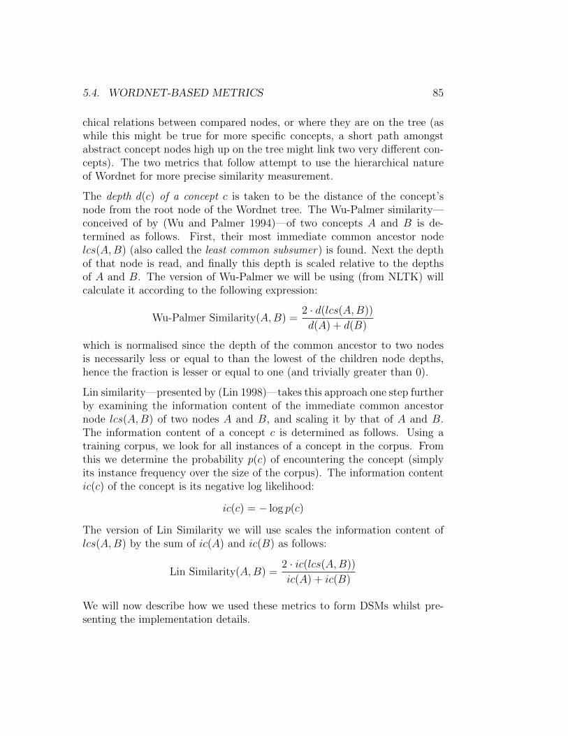
5.4. WORDNET-BASED METRICS 85
chical relations between compared nodes, or where they are on the tree (aswhile this might be true for more specific concepts, a short path amongstabstract concept nodes high up on the tree might link two very different con-cepts). The two metrics that follow attempt to use the hierarchical natureof Wordnet for more precise similarity measurement.
The depth d(c) of a concept c is taken to be the distance of the concept’snode from the root node of the Wordnet tree. The Wu-Palmer similarity—conceived of by (Wu and Palmer 1994)—of two concepts A and B is de-termined as follows. First, their most immediate common ancestor nodelcs(A,B) (also called the least common subsumer) is found. Next the depthof that node is read, and finally this depth is scaled relative to the depthsof A and B. The version of Wu-Palmer we will be using (from NLTK) willcalculate it according to the following expression:
Wu-Palmer Similarity(A,B) =2 · d(lcs(A,B))
d(A) + d(B)
which is normalised since the depth of the common ancestor to two nodesis necessarily less or equal to than the lowest of the children node depths,hence the fraction is lesser or equal to one (and trivially greater than 0).
Lin similarity—presented by (Lin 1998)—takes this approach one step furtherby examining the information content of the immediate common ancestornode lcs(A,B) of two nodes A and B, and scaling it by that of A and B.The information content of a concept c is determined as follows. Using atraining corpus, we look for all instances of a concept in the corpus. Fromthis we determine the probability p(c) of encountering the concept (simplyits instance frequency over the size of the corpus). The information contentic(c) of the concept is its negative log likelihood:
ic(c) = − log p(c)
The version of Lin Similarity we will use scales the information content oflcs(A,B) by the sum of ic(A) and ic(B) as follows:
Lin Similarity(A,B) =2 · ic(lcs(A,B))
ic(A) + ic(B)
We will now describe how we used these metrics to form DSMs whilst pre-senting the implementation details.
86CHAPTER 5. EVALUATING DOCUMENT SIMILARITY MEASURES
5.4.2 Implementing Wordnet-based Metrics
We need not concern ourselves with the mathematics of the metrics de-scribed above, since NLTK’s wordnet module will provide us with the samefunctions as described by (Pedersen et al. 2004) (and also provided in hisWordnet::Similarity Perl module). Our chief task is to get parts of speechof document tokens so as to be able to apply these metrics to them (sincethey only compare nouns to other nouns, and verbs to other verbs, and ignorethe rest), and also conceive of a way of computing the similarity between twodocuments using metrics which will compute the similarity between words,as discussed in §3.2.3.
We began by writing a TAGevaluator subclass of evaluator which wouldextend evaluator’s initialisation by POS-tagging each document from eachcorpus entry and adding the token/tag pairs for each document in each cor-pus entry to eval data, using a standard POS-tagger provided by NLTK(nltk.pos tag()). It would also define a class list called stopwords pop-ulated with English stopwords read from NLTK’s nltk.corpus.stopwords
corpus. The rest of TAGevaluator’s initialisation function is as in evaluator,and calls getscore which calls scoreline in order to evaluate the corpusfor a given metric.
We then wrote a general Wordnet evaluation class—WNevaluator, a subclassof TAGevaluator—which does all the work. It has two attributes, metricand ic, which are both initialised to ‘None’ (‘void type object’ for Python).The idea is that this class would contain all the code necessary to run theevaluation when metric was defined as one of the three Wordnet metrics(and ic pointed to a text to use as information context for Lin Similarity),and that the individual metric classes would need to do nothing more butoverload the value of metric (and of ic, if needed), and implicitly classWNevaluator’s scorecorpus function would be called by getscore duringthe initialisation function, since they would provided none of their own. Ifno metric was provided, WNevaluator will not initialise and will raise andexception.
Thus all that is done in the classes pathsimeval, WUPeval and LINeval—subclasses of WNevaluator standing for Path similarity, Wu-Palmer sim-ilarity, and Lin Similarity respectively—would be to overload metric aspath similarity, wup similarity and lin similarity, respectively (all

5.4. WORDNET-BASED METRICS 87
provided by NLTK’s wordnet module). Additionally, LINeval also over-loads ic by setting it to NLTK’s wordnet ic module object set to retrievethe British National Corpus already processed to serve as an informationcontext (i.e. it is a dictionary mapping concepts to probabilities calculatedfrom the British National Corpus).
The scoreline function common to all these metrics and defined in WNevaluator
works as follows: first it collects all the nouns from both documents fromthe corpus entry passed to it into two lists (one per document), using thegetgroups function which also filters out stopwords listed in class list stopwords.Then it gathers a list of all the concepts from each list and puts them into twodictionaries (one for each document) each mapping nouns to lists of concepts.We create a list of all possible pairs of nouns built picking one noun fromeach document. For each such pair we iterate through concept pairs usingthe noun-to-concept dictionaries and compute the concept similarity usingthe metric specified in metric. The best score for that noun pair is recordedin a dictionary mapping noun-pairs to best concept similarity scores.
The above steps are repeated for all the verbs in each document to obtain adictionary mapping verb-pairs to the similarity measure of the best-matchingconcepts underlying the verbs of that pair. We write the scores from bothdictionaries to a single list, take the top 10% highest scores and averagethem, and thus obtain the document similarity measure for the documentpair. This score is returned to the calling function.
5.4.3 Fine-tuning: How Far is Too Far?
The method described above is fairly fine tuned. Our first scaling attemptwas to collect all the concepts of all the nouns from both documents intotwo lists, take all the concept pairs constructed from taking one conceptfrom each list, compute the similarity of each pair, and average over all thescores. But since there may be a dozen or so other senses for each noun otherthan that in which it was used, this brute-force method performs very poorlybecause most concept-pairs evaluated have nothing to do with the conceptsexpressed in the documents.
Another approach was to take a first sense heuristic, since when retrievingthe concepts underlying a word using Wordnet, the most common senses

88CHAPTER 5. EVALUATING DOCUMENT SIMILARITY MEASURES
are usually the first ones in the list. We therefore could take the sense of aword to be the first one on the list, and proceed as above (now word pairsand concept pairs are effectively the same, since we have one concept perdocument word). This produced slightly better results, but ultimately theywere still much worse than those provided by the ‘top 10%’ heuristic wedescribed in §5.4.2.
The point being made is that more sophisticated scaling heuristics producebetter results. We could doubtlessly do even better. For example, J. Carthy7
suggests using lexical chaining with Wordnet to disambiguate a sentence(mapping words to precise concepts). If effective, this would most likelyproduce better results than our ‘top 10%’ heuristic since it essentially mapswords to their concepts (with some error), and thus we compare conceptsdirectly, as we would for words, and can safely average over the whole bunch.
Why, then, did we not do this? First of all, because it would have takenconsiderably more time to research how to do so correctly, and would involvestraying from the priorities of this experiment by focussing on a small set ofmetrics. But more importantly, as we argued in §3.2.3, we wish to evaluatethe original metrics, rather than our ability to derive new metrics from them.In order to compare the Wordnet-based metrics to other metrics, it was nec-essary to scale them so that they could process the same corpus. However,if the onus for results lay more in the heuristic used to disambiguate docu-ment words rather than evaluating their similarity, we would be performinga different task from that which was originally intended.
5.5 Semantic Vectors
In this section, we present the concept of distributional measures of semanticsimilarity, and show how we used a vector-base approach to distributionalsimilarity measurement using a package designed by (Widdows and Ferraro2008) to implement this metric.
7cf. Short bibliographical overview at http://www.csi.ucd.ie/staff/jcarthy/home/Lex.html.

5.5. SEMANTIC VECTORS 89
5.5.1 Background Theory
Although the origin of distributional semantic similarity measures is usuallyattributed to (Firth 1957) (cf. §2.2.3 and §2.2.4) we argued in §2.3 that itsorigin was more likely the ‘meaning-is-use’ presented by (Wittgenstein 1953).The idea is to determine the semantics of a word by looking at other wordsused alongside it in English sentences.
One way of doing this is to use vectors to represent word senses, and to usecosine similarity of two vectors to compute the semantic similarity of thewords they stand for. First, one must build a set of vectors for each word inour n-entries lexicon8. The vectors are set in an n-dimensional orthogonalvector space where each basis is assigned a unique lexicon word (hence eachlexicon entry has a basis in the vector space). For each word in the lexicon,a vector is determined in this space, where the vector component for eachbasis is the number of instances the word the basis stands for appears in thecontext of the word a vector is being constructed for. ‘Context’ here can beas general as the word appearing in the same document, or as specific as somemore fine-grained definition, such as that used by (Grefenstette 1992), whosuggests using words with some grammatical relation to the target words toconstruct vectors (e.g. adjectives modifying the word, verbs it is the subjectof, etc.). During this operation, we naturally ignore the cases of a wordco-occuring with itself.
The similarity between two words is then determined by taking the cosinecomponent of their vectors’ product. If words A and B have vectors vA andvB, then the semantic similarity sim(A,B) is simply:
sim(A,B) =vA · vB|vA| · |vB|
which is normalised, since it is just a cosine reading of the unit vector com-ponent of vA and vB, which is a real number between 0 and 1.
To give a short example, let us suppose the only words in our keyword lexiconare ‘cat’, ‘kitten’ and ‘dog’. We read that ‘kitten’ co-occurs with ‘cat’ in 12documents, and with dog in only 3. We consider a vector space with only‘dog’ and ‘cat’ as basis vectors, in which the vector kitten would be 3 times
8Usually stopwords and common verbs (if not already in the stopword list) are removedfrom the lexicon, since they do not aid sense disambiguation much, being frequently present
90CHAPTER 5. EVALUATING DOCUMENT SIMILARITY MEASURES
the ‘dog’ basis vector, and 12 times the ‘cat’ basis vector, thus its similaritywith the ‘cat’ basis vector would be:
sim(kitten, cat) =3 · 0 + 12 · 1√
32 + 122 · 1=
12√153≈ 0.97
while its similarity with the ‘dog’ basis vector would be:
sim(kitten, dog) =3 · 1 + 12 · 0√
32 + 122 · 1=
3√153≈ 0.24
hence showing us that document co-occurrence has sufficed to show us that‘kitten’ is closer to ‘cat’ than to ‘dog’ since it appears in the same context asthe former more often than that of the latter.
5.5.2 Implementation: A Different Approach to Word-Sentence Scaling
The implementation of this metric was a bit more complicated than the pre-vious ones. We used the SemanticVectors packaged developed by (Widdowsand Ferraro 2008), which a Java library (the rest of our project is in Python).The SemanticVectors package provides a set of function used for buildingthe vectors from a corpus, and helper functions for computing the scalarproduct of two vectors. Using these, and a script we provided to extract aplain-text version of the American National Corpus, Pascal Combescot, whowas working on a similar project, provided us with a Java script which weadapted9 into a command-line script taking two document files as argumentsand returning their semantic similarity, as well as a vector set to use for eval-uation based on the ANC. The source for this program has been reproducedin §B.5.
The reader may wonder how we integrated this into our evaluation classes,and more importantly: how did we compare documents in this manner whenthis vector-based distributional metric was designed to compare the meaningof words? To answer the second question, we simply took the vector of adocument to be the sum of all the vectors standing for words contained in
9We re-wrote under half of the main function shown in §B.5 to adapt the class to ourpurposes. The rest of this Java package was written by Pascal Combescot.

5.5. SEMANTIC VECTORS 91
the document (if words have no vectors, they are ignored). This gave goodempirical results in Pascal’s project, so we adapted this method here too.The obvious downside is that while fairly effective, it is fundamentally flawed:vector addition is commutative, hence for any words A and B, vA + vB =vB + vA. Therefore the vector for ‘The dog bit the man’ would be the sameas that of ‘The man bit the dog’, effectively assigning them an identical senseeven though the meaning obviously differs. However, this heuristic workedwell enough, so we were curious to see how it would compare to other metricsand used it as such.
Finally, to integrate the measure into our evaluation system, we wrote SemVecteval,a subclass of evaluator. It overloads getscore (instead of the usual scorelinefunction). For each corpus entry, it writes the documents of the entry’s doc-ument pair to two separate temporary files, the names of which it records inan index file along the ID of the entry. Once it has done this for each entry inthe corpus, it passes the index file to the SemanticVectorsEvaluator Javacommand-line program based on Pascal’s script described above, which com-putes the document similarity of each document pair in the corpus, writesit to a file mapping IDs to scores, which getscore reads once the process iscompleted in order to recover the metric scores, which it then stores in theusual scores dictionary mapping IDs to metric scores, which it returns tothe initialisation function.

92CHAPTER 5. EVALUATING DOCUMENT SIMILARITY MEASURES

Chapter 6
Results and Analysis
In this chapter we will first briefly describe, in §6.1, how the analysis scriptwas implemented according to the specifications discussed in §3.3. Follow-ing that, in §6.2 we will present the metric rankings and examine the CGSscore breakdown—first discussed in §3.3.2—of a few metrics for the corpuscategories where the scores were interesting or surprising.
6.1 Structure of Analysis Script
The analysis script—analyser.py—is a command-line utility which essen-tially takes a data file containing the results of evaluating all the metricsusing the classes discussing in Chapter 5, and produces a file containing themetric rankings, as well as a series of other files. Its source code is presentedin §B.7. The class takes as input a dictionary results mapping metrics todictionaries which in turn map IDs to the metric CGS score for the corpusentries with those IDs. In short, to retrieve a DSM metric CGS score forcorpus entry ID, one would call results[metric][ID].
As discussed in §4.1.1, the ID for each corpus entry tells us which corpussection it is from, as well as what subsection (if any) and if it was gen-erated by mismatching documents (mixed corpus entries) based a ‘(COR-PUS SECTION) [-SUBSECTION TAG] (ID NUMBER) [m]’ structure. Weuse the information in the ID tags for all the corpus entries in results to pop-
93

94 CHAPTER 6. RESULTS AND ANALYSIS
ulate three dictionaries, cats, matchcats and mixedcats which will mapcategory names to lists of IDs of corpus entries in those categories, with thehelp of regexes exploiting the structure of the tags. The difference betweenthese dictionaries is:
• cats maps categories to lists of all the IDs of corpus entries in thosecategories.
• matchcats maps categories to lists of all the IDs of corpus entries inthose categories which were generated by the corpus constructors (i.e.non-mixed).
• mixedcats does as above, but the IDs are those of corpus entries gen-erate through mixing.
These three dictionaries are passed, with results, one by one, to the func-tion getcatscores which assembles a dictionary mapping metrics to dictio-naries mapping categories to dictionaries mapping tags to CGS scores. Thedictionaries are stored in catscores, matchcatscores and mixedcatscores.They are essentially results with some extra classification: e.g. matchcatscores[metric][category]gives you a dictionary mapping all the IDs in the category category to CGSscores for DSM metric.
These three new dictionaries are then passed, one by one, to getmetricAVGs
which returns three separate dictionaries—metricAVGs, matchmetricAVGs
and mixedmetricAVGs—mapping categories to dictionaries mapping metricsto their average CGS score for that category. To clarify, if one wanted theaverage CGS score of DSM metric for documents of category cat, but onlythose produced by mixing, one would call mixedmetricsAVGs[cat][metric].If one wanted the average CGS score for all documents in the category, onewould call metricsAVGs[cat][metric].
These dictionaries are first passed to the function publishAVGs which pub-lishes the CGS averages per category per metric to a specified file (results.txtin our experiment). Next they are passed to the function publishDists
which for each category, for each metric, publishes plots of the distributionof CGS scores for that metric, for documents of that category. We usedMatplotlib’s pylab1 wrapper to achieve this.
The final step is to calculate metric differences—the MD score, as discussed
1Obtained from http://matplotlib.sourceforge.net/.
6.2. DISCUSSION OF METRIC CGS SCORES 95
in §3.3.2. A list of all possible metric pairs is written to metricpairs. Foreach metric pair, the absolute difference between the metric CGS scores foreach corpus document pair is written to the dictionary metricdiffs map-ping metric pairs to dictionaries mapping corpus IDs to MD scores for thatmetric pair, for those corpus items. This dictionary is then used to publishthe ranked MD scores to a text file (metricdiffs.txt in our experiment)using publishDiffs, a variant of publishDists. It also plots the distri-bution of MD scores for each metric pair, for each corpus section, usingpublishDiffDists, a variant of publishDists.
6.2 Discussion of Metric CGS Scores
The full rankings for average CGS scores per corpus section and per DSMare tabulated in the Tables 6.2–6.4. The totality of plots generated by theanalysis script as well as the MD score rankings per corpus section and permetric pair are not provided here2, as there are 2457 plots (338 for CGSscore distributions, 2094 for metric comparisons) and a large number of MDrankings (namely the number of DSMs squared times the number of testbedcorpus sections). In this section, we will discuss the CGS score rankings, anddisplay charts where interesting results were found. We will leave discussionof how to exploit metric comparison scores for the conclusion.
6.2.1 Overall Rankings
As stated above, our experiment generates 338 plots3, which is too manyto examine each one individually. We will be relying on a the rankings toidentify metrics which require closer investigation for certain corpus sections.
We have reproduced the CGS scores as percentages (i.e. we multiply theCGS score by 100 and round to the second decimal place) of closeness to a
2All files used for and generated by this experiment will be provided on an accompa-nying CD-ROM. See Appendix A for details.
313 metrics times 9 document sections times 3 class of comparison (all corpus entries,only those generated by constructors, only those generated by mixing), minus the 13 entriesfor the mixed comparison class for the random edits corpus, which does not generate amixed class (cf. §4.2.2).

96 CHAPTER 6. RESULTS AND ANALYSIS
Key Corpus Category1 Abstracts2 Edits3 POSswitch4 Paraphrase5 Paraphrase [MTC]6 Paraphrase [News]7 Paraphrase [Novel]8 Themes9 Wikipedia
Table 6.1: Corpus Category Legend
perfect evaluator in Tables 6.2, 6.3 and 6.44. Hence a metric with a scoreof 89.02% for some corpus section is 82.02% as effective as a perfect DSMin identifying the kind of similarity that section exemplifies. For formattingreasons, the corpus section names in these tables were replaced by numbers.Refer to Table 6.1 to match numbers to corpus section names.
We will go through the rankings corpus section by corpus section. Notablescores will be highlighted in the score tables when referred to.
6.2.2 Random Edits Analysis
First up is the random edits section (cf. §4.2.2). We note that the Leven-shtein edit distance scores well for all documents at over 90% CGS in Table6.2. Looking at Figure 6.1 gives us a good example of what good metricresults look like, with a majority of metric CGS scores for the individualsection entries being very close to 1.0. This is unsurprising, since the editsused to generate the corpus are the exact same the Levenshtein edit distancetracks. Ratio similarity, as discussed in §5.2.4, makes use of the Levenshteinedit distance in addition to the size of the strings, so it is normal to find it insecond place with a score of 82.64%. Jaro-Winkler distance also works well
4We note the absence of corpus section 2 (random edits) in this table. This is becauseall the corpus entries for this section were generated by the corpus builder, and no mixingtook place. As such, the scores in the matched document scores table (cf. Table 6.3) arethe same as in the overall scores table (cf. Table 6.2).
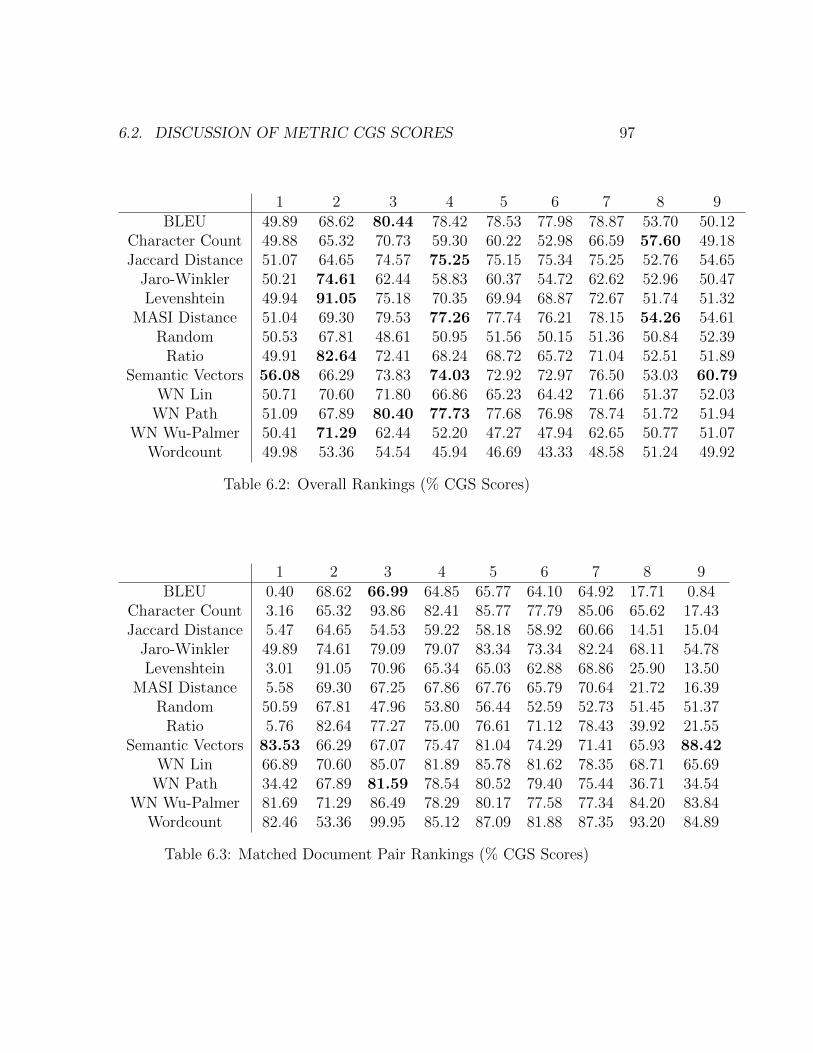
6.2. DISCUSSION OF METRIC CGS SCORES 97
1 2 3 4 5 6 7 8 9BLEU 49.89 68.62 80.44 78.42 78.53 77.98 78.87 53.70 50.12
Character Count 49.88 65.32 70.73 59.30 60.22 52.98 66.59 57.60 49.18Jaccard Distance 51.07 64.65 74.57 75.25 75.15 75.34 75.25 52.76 54.65
Jaro-Winkler 50.21 74.61 62.44 58.83 60.37 54.72 62.62 52.96 50.47Levenshtein 49.94 91.05 75.18 70.35 69.94 68.87 72.67 51.74 51.32
MASI Distance 51.04 69.30 79.53 77.26 77.74 76.21 78.15 54.26 54.61Random 50.53 67.81 48.61 50.95 51.56 50.15 51.36 50.84 52.39
Ratio 49.91 82.64 72.41 68.24 68.72 65.72 71.04 52.51 51.89Semantic Vectors 56.08 66.29 73.83 74.03 72.92 72.97 76.50 53.03 60.79
WN Lin 50.71 70.60 71.80 66.86 65.23 64.42 71.66 51.37 52.03WN Path 51.09 67.89 80.40 77.73 77.68 76.98 78.74 51.72 51.94
WN Wu-Palmer 50.41 71.29 62.44 52.20 47.27 47.94 62.65 50.77 51.07Wordcount 49.98 53.36 54.54 45.94 46.69 43.33 48.58 51.24 49.92
Table 6.2: Overall Rankings (% CGS Scores)
1 2 3 4 5 6 7 8 9BLEU 0.40 68.62 66.99 64.85 65.77 64.10 64.92 17.71 0.84
Character Count 3.16 65.32 93.86 82.41 85.77 77.79 85.06 65.62 17.43Jaccard Distance 5.47 64.65 54.53 59.22 58.18 58.92 60.66 14.51 15.04
Jaro-Winkler 49.89 74.61 79.09 79.07 83.34 73.34 82.24 68.11 54.78Levenshtein 3.01 91.05 70.96 65.34 65.03 62.88 68.86 25.90 13.50
MASI Distance 5.58 69.30 67.25 67.86 67.76 65.79 70.64 21.72 16.39Random 50.59 67.81 47.96 53.80 56.44 52.59 52.73 51.45 51.37
Ratio 5.76 82.64 77.27 75.00 76.61 71.12 78.43 39.92 21.55Semantic Vectors 83.53 66.29 67.07 75.47 81.04 74.29 71.41 65.93 88.42
WN Lin 66.89 70.60 85.07 81.89 85.78 81.62 78.35 68.71 65.69WN Path 34.42 67.89 81.59 78.54 80.52 79.40 75.44 36.71 34.54
WN Wu-Palmer 81.69 71.29 86.49 78.29 80.17 77.58 77.34 84.20 83.84Wordcount 82.46 53.36 99.95 85.12 87.09 81.88 87.35 93.20 84.89
Table 6.3: Matched Document Pair Rankings (% CGS Scores)

98 CHAPTER 6. RESULTS AND ANALYSIS
0.0 0.2 0.4 0.6 0.8 1.0Closeness to gold standard
[Higher is better]
0
10
20
30
40
50
Num
ber
of occ
urr
ence
s
Edits Corpus (Overall)Score difference distribution for metric: Levenshtein Edit Distance
Figure 6.1: Levenshtein Edit Distance CGS Score Distribution (Edits Sec-tion)
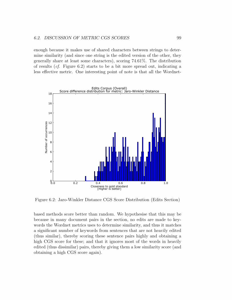
6.2. DISCUSSION OF METRIC CGS SCORES 99
enough because it makes use of shared characters between strings to deter-mine similarity (and since one string is the edited version of the other, theygenerally share at least some characters), scoring 74.61%. The distributionof results (cf. Figure 6.2) starts to be a bit more spread out, indicating aless effective metric. One interesting point of note is that all the Wordnet-
0.0 0.2 0.4 0.6 0.8 1.0Closeness to gold standard
[Higher is better]
0
2
4
6
8
10
12
14
16
18
Num
ber
of occ
urr
ence
s
Edits Corpus (Overall)Score difference distribution for metric: Jaro-Winkler Distance
Figure 6.2: Jaro-Winkler Distance CGS Score Distribution (Edits Section)
based methods score better than random. We hypothesise that this may bebecause in many document pairs in the section, no edits are made to key-words the Wordnet metrics uses to determine similarity, and thus it matchesa significant number of keywords from sentences that are not heavily edited(thus similar), thereby scoring these sentence pairs highly and obtaining ahigh CGS score for these; and that it ignores most of the words in heavilyedited (thus dissimilar) pairs, thereby giving them a low similarity score (andobtaining a high CGS score again).

100 CHAPTER 6. RESULTS AND ANALYSIS
6.2.3 POS-Switch Analysis
The other syntactic toy-corpus section, POS-Switch (cf. §4.2.3), yields twoparticularly interesting results which exemplify proper analysis methodology.The top-two ranking metrics are BLEU and Wordnet Path similarity, bothscoring highly in Table 6.2. We hypothesise that this is for roughly thesame reasons as in the random edit corpus: dissimilar sentence pairs withmany substitutions will score poorly on the BLEU metric (since one pair isthe reference translation for the other, and randomly substituted words arebound to lower the BLEU score, as well as the Path Similarity since they areunlikely to be lexically related to the word they replace). At face value, theymay look the same, but further analysis tells us otherwise: if we look at theentries for these metrics in the POS-switch section of Tables 6.3 and 6.4, wenotice that while the score for Path Similarity in both these tables is roughlythe same as the original, the score for BLEU is considerably lower for matchdocuments, and higher for mixed (mismatched) documents, suggesting thatBLEU picks up more strongly on some characteristic which affects documentsimilarity but doesn’t fully determine it. The score disparity is especiallyevident when one looks at the breakdown of score distributions for bothmetrics.
For the overall score distribution, seen in Figure 6.3, we note that althoughBLEU has a high CGS score density in the high-score bracket (above 0.8),it also has a has a more significant distribution of scores across the scorerange. Path Similarity, on the other hand, has a very sharp spike for thetop score (meaning the CGS score for almost all section documents is 1.0).It, however, makes more drastic errors for a set of documents (notice thespike at the 0 CGS score point). When we examine how the metrics performfor the matched section entries in Figure 6.4, there is not much change tothe CGS score distribution for Path Similarity, however we observe that theCGS scores for BLEU are spread widely across the centre of the score range,with several sharp spikes at CGS values inferior to 0.5. Finally when weexamine how the metrics perform for the mixed section entries in Figure6.5, we see a heavy concentration of high scores for BLEU, while the scoredistribution for Path Similarity retains the same shape. We judge from thisthat document features causing lowering of CGS scores for Path Similarity aredissociated from those used to assess similarity by Path Similarity, whereasBLEU correctly identifies features that make documents dissimilar, but is

6.2. DISCUSSION OF METRIC CGS SCORES 101
not as good at identifying similar documents, and thus is exploiting featuresthat don’t solely determine similarity. The result of this in-depth analysis isthat although both DSMs achieve similar performance in this testbed sectionat first blush, graphical analysis of the CGS score distributions allow us toassess that Path Similarity is a better metric for this corpus section thanBLEU.
6.2.4 Theme Analysis
We now move on to our lexical similarity section—the Theme section (cf.§4.3). This corpus section produces no truly interesting results, given themetrics we evaluated. However, the top two metrics do have interestingscore distributions which we will use to illustrate the danger of thinking thata metric with a higher average CGS score is necessarily a more sophisticatedone. As can be seen in Table 6.2, character count scores 57.60% CGS, a fewpercentage points ahead of MASI distance, which scores 54.26%. However,consider the section CGS score distributions for these metrics, shown in Fig-ure 6.6. We see that character count’s CGS score distribution is close, inshape, to that of the Random Evaluator, also shown in Figure 6.6. This canserve as an indication that character count’s high performance in this testis possibly a fluke and that it assigns metric scores fairly randomly. Thisintuition is confirmed by our knowledge of character count’s modus operandiand the fact that although the chunks of paragraphs in the Theme section ofthe corpus are roughly the same length, there is much room for divergencein character count between the two documents of a corpus entry. The pointhere is that we could have deduced that the metric does not exploit anypragmatically significant features of documents relative to the type of simi-larity (namely lexical) we are concerned with, even if we had no knowledgeof how the metric works or the structure of the corpus section. On the otherhand, MASI forms two neat clusters in high-scoring and low-scoring regionsof the plot, indicating it at least exploits some property common to all itemsof the corpus, but doesn’t necessarily play a significant role in determiningsimilarity. This thus gives us information about how metrics of this sortmight function even without knowing its internal mechanisms, and also tellsus that it might serve as a possible component for hybrid metrics, somethingCharacter Count obviously would not be suitably for, with regards to thetype of similarity expressed in this corpus section.

102 CHAPTER 6. RESULTS AND ANALYSIS
6.2.5 Wikipedia Analysis
Next we examine the results of DSMs tested against the Wikipedia articlecorpus (cf. §4.4). This was a difficult corpus section, since articles were pairedby subject and thus by loose lexical/semantic similarity, but the structuraland lexical correspondence between the articles varies widely. As can besee in Table 6.2, no metric does particularly well. However, analysis of theCGS score distribution for the leading DMS—Semantic Vector Similarity(60.79%) can give us some indication as to how we could construct metricscapable of dealing with this corpus section (something the rankings alonedon’t tell us). Figure 6.7a shows two groupings of CGS scores: a high densitygrouping of entries with high (over 0.8) scores, and a spread of moderatelylow scores (in the 0.15 to 0.6 range). Contrary to the symmetric twin spikesobserved for MASI, for the Theme section (cf. Figure 6.6b), the groupingshere are largely asymmetric relative to one another. Also unlike the MASIcase, a look at the score distributions for matched and mixed documentsonly (cf. Figures 6.7b and 6.7c, respectively) tells us that the SemanticVectors metric is very good at detecting similarity for matched cases, makingfew mistakes (Figure 6.7b), but is also latching onto some similar featuresfor the dissimilar cases, although not as strongly, since the distribution oferrors in Figure 6.7b is broad and spreads into the better-than-random classof scores (over 0.5). This indicates that at least some of the propertiessemantic vector similarity is exploiting to judge similarity are present in theother documents. This, combined with our knowledge of how semantic vectorsimilarity works could help us design a new metric for this sort of similarity.We know that the semantic vector metric adds up the word-vectors of allnon-stopwords to build document vectors, which are then compared usingcosine similarity. The problem, we can infer from the CGS breakdowns, isthat there are some words being used to build document vectors which arein too many of the Wikipedia articles and are playing an unwanted role inthe comparison of mismatched articles. We could fix this in several ways.One way we suggest would be to determine what non-stopwords are frequentthroughout the Wikipedia corpus (what ‘frequent’ means here would haveto be empirically determined, we suppose) and add these to the stopwordlist, since this ‘lexical baseline’ offers no significant contribution to similarityjudgements. Naturally this sort of conclusion could be arrived at throughthinking about how the metric works and how the corpus is structured in the

6.2. DISCUSSION OF METRIC CGS SCORES 103
first place, but this example seeks to illustrate how graphical CGS analysissimplifies the task for us.
6.2.6 Paraphrase Analysis
We then look into the results for the Paraphrase section of the corpus (cf.§4.5) and its subsections. We read from Table 6.2 that the top scoring met-rics are BLEU, Path Similarity, MASI and Jaccard Distances, and SemanticVector Similarity, all scoring well above 70%. Levenshtein also does signifi-cantly better than random, scoring 70.35% overall. The is a lot to say here:let us begin by setting BLEU aside. Its high performance for paraphrase onthe whole is no surprise, since it is designed to evaluate paraphrase generatedthrough translation (which is what constitutes two subsections of the Para-phrase corpus section), and therefore it is not unexpected that it work wellas an evaluator for general paraphrase as provided in the MTC subsection.
Let us instead focus on the other two syntactic metrics. Analysis of bothof these metrics is straightforward. We look at the overall score distributionof both metrics in Figure 6.8 and notice that there is a high spike towards1.0 CGS for both metrics, and that almost all the rest of the scores arein the high end of the 0.5–1.0 range, indicating that the metric probablyscoring fairly consistently, i.e. that it predominantly exploits properties thatdetermine similarity to produce its own judgement of similarity. All oneneeds is a quick glance at Figures 6.9 and 6.10 to confirm this, as we observethat the distribution of the CGS scores is the of the same shape as the overalldistribution for both metrics, indicating that neither metric strongly relieson document properties that do not affect classification, since it makes nosignificant consistent error in either case (as is the case for metrics showingsymmetrically opposed groupings in the overall distribution). In both cases,visual analysis quickly tells us that both DSMs are well designed for such asimilarity type, and that better results are most likely to be obtained throughimproved heuristics in the metric design.
The ‘surprises’ in this corpus section are the performances of some of the syn-tactic measures. Let’s examine the two top: MASI and Jaccard Distances.A quick glance through the CGS score distributions for overall, mixed andmatched document pairs in Figures 6.11, 6.12 and 6.13 shows distributionsthat are fairly similar in shape and high-score density to the distributions

104 CHAPTER 6. RESULTS AND ANALYSIS
for semantic vector similarity and path similarity. Furthermore, we observethat the shapes of the distributions when considering only the matched andmixed documents are, in both instances, roughly the same as for the overalldistribution (much like semantic vector similarity and path similarity’s distri-butions were). We therefore can draw the same conclusions as for semanticvector similarity and path similarity: these metrics, which we previouslythought to be purely syntactic, actually exploit document properties thatare similarity features. Now, if we think back about how both these metricswork, they merely compute the intersection of sets of tokens (one for eachdocument) and normalise it by the size of the union of the sets or by the sizeof the largest set for Jaccard Distance and MASI distance, respectively. Wecan hypothesise that when paraphrasing sentences, the structure does notchange much, hence certain stop words are likely to occur no matter how werephrase key words. Other words such as names are unlikely to change duringparaphrase, and certain verbs and nouns may be present in both documents,hence MASI and Jaccard scores for paraphrase document pairs often comeclose the gold-standard score despite not being designed to track semantic orlexical properties.
That MASI and Jaccard distances could be used in such a way is fairlycounter-intuitive, but the fact that they produce results on par with semanticmetrics goes to show there is some evidence in support of the Wittgensteinianidea of abolishing distinctions between document similarity categories, asdiscussed in §2.3. Also, it illustrates how this analysis framework is powerfulin both discovering new uses for metrics, and assessing their performance inmore detail, guiding our explanations as to how they produce unexpectedlygood results.
6.2.7 Abstract-Article Analysis
Finally we consider the abstract-article section of the corpus (cf. §4.6). Forthis testbed section, we will be brief, as none of the metrics have performedmuch better than the random evaluator. The only metric which stands outis Semantic Similarity.
As shown in Figure 6.14, the CGS score distribution for semantic vectorsimilarity shows the characteristic symmetrically-opposed groupings that in-dicate that whatever properties the metric is exploiting aren’t fully connected

6.2. DISCUSSION OF METRIC CGS SCORES 105
to similarity features, and are a cause of consistent misclassification. A quickglance at the score disparity between mixed document score (83.53%) andmatched document score (28.64%) in Tables 6.3 and 6.4, respectively, pro-vides us with information to determine the cause. The problem is similar tothat which Semantic Vector similarity faced in the Wikipedia corpus: thereis a ‘baseline’ vocabulary shared by most papers from the same subject ordomain, which will be contribute to the document vectors of most documentsand abstracts. As a result, Semantic Vector Similarity is very good at de-tecting similar documents, but concludes that even dissimilar documents aresimilar because they possess baseline vocabulary features. With the knowl-edge, DSM designers can consider the same approach we suggested for theWikipedia corpus, and design metrics which identify shared vocabulary andignore it (or give it less impact during assessment) before assessing similarity.

106 CHAPTER 6. RESULTS AND ANALYSIS
1 3 4 5 6 7 8 9BLEU 99.39 93.88 91.99 91.30 91.86 92.83 89.68 99.40
Character Count 96.59 47.60 36.19 34.66 28.17 48.13 49.58 80.93Jaccard Distance 96.67 94.61 91.28 92.12 91.75 89.83 91.02 94.27
Jaro-Winkler 50.52 45.80 38.59 37.40 36.11 43.00 37.82 46.16Levenshtein 96.88 79.40 75.35 74.86 74.86 76.47 77.58 89.15
MASI Distance 96.51 91.81 86.66 87.72 86.63 85.65 86.80 92.82Random 50.48 49.27 48.09 46.68 47.72 49.99 50.24 53.42
Ratio 94.06 67.56 61.48 60.82 60.31 63.65 65.10 82.24Semantic Vectors 28.64 80.59 72.59 64.80 71.66 81.58 40.13 33.16
WN Lin 34.54 58.53 51.83 44.67 47.22 64.97 34.02 38.36WN Path 67.75 79.21 76.91 74.84 74.56 82.04 66.74 69.33
WN Wu-Palmer 19.13 38.39 26.10 14.37 18.31 47.96 17.34 18.29Wordcount 17.50 9.14 6.76 6.29 4.78 9.81 9.29 14.96
Table 6.4: Mixed Document Pair Rankings (% CGS Scores)

6.2. DISCUSSION OF METRIC CGS SCORES 107
0.0 0.2 0.4 0.6 0.8 1.0Closeness to gold standard
[Higher is better]
0
10
20
30
40
50
60
70
Num
ber
of occ
urr
ence
s
POSswitch Corpus (Overall)Score difference distribution for metric: BLEU Similarity
(a) BLEU CGS Distribution
0.0 0.2 0.4 0.6 0.8 1.0Closeness to gold standard
[Higher is better]
0
50
100
150
200
250
300
350
400
450
Num
ber
of occ
urr
ence
s
POSswitch Corpus (Overall)Score difference distribution for metric: WN Path Similarity
(b) Path Similarity CGS Distribution
Figure 6.3: Comparison of BLEU and Path Similarity for POS-switch Doc-uments
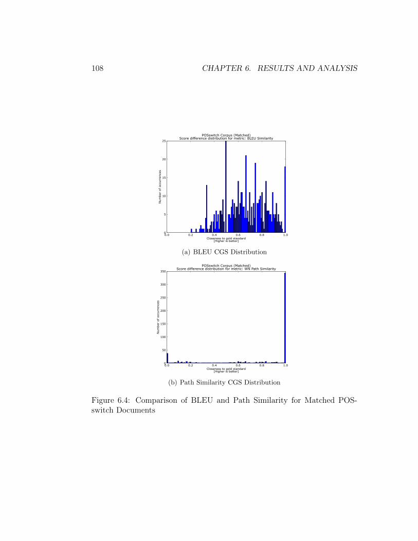
108 CHAPTER 6. RESULTS AND ANALYSIS
0.0 0.2 0.4 0.6 0.8 1.0Closeness to gold standard
[Higher is better]
0
5
10
15
20
25
Num
ber
of occ
urr
ence
s
POSswitch Corpus (Matched)Score difference distribution for metric: BLEU Similarity
(a) BLEU CGS Distribution
0.0 0.2 0.4 0.6 0.8 1.0Closeness to gold standard
[Higher is better]
0
50
100
150
200
250
300
350
Num
ber
of occ
urr
ence
s
POSswitch Corpus (Matched)Score difference distribution for metric: WN Path Similarity
(b) Path Similarity CGS Distribution
Figure 6.4: Comparison of BLEU and Path Similarity for Matched POS-switch Documents

6.2. DISCUSSION OF METRIC CGS SCORES 109
0.0 0.2 0.4 0.6 0.8 1.0Closeness to gold standard
[Higher is better]
0
5
10
15
20
25
30
Num
ber
of occ
urr
ence
s
POSswitch Corpus (Mixed)Score difference distribution for metric: BLEU Similarity
(a) BLEU CGS Distribution
0.0 0.2 0.4 0.6 0.8 1.0Closeness to gold standard
[Higher is better]
0
10
20
30
40
50
60
70
80
90
Num
ber
of occ
urr
ence
s
POSswitch Corpus (Mixed)Score difference distribution for metric: WN Path Similarity
(b) Path Similarity CGS Distribution
Figure 6.5: Comparison of BLEU and Path Similarity for Mixed POS-switchDocuments

110 CHAPTER 6. RESULTS AND ANALYSIS
0.0 0.2 0.4 0.6 0.8 1.0Closeness to gold standard
[Higher is better]
0
2
4
6
8
10
12
Num
ber
of occ
urr
ence
s
Themes Corpus (Overall)Score difference distribution for metric: Character Count
(a) Character Count CGS Distribution
0.0 0.2 0.4 0.6 0.8 1.0Closeness to gold standard
[Higher is better]
0
5
10
15
20
25
Num
ber
of occ
urr
ence
s
Themes Corpus (Overall)Score difference distribution for metric: Masi Distance
(b) MASI CGS Distribution
0.0 0.2 0.4 0.6 0.8 1.0Closeness to gold standard
[Higher is better]
0
2
4
6
8
10
12
Num
ber
of occ
urr
ence
s
Themes Corpus (Overall)Score difference distribution for metric: Random Evaluation
(c) Random Evaluator CGS Distribution
Figure 6.6: Comparison of Character Count and MASI for Theme Documents
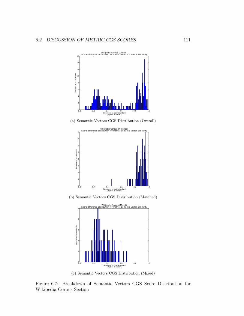
6.2. DISCUSSION OF METRIC CGS SCORES 111
0.0 0.2 0.4 0.6 0.8 1.0Closeness to gold standard
[Higher is better]
0
2
4
6
8
10
12
14
16
Num
ber
of occ
urr
ence
s
Wikipedia Corpus (Overall)Score difference distribution for metric: Semantic Vector Similarity
(a) Semantic Vectors CGS Distribution (Overall)
0.0 0.2 0.4 0.6 0.8 1.0Closeness to gold standard
[Higher is better]
0
1
2
3
4
5
6
7
8
Num
ber
of occ
urr
ence
s
Wikipedia Corpus (Matched)Score difference distribution for metric: Semantic Vector Similarity
(b) Semantic Vectors CGS Distribution (Matched)
0.0 0.2 0.4 0.6 0.8 1.0Closeness to gold standard
[Higher is better]
0
1
2
3
4
5
Num
ber
of occ
urr
ence
s
Wikipedia Corpus (Mixed)Score difference distribution for metric: Semantic Vector Similarity
(c) Semantic Vectors CGS Distribution (Mixed)
Figure 6.7: Breakdown of Semantic Vectors CGS Score Distribution forWikipedia Corpus Section
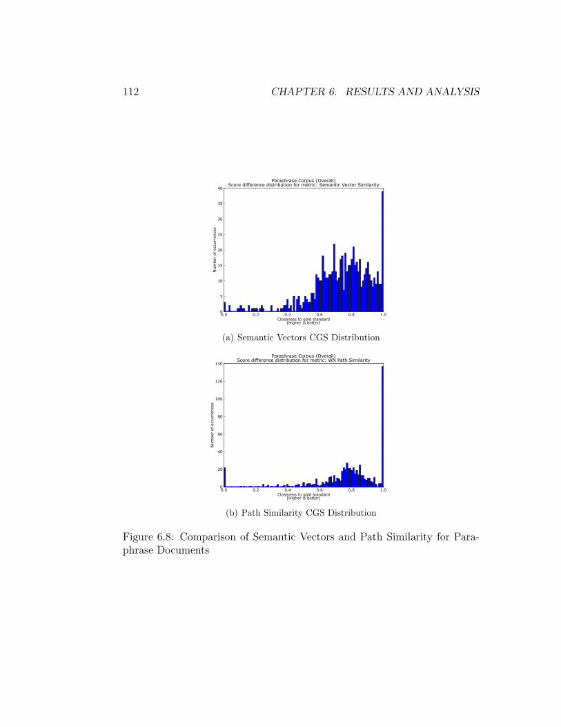
112 CHAPTER 6. RESULTS AND ANALYSIS
0.0 0.2 0.4 0.6 0.8 1.0Closeness to gold standard
[Higher is better]
0
5
10
15
20
25
30
35
40
Num
ber
of occ
urr
ence
s
Paraphrase Corpus (Overall)Score difference distribution for metric: Semantic Vector Similarity
(a) Semantic Vectors CGS Distribution
0.0 0.2 0.4 0.6 0.8 1.0Closeness to gold standard
[Higher is better]
0
20
40
60
80
100
120
140
Num
ber
of occ
urr
ence
s
Paraphrase Corpus (Overall)Score difference distribution for metric: WN Path Similarity
(b) Path Similarity CGS Distribution
Figure 6.8: Comparison of Semantic Vectors and Path Similarity for Para-phrase Documents

6.2. DISCUSSION OF METRIC CGS SCORES 113
0.0 0.2 0.4 0.6 0.8 1.0Closeness to gold standard
[Higher is better]
0
5
10
15
20
25
30
Num
ber
of occ
urr
ence
s
Paraphrase Corpus (Matched)Score difference distribution for metric: Semantic Vector Similarity
(a) Semantic Vectors CGS Distribution
0.0 0.2 0.4 0.6 0.8 1.0Closeness to gold standard
[Higher is better]
0
20
40
60
80
100
120
Num
ber
of occ
urr
ence
s
Paraphrase Corpus (Matched)Score difference distribution for metric: WN Path Similarity
(b) Path Similarity CGS Distribution
Figure 6.9: Comparison of Semantic Vectors and Path Similarity for MatchedParaphrase Documents

114 CHAPTER 6. RESULTS AND ANALYSIS
0.0 0.2 0.4 0.6 0.8 1.0Closeness to gold standard
[Higher is better]
0
2
4
6
8
10
12
Num
ber
of occ
urr
ence
s
Paraphrase Corpus (Mixed)Score difference distribution for metric: Semantic Vector Similarity
(a) Semantic Vectors CGS Distribution
0.0 0.2 0.4 0.6 0.8 1.0Closeness to gold standard
[Higher is better]
0
5
10
15
20
25
30
Num
ber
of occ
urr
ence
s
Paraphrase Corpus (Mixed)Score difference distribution for metric: WN Path Similarity
(b) Path Similarity CGS Distribution
Figure 6.10: Comparison of Semantic Vectors and Path Similarity for MixedParaphrase Documents

6.2. DISCUSSION OF METRIC CGS SCORES 115
0.0 0.2 0.4 0.6 0.8 1.0Closeness to gold standard
[Higher is better]
0
5
10
15
20
25
30
35
40
Num
ber
of occ
urr
ence
s
Paraphrase Corpus (Overall)Score difference distribution for metric: Jaccard Distance
(a) Jaccard Distance CGS Distribution
0.0 0.2 0.4 0.6 0.8 1.0Closeness to gold standard
[Higher is better]
0
5
10
15
20
25
30
Num
ber
of occ
urr
ence
s
Paraphrase Corpus (Overall)Score difference distribution for metric: Masi Distance
(b) MASI Distance CGS Distribution
Figure 6.11: Comparison of Jaccard Distance and MASI Distance for Para-phrase Documents

116 CHAPTER 6. RESULTS AND ANALYSIS
0.0 0.2 0.4 0.6 0.8 1.0Closeness to gold standard
[Higher is better]
0
2
4
6
8
10
12
14
16
Num
ber
of occ
urr
ence
s
Paraphrase Corpus (Matched)Score difference distribution for metric: Jaccard Distance
(a) Jaccard Distance CGS Distribution
0.0 0.2 0.4 0.6 0.8 1.0Closeness to gold standard
[Higher is better]
0
2
4
6
8
10
12
14
16
Num
ber
of occ
urr
ence
s
Paraphrase Corpus (Matched)Score difference distribution for metric: Masi Distance
(b) MASI Distance CGS Distribution
Figure 6.12: Comparison of Jaccard Distance and MASI Distance forMatched Paraphrase Documents

6.2. DISCUSSION OF METRIC CGS SCORES 117
0.0 0.2 0.4 0.6 0.8 1.0Closeness to gold standard
[Higher is better]
0
2
4
6
8
10
12
14
16
Num
ber
of occ
urr
ence
s
Paraphrase Corpus (Mixed)Score difference distribution for metric: Jaccard Distance
(a) Jaccard Distance CGS Distribution
0.0 0.2 0.4 0.6 0.8 1.0Closeness to gold standard
[Higher is better]
0
2
4
6
8
10
12
14
16
Num
ber
of occ
urr
ence
s
Paraphrase Corpus (Mixed)Score difference distribution for metric: Masi Distance
(b) MASI Distance CGS Distribution
Figure 6.13: Comparison of Jaccard Distance and MASI Distance for MixedParaphrase Documents

118 CHAPTER 6. RESULTS AND ANALYSIS
0.0 0.2 0.4 0.6 0.8 1.0Closeness to gold standard
[Higher is better]
0
2
4
6
8
10
12
14
16
Num
ber
of occ
urr
ence
s
Abstracts Corpus (Overall)Score difference distribution for metric: Semantic Vector Similarity
Figure 6.14: Semantic Vectors CGS Score Distribution (Abstracts)

Chapter 7
Conclusions
In the introduction to this work, we set out to answer three questions, thussetting three goals for this work. The first was to understand how commonDSMs were designed and implemented, the second was to find a methodfor analysing and comparing DSMs, and the third was to determine how toimprove DSMs based on the results of this analysis.
In this work, we began by giving a discussion of the theory underlying doc-ument similarity in Chapter 2, and in Chapter 3, we outlined the method-ology for an experiment that would achieve these goals. In Chapter 4, wedescribed how to generate a testbed corpus which would be used as a basisfor further analysis as required by our second goal, as well as serve as anextensible framework for future experiments of this sort. In Chapter 5, weimplemented a host of DSMs to be analysed in our experiment, additionallywe integrated them into an easily extensible framework which could serveas the basis for further work by adding DSMs to be evaluated. Not onlydid this implementation work teach us a lot about using object-oriented de-sign to create re-usable and extensible code, but the conceptual difficultiesin implementing some of the metrics which needed scaling from word-basedevaluation to document-based evaluation also provided a keen insight intothe world of metric design, especially when considering how to improve thescaling heuristics for the Wordnet-based metrics in §5.4. In Chapter 6, we de-scribed the implementation of our analysis script, completing the descriptionof the three-step analysis framework we had described in Chapter 3.
119

120 CHAPTER 7. CONCLUSIONS
We then moved—in §6.2—onto the presentation and discussion of the resultsof our experiment, run using the frameworks described and designed in theprevious chapters. The results for the different testbed sections, representingdifferent types of similarity, revealed a variety of aspects of both DSMs andof the strength and benefits of the analysis framework that we had set out toshow. First, we obtain validation for the Wittgensteinian ideas—presented in§2.3—of there being no fundamental difference between classes of similaritypresent in documents and evaluated by DSMs, as was shown when somelexico-semantic metrics were able to competently assess syntactic similarityin §6.2.3; but the reverse result was even more striking when, in §6.2.6,fairly simple syntactic metrics were able to perform not only competently,but on par with the best-performing semantic metrics we had. Thanks tothe graphical aspect of our analysis, provided by plots of the CGS scoredistributions, we even able to give experimentally-motivated suggestions asto why these metrics performed well outside of their usual categories. Theseresults, alongside the observations that many metrics worked well in thecategories we expected them to, and that none of our—fairly elementary—DSMs performed exceptionally well for sections exemplifying complex notionsof lexical and semantic similarity, as shown in §6.2.5 and §6.2.7, all go todemonstrate how our analysis framework provides an informative way ofdescribing, comparing, and explaining the performance of DSMs. In short,we have—in the analysis chapter—come a long way towards achieving thesecond goal.
However, comparing metrics was not the only part of the second goal. Wewanted to produce an effective method for analysing metric performance ina way that would help improve it. In §6.2.5 and §6.2.7, we used the graphicalrepresentation of the best-performing metrics to attempt to deduce the sourceof error that was impeding better DSM performance for the Wikipedia andAbstract-Article corpus sections, and were able, on the basis of this analysis,to make suggestions as to how to improve metrics in the face of such categorieswith complex types of similarity. In §6.2.4, we illustrated how the analysisframework allowed us to gain better understanding of how metrics workedeven if we did not know the implementation details or corpus structure.Following that, in §6.2.6 we not only showed how visual analysis served uswell in identifying the quality of metric performance better than the rankingsalone (indeed our discussion in §6.2.3 shows how visual analysis of the CGSscore distributions serves to demonstrate that better ranking metrics are not

121
necessarily the best, when considering the potential for improvement), butalso we capable of giving suggestions for improvement, which works towardsmeeting our third and final goal: to determine how to improve DSMs basedon the results of analysis.
We wish now to discuss how further work in this vein might proceed. Wehave, throughout this work, repeatedly mentioned the creation of hybridmetrics as an avenue for improving metrics based on the results of analysis.In §6.1, we discussed how in our implementation of the analysis script weincluded functions that would generate metric comparison rankings, wherea metric pair would score higher on a 0 to 1 scale if the metrics in the pairproduced largely different results for corpus entries, and lower is most metricresults were in agreement. The complete rankings for metric comparisonsare provided alongside other experimental data and source code on an ac-companying CD-ROM (cf. Appendix A for details). We propose no specificmethodology as to how to exploit these rankings, but the idea would to firstsearch through our individual metric rankings for metrics performing well forsome particular category, and if two or more such metrics exist, we refer tothe metric comparison rankings. If amongst these high-performance metrics,there are two or more that have a high metric difference (MD) score (meaningthat one correctly evaluates some of the errors of the other, and vice-versa),then we can use this information to attempt to produce better metrics.
The hybrid approach would be to combine two or more metrics judged to bedifferent enough into a common evaluator, and use that as a metric. Oneway to do this would be to simply weigh metric scores by their individualperformance and average over the scores for both metrics to obtain a com-bined metric result. Another would be to use machine learning methods suchas genetic algorithms to determine how and when to combine metric scores,supplant one metric’s judgements with those of the other, and so on. Weleave it to researchers interested in further work to determine how to do this.
Another way of exploiting the results of analysis using metric differenceswould be to look at the documents where metric differ and determine whyone metric gets better results than another. For example, if metric A get80% CGS and metric B gets 70% CGS, but they differ on 20% of corpusentries for which we observe metric A has good results but metric B doesnot. We can then examine a sample of this 20% of the corpus for whichmetric A works but metric B does not. By comparing the documents with

122 CHAPTER 7. CONCLUSIONS
those metric B works well with, and by considering the factors in the designof metric A which cause it to correctly assess this 20%, we may be able todeduce what design changes must be made to metric B in order to achieve thesame score as metric A or conceivably up to 90% CGS. This is not, per se, ahybrid metric approach to DSM design, but it illustrates how there are manyways in which the analysis framework can be extended to help understandDSMs even better and assist in the creation of higher performance DSMs.We are confident that other researchers will be able to think of other ways ofdoing so using this framework as a basis to obtain even better results thanthe those produced by the metrics we used in this experiment.
In conclusion, not only did this project allow us to become more intimatelyacquainted with the issues, problems and aspects of designing document sim-ilarity measures, with their diversity of application and the rich theoreticalbackground underlying their construction, but we believe we have achievedour additional goals of producing a framework suitable for analysing, com-paring and ultimately improving document similarity measures that will beof use for future work, both ours and that of other researchers interested inthe construction of better systems of comparison to use in a variety of textand language processing tasks.

Bibliography
Agirre, E., Alfonseca, E., Hall, K., Kravalova, J., Pasca, M. and Soroa,A.: 2009, A study on similarity and relatedness using distributional andwordnet-based approaches, Proceedings of Human Language Technologies:The 2009 Annual Conference of the North American Chapter of the As-sociation for Computational Linguistics, Association for ComputationalLinguistics, Boulder, Colorado, pp. 19–27.URL: http://www.aclweb.org/anthology/N/N09/N09-1003
Allen, J.: 1987, Natural Language Understanding, The Benjamin/CummingsPublishing Company, Inc.
Bird, S., Klein, E. and Loper, E.: 2009, Natural Language Processing withPython: Analyzing Text with the Natural Language Toolkit, O’Reilly.
Bird, S. and Loper, E.: 2002, Nltk: The natural language toolkit, Proceedingsof the ACL Workshop on Effective Tools and Methodologies for TeachingNatural Language Processing and Computational Linguistics, pp. 62–69.
Blackburn, S.: 1996, The Oxford dictionary of philosophy, Oxford UniversityPress Oxford.
Cantor, G.: 1874, Uber eine Eigenschaft des Inbegriffes aller reellen algebrais-chen Zahlen, Journal fur die reine und angewandte Mathematik 77, 258–262.
Cohn, T., Callison-Burch, C. and Lapata, M.: 2008, Constructing corporafor development and evaluation of paraphrase systems, Computational Lin-gustics 34(4), 597–614.
Davidson, D.: 1978, What metaphors mean, Critical Inquiry pp. 31–47.
Dolan, B., Quirk, C. and Brockett, C.: 2004, Unsupervised construction of
123

124 BIBLIOGRAPHY
large paraphrase corpora: Exploiting massively parallel news sources, Pro-ceedings of the 20th international conference on Computational Linguistics,Association for Computational Linguistics Morristown, NJ, USA.
Fellbaum, C. et al.: 1998, WordNet: An electronic lexical database, MITpress Cambridge, MA.
Firth, J.: 1957, A synopsis of linguistic theory 1930-1955, Studies in Lin-guistic Analysis pp. 1–32.
Francis, W. and Kucera, H.: 1979, Brown corpus manual, Brown University.
Frege, G.: 1948, Sense and Reference, The Philosophical Review 57(3), 209–230.
Frege, G. and Austin, J. L.: 1950, The Foundations of Arithmetic (1884),2nd edn, Blackwell.
Frege, G. and Furth, M.: 1964, The Basic Laws of Arithmetic (1893), Uni-versity of California Press.
Gardenfors, P.: 2004, Conceptual spaces: The geometry of thought, MITPress.
Grefenstette, G.: 1992, Use of syntactic context to produce term associationlists for text retrieval, Proceedings of the 15th annual international ACMSIGIR conference on Research and development in information retrieval,ACM New York, NY, USA, pp. 89–97.
Grice, H. P.: 1975, Logic and conversation, Syntax and semantics, Vol. 3, P.Cole and J. Morgan, pp. 41–58.
Griffith, T. and Ferrari, G.: 2000, The Republic, Cambridge University Press.
Jaccard, P.: 1901, Etude comparative de la distribution florale dans uneportion des Alpes et des Jura, Bull. Soc. Vaudoise Sci. Nat 37, 547–579.
Jaro, M.: 1989, Advances in record-linkage methodology as applied to match-ing the 1985 census of Tampa, Florida, Journal of the American StatisticalAssociation pp. 414–420.
Jaro, M.: 1995, Probabilistic linkage of large public health data files, Statis-tics in medicine 14(5-7), 491–498.
BIBLIOGRAPHY 125
Levenshtein, V.: 1966, Binary codes capable of correcting deletions, inser-tions and reversals, Soviet Physics Doklady, Vol. 10, pp. 707–710.
Lin, D.: 1998, An information-theoretic definition of similarity, Proceedingsof the 15th International Conference on Machine Learning, pp. 296–304.
Papineni, K., Roukos, S., Ward, T. and Zhu, W.: 2001, BLEU: a Methodfor Automatic Evaluation of Machine Translation, Proceedings of the 40thAnnual Meeting on Association for Computational Linguistics pp. 311–318.
Passonneau, R.: 2006, Measuring agreement on set-valued items (MASI)for semantic and pragmatic annotation, Proceedings of the InternationalConference on Language Resources and Evaluation (LREC).
Pedersen, T., Patwardhan, S. and Michelizzi, J.: 2004, Wordnet:: similarity-measuring the relatedness of concepts, Proceedings of the National Confer-ence on Artificial Intelligence, Menlo Park, CA; Cambridge, MA; London;AAAI Press; MIT Press; 1999, pp. 1024–1025.
Widdows, D. and Ferraro, K.: 2008, Semantic vectors: A scalable open sourcepackage and online technology management application, Sixth Interna-tional Conference on Language Resources and Evaluation (LREC 2008).
Winkler, W.: 1999, The state of record linkage and current research prob-lems, Statistical Research Division, US Bureau of the Census, Wachington,DC .
Winkler, W.: 2006, Overview of record linkage and current research direc-tions, US Bureau of the Census Research Report .
Wittgenstein, L.: 1953, Philosophical Investigations, Blackwell Publishing.
Wu, Z. and Palmer, M.: 1994, Verbs semantics and lexical selection, Pro-ceedings of the 32nd annual meeting on Association for ComputationalLinguistics, Association for Computational Linguistics Morristown, NJ,USA, pp. 133–138.

126 BIBLIOGRAPHY

Appendix A
Technical Details
A.1 Supplied CD-ROM Contents
The running of the experiment described throughout this dissertation gen-erated a lot of data: 237.3 megabytes—too much to include in an appendix.Also, while the essential source code for the extensible DSM evaluation frame-work we developed is available in Appendix B, it would naturally be helpfulto provide all the code we wrote for this project, as well as the entirety of theSemantic Vectors package alongside the files used to evaluate similarity us-ing distributional methods. What follows is a breakdown of the files we haveprovided on an accompanying CD-ROM1. The ‘project directory’ is takento be the root folder containing all the files described below. For scripts tofunction correctly, the environment variable $PROJECTLOC must be set to theabsolute path of this project directory on the user’s system.
• README.txt — text file containing essentially the same information asfound in the present appendix.
• AnalysisDSM.pdf — a PDF file of this dissertation.
• Folder analysis — contains all the experiment’s output.
1In the eventuality that this CD-ROM is no longer accessible, the authors should becontacted ([email protected] or [email protected]). We willstrive to publish these files online too, and urge the interested reader to look us up ontheir favourite search engine.
127

128 APPENDIX A. TECHNICAL DETAILS
– Folder Diffdists — contains the plots for the CGS score dis-tributions for each metric, organised into sub-folders by corpussection.
– Folder GSdists — contains the plots for the MD score distributionfor each metric pair, organised into sub-folders by corpus section.
– metricdiffs.txt — rankings of average MD scores for all metricpairs, by corpus section.
– rankings.txt — rankings of average CGS scores for all metrics,by corpus section.
– results.pkl — pickled Python dictionary mapping metrics todictionaries mapping IDs to CGS scores. Extract with Pythonpickle module.
• Folder code — contains all Python source code for the project.
– analyser.py — the analysis script. Gives full usage instructionswhen called with option -h.
– buildCML.py — a command-line interface for operating the corpusbuilding framework. Gives full usage instructions when called withoption -h.
– buildcorpus.py — a script to run the corpus building phaseof the experiment. All information is hard-coded relative to theproject directory path. No arguments needed.
– corpusbuilder.py — the corpus evaluation framework compo-nent.
– corpusevaluation.py — the metric evaluation framework com-ponent.
– evalCML.py — a command-line interface for operating the metricevaluation framework component. Gives full usage instructionswhen called with option -h.
– evaluatecorpus.py — a script to run the metric evaluation phaseof the experiment, using the metric evaluation framework. Allinformation is hard-coded relative to the project directory path.No arguments needed.

A.1. SUPPLIED CD-ROM CONTENTS 129
– prepcorpus.py — a script to pre-prepare a corpus for evaluation.Gives full usage instructions when called with option -h.
• Folder corpus — contains various versions of the corpus used for eval-uation.
– docsimcorp.pkl — a pickled object containing the entire corpusin Python dictionary format. Extract with Python pickle mod-ule.
– preppedcorp.pkl — a pickled object containing the entire preppedcorpus in Python dictionary format. Extract with Python pickle
module.
– textcorpus.txt — a plain text file containing the entire corpus.Each entry is spread over three lines, delimited by XML-like tagsindicating which line is the first document (doc1), the second doc-ument (doc2) or the CGS score (score), as well as the entry ID.
• Folder data — contains source data used for the construction of variouscorpus sections.
– Folder LapataCorp — contains the files used for the generation ofthe paraphrase corpus section (and subsections).
– Folder papers — contains the PDFs used for the generation ofthe abstract-article corpus section.
– wiki articles.txt — list of English Wikipedia URLs used forthe construction of the Wikipedia corpus section.
• Folder scripts — scripts used to run the experiment, to avoid theneed for any interaction with the source code. The script files must bemade executable by the user before being used (chmod +x filename
on a UNIX system).
– buildcorpus — builds the experimental corpus.
– evaluatemetrics — evaluates metrics against experimental cor-pus.
– prepcorpus — pre-processes the experimental corpus to preparefor evaluation.

130 APPENDIX A. TECHNICAL DETAILS
– runall — runs all other scripts, and hence the whole experiment.
– statanalysis — runs complete analysis script.
• Folder Semantic Vectors — set of Java classes to run Dominic Wid-dows’ Semantic Vectors package as a metric. Important files include:
– Folder lib — library elements required to run classes. These filesshould be added to the user’s Java class path.
– SemanticVectorsEvaluator.java — main semantic vector eval-uation class, originally written by Pascal Combescot and modifiedto fit the purpose of this project.
– termvectors.bin — compiled semantic vectors for English words,constructed by Pascal Combescot using the American NationalCorpus.
• Folder tools — other tools used for this project, namely only Bleu.cpp,Simon Zwarts’ implementation of BLEU. Needs to be compiled for theuser’s system.
A.2 System Requirements
For the framework to run, the user will require Python 2.5 or higher, as well asthe pylab2 package and dependent libraries, nltk, the Levenshtein package,the Bleu package, Widdows’ Semantic Vectors package, which may needan up-to-date version of Java and may have other dependencies, and finallythe Poppler PDF library. The sources for all these packages are providedwhen they are first mentioned in the dissertation. With these installed, allproject components should work fine on UNIX-like systems, or in Windowsby using cygwin. The authors will do their best to help with troubleshootingif needed3.
2Available at http://matplotlib.sourceforge.net/.3Please use the contact email addresses provided in §A.1 only.

Appendix B
Source Code
B.1 corpusbuilder.py
"""A collection of corpus generating classes.
Written by Edward Grefenstette, University of Oxford, 2009.
email: <[email protected]>
Submitted towards completion of MSc Computer Science.
"""
from __future__ import division
import re
from nltk import clean_html
import urllib2
import glob
import sys, os
from subprocess import call
import random
from nltk.corpus import brown
try:
import psyco
psyco.full()
except ImportError:
pass
globalindex = 1
class corpusbuilder(object):
noMix = False
__tag=""
def __init__(self):
self.documents1 = {}
131

132 APPENDIX B. SOURCE CODE
self.documents2 = {}
self.IDs = []
self.corpus = {}
self.mixedcorpus = {}
self.mixedIDs = []
def calcsimscore(self,index):
"""Get simscore for document pair at index.
Some heuristic could be inserted here.
Default is to assume complete similarity.
Overload this function to add granularity.
"""
return 1.0
def scoreCorpus(self):
"""Get pairs of annotated sentences with their similarity score.
"""
annotTuples = {}
for ID in self.IDs:
annotTuples[ID] = (self.documents1[ID], \
self.documents2[ID], self.calcsimscore(ID))
return annotTuples
def generatemixed(self,tag,quantity=None):
if self.noMix:
return
if quantity is None:
quantity = len(self.corpus)
global globalindex
counter = 0
keys1 = self.corpus.keys() # get corpus keys
keys2 = keys1[:] # create copy
while counter < quantity:
random1 = random.randint(0,len(keys1)-1)
random2 = random.randint(0,len(keys1)-1)
key1 = keys1[random1]
key2 = keys2[random2]
if key1 == key2: continue
ID = tag+str(globalindex)+’m’
self.mixedIDs.append(ID)
self.mixedcorpus[ID] = (self.corpus[key1][0],
self.corpus[key2][1], 0.0)
del keys1[random1], keys2[random2]
globalindex += 1
counter += 1
class lapatacorp(corpusbuilder):
"""Class for generating sections derived from Lapata corpus.
"""
__annotations_A = {}
__annotations_C = {}
tokens1 = {}
tokens2 = {}
def __init__(self,rawfile1,rawfile2,fileA,fileC,tag=""):
corpusbuilder.__init__(self)

B.1. CORPUSBUILDER.PY 133
if (rawfile1 == None) or (rawfile2 == None) or \
(fileA == None) or (fileC == None):
raise Exception, "Missing filenames in constructor args."
if len(tag)>0: self.__tag = "Paraphrase-"+tag
else: self.__tag = "Paraphrase"
# store tokens for each sentence one of the paraphrase
self.documents1, self.documents2, self.IDs, self.tokens1, self.tokens2 \
= self.getdocs(rawfile1,rawfile2)
# store alignment annotations for annotators
self.__annotations_A, self.__annotations_C = \
self.annotparser(fileA, fileC, self.IDs)
self.corpus = self.scoreCorpus()
self.generatemixed(self.__tag)
def getdocs(self, rawfile1, rawfile2):
global globalindex
rawdocs1, rawIDs = self.rawparser(rawfile1)
rawdocs2 = self.rawparser(rawfile2)[0]
docs1 = {}
docs2 = {}
tokens1 = {}
tokens2 = {}
IDs = []
for ID in rawIDs:
newID = self.__tag+str(globalindex)
tokens1[newID] = rawdocs1[ID]
tokens2[newID] = rawdocs2[ID]
docs1[newID] = " ".join(rawdocs1[ID])
docs2[newID] = " ".join(rawdocs2[ID])
IDs.append(self.__tag+str(globalindex))
globalindex += 1
return docs1, docs2, IDs, tokens1, tokens2
def rawparser(self,rawfile):
sentences = {}
orderedIDs = []
rawfile.seek(0)
for line in rawfile:
#group up tags and raw sentence
parts = re.search(r"(<s snum=[0-9]+>) ([^<]*) (</s>)",line)
#strip away tags
sentence = parts.group(2)
# extract id number from leading <s...> tag
id = int(re.search(r"[0-9]+",parts.group(1)).group(0))
orderedIDs.append(id)
sentences[id] = sentence.split()
return (sentences,orderedIDs)
def annotparser(self,fileA,fileC,IDs):
annotA = {}
annotC = {}
fileA.seek(0)
fileC.seek(0)
for line in fileA:
parts = re.search(r"([0-9]+) ([0-9]+) ([0-9]+) ([SP])",line)

134 APPENDIX B. SOURCE CODE
key = IDs[int(parts.group(1))]
align1 = int(parts.group(2))
align2 = int(parts.group(3))
note = parts.group(4)
try:
annotA[key][(align1,align2)] = note
# this should happen less than 10% of the time, so we’ll use try
except KeyError:
annotA[key] = {(align1,align2):note}
for line in fileC:
parts = re.search(r"([0-9]+) ([0-9]+) ([0-9]+) ([SP])",line)
key = IDs[int(parts.group(1))]
align1 = int(parts.group(2))
align2 = int(parts.group(3))
note = parts.group(4)
try:
annotC[key][(align1,align2)] = note
# this should happen less than 10% of the time, so we’ll use try
except KeyError:
annotC[key] = {(align1,align2):note}
for id in IDs:
for alignpair in annotA[id]:
if alignpair not in annotC[id]: annotC[id][alignpair] = ’-’
for alignpair in annotC[id]:
if alignpair not in annotA[id]: annotA[id][alignpair] = ’-’
return (annotA,annotC)
def calcsimscore(self,index):
""" Returns the F-measure of inter-annotator agreement.
"""
As = 0
Cs = 0
AsIntCp = 0
ApIntCs = 0
for pair in self.__annotations_A[index]:
word1index, word2index = pair
noteA = self.__annotations_A[index][pair]
noteC = self.__annotations_C[index][pair]
word1 = self.tokens1[index][word1index-1].lower()
word2 = self.tokens2[index][word2index-1].lower()
if not word1 == word2:
if noteA == ’S’:
As += 1
if (noteC == ’P’) or (noteC == ’S’):
AsIntCp += 1
if noteC == ’S’:
Cs += 1
if (noteA == ’P’) or (noteA == ’S’):
ApIntCs += 1
if As > 0: prec = AsIntCp / As
else: prec = 1
if Cs > 0: rec = ApIntCs / Cs
else: rec = 1
if prec+rec > 0: return (2*prec*rec)/(prec+rec)
B.1. CORPUSBUILDER.PY 135
else: return 0
class wikicorp(corpusbuilder):
def __init__(self, urllist,tag=""):
corpusbuilder.__init__(self)
global globalindex
if len(tag)>0: self.__tag = "Wikipedia-"+tag
else: self.__tag = "Wikipedia"
urllist.seek(0)
for url in urllist:
try:
if url.find(r"&printable=yes"):
html_eng = self.getHTML(self.getprintURL(url))
else:
html_eng = self.getHTML(url)
except:
sys.stderr.write("Couldn’t retrieve "+url+"\nSkipping...\n")
continue
try:
simplepatt = r’(http://simple\.wikipedia\.org/’+ \
r’wiki/[^/<>\s"]+[/]{0,1})’
urlsimple = re.search(simplepatt,html_eng).group(0).strip(’\n’)
except AttributeError:
sys.stderr.write("No Simple English version of "+ \
url+"\nSkipping...\n")
continue
try:
html_simp = self.getHTML(self.getprintURL(urlsimple))
except:
sys.stderr.write("Couldn’t retrieve "+ \
urlsimple+"\nSkipping...\n")
continue
try:
text_eng = clean_html(html_eng)
text_simp = clean_html(html_simp)
self.documents1[self.__tag+str(globalindex)] = \
self.getarticlebody(text_eng)
self.documents2[self.__tag+str(globalindex)] = \
self.getarticlebody(text_simp)
except:
sys.stderr.write("Problem came up while cleaning up "+ \
url+"\nSkipping...\n")
continue
self.IDs.append(self.__tag+str(globalindex))
globalindex +=1
self.corpus = self.scoreCorpus()
self.generatemixed(self.__tag)
def getHTML(self, url):
opener = urllib2.build_opener()
opener.addheaders = [(’User-agent’, ’Mozilla/5.0’)]
infile = opener.open(url)
page = infile.read()
return page

136 APPENDIX B. SOURCE CODE
def getprintURL(self, url):
parts = re.search(r"(http://)([a-zA-Z]+)(.wikipedia.org/wiki/)(.*)",url)
formattedurl = "http://"+parts.group(2)+ \
".wikipedia.org/w/index.php?title="+ \
parts.group(4)+"&printable=yes"
return formattedurl
def getarticlebody(self,raw):
# find start of boilerplate text
boilerplate = raw.find(r’Retrieved from "http://’)
# remove boilerplate text
cleantext = raw[:boilerplate]
# remove large chunks of whitespace
cleantext = re.sub(r"[ \t]{2}[ \t]*"," ",cleantext)
# bunch up newlines
cleantext = re.sub(r"[ \t]+\n","\n",cleantext)
# reduce large chunks of newlines
cleantext = re.sub(r"\n\n\n+","\n\n",cleantext)
return cleantext
class papercorp(corpusbuilder):
def __init__(self,folder,tag=""):
corpusbuilder.__init__(self)
global globalindex
rawpdfs = []
if len(tag)>0: self.__tag = "Abstracts-"+tag
else: self.__tag = "Abstracts"
# These get absolute path (computationally cheap, so let’s skip checks)
folder = os.path.expanduser(folder)
folder = os.path.expandvars(folder)
folder = os.path.abspath(folder)
if not os.path.exists(folder):
raise Exception, folder+" does not exist!"
pdflist = glob.glob(folder+"/*.pdf")
for pdf in pdflist:
try:
raw = self.getrawtxt(pdf)
except:
sys.stderr.write("\nSomething went wrong while trying to " + \
"open "+pdf+". Perhaps it is write "+ \
"protected? Skipping...\n")
continue
rawpdfs.append(raw)
for rawtext in rawpdfs:
try:
abstract, body = self.chopabstract(rawtext)
except:
sys.stderr.write("\nSomething went wrong trying to chop up "+ \
"document.\nHere is a "+ \
"sample of the first few lines:\n"+ \
"=============\n" + rawtext[:250]+ \
B.1. CORPUSBUILDER.PY 137
"\n=============\nSkipping...\n")
continue
self.documents1[self.__tag+str(globalindex)] = abstract
self.documents2[self.__tag+str(globalindex)] = body
self.IDs.append(self.__tag+str(globalindex))
globalindex += 1
self.corpus = self.scoreCorpus()
self.generatemixed(self.__tag)
def getrawtxt(self,pdf):
textFN = pdf[:pdf.find(’.pdf’)]+".txt"
retcode = call(["/usr/local/bin/pdftotext", "-nopgbrk", \
"-raw",pdf,textFN])
if retcode is not 0: # pdftotxt failed to process pdf
raise Exception # This will be handled in __init__
try:
textfile = open(textFN)
except:
sys.stderr.write("Something went really wrong. Check pdftotext.\n")
sys.stderr.write("Problem happened with "+pdf+"\nSkipping...\n")
sys.exit()
try:
raw = "".join(textfile.readlines())
except:
raise Exception # This will be handled in __init__
finally: # to avoid potential memory leaks if this messes up
textfile.close()
os.remove(textFN) # clean up generated text file
return raw
def chopabstract(self,raw):
if "introduction" in raw[:2500].lower():
regex = r"(abstract.*?)(introduction.*)"
elif "keyword" in raw[:2500].lower():
regex = r"(keyword.*?)(introduction.*)"
else: raise Exception # introduction/keywords not found
slicer = re.compile(regex, re.I|re.DOTALL)
parts = slicer.search(raw)
if parts is None:
regex = regex = r"(.*?)(introduction.*)"
slicer = re.compile(regex, re.I|re.DOTALL)
parts = slicer.search(raw)
abstract = self.cleantext(parts.group(1))
body = self.cleantext(parts.group(2))
return abstract, body
def cleantext(self,text):
cleantext = text.replace(’-\n ’,’’) # fix split words
cleantext = cleantext.replace(’-\n’,’’) # ditto
# remove newlines in the middle of sentences
cleantext = re.sub(r"(?<=[\w:.,-?!;()])\n(?=[\w])", ’ ’, cleantext)
return cleantext
class editcorp(corpusbuilder):

138 APPENDIX B. SOURCE CODE
noMix = True
def __init__(self,startindex=0,size=500):
corpusbuilder.__init__(self)
global globalindex
self.sentences = brown.sents()[startindex:startindex+size]
for sentence in self.sentences:
sent1 = " ".join(sentence)
sent2, edits = self.randomedits(sent1)
score = 1 - (edits/len(sent1))
ID = "Edits" + str(globalindex)
self.IDs.append(ID)
self.corpus[ID] = (sent1, sent2, score)
globalindex += 1
def randomedits(self,sentence):
edits = 0
randindex = lambda x: random.randint(0,len(x)-1)
maxchanges = randindex(sentence)
for i in range(0,maxchanges):
edit_type = random.randint(1,3)
try: edit_loc = randindex(sentence)
except:
print sentence
sys.exit()
if edit_type is 1:
sentence = self.morph(sentence,edit_loc)
elif edit_type is 2:
sentence = self.delete(sentence,edit_loc)
elif edit_type is 3:
destination = randindex(sentence)
while destination is edit_loc:
destination = randindex(sentence)
sentence = self.move(sentence,edit_loc,destination)
edits += 1
return (sentence,edits)
def morph(self,sent,loc):
target = "1234567890abcdefghijklmnopqrstuvw"\
"xyzABCDEFGHIJKLMNOPQRSTUVWXYZ,.;:?!"
original = sent[loc]
change = target[random.randint(0,len(target)-1)]
while change is original:
change = target[random.randint(0,len(target)-1)]
return sent[:loc]+change+sent[loc+1:]
def delete(self,sent,loc):
return sent[:loc]+sent[loc+1:]
def move(self,sent,loc,dest):
character = sent[loc]
sent = self.delete(sent, loc)
if dest > loc: dest -= 1
return sent[:dest]+character+sent[dest:]
class themecorp(corpusbuilder):
noMix = True

B.1. CORPUSBUILDER.PY 139
text_chunks = {}
cats = [’adventure’,’editorial’,’romance’,’religion’,’science_fiction’]
dualcats = {’adventure’:’editorial’,
’editorial’:’romance’,
’romance’:’science_fiction’,
’religion’:’adventure’,
’science_fiction’:’religion’}
def __init__(self,startindex=0,set_size=3,set_no=50):
corpusbuilder.__init__(self)
self.__tag = "Themes"
global globalindex
for category in self.cats:
index = startindex
self.text_chunks[category] = []
while index-startindex < (set_no*set_size*2):
chunk = ""
for i in range (0,set_size):
para = " ".join(reduce(lambda x,y:x+y,
brown.paras(categories=category)[index+i]))
chunk += para
self.text_chunks[category].append(chunk)
index += set_size
for category in self.cats:
for i in range(0,len(self.text_chunks[category]),2):
sent1 = self.text_chunks[category][i]
sent2 = self.text_chunks[category][i+1]
ID = self.__tag+str(globalindex)
self.IDs.append(ID)
self.corpus[ID] = (sent1,sent2,1.0)
globalindex += 1
for category in self.cats:
for i in range(0,set_no):
sent1 = self.text_chunks[category][i]
sent2 = self.text_chunks[self.dualcats[category]][i]
ID = self.__tag+str(globalindex)+"m"
self.mixedIDs.append(ID)
self.mixedcorpus[ID] = (sent1,sent2,0.0)
globalindex += 1
class POSswitchcorp(corpusbuilder):
def __init__(self,startindex=1500,size=500):
corpusbuilder.__init__(self)
global globalindex
self.__tag = "POSswitch"
self.tagged_sents = brown.tagged_sents()[startindex:startindex+size]
POScatwords = {}
for pair in reduce(lambda x,y:x+y, self.tagged_sents):
word, tag = pair
try: POScatwords[tag].append(word)
except: POScatwords[tag] = [word]
for tag in POScatwords:
POScatwords[tag] = list(set(POScatwords[tag]))
for tagged_sent in self.tagged_sents:
dual_sent = tagged_sent[:] # create working copy
140 APPENDIX B. SOURCE CODE
for i in range(0,random.randint(1,len(tagged_sent))):
loc = random.randint(0,len(tagged_sent)-1)
type = dual_sent[loc][1]
wordlist = POScatwords[type]
subs_word = wordlist[random.randint(0,len(wordlist)-1)]
if dual_sent[loc][0].islower():
subs_word = subs_word[0].lower() + subs_word[1:]
else: subs_word = subs_word[0].upper() + subs_word[1:]
dual_sent[loc] = (subs_word,type)
tagged_sent = " ".join(map(lambda x:x[0],tagged_sent))
dual_sent = " ".join(map(lambda x:x[0],dual_sent))
ID = self.__tag+str(globalindex)
self.IDs.append(ID)
self.documents1[ID] = tagged_sent
self.documents2[ID] = dual_sent
globalindex += 1
self.corpus = self.scoreCorpus()
self.generatemixed(self.__tag)
B.2 buildcorpus.py
#!/usr/local/bin/python
"""A script for using building experimental corpus.
Written by Edward Grefenstette, University of Oxford, 2009.
email: <[email protected]>
Submitted towards completion of MSc Computer Science.
"""
import corpusbuilder
import cPickle as pickle
datadir = r"/Users/Edward/Dropbox/MSc CS/MSc Project/data"
MTCdocs = map(lambda x:datadir+x,
[r"/LapataCorp/mtc.common.one", r"/LapataCorp/mtc.common.two",
r"/LapataCorp/mtcAx.align", r"/LapataCorp/mtcCx.align"])
newsdocs = map(lambda x:datadir+x,
[r"/LapataCorp/news.common.one", r"/LapataCorp/news.common.two",
r"/LapataCorp/newsAx.align", r"/LapataCorp/newsCx.align"])
noveldocs = map(lambda x:datadir+x,
[r"/LapataCorp/novels.common.one",
r"/LapataCorp/novels.common.two",
r"/LapataCorp/novelsAx.align", r"/LapataCorp/novelsCx.align"])
wikiloc = datadir+"/wiki_articles.txt"
paperdir = datadir+"/papers"
## Begin Corpus Construction
print "Beginning corpus construction."
IDs = []
corpus = {}

B.2. BUILDCORPUS.PY 141
## Build Syntactic toy corpora
print "Building Syntactic Toy corpora."
builder = corpusbuilder.editcorp()
IDs += builder.IDs
corpus.update(builder.corpus)
IDs += builder.mixedIDs
corpus.update(builder.mixedcorpus)
builder = corpusbuilder.POSswitchcorp()
IDs += builder.IDs
corpus.update(builder.corpus)
IDs += builder.mixedIDs
corpus.update(builder.mixedcorpus)
## Build Theme corpus
print "Building Theme corpus."
builder = corpusbuilder.themecorp()
IDs += builder.IDs
corpus.update(builder.corpus)
IDs += builder.mixedIDs
corpus.update(builder.mixedcorpus)
## Build MTC corpus
print "Building MTC corpus."
sents1 = open(MTCdocs[0])
sents2 = open(MTCdocs[1])
annot1 = open(MTCdocs[2])
annot2 = open(MTCdocs[3])
builder = corpusbuilder.lapatacorp(sents1,sents2,annot1,annot2,"MTC")
IDs += builder.IDs
corpus.update(builder.corpus)
IDs += builder.mixedIDs
corpus.update(builder.mixedcorpus)
sents1.close()
sents2.close()
annot1.close()
annot2.close()
## Build News corpus
print "Building News corpus."
sents1 = open(newsdocs[0])
sents2 = open(newsdocs[1])
annot1 = open(newsdocs[2])
annot2 = open(newsdocs[3])
builder = corpusbuilder.lapatacorp(sents1,sents2,annot1,annot2,"News")
IDs += builder.IDs
corpus.update(builder.corpus)
IDs += builder.mixedIDs
corpus.update(builder.mixedcorpus)
sents1.close()
sents2.close()

142 APPENDIX B. SOURCE CODE
annot1.close()
annot2.close()
IDs += builder.IDs
corpus.update(builder.corpus)
IDs += builder.mixedIDs
corpus.update(builder.mixedcorpus)
## Build Novel corpus
print "Building Novel corpus."
sents1 = open(noveldocs[0])
sents2 = open(noveldocs[1])
annot1 = open(noveldocs[2])
annot2 = open(noveldocs[3])
builder = corpusbuilder.lapatacorp(sents1,sents2,annot1,annot2,"Novel")
IDs += builder.IDs
corpus.update(builder.corpus)
IDs += builder.mixedIDs
corpus.update(builder.mixedcorpus)
sents1.close()
sents2.close()
annot1.close()
annot2.close()
## Build Wiki Corpus
print "Building Wikipedia corpus."
urllist = open(wikiloc)
builder = corpusbuilder.wikicorp(urllist)
IDs += builder.IDs
corpus.update(builder.corpus)
urllist.close()
IDs += builder.mixedIDs
corpus.update(builder.mixedcorpus)
## Build Paper Corpus
print "Building Abstract-Article corpus."
builder = corpusbuilder.papercorp(paperdir)
IDs += builder.IDs
corpus.update(builder.corpus)
IDs += builder.mixedIDs
corpus.update(builder.mixedcorpus)
## Outputting to pickle file
print "Writing corpus to pickle file."
outputloc = r"/Users/Edward/Dropbox/MSc CS/MSc Project/corpus/docsimcorp.pkl"
outputF = open(outputloc,"w")
pickle.dump((corpus,IDs), outputF)
outputF.close()

B.3. PREPCORPUS.PY 143
B.3 prepcorpus.py
#!/usr/local/bin/python
"""A script for pre-processing a corpus.
Written by Edward Grefenstette, University of Oxford, 2009.
email: <[email protected]>
Submitted towards completion of MSc Computer Science.
"""
def main():
try:
corpusfile = open(args[0],"r")
except:
sys.stderr.write("Could not open file "+args[0]+".\n")
sys.exit()
corpus, IDs = pickle.load(corpusfile)
eval_data = preprocessCorpus(corpus)
corpusfile.close()
if not options.quiet: print "Saving pre-processed corpus to" +\
args[1]+" and quitting."
prepfile = open(args[1],"w")
pickle.dump(eval_data, prepfile)
prepfile.close()
return
def preprocessCorpus(corpus):
if not options.quiet: print "==Pre-processing corpus=="
if not options.quiet: print "=Formatting corpus="
rawdata = format(corpus,options.quiet)
if not options.quiet:
print "=Tagging corpus="
print "(This may take over an hour.)"
eval_data = tagcorpus(rawdata,options.quiet)
return eval_data
def format(corpus, quiet=False):
eval_data = {}
next = 10
counter = 0
if not quiet:
sys.stdout.write("Progress: 0%")
sys.stdout.flush()
for ID in corpus:
tokens1 = word_tokenize(corpus[ID][0])
tokens2 = word_tokenize(corpus[ID][1])
# Normalisation step
string1 = " ".join(tokens1)
string2 = " ".join(tokens2)
gold_standard = corpus[ID][2]
eval_data[ID] = (string1,string2,tokens1,
tokens2,gold_standard)

144 APPENDIX B. SOURCE CODE
# UI friendliness
counter += 1
if not quiet:
while (counter*100/len(corpus)) >= next:
if (counter*100/len(corpus)) < 100:
sys.stdout.write("-"+str(next)+"%")
sys.stdout.flush()
else:
print "-100%"
next += 10
return eval_data
def tagcorpus(rawdata, quiet=False):
tagged_data = {}
next = 1
counter = 0
if not quiet:
sys.stdout.write("Progress: 0% ")
sys.stdout.flush()
for ID in rawdata:
tokens1, tokens2 = rawdata[ID][2:4]
tagged1 = pos_tag(tokens1)
tagged2 = pos_tag(tokens2)
tagged_data[ID] = rawdata[ID]+(tagged1,tagged2)
counter += 1
if not quiet:
while (counter*100/len(rawdata)) >= next:
if (counter*100/len(rawdata)) < 100:
sys.stdout.write(str(next)+"% ")
sys.stdout.flush()
else:
print "100%"
next += 1
return tagged_data
if __name__ == "__main__":
import sys
from optparse import OptionParser
usage = "%prog -q CORPUS PREPFILE"
description = ""
parser = OptionParser(usage = usage, description = description)
parser.add_option("-q", "--quiet", dest="quiet", action="store_true",
default = False, help="no output to stdin.")
(options, args) = parser.parse_args()
if len(args) < 1:
parser.print_help()
sys.exit()
# Import Psyco if available
try:
if not options.quiet: print "Importing psyco..."

B.4. CORPUSEVALUATION.PY 145
import psyco
psyco.full()
except ImportError:
pass
import cPickle as pickle
from corpusevaluation import *
from nltk import word_tokenize, pos_tag
main()
B.4 corpusevaluation.py
"""A collection of metric evaluation classes.
Written by Edward Grefenstette, University of Oxford, 2009.
email: <[email protected]>
Submitted towards completion of MSc Computer Science.
"""
from __future__ import division
from Levenshtein import distance, hamming, jaro, ratio
import nltk
from nltk import word_tokenize
from nltk.metrics import edit_distance, jaccard_distance, masi_distance
from nltk.corpus import wordnet as wn
from nltk.corpus import wordnet_ic as wnic
import os, sys
from subprocess import Popen, PIPE
import random
import shutil
import re
from math import ceil
# General evaluator classes
class evaluator(object):
EVALERROR = 0
eval_data = {}
scores = {}
def __init__(self, corpus = None, eval_data = None, quiet = False):
try:
import psyco
psyco.full()
except ImportError:
pass
if corpus is not None:
if not quiet: print "=Formatting corpus="
self.format(corpus, quiet)
elif eval_data is not None:
self.eval_data = eval_data
else:

146 APPENDIX B. SOURCE CODE
raise Exception, "Class given nothing to evaluate!"
if not quiet: print "=Scoring corpus="
self.scores = self.getscore(quiet)
def format(self, corpus, quiet=False):
next = 10
counter = 0
if not quiet:
sys.stdout.write("Progress: 0%")
sys.stdout.flush()
for ID in corpus:
tokens1 = word_tokenize(corpus[ID][0])
tokens2 = word_tokenize(corpus[ID][1])
# Normalisation step
string1 = " ".join(tokens1)
string2 = " ".join(tokens2)
gold_standard = corpus[ID][2]
self.eval_data[ID] = (string1,string2,tokens1,
tokens2,gold_standard)
counter += 1
if not quiet:
while (counter*100/len(corpus)) >= next:
if (counter*100/len(corpus)) < 100:
sys.stdout.write("-"+str(next)+"%")
sys.stdout.flush()
else:
print "-100%"
next += 10
def getscore(self, quiet = False):
next = 1
counter = 0
scores = {}
if not quiet:
sys.stdout.write("Progress: 0%")
sys.stdout.flush()
for ID in self.eval_data:
gold_standard = self.eval_data[ID][4]
linescore = self.scoreline(self.eval_data[ID])
difference = abs(gold_standard - linescore)
scores[ID] = 1 - difference
counter += 1
if not quiet:
while (counter*100/len(self.eval_data)) >= next:
if (counter*100/len(self.eval_data)) < 100:
sys.stdout.write(" "+str(next)+"%")
sys.stdout.flush()
else:
print " 100%"
next += 1
return scores
def scoreline(self,line):
raise Exception, "(Parent Class Warning) No implemented functions."

B.4. CORPUSEVALUATION.PY 147
class TAGevaluator(evaluator):
tagged_data = {}
stopwords = nltk.corpus.stopwords.words(’english’)
def __init__(self,corpus = None, eval_data=None, quiet=False):
if corpus is not None:
if not quiet: print "=Formatting corpus="
self.format(corpus,quiet)
if not quiet:
print "=Tagging corpus="
print "(This may take over an hour for large corpora.)"
self.tagged_data = self.tagcorpus(self.eval_data,quiet)
self.eval_data = self.tagged_data
elif eval_data is not None:
self.eval_data = eval_data
else:
raise Exception, "Class given nothing to evaluate!"
if not quiet: print "=Scoring corpus="
self.scores = self.getscore()
def tagcorpus(self,rawdata, quiet=False):
next = 1
counter = 0
if not quiet:
sys.stdout.write("Progress: 0%")
sys.stdout.flush()
for ID in rawdata:
tokens1, tokens2 = rawdata[ID][2:4]
tagged1 = nltk.pos_tag(tokens1)
tagged2 = nltk.pos_tag(tokens2)
self.tagged_data[ID] = rawdata[ID]+(tagged1,tagged2)
counter += 1
if not quiet:
while (counter*100/len(rawdata)) >= next:
if (counter*100/len(rawdata)) < 100:
sys.stdout.write(" "+str(next)+"%")
sys.stdout.flush()
else:
print " 100%"
next += 1
class WNevaluator(TAGevaluator):
metric = None
ic = None
def scoreline(self,line):
scores = []
best = {}
if self.metric is None:
raise Exception, "Use one of WNevaluator’ children!"
nouns1,nouns2,verbs1,verbs2 = self.getgroups(line)
synd1 = dict([[x,wn.synsets(x,’n’)]
for x in set(map(lambda x:x.lower(),nouns1))])
synd2 = dict([[x,wn.synsets(x,’n’)]
for x in set(map(lambda x:x.lower(),nouns2))])

148 APPENDIX B. SOURCE CODE
pairs = [(x,y) for x in synd1.keys() for y in synd2.keys()]
for pair in pairs:
key1, key2 = pair
if (key2,key1,’n’) in best:
best[pair+(’n’,)] = best[(key2,key1,’n’)]
continue
best[pair+(’n’,)] = 0.0
if len(synd1[key1]) == 0 or len(synd2[key2]) == 0: continue
for syn1 in synd1[key1]:
for syn2 in synd2[key2]:
try: mark = self.metric(syn1,syn2,self.ic)
except: mark = 0.0
if mark < 0: mark = 0
if mark > best[pair+(’n’,)]: best[pair+(’n’,)] = mark
synd1 = dict([[x,wn.synsets(x,’v’)]
for x in set(map(lambda x:x.lower(),verbs1))])
synd2 = dict([[x,wn.synsets(x,’v’)]
for x in set(map(lambda x:x.lower(),verbs2))])
pairs = [(x,y) for x in synd1.keys() for y in synd2.keys()]
for pair in pairs:
key1, key2 = pair
if (key2,key1,’v’) in best:
best[pair+(’v’,)] = best[(key2,key1,’v’)]
continue
best[pair+(’v’,)] = 0.0
if len(synd1[key1]) == 0 or len(synd2[key2]) == 0: continue
for syn1 in synd1[key1]:
for syn2 in synd2[key2]:
try: mark = self.metric(syn1,syn2,self.ic)
except: mark = 0.0
if mark < 0: mark = 0
if mark > best[pair+(’v’,)]: best[pair+(’v’,)] = mark
runningscore = 0.0
runningcount = 0
scores = []
for pair in best: scores.append(best[pair])
scores.sort()
scores.reverse()
best10p = scores[:int(ceil(len(best)/10))]
if len(best10p) == 0:
return 0.0
else:
return sum(best10p) / len(best10p)
def getgroups(self,line):
# From Penn Treebank tagset
nountags = [’FW’,’NN’,’NNS’,’NP’,’NPS’]
verbtags = [’FW’,’VB’,’VBD’,’VBG’,’VBN’,’VBP’,’VBZ’]
nouns1 = []
nouns2 = []
verbs1 = []
B.4. CORPUSEVALUATION.PY 149
verbs2 = []
tagged1, tagged2 = line[5:7]
for pair in tagged1:
word = pair[0].lower()
if pair[1] in nountags: nouns1.append(word)
if pair[1] in verbtags: verbs1.append(word)
for pair in tagged2:
word = pair[0].lower()
if pair[1] in nountags: nouns2.append(word)
if pair[1] in verbtags: verbs2.append(word)
nouns1 = [noun for noun in nouns1 if noun not in self.stopwords]
nouns2 = [noun for noun in nouns2 if noun not in self.stopwords]
verbs1 = [verb for verb in verbs1 if verb not in self.stopwords]
verbs2 = [verb for verb in verbs2 if verb not in self.stopwords]
return (nouns1,nouns2,verbs1,verbs2)
# Actual evaluation classes
class wordcounteval(evaluator):
def scoreline(self,line):
string1, string2, tokens1, tokens2 = line[:4]
maxlength = max(len(tokens1),len(tokens2))
diff = abs(len(tokens1) - len(tokens2))
score = 1 - diff/maxlength
return score
class charcounteval(evaluator):
def scoreline(self,line):
string1, string2 = line[:2]
maxlength = max(len(string1),len(string2))
diff = abs(len(string1) - len(string2))
score = 1 - diff/maxlength
return score
class leveneval(evaluator):
def scoreline(self,line):
string1, string2 = line[:2]
maxlength = max(len(string1),len(string2))
score = 1.0 - distance(string1,string2)/maxlength
if score < 0: score = 0.0 # Sanity check. Should never happen.
return score
class jaroeval(evaluator):
def scoreline(self,line):
string1, string2 = line[:2]
return jaro(string1,string2)
class ratioeval(evaluator):
def scoreline(self,line):
string1, string2 = line[:2]
return ratio(string1,string2)
class jaccardeval(evaluator):
def scoreline(self,line):
tokens1, tokens2 = line[2:4]
set1 = set(tokens1)
set2 = set(tokens2)

150 APPENDIX B. SOURCE CODE
score = 1.0 - jaccard_distance(set1, set2)
return score
class masieval(evaluator):
def scoreline(self,line):
tokens1, tokens2 = line[2:4]
set1 = set(tokens1)
set2 = set(tokens2)
score = 1.0 - masi_distance(set1, set2)
return score
class pathsimeval(WNevaluator):
metric = wn.path_similarity
class WUPeval(WNevaluator):
metric = wn.wup_similarity
class LINeval(WNevaluator):
metric = wn.lin_similarity
ic = wnic.ic(’ic-bnc.dat’) # Using British National Corpus as IC
class SemVecteval(evaluator):
def getscore(self, quiet = False):
pkgpath = os.path.expandvars("$SEMVECT")
os.chdir(pkgpath)
folderpath = "./folder" + str(random.randint(1,1000))
while(os.path.exists(folderpath)):
folderpath = "./folder" + str(random.randint(1,1000))
os.mkdir(folderpath)
indexpath = folderpath+"/fileindex"
fileindex = open(indexpath,"w")
for ID in self.eval_data:
fileindex.write(ID+"\n")
fileOne = open(folderpath+"/"+ID+".one","w")
fileindex.write(folderpath+"/"+ID+".one\n")
fileTwo = open(folderpath+"/"+ID+".two","w")
fileindex.write(folderpath+"/"+ID+".two\n")
fileOne.write(self.eval_data[ID][0])
fileTwo.write(self.eval_data[ID][1])
fileOne.close()
fileTwo.close()
fileindex.close()
scorefile = open(folderpath+"/scores","w")
scorefile.close()
if not os.path.exists(pkgpath):
sys.stderr.write("Couldn’t find semantic vectors package! " +
"Use ./scripts/evaluatemetrics or set the "+
"$SEMVECT environment variable to the folder "+
"containing the Semantic Vectors Evaluator "+
"package. Quitting.\n")
sys.exit()
arglist = "java -Xmx1024m -cp " + \
B.4. CORPUSEVALUATION.PY 151
os.path.expandvars("$CLASSPATH") + \
" SemanticVectorsEvaluator " + folderpath + \
" " + str(len(self.eval_data))
SemVectPackage = Popen(arglist, shell=True)
SemVectPackage.wait()
semscores = {}
scorefile = open(folderpath+"/scores")
for line in scorefile:
line = line.strip(’\n’)
parts = re.search(r"(\S*) (\S*)", line)
semscores[parts.group(1)] = float(parts.group(2))
scorefile.close()
shutil.rmtree(folderpath)
os.chdir("..")
scores = {}
for ID in self.eval_data:
gold_standard = self.eval_data[ID][4]
linescore = semscores[ID]
difference = abs(gold_standard - linescore)
scores[ID] = 1.0 - difference
return scores
class BLEUeval(evaluator):
def scoreline(self,line):
doc1, doc2 = line[:2]
doc1 = doc1.replace(’\n’, ’ ’)
doc2 = doc2.replace(’\n’, ’ ’)
doc1f = open(’./doc1f’,’w’)
doc2f = open(’./doc2f’,’w’)
doc1f.write(doc1+"\n*")
doc2f.write(doc2+"\n*")
doc1f.close()
doc2f.close()
arglist = ’./tools/bleu ./doc1f ./doc2f’
BLEU = Popen(arglist, shell=True, stdout = PIPE)
BLEU.wait()
output = BLEU.stdout.read()
outsearch = re.search(r"(?<=Bleu = )([01]\.[0-9]*)", output)
try:
score = float(outsearch.group(0))
except:
score = 0.0
os.remove(’./doc1f’)
os.remove(’./doc2f’)
return score
class randomeval(evaluator):
def scoreline(self,line):
return random.uniform(0.0,1.0)
152 APPENDIX B. SOURCE CODE
B.5 semanticvectors.java
/* A collection of corpus generating classes.
*
* Based on class written by Pascal Combescot.
* Modified by Edward Grefenstette, University of Oxford, 2009.
* email: <[email protected]>
* Submitted towards completion of MSc Computer Science.
*/
import java.io.*;
//import java.util.*;
import pitt.search.semanticvectors.*;
import englishStopWords.EnglishStopWordsFilter;
public class SemanticVectorsEvaluator {
/**
* @param args
* @throws Exception
*/
public static void main(String[] args) throws Exception {
//### Build the vector database ###
VectorStoreRAM vecReaderRAM = new VectorStoreRAM();
vecReaderRAM.InitFromFile(Flags.queryvectorfile);
EnglishStopWordsFilter filter = new EnglishStopWordsFilter();
float score;
String folderAddress = args[0];
String indexAddress = folderAddress + "/fileindex";
BufferedReader indexF;
indexF = new BufferedReader(new FileReader(indexAddress));
String ID = indexF.readLine();
String fileAddress1 = indexF.readLine();
String fileAddress2 = indexF.readLine();
String string1="", string2="";
BufferedReader file;
String line;
File outputF = new File(folderAddress+"/scores");
PrintWriter out = new PrintWriter(new FileWriter(outputF));
String output = "";
int datalen = Integer.parseInt(args[1]);

B.5. SEMANTICVECTORS.JAVA 153
int counter = 0;
int next = 1;
System.out.print("Progress: 0%");
System.out.flush();
while(ID!=null){
ID = ID.replaceAll("\n", "");
fileAddress1 = fileAddress1.replaceAll("\n", "");
fileAddress2 = fileAddress2.replaceAll("\n", "");
string1 = "";
string2 = "";
file = new BufferedReader(new FileReader(fileAddress1));
line = file.readLine();
while(line!=null){
string1 = string1 + line;
line = file.readLine();
}
file.close();
file = new BufferedReader(new FileReader(fileAddress2));
line = file.readLine();
while(line!=null){
string2 = string2 + " " + line;
line = file.readLine();
}
file.close();
try {
score = getScore(filter.stringToStringArray(string1),
filter.stringToStringArray(string2),
vecReaderRAM, false);
}
catch (Exception e) {
score = 0;
}
output = ID + " " + Float.toString(score) + "\n";
out.print(output);
counter++;
while ((counter*100/datalen) >= next){
if ((counter*100/datalen) < 100) {
System.out.print(" "+Integer.toString(next)+"%");
System.out.flush();
}
else {
System.out.println(" 100%");
}
next++;
}
154 APPENDIX B. SOURCE CODE
ID = indexF.readLine();
fileAddress1 = indexF.readLine();
fileAddress2 = indexF.readLine();
output = "";
}
out.close();
}
//from pitt.search.semanticvectors.VectorSearcher
public static float getScore(String[] stringArray1, String[] stringArray2,
VectorStore vecReader, boolean info) throws Exception{
float score;
float[] vector1 = getVector(stringArray1, vecReader, info);
float[] vector2 = getVector(stringArray2, vecReader, info);
if (!VectorUtils.isZeroVector(vector1)) {
if (!VectorUtils.isZeroVector(vector2)) {
score = VectorUtils.scalarProduct(vector1, vector2);
//more mathematical operation in pitt.saerch.semanticvectors.VectorSearcher
} else throw new Exception("The vector for stringArray2 is a ZeroVector.");
} else throw new Exception("The vector for stringArray1 is a ZeroVector");
return score;
}
//from pitt.search.semanticvectors.CompoundVectorBuilder
public static float[] getVector (String[] queryTerms, VectorStore vecReader, boolean info){
int dimension = 200;
float[] queryVec = new float[dimension];
float[] tmpVec = new float[dimension];
StringBuffer queryTermsUsed = new StringBuffer();
for (int i = 0; i < dimension; ++i) {
queryVec[i] = 0;
}
for (int j = 0; j < queryTerms.length; ++j) {
tmpVec = vecReader.getVector(queryTerms[j]);
if (tmpVec != null) {
for (int i = 0; i < dimension; ++i) {
queryVec[i] += tmpVec[i];
}
if(info) queryTermsUsed.append (queryTerms[j] + " ");
} else {
//if(info)System.err.println("No vector for " + queryTerms[j]);
}
}
if(info) System.out.println("Words used to build the vector : " + queryTermsUsed);
return VectorUtils.getNormalizedVector(queryVec);
}
}

B.6. EVALUATECORPUS.PY 155
B.6 evaluatecorpus.py
#!/usr/local/bin/python
"""A script for running the project experiment.
Written by Edward Grefenstette, University of Oxford, 2009.
email: <[email protected]>
Submitted towards completion of MSc Computer Science.
"""
from __future__ import division
import sys, os
import cPickle as pickle
from corpusevaluation import *
import hashlib
def main():
corpusfile = open(r"/Users/Edward/Dropbox/MSc CS/MSc Project/" \
"corpus/preppedcorp.pkl","r")
print "Loading pre-processed evaluation data."
eval_data = pickle.load(corpusfile)
print "Done reloading evaluation data."
# To check compatibility during running backup
print "Calculating corpus signature for running backup."
corpusfile.seek(0)
signature = hashlib.md5(corpusfile.read()).digest()
corpusfile.close()
print "Done calculating signature."
results = getmetricresults(eval_data,signature)
publishresults(results)
def getmetricresults(eval_data,signature):
BKUPpath = r"/Users/Edward/Dropbox/MSc CS/MSc Project/" \
"analysis/runningbackup.pkl"
metrics = {"Wordcount": wordcounteval, "Character Count": charcounteval,
"Levenshtein Edit Distance": leveneval,
"Jaro-Winkler Distance": jaroeval,
"Ratio Similarity": ratioeval, "Jaccard Distance": jaccardeval,
"Masi Distance": masieval, "Random Evaluation": randomeval,
"WN Path Similarity": pathsimeval,
"WN Wu-Palmer Similarity": WUPeval,
"WN Lin Similarity": LINeval,
"Semantic Vector Similarity": SemVecteval,
"BLEU Similarity": BLEUeval
}
metricnames = {}
for key in metrics:
metricnames[metrics[key]]=key
evalTODO = metrics.keys()

156 APPENDIX B. SOURCE CODE
metricresults = {}
print "Checking for existing backups."
if os.path.exists(BKUPpath):
print "Backup file found! Validating..."
loadbackup = True
BKUPf = open(BKUPpath)
BKsignature,BKevalTODO,BKevalDONE,BKmetricresults = pickle.load(BKUPf)
if not (BKsignature == signature):
print "Corpus signature does not match."
loadbackup = False
BKevalDONEtgt = set(metrics.keys()).difference(set(BKevalTODO))
if not (BKevalDONEtgt == BKevalDONE):
print "Metric set does not match."
loadbackup = False
if loadbackup:
print "Reloading results for metrics:"
for metricname in BKevalDONE:
print "\t",metricname
evalTODO = BKevalTODO
metricresults = BKmetricresults
BKUPf.close()
os.remove(BKUPpath)
runningBKUP = open(BKUPpath,"w")
print "Beginning evaluation."
try:
while len(evalTODO) > 0:
key = evalTODO[0]
metric = metrics[key]
name = metricnames[metric]
print "==Evaluating "+name+"=="
scorer = metric(eval_data=eval_data)
metricresults[name] = scorer.scores
del(evalTODO[0])
except:
print "Something went wrong while executing metric:", evalTODO[0]
evalDONE = set(metrics.keys()).difference(set(evalTODO))
if len(evalDONE) is 0:
print "No results to record..."
sys.exit()
pickle.dump((signature,evalTODO,evalDONE,metricresults), runningBKUP)
runningBKUP.close()
print "Progress saved. Completed metrics:"
for metricname in evalDONE:
print "\t",metricname
print "Left to be evaluated:"
for metricname in evalTODO:
print "\t",metricname
sys.exit()
runningBKUP.close()
os.rename(BKUPpath, BKUPpath+".final")
print "Done evaluating metrics."

B.7. ANALYSER.PY 157
return metricresults
def publishresults(results):
outputfileloc = r"/Users/Edward/Dropbox/MSc CS/MSc Project/" \
"analysis/results.pkl"
outputfile = open(outputfileloc,"w")
pickle.dump(results, outputfile)
outputfile.close()
if __name__ == "__main__":
try:
print "Importing psyco..."
import psyco
psyco.full()
except ImportError:
pass
main()
B.7 analyser.py
#!/usr/local/bin/python
"""A script for analysing the experiment results.
Written by Edward Grefenstette, University of Oxford, 2009.
email: <[email protected]>
Submitted towards completion of MSc Computer Science.
"""
from __future__ import division
import sys, os
from optparse import OptionParser
import cPickle as pickle
import re
import numpy as np
import pylab
def main():
if not options.quiet: print "Loading results for analysis."
try:
resultsFile = open(args[0])
results = pickle.load(resultsFile)
resultsFile.close()
except:
sys.stderr.write("Could not load results from file "+args[0] \
+". Quitting.\n")
sys.exit()
if not options.quiet: print "Done loading results."
# get categories:
cats = {}
matchcats = {}
mixedcats = {}

158 APPENDIX B. SOURCE CODE
for tag in results[results.keys()[0]]:
parts = re.search(r"([a-zA-Z]+)-*([a-zA-Z]+)*", tag)
cat = parts.group(1)
subcat = parts.group(2)
try: cats[cat].append(tag)
except: cats[cat] = [tag]
if subcat is not None:
try: cats[cat+" ["+subcat+"]"].append(tag)
except:
try: cats[cat+" ["+subcat+"]"] = [tag]
except: cats[cat+" ["+subcat+"]"] = [tag]
if tag[-1] == ’m’:
try: mixedcats[cat].append(tag)
except: mixedcats[cat] = [tag]
if subcat is not None:
try: mixedcats[cat+" ["+subcat+"]"].append(tag)
except:
try: mixedcats[cat+" ["+subcat+"]"] = [tag]
except: mixedcats[cat+" ["+subcat+"]"] = [tag]
else:
try: matchcats[cat].append(tag)
except: matchcats[cat] = [tag]
if subcat is not None:
try: matchcats[cat+" ["+subcat+"]"].append(tag)
except:
try: matchcats[cat+" ["+subcat+"]"] = [tag]
except: matchcats[cat+" ["+subcat+"]"] = [tag]
# splice up scores per metric
catscores = getcatscores(cats, results)
matchcatscores = getcatscores(matchcats, results)
mixedcatscores = getcatscores(mixedcats, results)
# calculate metric averages per category (overall)
metricAVGs = getmetricAVGs(cats, catscores, results)
mixedmetricAVGs = getmetricAVGs(mixedcats, mixedcatscores, results)
matchmetricAVGs = getmetricAVGs(matchcats,matchcatscores,results)
# publish metric averages
publishAVGs(metricAVGs,"Overall Averages",True)
publishAVGs(matchmetricAVGs,"Averages for Matched Doc Pairs")
publishAVGs(mixedmetricAVGs,"Averages for Mixed Doc Pairs")
# publish results distributions
if not options.textonly:
publishDists(catscores,cats,"Overall")
publishDists(matchcatscores,matchcats,"Matched")
publishDists(mixedcatscores,mixedcats,"Mixed")
metriclist = [metric for metric in results]
metricpairs = []
for i in range(0,len(metriclist)-1):
B.7. ANALYSER.PY 159
for j in range(i+1,len(metriclist)):
metricpairs.append((metriclist[i],metriclist[j]))
metdiffs = getmetricdiffs(metricpairs, results)
publishDiffs(metdiffs,cats,"Overall Metric Differences",True)
publishDiffs(metdiffs,matchcats,"Metric Differences for Matched Doc Pairs")
publishDiffs(metdiffs,mixedcats,"Metric Differences for Mixed Doc Pairs")
if not options.textonly:
publishDiffDists(metdiffs,cats,"Overall")
publishDiffDists(metdiffs,matchcats,"Matched")
publishDiffDists(metdiffs,mixedcats,"Mixed")
def getcatscores(cats,results):
catscores = {}
for metric in results:
catscores[metric] = {}
for cat in cats:
catscores[metric][cat] = {}
for tag in cats[cat]:
catscores[metric][cat][tag] = results[metric][tag]
return catscores
def getmetricAVGs(cats,catscores,results):
metricAVGs = {}
for cat in cats:
metricAVGs[cat] = {}
for metric in results:
scores = []
for tag in catscores[metric][cat]:
scores.append(catscores[metric][cat][tag])
metricAVGs[cat][metric] = sum(scores)/len(scores)
return metricAVGs
def publishAVGs(AVGs,title,removeOrig=False):
rankdict = {}
for cat in AVGs:
rankdict[cat] = {}
for metric in AVGs[cat]:
rankdict[cat][AVGs[cat][metric]] = metric
ranks = {}
for cat in rankdict:
ranks[cat] = []
sorted = rankdict[cat].keys()
sorted.sort() # ascending sort
sorted.reverse() # reverse to have high scores first
for key in sorted:
ranks[cat].append((rankdict[cat][key],key))
sortedcats = ranks.keys()
sortedcats.sort()
if options.textonly:
print "=====",title,"====="
for cat in sortedcats:
160 APPENDIX B. SOURCE CODE
print "=== Category", cat, "==="
for i in range(0,len(ranks[cat])):
print "\t"+str(i+1)+": %-20s" % str(ranks[cat][i][0])+"\t" + \
"%6.2f%%" % (ranks[cat][i][1] * 100)
print "" # blank line between categories
else:
content = "===== "+title+" =====\n"
for cat in sortedcats:
content += "=== Category "+cat+" ===\n"
for i in range(0,len(ranks[cat])):
content += "\t"+str(i+1)+": %-30s" % str(ranks[cat][i][0])+ \
"\t"+"%6.2f%%" % (ranks[cat][i][1]*100)+"\n"
content += "\n"
try:
if not options.quiet: print "Printing "+title+" to rankings.txt."
savepath = os.path.abspath(args[1]) + "/rankings.txt"
if removeOrig:
if os.path.exists(savepath): os.remove(savepath)
outputfile = open(savepath,"a")
outputfile.write(content)
outputfile.close()
except:
sys.stderr.write("Couldn’t write to folder"+args[1]+". Quitting.\n")
sys.exit()
def publishDists(catscores, cats, subfolder):
fpath = os.path.abspath(args[1])
for cat in cats:
catpath = fpath+"/GSdists/"+cat
if not os.path.exists(catpath):
os.makedirs(catpath)
outputpath = catpath+"/"+subfolder
if not os.path.exists(outputpath):
os.mkdir(outputpath)
for metric in catscores:
savepath = outputpath+"/"+metric+" "+cat+".pdf"
if os.path.exists(savepath): os.remove(savepath)
data = [catscores[metric][cat][tag]
for tag in catscores[metric][cat]]
pylab.clf()
pylab.hist(data,bins=99)
pylab.title(cat+" Corpus ("+subfolder+")\n" + \
"Score difference distribution for metric: "+metric)
pylab.xlabel("Closeness to gold standard\n[Higher is better]")
pylab.ylabel("Number of occurrences")
pylab.xlim((0.0,1.0))
pylab.savefig(savepath,format="pdf")
pylab.close()
def getmetricdiffs(metricpairs,results):
metricdiffs = {}
for pair in metricpairs:
metricdiffs[pair] = {}
met1, met2 = pair
for ID in results[met1]:
metricdiffs[pair][ID] = abs(results[met1][ID]-results[met2][ID])

B.7. ANALYSER.PY 161
return metricdiffs
def publishDiffs(metdiffs,cats,title,removeOrig=False):
rankdict = {}
diffAVGs = {}
for cat in cats:
diffAVGs[cat] = {}
for pair in metdiffs:
AVG = sum([metdiffs[pair][ID] for ID in cats[cat]])/len(cats[cat])
diffAVGs[cat][pair] = AVG
for cat in cats:
rankdict[cat] = {}
for pair in metdiffs:
pairname = pair[0] + " vs. " + pair[1]
rankdict[cat][diffAVGs[cat][pair]] = pairname
ranks = {}
for cat in rankdict:
ranks[cat] = []
sorted = rankdict[cat].keys()
sorted.sort() # ascending sort
sorted.reverse() # reverse to have high scores first
for key in sorted:
ranks[cat].append((rankdict[cat][key],key))
sortedcats = ranks.keys()
sortedcats.sort()
if options.textonly:
print "=====",title,"====="
for cat in sortedcats:
print "=== Category", cat, "==="
for i in range(0,len(ranks[cat])):
print "\t"+str(i+1)+": %-70s" % str(ranks[cat][i][0])+"\t" + \
"%6.2f%%" % (ranks[cat][i][1] * 100)
print "" # blank line between categories
else:
content = "===== "+title+" =====\n"
for cat in sortedcats:
content += "=== Category "+cat+" ===\n"
for i in range(0,len(ranks[cat])):
content += "\t"+str(i+1)+": %-70s" % str(ranks[cat][i][0])+ \
"\t"+"%6.2f%%" % (ranks[cat][i][1]*100)+"\n"
content += "\n"
try:
if not options.quiet: print "Printing "+title+" to metricdiffs.txt."
savepath = os.path.abspath(args[1]) + "/metricdiffs.txt"
if removeOrig:
if os.path.exists(savepath): os.remove(savepath)
outputfile = open(savepath,"a")
outputfile.write(content)
outputfile.close()
except:
sys.stderr.write("Couldn’t write to folder"+args[1]+". Quitting.\n")

162 APPENDIX B. SOURCE CODE
sys.exit()
def publishDiffDists(metdiffs, cats, subfolder):
fpath = os.path.abspath(args[1])
for cat in cats:
catpath = fpath+"/Diffdists/"+cat
if not os.path.exists(catpath):
os.makedirs(catpath)
outputpath = catpath+"/"+subfolder
if not os.path.exists(outputpath):
os.mkdir(outputpath)
for pair in metdiffs:
fname = pair[0] + " vs " + pair[1]
savepath = outputpath+"/"+fname+" "+cat+".pdf"
if os.path.exists(savepath): os.remove(savepath)
data = [metdiffs[pair][ID] for ID in cats[cat]]
pylab.clf()
pylab.hist(data,bins=99)
pylab.title(cat+" Corpus ("+subfolder+")\n" + \
"Metric difference for: "+fname)
pylab.xlabel("Score diversion\n")
pylab.ylabel("Number of occurrences")
pylab.xlim((0.0,1.0))
pylab.savefig(savepath,format="pdf")
pylab.close()
if __name__ == "__main__":
usage = "%prog [-t] DATA OUTPUTFOLDER"
description = ""
parser = OptionParser(usage = usage, description = description)
parser.add_option("-t", "--text-only", dest="textonly",
default = False, help="Write text-only results to STDIN",
action = "store_true")
parser.add_option("-q", "--quiet", dest="quiet",
default = False, help="Suppress progress outputs",
action = "store_true")
(options, args) = parser.parse_args()
if (len(args) < 1) or ((not options.textonly) and len(args)<2):
parser.print_help()
sys.exit()
if not options.textonly:
if not os.path.exists(os.path.abspath(args[1])):
sys.stderr.write("Could not find folder for saving analysis.\n")
sys.exit(s)
main()