redalyc.precision of geoid approximation and geostatistics ... fileﬁn de establecer gravedad en el...

Revista de Matemática: Teoría y

Aplicaciones

ISSN: 1409-2433

[email protected]

Universidad de Costa Rica

Costa Rica

Song, Hongzhi; Sadovski, Alexey; Jeffress, Gary

Precision of geoid approximation and geostatistics: how to find continuous map of

absolute gravity data

Revista de Matemática: Teoría y Aplicaciones, vol. 22, núm. 2, julio, 2015, pp. 199-222

Universidad de Costa Rica

San José, Costa Rica

Available in: http://www.redalyc.org/articulo.oa?id=45341139001

How to cite

Complete issue

More information about this article

Journal's homepage in redalyc.org

Scientific Information System

Network of Scientific Journals from Latin America, the Caribbean, Spain and Portugal

Non-profit academic project, developed under the open access initiative

http://www.redalyc.org/revista.oa?id=453



http://www.redalyc.org/articulo.oa?id=45341139001

http://www.redalyc.org/comocitar.oa?id=45341139001

http://www.redalyc.org/fasciculo.oa?id=453&numero=41139

http://www.redalyc.org/articulo.oa?id=45341139001


http://www.redalyc.org

Revista de Matematica: Teorıa y Aplicaciones 2015 22(2) : 199–222

cimpa – ucr issn: 1409-2433 (Print), 2215-3373 (Online)

precision of geoid approximation and

geostatistics: how to find continuous

map of absolute gravity data

precision de la aproximacion geoide y

geoestadıstica: como encontrar un

mapa continuo de datos de gravedad

absoluta

Hongzhi Song∗ Alexey Sadovski† Gary Jeffress‡

Received: 28/Aug/2013; Revised: 3/Oct/2014;

Accepted: 29/Oct/2014

∗Conrad Blucher Institute for Surveying and Science, School of Engineering andComputing Sciences, Texas A&M University-Corpus Christi, United States. E-mail:[email protected]

†Department of Mathematics & Statistics, Texas A&M University-Corpus Christi,United States. E-mail: [email protected]

‡Same address as/Misma direccion que H. Song. E-mail: [email protected]

199

200 h. song – a. sadovski – g. jeffress

Abstract

An accurate geoid model is needed for surveyors and engineerswho require orthometric heights on a common datum, and environ-ment scientists who require elevations relative to present sea level.Airborne gravity data has been collected by the National GeodeticSurvey (NGS) under the Gravity for the Redefinition of the Amer-ican Vertical Datum (GRAV-D) project and is available along thecoasts of the Gulf of Mexico. For this study we obtained a set of abso-lute gravity data derived from full-field gravity at altitude/elevation.We used the data to derive free-air gravity anomalies to establishgravity on the geoid. For spatial interpolation we used the krigingmethod to estimate gravity on the geoid in any location and krig-ing of the difference between gravity on the ellipsoid of reference andthe geoid. Various kriging methods were used for evaluation of errorscalculated in this study. The mean precision of the predicted val-ues is around 1.23 cm, a very good result for coastal regions, whichtraditionally have sparse gravity data sets.

Keywords: geoid; geospatial statistics; kriging; gravity; precision.

Resumen

Los agrimensores e ingenieros necesitan un modelo preciso delgeoide ya que requieren alturas ortometricas de datos comunes, ylos cientıficos del ambiente requieren de elevaciones reales del niveldel mar. La Encuesta Nacional Geodetica (NGS por sus siglas eningles) del proyecto Gravedad para la Redefinicion del Datum Verti-cal Americano (GRAV-D, por sus siglas en ingles) ha recogido datosde gravedad en el aire para las costas del Golfo de Mexico. Paraeste estudio obtuvimos un conjunto de datos de gravedad absolutaderivados de gravedad completa de campo en altitud/elevacion. Usa-mos los datos para derivar anomalıas de gravedad de aire libre con elfin de establecer gravedad en el geoide. En la interpolacion espacialusamos el metodo de kriging para estimar la gravedad en el geoide encualquier lugar y kriging de la diferencia entre gravedad del elpsoidede referencia y el geoide. Varios metodos de kriging se usaron paraevaluar los errores calculados en este estudio. La precision media delos valores predicho ande alrededor de 1.23 cm, un resultado muybueno para regiones costeras, que tradicionalmente tienen conjuntosde datos de gravedad dispersos.

Palabras clave: geoide; estadıstica geoespacial; kriging; gravedad;precision.

Mathematics Subject Classification: 91B72, 62J99, 62J05.

Rev.Mate.Teor.Aplic. ISSN 1409-2433 (Print) 2215-3373 (Online) Vol. 22(2): 199–222, Jul 2015

precision of geoid approximation and geostatistics 201

1 Introduction

It is very popular to use satellite based positioning techniques, especiallythe US global positioning system (GPS) for geodetic and surveying work.Using GPS can be quicker and easier than using leveling in determiningelevations; however, there is a much faster and more economical approach,which is to use geoid models associated with modern satellite technology.There is a need for more precise geoid models, especially in coastal regionsto be better prepared for sea level rise and to improve coastal resilience.

Gravity is continuously changing, which reflects the results of Earth’sdynamic phenomena, including tropical storms, hurricanes, earthquakes,yearly tides, and severe variations in the atmosphere density, etc. In prin-ciple, there is a need for gravity g at every point of the Earth’s surface.However, having gravity data provided everywhere on the Earth is to-tally impossible in reality. To predict values of a random unsampled areafrom a set of observations is needed. There are two common interpola-tion techniques used to produce a prediction of a random field [11]. Oneis least-square collocation, which is mainly used in geodesy; the othertechnique that is mainly used in geology and hydrology is called kriging.In this paper, we assume that the kriging method is a better approachfor prediction of gravity based on the airborne data due to the flexibil-ity derived from different modeling techniques. Another advantage of thekriging method is its ability to estimate a predicted error to assess thequality of a prediction.

2 Data

Data used in this paper is airborne gravity data of the Gravity for theRedefinition of the American Vertical Datum (GRAV-D) project whichwas released by NGS (http://www.ngs.noaa.gov/GRAV-D). Table 1 liststhe nominal block characteristics, and details can be founded in GRAV-DGeneral Airborne Gravity Data User Manual. Four blocks (Block CS01,CS02, CS03 and CS04) data (Figures 1 and 2) were chosen to be interpo-lated [4, 5].

The total sample size (four blocks together) is 389578 single pointgravity values, with a range between 975480 mgal and 977490 mgal. Keepin mind, the standard gravity is 980665 mgal. The descriptive statistics ofairborne gravity data is listed in upper right corner of Figure 3. Figure 4shows the normal QQ plot of airborne gravity data. The airborne gravity



Table 1: Nominal block and survey characteristics.

Characteristic Nominal ValueAltitude 20.000 ft (≈ 6.3 km)

Ground speed 250 knots (250 nautical miles/hr)

Along-track gravimeter sampling1 sample per second =128.6 m(at nominal ground speed)

Data line spacing 10 kmData line length 400 kmCross line spacing 40-80 kmCross line length 500 km

Data minimum resolution 20 km

Source: GRAV-D Science Team [4, 5].

data was fixed by using free-air reduction and by the international gravityformula [7].

Figure 1: Tracks and locations of data of airborne gravity. Gravity data plottedby individual block from CS01 to CS04.



Figure 2: Tracks and locations of data of airborne gravity. Gravity data plottedby four blocks as a group.

Figure 3: Frequency histogram with descriptive statistics for airborne gravitydata (unit in mgal).

2.1 Free-air correction (FAC)

Topographic masses outside the geoid need to be removed by using differ-ent gravity corrections in order to determine the geoid. Using the Taylor



Figure 4: Normal QQ plot of airborne gravity data (unit in mgal).

series [6, 7], the gravity is reduced onto the geoid gg and is calculated by

gg = go −∂g

∂HH (1)

where go is the observed gravity, and H is the elevation. ∂g∂H is defined as

free-air correction factor which is 0.3086 mgal/m. gg presented in Figure5, and the values ranged from 978960 mgal to 979470 mgal with a mean of979230 mgal and standard deviation 105.79 mgal. Normality of samplingdistribution is tested for determining the kriging methods to be used. Inorder to do so, skewness and kurtosis are tested within data of gravityvalues on the geoid (Figure 6). The skewness is −0.29, which is a slightlyleft skewed distribution. The values are more concentrated on the rightof the mean. The kurtosis is 2.28, which is flattened more than a normaldistribution with a wide peak (platykurtic). Points on the Normal QQplot (Figure 7) also deviate from the reference line represented in blackline.

2.2 The international gravity formula (IGF)

The international gravity formula estimates theoretical gravity changewith latitude on the ellipsoid surface. Based on the Helmert theorem,there are several international gravity formulas. The difference of theseIGFs is explained in Li and Gotze [7]. IGF 1980 [7, 8] is used in this paper:

γ = 978032.7(1 + 0.0053024 sin2φ− 0.0000058 sin22φ) (2)

where φ is the latitude; the unit of γ is mgal.



Figure 5: The airborne gravity reduced onto the geoid by free-air correction.

Figure 6: Frequency histogram with descriptive statistics for data of gravity onthe geoid (unit in mgal).

The values of gravity on the ellipsoid ranged from 978970 mgal to979450 mgal with a mean of 979240 mgal and standard deviation 106.43mgal. More details about descriptive statistics are listed in upper rightcorner of Figure 8. Points on the Normal QQ plot (Figure 9) deviate fromthe reference line represented in black line.



Figure 7: Normal QQ plot of gravity on the geoid data (unit in mgal).

Figure 8: Frequency histogram with descriptive statistics for data of gravity onthe ellipsoid (unit in mgal).

Figure 9: Normal QQ plot of gravity on the ellipsoid data (unit in mgal).



3 Kriging of gravity on the geoid

The kriging method here was conducted in ArcGIS 10.1, which includessemivariogram modeling, searching neighborhood, and cross validation.The central tool of Geostatistics is the variogram/semivariogram, whichsummarizes the spatial autocorrelation. Cross validation is assessing howwell the kriging method predicts.

There are six types of kriging in Geostatistical Analyst tools of ArcGIS10.1. The most common types are ordinary kriging and universal kriging,which were chosen to be used in this paper. The simple kriging method isalso quite common, but it requires the data to have a normal distribution.Thus, the simple kriging method was not used in this paper.

3.1 Ordinary kriging of gravity on the geoid

The nugget, the range and the partial sill of the semivariogram were com-pared between the stable technique and the Gaussian technique of theordinary kriging. There is no difference between the stable technique andthe Gaussian technique of the ordinary kriging of gravity on the geoid(Table 2). In this case, the semivariogram displaced in Figures 10 to 13stands for both stable and Gaussian techniques, and the model “perfect”fit through the averaged binned values at the distance h.

Table 2: Comparison of the components of stable and Gaussian semivariogram(units of nugget, partial sill and sill are mgal2; unit of range is degree).

Type Nugget Range Partial Sill SillStable 28.12 5.52 16437.37 16465.49

Gaussian 28.12 5.52 16437.37 16465.49

The predicted, error, standard error, and normal QQ plot graphs areplotted respectively in Figure 14 (A to D). The predicted graph showshow well the known sample value was predicted compared to its actualvalue. The regression function in Figure 14A is f(x) = 0.9999x+125.1751.By visually analyzing the graph, the regression function is closely alignedwith the reference line. Therefore, it is well predicted.



Figure 10: Semivariogram model of the ordinary kriging. The averaged semi-variogram values on the y-axis

(in mgal2

), and distance (or lag) on

the x-axis (in degree). Binned values are shown as red dots, whichare sorted the relative values between points based on their distancesand directions and computed a value by square of the difference be-tween the original values of points; Average values are shown asblue crosses, which are generated by binning semivariogram points;The model is shown as blue curve, which is fitted to average val-ues. Model: 28.118 × Nugget + 16437 × Stable(5.53, 2); Model:28.118×Nugget+ 16437×Gaussian(5.53).

Figure 11: Semivariogram with all lines (green lines) which fit binned semivar-iogram values. The averaged semivariogram values on the y-axis(in mgal2

), and distance (or lag) on the x-axis (in degree).

The error graph shows the difference between known values and predic-tions for these values. The error equation in Figure 14B is y = −0.0001x+125.1751. The standardized error graph shows the error divided by the



Figure 12: Semivariogram with showing search direction. The tolerance is 45and the bandwidth (lags) is 3. The local polynomial shown as agreen line fits the semivariogram surface in this case. The averagedsemivariogram values on the y-axis

(in mgal2

), and distance (or lag)

on the x-axis (in degree).

Figure 13: A semivariogram map. The color band shows semivariogram valueswith weights

(unit in mgal2

).

estimated kriging errors. The standardized error equation in Figure 14Cis y = −0.00002x + 22.9974. The normal QQ plot of the standardizederror (Figure 14D) shows how closely the difference between the errors ofpredicted and actual values align with the standard normal distribution(the reference line). Figure 15 to Figure 18 displace the prediction andstandard error map by using the ordinary kriging with stable and Gaussiantechniques.



A. C.

B. D.

Figure 14: Cross validation of the ordinary kriging (unit in mgal). A. The pre-dicted graph. The blue line represents the regression function, andthe black line represents the reference line; B. The error graph. Theblue line represents the error equation; C. The standardized errorgraph. The blue line represents the standardized error equation; D.The normal QQ plot of the standardized error. The reference lineis represented by the black line.



Figure 15: The ordinary stable kriging predictions map (unit in mgal).



Figure 16: The ordinary stable kriging prediction standard error map (unit inmgal).



Figure 17: The ordinary Gaussian kriging predictions map (unit in mgal).



Figure 18: The ordinary Gaussian kriging prediction standard error map (unitin mgal).



3.2 Universal kriging of gravity on the geoid

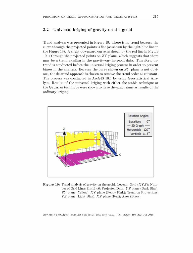
Trend analysis was presented in Figure 19. There is no trend because thecurve through the projected points is flat (as shown by the light blue line inthe Figure 19). A slight downward curve as shown by the red line in Figure19 is through the projected points on ZY plane, which suggests that theremay be a trend existing in the gravity-on-the-geoid data. Therefore, de-trend is conducted before the universal kriging process in order to preventbiases in the analysis. Because the curve shown on ZY plane is not obvi-ous, the de-trend approach is chosen to remove the trend order as constant.The process was conducted in ArcGIS 10.1 by using Geostatistical Ana-lyst. Results of the universal kriging with either the stable technique orthe Gaussian technique were shown to have the exact same as results of theordinary kriging.

Figure 19: Trend analysis of gravity on the geoid. Legend: Grid (XY Z): Num-ber of Grid Lines 11×11×6; Projected Data: Y Z plane (Dark Blue),ZY plane (Yellow), XY plane (Peony Pink); Trend on Projections:Y Z plane (Light Blue), XZ plane (Red); Axes (Black).



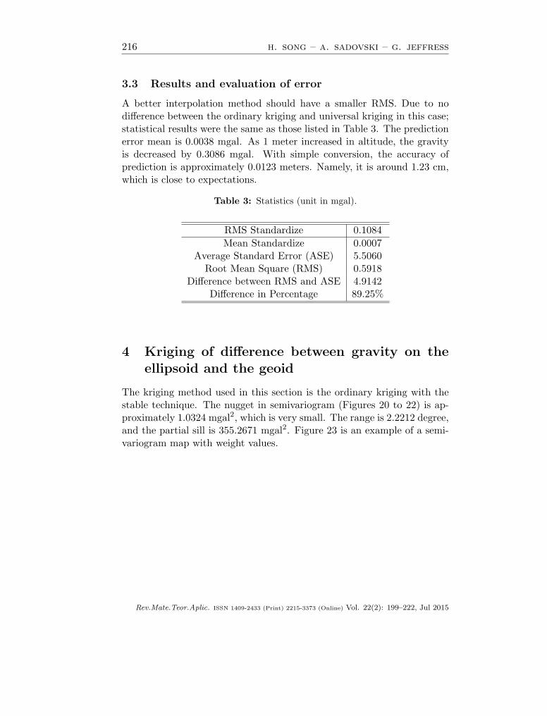
3.3 Results and evaluation of error

A better interpolation method should have a smaller RMS. Due to nodifference between the ordinary kriging and universal kriging in this case;statistical results were the same as those listed in Table 3. The predictionerror mean is 0.0038 mgal. As 1 meter increased in altitude, the gravityis decreased by 0.3086 mgal. With simple conversion, the accuracy ofprediction is approximately 0.0123 meters. Namely, it is around 1.23 cm,which is close to expectations.

Table 3: Statistics (unit in mgal).

RMS Standardize 0.1084

Mean Standardize 0.0007Average Standard Error (ASE) 5.5060

Root Mean Square (RMS) 0.5918Difference between RMS and ASE 4.9142

Difference in Percentage 89.25%

4 Kriging of difference between gravity on theellipsoid and the geoid

The kriging method used in this section is the ordinary kriging with thestable technique. The nugget in semivariogram (Figures 20 to 22) is ap-proximately 1.0324 mgal2, which is very small. The range is 2.2212 degree,and the partial sill is 355.2671 mgal2. Figure 23 is an example of a semi-variogram map with weight values.



Figure 20: Semivariogram model of the ordinary kriging. The averaged semi-variogram values on the y-axis

(in mgal2

), and distance (or lag) on

the x-axis (in degree). Binned values are shown as red dots, whichare sorted the relative values between points based on their distancesand directions and computed a value by square of the difference be-tween the original values of points; Average values are shown asblue crosses, which are generated by binning semivariogram points;The model is shown as blue curve, which is fitted to average values.Model: 1.0324×Nugget+ 355.27× Stable(2.2212, 1.6818).

Figure 21: Semivariogram with all lines (green lines) which fit binned semivar-iogram values. The averaged semivariogram values on the y-axis(in mgal2

), and distance (or lag) on the x-axis (in degree).



Figure 22: Semivariogram with showing search direction. The tolerance is 45and the bandwidth (lags) is 3. The local polynomial shown as agreen line fits the semivariogram surface in this case. The averagedsemivariogram values on the y-axis

(in mgal2

), and distance (or lag)

on the x-axis (in degree).

Figure 23: A semivariogram map. The color band shows semivariogram valueswith weights

(unit in mgal2

).



Figure 24: Cross validation of the ordinary kriging (unit in mgal).

The predicted, error, standard error, and normal QQ plot graphs areplotted respectively in Figure 24 (A to D). Statistical results of the ordi-nary kriging of difference between gravity on the ellipsoid and the geoidlisted in Table 4. The prediction yields very small RMS. The mean ofprediction error is approximately 0.00076 mgal. Figure 25 is the ordinarykriging prediction map which displays the shape of the geoid.

Table 4: Statistics (unit in mgal).

RMS Standardize 0.2249Mean Standardize 0.0007

Average Standard Error (ASE) 1.0672Root Mean Square (RMS) 0.2369

Difference between RMS and ASE 0.8303Difference in Percentage 77.80%



Figure 25: The ordinary kriging predictions map (unit in mgal).



5 Discussion

Geostatistics is a technique that is used to predict unsampled values fromobserved values accurately. Location of attribute values can be referred asthe key of choosing methodology. In this paper, we analyzed four blocksas a group. Thus, a coincident data sample existed in some places. Inthis case, using average of coincident data sample was applied. This mayhave a small influence on the kriging process. In a future study, we willanalyze four blocks individually. In this paper, we have the mean precisionof prediction is around 1.23 cm, which is a very good result for coastalregions.

Acknowledgements

Thanks to NGS at NOAA for open access to download GRAV-D airbornegravity data. For more information and project materials [1, 2, 3, 4, 5],visit NGS on the Web (GRAV-D Homepage: http://www.ngs.noaa.gov/GRAV-D). Other file data used in the map (named as nos80k, state bounds,hydrogp020) was download from USGS [9, 10, 12].

References

[1] Damiani, T.M. (Ed.) (2011) “GRAV-D General Airborne GravityData User Manual”. Theresa M. Diehl, ed., Version 1. GRAV-DScience Team. http://www.ngs.noaa.gov/GRAV-D/data/NGS_

GRAV-D_General_Airborne_Gravity_Data_User_Manual_v1.1.

pdf, accessed 04/19/2012.

[2] GRAV-D Science Team (2011) “Gravity for the Redefinition of theAmerican Vertical Datum (GRAV-D) Project, Airborne GravityData; Block CS01”. In: http://www.ngs.noaa.gov/GRAV-D/data_

cs01.shtml, accessed 04/19/2012.



[4] GRAV-D Science Team (2012) “Gravity for the Redefinition of theAmerican Vertical Datum (GRAV-D) Project, Airborne Gravity



Data; Block CS02”. In: http://www.ngs.noaa.gov/GRAV-D/data_




[6] Hofmann-Wellenhof, B.; Moritz, H. (2006) Physical Geodesy (2nd

ed.). Springer, Wien, New York.

[7] Li, X.; Gotze, H.J. (2001) “Tutorial ellipsoid, geoid, gravity, geodesy,and geophysics”, Geophysics 66(6): 1660–1668.

[8] Moritz, H. (1980) “Geodetic reference system 1980”, Journal ofGeodesy 54(3): 395–405.

[9] National Oceanic and Atmospheric Administration (NOAA); Na-tional Ocean Service (NOS); Office of Coast Survey; Strategic En-vironmental Assessments (SEA); Division of the Office of Ocean Re-sources Conservation and Assessment (ORCA) (1994) “NOS80K -Medium Resolution Digital Vector U.S. Shoreline shapefile for thecontiguous United States”. In: http://coastalmap.marine.usgs.

gov/GISdata/basemaps/coastlines/nos80k/nos80k.zip, accessed01/19/2012.

[10] Paskevich, V. (2005) “STATE BOUNDS: internal US stateboundaries”. In: http://pubs.usgs.gov/of/2005/1071/data/

background/us_bnds/state_bounds.zip, accessed 01/19/2012.

[11] Reguzzoni, M.; Sanso, F.; Venuti, G. (2005) “The theory of generalkriging, with applications to the determination of a local geoid”, Geo-physical Journal International 162(2): 303–314.

[12] U.S. Geological Survey (2003) “HYDROGP020 - U.S. Na-tional Atlas Water Feature Areas: bays, glaciers, lakes andswamps”. In: http://coastalmap.marine.usgs.gov/GISdata/

basemaps/usa/water/hydrogp020.zip, accessed 01/19/2012.


redalyc.precision of geoid approximation and geostatistics ... fileﬁn de establecer gravedad en el...

Documents