ISSN 1178-2293 (Online)

University of Otago Economics Discussion Papers

No. 1014

September 2010

Oil Prices, Exchange Rates and Emerging Stock Markets∗

Syed Abul Basher Department of Research

& Monetary Policy Qatar Central Bank

P.O. Box 1234 Doha, Qatar

bashers@qcb.gov.qa

Alfred A. Haug Department of Economics

University of Otago P.O. Box 56

Dunedin New Zealand

ahaug@business.otago.ac.nz

Perry Sadorsky Schulich School of Business

York University 4700 Keele Street

Toronto, Ontario, Canada M3J 1P3

psadorsk@schulich.yorku.ca

∗ The authors thank, without implicating, Daniel Mitchell and other participants at the WEAI Meeting in Portland (Oregon) for helpful comments.

Abstract

While two different streams of literature exist investigating 1) the relationship between oil prices and emerging market stock prices and 2) oil prices and exchange rates, relatively little is known about the relationship between oil prices, exchange rates and emerging stock markets. This paper proposes and estimates a structural vector autoregression to investigate the dynamic relationship between these variables. Impulse responses are calculated in two ways (standard, projection based methods). The model supports stylized facts. In particular, positive shocks to oil prices tend to depress emerging market stock prices and US dollar exchange rates in the short run. Keywords: Emerging markets; oil prices; exchange rates JEL Classification: G15, Q43

2

1. Introduction

The recent surge in oil prices over the past eight years has generated a lot of interest in

the relationship between oil prices, financial markets and the economy (see, for example,

Blanchard and Gali, 2007, and Herrera and Pesavento, 2009). Crude oil spot prices,

measured using West Texas Intermediate crude oil, closed out the year 2002 at $29.42

per barrel.1 By the June of 2008 spot oil prices had risen to $133.93 per barrel. Over this

same time period, the US dollar fell against other major traded currencies and emerging

market stock prices rose (Figure 1). While there exists a literature on the relationship

between oil prices and stock prices, and a separate literature on the relationship between

oil prices and exchange rates, the relationship between these two streams has, however,

not been that closely studied, especially within the context of emerging market stock

prices. The purpose of this paper is to use a structural vector autoregression (SVAR)

model to bring these two literatures together.

Understanding the relationship between oil prices, exchange rates and emerging stock

market prices is an important topic to study because as emerging economies continue to

grow and prosper, they will exert a larger influence over the global economy. By some

estimates, emerging economies will account for 50% of global GDP by 2050 (Cheng et

al., 2007) and the majority of economic growth. Over the period 1990 to 2005 real GDP

in China and India grew at average annual rates of 7.7% and 7.2% respectively.2 By

comparison, OECD countries grew at an average annual rate of 2.5% over this same

period. At these growth rates the Chinese economy will double every 9 years and the

Indian economy will double every 10 years. Along with this economic growth comes a

voracious demand for energy products such as oil. In 2006, the US was the largest

consumer of oil in the world, accounting for 24% of the global oil demand. China, at 9%

of the world total, had pushed passed Japan to become the second largest oil consuming

nation (Table 1). While the demand for oil in developed economies is holding steady or

declining slightly, the demand for oil in emerging economies is rapidly growing. The

1 http://research.stlouisfed.org/fred2/data/OILPRICE.txt 2 IEA (2007, p.62)

3

International Energy Agency (IEA) (2007, p. 80) predicts that between 2006 and 2030,

China and India will have average annual growth rates in oil of 3.6% and 3.9%

respectively (compared to the 1.3% average annual growth rate for the world). China and

India, combined together will represent 42% of the global increase in oil demand between

2005 and 2030.

Some emerging economies, like China, are accumulating large reserves of foreign

currency (mostly US dollars) and this will make them a bigger player in the world

financial markets. Some estimates place China’s reserves of foreign exchange and gold at

$2.206 trillion as of December 2009.3 Managing this amount of money and protecting its

store of value will mean that China will have not only a greater participation but also a

greater influence over global financial capital markets.

Shocks or unexpected price hikes originating from the oil market have been captured in

different ways.4 Hamilton (2003) defines an oil price shock as a net oil price increase,

which is the log change in the nominal price of oil relative to its previous three year high

if positive, or zero otherwise. However, Kilian (2008a) argues that this measure of oil

price shocks does not necessarily filter out oil price changes due to exogenous political

events or wars because oil price shocks may be demand-driven.5 Furthermore, nominal

oil price shocks do not mean that there are corresponding real oil price shocks. In order

to account for these problems, Kilian (2009) uses a vector autoregression (VAR) with

three variables, the oil supply, the real price of oil and a proxy variable for global demand

for industrial commodities measuring global real economic activity. He identifies, based

on a recursive structure, three oil shocks: an oil supply shock, an oil-market specific

shock and a global demand shock. Kilian (2009) treats these shocks as pre-determined

in secondary ordinary least squares regressions analyzing their effects on the US

economy.6 We model the oil market as in Kilian (2009), however, we use a much less

3 https://www.cia.gov/library/publications/the-world-factbook/rankorder/2188rank.html 4 This literature has been focusing on the US and European economies. 5 See Kilian and Vigfusson (2009) on empirical evidence against such price asymmetries. See also Hamilton (2010). 6 See also Kilian (2008b) for a different definition of oil shocks that are treated as strictly exogenous. These concepts correspond to weak and strong exogeneity in Engle, Hendry and Richard (1983).

4

restrictive set-up for the analysis of the effects of oil shocks that treats all variables as

endogenous and allows for rich dynamics in the interrelations across markets.7

The approach taken in this paper is to use a SVAR to model the dynamic relationship

between real oil prices, an exchange rate index for major currencies, emerging market

stock prices, interest rates, global real economic activity and oil supply. The empirical

results show that the six-variable SVAR model fits the data well in supporting some

stylized facts. Impulse responses are calculated in two alternative ways (standard, local

projection based methods) in order to check their robustness. The results presented in this

paper help to further deepen our understanding of the relationship between oil prices,

exchange rates and emerging markets equity prices.

The rest of the paper is organized as follows. Section 2 discusses the theoretical and

empirical relationship between oil prices, exchange rates and emerging stock prices.

Section 3 describes the data and the identification of the structural VAR model. Section 4

presents the main results of the paper. It also includes the discussion of impulse responses

based on the local projection methods. Some concluding remarks appear in Section 5.

2. Relationships between oil prices, exchange rates and emerging stock markets

Theoretically, oil prices can affect stock prices in several ways. The price of a share in a

company at any point in time is equal to the expected present value of discounted future

cash flows (Huang, Masulis and Stoll, 1996). Oil prices can affect stock prices directly by

impacting future cash flows or indirectly through an impact on the interest rate used to

discount the future cash flows. In the absence of complete substitution effects between

the factors of production, rising oil prices, for example, increase the cost of doing

business and, for non-oil related companies, reduce profits. Rising oil prices can be

passed on to consumers in the form of higher prices for final goods and services, but this

7 We do not require the statistically un-testable assumption of pre-determinedness. Also, our approach does not cause problems with autocorrelated errors and generated regressors (the estimated oil shocks used in secondary regressions) when constructing confidence intervals (Kilian, 2009).

5

will reduce demand for final goods and services and once again reduce profits. Rising oil

prices are often seen as inflationary by policy makers and central banks respond to

inflationary pressures by raising interest rates which affects the discount rate used in the

stock pricing formula.

There is a fairly sizable literature showing that oil price movements affect stock prices

(see, for example, Kaneko and Lee, 1995; Ferson and Harvey, 1994, 1995; Jones and

Kaul, 1996; Huang, Masulis and Stoll, 1996; Sadorsky, 1999; Faff and Brailsford, 1999;

Papapetrou, 2001; Sadorsky, 2001; Hammoudeh and Aleisa, 2004; Hammoudeh,

Dibooglu and Aleisa, 2004; Hammoudeh and Huimin, 2005; El-Sharif, Brown, Burton,

Nixon and Russell, 2005; Huang, Hwang and Peng, 2005; Basher and Sadorsky, 2006;

Boyer and Filion, 2007; Henriques and Sadorsky, 2008; Park and Ratti, 2008).

While most of the research investigating the relationship between oil prices and stock

prices has been conducted using developed economies, there is some research looking

into the relationship between oil prices and emerging stock markets (see for example,

Hammoudeh and Aleisa, 2004; Hammoudeh and Huimin, 2005; Basher and Sadorsky,

2006). On balance, these papers provide evidence that changes in oil prices affect

emerging market stock prices.

Oil price movements are expected to depend upon the demand for oil. While the demand

for oil in most developed economies is growing very slowly or hardly at all, demand for

oil in emerging economies is rapidly increasing. Between 2001 and 2006, for example,

oil consumption has grown the fastest in developing and emerging economies like Qatar,

China, Turkmenistan, United Arab Emirates and Ecuador (Table 1). Over the past ten

years, Qatar, China and Kuwait have each experienced triple digit growth in oil

consumption. China is a particularly interesting country, because in 2006 China’s share

of global oil consumption was 9%, making it the second largest oil consuming country

after the United States. For comparison purposes, the United States is included in Table

1. Notice that for the US, oil consumption growth is actually negative (-1.3%) in the

period 2005-2006. The US is a very important player in the global oil market because it

6

accounts for 24% of global oil consumption, but future growth and pricing pressure is

likely to come from emerging economies. Over the past five years and ten years, the

fastest growing oil consuming region has been the Middle East (Table 2). The second

fastest growing oil consuming region over the past five years and ten years has been Asia

Pacific. Regionally, the demand for oil is growing the fastest in the Middle East, Asia

Pacific and Africa. Emerging market economic and financial activity is likely to be a

factor behind oil price movements. The idea that oil prices respond to strong economic

growth in emerging economies, and especially Asia, has recently been discussed by

Benassy-Quere, Mignon and Penot (2007).

The idea that there is a relationship between oil prices and exchange rates has been

around for some time (early papers, for example, include, Golub, 1983 and Krugman

1983a and b). Bloomberg and Harris (1995) provide a good description, based on the law

of one price, of how exchange rate movements can affect oil prices. Commodities like oil

are fairly homogeneous and internationally traded. The law of one price asserts that as the

US dollar weakens relative to other currencies, ceteris paribus, international buyers of oil

are willing to pay more US dollars for oil. Bloomberg and Harris (1995) find that,

empirically the negative correlation between commodity prices and the US dollar

increased after 1986. In addition to the theoretical and empirical work by Bloomberg and

Harris (1995), empirical papers by Pindyck and Rotemberg (1990) and Sadorsky (2000)

find that changes in exchange rates impact oil prices. Zhang, Fan, Tsai and Wei (2008)

find a significant influence of the US dollar exchange rate on international oil prices in

the long run, but short run effects are limited. Akram (2009) also finds that a weaker

dollar leads to higher commodity prices. Current observations suggest that oil prices and

exchange rates do move together. Figure 1, for example, shows a plot of oil prices

(measured in US dollars) and a trade-weighted US dollar exchange rate (with a higher

value indicating an appreciation of the US dollar while a lower value indicates a

depreciation of the US dollar). From Figure 1, it appears that rising oil prices do coincide

with a weakening of the US dollar.

7

Golub (1983) and Krugman (1983a) put forth compelling arguments as to why

movements in oil prices should affect exchange rates. Golub reasons that since oil prices

are denominated in U.S. dollars, an increase in oil prices will lead to an increase in

demand for U.S. dollars. Golub’s analysis depends upon the crucial assumption that the

demand for oil in oil-importing countries is price inelastic and if the price elasticity is

greater than one (in absolute value) an increase in oil prices will lower total expenditure

on oil and the demand for U.S. dollars would fall. Krugman’s (1983a) analysis is based

on the relationship between the investment portfolio preferences of oil exporters and

movements in exchange rates. Rising oil prices will increase the investment portfolio

possibilities of oil exporters. In Krugman’s (1983a) analysis, exchange rate movements

are determined primarily by current account movements. If rising oil prices lead to a

country’s current account deterioration, then exchange rates will fall.

This discussion on the relationship between oil prices and exchange rates highlights that

there are strong theoretical arguments for why exchange rates should affect oil prices and

there are strong theoretical arguments for why oil prices should affect exchange rates.

Ultimately, the relationship between these two variables can only be resolved through

empirical analysis.

Interest rates may also affect oil prices through a connection with inflation. Unexpected

inflation erodes the real value of investments like stocks and bonds. Central banks can

respond to inflationary pressures by raising interest rates. International investors looking

for better investments in inflationary times may prefer to invest in real assets like oil,

which drives the price of oil up and puts further pressure on inflation. Recycled petro-

dollars from oil rich countries can help to reduce the impact of increases in interest rates

(IEA, 2006, p.39). Akram (2009) finds that commodity prices increase in response to

reductions in real interest rates.

8

3. Model specification

3.1 Choice of variables

For this study, monthly data is collected on global oil production, oil prices, global real

economic activity, exchange rates, emerging market stock prices and interest rates. Our

monthly data cover the sample period from 1988:01 to 2008:12. Following a large body

of research on the significant effect of energy supply disruptions on economic activity,8

oil production variable is included in our model to capture oil supply shock. Following

Kilian (2009), the oil supply shocks are defined as unpredictable innovations to global oil

production. Data on global oil production over the 1987:12—2008:4 period were taken

from Hamilton (2009),9 while the remaining data were updated from the US Energy

Information Department (EIA) database. In the EIA data, global oil supply is defined as

crude oil including lease condensate.

Recent research has documented that oil price reacts differently to oil demand shocks

than oil supply shocks. In particular, Kilian (2009) finds that oil price increases due to

surging global demand produce a less disruptive effect than those caused by losses in

supply. Persistent increase in the (real) price of oil from 2002 to mid-2008 was mainly

driven by strong and increasing global demand for crude oil particularly from India,

China and other emerging countries (Kilian, 2008a; Hamilton, 2009). Therefore, to

account for the effect of global demand on changes of oil price shocks, we have included

a measure of global real economic activity. In so doing, we have followed Kilian (2009)

and use the index of global real economic activity as a proxy for global demand for

industrial commodities. The index is based on dry cargo single voyage ocean freight rates

of different commodities: grain, oilseeds, coal, iron ore, fertilizer and scrap metal. It is

likely to capture shifts in the demand for industrial commodities in global business

8 See Hamilton (2003, 2009) and the references therein. Hamilton (2009) concludes that “historical oil price shocks were primarily caused by significant disruptions in crude oil production that were brought about by largely exogenous geopolitical events.” 9 The global oil production data can be downloaded from James Hamilton’s homepage: http://weber.ucsd.edu/~jhamilto/

9

markets. The detailed construction of the index is described in Kilian (2009). Unlike

OECD indices of industrial production, used in some previous studies on the role of oil,

Kilian’s measure captures recent large increases in global demand for industrial

commodities from emerging countries such as Brazil, China and India. Such a dry goods

measure is more useful for gauging what is happening globally and the movements in

economic and financial activity in emerging economies in particular, where

manufacturing plays an important role. The index is deflated by US consumer price index

(CPI) and is linearly detrended in order to remove the effects of technological advances

in ship-building and other long-term trends in the demand for sea-transport. The

detrended index therefore should capture the cyclical variations in ocean freight rates.

The index is available to download from Lutz Kilian’s homepage.10

Oil prices are measured in dollars per barrel using spot market prices on West Texas

Intermediate crude oil. West Texas Intermediate crude oil is widely seen as a benchmark

for world oil markets. Exchange rates are measured using a trade-weighted exchange rate

index which is a weighted average of the foreign exchange value of the US dollar against

a set of the most widely traded currencies. Globally, there are only a few currencies that

have enough trading volume to affect the foreign exchange markets and oil prices. We

therefore use an exchange rate that captures movements in the most widely traded

currencies. Also, several other currencies not included peg or have pegged their domestic

currency to the US dollar. Higher values of the exchange rate index indicate a stronger

US dollar. Emerging market stock prices are measured using the MSCI emerging stock

market index (measured in US dollars).11 In this paper, the proxy variable for global

interest rate movements is calculated as the difference in the yield spread between the

three month Eurodollar LIBOR (London Interbank Borrowing Rate) and the three month

US Treasury bill rate (the “TED spread”). The yield spread is an interesting variable to

include because movements in the yield curve are often a good predictor of future

10 http://www-personal.umich.edu/~lkilian/ 11 The countries classified as emerging markets changes somewhat from year to year but typically includes the following countries: Brazil, Chile, Colombia, Mexico, Peru, Czech Republic, Egypt, Hungary, Israel, Morocco, Poland, Russia, South Africa, Turkey, China, India, Indonesia, Korea, Malaysia, Philippines, Taiwan and Thailand (http://www.mscibarra.com/products/indices/international_equity_indices/).

10

economic performance. Further, fluctuations in the TED spread may capture fluctuations

in global credit risks (Ferson and Harvey, 1994, 1995).

The data on oil prices, exchange rates and interest rates are available from the Federal

Reserve Bank of St. Louis.12 Stock price data are available from Datastream. Oil prices

and stock prices are converted to real values by deflating by the US CPI. For modeling

purposes, they are expressed in natural logarithms. A dummy variable, which takes on the

value of one from September 1998, is included to capture structural change due to the

Asian financial crises.

3.2 The Structural VAR Model

The empirical model uses global oil production (OILPROD), the logarithm of global real

economic activity (rea), real emerging market stock prices (EMR), real oil prices (OILR),

trade-weighted exchange rates (TWE) and an interest rate spread (TED). Our VAR

model is based on monthly data for oilprod , rea , emr , TED , twe , oilr , where

oilprodt is the logarithm of global crude oil production (OILPROD). The index of real

economic activity is already in logarithms and is denoted reat. The logarithms of the

remaining variables are expressed in small letters. The TWE is an index expressed in

US dollars. The reduced form VAR is given by

∑ , (1)

where c is a vector of constant, p denotes the maximum lag length, Ai are the 6 × 6

parameter coefficient matrices, Dt is a dummy variable to capture the possible effect of

the Asian financial crisis on emerging market stock prices and ut is a vector of error

terms. The structural representation of (1) is given by

∑ , (2)

12 http://research.stlouisfed.org/fred2/; the exchange rate used is denoted TWEXMMTH (1973=100).

11

where εt denotes the vector of structural shocks. Note that the Asian financial crisis

dummy variable does not enter in (2). Denote the total number of variables in the VAR

by K. Assuming B = IK, that is restricting the structural shocks hitting the system to be

mutually uncorrelated innovations with unit variance, now premultiplying (2) with A-1

yields the relationship between the reduced form errors ut and the structural shocks εt as13

. (3)

After normalizing the K diagonal elements of A to 1’s, an exact identification of the

structural equation requires imposing K(K-1)/2 restrictions on A. We employ only short-

run restrictions on contemporaneous relations and no long-run restrictions. Moreover, we

do not impose any restrictions on the lagged coefficients in equation (2). The short-run

restrictions impose some contemporaneous feedback effects among the variables in the

model. Christiano, Eichenbaum and Vigfusson (2007) argue that structural VARs based

on short-run restrictions perform “reasonably well”. Since we do not attempt to test any

particular model, we base our identification restrictions on different economic models as

well as economic ad-hoc reasoning.

3.3 Identification of Structural Shocks

The identification procedure for equation (3) is given as

0 0 0 0 00 0 0 0 000 0 00 0

0 0 0

(4)

The restrictions on may be motivated as follows. The identifying restriction in the

equations for oil supply and global demand takes these two variables as being

13 See e.g. Hamilton (1994, Ch. 11) for further details.

12

contemporaneously exogenous to the other variables in the system. We have thus

assumed that both oil supply and global (oil) demand, due to real economic activity, do

not contemporaneously react to shocks to other variables in the system within a month.

These exclusion restrictions seem quite plausible since it is very unlikely for, say, Saudi

Arabia to react immediately within the same month with a change to its crude production

level following, for example, an oil price or an exchange rate shock. Likewise, it is quite

probable that there might be a significant time delay before consumers and businesses

revise their consumption plans following a shock. Needless to say, lagged values of oil

supply and global demand are allowed to react to macroeconomic shocks after the first

month has passed.14

Following the discussion in Section 2, emerging market equity prices are allowed to

contemporaneously react to interest rate, exchange rate and oil price shocks, besides

reacting to aggregate demand shocks. Unlike the long delay in adjustments in the goods

sectors, financial markets react swiftly to changes in macroeconomic news. For example,

energy based equities will react instantaneously to a positive change in the oil price,

while a dollar appreciation effectively makes emerging equities less competitive than

dollar-denominated assets. In the fourth equation, the interest rate spread is allowed to

react contemporaneously to a global demand shock and an oil price shock, with the

former predicted to generate a positive impact on interest rates while the latter is

presumably inversely related to interest rates.

Changes in global demand, emerging market equity prices and oil prices result in a

contemporaneous change in the trade-weighted US dollar index. Since oil is denominated

in dollars, in the face of a declining dollar, with the relative price of oil being set in

equilibrium, the dollar price of oil must rise instantaneously. Figure 1, which depicts the

time series of the real oil price and the trade-weighted value of the dollar (along with the

remaining model’s variables), does seem to lend support to this idea, especially since the

start of 2002. Relative strength in global demand is also likely to impact the US dollar

14 Crude oil price shocks affect shipping freight rates because bunker fuel oil is an input to shipping services. However, following Kilian (2009), we assume that the effect occurs with a delay and not within the same month. Kilian (2009) found no contemporaneous correlation between the two time series.

13

within the same month because of the dollar’s role as the dominant invoicing currency in

international trade (see, Goldberg and Tille, 2008). In the sixth and final equation we

assume that changes in global oil production and global aggregate demand

contemporaneously affect real oil prices.

4. Empirical results

This section is divided into three parts. First, we present preliminary results on the time

series properties of our data. Second, we present the main results of the paper, the

restricted structural VAR analysis for the model discussed in Section 3.3. Third, we

study the robustness of the impulse response analysis by employing local projection

instead of standard methods.

4.1 Preliminary results

4.1.1 Graphical analysis

Figure 1 shows a plot of global oil production (OILPROD), the logarithm of real global

economic activity (rea), emerging market stock prices (EM), the TED spread, exchange

rates (TWE) and oil prices (OIL). Each variable is expressed in nominal terms, except

when noted otherwise. Notice how closely oil prices and emerging market stock prices

track each other. Both tend to rise and fall often at the same time. Also notice that

exchange rates and oil prices tend, for the most part, to move in opposite directions. A

lower US dollar coincides with higher oil prices and vice versa.

4.1.2 Descriptive statistics

Table 3 presents some summary statistics of the model’s variables. Some remarks are in

order. The average oil price during the sample period is about $32.50, with a maximum

of nearly $134 observed during mid-2008. A 5.863% decline in the rate of change of

global oil production took place in August 1990, as a result of the Iraqi invasion of

Kuwait (the first Gulf war). Interestingly, this decline is immediately compensated by a

4.473% increase in global oil production in the following month (September 1990). The

14

yield spread between the 3-month Eurodollar LIBOR and the 3-month US T-bill (the

TED spread) was generally higher during the end of the sample, reflecting the effect of

the 2007-08 global financial crisis. For example, a 4.620 spread was observed in October

2008, a month after the collapse of Lehman Brothers, which is extremely large by

comparison to the pre-2007 period. The coefficient of variation, a normalized measure of

dispersion, which is defined as the ratio of the standard deviation to the mean, portrays

highest variability for real global activity followed by the percentage change in global oil

supply and the TED spread. The US dollar exchange rate index (TWE) has the least

variability compared with other variables. Further, the skewness and kurtosis statistic for

the dollar index is very close to normality, which is further supported by the Jarque-Bera

test statistic, suggesting that the null hypothesis of normality is not rejected for the

exchange rate, while the null of normality is strongly rejected for the remaining

variables.15

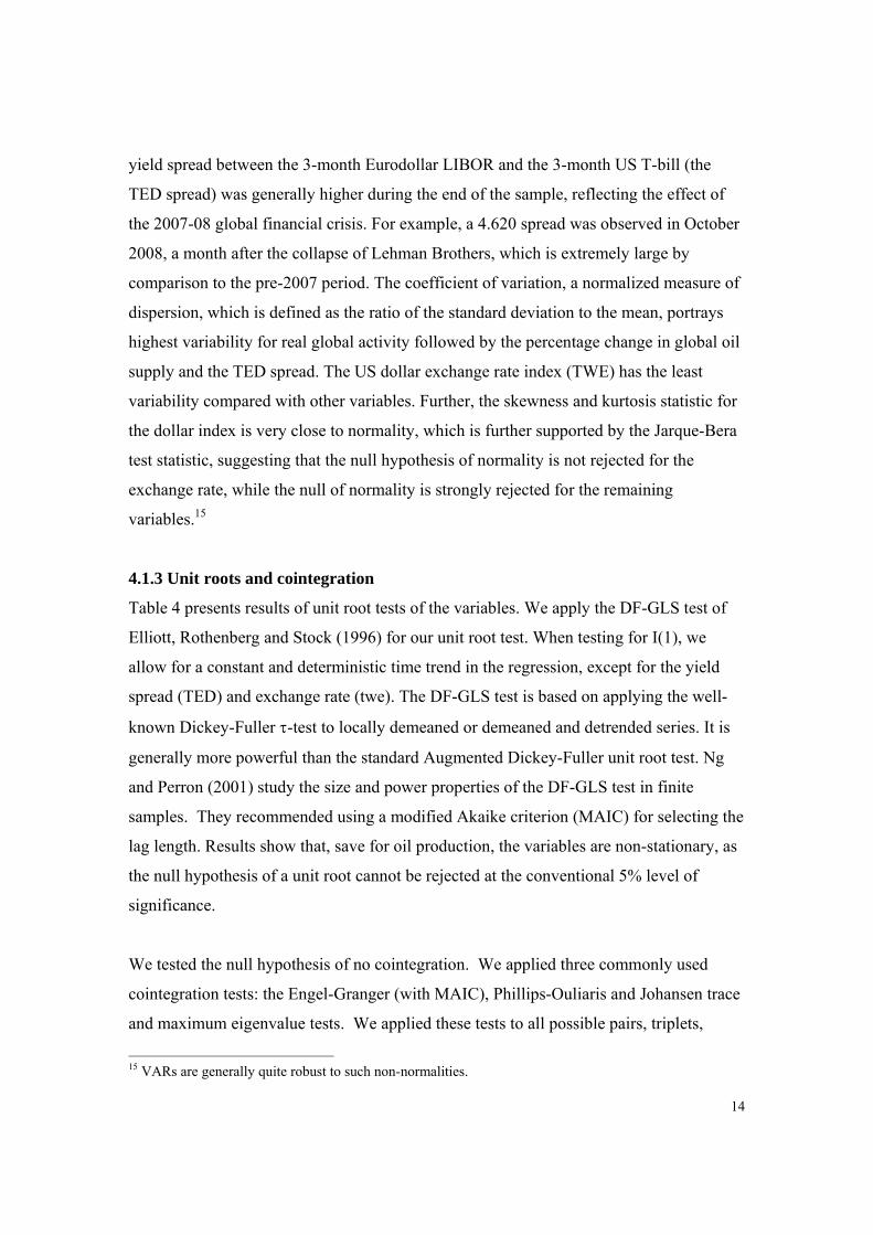
4.1.3 Unit roots and cointegration

Table 4 presents results of unit root tests of the variables. We apply the DF-GLS test of

Elliott, Rothenberg and Stock (1996) for our unit root test. When testing for I(1), we

allow for a constant and deterministic time trend in the regression, except for the yield

spread (TED) and exchange rate (twe). The DF-GLS test is based on applying the well-

known Dickey-Fuller τ-test to locally demeaned or demeaned and detrended series. It is

generally more powerful than the standard Augmented Dickey-Fuller unit root test. Ng

and Perron (2001) study the size and power properties of the DF-GLS test in finite

samples. They recommended using a modified Akaike criterion (MAIC) for selecting the

lag length. Results show that, save for oil production, the variables are non-stationary, as

the null hypothesis of a unit root cannot be rejected at the conventional 5% level of

significance.

We tested the null hypothesis of no cointegration. We applied three commonly used

cointegration tests: the Engel-Granger (with MAIC), Phillips-Ouliaris and Johansen trace

and maximum eigenvalue tests. We applied these tests to all possible pairs, triplets,

15 VARs are generally quite robust to such non-normalities.

15

quadruplets and quintuplets of variables and also to the six variables together. We found

rather mixed evidence (not reported) depending on the test used, whether or not a linear

time trend is considered, and on the lag selection method used. The VAR with all six

variables shows two cointegrating vector with the trace test, however, only one with the

maximum eigenvalue test, at the usual 5% significance level. Our conflicting evidence

here is consistent with the findings of Gregory, Haug and Lomuto (2004) for Monte

Carlo simulations and for a comparison of alternative cointegration tests applied to 132

data sets from 34 studies.

The finding of unit roots in variables raises the question whether to estimate the structural

VAR in levels (i.e., with variables in non-stationary form), first-differenced (i.e., with

variables in stationary form) or in a VAR that imposes cointegration (i.e., in an error-

correction model). A considerable literature on this issue tends to suggest that even if the

variables have unit roots, it is still desirable to estimate a structural VAR in level. Sims,

Stock and Watson (1990) show that the estimated coefficients of a VAR are consistent

and the asymptotic distribution of individual estimated parameters is standard (i.e., the

asymptotic normal distribution applies) when variables have unit roots and there are some

variables that form a cointegrating relationship.16 We do not impose possible unit roots

and cointegration in our VAR. We justify the specification in levels based on the Monte

Carlo results of Lin and Tsay (1996). The problem is that cointegration tests often

indicate too many, or occasionally too few, cointegrating vectors and therefore lead to

misspecification. On the other hand, a VAR specified in first differences assumes that

variables are not cointegrated because no error-correction terms are included. If there is

cointegration, then such a model in first differences is misspecified. The impulse

response functions of the VAR model in levels are also consistent estimators of their true

impulse response functions both in the short- and medium-run, except in the longer-run.

As shown by Phillips (1998), in the longer-run the standard impulse responses do not

converge to their true values with a probability of one when unit roots or near-unit roots

are present and the lead time of the impulse response function is a fixed fraction of the

sample size. For this reason, we apply an alternative method for estimating the impulse

16 See also Hamilton (1994, pp. 561-562) for a related discussion.

16

responses based on local linear projections suggested by Jordà (2005) that is robust to this

problem.

4.2 The main SVAR model

The VAR consists of the six variables as defined previously: oilprodt , reat , emrt , TEDt ,

twet and oilrt. The VAR lag length p is set at 9. With this lag length, the residuals are

randomly distributed and the VAR has stable roots. The identification system is given by

(4).

Figure 2 displays the response of global oil production, real economic activity, equity

prices, interest rates, exchange rates and oil prices to a one-standard deviation structural

innovation. The two-standard-error confidence intervals are shown by short-dashed lines.

Our discussion of the impulse response functions (IRFs) mainly centers on the responses

of oil supply, emerging equity prices, exchange rate, and oil prices to their own and other

shocks, which is the main interest of the paper. Given oil production shocks and global

demand shocks, as captured by global real economic activity shocks, are treated as

contemporaneously exogenous to the other variables in the system, it is interesting to

analyze how the two variables react to their own shock. As can be seen from Figure 2, a

positive oil supply shock causes a statistically significant increase in global oil production

that is sustained over the entire 24-month period considered in the graph.17 This possibly

reflects the discovery of new oil fields, better extraction technologies or a decline in

OPEC’s control over the oil supply. By comparison, a positive global demand shock

stimulates real economic activity in the first few months after the impact and then slowly

winds down in a persistent fashion. It becomes statistically insignificantly different from

zero after about 15 months, reflecting typical short-run macroeconomic multiplier effects

over the business cycle from aggregate demand stimulation.18 A positive oil supply

17 Kilian (2009), among others, use the percentage change in oil production instead of the log levels. We tried this measure but found no significant changes in the IRF graphs. In principal, one should treat all variables the same so that a log-levels specification for oil production would seem preferable. Also, the two-standard-error confidence bands in our graphs are roughly equal to 95% confidence bands. 18Unanticipated demand expansion also leads to a sustained increase in oil production and in oil prices because of the associated increase in real economic activity. However, these effects are somewhat

17

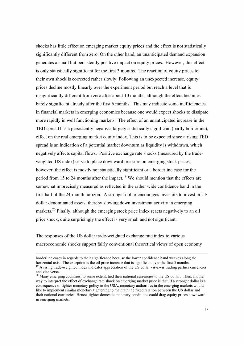
shocks has little effect on emerging market equity prices and the effect is not statistically

significantly different from zero. On the other hand, an unanticipated demand expansion

generates a small but persistently positive impact on equity prices. However, this effect

is only statistically significant for the first 3 months. The reaction of equity prices to

their own shock is corrected rather slowly. Following an unexpected increase, equity

prices decline mostly linearly over the experiment period but reach a level that is

insignificantly different from zero after about 10 months, although the effect becomes

barely significant already after the first 6 months. This may indicate some inefficiencies

in financial markets in emerging economies because one would expect shocks to dissipate

more rapidly in well functioning markets. The effect of an unanticipated increase in the

TED spread has a persistently negative, largely statistically significant (partly borderline),

effect on the real emerging market equity index. This is to be expected since a rising TED

spread is an indication of a potential market downturn as liquidity is withdrawn, which

negatively affects capital flows. Positive exchange rate shocks (measured by the trade-

weighted US index) serve to place downward pressure on emerging stock prices,

however, the effect is mostly not statistically significant or a borderline case for the

period from 15 to 24 months after the impact.19 We should mention that the effects are

somewhat imprecisely measured as reflected in the rather wide confidence band in the

first half of the 24-month horizon. A stronger dollar encourages investors to invest in US

dollar denominated assets, thereby slowing down investment activity in emerging

markets.20 Finally, although the emerging stock price index reacts negatively to an oil

price shock, quite surprisingly the effect is very small and not significant.

The responses of the US dollar trade-weighted exchange rate index to various

macroeconomic shocks support fairly conventional theoretical views of open economy

borderline cases in regards to their significance because the lower confidence band weaves along the horizontal axis. The exception is the oil price increase that is significant over the first 5 months. 19 A rising trade-weighted index indicates appreciation of the US dollar vis-à-vis trading partner currencies, and vice versa. 20 Many emerging countries, to some extent, tied their national currencies to the US dollar. Thus, another way to interpret the effect of exchange rate shock on emerging market price is that, if a stronger dollar is a consequence of tighter monetary policy in the USA, monetary authorities in the emerging markets would like to implement similar monetary tightening to maintain the fixed relation between the US dollar and their national currencies. Hence, tighter domestic monetary conditions could drag equity prices downward in emerging markets.

18

macroeconomics. Global oil supply shocks appear to have no visible effect on the

exchange rate, judging by the nearly horizontal impulse function and its statistical

insignificance. On the contrary, an unanticipated global demand expansion produces a

lasting downward impact on the US dollar (i.e. depreciation), though it shows borderline

significance. This seems to suggest that the source of the global demand buoyancy is not

US originated. Indeed, the collapse of the US dollar over the 2002-2008 period combined

with the simultaneous expansion of many emerging economies (e.g. Brazil, China and

India) appears to be consistent with this evidence. The response of the US dollar index to

an emerging market equity price shock is very small and clearly insignificant. A positive

TED spread shock slightly raises at first and then lowers the US dollar index over the first

10 months and then increases it afterwards. Whilst all these effects are not significantly

different from zero, except for the first 2 months, the eventual appreciation of the US

dollar is likely a reflection of investors’ deleveraging activity where a lasting rise in the

TED spread leads investors to rush away from risky assets and favor dollar-denominated

assets.21 The exchange rate initially slightly rises after the impact to its own shock and

thereafter pretty much stays at the elevated level, indicating a permanent effect of the

shock. The initial US dollar response to a positive oil price shock is negative, reflecting

the numeraire effect as oil is priced in US dollar. However, these effects are small and

only (barely) significant for the first 2-3 months. This result is consistent with Krugman’s

(1983a) analysis that exchange rate movements are determined primarily by current

account movements. In the case of a large net importer of oil like the United States, rising

oil prices lead to a current account deterioration and then exchange rates will fall.

The reaction of the oil price to a positive oil production shock is negative for the first 4

months, as one would expect; effects thereafter are no longer statistically significant. A

positive global demand shock increases the oil price further after the impact for about 3

months, thereafter it begins to fall and becomes insignificantly different from zero in 5

months after the impact. By contrast, the oil price displays a positive hump-shaped 21 When the crisis intensified after the bankruptcy of Lehman Brothers, private foreign investors lowered the risk in their portfolios by turning to US Treasury securities. The global flight to safety into US Treasury bills during the recent financial crisis had in turn strengthened the US dollar (see, McCauley and McGuire, 2009). See also Melvin and Taylor (2009) for the implications of the deleveraging in financial markets on foreign exchange markets during the recent financial crisis.

19

response to a positive equity shock but the effect is mostly not significant, except for the

5-10 month period after the impact, where it is of borderline statistical significance. A

positive TED spread shock leads to a fall in oil prices after the impact for the first 2-3

months, followed by a quick reversal—all occurring within the first 6-7 months—

thereafter the effects fade into insignificance. Unanticipated exchange rate increases

lower oil prices but the impact is not significant, except possibly after a 15 month delay.

Finally, oil prices increase after an oil price shock for 2-3 months and then fall but

eventually stay at a level higher than before the shock. These effects are though

statistically significant only for the first 6 months after the impact.

The results from our six-variable SVAR can be compared to the results for the oil market

in Kilian’s (2009) three-variable VAR with recursive identification. The data sets for the

oil-market variables are not identical because we use updated data. The

contemporaneous identification scheme for the three variables in our SVAR is almost

identical, except that we set equal to zero so that aggregate demand does not respond

contemporaneously to an oil price shock, however, we explore in Section 4.3.2 whether

this restriction affects results. An oil supply shock (positive in our case) has very much

the same effects on global oil production and on real oil prices as in Kilian (2009). It

leads to a sharp increase in global oil production on impact, followed by a partial reversal

within the first 8 month and then a slight increase that is sustained. However, an

aggregate demand shock shows a somewhat different profile. It is persistent and highly

significant as in Kilian (2009), but in our case the effect starts to decline already after 3-4

months instead of after 14 months in Kilian, and becomes insignificant after 15 months in

our case. It also increase oil production persistently and oil prices, especially for the first

2-3 months after the impact, with a reversal thereafter before leveling off at a

permanently higher level, being a borderline case with respect to significance after 5

months. In Kilian (2009) the increase is delayed by 6 months and is significant over the

entire 20 months considered in his graph. A positive oil price shock, interpreted by

Kilian (2009) as shock due to a precautionary oil demand shock, shows pretty much the

same profile over time in both analyses.22 The effects on real economic activity and oil

22 Hamilton (2009) questions the interpretation of these price shocks as precautionary demand shocks.

20

production are not significant in our case, whereas Kilian (2009) found a positive but

small effect on real economic activity.

4.3 Robustness of the impulse responses

4.3.1 Different estimation method: Local projection based impulse responses

The preceding impulse response functions were derived with standard impulse response

function analysis. The standard method is based on a moving average representation of

the VAR model. The VAR is estimated first and then a vector moving-average (VMA) is

formed in order to derive the effects of experimental shocks on the variables over time.

The impulse responses are derived iteratively, moving forward period-by-period, relying

on the same set of original VAR parameter estimates each time. There are several

problems with the standard approach to impulse response analysis. These problems are

magnified by the iterative process.

First, the true and generally unknown data-generating process of the economic model

may be poorly approximated by a VAR, even with relatively long lag structures.23 The

reason is that moving average components in the data may not be captured adequately by

the VAR. Second, VMA representations of the VAR may not be unique and different

invertibility assumptions can lead to vastly different impulse responses.24 Third, unit or

near-unit roots and cointegration in the VAR can lead to inconsistent impulse responses

at longer horizons when the lead time of the impulse response function is a fixed fraction

of the sample size (Phillips, 1998; Pesavento and Rossi, 2006). These problems open

various possibilities for misspecification of the VAR that might be relatively small.

However, the highly non-linear transformations used in the derivation of standard

impulse responses will amplify the effects of misspecifications and lead to unreliable

impulse response functions.

23 See, Kapetanios, Pagan and Scott (2007), among others. 24 See, Hansen and Sargent (1980), Frenández-Villaverde et al. (2007) and Sims (2009).

21

Jordà (2005) has proposed an alternative approach for deriving impulse response

functions. Instead of non-linear transformations, local linear projections are applied in

order to obtain impulse responses. An impulse response can be regarded as a revision in

the forecast of a variable at a future horizon t+s to a one-time experimental shock at time

t. Jordà (2005) applies multi-step direct forecast for every horizon. The forecast or

projection is local to the horizon, or put differently, a separate forecasting regression is

run for every horizon. Jordà (2005) proves that impulse responses based on direct

forecasts are consistent and asymptotically normal. Furthermore, he demonstrates in

Monte Carlo simulations that local linear projections estimate impulse responses more

accurately than standard methods, especially at medium to longer horizons. Also, the loss

of efficiency from using local projection impulse responses (instead of a correctly

specified VAR) appears to be very small. Local projection based impulse responses are

more robust to misspecification than standard ones.

Jordà’s (2005) local projection based impulses use a recursive causal ordering for

structural shocks, which cannot be compared with the non-recursive identification

schemes discussed in the previous section. Recently, Haug and Smith (2007) have

extended Jordà’s (2005) method to a non-recursive identification scheme, which is

appropriate for our purpose. Briefly, Jordà’s (2005) method can be summarized as

follows. Consider an n-dimensional vector of random variables. Following Jordà

(2005), we define the impulse response (IR) at time t+s arising from the ith experimental

shocks at time t as:

, , | ; | ; ,

where 0,1,2, … , ; 0,1,2, … ; , , … ; is a vector additively

conformable to ; and 0 is a vector of zeroes. The expectations are formed by linearly

projecting onto the space of :

… ,

where is a vector of constants and the are coefficient matrices at lag j and

horizon s+1. For every horizon 0,1,2, … , , a projection or forecast regression is done

in order to estimate the coefficients in . The estimated IRF is then given by:

, ,

22

with the normalization , the identity matrix. Thus, an innovation or impulse to the

ith variable in the vector , denote , produces an impulse response of . The

horizon of the forecast is s and | ; shows the forecast after a shock in period t.

The impulse responses from local approximations can be calculated from univariate least

squares regressions for each variable at every horizon. Jordà’s (2005) demonstrates that

inference can be performed with standard heteroscedastic and autocorrelation (HAC)

robust standard errors, such as Newey-West standard errors that we apply. These HAC

standard errors correct for the moving average terms that exist in forecast errors.

Figure 3 shows projection based impulse responses for the SVAR system with two

standard error confidence bands and Figure 4 reports results for one standard error

confidence band, as is common in the literature (e.g., Kilian, 2009). With some

exceptions, we can see that the projection based IRFs (indicated by dashed blue lines)

generally follow a pattern remarkably similar to that of VMA-based IRFs (indicated by

the solid black line). One notable difference is that the local-projection IRFs show a less

pronounced cyclical response of the TED in response to a real economic activity shock

and to its own shock in particular, compared to the standard IRFs. Most importantly, the

response of equity prices to an oil price shock is statistically significant for projection

based IRFs for the first 3 months in Figure 3 and for the first 4 months in Figure 4.

Furthermore, a positive oil price shock now also leads to an immediate drop in the

exchange rate that is statistically significant for the first 2-3 months after the impact in

Figure 3 and the first 3-4 months in Figure 4. Aside from this, there are only small

differences in the overall evolvement of the IRF graphs over time. Further, confidence

bands have similar coverage, with a few initial responses becoming less significant.

Overall, the IRFs show considerable robustness with respect to the two different

estimation methods. This demonstrates the reliability of our model as specified.

23

4.3.2 Different identification schemes

We consider two modified identification schemes to our baseline model given in equation

(4).25 We do not provide graphs in order to conserve space, but they are available on

request from the authors. The first scheme does not restrict to be equal to zero. This

is motivated by Kilian’s (2009) recursive (Choleski) scheme for his three-variable oil-

market VAR that does not allow him setting to zero. It means that we allow for the

possibility that global aggregate demand responds to an oil supply shock within the same

month. In other words, oil supply shocks have immediate effects. This change has no

noticeable effect on all our IRFs reported in Figure 2, consistent with our assumption in

the baseline identification scheme that oil supply (production of crude oil) shocks

stimulate or depress aggregate demand with a delay.

The second identification scheme restricts to equal zero, i.e. the exchange rate does

not respond contemporaneously to an oil price shock. We expect this to be an unrealistic

assumption because foreign exchange markets are efficient markets. Unless oil price

shocks are perceived in this market as irrelevant, we expect to see changes in the IRFs.

Indeed, this change affects four IRF graphs in a significant way. A positive exchange

rate shock has now a long lasting and significant effect on the emerging stock market for

about a year, even though the exchange rate itself is not reacting in any significant way to

its own shock. Similarly, an emerging stock market shock has no significant effects on

the stock market but seems to affect negatively the exchange rate in a significant and

permanent way. Therefore, our baseline identification scheme that does not restrict

to equal zero seems more reasonable.

5. Conclusions

Recognizing the importance of the relationship between stock prices and oil prices and

the relationship between oil prices and exchange rates, this paper combines these two

streams of literature together into one empirical structural vector autoregression model. In

25 We tried other identification schemes for the contemporaneous relations but either could not estimate the matrix A-1 because of non-convergence or the IRF results did not make economic sense.

24

doing so, it is possible to gain a more complete understanding of the relationship between

oil prices, emerging market stock prices and exchange rates. This is important to do so

because emerging economies have, over the past ten year, been accounting for a larger

proportion of global GDP and this trend is expected to continue. Emerging economies are

among the fastest growing economies (with GDP growth rates much faster than the

growth rates observed in developed economies) and this combination of size and growth

is likely to influence the dynamics between oil prices, emerging market stock prices and

exchange rates.

The short term dynamics between oil prices, emerging market stock prices and exchange

rates are analyzed using two sets of impulse response functions (standard, local

projection based). In most cases the projection based IRFs provide similar results as the

standard IRFs. Where the two approaches differ, the projection based approach tends to

provide impulse responses that are more likely to adequately capture the cyclical

response of a variable to an unexpected structural shock. Both approaches for example

report that stock prices respond negatively to a positive oil price shock, and that oil prices

respond positively to a positive emerging market shock. However, the first effect is only

statistically significant for the projection based impulses for the first 3-4 months after the

impact. The second effect is barely statistically significant in the period 5-10 months

after the impact for standard impulses and is statistically significant in that period for

projection based responses with one standard error confidence bands. These results

indicate that while increases in oil prices depress stock prices (a result widely supported

by the literature documenting the effects of oil prices on stock markets) it is also the case

that increases in emerging market stock markets lead to an increase in oil prices. This

latter result makes sense within the context of global oil markets and global economic

activity. Oil consumption in most developed economies is flat or in decline and as a result

emerging market economic growth (as proxied by emerging market stock prices) is likely

to be an important source of demand side pricing pressure in the oil market.

The results in this paper support to some extent that oil prices respond to movements in

exchange rates. Further, the results reported in this paper offer some support for higher

25

oil prices affecting exchange rates in the short run. In particular, a positive oil price shock

leads to an immediate drop in the trade-weighted exchange rate. This result has a

statistically significant impact for about 3 months.

The results in this paper show that oil prices respond negatively to an unexpected

increase in oil supply and oil prices respond positively to an unexpected increase in

demand. These results are consistent with the predictions from a demand and supply

model for the oil market. Oil prices respond positively to a positive shock to emerging

stock markets, while oil prices respond negatively to a positive shock to the TED spread.

These results are important in establishing, that in addition to global supply and demand

conditions for oil, oil prices also respond to emerging market equity markets and global

financial capital markets.

The results in this paper have a number of policy implications. As expected, oil prices

respond to global oil production (supply) and real global economic activity (demand).

Rapidly rising stock prices in emerging economies or an increased demand for global

credit are two factors which can also put pressure on oil prices to rise. While it has

typically been the case that macroeconomic policy in developed economies, like the G7,

was seen as an important factor affecting the global economy, it now must be recognized

that monetary and fiscal policy in large emerging economies (like China and India) can

affect their own economic growth prospects as well as global financial markets. As the

results in this paper have shown, oil prices respond not just to economic fundamentals

like oil supply and real economic activity but also to movements in emerging stock prices

and the TED spread. Stock markets are often seen as leading economic indicators.

Rapidly rising stock prices in emerging markets signals the expectation of higher

economic growth ahead. If emerging market stock prices get trapped in a bubble,

however, oil prices will overshoot in relation to economic fundamentals. This means that

consumers in developed economies could end up paying more for oil and oil related

products even if their own domestic economic growth remains sluggish and future

realized economic growth in emerging economies is less than what the financial markets

expected.

26

References

Akram, Q.F. 2009. Commodity prices, interest rates and the dollar, Energy Economics, 31, 838-851. Basher, S.A. and Sadorsky, P. 2006. Oil price risk and emerging stock markets, Global Finance Journal, 17, 224-251. Benassy-Quere, A., Mignon, V. and Penot, A. 2007. China and the relationship between the oil price and the dollar, Energy Policy, 35, 5795-5805. Blanchard, O, and Gali, J. 2007. The macroeconomic effects of oil shocks: Why are the 2000s so different from the 1970s? NBER Working Paper 13368, National Bureau of Economic Research. Bloomberg, S.B. and Harris, E.S. 1995. The commodity-consumer price connection: Fact or fable? Federal Reserve Board of New York, Economic Policy Review, October, 21-38. Boyer, M.M. and Filion, D. 2007. Common and fundamental factors in stock returns of Canadian oil and gas companies, Energy Economics, 29, 428-453. BP Statistical Review of World Energy, June 2007 (www.BP.com). Cheng, H-F,Gutierrez, M.,Mahajan, A.,Shachmurove, Y. and Shahrokhi, M. 2007. A future global economy to be built by BRICs, Global Finance Journal, 18, 143-156. Christiano, L., Eichenbaum, M. and R. Vigfusson (2007). Assessing structural VARs: in D. Acemoglu, K. Rogoff, and M. Woodford (eds.), NBER Macroeconomics Annual, Volume 21, National Bureau of Economic Research, MIT–Press. Elliott, G., Rothenberg. T. J. and Stock, J. H. 1996. Efficient tests for an autoregressive unit root, Econometrica, 64, 813-836. El-Sharif, I., Brown, D., Burton, B., Nixon, B. and Russell, A. 2005. Evidence on the nature and extent of the relationship between oil prices and equity values in the UK, Energy Economics, 27, 819-830. Engle, R. F., Hendry, D.F. and Richard, J.-F. (1983). Exogeneity, Econometrica, 51, 277–304. Faff, R.W. and Brailsford, T.J. 1999. Oil price risk and the Australian stock market, Journal of Energy Finance and Development, 4, 69-87. Fernández-Villaverde, J., Rubio-Ramírez, J.F., Sargent, T.J. and Watson, M.W. 2007. ABCs (and Ds) of understanding VARs, American Economic Review, 97, 1021-1026.

27

Ferson, W.W. and Harvey, C.R. 1994. Sources of risk and expected returns in global equity markets, Journal of Banking and Finance, 18, 775-803. Ferson, W.W. and Harvey, C.R. 1995. Predictability and time-varying risk in world equity markets, Research in Finance, 13, 25-88. Goldberg, L. and Tille, C. 2008. Vehicle currency use in international trade, Journal of International Economics, 76, 177-192. Golub, S. 1983. Oil prices and exchange rates, Economic Journal, 93, 576-593. Gregory, A.W., Haug, A.A. and Lomuto, N. 2004. Mixed signals among tests for cointegration, Journal of Applied Econometrics, 19, 89-98. Hamilton, J.D. 1994. Time Series Analysis, Princeton, NJ: Princeton University Press. Hamilton, J.D. 2003. What is an oil shock? Journal of Econometrics, 113, 363-398. Hamilton, J.D. 2009. Causes and consequences of the oil shock of 2007-08, Brookings Papers on Economics Activity, Spring, 215-259. Hamilton, J.D. 2010. Nonlinearities and the macroeconomic effects of oil prices, NBER Working Paper No. 16186. Hammoudeh, S. and Aleisa, E. 2004. Dynamic relationships among GCC stock markets and NYMEX oil futures, Contemporary Economic Policy, 22, 250-269. Hammoudeh, S., Dibooglu, S. and Aleisa, E. 2004. Relationships among US oil prices and oil industry equity indices, International Review of Economics and Finance, 13, 427-453. Hammoudeh, S. and Huimin, L. 2005, Oil sensitivity and systematic risk in oil-sensitive stock indices, Journal of Economics and Business, 57, 1-21. Hansen, L. P. and Sargent, T.J. 1980. Formulating and estimating linear rational expectations models, Journal of Economic Dynamics and Control, 2, 7–46. Haug, A. and Smith, C. 2007. Local linear impulse responses for a small open economy, Reserve Bank of New Zealand Discussion Paper DP2007/09, available at http://www.rbnz.govt.nz/research/discusspapers/dp07_09.pdf Henriques, I. and Sadorsky, P. 2008. Oil prices and the stock prices of alternative energy companies, Energy Economics, 30, 998-1010. Herrera, A.M. and Pesavento, E. 2009. Oil price shocks, systematic monetary policy, and the ‘Great Moderation’, Macroeconomic Dynamics, 13, 107-137.

28

Huang, R. D., Masulis, R.W. and Stoll, H.R. 1996. Energy shocks and financial markets, Journal of Futures Markets, 16, 1-27. Huang, B.-N., Hwang, M.J. and Peng, H-P. 2005. The asymmetry of the impact of oil price shocks on economic activities: An application of the multivariate threshold model, Energy Economics, 27, 455-476. International Energy Agency. 2006. World Energy Outlook, Paris. International Energy Agency. 2007. World Energy Outlook, Paris. Jones, C. and Kaul, G. 1996. Oil and the stock markets, Journal of Finance, 51, 463-91. Jordà, O. 2005. Estimation and inference of impulse responses by local projections, American Economic Review, 95, 161–182. Kaneko, T. and Lee, B.S. 1995. Relative importance of economic factors in the US and Japanese stock markets, Journal of the Japanese and International Economies, 9, 290-307. Kapetanios, G., Pagan, A. and Scott, A. 2007. Making a match: Combining theory and evidence in policy-oriented macroeconomic modelling, Journal of Econometrics, 136, 565–594. Kilian, L., 2008a. Exogenous oil supply shocks: How big are they and how much do they matter for the US economy? Review of Economics and Statistics, 90, 216–240. Kilian, L., 2008b. A comparison of the effects of exogenous oil supply shocks on output and inflation in the G-7 countries, Journal of the European Economic Association, 6, 78-121. Kilian, L., 2009. Not all oil price shocks are alike: disentangling demand and supply shocks in the crude oil market, American Economic Review, 99, 1053-1069. Kilian, L. and Vigfusson, R.J. 2009. Pitfalls in estimating asymmetric effects of energy price shocks, Manuscript, University of Michigan, available at http://www-personal.umich.edu/~lkilian/kv14apr09.pdf Krugman, P. 1983a. Oil and the dollar: in Bhandari, J.S. and Putnam, B.H. (eds) Economic Interdependence and Flexible Exchange Rates, Cambridge University Press, Cambridge. Krugman, P. 1983b. Oil shocks and exchange rate dynamics, in Frankel, J.A. (editor) Exchange Rates and International macroeconomics, University of Chicago Press, Chicago.

29

Lin, J-L. and Tsay, R.S. 1996. Co-integration constraint and forecasting: An empirical examination, Journal of Applied Econometrics, 11, 519-538. McCauley, R.N. and McGuire, P. 2009. Dollar appreciation in 2008: Safe haven, carry trades, dollar shortage and overhedging, BIS Quarterly Review, December, 85-93. Melvin, M. and Taylor, M.P. 2009. The crisis in the foreign exchange market, CESifo Working Paper Series No. 2707, Munich. Ng, S. and Perron,P. 2001. Lag length selection and the construction of unit root tests with good size and power, Econometrica, 69, 1519-1554. Papapetrou, E. 2001. Oil price shocks, stock markets, economic activity and employment in Greece, Energy Economics, 23, 511-532. Park, J. and Ratti, R.A. 2008. Oil price shocks and stock markets in the US and 13 European countries, Energy Economics, 30, 2587–2608. Pesavento, E. and Rossi, B. 2006. Small sample confidence intervals for multivariate IRFs at long horizons, Journal of Applied Econometrics, 21, 1135–1155. Phillips, P.C.B. 1998. Impulse response and forecast error variance asymptotics in nonstationary VAR’s, Journal of Econometrics, 83, 21–56. Pindyck, R.S. and Rotemberg. J. 1991. The excess co-movement of commodity ptices, Economic Journal, 100, 1173-1189. Sadorsky, P. 1999. Oil price shocks and stock market activity, Energy Economics, 21, 449-469. Sadorsky, P. 2000. The empirical relationship between energy futures prices and exchange rates, Energy Economics, 22, 253-266. Sadorsky, P. 2001. Risk factors in stock returns of Canadian oil and gas companies, Energy Economics, 23, 17-28. Sims, E. 2009. Non-inveritibilities and structural VARs, Manuscript, University of Notre Dame, available at http://www.nd.edu/~esims1/ Sims, C.A.; Stock, J.H. and Watson, M.W. 1990. Inference in linear time series models with some unit roots, Econometrica, 58, 113-144. Zhang,Y-F., Fan,Y., Tsai,H-T. and Wei,Y-M. 2008. Spillover effect of US dollar exchange rate on oil prices, Journal of Policy Modelling, 30, 973-991.

30

Table 1. The top 10 countries with the largest increase in oil consumption.

Oil Consumption ('000 barrels per day) 2005 2006

Growth past 5 years

Growth past 10 years

Change 2006 over 2005

2006 share of total

Qatar 98 110 105% 189% 15.0% 0.1% China 6984 7445 53% 101% 6.7% 9.0% Turkmenistan 110 117 42% 82% 6.3% 0.1% United Arab Emirates 376 408 40% 18% 7.8% 0.5% Ecuador 168 180 36% 44% 7.3% 0.2% Kuwait 302 275 33% 119% -10.4% 0.4% Thailand 918 926 32% 19% 0.7% 1.1% Algeria 251 260 30% 39% 4.3% 0.3% Saudi Arabia 1891 2005 29% 50% 6.2% 2.4% Bulgaria 108 110 26% -5% 1.4% 0.1% USA (ranked 44) 20802 20589 5% 12% -1.3% 24.1%

Source: BP 2007 Table 2. Oil consumption growth by region.

Oil Consumption ('000 barrels per day) 2005 2006

Growth past 5 years

Growth past 10 years

Change 2006 over 2005

2006 share of total

Total Middle East 5712 5923 22% 36% 3.5% 7.2% Total Asia Pacific 24294 24589 16% 30% 1.3% 29.5% Total Africa 2731 2790 13% 25% 2.0% 3.4% Total North America 25023 24783 5% 14% -1.3% 28.9% Total South & Central America 5006 5152 5% 13% 2.9% 6.1% Total Europe & Eurasia 20314 20482 4% 5% 1.1% 24.9% TOTAL WORLD 83080 83719 9% 17% 0.7% 100.0%

Source: BP 2007 Table 3. Summary statistics: January 1988 to December 2008

Δoilprod rea EM TED TWE OIL Mean 0.096 -0.001 633.043 0.448 90.493 32.473 Median 0.134 -0.039 538.432 0.300 89.615 22.034 Maximum 4.473 0.568 2213.413 4.620 111.990 133.930 Minimum -5.863 -0.487 109.838 0.030 70.320 11.280 Coefficient of variation 10.910 -126.701 0.690 1.117 0.096 0.714 Skewness -0.775 0.607 1.680 3.911 0.239 2.115 Kurtosis 8.976 2.823 5.489 25.886 2.977 7.514

Jarque-Bera 400.257 15.825 183.770 6142.212 2.411 401.938 Probability 0.000 0.000 0.000 0.000 0.299 0.000

Observations 252 252 252 252 252 252 Note: Δoilprod (percentage change in global oil production); rea (log of global real economic activity); EM (emerging market equity price index); TED (spread between a 3-month Eurodollar T-bill and a 3-month US T-bill); TWE (trade-weighted US dollar exchange rate index); and OIL (oil prices).

31

Table 4. DF-GLS unit root tests

Variables DF-GLS statistic Log of oil production (oilprod) -3.71*** (trend) Log of global real economic activity (rea) -2.62 (trend) Log of real emerging equity prices (emr) -1.45 (trend) TED spread (TED) -0.78 Log of US dollar index (twe) -1.55 Log of real oil prices (oilr) -2.57 (trend) Note: The lag length is chosen using the modified AIC criteria. The maximum number of lags allowed is 15. *** denotes statistical significant at the 1% level. A deterministic linear time trend is included where noted.

32

Figure 1. Global oil production, real economic activity, emerging market stock prices, the US treasury/Euro dollar spread, exchange rates, and oil prices.

Note: See Table 3 for an explanation of the abbreviations. OILPROD is oil production in barrels per day.

56,000

60,000

64,000

68,000

72,000

76,000

88 90 92 94 96 98 00 02 04 06 08

OIL P R OD

-.6

-.4

-.2

.0

.2

.4

.6

88 90 92 94 96 98 00 02 04 06 08

rea

0

500

1,000

1,500

2,000

2,500

88 90 92 94 96 98 00 02 04 06 08

EM

0

1

2

3

4

5

88 90 92 94 96 98 00 02 04 06 08

TED

60

70

80

90

100

110

120

88 90 92 94 96 98 00 02 04 06 08

TWE

0

20

40

60

80

100

120

140

88 90 92 94 96 98 00 02 04 06 08

OIL

33

Figure 2. Structural VAR impulse responses.

Note: the logarithm of global oil production is denoted oilprod; rea is the logarithm of global real economic activity; emr is the logarithm of real emerging market stock prices; TED is the interest rate spread; twe is the logarithm of trade-weighted US dollar index and oilr is the logarithm of real oil prices.

- .02

-.01

.00

.01

.02

5 10 15 20

Response of oilprod to oilprod shock

-.02

-.01

.00

.01

.02

5 10 15 20

Response of oilprod to rea shock

-.02

-.01

.00

.01

.02

5 10 15 20

Response of oilprod to emr shock

-.02

-.01

.00

.01

.02

5 10 15 20

Response of oilprod to TED shock

-.02

-.01

.00

.01

.02

5 10 15 20

Response of oilprod to twe shock

-.02

-.01

.00

.01

.02

5 10 15 20

Response of oilprod to oilr shock

-.1

.0

.1

5 10 15 20

Response of rea to oilprod shock

-.1

.0

.1

5 10 15 20

Response of rea to rea shock

-.1

.0

.1

5 10 15 20

Response of rea to emr shock

-.1

.0

.1

5 10 15 20

Response of rea to TED shock

-.1

.0

.1

5 10 15 20

Response of rea to twe shock

-.1

.0

.1

5 10 15 20

Response of rea to oilr shock

-.2

-.1

.0

.1

5 10 15 20

Response of emr to oilprod shock

-.2

-.1

.0

.1

5 10 15 20

Response of emr to rea shock

-.2

-.1

.0

.1

5 10 15 20

Response of emr to emr shock

-.2

-.1

.0

.1

5 10 15 20

Response of emr to TED shock

-.2

-.1

.0

.1

5 10 15 20

Response of emr to twe shock

-.2

-.1

.0

.1

5 10 15 20

Response of emr to oilr shock

-.2

.0

.2

.4

5 10 15 20

Response of TED to oilprod shock

-.2

.0

.2

.4

5 10 15 20

Response of TED to rea shock

-.2

.0

.2

.4

5 10 15 20

Response of TED to emr shock

-.2

.0

.2

.4

5 10 15 20

Response of TED to TED shock

-.2

.0

.2

.4

5 10 15 20

Response of TED to TED shock

-.2

.0

.2

.4

5 10 15 20

Response of TED to oilr shock

-.04

-.02

.00

.02

.04

.06

5 10 15 20

Response of twe to oilprod shock

-.04

-.02

.00

.02

.04

.06

5 10 15 20

Response of twe to rea shock

-.04

-.02

.00

.02

.04

.06

5 10 15 20

Response of twe to emr shock

-.04

-.02

.00

.02

.04

.06

5 10 15 20

Response of twe to TED shock

-.04

-.02

.00

.02

.04

.06

5 10 15 20

Response of twe to twe shock

-.04

-.02

.00

.02

.04

.06

5 10 15 20

Response of twe to oilr shock

-.1

.0

.1

5 10 15 20

Response of oilr to oilprod shock

-.1

.0

.1

5 10 15 20

Response of oilr to rea shock

-.1

.0

.1

5 10 15 20

Response of oilr to emr shock

-.1

.0

.1

5 10 15 20

Response of oilr to TED shock

-.1

.0

.1

5 10 15 20

Response of oilr to twe shock

-.1

.0

.1

5 10 15 20

Response of oilr to oilr shock

Response to structural one standard deviation innovation with two standard error confidence bands

34

Figure 3. Structural VAR local projection-based impulse responses with two standard error confidence bands

Note: See “Note” to Figure 2 for an explanation of the abbreviations. Local projection-based IRFs are indicated by blue-dashed lines with red-dashed two standard error (approximately 95%) confidence bands. The solid black line denotes the impulse responses from standard IRFs from Figure 2, repeated here for ease of comparison.

35

Figure 4. Structural VAR local projection-based impulse responses with one standard error confidence bands

Note: See “Note” to Figure 3.