olivier blanchard april 8, 2007 - mit opencourseware · 14.452. topic 3. rbcs olivier blanchard...

14.452. Topic 3. RBCs

Olivier Blanchard

April 8, 2007

Nr. 1 Cite as: Olivier Blanchard, course materials for 14.452 Macroeconomic Theory II, Spring 2007. MIT OpenCourseWare (http://ocw.mit.edu/), Massachusetts Institute of Technology. Downloaded on [DD Month YYYY].

1. Motivation, and organization

• Looked at Ramsey model, with productivity shocks. Replicated fairly well co-movements in output, consumption, and investment.

Next step, before we can really assess it, is to allow for variations in • employment: a labor/leisure choice.

Class of models known as the RBC model. Initially due to Prescott.•

As we shall see, can do well at explaining co-movements in output, • consumption, investment, employment. But three major issues:


• Labor supply elasticity? Major issue. A problem common to all the models we shall see.

Productivity shocks? Implausible that they would be large at high fre• quency. Major issue.

• Other shocks seem to matter. In particular, monetary policy. Major issue.


Organization

Central planning problem. •

FOCs. Derivation and interpretation •

Balanced growth conditions •

Back to FOCs •

The effects of productivity shocks •

Labor supply elasticity? •

Evidence on technological progress. Use and misuse of Solow residuals. • Dynamic effects of technological shocks.


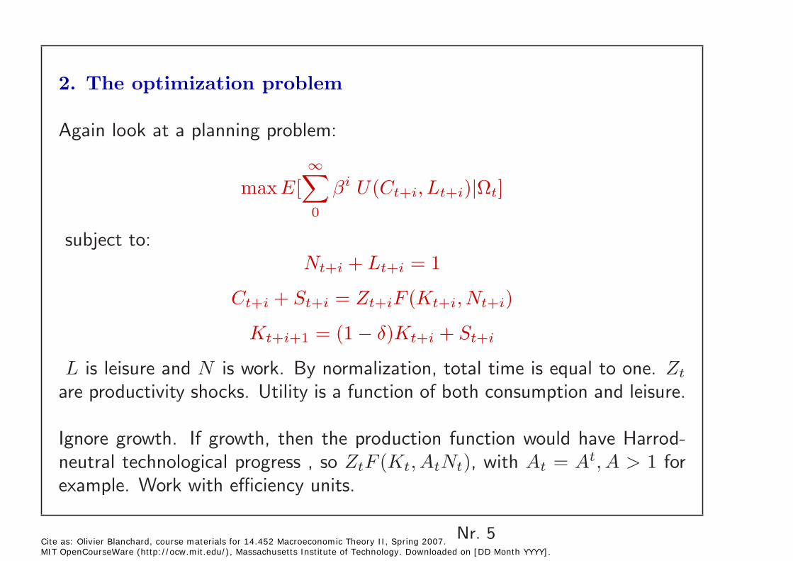
2. The optimization problem

Again look at a planning problem:

∞max E[

� βi U(Ct+i, Lt+i)|Ωt]

0

subject to: Nt+i + Lt+i = 1

Ct+i + St+i = Zt+iF (Kt+i, Nt+i)

Kt+i+1 = (1 − δ)Kt+i + St+i

L is leisure and N is work. By normalization, total time is equal to one. Zt

are productivity shocks. Utility is a function of both consumption and leisure.

Ignore growth. If growth, then the production function would have Harrodneutral technological progress , so ZtF (Kt, AtNt), with At = At, A > 1 for example. Work with efficiency units.


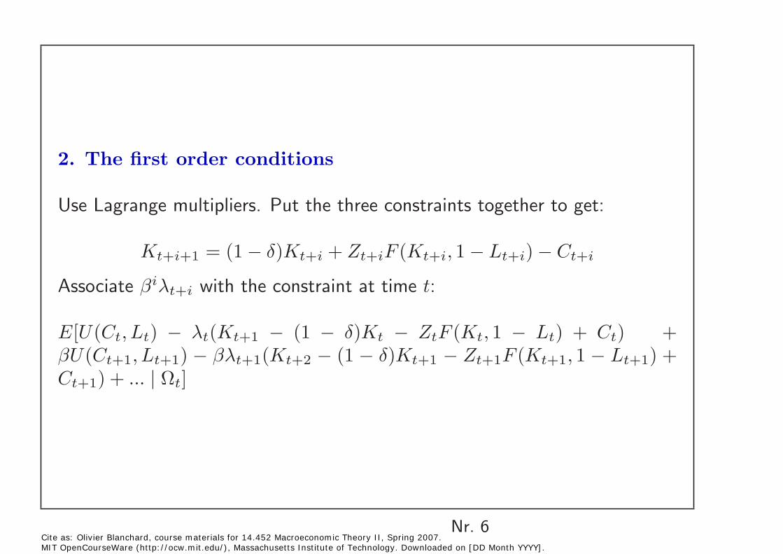
2. The first order conditions

Use Lagrange multipliers. Put the three constraints together to get:

Kt+i+1 = (1 − δ)Kt+i + Zt+iF (Kt+i, 1 − Lt+i) − Ct+i

Associate βiλt+i with the constraint at time t:

E[U(Ct, Lt) − λt(Kt+1 − (1 − δ)Kt − ZtF (Kt, 1 − Lt) + Ct) + βU(Ct+1, Lt+1) − βλt+1(Kt+2 − (1 − δ)Kt+1 − Zt+1F (Kt+1, 1 − Lt+1) + Ct+1) + ... | Ωt]


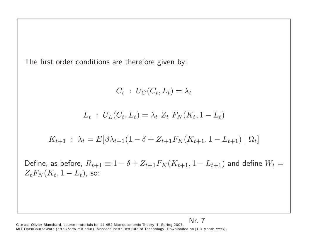
The first order conditions are therefore given by:

Ct : UC (Ct, Lt) = λt

Lt : UL(Ct, Lt) = λt Zt FN (Kt, 1 − Lt)

Kt+1 : λt = E[βλt+1(1 − δ + Zt+1FK (Kt+1, 1 − Lt+1) | Ωt]

Define, as before, Rt+1 ≡ 1 − δ + Zt+1FK (Kt+1, 1 − Lt+1) and define Wt =ZtFN (Kt, 1 − Lt), so:


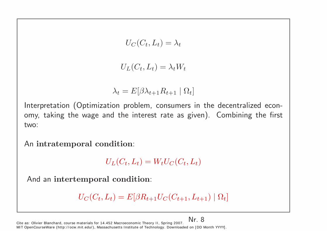
UC (Ct, Lt) = λt

UL(Ct, Lt) = λtWt

λt = E[βλt+1Rt+1 Ωt]| Interpretation (Optimization problem, consumers in the decentralized economy, taking the wage and the interest rate as given). Combining the first two:

An intratemporal condition:

UL(Ct, Lt) = WtUC (Ct, Lt)

And an intertemporal condition:

UC (Ct, Lt) = E[βRt+1UC (Ct+1, Lt+1) Ωt]|


Variational argument

UL(Ct, Lt) = WtUC (Ct, Lt)

Increase work by Δ, so decrease in utility of UL(Ct, Lt) Δ •

Increase consumption by WtΔ, so increase in utility of WtUC (Ct, Lt) Δ •

UC (Ct, Lt) = E[βRt+1UC (Ct+1, Lt+1) Ωt]|

Decrease consumption by Δ, so decrease in utility of UC (Ct, Lt)Δ•

• Save, and get Rt+1 next period, so an increase in expected utility of E[βUC (Ct+1, Lt+1) Rt+1 Ωt].|

Still: not easy to draw implications for general U(C, L).


62

3. Balanced growth path restrictions on utility?

Caveats. A clear trend in hours


Figure removed due to copyright restrictions.

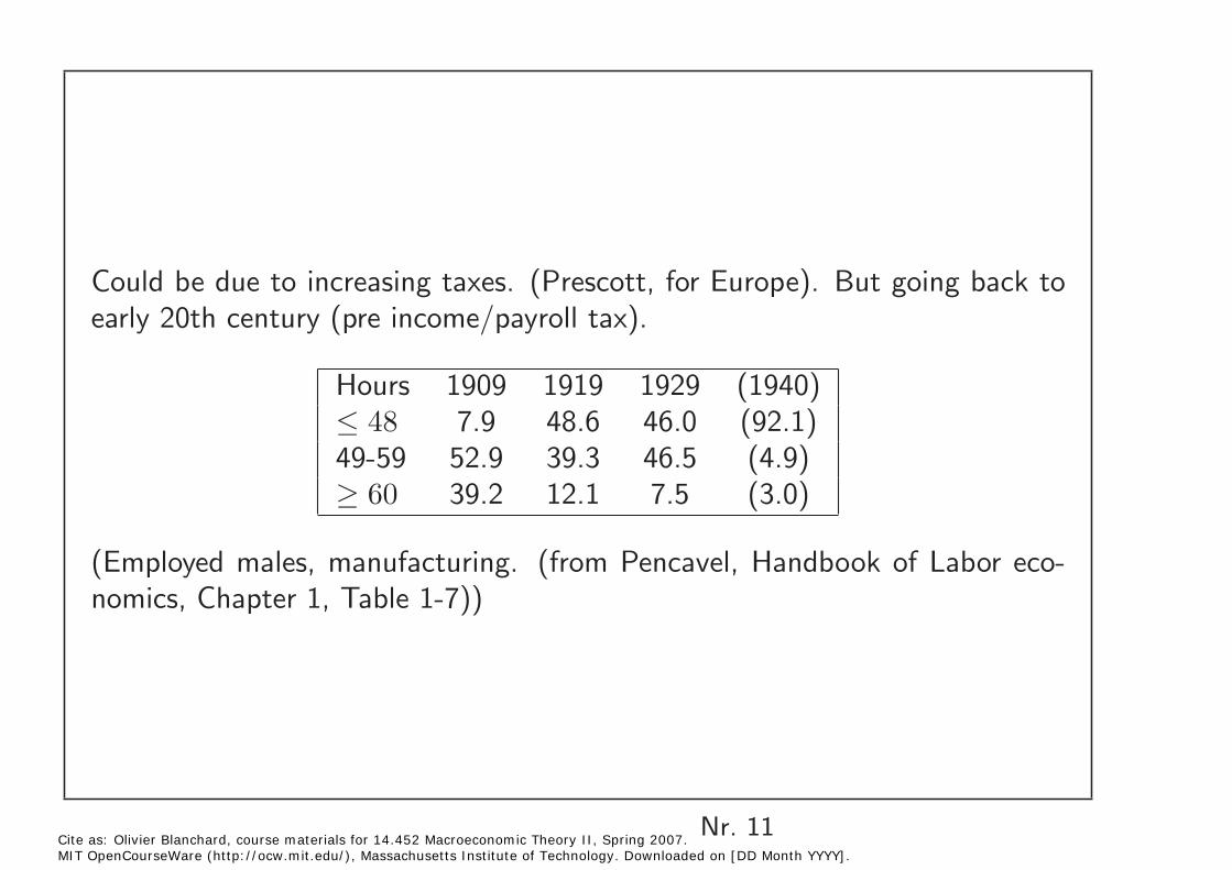
Could be due to increasing taxes. (Prescott, for Europe). But going back to early 20th century (pre income/payroll tax).

Hours 1909 1919 1929 (1940) ≤ 48 7.9 48.6 46.0 (92.1) 49-59 52.9 39.3 46.5 (4.9) ≥ 60 39.2 12.1 7.5 (3.0)

(Employed males, manufacturing. (from Pencavel, Handbook of Labor economics, Chapter 1, Table 1-7))


Is it reasonable to use balanced growth restrictions?

Additive separability in time implies strong short run implications. Will • be clear throughout course.

Put another way. Many specifications of preferences with same long run implications, different short run implications

U(C1 + C2, L1 + L2) + β2U(C3 + C4, L3 + L4) + ...

Home production versus leisure. •


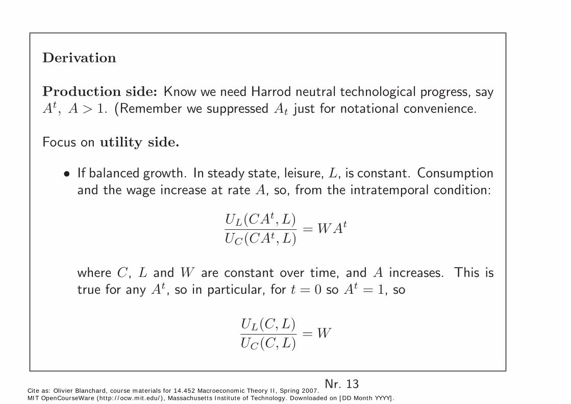
Derivation

Production side: Know we need Harrod neutral technological progress, say At, A > 1. (Remember we suppressed At just for notational convenience.

Focus on utility side.

If balanced growth. In steady state, leisure, L, is constant. Consumption • and the wage increase at rate A, so, from the intratemporal condition:

UL(CAt, L) = WAt

UC (CAt, L)

where C, L and W are constant over time, and A increases. This is true for any At, so in particular, for t = 0 so At = 1, so

UL(C, L) = W

UC (C, L)


Using the two relations to eliminate the wage, we can write:

UL(CAt, L) UL(C, L)= At

UC (CAt, L) UC (C, L)

The MRS between consumption and leisure must increase at rate A.

• This relation holds for any value of the term At So use for example At = 1/C:

UL(1, L)=

1 UL(C, L)UC (1, L) C UC (C, L)

Or, rearranging: UL(C, L) UL(1, L)

=C[ ]UC (C, L) UC (1, L)

The MRS must be equal to C times the term in brackets, which is a function only of L. For this to hold, the utility function must be of the form:

u(Cv(L))


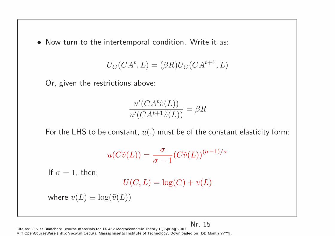
Now turn to the intertemporal condition. Write it as: •

UC (CAt, L) = (βR)UC (CAt+1, L)

Or, given the restrictions above:

u�(CAtv(L)) = βR

u�(CAt+1v(L))

For the LHS to be constant, u(.) must be of the constant elasticity form:

u(Cv(L)) = σ

(Cv(L))(σ−1)/σ

σ − 1

If σ = 1, then: U(C, L) = log(C) + v(L)

where v(L) ≡ log(v(L))


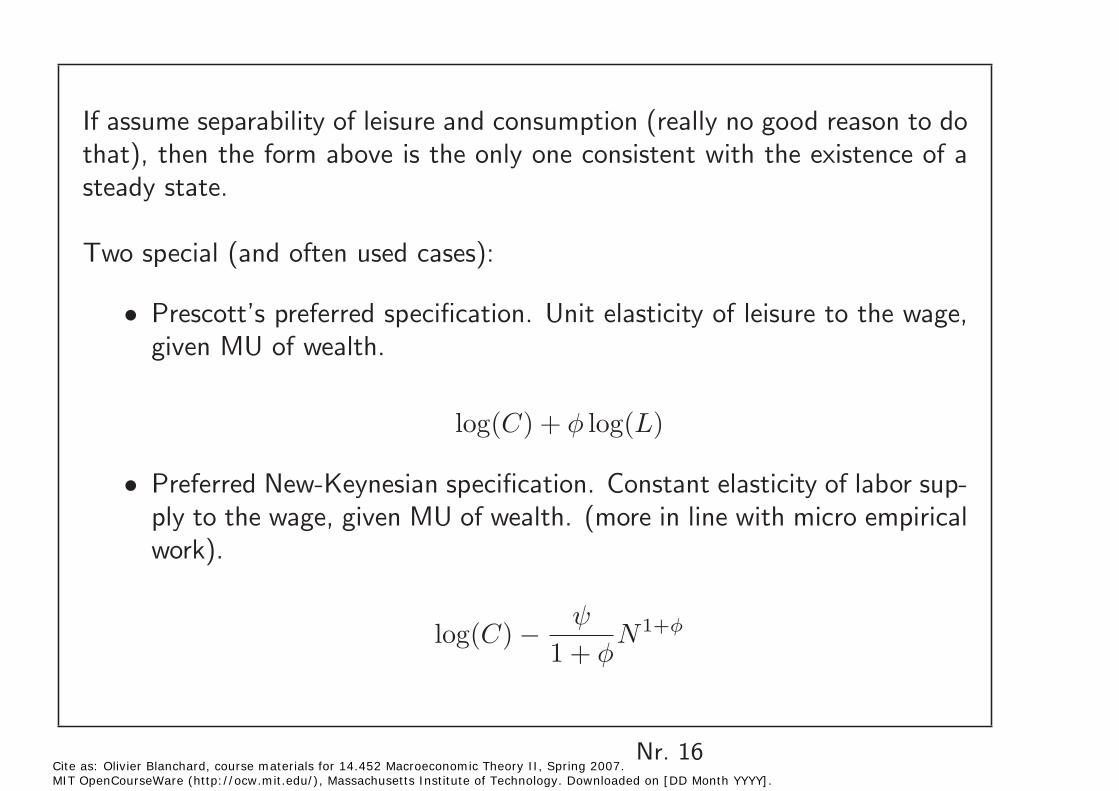
If assume separability of leisure and consumption (really no good reason to do that), then the form above is the only one consistent with the existence of a steady state.

Two special (and often used cases):

Prescott’s preferred specification. Unit elasticity of leisure to the wage, • given MU of wealth.

log(C) + φ log(L)

Preferred New-Keynesian specification. Constant elasticity of labor sup• ply to the wage, given MU of wealth. (more in line with micro empirical work).

ψlog(C) − N1+φ

1 + φ


4. Back to the FOCs

Use the specification U(C, L) = log(C) + v(L) and return to the first orderconditions:The intratemporal condition becomes:

v�(Lt) = Wt/Ct

The intertemporal condition becomes:

CtE[βRt+1 Ωt] = 1

Ct+1 |

Interpretation. (Note that UC = 1/C is the marginal value of wealth). So equalize marginal utility of leisure to the wage times the marginal value of wealth. And the Ramsey-Keynes condition for consumption.


Effects of a favorable technological shock? First pass. It increases W and R, both current and prospective.

Two effects on consumption. Smoothing (consumption up) and tilt• ing (consumption down). On net, plausibly up.

Turn to leisure/work. Two effects. •

A substitution effect: Higher Wt leads people to work harder.

An income/wealth effect. Higher Ct works the other way. As peoplefeel richer (1/C is the marginal value of wealth), they want to consumemore and enjoy more leisure.

Net effect depends on the strength of the two effects. Substitution(elasticity), and wealth (persistence).

In NK specification, using logs, n = (1/φ)(w − c).


The more transitory the shock, the smaller the increase in C, and so the • stronger the substitution effect.

If the shock is permanent, the stronger the wealth effect. Ct could• increase by more than Wt (but less than ZtF (Kt, Nt)). (Permanent shock to technology, plus capital accumulation). Employment could decrease.


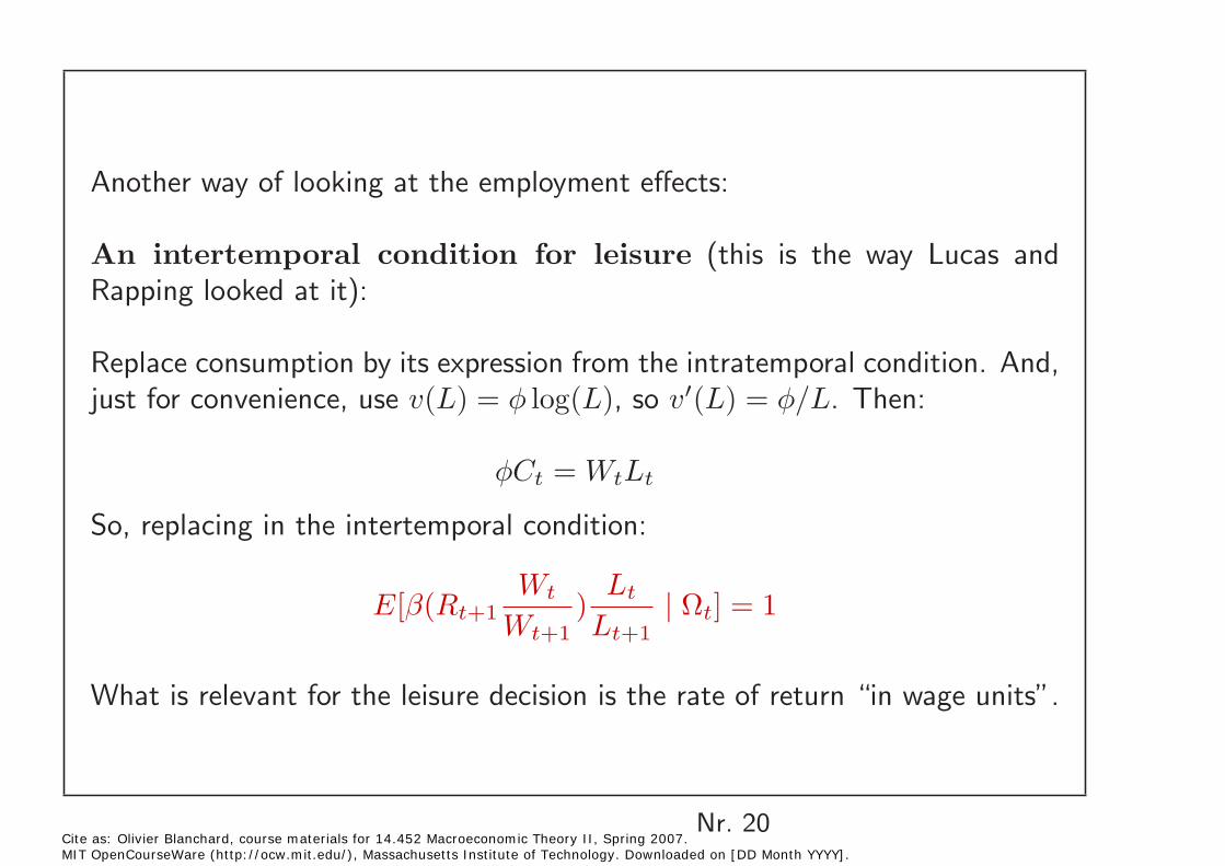
Another way of looking at the employment effects:

An intertemporal condition for leisure (this is the way Lucas and Rapping looked at it):

Replace consumption by its expression from the intratemporal condition. And, just for convenience, use v(L) = φ log(L), so v�(L) = φ/L. Then:

φCt = WtLt

So, replacing in the intertemporal condition:

E[β(Rt+1 Wt )

Lt Ωt] = 1Wt+1 Lt+1

|

What is relevant for the leisure decision is the rate of return “in wage units”.


• A transitory shock, so Wt increases but Wt+1 does not change much. Then Lt/Lt+1 will decrease sharply. Strong increase in employment.

• A permanent shock: Then Wt/Wt+1 is roughly constant, and so is Lt/Lt+1. (ignoring movements in R). No movement in employment.


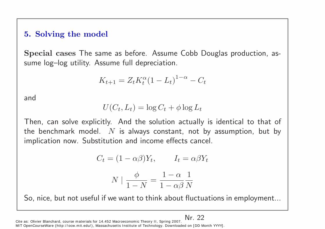
5. Solving the model

Special cases The same as before. Assume Cobb Douglas production, assume log–log utility. Assume full depreciation.

Kt+1 = ZtKtα(1 − Lt)

1−α − Ct

and U(Ct, Lt) = log Ct + φ log Lt

Then, can solve explicitly. And the solution actually is identical to that of the benchmark model. N is always constant, not by assumption, but by implication now. Substitution and income effects cancel.

Ct = (1 − αβ)Yt, It = αβYt

φ 1 − α 1 N =|

1 − N 1 − αβ N

So, nice, but not useful if we want to think about fluctuations in employment...


So need to go to numerical simulations. SDP, or log linearization. Campbell: Full analytical characterization for log linearized model; Otherwise, use explicit solution for log-linear system (use RBC.m, based on Uhlig, or use Dynare. )

The effects of different persistence parameters for the technological shocks. See figures from RBC.m for three values of ρ.

(Could do the same for different elasticities of labor supply, or different intertemporal elasticities. But in these two cases, you need to modify the matrices in RBC.m a bit. You may want to do it.)


Graph removed due to copyright restrictions.

Nr. 24Cite as: Olivier Blanchard, course materials for 14.452 Macroeconomic Theory II, Spring 2007. MIT OpenCourseWare (http://ocw.mit.edu/), Massachusetts Institute of Technology. Downloaded on [DD Month YYYY].

Table removed due to copyright restrictions.Table 1: Business Cycle Statistics for the U.S. Economy on page 938. King, R., and S. Rebelo. “Resuscitating Real Business Cycles.” Chapter 14 in Handbook of Macroeconomics. Vol. 1B. Edited by J. Taylor and M. Woodford. New York, NY: Elsevier, 1999. pp. 927-1007. ISBN: 9780444501578.


Table removed due to copyright restrictions. Table 3: Business Cycle Statistics for Basic RBC Model on page 957. King, R., and S. Rebelo. “Resuscitating Real Business Cycles.” Chapter 14 in Handbook of Macroeconomics. Vol. 1B. Edited by J. Taylor and M. Woodford. New York, NY: Elsevier, 1999. pp. 927-1007. ISBN: 9780444501578.


Figure removed due to copyright restrictions. Figure 7: Basic Model: Simulated Business Cycles on page 959. King, R., and S. Rebelo. “Resuscitating Real Business Cycles.” Chapter 14 in Handbook of Macroeconomics. Vol. 1B. Edited by J. Taylor and M. Woodford. New York, NY: Elsevier, 1999. pp. 927-1007. ISBN: 9780444501578.


Summary

Intertemporal and intratemporal conditions.•

Productivity shocks, consumption, and employment •

Too good to be true? •


olivier blanchard april 8, 2007 - mit opencourseware · 14.452. topic 3. rbcs olivier blanchard...

Documents