ON THE CLASSIFICATION STATISTIC OF l~TALD

by

Mohammad IqbalUniversity of North Carolina

This research was supported in part bythe Office of Naval Research under ContractNo. NR-042031 for research in probabilityand statistics at Chapel Hill. Reproductionfor any purpose of the United States Govern­ment is permitted.

Institute of StatisticsJvTimeograph Series No. 159November 1956

ERRATA SHEET

6(11)

141(6)

NotationiV(18)4(12)

13(2)

19(9)

21(5)

21( 6)

22(1)

92(3) will mean page 92, line 3 •Replace m = m3 by w = I m3 IReplace Z by z .

RePlace.//Nl+N2 byV NI N2

2 2Replace ~~ - m3 ~ 0 by ~m2 - m3 ~ 0

Re ad N( e ) as N •2 e

Replace (1- ~ by (1 _ ~)2 •n n

Replace 28 by a~

02gRead as , Q'

2 '0 all t'

23(1) From - ~n to the end of line 2, is to be enclosed in squareh brackets.

24(6) Put) after ~.n

27(!~) Put t"./ between II and III .

29(18) Replace f(x) by If(x) I and 0 :: c :: 00 by 0 ::: c < 00

48(7) Insert a multiplier ~ on the right.51(5) Replace 16 by 64 • (and this corresponds to p = 2.)62(9),113(7) Replace nm

3by Inm

3\

62(18), 92(3),115(7) Replace m3

by Im31 ~

69(1,5) Replace 1¢(t)-¢(t)1 by I¢(t) - ¢(t)l.

70(14), 88(16) Replace e- j bye-V•

81(9) Put dv: after Ie (v)m

85(7) Read 'yJ (v) = • 290(5) Replace ~ by ~ •103(5) Read l: as 1: •

T) n

119(15) Replace V > nm3 by IVI > Inm31 •_J.'X-2 -1 A.2

2 2135(11) Replace e by e139(18) Replace suffices by suffixes •140(6),(10) Replace r by y.

a ij ) 2a ijReplace -=r by

aij d atj

Read )(i as Jtl and 145(7) Read a;~ as aijz i •

•\

A C K N a ~ LED GEM E N T S

I wish to put on recqrd my deep sense of gratitude to

Professor Harold Hotelling for his inspiring guidance throughout

the preparation of this work. I feel myself greatly honored on

having had the privilege of working under his direction.

I am also greatly indebted to Professor R. C. nose for the

confidence derived through his encouragement at various stages.

My thanvs are also due to the Fulbright Foundation in Pa1(istan,

the Institute of International Education and the Office of Naval Re-

search for their financial assistance which made this study possible.

The help of Mrs. Kattsoff, Mrs. Spencer and Mrs. Kiley for the

careful typing of the manuscript is gratefully acknowledged.

Mohammad Iqbal

•

I®O scientific investigation can be final;it merely represents the most probableconclusions which can be drawn from thedata at the disposal of the writer. Awider range of facts or more refinedanalysis, experiment and observation willlead to new formulae and new theories.This is the essence of scientific progress.1!

Karl Pearson 1898

•

TABLE OF CONTENTS

CHAPTER

iii

PAGE

. . . . . . . . . . .

I.

ACKNOWLEDGEMENT

INTRODUCTION

A P~OBLEM OF CLASSIFICATION CONSIDERED BY WALD . . . .

ii

vii

1

1. Introduction. • . .. • .

2. Statement of the problem •.

3. An example of its importance

4. The statistic proposed by ir/ald

5. Further work on the problem

· .

. . . 1

3

5

5

9

II. ON AN ASYMPTOTIC EVA,LU~TI01\T OF /1 TRIPLE INTEGRAL.

1. Introduction

2. The integral and its domain

3. Order of the variables ml , m2 and mj

).+ • An important limit . · · ·5. A triple integral . · · .6. The integral over ~, an asymptotic approximation

7. An upper bound to error • · · · · ·8. The integral over D2 • ·9. An upper bound to the value of 12 • ·

10. Comparison of II and 12 . . · · . . .11. The integral over the domain D* • · . . . .12. Summary of Chapter II · · · .

12

12

12

14

18

25

29

34

43

48

51

53

5rr

CHAPTER

III. ON THE ASYMPTOTIC DISTRIBUTION OF T~ALDI S CL .'\SSIFIC:,-

iv

PAGE

TleN ST'TISTIC ••••

1. Introduction.

• • • • 0 oJ Q • 60

60

? lATald I s approximate classification st.9tistic andits moments • • • • • • • • • . 61

3. The asymptotic distribution of v for p = 2m

4. An integral equation due to Wilks

5. A note on Bessel functions

6. Distribution of v for odd values of p

66

75

76

79

7. The use of a differential equation in the evalua-tion of an integral • • •• ••••••.•••• 81

8. The asymptotic distribution of v for even andodd values of p ••••••• • • •• 82

9. Note on the construction of tables •. . ,. .. . . . . 88

10. Summary of Chapter III ••.••••• . . • . • 91

IV. AN~SYl'1PTOTIC SERIES EXP:\NSIOl\T FOR THE DISTRIBUTION OF

. . . .1. Introduction ••

2. An asymptotic series for the distribution

92

92

93

3. The constant of integration for the first approxi-mation • . • . • • • • 108

4. The tail are8S for the first approximation 110

5. Comparison with the results of Chapter III 113

6. Summary of Chapter IV 115

..

V. THE APPLIC'TI0N OF TCHEBYCHEFF-M,iRKOFF INE0UALITIES

v

6. Some results due to Tschebycheff and Narkoff

2. The integral over Dl

3. The integr al over D2 · . . · • ·4. The integral over D · . . . · · · .5. Moments of V • . . . . . . · · ·

TO A SPECT~L CASE • •

1. Introduction

. .

· .

116

116

lIS

117

119

119

120

7. tpplication of Tschebycheff-Markoff theorems tothis case . . . . . . . . . . .. 123

• • • • • • • • • • • • It • • • • •VI. NON-NULL C:\SE

1. Introduction • • • • i • • • • • · .128

128

2. The joint distribution '" • • ;, • • • • • •• 129

3. Note on confluent hyper geometric functions · · ·4. ~n asymptotic form of f(~, m2, m

3) . . .

5. Distribution of U for large n and p ::: 1, anindependent approach · . . · · · · · ·

6. The asymptotic mean and variance of the stC3tisticU . . . . . .. . . . . . · . . · · · · · ·

7. Correction term for the variance of the lineardiscriminant function · · . · · · ·

VII. SOME REL:ITED UNSOLVED PRORLE11S

130

132

133

137

145

148

1. On classification statistics of ~rTald and Anderson 148

2. The quadratic discriminators

Possibility of a differsnt approach · .148

150

CH'PT~

4. Efficiency. . . . • • •

5. The gre ater me"ln vector

BT~LI00R~PFY . . . . . . . . .

vi

P·:GE

150

151

152

..vii

INTRODUCTIONl

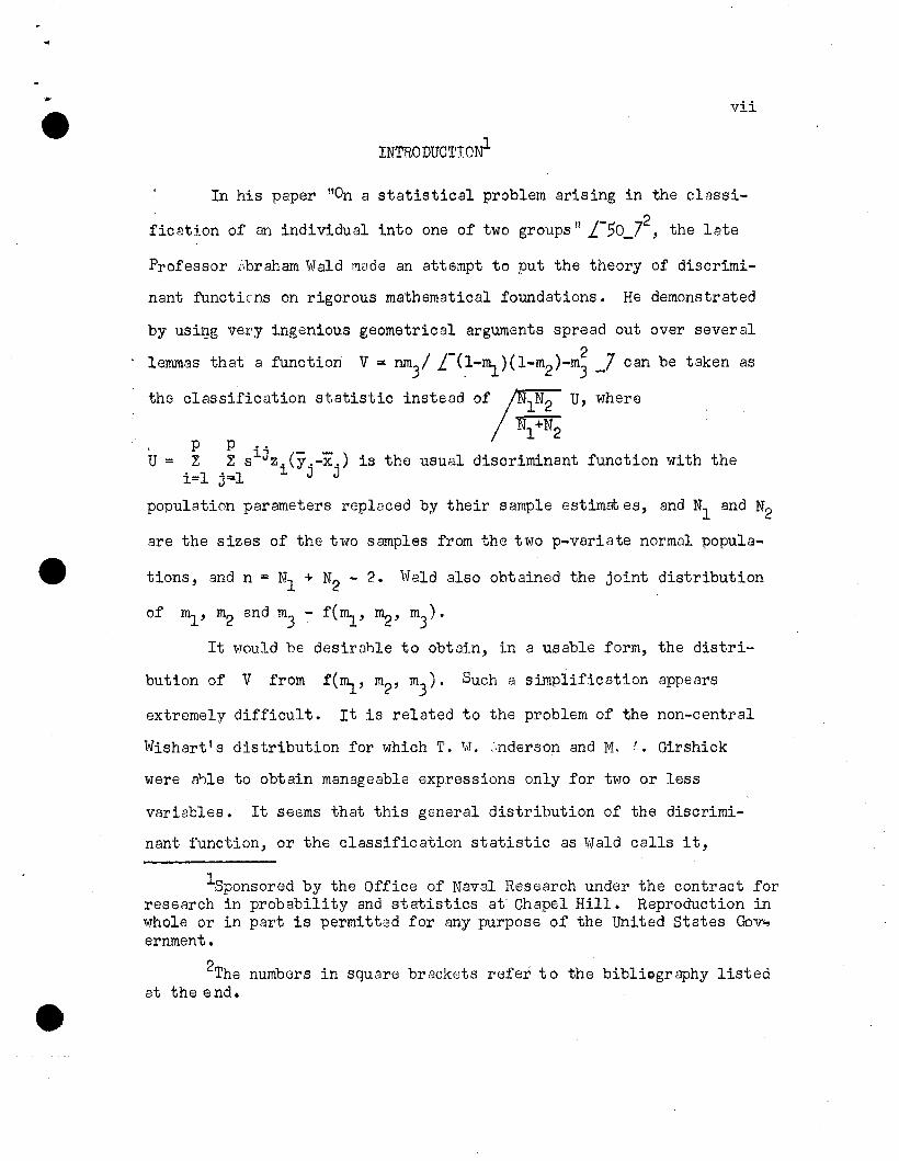
In his paper rtOn a statistical problem arising in the classi­

fication of an individual into one of two groups!! L-50_72, the late

Professor ~braham Wald Mude an attempt to put the theory of discrimi­

nant functicns on rigorous mathematical foundations. He demonstrated

p p ..lJ (- -)U = ~ Z s z. y,-x

jis the usual discriminant function with the

i=l j=l 1 J

by usi~g very ingenious geometrical arguments spread out over several

lemm,9s that a function V = nm3! L-(1-~)(l-m2)-m~ _7 can be taken as

the classification statistic instead of /NIN2 U, where!~~! Nl +N2

population parameters replaced by their sample estim~es, and Nl and N2

are the sizes of the two samples from the two p-variate normal popula-

tions, and n = Nl + N2 - 2. Weld also obtained the joint distribution

of ~,m2 and m3 - f(~, m2, m3).

It would be desirahle to obtain, in a usable form, the distri­

bution of V from f(~, m2, m3

). Such a simplification appears

extremely difficult. It is related to the problem of the non-central

lNishart I s distribution for which T. llJ. :,nderson and M. :'. Girshick

were a~le to obtain manageable expressions only for two or less

variables. It seems that this general distribution of the discrimi­

nant function, or the classification statistic as Wald calls it,

ISponsored by the Office of Naval Research under the contract forresearch in probability and statistics at" Chapel Hill. Reproduction inwhole or in part is permitted for any purpose of the United States Gov~

ernment.

2The numbers in square brackets refer to the bibliography listedat the end.

·e

viii

would involve the figurative distance, 6, between the centers of the

two populations. One approach to this highly involved distribution

would be to obtain a series of powers of 6 with each coefficient in-

volving nand p. The present work is chiefly concerned with the

examination of the first term of this series with special attention

to its value when n is large.

In the first chcp ter of the present work, a brief historical

introduction to the theory of discriminant functions is f~llowed by

a mathematical formulat ion of the problem following lrJald. The re-

sults obtained.by him and also by some subsequent workers on the orob-

lem are briefly described.

The next two chapters deal with the problem of findiDg the dis-

tribution of V in the null case, by supposing that n ~ Nl +N2 - 2

is a lar~e number. Explicitly this problem can be stated as follows:

p-3 n-p-l

Given f(ml,m2,m3)dmldm2d~= Canst. IlVl j2l1-1'11~ d~dm2d~

to find the distribution of V suitable

It will be noticed that the sample sizes, Nl and N2, do not

separately occur in the joint distribution and the assumption that n

is large, which is obviously milder than the assumption that Nl and

N2 are both large, introduces certain simplifications. One mmplifi-

cation that is obtained is that the statistic itself approximates

...

..

ix

because of the order in probability of the variables entering into the

distribution. The same ass~ption entails simplifications both in the

integrand and in the domain of integration.

In the second chapter, which can be regarded as dealing with

the mathematical aspects of the prcblem, methods have been developed

which will enable us to evalu ate triple integr als giving the moments

An upper bound to the error in using these simpli-

fications is also worked out which enables us to put reliance in the

aporoximations in suttable cases.

The third chapter deals TAith theaaymptotic distribution prob-

lem. 4fter £inding an expression for the kth moment of v, we obtain

the asymptotic distribution of v both for even and for odd values

of p. For even values of p, the uniqueness of the distribution, which

i~obtained by the help of its moment generating function, is also es-

tablished. For odd values of p, use had to be made of an integral

equation due to S. S. Wilks /-55 7; and, because of the fact that we- -are considering only the principal term in the kth moment.f v, the

uniqueness of the result cannot be guaranteed. This section is there-

fore presented on a heuristic basis and has to be left for further

discussion and rigorization.

In Chapter IV we have obtained an asymptotic series for the dis­

tribution of w = Im31 ,which is proportional to v. This is done

by observing that fora fixed w the range of integration for ~ and

m2 is a lenticular region enclosed by two hyperbolic arcs in the plane,

x

w c a constant. Integration is carried out over this region by using

suitable transformations, and the first three terms of the asymptotic

series are obtained. For the first approximation, we have also dis-

cussed the method of finding the tail areas.

Chapter V deals with the special case Nl + N2 = 20, P = 3•

. In this case, the first seven moments of V are found, and use is

made of the inequalities due to Tchebycheff and Markoff in setting up

bounds on probabilities of the type p(V ~ ~)~ These limits are rather

crude due to the fact that a small numher of moments is being used.

The example, however, illustrates ene way of proceeding to disc~ver

something about an unknown distribution when its first few moments are

known.

Chapter VI contains a few remarks on the non-~ull caso. It

starts with expressing the joint distribution of ml , m2 and m3

dis­

cussed by Sitgreaves /-45' 7 in another form suitable for large n.- -This chapter also contains a brief discussion of the asymptotic distri-

bution of U for p = 1. In the next section we exemplify the differ­

ential method by finding the mean and variance of U. The concluding

section of this chapter deals with finding the variance of the linear

discriminant function when the sampling fluctuations of the means are

tck en into account. In the last chapter are listed a few unsolved prob-

lems related to the problem of classification.

CHAPTER I

A PROBLEM OF CLASSIFICATION CONSIDERED BY WALD

1. Introduction.

The problem of classification ie the problem of assigning an

individual (or an element), on which a set of measurements is avail-

able, to one of several groups or populations. The problem admits

a simple solution when the distributions of measurements in the al-

ternative populations are completely kncwn or what is the same thing

as saying that the sizes of the samples available from the various

populations, on the basis of which we have to make a decision, tend

to infinity, so that the sample estimates of the parameters tend

stochastically to their population values. If, however, the samples

are not +arge, the problem becomes rather complicated~

Research in this area of Multivariate Analysis was started wi. th

his introduction of the linear discriminant function by Sir Ronald A.

Fisher L-IO_7 in 1936. The linear discriminant function is

PD = Z f.zi, in which z = (zl ••• zp) is the new observation, and

i=l ~

the coefficients Ii' following Fisher, can be obtained by maximizing

the square of the difference of the expectations of D in the two

populations divided by the standard deviation of D. The linear dis-

criminant function provides the best solution of the problem of classi-

fication provided that,

(1) The number of alternative populations is two,

(2) The form of the distributions in both populations is

2

multivariate normal,

(3) The parameters are all known,

(4) The covariance matrj.ces of the two populations are equal.

It may be remarked that Welch L-53_7 observed that even

without making any assumptions of normality or equality of covar-

iance matrices, the problem of obtaining the best function to dis-

crim:i.nate between t1>10 completely specified populations may be

solved. He demonstrated that the desired function is simply the

ratio of the two probability distributions, and the criterian level

to which this function is referred is deducible either from Bayes l

Theorem with given a priori probabilities or by the use of a lemma

by Neyman and Fe arson L-)2 7 when the errors for the two hypotheses

are minimized in any given ratio. He proved that under the four

assumptions stated nbove the function obtained in this manner is

identical with the linear discriminant function,

Von Mises ~3l_7 considered the problem of classification

when the number of populations is m, and showed how to subdivide the

s3mple space into m parts so as to minimize the maximum error of

misclassification.

Rao /-39 7 gave explicit Bayes solutions with given a priori- -probabilities or ratios of errors for the alternative populations,

and discussed the construction and use of doubtful regions and re-

lated problems.

3

In all these cases it is assumed that the distributions are

completoly specified. If, however, as will frequently be the case,

one cannot justify the supposition that the distributions are com-

pletoly known, and the only information at hand is what is contain-

ed in the samples available from various populations, we run into

rather complicated distribution problems.

W':lld L"1;o _7 in 1944 set out to solVG the problem of classi-

fication for the case of two altern[ffiivG populations. Instead of

using a distri.bution-free approach he si.mplified it further by in-

troducing the following two restrictionsl

(1) The form of the distributions is multivariate normal.

(2) The two populations have the same covariance matrix.

Though it would be desirable to solve the problem without.

making either of these assumptions, still one can argue that in

many practical problems arising in numerous fj.elds of scientific

inquiry it is not unreasonable to make the two assumptions stated

above.

In this chapter we propose to give a mathematical formula-

tion of the problem, and to state the conclusions of Wald, and of

subsequent workers on the problem.

2. Statement of the problem.

/#

xll x12 . · • xlp

(2.1) Let Xx2l x2p

=

. • . . • ·xN 1 · • x

1 NIP/"

4

,./

Yll Y12 · • · YIp

Y2l · • · Y2p(2.2) and y=

· · •

YN 1 · · · YN P2 2·

be two random samples from two variate normal populations )(x

and jf both having the same, though unknown, covariance matrixY

E, and different Unknown mean vectors

Let

and

respectively.

be an observation on a new individual which is known to have come

either from lTx or from Jry' but is distributed independently

of both x = (xl'" xp) and Y = (YI ... yp)' the two sets of

variates corresponding to 1T and 1T respectively.x . Y

On the basis of the information supplied by X, Y and Z the

such that if the probability of one type of misclassification is

held fixed, the chnnce of second typo of misclassification is min-

imum.

3. As an example of the importance of this problem we can con-

sider a candidate applying for admission to an institution with

certain test scores. He may have t~ be accepted or rejected de-

pending on his chances of success or otherwise on the basis of the

scores of candidates admitted in previous years.

4. the statistic proposed by 1liald.

(4.~ Wald considered as classification statistic

p P i'J (- -)U = Z Z s z. y. - x ji=l j=l ~ Jobtained by considering this problem

as one in testing the hypothesis

tive that

H: Z&}Tx "x against the alterna~

and by replacing the population values of the parameters by their

optirnum estimates obtained from the samples in the statistic ob-

tained by using the fUl)damental lemma of Neyman and Pearson. Thus

'where

(4.2)

and

e.

-x. =~

Nl 'I"~Ex N

a=l iat 1

The statistic U can be rewritten as

6

where

(4.5)

and where

and

are distributed independently of each other according to p-variate

normal distributions with

E (z) =

and

{: if z e Jtxif z e rry

,

and with the same covarinnce matrix /-a.. 7.- l.J-

Since the Sij are distributed independently of the set

( ~~

zl •.• zp' zl

if we define

•••~}

z ), the distribution ofp

n 2 /s .. = Z t

i/ n ,

l.J 0;..1 aI

U remains unchanged

where

and writing

bution of U

n => Nl + N2 - 2

i' 1(s J) for (s, ,)- , W31d observed that the distri­~J

is the same as that of

7

(4.7)p

V == Ei=l

P 'jZ s~ t t. 2

, 1 i,n+l J ,n+J"'"

whore the probability element of t ia is given by

1/- p n

t:(4.8)(2n)P(2+2)

exp /-~ Z E +

L i=l a=l ~a

7 p n+2p

)2+P

i)2Z (t - Z (t - / IT "IT dtiai=l i,n+1 i i=l i,n+2 _/ i=l a=l

whcO're

(4.9) p= Cf'1 p 2 . . . p )p

~ = (t. t tp)- 1'''' 2 . . .

are certain functions of ~i' vi and Gij , 1, j ~ 1, 2 •.• p.

Here Wald introduced two sets of numbers (ul ••• un+2) and

••• ' v 2)n+ satisfying the relations

(J.J. .10)n+2 2 n+2 2Zu=Zv=l

a=l a, a=l aand

n+2Z u v = 0

a,=1 a a

~nd using a very ingenious geometrica~ argument, concluded that the

distribution of V

(4,11)

where

(4.12)

is the same as that of

eu2m == ~

10:=1 a:

and the joint pl'obabi..1ity distd.bution of ~,m2 and ID3

is given by

,/ r ~ n+?-lJ.r11

, , , \ --.,.-Ip ).E

, . .dm1om?dm

3•

r p1 r. . • . pp

"'~ /

t'lhere r ijp

= Z t. t ja=1 ~a aand g is the constant of integration, in

9

tho domain 0 ~ ~ ~ 1, 0 .: m:, :: 1, - v'~m? ~ m3 :: v'~~ , and

zero othEJrwise;

where

and

F (t) ~.k

1 ,

5. ~rther ·W~rk on the problem.

Anderson [' 1;..7 considered the statistic

(5.1) ij (- -) 1 ij (- - )(- - )W=~ Z s zi Yj-XJ, - ~ Z ~ S Yj+X. Yj-x.

i j ~ i j J- J

which is much like U, since it differs from U by terms independent

of Z =(Zl ••• zp)' the measurements observed on the new in­

dividual. He c;valuated the expected value of the matrix of non-

central Wishart variates occuring in the joint distribution of ml

,

m? and m3

in the special case when

(5.2)

Sitgreaves L-45 _7 gave an analytio derivation of the dis~

tribution of W in the case considered by Anderson ond also obtain-

ed exactlythe constant of integration in the joint distribution

10

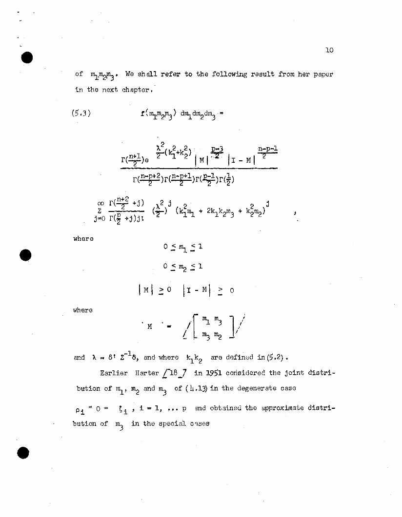
of ~m2(l13. We shall refer to the following result from her paper

in the next chapter.

where

,

where

> 0- !I-MI> 0

and ~ = 6' Z-15, and where k1k2 are defined in (5.2) •

Earlier Harter L-18_7 in 1951 corisidared the joint distri­

bution of ~, m2 and m3

of (4.13) in the degem~rate case

Pi = 0 == ~ i ' i == 1, ,.. p and obt ained the approximate distri-

bution of m3

in the special cases

11

(I-a) n even, p odd

(I-b) n even, p even.

The technique he used in deriving this distribution was

ossontially exp,~ding the two binomials constituting the integrand

in the joint distribution of ~, m2 and m3 of (4.13)in tile degen­

erate case, and integrating with respect to ml and then with re­

spect to m2 , The number of terms in the distribution of m3

thus

obtained deponds on n, which is not a small number in any practical

situ3tion. Moreover the solution thus obtained is not an asymptotic

series in which the leading terms could be considered as approxi-

mating the true distribution for large n.

The latest paper in historical order of development of the

theory of discrimination is that of Rao /-40 7, in which he devel-- -oped some general methods by using the ic1e.as of sufficient statis­

tics and fiducial probability distributions, by using Which, the

discrimination problem can be solved utilizing only the sample in­

formation. 'The distribution problems connected with the test

criteria suggested in the p3per have, however, yet to be tackled,

CHAPrER II

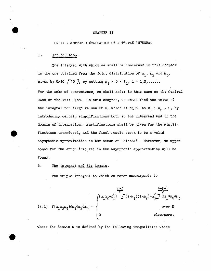
ON p~ ASYMPTOTIC EVALUATION OF A TRIPLE INTEGRAL

1. Introduction.

The integral with which we shall be concerned in this chapter

is the one obtained from the joint distribution of ml , m2 and m3

,

given by Wald ~50_7, by putting Pi = 0 = ~i' 1 ~ l,2, ••• ,p.

For the sake of convenience, we shall refer to this case as the Central

Case or the Null Case. In this chapter, we shall find the value of

the integral for large values of n, which is equal to Nl + N2 - 2, by

introducing certain simplifications both in the integ~and and in the

domain of integration. Justifications shall be given for the simpli-

fications introduced, and the final result shown to be a valid

asymptotic apnroximation in the sense of Poincare. Moreover, an upper

bound for the error involved in the asymptotic approximation will be

found.

2 • ~ integral and ~ domain.

The triple integral to which we refer corresponds to

o

over D

elsewhere.

where the domain D is defined by the following inequalities which

insure a real, positive integrand in its interior.

13

(2.2) D:

The ine~ualities in (2.2) show that the domain is bounded

by two right elliptical cones in three-dimensional space having

vertices at (0,0,0) and (1,1,0) respectively and having a common

base in the plane ml + m2 = 1.

We def~ne two other domains Dl and D2 as follows:

(2.3)

O~ml~l

°~ ~ ~21mlm2 - m3 ?:: °m1 + m2 ~ 1

°:s ml ::; 1

0~m2=S1

(1-ml )(1-m2)2

- m > °3-

(2.4) Then it is easy to see that D =Dl + D2, except for the set

of points lying on the plane ml + m2 = 1, which are counted twice.

The truth of this statement can be seen easily by noticing

that the regions defined by the two domains are the interiors of

two cones, one obtainable from the other by a simple transformation

14

and lying on oppos i te 6 ides of the plane ml + m2 = 1 in the space

of three dimensions. Moreover, except for the points lying on the

plane ml + m2 = 1, the two regions are mutually exclusive because

the point set corresponding to Dl

lies on the origin side, whereas

the other corresponding to D2 lies on the non-origin side. The fact

that Dl and D2 between themselves include all the points of D can be

seen by observing that

2m~mr, - m3 2: 0,

.L c: 2(2.5) > (1-ml )(1-m2 ) - m3 2: OJml + m2 ~ 1

(1:'m1)( I-m2) 2and - m3 2: 0,

":> m1m2_ mC: > 0(2.6) ml + m2 2: 1 3- ,

~lhere ====~> is read as "imply".

As a consequence of this result, we can find the value of an

integral over D by adding up its values over the two domains Dl

and

D2 • The fact that points lying on the plane ml + m2 = 1 have been

taken twice would not make any difference because they form a set

of Lebsegue measure zero.

3. Order ~ the variables ml ,m2 and m3

,

To examine the order of the variables mI' m2 and my we have

15

first to define them following the original paper of Wald L-50_7.For the sake of clarity, therefore, we add the following paragraph.

Denote by S the 2n + 1 dimensional surface in the 2n + 4

dimensional space of the variables ul , •••un+2, vl , ••• vn+2 defined

by the following equations:

~2 n+2 22Zu =L v = 1~=l ~ ~=l ~

(3.1) n+2~ u~v~ = 0.

~=l

Let u1 .•.un+2, vl .••vn+2 be random variables whose joint

probability distribution function is defined as follows: the point

density function is defined by

dSps·s

Then for any subset A of S, the probability of A is equal to

the 2n + 1 dimensional value of A divided by JdS. It should be

noted that the probability density function (3.2) is identical with

the probability density function we would obtain if we were to assume

16

that ul , ••• ,un+2, vl , ••• ,vn+2 are independently, normally distributed

with zero means and unit variances and calculate the conditional den-

sity function under the restriction that the point (u1, ••• ,un+2,

v l ' ... ,vn+2 belongs to S.

Variables ml , m2 and m) which are equal respectively to

P 2i: ut3 '

(3=1

r 2L; v(3

13=1

can be redefined by using (2.1) as follows:

P 2 n+22ml = r u / L uf3

13=1 13 f3= 1

P 2n+2 2(3.3) m2 = L vf3 / I:. v

13=1 13=1 13

p / (n+2 ·2 n+22

m3

= r u v / L u13

l. vf3 ,(3=1 13 13/ V 13=1 f3=1

where p is the number of variables and n =

of degrees of freedom.

N + lIt - 2 is the numberr.::

With this explanation about the variables entering into the

discussion we shall prove the following theorem:

Theorem (1). The variables ml , m2 and mj

defined in (3.3) in

terms of u. and v., i=1,2, ••• ,n+2, which are N(O,l), variates; are of1 1

order n-l in the probability sense.

17

Definition. We write XN = 0 L:f(N} 7, and say that ~. is ofP I - IIJ,

probability order 0 L:f(N)_7 if for each € > 0 there exists an

A€ > 0 such that L:P I xN I ~ Ae f(N)_7 ~ l-e for all values of

N > NO(e),

Proof of the theorem:

Since u. and v., i=l, ••• ,n+2, are all independently, normally~ 1

distributed with zero means and unit variance,

(3.4) p-l )n-p+1mi

(I-m. dm., 1=1,21 1

since each of m1

and m2

is of the form

Thus

E(mi ) = -R- andn+2

p(n-p+2 )

(n+2}2(n+3)= o (12)

n

and by Tchebycheff's inequality, namely

(3.6) P

it is immediately seen that for given € there exist k l and k2

such

that

18

Hence ml and m2 are of order ~ in probability.

To see that m3

is also of order ~ in the probability sense,

we note that

n+2 2 n+2 2L:: u' L v·

13=1 (3 13=1 13

But

(3.10) therefore

P 2Y: u

1313=1n+2-­

2L u

13=1 (3

P 2L v

,8=1 13n+2 2

E v13=1 13

(3.11)

From this, by noting that ml = 0 (!) and m = 0 (l), we concludep n 2 p n

that1m

3= 0 (-) •p n

4. An important limit.

In this section we shall prove a result which will be he1p-

ful in finding asymptotic values of triple integrals of the type

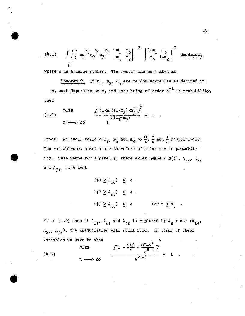
19

iff m VIm V2m v3 Iml m31 a Il-ml m3 Ib. 1 2, m, m2 m, I-m2

D

where b is a large number. The result can be stated as

Theorem 2. If ml , m2, m, are random variables as defined in

-1" each depending on n, and each being of order n in probability,

then

(4.2)pUm

n -> 00

1

Proof: We shall replace ml , m2 and m, by ~, ~ and *respectively.

The variables 0, ~ and r are therefore of order one in probab11-

ity. This means for a given €; there exist numbers N(e), Ale' A2€

and A3e

, such that

for n > N- e

If in (4.3) each of Ale' A2 € and A3€ is replaced by Ae = max (Ale'

A2e, A,e)' the inequalities will still hold. In terms of these

variables we have to show

plim

(4.4)n --i> 00

2 n_ ~+13 + OB-r 7

n 2-n

e -a-f3 = 1

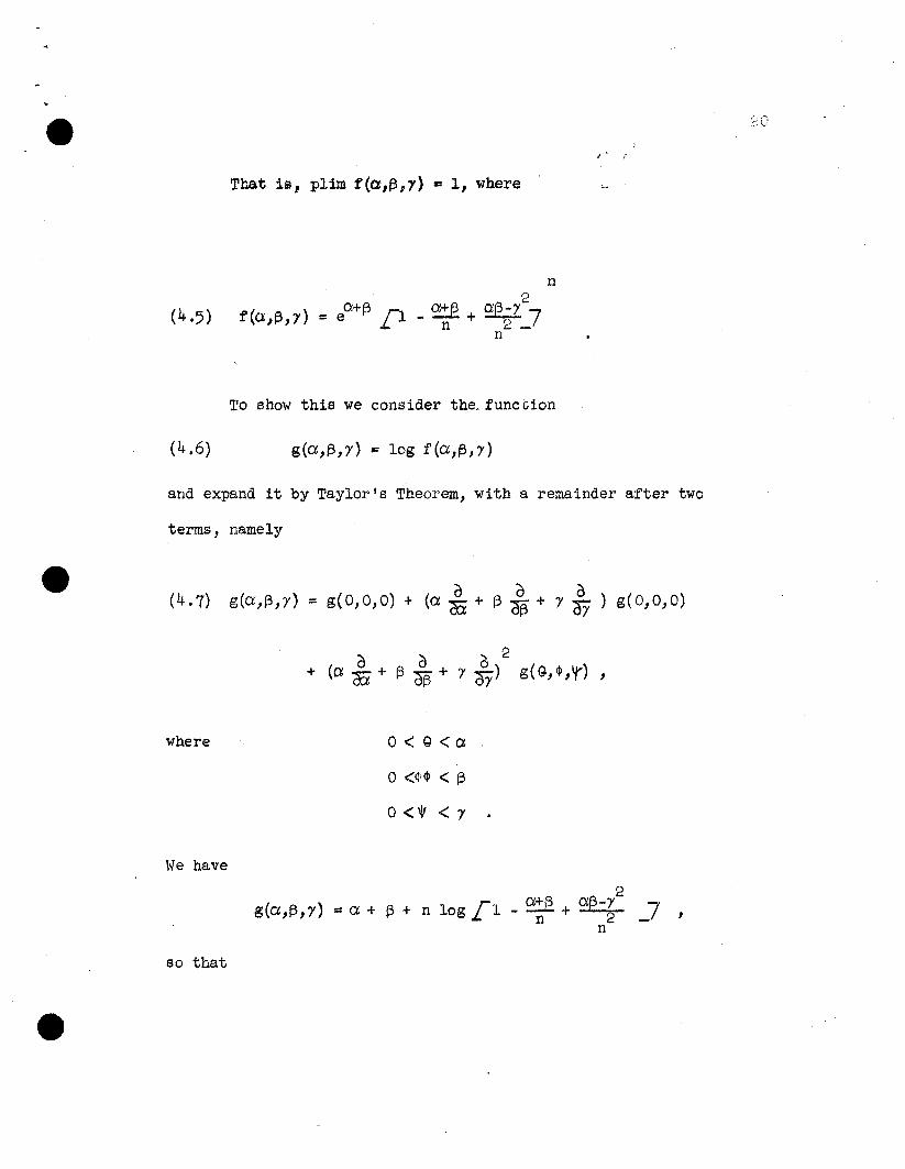
(4.6)

". ./

To show this we consider the;funccion

g(a,~,y) = log f(a,~,y)

20

and expand it by Taylor's Theorem, with a remainder after two

terms, namely

(4.7) g(o:,t3,y) = g(O,O,O) + (a.~ + f3'£- + y ~ )g(o,O,O)

o 0 ... 2+ (ex cti + f3 ~ + 1;Y) g(G,4>,r),

where

°<4;4> < f3

O<W <y

We have

2g(a,~,'Y) = a + ~ + n log £1 _ a~t3 + a~-~ _7 ,

n

so that

o 1.I3/n~=l- ... . 2

(1 - ~) (1 - ~) - r2n

a:og 1 ndi3 = 1 - ------~2

(1 _ ~)(l _~) 7n n --2

n

,

21

Also

2- 1:.(1 - ~)n n

,

2~2 - l (1 - ~o g n n ,dt)2 = 2 2

Ii(l - £) (1 - f?) - l.r; 7n n <::-n

2g If _ £ _ ~ + 213+ 7 7

2 n k~ n n 2-d g ndr2 =--------2--

2

I( 1 - ~) (1 - ~) - 12_7n

,

22

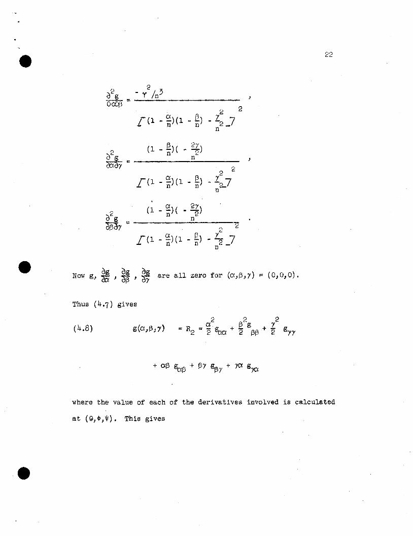
rl 2 :t.de; - Y /n-'-~ = ------------OCOfJ

(1 _~)( _ 2~)2 n cd g _ ....;... ~n~ _~-

.(1 _ £)( _ _21')

d2 n 2g ....;;;n;.....- "1>

~7 - 2 2ex f3 "I£(1 - -)(1 - ~) - {? 7n n n·-

,

dg dg dgNow g, di ' diB ' or are all zero for (a,f3,I') = (0,0,0).

Thus (4.7 ) gives

(4.8)

where the value of each of the derivatives involved is calculated

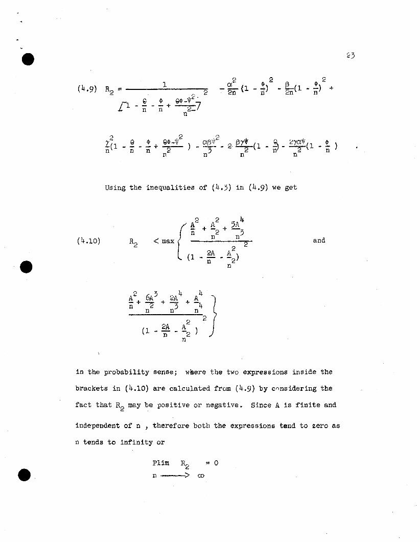
(4.9) 1 ci $2- ~{l

41 2R2 = --(l - ....) - -) +

r' 2 . 2n n 2n ng 41 '!rt::-

Ll - - - - + Q<I>- 7n n 2_

n

23

21(1n

_ t )n

(4.10)

Using the inellualities of (4.3) in (4.9) we get

2 22A A

(1 - Ii" - -2 )n

and

in the probability sense; where the two expressions inside the

brackets in (4.10) are calculated from (4.9) by c~nsidering the

fact that R2 may be positive or negative. Since A is finite and

independent of n , therefore both the expressions tend to zero as

n tends to infinity or

PUm R2 = 0

n > 00

24

Hence

2 n R2PUm eo.:+t.3 Tl _ a+f3 + et(3-1 7 = Plim e = 1L n 2-

n

That is, _ Ci+f3 + Cf,f3-y21 nn 2

nis asymptotically equivalent to

e ~-f3 ~n the b bOlot~ pro a 1 ~ Y sense. Note: An alternative proof of the

statement (4.2) shall be provided if we are able to prove that

(4.12) plim fn log (1

n:->co

c h- - + - +n 2

n

2where c stands for Cf, + (3 J and h = Cf,f3 - y and Ct,(3 and yare res-

tricted by the conditions (4.3).

It is easy to verify that

(4.13) -x xn:x ~ log (1- ii) $xn

x 3- -2

2n

in which the lower bound is written by observing that

2 3 2 3x x x x x x x- log(1 - Ii') :; n+ ~ + ~ + ••• ~ n + (n) + (n) + ••• ,

2n 3n;)

~'5

and both the -limits coverge to zero because of the restrictions

(4.3). This proves the statement (4.12) and hence the Theorem.

5 . ~ triple integral.

In this and the remaining sections of this chapter, we shall

confine ourselves to the study of the integral

(5.1) I = ffJD

where D is defined in (2.2) • To find an asymptotic approximation

to the value of I we first write

I = 11 + 12 '

26

where 11 and 12 denote the values of the integral over Dl and D2 -

To find 11

, we shall first evaluate the integral

IfJ

and then find an upper bound to

that is, an upper bound for the error committed in replacing the

n-p-l2 2

the factor ~(l-ml)(l-m) - m3 _7 in the integrand by

n- -(m + m2 )

e 2 1 Using (5.3) and (5_4), we can state that

It will then be demonstrated that both the error committed in

approximating 11 by III and the value of 12 are negligible as com-

pared to the least possible to value of I1

- Mathematically

Elim I ._ E = 0

11n->oo

27

and

lim

n -~ coI - E11

= 0 •

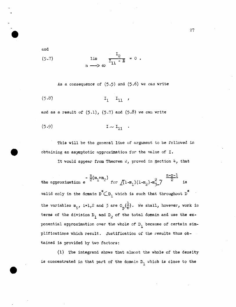
(5.8)

As a consequence of (5.5) and (5.6) we can write

and as a result of (5.1), (5.7) and (5.8) we can write

(5.9)

This will be the general line of argument to be followed in

obtaining an asymptotic approximation for the value of I.

It would appear from Theorem 2, proved in section 4, that

n n-p-l- 2'(ml +m2 ) 2 2

the approximation e for Ltl-ml )(1-m2)-m}-7 is

valid only in the domain D*C:Dl which is such that throughout D*

the variables m., 1=1,2 and 3 are 0 (!). We shall, however, work in~ p n

terms of the division Dl and D2 of the total domain and use the ex-

ponential approximation over the whole of Dl because of certain sim­

plifications which result. Justification of the results thus ob-

tained is prOVided by two factors:

(1) The integrand shows that almost the whole of the density

is concentrated in that part of the domain Dl which is close to the

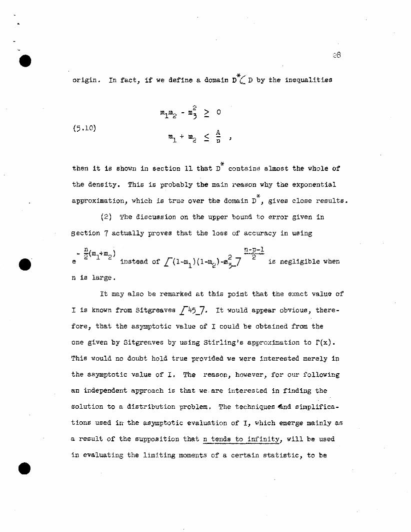
origin. */In fact, if we define a domain D LD by the inequalities

2 > 0ml m2 - m,

(5.10)Aml + m2 < - ,n

*then it 1s shown in section 11 that D contains almost the whole of

the density. This is probably the main reason why the exponential.x-

approximation, which is true over the domain D , gives close results.

(2) The discussion on the upper bound to error given in

section 7 actually proves that the loss of accuracy in using

n n-p-l- '2(ml+m2 ) 2 -2-

e instead of ~(1-ml)(1-m2)-m)-7 is negligible when

n is large.

It may also be remarked at this point that the exact value of

I 1s known from Sitgreaves ~45_7. It would appear obvious, there-

fore, that the as~~ptotic value of I could be obtained from the

one given by Sitgreaves by using Stirling's approximation to r(x).

This would no doubt hold true provided we were interested merely in

the asymptotic value of I. The reason, however, for our following

an independent approach is that we are interested in finding the

solution to a distribution problem. 'l'he techniques ~nd simplifica-

tions used in' the asymptotic evaluation of I, which emerge mainly as

a result of the supposition that n tends to infinity, will be used

in evaluating the limiting moments of a certain statistic, to be

called Wald's approximate classification statistic. This distribu-

tion problem will be our subject of discussion 1n chapter III.

6. The integral over Dl1 an asymptotic approximation.

ffp-3· E.:f!

(6 .1) Let Ii • I ("'1m2-m~) 2 lfl-"'J.)(1-m,J -m;"7 d"'J.dm2dm3,

Dl

where Dl is defined by the following inequalities:

2 > 0m1m2 - m3m1 + m2 < 1

(6.2)0 ~ m1 .< 1

0 ~ m2 < 1 j

and where m1

= 0 (1:.) for 1=1,2, and 3. We shall replace the secondp n

n- 2(ml+m2 )

factor in (6.1) bye, but the operation of integration

after this replacement needs some justification. There is no loss

of generality if we consider a similar univariate case and prove

that it is possible to replace a binomial raised to a large power by

an exponential factor to which it increases. We shall state this

result formally as

Lemma. Let rex) be a function of the real variable x, such that

Then

rex) < A if 0 =:; x ~ c, where 0 < c < 00.

30

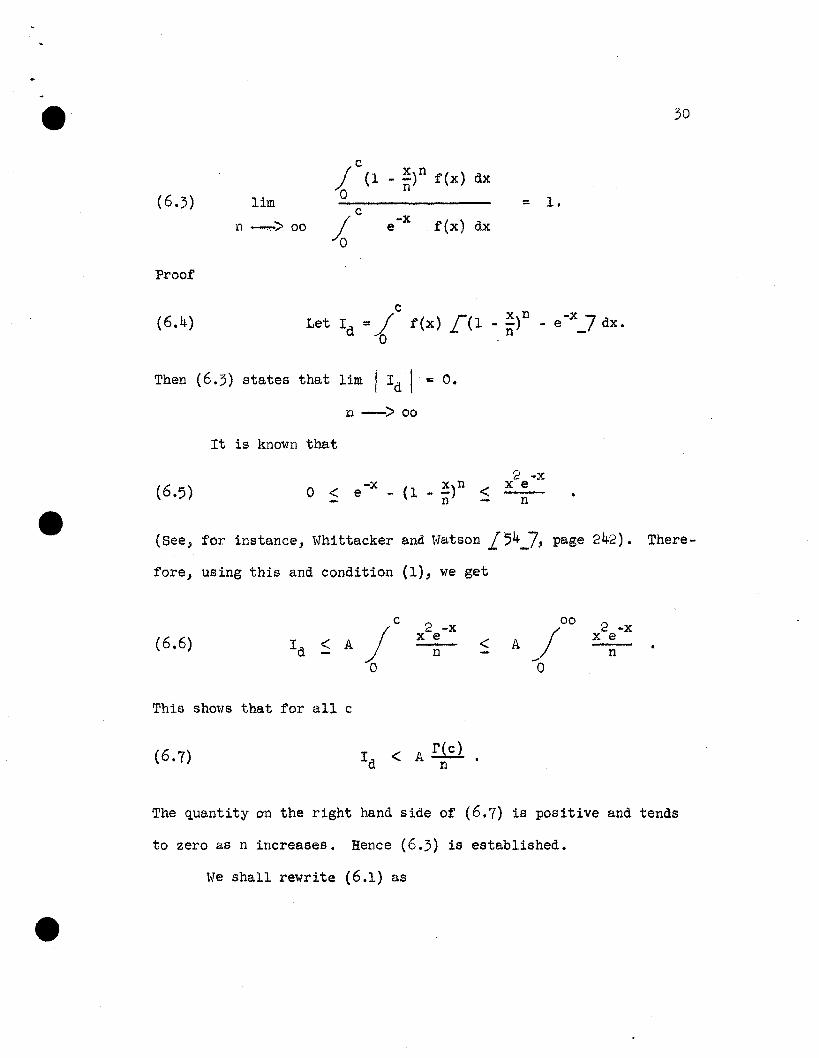
jC x n dx. (1 - -) f(x)

(6.3) limo n

1.=cn ~> 00

~-x f(x) dxe

Proof

c_ ~)n(6.4) Let Id =J f(x) F(1 -x 7- e _ dx.

0n

Then (6.3) states that lim I Id I = o.

n -> 00

It is known that

-x x)no < e - (1 - - <- n-

2 -xx en

(see, for instance, Whittacker and watson ~54_7, page 242). There­

fore, using this and condition (1), we get

(6.6)2 -xx e

n <2 -xx e

n

This shows that for all c

(6.7)

The quantity on the right hand side of (6.7) is positive and tends

to zero as n increases. Hence (6.3) is established.

We shall rewrite (6.1) as

31

(6.8)

and evaluate Ill' an asymptotic approximation to I l • This will be

followed by a Section on an upper bound to the error in using III

in place of I l •

To integrate with respect to m3

we first put

Thus

(6.l0)

Integration with respect to t~gives

(6.11) if

(6.12)

Making the transformation

2ml = Z cos 9,rj

m2 = z sin'- G,

we have

d{m1m2 )------- = 2z sin G cos G ;

d(z,9)

and so (6.11) becomes

(6.13) 2/z=o

rr/2

J9=0

n- -z p-l p-1p-l 2z e cos 9 sin 9 dzd9.

Integration with respect to 9 yields

(6.14)r(~)r(P;l)

I =----11 r(~)

r(~)r(~)

rep)

1

fz=o

n- 2Z p-l

e z dz;

and putting ~z = t we obtain the formc

Now for large n it is well known that

(6.16)

(6.17)

This further simplifies to

(6.18)

33

To be more exact we can write

n"2 co 00

(6.19) i -t p-l =j e-t t p - l dt -J e-t t p - 1 dt ,e t at

n~c.

and successive integration by parts shows that the right hand side

of (6.16) reduces to

(6.20)P 1 P 2n) - 1 n - p-l

r(p)-(2' n/2-2 n/2-"·'e e

p-lwhich can be written as r(p) - O(~)nh

e

as n tends to infinity,

p-1S. n~nce - n/2

e

tends to zero

(6.21) 4n(p-2)t (l+~) •nP n

We will show in Section 7 that t he error in taking III as

an approximation to the ~~irie 'of II is negligible 'in comparison to

the v.alue>;·of. Ii"'"

f It may be remarked in passiu~ that the integral occuring in

(6.11) could also be evaluated by usin g Dirichlet's formula ~54,

p. 258_7 namely

JJ ... f 0' -1t nn f(t11t2 •••+tn)dt1 •••dtn

(6.22)r(O'l) r(0'2)

-= r(Q'l + 0'2 +

nr. 0'.-1

i=l J.f(z)dz •

7 • An Upper Bound .!.£ ~rror.

In this section we shall consider the following problem:

How much error is committed by replacing

n-p-l2

by

in the tripe Dntegral (6.1) over the domain D1? We shall consider

two separate cases,

(A)

and

(B) >

and find an upper bound to error in both cases. 'The larger of these

35

shall ultimately be taken as the upper bound.

~ ! .. Let I d . dEmote the difference1

n-p-l2

I d will not decrease if in the factor ~l - ml - m2 + ml m2 - m~71

2 ml Tm2we omit m3

and replace ml m2 by (2 ). Making these changes, we get

The variable m3

can be integrated out by using the transforma-

tion

, ,

36

Using (6.22) in the double integral involved in (7.3), we get

(7.4)

1

r(p-l)r(E) j n-p-l ... !!. z2 2 p-1J.- z) 2 7'r(p ) . z (1 - 2" - e _ dz •

t=O

Replacing z/2 by t, (7.4) becomes

The expression

t=o

can be written as

(1 _ t)n-p-l -nt- e

(7.7) (1 - t)n-p-l _ e (n-p-l)t - (p+l)t• e ,

can be written as

(7.7) (1 - t)n-p-l _ e(n-p-1}t • e(p+l)t 1

which can further be written as

(P+1)t'+31 ••. 7- ;

and using the fact that 1 - Y~ eYwe find as a first approximation

that

(7.9) (1 - t)nl

_ ent < (1 _ t)nl

_ enlt + enlt (p+1)t •

This reduces to

(7.10)n' t 't(l-t) _en <en (p+l)t

by using the well known inequality

Using (7.10) in (7.5), we get

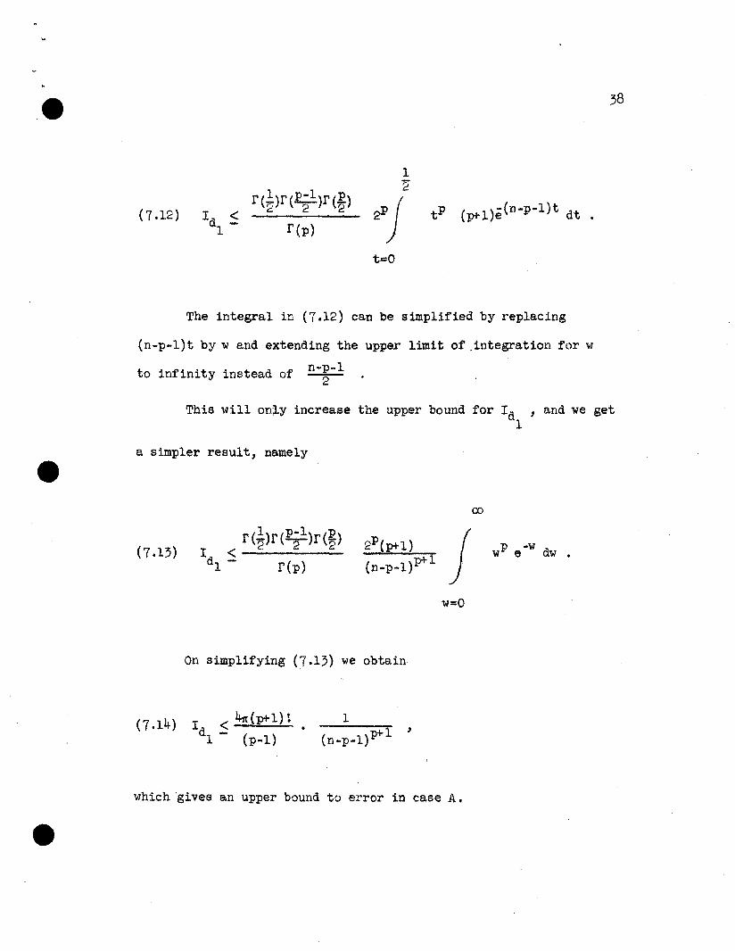
38

1

(7.12) iP~ t P (P+l)e(n-p-l)t dt .

t=o

The integral in (7.12) can be simplified by replacing

(n-p-1)t by wand extending the upper limit of ,integration for w

to infinity instead of n-~-l

This will on1y increase the upper bound for I d ,and we get1

a simpler result, namely

00

p -ww e dw.

w=o

On simplifying (7.13) we obtain

(7.14) I < 4n(p+l) td -1 (p-l)

1p+1 '(n-p-l)

which 'gives an upper bound to error in case A.

Case B. Now suppose

and let

39

Omitting the factor m1m2-m;, which is non-negative in the

domain of integration, one can write that

(7.16)

Integrating out m3

by the same transformation as was used

in Case A, we get

*(7.17) Id <1 jf

40

Using (6.22) on the dnuble integral involved in (7.17), we

obtain

1

r(~) reP;l) r(¥> )n n-p-l

* - - z -r(7.18) I d < zP-1L-e 2 _ (1-z) dll •1 - rep)

z=o

vJrite

n n-p-1 ~ n'z n'(7.19)

- 2'z(1 - z)

2 - 2 -2 2'e = e e (1 - z) ,

Where n' = n-p-l • Then

_ ~z n-p-1 n1z

(7.~0) e 2 _ (1 - z) 2 =e- ~L-1 pt1- ~Z +

C.

n f

'2(1 - z)

41

Since e-Y < 1 as a first approximation, we can write- ,

n n-p-1(7.21) ; 2

z_ (1 _ z) 2

and the use of (7.11) gives

n n-p-1- '2z 2

(7.22) e - (1 - z) ,

Replacing n I by n-p-1, and using this result in (7.18), we get

1

r(~)r(~)r(~)<

r(p) Iz=o

n-p-l--zpl-l n-p-l 2

z • -r e dz

n-p-1We put 2 z =w to get

n-p-12j wP<-l e-w dw

w=o

Extending the range of the integral to infinity and integrating, we

get

42

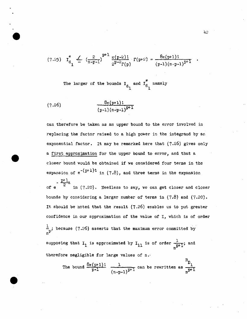
* / 2 p+l ( r), 8 (p+l)'4- ( ) :It p-c • r{p+2) = _..;.;,:rr~,--~'_~I dl n-p-l ';")p-2r (p) () , )pi- 1_ p-l {n,·p-l

*'The larger of the bounds I d and I d namely1 1

(7.26)

can therefore be taken as an upper bound to the error involved in

replacing the factor raised to a high power in the integrand by an

exponential factor. It may be remarked here that (7.26) gives only

a first approximation for the upper bound to error, and that a

closer bound would be obtained if we considered four terms in the

expansion of e-(p+l)t in (7.8), and three terms in the expansion

p+l-Tz

of e in (7.20). Needless to say, we can get closer and closer

bounds by considering a larger number of terms in (7.8) and (7.20).

It should be noted that the result (7.26) enables us to put greater

confidence in our approximation of the value of I, which is of order

1 .- ; because (7.26) asserts that the maximum error committed bynP

1supposing that 11 is approximated by III is of order p+l; andn

therefore negligible for large values of n.'

The bound 8:rr(p+l)lp-l

RD

1 can be rewritten as --!-(n_p_l)p+l np+l

by using the inequality 1 <~ for large n.(n_p_l)pi-l npi-l

Thus

(7. 27) "Error <R

Dl&c(pi-l)~ 1 1 II

p-l p+l = pi-l say.n n

As a result of the discussion in Sections 6 and 7 we can write

a formal proof of

Theorem 3.

Proof:

From the results of Sections 6 and 7 we can write

(7.28)

where I JD I < RD = l&c~rl)t and lim:. ( en ) = 01 . 1 P n ->00

Multiplying both sides of (7.28) by nP, and taking the limit as n

tends to infinity, of the right hand side in

4n(p-2) t + 4n(p-2) t en

the truth of Theorem 3 is established.

8. The integral over D2 •

(8.1)

44

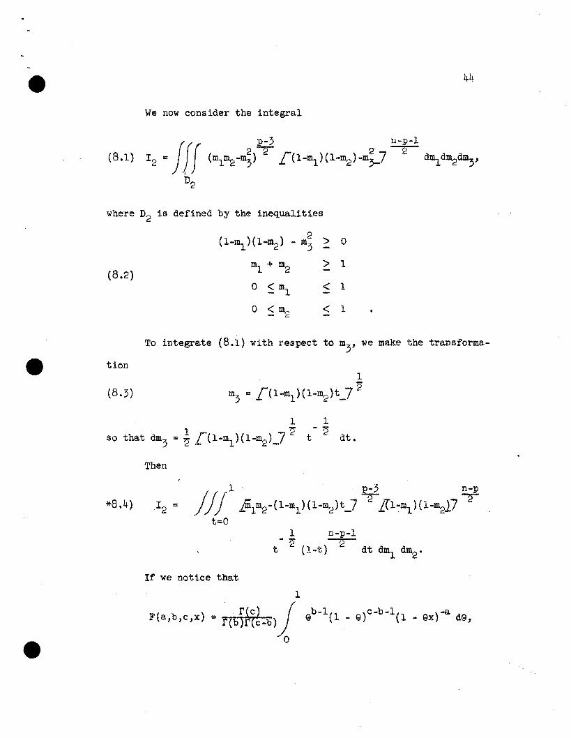
We now consider the integral

where D2 is defined by the inequalities

m1 + m2 > 1(8.2)

0 ~ m1 < 1-0 < m,_, < 1- c: -

To integrate (8.1) with respect to m3

, we make the transforma-

tion1

m3

= L(1-m1

)(1-m2 )t_7 2'

1

t- '2

dt.

Then

If we notice that

F(a,b,c,x)

1

=' f(c) j Gb-1{1 _ G)C-b-l(lf(b)f(c-b)

o

) -a• Gx dG,

provided that I x I < 1, we can rewrite (8.4) as

This step is justified by the fact that

(1-ml )( I-m2 )

m1m2

in the domain under consideration; except that on the surface of

the plane m1+ m2 = 1 we have an equality sign in (8.?). But the

omission of the point set determined by the plane m1+ m2 = 1 does

not alter the value of I r , since it forms a set of measure zero.c

(8.8) Since F(a,b,c,x) = 1 + ~b x + a~!;+l~~(b+l) 2x +

where, for the hypergeometric function involved in (8.6), we have

which the rth.term is 1of order -1 •r­n

Hence for asymptotic purposes

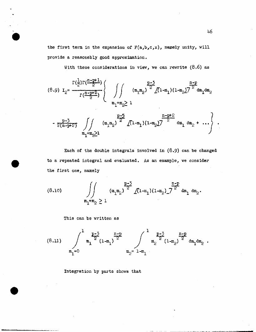
46

the first term in the expansion of F(a,b,c,x), namely unity, will

provide a reasonably good approxtmation.

With these considerations in view, we can rewrite (8.6) as

p-3- 2(n-p+2)

jf

..J·Each of the double integrals involved in (8.9) can be changed

to a repeated integral and evaluated. As an example, we consider

the first one, namely

(8.10)

This can be written as

(8.U)

m =01

m = I-m2 1

Integration by parts shows that

±'

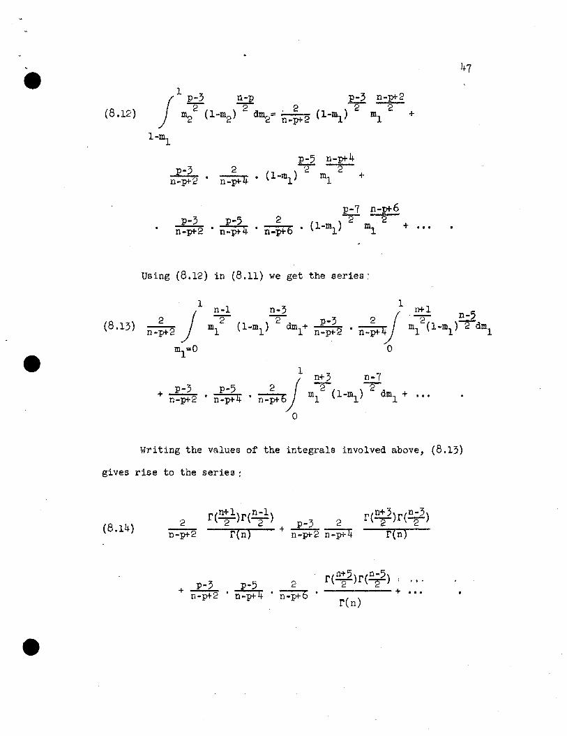
(8.12)

(8.13)

p-7 n-p+6p-3 p-5 2 2 2

n-p+2 • n-pt4 • n-p+6 • (1-m1) ~. + •••

Using (8.12) in (8.11) we get the series:

+~ p-5n-p+2 • n-pt4 •

Writing the values of the integrals involved above, (8.13)

gives rise to the series:

(8.14) 2n-p+2

r(~)r(~)r(n}

r(n+25)r(n

2-5} ;

p-3 p-5 2+ n-p+2 • n-pt4 • n-p+6 • ----- + •••

ren)

48

Similarly we can find the series expansions for the values

of the remaining double integrals involved in (8.9). Using (8.14)

as the value of (8.10), and similar values for the other integrals

(8.9) gives

(8.15) _ _ .....;.;.:J'(.l.(n;...-...=.p...r..)..;..t__12 =(n-2) t(n-p+2)2n-p

O( 1 )n32n

Use can be made of Stirling's approximation to the value of r(x),

namely

(8.l6)1

r(x) = e -x XX Z L-I + I~X + ...

Equation (8.15) shows that the principal term in the value of 12

is of order ~, where the actual value of,I2 differs from the<:::2--nn

n .

1principal term by terms which are of order~ and higher.n 2

9. An upper bound to the value of 12 ,

We can start from (8.6) and write

p-3 n-p r{!)r(n-p+I)2 2 2 2

(m1m) L(l-ml ) (l-m,,;)_7 --~~-~ ~ r(n-r 2 )

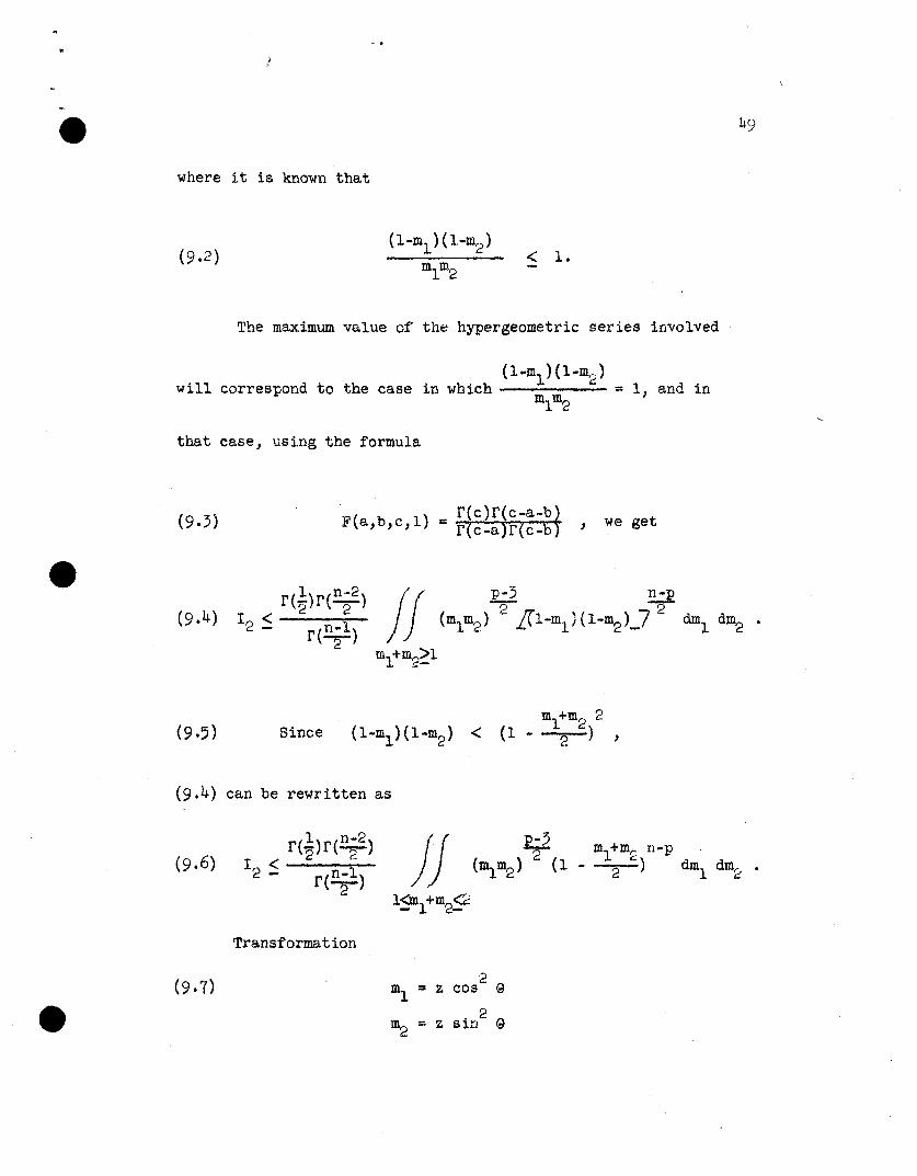
where it is known that

(9.2)(l-ml ) (1-m2 )

ml ffi2< L

The maximum value of the hypergeometric series involved

(l-ml )(1-m2 )will correspond to the case in which = 1 , and inml m2

that case, using the formula

, r (c )r (c -a -b)F(a,b,c,l) = r(c-a)r(c-b) , we get

Since

(9.4) can be rewritten as

j}Transformation

(9.7) 2ml = z cos 9

. 2 9m2 = Z SUI

reduces (9.6) to

r(~)r(n;2)I < 2 Co ~

2 - (n-l)rT

By using the formula

,J2 j; p-2 n-p p-2 p-2

z (l-~) sin 9 cos 9 d9 dz •

z=l 9=0

1f

)~

o

a-lsin 9

b-lcos G

1 r(~)r(~)d9 :0 -2 b

r(a~ )for

integration with respect to 9 , (9.8) reduces to

2

jz=l

p-2(1 z)n-p dz 2' z.

This inequality is the same as

(9.11)

1

j p-2n-pw (l-w) dw.

1w=-2

Observing that

/1'2

we have

p-2w

1

(l_w)n-p dw = 1 _ p-2 j wp - 3(1_w)n-ptl dw,2n-l(n_ptl) n-ptl

1'2

(9.12)f(P;l)r(P;l)

r(p-l) 2n-p1

(n-p+l)

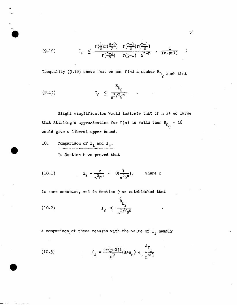
51

Inequality (9.12) shows that we can find a number RD such that2

Slight simplification would indicate that if n is so large

that Stirling's approximation for r(n) is valid then RD = 162

would give a liberal upper bound.

10. Comparison of I l and I2 .

In Section 8 we proved that

(10.1) where c

is some constant, and in Section 9 we established that

(10.2)

A comparison. of these results with the value of I l namely

(10.3)

where In is a certain constant less in absolute value than anotherI

known constant which is independent o~ n? ShOWB that

(10.4) limn-> 00

nThis statement follows from the obvious fact that 2 tends to

infinity more rapidly than nP where p is finite. This means

that the relative contribution of the domain D2 to the value of

the Integral I carried over D is negligible in the limit.

Theorem ()+).

Proof.

From (5.2) I = II + 12 , Usin.g (10.4) we have 1...-11 and

from theorem 3, Il~ ~(p-2)~ • Hence 4n(p-2)t which can alsop. p'

n n

be written as r(~)r(P;l)r(~) (~)p, is an asymptotic approximation

to the value of I.

As a further check of the correctness of our approximation

Ill' we can compare it with the exact value of the integral

referred to in Section 5. That value can be written as

(10.6) 4n(p-2)tIs = n(n-l) ••• (n-ptl)

where the subscript's' is for the author of the formula.

ing it with III written in (10.5), we have

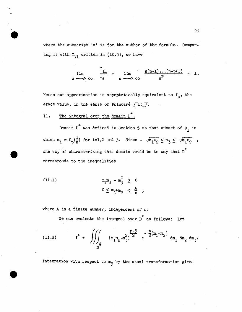
53

Compar-

limn -> 00

limn -> 00

n(n-l) ••• (n-p+l)

nP= 1.

Hence our approximation is asymptotically equivalent to Is' the

exact value, in the sense of Poincare ;-13 7.-. -

11. *The integral over the domain D .

*Domain D was defined in Section 5 as that subset of D1

in

which mi = Op(~) for 1=1,2 and 3. Since - Jm1m2 ~ m3 ~ vmlm2 '

*one way of characterizing this domain would be to say that D

corresponds to the inequalities

(11.1) 2 > 0ml m2 - m3

o ~ m1+m2 < An ,

where A is a finite number, independent of n.

*We can evaluate the integral over D as follows:-

Let

(11.2)

Integration with respect to m3

by the usual transformation gives

(11.3)* r(~)r(P;1)

I =----r(~)

Putting , and

and integrating out 9, we get

(11.4)

A

jnz=o

n- -zp-l 2z e dz

Substituting w for ~ z, (12.4) can be written as

(11.5 )

Thus

* r(~)r(~)r(~)I = r(p)

A2'

j p-l-ww e dw.

w=o

(11.6)* r(~)r(P;l)r(~) 2 P

I = r(p) (ii) £r(p)

00

j p-l -w 7w e dw_,

A2'

which on further simplification gives

(11. 7) I* = 4rc(p-2) t

nP

00

)A2'

p-l -ww e dw

55

Co~paring this vulue with the exact value Is we have

(n.8)*lim I = 1 ...,..-1-::'"'('-:"r - (p.,l)l

n -> 00 S

00

j p-l -ww e dw,

which is also = limn --> 00

*I

III

A:2

Since A might be a large number though not of the order of

.'1, tile term00

(11.9) 1 j p-l -w dw(p-l}l

w e

A2'

shall be small compared to 1; e.g., for p=3 and A=200, we get

1(p-l)l

00J wp - 1 e-w dw = e-LOOflo02+ 200 + 2_7 ,

A2

which will give a small fraction, and the fact is established that

*almost the whole of the density is concentrated in the domain D

near the origin. Equation (11.8) would indicate that even for A

*~s small as 10, and p =3 say D accounts for more than 99 per

cent of the density. In practice, however, A can be taken larger,

consistent with (11.1).

Another point needing clari£ication is the use of the

*exponential approximation over the domain .. Dl - D • At this

stage the justification is provided by the upper bound to error

n n-p-l- '2{m1+m2) 2 2

involved in using e instead of Ltl~ml)(I-m2)-m3-7

inside Dl , which was worked out 1n Section 7. The upper bound to

. ~1error for Dl was found to be -p+T. A closer bound can be worked

n- *out for the domain DI - D , and it can be shown that it is a

constant times the same upper bound multiplied by an integral of

This upper bound can be obtained by following the same

lines as those followed in Section 7.

12.

57

Summary of Chapter II.

In this chapter we have considered the asymptotic evalua-

tion of the integral

(12.1)1= ffi

D

where D is determined by the fact that both factors involved in

(12.1) are non-negative, and 0 < m. < 1, i=1,2. Two simplifica-- 1.-

tiona used in the evaluation of I are:

(1) D can be split up into two domains, Dl and D2, by the

plane ml+ m2=1. The contribution due to the domain D2, for

which ml+ m2 ~ 1 is negligible in the limit, in comparison with

that of Dl •

(2) The integral over Dl is evaluated by replacing the

n-p-l n( )2 2 - "2 m +m2

fa~tor ~(l-ml)(1-m2)-m3-7 by e 1 • The justification

for the approximation thus obtained is prOVided partly by the

probability order of the variables, and partly by the bounds to

error found SUbsequently.

With these simplifications it is proved that

(12.2) ,

and that the exact value of I can be written as

58

(12.3)

where the second term is the remaining contribution due to Dl ,

and the remaining terms give the integral over D2 • Bounds have

been found, (7.27), for JD and, (9.13), for the integral over1

D2 • These have been shown to be negligible as compared to the

principal term in the value of I, giving 4n(p-2)t as an asymptoticnP

apprOXimation to the value of I.

CHAPTER III

ON THE ASYMPTOTIC DISTRIBUTION OF 1rJALD'S CLPSSIFICATION

STAT1ST1C IN THE NULL CI1SE

1. Introduction.

We are dealing with the problem of classifying an individual

into one of two groups or popula~ions such that the information re-

garding the two populations is based on two samples of sizes Nl and

N2 respectively. One may be called upon to consider the following

three situations:

(A) Nl and N2 large,

(B) Nl + N2 or n( = Nl + N2 - 2) large,

(C) . Nl and N2 small.

The study of case A is equ~valent to the study of a linear

function of normal variates, that is, treating the statistic U, de-

fined in Chapter I, or the linear discriminant function, as normally

distributed with means and covariance matrix replaced by their sample

estimates to get the mean and variance of the approxtmating normal

distribution. This case has been completely exploited by several

workers in this field.

The results available in case C have been summarized in

Sections 4 and 5 of Chapter I. The difficulties involved in obtaining

the exact sampling distribution of

joint distribution of ~'~2 and m3

being substantial, it makes sense

61

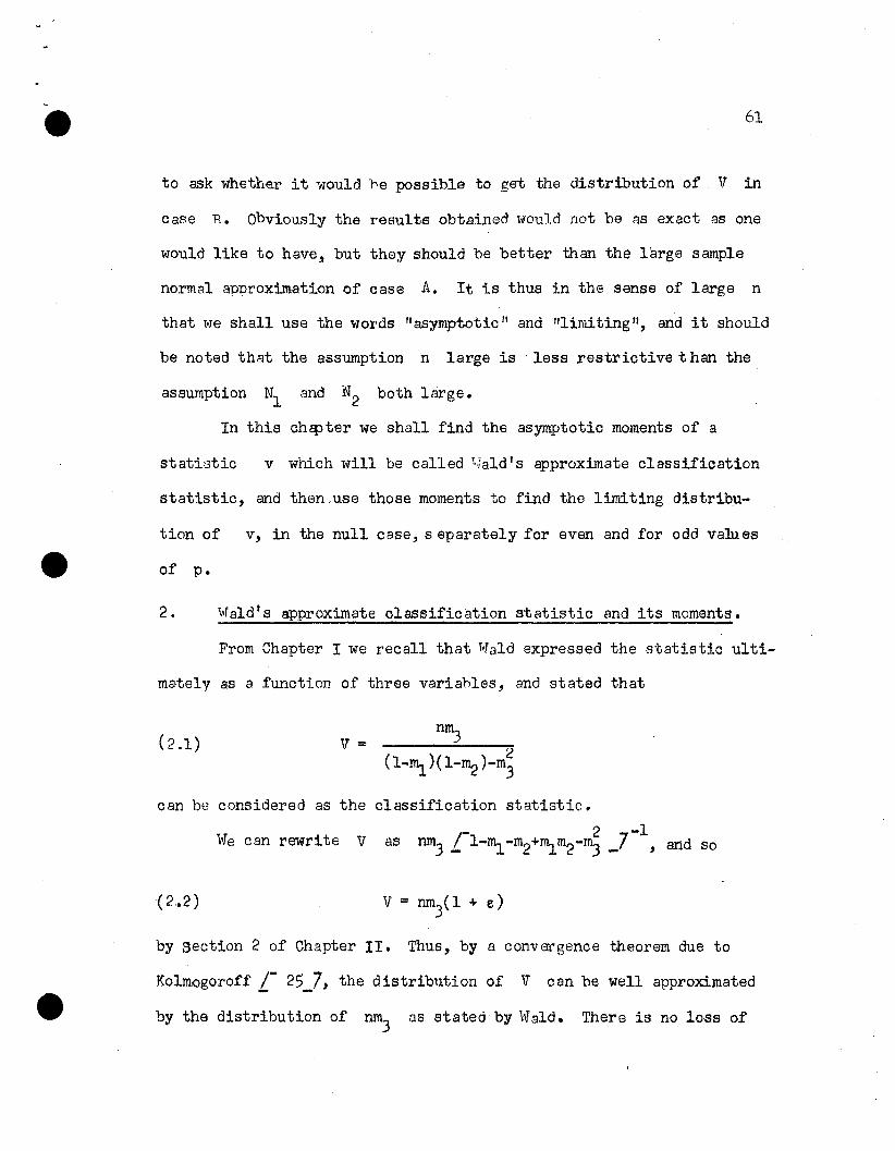
to ask wheth€.I' it would re possible to get the distribution of V in

case R. Obviously the results obtained would not be as exact as one

would like to have, but they should be better than the large sample

normal approximation of case A. It is thus in the sense of large n

that we shall use the words "asymptotic ll and "limiting", and it should

be noted that the assumption n large is less restrictive t han the

assumption Nl and N2

both large.

In this ch8pter we shall find the asymptotic moments of a

statistic v which will be called l.Jald' s approximate classification

statistic, and then,use those moments to find the limiting distribu-

tion of v, in the null case, separately for even and for odd valli es

of p.

2. Waldls approximate olassification statistic and its moments.

From Chapter I we recall that ~ald expressed the statistic ulti-

mately as a function of three variables, and stated that

Vo:

can be considered as the classification statistic.

by section 2 of Chapter II. Thus, by a convergence theorem due to

Kolmogoroff L- 25_7, the distribution of V can be well approximated

by the distribution of nm3

as stated by Waldo There is no loss of

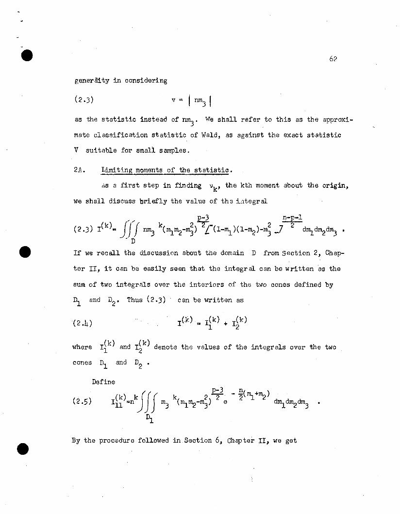
62

generaity in considering

as the statistic instead of nm3

. 1nTe shall refer to this as the approxi­

mate classification statistic ofWald, as against the exact statistic

V suitable for small samples.

2A. Limiting moments of the statistic.

riS a first step in finding 'Vk, the kth moment about the origin,

we shall discuss briefly the value of the integral

p-3 n-p-l

(2.3) I(k)= ]/'f nm3 k(~m2-m;) 2L(l-~)(1-m2)-m; _72-d~d~dm3 •

D

If we recall the discussion about the domain D from section 2, Chap-

ter II, it can be easily seen that the integral can be written as the

sum of two integrals over the interiors of the two cones defined by

Dl and D2• Thus (2.3) can be written as

(2.4)

where Iik) and I~k) denote the values of the integrals over the two

cones Dl and D2 •

Define

By the procedure followed in Section 6, Chcpter II, we get

63

(2.6)

which, for k :: 0, gives III of Chapter II.-

By following the methods of Section 7 and 9 of Chapter II, we

can show that the upper bound to the error in estimating Iik) by

Ii~) is of order ~+1' and an upper bound to the value of l~k) isn

Thus we can write

where

(2.8)

and

•

It should be noted that it is the upper bounds to, and not the

exact values of, In' and I D that are known; and to avoid dup1i-1 2

cation in their derivation, since they are obtained in exactly the

same way as similar bounds were found in Chapter II, we write the re-

suIts. They are

e.(2.10)

64

and

(~ .11)r(~)r(¥)r(I9)r(£~)n

k

I D2 ~ r(n+~-l)r(P_l) 2n+k- p(n_p+k+l)

It is easy to see from (2.7), (2.10) and (?ll) that

Inlim 1 = 0 , and

min I(k)n -> 00

I Dlim 2 = 0 ,

n -> 00 min r(k)

showing thereby' that In and In are negligible in comparison with1 2

the principal term in the value of I(k) •

Dividing (2.7) by III we get the expression for the asymptotic

moments, namely

(2.1?)

where

. nP+k2k+1

• (n"!J"iol)k+p+i

and

65

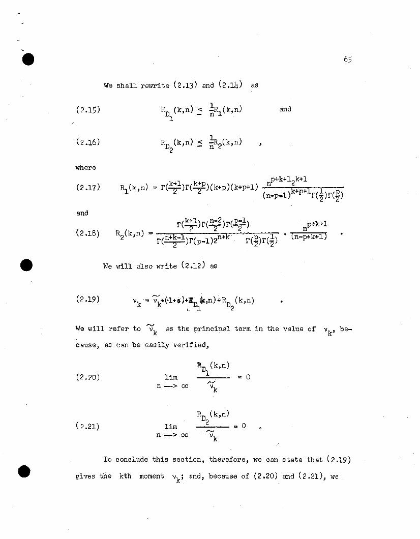
We shall rewrite (2.13) and (2.14) as

(? .15)

where

and

,

(2.17)

and

p+k+12k+l) k+l k+p ) ) n

Rl (k,n = r(T)r(T)(k+p (k+p+l k+p+l 1 P ,(n-p.l) r(2)r(~)

(2.18)

(2.19)

We will also write (2.12) as

p+k+ln

• (n-p+k+l)

•

•

We will refer to as the principal term in the value of V k, be-

cause, as can be easily verified,

(2.20)

(~ .21)

Rn (k,n)

lim 1 = 0,.../

n -> 00 vk

Rn (k,n)

lim 2 = 0 0"....

n -> 00 vk

To conclude this section, therefore, we can state that (2.19)

gives the kth moment vk; and, because of (2.20) and (2.21), we

6(

can write

(2.2?)

3. The asymptotic distribution of v ~ p = 2m •

In this section we shall find the asymptotic distribution .f

v for even values of p. By applying the general result we shall

also explicitly obtain the distribution for p = 2, 4 and 6.

Lemma 5.1.

and

r(~)r(£f:)

r(p-l)r(~)r(%)f or large n ,

Proo£':

The maximum value of n •• :l" 2 fQr n.> 2p + 2, and(n-p'-l) . '. -

r(%)r(~)~ ~ -1:, thr:rl)!or; th') ~th -of (3~1.) is a.,;,tablished.

To prove (3.2) we consider

r(n-2)2"

r n+k-l~

n+k2

p+k+ln

(n-p+k+l)

67

~+k

-. t th t 1 < 3 for 11 1 d 1 n 1We fh-au no e a n-p+k+l n a arga n; an s noe -2n+k- l <

for all large n

Lemma 5.2

The series

and < 1 for all n ~ 5, (3.2) follows.

and

are both convergent.

Proof:

Let uk denote the kth.term of the series. For the series

(3.5), we have

The ratio

(3.8)

Using Stirling's approximation to factorials, we have

..e 68

lim uuk := lim k~l (~).k -> 00 k+l k ->00 4

This simplifies to

lim uk "1. k _> 00 uk+1 = 2t

00

The ratio test stat es that the behavior of a series Z uk is deter­k=O

mined by the following formula:

,,

~ ::::::8:0:::::6:r1fo : : 1

I Series diverges if c < 1"-

formula shows that series (3.5) converges if

UkIf lim ---- = c

k ->00 ~+l

Application of this

(3.11)

t < 1/2.

Consider now the series (3.6). Since

k+lT o

r(~)r(¥)

r(p-l)r(~)r(~)

r(~)2

(3.12 )

limk -> 00

so that the series (3.6) converRes for all values of t. In particular,

1therefore, we can say that for t < ~ both the series (3.5) and

, 69e(3.6) are convergent.

In

.-vthere are three error terms if we approximate ~k by v k • Since the

other two are negligible in comparison to the upper bound to RD (k;n),1

it will be enough to consider the contri~ution of this to ¢(t) the

moment generating function of vk •

1ATe define

(3.16)

then by (2.19)

where e­n is the contribution due te other error terms and is easily

seen to be an infinitesimal of an order higher than that of ~.n

By virtue of Lemmas 1 and 2, we write (2.17) as

1 00 t k!0(t) - ¢(t)i < - Z --k

'Rl(k,n)~~

I I nk=O. n

uniformlV for all \ t I < ITO i 1< ~

Therefore by Paul Levy's theorem~9, p. 96_7

(3.20) ,

..tt 70

where F (v) denotes the sequence of cumulativa dist:'1 iliution functionsn

,,-.../

corresponding to ¢ (t) , and F(v) corresponds to ¢(t). Thuswen

have proved the following theorem:

Theorem ,.

If F (v)n is the sequence of cumulative distribution functions

corresponding to vk for large values of n, and F(v) is the distri­

bution function corresponding to 'Vk

, then given e, there exists

an Ne , ~uc~ that I F(v) - F(v) I < en

Theorem 6.

for n > Ne

When p, the numher of variables, is even, the asymptotic dis-

tribution of v is given by

mf(v)dy = Z b. f.(v) dv ,

j=l J J

where 2m = p,

1 j-l -j v>O'F[J) v e

(J .24) f. (v) = ,J 0 otherwise

and where the b .'s are suitable constants depending on m.J

Proof: Let p = 2m.

(J.26)

·e71

On exp!mding the right hand side of (3.26), we get

-::" =: (k+2m-2)(k+2m-4) ••• (k+4)(k+2) k~vk 2m-l • rrmJ

The moment generating function for the corresponding distribution is

given by

)

or

¢(t)00 tk.v~ i(T))k '

k=O 0

(3.28) z L (k+?m-2)(k+2m-4) ••. (k+4)(k+2)f(m) 2m- l

This can be rewritten as

( ¢~) . dm-1 k+m-1 k+m-2 d k+l k3.29) (t =c 1 -----1 Zt +c 2Zt +•••+c1 --dt L:t +cozt ,m- dtm- m-

where cOc1 ••• cm_1 are constants depending on m and these are ob­

tained by comparing the coefficients of like powers of k in (3.28)

and (3.29). The uniqueness of the solution for cOcl ••• cm_1 follows

from the fact that each of the expressions (3.28) and (3.29) consists

of a factor ~k multiplied by a polynomial of degree m-1 in k.

We can write (3.29) as

¢(t)m 00 m-i .

= Z c Z d (tk+m-~)i=l m-i k=O dtm- i

For fUrther simplification, we writeCDZ t k+m- i as

k=O

which can be expressed ast m- i-r:t' and the operations of summation

72

and differentiation can be interchanged in the region of convergence

of the series, namely I t I < 1 •

Also, since..,

and furtherm-i m-i-l 1 _ dm- i

d r- Z t A + /_ ( 1 )i 1 t - • I-tdtm- - A=l - - dtm-~

(,3.30 ) becomesm dm- i 1Z c. . (l-t)

i=l m-~ dtm- 1

This can be rewritten as

r....J

¢(t) = ~ c (m-i)ti=l m-i (l_t)m-i+l

::

~~

m c.Z m-J.

i=l (l_t)m-i+l

of

It is well known that 1 is the moment generating function(l-t )a

f (v) ::a

1 a-l-vrraJv e

o

v~O

v < O·

Hence we CAn write the distribution whose moment generating function

k

e73

m *f(v)dv = Xc. f .(v) dv. m-~ m-~~=l

This can" be expressed in a slightly better notation by writing j for

m-i. This completes the proof of theorem 6.

Special Cases.

(i) p = 2.

The kth moment is given by

tIVV =k

r(~)r(~)

rn,

which on simplification gives

(3.36)

,

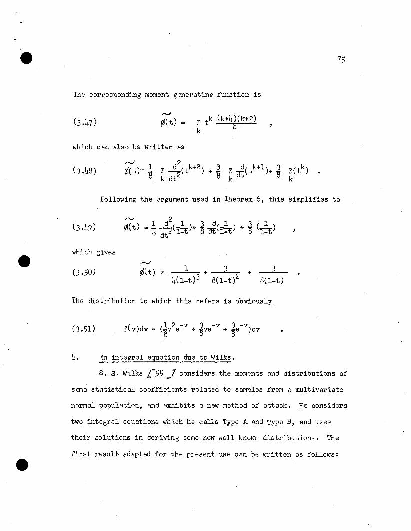
The corresponding moment generating function is

"r-.../ co¢(t) = l: t k

k=O

which can be written as

1= I-t

From (3.38) we conclude that

(ii) p = 4.

For p = 4 we have

if v ~ 0

otherwise

74

The mo~ent generating function for this, namely

~

¢(t) =: ,

can be rewritten as

,-..,.J

¢(t) =:d t k"'l tk

<;0 ( ) <;0(_)... -dt --;:;- + ... 2k t:. k

This on simplification becomes

The distribution of v is therefore given by

( ) l( -v -v)f v dv =: '2 ve + e dv

The moments in this case are given by

~

v =:k ,

which simplifies to

(k+4)(k+2) k!8

The corresponding moment generating function is

"""""¢(t) = ,

which can also be written as

Following the argument used in Theorem 6, this simplifies to

r.../

1 d2 1 1 {j 1(3.49) ¢( t) 3 ( 1== '8 ~(l-t)+ 8 crt(l-=t) + '8 'l-t)

dt

which givesr---.J

(J .,0) ¢(t) 1 + 3 + 3==

8(1_t)2•

4(1-t)3 8(1-t)

The distribution to which this refers is obviously

) ( (1 2 -v 3 -v 3-v(3.,1 f v)dv = '8v e + ave + 8e )dv

4. An integral equation due to Wilks.

S. S. Wilks L-" _7 considers the moments and distributions of

some statistical coefficients related to samples from a multivariate

normal population, and exhibits a new method of attack. He considers

two integral equations which he calls Type A and Type B, and uses

their solutions in deriving some now well known distributions. The

first result adapted for the present use can be written as follows:

If

(4.1)00

1 ,

whero k's and a's are real and positive and Band f(v) are

independent of k, then

f(v)

-82 8 2-1B v=f(al )r(a2)

v-x- -Bxe dx

The integral in (4.2) can be expressed in elementary functions when

al -82 is half of an odd integer; and this case, as we shall see later,

corresponds to the distribution of v defined in (2.3) for even

values of p. If, however, 81-a2 is an integer, the integral is

a Bessel function and this situation arises if p is odd. Before

using (4.2) in finding the distribution of v, we shall, for the sake

of completeness, add a note on Bessel functions.

5. A note on Bessel functions.

The equation

2 iw dw 2 2z ~ + Z dZ + (z -n ) = 0

dz

is called Bessel!s differential equ~ion of order n, and Bessel

functions are defined with reference to this equation. Its only

singularities are at z = 0 and z;: 00 c

~ solution in series of (5.1) near the origin enn be obtained

by supposing that w = ia.z:t

is a solution. It is found

77

that the discussion can be divided into four cases.

2i+l(a) n # i, n r ---2- where i stands for an integer.

In this case there are two independent solutions:

(5.2 )

where

J (z)n and J (z)

-n ,

J (z)n

00 (_l)r= i:

r=O r(r+l)r(n+r+l),

and is analytic for all values of z except possibly z ~ O. It

is called Bessel's function of the first kind.

(b) If n = i an integer,

J (z) and J (z) are two linearly dependant integralsn -n

satisfying the relation

J (z) = (_l)n J (z)-n n

In this case the solutions are

J (z) and Y (z)n n

where

•

n-1 ( -n+2rY (z) =J (z) log z _! i: n-r-lh (~)n n 2 r=O rt 2

1 00 (_l)r z n+2r- - E-· ('2) f¢(r) + ¢(n+r) 7,

2 r=O r(r+l)r(n+r+l) -

70

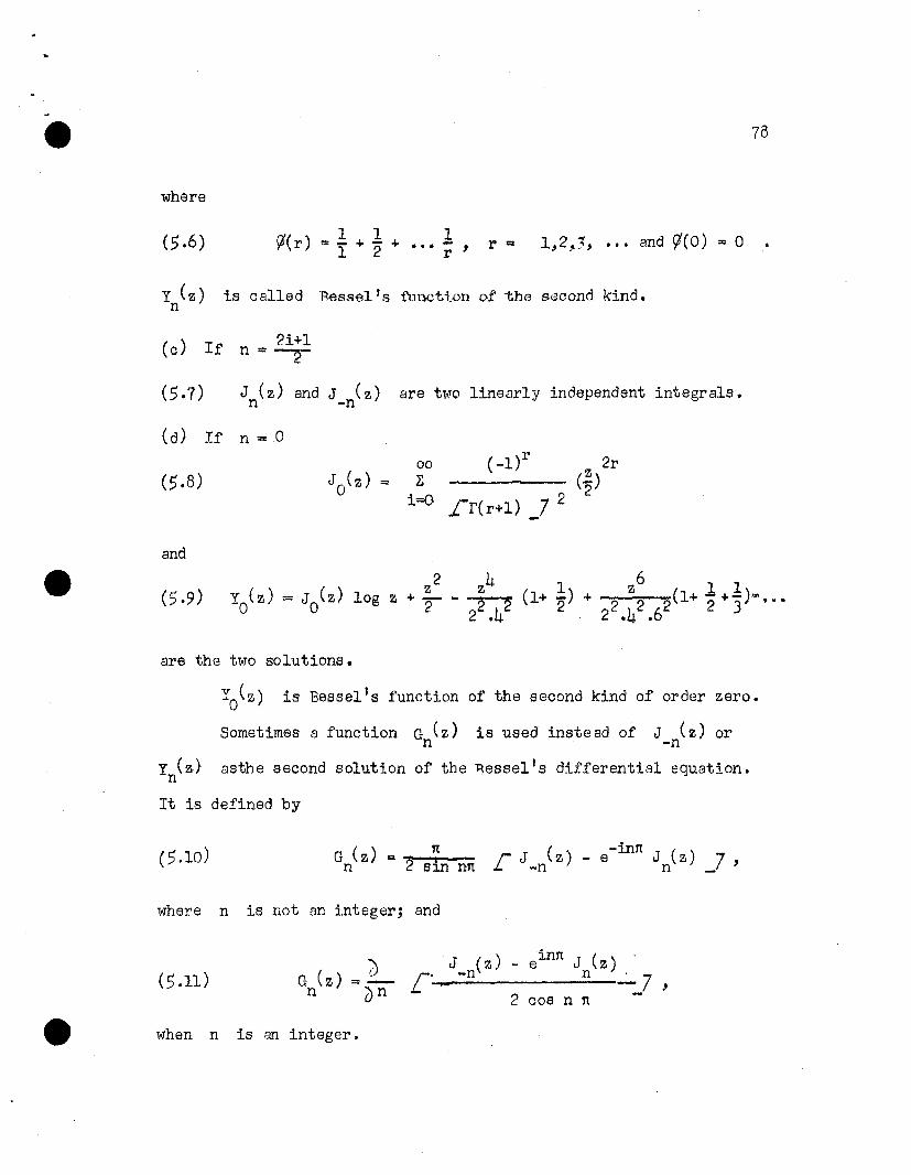
where

(5.6) rJ 1 1Y"(r) = - + - +1 21... r ' r = 1,2~;, •.• and 1/;(0) = 0

Y (z) is called "Ressel's functi.on of the second kind.n

J (z) and J (z) are two linearly independent integrals.n -n

and

00l:

i=O

2r(~)2

are the two solutions.

Yo(z) is Bessel's function of the second kind of order zero.

Sometimes a function G (z) is used instead of J (z) orn -nY (z) asthe second solution of the Bessel's differential equation.

n

It is defined by

G (z) ~ 2 ~ r J (z) - e-innJ (z)n SJJ1 nn .I- -n n _7 '

where n is not an integer; and

(5.11) G (z)n

J (z) - einn J (z) .L-' - -n n ...:.- 7 ,

2 cos n n -

when n is an integer.

tit 79

Ifwe put z = iv in (,.1), the result is

2 iwv -:-2 +

dv

dwv--dv

which is known as Bessel's transformed equation. Two solutions of

(,. .12), namely

I (v)n

00 1= l:

r=O r(r+l)r(n+r+l)

K (v)n

"" in G (iv) = __n__ L I_n(v) - In(v) _7 ,n 2 sin nn

are called respectively the modified Bessel functions of the first snd

second kinds of order n.

If n is a positive integer,

and

I (v) = I (v)-n n

,

K (v)n = lim

e -> 0•

6. Distribution of v for odd values of p .

In (2.2~) 'we proved that

(6.1)r(~)r(~)

r(~) r(~),.

which p-ives only the principiI term in the vaIu~ of ·Since we

,

60

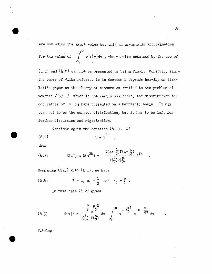
are not using the exact value but only an asymptotic approximation

- .. 00

for the valu~ of ~ vkf(v)dv, the results Dbtained by the use of

o

(4.1) and (4.2) can not be presented as being final. Moreover, since

the paper of Wilks referred to in Section 4 depends heavily on Stek-

loff's paper on the theory of ~losure as applied to the problem of

moments ~47 _7, which is not easily available, the distribution for

odd values of p is here presented on a heuristic basis. It may

turn out to be the correct distribution, but it has to be left for

further discussion and rigorization.

Consider again the equation (6.1). If

2u=:v

then

(6.3)r(k+ ~)r(k+ ~)

r(~)r(~)•

(6.4)

Comparing (,.3) with (4.1), we have

B =: 4, al :; % and 8 2 =: ~ •

In this case (4.2) gives

(6.5)

Putting

p p-2- '2 2

f(u)du= 4 u dur(~) r(~)

00

1p+l u

- 2"" -x- 4ix e dx

(6.6) 2u ::: V and p::: 2m + 1 ,

81

we get

00

.jo

-m-lx e

2-(x+ ix)

dx

According to '~Tatson £52, p. 183 _i the integral

v200 -x- 4X~ x-m- l e dx , has been studied by Poisson, Glaisher, Kapteyn

·0

and others. The result stated in Watson is

(6.8) lvmjOOK (v) => -(-)m 2 2

o

2-(x+ +-::)

-m-l L.j..l'..x e dx

This reduces the distribution of v to the form

Putting m = 0, 1, 2, ••• iQ this, we get the distribution of v for

p :::r 1, 3, 5, •..•

7. The use of a differential equation in the evaluation of an

integral.

In Section 6 we found that

p+l- --n"x c

v2-x- 4X

e dx ,

82

where p is the number of variates in the underlying normal distri-

butiolTS •

1\ known teclmique for l:::\rE1luating

ro

¢( v) :: io

p+l v2- -r -x-17X

x e dx

is as follows:

¢(v) ::

p+l 00

2T j

odz •

Now we define

00

rev) = io

1 2 ·2..l.. - "?(z t ;)p-2 - zz e dz >., .

wherev2;O.

dz

12 2- -(z + ;)

2· z1- ezP

co

Y'<v) = -v1

Since the conditions for differentiation under the integral

sign are satisfied, we differentiate \Vev) with respect to v and

get

Similarly

dz

1 2 i- "'2(z + 2)

L- 1 z 7d 1~ EI z:= - ep-~ _ p-lz z

Now 2l( 2 "l/.)

-"'2'z.~z

e dz

12 2... -(z + ..!..)

2 2z

83

00

o

which is equal to zero identically therefore, using this identity we

obtain, from (7.4), (7.5) and (7.6), the following differential equa-

tion

The value of riC v) can be found by using the solution of th1.s and the

fact thatI p+l

¢( v) = _ if (v) • 2~ •v

8. The asymptotic distribution of v for even and odd values of p.

We shall, in this section, derive the distributions of v again

by starting with the result,

(8.1)OJ

12p+l v

.. 2' -x- wex e dx , and

by evaluating the integral involved by the help of (7.8) and (7.9).

We divide the discussion into two cases.

Case A. p := 2, 4, •.•

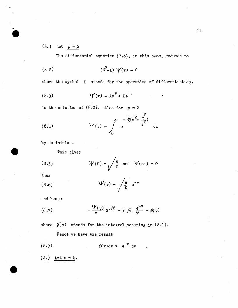
Let p:: 2

The differential equation (7.8), in this case, reduces to

where the symbol D stands for the operation of differ6ntiatio~.

(8 .3) \.( (v) = Ae v + Be- v

84

is the solution of

by definition.

(8.2). Also for p = 2

1 2 200 - '2(z + ..;)

"\f(v)=j e Z

odz

This gives

(8.5)

Thus

(8.6)

and hence

;; \//\V (0):: /"2 and T (00) = 0V

II/() 1;-vi v "'V 2 e

where ~(v) stands for the integral occuring in (801).

Hence we have the result

f( v)dv =-ve dv •

·e 85

Here

(8.9)00

'(v) ~.1 dz ,

but from

(8.10 )

(8.4) and (8.6)1 2 2

00 - ~(Z + .;) ~'

1 z n -v° e dv =V ~ e

Differentiating both sides of (8.10) with respact' to v and dividing

by -v, we get

(8.11)

Thus

-ve-v

(8.12)

Hence from (8.1)

() 1( -v -v)f v dv = 2' e + ve dv

Here

(8.14)

12 200 - -( z + v2)

y (v) .... i ~ e 2 Z dz •

° z

Using the reasoning of example 2, we get

(8.15 ) '!f'ev) ~Ii-v -vve +e

•

86

Therefore

(8.16)

This value substituted in (8.9) gives the' follow.l.~ distribution for

p "" 6.-v -v 2-v

f(v) dv = )8 +)VS +v e dv

The process can obviously be carried on to get the distribu-

tion of v for all even values of p.

Case B. p ::: ), 5, ...

(Bl ) Let p = 3·

The differential equation satisfied by ~(v) in this case

reduces to

C8.17) ,

which is the modified Bessel equation of order zero, and is satisfied

by

Therefore

(8.18)

But

¢Cv) •

(8.19 )

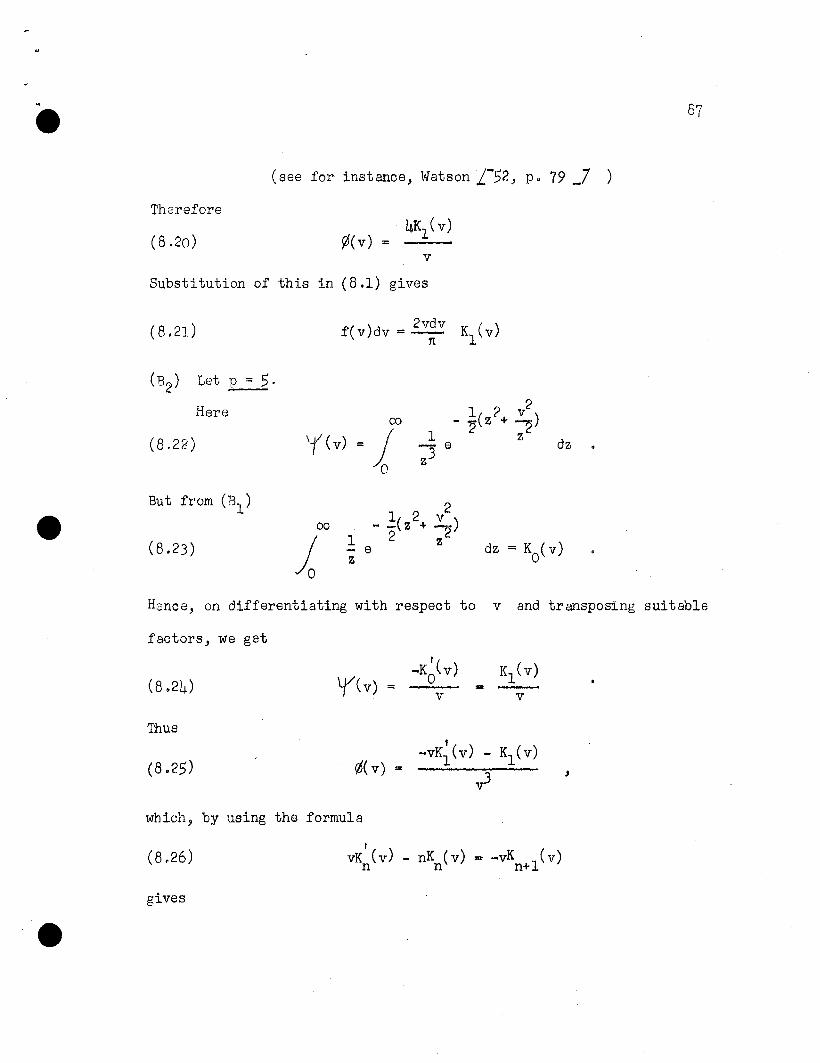
87

(see for instance, Watson i-52, p. 79 _7 )Therefore

Substitution of this in (8.1) gives

(8.21)

(B2) Let P "" 5.

Here

(8.22)co

'rev) = jo

dz

(8.23)00

la1 2 2

- -( z + v2

)1 2 Z- ez

Hence, on differentiating with respect to v and transposing suitable

factors, we getI·

(8.24) 'rev)-Ko(V) Kl(V)

= => -v v

Thusf

(8.25) ¢( v)-vKl (v) - Kl ev)

""v3

,

which, by using the formula

(8.26)

gives

I

vK (v) - nK (v) => -vK ( v)n n n+l

88

( 8.27)

and consequently

as the distribution for p = 5 .

This nrocess can obviously be continued to obtain the asymp-

totic distribution of v for all odd values of p.

This section also shows that we get the same distribution of

v for p = 2m by the two methods, namely

(1) The use of the moment generating function }

(2) The application of the integral equation given in Section 4.

9. Note on the construction of tables.

Case A (When p = 2m)

The distribution of v in this case is

(9.1)m

f( v) dv "" Z b. f . (v) dvj=l J J

where

f . (v)=J

(1 .i-l -j\ rmV"' e

L 0

v > 0

otherwise

00

j f( v)dv can

x

The evaluation of the integrals of the type

and where the b.'s are constants which can be found for Any givenJ

integral value of m.

..e 89

?obviously be made to depend on tal)les of YJ- distribution with even

degrees of freedom. For illustration it will be enough to consider

the cases when p = 2 and p = 4.

and the substitution

f(v)dv= e-vdv

)~2v = - shows that

2

p( v > l!) = p( 'X 2 > a)2

which gives the method of tabulat ing areas for the distribution of v.

In thi.s particular case it may be more convenient to use the

tables of exponential function.

Here

() l( -v -v)f. v dv = '2 G + ve dv

Putting,.'x-2

v =~. this becomes

The two frequency functions inside the square brackets are~2 fre-

quency functions for two and four degrees of freedom. Consider the

following table giving tail areas for these distributions.

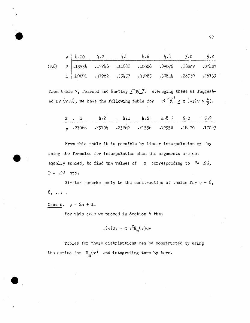
2 .13534 .12246 .11080 .10026

4 i .40601 .37962 .35457 .33085t

.30844 .28730 .26739

..

V i 4.00 4.2 4.4 4.8

.09072

5.0

.08209

90

5.2

.07427

from table 7, Pearson and Hartley ~35_7o Averaging these as suggest-

'\/' xed by (9.5), we have the following table for p(,.... ~ x )=p( v > '2.)'

x .' 4

p .27068

. 4~4

.25104 .23269

4.6 '.

.21556 .19958 ,,18470 .17083

From this table it is possible by linear interpolation or by

using the formulae for interpolation when the arguments are not

equally spaced, to find thp. values of x corresponding to p= .25,

p ,.. .20 '3tc.

Similar remarks anuly to the construction of tables for p = 6,

8, •.• :)

Case B. P = 2m + 1.

For this CAse we proved in Section 6 that

TQbles for these distributions can be constructed by using

the series for K (v) and integrating term by term.m

10.

91

Sma~ary of Chapter III.

In this chapter we have discussed the distribution of v = Inm3

\

for large values of no The kth moment E(vk) is found in Section 3

by following the methods of integration developed in Chapter 110 These

moments have been used in finding the asymptotic distribution of v

for even values of p by the help of the corresponding moment generat-

ing function. For obtaining the large sample distribution of v for

odd values of p, use has been made of an integral equation due to

S. S. Hilks.

CHAPTER IV

AN ASYMPTOTIC SFRIES EXPANSION FOR THE DISTRIBUTION OF

1. Introduction.

w = IN THE NULL CASE

Harter L-18_7 has obtained the distribution of m3

as a double

series by starting with the joint distribution of ml , m2 and m3

of

ihTald in the special case when P i = 0 = t i' which we call the null

case, and which has been the subject ~f our discussion in the pre-

ceeding chapters. The series obtained by Harter would present diffi-

culti9s in practical applications, since in any practical situation

the number n, which is determined by the sizes of the two samples,

will not be very small. For large n the investigator wishes to use

that distribution of m3

in which the ratio of each term after the

-1 Ifirst to the preceeding term is of order ntis also obvious

that the main point in getting such a series 1s to obtain terms beyond

the first. Of these, however, the second and third approximations are

of chief interest and are doubtless easier to calculate than any of

those of higher order. 'Recause of these considerations in this chapter

we shall obtain the first three terms in the distribution of w = tm31

as an asympt~tic series. For the first a~proximation the constant ef

integration will be found, and the method of finding the tail areas

for the construction of tables will also be discussed.

It might be noted that the statistic w is ~ times the statis­n

tic v defined in Chapter II. Towards the end we shall also compare

93

the result. of this chapter with that of Chapter III.

2. An asymntotic series for the distributioq.

i~e consider the joint probability distribution of ml , m2 and

w, which is the same as the probability distribution of ml , m2 and m3

except for the constant of integration because

Let C denote the constant of integration. Then

(2.1)

The region of integration is determined by

2> 0m1m2-w

~ -

(1-ml )(1-m2)-w2

> 0(2.?) D =: ,

l~~ > 0

1 .:: m2 > 0

which alsft determines the range 1 variate Im31o < w < - for the w = .- - 2

To integrate with respect to m1 and m2

, we shall keen w

fixed, and put m =: x -+ y and m =: X - Y . This gives1 2

p-3 n-p-l( ) ( 2 2 2 ?/-( 2 2 2 22.3 f x,y.w)d;ldydw "" ?C(r -y -w) _ x-I) -y -w _7 d::i::dydw

For fixed w, the two expressions in the brackets in f(x,y,w)

are zero on hyperbolas in the (x,y)-plane. Mnreover x + y = 0 and

222x - y = 0 are the asymptotes of x -y =w , and x + y - 1 ~ 0 and

x - y - 1 = 0 are the asymptotes of the hyoer~ola (x _ 1)2 _ y2 = w2 .

The region of integration f~r x and y is thus the area encl~sed

by the two hyperbolas and is sh~wn in the figure on the adjoining page.

The coordinates of the points of 1ntersection A and B €Jf

the two hyperbQlas are1

1 1 2 2'A = £ - (I. - w) _72' 4

11 1 2 '2

B = f -, -(- - w) 724-

The probability distribution of w will be given by the following

double integral:

/1 2V. '4 -w

r(w)dw ~ 20 I.J /1 2Y=-14 -w

r:-32 2 2-"'2

(x -y -w )

(2.5)

n-l"-l

i -ex )? 2 2 7 2- 1 -y - w _

Put

p-32" = r

dx dy dw •

..e

'-IJ

x-l+y=O

96

and

n-p-l.-.,~ = q

2

AI 1 th 't· t / 2 2 bso rep ace e POS1 1ve roo VY +w Y a

To perform the integration with respect to x, we shall suppose

Y to he constant. Using (2.5) and by noticing the symmetry of the

inte?rand in y, we can write (2.4) a~ f(w)dw, where

(2,6)

/1

JIt'T;

f(m) = 4c •

-y=O

Let

2-w. I-a

Jx=a

( 2 2)rL-( )2 2 7qx -a r-l -a _ dx dy •

This transformation sets UP a one-to-one correspondence between the

values of x and the values of v. Furthermore, as x increases from

a t~ I-a, v increases monotonically from zero to one.

From (2.7) we have the following:

(2.8)

x = 1 -r.2 2/ a +(l-?a)(l-v)

2v + •••

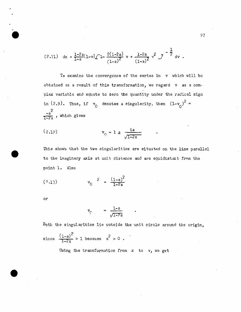
·e

(2.11)

97

11-2a 2 7 - "2v + --.....~ v _ dv •

(l-a)

To examine the convergence of the series in v which will be

obtained as a result of this transformation, we regard v as a com-

plex variable and equate to zero the quantity under the radical sign

in (2.9). Thus, if va denotes a singularity, then

2-a~ , which givesJ..-ca

2(l-v) =a

v = 1 .±oia

/1-2a

This shows that the two singularities are situated on the line parallel

to the imaginary axis at unit distance and are equidistant from the

point 1. Also

or

2

=

( l_a)21-2a

l-a

JRa

Both the singularities lie outside the unit circle around the origin,

since(1_a)21-2a > 1 because

2a > a .

Using the transformation from x to v, we get

.e 98

1

(1-2a) r (

(l_a?+l a via

v +

We write (2.14) after expanding the last two binomials, but

omitting terms involving cubes and hipher powers of v since they

will not affect the first three t8rms of the desired asymptotic series.

This gives

/1 2v'4- w

/I

.Jy=O

(1_2a)q+r+l ra

( l_a)r+l

1J' vr (1_v)2q+l

v-=O

v +

) 22~. r 2 L- (r-l (l-~a+a )

2(1-a) 4a

. 2 la( 1-2a L7v + ••• j

/-1 1-2a (a

2+4a-2)(1-2a) 2 7_ + )2 v - ->----~.-;..r.4----- v • .• _ dv dy

(l-a ?(l-a)•

,

e 99

This can further be reduced to

(a2+4a-2)(1-28) r(1-3a+a

2)(1-2a) 7 "}

2(I-a)4 + )3 - + co. dv dy

2a(1-a

Integration with respect to v after replacing q and r by

their values in terms of n and p, gives

(2.17)

1 n-2 p-3E+ ( 2 T

f(w)=2 {' C ) 11-2a) ~

-" ?Y (I-a)

r(n-p+l)r(9)

( 2n-p+l)r 2

2 ( 2)21+ /- 1-2a + (p-3)(1-3a+a ) 7 p-l +/- p-3)(p-5)(1-3a+a- (l_a)2 4a(l-a) - 2n-p+l - 32a~(I-a)2

l

(p-3)a(I-2a)).j.(I_a)2

<l+4a-2)(1-2a) (P-3)(1-3a+a2)(1-2a) 7.

2(I-a)4 + 2a(l-a)3 -

~-- ----~-~~-

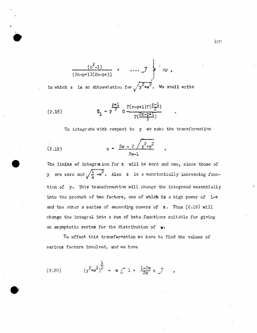
is an abbreviation

2(n -1)

(2n-p+l)(2n-p+3)

in which a

+ .... J }'rlY ,

,);,.....2--~2

for V Y +w • We shall write

(2.18)

To integr8t€ with respect to y we make the transformation

(2.19) Z =1222w _ 2 / yc.+wc.

2w-l

The limits C)f integret ion for z will be zero and one, since those of

;r-:;yare zero and Vu -w. Also z is a monotonically increasing func-

tion of y. This transformation will change the integrand essentially

into the product of two factors, one of which is a high power of l-z

and the other a series of ascending powers of z. Thus (2.19) will

change the integral into a sum of beta functions suitable for giving

an asymptotic series for the distribution of W.

To effect this transformation we have to find the values of

various factors involved, and we hAve

(??O) ,

(2.21) 2 2 2 /­y+w=w_l+ 1-2w-z+W

101

1

( 2 2)2 ( r 1-2w 71- y +w = 1 - w)_ 1 - 2(1-w) z _ ,

(2.23)

1222 ( )1-2(y + w) = 1 - 2w)(1 - z ,

and

dydZ

1(1-2w)2/-2w -+- (1-2w)z 7

1 1

2z2L-4w+(1-2W)z_72..,

The singularities zl" z2 and z3 of the resulting series in z

are determined by the equations

(2.26)

and

respectively.

1-2wl+-W z=O

l-2w1 - 2C1-w) z = 0

l-2w1 + ""'1'iW z = 0

..

102

From these we have

(2.28)

(2.?9)

and

2wzl =

~w-l

z2 =2(1-w)1-2w

(2.30) Z ::::3

4w~

Since the range of w is from 0 to ~, we find from the above three

equations

(2.31)

(2.32)

and

(2.33)

-00 < zl < 0

2 < z2 < 00

-00 < z3 < 0

In otherwords, two of the singularities lie on the negative half ef

the real axis and one on the positive side in the z ?lane. To be

ablato get a convergent series in z we have to make sure that these

singularities do not lie in the unit circle around the origin. To

examine this, we proceed to find the range of values of w for which

z > l-

(i) Izll > 1 if ?w 1 if > 11-2w > or w Ii

( ii) Iz2! > 1 if 2f:2:) >1 or if 2> 1 which is true

( iii) Iz31 > 1 if 4w > 1 if 11-2w or w > '6

..

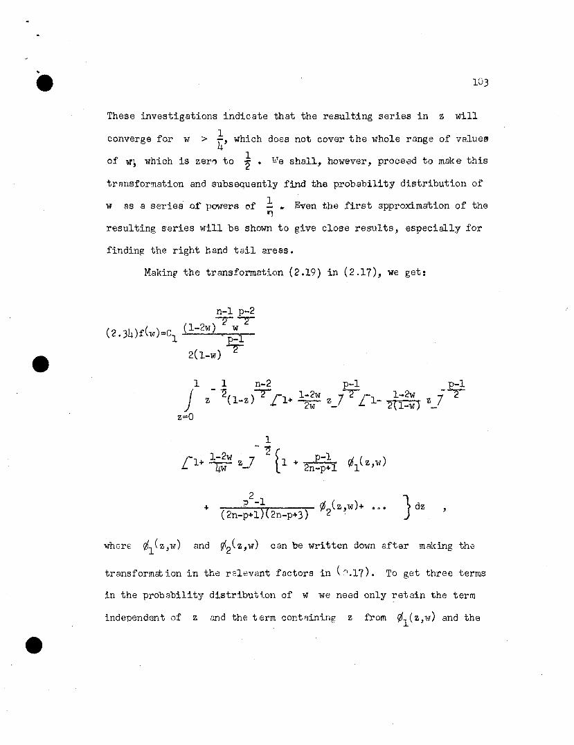
These investigations indicate that the resulting series in z will

converge for w

of vt~ which is

> ~, which1zerr, to 2' •

does not cover the whole range of values

We shall, however, proceed to make this

transformation and subsequently find the probability distribution of

w as a series o:f powers of ! .. Even the first approximaftion of thefl

resulting series will be shown to give close results, especially for

finding the right hand tail areas.

Makinr the transformation (2.19) in (2.17), we get:

n-l p-2--r --r

(2.34)f(w)=C1 (1-2w) -P~l

2(1-w) 2""

1 1 n-2 p~l p-l

)" - ~(l )7'1 1-2w 72 '1 1-2w z 7- 2

z -z ~ + -zw- Z_ L - 2(1-w)z=o

1- '2

L-l+ 14w2w z_7 ~1 + p-l rI. ( )l 2n-po4ol \iiI z,w

+ ,

where ~l(z,w) and ¢2(z'w) can be written down after making the

transformation in the r21evant factors in ('">017). To get three terms

in the probability distributi.on of w we need only retain the term

independent of z and the term containinR z from ¢l(z,w) and the

..

..e 104

term independent of z from ¢2(z,w).

If we retain only those terms in the various expansions involved

in (2.34) which contribute to the first three terms of the desired

series, we get

n-l p-222

(2.35) few) = CL (1-2w) wl p-l

22(1-w)

1. 1 n-2j z -2(1_z)2£1+ (P-l)~;-2W) z+

z=O

( ) ( 2 2Ll+ p-l)(1-2w z+ P -1)(1-2w) 2

4 (l-w) 3:?(1-w)2 z +

/- l-2w 3(1-2w)2 21-~z - z +

- oW l28w2

p-l (L- l-2w + (P-3)(1-3w+w2

) 72n-p+l (1_w)2 4w(1-w) -

2/-(1-2w) l-2w

+ ---..".-+- (1_w)3 (1_w)2

)

(p-3)w(1-2w) (w2+4w-?)(1-2w) + (P-3)(1-3w+w2)(1-2w)4tl~w)~ _. 2(1-w)4 2w(1-w)3

Further simplification gives

+ ...J} dz •

..

105

n-l p-222= c (1-2w) w

1 p-l. 22(1-w)

1 1 n-2

J -2(1 )2[1 /- (p-l)(1-2w) . (p-l)(1-2w)z -z +_. 4w ~ 4(1-w)

z=o

1-2w 7 /-(P-l)(P-3)(1-2W)2 (p2_1)(1_2w)2- ~- Z+ 2- + 2

oW ' - 32w 32(1-w)

2 2 2 )23(1-2w) (p-l) (1-2w) (p-l)(1-2w- 128w2"~ 16w(1-w) - 32w(1-w)

) p-l /- 7 p2_1 L- 7~l + 2n-p+l _ A + Bz+ ...... + (2n-p+l)(2n-p+3) E+ ..._ + ] dz .'

where A, Band E are functions of w, and are known explicitly from

(2.35). For the sake ~f brevity we write this as

n-l p-~27

few) :: c(l-2w) w1 p-l

2"2(1-w)

1 1 n-2j z - 2(1_Z) 2L-l+Alz+l\Z?+ .. ,_7,

z=o

I ( p-l - .' .:r>~~l:; -E+ }ll+2n-p+l LA+Bz+ •• ,_7+ (2n-p+-l)(2n-p+3) L .' "_7+ ,., dz.

..e 106

The integral involved in this can be writt.en ~

1 1 n-2

(2.38) J z- 2(1_z)-2- (l+L- ~n~;~l A+Al

z_7 +

z=o

,

where the terms in curly brackets are arranged in three blocks accord-

ing as they contribute to first, second and third approximations.

Integrating with respect to z, we have from these

p-l A + -!- A 72n-p+l n+l l-

2

/- (p -l)E p-l (

+ _ (2n-p+l)(2n-p+3) + (2n-p+l)(n+l) .B+AA1)

where

A =1-2w

"2(l-w)

(p-3) (1_3w+w2)

+ 4w(1-w) ,

..eB = (1-2w)~ _ 1-2w ~ (P-3)(4w4-11w2+7W- 1)

(1_w)3 (1_w)2 8w2(1_w)2 j

A = (p-1)(1-2w) + (p-1)(1-2w) 1~2w1 4w 4(I-w) - -aw'

107

B = (p-1)(P-3)(1-2w)2 + Ip2~1)(1-1W)2-1 32w2 32(1-w)2

and

(p_1)(1_2w)232w(1-w)

)o-1)(1-2w)232w2 .

2 2 2E = (P-3)~p-5)(~-3W+W) _ .(P-3)w(1-2wl _ (w +4w-2)(1-2w)32w (l-w) 4(1-w)2 2(1-W)4

+ (P-3)(1-3w+w2)(1-2w)2w(1-w)3

Furthermore,

1 1 ( P_1)-1 1 p-l (1)2n-p+l = 2ii 1-~ = "2!i + 7'"2

4+ 0 3 '

n n

•

III 1n+1 = - - -~ + 0(-)

n n n3 ,

111(

",.;;;, = --""l'\' + 0(-) ,2n-p+1)(2n-p+3) 4nc n3

1..,------ .(2n-p+1)( n+l) + O(~)

n,

··e1

(n+3)(n+l)1 0(1:...)... "2 + 3n n

,

108

Using these in (2.39), the first three termg of the series

can be written as follows:

n-l p-2 p-l(2.40) f(w)dw "" It (1_2w)-r w "'"T(l_w) 2[1+ fj- E? A + A

1_7 +

Explicit expressions for the first, second and third approximations

can be written by substituting the values of A, B, Al

, ~2 and E from

(2.39). This series can be written as

(2.41) few) = Kfl(w)L-l+ ~A(W)+ ~~(w)+ O(~) _7 ,n n

1and is such that the ratio of each term to the preceeding term is -,n

and is the desired asymptotic series.

3, The constant of integration for the first approximation.

The first approximation to the distribution of w is

p-2 p-l n-l( ) ~()- -,- ~ -1

(3.1) f w = KlW l-w (1-2w) + O(n )

where 1O<w<-.- - 2

The cons tant of integr ation can be found by start-

ing with the constant of integration of the triple integral found in

..

109

Chapter II or directly by integration from (3.1) as follows:

(J.2 ) 1Kl

=

~2 p-2 p-l n-l~ W~(l-W}- ~(1-2w)~ dw

o

Let 1-2w = y, then

. 1 n-l E~ p-11 1·) 2"" 2 -2(3.3) K = - y (l-y) (l+y) dy1 ~ 0 .

By comparin? with the hypergcometric integral, we can write

(3.4)

(3.5)

we get

1 1 r(~)r(~)Kl = Ii r(n+~+l)

Using the formula

F( a, b,c,x)

(U-l n+1 n+p+l )F T' 2' 2,-1

(l_x)-a F(a,c-b,c, -Xl)x-

(J.6 )

Since the third coefficient in thenypergeometric series involved is

large, the value of the series can be approximated by 1 for large n,

that is

and we can write

(p-l p n+p+l 1lim F "'2 ' "2' 2 '"2) = 1

n ->00,

(3-.8 ) 1- P2 "2

r(~)r(~)

r(n+~+l)

IQa

Using Stirling's approximation, it can be further simplified tl'l

,

giving approxim~tely the constant of integration in the first aPDroxi-

mation.

4. The tail areas for the first approximation.

Let

The transformation y = l-2w reduces it to

I-x

)

n-l p-2 ~-lT T --'2

y (l-y) (l+y) dy

a

This is the kind of integral we will have to evaluate for finding prob­

abilities of the tyoe pew > ~).

W2 write the integral involved in (4.2) as:

t n-l

(L~.3) IJ,(t) = J ""2 'A( ) dyy y ,0

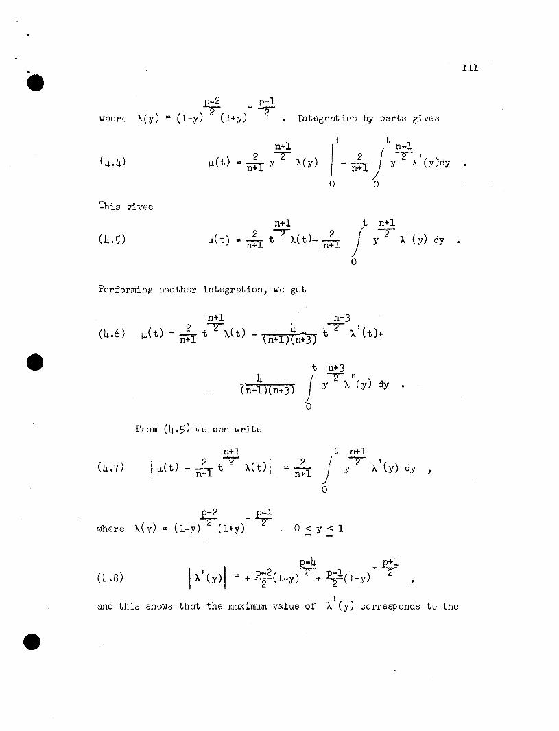
III

where~ - E;l

A(Y) = (l-y) (l+y) 2 • Integrati(m by parts gives

n+l2 T

~(t) = n~l Y A(Y)

t t n-l2) 2 1

- n+l y A (y)dy

o 0

This I!ives

n+l2 ""2 ) 2

~(t) =~ t A(t - ~n+J. n+J.

t n+l

j 2 1Y A (y)

o

dy •

Performing another integration, we get

(4.6)n+3

4-r I(n+l)(n;3) t A (t)+

dy •jt ~ rl

y A (y)

o

__ 4(n+l)(n+3)

From (4.5) we can write

n+l2 T I1f.l.(t)-n+It A(t)

t n+l2 j T 1= ---1 y A (y) dy ,n+

o

1~here ),,(y)

p-2 p-l""T - T

= (l-y) (l+y) o < y < 1- -

(4.8)

I

and this shows that the maximum value of A (y) corresponds to the

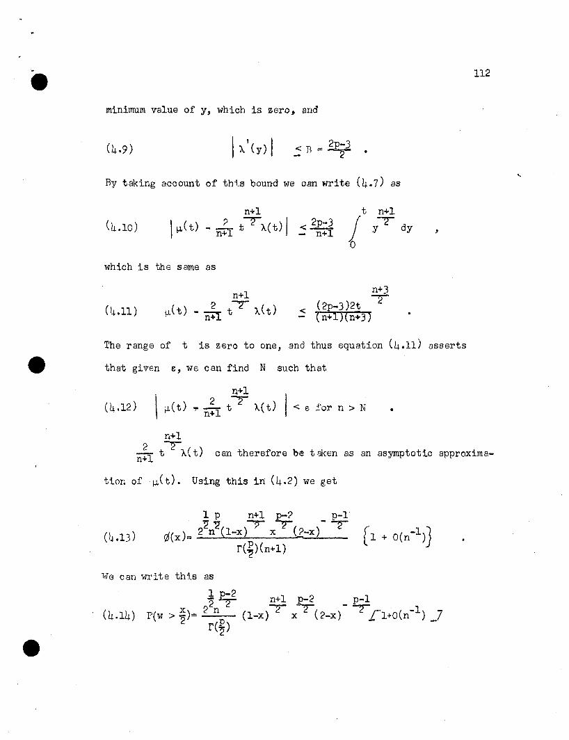
112

minimum value of y, which is zero, and

< B := 2p-3- 2 •

By taking account of thi.s bound we can write (4.7) as

t n+l

j y2 dy

o,

which is the same as

(4.11)

n+1

~(t) - 21

t2 A(t)n+

n+32(2p-3)2t

< tn+1)(n+3)

The range of t is zero to one, and thus equation (4.11) asserts

that given &, we can find N such that

n+1

~(t) ~ ~ t~ A(t) I< e for n > Nn+l •

n+l2 T---1 t A(t) can therefore be taken as an asymptotic approxima­n+

tion of ~(t). Using this in (4.2) we get

1 P n+1 p-? p-12"2 ? T -7

¢(x)= 2 n (l-x) x <..~-x) [1 + o(n-1)]r(~) (n+1)

lATe can write th1.s as

1 p-2'2 2 n+1 p-2 p-1. ( x) 2 n T T( - T 14.14) pew > '2 = (l-x) x 2-x) ..C1+0(n-) 7

r(~)

..

113

which provides a formula suitable for finding the tail areas of the

5. Comparison with the results of Chapter II~.

We have shown in this chapter that if we omit terms of order}n

p-2 p-l n-lT -T 2

f(w)dw :=: C w (l-w) (1-2w) dw

To get the corresponding first approximation for the distribution of

the statistic v= , we put vw = - in this, and getn

p-2 p-l n-lC T -T 2-"2

f( v)dv = - v (1- !) (1- 2) dvp n nn

Since

and

(1.i )

n-llim(l _ ~)2

nn-->oo

-ve

p-llim (1- !)-T

nn-->oo

1

.. 1

= 1

,

we can write (5.2) as2 .

B.:... -v2 ;- 1f( v) dv = Const. v e . dv _ 1 + OCii) _7 ,

which st3tes that for large n) v is approximately distributed as

~ 114

2'}./2 where the 'Y---2 has p degrees of freedom.

This is not in agreement with the probability distribution ~f

v obtained in Chapter III, and this discrepancy can be easily explained

by the fact that the convergence of the eeriee'tn ··.. ·"~n (20-38)0' ::.

W3S not guaranteed for the whole region of w. It was seen on pages

101-103, that convergence of the series in z· from which we obtained

f(w) by integration would be obtained only if 1w > '4. However, it

appears that the two distributions would give close results if we are

interested in the tail areas. As an illustration we shall find apnroxi-

mately the 5 % point for p = 4 by the results of the two chapters.

F~ample. To find x such that P(v > x) = .05 in the two

cases

(1)

From table 7, L~35_7w6 have the following values fQr the prob­

3bility integral of the ~ 2-distribution.

Giving p( ,,--2 > 1--2 )- 0

'. 2~C1 7.8 8.0 8.2 8.4 8.6 8.8

d.f

2 .02024 .01832 .01657 .01500 .01357 .012::>8

4 .09919 .09158 .0845? .07798 .07191 .06630

Sum .11943 .10990 .10109 .09298 .08·548 .07858

1 .05972 .05495 .°5055 .04649 .04274 .03929"2 Sum

j

• 115

The last row gives probabilities .f the type 'p(2v > )Lg) or

p(v > vO) say, and shows that approximately p(v > 4.1) = .05 if we

use (1). Also from the same table we find that p(v > 3.9) = .05 if

we use (2).

6. Summary of Chapter IV.

In this chapter we have considered the problem of obtai.. ning an

asymptotic series for the distribution of w = m3

by starting with

the joint distribution of ml , ~ and m3

in the null case. The de­

sired distribution is obtained by integrating out ml and m2 over

a lana shaped region enclosed by the two hyperboles ml m2 =w2(a con­

stant) = (1-~)(1-m2)' To perform the two integrations, one with

respect to x = ~ + m2 and the other with respect to y =~ - m2

we have, at each stage~ regarded the other varia~les as constants and

found a transformation which changes to integrand into a function of

the form b i~ci(l - z) z, where b is a large number, and where zi

varies from zero to one. This leads us to a result of the type

few) = K L-fl(w) + ~f2(w)+ ~ f3

(W)+ ••• _7.n

First three terms of the asymptotic series have been obtained in

this ma~~er. For the first approximation we have also found the con-

stant of integration, and discussed the method of finding tail areas.

In Section 5 we have compared the results of this chapter with

those of Chapter III.

• CHAPTER V

THE APPLICATION OF TCHEBYCHEFF-MARKOFF INEQUALITIES

TO A SPECIAL CASE

1. Introduction.

This chapter will be confined to the discussion of the

special case p = J and Nl+ N2 = 20. In this case, starting

from the joint distribution of rol' m2 and mJ , we shall find the

moments of the exact statistic V. These moments will then be

used in setting up bounds to probabilities of the type P(V ~ ~)

by the use of some investigations due to Tchebycheff and Markoff

~48_7, ~49_7. This will provide, on the one hand, some exact

results of some importance for this case, and on the other hand

illustrate what can be done when the first few moments of an

unknown distribution are known.

2 • The integral over Dl •

As before, we shall denote by 11 and 12 the integrals

over Dl and D2 • Thus

(2.1)

Expanding the integral by the use of the binomial theorem, we

get

•(2.2) Iff

117

Each of the integrals in this sum can be calculated by

1/2first putting m,= (m1m2t) to integrate with respect to t,

then following the procedure of section 6, Ctnapter II. The result

is

(2.') II = rr. I 901

16 +1

11 + 12 +• 32 . ,0 • 48 • 88 •

1 1• 8 +

116 • 98 • 12 • 11 . l} + ;2 • 26 • 88 32 • 1,0 • 64 • 6

1 + 1 7+ ~1~28n--·~3~2-·~1~2~0---.~8 256. 128 • 16 • 17 - ,

which is therefore the integral over Dl •

3. The integral over D2 •

This has been found exactly in Chapter II} but anindepen-

dent derivation based on geometrical considerations could be

given here.

IffThe value of 12 ~e want will be obtained by putting n = 18.

•(3.2)

Then

In (3.1) put u = (m1 + m2) //2

and v = (m1 • m2) /.j2 .

Then let v = r cos Q

and J2m3

= z = r sin G •

11:

1(3.3) I = -

2 !2/

./2 Ju2+ 2(1- 12 u) .2n 2 2 n-4

/ j ur 2·(1- V2u+ ; ) 2d9drdu .

1· 9=0u=- r=O

J2Integration with respect to G and r is immediate, and yields'

{2

(3.4) 1 2 = 2n1' J1

12

2 n-2.Tr5 u 2

(1- V2 u + 2) du.

Puttingu = 02x and integrating we obtain,I = 'J(

2 (n_1)(n_2)2n-3

and for n = 18, it reduces to

•(3.6) 1t1

2;=: --..-;.;.---=-......

17 • 16 • 215

IIJ

4. The integral over D.

The value of I, the integral over D, is

(4.1) = 18 • 17 . 4

5 • Moments of V.

The kth moment ~ is given by :

Due to the symmetry of f(m~m2m3) the joint density function of

kml ,m2 and m3

in m3,E(V ) = 0 f~r odd values of k.

Putting k = 2, 4 and 6 io(5.1) and integrating as in

Section 2, we get the following moments:

(5.2)

We knm'1 that V >

~2 = 6.5571637176,

~4 = 459.6304942728,

~6 = 25661.8~65464

since V equals n m3

divided by a

quantity which cannot exceed one, and in fact remains less than

one inside D. Thus, since the range of 18m3

is from -9 to 9,

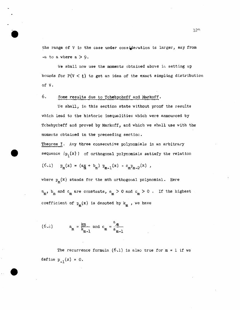
• 12 f1

the range of V in the case under cons~eration is larger, say from

-a to a where a > 9.

We shall now use the moments obtained above iI, setting up

bounds for P(V < ~) to get an idea of the exact simpling distribution

of V.

6. Some results due to Tchebycheff and Markoff.

We shall, in this section state without proof the results

which lead to the historic inequalities which were announced by

Tchebycheff and proved by Markoff, and which we shall use with the

moments obtained in the preceeding sectioD.

Theorem I. Any three consecutive polynomials in an arbitrary

sequence fp.(x) 1 of orthogonal polynomials satisfy the relation1

(6.1) p (x) = (ax + b ) p lex) - c p 2(x) ,m m m m- m m-

where p (x) stands for the mth orthogonal polynomial. Herem

a ,b and c are constants, a > 0 and c > O. If the highestm m m m m

coefficient of P (x) is denoted by k ,we havem m

<:lkm d .ma = -k- an c = ...-

m m-l m a m_1

The recurrence formula (6.1) is also true form = 1 if we

define p_1(x) = O.

• 121

Theorem II. The roots of the equation p (x) = 0 , where p (x) ism m

the orthogonal polynomial of degree m associated with the weight

function cx(x) on the interval (a,b) Jare all real and distinct;

and all of them lie in the range of definition of the polynomials.

Theorem III. If

oo(x) ,z-x

where o(x) is the weight function of the system of polynomials, then

wls satisfy the same relation (6.1) as the pIS, though with different

initial conditions.

Definition. Let

(6.4)m p.

= r. _1_

i=l z-C i,

where ~ (z) is or degree m-l in z, whereas p (z) is of degree m.m m

The c i are the roots of Pm(z) = O. Suppose a < cl < c2 ••• < cm

< b,

where (a,b) is the range of the basic function Q(x).

called the Christoffel numbers.

Then p. are1

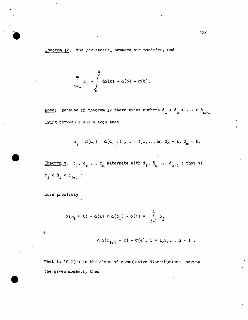
•Theorem IV. The Christoffel numbers are positive, and

b

m J~ Pi = ~(x) =a(~) - a(a).i=l

a

122

Note: Because of theorem IV there exist numbers dl < d2 < ... < dm_l

lying between a and b such that

Theorem V. ••• d 1m- that is

more precisely

iL P

J.

j:::l

<a(c i +l - 0) - a(a), i::: 1,2, ... m - 1 •

That is if F(x) is the class of cummulative distributions having

the given moments, then

•c

ij dF(x)

a

. d i

< J dF(x) =

a

C i +1

~, p. <J dF(x)j=l J

a

123

7. Application of Tchebycheff-Markoff Theorems to this Example.

We have the following matrix of the moments of the distribution

studied in this chapter:

\-lO III 1-12 113 114

III 1l'2 113 114 115

112 113 114 115 116

113 114 115 116 117'"

=

0 6.557163716 0 459.·630494 16.557163716 0 459.6}0494 0

0 459.630494 0 256661.8465

459.630494 0 256661.8465 0 ,/"

in which all four principal diagonel matrices are positive definite.

Let

(7.1)

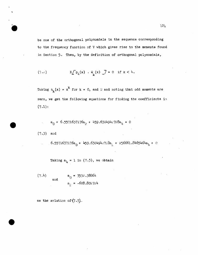
• 124

be one of the orthogonal polynomials in the sequence corresponding

to the frequency function of V which gives rise to the moments found

in Section 5. Then, by the definition of orthogonal polynomials,

(f.e:)

Taking Gk(x) = xk for k = 0, and 2 and noting that odd moments are

zero, we get the following e~uations for finding the coefficients lD

(7.1):

(7.3) and

6.5571637176ao + 459 .63049427~8a;;; + 256661.8465464a4 + 0

Taking a4 = 1 in (7.3), we obtain

(7.4)and

ao = 353"2.38864

ar- = -608.80~7~4c:

as the solution of'7.3).

•Thus

l~

Solving P4(x) = 0 we get the following four values of x ,

arranged in increasing order of magnitude

Now the function ~4(z) can be found using its definition

given in (6.2~, which gives

(7.7)4 4 2 2

(z - x· ) + B2 (Z. - x )~4,(Z) =E ;

x z - x

and, using (5.2) and (7.4), this becomes

(7.8)

The Christoffel Numbers.

The Christoffel numbers as defined in Section 6 are the

numbers p. given by1

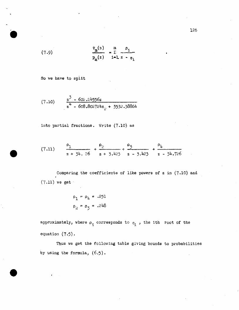
• 126

m Pi= L: -i=l z - 01

So we have to split

(7.10)

into partial fractions. Write (7.10) as

3.423(7.11)

z + 34. 26+

p~) P3----+~---z + 3.423 z-

+z - 34.726

Comparing the coefficients of like powers of z in (7.10) and

(7.11) we get

Pl = P4 = .251

pr = P3 = .248Co

approximately, where p. corresponds to c. , the ith root of the1 1

equation (7.5).

Thus we get the following table giVing bounds to probabilities

by using the formula, (6.5).

• 127

Table 7.12

Limits for E

s < -34.726

-34.726 < S ~ -3.423

-3.423 < s:: 3.423

3.423 < S ~ 34.726

34.726 < ~

Bounds for

p(v < ~) = p

P < .251

o < P < .499

.251 < P S .747

.499 < P .:s 1

.747<P~1

It can be seen that the bounds given above are far from

being close. For obtaining bounds which are sufficiently close

and therefore useful we would have to calculate a large number of

moments. The labor involved in finding enough moments, and pro­

ceeding with subsequent investigation based on those, however, is

prohibitive of any such invGstigation in these pages.

CHAPI'ER VI

NON-NULL CASE

1. Introduction.

This chapter will be devoted to the study of the non-null case.

In these first few sections W3 will consider the joint probability

distribution of ~, m2 and mJ

given by Sitgreaves L-45_7. This dis­

tribution corresponds to the statistic

and has been obtained under the restriction that the mean vectors of

the two populations are proportional to each other. For large n we

shall convert this into a different form. Some of the difficulties inI

proceeding beyond that point will also be discussed.

The next section will deal with the distribution of

,2: ij C - x ) for the "" 1, and the assumption thatU "" 2: s zi Yj

case P oni j

j

h is large so that 2 can be replaced by 2 This assumDtion re-s er .duces U to the product of two normal variates whose distribution is

known; see for instance ~2 7, /-8 7 and /27 7. It has not been- - - --possible to extend this to the case p >,1.

In Section 7 of this ch9Pter we have exemplified the differential

method which was quite popular with statisticians a few years ago. The

illustration deals with the finding of approximat ions to the mean and

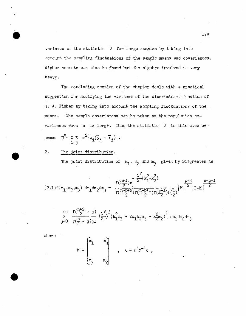
·e 129

variance of the statistic U for laIrge sam!lles by tcking into

account the sampling fluctuations of the sampl~ means and covariances.

Higher moments can also be found but the algebra involved is very

heavy.

The concluding section of the chapter deals with a practical

suggestion for modifying the variance of the discriminant function of

R. A. Fisher by taking into account the sampling fluctuations of the

means. The sample covariances can be taken as the population co-

variances when n is large. Thus the statistic U in this case be-

comes

2. The joint distribution.

The joint distribution of ml

, ~ and m3

given by Sitgreaves is

where

00

~

j=O

fC n+2 .) 2'-2+ J A. J 2C-) Ck In..

fCE + j)jl 2 1 ~2

.....

~ m3

M= ' -1, A. => 5 Z 0.9

l.....m3m2

130

and ~5 and k20 are the mean vectors.

Using the not8tion of the confluent hypergeometric series,

we can write (2.1) - as

p-3 n-p-l

1M! 3" II-~/f I 2

where

F( n+2 p x)2' -" ,

The function F(a,c,x) is also written as ¢(a,c,x) or as IFI(a,c,x),

and is known as the confluent hypergeometric function.

3. Notes for reference on confluent hypergeometric functions.

Consider the hypergeometric series

( ) + a.b z + a(a+l)(b.)(b+l) z2F a,b,c,z = I c c(c+~ ~ -I- •••• ,

in which we suppose that both a and c are positive. F(a,b,c~~)

gives a power series with b as the radius of convergence. It

defines an analytic function with singularities at 0, b, and 00. The

limiting case of this series as b --> 00 defines an entire function

whose singularity at 00 is the confluence of two singularities of

F(a,b,c,~) and which can be written as

131

( ) ax af a+l~ x2(3.2) F a,c,X = 1 + cIT + c 0+1 ~ + •••

It satisfies the confluent hypergeometric equation'

(3.3)d2 ' d

x J. + (c - x) .Ql - ay = 0dx2 dn

Accordi.ng to Bateman L-4_7, the asymptotic behavior of ¢fa~x)

as a --> 00 has been discussed by Perron, Tricomi and Taylor.

An asymptotic form of F uniformly valid in the neighborhood of x=O

given by Taylor is

1 c x 1

(3~4) F(a,c,x) = r(c)(Kx)2 - 2 e2 Jc

_l

L-2(Kx)2 _7+ O(-1

K )

where c and Kx are bounded, and K c/2 - 8, and J is the notation

for Bessel functions.

If : x is lJounddd and bounded away from zero and

arg x - arg K < n , then

1 x 3 c 3 Q

F( ) ,_,,2r(c)e2 K4 - 2 xIi - 2a,C,x =III2 "2-2

2i(Kx) -2i(Kx) (K)cle + c2e + x

I I22

ei.-exD Im(2T( x ) ,

where with s an integer, we have

.. ~ in(e- t)(2C-1) xc1=(2rt) e

e. <

and

1

arg(Kx)~ ~ (?s+l) 'it' - e.

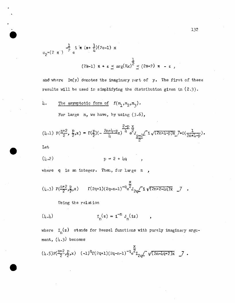
1

(2s-1) ri + e ~ arg(Kx)2 ~ (2§+?) n - e ,

132

and'where Im(y) denotes the imaginary part of y. The first of these

results will be used in simplifying the distribution given in (2.3).

For large n, we have, by using (3.6),

2-p x

(4 .1) F(~, ~,x) = r(~)( - 2n41-J.-px)4e2Jp_~-i J('2n+4·-p)x_7+o( 2n:4-p).

2'"Let

p = 2 + 4q

TftThere q is an integer. Then, for lar ge n ,

( ) n+2 p )).+.3 F(2'~'x

x

r(2Q+l)(2Q-n-l)-qe2J 2c1"i v'('2n+2-4q)x _7 •

Using the relation

I (z) = i-n J (iz)n n

,

where I (z) stands for Bessel functions with purely imaginary argu­n

ment, (4.3) becomes

x

(4.5)F(n;2,~,x) (-1)Qr(2Q+l)(2Q-n-l)-Qe212qL-V(2n-4Q+2)X _7 .

133

Using this, we can write the joint density function of ~;m2 and m3

as

2_ ~ (ki+k~) p~? n-~-l

(4.6)f(mlm2m3)~d~dm3=ce IMI I I-MI

eXI p _2 l'"J( 2n~4-p )x '-r.&'].dm~dm.3 •-r

for all p satisfying (4.2); where

4A. The difficulties in proceeding further.

Various methods have been tried to proceed beyond this point,

but none seems to work well. The main difficulty, even at this stage,

is, that the coefficients in the expansion of the Bessel function in-

volved are increasing. As a consequence of this one would not be

justified in omitting terms in the expansion of I 2 ~/2n+4~px 7p- -2

beyond the first few, and discuss'the distribution of nm3

• The

difficulty would probably be removed if we consider small values ~f

n, and try to integrate over the 16ns-shaped region of Chapter IV to

find the distribution of m3

, but the objection to that would be that

m3

or TIm3

is not a suitable statis0ic for small values of n. This

discussion, therefore, had to be left at this point.

5. The distribution of U for large n ~ p~l, an independent

.§.pproach.

134

The statistic U reduces to z(y_x)/a2 for large n, since

2s is then found from a large sample, and can therefore be replaced

by c/ to which it approximates. This does not imply that the

sample means can also be replaced by their population values since

for n to be large it is enough that one of the sample sizes is large.

Moreover, none of the means has as many degrees of freedom as the var-

iance.

The distribution of z(y-i)/a2 can be found under both the

hypotheses

(1)

as follows.

z e)[l which is

z e)(2 which is

Let Z 6 lTl • The statistic U can be taken as the product of

two normal variates z which is * y-xz =2 which isa

(~N 2a

We can, instead of z and z*, consider the variables u and

v, where u is N(m,a2) and12

v is N(O,a ), where

12a = \I-lJ.and m => lJ. .. T or

a

\I-~ \T\I ..~ , according as z e )'1 or

a

z eJT2 •

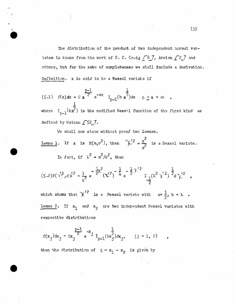
135

The distribution of the product of two independent normal var-

iates is known from the work of C. C. Craig /-8 7, Aroian L-2 7 cmd- - -others, but for the sake of completeness ",re shall include a derivation.

Definition. x is said to be a Bessel variate if

as

,1"2

I l(b x )dxp-

p-l

f(x)dx = C x2 e-ax

1

I (b~2) is the modified Bess~1 function of the first kindp-l

(5.1 )

where

We shall now state without proof two lemmas.

2 IV. r2 x 2Lemma 1. If x is N(m,a), then ~' =~ is a Bessel variate.

a

222In fact, if A = m /a , then

,

'V 12which shows that " is a Bessel variate with 1a= -, b '" A

2

Lemma 2. If xl and x2 are two independent Bessel variates with

respective distributions

p-l 1~ -x 2

f(x Jdx. '" ex. e j I l(bx. )dx.,J J J P- J J

(j -= 1, 2) ,

then the distribution of ~ = xl - x2

is given by

_-b,2 2p-l2 ~ ~

f(~)d~== ~---(-);n 2

~o (E)2r ~2 ( )£J ----"'- K 1 ~ d~,

r==O 2 rtr(p+r) p+r--2

136

where Km(~) is the modified Bessel function of the second kind as

defined by Watson, or in vJhittaker and Watson i-,4, p. 373 _7.

The distribution of U == uv where u is

Let u V'!'"l::t-';"-'I 0- 0-'

and y u v== -

<'.J 0-

where 1") is N(~, 12) and t is N(~, /2).0- 0-

Thus by lemma 1, both

1")2 and ~ 2 are Bessel varia:. ss with2 1

a = 1, b = m2 and p = 2 as0-

parameters; and by lemma 2, theref~re) th8 distribution of the product

is given by

00

Zr=O (1) 2rrtr r+ 2 2

and by noticing that

lATe can rel-rrite this as,

1 m2:'2 .~

0-f(n )dU == _8__

n

00 2r Ifz (E1) ...!.- K (U)dU

r=O () ( 2r ) 1 r

v-IJ.Replacing m by IJ. - ~(j'

I

v-~"""and by v - ---, we get the distri­2

0-

137

butions under the two hypotheses.

6. The asymptotic mean and variance of the statistic U =

z Zi j

ij (- -)s z. y. - x. by the differential method.~ J J ~------....:..;.....;;.---

1r.fe shall, in this section, find the mean and variance of U,

approximately for large samples, by a method which was formerly quite

pooular and still is sometimes used. The object of the section is

mainly to exemplify this method, which can somctliues be aoplied in

getting moments of an unknown distribution. Some of the sets of condi-

tions under which the method is apnlicable are discussed by Cramer

1.-9 _7 in Chapter 27, but we shal], like statisticians in the oast,

apoly it ~Jithout stopping to verify the validity of the application.

Because of the heavy algebra involved it will be enough if we con-

fine ourselves to the discussi.on of the first two moments.

I'

(6.1)

Let

U ij - -)= l: l: s z.(y.- x.i j ~ J J

be written as

(6.2)

where

b.z.l l

,

(6.3)

IrITe define

•

Then

ds ..lJ

138

Follmvinp this (:kiini t ~ on, We' let

(6.6)

where

,

T,Te note that

(6.8)

10 find E( dsij

) :

i'Let s J be, expanded in Taylor's series. irve have

Therefore

... .

Since E(ctskl

) = 0, this reduces to

, . 2 ij(6.10) E(ds iJ )= 12E/-E l. ~ 6 d ° dsk1dS t + ••• 7

.-klrt'o0kl0(jrt r

To evalu3te this, we havE to find

()2(jij

o °kl'() artand E(dskldsrt )

The let ter of these is known from Hot-dling L-23_7 as

(6.12)

139

0' 0' +0' 0'E(ds ds ) = kr It kt ~r

kl rt. n

To find the second ~rder derivatives involved we proceed ,as

follows:

Consider the identities

.. .(I1:O'J.JO' = 5Ji ik k

o

if k = j

if k f j

•

Differentiating (6.13) partially with respect to 0' AaI'" we have

(6.14)

where

(6.15)

Using

if i = k = a = ~

otherwise

(6.16) kmZ. O"kk J.

= orr:J.

in (6.14) and simplifying, we get

(6.17) ,

which provides a formula for the first derivatives.

If the covariance matrix Z is the identity matrix, as can be

supposed for the statistic U, which is known to be invariant under non-

singular linear transformations, then the crls can be replaced by

Kronecker deltas with the same suffices. Thus (6.17) simplifies to

..e

which states that

,

(6.19)

(6.20 )

(J ••~~

= - 1

:= - 1

,

and that the derivative wUh respect to any other element is zero.

To obtain we differentiate partially with re-

spect to crye the equation~

(6.21)

This giv8S~

Using (6.21) in (6.22) and replacing tho cr's by 6's as before, we

obtain

..

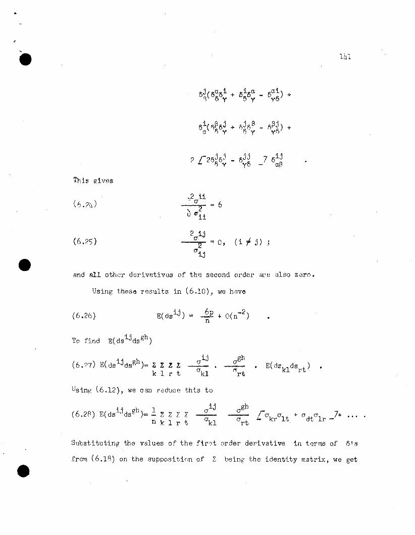
141

This gives

,2 i1... (]

". 2o ('Ji1

-= 6

(6.25)2 ij(]

--"2:- == 0,(1ij

(i =f j)

and all other derivatives of the second order are G180 zero.

Using thes~ results in (6.10), we have

(6.26) 6p (-2)- ... 0 nn

(6.?7) E(dsijdsgh ); ~ k Z !k 1 r t

gh(J

• I'Trt

Using (6.12), we can reduce this to

(6.2~) E(dsijdsgh )= ~ ~ L L 1n k 1 r t

ij(J-(Jkl

~3ubstituting the values of the first order derivative in t8rms of ots

.from (6.18) on the supposition of Z bei.n€ the identity matrix, we get

..e 142

In terms of a's we can use the notation

say

(6.30)

These results will now be used in finding E(U) and Var (U) •

(6,31)· To find E(U)

Since are allindependently distributed, the

expectation of the product is equal to the product of the expectations.

if z eTC.1.

E(Y. - x.) ::: v. - IJ.. =: d. sayJ J J J J

Thus

=.{~+~.2.E

n

if i = j

(6.35) E(U) -' 6- 2; L. IJ.. ( v. - IJ..) / 6~ -} -E 7 .i j 1. J J - ..l. n-

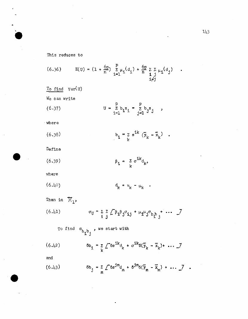
..e

This reduces to

(6.36)6 p 6

E( u) = (1 + -E) ~ I-L. (d.) + .J? ~ ~ I-L' (d.)n i=l ~ ~ n i j ~ J

ir'j

To find var( U)--We can write

(6.37)

. where

p pU = ~ b.z. = ~ b.z.

i=l ~ ~ j=l J J,

Define

(6.39)

where

~. =>J.

(6.hO)

Then in )(1'

(6.1.j.1)

To find

and

O"u :: ~ ~ /-~.~.O" •. + I-L..:I-L 'O"b b + ••• _7. . - J. J J.J J. J . .]. J ]. J

• 144

From these t111]O equations:

Since

from (6.3°) and

(6.46)

can be written as

ButJ'mZo 0

m kIn

therefore we obtain

{

I if j=k

~ ° otherwtse.,

(6.48) . ~ ~ ~jkIn d d + rTij (_1 1)

O'b •b ,'-'/ i.J i.J 1; v N +-1 J k m n ~ m 1 N2

Using (6.48) in (6041), we get

(6 49) 2 '" '" fA A ( '" 'I' 0 ijkIn d d + O'ij (2: + 1: )J].. °u ,-./ i.J {..J I'" 'I-' jOi' + !-L.!-L. i.J i.J k Ni j 1 J ~ J k m n m 1 N2

Replacing ~i and ~j by their values from (6.39), we reduce this to

2 . 'k . °i 'kIn i' 1 l'(6.50) O'u-v Z Z l, Z /-0

1 oJmO",. +~ !-L,!-L, 7dkd + Z LoO J(._ +~.dh.t:'!-L' 0

::!. j k m - 1J n 1: J - m i j N1 N2 .' 1 J

If we supoose that Z = I, then (6.50) reduces to

•(6.51)

where

2 1\1 A 2 1 (1 1) 2aU u + - Z Z Z Z IJ.-IIJ.. dkd 5" kIn + P -N + -N f.Li·

n i j k m ~ J m lJ '1 2

!:J. = Z Z akm dkdk m m

•

7. Correction term for the variance of the linear discriminant

function.

In this section we shall find the variance of the statistic

(7.1) ~f- ij (- -)U =Z:Za y.-x.i j zi J J

,

which is the same as U with ijs replaced by ija because of the

supposition that n is large. If Nl and N2

are both large then

- -Yj - xj

can be replaced by the corresponding difference in the popu-~~

lations, namely v j - IJ.j' giving for U a linear function of normal

variates. As an improvement we shall find the variance of U* by

taking into account the sampling flucutations due to the difference ~f

sample means.

We have

E(y.) := V.J. 1

Let

E(x·-!J.i)(X'-IJ..) = a i . = E(y.-vi)(y.-v.)1 J J J 1 J J

== E(z.-IJ..)(Z.-IJ..)1 1 J J

d. == \J. - "i1 J. J-

•

146

and/

The correction term for the variance of U* *is the variance of U

on the assumption that z = (zl' z2' •.. , zp) is fixed.

U:1f- "" ":' ')' (Jij(-y. -)£, u - x, z.i j J J ~

can be written as

where

so that

w =r

Y -x. r r ,

(7.8)

Hence

(7.10)

and thus

* /~ 1 ~ ~ ~ij5U = - + - (.J '-- v ow. Z i 'V N1 N2 i j J

f2(J

5U*

•which will give the correction term. Since

147

buti' .

Z cr. (J J = 5Ji J.r r

,

and

z Z crij 1'1. d. := tJ 2 say.i j J. J

(7 .12) gives

i' 2E Z l cr J z.z. = p + 6i j ~ J

Adding this to the variance of the linear discriminant function

we have, for the corrected variance,

(7.16) 2 (1 1 1) A2 (1 + 2: )

(J ::: + - + - L.\ + P -Nu* Nl N2 1 N2

This formula shows that the variance 62 based on the assumption

and N2 are larrge tt is an underestimat e of the correct variance of

the discriminant function, but that the difference approaches zero

as rapidly as N1 and N2 approach infinity.

liN1

• CHAFTER VII

SOME RELI\TED UNSOLVED PROBIEMS

In this chapter we shall describe very briefly some unsolved

problems related to the problem of classification.

1. On classification statistics of Wald and Anderson.

(a) The preceeding discussion deals mainly with the distri-

bution of the approximate statistic v = nm) ,that is the statis­

tic whose distribution approximates the distribution of V where

nm..,V =: ----~.:>-2

(l-~)(I-m2)-m3

for large n. 1rJe have discussed mainly the

null case, and much work needs to be done in getting its distribu-

tion in the non-null Gase for the two statistics,

(1) Discussed by 1tfDld L-50 _7(2) Discussed by Sitgreaves L-45 _7 •

(b) The exact treatment of the sampling distribution of V,

both in the central and the non-central cases is still wantinge

2. The quadratic discriminators.

Let ~ and v denote the mean vectors of two p-variate normal

populations, and Zl and Z2 the two covariance matrices. There are

three s:ttuations that may arise in discussing the problem of classi-

fication, namely

•and

( a)

(c)

,

149

If we suppose all the population parameters to be known, then

in these three situations we get the following three statistics,

ij ( )U == Z Z a z. v. - ~.a i j 1. J J

7

where in U, r crij 7 == j-cr .. 7-1 , L-cr.. 7 being the conunon co-a I.. - - l.J- l.J -

d ij ij* Uvariance matrix of the two populations, an ~ , cr in band

U refer to the two covariance matrices in the two populations.c

Thus the distribution problem underlying (2.1) (b) and (c) are those

of a general indefinite quadratic form with zero expectations of the

normal variates in (b) but not in (c). The importance of this prob-

lem has been stressed by Hotelling ;-22 7. ThiS, of course, is under- -the assumption that the population parameters are known which amounts

to saying that N1

-> 00 and N2-> 00, and would be a first step

in discussing the distributions of the statistics

Wb :: Z Z (z. - x. )( z. - i.) ;-sij - sij* 7•• 1. 1. J J- -1. J

and

•r - )( - ) ij - )( - ) ij* 7W = EEL zi - x. z. - x. s - (z. - y. z. - y. s ,

c ij ~ J J ~ ~ J J -

which ~re obtained from Ub and U by replacing the pnpulationc

values in and U by their estimates from the samples.c

3. PossibHity of a different approach.

(a) It may be desirable to discuss the distribution of U =

ij (- -) b . ddt th d ~Tery often ,_'t 4S as zi Yj - x j Y some ~n epen en ms o. ~ ~

good start to examine in what form the non-centrality parameters would

enter into the distribution. The answer to this sometimes ~rovides a

key to the solution of the distribution problem. Furthermore some

questions related to the behavior of the test can be answered even

without finding the actual distribution in the non-null case.

(b) It might be worth while to try some altogether different

approach. It is pass iblG that we run into some si. mpler distribution

problems. Papers of Rao L-32 _7 and Roy L-;5_7 should be useful in

this connection.

4. Efficiency.

(a) The idea of efficiency in problems on classification needs

to be developed systsmatically. Kossack L-26__7 took I-P as the index

of efficiency where P is the common prohability of the; two types of

misclassification ove~ v3ri3tions of the parameters involved. He j

however, considered only the univariate case. Pitman L-37_7 defined

it as the ratio of two sample sizes.

·...,

• 151

These and other idEAS CAn be 8xJmined in this connection.

(b) If therc, Are marc: st"ltisttcs thAn one for the SAm8 situ?-

tion, th,,"1 some m(~3SUrC of rc19tiv·, efficiency is needed.

(c) The discriminant function of R.n. Fisher or the statis­

tic ~ Z a ij z.(v. - ~.) ~re b3sed on the ass~~ption that ~l = L2 •i j ~ J J

One important problem that calls for investigJtion is to eXJmine how

good is the lineBr discrimin1nt function when 3ctually ~l f Z2 •

5. The': greater mean vector.

that even in the univariate case of SJrting numerous objects 'mown

to belong to one or the other of two norm~l populations with the same

known variance, the obvious rule of classifying an object to the popu-

l:3tion WhOS,3 meAn is closer to the me·'Jsure of the object, may not bG

the best rulo. Their ob,jc::ctions'1pply to the corresponding multi-

v:)ri9to situ~ltions and should be considered in problems of cl!Jssifi-

cation in multiv3ri:ote 3nAlysis.

• 152

BIBLIOGRAPHY

F 1 7 Anderson, T.W.,"Classification b;r Multivariate Analysis lf,

- - Psychometrika, Vol.XVI(195l), pp. 31-50.

/- 2 7- -

;- 6 7- -

14rion, L. A., liThe Probability Function of the Product oftwo Normally Distributed Variables II, "~nnals of Mathe­matical Statistics, Vol. XVIII(1947), pp. 26S-271.

Bahadur R.R. and Robbins H. E., '~e Problem of the GreaterMean ll, l\nnals of Mathematical St~ltistics, Vol. XXI (1950),pp. 469-487.

Batemen, Harry, Higher Transcendental Functions. Vol. I andII, McGr C1iI Hill Book Compm y, Inc.,. 1953.

Bose, R. C., liOn the Exact Distribution and Moment Coeffi­cients of the D2-statistics ll , Sankhya, Vol. II (1935­1936), pp. 143-154.

Chernoff, Herman, "Large Sample Theory!!, Annals of MCjthe­matical Statistics, Vol. XXVII (1956), pD. 1-23.

Cochran, t.v. G. and Bliss, C. I., "Discriminant Function withCovariance", .';mals of Mathematical Statistics, Vol.XIX (1948), pp. 151-176.

Craig, c. C. "On the Frequency Function of xy", Annals ofMJthematical Statistics, Vol. Vrr(1936), pp.-l-IS.

Cramer, Harold, Mathematical Methods of Statistics. Prince­ton University Press, 1951.

Fisher, R. "" ''The Us e of Multi pIe He asurements in TaxonomicProblems", Annals of Eu~enics, Vol. VII(1936), pD. 179­188.

L-ll_7 F~she:c, F.~ ,~.,.. HTne St[lti6tic~1 Utilization of ~/Qltiple Measure­ments fJ , Annals of Eup.enics, Vol. VIII(1938), pp. 376-386.

Fix, Evelyn, and Hodges, J. L., "Discriminatory Analysis: Non­Parametric Discrimination: Consistency Problemsll, Schoolof ~viation Medicine. Project number 21-49-004 (1951).

Ford, W. B., Studies in Divergent Series and Summability. TheMacmillan Co., New York, 1916.

Goursat, Edourad, (Hedrick,E.R.,translator), Ii Course inM·JthemBtical Analysis. Vol. I, Ginn and Company, New York,1904.

.J

..

153

Grad, Arthur, and Solomon, Herbert, "Distribution of QuadraticForms and Some "~pplic ations II, Annals of Malthematic a1Statistics, Vol. XXVI(1955), pp. ~64-477.

Gurland. John, "Distribution of Quadratic Forms and Ratios ofQuadratic Forms II, :mnals of Mathematical Statistic.§, Vol.XXII (1953), pp. 416-427.

Gurland; John, "Distribution of Definite and Indefinite Quad­ratic Forms", .Annals of Mathemct.ical Statistics, VoLXXVI(1955), pp. 122-128.

Harter, H. L. nOn the Distribution of Waldls ClassificationStotistic II, Annals of l"Iathemat ical Stat istics, Vol. XXII(1951), pp. 58-67.

HotGlling, Harold s llNew Light on the Correlation Coefficientand its Transforms", Journal of the Royal StatisticalSociety, Series B, Vol. XV, No.2 (1953), pp. 193-232.

L-20_7 Hotslling, Harold, Notes on ~pproximation Techni~ues. (unpub­lished), 1955.

Hotelling, Harold, "Some New Hethods for the Distribution ofQuadratic Forms II ,;~bstract, Annals of ~1athematical Statis­~, Vol. XIX (1948), p. 119.

Hotelling, Harold, IlWlul tivIJriate"ncil.ysis ", Statistics andMathematics in l1iolop-y, Iowa State College Press, (1954),Dp. 67-80.

Hotelling, Harold, "Relation SetTrJeen Two Sets of V9riates !',Biometrika, Vol. XXVIII (1936), pp. 321-377.

Hotelling, H::irold, liThe Generalization of Student I s Ratio ll ,

,mnals of Mathematical Stqtistics, Vol.II(1931), pp. 360­378.

Hotelling, Harold, IlA Generalized T-test and Measure of Multi­variate Dispersion II, Second Berkeley Symposium on iVlath­ematical Statistics and Probability, University of Cali­fornia Press, 1951, pp. 23-41.

Isaacson, S. L., "P:Klblems in Classifying Populations ll , Statis­tics and M3thematics in Biology. Iowa State College Press(1954), pp. 107-119.

...

F27 7- -

;-32 7- -

154

Kendall, M. G., Notes on Mill tivariate t:nalyses, Institute ofStatistics, mimeograph series No. 95, (1954).

Kolmogoroff, A. N., Found3tions of the Theory of Probability.Chelsea Publishing Company, New York, (1950).

Kossack, C. F., flS ome Techniques for Simple Classification rr ,Proceedings of the Berkeley Symposium on MathematicalStatistics and probability, (1945-46), pp. 345-352.

Laha, R. G., IDn Some Properties of the Bessel Function Dis­tribution", Bulletin of the Calcutta Mathematical Society.Vol. XVVI, No.1, (1954), pp. 59-72.

MacRobert, T. M., Functions of a Complex Variable. SecondEdition, Macmillan and Company, Limited, London, 1933.

Mann, H. B. [md Wald, Abrahan, nOn Stochastic Limit and OrderRelationship", flnnals of JVIathematical Statistics, Vol. XIV,(1943), pp. 265-275.

McCarthy, M.D., ("'On the Application of z-test to RandomizedBlocks ll

j Annuals of Mathematical Statistics, Vol. X(1939),pp. 337-359.

Mises, R. V" lIOn the CIa ssific.stion of Observed Data intoDistinct Groups", linnuals of J.VIathematical Statistics, Vol.16, (1945), pp. 68-73. .

Neyman, Jerzy, and Pe ar'son, E.S" IfContributions to the Theoryof Testing Statistical Hypotheses ll , Statistical ResearchMemoirs, Vol. 1(1936), pp. 1-161.

Ogawa, Junjiro, "Remark on Wald's Paper On a Statistical Prob­lem ~rising in the Classification of an IndividUal into Oneof Two Groups", Institute of Statistics, Mimeograph SeriesNo.

Pachares, James, "Note on the Distribution of a DefiniteQuadratic FormB

, _Annals of Mathematical Statistics, Vol.XXVI(1955), pp. 128-ljl.

Pearson E.S. and H3rtley, H. 0., Biometrika Tables for Statis­ticians, Vol. r, cambridge, at University Press, 195&.

.' 155

PeErson, K9rl, Tables o£ Incomplete Beta Functions, CambridgeUniversity Press, 1934.

Pitman, E.J.G., Lecture Notes on Non-Parametric StatisticalInference. (unpublished).

£38_7 Rao, C. R., liThe Utilization of Multiple Measurements inProblems of Biological Classification ll , Journal of theRoyal Statistical Society, Series B, Vol. X (1948), pp.159-193.

Rao, C. R., Advanced Statistical Methods in Biometric Research.John Wiley and Sons (1952), New York.

Rao, C. R., IlA General Theory of Discrb':.ination lk1hen the In­formation about Alternative Popu.lations is based onS3mples ll , Annals of Mathematical Statistics, Vol. XXV(1954),pp. 651-670.

Robbins, H. E. and Pitman,E. J. G., r,r'"\pplication of the Methodof JVrl.xtures to Quadratic Forms in Normal Variates II, l.nnaJsof Mathematical Statistics, Vol. XX (1949), pp. 552-560.

Robbins, H. E., IlAsymptotically Subminim:ax Solutions of Com­pound Statistical Decision Problems~l, Proceedings of theSecond Berkeley Symposium in MClthematical Stat istics andProbability, University of California Fress, Berkeley,pp. 131-148"

L-43_7 Roy, S. N., '~n a Heuristic Method of Test Construction, andits Use in l'1ultivariate l\nalysisr,~, Annals of lVIathematicalStatistics, VoL XXIV, 1953, pp. 2~O-238. -

Roy $ S. No, A Report on Some Aspects of Multivari %e Anci.l. ysj_s,North Cl1lrolina Institute of Statistics, Mimeograph Series,No. 121, 1954.

Sitgreaves, Rosedith, liOn the Distribution of Two RandomMatrices used in Classification Procedures fl , Annals ofMathematical Statistics, Vol. XXIII(1952), pp. 263-270.

Smith, C.A.B., "Some Examples of Discrimination ll , A,nnalsofEugenics, Vol. 13(1947), pp. 272-2820

Stekloff, W., lIQuelques l\pplications Nouvelles de la Theoriede Fermeture au Problemede Representction Approchee deMoment.s l!, Memoire de l'"icademie Imperiale des Sciencesde st. Petersbourg. VoL XXXII, NO: 4, (1914), pp.

t.

r!

-e

1506

£)~8 7 S'Zeg0l'Gabor, Orthogonal Polynomials. American !1athematical- Society Colloquium Publication, Vol. XXIII, 1939.

/-49 7 Uspensky, J. V., Introduction to Mathematical Probability.- - McGraw Hill Book Compffiy, Inc., 1937~

i-50 7Wald, Abraham, r~n a Ststistical Problem Arising in the Classi-- fication of an Individual into One of Two Groups rr, Annals

of Mathematical Statistics, Vol. XV, 1944, pp. l45-Ib2:--

L-5l_/1ATald, Abrahan, Selected Papers in Statistics and Probability.McGraw-Hill Book Company, Inc., New York, 1955.

L-52_7 Watson, G. N., Theory of Bessel Functions. Second Edition,Cambridge University Press, 1945.

L-53 7Welch, B. L., tlNote on Discriminant Functions"i, Biometrika, Vol.- XXXI (1939), pp. 218-220.

/-54 7 Whittaker, E. T. and Watson, G. N., A Course of Modern An~Y8is.- - Fourth Edition, Cambridge University Press, 1952.

i-55 7Wilks, S. S., nOn Some Generalizations of the Analysis of Var-- iance", Biometrika, Vol. XXIV. (1932), pp. 471-494.