onboard impedance diagnostics method of li- ion traction

Onboard impedance diagnostics method of Li-

ion traction batteries using pseudo-random

binary sequence

Charalampos Savvidis

Zeyang Geng

Master Thesis

Department of Electrical Engineering

LiTH-ISY-EX--15/4872--SE

iii

Onboard impedance diagnostics method of Li-

ion traction batteries using pseudo-random

binary sequence

Master Thesis in method evaluation and feasibility study of concept

Department of Electrical Engineering

Division of Vehicular Systems

Linköping University


Zeyang Geng

LiTH-ISY-EX--15/4872--SE

Supervisors: Ylva Olofsson, Jens Groot, Martin West

AB Volvo, GTT, Advanced Technology & Research

Sergii Voronov

ISY, Linköping University

Examiner: Mattias Krysander

ISY, Linköping University

Linköping, 10 June, 2015

v

Presentation date

2015-06-10

Publication date

2015-0x-xx

Institution and Department

Department of Electrical Engineering, Integrated Circuits and Systems

URL for electronic version

http://www.ep.liu.se/

Publication title

Onboard impedance diagnostics method of Li-ion traction batteries using pseudo-random binary

sequence

Authors

Charalampos Savvidis, Zeyang Geng

Abstract

Environmental and economic reasons have lead automotive companies towards the direction of EVs and HEVs. Stricter emission legislations along with the consumer needs for more cost-efficient and environmental friendly vehicles have increased immensely the amount of hybrid and electric vehicles available in the market. It is essential though for Li-ion batteries, the main propulsion force of EVs and HEVs, to be able to read the battery characteristics in a high accuracy manner, predict life expectancy and behaviour and act accordingly. The following thesis constitutes a concept study of a battery diagnostics method. The method is based on the notion of a pseudo-random binary signal used as the current input and from its voltage response, the impedance is used for the estimation of parameters such as the state of charge and more. The feasibility of the PRBS method at a battery cell has been examined through various tests, both in an experimental manner at the lab but also in a simulation manner. The method is compared for validation against the electrochemical impedance spectroscopy method which is being used as a reference. For both the experimental and the simulation examinations, the PRBS method has been validated and proven to work. No matter the change in the parameters of the system, the method behaves in a similar manner as in the reference EIS method. The level of detail in the research and the performed experiments is what makes the significance of the results of high importance. The method in all ways has been proven to work in the concept study and based on the findings, if implemented on an EV’s or HEV’s electric drive line and the same functionality is observed, be used as a diagnostics method of the battery of the vehicle.

Index terms

Li-ion batteries, hybrid vehicles, EIS, PRBS, state of charge, state of health, battery diagnostics


vii

Linköping University Electronic Press

Copyright

The publishers will keep this document online on the Internet – or its possible replacement –

from the date of publication barring exceptional circumstances.

The online availability of the document implies permanent permission for anyone to read, to

download, or to print out single copies for his/hers own use and to use it unchanged for non-

commercial research and educational purpose. Subsequent transfers of copyright cannot

revoke this permission. All other uses of the document are conditional upon the consent of the

copyright owner. The publisher has taken technical and administrative measures to assure

authenticity, security and accessibility.

According to intellectual property law the author has the right to be mentioned when his/her

work is accessed as described above and to be protected against infringement.

For additional information about the Linköping University Electronic Press and its procedures

for publication and for assurance of document integrity, please refer to its www home page:


© Charalampos Savvidis, Zeyang Geng


ix

Abstract

Environmental and economic reasons have lead automotive companies towards the direction

of EVs and HEVs. Stricter emission legislations along with the consumer needs for more cost-

efficient and environmental friendly vehicles have increased immensely the amount of hybrid

and electric vehicles available in the market. It is essential though for Li-ion batteries, the

main propulsion force of EVs and HEVs, to be able to read the battery characteristics in a

high accuracy manner, predict life expectancy and behaviour and act accordingly.

The following thesis constitutes a concept study of a battery diagnostics method. The method

is based on the notion of a pseudo-random binary signal used as the current input and from its

voltage response, the impedance is used for the estimation of parameters such as the state of

charge and more.

The feasibility of the PRBS method at a battery cell has been examined through various tests,

both in an experimental manner at the lab but also in a simulation manner. The method is

compared for validation against the electrochemical impedance spectroscopy method which is

being used as a reference. For both the experimental and the simulation examinations, the

PRBS method has been validated and proven to work. No matter the change in the parameters

of the system, the method behaves in a similar manner as in the reference EIS method.

The level of detail in the research and the performed experiments is what makes the

significance of the results of high importance. The method in all ways has been proven to

work in the concept study and based on the findings, if implemented on an EV’s or HEV’s

electric drive line and the same functionality is observed, be used as a diagnostics method of

the battery of the vehicle.

Index terms: Li-ion batteries, hybrid vehicles, EIS, PRBS, state of charge, state of health,

battery diagnostics

xi

Acknowledgments

For the completion of the thesis work I would like to thank first and foremost Martin West,

Ylva Olofsson and Jens Groot from AB Volvo, Group Trucks Technology, Advanced

Technology and Research, without their insight and their continuous guidance the completion

of this thesis would be impossible.

Special thanks must be accredited to my partner in the thesis work, Zeyang Geng, for all her

patience and will to help and guide me in the progress of the work.

I would also like to thank Professor Mattias Krysander and Sergii Voronov from Linköping

University for allowing me to perform the thesis for the department of Electrical Engineering,

for all the information they provided me when needed and for their valuable feedback.

Finally, I could not thank enough my family, my friends and especially my girlfriend, Jessica

Kindström, for their endless support and encouragement throughout the duration of the work.

Linköping, June, 2015


xiii

Contents

1. Introduction ....................................................................................................................................... 1

1.1 Problem Background ............................................................................................................... 1

1.2 Previous Work ......................................................................................................................... 2

1.3 Purpose .................................................................................................................................... 4

1.4 Limitation................................................................................................................................. 4

1.5 Outline ..................................................................................................................................... 5

2. Electric drive line and traction battery system ............................................................................... 7

2.1 Electric drive line ..................................................................................................................... 7

2.2 Li-ion battery ........................................................................................................................... 8

2.3 Battery model .......................................................................................................................... 8

2.4 Battery diagnostics on vehicles ............................................................................................. 11

2.4.1 Inputs to diagnostic evaluation ......................................................................................... 12

2.4.2 Outputs from diagnostics evaluation ................................................................................ 12

2.5 Parameters identification on battery .................................................................................... 13

2.5.1 Electrochemical Impedance Spectroscopy (EIS) ................................................................ 13

2.5.2 Pseudo-random binary sequence (PRBS) .......................................................................... 15

2.5.3 Selection of PRBS parameters ........................................................................................... 17

2.5.4 Non-parametric system identification .............................................................................. 18

3. Case setup ......................................................................................................................................... 21

3.1 Experimental setup ............................................................................................................... 21

3.1.1 Assumption ........................................................................................................................ 21

3.1.2 Experimental procedure .................................................................................................... 22

3.1.3 Hardware setup ................................................................................................................. 23

3.1.4 Parameters selection ......................................................................................................... 26

3.2 Simulation setup .................................................................................................................... 32

xiv

4. Implementation in the vehicle ........................................................................................................ 35

4.1 Motor model and control algorithm ..................................................................................... 35

4.1.1 Motor model ..................................................................................................................... 35

4.1.2 Motor controller ................................................................................................................ 36

4.2 Simulation of the PRBS on the driveline................................................................................ 37

4.2.1 Simulation model of the driveline ..................................................................................... 38

4.2.2 Speed operation range ...................................................................................................... 39

4.2.3 Parameters selection of the PRBS in the driveline simulation .......................................... 40

4.3 Results and analysis ............................................................................................................... 42

5. Experiments, simulations and analysis .......................................................................................... 49

5.1 Experimental results .............................................................................................................. 49

5.1.1 Signal processing ............................................................................................................... 49

5.1.2 EIS measurement at different SOC level ........................................................................... 51

5.1.3 EIS measurement at different temperature ...................................................................... 53

5.2 Simulation results .................................................................................................................. 56

5.2.1 EIS implementation ........................................................................................................... 56

5.2.2 PRBS implementation ........................................................................................................ 58

5.2.3 Method validation ............................................................................................................. 59

6. Conclusions ...................................................................................................................................... 73

6.1 Conclusions from present work ............................................................................................ 73

6.2 Future work ........................................................................................................................... 73

6.2.1 Improvements for the PRBS method................................................................................. 74

6.2.2 Additional options for PRBS implementation on the driveline ......................................... 74

Bibliography ........................................................................................................................................ 75

Appendix .............................................................................................................................................. 79

Battery cell specification ................................................................................................................... 79

Table of simulation experiments ....................................................................................................... 80

EIS, PRBS and validation figures ........................................................................................................ 81

xv

List of abbreviations

AC Alternating Current

DC Direct Current

EV Electric Vehicle

HEV Hybrid Electric Vehicle

MCU Motor Control Unit

BMU Battery Monitoring Unit

SOC State of Charge

SOH State of Health

EIS Electrochemical Impedance Spectroscopy

PRBS Pseudo-Random Binary Sequence

SNR Signal-to-Noise Ratio

BOL Beginning of Life

EOL End of Life

CPE Constant Phase Elements

RMS Root Mean Square

RC Resistor-Capacitor

PMSM Permanent Magnet Sychronous Motor

FOC Filed Oriented Control

OCV Open Circuit Voltage

A Ampere, unit of measure of current

V Volt, unit of measure of voltage

Ω Ohm, unit of measure of resistance, impedance

1

1. Introduction

Ever since the re-appearance of the hybrid electric vehicles in the mid-90s and their bloom in

the worldwide market, the usage of Li-ion batteries in the automotive industry has been

preferred as means of energy storage for propulsion. Until then and till today, the most

common application of the Li-ion batteries was in portable computers, but nowadays the

automotive industry turn their attention to them and their advantages. Attractive features

include the high energy density and the relatively low self-discharge.

Engineers though, are facing the challenge to make Li-ion batteries and their applications in

ways that will be able to predict their life expectancy, degradation and plan production and

future actions accordingly due to the unpredictable nature of the ageing mechanism of

batteries and how it affects their health. Especially when the high cost of the automotive

application of Li-ion batteries is taken into account, one can understand the importance of

being able to use a battery pack of the vehicle to its fullest potential, either if one sees it from

the producer's or customer's point of view. Identification of the battery performance, its

operations and limits, and how they are affected should be calculated and monitored with the

highest accuracy possible in order to avoid expenses in an economic and productive way.

1.1 Problem Background

Automotive companies that offer hybrid or electric variants to their customers usually have

their equipment of estimating the battery performance and act based on that. One of the

problems is that not always the correct approaches and methods are implemented in the

battery monitoring units for the implementation of the battery ageing analysis, thus the

accuracy of the measurements will not be of the desired level and factors such as the

functionality and reliability may be severely affected. There are after-market companies also

that seized the opportunity and offered the ever-growing percentage of hybrid vehicle owners

the technology and equipment for service and diagnostics of the battery performance. These

systems can perform multiple tasks such as full battery pack service and balancing, de-

powering to a safe level after a severe collision, recycling, estimating the battery pack state of

health, determining whether it is becoming weak and inefficient. The high cost of owning

these systems though, along with the technical knowledge needed to operate them, may

constitute these diagnostics systems as difficult to comprehend and therefore not user-friendly

enough.

The state of charge (SOC) and the state of health (SOH) are two parameters that are accurate

with respect to the battery impedance, but most importantly easy to comprehend when they

are used to identify and characterize the battery performance. Especially in the case where the

2

customer of the hybrid vehicle uses the diagnostics system and not an expert or a technician,

the interpretation of the measurements is simplified due to the fact that parameters such as the

SOC are used extensively in everyday gadgets and appliances such as laptops, mobile phones

and more. Parameters as these are essential to be renewed and re-evaluated constantly through

their life, because their functionality and behavior depends mostly on it and the readings of

the diagnostics system should correspond to the real properties. Based on these parameter

measurements, appropriate actions can be planned and performed, either from the

manufacturer like replacing the battery pack of the hybrid vehicle or the customer like how to

use the battery performance on an everyday basis.

The effectiveness of a diagnostics system does not rely on the fact that the user and the

manufacturer can see the state of the battery pack, but more on the fact that with this

knowledge of the battery state no precaution time margin is needed anymore from the

manufacturer. All battery packs of hybrid electric vehicles can be evaluated individually and

treated accordingly, no matter how much time and conditions of operation they have been

exposed to.

1.2 Previous Work

Explanations, analyses and meanings of concepts such as the EIS and PRBS methods, battery

impedance, battery diagnostics and more have been studied in literature such as former

Master and Phd student theses [29] [30], scientific articles, journals and books on batteries

and hybrid vehicles for a better comprehension of the subject. Topics, results and conclusions

from the aforementioned literature, especially from previous Thesis works that have been

performed at Volvo GTT, have been used as reference in the progress and completion of this

Master Thesis report.

Previous work also includes algorithms and simulations models that were used in the past and

shall be used as examination and reference tools for the conduct of this thesis work. One of

the most important simulation models from previous work, not only for its current usability

but for functionality examination also, is the Asterics battery model, depicted in Fig. 1.1. The

Asterics model is a complex, yet simple in its use, simulation model of the functionality of a

battery. The current and the temperature are used as inputs in the model and it produces

results for outputs including the state of charge (SOC) and state of health (SOH).

3

Figure 1.1: The Asterics Battery reference simulation model

Several works have been done to investigate the Li-ion battery impedance behavior,

especially during the ageing [30], [29]. It turns out that the parameters of the battery can be

extracted from the electrochemical impedance spectroscopy (EIS), which can be used to

characterize the battery state. Most of the analysis of the EIS are made on cell level using

frequency swept measurement. The measurement and analysis of the battery EIS for

diagnostics purposes on-board the vehicle level are missing. Texas Instruments has been

developing an Impedance Track Based Fuel Gauging [34]. It can estimate the remaining

capacity for a cell based on its impedance, but it can only be used for single cells in medical

equipment application.

The pseudo random binary sequence (PRBS) is a type of signal used in system identification

[23]. The PRBS has been used in different areas, including the measurement of power grid

impedance [33] and parameters identification of Li-ion batteries [31]. In [32], it is shown that

the PRBS can be used to measure the EIS of the battery and it can give a better result

compared to other signals that are also used for system identification. To be able to measure

the battery impedance on-board, the motor can be used as the load to generate the PRBS

signal as shown in [38]. This paper also shows a very good example about how to calibrate

the measurements.

Other than the PRBS, the system noise can also be used for identification. In [36] the system

noise caused by the telecommunication is used to measure the battery impedance and it shows

good results. In terms of the automotive application, the drive cycle itself can be considered as

the system noise. In [39] the current is being used at the start of the combustion engine as the

4

identification signal in a hybrid electric vehicle. They have built an adapted model which can

represent the aging behavior of the battery and the internal resistance can be estimated. But as

said in [40], the ohmic resistance and the charge transfer resistance can hardly be

distinguished in this case. In [37] the extended Kalman filter is used to observe the impedance

of the battery from an urban driving cycle of a hybrid electric vehicle. This method can get

the impedance of the battery based on a series of RC model which can approximately get the

impedance at very low frequency but cannot describe all the battery behaviors.

What is more, to model the battery in order to represent the EIS, several constant phase

elements (CPE), which are nonlinear components, are needed [27] [28]. This increases the

difficulty for system identification.

1.3 Purpose

The purpose of this thesis work is to examine, through experimentation and simulations, the

feasibility and the applicability of an on-board impedance diagnostics method of Li-ion

traction batteries using the pseudo-random binary sequence (PRBS) method.

The scope of this thesis is to cover identification of the necessary equipment needed to

perform the method on the hybrid vehicle, determine of the impedance data can be used in the

improvement of battery monitoring algorithms, and feasibility analysis of the method. Part of

the thesis scope is the design, with the proper software, of simulation tools to reduce, after

validation, the experimental time, effort and cost.

An on-board battery impedance diagnostics system will give the user or the maintenance

technician of the hybrid electric vehicle the ability to examine important battery parameters

such as the state of health (SOH) that are updated continuously during the battery life and act

accordingly.

1.4 Limitation

The aim of the thesis is to focus on the method evaluation of PRBS for battery diagnostics.

The integration of the impedance measurement to the battery monitoring unit algorithm is out

of the scope. The impedance measurement is assumed to be at the equilibrium condition of

the battery whereas the very slow dynamic behavior of the battery is out of the scope of the

thesis. This thesis focuses on method validation, which is not limited in one type of Li-ion

batteries so the selection for the electrode material is out of the scope. The cell tested in this

thesis is selected by Volvo. Further details are to be explained in Section 3.1.

5

1.5 Outline

The theoretical part of the thesis is described in Chapter 2, including the drive line in an

electric vehicle, the Li-ion battery and its model, the EIS and how to use the PRBS to measure

the impedance. The function of the BMU is also introduced. The experiments and simulation

set-up are described in Chapter 3. A proposal of the PRBS implementation on the vehicle is

presented in Chapter 4, as well as an example of an on-line impedance measurement. The

results are discussed in Chapters 5 and 6. Finally the conclusion and future work are found in

Chapter 7.

7

2. Electric drive line and traction battery system

The electric drive line constitutes the system that enables an EV or HEV to use electricity

from the battery as its fuel and produce motion of the vehicle. The inverter is being supplied

with energy from the battery and with proper control from the BMU and the motor control

unit (MCU), it feeds the motor and propulsion is achieved.

2.1 Electric drive line

The layout of the electric drive line implemented in this thesis work for an electrical vehicle,

shown in scheme in Fig. 2.1, consists of the components explained in detail in the section to

follow.

Figure 2.1: Scheme of a base electric driveline in the vehicle

Synchronous electric motors contain multiphase AC windings in the stator of the motor that

create a magnetic field which rotates in time with the current. They can be found in various

sizes, from sub-fractional self-excited to high-horsepower industrial, and for various

applications. The electric machine to be utilized in the case of the thesis work is a

synchronous motor. According to [8] this kind of motor is an AC motor in which, at steady

state, the rotation of the shaft is synchronized with the frequency of the supply current.

An inverter is an electronic device that transforms direct current to alternating current. The

power is supplied by the direct current source [11].

DC-link capacitors are commonly used on the DC side of the inverter to stabilize the DC side

voltage. They contribute substantially to the volume, the weight and to the cost of the power

8

inverters, in particular a significantly sized DC-link capacitor will add unnecessary cost so the

manufacturers will choose the smallest capacitor possible. A sufficient capacitor will allow

the great majority of the current ripple to flow through the capacitor instead of passing

through the battery, thus making the current from the battery to be fairly constant regardless

of the switching [5].

The electric energy storage system (battery) is a device that consists of one or more

electrochemical cells that converts chemical energy that is stored into electrical energy. A

cathode and an anode are contained in each cell and electrolytes allow ions to shift between

the opposite terminals thus creating flowing current. Batteries come in various shapes and

sizes and can be divided based on their repetition of use in primary or secondary. A primary

battery cell has been designed and manufactured in such a way to be used once and then be

discarded after depletion whereas on the other hand, secondary battery cells are the type of

cells that can be used repeatedly because of their recharging ability and function [9] [10]. In

the conduct of the thesis work all battery cells that are going to be used are secondary. Further

details regarding the battery cells that are used, their chemistry and way of work are to follow.

2.2 Li-ion battery

The Li-ion batteries are widely used in hybrid electric vehicles (HEVs) and electric vehicles

(EVs) due to the high power and energy density [29]. There are a variety of types of electrode

materials for Li-ion batteries. For the cell used in this thesis work, the specification of the cell

is shown in the Appendix, section Battery Cell Specification. This cell has a nominal voltage

of 3.75 V and 41 Ah capacity with Mn/NMC cathode and Carbon/Graphite anode.

The battery capacity is usually presented in Ampere-hours (Ah). One way to describe the

charge/discharge current is to use the term C-rate. The current is normalized with the battery

capacity, for example, 1 C-rate (C/1) means that the current will fully charge/discharge the

battery in one hour, 10 C-rate (C/0.1) will fully charge/discharge the battery in 0.1 hour.

The traction battery, which is also called battery pack or energy storage system (ESS), is the

main energy source in the EVs. When investigating the possibility and the requirements to

implement the EIS measurement on the traction battery, the rated voltage is assumed to be

600 V according to the released data in Volvo 7900 Electric Hybrids, a common level for

heavy duty vehicles [43].

2.3 Battery model

The battery model that is implemented and used for the simulations in the line of the thesis

work takes the current and the temperature as inputs and calculates outputs such as the voltage

9

and the SOC, as shown in Fig. 2.2. Data taken from the simulations (simout data in Fig. A.9),

are used in the implemented algorithms for the further examination of the EIS and PRBS

methods.

Figure 2.2: Battery model simulation

The parameters to be used for all the calculations needed in the battery model such as the

battery nominal capacity, the initial hysteresis, scalars, factors and more, are defined from the

start in a Matlab workspace file and loaded for use when called. The most important of those

parameters and the effect of which is more in line with the scope of the thesis are defined and

altered accordingly for each simulation in the beginning of the controlling algorithm of the

implementation. Such parameters are the initial SOC and SOH, the temperature and more.

The state of charge is being calculated by having the initial SOC, as defined by the user, and

then with the use of scaling functions, Simulink blocks and mathematical equations, the final

value of the SOC is being calculated for the experimental simulation.

The voltage is being calculated through two main component implementations, one from the

OCV calculation and one from the resistance of the battery. The OCV calculation is being

done with the use of proper blocks and equations connecting all the essential parameters along

with a more complex function, implemented for the calculation of the hysteresis of the

battery, with hysteresis being the time-based dependence an output has on input it is subjected

to currently and from the past [43].

10

The resistance on the other hand is being implemented by calculating the double layer

capacitance, the charge transfer resistance, the Warburg capacitance, the polarization

resistance and the ohmic resistance. From the above, the charge transfer, polarization and

ohmic voltage drops are calculated and their sum is the total voltage drop. Equally, the total

voltage drop along with the open circuit voltage are the components to be summed for the

calculation of the voltage output of the battery cell. For the voltage of the battery pack, the

number of cells in series or parallel configuration must be taken into consideration and

calculated accordingly.

The battery model, as implemented, offers the option also to the user to operate the model as a

battery cell or a battery pack. The number of cells that will constitute the battery pack along

with the configuration on which they are going to be placed can be defined and changed for

each simulation, depending on what is examined. When a parallel configuration is used, the

voltage is the same through all the cells and the current is the sum of the currents of each

individual cell, as shown in Fig. 2.3.

Figure 2.3: Parallel connection of four battery cells [42]

In contrary, as it can be seen in Fig. 2.4 in series configuration the current is the one that is the

same throughout the circuit and the voltage is calculated as the sum of all voltages from each

individual cell [42].

Figure 2.4: Serial connection of four cells [42]

11

The configuration depends on the application the battery pack will be used, it is common also

to meet combinations of these configurations in a single circuit system, so there is the

possibility to perform the same in the battery model.

What it can be said, and it is explained by the fact that in a serial configuration the voltage is

constantly added up and subsequently increased, that the layout to be preferred is based on the

needs and expectations one expects from the battery pack. If high voltage is the demand then

a serial configuration must be preferred whereas if high current is to be created then the

recommended configuration is the parallel.

2.4 Battery diagnostics on vehicles

In order to monitor and control the battery operation a battery monitoring unit (BMU) is used.

By operating the battery cell or pack at certain conditions and with the aid of the BMU, the

required states that are to be calculated can be found. The BMU generally takes parameters

such as the battery current, voltage and the operating temperature into account and gives

results regarding the impedance, the SOC and the SOH of the battery.

A battery management system is an electronic system that can manage a battery cell or pack

and perform operations such as protecting the battery from operating outside its safe

operational area, monitor its states, calculate and report secondary data etc. [1]. In particular

the monitoring unit detects the battery voltage, current and temperature as well as other

parameters and produces the required data, as depicted in Fig.2.5.

Figure 2.5: Battery monitoring unit scheme

For Li-ion batteries it is necessary to measure the voltage of each cell, then these analog

voltage data are converted to a digital form and if it is detected that a cell is operating at a

higher voltage it makes it discharge, a procedure known as balancing of the cell [2].

12

2.4.1 Inputs to diagnostic evaluation

Electric current is the flow of electric charge and it occurs when there is a potential difference.

For electric current to flow a complete circuit is required, meaning that the flowing charge has

to have the ability to get back to its starting point. Charge is often carried by moving electrons

in a wire or by ions in an electrolyte [4].

Voltage is the electric energy charge difference of the electric potential energy that is

transported between two points. It is equal to the work that is done per charge against an

electric field to move the charge between two points. Voltage can represent a source of energy

or lost, used or stored energy [14] [15].

According to [3] if a device, the battery in this particular case, is exposed to operation outside

the limits of its temperature range, it will age faster and the risk of failure will be increased.

For Li-on batteries the charging temperature limits are different than the operational, this

means that even though it will function the battery charging will not be as effective in all of

the range. In particular, cooler temperatures of 5 to 45° allow for an optimized fast-charging

whereas low temperature charging (0 to 5°) is possible but the charge current should be

reduced, high temperature charging (above 45°) is not recommended due to the fact that it

degrades the battery performance [18].

2.4.2 Outputs from diagnostics evaluation

Electrical impedance is the opposition that a circuit presents to a current when voltage is

applied [7]. It can be quantified as the complex ratio of the voltage to the current in an AC

circuit and it is the extension of the resistance concept in AC circuits. When the impedance is

caused by the inductance and the capacitance it forms its imaginary part whereas the real part

is formed by the resistance [6]. Impedance increases with ageing of the cell.

State of charge (SOC) is the charge that the battery currently has for any operation and it is

measured in percentage of the fully charged capacity [12].

State of health (SOH) is a measurement that shows the amount of “life” that is remaining in

the battery and it is therefore depicted in a percentage of the total original capacity of the

battery [13]. Typically, the battery SOH will be 100% at the time of manufacturing and will

decrease over time and use, Fig. 2.6. Batteries though, with capacity under 80% are

considered depleted and therefore no more useful on automotive application.

13

Figure 2.6: State of health depiction as the capacity fade with time passing

2.5 Parameters identification on battery

In the following chapter, the methods to be implemented and the parameters at which these

methods are to be investigated are presented. Both methods are explained in detail and are to

be implemented in the battery laboratory and the simulation processes.

2.5.1 Electrochemical Impedance Spectroscopy (EIS)

EIS is one of the most common experimental methods for the characterization of

electrochemical systems and one that is used extensively in battery cell research [17]. In this

method, the impedance of a system over a range of frequencies is being measured, energy

storage and dissipation properties are revealed by the frequency response.

Advantages that have made the method of EIS extensively used in a wide variety of scientific

areas include for example measurements that are not being intrusive, impedance parameters

such as the ohmic and charge-transfer resistance can be estimated from an experiment. In

addition, it is a relatively simple method so procedural simulation constitutes a viable and

usable option with high precision in the measurements because they can be averaged over a

long time to improve the signal-to-noise ratio [16].

A way to depict the EIS method and afterwards interpret and utilize its results is through a

Nyquist plot. For a range of frequencies, the real and imaginary parts of the impedance

constitute the axis of the plot. From the Nyquist plot, the values of important parameters such

as the ohmic and charge transfer resistances can be identified, as seen in Fig. 2.7. The ohmic

resistance is the intersection with the real axis of the impedance curve in the Nyquist plot

whereas the charge transfer resistance is the real impedance approximately at the local

14

minima of the impedance curve in the Nyquist plot [30]. Another important parameter to be

taken into account is the double layer effect, which is the formation of two layers of opposite

polarity at the interface between electrode and electrolyte. This phenomenon occurs when an

electronic conductor is brought in contact with a solid or liquid ionic conductor [44].

Figure 2.7: Ohmic and Charge Tranfer resistance in the Nyquist plot

The importance of these parameters lies on the position they have on an electric circuit. As depicted

below in Fig. 2.8, both the ohmic and the charge transfer resistance constitute important parts of the

circuit along with the voltage supply and more.

Figure 2.8: Generic depiction of an open circuit voltage

15

2.5.2 Pseudo-random binary sequence (PRBS)

The PRBS signal is a band-limited white noise, which can be used to identify a linear system

in a limited frequency range. It switches between two states and it can be generated by a

linear feedback shift register (LFSR) [22]. Details about how to design a PRBS signal and

how to implement it in the computers are well explained in [23]. An example of an 8-bits

PRBS signal is given here.

The PRBS is generated by using the commands Unit Delay and XOR Logical Operator in

Simulink, as shown in Fig. 2.9.

Figure 2.9: PRBS Generator

For an n-bit PRBS, the total number of possible states N is

For an 8-bit PRBS, the registers can have 255 different states. A PRBS that can go through all

the states is called maximum length sequence, which is most of the cases when it is designed

for system identification. The PRBS signal will repeat every N states so it is a periodic signal.

As the bit length of the PRBS is increasing, it will take a longer time to go through every

state. The whole testing time will increase exponentially with the number of bits.

Another important factor for a PRBS signal is the clock frequency, which is the shifting

frequency for the registers. The delay time in the delay unit in Fig. 2.9 is set to be

For example, when the clock frequency equals to 10 Hz and the all the initial states in the

register are 1, the 8-bit PRBS is shown in Fig. 2.10.

16

(a) One period of an 8-bit PRBS (b) Part of the 8-bit PRBS

Figure 2.10: An example of an 8-bits PRBS with 10 Hz clock frequency

The advantage of the PRBS is that it is not correlated with itself within one period. The auto-

correlation function of the 8-bit PRBS is shown in Fig. 2.11(a). This PRBS repeats for three

periods and it can be seen that it is only auto correlated once after one period. Thanks to this

pseudo-random characteristic, the PRBS contains signals in a wide frequency range.

(a) Autocorrelation response of an 8-bit PRBS (b) Fast Fourier Transform of an 8-bit PRBS

repeating for three cycles showing usable frequency

Figure 2.11: The autocorrelation response and frequency domain characteristic of the previous PRBS

The number of bits n and the clock frequency determine the usable frequency range of a

PRBS, which can be studied by using the Fourier Transform, as shown in Fig. 2.11(b). The

usable range is defined by the 3-dB bandwidth (it is called the half power bandwidth) [23].

The minimum frequency, which is the first frequency point after the DC, is

17

and the maximum frequency which is when the amplitude of the signal decreases to 3 dB of

its peak value, is

according to [26]. Ideally, a PRBS signal only contains the information at the certain

frequency points. The frequency step is

Therefore, a PRBS contains usable information at

2.5.3 Selection of PRBS parameters

In the battery reactions, different phenomena have different time constants. The double-layer

effect can reflect the SOC of the battery as shown in Fig. 2.12. So the target of the PRBS

measurement is to capture the double-layer effect.

Figure 2.12: EIS at different SOC level from previous test

The time constant of the double-layer effect depends on the material of the battery. For most

of the batteries, the time constant is in the range of milliseconds to some seconds [41]. For the

18

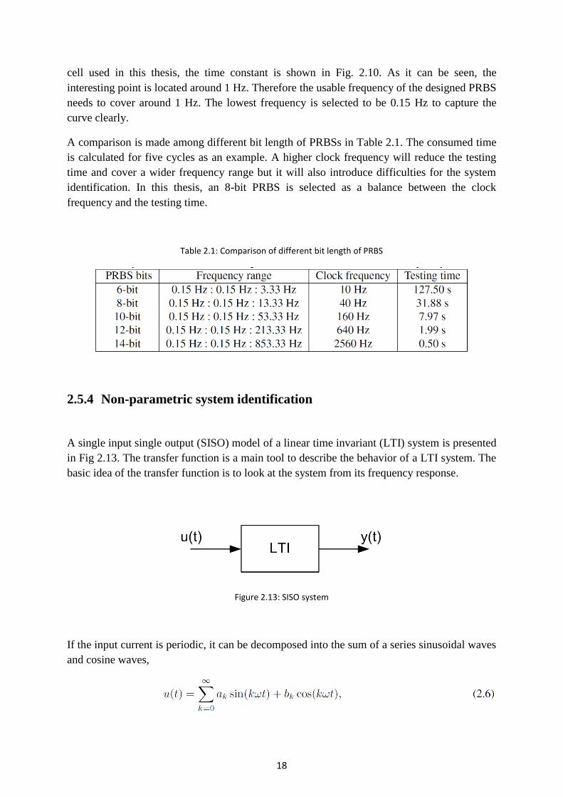
cell used in this thesis, the time constant is shown in Fig. 2.10. As it can be seen, the

interesting point is located around 1 Hz. Therefore the usable frequency of the designed PRBS

needs to cover around 1 Hz. The lowest frequency is selected to be 0.15 Hz to capture the

curve clearly.

A comparison is made among different bit length of PRBSs in Table 2.1. The consumed time

is calculated for five cycles as an example. A higher clock frequency will reduce the testing

time and cover a wider frequency range but it will also introduce difficulties for the system

identification. In this thesis, an 8-bit PRBS is selected as a balance between the clock

frequency and the testing time.

Table 2.1: Comparison of different bit length of PRBS

2.5.4 Non-parametric system identification

A single input single output (SISO) model of a linear time invariant (LTI) system is presented

in Fig 2.13. The transfer function is a main tool to describe the behavior of a LTI system. The

basic idea of the transfer function is to look at the system from its frequency response.

Figure 2.13: SISO system

If the input current is periodic, it can be decomposed into the sum of a series sinusoidal waves

and cosine waves,

19

where ω is the fundamental frequency of the input. Each term of the input will cause a

corresponding output with different amplitude and phase [24]. The gain and the phase shift at

different frequency represent the transfer function of the system.

For each frequency kω,

where U(k) and Y(k) are the input and output at the frequency kω, Z=Me(iθ) is a polar form of

complex number with M as the gain and θ as the phase shift.

In this thesis, the battery can be considered as a SISO model. The input signal u(t) is the

current and the output signal y(t) is the voltage. Therefore, the impedance of the battery is the

transfer function of the system. The current input can be expressed in equation 2.6 and a

current input at kω frequency can cause a voltage output also at kω frequency with certain

gain and phase shift,

where I(k) and U(k) are the input current and output voltage at the frequency kω, |Z| and θ are

the gain and the phase of the impedance at this frequency. Therefore,

The impedance Z can be presented in form:

When a PRBS input current is applied to the system, the valid points are located at

as discussed in the previous section. This nonparametric identification

method simply takes the input and output signals without any fitting and it can be used in any

system. It is straight forward but on the other hands it is sensitive to the noise and the

nonlinear distortion.

The parametric identification is more robust to the noise and the nonlinear distortion but it

requires a model to be able to identify the signals. As mentioned in [27] and [28], to model

the battery accurately, several nonlinear constant phase elements (CPEs) are needed. So it is

very difficult to model the battery with a LTI system to perform the parametric identification.

What's more, the parametric identification increases the computation load and it makes the

implementation on-board even more difficult.

Compared to the parametric identification, the nonparametric one is simpler and it can give

sufficient results in the laboratory environment. And almost all the previous work related to

20

PRBS identification are performed with nonparametric identifications. The parametric

identification is only used with some adapted models which only present limited information.

Therefore, the nonparametric identification is used in this thesis work.

21

3. Case setup

The case setup chapter explains in detail the hardware, the procedures and the parameters at

which the experiments were executed. Equally, the simulation setup is being explained, the

software tools that were used, the purpose of the simulation and the directions of results it is

aimed for.

3.1 Experimental setup

The equipment and its characteristics along with the parameters in which the experiments

were performed are discussed in the experimental setup. The tests are based on the

assumption that all the cells are at the equilibrium condition.

3.1.1 Assumption

In the experiments, all the cells are assumed to be at the equilibrium condition. The reason is

that the impedance of the battery keeps changing after charge/discharge until reaching the

equilibrium state. A test is made to show this difference. In this test, a 41 Ah cell is charged

from 50% SOC to 80% SOC at 0.5 C-rate. The EIS measurement is using a frequency sweep

with sinusoidal waves. The root mean square (RMS) value of the signal is 10 mV to avoid

additional disturbances to the battery state. The EIS is measured at three different time points,

just after the charging, 15 minutes after the charging and 60 minutes after the charging. The

result is shown in Fig. 3.1.

Figure 3.1: EIS measurement at 0 mins, 15 mins and 60 mins after 36 mins charging at 0.5 C-rate

22

As it can be seen, the EIS varies at different time instances. The mechanism of this behavior is

described in [41]. The PRBS input current signal is selected to be 10 A to get a good result.

So other than the charge/discharge, the PRBS measurement itself also causes the change of

the battery state and it cannot be neglected.

3.1.2 Experimental procedure

To make the above assumption valid, the experiments in the thesis follow the procedure

shown in Figures 3.2 and 3.3. For the experiments at different SOC levels, it is not necessary

to wait for 24 hours. The reason to have a 24 hour interval is that the SOC level test cannot be

finished within one day even with a shorter interval. There will be two SOC levels having an

overnight interval which interrupts the experiments. Therefore, waiting for 24 hours between

each SOC level can keep the interval constant.

As it can be seen, each PRBS measurement is followed by a 15 minute interval before a

standard EIS measurement. This is because that the PRBS measurement changes the state of

the cell due to its high current. If a standard EIS measurement is taken just after the PRBS

measurement, a difference can be noticed, similar to Fig. 3.1. For different temperatures, the

battery has a rest time of three hours. This is defined as the rest period needed for the battery

cell to reach a steady temperature.

Figure 3.2: Experiments procedure for the EIS measurement at different SOC level

23

Figure 3.3: Experiments procedure for the EIS measurement at different temperatures

3.1.3 Hardware setup

The instruments that are used in the experiments are listed in Table 3.1. The GAMRY

Reference 3000 is a hardware which is developed to measure the EIS of a test object with

high accuracy. Therefore, the EIS measurement from the GAMRY is used as a reference to

verify the PRBS method. The GAMRY can only be operated in a limited voltage and current

range (±1.5 A at ±30 V or ±3 A at ±15 V). So a booster is used to increase the output power.

The output current of the booster is ±30 A. The VFP 600 is a software-based front panel for

the GAMRY instrument. With the help of the VFP 600, the GAMRY can be used to generate

a defined signal, which is a PRBS signal in this thesis work. Therefore, the GAMRY can

perform both the standard EIS measurement and the PRBS method.

In the experiments, the GAMRY is mainly used as the power source. It can be used to log the

data but the maximum sampling frequency is 4 kHz. To be able to capture the signal with

enough sampling frequency, an acquisition set-up for additional data is needed. The DL750

ScopeCorder from Yokogawa Test & Measurement is a high speed oscilloscope and

traditional data acquisition recorder. The Current Probe Model PR30 from LEM is a high

bandwidth AC/DC current probe and thus suitable for the experiments.

24

Table 3.1: Experiment Instruments

The hardware set-up in the lab is shown in Figures 3.4, 3.5 and 3.6. The schematic of the

setup is summarized in Fig. 3.7.

Figure 3.4: Hardware set-up in the lab

25

Figure 3.5: Current Probe Model PR30

The measurement of the GAMRY involves a 4-wire technique to increase the accuracy. To

reduce the disturbances, the power cable and signal cable need to be kept as far away as

possible. A cable which carries the same signal with opposite direction needs to be twisted, as

shown in Fig. 3.6.

Figure 3.6: Set-up of the battery cell with the electrodes

26

Figure 3.7: Experimental procedure for the EIS measurement at different temperature

3.1.4 Parameters selection

To design a PRBS experiment, several parameters need to be selected. The impacts and

limitations of each setting will be discussed in this section.

Current Amplitude

A high current input can improve the signal to noise ratio (SNR). The applied current needs to

be high enough to cause significant voltage variations, which can be easily detected by the

voltage sensors. For the selected cell, a 10 A current can cause a 10 mV voltage change. Since

the lab environment has a very low noise level, the SNR is high enough with a 10 A current

signal. If the experiment needs to be performed in a noisy environment, a higher current can

improve the results.

The impedance of the battery will be slightly different under the testing current with different

amplitude. To validate the PRBS method, the EIS in the standard measurement method need

to be measured with the same amplitude current. Therefore, the root mean square (RMS)

value of the sinusoidal wave in the frequency sweep is set to be 10 A.

27

Sign of signal

The PRBS is a sequence changing between two states. When the two states have the same

sign, for example from 0 to 1, the sequence is called unipolar. If the two states have different

sign, for example from -1 to 1, it is called bipolar. As shown in Fig. 3.8(a), the former part of

the signal is unipolar while the later part is bipolar.

(a) Unipolar and bipolar PRBS (b) EIS measurement with unipolar and bipolar PRBS

Figure 3.8: Selection of unipolar or bipolar PRBS

A unipolar (charge or discharge) signal will cause the SOC and OCV to change during the

experiment. The SOC changes affect the parameters to be identified. And the OCV changes

cause a linear trend in the measurement, which can be considered as a low frequency

disturbance. The result is shown in Fig. 3.8(b). As can be seen that by using a unipolar signal,

the impedance below 1 Hz is shifted. The shifting at frequency higher than 1 Hz is due to the

sampling frequency which will be discussed later. This influence can be decreased by

applying lower current input and shorter testing time.

A bipolar signal will not affect the SOC during the experiments. It requires though, that the

equipment can generate a bipolar signal. A bipolar signal is used in the experiment since the

GAMRY Reference 3000 can generate a bipolar signal.

Rise time and slew rate of current step

The PRBS is a square wave and a good PRBS signal needs to have clear current steps, which

means fast rise time and no overshoot. There are five options in the VFP600 setting: Fastest,

Fast, Normal, Medium and Slow. The comparison of current steps of the options Fast, Normal

28

and Medium is shown in Fig. 3.9. The sampling frequency of the current step is 5 Msps. The

Normal mode is selected in the following experiments.

Table 3.2: Rise time and slew rate of the current steps in different mode

The rise time is the time taken by the signal to change between 10% and 90% of the step

height. The slew rate is the maximum rate of change of the current per unit of time. The two

parameters are calculated from the measurement, shown in Table 3.2. The fast rise time can

contribute to a sharp current step but on the other hand the high slew rate will cause voltage

spike with the inductance in the system. Therefore, the Normal mode is selected in the

following experiments as a balance.

Figure 3.9: Rise time of the current step with 5 Msps sampling frequency

29

Cycle number

The PRBS is a periodic signal and it requires even cycle when the data is analyzed with Fast

Fourier Transform (FFT). More cycles can make the data more concentrated at the frequency

points in the frequency domain. But more cycles will take a longer time and it will also

produce a large amount of data to store and to process. The cycle number is selected to be five

in this work. It is a balance between accuracy and the data size.

Measurement bandwidth

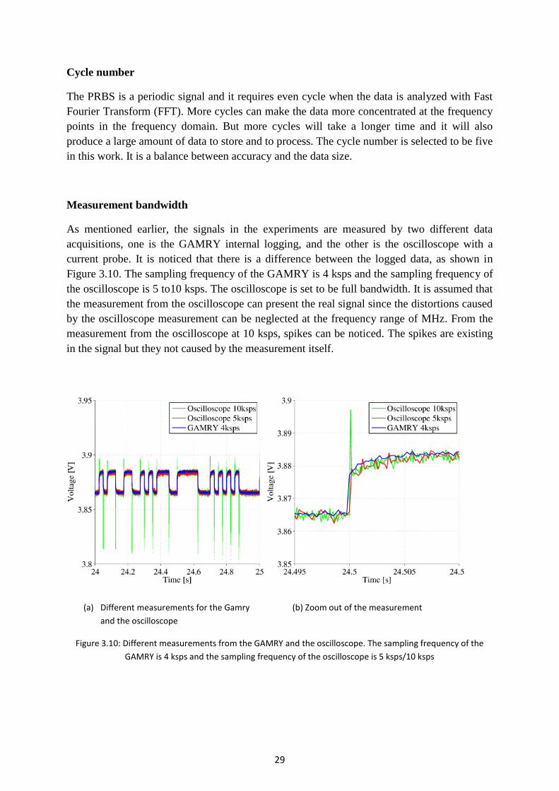
As mentioned earlier, the signals in the experiments are measured by two different data

acquisitions, one is the GAMRY internal logging, and the other is the oscilloscope with a

current probe. It is noticed that there is a difference between the logged data, as shown in

Figure 3.10. The sampling frequency of the GAMRY is 4 ksps and the sampling frequency of

the oscilloscope is 5 to10 ksps. The oscilloscope is set to be full bandwidth. It is assumed that

the measurement from the oscilloscope can present the real signal since the distortions caused

by the oscilloscope measurement can be neglected at the frequency range of MHz. From the

measurement from the oscilloscope at 10 ksps, spikes can be noticed. The spikes are existing

in the signal but they not caused by the measurement itself.

(a) Different measurements for the Gamry (b) Zoom out of the measurement

and the oscilloscope

Figure 3.10: Different measurements from the GAMRY and the oscilloscope. The sampling frequency of the

GAMRY is 4 ksps and the sampling frequency of the oscilloscope is 5 ksps/10 ksps

30

It shows that there is a low-pass filter or some other kinds of filter inside the GAMRY

measurement. The detailed information is not available from the data sheet. However, the

GAMRY measurements give better results compared to the oscilloscope measurements.

Therefore, the results shown in Chapter 5.1 are from the GAMRY measurements. The

oscilloscope measurements are mainly used to analysis the data since it can sample much

faster than the GAMRY. In theory, the measurements from the oscilloscope can achieve the

same result by applying some digital filters. Due to the time limitation, this is not

implemented in this thesis.

Measurement resolution

In normal commercial data acquisition systems, 12-bit or 16-bit analog to digital converters

(ADCs) are widely used. A higher bit ADC gives a higher resolution but adds additional cost.

For the selected cell, the voltage range is 3.0 V to 4.15 V and the voltage change caused by a

10 A PRBS current is 10 mV. The 12-bit ADC shows a poor result while the 16-bit ADC

performs better, as shown in Fig. 3.11. Therefore, in other measurements from the

oscilloscope the 16-bit ADC is always used.

(a) Measurements with different resolutions (b) Zoom out of the measurements

from the oscilloscope

Figure 3.11: Measurements from 12-bit and 16-bit ADCs from the oscilloscope

This should be taken care of when the measurement is performed on the vehicle level. If a 16-

bit ADC is used to measure voltage on the battery pack on the vehicle whose rated voltage is

around 600 V, the resolution is

31

Whether this resolution is sufficient depends on the impedance of the battery pack and the

input current signal.

Sampling frequency

According to the Nyquist-Shannon sampling theorem [35], if a signal contains no higher

frequency than f, a sufficient sampling frequency is 2f. Equivalently, a sampling frequency

can properly determine the characteristics of a signal. However in reality, the sampling

frequency needs to be much higher than the Nyquist sampling frequency, maybe more than 10

times, to achieve good results. Low sampling frequency will cause phase shift and possible

aliasing signal [35]. The clock frequency of the PRBS is 40 Hz.

The phase shift caused by the sampling frequency can be seen in Fig. 3.12.

Figure 3.12: EIS measurement with different sampling frequency showing the phase shift

The phase shift can be analyzed easier in the bode plot in Fig. 3.13. As can be seen that with

the sampling frequency reducing, the amplitude of the impedance can still be identified

properly but the phase starts to shift. The phase shift is larger at the higher frequency range.

Both figures 3.12 and 3.13 are from the GAMRY measurement.

32

Figure 3.13: EIS measurement with different sampling frequency in Bode plot showing the phase shift

The parameters selected in the PRBS method are summarized in table 3.3.

Table 3.3: Summary of parameters for the method validation of the PRBS

3.2 Simulation setup

As in the battery model implementation, engineering software such as Matlab and Simulink

has been used for the creation of simulation algorithms and models that will aid the progress,

goals and completion of this Master Thesis. The aim is to simulate as accurately as possible

the results from the lab experiments. It is also essential to do it in the simplest and most user-

friendly way possible, run the experiments, validate data and compare results.

33

The simulation of both the EIS and PRBS signals on a battery cell and on the electric drive

line serves the purpose of method validation. The EIS method is used as a reference and the

findings of the PRBS are compared to those of the EIS reference. The validation can save a

lot of time, especially in cases in which electrical components are simulated through various

parameters and variables. The simulation model aims at speeding up the procedures of

examining all the required experiments for the thesis work and for any future work on the

subject.

For both EIS and PRBS battery models, the EIS and the PRBS are the current input in the

battery, and a suitable algorithm has been implemented for the control of the simulations. The

algorithms give ease of use also due to the fact that all important parameters can be altered

and their effect examined from there.

All algorithms that were implemented along with the setup of the parameters used for the

simulations are to be found in the Appendix, section Simulation Algorithms.

35

4. Implementation in the vehicle

To perform a PRBS measurement on the battery pack in an EV or an HEV, a PRBS current

need to be generated and applied on the battery. Instead of using any additional equipment,

the existing driveline of the vehicle can be used to perform an onboard test. The electric motor

is chosen as the load to generate the PRBS current since it is more controllable and has a

faster response compared to other loads. A simulation is made to examine to possibility of

having a PRBS current by controlling the electric motor.

4.1 Motor model and control algorithm

The electric motor used in the simulation is a permanent magnet synchronous motor (PMSM)

and the field oriented control (FOC) with field weakening is used to control the motor. The

dynamic model of a PMSM and the FOC are described in the sections to follow.

4.1.1 Motor model

The PMSM consists of a rotor built with permanent magnets to provide the magnetic field.

The windings are distributed in the stator and fed with a three-phase voltages. The voltage and

current in the stator can be presented in αβ-coordinates in order to simplify the analysis. An

amplitude invariant transformation is shown in equation 4.1. The transformation is a

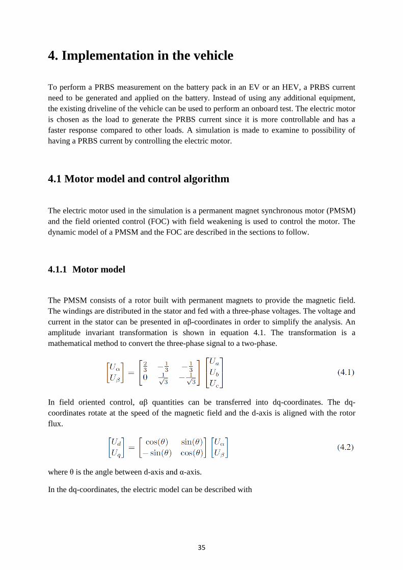
mathematical method to convert the three-phase signal to a two-phase.

In field oriented control, αβ quantities can be transferred into dq-coordinates. The dq-

coordinates rotate at the speed of the magnetic field and the d-axis is aligned with the rotor

flux.

where θ is the angle between d-axis and α-axis.

In the dq-coordinates, the electric model can be described with

36

where is the speed of the flux linkage [45].

The mechanical model is presented by

where is the electric torque produced by the motor and is the load torque. The

mechanical damping is represented by .

The meaning and value of other parameters are shown in Table 4.1. The value of the

parameters are from the simulation model of the Volvo Prototype Machine (VPM). The

parameters J and b is for a stand-alone PMSM, i.e. not mounted in the vehicle.

Table 4.1: Motor parameters used in the simulation from Volvo Prototype Machine (VPM)

4.1.2 Motor controller

In an EV/HEV the electric motor is typically involved in the propulsion of the vehicle. The

electric motor is commanded to generate a required torque which is calculated with the

position of the gas pedal. The electric torque produced by the motor is related to the stator

current, as shown in equation 4.3. Accordingly, a very important part of the motor controller

is the current controller, which is shown in Fig. 4.1.

37

Figure 4.1: A block diagram of the basic close loop motor controller

The idea of the controller is to make the close loop system to be a first-order low-pass filter

[46]. So the current controller has the same bandwidth as which represent the PMSM.

This forms a PI controller

where the two parameters and are the proportional gain and the integral gain. They can be

calculated based on the motor parameter, the bandwidth of the controller.

The controller bandwidth is chosen to be 732 rad/s which is designed by Volvo.

As the motor speed increases, the stator voltage reaches its maximum value, which is limited by the

output voltage of the battery. If a higher speed is required, a field weakening control needs to be

implemented. The field weakening is obtained by ordering a negative d-axis current reference. More

details about the field weakening are discussed in [46].

In many HEVs/EVs, the electric motors are not only used for the propulsion, but also as generators to

collect the energy during the regenerative braking. The electric motor operates as a generator,

converting the mechanical energy into electric energy. It helps the vehicle to brake and at the same

time, the current is fed back to the battery which charges the battery. During this process, the motor

is given a negative torque reference, which is equivalent to a negative current reference.

4.2 Simulation of the PRBS on the driveline

The simulation model is based on an assignment from the course ENM075 Electric drives 2,

at Chalmers University of Technology. The simulation is performed with the use of

MATLAB and Simulink. It consists of a battery model, a three-phase inverter, an electric

motor, a motor controller and a modulator, as shown in Fig. 4.2.

38

Figure 4.2: A schematic of the driveline in an electric vehicle

4.2.1 Simulation model of the driveline

The battery model is a constant voltage source with an internal resistor. During the short

simulation time, it is assumed that the battery SOC level does not change accordingly and the

open circuit voltage is constant. For the whole driveline simulation, the voltage deviation on

the battery pack can be simplified to be the voltage drop over a resistance. Compared to a

simplified battery model, an accurate battery model will not affect the motor behavior much

but it will increase the computation load. This is the reason behind the choice of use of a

simplified battery model in this simulation.

The inverter contains six switches which are assumed to be ideal. The switching behavior,

including turn-on time and turn-off time, are ignored. The DC-link capacitor is taken into

consideration since it will eliminate the high frequency components in the battery current. The

inductance in the cable, which connects the inverter and the battery, will have a similar effect

as the DC-link capacitor. However it slows down the simulation speed a lot so it is not

verified in this thesis due to the time limitation.

39

The motor model is implemented by Volvo in dq-coordinates with the parameter values

mentioned above.

As discussed earlier, the motor controller is using FOC with field weakening. A discrete

simulation is used and the sampling time is 8 kHz, the same as the switching frequency in the

inverter. In most of the vehicles, there is a slew rate limitation of the torque outside the

current controller so that the torque of the vehicle will not change too rapidly. Since the

detailed data are not available, it is assumed that there is no limitation on the torque step in the

simulation.

The purpose of the simulation is to apply a PRBS-like current on the battery pack. If the

battery pack voltage is assumed to be constant, there will be a power PRBS applied on the

battery.

Therefore, the torque reference that is sent to the controller is

Finally, a pulse-width modulation (PWM) is used in the modulator to control the switches in

the inverter. The important parameter values in the simulation are listed in Table 4.2.

Table 4.2: Drive line parameters and control parameters used in the simulation

4.2.2 Speed operation range

During the PRBS measurement, the vehicle is assumed to be in the garage and in neutral

position. The electric motor is only attached with the clutch which adds about 50% of the

inertia. The inertia is very small and the speed of the motor can be easily changed using a

small torque so the PRBS power signal cannot be too large otherwise the motor will

accelerate too much that the speed is out of the operation range.

40

On the other hand the PRBS power signal needs to be as large as possible to achieve a high

current on the battery since a good signal-to-noise ratio (SNR) needs to be reached in both the

current and voltage signals with the small impedance of the battery.

The torque/speed and power/speed curves are shown in Fig. 4.3. The idea is to keep the motor

operating under maximum possible torque and speed range to reach the maximum possible

power. During the operation range, field weakening may occur depending on whether the

voltage limitation is reached.

Figure 4.3: The Torque/Speed and Power/Speed curve of the PMSM

4.2.3 Parameters selection of the PRBS in the driveline simulation

Desired Frequency Range

The first step is to select the desired frequency range. An assumption to be made is that the

testing object is of the same chemistry as the battery cell used in the previous experiment. So

the interesting frequency point is around 1 Hz. To capture the charge transfer resistance, the

desired frequency is selected to be 0.2 Hz. The frequency resolution is the same as the lowest

frequency point, as shown in equation 2.5.

The second step is to select the desired highest frequency while the highest usable frequency

in the PRBS is only dependent on the clock frequency, shown in equation 2.4. There are

several factors that limit the slew rate of the current steps in the driveline simulation,

including the bandwidth of the current controller and the DC-link capacitor. Other factors like

41

for example the torque step limitation and the cable inductance, will have similar effects but

they are not included in this simulation. The reasons are explained in the previous section.

Due to these limitations, the clock frequency of the PRBS is preferred to be as low as possible

so that the slow slew rate can be neglected. On the other hand, the clock frequency needs to

be high enough to offer a sufficient frequency range that can be used for impedance

identification.

PRBS bit and cycle number

After the lowest frequency point and the clock frequency are defined, the PRBS bit length can

be calculated based on equation 2.3. A 6-bit PRBS is decided to be used in the driveline

simulation. Three cycles of the PRBS are simulated due to the computation load, more cycles

can improve the result but it is not a key factor in this simulation.

PRBS offset and initial state

In the experiments, a bipolar PRBS is used to avoid an OCV and SOC level deviation.

However, in the driveline simulation the motor is not running in an ideal environment. With a

bipolar PRBS, no power flows from the battery to the motor and the motor speed will

decrease due to mechanical damping. Therefore, a certain offset in the bipolar PRBS is

necessary in order to keep the motor running at a certain speed range.

Another factor is the PRBS initial state. In this thesis, the PRBS is generated by the linear

shift registers and there is an initial value in each register. By default, all the initial values are

set to 1. In this case, the motor will keep accelerating in the first several clock periods and this

is the longest acceleration time during the PRBS test, which limits the initial speed of the

motor and the power amplitude. This long acceleration time can be interrupted by starting the

PRBS at one of the middle states.

After all, since the power amplitude, the PRBS offset and the initial PRBS state are coupled

between them, it is very hard to decide their values through calculation. An arbitrary way to

decide these parameters is by tuning them to get a set of values. To save simulation time, a

simplified simulation is used as shown in Fig. 4.4. The electric model of the motor is

neglected since its time constant is much faster than the mechanical time constant. Only

equation 4.4 is implemented in the motor model, which reduces most of the computation load.

42

Figure 4.4: A simplified mechanical motor model to define the speed operation range and power amplitude for

the PRBS test

Two sets of parameters will be used in the simulation according to the results of the tuning in

the simplified model, shown in Tables 4.3 and 4.4. The setup 1 is aiming towards having the

maximum power amplitude while the setup 2 is based on avoiding the field weakening. The

reason and its analysis will be explained in the results chapter.

Table 4.3: Setup 1 of PRBS parameters used in the drive line simulation with high power amplitude

Table 4.4: Setup 2 of PRBS parameters used in the drive line simulation with high power amplitude

4.3 Results and analysis

The results from the simulations of the PRBS excitation signal on the drive line are presented

in the following section. Both of the setups in Tables 4.3 and 4.4 are examined.

43

Results of the set-up with low power amplitude

With the low power amplitude 2.5 kW, the motor is running in a speed range between 600 and

3000 rpm with an initial speed of 2000 rpm. During the simulation, the excitation signal is

repeated for three cycles and the offset can be used to support the motor to keep running in

this speed range.

Figure 4.5: Operation speed range during the simulation with 2.5 kW power amplitude

The current on the DC side of the inverter and the current on the battery pack are shown in

Fig. 4.6. The DC-link capacitor limits the rise time of the current steps and eliminates the high

frequency components.

Figure 4.6: The DC-link current and battery pack current during the simulation with 2.5 kW power amplitude

44

As discussed before, a good PRBS signal requires sharp current steps but unfortunately there

are a lot of factors that limit the rise time of the current steps in the drive line. In Figure 4.7, a

current step is presented and the rise time is about 2 ms. This value will be even longer if the

cable inductance and the torque limitation are taken into consideration.

Figure 4.7: A zoom of the DC-link current and battery pack current during the simulation showing the rise up

time

The excitation current signal in frequency domain is shown in Fig. 4.8. It looks very similar to

the PRBS signal in frequency domain and it contains signal in the desired frequency range

which is between 0.2 Hz and 5 Hz. The maximum current amplitude is around 1 A. For a

battery pack, whose impedance is several hundreds of mΩ, this 1 A current may cause a

voltage change less than 1 V, which is very hard to measure on a 600 V battery pack,

therefore a high current amplitude is needed.

Figure 4.8: The Fast Fourier Transform (FFT) of the simulated excitation current signal on the battery pack with

2.5 kW power amplitude

45

Results of the set-up with high power amplitude

With a power reference and higher amplitude of 4 kW, a higher current can be achieved in/out

of the battery pack and accordingly the motor is running in a wider speed range which is

between 750 rpm and 3800 rpm, as shown in Fig. 4.9.

Figure 4.9: Operation speed range during the simulation with 4 kW power amplitude

When the motor is running at a high speed, it may operate under field weakening when the

stator voltage reaches the battery output voltage. It can be observed based on the stator current

in d-axis in Fig. 4.10. The d-axis current is negative when the field weakening occurs.

Figure 4.10: The stator current in d-axis and q-axis during the simulation with 4 kW power amplitude. The d-

axis current is negative when field weakening occurs

46

The control method with the field weakening allows the motor to operate in a wider speed

range but on the other hand it introduces more harmonics in the battery pack current, which

can be seen from Fig. 4.11. The battery pack current starts to spread when the field weakening

occurs.

Figure 4.11: The DC-link current and battery pack current during the simulation with 4 kW power amplitude

With more harmonics, the excitation current signal in frequency domain in Fig. 4.12 is a bit

distorted compared to the FFT of an ideal PRBS. However, the maximum current amplitude is

around 1.7 A which is slightly higher than the previous case but still quite low.

Figure 4.12: The Fast Fourier Transform (FFT) of the simulated excitation current signal on the battery pack

with 4 kW power amplitude

47

From the simulations on the drive line, it is found that an excitation current signal is possible

to be generated by the electric motor. This excitation signal is similar to an ideal PRBS and it

can be used to identify the battery pack ipedance. However, due to the controller bandwidth

and the DC-link capacitor, only an excitation signal with a low clock frequency can be

generated. The signal with a high clock frequency might be possible to be generated if the

inverter is controlled as a buck converter, which in turn means that in this case the motor will

be used only as an inductive load. What is more, the currents in both cases are too small to

identify the impedance of a vehicle battery pack. This can be improved by adding additional

inertia on the motor, for example the transmission and the wheel if the vehicle is lifted.

Both of the battery pack currents in the two cases are applied to a simple battery model like in

Fig. 2.8. The EIS of this battery model is shown in Fig. 4.13. The excitation signal with a

lower amplitude can give a better result in which case the motor is not operating under field

weakening. However, the result will be nonetheless unclear since the signal to noise ratio is

too low in both cases.

Figure 4.13: An example of how the excitation signal can be used for system identification. The battery model

used is a simplified Randles, the result is better if the motor is not running under field weakening

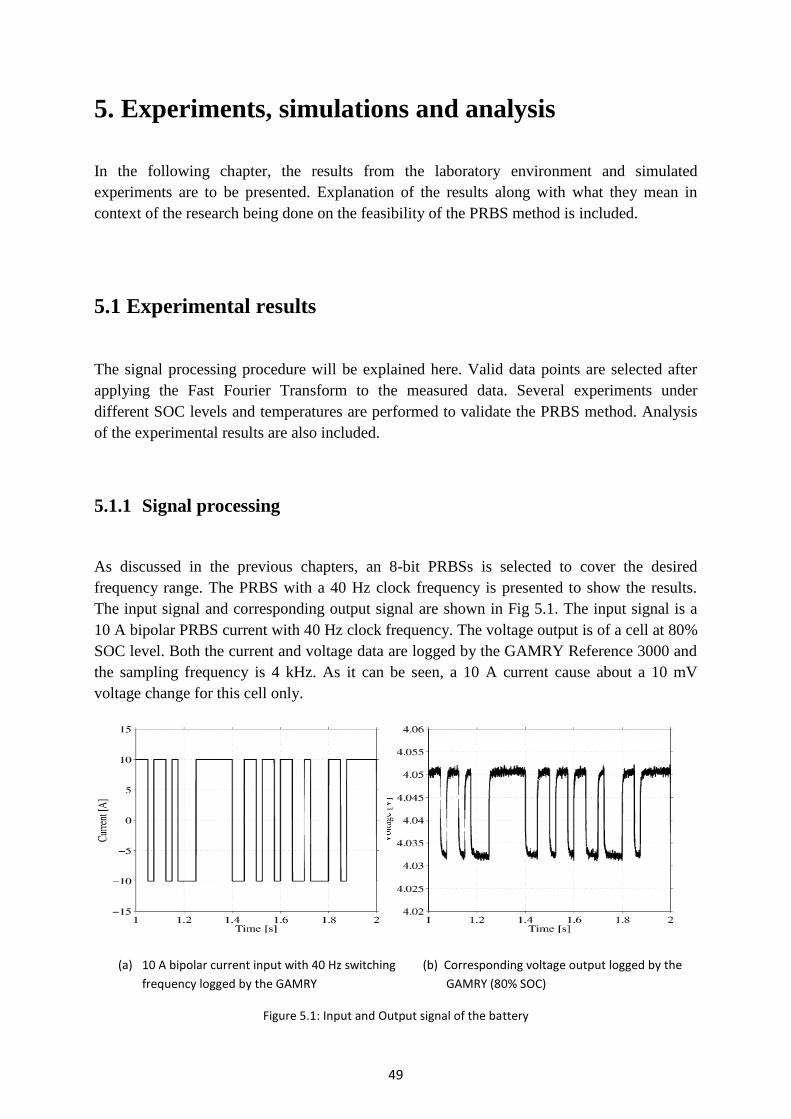
49

5. Experiments, simulations and analysis

In the following chapter, the results from the laboratory environment and simulated

experiments are to be presented. Explanation of the results along with what they mean in

context of the research being done on the feasibility of the PRBS method is included.

5.1 Experimental results

The signal processing procedure will be explained here. Valid data points are selected after

applying the Fast Fourier Transform to the measured data. Several experiments under

different SOC levels and temperatures are performed to validate the PRBS method. Analysis

of the experimental results are also included.

5.1.1 Signal processing

As discussed in the previous chapters, an 8-bit PRBSs is selected to cover the desired

frequency range. The PRBS with a 40 Hz clock frequency is presented to show the results.

The input signal and corresponding output signal are shown in Fig 5.1. The input signal is a

10 A bipolar PRBS current with 40 Hz clock frequency. The voltage output is of a cell at 80%

SOC level. Both the current and voltage data are logged by the GAMRY Reference 3000 and

the sampling frequency is 4 kHz. As it can be seen, a 10 A current cause about a 10 mV

voltage change for this cell only.

(a) 10 A bipolar current input with 40 Hz switching (b) Corresponding voltage output logged by the

frequency logged by the GAMRY GAMRY (80% SOC)

Figure 5.1: Input and Output signal of the battery

50

To prepare the data for the following processing, the first step is to capture only the PRBS

signal to make sure the data is periodic and in an integer amount of cycles. The data during

the rest time needs to be removed. After that, the detrend function in MATLAB can remove a

linear trend of the data which will remove the DC offset. After the preparation, the data is

analyzed in the frequency domain by using the Fast Fourier Transform (FFT).

Since the valid data is located within the 3-dB bandwidth at the specified frequency, the data

need to be selected before calculating the impedance, as shown in Fig 5.2.

(a) FFT of the input current signal and selected (b) FFT of the output voltage signal and selected

current data within the 3-dB bandwidth voltage data within the 3-dB bandwidth

Figure 5.2: Data selection. The valid data is within 3-dB bandwidth

If the selected data are to be put from equation 2.10 to equation 2.11, the impedance

spectroscopy of the battery within the usable frequency range can be calculated. The final

result is shown in Fig 5.3. The EIS presented, is for the selected cell at 50% SOC level.

Figure 5.3: EIS measurement with the PRBS method at 80% SOC level at 0.15 Hz - 15 Hz

51

The blue points are the PRBS measurement and the solid line is the EIS measurement from

the GAMRY Reference 3000 which is a reference. It can be seen that the PRBS points are

distributed along the reference EIS measurement, which means that the PRBS method may be

used accurately to produce an EIS measurement. The PRBS points cover the frequency range

from 0.1568 Hz to 15.8433 Hz, which match the frequency range of interest, calculated in

Table 2.1.

5.1.2 EIS measurement at different SOC level

PRBS measurements are performed at different SOC levels for the same cell. The test

procedure is shown in Fig. 3.2. The results are shown in Fig. 5.4 and Fig. 5.6. The cell is

discharged and charged at 0.5 C by the GAMRY Reference 3000. The PRBS input is a 10 A

bipolar current signal with 40 Hz clock frequency for all the SOC levels. The ambient

temperature is 22°, controlled by a climate chamber. The battery temperature is assumed to be

the same as the ambient temperature since the battery cell has been in the climate chamber for

48 hours before the experiments.

Figure 5.4: EIS measurement with the PRBS method at 0%, 20% and 40% SOC level at 22°

The results show that the PRBS can produce an EIS which is very similar to the reference at

different SOC levels. They also show that the impedance of the battery changes with the SOC

level. The crossing of the X axis Z real, which indicated the ohmic resistance maintains the

same value 0.57 mΩ at differenτ SOC levels. While the charge transfer resistance increases as

52

the SOC level decreases. The values of the charge transfer resistance at different SOC levels

are listed in Table 5.1.

Table 5.1: The values of the charge transfer resistance at different SOC levels

The values that are listed in table 5.1 are plotted in Fig. 5.5 and it can be observed from both

Figures 5.4 and 5.5, the variation of the charge transfer resistance can be more easily detected

at lower SOC levels.

Figure 5.5: The variation of the charge transfer resistance with the SOC level

Apart from the value of the charge transfer resistance, the frequency where it is located is also

an interesting point to investigate. The information about the frequency come from the

standard EIS measurement since the PRBS measurement only covers a limited frequency

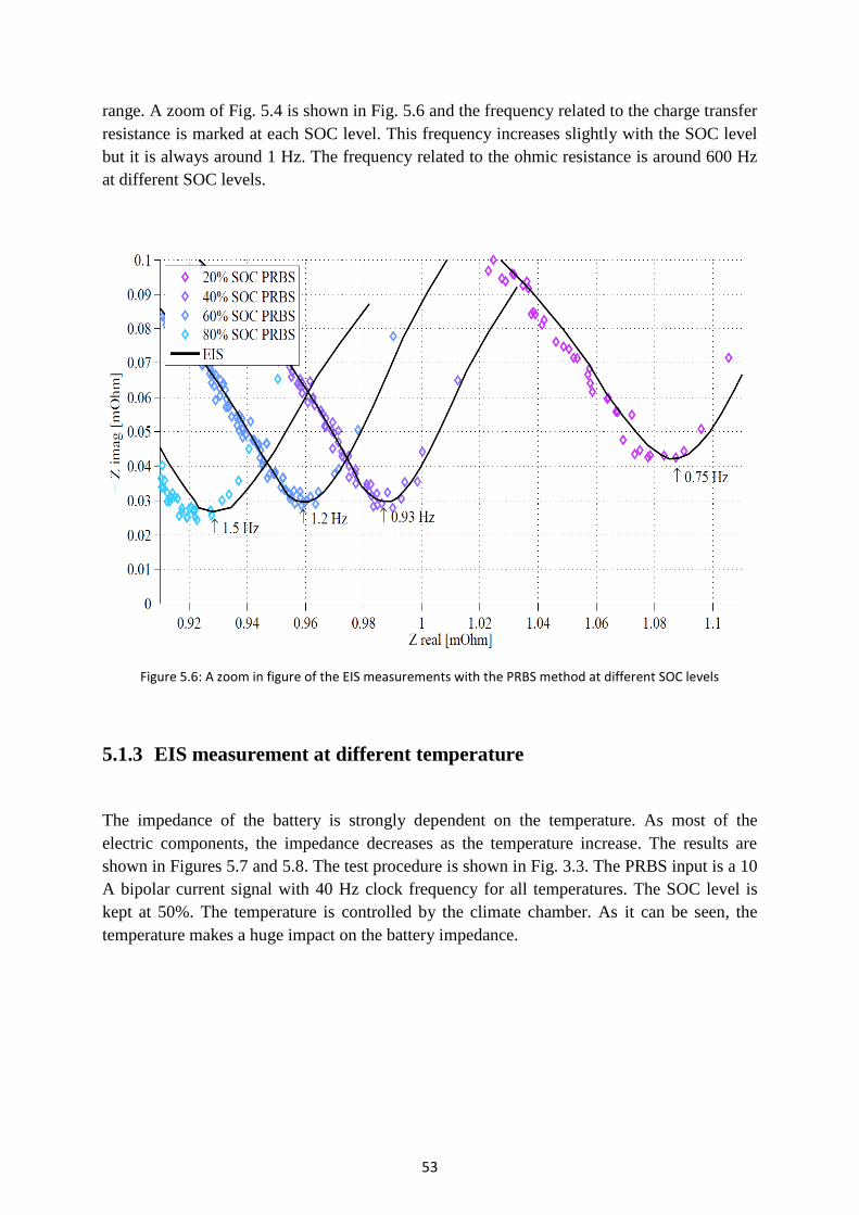
53

range. A zoom of Fig. 5.4 is shown in Fig. 5.6 and the frequency related to the charge transfer

resistance is marked at each SOC level. This frequency increases slightly with the SOC level

but it is always around 1 Hz. The frequency related to the ohmic resistance is around 600 Hz

at different SOC levels.

Figure 5.6: A zoom in figure of the EIS measurements with the PRBS method at different SOC levels

5.1.3 EIS measurement at different temperature

The impedance of the battery is strongly dependent on the temperature. As most of the

electric components, the impedance decreases as the temperature increase. The results are

shown in Figures 5.7 and 5.8. The test procedure is shown in Fig. 3.3. The PRBS input is a 10

A bipolar current signal with 40 Hz clock frequency for all temperatures. The SOC level is

kept at 50%. The temperature is controlled by the climate chamber. As it can be seen, the

temperature makes a huge impact on the battery impedance.

54

Figure 5.7: EIS measurement with the PRBS method at -10°, 0°, and 10° at 50% SOC level

Figure 5.8: EIS measurement with the PRBS method at 10°, 22°, 35° and 45° at 50% SOC level

From the results it can be found that the frequency related to the charge transfer resistance or

the ohmic resistance are affected more by the temperature than the SOC level. Their values

and their related frequency at different temperatures are listed in table 5.2. Since the

frequency information comes from the standard measurement where the frequency sweep has

a relatively large step at high frequency range, the frequency for the ohmic resistance is of an

approximate value.

55

Table 5.2: The values of the charge transfer resistance and ohmic resistance at difference temperatures with

their related frequency

The values listed above are also plotted with the temperatures in Fig. 5.9. Both the charge

transfer resistance and the ohmic resistance decrease with the increase of temperature while

the charge transfer resistance is more significantly reduced. At higher temperature, the

frequency is higher for the charge tranfer and lower for the ohmic resistance, which means the

semicircle that is between them is covered with a smaller frequency range.

Figure 5.9: The variation of the charge transfer resistance, the ohmic resistance and their related frequency

with the temperatures

56

5.2 Simulation results

The results of the simulation are respectively presented in the following subchapter. The

results include the Nyquist behavior for the implementation of the EIS and PRBS methods

and their comparison as well as a validation tool with the purpose of demonstrating that the

battery model can reproduce an EIS measurement response.

5.2.1 EIS implementation

The EIS method has been implemented for a frequency range of 0.04 to 1000 Hz and is

cooperating with the battery simulation model, described in section 2.3. The signal of the EIS

method is a sinusoidal wave, as seen in Fig. 5.10.

Figure 5.10: Depiction of the EIS signal

If the voltage response is to be added with the EIS current input signal, the phase difference

can be depicted in Fig. 5.11(a). From Fig. 5.11 (b), it is easier to observe the slight difference

between the current and the voltage phase.

57

(a) The total current input and voltage output (b) Closer look at the current and voltage

response of the EIS method phase wave form at a certain time point

Figure 5.11: The current and voltage wave form for a frequency range of 0.04 to 1000 Hz

By having the phase difference, and from the impedance formulae for the real and imaginary

part, the Nyquist plot can be created, Fig. 5.12.

Figure 5.12: Nyquist plot of the impedance, derived by using the EIS method on the battery model, for a

frequency range of 0.04 to 1000 Hz

58

The Nyquist diagram has been plotted for a vast range of frequencies so that it can be used as

a reference tool of the PRBS method for any case needed to be examined and verified. The

shape of the curve is presenting the EIS characteristics of a simple equivalent circuit.

Further result plots of the EIS implementation such as the Bode plot and the frequency-phase

shift plot can be found in the Appendix.

5.2.2 PRBS implementation

The PRBS signal, applied in validation simulations is a square wave signal as described in

section 2.4.2. Using the method depicted in Fig. 2.3 it is created to be random and it can be

seen in Fig. 5.13.

Figure 5.13: Depiction of the PRBS signal used in the battery model

Afterwards, coupling the PRBS signal to the battery model, the voltage response achieved

with the PRBS current input can be seen in Fig. 5.14(a) and the Nyquist plot, Fig. 5.14(b)

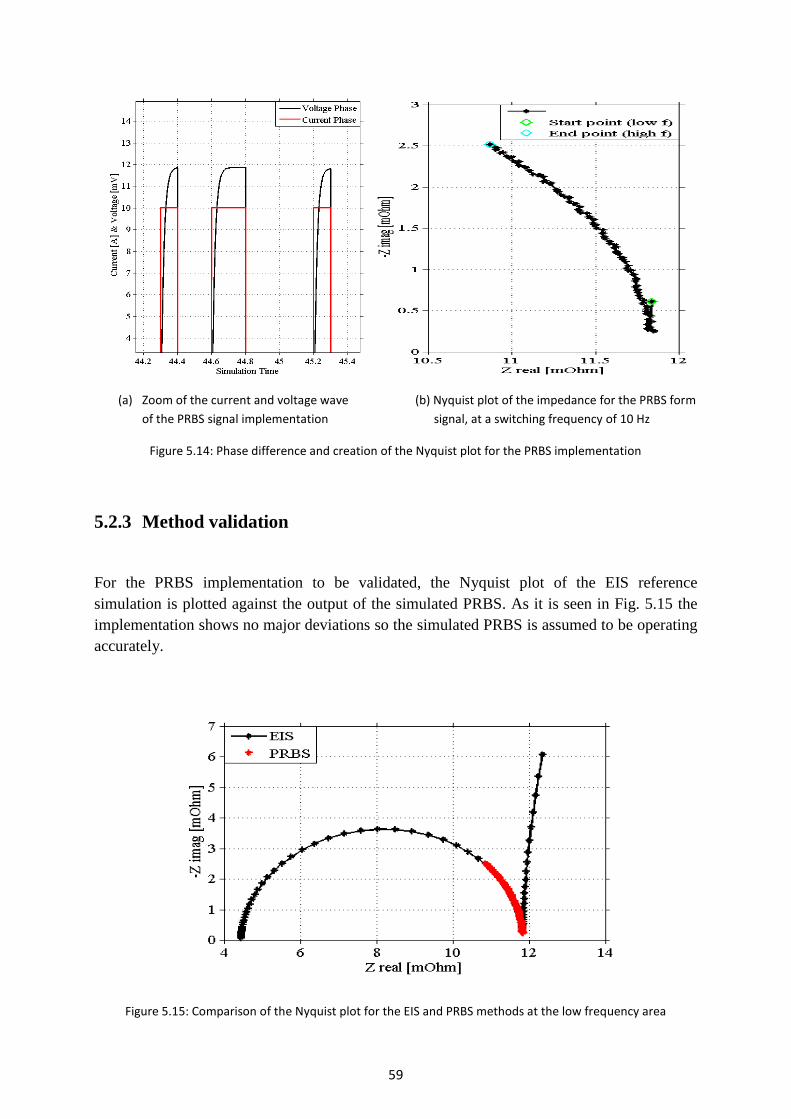
59

(a) Zoom of the current and voltage wave (b) Nyquist plot of the impedance for the PRBS form

of the PRBS signal implementation signal, at a switching frequency of 10 Hz

Figure 5.14: Phase difference and creation of the Nyquist plot for the PRBS implementation

5.2.3 Method validation

For the PRBS implementation to be validated, the Nyquist plot of the EIS reference

simulation is plotted against the output of the simulated PRBS. As it is seen in Fig. 5.15 the

implementation shows no major deviations so the simulated PRBS is assumed to be operating

accurately.

Figure 5.15: Comparison of the Nyquist plot for the EIS and PRBS methods at the low frequency area

60

Influence of noise implementation

What has to be added though in the PRBS signal in order to represent real life conditions

more accurately is noise. The different type of noise to be implemented and examined is white

noise at low and high frequencies and digitalization noise. In addition, a sensitivity analysis of

the boundaries at which the model still operates correctly shall be identified.

For the white noise implementation, a percentage of the current amplitude is added as noise

power and the effect of it is examined.

(a) PRBS signal with 1% white noise (b) Comparison of the EIS and PRBS methods

Figure 5.16: PRBS signal effect and method comparison for a white noise addition of 1%

(a) PRBS signal with 10% white noise (b) Comparison of the EIS and PRBS methods

Figure 5.17: PRBS signal effect and method comparison for a white noise addition of 10%

61

Figure 5.18: Comparison of the EIS and PRBS methods for a white noise addition of 25%

From Figures 5.16(a) and 5.17(a) the effect of the white noise on the PRBS signal can be

observed. Subsequently, Fig. 5.16(b) and 5.17(b) depict the behavior of the PRBS signal in

comparison to EIS reference. Operating above a noise to signal ratio of 25% it can be

observed from Fig. 5.18 that the deviation in the results is becoming higher.

With the same principle in mind, the white noise will be implemented for the high frequency

area of the PRBS signal, that have not yet been tested experimentally in the laboratory

environment due to equipment limitations.

Figure 5.19: Comparison of the EIS and PRBS methods at the high frequency range, no noise implemented

62

(a) 1% white noise implemented at the high (b) 5% white noise implemented at the high

frequency range [1000 Hz] frequency range [1000 Hz]

Figure 5.20: Comparison of the EIS and PRBS methods at the high frequency range for noise implemented

It can be seen in Fig. 5.19 that for no noise implemented in the PRBS, the signal follows the

curvature of the reference almost in a similar manner. The small deviation existing can be due

to minor differences in the method implementation. For a noise to signal ratio addition of 1%

and 5%, depicted in figures 5.20(a) and 5.20(b) accordingly, the noise implementation of 1%

shows an insignificant deviation and remains within the lines of the reference, whereas the 5%

presents significant differences on its response. As an outcome, what can be said that both for

low and high frequency PRBS, the sensitivity response to noise addition is considered to be

the same, especially in the low noise area recommended for further use.

The digitalization noise is implemented with a zero-order hold before each measurement of

the current and voltage data, and for various sampling times that will affect the quality of the

signal. Depicted in Fig. 5.21 is the PRBS signal after being subjected to digitalization noise.

63

Figure 5.21: Depiction of a PRBS signal affected by digitalization noise of 5%

Figure 5.22: Comparison of the normal PRBS signal with the affected by digitalization noise of 5%

In the areas where the original PRBS and the one with the noise do not meet in Fig. 5.22 all

information from the signal are lost. This is the effect this kind of noise can have in the PRBS

signal.

The deviation that can be affected from the digitalization noise can be observed in Fig. 5.23.

64

Figure 5.23: Comparison of the EIS and PRBS methods for digitalization noise implementation

Taking into consideration the results mentioned above and the behavior of the PRBS in

comparison to the EIS, shown in Fig. 5.24, a white noise with a signal to noise ratio of 1%

will be used for further experiments to be simulated for the validation of the PRBS method. A

1% implementation of noise represents a respectable amount of noise in the battery model

implementation but at the same time does not create major deviations in the results.

Figure 5.24: Implementation and comparison of the EIS and PRBS method for the whole frequency range, white

noise addition of 1%

65

Influence of amplitude, SOC, SOH and temperature

For the complete validation of the PRBS method, various parameters such as the SOC, SOH

and more will be examined for different values and their effect in comparison to the reference

will be observed. All parameters to be altered for the simulations to be run can be found in

detail in the Appendix, Table A.2.

The current amplitude, if examined for a range of values, can be observed from Fig. 5.25 that

the PRBS behavior remains significantly parallel to the EIS.

Figure 5.25: Amplitude influence in the PRBS method against the EIS reference in the Nyquist plot, SOC=60%,

SOH=100%, Temperature=20°

The SOC influence can be observed in Fig. 5.26 and Table 5.3. Even though the values of the

charge transfer resistance don’t get such a large impact, nonetheless the influence of the SOC

is visible in it. The closer the values of the SOC are to the reference the closer the charge

transfer resistance is as well.

Table 5.3: Charge transfer resistance influence from SOC

SOC level Charge tranfer resistance

0% 8,8 mΩ

20% 8,4 mΩ

40% 7,8 mΩ

60% 7,4 mΩ

80% 7,6 mΩ

100% 8,05 mΩ

66

Figure 5.26: SOC influence in the PRBS method against the EIS reference in the Nyquist plot, Amplitude=10A,

SOH=100%, Temperature=20°

The same influence can be observed for the SOH, as seen in Fig. 5.27 and Table 5.4. Once

more, and for various SOH values chosen to cover its whole range, the charge transfer

resistance values don’t seem to be changing immensely but despite that, the ones that are

closer to the SOH reference measurement tend to be closer in the resistance values also.

Table 5.4: Charge transfer influence from SOH

SOH level Charge tranfer resistance

0% 8,6 mΩ

30% 6,8 mΩ

60% 6,3 mΩ

100% 7,4 mΩ

67

Figure 5.27: SOH influence in the PRBS method against the EIS reference in the Nyquist plot, Amplitude=10A,

SOC=60%, Temperature=20°

The temperature can be said to be a very important factor when it comes to battery impedance

and this can be observed in the effect it has on the Nyquist plot, depicted in Fig. 5.28.

Figure 5.28: Temperature influence in the PRBS method against the EIS reference in the Nyquist plot,

Amplitude=10A, SOC=60%, SOH=100%

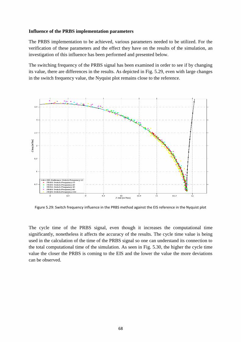
68

Influence of the PRBS implementation parameters

The PRBS implementation to be achieved, various parameters needed to be utilized. For the

verification of these parameters and the effect they have on the results of the simulation, an

investigation of this influence has been performed and presented below.

The switching frequency of the PRBS signal has been examined in order to see if by changing

its value, there are differences in the results. As depicted in Fig. 5.29, even with large changes

in the switch frequency value, the Nyquist plot remains close to the reference.

Figure 5.29: Switch frequency influence in the PRBS method against the EIS reference in the Nyquist plot

The cycle time of the PRBS signal, even though it increases the computational time

significantly, nonetheless it affects the accuracy of the results. The cycle time value is being

used in the calculation of the time of the PRBS signal so one can understand its connection to

the total computational time of the simulation. As seen in Fig. 5.30, the higher the cycle time

value the closer the PRBS is coming to the EIS and the lower the value the more deviations

can be observed.

69

Figure 5.30: Cycle time influence in the PRBS method against the EIS reference in the Nyquist plot

The number of bits affect the quality of the PRBS signal. The purpose of this examination is

to investigate how the PRBS correlates to the reference when its number of bits is decreased

or increased. It can be seen in Fig. 5.31 that for the changes the PRBS was subjected to, the

influence in the results was not that significant and all values could be used for further

simulations.

Figure 5.31: Influence of the number of bits of the PRBS signal against the EIS reference in the Nyquist plot

70

Finally, a parameter such as the cycle time, can increase the computational time significantly

and may affect the results, is the sample time of the EIS and the PRBS. As examined for Fig.

5.32, the increase of the computational time might not be a necessary step due to the fact that

the results produced by it are not significantly different from the ones currently used.

Figure 5.32: Sample time influence in the PRBS method against the EIS reference in the Nyquist plot

Minor deviations in the results along with random points being presented at extraordinary

positions can be justified by implementation differences and noise interactions that affect the

results. The quality of the results nonetheless is considered high, meaning that the validation

of the PRBS method implementation has been completed with the means of the EIS method

as a reference.

What can be said is that in general, the battery model and the implementation in it of the EIS

and most importantly the PRBS method, is operating accurately and as expected. Not only has

the PRBS followed the simulation EIS reference but results and behavior of the same nature

has been observed when the implementation is compared to the laboratory measurements.

Whether it is the noise implementation that affects the impedance and is shown through the

Nyquist plot, as depicted in Fig. 5.1(b) and 5.16(a), or the state of charge, where the similar

behavior can be observed in figures 5.6 and 5.26, or even the temperature, in figures 5.8 and

5.28, a safe assumption is to say that the implementation done in the simulation models for

the operation and validation of the PRBS method produces more than satisfying results and

can be used in any future work on the subject for means of experimentation time save and

more.

71

The influence of parameters may seem to affect the impedance in a different manner than

others. The temperature for instance, has a major effect in the resulted impedance values

whereas the SOC don’t seem to affect it that much. These differences can justified by the fact

that the model implementation, when the SOC is changed the battery operates in a similar

behavior nonetheless whereas when the temperature is changed the whole environment of the

battery operation and subsequently its parameters and results get affected severely. This could

be interpreted as the level of sensitivity that the battery model implementation may show to

various parameters in comparison to others.

Further figures depicting the influence of all the above parameters in their lowest or highest

values used, in addition to their comparison and correlation to the reference method can be

found in the Appendix, section EIS, PRBS and validation figures.

73

6. Conclusions

In this chapter, the results of the investigation along with their outcome is summarized. The

conclusions are presented along with recommendations on how the work could be continued

on the research and investigation of the PRBS method implementation.

6.1 Conclusions from present work

The EIS of the battery depends on the state of charge (SOC), state of health (SOH),

temperature and dynamic state. Therefore, the EIS is a useful tool for the battery. This thesis

focused on the method validation of using PRBS to identify the impedance of the battery. The

investigation proved that the PRBS can be used as a noise signal to measure the

electrochemical impedance spectroscopy (EIS) of the battery in a limited frequency range. It

can give very similar results compared to the measurement from the GAMRY equipment

which uses frequency sweep. The PRBS method is valid at different SOC levels and different

temperature.

This thesis also presented an analysis about how to design a PRBS measurement, including

the selection of the PRBS bit, current amplitude, sign of the signal, rise time of the current

step, cycle number, measurement bandwidth, measurement resolution and sampling

frequency. Both experiments and simulations are performed to analyze the above parameters.

In the conduct of the thesis, an 8-bit design, 5 cycle PRBS current signal with 10 A bipolar is

selected to identify the impedance of the battery. The PRBS method has a good performance

at low clock frequency. However, at high clock frequency the PRBS method shows a poor

result due to the switching spikes caused by the string inductance.

The purpose of investigating the PRBS method is to measure the EIS of the battery pack in

the electric vehicles/hybrid electric vehicles to improve the battery management unit. A

proposal on how to implement the PRBS method is by using the electric motor as the load to

generate the PRBS signal. A simulation is performed to show the driveline behavior during

the PRBS generation.

6.2 Future work

The future work may be divided into two different approaches. First recommendation is to utilize

ways to improve the existing and already tested PRBS method whereas the other method involves

investigation on other ways of implementing the PRBS on the driveline.

74

6.2.1 Improvements for the PRBS method

Due to the low impedance of the battery, the voltage changes are hard to detect. As discussed

in Chapter 3.1.4, a 16-bit ADC has a higher resolution so it can give a better result than a 12-

bit ADC. To increase the resolution more, one way is to use higher bit ADC but it will

increase the cost. Another way is to use a specially designed operation amplifier. The idea of

the amplifier is to remove the DC offset of the signal and increase the scale of the signal.

When designing the op-amp, a stable power source and the isolation need to be taken care of.

According to [23], mixing PRBS signals can improve the bandwidth and noise resilience. It

would be an interesting concept to investigate and if possible to verify it.

As discussed before, the PRBS method shows a poor result with high clock frequency. This

can be improved by a parametric identification. In this approach, a model is required. It can be

a linear model (foster model) or a nonlinear-linear model (Hammerstein-wiener model).

Further investigation is needed.

During the EIS measurement, the signal varies so little in a wide frequency range that a

calibration of the measurement equipment can improve the result a lot. More information is

discussed in [8]. Other than the PRBS method, a multi-sine signal is also a good option for

system identification.

6.2.2 Additional options for PRBS implementation on the driveline

According to the feedback from Volvo buses, other than the ESS, the 24 V lead-acid battery is

also important to have a better SOH diagnostic.

During the driveline simulation, it is assumed that the torque rise up time is mainly limited by

the current controller. However, in reality there is another torque limitation in the automotive

application. Detailed information are not available during the thesis.

In the driveline simulation, the DC-link capacitor plays an important role on how good the

PRBS signal can be. The harmonics are related to the modulation and phase of the motor. It

can be seen from both simulation and real time measurement that when the field weakening

happens, more harmonics are introduced to the DC-link. It would be interesting to study more

on it.

In this thesis, only low clock frequency PRBS is simulated on the driveline by applying a

power PRBS. By the limitation of the current controller, a faster PRBS cannot be achieved.

To generate a high clock frequency PRBS, the inverter can be controlled to be buck converter

and the current can be controlled to follow through the windings without generating torque in

the motor. By performing such an action, it may be possible to have a faster PRBS signal.

75

Bibliography

[1] Yevgen Barsukov, Jinrong Qian. Battery Power Management for Portable Devices.

Artech House, 2013

[2] Jennifer Shuttleworth. Battery Monitoring Unit. SAE International, Automotive

Engineering Magazine, 2010

[3] Anthony C. Fischer-Cripps. The Electronics Companion. CRC Press, 2004

[4] Lakatos John, Oenoki Keiji, Judez Hector et al.. 1998. Learn Physics Today. Lima,

Colegio Dr. Franklin D. Roosevelt

[5] Folker Renken. 1998. Analytic Calculation of the DC-link Capacitor Current for Pulsed

Three-Phase Inverters. Siemens VDO Automotive AG

[6] Oliver Heaviside. The Electrician. AMS Bookstore, 1886

[7] Arthur Kennely. Impedance. AIEE, 1893

[8] Fitzgerald A. E., Charles Kingsley Jr., Alexander Kusko. Electric Machinery, 3rd Edition.

McGraw-Hill, 1971

[9] Siemens CL75 User Manual. Siemens AG. 2005

[10] Lithium-Ion Technical Handbook. Gold Peak Industries Ltd. 2003

[11] The Authoritative Dictionary of IEEE Standards Terms, Seventh Edition. IEEE Press,

2000

[12] Seyed Mohammad Rezvanizaniani, Jay Lee, Zongchung Liu et al.. Review and Recent

Advances in Battery Health Monitoring and Prognostics Technologies for Electric Vehicle

Safety and Mobility. Journal of Power Sources, 2007

[13] Chalasani S. C. Bose, Timothy Beaird. 2002. Battery state of health estimation through

coup de fouet: Field experience. Valence Technology Inc

[14] Demetrius T. Paris, F. Kenneth Hurd. Basic Electromagnetic Theory. McGraw-Hill, 1969

[15] P. Hammond. Electromagnetism for Engineers. Pergamon Press, 1969

[16] E. Barsoukov, J.R. Macdonald. Impedance Spectroscopy: Theory, Experiment and

Applications. Wiley-Interscience, 2005

[17] Mark E. Orazem. 2000. Electrochemical Impedance Spectroscopy. University of Florida

[18] Alan Millner. 2013. Modeling Lithium Ion Battery Degradation in Electric Vehicle.

Massachusetts Institute of Technology

76

[19] Reference 3000 Potentiostat/Galvanostat/ZRA Operator's Manual. GAMRY

Instruments. 2009

[20] VFP600 TM Virtual Front Panel. GAMRY Instruments. 2009

[21] Current Probe Model PR30. LEM

[22] Hideo Okawara. 2013. DSP-Based Testing-Fundamentals 50 PRBS (Pseudo-Random

Binary Sequence). ADVANTEST Corporation

[23] Scott L. Miller, Donald G. Childers. Probability and Random Processes with

Applications to Signal Processing and Communications. Academic Press, 2004

[24] Karl Johan Åström, Richard M. Murray. Feedback Systems-An Introduction for Scientists

and Engineers. Princeton University Press, 2012

[25] Loic Moreau. 2010. Improved Measurement and Analysis Yields Cost-Effective Standby

Battery Monitoring. LEM

[26] Jonathan N. Davidson, David A. Stone, Martin P. Foster et al.. Improved Bandwidth and

Noise Resilience in Thermal Impedance Spectroscopy by Mixing PRBS Signals. IEEE

transactions on power electronics, 2014

[27] Maxime Montaru, Serge Pelissier. Frequency and Temporal Identification of a Li-Ion

Polymer Battery Model Using Fractional Impedance. Les Rencontres Scientifiques de l'IFP -

Advances in Hybrid Powertrains, 2009

[28] E. Kuhn, C. Forgez, P. Lagonotte, G. Friedrich. Modelling Ni-mH battery using Cauer

and Foster structures. Journal of Power Sources, 2006

[29] Avnish Narula. Modeling of ageing of Lithium-Ion batteries at low temperatures. Master

Thesis, Chalmers University of Technology, Gothenburg, 2014

[30] Jens Groot. State-of-Health Estimation of Li-ion Batteries: Cycle Life Test Methods.

Licentiate Thesis, Chalmers University of Technology, Gothenburg 2012

[31] Fairweather, Foster, Stone. MLS testing of VRLA batteries using pseudo-random binary

sequences. World Electric Vehicle Journal, Vol.4, 2010

[32] R. Al Nazer, V. Cattin, P. Granjon et al. Broadband Identification of Battery Electrical

Impedance for HEVs. IEEE transactions on vehicular technology, 2013

[33] Tomi Roinila, Jian Sun. 2013. Online Measurement of Power Grid Impedance.

Rensselaer Polytechnic Institute

[34] Peter Fundaro. 2007. Impedance Track Based Fuel Gauging. Texas Instruments

[35] Tim Wescott. 2015. Sampling: What Nyquist Didn't Say and What to Do About It.

Wescott Design Services

77

[36] R. S. Robinson. System noise as a signal source for impedance measurements on

batteries connected to operation equipment. Journal of Power Sources, 1992

[37] Dinh Vinh Do, Christophe Forgez, Khadija El Kadri Benkara, and Guy Friedrich.

Impedance Observer for a Li-Ion Battery Using Kalman Filter. IEEE transactions on

vehicular technology, 2009

[38] Howey D.A., Mitcheson P.D., Yufit V., Offer G.J., Brandon N.P.. On-line measurement

of battery impedance using motor controller excitation. IEEE transactions on vehicular

technology, 2014

[39] Jürgen Remmlinger, Michael Buchholz, Markus Meiler et al.. State-of-health monitoring

of lithium-ion batteries in electric vehicles by on-board internal resistance estimation. Journal

of Power Sources, 2011

[40] Oliver Bohlen, Stephan Buller, Rik W. De Doncker. Impedance Based Battery Diagnosis

for Automotive Applications. 35th AMWI IEEE Power Electronics Specialists Conference,

2004

[41] Andreas Jossen. Fundamentals of battery dynamics. Journal of Power Sources, 2006

[42] Serial and parallel battery configurations. Battery University. Available:

http://batteryuniversity.com/learn/article/serial_and_parallel_battery_configurations

[43] Allen Fuhs. Hybrid Vehicles: and the Future of Personal Transportation. CRC Press,

2008

[44] H. Helmholtz. Ueber einige Gesetze der Vertheilung elektrischer Ströme in körperlichen

Leitern mit Anwendung auf die thierisch-elektrischen Versuche. Annalen der Physik und

Chemie, 1853

[45] Ramu Krishnan. Permanent Magnet Synchronous and Brushless DC Motor Drives.

Taylor & Francis Inc, 2009

[46] Lennart Harnefors. Control of Variable-Speed Drives. Royal Institute of Technology,

2002

http://batteryuniversity.com/learn/article/serial_and_parallel_battery_configurations

79

Appendix

Specifications

Battery cell specification

Figure A.1: Rechargeable Lithium Ion Battery LQ1729-A1

Table A.1: Battery cell LQ1729-A1 Specifications

80

Simulation Data and Figures

Table of simulation experiments

Table A.2: Table of simulations for the validation of the PRBS method implementation

81

EIS, PRBS and validation figures

Figure A.2: Bode plot of the impedance of the EIS method for a frequency range of 0.04 to 1000 Hz

Figure A.3: Frequency-phase shift plot of the impedance of the EIS method for a frequency range of 0.04 to

1000 Hz

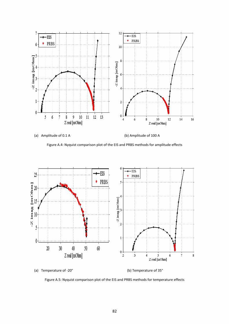
82

(a) Amplitude of 0.1 A (b) Amplitude of 100 A

Figure A.4: Nyquist comparison plot of the EIS and PRBS methods for amplitude effects

(a) Temperature of -20° (b) Temperature of 35°

Figure A.5: Nyquist comparison plot of the EIS and PRBS methods for temperature effects

83

(a) Switch frequency of 5 (b) Switch frequency of 100

Figure A.6: Nyquist comparison plot of the EIS and PRBS methods for switch frequency effects

(a) Cycle time of 1 (b) Cycle time of 10

Figure A.7: Nyquist comparison plot of the EIS and PRBS methods for cycle time effects

84

(a) 6 PRBS bits (b) 14 PRBS bits

Figure A.8: Nyquist comparison plot of the EIS and PRBS methods for effects of number of bits in the PRBS

Figure A.9: Battery simulation model depiction

onboard impedance diagnostics method of li- ion traction

Documents