operational optimization of networks of compressors … · operational optimization of networks of...
TRANSCRIPT

Operational optimization of networks of compressors
considering condition-based maintenance
Dionysios P. Xenosa,∗, Georgios M. Kopanosd,∗, Matteo Cicciottib,c, Nina F.Thornhilla
aImperial College London, Department of Chemical Engineering, Centre for ProcessSystems Engineering, London, UK
bImperial College London, Department of Mechanical Engineering, London, UKcBASF SE, Advanced Process Control, Automation Technology, Ludwigshafen, Germany
dCranfield University, School of Energy, Environmental & Agrifood, Bedforshire, UK
Abstract
The paper presents a mixed integer linear programming optimizationmodel which deals with the optimal operation and maintenance of networksof compressors of chemical plants. This optimization model considers acondition-based maintenance model which involves the degradation of thecondition of the compressors. The paper focuses on online and offline wash-ing, two different cleaning procedures which reduce the extra power used bythe compressors due to fouling. The state-of-the-art has demonstrated theoptimal schedule of the maintenance of a single compressor neglecting theinteractions between operation and maintenance of more than one compres-sor. The suggested optimization model studies a compressor station withmultiple compressors and provides their optimal schedule and the best de-cisions for their washing. Different case scenarios examine the influence ofdifferent types of washing methods on the total costs of operation and main-tenance. The paper demonstrates the benefits of the optimization and provesthat maintenance and operation have to be examined simultaneously and notseparately, in contrast to common industrial practice and previous literature.
Keywords: mixed integer programming, condition based maintenance,washing schedule, compressor washing, fouling
∗corresponding authorEmail address: [email protected] (Dionysios P. Xenos)
Preprint submitted to Computers and Chemical Engineering August 2, 2015

Nomenclature1
Indices/Setse ∈ E products, i.e. O2, N2
i ∈ I compressorsj ∈ J headersn ∈ N process plantst ∈ T time periodsu ∈ U air separation columnsz ∈ Z storage tanks
SubsetsIl large compressorsIs small compressorsINOFF compressors which are not under offline maintenance before
optimizationJ(i) headers connected with compressor i
Subscriptsaux auxiliaryof offlineon online
Superscriptsc cleanmax maximumno nominalo initial state
ParametersCD change header cost [m.u./change]Cf(i) shut down cost [m.u./shut down]Cof(i) offline washing episode cost [m.u./wash]Con(i) online washing episode cost [m.u./wash]CO(e,t) purchase cost of product e in period t [m.u./kg]Cst(i) start up cost [m.u/start up]dc duration of discretized time period [d]
2

doof(i) duration of offline washing of compressor started before opti-mization [d]
doon(i) time period between the latest online washing and the begin-ning of optimization [d]
o(i) maximum running time [d]R recovery factor of online washing model [-]tS number of days before the end of the time horizon [d]WNoel,l/s nominal electrical power of a motor of a large (l) or small (s)
compressor [kW]γ(i) minimum time between two consequent online washing episodes
[d]δSo(i) initial duration of cumulative days of operation before opti-
mization [d]ε(i) degradation rate of compressor i [kW/d]λk minimum number of offline washing episodes [-]λoff maximum number of offline washing episodes in each time pe-
riod [-]λon maximum number of online washing episodes in each time pe-
riod [-]ν(i) duration of maintenance [d]ξ(e,z) capacity of storage tanks [kg]π(i) pressure ratio of compressor [-]ρ(i) mass flow rate of compressor [kg/s]ψ(i) minimum shut down time [d]
ψ(i) continuous offline time before optimization [d]ω(i) minimum online time after the latest start up of compressor i
[d]ω(i) continuous online time before optimization [d]Ω(i) maximum extra power because of degradation [kW]
Continuous non-negative variablesA(e,z,t) amount of product e from storage tank z at t [kg]B(e,z,t) amount of stored product e in tank z at t [kg]C(e,u,t) rate of product e from air separation column u at t [kg/s]L(e,u,z,t) amount of product e from air separation column u provided to
storage tank z at t [kg]M(i,j,t) flow rate of compressed air of compressor i delivered to header
j at t [kg/s]
3

O(e,t) amount of product e purchased from external sources at t [kg]P(i,j,t) discharge pressure of compressor i connected with header j at
t [bar]Wel(i,t) power of a motor of compressor i in period t [kW]W cel(i,t) power consumed when compressor i is not fouled in period t
[kW]∆S(i,t) cumulative time of the operation after the last maintenance of
compressor i at t [d]∆Saux auxiliary variable to linearize the non-linear online washing
model [-]∆Son,aux auxiliary variable to linearize the non-linear combined online
and offline washing model [-]∆W(i,t) extra power consumed from the motor of compressor i at t [kW]
Binary variablesD(i,t) change header status of a compressor i in period tF(i,t) shut down status of a compressor i in period tKof(i,t) finish status of offline washing of compressor i in period tS(i,t) start up status of a compressor i in period tUof(i,t) offline washing status of compressor i in period tUon(i,t) online washing status of compressor i in period tWof(i,t) beginning of offline washing of compressor i in period tX(i,t) operational status of compressor i in period tY(i,j,t) connection between compressor i and header j in period t
4

1. Introduction2
Energy intensive process plants use multiple compressors in parallel to3
increase total available capacity. Spare compressors are used to improve the4
flexibility of the plants and avoid unsatisfied production deliveries, according5
to Kurz et al. (2012). The users of the plants, therefore, have to take decisions6
to optimally exploit this redundancy and coordinate the operation to achieve7
the minimum power consumption and minimum wear of the compressors8
while at the same time the plant meets its production targets in the long9
term. Examples of these decisions are the selection of the online and offline10
compressors.11
Moreover, the maintenance of the compressors increases the complexity12
of the decision-making as more degrees of freedom have to be considered.13
Therefore there is a need for decisions which minimize operational costs,14
increase the lifetime of the compressors and their motors, while also ensuring15
that the plant meets its demand.16
Boyce (2003) explains that the maintenance of a compressor may involve17
several actions such as bearing and rotor repairs, coupling and gear box main-18
tenance, and inspections of the sealings and the motors. The compressors19
which are placed in process gas applications mainly suffer from fouling (Are-20
takis et al., 2012). Fouling is the depositions of particles in the fluid to the21
airfoil. The depositions increase the roughness of the surfaces of the internal22
mechanical components of the compressors (e.g. impeller and diffuser area)23
and restrict the passages areas of the fluid. An example of a fouled impeller24
can be seen in Fig. 1. Thus, the result of the fouling is a decrease in perfor-25
mance and increase in power consumption for the same load compared to a26
Impeller side view Impeller view from the top (side plate removed)
Fouling
Fouling Side plate
Figure 1: Side and top view of a fouled impeller (Forsthoffer, 2011)
5

non-fouled compressor.27
There are two common strategies to deal with the problem of fouling,28
namely offline and online washing. The offline washing takes place when a29
compressor is not operating and the online washing cleans the compressor30
online without interrupting its operation.31
An Offline Washing Episode (OFWE) is complete after several cleaning32
steps when the compressor is in offline mode. The purpose of the washing33
of these cleaning steps is to recover the efficiency of the compressor which34
results in decreasing the extra power consumed. Fabbri et al. (2011) reports35
that supplementary maintenance tasks, such as mechanical and electrical36
inspections, can be included during a typical OFWE, hence the total duration37
of this OFWE can increase up to a few days.38
Another method for improving the performance of a compressor is to in-39
ject a cleaning solution inside the compressor while it is operating online. The40
advantage of this method is that less power is consumed without shutting41
down the compressor to wash. However, the recovery of the performance42
is smaller than in the case of an offline washing episode. Figure 2 shows43
the qualitative trends of the efficiencies when a compressor is not washed,44
is washed online exclusively and is cleaned with offline and online washing.45
According to Fabbri et al. (2011) an Online Washing Episode (ONWE) can-46
not take place if the ambient temperature is less than 14oC because ice is47
created which can damage the blades of the compressor.48
Time
Effi
cien
cy
Ideal maximum efficiency
no washing
only online washing
combined offline and onlinewashing
offline washingstarts
Figure 2: The qualitative trend of the efficiency considering different typesof washing methods.
6
2. Background and context49
In the last half decade there has been interest in the optimization of com-50
pressor stations. Xenos et al. (2015a) presented a survey on the optimization51
of compressor stations in natural gas networks, utilities, gas storage and other52
applications. The key points of the survey were that most of the studies on53
the optimization of compressors focus on the operation of gas networks in-54
cluding compressors and the optimization disregards important aspects of55
operation of compressors such as start up and shut down actions.56
The optimal operation of gas compressors in different process systems57
has been studied by many researchers, for example Sun et al. (2014), Hasan58
et al. (2009) and Han et al. (2004). These researchers employed a steady-59
state optimization analysis (solution for one set of operational conditions)60
compared to the scheduling approach from van den Heever and Grossmann61
(2003). The latter study focused on the pipeline network and not on the op-62
erational aspects of the compressors such as shut down and start up actions.63
Other studies focused on the optimal control of the compressors. These stud-64
ies employed model predictive control strategies and recent examples are the65
papers by Gopalakrishnan et al. (2013) and Zavala (2014).66
There is research on the estimation of the performance of compressors67
considering degradation due to fouling, especially on axial compressors, an68
example is the study from Boyce et al. (2007). There are also many authors69
who studied the performance deterioration of the compressor of a gas turbine70
for power generation. Aretakis et al. (2012) carried out an economic analysis71
of a single gas turbine to estimate the optimal number of the offline washings72
for one year. The authors considered costs such as capital, washing, start73
up and fuel costs. Li et al. (2009) described a prognostic approach to esti-74
mate the remaining time of a gas turbine until its next maintenance episode.75
Other thermodynamic and economic analysis were presented by Sanchez et76
al. (2009) and Fabbri et al. (2011).77
The latter studies did not incorporate maintenance actions into their op-78
timization formulation. Boyce (2003) referred to a concept of integration79
between operation and maintenance, the author called this integration Per-80
formance Based Total Productive Maintenance (PTPM), however this refer-81
ence did not present a method to achieve this integration. Recent works on82
networks of compressors by Kopanos et al. (2015) and Xenos et al. (2015b)83
presented the simultaneous optimization of operation and maintenance. Both84
studies included maintenance tasks which deal with preventive maintenance85
7

tasks, however the cost of the maintenance was not included into the objec-86
tive function.87
There are also papers which studied the maintenance scheduling of single88
or parallel units in other applications such as biopharmaceutical manufactur-89
ing (Liu et al., 2014), wind turbine farms (Gustavsson et al., 2014), process90
plants (Sequeira et al., 2001; Hazaras et al., 2012; Biondi et al., 2015) and91
power plants with gas engines (Castro et al., 2014). The article by Castro et92
al. (2014) deals with the maintenance scheduling of parallel gas engines and93
the work demonstrates many similarities with the topic of the current paper.94
Castro et al. (2014) employed a mixed integer linear programming model95
which considered shut downs and start ups of the engines, and constraints96
which involved industrial restrictions related to maintenance, for example97
where there were limited maintenance resources. However, the model con-98
sidered an industrial case with identical engines and their power consumption99
was independent of time and operational conditions.100
According to the previous statements, the literature from one side exam-101
ines the maintenance of a single compressor considering its performance, and102
on the other side examines the optimization of the operation of networks of103
compressors neglecting their maintenance tasks. Hence, the optimization of104
a compressor station with multiple (not necessarily similar) compressors in105
parallel considering their maintenance is still an open question.106
For these reasons, this work suggests a mathematical framework for the107
optimal operation of a network of compressors considering condition-based108
maintenance. The framework includes a Mixed Integer Linear Programming109
(MILP) model. The model involves the basic operational constraints of the110
compressors considering the prediction of power consumption depending on111
operational conditions, the extra power consumption due to degradation, and112
minimum running and minimum shut down times of the compressors. The113
model also includes the offline and online washing maintenance which is the114
key contribution of the current study.115
Section 3 presents the MILP optimization models including constraints116
for the online, offline and combined washing. Section 4 describes an industrial117
case study of an air separation plant. Section 5 demonstrates and discusses118
the results of the paper and Section 6 presents the conclusions.119
8

3. Methodology120
The paper focuses on the optimal operation of an air separation plant121
which involves an air compressor station. Figure 3 shows a simplified de-122
scription of the plant. The compressor station comprises of multiple com-123
pressors with dissimilar characteristics and they operate in parallel. The air124
compressors can connect with different headers. Moreover, the headers are125
connected with downstream processes, for example air separation columns,126
and process plants which require compressed air for utilities. The air sepa-127
ration columns separate the compressed air into nitrogen, N2, and oxygen,128
O2, which are the main products of the plant. These products can be stored129
in buffer tanks. At the exit of the plant both O2 and N2 are provided to130
internal or external customers, an internal customer may be a process plant131
on the same site which uses oxygen for its own processes.132
i = 1
i = I
Process plant n1utilities
Oxygen storage
1
Oxygendemand
Oxygen storage
2
Oxygen storage
3
Cryogenicprocess
Cryogenicprocess
i = 2
Nitrogenstorage
1
Nitrogendemand
M
M
M
Nitrogen lineOxygen lineAir line
Compressorstation with centrifugalcompressors
Air separation column 1
Air separation column 2
Headers
Figure 3: An air separation plant with an air compressor station.
The proposed optimization framework optimizes the operation and at133
the same time considers a condition-based maintenance model. The pro-134
posed mathematical model is based on the operational model of networks135
of compressors developed by Kopanos et al. (2015). The equations of the136
9

operational model are summarized in Tables 6, 7 and 8 which can be found137
in the Appendix.138
The optimization model of the current framework includes a set of com-139
pressors i ∈ I, a set of headers j ∈ J , a set of air separation columns u ∈ U ,140
a number of tanks z ∈ Z and set of gas products e ∈ E. The optimization141
considers a finite time horizon which is uniformly discretized in time periods142
t ∈ T . The main binary variables used in the optimization problem are pre-143
sented below:144
145
X(i,t) = 1, if a compressor i is operating during time period t,146
S(i,t) = 1, if a compressor i starts up at the beginning of t,147
F(i,t) = 1, if a compressor i shuts down at the beginning of t,148
Y(i,j,t) = 1, if a compressor i is serving header j at the beginning of t,149
D(i,t) = 1, if a compressor i changes header at the beginning of t,150
Wof(i,t) = 1, if a compressor i starts offline washing at t,151
Uof(i,t) = 1, if a compressor i is under offline washing during t,152
Kof(i,t) = 1, if the offline washing of a compressor i has already finished153
at the beginning of t,154
Uon(i,t) = 1, if online washing of a compressor i occurs in time period t.155
156
Sections 3.1 – 3.5 provide the extension of the operational model of the157
compressors implementing the models of the offline, online and combined158
washing maintenance. The combined washing strategy considers the option159
of selecting online or offline washing. The resulting integrated framework160
determines optimal operation and provides the best decisions of the mainte-161
nance tasks.162
3.1. Offline washing maintenance163
Figure 4 illustrates an example of an episode of offline maintenance, i.e.164
offline washing. The offline washing starts at time period t3 and it lasts until165
t5. Therefore, the compressor is available from period t6 and after. In this166
example the compressor remains off for periods t6 and t7 and starts up in167
period t8.168
Equations (1) – (4) connect the basic variables of an Offline Washing169
Episode (OFWE). The duration of an OFWE is described by parameter ν(i)170
and it varies according to the type of the compressor and the supplementary171
maintenance actions that are related to the washing maintenance (e.g. me-172
chanical inspection). When an offline washing episode starts, i.e. Wof(i,t) = 1,173
10

then the compressor must stay offline during this period t, i.e. X(i,t) = 0.174
This is modeled through Eq. (5) which also satisfies the case when a com-175
pressor has to be switched off, i.e. X(i,t) = 0, for reasons other than washing,176
therefore binary variable Wof(i,t) can take the value zero.177
tt1 t2 t3 t4 t5
Com
pres
sor i
1 st
atus
t6 t7 t8
Starts offline washingWof (i1,t3) = 1
Offline washing completesKof (i1,t6) = 1
Under maintenance Uof (i1,t3) = Uof (i1,t4) =Uof (i1,t5) =1
Figure 4: Offline washing episode and binary variables explanation.
The optimization model considers offline washing episodes (OFWEs) that178
occurred before the start of the optimization time window. This information179
is part of the input of the model and describes the initial state of the system.180
The significance of proper consideration of the initial state of the system has181
been highlighted in the work by Kopanos et al. (2014). The parameter doof(i)182
gives the duration of a compressor which has already been in maintenance183
before the beginning of the time horizon of the optimization. If doof(i) > 0184
then the compressor has to continue being maintained up to the time period185
(ν(i) − doof(i)). Equation (6) describes this constraint.186
11

Wof(i,t) −Kof(i,t) = Uof(i,t) − Uof(i,t−1),∀i ∈ I, (doof(i) > 0, (ν(i) − doof(i)) < t ≤ T ) ∨ (doof(i) = 0, t > 1) (1)
Wof(i,t) −Kof(i,t) = Uof(i,t),
∀i ∈ I, doof(i) = 0, t = 1 (2)
Wof(i,t) +Kof(i,t) ≤ 1,
∀i ∈ I, (doof(i) > 0, (ν(i) − doof(i)) < t ≤ T ) ∨ (doof(i) = 0, t ∈ T ) (3)
1− Uof(i,t) +t∑
t′=max1,t−ν(i)+1
Wof(i,t′) = 1,
∀i ∈ I, (doof(i) > 0, (ν(i) − doof(i)) < t ≤ T ) ∨ (doof(i) = 0, t ∈ T ) (4)
X(i,t) ≤ 1− Uof(i,t),∀i ∈ I, t ∈ T (5)
Uof(i,t) = 1,
∀i ∈ I, d0of(i) > 0, 1 ≤ t ≤ (ν(i) − doof(i)) (6)
Equation (7) models the maximum number λoff of maintenance episodeswhich can take place in one time period. The simultaneous maintenanceepisodes in one time period (e.g. in one day) may be restricted due to indus-trial policies.∑
i∈I
Uof(i,t) ≤ λoff , ∀t ∈ T (7)
The constraints described by Eqs. (8) – (12) provide the models of the187
degradation rate and recovery of the extra power consumption after an of-188
fline washing episode. The main assumptions of the degradation and power189
recovery model are summarized below:190
191
1) The degradation rate of a compressor depends on the type of the com-192
pressor and on the cumulative time of operation after the last maintenance.193
A linear function between extra power consumption due to degradation ∆W194
and cumulative operational time ∆S is employed: ∆W(i,t) = ε(i)∆S(i,t), where195
12
ε(i) is the degradation rate of each compressor.196
197
2) It is assumed that the effects from the surroundings do not change abruptly198
during a short time period. For instance, the construction of a new plant close199
to the compressor station might increase the dust intake in the compressors200
and the fouling would increase. The linear correlation between extra power201
consumption and cumulative time period of operation would not hold true.202
An advanced performance monitoring diagnostic tool could deal with this203
problem in a rolling horizon scheduling approach similar to that of Kopanos204
et al. (2015).205
206
3) When a compressor is switched off and remains offline without mainte-207
nance the condition of the compressor stays as it was before the shut down.208
In reality, corrosion can continue between the fouling deposits and the blades,209
also during stand-by of the machine according to Meher-Homji et al. (2001).210
211
4) The additional power consumed due to degradation is assumed constant212
during the period t, and it does not depend on the operating point.213
214
5) When a compressor is washed offline it is assumed that the efficiency is215
fully recovered, in other words the extra power consumption due to degrada-216
tion becomes zero immediately after the washing, see Fig. 2. According to217
Diakunchak (1992) a residual decrement of 1% of the degradation might still218
be observed after offline washing, however for the purposes of the illustration219
of the framework this residual is not modeled.220
221
The assumption of a linear correlation between extra power consumption222
due to the accumulation of fouling and time holds true up to a particular223
amount of fouling (Li et al., 2009). The current paper employs values of the224
degradation rate ε(i) derived from the analysis of Cicciotti et al. (2014) on225
the same air separation case study.226
Although there is not a well defined model of the prediction of the ac-227
cumulation of fouling at the moment, it is possible that parameters apart228
from the cumulative time increase the accumulation of fouling. Sanchez et229
al. (2009) presented a list of factors which influence the build up of fouling,230
however the authors in the same work expressed the fouling accumulation231
as a function of time. Fouling, erosion and corrosion are the main causes of232
increased roughness of the surfaces (e.g. blades surfaces) of the compressors.233
13
This increase in roughness is the major factor of reduced performance. The234
rate at which the performance deteriorates is influenced by a large number235
of factors, this fact makes the prediction of the degradation rate impossible236
without infield observations of past behaviour of the compressor.237
Hence, the main objective of this paper is to show the practical use of238
the framework and its potential use when advanced performance monitoring239
methods and explicit models of the accumulation of the fouling are available240
in the future, therefore the assumption that the extra power consumption241
due to degradation depends on the cumulative time of operation is sufficient242
for the current study.243
Com
pres
sor i
1 st
atus
Case of maintenance: Wof (i1,t3) = 1 X(i1,t3) = 0, ΔS(i1,t3) = 0
Case of continuous operation: Wof (i1,t2 )= 0 , X(i1,t2) = 1, ΔS(i1,t2) = 31 + 1
Case of shut down: Wof (2,3) = 0 , X(2,3) = 0, ΔS(1,2) = 32 + 0
Com
pres
sor i
2
stat
us
tt1 t2 t3 t4 t5 t6 t7 t8
δSo(i1) = 30
δSo(i2) = 30
ΔS(i1,t8) = 1
ΔS(i1,t3) = 0ΔS(i1,t1) = 31
ΔS(i2,t3) = 32ΔS(i2,t1) = 31 ΔS(i2,t8) = 33
ΔS(i2,t2) = 32 ΔS(i2,t4) = 32
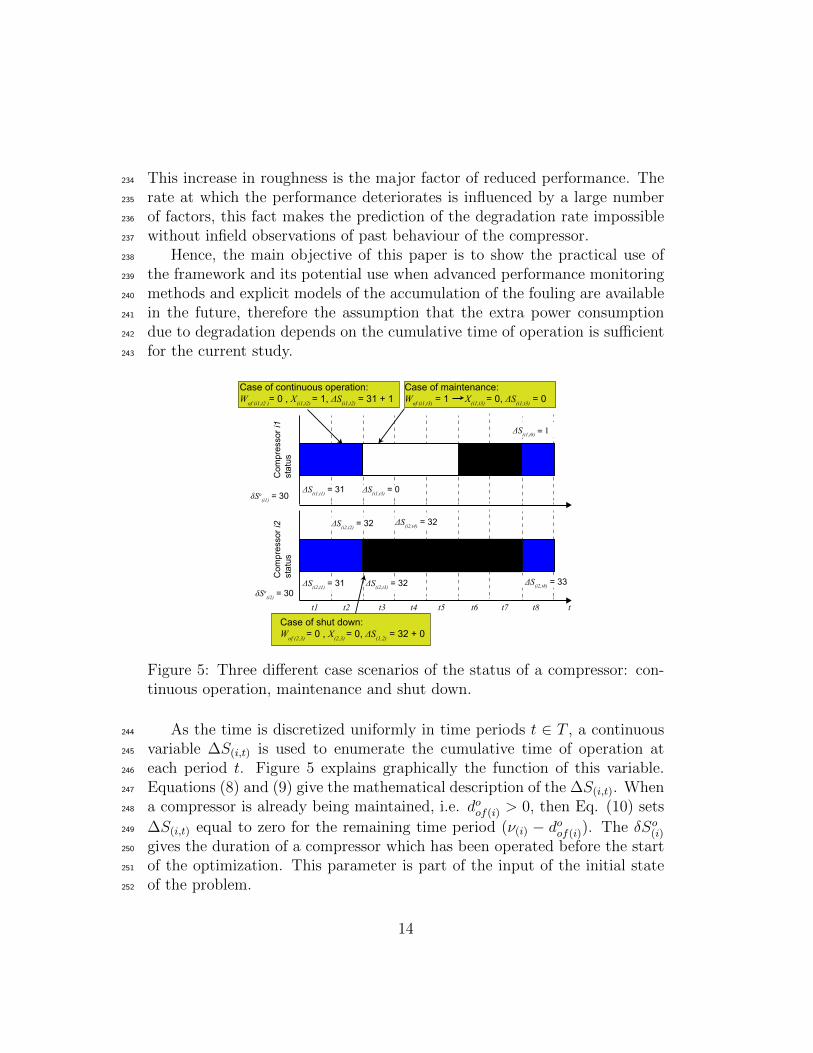
Figure 5: Three different case scenarios of the status of a compressor: con-tinuous operation, maintenance and shut down.
As the time is discretized uniformly in time periods t ∈ T , a continuous244
variable ∆S(i,t) is used to enumerate the cumulative time of operation at245
each period t. Figure 5 explains graphically the function of this variable.246
Equations (8) and (9) give the mathematical description of the ∆S(i,t). When247
a compressor is already being maintained, i.e. doof(i) > 0, then Eq. (10) sets248
∆S(i,t) equal to zero for the remaining time period (ν(i) − doof(i)). The δSo(i)249
gives the duration of a compressor which has been operated before the start250
of the optimization. This parameter is part of the input of the initial state251
of the problem.252
14

∆S(i,t) = (∆S(i,t−1) +X(i,t))(1−Wof(i,t)),
∀i ∈ I, (doof(i) > 0, (ν(i) − doof(i)) < t ≤ T ) ∨ (doof(i) = 0, t > 1) (8)
∆S(i,t) = (δSoi +X(i,t))(1−Wof(i,t)),
∀i ∈ I, doof(i) = 0, t = 1 (9)
∆S(i,t) = 0,
∀i ∈ I, doof(i) > 0 , 1 < t ≤ (ν(i) − doof(i)) (10)
∆W(i,t) = ε(i)∆S(i,t)X(i,t),
∀i ∈ I, t ∈ T (11)
∆W(i,t) ≤ Ω(i),
∀i ∈ I, t ∈ T (12)
Equation (11) gives the expression of the extra power a compressor con-253
sumes because of the degradation. The degradation rate ε(i) depends on the254
size of the compressor. The parameter Ω(i), in Eq. (12), is a maximum255
boundary restricting the extra power consumption due to degradation. This256
parameter is derived from the relationship of the extra power and cumulative257
days, Ω(i) = ε(i)o(i), where o(i) is the maximum running time.258
Equations (8) and (9) involve bilinear terms some comprising multiplica-259
tion of binary with binary variables and others the multiplication of binary260
with continuous variables. The following set of equations, which use the261
principles of the Big-M formulation (Vecchietti et al., 2003), convert these262
nonlinear constraints into linear. The reason is to relax the optimization263
problem and avoid to solve a hard mixed integer non-linear programming264
optimization model.265
15

∆S(i,t) ≤ o(i)(1−Wof(i,t)),
∀i ∈ I, (doof(i) > 0, (ν(i) − doof(i)) < t ≤ T ) ∨ (doof(i) = 0, t ∈ T ) (13)
∆S(i,t) = 0,
∀i ∈ I, doof(i) > 0 , 1 ≤ t ≤ (ν(i) − doof(i)) (14)
∆S(i,t) ≤ δSoi +X(i,t) + o(i)Wof(i,t), ∀i ∈ I, doof(i) = 0, t = 1 (15)
δSoi +X(i,t) − o(i)Wof(i,t) ≤ ∆S(i,t), ∀i ∈ I, doof(i) = 0, t = 1 (16)
∆S(i,t) ≤ ∆S(i,t−1) +X(i,t) + o(i)Wof(i,t),
∀i ∈ I, (doof(i) > 0, (ν(i) − doof(i)) < t ≤ T ) ∨ (doof(i) = 0, t > 1) (17)
∆S(i,t−1) +X(i,t) − o(i)Wof(i,t) ≤ ∆S(i,t),
∀i ∈ I, (doof(i) > 0, (ν(i) − doof(i)) < t ≤ T ) ∨ (doof(i) = 0, t > 1) (18)
Moreover, Eq. (11) involves the multiplication of the continuous variable∆S(i,t) with the binary variable X(i,t). The reason for this multiplication isthat the extra power due to degradation, ∆W(i,t), at a period t should notbe added into the objective function when a compressor i is offline but notwashed. On the other hand, the past time period a compressor has beenoperating has to be registered through ∆S(i,t) for each period t. This leadsto a non-linear equation, where the following formulation can convert theconstraints into linear constraints:
∆W(i,t) ≤ Ω(i)X(i,t), ∀i ∈ I, t ∈ T (19)
∆W(i,t) ≤ ε(i)∆S(i,t) + Ω(i)(1−X(i,t)), ∀i ∈ I, t ∈ T (20)
ε(i)∆S(i,t) − Ω(i)(1−X(i,t)) ≤ ∆W(i,t), ∀i ∈ I, t ∈ T (21)
As discussed in the assumptions, if the model considered the assumption266
of Meher-Homji et al. (2001) that a compressor continues being fouled while267
it is offline, then Eqs. (8) and (9) should exclude the X(i,t) in the first268
parenthesis. This would lead to an easier mathematical problem to solve.269
The current optimization problem considers the case that a compressor is270
not fouled during offline mode.271
16
3.2. Online washing272
The injection of a cleaning solution into the compressor can have un-wanted side effects such as corrosion of the blades if done too frequently. Forthis reason, it is assumed a minimum time period γ(i) of each compressor ibetween two consequent Online Washing Episodes (ONWEs):
Uon(i,t) = 0,
∀i ∈ I, doon(i) < γ(i) , 1 ≤ t ≤ (γ(i) − doon(i)) (22)
t∑t′=maxt−γ(i)+1,1
Uon(i,t′) ≤ 1,
∀i ∈ I, (doon(i) ≥ γ(i), t ∈ T ) ∨ (doon(i) < γ(i), (γ(i) − doon(i)) < t ≤ T ) (23)
Equation (22) is valid when a compressor has been washed online for time273
period doon(i) before the start of the optimization and the doon(i) is smaller than274
the γ(i). For any other case, Eq. (23) holds true.275
Equation (24) describes the fact that there is also a maximum λon ONWEsof different compressors which can take place in each time period of the timehorizon. The reason for considering this constraint is that it is possible theonline washing infrastructure could not support simultaneous online washingas described by Boyce et al. (2007). In any other case, this constraint can beomitted.∑
i∈I
Uon(i,t) ≤ λon, ∀t ∈ T (24)
An online washing episode cannot take place when the compressor isoffline. Equation (25) describes that if a compressor i is online at period t,i.e. X(i,t) = 1, then it has the option to be washed, i.e. Uon(i,t) = 1 or it canbe decided to operate without being washed, i.e. Uon(i,t) = 0. However, if thecompressor is offline, i.e. X(i,t) = 0, variable Uon(i,t) has to be equal to zeroin this time period.
Uon(i,t) ≤ X(i,t), ∀i ∈ I, t ∈ T (25)
The recovery model for online washing, which is described in Eqs. (26)and (27), assumes that ∆S(i,t) is reduced by a recovery factor R. For instance,if the recovery factor is R = 0.2 and the operating period is ∆S(i,t) = 100 d,the final operating period after an online washing would be ∆S(i,t) · (1−R) =
17

80 d. Then the ∆W(i,t) is estimated based on the duration of this period. Thevariable ∆S(i,t) represents the Equivalent Operating Time (EOT) presentedby de Backer (2000) and Bohrenkamper et al. (2000). The online washingmodel completes with the consideration of the degradation model, which isthe same one considered in the case of the offline washing in the previousSection 3.1 and it is defined by Eqs. (11) and (12).
∆S(i,t) = (∆S(i,t−1) +X(i,t))(1−R · Uon(i,t)), ∀i ∈ I, t > 1 (26)
∆S(i,t) = (δSoi +X(i,t))(1−R · Uon(i,t)), ∀i ∈ I, t = 1 (27)
The formulation of the constraints in Eqs. (26) and (27) shows thatthe multiplication of binary and continuous variables is more complicatedcompared to the corresponding case of the offline washing. To overcomethis complexity, the linearization of these constraints employ an auxiliaryvariable ∆Saux(i,t). The linearized constraints of Eqs. (26) and (27) can beseen below:
∆S(i,t) = (δSoi +X(i,t))−∆Saux(i,t), ∀i ∈ I, t = 1 (28)
∆S(i,t) = (∆S(i,t−1) +X(i,t))−∆Saux(i,t), ∀i ∈ I, t > 1 (29)
∆Saux(i,t) = 0,
∀i ∈ I, doon(i) < γ(i), 1 ≤ t ≤ γ(i) − doon(i) (30)
∆Saux(i,t) ≤ o(i)Uon(i,t),
∀i ∈ I, (doon(i) ≥ γ(i), t ∈ T ) ∨ (doon(i) < γ(i), t > (γ(i) − doon(i))) (31)
∆Saux(i,t) ≤ (∆S(i,t−1) +X(i,t))R + (1− Uon(i,t))o(i),∀i ∈ I, (doon(i) ≥ γ(i), t > 1) ∨ (doon(i) < γ(i), t > γ(i) − doon(i)) (32)
(∆S(i,t−1) +X(i,t))R− (1− Uon(i,t))o(i) ≤ ∆Saux(i,t),
∀i ∈ I, (doon(i) ≥ γ(i), t > 1) ∨ (doon(i) < γ(i), t > γ(i) − doon(i)) (33)
∆Saux(i,t) ≤ (δSoi +X(i,t))R + (1− Uon(i,t))o(i),∀i ∈ I, doon(i) ≥ γ(i), t = 1 (34)
(δSoi +X(i,t))R− (1− Uon(i,t))o(i) ≤ ∆Saux(i,t),
∀i ∈ I, doon(i) ≥ γ(i), t = 1 (35)
The degradation model used in the online washing considers the lineariza-276
tion of the constraint of Eq. (11) which was described earlier when discussing277
18

Eqs. (19) – (21) exactly as in the case of the offline washing degradation278
model.279
3.3. Combined online and offline washing280
Section 3.3 describes the scenario when offline and online washings are281
available to clean the compressors. In this case, the optimization model282
employs all the binary variables Wof(i,t), Uof(i,t), Kof(i,t) and Uon(i,t). The283
optimization model includes the constraints in Eqs. (1) – (7) from the offline284
washing formulation in Section 3.1 and the constraints in Eqs. (22) – (25)285
from the online washing model in Section 3.2.286
The degradation and recovery model is a combination of the two differentwashing models. This combined model is described by the constraints in thegeneral form in Eqs. (11) – (12) and the linearized form in Eqs. (19) – (21).The recovery model in the combined online and offline washing scenario isgiven by Eqs. (36) and (37).
∆S(i,t) = (∆S(i,t−1) +X(i,t))(1−Wof(i,t))(1−R · Uon(i,t)),∀i ∈ I, t > 1 (36)
∆S(i,t) = (δSoi +X(i,t))(1−Wof(i,t))(1−R · Uon(i,t)),∀i ∈ I, t = 1 (37)
Equations (36) and (37) can be linearized with the use of an auxiliaryvariable ∆Son,aux(i,t) as follows:
∆S(i,t) ≤ o(i)(1−Wof(i,t)),
∀i ∈ I, (doof(i) = 0, t ∈ T ) ∨ (doof(i) > 0, t > (ν(i) − doof(i))) (38)
∆S(i,t) = 0,
∀i ∈ I, doof(i) > 0 , 1 ≤ t ≤ (ν(i) − doof(i)) (39)
∆S(i,t) ≤ ∆Son,aux(i,t) + o(i)Wof(i,t),
∀i ∈ I, (doof(i) = 0, t > 1) ∨ (doof(i) > 0, t > (ν(i) − doof(i))) (40)
∆Son,aux(i,t) − o(i)Wof(i,t) ≤ ∆S(i,t),
∀i ∈ I, (doof(i) = 0, t ∈ T ) ∨ (doof(i) > 0, t > (ν(i) − doof(i))) (41)
19
∆Son,aux(i,t) = (∆S(i,t−1) +X(i,t))−∆Saux(i,t),
∀i ∈ I, (doof(i) = 0, t > 1) ∨ (doof(i) > 0, t > (ν(i) − doof(i))) (42)
∆Son,aux(i,t) = (δSoi +X(i,t))−∆Saux(i,t),
∀i ∈ I, doof(i) = 0, t = 1 (43)
∆Saux(i,t) ≤ o(i)Uon(i,t),
∀i ∈ I, (doon(i) ≥ γ(i), t ∈ T ) ∨ (doon(i) < γ(i), t > γ(i) − doon(i)) (44)
∆Saux(i,t) = 0,
∀i ∈ I, doon(i) < γ(i), 1 ≤ t ≤ γ(i) − doon(i) (45)
∆Saux(i,t) ≤ (∆S(i,t−1) +X(i,t))R + (1− Uon(i,t))o(i),∀i ∈ I, (doon(i) ≥ γ(i), t > 1) ∨ (doon(i) < γ(i), t > γ(i) − doon(i)) (46)
(∆S(i,t−1) +X(i,t))R− (1− Uon(i,t))o(i) ≤ ∆Saux(i,t),
∀i ∈ I, (doon(i) ≥ γ(i), t > 1) ∨ (doon(i) < γ(i), t > γ(i) − doon(i)) (47)
∆Saux(i,t) ≤ (∆S(i,t−1) +X(i,t))R + (1− Uon(i,t))o(i),∀i ∈ I, doon(i) ≥ γ(i), t = 1 (48)
(δSoi +X(i,t))R− (1− Uon(i,t))o(i) ≤ ∆Saux(i,t),
∀i ∈ I, doon(i) ≥ γ(i), t = 1 (49)
3.4. Objective function287
The objective function is given by Eq. (50). The form of the objective288
function is similar to that of the Unit Commitment optimization problems,289
e.g. Marcovecchio et al. (2014). The objective function in that case includes290
the operating costs, and start up and shut down costs. The current article291
considers costs of operation, start up and shutdown, header changes, and292
maintenance.293
The first term represents the total electricity cost. The Wel(i,t) gives the294
power used by compressor i in time period t. This power is equal to the295
summation of: (a) the power consumed when the compressor is clean, W cel(i,t),296
which depends on the operating conditions for example mass flow rate and297
pressure, and (b) the extra power consumption ∆W(i,t) due to degradation.298
20

The extra power consumption depends on the cumulative time periods of299
operation. The parameter dc is the duration of the time period of the finite300
time horizon and Cel(t) is the electricity price in [m.u./kWh], where m.u. is301
the monetary units. The equation of the power consumption W cel(i,t) is given302
by the following equation:303
W cel(i,t) =
∑j∈J(i)
(δ(1,i) Y(i,j,t) + δ(2,i)M(i,j,t) + δ(3,i) P(i,j,t)), ∀i ∈ I, t ∈ T
where parameters δ(1...3,i) correspond to normalized coefficients of the power304
consumption of every compressor i. These parameters mainly depend on305
information related to cooling water consumption and ambient conditions of306
each compressor. The estimation of the parameters and the validity region307
of this data-driven expression has been discussed in Kopanos et al. (2015).308
The power consumption could be modeled as a quadratic function to reduce309
errors, but at the expense of increased computational time. However, for the310
purposes of demonstration of the framework in the current study the use of311
the linear approximation is acceptable.312
The Cst(i), Cf(i) are the costs related to start up and shut down of com-pressor i respectively. The units of the costs are in [m.u./event], where theevent corresponds either to a start up or a shut down. The Cof(i) and Con(i)are the costs of the offline and online washings, the units are in [m.u./wash].The CD is the cost when a compressor changes header, in units [m.u./change].The CO(e,t) is the cost to purchase product e = O2,N2 at period t, [m.u./kgof product e] from external sources in the case that the demand cannot besatisfied from the air separation plant.
min∑t∈T
Cel(t)∑i∈I
dc ·Wel(i,t) +∑t∈T
∑i∈I
(Cst(i)S(i,t) + Cf(i)F(i,t)
+ Cof(i)Wof(i,t) + Con(i)Uon(i,t)) +∑t∈T
∑i∈I
CDD(i,t)
+∑t∈T
∑e∈E
CO(e,t)O(e,t)
(50)
Equation (50) presents the complete objective function when online and313
offline washings are available. When the analysis of a compressor station314
involves only one of the two washings then the objective function considers315
the respective terms of costs. This objective function is an extension of the316
objective function used in Xenos et al. (2014) and Kopanos et al. (2015).317
21
3.5. Terminal constraints318
The optimization determines a solution which minimizes the total cost319
of the operation of the plant. The operation is expected to run close to its320
boundaries. For instance, the optimal operation for one month may suggest321
running the compressors for as long as possible without cleaning them to322
avoid shut down and washing costs. However, the current optimization does323
not consider the requirements for a following scheduling problem and it is324
possible to have an infeasible solution or a non-optimal solution compared325
to the case where two consequent scheduling problems have been solved si-326
multaneously. The reason for using a relatively short time horizon of one327
month is to reduce the uncertainty in the forecast of parameters, such as the328
production targets.329
For this reason, the optimization has to consider boundary conditionsat the end of the time horizon. These boundary conditions can be calledterminal constraints. These constraints take into account the requirements ofa following scheduling problem. Equation (51) guarantees that the contentsof the tanks z ∈ Z are full at the end of the time horizon, t = T .
B(e,z,t) = ξmax(e,z), ∀e ∈ E, z ∈ Z, t = T (51)
Moreover, Eqs. (52) and (53) give the constraints regarding the offlinewashing of compressors. They describe that a predefined number λk of OfflineWashing Episodes (OFWEs) have to take place within the time period [T −t∗S, T ], where t∗S = tS +maxν(i) and tS is a number of days before the endof the time horizon.
T∑t′=T−t∗S
∑i∈I
Kof(t′,i) = λk (52)
T∑t′=T−t∗S
Kof(t′,i) ≤ 1, ∀i ∈ INOFF (53)
The set INOFF ⊆ I involves all the compressors which have not been330
under offline maintenance before the start of the optimization. Equation331
(53) guarantees that a compressor will be maintained only once in the time332
window [T − t∗s, T ].333
The terminal constraints have to be investigated using heuristics from334
historical operation and literature. The decisions of these constraints are335
strongly related with the particular configuration of the compressors.336
22

4. Description of case study337
Table 1: Specifications of compressors i related to constraints (59) and (60).
i1 i2 i3 i4 i5 i6 i7 i8 i9 i10 i11ρmin(i) 41.6 34.0 38.0 35.5 34.9 58.2 47.5 48.0 55.0 48.8 53.6
ρmax(i) 58.5 55.7 55.2 55.8 56.5 88.4 87.6 83.7 83.4 87.0 87.7
πmin(i) 52.6 44.2 49.5 50.3 48.4 53.7 46.3 50.1 52.1 45.7 47.4
πmax(i) 68.9 64.8 70.0 59.8 62.6 64.9 69.3 69.3 66.5 69.2 69.8
Section 4 considers the industrial air separation plant of BASF in Lud-338
wigshafen, Germany. This plant encompasses eleven multi-stage centrifugal339
compressors working in parallel. The compressors supply three headers with340
compressed air. There are five small compressors, i ∈ Is = i1, i2, i3, i4, i5,341
driven by electrical motors with nominal power of some MW, WNoel,s. More-342
over, there are six large compressors, i ∈ Il = i6, i7, i8, i9, i10, i11 with343
power of more than ten MW each, WNoel,l , and WNo
el,l = 2WNoel,s. The actual344
nominal power of the motors cannot be presented due to confidentiality re-345
strictions. Table 1 gives the feasible region, i.e. boundaries of mass flows and346
pressures, of the compressors derived from data analysis of past operation.347
The description of the plant has been described in Section 3 in which Fig.348
3 gives the schematic of the plant. The first header j1 collects the compressed349
air for utilities in the industrial complex of BASF. The other two headers j2350
and j3 are connected with two air separation columns u1 and u2 respectively.351
The optimization model uses a finite time horizon of thirty days and352
uniform time periods of one day each. Table 2 provides the main parameters353
of the optimization model. The minimum running time ω(i) is nine days354
for the large compressors and for the small compressors are five, six, seven,355
six and five days for i1, i2, i3, i4 and i5 respectively. The values of the356
maximum running times and the rest of the parameters such as ν(i), γ(i) and357
λon are selected to reflect typical industrial practices. The value of the R358
has been chosen based on a reasonable average recovery factor according to359
observations in literature.360
A typical duration for offline washing with other minor maintenance ac-361
tions, such as inspections and corrective repairing, is three days. This value362
has been used for all the compressors apart from i1 and i5 for which the time363
periods of the maintenance actions account for two and five days respectively.364
23
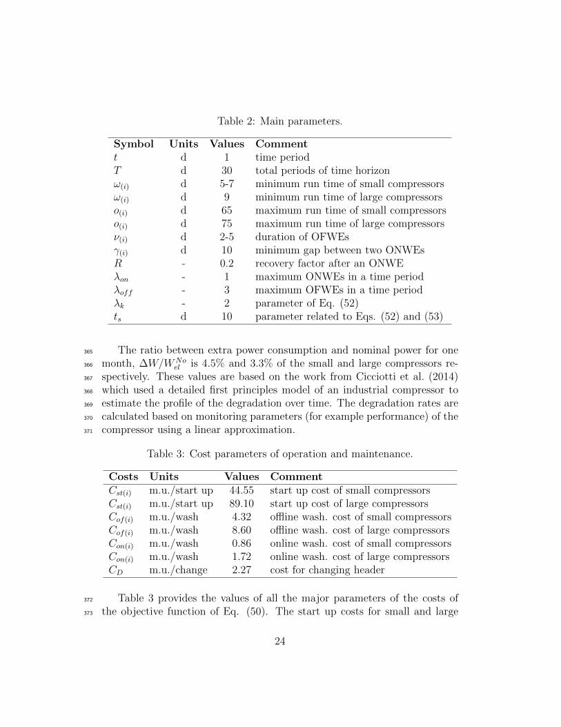
Table 2: Main parameters.
Symbol Units Values Commentt d 1 time periodT d 30 total periods of time horizonω(i) d 5-7 minimum run time of small compressorsω(i) d 9 minimum run time of large compressorso(i) d 65 maximum run time of small compressorso(i) d 75 maximum run time of large compressorsν(i) d 2-5 duration of OFWEsγ(i) d 10 minimum gap between two ONWEsR - 0.2 recovery factor after an ONWEλon - 1 maximum ONWEs in a time periodλoff - 3 maximum OFWEs in a time periodλk - 2 parameter of Eq. (52)ts d 10 parameter related to Eqs. (52) and (53)
The ratio between extra power consumption and nominal power for one365
month, ∆W/WNoel is 4.5% and 3.3% of the small and large compressors re-366
spectively. These values are based on the work from Cicciotti et al. (2014)367
which used a detailed first principles model of an industrial compressor to368
estimate the profile of the degradation over time. The degradation rates are369
calculated based on monitoring parameters (for example performance) of the370
compressor using a linear approximation.371
Table 3: Cost parameters of operation and maintenance.
Costs Units Values CommentCst(i) m.u./start up 44.55 start up cost of small compressorsCst(i) m.u./start up 89.10 start up cost of large compressorsCof(i) m.u./wash 4.32 offline wash. cost of small compressorsCof(i) m.u./wash 8.60 offline wash. cost of large compressorsCon(i) m.u./wash 0.86 online wash. cost of small compressorsCon(i) m.u./wash 1.72 online wash. cost of large compressorsCD m.u./change 2.27 cost for changing header
Table 3 provides the values of all the major parameters of the costs of372
the objective function of Eq. (50). The start up costs for small and large373
24

compressors were assumed equal to the energy consumed from the motors of374
the compressors for half a day. The current work assumed that there is not375
a major energy consumption for switching off a compressor, therefore this376
cost is zero. The washing costs are estimated using the assumptions from377
Aretakis et al. (2012) and Fabbri et al. (2011). Therefore, Table 3 gives the378
values of the costs of a washing episode in this particular case study of the379
compressors of BASF. The cost for changing header has been explained by380
Kopanos et al. (2015).381
Table 4: Initial state of the system.
Compressor i1 i2 i3 i4 i5 i6 i7 i8 i9 i10 i11Header - j1 - - j2 j2 - j1 - j3 j3ω(i) 0 6 0 0 40 22 0 20 0 40 55
ψ(i) 30 0 18 20 0 0 30 0 30 0 0δSo(i) 20 6 50 0 40 22 20 20 0 40 55
doof(i) 1 0 0 3 0 0 0 0 1 0 0
doon(i) - 2 - - - - - - - 1 5
A base case study is formulated to examine the optimal operation and382
maintenance plan of compressors with different types of washings. This base383
case uses the information from Tables 1, 2 and 3. Moreover, the information384
of the initial state of the system is provided by Table 4. The base case employs385
modified production targets for O2, N2 and compressed air for utilities from386
real industrial data. Figure 6 gives the production targets for O2 and N2 in387
kg of compressed air (scaled units).388
5. Results and discusions389
5.1. Base case study390
All given data and reported results are normalized and made dimension-391
less due to confidentiality reasons. All optimization problems have been392
solved in GAMS/CPLEX 11.1, under default configurations, in an Intel(R)393
Core(TM) i7-2600 CPU @3.4 GHz with 8 GB RAM. A zero optimality gap394
has been imposed in all problems instances.395
The base case study considers three different optimization problems with396
respect to each available washing method: only online washing (ON), only397
25

Dem
and
in k
g ai
r per
day
(sca
led)
N2
O2
Figure 6: Production targets of the air separation plant for thirty days.
Table 5: Problem specifications, and value of objective function in scaledmonetary units of each scenario.
Cases eqns bin vars cont vars nodes CPU (s) ObjON 14267 2640 4380 514 51 983OFF 14638 3297 4050 749 137 1022ON+OFF 16601 3627 4707 522 85 996
offline (OFF) and both washings (ON+OFF). The specifications of each op-398
timization problem and the values of the objective functions of each solution399
can be seen in Table 5.400
The number of variables of the OFF case is larger than the ON case and401
the number of variables in the ON+OFF case is considerably larger than in402
the OFF case due to the consideration of the extended mathematical model403
described in Section 3.3. Furthermore, Table 5 shows that the problem in the404
OFF case takes relatively more time than in the other two cases to be solved.405
The reason for this is that in the OFF case a compressor can be washed only406
if it is offline. Therefore, the offline washing cost is implicitly connected with407
the cost of a start up. Indeed, if a compressor which has been washed after408
a shut down has to to operate again, then it has to start up with a start up409
penalty. On the other hand in the ON case the online washing can prolong410
the operational time of the compressor without shutting it down.411
26
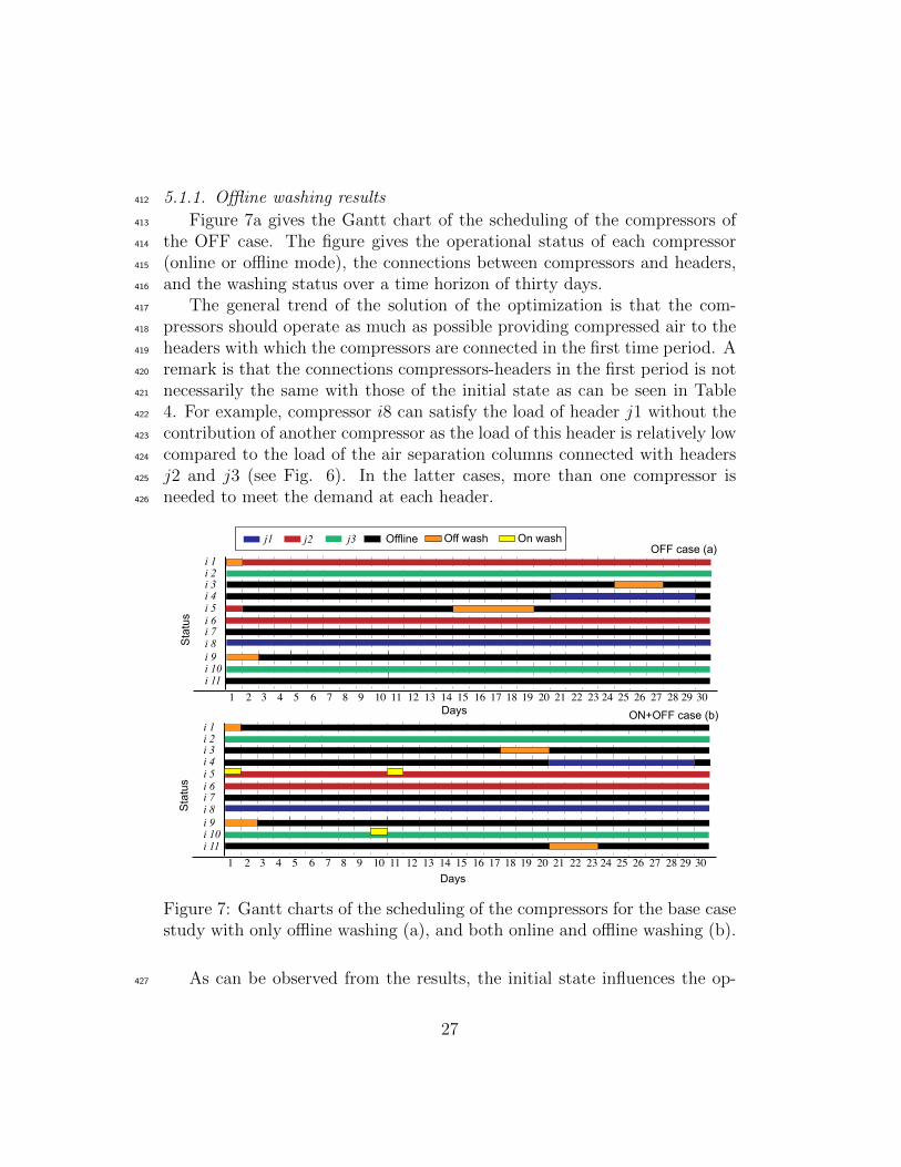
5.1.1. Offline washing results412
Figure 7a gives the Gantt chart of the scheduling of the compressors of413
the OFF case. The figure gives the operational status of each compressor414
(online or offline mode), the connections between compressors and headers,415
and the washing status over a time horizon of thirty days.416
The general trend of the solution of the optimization is that the com-417
pressors should operate as much as possible providing compressed air to the418
headers with which the compressors are connected in the first time period. A419
remark is that the connections compressors-headers in the first period is not420
necessarily the same with those of the initial state as can be seen in Table421
4. For example, compressor i8 can satisfy the load of header j1 without the422
contribution of another compressor as the load of this header is relatively low423
compared to the load of the air separation columns connected with headers424
j2 and j3 (see Fig. 6). In the latter cases, more than one compressor is425
needed to meet the demand at each header.426
1 2 3 4 5 6 7 8 9 10 11 12 13 14 15 16 17 18 19 20 21 22 23 24 25 26 27 28 29 30
i 1i 2
i 4
i 8
i 3
i 11
i 9i 10
j1 j2 j3 Off washOffline On wash
Sta
tus i 6
i 5
i 7
Days
OFF case (a)
ON+OFF case (b)
1 2 3 4 5 6 7 8 9 10 11 12 13 14 15 16 17 18 19 20 21 22 23 24 25 26 27 28 29 30
i 1i 2
i 4
i 8
i 3
i 11
i 9i 10
Days
Sta
tus i 6
i 5
i 7
Figure 7: Gantt charts of the scheduling of the compressors for the base casestudy with only offline washing (a), and both online and offline washing (b).
As can be observed from the results, the initial state influences the op-427
27
timal solution. For instance, Fig. 7a shows that in the beginning of the428
optimization compressor i11 is switched off and it is not used at all. In addi-429
tion, in the beginning of optimization compressor i2 has changed from header430
j1 to j3. The reason for this is that compressor i11 has higher minimum limit431
of mass flow rate than compressor i2, therefore compressor i11 switches off432
and compressor i2 satisfies the load of header j3 along with compressor i10.433
These changes support the further decisions which switch off compressor i5434
at day 2 and start up compressor i1 connecting to header j2.435
The optimization suggests maintaining compressors i3 and i5 which have436
been operated more than the others as can be seen from the values of δSo(i)437
in Table 4. Hence, this decision leads to lower maintenance costs compared438
to the scenario which could have decided the washing of a larger compressor439
such as compressor i11. Table 3 shows that the offline washing cost of a small440
compressor is lower than the cost of a large compressor. In the section of441
the time horizon between Day 15 and Day 30, the two washing episodes of442
compressors i3 and i5 are derived from the terminal constraints in Eqs. (52)443
and (53) with the consideration of λk = 2 and t∗S = 15 d.444
The previous statements show that there are many factors which influence445
the best decisions for optimal operation of the compressors and these factors446
depend on the knowledge of the future information such as forecast of the447
demand and the decisions for the succeeding time periods. Moreover, the448
values of the parameters of the problem influence these decisions. Examples449
of these parameters are the initial operating and shut down times, and the450
values of the penalty costs.451
Thus, even the most well trained and experienced team of managers and452
operators could find it difficult to take the best decisions without having a453
sophisticated optimization model based on the systematic use of the previous454
mentioned information. The nature of the problem is combinatorial involving455
a large number of scenarios, and therefore it is impractical and probably456
impossible to identify the optimal patterns for the best decisions without the457
use of optimization.458
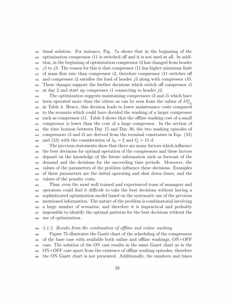
5.1.2. Results from the combination of offline and online washing459
Figure 7b illustrates the Gantt chart of the scheduling of the compressors460
of the base case with available both online and offline washings, ON+OFF461
case. The solution of the ON case results in the same Gantt chart as in the462
ON+OFF case apart from the existence of offline washing episodes, therefore463
the ON Gantt chart is not presented. Additionally, the numbers and times464
28

Days
i1
i8
i2
i6
i10
i5
ΔWel
(i,t)(
%)
Shut down (i5) Start up (i4)
i4
(a) OFF base case
i6
i5
i8i2
i4
i10
ΔWel
(i,t)(
%)
Start up
online wash
(b) ON+OFF base case
Figure 8: Extra power consumption (scaled) over time.
of the online washing episodes (ONWEs) are the same in both cases.465
The results from the schedule of the ON+OFF case show that online466
washing is used along with offline. In this case compared to the OFF case,467
compressor i5 is not switched off but it is washed online. Hence, both sched-468
ules included cleaning of compressor i5, the OFF case with offline washing,469
but the ON+OFF with online and keeping the compressor on. The reason470
is that this small compressor is the second most fouled one after compressor471
i11. As the schedule of the OFF case switched off compressor i11 the same472
can be observed in the schedule of the ON+OFF case. In the latter case,473
compressor i5 remains online and therefore only compressors i7 and i11 can474
be washed offline. The other smaller compressors cannot be washed offline475
as i1, i4 have been washed before the beginning of the optimization and the476
other compressors i2, i5 remain online over the whole time horizon.477
Figure 8 illustrates the extra power consumption ∆Wel(i,t) of each com-478
pressor i in scaled units, this means that if the real extra power is ∆W ∗el(i,t)479
in kW and a fixed parameter ∆W s(i) is given in kW, then the vertical axis480
shows the scaled variable ∆Wel(i,t) = ∆W ∗el(i,t)/∆W
s(i) with no units.481
The ON case results in minimum total cost compared to the other two482
cases as can be seen in Fig. 9a. However, the ON case does not include483
terminal constraints as cases OFF and ON+OFF considering them. At the484
end of the optimization the total Equivalent Operating Time (EOT) in days485
of the compressors are 405, 321 and 280 in ON, OFF and ON+OFF cases486
respectively. Therefore, the ON+OFF case achieves 2.5% lower total cost487
29

ON OFF ON+OFFC
ost u
nits
Total Wel Welc
ONOFFON+OFF
Cos
t uni
ts
ΔWelWashing offline
Washingonline
Changeheader
Start up
Figure 9: Total and electricity costs (a) and other costs (b) for thirty days.
than the one in the OFF case and the compressors have been operated 41488
days less. Therefore, the former case achieved to meet the demand with489
decreased operational costs and to wear less the compressors due to less490
equivalent operating time compared to the latter case.491
Figure 9b explains that in the case of ON+OFF the total cost is lower,492
even if the costs of the washings are higher, than in the case of OFF. However,493
the total electricity Wel consumed in the ON+OFF is higher than in the494
case of the OFF. This proves that the maintenance strategy considerably495
influences the operation. The main reason that the schedule in the ON+OFF496
case is less expensive than the OFF is that the online washing complements to497
the offline, thus this results in fewer start up events. The results which show498
that a compressor has to operate online continuously as much as possible is499
mostly in line with the industrial policy. This is justified as Fig. 7a shows500
that compressor i5 shuts down after 41 days and Fig. 7b shows that the same501
compressor operates for 70 days equal to 53.2 equivalent operating days.502
5.2. Different degradation rates503
5.2.1. Description of case studies504
Section 5.2 examines the influence of different degradation rates on the505
scheduling of the compressors. In the base case study the degradation rate506
is based on 4.5% and 3.3% extra power consumption per month of the small507
and the large compressors respectively in the air separation plant in BASF,508
Ludwigshafen, Germany. These degradation rates define the low degradation509
rate case (Low case). A Medium and a High case consider 6% and 9% extra510
power consumption per month for small and large compressors. Aretakis et511
30
al. (2012) stated that 10% extra power consumption per month is relatively512
significant but it can also be realistic.513
The structure of the network of compressors and headers, the air separa-514
tion columns, storage tanks and customers are the same as in those of the515
base case. Moreover, the input from the Tables 1, 2, 3 and 4 remain the516
same.517
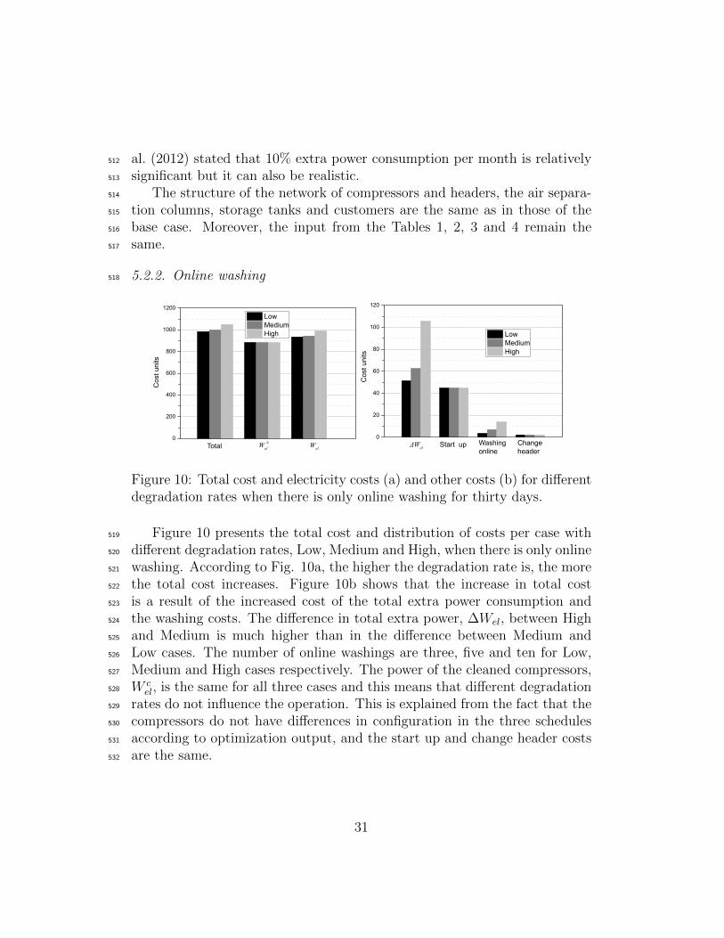
5.2.2. Online washing518
Cos
t uni
ts
Total Wel Welc
LowMediumHigh
Cos
t uni
ts
ΔWelWashingonline
Changeheader
Start up
LowMediumHigh
Figure 10: Total cost and electricity costs (a) and other costs (b) for differentdegradation rates when there is only online washing for thirty days.
Figure 10 presents the total cost and distribution of costs per case with519
different degradation rates, Low, Medium and High, when there is only online520
washing. According to Fig. 10a, the higher the degradation rate is, the more521
the total cost increases. Figure 10b shows that the increase in total cost522
is a result of the increased cost of the total extra power consumption and523
the washing costs. The difference in total extra power, ∆Wel, between High524
and Medium is much higher than in the difference between Medium and525
Low cases. The number of online washings are three, five and ten for Low,526
Medium and High cases respectively. The power of the cleaned compressors,527
W cel, is the same for all three cases and this means that different degradation528
rates do not influence the operation. This is explained from the fact that the529
compressors do not have differences in configuration in the three schedules530
according to optimization output, and the start up and change header costs531
are the same.532
31

5.2.3. Offline washing533
Figure 11 illustrates the total cost, electricity cost distribution and other534
costs when only offline washing is available. The decisions of operation and535
maintenance of the Medium and High cases are the same with those of the536
base case. For this reason the W cel and offline washing costs are the same537
for all three cases. The difference in total extra power between medium and538
low degradation rate is 31.3% and the difference between high and medium539
is 91.6%. This results in higher total cost in the High case. Moreover, the540
optimization suggests keeping the online compressors operating as much as541
possible to avoid start up costs or possible change header costs.542
Cos
t uni
ts
Total Wel Welc
LowMediumHigh
Cos
t uni
ts
ΔWelWashingoffline
Changeheader
Start up
LowMediumHigh
Figure 11: Total cost and electricity costs (a) and other costs (b) for differentdegradation rates when there is only offline washing for thirty days.
5.2.4. Both online and offline washing543
Figure 12 shows that the combination of online and offline washings544
achieve reduced total costs by 2.5%, 2.5% and 3.0% in each degradation545
rate case respectively compared to the OFF case presented in Section 5.2.3.546
However, only in the High case the extra power ∆Wel cost is lower in the547
case of the ON+OFF case than in the OFF case. The total cost of the548
OFF case includes increased start up costs, on the other hand the ON+OFF549
case is more flexible with lower total start up cost. The previous observa-550
tions support the use of both online and offline washing, especially when the551
Equivalent Operating Time (EOT) of the ON+OFF case is reduced by 35%552
compared to this of the OFF case. This shows that the operation of com-553
pressors in the former case would be more flexible for a following scheduling554
problem as the compressors have been maintained in a more optimal way in555
the current scheduling problem.556
32
LowMediumHigh
Cos
t uni
ts
Total Wel Welc
Cos
t uni
ts
ΔWelWashingoffline
Washingonline
Changeheader
Start up
LowMediumHigh
Figure 12: Total cost and electricity costs (a) and other costs (b) for differentdegradation rates when both offline and online washing are considered forthirty days.
1 2 3 4 5 6 7 8 9 10 11 12 13 14 15 16 17 18 19 20 21 22 23 24 25 26 27 28 29 30
i 1i 2
i 4
i 8
i 3
i 11
i 9i 10
Days
Sta
tus
i 6i 5
i 7
j1 j2 j3 Off washOffline On wash
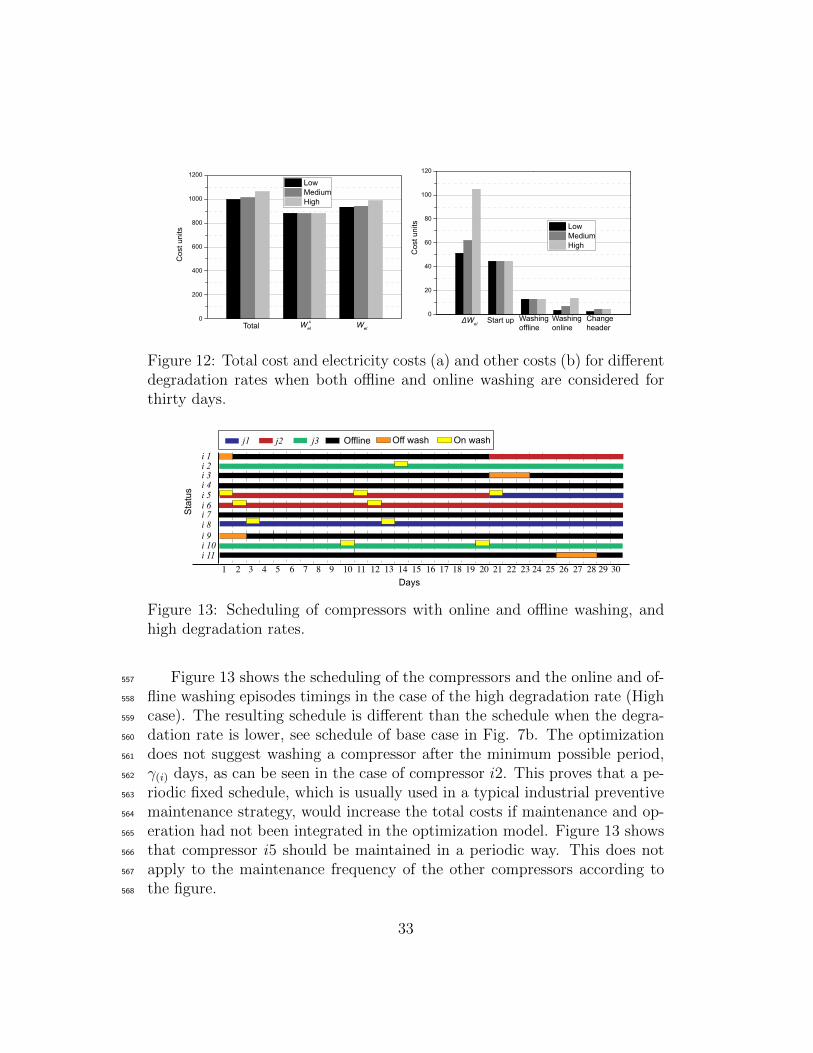
Figure 13: Scheduling of compressors with online and offline washing, andhigh degradation rates.
Figure 13 shows the scheduling of the compressors and the online and of-557
fline washing episodes timings in the case of the high degradation rate (High558
case). The resulting schedule is different than the schedule when the degra-559
dation rate is lower, see schedule of base case in Fig. 7b. The optimization560
does not suggest washing a compressor after the minimum possible period,561
γ(i) days, as can be seen in the case of compressor i2. This proves that a pe-562
riodic fixed schedule, which is usually used in a typical industrial preventive563
maintenance strategy, would increase the total costs if maintenance and op-564
eration had not been integrated in the optimization model. Figure 13 shows565
that compressor i5 should be maintained in a periodic way. This does not566
apply to the maintenance frequency of the other compressors according to567
the figure.568
33
i2
i1
i5
i6i8
i10
ΔWel
(i,t)(
%)
online wash
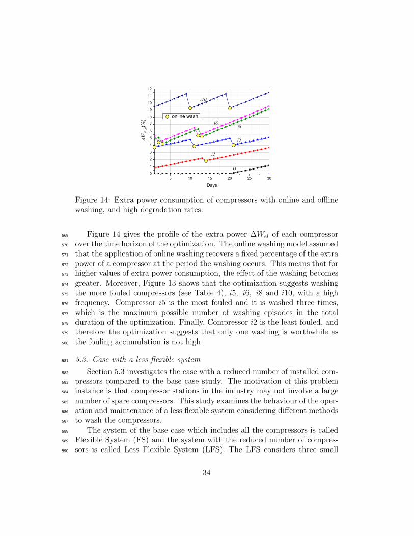
Figure 14: Extra power consumption of compressors with online and offlinewashing, and high degradation rates.
Figure 14 gives the profile of the extra power ∆Wel of each compressor569
over the time horizon of the optimization. The online washing model assumed570
that the application of online washing recovers a fixed percentage of the extra571
power of a compressor at the period the washing occurs. This means that for572
higher values of extra power consumption, the effect of the washing becomes573
greater. Moreover, Figure 13 shows that the optimization suggests washing574
the more fouled compressors (see Table 4), i5, i6, i8 and i10, with a high575
frequency. Compressor i5 is the most fouled and it is washed three times,576
which is the maximum possible number of washing episodes in the total577
duration of the optimization. Finally, Compressor i2 is the least fouled, and578
therefore the optimization suggests that only one washing is worthwhile as579
the fouling accumulation is not high.580
5.3. Case with a less flexible system581
Section 5.3 investigates the case with a reduced number of installed com-582
pressors compared to the base case study. The motivation of this problem583
instance is that compressor stations in the industry may not involve a large584
number of spare compressors. This study examines the behaviour of the oper-585
ation and maintenance of a less flexible system considering different methods586
to wash the compressors.587
The system of the base case which includes all the compressors is called588
Flexible System (FS) and the system with the reduced number of compres-589
sors is called Less Flexible System (LFS). The LFS considers three small590
34

Cost units
LFS ON+OFF
FS ON+OFF
LFS OFF
FS OFF
LFS ON
FS ONLow Medium High
Figure 15: Comparison of total costs between a Flexible System (FS) and aLess Flexible System (LFS)
compressors i ∈ Is = i2, i4, i5 and four large compressors i ∈ Il =591
i6, i8, i10, i11.592
Figure 15 shows the results from the Less Flexible System (LFS) and593
Flexible System (FS) study for each washing method used, i.e. ON, OFF594
and ON+OFF, and for each degradation rate case, i.e. Low, Medium and595
High. The results illustrate that the less flexible system is associated with596
higher total costs in all cases compared to the Flexible system, apart from597
the cases with the only available online washing (case ON). Indeed, the costs598
of both systems in the ON case are exactly the same.599
The less flexible system has higher total cost in the OFF scenario and in600
all degradation rate cases by 0.8% and increased total cost in the ON+OFF601
case by approximately 3%. There is no difference in the ON case. This602
explains that the online washing along with the offline and with the use of603
spare compressors (i.e. flexible system) improves significantly the operation604
compared to the less flexible system case. This remark is important as com-605
pressors eventually must be washed offline at some point.606
The impact of the flexibility of a system of compressors, which is associ-607
ated with the increased number of spare compressors, on the total cost can608
be seen in the case of the Flexible System (FS) where the ON+OFF washing609
reduces the total cost compared to the OFF washing case. However, this610
reduction is less important in the case of the Less Flexible System (LFS).611
The capital costs in the case of a compressor station with a reduced num-612
35
ber of parallel units are lower compared a compressor station with a number613
of spare units. According to literature (Xenos et al., 2015b; Saidur et al.,614
2010), the capital cost of a compressor is significantly lower than the oper-615
ational and maintenance costs in its lifecycle which is usually more than 30616
years. Therefore, a framework to determine optimal operation and mainte-617
nance of an existing installation of compressors is necessary to reduce opera-618
tional costs independently if the selection of the number of the compressors619
and the decision of the proper sizing of the compressors was successful at the620
front end design of the plant. A sophisticated approach which examines the621
simultaneous optimal selection of the installed compressors and their sizing,622
and the operational planning of the plant can be a future topic of research.623
6. Conclusions624
This paper presented an integrated optimization framework which can be625
used to optimize operation and maintenance of multiple compressors with626
different types of washings, namely offline and online. The optimization627
framework determines when and how often to wash the compressors using628
each washing method. The results showed that the best maintenance strat-629
egy to decrease the total costs and at the same time to minimize the wear of630
the compressors is a combination of offline and online washing. In the case631
which a compressor network involves spare compressors, the use of both wash-632
ings decreases the total costs and increases the availability of the compressor633
significantly. The results have shown that the optimization framework can634
provide enhanced decision support leading to optimal operation and mainte-635
nance. By the modification of the constraints (i.e. compressor and models of636
the units of the plant), the optimization framework can be applied to other637
systems which include parallel compressors with large power consumption.638
7. Acknowledgments639
Financial support from the Marie Curie FP7-ITN project “Energy sav-640
ings from smart operation of electrical, process and mechanical equiment -641
ENERGY SMARTOPS”, Contract No: PITN-GA-2010-264940 is gratefully642
acknowledged. The authors would like to thank BASF SE for providing a643
case study and technical support.644
36

References645
Aretakis N., Roumeliotis I., Doumouras G., Mathioudakis K., 2012, Com-646
pressor washing economic analysis and optimization for power generation,647
Applied Energy, 95, pp. 77–86.648
de Backer W., 2000, Modular uprating and upgrading solution in ABB Al-649
stom power gas turbines, ASME, 2000-GT-306.650
Biondi M., Sand G., Harjunkoski I., 2015, Tighter integration of maintenance651
and production in short-term scheduling of multipurpose process plants,652
12th International Symposium on Process Systems Engineering and 25th653
European Symposium on Computer Aided Process Engineering, 31 May–4654
June, Copenhagen, Denmark.655
Bohrenkamper G., Bals H., Wrede U., Umlauf R., 2000, Hot-gas-path life656
extension options for the V94.2 gas turbine, ASME, 2000-GT-178.657
Boyce M.P., 2003, Centrifugal Compressors: A Basic Guide, PennWell Cor-658
poration, Oklahoma, USA.659
Boyce M. P., Gonzalez F., 2007, A study of on-line and off-line turbine wash-660
ing to optimize the operation of a gas turbine, Journal of Engineering for661
Gas Turbines and Power, Transactions of the ASME, 129, pp. 114–122.662
Camponogara E., Nazari L.F., Meneses C.N., 2012, A revised model for663
compressor design and scheduling in gas-lifted oil fields, IIE Transactions,664
44 (5), pp. 342–351.665
Castro P.M., Grossmann I.E., Veldhuizen P, Esplin D., 2014, Optimal main-666
tenance scheduling of a gas engine power plant using generalized disjunc-667
tive programming, AIChE, 60 (6), 2083 – 2097.668
Cicciotti M., Xenos D.P., Bouaswaig A.E.F., Thornhill N.F., Martinez-Botas669
R., 2014, Online performance monitoring of industrial compressors using670
meanline modelling, Proceedings of ASME Turbo Expo 2014, June 16–20,671
Dusseldorf, Germany, GT2014-25088.672
Cobos-Zaleta D., Rıos-Mercado R.Z., 2002, A MINLP model for minimizing673
fuel consumption on natural gas pipeline networks, Memorias del XI Con-674
greso Latino Iberoamericano de Investigacion de Operaciones (CLAIO),675
27–31 October, Chile.676
37

Diakunchak I.S., 1992, Performance deterioration in industrial gas turbines,677
Journal of Engineering for Gas Turbines and Power, 114 (2), pp. 161–168.678
Fabbri A., Traverso A. and Cafaro S., 2011, Compressor performance re-679
cover system: which solution and when, Proceedings of the Institution of680
Mechanical Engineers, Part A: Journal of Power and Energy, pp. 457–466.681
Forsthoffer W. E., 2011, Forsthoffer’s Best Practice Handbook for Rotating682
Machinery, Butterworth-Heinemann, Boston, USA.683
Gopalakrishnan A., Biegler L.T., 2013, Economic nonlinear model predictive684
control for periodic optimal operation of gas pipeline networks, Computers685
and Chemical Engineering, 52, pp. 90–99.686
Gustavsson E., Patriksson M., Stromberg A.-B., Wojciechowski A., Onnheim687
M., 2014, Preventive maintenance scheduling of multi-component systems688
with interval costs, Computers and Industrial Engineering, 76, pp. 390–689
400.690
Han I.-S, Han C., Chung C.-B., 2004. Optimization of the air-and gas-supply691
network of a chemical plant, Chemical Engineering Research and Design,692
82 (A10), pp. 1337–1343.693
Hasan M.M.F., Razib Md.S., Karimi I.A., 2009, Optimization of compressor694
networks in LNG operations, 10th International Symposium on Process695
Systems Engineering - PSE2009, pp. 1767–1772.696
Hazaras M.J., Swartz C.L.E, Marlin T.E., 2012, Flexible maintenance within697
a continuous-time state-task network framework, Computers and Chemical698
Engineering, 46, pp. 167–177.699
van den Heever S.A., Grossmann I.E., 2003, A strategy for the integration700
of production planning and reactive scheduling in the optimization of a701
hydrogen supply network, Computers and Chemical Engineering, 27 (12),702
pp. 1813–1839.703
Kopanos G.M., Pistikopoulos E.N., 2014, Reactive scheduling by a multi-704
parametric programming rolling horizon framework: A case of a network705
of combined heat and power units, Industrial and Engineering Chemistry706
Research, 53 (11), pp. 4366–4386.707
38

Kopanos G. M., Xenos D.P., Cicciotti M., Pistikopoulos E.N., Thonrhill N.F,708
2015, Optimization of a network of compressors in parallel: Operational709
and maintenance planning - The air separation plant case, Applied Energy,710
146, pp. 453–470.711
Kurz R., Lubomirsky M., Brun K., 2012, Gas compressor station economic712
optimization, International Journal of Rotating Machinery, 12, pp. 1–9.713
Li Y.G., Nilkitsaranont P., 2009, Gas turbine performance prognostic for714
condition-based maintenance, Applied Energy, 86, pp. 2152–2161.715
Liu S., Yahia A., Papageorgiou L.G., 2014, Optimal production and main-716
tenance planning of biopharmaceutical manufacturing under performance717
decay, Industrial and Engineering Chemistry Research, 53 (44), pp. 17075-718
17091.719
Luo, X., Zhang B., Chen Y., Mo S., 2013, Operational planning optimiza-720
tion of steam power plants considering equipment failure in petrochemical721
complex, Applied Energy, 11, pp. 1247–1264.722
Marcovecchio M.G., Novais A.Q., Grossmann I.E., 2014, Deterministic opti-723
mization of the thermal Unit Commitment problem: A Branch and Cut724
search, Computers and Chemical Engineering, 67, pp. 53–68.725
Meher-Homji C.B., Chaker M., Motiwalla H., 2001, Gas turbine performance726
deterioration, Proceedings of the 30th Turbomachinery Symposium, Hous-727
ton, Texas, September 17–20.728
Saidur R., Rahim, N.A., Hasanuzzaman, M., 2010, A review on compressed-729
air energy use and energy savings, Renewable and Sustainable Energy Re-730
views, 14 (4), pp. 1135–1153.731
Sanchez D., Chacartegui R., Becerra J.A., Sanchez, T., 2009, Determining732
compressor wash programmes for fouled gas turbines, Journal of Power733
and Energy, Proceedings IMechE, 223 Part A, pp. 467–476.734
Sequeira S.E., Graells M., Puigjaner L., 2001, Decision-making framework735
for the scheduling of cleaning/maintenance tasks in continuous parallel736
lines with time-decreasing performance, European Symposium on Com-737
puter Aided Process Engineering - 11, Computer Aided Chemical Engi-738
neering, 9, pp. 913–918.739
39

Sun H., Ding H., 2014, Plant simulation and operation optimization of SMR740
plant with different adjustment methods under part-load conditions, Com-741
puters and Chemical Engineering, 68, pp. 107–113.742
Vecchietti A., Sangbum L., Grossmann I.E, 2003, Modeling of dis-743
crete/continuous optimization problems: characterization and formulation744
of disjunctions and their relaxations, Computers and Chemical Engineer-745
ing, 27, pp. 433–448.746
Xenos D.P., Kopanos G.M., Cicciiotti M., Pistikopoulos E.N., Thornhill747
N.F., 2014, Operational optimization of compressors in parallel considering748
condition-based maintenance, European Symposium on Computer Aided749
Process Engineering (ESCAPE 24), June 15–18, Budapest, Hungary.750
Xenos D.P., Cicciotti M., Kopanos M.G., Bouaswaig A.E.F, Kahrs O.,751
Martinez-Botas R., Thornhill N.F., 2015a, Optimization of a network of752
compressors in parallel: Real Time Opimization (RTO) of compressors753
in chemical plants – An industrial case study, Applied Energy, 144, pp.754
51–63.755
Xenos D.P., Lunde E., Thornhill N.F., 2015b, Optimal operation and main-756
tenance of gas compressor stations: An integrated framework applied to757
a large-scale industrial case, Proceedings of ASME Turbo Expo 2015, June758
15–19, Montreal, Canada, GT2015–44002.759
Zavala V.M., 2014, Stohastic optimal control model for natural gas networks,760
Computers and Chemical Engineering, 64, pp. 103–113.761
40

Appendix762
The basic operational model of networks of compressors connected with763
different headers and downstream processes can be seen in Tables 6, 7 and764
8. The logical constraints (54) – (56) connect the binary variables of start765
up S(i,t) and shut down F(i,t) with the binary variable which defines the766
status of the compressor X(i,t). The parameter χ(i) is the initial status of the767
compressors exactly before the beginning of the optimization. Constraints768
(54) – (56) are related to constraints (57) and (58) which define the minimum769
start up and shut down times of the compressors.770
Table 6: Operational model and basic constraints (Kopanos et al., 2015).
Logical constraints of start up and shut down decisions:
S(i,t) − F(i,t) = X(i,t) − χ(i), ∀i ∈ I, t = 1 (54)
S(i,t) − F(i,t) = X(i,t) −X(i,t−1), ∀i ∈ I, t > 1 (55)
S(i,t) + F(i,t) ≤ 1, ∀i ∈ I, t ∈ T (56)
Minimum start up/shut down times:
X(i,t) ≥t∑
t′=max1,t−ω(i)+1
S(i,t′), ∀i ∈ I, t ∈ T : ω(i) > 1 (57)
1−X(i,t) ≥t∑
t′=max1,t−ψ(i)+1
F(i,t′), ∀i ∈ I, t ∈ T : ψ(i) > 1 (58)
Equations (59) and (60) in Table 7 define the feasible window of operation771
of compressor i ∈ I. The expression of the power consumption is valid within772
these operational bounds defined by the two equations. The parameters ρ(i)773
and π(i) define the minimum and maximum boundaries of the decision vari-774
ables mass flow and outlet pressure of the compressors. The logical constraint775
(61) restrict online compressors to provide compressed air to more than one776
header. The constraints (62) – (63) model the change D(i,t) of a compressor777
to different headers. The parameter φ(i,j) denotes the initial connections of778
the compressors i ∈ I with headers j ∈ J(i) exactly before the beginning of779
the optimization. The relation between outlet pressure of a compressor P(i,j,t)780
41

Table 7: Operational model and basic constraints (Kopanos et al., 2015).
Operating bounds of the compressors:
ρmin(i) Y(i,j,t) ≤M(i,j,t) ≤ ρmax(i) Y(i,j,t), ∀i ∈ I, j ∈ J(i), t ∈ T (59)
πmin(i) Y(i,j,t) ≤ P(i,j,t) ≤ πmax(i) Y(i,j,t), ∀i ∈ I, j ∈ J(i), t ∈ T (60)
Logical constraints and discharge pressure at the grids:∑j∈J(i)
Y(i,j,t) = X(i,j,t), ∀i ∈ I, t ∈ T (61)
D(i,t) ≥ Y(i,j,t) − φ(i,j) − S(i,t), ∀i ∈ I, j ∈ J(i), t = 1 (62)
D(i,t) ≥ Y(i,j,t) − Y(i,j,t−1) − S(i,t), ∀i ∈ I, j ∈ J(i), t > 1 (63)
P(i,j,t) = a(j)M(i,j,t) + b(j)Y(i,j,t)∀i ∈ I, j ∈ J(i), t ∈ T (64)
and total mass flow in the header M(i,j,t) is described by Eq. (64). This is781
a linear relation with parameters a(j) and b(j) estimated by fitting industrial782
data.783
Table 8 gives the mass balances and operational boundaries of the air784
separation columns u ∈ U and storage tanks z ∈ Z. The network of com-785
pressors has to satisfy the compressed air for utilities with demand θ(n,t) for786
every process plant n ∈ N and this is given by Eq. (65). Equations. (66) –787
(68) describe the mass balance and capacity boundaries of the air separation788
columns. The outlet mass flow of product e is given from Eq. (66) where789
the parameter σ(e) is the volumetric fraction of the primary component of790
air e. The variable L(e,u,z,t) is the total mass amount of product e provided791
to each storage tank z. Equations (69) – (72) give the mass balances in the792
storage tanks and for the end-users with demand ζ(e,t). The variable A(e,z,t)793
represents the amount of product e delivered to storage tank z, the variable794
B(e,z,t) is the amount of stored product e of storage tank z per period t, and795
the variable O(e,t) is the amount of product e purchased from external sources796
per period t. Parameters c(e,u) and ξ(e,z) are the boundaries of air separation797
columns and storage tanks. Finally, parameter β(e,z) is the initial inventory798
of product e of tank z before optimization.799
42

Table 8: Mass balances, and capacity and storage boundaries (Kopanos etal., 2015).
Demand of compressed air:∑i∈I
∑(j∈Jn∩J(i))
M(i,j,t) ≥ θ(n,t) ∀n ∈ N, t ∈ T (65)
Air separation columns operation:
C(e,u,t) = σ(e)∑i∈I
∑(j∈J(u)∩J(i))
M(i,j,t) ∀u ∈ U, t ∈ T (66)
∑z∈Z(e)
L(e,u,z,t) = ktC(e,u,t) ∀e ∈ E, u ∈ U, t ∈ T (67)
cmin(e,u) ≤ C(e,u,t) ≤ cmax(e,u) ∀e ∈ E, u ∈ U, t ∈ T (68)
Storage tanks and end-customers (demand side) mass balances, ∀e ∈ E:∑z∈Z(e)
A(e,z,t) +O(e,t) = ζ(e,t), ∀t ∈ T (69)
B(e,z,t) = β(e,z) +∑u∈Uz
L(e,u,z,t) − A(e,z,t), ∀z ∈ Z(e), t = 1 (70)
B(e,z,t) = B(e,z,t−1) +∑u∈Uz
L(e,u,z,t) − A(e,z,t), ∀z ∈ Z(e), t > 1 (71)
ξmin(e,z) ≤ B(e,z,t) ≤ ξmax(e,z), ∀z ∈ Z(e), t ∈ T (72)
43