Cleveland State University Cleveland State University

EngagedScholarship@CSU EngagedScholarship@CSU

ETD Archive

2015

Optimal Design and Control of a Lower-Limb Prosthesis with Optimal Design and Control of a Lower-Limb Prosthesis with

Energy Regeneration Energy Regeneration

Holly E. Warner Cleveland State University

Follow this and additional works at: https://engagedscholarship.csuohio.edu/etdarchive

Part of the Mechanical Engineering Commons

How does access to this work benefit you? Let us know! How does access to this work benefit you? Let us know!

Recommended Citation Recommended Citation Warner, Holly E., "Optimal Design and Control of a Lower-Limb Prosthesis with Energy Regeneration" (2015). ETD Archive. 679. https://engagedscholarship.csuohio.edu/etdarchive/679

This Thesis is brought to you for free and open access by EngagedScholarship@CSU. It has been accepted for inclusion in ETD Archive by an authorized administrator of EngagedScholarship@CSU. For more information, please contact library.es@csuohio.edu.

OPTIMAL DESIGN AND CONTROL

OF A LOWER-LIMB PROSTHESIS

WITH ENERGY REGENERATION

HOLLY E. WARNER

Bachelor of Science in Mechanical Engineering

Cleveland State University

May 2014

submitted in partial fulfillment of requirements for the degree

MASTERS OF SCIENCE IN MECHANICAL ENGINEERING

at the

CLEVELAND STATE UNIVERSITY

AUGUST 2015

We hereby approve this thesis for

HOLLY E. WARNER

Candidate for the Master of Science in Mechanical Engineering degree for the

Department of Mechanical Engineering

and the CLEVELAND STATE UNIVERSITY

College of Graduate Studies

Thesis Chairperson, Daniel Simon, Ph.D.

Department & Date

Thesis Committee Member, Hanz Richter, Ph.D.

Department & Date

Thesis Committee Member, Antonie van den Bogert, Ph.D.

Department & Date

Student’s Date of Defense: August 11, 2015

ACKNOWLEDGMENTS

My deepest gratitude goes to Dr. Simon, my advisor, for taking me on as

an undergraduate and opening my eyes to the world of research. Thank you also to

Dr. Richter for helping me develop a multidisciplinary perspective and his invaluable

instruction in the methods of bond graphs and simulation. I so appreciate Dr. van

den Bogert’s willingness to hold countless discussions on modeling the human system.

For the support of, clarifying discussions with, and inspiration of my labmates, I am

grateful. This work was supported by the Wright Center for Sensor Systems Engi-

neering and National Science Foundation grant 0826124. My family has graciously

offered their encouragement, patience, and all-around support throughout this pro-

cess, making it possible. I appreciate all you have given. And, above all, I thank

God, without whose order in the world the study of science would be impossible. To

Him alone be the glory!

OPTIMAL DESIGN AND CONTROL OF A LOWER-LIMB PROSTHESIS WITH

ENERGY REGENERATION

HOLLY E. WARNER

ABSTRACT

The majority of amputations are of the lower limbs. This correlates to a par-

ticular need for lower-limb prostheses. Many common prosthesis designs are passive

in nature, making them inefficient compared to the natural body. Recently as tech-

nology has progressed, interest in powered prostheses has expanded, seeking improved

kinematics and kinetics for amputees. The current state of this art is described in

this thesis, noting that most powered prosthesis designs do not consider integrating

the knee and the ankle or energy exchange between these two joints. An energy

regenerative, motorized prosthesis is proposed here to address this gap.

After preliminary data processing is discussed, three steps toward the realiza-

tion of such a system are completed. First, the design, optimization, and evaluation

of a knee joint actuator are presented. The final result is found to be consistently

capable of energy regeneration across a single stride simulation. Secondly, because of

the need for a prosthesis simulation structure mimicking the human system, a novel

ground contact model in two dimensions is proposed. The contact model is validated

against human reference data. Lastly, within simulation a control method combining

two previously published prosthesis controllers is designed, optimized, and evaluated.

Accurate tracking across all joints and ground reaction forces are generated, and

the knee joint is shown to have human-like energy absorption characteristics. The

successful completion of these three steps contributes toward the realization of an

optimal combined knee-ankle prosthesis with energy regeneration.

iv

TABLE OF CONTENTS

ABSTRACT iv

LIST OF FIGURES viii

LIST OF TABLES xi

I INTRODUCTION 1

1.1 Motivation . . . . . . . . . . . . . . . . . . . . . . . . . . . . . . 1

1.2 Literature Review . . . . . . . . . . . . . . . . . . . . . . . . . . 4

1.3 Thesis Contributions and Organization . . . . . . . . . . . . . . 5

II REFERENCE DATA 7

2.1 Cleveland Clinic Data Processing . . . . . . . . . . . . . . . . . . 8

2.2 Veterans Administration Data Processing . . . . . . . . . . . . . 10

2.2.1 Subject Dimensions . . . . . . . . . . . . . . . . . . . . 10

2.2.2 Position Data by Inverse Kinematics . . . . . . . . . . 12

2.2.3 Coordinate System Alignment . . . . . . . . . . . . . . 15

2.2.4 Velocity and Acceleration Data and Resampling . . . . 16

2.2.5 Foot Kinematic Model . . . . . . . . . . . . . . . . . . 17

2.3 Discussion . . . . . . . . . . . . . . . . . . . . . . . . . . . . . . 18

III ACTUATOR SYSTEM DESIGN AND OPTIMIZATION 19

3.1 Actuator Modeling . . . . . . . . . . . . . . . . . . . . . . . . . . 20

3.1.1 Geometry and Kinematics . . . . . . . . . . . . . . . . 21

3.1.2 Dynamic Models . . . . . . . . . . . . . . . . . . . . . 23

3.2 Open-Loop Control . . . . . . . . . . . . . . . . . . . . . . . . . 31

3.3 Simulation, Optimization, and Results . . . . . . . . . . . . . . . 32

v

3.3.1 Basic Actuator . . . . . . . . . . . . . . . . . . . . . . 32

3.3.2 Complex Friction Actuator . . . . . . . . . . . . . . . . 40

3.3.3 Generalized Friction Actuator . . . . . . . . . . . . . . 47

3.4 Discussion . . . . . . . . . . . . . . . . . . . . . . . . . . . . . . 54

IV GROUND CONTACT MODEL DESIGN AND OPTIMIZATION 56

4.1 Ground Contact Model . . . . . . . . . . . . . . . . . . . . . . . 57

4.1.1 Initial Hip Robot Contact Model . . . . . . . . . . . . 57

4.1.2 Novel Ground Contact Model . . . . . . . . . . . . . . 59

4.2 Contact Model Optimization . . . . . . . . . . . . . . . . . . . . 64

4.2.1 Particle Swarm Optimization . . . . . . . . . . . . . . 64

4.2.2 Contact Model Optimization . . . . . . . . . . . . . . . 66

4.3 Results . . . . . . . . . . . . . . . . . . . . . . . . . . . . . . . . 67

4.4 Discussion . . . . . . . . . . . . . . . . . . . . . . . . . . . . . . 73

V CONTROL SYSTEM DESIGN AND OPTIMIZATION 75

5.1 Hip Robot and Prosthesis Dynamic Model . . . . . . . . . . . . . 76

5.2 Robust Tracking/Impedance Control Overview . . . . . . . . . . 77

5.3 State-Based Gain Switching . . . . . . . . . . . . . . . . . . . . . 81

5.4 Switched Robust Tracking/Impedance Controller . . . . . . . . . 82

5.5 Controller Optimization . . . . . . . . . . . . . . . . . . . . . . . 84

5.6 Results . . . . . . . . . . . . . . . . . . . . . . . . . . . . . . . . 87

5.7 Discussion . . . . . . . . . . . . . . . . . . . . . . . . . . . . . . 92

VI CONCLUSIONS AND FUTURE WORK 94

BIBLIOGRAPHY 98

APPENDICES 105

A. Bond Graph Theory . . . . . . . . . . . . . . . . . . . . . . . . . 106

vi

B. Basic Model Bond Graph Dynamic Equation Derivation . . . . . 109

C. Basic Model u-Inversion . . . . . . . . . . . . . . . . . . . . . . . 112

D. Complex Friction Model Bond Graph Dynamic

Equation Derivation . . . . . . . . . . . . . . . . . . . . . . . . . 114

E. Generalized Friction Model Bond Graph Dynamic

Equation Derivation . . . . . . . . . . . . . . . . . . . . . . . . . 117

F. Ballscrew Datasheet . . . . . . . . . . . . . . . . . . . . . . . . . 120

G. Updating the crank-slider modulus G within the

energy balance software for the basic actuator model . . . . . . . 122

H. Heel and Toe Jacobians . . . . . . . . . . . . . . . . . . . . . . . 124

I. Hip Robot and Prosthesis Dynamic Equations . . . . . . . . . . 126

J. Optimized Switched Robust Tracking/Impedance

Controller Gains . . . . . . . . . . . . . . . . . . . . . . . . . . . 130

K. Code Repository . . . . . . . . . . . . . . . . . . . . . . . . . . . 132

L. Copyright Permissions . . . . . . . . . . . . . . . . . . . . . . . . 133

vii

LIST OF FIGURES

1 Gait of able-bodied, C-leg, and Mauch leg subjects . . . . . . . . . . . . 2

2 Joint power consumption and absorption for able-bodied gait . . . . . . 3

3 Plots illustrating the CC data, the spline process, and the resulting

derivatives . . . . . . . . . . . . . . . . . . . . . . . . . . . . . . . . . . 9

4 Marker placement for the leg . . . . . . . . . . . . . . . . . . . . . . . . 11

5 Local coordinate system assignment for forward kinematics . . . . . . . 13

6 Coordinate system assignment for the Cleveland State University hip

robot with prosthetic leg model attached . . . . . . . . . . . . . . . . . 15

7 VA data trajectories for Subject AB01, Trial 003 . . . . . . . . . . . . . 16

8 Foot dimension definitions and geometric relationships . . . . . . . . . . 17

9 Three-dimensional schematic of a direct drive actuator . . . . . . . . . . 20

10 Three-dimensional schematic of a crank-slider actuator . . . . . . . . . . 21

11 Geometry definitions used in deriving crank-slider kinematics . . . . . . 22

12 Notated three-dimensional schematic of crank-slider actuator . . . . . . 22

13 Bond graph representing the basic actuator system . . . . . . . . . . . . 24

14 Circuit representing motor and electronics . . . . . . . . . . . . . . . . . 26

15 Bond graph incorporating nonlinear R element that represents a complex

friction model for the ballscrew . . . . . . . . . . . . . . . . . . . . . . . 28

16 Progression of the minimum cost for an optimization run for the basic

actuator model for a single gait cycle . . . . . . . . . . . . . . . . . . . 37

17 Tracking performance of basic actuator model for single gait cycle . . . 38

18 Plots illustrating behavior of the basic actuator model electrical system

over one gait cycle . . . . . . . . . . . . . . . . . . . . . . . . . . . . . . 39

19 Tracking performance of complex friction model for single gait cycle . . 42

viii

20 Plots illustrating behavior of the complex friction model electrical system

over one gait cycle . . . . . . . . . . . . . . . . . . . . . . . . . . . . . . 43

21 Plot illustrating the change in energy of each component of the complex

friction model . . . . . . . . . . . . . . . . . . . . . . . . . . . . . . . . 44

22 Plot illustrating the power of each component of the complex friction model 45

23 Efficiency of the ballscrew within the complex friction actuator model

simulated over one gait cycle . . . . . . . . . . . . . . . . . . . . . . . . 46

24 Progression of the minimum cost for an optimization run for the gener-

alized friction actuator model for a single gait cycle . . . . . . . . . . . 49

25 Tracking performance of generalized friction actuator model for single

gait cycle . . . . . . . . . . . . . . . . . . . . . . . . . . . . . . . . . . . 50

26 Plots illustrating behavior of the generalized friction actuator model elec-

trical system over one gait cycle . . . . . . . . . . . . . . . . . . . . . . 51

27 Plot illustrating the change in energy of each component of the general-

ized friction actuator model . . . . . . . . . . . . . . . . . . . . . . . . . 52

28 Plot illustrating the power of each component of the generalized friction

actuator model . . . . . . . . . . . . . . . . . . . . . . . . . . . . . . . . 53

29 Efficiency of the ballscrew throughout one gait cycle . . . . . . . . . . . 53

30 Single stride example ground reaction force data from Subject AB01,

Trial 003 . . . . . . . . . . . . . . . . . . . . . . . . . . . . . . . . . . . 58

31 Example vertical ground reaction force case resulting from optimization

of the contact model presented in Section 4.1.1 for Subject AB01, Trial 003 60

32 Example horizontal ground reaction force case resulting from optimiza-

tion of the contact model for Subject AB01, Trial 003 . . . . . . . . . . 61

33 Example heel trajectories for Subject AB01, Trial 003 . . . . . . . . . . 62

34 Example convergence curve for PSO optimization of the contact model

for Subject AB01, Trial 003 . . . . . . . . . . . . . . . . . . . . . . . . . 68

ix

35 Example inverse kinematics plots illustrating the progression of subject’s

tendencies toward a sloped foot . . . . . . . . . . . . . . . . . . . . . . 70

36 Example vertical ground reaction force case resulting from optimization

of the contact model for Subject AB01 at his or her preferred walking

pace, Trial 003 . . . . . . . . . . . . . . . . . . . . . . . . . . . . . . . . 70

37 Example vertical ground reaction force case resulting from optimization

of the contact model for Subject AB03 at a fast walking pace, Trial 00017 71

38 Example vertical ground reaction force case resulting from optimization

of the contact model for Subject AB04 at his or her preferred walking

pace, Trial 0001 . . . . . . . . . . . . . . . . . . . . . . . . . . . . . . . 72

39 Finite state machine used for switching of control gains . . . . . . . . . 82

40 Example convergence results from Trial 1 optimization . . . . . . . . . . 88

41 Example tracking results from Trial 1 optimization . . . . . . . . . . . . 89

42 Example vertical GRF results from Trial 1 optimization . . . . . . . . . 89

43 Example state switching results from Trial 1 optimization . . . . . . . . 90

44 Example control signal results from Trial 1 optimization . . . . . . . . . 91

45 Example ∆E3 results from Trial 1 optimization . . . . . . . . . . . . . . 92

46 Reference bond graph for derivation of basic system model dynamic equa-

tions . . . . . . . . . . . . . . . . . . . . . . . . . . . . . . . . . . . . . 109

47 Reference bond graph for the derivation of a system of dynamic equations

including the complex friction model . . . . . . . . . . . . . . . . . . . . 114

48 Reference bond graph for the derivation of a system of dynamic equations

including the generalized friction model . . . . . . . . . . . . . . . . . . 117

x

LIST OF TABLES

I Fixed parameters for all actuator models . . . . . . . . . . . . . . . . . 33

II Biogeography-based optimization parameters used for optimization of the

actuator models . . . . . . . . . . . . . . . . . . . . . . . . . . . . . . . 34

III Optimization parameter ranges for the actuator models . . . . . . . . . 35

IV Example set of optimization results for the basic actuator model . . . . 36

V Optimization results for the generalized friction actuator model for five

trials . . . . . . . . . . . . . . . . . . . . . . . . . . . . . . . . . . . . . 48

VI Parameters used in the initial hip robot contact model . . . . . . . . . . 59

VII Particle swarm optimization parameters used for optimization of the con-

tact model . . . . . . . . . . . . . . . . . . . . . . . . . . . . . . . . . . 67

VIII Optimization parameter ranges for the contact model . . . . . . . . . . 67

IX PSO optimization results for the contact model across multiple data sets 69

X Parameter values used in the combined hip robot and prosthesis simulation 78

XI Threshold values selected for switching of the finite state machine . . . 83

XII Biogeography-based optimization parameters used for optimization of the

switched robust tracking/impedance controller . . . . . . . . . . . . . . 85

XIII Optimization parameter ranges for the robust tracking/impedance con-

troller . . . . . . . . . . . . . . . . . . . . . . . . . . . . . . . . . . . . . 85

XIV Initial optimization candidate solutions for the robust tracking/impedance

controller . . . . . . . . . . . . . . . . . . . . . . . . . . . . . . . . . . . 86

XV Gains used for the hip joint . . . . . . . . . . . . . . . . . . . . . . . . . 86

XVI Cost function and energy results for five optimization trials . . . . . . . 87

XVII Control gains resulting from five optimization trials . . . . . . . . . . . 131

xi

CHAPTER I

INTRODUCTION

Lower limb amputations are frequent among those with diabetes mellitus.

In the year 2009 alone approximately 68,000 hospital discharges in the United States

were due to amputations, an increase of 24% compared to 20 years before [7]. In

recent years amputations due to traumatic injuries related to military service have

increased as well. More than 75% of these amputations were of the lower extremities;

34.5% were transfemoral, indicating loss of both the knee and the ankle joints [23].

Especially among transfemoral amputees, therefore, it is a challenge to find the best

prosthesis solution.

1.1 Motivation

The majority of above knee amputees currently use passive prostheses.

These include devices such as the Mauch SNS, Rheo Knee, and C-leg. While micro-

controller knees, such as the C-leg, improve upon the purely mechanical knees, such

as the Mauch SNS, there are still significant deficits relative to able-bodied motion;

see Figure 1 [12]. As depicted, users of both types of prostheses lack knee flexion dur-

ing stance and ankle plantarflexion during push-off, both of which are requirements

for proper gait kinematics. This frequently leads to extensive health issues beyond

1

Figure 1: Gait of able-bodied (dotted line), C-leg (solid line), and Mauch leg (dashedline) subjects. Adapted from [38]. Used with permission, Appendix L

the original cause of the amputation. Examples include the fact that amputees are

25% more likely to have osteoarthritis compared to able-bodied individuals [44]. Fur-

thermore, amputees have an 88% probability of osteoporosis. The likelihood of back

problems also increases to 52% [8].

In addition to the ancillary health issues associated with poor kinematics,

amputees expend up to 50% more energy than able-bodied persons [11]. The expense

of motion further degrades amputees’ quality of life. The source of this loss is primar-

ily the architecture of prostheses. Most prostheses use passive damping and stiffness

to regulate the motion of the knee and ankle, respectively. Previous research, Fig-

ure 2, shows that the knee has a net negative power (absorption) while the ankle has

a net positive power (generation). Accordingly, passive prostheses incur significant

energy loss at the knee and cannot provide active ankle push-off. These designs prove

cumbersome not only for walking, but also for energy-intensive tasks such as standing

up and ascending stairs.

Recent prosthesis development has addressed user mobility issues by motor-

2

Figure 2: Joint power consumption (positive) and absorption (negative) for able-bodied gait. Adapted from [25]. Used with permission, Appendix L

izing the knee as in the Power Knee, but energy losses and the lack of active ankle

push-off have not been considered in this case. An active ankle prosthesis has also

been commercialized, but is not made to be integrated with a powered knee [13]. An

exception to this dichotomy is a prototype leg developed at Vanderbilt University

with motors at both knee and ankle; however, it is not commercially available [46].

One of the major drawbacks to each of these powered devices is battery life. The us-

age time for the Power Knee is between five and seven hours [31]. For the Vanderbilt

leg the limit is about two hours of walking before recharging is required [46].

To explain the intensive energy usage of these devices, one may refer back

to Figure 2. It is known that the natural leg transfers much of the excess energy

at the knee to the ankle, which is a net consumer of energy. Quantitatively, for an

average able-bodied gait case at a fast walking pace the knee produces a net 29.5 J

of energy, and the ankle consumes 30.6 J of energy [52]. Assuming perfect efficiency,

this leaves only 1.1 J to metabolic energy expenditure. It is not indicated that any

of the previously mentioned powered devices were designed with this feature of the

able-bodied system in mind. Accordingly, it would seem an optimal combination to

3

design an active prosthesis, such that gait kinematics and kinetics may be accurately

restored, with the capacity for energy regeneration, extending battery life.

In considering a motor-driven active prosthesis design, control is also of

great importance. Control is the essence of the interaction between the human and

prosthesis. It determines whether the motion, joint torques, and energy usage mimic

the natural system or not. Current prosthesis control strategies frequently do not

take into account their resulting energetic performance. Consideration for energy

flows associated with prosthesis controllers has been developed only recently [34, 37].

1.2 Literature Review

The development of a powered, energy regenerative prosthesis has been con-

sidered in the past literature. As early as the 1980’s this idea was under development

at the Massachusetts Institute of Technology. In [39] and [48] a prosthesis with an ac-

tive knee joint is developed with the intent to implement energy regeneration. Because

of hardware limitations the device was never commercialized, and the experimental

regeneration efficiency was significantly less than predicted.

More recently, several different approaches to energy regeneration have been

evaluated. Reference [49] presents an electrically-based energy regenerative active

knee prosthesis. This too was limited by hardware as batteries cannot meet the high

charging rate demanded to absorb the excess power of the knee. Mechanical alter-

natives have also been developed. In [9] a ratchet-like mechanism is implemented

at the passive knee joint. The stored energy is then transferred to assist the ankle

joint, which is motorized, during push off. A spring and clutch system is introduced

for a passive ankle joint in [4]. Both of these systems, while they meet the intended

purpose, are not directly controllable, and the latter does not address the knee joint,

which is fundamental. Hydraulic energy storage has been attempted as well. Refer-

4

ence [50] describes the development of a knee prosthesis in which the energy collected

from the knee is stored via an accumulator and released back to power the knee

joint as necessary. However, like others, efficiency was a clear limiting factor for this

system.

Seeking the controllability of an electrical system, a new approach is of-

fered in [33]. Due to the recent advent of the supercapacitor, the realization of an

electrically regenerative active knee and ankle prosthesis may be possible. The in-

spiration to use a supercapacitor-based storage system is derived from work with

hybrid and electrical vehicles such as [5]. Supercapacitors have the ability to absorb

large amounts of energy in short periods of time, which was the limiting factor in

[49]. With optimal design of both the mechanical and control systems integrated

with a supercapacitor storage unit, perhaps the efficiency proposed within some of

the aforementioned works may be obtained.

1.3 Thesis Contributions and Organization

Several steps in the process of developing a regenerative motorized knee and

ankle prosthesis will be presented. These include a knee joint actuator system, an

optimal ground contact simulation method, and a controller for both the knee and

ankle. The presentation of these topics is completed as discussed next.

Because of the intensive human aspect of this work, a solid set of reference

data must be developed. The methods used in preparing the reference data are

described in Chapter II. The next topic, actuator modeling and optimization, begins

the contributions of this work and is covered in Chapter III. An improved method of

simulating the effects of ground contact in a two-dimensional model is subsequently

developed, Chapter IV. In Chapter V a novel controller relating to a complete leg

simulation is presented with a particular emphasis on the control of the above knee

5

prosthesis and the controller’s optimization. Chapter VI closes with a discussion and

suggestions for future work.

6

CHAPTER II

REFERENCE DATA

For the primary contributions of this work several sets of reference data

are required. This data will be used for both performance evaluation and controller

tracking. To make use of this data, preliminary processing must be completed. Two

separate data cases must be prepared. The first is a single trial, one stride dataset

originating from the Cleveland Clinic gait lab (Cleveland Clinic, Cleveland, Ohio).

This data was used for the study presented in [33], which is related to this work.

Therefore, for consistency the Cleveland Clinic (CC) data will be used for a portion

of this work.

While a single stride is sufficient for initial analysis, it does not accurately

represent the daily activities of an amputee. Accordingly, a more extensive dataset

was used in this work as well. This dataset was obtained from a collaboration with

the Louis Stokes Cleveland Veterans Administration (Cleveland VA Medical Center,

Cleveland, Ohio). The Veterans Administration (VA) dataset is composed of data

acquired from multiple subjects. A variety of speeds is included, and the datasets

have many consecutive strides. Within this section the methods of preparing both

datasets for use as an evaluative measure and as control references will be detailed.

7

2.1 Cleveland Clinic Data Processing

The CC data used for this work had already been processed from its raw

form to a set of vectors that held the time, knee moment, and knee angle associated

with a single stride. As is expected of natural gait, it was non-periodic. Of primary

interest beyond the given data was the velocity and acceleration of the knee joint.

Thus a routine to derive this data without introducing noise was developed.

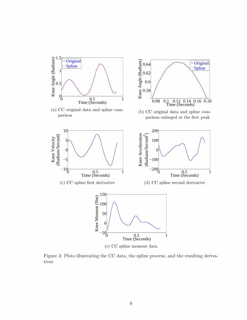
The original data was 55 samples long. To form a smooth representation

of the data, spline curves could be fit to it. This was completed using the spline

function in MATLAB, which uses cubic interpolation. Upon converting the raw data

to splines, a matrix of coefficients is generated, four coefficients for each time step, of

dimensions 54× 4. Multiplying this matrix by

0 3 0 0

0 0 2 0

0 0 0 1

0 0 0 0

yields the coefficients of the first derivative. Multiplying the coefficients of the first

derivative by the matrix once more produces the second derivative coefficient ma-

trix. It effectively reduces the order of the polynomial with each multiplication while

multiplying the remaining coefficients by the value of their associated powers. The

original (position), first derivative (velocity), and second derivative (acceleration)

splines could then be evaluated at the desired time step size. The results are illus-

trated in Figure 3. As desired, by using this method there is no noise introduced. To

complete the data set, the knee moment profile was processed by the same method,

though no derivatives were taken; it is also shown in Figure 3

8

0 0.5 10

0.5

1

1.5

Time (Seconds)

Kne

e A

ngle

(R

adia

ns)

OriginalSpline

(a) CC original data and spline com-parison

0.08 0.1 0.12 0.14 0.16 0.18

0.58

0.6

0.62

0.64

Time (Seconds)

Kne

e A

ngle

(R

adia

ns)

OriginalSpline

(b) CC original data and spline com-parison enlarged at the first peak

0 0.5 1−10

−5

0

5

10

Time (Seconds)

Kne

e V

eloc

ity(R

adia

ns/S

econ

d)

(c) CC spline first derivative

0 0.5 1−200

−100

0

100

200

Time (Seconds)

Kne

e A

ccel

erat

ion

(Rad

ians

/Sec

ond2 )

(d) CC spline second derivative

0 0.5 1−50

0

50

100

150

Time (Seconds)

Kne

e M

omen

t (N

m)

(e) CC spline moment data

Figure 3: Plots illustrating the CC data, the spline process, and the resulting deriva-tives

9

2.2 Veterans Administration Data Processing

For each trial the VA data was obtained in several forms, a marker and

force plate file resulting from motion capture, preprocessed joint trajectory (position

and velocity) files, a preprocessed file containing computed joint moments, and a

preprocessed file of the calculated joint powers. Each of the preprocessed files were

for a three-dimensional model. The usefulness of these files was limited, therefore,

because this work is to be completed for a two-dimensional model. It was determined

that the joint trajectories should be reevaluated in a two-dimensional framework.

Several pieces of information in particular must be obtained. These include the

dimensions of the subject, the joint trajectories, and a description of the heel and

toe forward kinematics. The data for the left leg was selected arbitrarily for these

computations.

2.2.1 Subject Dimensions

To begin the data analysis process, the subject dimensions must be deter-

mined from a standing trial. A marker set giving the global positions of the markers

during standing was provided for each subject. Frequently when evaluating the leg

in two dimensions, markers at the greater trochanter (GTRO), lateral epicondyle

(LEK), lateral malleolus (LM), heel (HEE), and fifth toe metatarsal (MT5) are used

as they sufficiently outline the subject’s leg position; refer to Figure 4. Accordingly,

these markers were used to determine the subject’s dimensions.

Six dimensions are of interest in defining the subject’s geometry. They are

the length of the thigh (l2), the length of the shank (l3), the length of the foot from

heel to toe (l4), the distance from the ankle joint to the toe (aT ), the distance from

the ankle joint to the heel (aH), and the height of the ankle joint above the sole of

10

−0.2 0 0.2 0.4 0.6 0.8 1

0

0.2

0.4

0.6

0.8

1

LEK

LMHEE MT5

Length (m)

Leng

th (

m)

GTRO

Figure 4: Marker placement for the leg

the foot (ah). These dimensions may be calculated by basic geometry.

l2 =√

(LGTROx − LLEKx)2 + (LGTROz − LLEKz)2 (2.1)

l3 =√

(LLEKx − LLMx)2 + (LLEKz − LLMz)2 (2.2)

l4 = LMT5x − LHEEx (2.3)

aT =√

(LLMx − LMT5x)2 + (LLMz − LMT5z)2 (2.4)

aH =√

(LLMx − LHEEx)2 + (LLMz − LHEEz)2 (2.5)

ah = LLMz −LMT5z + LHEEz

2(2.6)

The coordinate system for the global marker file is defined as x+ anterior and z+ up.

The L preceding each marker name indicates that it is for the left side. Because the

heel and toe markers were not consistently level, the average of the vertical coordinate

for each of these is used in determining the height of the ankle joint.

11

2.2.2 Position Data by Inverse Kinematics

Inverse kinematics provides the means of extracting joint translations and

rotations from motion capture marker data. In this case the vertical displacement

and rotation of the hip joint, rotation of the knee joint, and rotation of the ankle

joint are of interest. One method of solving motion capture data inverse kinematics

is to use optimization. A two-dimensional form of the method presented in [51] was

used to compute the inverse kinematics.

The global positions of the markers are known. A forward kinematics model

of the subject is created, and a matching marker set is placed on the model. The joints

of the forward kinematics model are then manipulated by the selected optimization

algorithm until by some measure of cost the forward kinematics model markers are

deemed close enough to the global positions recorded for the motion capture markers.

This process is completed for each time step of the motion capture data, eventually

providing a full set of joint trajectories. Within the next sections the forward kinemat-

ics model and optimization method will be developed for applying inverse kinematics

to the VA datasets.

Forward Kinematics Model

The forward kinematics model for the VA data had to be addressed consid-

ering two cases. Some trials consisted of walking in one direction on the treadmill

while others were reversed. This could be identified by the subject and marker set.

The direction was consistent among the trials of Subject AB01, who also had a full

body marker set recorded. All other subjects’ trials were in the opposite direction

and had only lower body marker sets recorded.

Local coordinate systems were defined for each segment of the leg. If the leg

is visualized resting in a horizontal orientation with the hip joint to the left and the

ankle joint to the right, each of the local coordinate systems may be simply defined

12

y

x

y

x

y

x

Figure 5: Local coordinate system assignment for forward kinematics

by placing their origins at the hip, knee, and ankle joints, pointing each x axis toward

the next origin, and pointing each y axis perpendicularly upward, Figure 5. The case

shown is for the direction traveled by Subject AB01. To be able to use the same

model for the alternative case, the vertical orientation of the foot may be reversed

while the coordinate systems remain in the same location and orientation.

To define any posture, the homogeneous transformation matrices for each of

these coordinate systems must be developed.

T (Tx, Ty, θ) =

cos(θ) − sin(θ) Tx

sin(θ) cos(θ) Ty

0 0 1

(2.7)

The inputs to (2.7) are a translation in the x direction Tx, a translation in the y

direction Ty, and a rotation θ. Each of the leg segment coordinate systems may be

described by using T .

Tthigh = T (Hiphoriz, Hipvert, Hiprot) (2.8)

Tthigh,shank = T (l2, 0, Kneerot) (2.9)

Tshank = TthighTthigh,shank (2.10)

Tshank,foot = T (l3, 0, Footrot) (2.11)

13

Tfoot = TshankTshank,foot (2.12)

Markers may now be placed in the frames that have been defined. The

global coordinates of each marker are generated by multiplying the coordinates of

the marker in the local coordinate frame by the related homogeneous transformation

matrix.

fhip(q) = Tthigh

[0 0 1

]T(2.13)

fknee(q) = Tthigh

[l2 0 1

]T(2.14)

fankle(q) = Tshank

[l3 0 1

]T(2.15)

fheel(q) = Tfoot

[−√aH2 − ah2 ∓ah 1

]T(2.16)

ftoe(q) = Tfoot

[√aT 2 − ah2 ∓ah 1

]T(2.17)

The sign of ah is selected based on the data set in use. For any trials related to

Subject AB01, it is negative. For all other marker data sets it is positive. The

positive case reverses the vertical orientation of the foot as was previously described.

Optimization

For this application the MATLAB function fminsearch was selected as the

optimization algorithm. The cost function was defined as a sum of the squared

residuals.

costIK =∑i

(markeri − fi(q))2 (2.18)

markeri represents the actual location of the markers, and fi(q) is the result of eval-

uating the forward kinematics model for marker i. An initial guess at approximately

standing was supplied to the algorithm for the first frame q = [0 1 − π/2 0 π/2].

After the first frame the solution of the previous time step was used as the initial

14

o0

y0x0

z0

q2

q3

q1

o2

o3

d0o1

m1

m2,l2

m3,l3

friction

g

x1

z1

z2

x2

z3x3

o3q4

Figure 6: Coordinate system assignment for the Cleveland State University hiprobot with prosthetic leg model attached. This figure was adapted from the orig-inally published version in [37] from IFAC-PapersOnline, DOI 10.3182/20140824-6-ZA-1003.00332, 2014. Used with permission, Appendix L

guess for each consecutive time step.

2.2.3 Coordinate System Alignment

The final step in processing the position data is aligning the data resulting

from the inverse kinematics computation with the coordinate system to be used in

simulation. The coordinate system for the simulation was determined through appli-

cation of the Denavit-Hartenberg convention for the Cleveland State University hip

robot combined with a knee and ankle prosthesis. It is defined as shown in Figure 6.

In all datasets the horizontal motion of the hip was discarded to match the constraints

15

0 500 1000 1500 2000 2500 3000 3500−2

−1.5

−1

−0.5

0

0.5

1

1.5

2

Frame Number

q

1 (m)

q2 (rad)

q3 (rad)

q4 (rad)

Figure 7: VA data trajectories for Subject AB01, Trial 003

of the robot. For the full body marker set cases all of the resulting inverse kinematics

required a change of sign to align with the coordinate system of Figure 6. The lower

body marker set cases required a reversal of the hip vertical displacement coordinate,

which was identical to the full body set, the addition of π to the hip angle coordinate,

and no changes to the remaining coordinates.

2.2.4 Velocity and Acceleration Data and Resampling

The computation of velocity and acceleration from the VA data was per-

formed by the same method as described in Section 2.1. Prior to the spline fit and

derivative process, however, the VA data’s sampling frequency was reduced by a fac-

tor of 3. This decrease in the number of samples provided a smoother fit because

every spline between points can increase the potential to fit the curve to fluctuations

due to noise. The resulting splines, including the position data, were evaluated at the

original sampling rate. Examples of the final trajectories for each of the joints after

this process may be seen in Figure 7.

16

aT aHah

o3

Figure 8: Foot dimension definitions and geometric relationships

2.2.5 Foot Kinematic Model

A triangular foot model was used throughout this work when ground contact

was of interest. This model is depicted in Figure 8. One may see that the foot model

connects to the sketch of the hip robot at the origin of the third coordinate frame.

The heel and toe coordinates may be located in the world frame (zeroth frame) by

kinematics. The forward kinematic equations for the x and z coordinates for both

the heel and the toe were derived as follows. These will be required in Section 4.1

x0h = l2 cos(q2)+l3 cos(q2+q3)+aH cos

(q2 + q3 + q4 +

(π

2+ cos−1

(ah

aH

)))(2.19)

z0h = q1 + l2 sin(q2) + l3 sin(q2 + q3)

+ aH sin

(q2 + q3 + q4 +

(π

2+ cos−1

(ah

aH

))) (2.20)

x0t = l2 cos(q2)+l3 cos(q2+q3)+aT cos

(q2 + q3 + q4 +

(π

2− cos−1

(ah

aT

)))(2.21)

z0t = q1 + l2 sin(q2) + l3 sin(q2 + q3)

+ aT sin

(q2 + q3 + q4 +

(π

2− cos−1

(ah

aT

))) (2.22)

17

2.3 Discussion

In brief, two separate data sets were prepared for use throughout this work.

The first set, the CC data, was composed of a single stride and required the process-

ing of derivatives. A spline-based method was applied and velocity and acceleration

determined. The second set from the VA included far more variety, ranging across

subjects and speeds and including multiple strides. It was reprocessed to fit the two-

dimensional requirement of this work. This included determining the dimensions of

subjects from marker data, calculating inverse kinematics, and defining some neces-

sary forward kinematics. The reference data is now formatted for use as a measure

of comparison and controller tracking reference.

18

CHAPTER III

ACTUATOR SYSTEM DESIGN AND

OPTIMIZATION

Unlike previous generations of prostheses, active prostheses require an ac-

tuator system. This system must comply with tight space constraints and generate

a significant amount of torque as it supports the weight of nearly the entire human

body for part of the gait cycle. In addition to these general requirements, the ultimate

goals of natural movement and optimal energy regeneration must be addressed.

For this work the actuator system is considered as any component in the

system starting from the joint of the prosthesis body up to and including the power

source. Accordingly, this is composed of both a mechanical and an electrical subsys-

tem. In this chapter the design methods for each of these systems is discussed followed

by simulation of, optimization of, and results for the overall actuator. The crank-slider

actuator is commonly modeled among prosthesis work. Also, supercapacitor-based

regenerative actuating mechanisms have been studied [33, 34, 37]. However, emphasis

on optimal energy regeneration through combining the crank-slider mechanism with

an electrical system including a supercapacitor is original to this work. The chapter

is concluded with a discussion.

19

Figure 9: Three-dimensional schematic of a direct drive actuator

3.1 Actuator Modeling

When designing a powered prosthesis, the system that transforms the out-

put of the motor to motion of the knee joint is an important consideration. One can

identify two primary methods, a geared direct drive mechanism and a crank-slider

mechanism, applicable to a knee joint. Within the broader context of powered pros-

thetics, it should be noted that both options may be applied to the ankle joint as

well.

Figure 9 depicts a schematic form of the first case, a direct drive actuator.

The only power transmission element between the motor and knee joint is the gearing.

Alternatively, Figure 10 represents a basic crank-slider mechanism. Power transmis-

sion in this case is accomplished by combining a motor, ballscrew, and linkage with

the knee joint.

A basic direct drive actuator model has been previously studied related to

this work [33]. Therefore, the crank-slider design was selected for investigation for

the sake of comparison and because of several notable features. Specifically, the

crank-slider design can fit conveniently within the shape of a human shank; it is

20

Figure 10: Three-dimensional schematic of a crank-slider actuator

compact. It is also a common form factor for prosthetics, making it possible to build

upon some previous work. Examples of prostheses using this architecture include the

Mauch SNS (passive), C-leg (passive with microcontroller), and Vanderbilt prototype

(active) [19, 46]. The ballscrew and linkage combination provides a wide range of

variables open to selection; this is of benefit because it offers multiple parameters

for optimization. Lastly, this design mimics the leg’s natural functioning as muscles

apply linear forces rather than direct torques to joints.

Development of the crank-slider actuator model was completed in two stages.

First, a proof of concept model mirroring a previous actuator model that included only

a geared direct-drive motor was completed. This was then followed by an expansion

of the crank-slider actuator model, integrating mechanical losses into the driving

mechanism to better evaluate the actuator’s capacity for energy regeneration.

3.1.1 Geometry and Kinematics

A symbolic expression describing the geometry, and thereby kinematics, of

the crank-slider is required. By rotating the entire assembly shown in Figure 10, a

convenient coordinate system for the crank-slider may be defined as shown in Fig-

21

Figure 11: Geometry definitions used in deriving crank-slider kinematics

ure 11, which illustrates the relevant nomenclature and is based on [29]. Referring to

the notation given in Figure 12, one can see that the flexion angle of the knee φk may

be directly related to θ2 by a constant angle φl, which is the angle at the knee joint

of the triangular link.

θ2 = π − φl − φk (3.1)

Figure 12: Notated three-dimensional schematic of crank-slider actuator

22

As further points of reference, a in Figure 11 is the side of that same triangular link

that joins the shank to the ballscrew, and d is the length of the shank between the

upper and lower crank-slider connection points.

Based upon Figure 11, loop equations for the x and y coordinates and a

geometric constraint equation may be established.

a cos θ2 − b cos θ3 − c cos θ4 − d = 0

a sin θ2 − b sin θ3 − c sin θ4 = 0

θ3 = θ4 + γ

(3.2)

Combining these equations and solving for θ2 and b yields the following.

θ2 = π + cos−1

(−a2 + b2 + 2bc cos γ + c2 − d2

2ad

)(3.3)

b =

√a2 − 2ad cos θ2 +

(c cos γ)2

2− (c sin γ)2

2− c2

2+ d2)− c cos γ (3.4)

Each of these equations will be utilized in the dynamic analysis, Section 3.1.2.

3.1.2 Dynamic Models

A representative dynamic model of the system is essential for optimization.

Because the primary interest of this work is energy regeneration, a modeling approach

based on power, which is easily integrated to evaluate energy, called bond graph mod-

eling was selected [21]. Furthermore, the desired result, the charging of a supercapaci-

tor, involves an interdisciplinary approach; the bond graph modeling method provides

a straightforward means of combining the mechanical and electrical engineering fields.

An overview of the bond graph approach is presented in Appendix A.

The bond graph modeling method is applied to the prosthesis actuator sys-

tem in several forms. First, the basic model for comparison to the direct drive model

23

Figure 13: Bond graph representing the basic actuator system

is developed. This is followed by two expansions to incorporate mechanical losses.

The first expansion involves the creation of a complex friction model for a selected

ballscrew to observe the effects of mechanical losses on the prosthesis’ energy regen-

eration capacity. The friction model is then generalized for use in optimization as the

second expansion.

Basic Actuator

While formalized bond graph construction methods have been developed,

the system of interest was constructed by inspection. The actuator model is shown in

Figure 13. The input SE on the left is a knee torque profile. From left to right, the

elements represent a torsion spring at the knee joint, crank-slider geometry, ballnut

mass, ballscrew lead, motor inertia, motor constant, armature resistance, an ideal DC-

DC power converter, and a capacitor. As can be seen in the figure, the modularity

of the bond graph method makes it simple to divide the system into the mechanical

and electrical subsystems for more detailed study and to expand the bond graph,

modeling further details.

Dividing the system at the GY element, thereby dividing it into the me-

chanical and electrical subsystems, one may consider the model at a deeper level.

Starting with the mechanical subsystem, the SE element represents the reference

data discussed in Section 2.1. This knee moment data accounts for all dynamic inter-

actions combined that apply torque to the knee joint. This is linked to a C element,

representing a torsion spring, such that they share the same velocity. The next el-

ement represents the crank-slider linkage. Recalling that the model is based on the

24

conservation of power, it is most straightforward to find the modulus G by writing

the power conservation equation across this element as follows:

Pin, knee (rotary) = Pout, ballscrew (linear)

T2θ2 = Fballscrewb

know, θ2 =db

dt

dθ2(b)

db= b

dθ2(b)

db

∴ Fballscrew =dθ2(b)

dbT2.

(3.5)

This equation provides the required relationship, and the derivativedθ2(b)

dbis G, which

is determined by taking the derivative of (3.3).

dθ2db

=b+ c cos γ

ad

√1− (−a2 + b2 + 2bc cos γ + c2 − d2)2

4a2d2

(3.6)

In addition to being used as the transformer modulus, the value of G describes the

instantaneous mechanical advantage of a given linkage.

The next several elements represent the ballscrew. First, the I element

stands for the ballnut’s linear inertia as it moves along the screw. Secondly, a trans-

former is used to represent the change from linear motion to rotation. The denomi-

nator of the modulus is the lead of the screw. Lastly, the rotational inertia element is

included in the mechanical subsystem. Within the model developed here, it represents

the motor inertia. The inertia of the ballscrew may also be added.

The transition to the electrical subsystem occurs at the GY element. The

modulus of this element is the motor torque constant. The circuit represented in the

bond graph is shown in Figure 14. A R element is placed in series with the motor

to represent the armature resistance. The DC-DC power converter is integrated into

the bond graph by use of an MTF element for which the transformer modulus is a

25

Figure 14: Circuit representing motor and electronics

value labeled u, which will be further discussed in Section 3.2. Lastly, a C element

represents one of the keys to the system, the supercapacitor energy storage device.

The causality assignment was such that the system state variables were the

knee velocity, motor momentum, and capacitor current. A through power convention

was also established. Consequentially, all elements will indicate power exiting the

system when the product of effort and flow is positive except the SE, which is the

opposite. The detail of deriving the system differential equations for simulation is

shown in Appendix B. The final result is given below:

φk = Glθm (3.7)

θm =1

Jm +ml2

(lGMk(t)− lGKφk −

α2

Rθm +

αu

RCqC

)(3.8)

iC =αu

Rθm −

u2

RCqC (3.9)

where φk is the knee angle, θm is the motor angle, qC is the capacitor charge, and iC

is the capacitor current.

Actuator with Complex Friction Model

Because the model of the basic actuator system is general for optimization

with the focus being placed on regeneration capacity, only the lead of the ballscrew

is being modeled as this incorporates both the kinematic and kinetic transformations

26

that this element implies. This is only one parameter that defines a ballscrew; the

remainder of the parameters, diameter, length, and preload among others, have been

left to be determined during future mechanical design beyond the scope of this work.

Accordingly, the ability to model mechanical friction is limited because few details

of the screw are known; however, to accurately consider the actuator’s potential for

energy regeneration, the mechanical losses must be estimated.

To address this challenge, a test case could be evaluated. An optimal set

of parameters can be determined with the basic actuator model, which is friction-

less. Within this parameter set a ballscrew lead value would be specified. A specific

ballscrew with this lead value could then be selected based on guidelines given by

ballscrew manufacturers and a complex friction model developed from the screw’s

now known parameters. This model can be simulated for a given parameter set,

providing insight into friction’s effects on the system’s power flow and energy usage.

Friction modeling within a ballscrew has been a topic of much study ranging

from the development of highly complex models to the simplest efficiency accounting.

Complex models of a ballscrew system includes variables such as rolling contact, lu-

brication, sliding, ball-to-ball contact, and the return system, among others, such as

in [30]. Simplifications modeling only a portion of these effects have been established.

For example, in [47] the model was based primarily on bearing-related effects. Consid-

ering the problem from a general perspective, it has been modeled with modification

as a basic screw as well [42]. Experimental modeling has also been applied to this

problem [20]. Selecting from among these options is really dependent on the accuracy

required for the application and the available information. For this work, reaching a

good balance between accuracy and available information, the method discussed in

[42] has been selected.

The addition of a complex friction model requires that another R element be

integrated into the actuator bond graph. According to [42], the friction of a ballscrew

27

Figure 15: Bond graph incorporating nonlinear R element that represents a complexfriction model for the ballscrew

is greatly dependent on the preload of the ballnut and primarily of the Coulomb type.

Φfric (f) = |τfric| sign (f) (3.10)

Φfric is a function of the incoming flow, angular velocity in this case, alone because

of the sign function. The addition of this function to the bond graph is illustrated

in Figure 15. It can be seen that this change to the bond graph does not change

the state variable definitions or add an algebraic loop, which would be indicated by

indefinite causality.

Due to the friction being primarily associated with the preload and com-

posed of the Coulomb form, the friction torque could be represented by the equation

typically describing the torque to raise or lower a load with the force FP set equal to

the preload rather than axial load force.

τfric = FPRpitch

(2πRpitchµ± l cosα

2πRpitch cosα∓ µl

)(3.11)

In addition to the preload, the pitch radius Rpitch, friction coefficient µ, screw lead

l, and thread angle α must be known. For a high-precision ballscrew with a light

preload in the ballnut a value of µ = 0.005 may be used for the coefficient of friction.

Additionally, the thread angle α for a ballscrew is 45o [42]. The remaining parameters

are dependent on the geometry of the specific ballscrew being considered. The first

set of signs given in (3.11) is for extension of the screw while the second set is for

28

compression.

Once again deriving the system equations in an algorithmic manner, the

final system describing the expanded model may be determined.

φk = Glθm (3.12)

θm =1

Jm +ml2

(lGMk(t)− lGKφk −

α2

Rθm +

αu

RCqC − Φfric

(θm

))(3.13)

iC =αu

Rθm −

u2

RCqC (3.14)

The details of this derivation are contained in Appendix D; it follows the derivation

of the frictionless system closely.

Actuator with Generalized Friction Model

Alternatively, and perhaps most commonly, the frictional losses of a ballscrew

can be modeled by a simplified method, accounting for the efficiency of the screw

which is stated by manufacturers to be about 90% [26]. The ballscrew friction model

developed by Olaru, et al. has shown close agreement with this value for a variety

of speeds and a range of contact loads, indicating the sufficiency of this method for

optimization purposes [30]. The results of the complex friction model should also

provide confirmation of this approach. Accounting for this efficiency figure in the

dynamic model provides a second means for modeling the ballscrew’s friction. Most

importantly, this approach is feasible for optimization as it is not dependent on screw

parameters beyond the lead l.

Applying this concept to the basic transformer model shown for the ballscrew

in Figure 13 requires a loss of the power conservation property of the bond graph as

illustrated in general terms for the case where the screw is converting power in the

29

mechanical rotation domain to power in the mechanical translation domain and η < 1.

Fscrewx = ητscrewθ (3.15)

The equations describing a ballscrew within a bond graph are separated into the

kinematic relationship and kinetic relationship, (3.16) and (3.17), respectively.

θ =1

lx (3.16)

τscrew = lFscrew (3.17)

Using these equations to substitute back into the right-hand side of the power equality

given in (3.15), one can see that the efficiency coefficient must only be applied to

either (3.16) or (3.17). Since the friction torque is a kinetic variable, it follows that

the efficiency coefficient should be applied to (3.17).

τscrew = ηlFscrew (3.18)

It cannot simply be said, however, that (3.18) always holds true as it is possible for

the screw to be driven by the force, backdriving.

Fscrew = η1

lτscrew (3.19)

For the power equality to hold for both of these cases and the equations to be of the

form (3.17) as implemented in the bond graph, the coefficient η cannot simply be set

to 0.9, though the efficiency is always 90%. The solution to this is to use the equation

of the form (3.18) where two values of η are switched between. The first is obvious:

ηF = 0.9 for the case where the force is driving the screw. The second is found by

solving (3.19) for τscrew. This requires ητ =1

0.9and is for the case where the torque

30

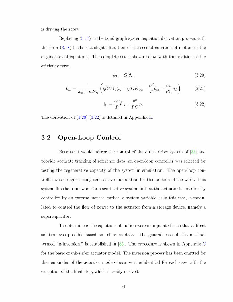
is driving the screw.

Replacing (3.17) in the bond graph system equation derivation process with

the form (3.18) leads to a slight alteration of the second equation of motion of the

original set of equations. The complete set is shown below with the addition of the

efficiency term.

φk = Glθm (3.20)

θm =1

Jm +ml2η

(ηlGMk(t)− ηlGKφk −

α2

Rθm +

αu

RCqC

)(3.21)

iC =αu

Rθm −

u2

RCqC (3.22)

The derivation of (3.20)-(3.22) is detailed in Appendix E.

3.2 Open-Loop Control

Because it would mirror the control of the direct drive system of [33] and

provide accurate tracking of reference data, an open-loop controller was selected for

testing the regenerative capacity of the system in simulation. The open-loop con-

troller was designed using semi-active modulation for this portion of the work. This

system fits the framework for a semi-active system in that the actuator is not directly

controlled by an external source, rather, a system variable, u in this case, is modu-

lated to control the flow of power to the actuator from a storage device, namely a

supercapacitor.

To determine u, the equations of motion were manipulated such that a direct

solution was possible based on reference data. The general case of this method,

termed “u-inversion,” is established in [35]. The procedure is shown in Appendix C

for the basic crank-slider actuator model. The inversion process has been omitted for

the remainder of the actuator models because it is identical for each case with the

exception of the final step, which is easily derived.

31

3.3 Simulation, Optimization, and Results

In this section the simulation and optimization methods and results of each

actuator model developed in Section 3.1.2 will be presented. Due to their consecutive

dependencies, the simulations, optimizations, and results will be grouped according

to model. Additionally, biogeography-based optimization, the optimization algorithm

selected for this work, will be discussed both theoretically and in application within

this section.

3.3.1 Basic Actuator

Simulation of Basic Actuator Model

The basic actuator model was developed in Simulink by implementing the

system equations (3.7)-(3.9) in block diagram form. An embedded MATLAB function

was used to contain the equations of the transformer modulus G. The input to the

system was the knee moment profile from the single stride CC data discussed in

Section 2.1.

In keeping with the parameters of the original direct-drive proof of concept

model, the parameters from the same motor datasheet, a Maxon RE 65, were used.

Because the ballscrew is an optimized element, the mass of the motor was substituted

for the value of the mass of the ballnut. Lastly, the link length c was set to zero,

reducing space requirements. Each of these parameters are detailed in Table I. The

remainder of the parameters were optimized and will be discussed in the following

sections on optimization.

Optimization of Basic Actuator Model

Optimization of the basic actuator model was completed to prove the poten-

tial for a crank-slider actuator to successfully charge a capacitor. The optimization

32

Parameter Symbol Value UnitsMotor Constant α 0.054 Nm/A

Armature Resistance R 0.0821 OhmMotor Inertia Jm 1.29× 10−4 kg m2

Estimated Nut Mass m 2.1 kgLink Length c 0 m

Table I: Fixed parameters for all actuator models

was accomplished with the biogeography-based optimization algorithm, which will be

described next. This is then followed by the detail of the application of biogeography-

based optimization to this particular problem.

Biogeography-Based Optimization Biogeography-based optimization

(BBO) is an algorithm based upon the migration and emigration of species to and

from various isolated habitats where the habitats represent problem solutions and

species characterize solution features [40, 41]. In nature each isolated habitat can

be labeled with an associated habitat suitability index (HSI), an overall measure of

its ability to support species. The HSI is dependent on a variety of suitability index

variables (SIV). Within the study of biogeography the SIV’s correspond to features of

a habitat such as the amount of vegetation, availability of water, climate, and other

factors.

Logically, if a habitat has a high HSI, it can support a greater number of

species and will, therefore, have a higher emigration rate, meaning that many species

will spread from the high HSI habitat to surrounding habitats. In addition, a high

HSI habitat will have a low immigration rate because it is so populated; most new

species will not have access to the necessary resources.

Transferring these general ideas to the solution of an optimization problem,

one can correlate each isolated habitat with a single candidate solution. The HSI is

a measure of candidate solution’s fitness. Similarly, the SIV’s correspond to features

of that candidate solution. Immigration λ and emigration µ rates are determined

33

Parameter ValuePopulation Size 200

Number of Generations 100Number of Elite Individuals 2

Probability of Mutation 0.02

Table II: Biogeography-based optimization parameters used for optimization of theactuator models

probabilistically and provide the means of sharing information between solutions.

The emigration rate determines whether or not a solution feature will be shared with

another habitat, and the immigration rate is used to select the future location of the

solution feature.

Beyond the basics of natural biogeography, two features are added to the

algorithm used in this work, mutation and elitism. Mutation is determined proba-

bilistically and set at a low rate such that new information may be added, reducing

the chance of the algorithm finding a local minimum, yet it does not become a random

search. To implement elitism the best candidate solutions are passed from generation

to generation; in this way the best solution of the consecutive generation will be no

worse than that of the previous generation.

Application of BBO to Basic Actuator Model Multiple optimization

runs were completed with the algorithm parameters given in Table II. A relevant cost

function was defined.

Cost = −(qC,final − qC,initial) (3.23)

Because BBO seeks to minimize the cost function and the goal is maximization of the

capacitor charge for one gait cycle, a negative sign is introduced. While maximization

of energy gain is more applicable, this cost function based on maximizing the capacitor

charge was selected to remain consistent with the original simulation [33].

The optimized parameters were selected as shown in Table III, which also

34

Parameter Minimum Value Maximum Value UnitsC 0 500 FK 0 100 Nm/rada 0 0.15 md 0 0.3 mγ 0 π radφl 0 π radl 1 6.350 mm/revqC0 0 8000 C

Table III: Optimization parameter ranges for the actuator models

includes the search spaces. All of the parameters were allowed to vary throughout a

continuous search space except for the ballscrew lead l for which a discrete set was

defined. This set consisted of the following values in mm/rev: 1, 1.25, 2, 2.5, 3, 4, 5,

5.08, 6, and 6.35. All values greater than and including 2 mm/rev are expected to

represent a backdrivable screw [49].

Lastly, several constraints were placed on the acceptable solutions to help

ensure basic feasibility. This was implemented through penalizing the cost function

of any solution not meeting the constraints by setting it to infinity. Specifically, the

geometry variables were required to result in real values for the variable length link

b (ballscrew) and for the transformer ratio G. Additionally, solutions for u resulting

from the u-inversion process were required to be real and between negative one and

one.

Results

Though multiple solutions were found following several optimization trials

that resulted in an increase in capacitor charge, one example set of results is provided

for the basic actuator model. Several considerations went into determining when

a sufficient set of parameters had been selected by the optimization algorithm as

the methods utilized do not guarantee global optima. These basic conditions were

applied for each case of optimization throughout this work. First, an intuitive sense

35

Parameter Symbol Value UnitsCapacitance C 221.54 F

Spring Constant K 47.64 Nm/radLink Length a 0.055 mLink Length d 0.25 m

Angle γ 1.32 radAngle φl 1.17 rad

Screw Lead l 5.08 mm/revInitial Capacitor Charge qC0 6726 C

Table IV: Example set of optimization results for the basic actuator model

for the capacity of the optimization was obtained through completing a number of

trials during the development of each model. Secondly, trials were performed with

the finalized model and any cost trends observed. Finally, as long as the algorithm

did not seek to exceed any of the parameter ranges and the cost functions were within

a relative measure of magnitude, the best cost solution was typically selected.

The parameters selected by the optimization algorithm are given in Table IV.

Each of these values are within feasible ranges. Figure 16 illustrates the minimum

value of the cost function from generation to generation. By 100 generations no visible

improvement has occurred in the cost function within the last forty generations, indi-

cating that this is a more than sufficient number of generations for this optimization

problem.

36

0 10 20 30 40 50 60 70 80 90 100−0.395

−0.39

−0.385

−0.38

−0.375

−0.37

−0.365

−0.36

Min

imum

Cos

t

Generation

Figure 16: Progression of the minimum cost for an optimization run for the basicactuator model for a single gait cycle

37

0 0.2 0.4 0.6 0.8 10

10

20

30

40

50

60

70

80

φ k (D

egre

es)

Time (Seconds)

ReferenceSimulated

Figure 17: Tracking performance of basic actuator model for single gait cycle

Mathematically perfect tracking is shown in Figure 17, indicating that the

open loop control method was successful. The total RMS error comparing the simu-

lated knee angle to the reference data

RMStotal =

√∑i

(φk,i,ref − φk,i,sim)2 (3.24)

was 7.52×10−5 rad. The electrical attributes of this trial for the complete stride may

be seen in Figures 18a–18c. For this set of parameters the capacitor charge increased

by 0.3932 C, and the energy increased by 11.94 Joules.

38

0 0.2 0.4 0.6 0.8 16724.5

6725

6725.5

6726

6726.5

Cap

acito

r C

harg

e q C

(C

oulo

mbs

)

Time (Seconds)

(a) Capacitor charge over one gaitcycle. An overall gain is observed.

0 0.2 0.4 0.6 0.8 130.354

30.356

30.358

30.36

30.362

Cap

acito

r V

olta

ge V

C (

Vol

ts)

Time (Seconds)

(b) Capacitor voltage over one gaitcycle. A slight increase in voltageis indicated

0 0.2 0.4 0.6 0.8 1−20

−10

0

10

20

Cap

acito

r C

urre

nt i C

(A

mps

)

Time (Seconds)

(c) Capacitor current over one gait cy-cle

Figure 18: Plots illustrating behavior of the basic actuator model electrical systemover one gait cycle

39

3.3.2 Complex Friction Actuator

Having shown that the crank-slider actuator at a basic level is capable of

energy regeneration, a model including friction at the ballscrew is to be simulated.

After describing the simulation, the results for the complex friction actuator model

are presented.

Simulation of Complex Friction Actuator Model

The complex friction actuator model simulation was created by using the

fixed parameter set and the parameter set identified during optimization of the basic

actuator model, Tables I and IV. To complete the model detail required for simulation,

an actual ballscrew must be identified. The selection of a ballscrew is primarily

dependent on the axial load. An equation expressing the axial load of the ballscrew

may be derived as implied by the bond graph:

Faxial =1

l

((ml2 + Jm

)θm +

α2

Rθm −

αu

RCqC

). (3.25)

This equation can be evaluated with the parameters of the presented basic actuator

system simulation results.

Upon evaluating (3.25), the peak force was extracted. The value determined

was Faxial = 1421 N ≈ 320 lbf. Coupled with the value of the screw lead, 0.2 in/rev

or 5.08 mm/rev, this information was sufficient to select a ballscrew as it also defined

the required preload value. The optimal preload value is 10% of the maximum force

according to [42]. This is a value of FP = 142.1 N ≈ 32 lbf. The selected screw must

be capable of having this preload applied.

A search was conducted among several ballscrew manufacturers. The final

selection was a PowerTrac 0631-0200 SRT RA screw and SEL 10408 nut assembly from

40

Nook Industries [18]. The datasheet for this product can be found in Appendix F.

This screw is able to handle a dynamic load of up to 815 lbf and preloads up to

233 lbf, and it possesses the required lead. While a ballscrew does not have a pitch

radius as defined in the typical sense for power screws or gears, the ball circle radius is

a reasonable approximation [17]. For the Nook Industries screw the ball circle radius

was Rpitch = 0.00801 m.

Simulink was used to create the system simulation. This was implemented

by constructing the system equations in block diagram form. While no optimization

was intended for this simulation, it was developed within the same framework as the

basic actuator simulation such that optimization could be possible if required in the

future given further development. Additionally, a specialized function was used to

implement the friction model. Within a MATLAB embedded function block logic

was assembled to provide switching between the screw extension and compression

variations of the friction torque equation and to apply the sign function.

Lastly, auxiliary MATLAB code was developed and additional blocks were

added to the Simulink diagram to track the power flow and energy usage of the

system. Alongside a general energy accounting an efficiency term for the ballscrew

was calculated. A sum of the power entering and a sum of the power exiting the

1-junction connecting the friction R element to the bond graph, excepting the power

entering the friction R element, were computed. These were integrated to determine

the total energy entering and exiting the junction. Division of the exiting energy

value by the entering energy value produced an efficiency term for the ballscrew. One

item of note within the energy balance software inconsequential to the final results is

discussed in Appendix G.

41

0 0.2 0.4 0.6 0.8 10

10

20

30

40

50

60

70

80

φ k (D

egre

es)

Time (Seconds)

ReferenceSimulated

Figure 19: Tracking performance of complex friction model for single gait cycle

Complex Friction Actuator Model Results

The simulation was run using the CC dataset for the input reference knee

moment with a length of one stride. Mathematically perfect tracking as predicted by

the u-inversion technique was attained, as shown in Figure 4. The total root mean

square value obtained, equation (3.24), was 7.9578× 10−5 rad.

The attributes of the electrical system throughout the simulation time are

depicted in Figures 20a–20c. With the inclusion of the friction losses the capacitor

still charged for the given parameter set. Over one full stride a gain of 0.2620 C was

observed.

42

0 0.2 0.4 0.6 0.8 16724.5

6725

6725.5

6726

6726.5

Cap

acito

r C

harg

e q C

(C

oulo

mbs

)

Time (Seconds)

(a) Capacitor charge over one gaitcycle. An overall gain is observed.

0 0.2 0.4 0.6 0.8 130.35

30.355

30.36

30.365

30.37

Cap

acito

r V

olta

ge V

C (

Vol

ts)

Time (Seconds)

(b) Capacitor voltage over one gaitcycle. A slight increase in voltageis indicated

0 0.2 0.4 0.6 0.8 1−20

−10

0

10

20

Cap

acito

r C

urre

nt i C

(A

mps

)

Time (Seconds)

(c) Capacitor current over one gait cy-cle

Figure 20: Plots illustrating behavior of the complex friction model electrical systemover one gait cycle

43

0 0.2 0.4 0.6 0.8 1−40

−30

−20

−10

0

10

20

30

∆ E

nerg

y (J

oule

s)

Time (Seconds)

∆ Human Input Energy∆ Spring Energy∆ Lin. Kinetic Energy∆ Rot. Kinetic Energy∆ Capacitor EnergyJoule LossesFriction Losses

Figure 21: Plot illustrating the change in energy of each component of the complexfriction model. For the given sign convention a negative change in energy correspondsto energy gained by a component

The change in energy for each component was also evaluated and is shown in

Figure 21. The sum of the final values of each component’s change in energy was on

the order of 10−6, confirming that the system model is truly energy conserving. An

overall gain of 7.95 J was observed in the capacitor. The net available energy entering

the system from the human was 26.58 J. The capacitor stored energy represents

approximately 30% of this available energy. It can also be noted that the losses

related to the motor resistance were two to three times greater than the friction

losses, suggesting that this may be an important area to investigate with respect to

the overall actuator’s efficiency.

The plot of power flow in Figure 22 shows an alternating pattern between the

power provided and required by the human and the power delivered to and extracted

from the capacitor. This illustrates the power exchange expected for regeneration.

Finally, the efficiency of the ballscrew actuator was evaluated, Figure 23.

44

0 0.2 0.4 0.6 0.8 1−600

−400

−200

0

200

400

600

Pow

er (

Wat

ts)

Time (Seconds)

Human Input PowerSpring PowerLin. Kinetic PowerRot. Kinetic PowerCapacitor PowerJoule Power LossesFriction Power Losses

Figure 22: Plot illustrating the power of each component of the complex frictionmodel. For the given sign convention a positive value corresponds to power enteringthe bond graph body, thereby exiting a component

At its lowest point the efficiency of the screw was 97%. This suggests that the

manufacturer’s value of 90% is more than sufficient in accounting for the friction

losses. However, it should be noted that the efficiency is dependent on the preload

of the ballscrew. While large variations in the required value of the preload are

not expected for different screws, further trials for different parameter sets would be

required to determine the range of this variation.

45

0 0.2 0.4 0.6 0.8 10.95

0.96

0.97

0.98

0.99

1

Bal

lscr

ew e

ffic

ienc

y, η

Time (Seconds)

Figure 23: Efficiency of the ballscrew within the complex friction actuator modelsimulated over one gait cycle

46

3.3.3 Generalized Friction Actuator

Having confirmed that the efficiency of the ballscrew is no less than 90%

by evaluating a more complex model of the ballscrew, it is reasonable to assume the

manufacturer’s given efficiency value of 90% to simplify the model. This simplification

makes optimization more feasible. It provides a means of creating an actuator model

that may be optimized yet will represent the frictional losses within a safe margin

of error. Within this section the simulation implementing the generalized friction

actuator model will be presented. This model will then be optimized. To conclude,

the results of this optimization will be presented.

Simulation of Generalized Friction Actuator Model

Similar to the simulation developed for the complex friction actuator model

the system equations were implemented in block diagram form. An embedded MAT-

LAB function was prepared for the selection of η. Based on the power convention of

the bond graph, the switching was defined such that η = 0.9 would be selected for

positive power flow through the ballscrew TF element, corresponding to backdriving,

and η =1

0.9would be selected for negative power flow, in which case the screw is

being driven by the torque. The value for η must be initialized due to requirements

of the simulation software. Because in the general case it is unknown which state the

simulation will begin in, the initial value for η was selected to be one, fully efficient

Code for an energy balance was completed for this model as well as calcula-

tion of the efficiency across the ballscrew TF element. While the system energy would

no longer balance because of the non-power conserving change made to the system

equations, the difference will represent the losses due to the screw’s friction torque. In

addition, dividing the time integral of the input power of the TF by the time integral

47

Optimized System Parameters

C(F)

K(Nm/rad)

a(m)

d(m)

γ(rad)

φl(rad)

l(mm/rev)

qC0

(C)

CapacitorChargeGained

(C)

CapacitorEnergyGained

(J)

FrictionLosses

(J)

Trial 1 122.89 32.32 0.061 0.30 0.49 1.32 5 4078 0.056 1.85 9.67Trial 2 140.82 31.16 0.091 0.23 2.43 1.35 2 4503 0.060 1.92 9.58Trial 3 70.39 32.18 0.061 0.30 0.58 1.32 5 2332 0.056 1.85 9.66Trial 4 117.40 32.15 0.062 0.30 2.26 1.33 5.08 3933 0.055 1.84 9.66Trial 5 151.62 30.69 0.036 0.29 2.71 1.28 3 4930 0.060 1.94 9.53

Table V: Optimization results for the generalized friction actuator model for five trials

of the output power of the TF will yield an efficiency term to be compared with the

expected value of 90%.

Optimization of Generalized Friction Actuator Model

Upon completion of the simulation, optimization of the generalized fric-

tion model could be accomplished. This was approached by use of the evolutionary

optimization algorithm biogeography-based optimization previously discussed. In ad-

dition to the basic algorithm, mutation and elitism were utilized once again. Each

run was begun with a random seed. Five trials were run with the algorithm parame-

ters of Table II. The parameter ranges defined in Table III were used for each of the

trials. All constraints were equivalent between the basic actuator model optimization

and the generalized friction actuator model optimization. The cost function was also

consistent with the basic actuator model optimization.

Generalized Friction Actuator Model Results

Associated with each trial a best parameter set was determined. The results

of the five trials are shown in Table V. While it cannot be concluded from the results

of the individual trials that a global optimum was found by the optimization algo-

rithm, it is clear that particular ranges of the parameters tend to cause the maximum

capacitor charge. The consistency across the capacitor charge gained, capacitor en-

ergy gained, and friction losses columns between trials is striking in that this suggests

48

0 10 20 30 40 50 60 70 80 90 100−0.06

−0.055

−0.05

−0.045

−0.04

−0.035

−0.03

−0.025

−0.02

Min

imum

Cos

t

Generation

Figure 24: Progression of the minimum cost for an optimization run for the general-ized friction actuator model for a single gait cycle

that even with the variations among the system parameters, the algorithm may have

been consistently approaching the same limit.

Example results will be provided for Trial 1. For each of the five optimization

runs convergence was achieved. An example plot is shown in Figure 24. Though the

greatest decreasing behavior occurs until generation 20, visible improvements may be

noted up to approximately generation 72. This indicates that 100 generations was

once again sufficient.

Because the timing of the efficiency switching could not be exactly deter-

mined during the u-inversion process for this case, the tracking, as shown in Figure 25,

is no longer mathematically perfect. The error of the simulated data versus the ref-

erence data according to equation (3.24) was RMStotal = 0.0011 rad. However, this

is still sufficient accuracy for gait.

49

0 0.2 0.4 0.6 0.8 10

10

20

30

40

50

60

70

80

φ k (D

egre

es)

Time (Seconds)

ReferenceSimulated

Figure 25: Tracking performance of generalized friction actuator model for single gaitcycle

50

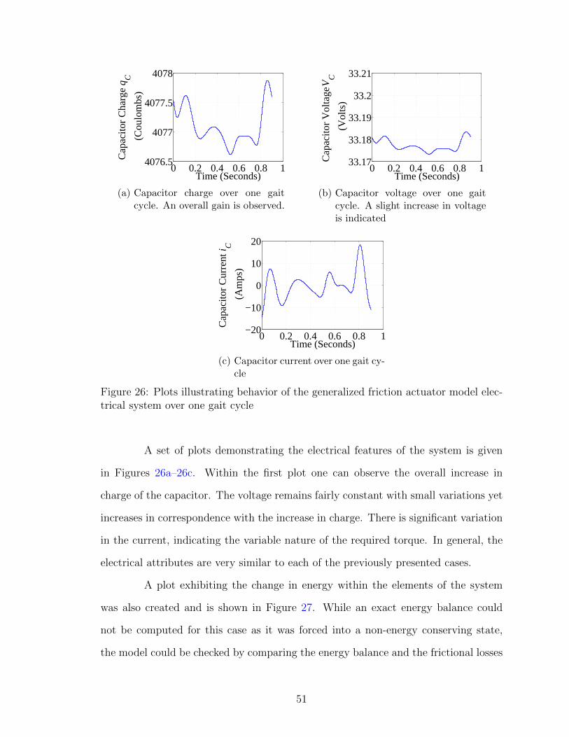
0 0.2 0.4 0.6 0.8 14076.5

4077

4077.5

4078

Cap

acito

r C

harg

e q C

(C

oulo

mbs

)

Time (Seconds)

(a) Capacitor charge over one gaitcycle. An overall gain is observed.

0 0.2 0.4 0.6 0.8 133.17

33.18

33.19

33.2

33.21

Cap

acito

r V

olta

ge V

C (

Vol

ts)

Time (Seconds)

(b) Capacitor voltage over one gaitcycle. A slight increase in voltageis indicated

0 0.2 0.4 0.6 0.8 1−20

−10

0

10

20

Cap

acito

r C

urre

nt i C

(A

mps

)

Time (Seconds)

(c) Capacitor current over one gait cy-cle

Figure 26: Plots illustrating behavior of the generalized friction actuator model elec-trical system over one gait cycle

A set of plots demonstrating the electrical features of the system is given

in Figures 26a–26c. Within the first plot one can observe the overall increase in

charge of the capacitor. The voltage remains fairly constant with small variations yet

increases in correspondence with the increase in charge. There is significant variation

in the current, indicating the variable nature of the required torque. In general, the

electrical attributes are very similar to each of the previously presented cases.

A plot exhibiting the change in energy within the elements of the system

was also created and is shown in Figure 27. While an exact energy balance could

not be computed for this case as it was forced into a non-energy conserving state,

the model could be checked by comparing the energy balance and the frictional losses

51

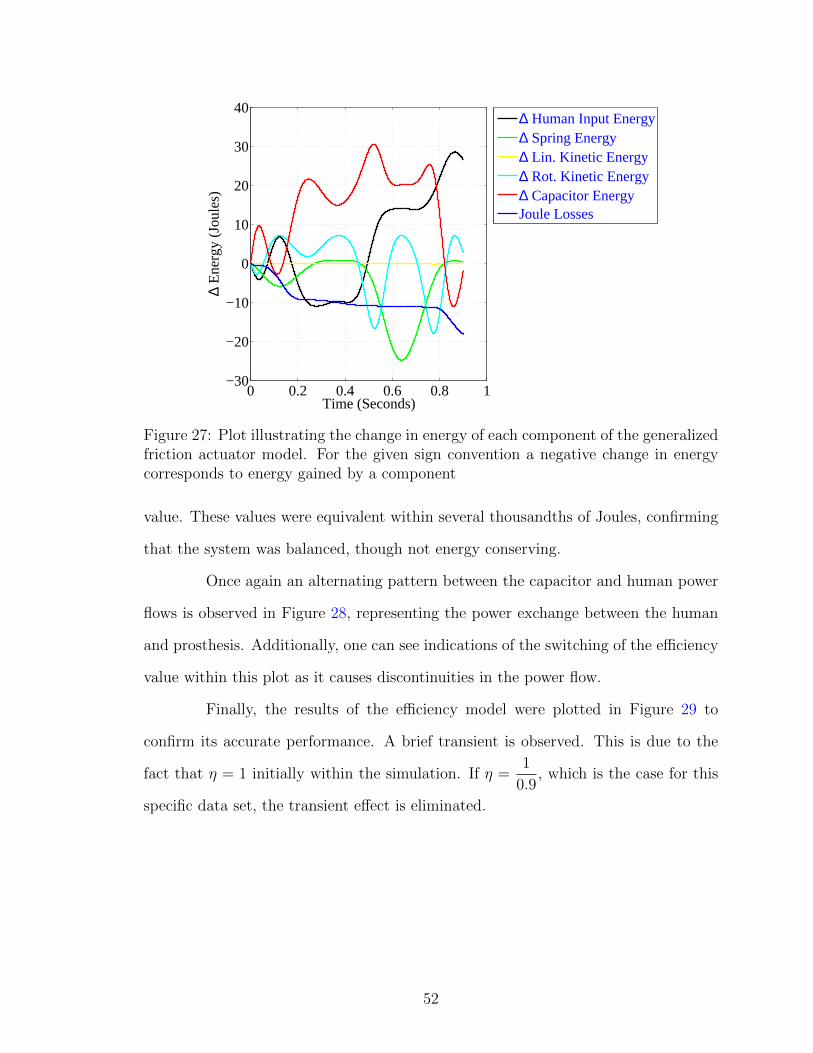
0 0.2 0.4 0.6 0.8 1−30

−20

−10

0

10

20

30

40

∆ E

nerg

y (J

oule

s)

Time (Seconds)

∆ Human Input Energy∆ Spring Energy∆ Lin. Kinetic Energy∆ Rot. Kinetic Energy∆ Capacitor EnergyJoule Losses

Figure 27: Plot illustrating the change in energy of each component of the generalizedfriction actuator model. For the given sign convention a negative change in energycorresponds to energy gained by a component

value. These values were equivalent within several thousandths of Joules, confirming

that the system was balanced, though not energy conserving.

Once again an alternating pattern between the capacitor and human power

flows is observed in Figure 28, representing the power exchange between the human

and prosthesis. Additionally, one can see indications of the switching of the efficiency

value within this plot as it causes discontinuities in the power flow.

Finally, the results of the efficiency model were plotted in Figure 29 to

confirm its accurate performance. A brief transient is observed. This is due to the

fact that η = 1 initially within the simulation. If η =1

0.9, which is the case for this

specific data set, the transient effect is eliminated.

52

0 0.2 0.4 0.6 0.8 1−800

−600

−400

−200

0

200

400

600

Pow

er (

Wat

ts)

Time (Seconds)

Human Input PowerSpring PowerLin. Kinetic PowerRot. Kinetic PowerCapacitor PowerJoule Power Losses

Figure 28: Plot illustrating the power of each component of the generalized frictionactuator model. For the given sign convention a positive value corresponds to powerentering the bond graph body, thereby exiting a component

10−3

10−2

10−1

100

0.9

0.92

0.94

0.96

0.98

1

Bal

lscr

ew e

ffici

ency

, η

Time (Seconds)

Figure 29: Efficiency of the ballscrew throughout one gait cycle

53

3.4 Discussion

Three individual models of a crank-slider actuator for an active prosthetic

leg were developed and validated within this chapter. First, a basic actuator model

mirroring a direct drive actuation system model from [33] was studied. The sec-

ond actuator model explored an approach to modeling the frictional losses of the

ballscrew based upon its geometry and preload. The final method was the implemen-

tation of generalized friction losses based upon an efficiency percentage, decoupling

the ballscrew geometry from the addition of friction to the simulation. This method

was pursued because it allows greater freedom in optimization; the ballscrew may

simply be modeled by its lead value as in the basic actuator model.

The basic actuator model showed the potential for this actuator style to

successfully collect excess energy at the knee joint across multiple optimization trials.

Among the three actuator models this model, which was without mechanical losses,

resulted in the greatest increase in capacitor charge, 0.3932 C.

The results of simulation of the complex friction actuator model indicated

that the manufacturer’s value of 90% efficiency is beyond sufficient as the lowest

value recorded for this model was approximately 97%. Additionally, for the specific

parameter set used in this simulation, regeneration capacity was maintained. The

second lowest increase in capacitor charge, this model showed a gain of 0.2620 C.

Looking to future development, the predicted regeneration capacity of the complex

friction model simulation is equivalent to 26% of the energy needed for driving an

ankle motor according to Winter’s data for a fast walking pace [52].

Simulation and optimization of the third model, the generalized friction

actuator model, was completed for a total of five trials. For many parameters a clear

range arose among the best solutions. Even at 90% efficiency the system was capable

of charging the capacitor. This model resulted in the smallest increase in capacitor

54

charge, a total of between 0.055 C and 0.060 C, dependent on the trial.

In summary, all three actuator models resulted in an increased capacitor

charge over one gait cycle of the CC reference data. With each consecutive increase

in the total friction modeled, a decrease in the accumulated charge is observed, pro-

viding confirmation of the models’ accuracy. One future direction for expansion of

this work is optimization of the motor and perhaps other aspects of the system to

decrease the losses due to the armature resistance, a multifaceted problem. Further

considering the energy regeneration capacity, it would be of interest to theoretically

determine the maximum limit possible and compare this value to the results achieved

through optimization. Additionally, looking toward physical application of the actu-

ator, machine design work must be completed. Finally, the models may be extended

and evaluated for the ankle joint of a fully actuated prosthesis.

55

CHAPTER IV

GROUND CONTACT MODEL DESIGN

AND OPTIMIZATION

In considering the development of a controller emphasizing energy regener-

ation, a broader model must be developed. Such a proposed model should include a

hip model in combination with a prosthesis model as well as a method of simulating

the effects of ground contact. A simulation of the Cleveland State University hip

robot and a Mauch prosthesis may be modified to address the first two requirements

and will be further discussed in Chapter V. A method of approaching the third and

final requirement, a ground contact model, will be addressed within this chapter.

As indicated in Figure 6, the hip robot operates in two dimensions. To

be applicable, the available reference data was processed down to two dimensions.

Therefore, it is required that any contact model developed for this case must also be

two-dimensional. Such a model has been previously implemented within the combined

hip robot-prosthesis simulation, yet its goal was solely replicating two-point, heel

and toe, contact with an approximately realistic magnitude for a single data set.

This limits its capacity to provide realistic ground reaction forces to the simulation

when any variation is introduced, consequentially limiting the ability to optimize a

controller across a variety of data.

56

In Section 4.1.1 the original contact model is reviewed, and a novel contact

model is developed in Section 4.1.2 to meet the aforementioned needs. Sections 4.2

and 4.3 are also unique contributions of this work. The methods used in optimizing

this model are described in Section 4.2. This is followed by Section 4.3, which presents

the results of the ground contact model optimization for several sets of test data.

Section 4.4 concludes the chapter with a discussion of these results.

4.1 Ground Contact Model

4.1.1 Initial Hip Robot Contact Model

The ground contact model original to the hip robot simulation as presented

in [28] was based on a spring and kinetic friction. A vertical force and a horizontal

force were each determined for both the heel and the toe. Because the treadmill is a

flexible walking surface, a spring model was selected for the vertical force calculation.

Observing the horizontal ground reaction force for the anterior-posterior direction,

Figure 30, one may note that it appears to be a scaled version of the vertical force

with a change in sign in the middle, leading to the general kinetic friction model with

a sign modification added.

According to a linear spring model

Fvert = −kbeltδvert (4.1)

the force is directly proportional to the compression of the spring; note that extension

past the spring’s equilibrium is not possible in this case. The vertical displacement

δvert is, practically speaking, the distance that the heel or toe dips beneath the tread-

mill “ground level.” It may be calculated by subtracting the vertical coordinate of

the heel or toe from the distance from the hip robot’s world origin to the treadmill

57

13 13.5 14 14.5−200

0

200

400

600

800

1000

Gro

und

Rea

ctio

n F

orce

(N

)

Time (Seconds)

VerticalHorizontal

Figure 30: Single stride example ground reaction force data from Subject AB01,Trial 003

surface, also called the standoff.

δvert = standoff− (heel or toe)vert (4.2)

Having determined the vertical force at both the heel and the toe, which is a nor-

mal force, the equation for kinetic friction may be applied directly to determine the

horizontal force for the heel and toe. The modification of the sign is handled as

shown.

Fhoriz = −∣∣∣µFvert∣∣∣sign

((heel or toe velocity)horiz − (belt velocity)

)(4.3)

The values assigned to each of the constants in the previous three equations are given

in Table VI.

58

Parameter Value Unitskbelt,heel 30000 N/mkbelt,toe 50000 N/m

standoff 1.03 mµ 0.2 unitless

Table VI: Parameters used in the initial hip robot contact model

4.1.2 Novel Ground Contact Model

The initial approach to developing a new contact model for use with a broad

array of data was based on an architecture identical to the model discussed in Sec-

tion 4.1.1 because in reality the closest model to a compliant belt is likely some form

of spring. Therefore, the initial model only differed from the original model in that

it included optimization (see Section 4.2 for algorithm details) of a threshold and a

stiffness constant for each the heel and the toe; the horizontal force model remained

the same. It should be noted that due to the method of processing the dataset of

Section 2.2, the definition of δvert is as shown in equation (4.4) from this point for-

ward. Here “threshold” is a small vertical shift dependent on the depth of ground

penetration required for sufficient contact.

δvert = threshold− (heel or toe)vert (4.4)

While this method did address the basic need, tuning the model to variable

data, it did not do so with good accuracy referred to the reference data. Particularly,

the results tended toward an overly extensive contact period, primarily before heel

contact is indicated to begin in the reference data, Figure 31c. Because the heel

was typically the source of this excess contact time, the heel force was frequently

minimized to unrealistically small values, Figure 31a.

59

13 13.5 14 14.50

10

20

30

Time (Seconds)

Gro

und

Rea

ctio

nFo

rce

(N)

(a) Heel

13 13.5 14 14.50

200

400

600

800

Time (Seconds)G

roun

d R

eact

ion

Forc

e (N

)(b) Toe

13 13.5 14 14.50

200

400

600

800

1000

Time (Seconds)

Gro

und

Rea

ctio

nFo

rce

(N)

SimulatedReference

(c) Total

Figure 31: Example vertical ground reaction force case resulting from optimizationof the contact model presented in Section 4.1.1 for Subject AB01, Trial 003

60

13 13.5 14 14.5−5

0

5

Gro

und

Rea

ctio

nF

orce

(N

)

Time (Seconds)

(a) Heel

13 13.5 14 14.5−200

−100

0

100

200

Gro

und

Rea

ctio

nF

orce

(N

)

Time (Seconds)

(b) Toe

13 13.5 14 14.5−200

−100

0

100

200

Time (Seconds)

Gro

und

Rea

ctio

nF

orce

(N

)

SimulatedReference

(c) Total

Figure 32: Example horizontal ground reaction force case resulting from optimizationof the contact model for Subject AB01, Trial 003

The results of the horizontal contact model are shown in Figure 32. These

results were deemed acceptable on several grounds. First, the overall magnitude was

accurate. Secondly, each of the positive and negative sections were represented over

the stride, though they were shifted. Lastly, the magnitude of the horizontal force

is small relative to the vertical force, decreasing its effects. Therefore, the same

horizontal contact force model was kept for all trials.

In an effort to improve upon the model, a number of variations with respect

to the spring were tested including quadratic, cubic, and quartic models. Not realizing

the desired change throughout these iterations suggested a fundamental shortcoming

of the model. Truly, the sole of the foot does not fit into solid body mechanics [53].

Rather, there is significant tissue before the “solid body” bone makes contact with

61

13 13.5 14 14.50

0.1

0.2

0.3

0.4

Hee

l Ver

tical

Posi

tion

(m)

Time (Seconds)

(a) Heel position. Note that sign isopposite world coordinate systemfor illustration purposes

13 13.5 14 14.5−2

−1

0

1

2

Hee

l Ver

tical

Vel

ocity

(m

/s)

Time (Seconds)

(b) Heel velocity. Note that sign is op-posite world coordinate system forillustration purposes

Figure 33: Example heel trajectories for Subject AB01, Trial 003

the ground. Numerous complex finite element models have been developed in the

study of the effects of foot structure on its loading [3, 10, 22]. Because of the time

required for optimization iterations, a faster method than finite element modeling is

required for this application. Furthermore, the level of detail and accuracy resulting

from such models would significantly exceed the requirements of this work. Hence

the addition of a damping term was considered as an alternative solution.

A damping force at a basic level can be considered velocity dependence,

paralleling a stiffness force which is displacement dependence. As the foot proceeds

through heel strike, see Figure 33, the vertical velocity decreases until solid contact,

full compression, of the heel at which point the velocity settles to practically zero.

Using this information, one may infer that damping, velocity dependence, could play

an important role in heel contact timing. One model illustrating a version of this

approach may be found in [1]. In this case a total of 10 spring-damper units are

spread across the surface of the sole of a two-dimensional foot model. Each element

follows

fy,j = aδ3j

(1 + bδj

). (4.5)

Within this equation fy,j is the vertical force at each element, a is the stiffness, b is

the damping, and δj is the distance by which the jth element penetrates the ground.

62

Because two contact points are to be used to replicate the ground reaction

force in this work as opposed to ten, the model from [1] still overcomplicates the

solution. Accordingly, an alternative model was developed, keeping this model in

mind. Considering the form of the data, refer to Figure 33, it follows that the higher

velocity corresponds primarily with soft tissue contact rather than compressed soft

tissue and bone. Therefore, an implementation of the damping approach that acts

as a valve or continuous switch, allowing less force through during higher velocity

periods and more force through during lower velocity periods, seems rational. This

may be implemented as shown below.

Fvert = −kbeltδvert(1− sat(bδ2vert, 0, 1)) (4.6)

Within equation (4.6) a linear spring determines the magnitude of the ver-

tical force, identical to the initial contact model. This is then multiplied with a term

that includes a saturation function, limiting its output to between zero and one. This

term either allows the full magnitude of the vertical force to pass or scales it back with

increasing velocity. If the velocity is too large, this term can reach zero, completely

eliminating the vertical force. The value b is the damping constant of a quadratic

form. δvert is the time derivative of equation (4.4). To take a smooth derivative of

δvert, a transfer function was utilized.

TFderivative =s

0.025s+ 1(4.7)

The value of 0.025 was selected by trial and error to maintain relative peak magnitudes

while providing a smooth result to avoid irrelevant switch action. The horizontal

contact model was maintained.

In summary, a novel contact model has been developed. It includes features

of the terrain, namely belt stiffness and friction, as well as a basis in the soft tissue

63

and bone combination influencing the sole of the foot. The next section will discuss

the selection of the constants associated with this model via optimization.

4.2 Contact Model Optimization

Because of the nature of the developed contact model, the constants sought

have not been previously defined in the literature. Additionally, adequate refer-

ence data is available. This combination fits well within an optimization framework.

Within Section 4.2.1 the selected optimization algorithm, particle swarm optimiza-

tion, will be presented. Particle swarm optimization was selected for this problem

since it is strong in both global and local exploration, an important feature because

little intuitive judgement could be used for initializing some of the parameters to be

optimized. Discussion of the method in general will be followed by the detail of how

particle swarm optimization was applied to the given problem, Section 4.2.

4.2.1 Particle Swarm Optimization

The particle swarm optimization (PSO) methodology is based upon the

swarming behavior of birds, fish, and other creatures. Each of these creature groups

have an optimal method of moving through space. Studies have indicated that each

individual’s movements are dependent upon both the individual’s preferred motion

and its neighbors’ trajectories. This combination of trends leads to the best overall

motion pattern for the group. Many forms of PSO have been developed based on this

generalized idea; only one version will be described here [6, 41].

Translating the swarm behavior into an algorithm, a population of candidate

solutions is initialized in two steps. First, each solution is given a starting position and

velocity. Secondly, the cost function for each candidate solution is evaluated. These

candidates are then sorted from best to worst, and the best individual is labeled the

64

current global best. A generational progression is then begun. At the start of each

generation the global best is identified and saved. For each candidate solution its

personal best is updated if its current position is an improvement on the past best,

and its neighborhood best is identified. The neighborhood for this version of PSO is

being defined as a particular number of nearest individuals; the number of individuals

in the neighborhood is a tuning parameter of the algorithm [41].

Identification of each best is followed by an update of each individual’s

velocity

∆vpersonal,i = r1,i φ1,max (vpersonal best,i − vcurrent,i)

∆vneighborhood,i = r2,i φ2,max (vneighborhood best,i − vcurrent,i)

∆vglobal,i = r3,i φ3,max (vglobal best,i − vcurrent,i)

vnew,i = κ (vcurrent,i + ∆vpersonal,i + ∆vneighborhood,i + ∆vglobal,i) ,

(4.8)

where i refers to the index of the individual in the PSO population. The first three

equations describe the change in velocity caused by the three components, personal,

neighborhood, and global bests. The difference between each best and the current

velocity is multiplied by a random number r scaled by φmax such that the value is

between zero and φmax. Each φmax is a tuning factor for the algorithm; in ascending

order they are termed the cognitive constant, the neighborhood social constant, and

the global social constant. Within the final equation all of the velocity change factors

are added to the current velocity. This sum is scaled by κ, the constriction coefficient;

it prevents the velocity from reaching unstable magnitudes and is calculated as shown,

where α is a tunable parameter [41].

κ =2α

φ1,max + φ2,max + φ3,max − 2(4.9)

Upon determining the velocity of each individual, the new velocity is added

65

to the current position. These values are then bounded by a given range, which has

been defined for the problem. The cost is once again calculated, and the population

is sorted from best to worst. A form of elitism is then implemented by replacing the

global worst by the global best, concluding the generation. The process is replicated

for each generation until a stopping criterion is met. In these ways the candidate

solutions are scattered over the solution space, performing a global search, and yet

are drawn to the best overall solution, performing a local search as the generations

progress [41].

4.2.2 Contact Model Optimization

The equations describing the contact model were recreated in block diagram

form within Simulink. The forward kinematics for the heel and toe were computed

and then fed into these force equations, specifically vertical and horizontal forces

were calculated for both the heel and the toe. It should be noted that damping

was implemented for both contact areas, heel and toe. Though not discussed earlier,

damping was applied to the toe because of the potential for soft tissue effects across

the complete sole of the foot. The optimization was left to determine the usefulness

of this parameter. In the case that the toe did not require this degree of freedom, b

could be set to zero. As in the original contact model µ was set to 0.2. The primary

output of the simulation for optimization was the sum of the vertical heel and toe

forces, the total vertical force.

The PSO algorithm described in Section 4.2.1 was wrapped around this

simulation, which produced the data required to evaluate the cost function

RMS =

√1

n

∑j

(GRFref,j −GRFsim,j)2, (4.10)

where j refers to the sample number in the time interval of interest. With exception of

66

Parameter ValuePopulation Size 50

Number of Generations 75Number of Elite Individuals 1

Neighborhood Size 5φ1,max 2φ2,max 2φ3,max 2α 0.9

Table VII: Particle swarm optimization parameters used for optimization of the con-tact model

Parameter Minimum Value Maximum Value Unitsthreshold −0.1 −0.03 mkheel −1000000 −1000 N/mktoe −1000000 −1000 N/mbheel 0 2000 s2/m2

bknee 0 100 s2/m2

Table VIII: Optimization parameter ranges for the contact model

the number of generations, the PSO algorithm parameters were selected by reference

to the literature [41]. The number of generations was determined by observation of the

convergence behavior. The PSO parameter values are given in Table VII. For each of

the parameters being varied within the simulation, ranges were set by observation of

the reference data and trial and error. The final selected set is provided in Table VIII.

Optimization was setup to be performed over a single, user-selected stride of data from

toe-off to toe-off.

4.3 Results

Optimization of the contact model was conducted across three human sub-

jects and at up to three speeds, yielding a total of nine datasets. In each case the

PSO algorithm showed suitable convergence behavior within the specified 75 gener-

ations, Figure 34. Though in most cases small improvements not visible within the

67

0 10 20 30 40 50 60 70 8050

100

150

200

250

300

350

400

Min

imum

Cos

t

Figure 34: Example convergence curve for PSO optimization of the contact model forSubject AB01, Trial 003

plot continued to be made until the final generation, the average cost (not shown)

was approaching near the minimum cost, indicating convergence.

The dataset from Subject AB01 included only preferred speed data; two

trials from this set were used for optimization. The dataset from Subject AB03

included multiple trials at three different speeds, fast, preferred, and slow. Two trials

at each speed were selected and optimized. It should be noted that the marker data

for Subject AB01 yielded a fairly level foot. For AB03 a slight tip downward toward

the toe is distinguishable. The dataset for AB04 is included because this dataset had

a comparatively larger difference in height between the heel and toe markers, a factor

of interest. The optimization is nondeterministic, therefore a set of representative

results was selected after multiple optimization runs for each dataset. It was found as

a general rule that a cost function value of approximately 90 N, give or take, indicated

the potential for a suitable solution. The optimization process indicated a number of

local minima. A summary of the example solutions is given in Table IX.

A trend to eliminate the toe damping is seen throughout all of the trials,

68

Subject Trial Speed

Optimized Contact Model ParametersSolution Cost

(N)threshold

(m)kheel

(N/m)ktoe

(N/m)bheel

(s2/m2)btoe

(s2/m2)

AB01 003Preferred

1 m/s−0.0597 6752 36058 101.49 5.31 73.99

AB01 004Preferred

1 m/s−0.0574 32481 61706 101.45 0 71.01

AB03 00017Fast

1.25 m/s−0.0501 21013 48292 82.35 0 106.88

AB03 00018Fast

1.25 m/s−0.0534 22038 41490 1984.73 0 117.47

AB03 00001Preferred

1 m/s−0.0570 5134 38985 1745.38 6.15 90.82

AB03 00002Preferred

1 m/s−0.0549 1888 39511 0 3.31 91.23

AB03 00011Slow

0.75 m/s−0.0448 110536 90664 2000 0 101.53

AB03 00012Slow

0.75 m/s−0.0539 13263 48573 854.27 0 92.72

AB04 0001Preferred1.3 m/s

−0.0382 289695 60117 1877.43 0 127.74

Table IX: PSO optimization results for the contact model across multiple data sets

suggesting that this is not as significant a factor for the toe as opposed to the heel.

Additionally, it may be noted that the lowest cost solutions (AB01) are associated

with a more level heel and toe marker set, indicating that this may be a somewhat

limiting factor of the contact model; see Figure 35. Beyond these broad remarks,

some of the given solutions will be highlighted to note several more features of the

results.

Comparing the application of the contact model with damping to the op-

timization results shown in Figure 31 from optimization of the original model, one

may note that while there is still a period of slight heel stubbing, Figure 36, the

damping effect allows the optimization process to increase the heel force, Figure 36a,

without a large penalty. The peak heel force is increased by a factor of five in this

case. Additionally, the toe makes contact quickly after heel strike, and the heel leaves

contact prior to toe off, both features of gait.

69

0.4 0.60

0.1

0.2

0.3

0.4

34 5

34 5

Len

gth

(m)

Length (m)

(a) AB01

−0.4 −0.2 00

0.1

0.2

0.3

0.4

345

345

Leng

th (

m)

Length (m)

(b) AB03

0.2 0.4 0.60

0.1

0.2

0.3

0.4

34

5

34

5

Len

gth

(m)

Length (m)

(c) AB04

Figure 35: Example inverse kinematics plots illustrating the progression of subject’stendencies toward a sloped foot. Each frame was frozen when the subject’s hip markerwas directly over his or her ankle marker

13 13.5 14 14.50

50

100

150

Time (Seconds)

Gro

und

Rea

ctio

nFo

rce

(N)

(a) Heel

13 13.5 14 14.50

200

400

600

800

Time (Seconds)

Gro

und

Rea

ctio

nFo

rce

(N)

(b) Toe

13 13.5 14 14.50

200

400

600

800

1000

Time (Seconds)

Gro

und

Rea

ctio

nFo

rce

(N)

SimulatedReference

(c) Total

Figure 36: Example vertical ground reaction force case resulting from optimizationof the contact model for Subject AB01 at his or her preferred walking pace, Trial 003

70

14 14.5 15 15.50

100

200

300

Time (Seconds)

Gro

und

Rea

ctio

nFo

rce

(N)

(a) Heel

14 14.5 15 15.50

200

400

600

800

Time (Seconds)

Gro

und

Rea

ctio

nFo

rce

(N)

(b) Toe

14 14.5 15 15.50

200

400

600

800

1000

Time (Seconds)

Gro

und

Rea

ctio

nFo

rce

(N)

SimulatedReference

(c) Total

Figure 37: Example vertical ground reaction force case resulting from optimizationof the contact model for Subject AB03 at a fast walking pace, Trial 00017

Within the next set of results shown, Figure 37, a brief period of toe stubbing

is observed, indicating that the threshold was not low enough. Features such as this

are far more common for marker sets where the heel marker is higher than that of

the toe, such as is the case for the marker placement for Subject AB03.

The optimization of AB04 presented three cases, significant toe stubbing,

complete elimination of heel contact, and an increase of the threshold and heel stiff-

ness. Each of these served the purpose of improving the cost under “toe-dipped”

conditions. The third case was most prevalent among the solutions and was, thereby,

selected for inclusion in the presented data, Figure 38. It can be seen that the greatest

effect of the non-level foot for this example dataset is the limited heel contact period.

71

11.5 12 12.5 13 13.50

200

400

600

Time (Seconds)

Gro

und

Rea

ctio

nFo

rce

(N)

(a) Heel

11.5 12 12.5 13 13.50

200

400

600

800

Time (Seconds)G

roun

d R

eact

ion

Forc

e (N

)(b) Toe

11 12 13 140

200

400

600

800

1000

Time (Seconds)

Gro

und

Rea

ctio

nFo

rce

(N)

SimulatedReference

(c) Total

Figure 38: Example vertical ground reaction force case resulting from optimization ofthe contact model for Subject AB04 at his or her preferred walking pace, Trial 0001

72

4.4 Discussion

A contact model for use with two-dimensional data has been developed and

tested. The goal was to form a model that could be optimized for use with the

hip robot simulation and a variety of datasets. Heel contact was improved over the

original model by introducing damping, velocity dependence. The model was tested

over nine different datasets in each case providing a workable solution, though some

would be preferred. It was also shown through this process that the damping effect

was of greater importance at the heel, which is the location of greatest impact during

gait, in comparison to the toe.

It can be seen across the results that a true double-peaked solution was

not obtained. It is likely due to the fact that the heel force, though increased, is

still low in comparison to the literature. Though heel and toe forces are not easily

measured separately, resistive devices and pressure mats can provide a comparison

of magnitude. These values suggest that the peak heel force should be less than

that of the toe force yet reach between two-thirds and three-quarters of the peak

toe force [2, 27, 32]. Future modifications to improve the magnitude of the heel

contact may include changing the form of the damping portion of the equation or

integrating several spring models, such as using both linear and quadratic types.

Implementing the contact model within a dynamic simulation with closed loop control

may also improve the force profile because the forward kinematics driven approach

does not react to contact. By extension, the optimization of the contact model could

be completed within a dynamic simulation.

The model is also limited by its ability to adapt to marker sets in which the

heel and toe markers are not practically level. While a working solution could still

be generated in these cases, it is rarely realistic. Because variation in the placement

of markers is common, this issue will be ongoing. Anatomy would suggest that the

73

variation being seen is due to the placement of the heel marker because there is greater

freedom at this location of the body as opposed to the toe. To limit the effects of

this, the addition of an offset to the heel marker data, approximately leveling the heel

and toe, when defining the subject dimensions and prior to the inverse kinematics

computation may be possible.

These limitations being considered, the contact model is still consistent in

its replication of heel strike, toe off, and the overall magnitude of the force relative

to the reference data. Therefore, it is sufficient for use in dynamic simulations where

these items are of primary importance such as will be required in Chapter V.

74

CHAPTER V

CONTROL SYSTEM DESIGN AND

OPTIMIZATION

Robust tracking/impedance control has been recently introduced as a con-

troller for systems that include both joints that should be controlled by a tracking

strategy and joints that should be more pliable, combining tracking with force control

[28]. Additionally, a form of impedance control with gain scheduling has been pre-

sented in the past as a reliable means of controlling a transfemoral prosthesis [45, 46].

The first controller has been tested with a single dataset on the same general model

as is being used within this work [28]; however, the gains were hand tuned and the

emphasis was not on energy regeneration. The second controller also appeared to be

tuned without reference to energy regeneration.

In this chapter the combination of and expansion upon the robust track-

ing/impedance controller and the gain-scheduled impedance control work is sought

in two ways. First, the robust tracking/impedance controller will be applied to the

complete system, and the gait cycle will be broken into several sections. For each

individual section, as appropriate, a set of gains will be defined. Secondly, the gain

set will be optimized using multiple objectives, including energy regeneration.

Sections 5.1–5.3 cover precedent research. In Sections 5.4–5.6 new contri-

75

butions are communicated. The dynamic model of the hip robot and prosthesis is

conveyed in Section 5.1. In Section 5.2 the robust tracking/impedance controller

will be described. The gain-scheduled impedance control work will be covered in

Section 5.3. Upon establishing each individual controller, the method proposed of

combining the two will be discussed, Section 5.4. Next, Section 5.5 will present the

details of the optimization. This will be followed by results, Section 5.6. A discussion,

Section 5.7, will conclude.

5.1 Hip Robot and Prosthesis Dynamic Model

A dynamic model of the hip robot and a prosthesis was obtained for testing

of the controller in simulation. This model is developed in detail up to the ankle joint

in [36]. Several modifications and the addition of a foot model have been made since

that publication. Some of these changes are reflected in [28]. Further adjustments for

use in this work have also been made; therefore, the model will be briefly described

in this section.

Of greatest importance among the changes made to the model is the addition

of a foot model. This development was originally completed by the author of [28],

and it was then modified for this work. The foot is of the form shown in Section 2.2.5.

The forces applied to the foot are determined according to the contact model given

in Section 4.1.2. The effects of these forces at each of the four joints, hip translation,

hip rotation, knee rotation, and ankle rotation, are then calculated by use of the

transpose of the Jacobians for the heel (h) and the toe (t).

F1,h

τ2,h

τ3,h

τ4,h

= JTv,h

Fhoriz,hFvert,h

(5.1)

76

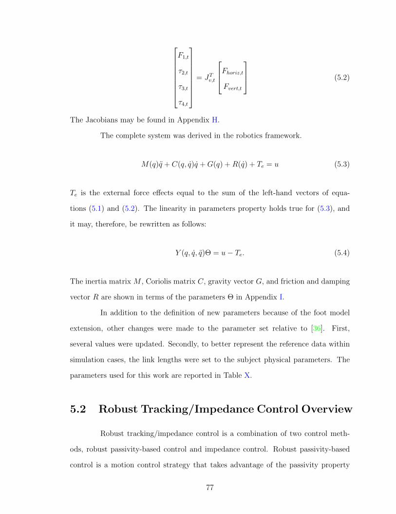
F1,t

τ2,t

τ3,t

τ4,t

= JTv,t

Fhoriz,tFvert,t

(5.2)

The Jacobians may be found in Appendix H.

The complete system was derived in the robotics framework.

M(q)q + C(q, q)q +G(q) +R(q) + Te = u (5.3)

Te is the external force effects equal to the sum of the left-hand vectors of equa-

tions (5.1) and (5.2). The linearity in parameters property holds true for (5.3), and

it may, therefore, be rewritten as follows:

Y (q, q, q)Θ = u− Te. (5.4)

The inertia matrix M , Coriolis matrix C, gravity vector G, and friction and damping

vector R are shown in terms of the parameters Θ in Appendix I.

In addition to the definition of new parameters because of the foot model

extension, other changes were made to the parameter set relative to [36]. First,

several values were updated. Secondly, to better represent the reference data within

simulation cases, the link lengths were set to the subject physical parameters. The

parameters used for this work are reported in Table X.

5.2 Robust Tracking/Impedance Control Overview

Robust tracking/impedance control is a combination of two control meth-

ods, robust passivity-based control and impedance control. Robust passivity-based

control is a motion control strategy that takes advantage of the passivity property

77

Parameter Symbol Value UnitsMass of link 1 m1 40.5969 kgMass of link 2 m2 8.5731 kgMass of link 3 m3 2.29 kgMass of link 4 m4 1.0875 kg

Length of link 2 l2 Subject thigh length mLength of link 3 l3 Subject shank length mLength of link 4 l4 Subject foot length m

Length joint 1 to link 2 CG c2 0.09 mLength joint 2 to link 3 CG c3 0.32 mLength joint 3 to link 4 CG c4 l4/2 m

Rotary inertia of link 2 I2z 0.435 kg-m2

Rotary inertia of link 3 I3z 0.0618 kg-m2

Rotary inertia of link 4 I4z 0.0184 kg-m2

Link 1 sliding friction f 83.33 NLink 2 rotary damping b 9.75 N-m-s

Table X: Parameter values used in the combined hip robot and prosthesis simulation.CG stands for center of gravity

of the robotic equations and is capable of handling parameter uncertainties, which is

particularly important in live implementation [43]. Impedance control is a means of

controlling force and velocity’s relationship [14, 15, 16]. A controller combining these

two approaches is desirable for the system of Section 5.1 because the upper two joints,

hip vertical displacement and hip rotation, are required to follow set trajectories, pure

motion control, while the prosthesis, knee and ankle joints, should be more flexible

while yet following reference data. In this way the natural motion of a human hip is

enforced regardless of the force and torque requirements on the hip robot. Further,

the prosthesis, because in implementation it is not part of the natural system, may

be tuned to act and react more like a human leg. This divides the system’s joints

into motion controlled (MC) joints q1 and q2 and impedance controlled (IC) joints

q3 and q4 [28]. The general control method, particularly the way in which these two

control strategies are interrelated, will be presented next, leaving proof of the method

to [28].

78

First, the desired impedance is described.

I ¨qIC + b ˙qIC + kqIC = −TIC (5.5)

q is the tracking error and TIC is the external force and moment effects. Diagonal

matrices I, b, and k are the desired impedance values. The control is then defined in

the form utilized in robust passivity-based control.

u = M(q)a+ C(q, q)v + g −Kr + TIC (5.6)

K is a diagonal matrix of four gains. The first two values of K are for MC joints,

and the last two values are for IC joints. This may also be expressed as in the form

indicating linearity in the parameters. Θ will be discussed later.

u = Y (q, q, v, a)Θ−Kr + TIC (5.7)

According to robust passivity-based control, v, a, and r are defined as follows.

vMC = qdMC − ΛMC qMC (5.8)

aMC = v = qdMC − ΛMC˙qMC (5.9)

rMC = q − v = ˙qMC + ΛMC qMC (5.10)

For the impedance controlled joints v, a, and r include an extra term.

vIC = qdIC − ΛIC qIC − Frz (5.11)

aIC = v = qdIC − ΛIC˙qIC − Frz (5.12)

79

rIC = q − v = ˙qIC + ΛIC qIC + Frz (5.13)

Λ is a diagonal matrix composed of four elements, as seen in the motion control set

of equations for v, a, and r and the impedance control set of equations for v, a, and

r. It is divided into two diagonal matrices, ΛMC and ΛIC , composed of two elements

relative to each set of v, a, and r. The term added to v, a, and r is the product of

a gain matrix Fr and a dynamic compensator. The dynamic compensator is a state

equation with the state z.

z = Az +KpqIC +Kd˙qIC +KfTIC (5.14)

Fr, Kp, and Kd may be calculated from the selected impedance gains. Justification

for these values is provided in [28].

Fr = I−1 (5.15)

Kp = k + AIΛIC (5.16)

Kd = b− IΛIC + AI (5.17)

At this point Θ may be determined according to the robust passivity-based control

framework.

Θ = Θ0 + δθ (5.18)

δθ is a switching term that is determined by a Lyapunov argument [28]. The result-

ing definition for δθ is prone to chattering, and therefore a deadzone solution was

implemented rather than the original version. The deadzone version is given below

80

[28].

δθ =

−ρ Y T r

||Y T r||,∣∣∣∣Y T r

∣∣∣∣ > ε

−ρεY T r,

∣∣∣∣Y T r∣∣∣∣ ≤ ε

(5.19)

In applying this controller to the hip robot and prosthesis model there are

a total of 14 gains to be tuned. There are two values of K and two values of Λ for

the motion control joints, two values of K and two values of Λ for the impedance

control joints, and lastly, the three impedance values, I, b, and k, for each of the two

lower joints. Ten of these gains are associated with the prosthetic joints. All were

originally tuned by trial and error.

5.3 State-Based Gain Switching

An alternative control method for prostheses also based on impedance con-

trol has been developed. In this case the control equation is simpler, but the gains

are switched according to a finite state machine based on measurable features of the

gait cycle. The controller was implemented for both the knee and ankle joints and

tested with an active prosthesis prototype [45, 46].

Consisting of a spring term, a damper term, and an equilibrium angle, the

impedance controller is defined.

τi = ki(θ − θki) + biθ (5.20)

i is the index of the current state as determined by a finite state machine. As opposed

to the model presented in Section 5.2, this model does not include an inertia term.

The most recent version of the finite state machine includes a total of five

modes. These modes are early stance, middle stance, late stance, swing flexion, and

swing extension. The flow between these states and the corresponding transitions

81

Figure 39: Finite state machine used for switching of control gains. Reproduced from[45]. c© 2011 IEEE

are depicted in Figure 39. Each of the measurements required to transition between

states are dependent only upon data that could be obtained from the prosthesis,

making them hardware-feasible selections.

Considering a total of five states, three parameters per control law, and two

joints, there is a total of 30 control gains requiring tuning for this method. Initial

tuning was completed via a least squares fit against reference torque, angle, and

angular velocity profiles. Further tuning was completed by hand during prototype

testing.

5.4 Switched Robust Tracking/Impedance Controller

The controllers discussed in Sections 5.2 and 5.3 both have merit with re-

spect to the human system. In the robust tracking/impedance controller it is assumed

that a human will use his or her residual limb the same as before his or her amputa-

tion. Additionally, in both cases the application of impedance control implements the

capacity to respond to the environment in a dynamic fashion. Within the gain sched-

uled impedance controller the fact that humans do not present a constant impedance

during dynamic action is applied [24]. Taking each of these features and combining

82

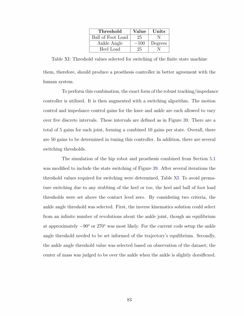
Threshold Value UnitsBall of Foot Load 25 N

Ankle Angle −100 DegreesHeel Load 25 N

Table XI: Threshold values selected for switching of the finite state machine

them, therefore, should produce a prosthesis controller in better agreement with the

human system.

To perform this combination, the exact form of the robust tracking/impedance

controller is utilized. It is then augmented with a switching algorithm. The motion

control and impedance control gains for the knee and ankle are each allowed to vary

over five discrete intervals. These intervals are defined as in Figure 39. There are a

total of 5 gains for each joint, forming a combined 10 gains per state. Overall, there

are 50 gains to be determined in tuning this controller. In addition, there are several

switching thresholds.

The simulation of the hip robot and prosthesis combined from Section 5.1

was modified to include the state switching of Figure 39. After several iterations the

threshold values required for switching were determined, Table XI. To avoid prema-

ture switching due to any stubbing of the heel or toe, the heel and ball of foot load

thresholds were set above the contact level zero. By considering two criteria, the

ankle angle threshold was selected. First, the inverse kinematics solution could select

from an infinite number of revolutions about the ankle joint, though an equilibrium

at approximately −90o or 270o was most likely. For the current code setup the ankle

angle threshold needed to be set informed of the trajectory’s equilibrium. Secondly,

the ankle angle threshold value was selected based on observation of the dataset; the

center of mass was judged to be over the ankle when the ankle is slightly dorsiflexed.

83

5.5 Controller Optimization

The BBO algorithm was selected for the tuning of the switched robust track-

ing/impedance controller. A composite cost function including tracking, ground re-

action force, and energy regeneration was prepared. To bring each component into

a general range of magnitude such that each would have an equal chance of being

minimized, weights were applied.

cost = q3,cost + q4,cost +1

100E3,cost +

1

200GRFvert,cost

q3,cost =

√1

n

∑i

(q3,i,sim − q3,i,ref )2

q4,cost =

√1

n

∑i

(q4,i,sim − q4,i,ref )2

E3,cost =

∣∣∣∣∣∣(E3,t2,sim − E3,t1,sim)−t2∫t1

P3,refdt

∣∣∣∣∣∣GRFvert,cost =

√1

n

∑i

(GRFvert,i,sim −GRFvert,i,ref )2

(5.21)

where i is the time index of each point in the time interval of interest. Each of the

tracking costs and the GRF cost are in root mean square form. The energy cost is

calculated such that the change in energy over the simulated gait cycle will approach

the total excess of energy available at the knee, determined by integration of the

knee power reference data. The energy cost was defined to approach the reference

energy because the capacity to gain or lose energy is directly related to the joint

torque, assuming the velocity is fixed by accurate tracking performance. Therefore,

if realistic torque values are met for the actuation system, it is technically possible

for the energy to increase by an amount greater than would be indicated by human

reference data. The cost to this, however, is the potential for high reaction forces or

84

Parameter ValuePopulation Size 50

Number of Generations 200Number of Elite Individuals 2

Probability of Mutation 0.02

Table XII: Biogeography-based optimization parameters used for optimization of theswitched robust tracking/impedance controller

Parameter Minimum Value Maximum ValueΛ3 or ΛIC,1 1 4000

K3 1 4000I3 0.01 6b3 1 6000k3 1 75000

Λ4 or ΛIC,2 1 4000K4 1 4000I4 0.01 6b4 1 3000k4 1 75000

Table XIII: Optimization parameter ranges for the robust tracking/impedance con-troller. The gains for the knee joint are in the upper portion while the ankle jointgains compose the lower half

torques at other joints, making a limit desirable.

BBO was applied in the same form as was discussed in Section 3.3.1. The

BBO algorithm parameters were set as given in Table XII for each run. The popu-

lation size was selected based on the number of individual parameters to be varied.

After several iterations the number of generations was determined according to the

observed rate of convergence. Each population member included a set of 50 gains,

those previously described. For each of the 10 gains per state ranges within which the

population features could be varied were set; refer to Table XIII. The population was

initialized randomly within these ranges with exception of two candidate solutions,

one high impedance case and one low impedance case from [28]. To define these

gains for use in the multiple state switching format, the gains were repeated for each

state, forming a 50 gain candidate solution. These initial candidates are presented

85

Parameter Initial Candidate 1 Initial Candidate 2Λ3 or ΛIC,1 230 230

K3 350 350I3 0.1 0.9b3 150 500k3 1000 3000

Λ4 or ΛIC,2 300 300K4 550 550I4 0.1 0.9b4 30 250k4 400 2000

Table XIV: Initial optimization candidate solutions for the robust tracking/impedancecontroller. The table is divided by grouping the knee joint gains in the upper portionand the ankle joint gains below

Hip Joint Gain ValueΛ1 or ΛMC,1 155Λ2 or ΛMC,2 155

K1 155K2 150

Table XV: Gains used for the hip joint

in Table XIV. Lastly, the gains of the hip motion controller, none of which were

being optimized, were selected to provide accurate tracking; see Table XV. Though

iterations were not completed, it was found that the gains related to the hip verti-

cal displacement q1 could be reduced relative to those selected in [28]. The values

associated with the hip rotation q2 were maintained from [28].

Any gain combinations that resulted in divergence were penalized by forcing

them to have a cost value of infinity. Such solutions were caught by two methods.

The first method was composed of a try/catch statement. If a solution diverged

within simulation causing it to throw an error, it would be caught at this level. The

second method was post-simulation as a divergent solution did not guarantee that

the simulation would crash. These solutions were caught by calculating the difference

between consecutive values of q4. If the absolute value of this difference was greater

86

Evaluative Measure Trial 1 Trial 2 Trial 3 Trial 4 Trial 5q3,cost (rad) 0.006352 0.007332 0.004612 0.012917 0.003954q4,cost (rad) 0.009355 0.008636 0.009565 0.004577 0.010621E3,cost (J) 0.0011 0.0491 0.0404 0.0044 0.0010GRFcost (N) 51.01 54.41 52.33 59.12 51.86

cost 0.2708 0.2885 0.2762 0.3131 0.2739∆E3 (J) 9.5639 9.6141 9.6054 9.5606 9.5640

Table XVI: Cost function and energy results for five optimization trials

than 10 degrees, the solution was penalized with an infinite cost. In practice a number

of solutions would be penalized early in the generational progression. The number

of penalized solutions would then decrease as the population improved throughout

ongoing generations. These methods were found sufficient across all trials.

Due to the lengthy computation time required for this optimization, five

trials were able to be completed. The data from Subject AB01 Trial 003 and related

contact model were used across all trials. While the state switching method is capable

of self-initialization during multiple stride trials, it was initialized by hand because

of the single stride data being used in each trial. The results of these trials will be

presented in the next section.

5.6 Results

Across five trials the final cost measures and amount of energy gained were

remarkably consistent. These results are summarized in Table XVI. The accuracy of

the tracking error is sufficient for gait across all trials. In comparison to the contact

model for Subject AB01 Trial 003, GRFcost has made significant improvement as well.

According to integration of the precalculated power data from the VA dataset, the

available energy at the knee is 9.565 J for Subject AB01 Trial 003, which each of

the solutions approaches as desired. To further evaluate the detail of the results,

examples will be provided from Trial 1. The convergence behavior of the minimum

87

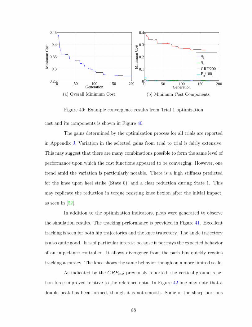
0 50 100 150 2000.25

0.3

0.35

0.4

0.45

Generation

Min

imum

Cos

t

(a) Overall Minimum Cost

0 50 100 150 2000

0.1

0.2

0.3

0.4

Generation

Min

imum

Cos

t

q3

q4

GRF/200E

3/100

(b) Minimum Cost Components

Figure 40: Example convergence results from Trial 1 optimization

cost and its components is shown in Figure 40.

The gains determined by the optimization process for all trials are reported

in Appendix J. Variation in the selected gains from trial to trial is fairly extensive.

This may suggest that there are many combinations possible to form the same level of

performance upon which the cost functions appeared to be converging. However, one

trend amid the variation is particularly notable. There is a high stiffness predicted

for the knee upon heel strike (State 0), and a clear reduction during State 1. This

may replicate the reduction in torque resisting knee flexion after the initial impact,

as seen in [52].

In addition to the optimization indicators, plots were generated to observe

the simulation results. The tracking performance is provided in Figure 41. Excellent

tracking is seen for both hip trajectories and the knee trajectory. The ankle trajectory

is also quite good. It is of particular interest because it portrays the expected behavior

of an impedance controller. It allows divergence from the path but quickly regains

tracking accuracy. The knee shows the same behavior though on a more limited scale.

As indicated by the GRFcost previously reported, the vertical ground reac-

tion force improved relative to the reference data. In Figure 42 one may note that a

double peak has been formed, though it is not smooth. Some of the sharp portions

88

13 13.5 14 14.5−0.94

−0.92

−0.9

−0.88

Time (Seconds)

q 1 (M

eter

s)

SimulatedReference

(a) Hip Displacement

13 13.5 14 14.560

80

100

120

Time (Seconds)

q 2 (D

egre

es)

SimulatedReference

(b) Hip Angle

13 13.5 14 14.50

20

40

60

80

Time (Seconds)

q 3 (D

egre

es)

SimulatedReference

(c) Knee Angle

13 13.5 14 14.5−120

−100

−80

−60

Time (Seconds)

q 4 (D

egre

es)

SimulatedReference

(d) Ankle Angle

Figure 41: Example tracking results from Trial 1 optimization

13 13.5 14 14.5−200

0

200

400

600

800

1000

Time (Seconds)

Ver

tical

GR

F (

N)

SimulatedReference

Figure 42: Example vertical GRF results from Trial 1 optimization

89

13 13.5 14 14.50

1

2

3

4

Time (Seconds)

Cur

rent

Sta

te

Figure 43: Example state switching results from Trial 1 optimization

of the GRF curve may be associated with the diversions of the ankle joint from its

intended trajectory.

Based upon the previously presented figures, one may consider the accuracy

of the state switching method. The timing of the states is presented in Figure 43. No

bouncing between states is observed. Each of the states are dwelt upon for a period

of time.

In designing a controller one must consider the required control efforts. Fig-

ure 44 illustrates the control signal profiles. The preprocessed three-dimensional

estimates of the required joint effort may be used to provide a baseline comparison

between these control torques and those used by the human subject. This data is

available for the hip torque, knee torque, and ankle torque. A peak magnitude of

27 Nm is given for the hip torque. The control signal peak is multiples larger than

the reference. Comparing the peak knee torque to the reference peak, it is more than

ten times the magnitude of the reference value, 44 Nm. The peak ankle torque, ignor-

ing the instantaneous spike, is consistently less than the reference peak, 160 Nm. It

is possible that this is related to the fact that the ankle showed the most impedance

controlled-like behavior.

90

13 13.5 14 14.5−1000

−500

0

500

Time (Seconds)

u 1 (N

)

(a) Hip Control Force

13 13.5 14 14.5−400

−200

0

200

400

Time (Seconds)u 2 (

Nm

)

(b) Hip Control Torque

13 13.5 14 14.5−200

0

200

400

600

Time (Seconds)

u 3 (N

m)

(c) Knee Control Torque

13 13.5 14 14.5−200

0

200

400

Time (Seconds)

u 4 (N

m)

(d) Ankle Control Torque

Figure 44: Example control signal results from Trial 1 optimization

91

13 13.5 14 14.5−20

−10

0

10

20

30

40

Time (Seconds)

∆ E

3 (J)

Figure 45: Example ∆E3 results from Trial 1 optimization

Lastly, the energy profile was evaluated. It is shown in Figure 45. The

general shape of the profile is fairly consistent with the result of integrating the

reference power data, though the magnitude is greater because it is dependent on u3.

Furthermore, the timing of the largest positive change in energy corresponds with the

latter part of swing phase. There is also an small increase associated with the early

portion of stance phase. These are two of the typical periods when excess energy is

typically dissipated. The other significant rise is early swing phase as the gait cycle

approaches toe off. The remainder of the shape is associated with various periods of

energy usage [52].

5.7 Discussion

Two ideas that have each been previously applied to prosthesis control,

namely robust tracking/impedance control and switched impedance control, have

been combined. The resulting controller was optimized. Throughout the process and

92

within the results it is clear that there is much room for further development.

There are multiple limitations to the modeling process. While the model was

expanded to use the limb lengths of the subject rather than all robotic parameters, the

masses, locations of the centers of mass, and moments of inertia remained unchanged

from the original robot model. It may be due to these inconsistencies that some

results of the simulation do not match the reference data better.

In addition, the control efforts, particularly those associated with the hip

joint, have the potential of being high because of the tuning of the tracking portion

of the controller. The goal of such a controller is following a trajectory regardless of

external influences. Therefore, excessive force or torque may be used.

Improvements of the optimization portion of this work may be addressed

in several ways. First, an excessive amount of computation time was required for

one trial. By estimation this time may be reduced by at least a factor of 10 on a

24 core computer. Development of the optimization within a formal multi-objective

framework may also be beneficial. By this means the balance of objectives could be

more easily defined. Finally, extending the optimization across multiple gait cycles

would encourage robustness of the controller.

In conclusion, the switched robust tracking/impedance controller was suc-

cessful in meeting each of the proposed optimization goals. Accurate tracking was

obtained in simulation. GRF was also realistic. Lastly, the excess energy typically

seen within a natural knee joint was replicated, providing the opportunity to consider

energy regeneration within lower limb prostheses.

93

CHAPTER VI

CONCLUSIONS AND FUTURE WORK

In conclusion, the goal of completing several steps in the design process

of an electrically regenerative active knee and ankle prosthesis has been met. A

complete crank-slider actuator system traversing from knee joint to supercapacitor

has been evaluated and proven its capacity for energy regeneration in simulation. This

process was completed in three consecutive models. First, a basic model to consider

energy regeneration within the crank-slider actuator was optimized and validated.

Secondly, a model including a screw geometry-based friction function was evaluated

and indicated energy regeneration even with the inclusion of mechanical losses. Lastly,

a generalized mechanical loss term was introduced in place of the complex friction

function to form an actuator that could be optimized while yet including mechanical

losses. This model also resulted in successful energy regeneration. The succession

of these actuator models provides support for the possibility of using a crank-slider

actuator to drive a prosthetic knee joint while harvesting energy.

To consider the controller of a prosthesis within a simulation environment

ranging from the natural hip joint to contact with the ground, an improved two-

dimensional ground contact model was completed. A contact model dependent on

constant threshold and stiffness values was included within the combined hip robot

and prosthetic leg simulation. While the approach was sufficient in the original case,

94

it was not adaptable to a variety of reference data sets. This low level of flexibility

led to the development of a novel ground contact model. In addition to developing

a method of optimizing the contact model for each subject and dataset, a damping

term was added to the ground contact model to facilitate a more natural level of heel

contact force and better timing of the heelstrike condition. The resulting contact

model proved sufficiently accurate to use in a two-dimensional simulation of the leg

for controller testing.

Lastly, a novel control strategy for the leg was presented. In this controller an

established method, robust tracking/impedance control, was used as the foundation,

and the known variable impedance of the human system was added by considering

a previously developed impedance switching prosthesis controller. Implementation

consisted of the hip joint of the hip robot and prosthesis system being driven solely by

a robust passivity-based controller and the knee and ankle joints being controlled by

the robust/tracking impedance controller. The gains for the two lower joint controllers

were determined through a state switching algorithm with a total of five states. These

gains were optimized for tracking at the knee and ankle joints, ground reaction force

tracking, and energy regeneration. Across five trials good tracking was obtained along

with the desired energy regeneration.

Future Work

In addition to the improvements mentioned under each individual topic there

are several broader opportunities for future work. First, the contact model and con-

troller may be extended to describe and handle stairs, slopes, and other terrain. This

process would consist of several steps. Reference data for any task of interest must be

collected and processed in a two-dimensional framework. This would be followed by

defining the threshold as a function of the data that could be vertically shifted rather

than shifting solely a constant. For slopes such a function could easily be a line. For

95

steps and other terrain it may need to be defined piecewise. New optimizations would

then be required according to dataset to determine the contact model parameters.

Extending the simulation in this way provides a means to test the prosthesis design

across a variety of activities of daily living.

Each of the optimizations performed should be formally evaluated for pa-

rameter sensitivity. For example, within the actuator system portion of this work it is

possible that the capacitance may not effect energy regeneration. Furthermore, there

is a level of dependence between the geometric parameters of the crank-slider design.

Completion of such an analysis would provide insight into the effects of each param-

eter and perhaps provide a means of reducing the number of optimization variables.

Also, the actuator model may be transposed into the combined hip robot

and prosthesis simulation. For the knee joint this process may be completed with the

actuator model’s current formulation. Adjustments to the model to align coordinate

systems would be required to add the actuator to the ankle joint. This combination

would change the control variable from joint torques to the transformer modulus u,

introducing the semi-active modulation method of control in both joints. Alongside

the development of the actuator system, a power management system design must

be prepared. Such a system, generally speaking, should control the transfer of energy

in and out of multiple capacitors, particularly from the knee to the ankle. A battery

is also a likely component within this system as a self-powering state is unlikely,

especially considering high energy expenditure activities such as climbing a flight of

stairs.

Combined with mechanical design work, the resulting model could then

be prototyped. Following the creation of a prototype, experimental testing of the

switched robust tracking/impedance controller may be completed with use of the hip

robot hardware, making further validation of the simulations of this work possible.

Successful testing with the hip robot would lend itself to testing with an able-bodied

96

subject by use of a bent-leg adapter. The goal would then be to progress to clinical

testing with amputees.

Finally, it has been shown in the literature that the impedance displayed

at human joints is a continuous variable [24]. Accordingly, the switching of the

controller may be extended into a continuous function. This may be a function of both

kinematic and kinetic variables at the joints. A significant amount of further study

and likely experimental work would be required to better classify this function and

successfully reproduce it within a controller. Mirroring able-bodied joint impedance

should further the objective of producing able-bodied gait through a prosthetic leg.

Each of these extensions will take the ideas presented in this work a step closer to an

energy regenerative, powered transfemoral prosthetic system capable of replicating

natural gait.

97

BIBLIOGRAPHY

[1] Marko Ackermann and Antonie van den Bogert. Optimality principles for model-

based prediction of human gait. Journal of Biomechanics, 43(6):1055–1060, April

2010.

[2] Thierry Chevalier, Helen Hidgins, and Nachiappan Chockalingam. Plantar pres-

sure measurements using an in-shoe system and a pressure platform: A compar-

ison. Gait & Posture, 31(3):397–399, March 2010.

[3] Snehal Chokhandre, Jason Halloran, Antonie van den Bogert, and Ahmet

Erdemir. A three-dimensional inverse finite element analysis of the heel pad.

Journal of Biomechanical Engineering, 134(3):031002–1–031002–9, March 2012.

[4] Steven Collins and Arthur Kuo. Recycling energy to restore impaired ankle

function during human walking. PLoS One, 5(2):e9307, February 2010.

[5] Juan Dixon, Ian Nakashima, Eduardo Arcos, and Micah Ortuzar. Electric vehicle

using a combination of ultracapacitors and ZEBRA battery. IEEE Transactions

on Industrial Electronics, 57(3):943–949, March 2010.

[6] Russell Eberhart and James Kennedy. A new optimizer using particle swarm

theory. In Proceedings of the Sixth International Symposium on Micro Machine

and Human Science, pages 39–43, Nagoya, Japan, 1995.

98

[7] Centers for Disease Control and Prevention. Number (in thousands) of hospital

discharges for nontraumatic lower extremity amputation with diabetes as a listed

diagnosis, United States, 1988-2009, 2012. http://www.cdc.gov/diabetes/

statistics/lea/fig1.htm, accessed July 14, 2015.

[8] Robert Gailey, Kerry Allen, Julie Castle, Jennifer Kucharik, and Mariah Roeder.

Review of secondary physical conditions associated with lower-limb amputation

and long-term prosthesis use. Journal of Rehabilitation Research & Development,

45(1):15–29, 2008.

[9] Joost Geeroms, Louis Flynn, Rene Fabian, Bram Vanderborght, and Dirk

Lefeber. Ankle-knee prosthesis with powered ankle and energy transfer for CY-

BERLEGs α-prototype. In Proceedings of the IEEE International Conference

on Rehabilitation Robotics, pages 1–6, Seattle, Washington, June 2013.

[10] Amit Gefen, Michal Megido-Ravid, Yacov Itzchak, and Mircea Arcan. Biome-

chanical analysis of the three-dimensional foot structure during gait: A basic tool

for clinical applications. Journal of Biomechanical Engineering, 122(6):630–639,

July 2000.

[11] Andrew Gitter, Joseph Czerniecki, and Kelly Weaver. A reassessment of center-

of-mass dynamics as a determinate of the metabolic inefficiency of above-knee

amputee ambulation. American Journal of Physical Medicine & Rehabilitation,

74(5):332–338, 1995.

[12] Brian Hafner, Laura Willingham, Noelle Buell, Katheryn Allyn, and Douglas

Smith. Evaluation of function, performance, and preference as transfemoral

amputees transition from mechanical to microprocessor control of the prosthetic

knee. Archives of Physical Medicine and Rehabilitation, 88(4):207–217, April

2007.

99

[13] Zach Harvey, Benjamin Potter, James Vandersea, and Erik Wolf. Prosthetic

advances. Journal of Surgical Orthopaedic Advances, 21(1):58–64, 2012.

[14] Neville Hogan. Impedance control: An approach to manipulation: Part I—

Theory. Journal of Dynamic Systems, Measurement, and Control, 107(1):1–7,

March 1985.

[15] Neville Hogan. Impedance control: An approach to manipulation: Part II—

Implementation. Journal of Dynamic Systems, Measurement, and Control,

107(1):8–16, March 1985.

[16] Neville Hogan. Impedance control: An approach to manipulation: Part III—

Applications. Journal of Dynamic Systems, Measurement, and Control,

107(1):17–24, March 1985.

[17] Hual-Te Huang and B. Ravani. Contact stress analysis in ball screw mechanism

using the tubular medial axis representation of contacting surfaces. Journal of

Mechanical Design, 119(1):8–14, March 1997.

[18] Nook Industries. PowerTrac 0631-0200 SRT RA, with SEL ball nut, ad-

justable preloaded product specification sheet. http://www.nookindustries.

com/Product/ProductSpec/106544, accessed July 22, 2015.

[19] Jenniver Johansson, Delsey Sherrill, Patrick Riley, Paolo Bonato, and Hugh

Herr. A clinical comparison of variable-damping and mechanically passive pros-

thetic knee devices. American Journal of Physical Medicine & Rehabilitation,

84(8):563–575, August 2005.

[20] Amin Kamalzadeh. Precision Control of High Speed Ball Screw Drives. Disser-

tation, University of Waterloo, 2008.

100

[21] Dean Karnopp, Donald Margolis, and Ronald Rosenberg. System Dynamics:

Modeling, Simulation, and Control of Mechatronic Systems. Wiley, fifth edition,

2012.

[22] Yuichi Kitagawa, Hideaki Ichikawa, Albert King, and Paul Begeman. Develop-

ment of a human ankle/foot model. In Janusz Kajzer, Eiichi Tanaka, and Hiroshi

Yamada, editors, Human Biomechanics and Injury Prevention, pages 117–122.

Springer, 2015.

[23] Chad Krueger, Joseph Wenke, and James Ficke. Ten years at war: Comprehen-

sive analysis of amputation trends. Journal of Trauma and Acute Care Surgery,

73(6):S438–S444, December 2012.

[24] Daniel Ludvig and Eric Perreault. Task-relevant adaptation of musculoskele-

tal impedance during posture and movement. In Proceedings of the American

Control Conference, pages 4784–4789, Portland, Oregon, 2014.

[25] Chris McGibbon and David Krebs. Discriminating age and disability effects in

locomotion: Neuromuscular adaptations in musculoskeletal pathology. Journal

of Applied Physiology, 96(1):149–160, January 2004.

[26] Terry McNier and Jeff Johnson. Specifying, Selecting and Applying Linear Ball

Screw Drives.

[27] Hylton Menz and Meg Morris. Clinical determinants of plantar forces and pres-

sures during walking in older people. Gait & Posture, 24(2):229–236, October

2006.

[28] Hadis Mohammadi and Hanz Richter. Robust tracking/impedance control: Ap-

plication to prosthetics. In Proceedings of the American Control Conference,

Chicago, Illinois, 2015.

101

[29] Robert L. Norton. Design of Machinery. McGraw-Hill Education, fifth edition,

2011.

[30] Dumitru Olaru, George Puiu, Liviu Balan, and Vasile Puiu. A new model to

estimate friction torque in a ball screw system. In Doru Talab and Thomas Roche,

editors, Product Engineering, pages 333–346. Springer Netherlands, 2005.

[31] Ossur. The new power knee, 2010. http://assets.ossur.com/lisalib/

getfile.aspx?itemid=22240, accessed July 14, 2015.

[32] Jarmo Perttunen. Foot Loading in Normal and Pathological Walking. Disserta-

tion, University of Jyvaskyla, 2002.

[33] Rick Rarick, Hanz Richter, Antonie van den Bogert, Dan Simon, Holly Warner,

and Taylor Barto. Optimal design of a transfemoral prosthesis with energy

storage and regeneration. In Proceedings of the American Control Conference,

pages 4108–4113, Portland, Oregon, 2014.

[34] Hanz Richter. A framework for control of robots with energy regeneration.

Journal of Dynamic Systems, Measurement, and Control, 137(9):091004–1–

091004–11, September 2015.

[35] Hanz Richter and Dhipak Selvaraj. Impedance control with energy regenera-

tion in advanced exercise machines. In Proceedings of the American Control

Conference, Chicago, Illinois, 2015.

[36] Hanz Richter, Dan Simon, William Smith, and Sergey Samorezov. Dynamic mod-

eling, parameter estimation, and control of a leg prosthesis test robot. Applied

Mathematical Modelling, 39(2):559–573, January 2014.

[37] Hanz Richter, Dan Simon, and Antonie van den Bogert. Semiactive virtual

control method for robots with regenerative energy-storing joints. In Proceedings

102

of the 19th IFAC World Congress, pages 10244–10250, Cape Town, South Africa,

2014.

[38] Ava Segal, Michael Orendurff, Glenn Klute, Martin McDowell, Janice Peco-

raro, Jane Shofer, and Joseph Czerniecki. Kinematic and kinetic comparisons of

transfemoral amputee gait using c-leg and mauch sns prosthetic knees. Journal

of Rehabilitation & Development, 43(7):857–870, November 2006.

[39] Bhartendu Seth. Energy Regeneration and its Application to Active Above-Knee

Prostheses. Dissertation, Massachusetts Institute of Technology, 1987.

[40] Dan Simon. Biogeography-based optimization. IEEE Transactions on

Evolutionary Computation, 12(6):702–713, December 2008.

[41] Dan Simon. Evolutionary Optimization Algorithms. Wiley, 2013.

[42] Alexander Slocum. Precision Machine Design. Prentice-Hall, 1992.

[43] Mark Spong, Seth Hutchinson, and M. Vidyasagar. Robot Modeling and Control.

Wiley, 2006.

[44] Pieter Struyf, Caroline van Heugten, Minou Hitters, and Rob Smeets. The preva-

lence of osteoarthritis of the intact hip and knee among traumatic leg amputees.

Archives of Physical Medicine and Rehabilitation, 90(3):440–446, April 2009.

[45] Frank Sup, Huseyin Varol, and Michael Goldfarb. Upslope walking with a pow-

ered knee and ankle prosthesis: Initial results with an amputee subject. IEEE

Transactions on Neural Systems and Rehabilitation Engineering, 19(1):71–78,

February 2011.

[46] Frank Sup, Huseyin Varol, Jason Mitchell, Thomas Withrow, and Michael Gold-

farb. Self-contained powered knee and ankle prosthesis: Initial evaluation on a

103

transfemoral amputee. In Proceedings of the IEEE International Conference on

Rehabilitation Robotics, pages 638–644, Kyoto, Japan, 2009.

[47] Jindrich Susen. A study on the ball screw friction torque. In Proceedings of the

Student’s Conference, Prague, Czech Republic, 2011.

[48] Keith Tabor. The Real-Time Digital Control of a Regenerative Above-Knee

Prosthesis. Thesis, Massachusetts Institute of Technology, 1988.

[49] Michael Tucker and Kevin Fite. Mechanical damping with electrical regenera-

tion for a powered transfemoral prosthesis. In Proceedings of the IEEE/ASME

International Conference on Advanced Intelligent Mechatronics, pages 13–18,

Montreal, Canada, 2010.

[50] Antonie van den Bogert, Sergey Samorezov, Brian Davis, and William Smith.

Modeling and optimal control of an energy-storing prosthetic knee. Journal of

Biomechanical Engineering, 134(5):051007–1–051007–8, May 2012.

[51] Antonie van den Bogert and Anne Su. A weighted least squares method for

inverse dynamic analysis. Computer Methods in Biomechanics and Biomedical

Engineering, 11(1):3–9, February 2008.

[52] David Winter. Energy generation and absorption at the ankle and knee during

fast, natural, and slow cadences. Clinical Orthopaedics and Related Research,

(175):147–154, May 1983.

[53] Jia Yu, Duo Wai-Chi Wong, and Ming Zhang. Dynamic foot model for impact in-

vestigation. In Ming Zhang and Yubo Fan, editors, Computational Biomechanics

of the Musculoskeletal System. Taylor & Francis Group, 2015.

104

APPENDICES

105

APPENDIX A

Bond Graph Theory Synopsis

The bond graph method was selected as the primary approach to model-

ing the actuator system in Chapter III. It is a tool used less frequently in deriving

a system’s dynamic equation description than free body diagramming, Lagrangian

mechanics, or Kirchoff’s voltage and current laws, for example. Therefore, a brief

description of the terminology and methods of bond graphs is presented.

As previously stated, the premise of the bond graph modeling method is

the conservation of power. The development of a bond graph at a high level simply

consists of using power bonds, which denote the direction of power transmission and

causality, to join a set of generalized elements. The final product is a bond graph in

which all of the information necessary to systematically derive a set of state equations

is contained.

One may visualize the power bonds as carrying two separate “substances,”

effort and flow, traveling in opposite directions. Physically, in the mechanical domain

effort is equivalent to force or torque; in the electrical domain a parallel may be

drawn between effort and voltage. Flow is the same as linear or angular velocity in

the mechanical domain and current in the electrical domain. Other domains may

similarly be discussed. The multiplication of any pair of effort and flow variables for

a given bond yields the power of the bond.

106

Additional information carried by the power bonds include causality and

power direction. Causality is denoted on a power bond by a short, perpendicular

stroke at the end of the bond. This indicates that the effort variable is input to

the element on the same side as the stroke. By elimination, because effort and flow

travel in opposite directions, the element on the other side of the bond must receive

the flow variable as its input. Finally, each power bond includes a half arrow at one

end. The half arrow indicates the convention for positive power flow. Any time that

multiplication of the effort and flow variables yields a positive value, the power flow is

in the direction of the half arrow; a negative value would indicate power flow opposite

the half arrow.

The bond graph framework defines three primary element classes, 1-port

elements, 2-port elements, and 3-port junction elements. The 1-port elements include

I, C, R, SE, and SF . While these elements may be used to represent components

in domains other than the mechanical and electrical domains, these two domains

are the applicable ones for this work. Therefore, an interpretation of these elements

within only these two domains will be presented. First, the I element can be used

to represent inertia, mass, or inductance, relating momentum and velocity or flux-

linkage and current, dependent on the domain. Secondly, the C element can be used

to represent stiffness or capacitance, relating displacement and force or charge and

voltage. Next, the R element can be used to represent damping or resistance, relating

velocity and force or current and voltage. Fourth, the SE element is used as a source

of effort to the bond graph. Lastly, the SF element applies a specified flow to the

bond graph.

Two 2-port elements are utilized for the construction of bond graphs, the

transformer TF and the gyrator GY . In the case of the transformer TF a modulus

value is used to relate the effort on one side of the TF element to the effort on the

opposite side. Likewise, the flow on one side is related to the flow on the opposite

107

side by the same value. One example case for which a TF element may be used is

in describing a gearset. The GY element is used to relate the effort on one side of

the GY element to the flow on the opposite side and vice versa by a modulus value.

Perhaps the best example of this element is a DC motor. There is a direct relationship

between the voltage, an effort variable, and velocity, a flow variable. The same type

of relationship may be described between the current, a flow variable, and the torque,

an effort variable. Expanding upon these concepts briefly, a modulated transformer

MTF and modulated gyrator MGY may be defined. In this case the modulus is no

longer held constant but is a function. A continuously variable transmission exem-

plifies this case for a MTF element. A temperature-sensitive transducer could be an

application of the MGY element.

The final class of elements fundamental to bond graphs are the 3-port junc-

tion elements. There are two elements altogether, the 1-junction and the 0-junction.

Though these elements are termed 3-port junction elements, they may have more

than three ports; three is a minimum. The 1-junction represents a common flow.

All bonds attaching to this element carry the same flow, and the incoming effort of

one bond is divided between the other bonds. Conversely, the 0-junction element

describes a common effort among the connecting bonds. The incoming flow of one

bond is divided among the remaining bonds in this case.

Upon completing a bond graph composed of these elements, the states of

the system and any algebraic loops may be identified. This may then be followed

by derivation of the system’s differential equations in a well-defined and primarily

algebraic manner. Each of the elements and junctions provide either one or two

equations to the overall set. By writing out and combining these equations in an

algorithmic manner, the state equations are determined. The final result is posed in

such a way that it is straightforward to simulate for most cases.

108

APPENDIX B

Basic Model Bond Graph Dynamic

Equation Derivation

Figure 46: Reference bond graph for derivation of basic system model dynamic equa-tions

The dynamic equations of the simplest actuator model of Section 3.1.2,

referred to as the basic model, are derived here. There a total of three states, corre-

sponding to three separate equations. The derivation of each equation is completed

in the notation of the bond graph variables. Physical variable notation is then sub-

stituted.

Derive first state space equation:

q2 = f2 = f3 = Gf4 = Gf6 = Glf7 = Glf8 = Glp8Jm

(B.1)

109

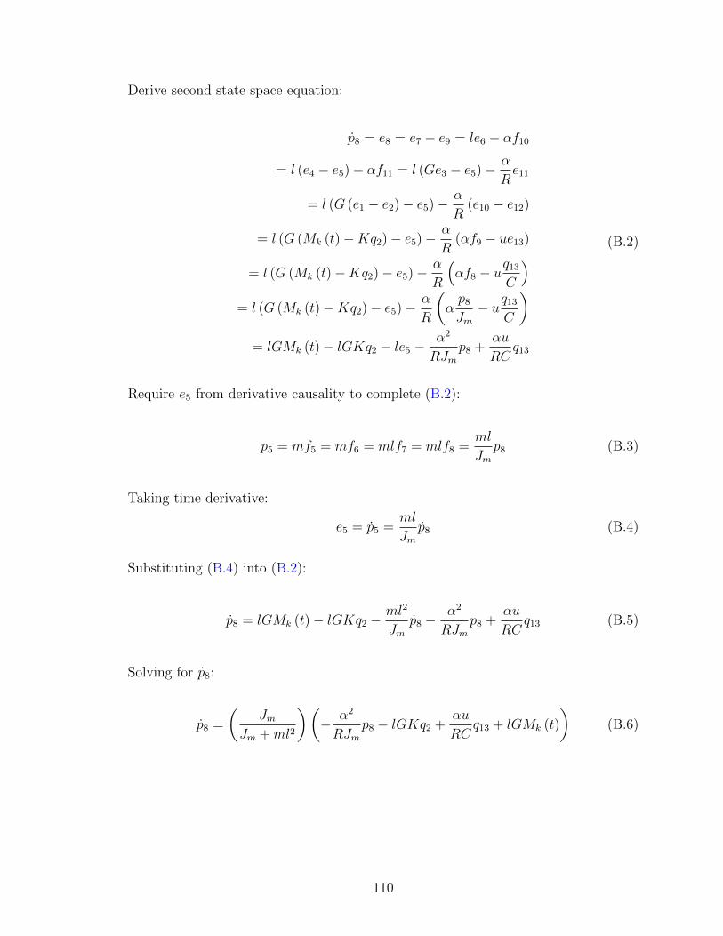
Derive second state space equation:

p8 = e8 = e7 − e9 = le6 − αf10

= l (e4 − e5)− αf11 = l (Ge3 − e5)−α

Re11

= l (G (e1 − e2)− e5)−α

R(e10 − e12)

= l (G (Mk (t)−Kq2)− e5)−α

R(αf9 − ue13)

= l (G (Mk (t)−Kq2)− e5)−α

R

(αf8 − u

q13C

)= l (G (Mk (t)−Kq2)− e5)−

α

R

(αp8Jm− uq13

C

)= lGMk (t)− lGKq2 − le5 −

α2

RJmp8 +

αu

RCq13

(B.2)

Require e5 from derivative causality to complete (B.2):

p5 = mf5 = mf6 = mlf7 = mlf8 =ml

Jmp8 (B.3)

Taking time derivative:

e5 = p5 =ml

Jmp8 (B.4)

Substituting (B.4) into (B.2):

p8 = lGMk (t)− lGKq2 −ml2

Jmp8 −

α2

RJmp8 +

αu

RCq13 (B.5)

Solving for p8:

p8 =

(Jm

Jm +ml2

)(− α2

RJmp8 − lGKq2 +

αu

RCq13 + lGMk (t)

)(B.6)

110

Derive third state space equation:

q13 = f13 = uf12 = uf11 =u

Re11 =

u

R(e10 − e12) =

u

R(αf9 − ue13)

=u

R

(αf8 − u

q13C

)=u

R

(αp8Jm− uq13

C

)= − u2

RCq13 +

αu

RJmp8

(B.7)

Change of variables:

q2 = φk, knee angle

p8 = Jmθm, motor momentum

q13 = qC , capacitor charge

Taking time derivatives:

q2 = φk, knee angular velocity

p8 = Jmθm, motor inertial force

q13 = qC = iC , capacitor current

Substitute change of variables and simplify to form final set of equations:

φk = Glθm (B.8)

θm =1

Jm +ml2

(−α

2

Rθm − lGKφk +

αu

RCqC + lGMk (t)

)(B.9)

iC = − u2

RCqC +

αu

Rθm (B.10)

111

APPENDIX C

Basic Model u-Inversion

An open-loop control method (Section 3.2) was selected for the actuator

simulations. This required the computation of the control variable u from known

information, an application of the method from [35]. The associated process is given

here for the basic actuator model, which is presented as an example case.

Starting from the system equations:

φk = Glθm (C.1)

θm =1

Jm +ml2

(lGMk (t)− lGKφk −

α2

Rθm +

αu

RCqC

)(C.2)

iC =αu

Rθm −

u2

RCqC (C.3)

Multiply (C.3) by qC :

qCiC =αu

RqC θm −

u2

RCq2C (C.4)

Integrate (C.4) with respect to time:

t∫0

qCiCdτ =

t∫0

(αu

RqC θm −

u2

RCq2C

)dτ (C.5)

112

Perform change of variables, qC = x3, iC = x3:

t∫0

x3x3dτ = − 1

RC

t∫0

(ux3)2 dτ +

α

R

t∫0

(ux3) θmdτ (C.6)

Continue integration:

1

2

(x3 (t)2 − x3 (0)2

)= − 1

RC

t∫0

(ux3)2 dτ +

α

R

t∫0

(ux3) θmdτ (C.7)

Solve for x3 (t):

x3 (t)2 = 2

− 1

RC

t∫0

(ux3)2 dτ +

α

R

t∫0

(ux3) θmdτ

+ x3 (0)2 (C.8)

Solve (C.2) for ux3, where x3 = qC :

ux3 =RC

α

((Jm +ml2

)θm − lGMk (t) + lGKφk +

α2

Rθm

)(C.9)

Substitution of (C.9) into (C.8) gives an expression for x3 (t)2 in terms of values that

are either known or could be obtained from reference data. Taking the square root of

this result provides an expression for x3 (t). Finally, dividing (C.9) by this expression

for x3 (t) yields a direct solution for u. The implementation of these final steps can

be completed numerically within MATLAB and are, therefore, not shown here.

113

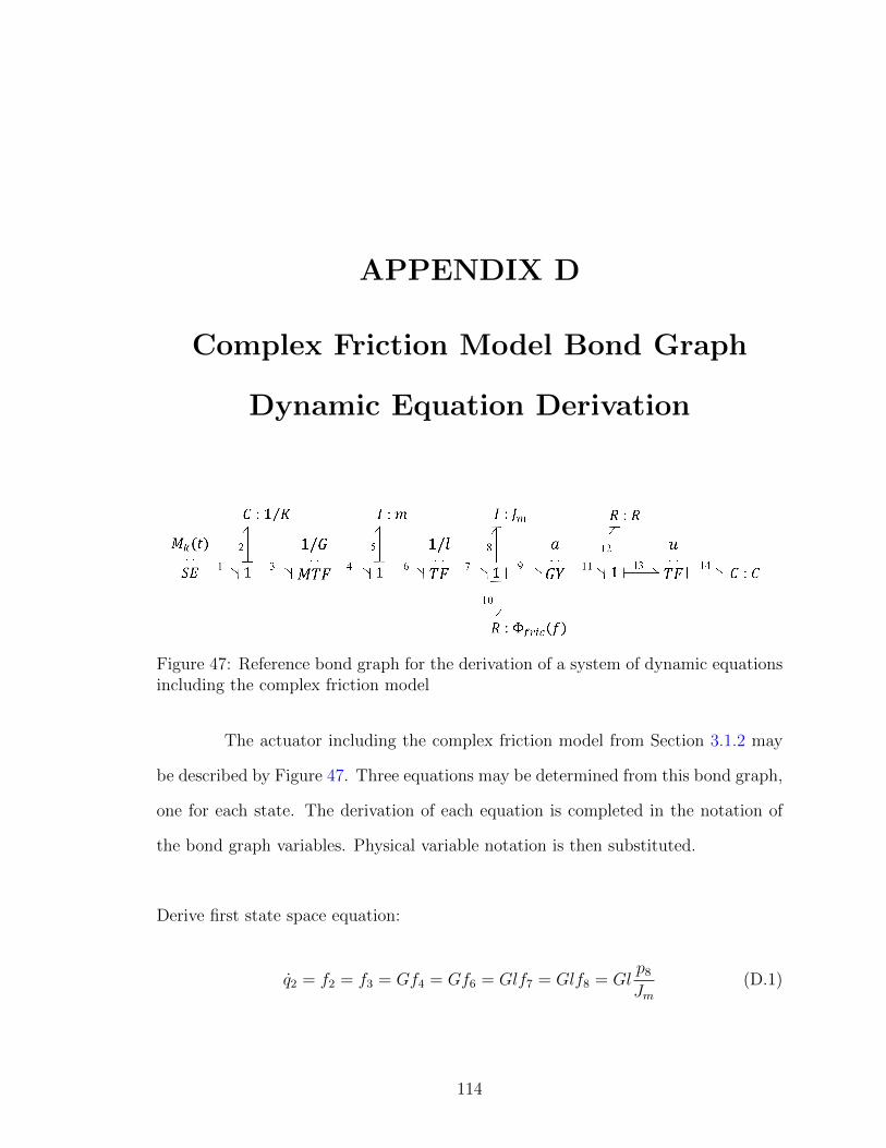
APPENDIX D

Complex Friction Model Bond Graph

Dynamic Equation Derivation

Figure 47: Reference bond graph for the derivation of a system of dynamic equationsincluding the complex friction model

The actuator including the complex friction model from Section 3.1.2 may

be described by Figure 47. Three equations may be determined from this bond graph,

one for each state. The derivation of each equation is completed in the notation of

the bond graph variables. Physical variable notation is then substituted.

Derive first state space equation:

q2 = f2 = f3 = Gf4 = Gf6 = Glf7 = Glf8 = Glp8Jm

(D.1)

114

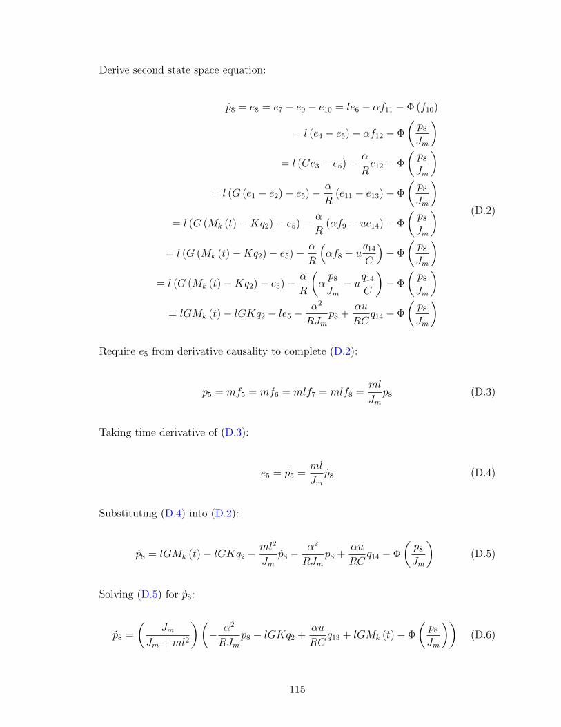
Derive second state space equation:

p8 = e8 = e7 − e9 − e10 = le6 − αf11 − Φ (f10)

= l (e4 − e5)− αf12 − Φ

(p8Jm

)= l (Ge3 − e5)−

α

Re12 − Φ

(p8Jm

)= l (G (e1 − e2)− e5)−

α

R(e11 − e13)− Φ

(p8Jm

)= l (G (Mk (t)−Kq2)− e5)−

α

R(αf9 − ue14)− Φ

(p8Jm

)= l (G (Mk (t)−Kq2)− e5)−

α

R

(αf8 − u

q14C

)− Φ

(p8Jm

)= l (G (Mk (t)−Kq2)− e5)−

α

R

(αp8Jm− uq14

C

)− Φ

(p8Jm

)= lGMk (t)− lGKq2 − le5 −

α2

RJmp8 +

αu

RCq14 − Φ

(p8Jm

)

(D.2)

Require e5 from derivative causality to complete (D.2):

p5 = mf5 = mf6 = mlf7 = mlf8 =ml

Jmp8 (D.3)

Taking time derivative of (D.3):

e5 = p5 =ml

Jmp8 (D.4)

Substituting (D.4) into (D.2):

p8 = lGMk (t)− lGKq2 −ml2

Jmp8 −

α2

RJmp8 +

αu

RCq14 − Φ

(p8Jm

)(D.5)

Solving (D.5) for p8:

p8 =

(Jm

Jm +ml2

)(− α2

RJmp8 − lGKq2 +

αu

RCq13 + lGMk (t)− Φ

(p8Jm

))(D.6)

115

Derive third state space equation:

q14 = f14 = uf13 = uf12 =u

Re12 =

u

R(e11 − e13) =

u

R(αf9 − ue14)

=u

R

(αf8 − u

q14C

)=u

R

(αp8Jm− uq14

C

)= − u2

RCq14 +

αu

RJmp8

(D.7)

Change of variables:

q2 = φk, knee angle

p8 = Jmθm, motor momentum

q14 = qC , capacitor charge

Taking time derivatives:

q2 = φk, knee angular velocity

p8 = Jmθm, motor inertial force

q14 = qC = iC , capacitor current

Substitute change of variables and simplify to form final set of equations:

φk = Glθm (D.8)

θm =1

Jm +ml2

(−α

2

Rθm − lGKφk +

αu

RCqC + lGMk (t)− Φ

(θm

))(D.9)

iC = − u2

RCqC +

αu

Rθm (D.10)

116

APPENDIX E

Generalized Friction Model Bond Graph

Dynamic Equation Derivation

Figure 48: Reference bond graph for the derivation of a system of dynamic equationsincluding the generalized friction model

The system of three equations describing the actuator including the general-

ized friction model for use in optimization from Section 3.1.2 may be determined from

the bond graph in Figure 48. The derivation of each equation is completed in the

notation of the bond graph variables. Physical variable notation is then substituted.

Derive first state space equation:

q2 = f2 = f3 = Gf4 = Gf6 = Glf7 = Glf8 = Glp8Jm

(E.1)

117

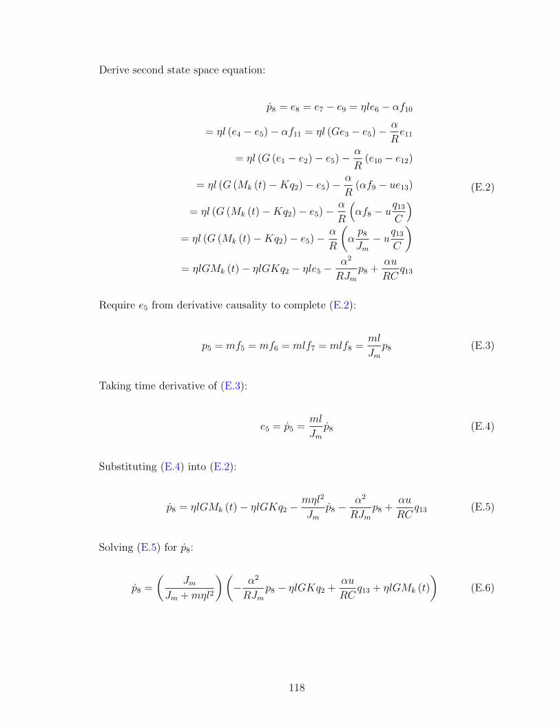
Derive second state space equation:

p8 = e8 = e7 − e9 = ηle6 − αf10

= ηl (e4 − e5)− αf11 = ηl (Ge3 − e5)−α

Re11

= ηl (G (e1 − e2)− e5)−α

R(e10 − e12)

= ηl (G (Mk (t)−Kq2)− e5)−α

R(αf9 − ue13)

= ηl (G (Mk (t)−Kq2)− e5)−α

R

(αf8 − u

q13C

)= ηl (G (Mk (t)−Kq2)− e5)−

α

R

(αp8Jm− uq13

C

)= ηlGMk (t)− ηlGKq2 − ηle5 −

α2

RJmp8 +

αu

RCq13

(E.2)

Require e5 from derivative causality to complete (E.2):

p5 = mf5 = mf6 = mlf7 = mlf8 =ml

Jmp8 (E.3)

Taking time derivative of (E.3):

e5 = p5 =ml

Jmp8 (E.4)

Substituting (E.4) into (E.2):

p8 = ηlGMk (t)− ηlGKq2 −mηl2

Jmp8 −

α2

RJmp8 +

αu

RCq13 (E.5)

Solving (E.5) for p8:

p8 =

(Jm

Jm +mηl2

)(− α2

RJmp8 − ηlGKq2 +

αu

RCq13 + ηlGMk (t)

)(E.6)

118

Derive third state space equation:

q13 = f13 = uf12 = uf11 =u

Re11 =

u

R(e10 − e12) =

u

R(αf9 − ue13)

=u

R

(αf8 − u

q13C

)=u

R

(αp8Jm− uq13

C

)= − u2

RCq13 +

αu

RJmp8

(E.7)

Change of variables:

q2 = φk, knee angle

p8 = Jmθm, motor momentum

q13 = qC = iC , capacitor charge

Taking time derivatives:

q2 = φk, knee angular velocity

p8 = Jmθm, motor inertial force

q13 = qC , capacitor current

Substitute change of variables and simplify to form final set of equations:

φk = Glθm (E.8)

θm =1

Jm +mηl2

(−α

2

Rθm − ηlGKφk +

αu

RCqC + ηlGMk (t)

)(E.9)

iC = − u2

RCqC +

αu

Rθm (E.10)

119

APPENDIX F

Ballscrew Datasheet

Identification of a ballscrew was required for the completion of the complex

friction model of Section 3.1.2. The complete parameters of the selected ballscrew

may be found in the attached datasheet. Of particular interest were the ball circle

diameter, lead, maximum load, and preload capacity.

120

121

APPENDIX G

Updating the crank-slider modulus G

within the energy balance software for the

basic actuator model

Within the simulation of the basic actuator (Section 3.3.1) the initial value

of the G modulus is required, G0. It is used to calculate the initial condition of the

integrator block outputting the motor velocity θm. The value G0 is obtained within

the basic actuator model Simulink by selecting the first value of the bbo.ref.G array.

This array is pre-calculated during the u-inversion process and simply used within

the Simulink. For optimization this approach is suitable and sufficient. However,

the energy balance software is setup to be run after the optimization is complete,

loading the best solution from a .mat file. Prior to the creation of this file, bbo.ref.G

is not updated to reflect the best solution; rather, it contains the G values of the last

evaluated solution candidate. Accordingly, when running the Simulink in its original

form, the value of G0 does not match the best solution case. A method has been

developed to address this oversight:

1. Load .mat file of interest and run Simulink.

2. Get G sim(1) after simulation is complete.

122

3. Replace bbo.ref.G(1) in textbox of bbo.ref.G 0 constant block with G sim(1)

value.

4. Run Simulink again.

5. Run the energy balance code with the workspace resulting from the previous

step still loaded.

For all consecutive models, namely the complex friction and efficiency models, of the

crank-slider actuator this issue has been addressed within the code.

123

APPENDIX H

Heel and Toe Jacobians

To determine the external forces applied to the hip robot and prosthesis

model as referenced in Section 5.1, the linear velocity Jacobians must be computed.

This is completed by taking the time derivatives of the foot kinematic model equations

given in Section 2.2.5 and arranging the results in matrix form. This process must

be completed for each contact point, the heel and the toe, giving Jv,h and Jv,t.

Jv,h(1, 1) = 0

Jv,h(1, 2) = −l2 sin(q2)− l3 sin(q2 + q3)− aH sin

(q2 + q3 + q4 +

(π

2+ cos−1

(ah

aH

)))Jv,h(1, 3) = −l3 sin(q2 + q3)− aH sin

(q2 + q3 + q4 +

(π

2+ cos−1

(ah

aH

)))Jv,h(1, 4) = −aH sin

(q2 + q3 + q4 +

(π

2+ cos−1

(ah

aH

)))Jv,h(2, 1) = 1

Jv,h(2, 2) = l2 cos(q2) + l3 cos(q2 + q3) + aH cos

(q2 + q3 + q4 +

(π

2+ cos−1

(ah

aH

)))Jv,h(2, 3) = l3 cos(q2 + q3) + aH cos

(q2 + q3 + q4 +

(π

2+ cos−1

(ah

aH

)))Jv,h(2, 4) = aH cos

(q2 + q3 + q4 +

(π

2+ cos−1

(ah

aH

)))

124

Jv,t(1, 1) = 0

Jv,t(1, 2) = −l2 sin(q2)− l3 sin(q2 + q3)− aT sin

(q2 + q3 + q4 +

(π

2− cos−1

(ah

aT

)))Jv,t(1, 3) = −l3 sin(q2 + q3)− aT sin

(q2 + q3 + q4 +

(π

2− cos−1

(ah

aT

)))Jv,t(1, 4) = −aT sin

(q2 + q3 + q4 +

(π

2− cos−1

(ah

aT

)))Jv,t(2, 1) = 1

Jv,t(2, 2) = l2 cos(q2) + l3 cos(q2 + q3) + aT cos

(q2 + q3 + q4 +

(π

2− cos−1

(ah

aT

)))Jv,t(2, 3) = l3 cos(q2 + q3) + aT cos

(q2 + q3 + q4 +

(π

2− cos−1

(ah

aT

)))Jv,t(2, 4) = aT cos

(q2 + q3 + q4 +

(π

2− cos−1

(ah

aT

)))

125

APPENDIX I

Hip Robot and Prosthesis Dynamic

Equations

The hip robot and prosthesis dynamic system model referred to in Section 5.1

is provided below. It is written in terms of the parameters Θ, which are given at the

end of the equation set. M is the mass matrix. C is the Coriolis matrix. G is the

gravity vector. And R is the loss terms vector.

M(1, 1) = Θ1

M(1, 2) = Θ2 cos(q2) + Θ3 cos(q2 + q3 + q4) + Θ4 cos(q2 + q3)

M(1, 3) = Θ3 cos(q2 + q3 + q4) + Θ4 cos(q2 + q3)

M(1, 4) = Θ3 cos(q2 + q3 + q4)

M(2, 1) = M(1, 2)

M(2, 2) = Θ5 + 2Θ6 cos(q3 + q4) + 2Θ7 cos(q3) + 2Θ8 cos(q4)

M(2, 3) = Θ9 + Θ7 cos(q3) + 2Θ8 cos(q4) + Θ6 cos(q3 + q4)

M(2, 4) = Θ10 + Θ6 cos(q3 + q4) + Θ8 cos(q4)

126

M(3, 1) = M(1, 3)

M(3, 2) = M(2, 3)

M(3, 3) = Θ9 + 2Θ8 cos(q4) +m4l23 + I3z + I4z

M(3, 4) = Θ10 + Θ8 cos(q4)

M(4, 1) = M(1, 4)

M(4, 2) = M(2, 4)

M(4, 3) = M(3, 4)

M(4, 4) = Θ10

C(1, 1) = 0

C(1, 2) = −q3(Θ3 sin(q2 + q3 + q4) + Θ4 sin(q2 + q3))

− q2(Θ2 sin(q2) + Θ3 sin(q2 + q3 + q4) + Θ4 sin(q2 + q3))

−Θ3q4 sin(q2 + q3 + q4)

C(1, 3) = −q2(Θ3 sin(q2 + q3 + q4) + Θ4 sin(q2 + q3))

− q3(Θ3 sin(q2 + q3 + q4) + Θ4 sin(q2 + q3))−Θ3q4 sin(q2 + q3 + q4)

C(1, 4) = −Θ3q2 sin(q2 + q3 + q4)−Θ3q3 sin(q2 + q3 + q4)−Θ3q4 sin(q2 + q3 + q4)

C(2, 1) = 0

C(2, 2) = −q3(Θ6 sin(q3 + q4) + Θ7 sin(q3))− q4(Θ6 sin(q3 + q4) + Θ8 sin(q4))

C(2, 3) = −q2(Θ6 sin(q3 + q4) + Θ7 sin(q3))− q3(Θ6 sin(q3 + q4) + Θ7 sin(q3))

− q4(Θ6 sin(q3 + q4) + Θ8 sin(q4))

C(2, 4) = −q2(Θ6 sin(q3 + q4) + Θ8 sin(q4))− q3(Θ6 sin(q3 + q4) + Θ8 sin(q4))

− q4(Θ6 sin(q3 + q4) + Θ8 sin(q4))

127

C(3, 1) = 0

C(3, 2) = q2(Θ6 sin(q3 + q4) + Θ7 sin(q3))−Θ8q4 sin(q4)

C(3, 3) = −Θ8q4 sin(q4)

C(3, 4) = −Θ8q2 sin(q4)−Θ8q3 sin(q4)−Θ8q4 sin(q4)

C(4, 1) = 0

C(4, 2) = q2(Θ6 sin(q3 + q4) + Θ8 sin(q4)) + Θ8q3 sin(q4)

C(4, 3) = Θ8q2 sin(q4) + Θ8q3 sin(q4)

C(4, 4) = 0

G(1) = −gΘ1

G(2) = −g(Θ2 cos(q2) + Θ3 cos(q2 + q3 + q4) + Θ4 cos(q2 + q3))

G(3) = −gΘ4 cos(q2 + q3)− gΘ3 cos(q2 + q3 + q4)

G(4) = −gΘ3 cos(q2 + q3 + q4)

R(1) = Θ12sign(q1)

R(2) = Θ11q2

R(3) = 0

R(4) = 0

128

Θ1 = m1 +m2 +m3 +m4

Θ2 = c2m2 + l2m3 + l2m4

Θ3 = c4m4

Θ4 = c3m3 + l3m4

Θ5 = I2z + I3z + I4z + c22m2 + c23m3 + c24m4 + l22m3 + l22m4 + l23m4

Θ6 = c4l2m4

Θ7 = c3l2m3 + l2l3m4

Θ8 = c4l3m4

Θ9 = m3c23 +m4c

24 +m4l

23 + I3z + I4z

Θ10 = I4z + c24m4

Θ11 = b

Θ12 = f

129

APPENDIX J

Optimized Switched Robust

Tracking/Impedance Controller Gains

A total of 50 control gains were optimized as described in Section 5.5. This

appendix details a portion of the results of that optimization, Section 5.6. The

selected values for each of the 50 gains were tabulated and categorized by state for a

total of five optimization trials.

130

State Gain Trial 1 Trial 2 Trial 3 Trial 4 Trial 5

State 0

Λ3 2104.55 2072.13 1074.12 2897.02 3887.34K3 3510.48 339.96 635.97 3600.80 3627.69I3 0.60 0.44 5.49 3.99 3.30b3 2859.94 5041.61 2975.51 2212.36 1559.57k3 46428.67 55453.93 42016.98 36983.24 24394.90Λ4 1289.75 2711.00 953.03 2786.35 2603.17K4 2760.94 3884.77 3350.25 1124.62 990.47I4 3.08 1.34 0.92 2.04 5.75b4 201.52 289.06 1353.91 2976.18 1195.37k4 662.00 51525.59 57692.63 6193.19 63314.20

State 1

Λ3 840.20 1180.68 847.62 2608.33 895.00K3 1642.72 249.16 2388.50 3012.43 2293.19I3 5.05 3.63 1.13 2.73 2.48b3 476.70 507.42 264.99 190.86 3431.62k3 5517.38 8505.50 7792.28 2529.88 8554.47Λ4 411.44 1484.58 1799.74 3528.20 2487.95K4 2349.47 3086.26 853.52 3939.37 467.45I4 5.52 3.72 4.75 1.07 2.51b4 1240.47 2994.85 2640.80 522.91 2245.83k4 3715.36 3848.21 4190.58 74395.32 1903.05

State 2

Λ3 3926.98 1314.79 935.32 1578.02 44.21K3 283.15 999.83 1309.65 2286.33 3958.97I3 1.13 0.63 0.55 4.15 1.88b3 4009.22 1712.07 613.32 4104.68 3074.07k3 19596.31 20026.24 64006.87 58063.54 66237.25Λ4 37.17 810.28 248.95 2782.64 728.87K4 3389.48 447.92 987.10 239.33 889.69I4 2.36 1.55 1.33 3.65 2.75b4 1588.69 1494.52 1933.04 548.65 2036.18k4 42832.44 41845.03 47102.95 68449.88 34863.64

State 3

Λ3 695.70 488.79 1261.56 1062.97 1677.96K3 3911.88 2989.00 1206.15 1052.94 3860.55I3 1.90 2.36 2.10 0.70 2.89b3 1267.55 1043.15 3530.01 500.00 707.29k3 38853.24 3000.00 51825.81 68264.84 24772.57Λ4 3477.74 2961.47 495.94 3868.01 278.95K4 671.86 2503.44 1390.67 824.59 1338.31I4 3.32 1.35 3.87 3.17 1.89b4 2741.74 1354.73 1306.85 2865.91 1453.44k4 58165.57 47725.56 49530.21 61164.89 19111.19

State 4

Λ3 1294.74 2431.33 1499.49 1153.22 2967.92K3 816.46 2962.23 2162.88 1960.42 167.88I3 1.00 1.23 2.97 2.09 0.95b3 150.00 4903.62 3037.19 772.85 2137.13k3 55066.01 72544.84 69714.07 72281.89 53811.24Λ4 3540.41 994.05 329.88 2417.60 3032.79K4 310.32 757.90 2741.41 550.00 3572.16I4 2.07 1.17 5.71 3.00 1.63b4 2195.18 1245.47 1350.52 1110.14 2538.19k4 59146.21 13357.86 73791.00 48473.00 69428.06

Table XVII: Control gains resulting from five optimization trials131

APPENDIX K

Code Repository

Each of the code suites developed for the contributions of this work are available at

the following URL’s:

Chapter III: Actuator System Design and Optimization

http://embeddedlab.csuohio.edu/Prosthetics/CrankSliderActuator.html

Chapter IV: Ground Contact Model Design and Optimization

http://embeddedlab.csuohio.edu/Prosthetics/GroundContactModel.html

Chapter V: Control System Design and Optimization

http://embeddedlab.csuohio.edu/Prosthetics/SwitchedRobTrackImpCont.html

132

APPENDIX L

Copyright Permissions

Several figures as denoted throughout this work were adapted from previous

publications of other authors. All were used with permission. For Figures 1 and 2

this permission was granted through an automated system. This process is shown in

the first three images. Permission for Figure 6 was granted in writing, which is the

final image. The incorporation of Figure 39 into this work was completed according

to the IEEE guidelines.

133

Permission granted for use of C-leg and Mauch SNS kinematics plots of Figure 1 from[38]

134

Type of permission requested for use of joint power plots of Figure 2 from [25]

135

Permission granted for use of joint power plots of Figure 2 from [25]

136

Permission granted for use and adaptation of coordinate system illustration of Figure 6from [37]

137