optimization of a chilled water plant without storage ... · optimization of a chilled water plant...

Optimization of a chilled water plant without storage using a forward plant model

Zhiqin Zhanga, PhD William D. Turnera, PhD, PE Qiang Chena, PE Chen Xub, PE Song Denga, PE aEnergy Systems Laboratory bVisionBEE

Texas A&M University 3112 Windsor Road A 124 College station, Texas, USA Austin, Texas, USA

ABSTRACT This paper introduces a forward chilled water

plant model to optimize the setpoints of continuous controlled variables in a chiller plant without storage and controlled by supervisory control. It can also be used to estimate the savings potential of some energy conservation measures. This model is based on a Wire-to-Water efficiency concept to simulate the plant power for producing cooling. The fluctuation of the chilled water loop supply and return temperature difference is also considered to reflect its effects on the chiller loading and pumping power. The variables to be optimized could be cooling tower approach, chiller chilled water leaving temperature, and chiller condenser water flow rate. This is a non-linear programming problem and can be solved with the generalized reduced gradient nonlinear solver. The application of this model is illustrated with a practical chilled water system.

INTRODUCTION A chiller plant produces chilled water (ChW)

and transports it to end users, such as air handling units, through piping. Ever since 1990, traditional ChW plant design has begun utilizing a primary-secondary loop configuration. The imbalance in flow between the primary and secondary circuits results in flow through the bypass piping circuit. The appearance of variable primary flow in 1996 made the bypass line unnecessary. But another bypass line may be designed at loop end to make sure the chiller minimum flow rate is guaranteed (Durkin 2005). This study will focus on a primary-secondary loop configuration.

The energy performance of most existing ChW

plants is not very efficient. It was estimated that about 90% of water-cooled, centrifugal, central plants operated in the 1.0-1.2 kW per ton “needs improvement” range, while a highly efficient plant can reach 0.75 kW per ton (Erpelding 2006). All

kinds of problems are to blame, such as the low delta-T syndrome (Kirsner 1995), low part load ratio (PLR), significant mixing, valve and pump hunting, higher than needed pump pressure, etc. In addition, there are other reasons for plant optimization, such as equipment performance degrading with age, load changes (Taylor 2006), plant expansion in an unorganized manner, and energy cost fluctuations. Therefore, enhancing the performance of cooling plants is an urgent and important task.

Automatic control systems have been widely

applied in chiller plants to achieve robust, effective, and efficient operation of the system on the basis of ensuring thermal comfort of occupants and satisfying indoor air quality. Generally, all the control methods used in heating, ventilating, and air conditioning (HVAC) systems can be divided into supervisory control and relational control. Supervisory control, often named optimal control, seeks stable and efficient operation by systematically choosing properly controlled variables setpoints, such as flow, pressure or temperature. These setpoints can be reset when uncontrolled variables (such as ambient air wet bulb (WB), dry bulb (DB) temperature, and building cooling load) are changed, and they are maintained by modulating control variables (speed of components) through proportional integral derivative (PID) controllers or sequencing. This method is easy to understand and implement in practice. Relational control is to determine continuous and discrete control variables directly according to uncontrollable variables or equipment power input, such as demand-based control (Hartman 2001b) and load-based control (Yu and Chan 2008). It was claimed by the authors that these controls could realize tremendous energy savings.

The fundamentals of supervisory control

strategies have been comprehensively introduced in the ASHRAE Handbook (2003b) and are widely applied in practice. Most of these controls originated from the supervisory control methodology developed by J. E. Braun (1988). Based on model-based

ESL-IC-10-10-20

Proceedings of the Tenth International Conference for Enhanced Building Operations, Kuwait, October 26-28, 2010

simulation, the optimal setpoint reset and equipment sequencing can be related to uncontrollable variables. The parameter estimate methods and implementation algorithms are also presented. These general optimal or near-optimal control guidelines for a typical chiller plant are widely accepted due to their simplicity and effectiveness.

In general, chiller plant optimization can be

divided into static optimization and dynamic optimization depending on if there is considerable storage system. The optimization related to the systems without storage is a quasi-steady, single-point optimization. The ASHRAE Handbook (ASHRAE 2003b) presents a framework for determining optimal controls and a simplified approach for estimating control laws for cooling plants without storage. General static optimization problems are mathematically stated as the minimization of the sum of the operating costs of each component with respect to all discrete and continuous control variables, subject to equality constraints and inequality constraints. Typical input and output stream variables for thermal systems are those controlled variables, such as flow, pressure, and temperature. Static optimization is applied to all-electric systems without significant storage, leading to minimization of power at each instant in time. Optimization problems of building HVAC systems are often characterized with discretization, nonlinearity, and high constraints. Nonlinear optimization techniques are more powerful and useful and can be divided into local and global optimization.

Some local optimization studies have been

conducted by researchers. Graves (2003) presented a thermodynamic model for a screw chiller and cooling tower system for the purpose of developing an optimized control algorithm for the chiller plant and obtained a 17% reduction in the energy consumption. Lu et al. (2004) presented a model-based optimization strategy for the condenser water (CW) loop of centralized HVAC systems. A modified generic algorithm for this particular problem was proposed to obtain the optimal set points of the process and the operating cost of the condenser water loop could be substantially reduced. Chang et al. (2005) proposed a method for using the branch and bound method to solve the optimal chiller sequencing problem and to eliminate the deficiencies of conventional methods and much power was saved. Furlong and Morrison (2005) studied the optimization of CW system cooling tower (CT) and chiller combination. The conclusions only applied to design conditions. Chang (2006) attempted to solve

the optimal chiller loading problem by utilizing simulated annealing. The case study analysis demonstrates that this method solves the Lagrangian problem and generates highly accurate results. Bahnfleth and Peyer (2006; 2007) investigated the economics of variable primary flow chilled water pump systems via a parametric modeling study. It is found that variable primary flow systems reduced total annual plant energy use by 2-5%, first cost by 4-8%, and life-cycle cost by 3-5%. Yu and Chan (2007) recommended using uneven load sharing strategies for multiple chillers to enhance their aggregate coefficient of performance (COP). It is applicable to chiller plants with air-cooled reciprocating chillers, given that their COP increases with chiller PLRs and approaches the highest level at full load for any given outdoor temperature.

It is easier to study the performance of a

subsystem and the conclusions drawn may provide some insights into the local optimal control. The following researchers tried to find some general optimal control rules on the whole system level: Hackner et al. (1985) and Lau (1985) utilized component models to simulate and search the minimum power consumption for the operation of building HVAC systems. The comparison studies showed that these techniques could save more energy as compared to local optimization methods. Braun (1988) and Braun et al.(1989c) presented a component-based nonlinear optimization and simulation tool and used it to investigate optimal performance. The results showed that optimal set points could be correlated as a linear function of load and ambient WB temperature. Cumali (1988) presented a method for real-time global optimization of HVAC systems including the central plant and associated piping and duct networks. Electrical demand reductions of 8% to 12% and energy savings of 18% to 23% were achieved in practical applications. Olson (1993) presented a dynamic chiller sequencing algorithm for controlling the HVAC equipment necessary to cool non-residential buildings. This is accomplished by forecasting the cooling loads expected through a planning horizon, determining the minimum cost way of meeting the individual loads with various combinations of equipment, and using a modified shortest path algorithm to determine the sequence of equipment selection that will minimize the cost of satisfying the expected loads for the entire planning horizon.

Kota et al. (1996) showed that differential

dynamic programming was more efficient compared with non linear programming for optimal control of building HVAC systems, while non-linear

ESL-IC-10-10-20


programming (NLP) was more robust and could treat constraints on the state variables directly. Lu et al. (2005b) have presented the optimal set point control for the global optimization problem for overall HVAC systems using a modified generic algorithm. The problem was solved to minimize the overall system energy consumption by appropriately setting the operating point of each component. However, it is very difficult to get the sufficiently well-tuned controllers to complete the ideal local control loops. For real-time control applications, Sun and Reddy (2005) suggested using the simple control laws for near-optimal control of HVAC systems. Based on the developed complete simulation-based sequential quadratic programming, optimal control maps could be generated using detailed simulations. The regression model for each control variable can then be developed from the control map of the corresponding control variable and was used for near-optimal control of the operation of HVAC systems.

Sometimes, it takes too much effort to build a

component-based model or the necessary data may not be available. An alternative way is to simulate the plant power with one function. This methodology was first advanced by Braun et al. (1989c) when they developed a system-based optimization based on results from component-based optimization. The method involves correlating overall cooling plant power consumption using a quadratic function form. The inputs are uncontrolled variables and controlled continuous variables while outputs are total cost. Separate cost functions are necessary for each operating mode. Minimizing this function leads to linear control laws for controlled continuous variables in terms of uncontrolled variables. The empirical coefficients of this function depend on the operating modes so that these constants must be determined for each feasible combination of discrete control modes. The determined controlled variables will be maintained by modulating continuous control variables, such as valve open percentage and motor speed.

Braun et al. (1987) correlated the power

consumption of the Dallas-Ft. Worth airport chillers, condenser pumps, and cooling tower fans with the quadratic cost function. In subsequent work, Braun et al. (1989c) considered complete system simulations (cooling plant and air handlers) to evaluate the performance of the quadratic, system-based approach. This methodology has been adopted by Ahn and Mitchell (2001) to find the influence of the controlled variables on the total system and component power consumption. A quadratic linear regression equation for predicting the total cooling

system power in terms of the controlled and uncontrolled variables was developed using simulated data collected under different values of controlled and uncontrolled variables. The trade-off among the components of power consumption resulted in the total system power use in that both simulated and predicted systems were minimized at lower supply air, higher chilled water, and lower condenser water temperature conditions. Bradford (1998) developed linear, neural network, and quadratic type system-based models and a component-based model to predict the system energy consumption including demand side. It has been shown that the use of component-based models for either on-line or off-line optimal control is viable and robust.

Although the system-based plant model is much

simpler than the component-based model, the objective function under each feasible combination of discrete control modes has to be generated, and considerable regression error as well as solution difficulty may exist. The component-based models are more accurate, but it takes a long time to build the model for each project. Iterations are inevitable and convergence could be a problem. Some sophisticated algorithms are also required to optimize such a system.

The objective of this paper is to develop a

farward plant model to simulate and optimize the operation of a chilled water plant without storage. Its application is illustrated with a real system to find the optimal reset schedule of the chiller ChW leaving temperature and CT approach temperature. The energy and billing cost savings potential of several energy conservation measures are also estimated.

METHOD Figure 1 shows the general physical

configuration of a primary-secondary loop ChW system. All the variables shown are setpoints that could be optimized. In practice, these setpoints are maintained by adjusting the equipment speed or control valve position with a PID controller. As mentioned before, except for continuous controlled variables, discrete control variables will also need to be optimized, such as sequencing of chillers, cooling towers, and pumps. The constraints on the equipment operation, such as maximum and minimum flow rates, limit the possible number of combinations of control variables.

Plant Power Modeling The system total power can be divided into plant

power and non-plant power. The electricity

ESL-IC-10-10-20


consumed by chilled water production is considered as plant power while all other electricity consumptions, such as air compressors, lighting, and plug loads, are non-plant power.

Figure 1. Configuration of a primary-secondary loop chilled water system

Figure 2 is a flow chart of the ChW plant power

simulation model. All the variables on the left are the inputs while the output is the plant total power. The plant model determines the plant total power consumptions in response to a set of external parameters and a set of plant parameters. For each given plant total ChW flow rate, the ChW plant model will export the total plant power under the given conditions. In this study, an equipment performance-oriented plant model is proposed to calculate the plant power under predefined conditions. This model is based on a Wire-to-Water (WTW) plant efficiency concept. The WTW efficiency of a pump was first introduced by Bernier and Bourret (1999). It was originally used to quantify the whole performance of a ChW plant. In this study, it is used to define the transportation efficiency of plant equipment except for SPMPs.

The system total power can be calculated from

the following formula: ( ) plant_nonSPMPChW,PlantPPMPCHLRCWPCTsys PPQP +++++= ξξξξ (1)

Some regression formulas together with energy

conservation laws are used to simulate the WTW efficiency of pumps and CTs. This forward plant model can be easily set up and used for plant energy simulation. Since it is based on basic physical definitions and conservation laws, it has an explicit physical meaning. Its application is not restricted by the equipment number and sequencing strategies. All calculations are explicit expressions and no iterations are required. One prerequisite is that the pumps are

well sequenced and controlled such that the pump head and efficiency are around the normal operation point.

The optimization of a chiller plant is to find the

reset schedule of some controlled variables to minimize an objective function, such as the monthly or annual utility billing cost. This is a NLP problem and it can be solved with the generalized reduced gradient (GRG) nonlinear solver. This method and specific implementation have been proven in use over many years as one of the most robust and reliable approaches to solve difficult NLP problems.

PCHLR

ξCHLR

ξCWP

ξCT

ξPPMP

ΔTChW

PPPMP

PPlant

TCHLR,CW,S

QPlant

VCHLR,ChW,per

NCHLR

e

DPLp

VLp,ChW

ηSPMP

SPMP

HPPMP

ηPPMP

PPMP

TCHLR,ChW,S

TCHLR,ChW,R

c0, c1, c2, c3

VCHLR,CW,perCHLR

Twb

ΔTApp,sp

d1, d2

HCWP

ηCWP

QCHLR,per

CT

CWP

ΔTApp

Figure 2. Flow chart of chilled water plant power simulation

Chiller Modeling Because of its high weight and significant

complexity, more effort should be made on chiller performance modeling. In this study, a Gordon-Ng model for vapor compression chillers with variable condenser flow is selected in this study. It can apply to unitary and large chillers operating under steady-state variable condenser flow conditions. This model is strictly applicable to inlet guide vane capacity control (as against cylinder unloading for reciprocating chillers, or VSD for centrifugal chillers) (Jiang and Reddy 2003). It is in the following form:

3322110 xcxcxccy +++= (2)

ESL-IC-10-10-20


ChW

cho

QTx =1

, cdiChW

chocdi

TQTTx −

=2,

cdi

ChW

T

QCOPx

⎟⎠⎞

⎜⎝⎛ +

=11

3

( ) cdi

ChW

pwwper,CWcdi

cho

T

QCOP

cVT

TCOPy

⎟⎠⎞

⎜⎝⎛ +

−−⎟⎠⎞

⎜⎝⎛ +

=11

1111

ρ

( ) 15.2739/532,, +×−= SChWCHLRcho TT ( ) 15.2739/532,, +×−= SCWCHLRcdi TT

412,3000,12 , perCHLR

ChW

QQ = ,

CHLR

ChW

PQCOP = ,

perCWCHLRCW VV ,,0.00006309=

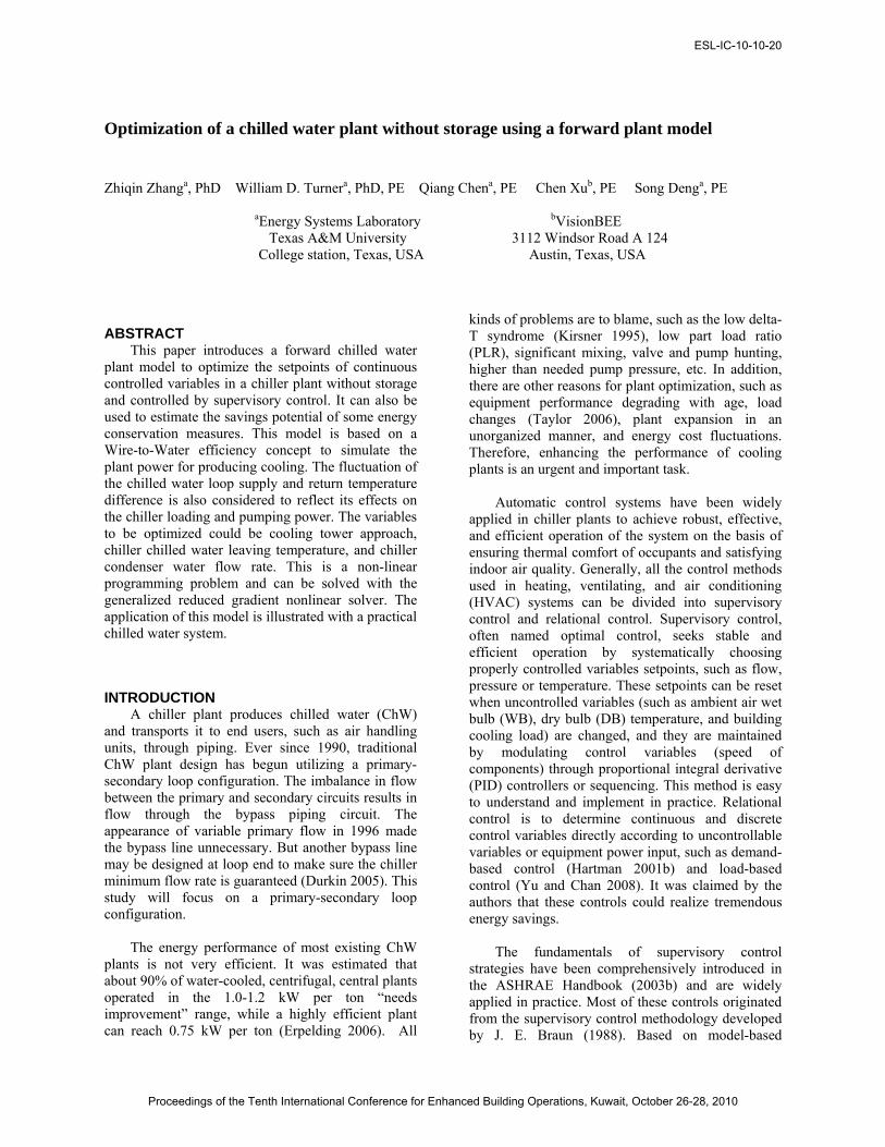
The chiller WTW efficiency (kW per ton) is:

( )

( ) ⎟⎟⎟⎟⎟

⎠

⎞

⎜⎜⎜⎜⎜

⎝

⎛

−−+−

+++== 1

)(

1517.3

000,12412,3

3

22110

pwwCW

ChWchoChW

cdi

ChW

CHLRCHLR

cVQTQc

Txcxcc

Q

P

ρ

ξ

(3)

It is noted that the actual chiller ChW flow is also limited by the upper and lower limits of evaporator ChW flow rate. The upper limit is intended to prevent erosion and the lower limit is to prevent freezing in the tubes.

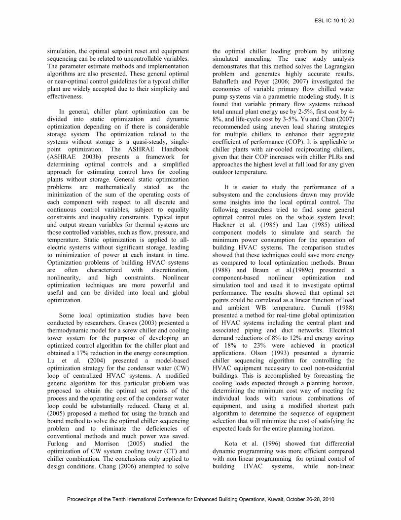
Pump Modeling The general calculation formula of the pump

power is:

allpump ,

HV.Pη9603

7460 ×= (4)

where allη is the overall efficiency including pumps, motors, and VSDs.

The total cooling transported by the pump is:

24

ChWChWChW

TVQ Δ= (5)

The pump WTW efficiency is:

ChWChWallChW

pumppump TV,

HV.QP

Δ×

×==

249603

7460η

ξ (6)

For PPMPs, V = ChWV . The WTW efficiency is:

ChWPPMP

PPMPPPMP T

HΔ

=η

ξ 004521.0 (7)

For CWPs, V =

perCWpump VN ,× . Consequently, the CW pump WTW efficiency is:

per,ChW

per,CW

CWP

CWPCWP Q

VH.η

ξ 00018840= (8)

For SPMPs, the pump power is:

( )

SPMP

ChWLpLpChWLpSPMP

eVDPVP

η960,331.2746.0 2

__ +××= (9)

The head and efficiency of pumps can be

simulated as a function of pump flow rate or be constant. Obviously, the energy consumption of SPMPs is subject to the loop side operation and is not determined by plant operations.

Cooling Tower Modeling The mass and heat transfer process in a cooling

tower is fairly complicated. The effectiveness-NTU model is the most popular model in CT simulations but iterations are required to obtain a converged solution (Braun 1989). To overcome this obstacle, a simple CT fan power model is proposed to calculate the tower WTW performance:

( )CHLRApp

21

ChW

CTCT ξ.1

ΔTdd

QPξ 28430+⎟

⎟⎠

⎞⎜⎜⎝

⎛+== (10)

The actual CT approach temperature is obtained

from the following formula:

wbRCWCTApp TTT −=Δ ,, (11)

The coefficients 1d and 2d are regressed from

the trended data, and AppTΔ is maintained by

sequencing the cooling towers or modulating fan speed.

Loop Delta-T The loop ChW delta-T is subject to many

factors, such as chiller ChW leaving temperature, cooling coil air leaving temperature, type of flow control valves, coil design parameters and degrading due to fouling, tertiary connection types, coil cooling load, air economizers, etc. Considering the difficulties in developing a physical model to simulate the loop delta-T, a linear model regressed from the trended data is used in this study.

01

hxhTn

iiiLp +=Δ ∑

=

(12)

where

ix are the variables that could be the dominant factors of the loop delta-T model, such as ChW supply temperature, loop total cooling load, ambient

ESL-IC-10-10-20


DB and WB temperature, hour of the day, weekday or weekends, and month. The air system side parameters, such as coil air leaving temperature, total air flow rate, coil design delta-T, and sensible load ratio, are not included due to the diversity or unpredictability.

The exact form of the regression model may vary for different projects. It could be necessary to build different models to accommodate air-conditioning system operation changes at different seasons. A constant delta-T can be used in a rough, first order simulation.

APPLICATION

System Description The system investigated in this study is a central

utility plant called Energy Plaza (EP) located in the Dallas-Fort Worth metropolitan area. The EP consists of six 5500 ton(19,343kW)constant-speed centrifugal chillers, called on-site manufactured (OM) chillers, one 90,000 ton-hr naturally stratified ChW storage tank, six 150 hp constant speed primary pumps, four 450 hp variable-speed secondary pumps, eight 400 hp CW pump, and eight 150 hp two-speed cooling towers. Figure 3 shows a schematic diagram of this chilled water system. This study only deals with the ChW system operated without thermal storage.

Figure 3. Schematic diagram of the EP ChW system The monthly electricity billing cost consists of a

meter charge, current month non-coincident peak (NCP) demand charge, four coincident peak (4CP) demand charge, and energy consumption charge. The total monthly electricity billing charge ( TotalC ) is:

nconsumptioenergyNCPNCPCPCPpodeliveryTotal ERDRDRCC +++= 44int_

(13) The rates CPR4 , NCPR , and

energyR for each month are subject to minor adjustments, and the rates from selected one year period are used in the simulation. The meter charge

int_ podeliveryC is constant for each month. All demand kWs used have been adjusted to 95% power factor. The monthly average power

factors during this period will be used in the power factor correction.

The 4CP demand kW is the average of the

plant’s integrated 15 minute demands at the time of the monthly Electric Reliability Council of Texas (ERCOT) system 15 minute peak demand for the months of June, July, August and September (called summer months) of the previous calendar year. The exact time will be announced by ERCOT. The plant’s average 4CP demand will be updated effective on January 1 of each calendar year and remain fixed throughout the calendar year. The NCP kW applicable shall be the kW supplied during the 15 minute period of maximum use during the billing month. The current month NCP demand kW shall be the higher of the NCP kW for the current billing month or 80% of the highest monthly NCP kW established in the eleven months preceding the current billing month.

The ChW flow through the chiller evaporator is

controlled by modulating flow control valves on the leaving side of the evaporator. The sequencing of the constant speed primary pumps (PPMPs) is dedicated to the corresponding chillers. The varaible-frequency device (VFD) speed of the secondary pumps (SPMPs) is modulated to maintain the average of differential pressures at the loop ends in the tunnels at a given setpoint. This setpoint is manually adjusted to be between 25 psid (172 kPa) and 48 psid (331 kPa) all year round to ensure there are no hot complaints from terminals. The cooling tower staging control in place is to stage the number of fans and select high and low speed of fans to minimize the chiller compressor plus CT fan electricity consumption.

System Modeling System power. The trended historical data are

used for system modeling. The electricity consumed by OM chillers, CT fans, CW pumps, PPMPs and SPMPs is considered as plant chilled water electricity load while all other electricity consumptions, such as EP air-conditioning, air compressors, lighting, and plug loads, are non-plant electricity loads.

To check the accuracy of the system model, the

EP monthly utility bills are compared with the simulation results. A good match is found although minor differences exist in several months. This could be attributed to imperfection of models, inaccurate parameter inputs, or operations different from actual situations. The present system power model can reasonably predict the monthly electricity consumption.

ESL-IC-10-10-20


Table 1. Parameters of TES system loop side

LP end DP upper setpoint DPh 28.0 psid LP end DP lower setpoint DPl 22.0 psid LP end DP upper shift flow Vupper 16,000 GPM LP end DP lower shift flow Vlower 10,000 GPM LP hydraulic coef.1 e1 1.00E-07 LP hydraulic coef.2 e2 5.00E-08

Loop Hydraulic

LP hydraulic coef.3 e3 3.00E-08 LP supply temperature rise ΔTs 1.0 ºF LP DT coef.0 h0 32.1898 LP DT coef.1 (TLP,ChW,S) h1 -0.5439 LP DT coef.2 (QLP,ChW) h2 6.86E-05 LP DT coef.3 (Twb) h3 6.34E-02 LP max DT ΔTLp,max 22.0 ºF

Loop DT

LP min DT ΔTLp,min 12.0 ºF Loop side modeling. The parameters and inputs

for the TES system loop side are shown in Table 1. The upper and lower limits of the loop end DP as well as the loop flow rate change points are subject to hydraulic requirements and operating experiences. If the loop total ChW flow rate is equal to or lower than 10,000 gallon per minute (GPM) (0.63m3/s), the differential pressure (DP) setpoint is 22.0 psid (151 kPa). If the rate is equal to or higher than 16,000 GPM(1.01m3/s), the DP setpoint is 28.0 psid (193 kPa). The ChW secondary DP setpoint be reset linearly from 22 psi to 28 psi, when the secondary ChW flow is between 10,000 GPM (0.63m3/s) and 16,000 GPM (1.01m3/s). A loop load factor is defined to test the savings when the actual load profile is different from the one used in the simulation.

A temperature rise exists between the loop

supply temperature and the chiller ChW leaving temperature, which is due to pumping heat gain and piping heat losses. The trended data show that the temperature rise fluctuates between 0.0ºF (0.0ºC)and 2.0ºF (1.1ºC) most of time and the annual average temperature rise is 1.0 ºF (0.6ºC).

When the tunnel end DP setpoints are

determined, a loop hydraulic coefficient is required to calculate the differential pressure before and after the SPMPs. Three hydraulic coefficients are regressed from trended data corresponding to one, two, or three SPMPs running scenarios. The coefficients can be regressed from a plot of tunnel piping DP losses versus tunnel total flow rate.

Equation (14) is a linear regression model developed to simulate the loop delta-T as a function of ChW loop supply temperature (x1), loop total cooling load (x2), and ambient WB temperature (x3). A higher loop supply temperature, a lower WB temperature, and a lower loop total ChW load lead to a lower loop delta-T, which is consistent with the observations. An upper and a lower limit are defined to avoid unreasonable regression results when an extrapolation is applied. The system error of the loop delta-T can be used to check the effect of loop delta-T prediction deviations on the system total energy and costs.

3322110 xhxhxhhTLp +++=Δ (14)

8.0

10.0

12.0

14.0

16.0

18.0

20.0

22.0

8 10 12 14 16 18 20 22

Measured delta-T (ºF)

Pre

dict

ed d

elta

-T (º

F)

Figure 4. Comparison of measured and predicted loop delta-Ts

Figure 4 is a comparison of the measured and

predicted ChW supply and return temperatures. If the model accurately fits the data on which it was trained, this type of evaluation is referred to as

ESL-IC-10-10-20


Table 2. Parameters of ChW system plant side

SPMP overall efficiency ηspmp 75% SPMP

SPMP design flow rate Vspmp 8,000 GPM PPMP overall efficiency ηppmp From curves

PPMP PPMP head Hppmp From curves ft CHLR Coefficient 0 c0 -2.81E-01 CHLR Coefficient 1 c1 1.02E+01 CHLR Coefficient 2 c2 1.74E+03 CHLR Coefficient 3 c3 2.71E-03 CHLR Cond. water flow Vcw 10,300 GPM ChW leaving temperature TChW,S 36 ºF CHLR ChW low limit Vchw,min 4,000 GPM CHLR ChW high limit Vchw,max 7,400 GPM Motor max power input Pmtr,max 3,933 kW Max CW enter temp TCW,max 83.0 ºF

CHLR

Min CW enter temp TCW,min 60.0 ºF CT Coefficient 1 d1 0.01 CT Coefficient 2 d2 0.16 CT Approach default setpoint ΔTapp,sp 6.0 ºF Pump head Hcwp From curves Ft

CWP Pump overall efficiency ηcwp From curves

“internal predictive ability”. The external predictive ability of a model is to use a portion of the available data set for model calibration, while the remaining data are used to evaluate the predictive accuracy. The root mean square errors (RMSEs) of the internal and external predictions are both 1.1ºF (0.60ºC). The coefficient of variations (CV) of the internal and external predictions are 6.86% and 6.93%, respectively.

0

0.02

0.04

0.06

0.08

0.1

0.12

0 5 10 15 20 25 30

Cooling tower approach (ºF)

Cool

ing

tow

er p

erfo

rman

ce (k

W/C

W to

n) Trended data

CT model

Figure 5. Cooling tower regression model

Plant side modeling. Table 2 shows the main

parameters and inputs for the plant side. The

efficiencies of all pumps are assumed constant or determined from pump efficiency curves. The overall efficiency is a product of motor efficiency, shaft efficiency, and pump efficiency (and VFD efficiency for SPMPs). The pump heads are determined from pump head curves. The primary side flow rate is controlled to be equal to the secondary side flow rate. It is assumed that all pumps are sequenced reasonably to ensure that the running pumps are operated around the design points.

2000

2250

2500

2750

3000

3250

3500

3750

4000

2000 2250 2500 2750 3000 3250 3500 3750 4000Measured Power(kW)

Pre

dict

ed P

ower

(kW

)

Figure 6. Comparison of OM chiller measured and

predicted motor power

ESL-IC-10-10-20


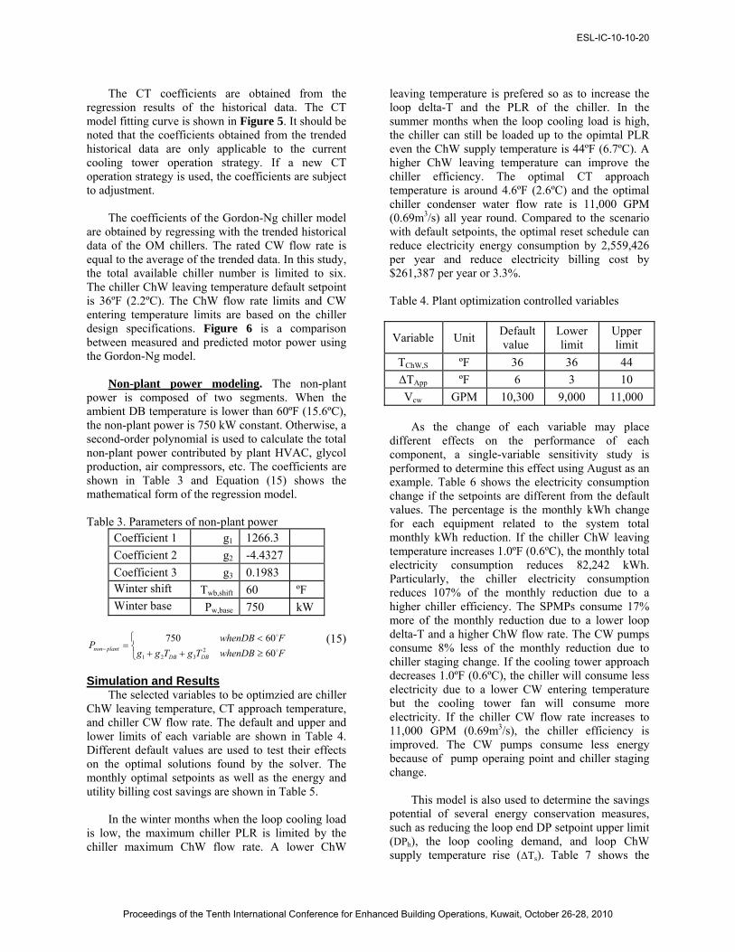
The CT coefficients are obtained from the regression results of the historical data. The CT model fitting curve is shown in Figure 5. It should be noted that the coefficients obtained from the trended historical data are only applicable to the current cooling tower operation strategy. If a new CT operation strategy is used, the coefficients are subject to adjustment.

The coefficients of the Gordon-Ng chiller model

are obtained by regressing with the trended historical data of the OM chillers. The rated CW flow rate is equal to the average of the trended data. In this study, the total available chiller number is limited to six. The chiller ChW leaving temperature default setpoint is 36ºF (2.2ºC). The ChW flow rate limits and CW entering temperature limits are based on the chiller design specifications. Figure 6 is a comparison between measured and predicted motor power using the Gordon-Ng model.

Non-plant power modeling. The non-plant

power is composed of two segments. When the ambient DB temperature is lower than 60ºF (15.6ºC), the non-plant power is 750 kW constant. Otherwise, a second-order polynomial is used to calculate the total non-plant power contributed by plant HVAC, glycol production, air compressors, etc. The coefficients are shown in Table 3 and Equation (15) shows the mathematical form of the regression model.

Table 3. Parameters of non-plant power

Coefficient 1 g1 1266.3 Coefficient 2 g2 -4.4327 Coefficient 3 g3 0.1983 Winter shift Twb,shift 60 ºF Winter base Pw,base 750 kW

⎩⎨⎧

≥++<

=− FwhenDBTgTggFwhenDB

PDBDB

plantnon o

o

6060750

2321

(15)

Simulation and Results The selected variables to be optimzied are chiller

ChW leaving temperature, CT approach temperature, and chiller CW flow rate. The default and upper and lower limits of each variable are shown in Table 4. Different default values are used to test their effects on the optimal solutions found by the solver. The monthly optimal setpoints as well as the energy and utility billing cost savings are shown in Table 5.

In the winter months when the loop cooling load

is low, the maximum chiller PLR is limited by the chiller maximum ChW flow rate. A lower ChW

leaving temperature is prefered so as to increase the loop delta-T and the PLR of the chiller. In the summer months when the loop cooling load is high, the chiller can still be loaded up to the opimtal PLR even the ChW supply temperature is 44ºF (6.7ºC). A higher ChW leaving temperature can improve the chiller efficiency. The optimal CT approach temperature is around 4.6ºF (2.6ºC) and the optimal chiller condenser water flow rate is 11,000 GPM (0.69m3/s) all year round. Compared to the scenario with default setpoints, the optimal reset schedule can reduce electricity energy consumption by 2,559,426 per year and reduce electricity billing cost by $261,387 per year or 3.3%.

Table 4. Plant optimization controlled variables

Variable Unit Default value

Lower limit

Upper limit

TChW,S ºF 36 36 44 ΔTApp ºF 6 3 10 Vcw GPM 10,300 9,000 11,000

As the change of each variable may place

different effects on the performance of each component, a single-variable sensitivity study is performed to determine this effect using August as an example. Table 6 shows the electricity consumption change if the setpoints are different from the default values. The percentage is the monthly kWh change for each equipment related to the system total monthly kWh reduction. If the chiller ChW leaving temperature increases 1.0ºF (0.6ºC), the monthly total electricity consumption reduces 82,242 kWh. Particularly, the chiller electricity consumption reduces 107% of the monthly reduction due to a higher chiller efficiency. The SPMPs consume 17% more of the monthly reduction due to a lower loop delta-T and a higher ChW flow rate. The CW pumps consume 8% less of the monthly reduction due to chiller staging change. If the cooling tower approach decreases 1.0ºF (0.6ºC), the chiller will consume less electricity due to a lower CW entering temperature but the cooling tower fan will consume more electricity. If the chiller CW flow rate increases to 11,000 GPM (0.69m3/s), the chiller efficiency is improved. The CW pumps consume less energy because of pump operaing point and chiller staging change.

This model is also used to determine the savings potential of several energy conservation measures, such as reducing the loop end DP setpoint upper limit (DPh), the loop cooling demand, and loop ChW supply temperature rise (ΔTs). Table 7 shows the

ESL-IC-10-10-20


Table 5. Monthly results of plant optimization

Month TChW,S ΔTApp Vcw Energy savings (kWh)

Billing cost savings ($)

Cost savings percentage

1 36.0 4.6 11,000 27,093 $ 6,912 1.9% 2 36.0 4.6 11,000 30,229 $ 7,159 1.9% 3 39.8 4.6 11,000 138,451 $ 16,132 2.8% 4 40.2 4.6 11,000 136,701 $ 15,563 2.8% 5 39.8 4.6 11,000 233,601 $ 23,172 3.1% 6 42.3 4.6 11,000 377,957 $ 34,289 3.9% 7 42.9 4.6 11,000 399,130 $ 36,903 3.9% 8 44.0 4.7 11,000 567,537 $ 51,490 4.9% 9 42.0 4.6 11,000 354,537 $ 32,368 3.8%

10 41.0 4.6 11,000 214,461 $ 21,568 3.2% 11 37.0 4.6 11,000 47,094 $ 8,483 1.7% 12 36.0 4.6 11,000 32,634 $ 7,347 1.9%

Total 2,559,426 $ 261,387 3.3%

Table 6. Results of single-variable sensitivity study

kWh savings

percentage Tchw=37.0ºF TApp=5.0ºF Vcw=11,000

GPM CHLR 107% 333% 76%

CT 0% -272% 1% CWP 8% 28% 21% PPMP 1% 10% 3% SPMP -17% 0% 0%

Savings (kWh) 82,242 23,414 93,393

Table 7. Billing cost savings estimation of energy conservation measures

Variable Unit Default Lower value Savings ($) Savings

(%)

DPh psid 28 26 $7,400 0.1% fLp,cooling - 1.00 0.95 $ 317,776 4.3% ΔTs ºF 1.0 0.5 $163,682 2.1%

annual billing cost savings potential. It is estimated that, when the loop DP upper limit decreases 2.0 psid (14 kPa), the savings are only 0.1%. If the loop cooling load reduce 5%, the savings are as large as 4.3%. When the loop supply temperature rise drop 0.5ºF (0.3ºC), the savings are 2.1%. These results can be used to estimate the payback of each measure.

SUMMARY AND CONCLUSION

A chilled water plant is a high energy density facility. However, the energy performance of most existing ChW plants is not very efficient. Improving the plant efficiency is an urgent task. Modeling and simulating is a popular method to optimize the plant operation and estimate the savings potential of various measures. The system-based model is simple but not accurate and the component-based model is accurate but complicated. This paper proposed a forward plant model based on a WTW efficiency concept. The WTW efficiency of each type of equipment is calculated with selected models or equations. This is a non-linear programming problem and can be solved with the GRG nonlinear solver. This forward plant model can be easily set up and used for plant energy simulation. It has an explicit physical meaning. Its application is not restricted by the equipment number and sequencing strategies. All calculations are explicit expressions and no iterations are required.

The application of this method is illustrated with

a practical project. The ChW system is modeled and three variables are selected for optimization. Compared to the baseline, a 3.3% of annual cost savings are achieved by implemeting the new reset schedules of the controlled variables. A single-variable sensitivity study shows that the reset of each variable can affect the energy consumption of several types of equipment. This model is also used to estimate the savings optential of several energy conservation measures.

NOMENCLATURE 4CP = four coincident peak

ESL-IC-10-10-20


C = cost, $

pc = water heat capacity, kJ/kg·K CHLR = chiller ChW = chilled water COP = coefficient of performance CT = cooling tower CV = coefficient of variation CW = condenser water CWP = condenser water pump d = cooling tower model coefficients DB = dry bulb DP = differential pressure e = loop hydraulic performance coefficient EP = energy plaza ERCOT = electric reliability council of Texas g = non-plant power model coefficients GPM = gallons per minute GRG = generalized reduced gradient h = loop delta-T model coefficient H = water head, feet HVAC = heating, ventilating, and air conditioning N = number NCP = non-coincident peak NLP = non linear programming NTU = number of transfer units OM = On-site Manufacture P = power, kW PID = proportional integral derivative PLR = part load ratio PPMP = primary pump Q = cooling load, ton R = electricity energy or demand rate, $/kWh

or $/kW SPMP = secondary pump T = temperature, ºF or ºC V = flow rate, GPM VSD = variable speed drive WB = wet Bulb WTW = wire-to-water x = independent variables

TΔ = temperature difference, ºF Greek symbols η = efficiency ξ = wire-to-water efficiency, kW/ton ρ = density, kg/m3

Subscripts App = approach

cdi = condenser water inlet cho = chilled water outlet

d = demand db = dry bulb e = energy Lp = loop max = maximum min = minimum mtr = motor R = return S = supply sys = system sp = setpoint wb = wet bulb

REFERENCES Ahn, B. C., and J. W. Mitchell. 2001. Optimal control

development for chilled water plants using a quadratic representation. Energy and Buildings 33(4): 371-78.

ASHRAE. 2003b. ASHRAE Handbook—HVAC Applications Chapter 41 Supervisory Control Strategies and Optimization. Atlanta, GA: American Society of Heating, Refrigerating and Air-Conditioning Engineers, Inc.

Bahnfleth, W. P., and E. B. Peyer. 2006. Energy use and economic comparison of chilled-water pumping system alternatives. ASHRAE Transactions 112(2): 198-208.

Bahnfleth, W. P., and E. B. Peyer. 2007. Energy use characteristics of variable primary flow chilled water pumping systems. Washington, DC: International Congress of Refrigeration.

Bradford, J. D. 1998. Optimal supervisory control of cooling plants without storage. Ph.D. Dissertation, Department of Civil, Environmental and Architectural Engineering, University of Colorado.

Braun, J. E. 1988. Methodologies for the design and control of central cooling plants. Ph.D. Dissertation, Department of Mechanical Engineering, University of Wisconsin-Madison.

Braun, J. E. 1989. Effectiveness models for cooling towers and cooling coils. ASHRAE Transactions 96(2): 164-174.

Braun, J. E., S. A. Klein, J. W. Mitchell, and W. A. Beckman. 1989c. Methodologies for optimal control to chilled water systems without storage. ASHRAE Transactions 95(1): 652-662.

Braun, J. E., J. W. Mitchell, S. A. Klein, and W. A. Beckman. 1987. Performance and control

ESL-IC-10-10-20


characteristics of a large central cooling system. ASHRAE Transactions 93(1): 1830-1852.

Chang, Y. 2006. An innovative approach for demand side management—optimal chiller loading by simulated annealing. Energy 31(12): 1883-1896.

Chang, Y., F. Lin, and C. Lin. 2005. Optimal chiller sequencing by branch and bound method for saving energy. Energy Conversion and Management 46(13-14): 2158-2172.

Cumali, Z. 1988. Global optimization of HVAC system operations in real time. ASHRAE Transactions 94(1): 1729-1744.

Durkin, T. H. 2005. Evolving design of chiller plants. ASHRAE Journal 47(11): 40-50.

Erpelding, B. 2006. Ultra efficient all-variable-speed chilled water plants. Heating Piping Air Conditioning 78(3): 35-43.

Furlong, J. W., and F. T. Morrison. 2005. Optimization of water-cooled chiller-cooling tower combinations. CTI Journal 26(1): 12-19.

Graves, R. D. 2003. Thermodynamic modelling and optimization of a screw compressor chiller and cooling tower system. M.S. Thesis, Department of Mechanical Engineering, Texas A&M University.

Hackner, R. J., J. W. Mitchell, and W. A. Bechman. 1985. HVAC system dynamics and energy use in buildings- Part II. ASHRAE Transactions 91(1): 781-795.

Hartman, T. B. 2001b. Ultra-efficient cooling with demand-based control. HPAC Engineering 73(12): 29-35.

Jiang, W., and T. A. Reddy. 2003. Re-evaluation of the Gordon-Ng performance models for water-cooled chillers. ASHRAE Transactions 109(2): 272-287.

Kirsner, W. 1995. Troubleshooting chilled water distribution problems at the NASA Johnson

Space Center. Heating Piping Air Conditioning 67(2): 51-59.

Kota, N. N., J. M. House, J. S. Arora, and T. F. Smith. 1996. Optimal control of HVAC systems using DDP and NLP techniques. Optimal Control Applications & Methods 17(1): 71-78.

Lau, A. S. 1985. Development of computerized control strategies for a large chilled water plant. ASHRAE Transactions 91(1): 766-780.

Lu, L., W. Cai, Y. C. Soh, and L. Xie. 2005b. Global optimization for overall HVAC systems––Part II problem solution and simulations. Energy Conversion and Management 46(7-8): 1015-1028.

Lu, L., W. Cai, Y. C. Soh, L. Xie, and S. Li. 2004. HVAC system optimization––condenser water loop. Energy Conversion and Management 45(4): 613-630.

Olson, R. T. 1993. A dynamic procedure for the optimal sequencing of plant equipment part1 algorithm fundametnals. Engineering Optimization 21(1): 63-78.

Sun, J., and A. Reddy. 2005. Optimal control of building HVAC&R systems using complete simulation based sequential quadratic programming (CSB-SQP). Building and Environment 40(5): 657-669.

Taylor, S. T. 2006. Chilled water plant retrofit—a case study. ASHRAE Transactions 112(2): 187-197.

Yu, F. W., and K. T. Chan. 2007. Optimum load sharing strategy for multiple-chiller systems serving air-conditioned buildings. Building and Environment 42(4): 1581-1593.

Yu, F. W., and K. T. Chan. 2008. Optimization of water-cooled chiller system with load-based speed control. Applied Energy 85(10): 931-950.

ESL-IC-10-10-20


optimization of a chilled water plant without storage ... · optimization of a chilled water plant...

Documents