BIS Papers No 2 165

Order flow and exchange rate dynamics

Martin D D Evans1 and Richard K Lyons

Abstract

Macroeconomic models of nominal exchange rates perform poorly. In sample, R2 statistics as high as10% are rare. Out of sample, these models are typically out-forecast by a naïve random walk. Thispaper presents a model of a new kind. Instead of relying exclusively on macroeconomic determinants,the model includes a determinant from the field of microstructure- order flow. Order flow is theproximate determinant of price in all microstructure models. This is a radically different approach toexchange rate determination. It is also strikingly successful in accounting for realised rates. Our modelof daily changes in log exchange rates produces R2 statistics above 50%. Out of sample, our modelproduces significantly better short-horizon forecasts than a random walk. For the DM/$ spot market asa whole, we find that $1 billion of net dollar purchases increases the DM price of a dollar by about0.5%.

Omitted variables is another possible explanation for the lack of explanatory powerin asset market models. However, empirical researchers have shown considerableimagination in their specification searches, so it is not easy to think of variables thathave escaped consideration in an exchange rate equation.

Richard Meese (1990)

1. Motivation: microstructure meets exchange rate economics

Since the landmark papers of Meese and Rogoff (1983a, 1983b), exchange rate economics has beenin crisis. It is in crisis in the sense that current macroeconomic approaches to exchange rates areempirical failures: the proportion of monthly exchange rate changes that current models can explain isessentially zero. In their survey, Frankel and Rose (1995) write “the Meese and Rogoff analysis atshort horizons has never been convincingly overturned or explained. It continues to exert a pessimisticeffect on the field of empirical exchange rate modelling in particular and international finance ingeneral.”2

Which direction to turn is not obvious. Flood and Rose (1995), for example, are “driven to theconclusion that the most critical determinants of exchange rate volatility are not macroeconomic.” Ifdeterminants are not macro fundamentals like interest rates, money supplies, and trade balances,then what are they? Two alternatives have attracted attention. The first is that exchange ratedeterminants include extraneous variables. These extraneous variables are typically modeled asrational speculative bubbles (Blanchard 1979, Dornbusch 1982, Meese 1986, and Evans 1986, amongothers). Though the jury is still out, Flood and Hodrick (1990) conclude that the bubble alternativeremains unconvincing. A second alternative to macro fundamentals is irrationality. For example,exchange rates may be determined in part from avoidable expectational errors (Dominguez 1986,Frankel and Froot 1987, and Hau 1998, among others). On a priori grounds, many economists findthis second alternative unappealing. Even if one is sympathetic to the presence of irrationality, there isa wide gulf between its presence and accounting for exchange rates empirically. Until it can producean empirical account, this too will remain an unconvincing alternative.

1 Respective affiliations are Georgetown University and NBER, and UC Berkeley and NBER. We thank the following for

valuable comments: two anonymous referees, Menzie Chinn, Peter DeMarzo, Frank Diebold, Petra Geraats, Eric Jondeau,Robert McCauley, Richard Meese, Michael Melvin, Peter Reiss, Andrew Rose, Mark Taranto, Ingrid Werner, Alwyn Young,and seminar participants at Chicago, Wharton, Columbia, MIT, Iowa, Houston, Stanford, UC Berkeley, the 1999 NBERSummer Institute (IFM), the December 1999 NBER program meeting in Microstructure, and the August 2000 BIS workshopon Market Liquidity. Lyons thanks the National Science Foundation for financial assistance.

2 The relevant literature is vast. Recent surveys include Frankel and Rose (1995), Isard (1995), and Taylor (1995).

166 BIS Papers No 2

Our paper moves in a new direction: the microeconomics of asset pricing. This direction makesavailable a rich set of models from the field of microstructure finance. These models are largely new toexchange rate economics, and in this sense they provide a fresh approach. For example,microstructure models direct attention to new variables, variables that have “escaped theconsideration” of macroeconomists (borrowing from the opening quote). The most important of thesevariables is order flow.3 Order flow is the proximate determinant of price in all microstructure models.(That order flow determines price is therefore robust to differences in market structure, which makesthis property more general than it might seem.) Our analysis draws heavily on this causal link fromorder flow to price. One level deeper, microstructure models also provide discipline for thinking abouthow order flow itself is determined. Information is key here - in particular, information that currencymarkets need to aggregate. This can include traditional macro fundamentals, but is not limited to them.In sum, our microeconomic approach provides a new type of alternative to the traditional macroapproach, one that does not rely on extraneous information or irrationality.4

Turning to the data, we find that order flow does indeed matter for exchange-rate determination. By“matter” we mean that order flow explains most of the variation in nominal exchange rates overperiods as long as four months. The graphs below provide a convenient summary of this explanatorypower. The solid lines are the spot rates of the DM and Yen against the Dollar over our four-monthsample (1 May to 31 August 1996). The dashed lines are marketwide order-flow for the respectivecurrencies. Order flow, denoted by x, is the sum over time of signed trades between foreign exchangedealers worldwide.5

Figure 1

Four months of exchange rates (solid) and order flow (dashed)1 May - 31 August 1996

DM/$ ¥/$

Order flow and nominal exchange rates are strongly positively correlated (price increases with buyingpressure). Macroeconomic exchange rate models, in contrast, produce virtually no correlation overperiods as short as four months.

3Order flow is a measure of buying/selling pressure. It is the net of buyer-initiated orders and seller-initiated orders. In adealer market such as spot foreign exchange, it is the dealers who absorb this order flow, and they are compensated fordoing so. (In an auction market, limit orders absorb the flow of market orders.)

4Another alternative to traditional macro modelling is the recent “new open-economy macro” approach (eg Obstfeld andRogoff 1995). We do not address this approach in this paragraph because, as yet, it has not produced an empiricalliterature.

5For example, if a dealer initiates a trade against another dealer's DM/$ quote, and that trade is a $ purchase (sale), thenorder flow is +1 (–1). These are cumulated across dealers over each 24-hour trading day (weekend trading - which isminimal - is included in Monday). In spot foreign exchange, roughly 75% of total volume is between dealers (25% isbetween dealers and non-dealer customers).

1.42

1.44

1.46

1.48

1.5

1.52

1.54

1.56

1 9 17 25 33 41 49 57 65 73

DM

/$

-1500

-1000

-500

0

500

1000

x

100

102

104

106

108

110

112

1 9 17 25 33 41 49 57 65 73

YE

N/$

-5000500100015002000250030003500

x

BIS Papers No 2 167

To address this more formally, we develop and estimate a model that includes both macroeconomicdeterminants (eg interest rates) and a microstructure determinant (order flow). Our estimates verify thesignificance of the above correlation. The model accounts for about 60% of daily changes in the DM/$exchange rate. For comparison, macro models rarely account for even 10% of monthly changes. Ourdaily frequency is noteworthy: though our model draws from microstructure, it is not estimated at thetransaction frequency. Daily analysis is in the missing middle between past microstructure work (tick-by-tick data) and past macro work (monthly data). Bridging the two helps clarify how lower-frequencyexchange rates emerge from the market’s operation in real time.

To complement these in-sample results, we also examine the model’s out-of-sample forecastingability. Work by Meese and Rogoff (1983a) examines short-horizon forecasts (1 to 12 months). Theyfind that a random walk model out-forecasts the leading macro models, even when macro-model“forecasts” are based on realised future fundamentals. Subsequent work lengthens the horizonbeyond 12 months and finds that macro models begin to dominate the random walk (Meese andRogoff 1983b, Chinn 1991, Chinn and Meese 1994, and Mark 1995). But results at shorter horizonsremain a puzzle. Here we examine horizons of less than one month. (Transaction data sets that arecurrently available are too short to generate statistical power at monthly horizons.) We find that athorizons from one-day to two-weeks, our model produces better forecasts than the random-walkmodel (over 30% lower root mean squared error).

The relation we find between exchange rates and order flow is not inconsistent with the macroapproach, but it does raise several concerns. Under the macro approach, order flow should not matterfor exchange rate determination: macroeconomic information is publicly available - it is impounded inexchange rates without the need for order flow. More precisely, the macro approach typically assumesthat: (1) all information relevant for exchange rate determination is common knowledge; and (2) themapping from that information to equilibrium prices is also common knowledge. If either of these twoassumptions is relaxed, however, then order flow will convey information about market-clearing prices.Relaxing the second assumption should not be controversial, given the failure of currentexchange-rate models. Direct evidence, too, corroborates that order flow conveys relevant information(Lyons 1995, Yao 1997, Covrig and Melvin 1998, Ito, Lyons and Melvin 1998, Cheung and Wong1998, Bjonnes and Rime 1998, Evans 1999, Naranjo and Nimalendran 1999, and Payne 1999.)6

Note that order flow being a proximate determinant of exchange rates does not preclude macrofundamentals from being the underlying determinant. Macro fundamentals in exchange rate equationsmay be so imprecisely measured that order-flow provides a better “proxy” of their variation. Thisinterpretation of order flow as a proxy for macro fundamentals is particularly plausible with respect toexpectations: standard empirical measures of expected future fundamentals are obviously imprecise.7

Orders, on the other hand, reflect a willingness to back one’s beliefs with real money (unlikesurvey-based measures of expectations). Measuring order flow under this interpretation is akin tocounting the backed-by-money expectational votes.

This paper has six remaining sections. Section two contrasts the micro and macro approaches toexchange rates. Section three develops a model that includes both micro and macro determinants.Section four describes our data. Section five presents our results. Section six provides perspective onour results. Section seven concludes.

6The standard example of order flow that conveys non-public information is orders from central bank intervention. (Within ourfour-month sample, however, the Fed never intervened.) Probably more important on an ongoing basis is order flow thatconveys information about “portfolio shifts” that are not common knowledge. A recent event provides a sharp example.Major banks attribute the yen/dollar rate’s drop from 145 to 115 in Fall 1998 to “the unwinding of positions by hedge fundsthat had borrowed in cheap yen to finance purchases of higher-yielding dollar assets” (The Economist, 10.10.98). Thisunwinding - and the selling of dollars that came with it - was forced by the scaling back of speculative leverage in themonths following the Long Term Capital Management crisis. These trades were not common knowledge as they wereoccurring. (See also section 6 below, and Cai et al. 1999.)

7One might argue that expectations measurement cannot be driving the negative results of Meese and Rogoff because theyuse the driving variables’ realised values. However, if the underlying macro model is incomplete, then realised values stillproduce an incorrect expectations measure.

168 BIS Papers No 2

2. Models: spanning the micro-macro divide

A core distinction between a microstructure approach to exchange rates and the traditional macroapproach is the role of trades in price determination. In macro models, trades have no distinct role indetermining price. In microstructure models, trades have a leading role - they are the proximate causeof price adjustment. It is instructive to frame this distinction by contrasting the structural models thatemerge from these two approaches.

Structural models: macro approach

Exchange-rate models within the macro approach are typically estimated at the monthly frequency.When estimated in changes they take the form:

(1) ∆pt = f(∆i, ∆m, …) + εt.

where ∆pt is the change in the log nominal exchange rate over the month (DM/$). The drivingvariables in the function f(∆i,∆m,…) include changes in home and foreign nominal interest rates i,money supply m, and other macro determinants, denoted here by the ellipsis.8 Changes in thesepublic-information variables drive price - there is no role for order flow. Any incidental price effectsfrom order flow that might arise are subsumed in the residual εt. These models are logically coherentand intuitively appealing. Unfortunately, they account for almost none of the monthly variation infloating exchange rates.

Structural models: microstructure approach

Equations of exchange-rate determination within the microstructure approach are derived from theoptimisation problem faced by price setters in the market - the dealers.9 These models are allvariations on the following specification:

(2) ∆pt = g(∆x, ∆I, …) + νt

Now ∆pt is the DM/$ rate change over two transactions, rather than over a month as in the macromodels. The driving variables in the function g(∆x,∆I,…) include order flow ∆x, the change in net dealerpositions (or inventory) ∆I, and other micro determinants, denoted by the ellipsis. Order flow can takeboth positive and negative values because the counterparty either purchases (+) at the dealer’s offeror sells at the dealer’s bid (–). Here we use the convention that a positive ∆x is net dollar purchases,making the theoretical relation positive: net dollar purchases drive up the DM price of dollars. It isinteresting to note that the residual in this case is the mirror image of the residual in equation 1: itsubsumes any price changes due to determinants in the macro model f(∆i,∆m,…), whereas theresidual in equation 1 subsumes price changes due to determinants in the micro model g(∆x,∆I,…).

Microstructure models predict a positive relation between ∆p and ∆x because order flowcommunicates non-public information, and once communicated, it is reflected in price. For example, ifthere is an agent who has superior information about the value of an asset, and that informationadvantage induces the agent to trade, then a dealer can learn from those trades (purchases indicategood news about the asset’s value, and vice versa). Empirically, estimates of a relation between ∆pand ∆x at the transaction frequency are uniformly positive and significant. This is true for manydifferent markets, including stocks, bonds, and foreign exchange.

The relation in microstructure models between ∆p and ∆I is not our focus in this paper, but let us clarifynonetheless. This relation is referred to as the inventory-control effect on price. The inventory-controleffect arises when a dealer adjusts his price to control fluctuation in his inventory. For example, if a

8The precise list of determinants depends on the model. Meese and Rogoff (1983a) focus on three models in particular: theflexible-price monetary model, the sticky-price monetary model, and the sticky-price asset model. Here our interest is simplya broad-brush contrast between the macro and microstructure approaches. For specific models see Frenkel (1976),Dornbusch (1976), and Mussa (1976), among many others.

9 Empirical work using structural micro models includes Glosten and Harris (1988), Madhavan and Smidt (1991), and Foster

and Viswanathan (1993), all of which address the NYSE. Structural models in a multiple-dealer setting include Snell andTonks (1995) for stocks, Lyons (1995) for currencies, and Vitale (1998) for bonds.

BIS Papers No 2 169

dealer has a larger long position than is desired, he may shade his bid and offer downward to induce acustomer purchase, thereby reducing his position. This affects realised transaction prices, whichaccounts for the relation. (These idiosyncratic inventory effects on individual dealer prices do not arisein the model developed in the next section.)

Spanning the micro-macro divide

To span the divide between the micro and macro approaches, we develop a model with componentsfrom both:10

(3) ∆pt = f(∆i,…) + g(∆x,…) + ηt.

The challenge is the frequency mismatch: transaction frequency for the micro models versus monthlyfrequency for the macro models. In the next section we develop a model in the spirit of equation (3).We estimate the model at the daily frequency by using micro determinants that are time-aggregated.We focus in particular on order flow ∆x. Our time-aggregated measure spans a much longer periodthan is addressed elsewhere within empirical microstructure.

3. Portfolio shifts model

Overview

One source of exchange rate variation in the model is portfolio shifts on the part of the public. Theseportfolio shifts have two important features. First, they are not common knowledge as they occur.Second, they are large enough that clearing the market requires adjustment of the spot exchange rate.

The first feature - that portfolio shifts are not common knowledge - provides a role for order flow. At thebeginning of each day, public portfolio shifts are manifested in orders in the foreign exchange market.These orders are not publicly observable. Dealers take the other side of these orders, and then tradeamong themselves during the day to share the resulting inventory risk. The market learns about theinitial portfolio shifts by observing this interdealer trading activity. By the end of the day, the dealers’inventory risk is shared with the public.

The second important feature is that the initial portfolio shifts, once absorbed by the public at the endof the day, are large enough to move price. This requires that the public’s demand for foreign-currencyassets is less than perfectly elastic. If the public’s demand is less than perfectly elastic, different-currency assets are imperfect substitutes, and price adjustment is required to clear the market.11 Inthis sense, our model is in the spirit of the portfolio balance approach to exchange rates. In anothersense, however, our model is very different from that earlier approach. Portfolio balance models aredriven by changes in asset supply. Asset supply is constant in our model. Rather, our model identifiestwo distinct components on the demand side. The first is driven by innovations in public information(standard macro fundamentals). The second is driven by non-public information. This non-publicinformation takes the form of portfolio shifts. The model does not take a stand on the underlyingdeterminants of these portfolio shifts (though we do address this issue in section 6).

10Goldberg and Tenorio (1997) develop a model for the Russian ruble market that includes both macro and microstructurecomponents. Osler’s (1998) trading model includes macroeconomic “current account traders” who affect the exchange ratein flow equilibrium.

11For evidence of imperfect substitutability across U.S. stocks, see Scholes (1972), Shleifer (1986) and Bagwell (1992),among others. Substitutability across currencies is likely to be lower than across same-currency stocks. Though directevidence of this lower substitutability is lacking, some point to home bias in international portfolios as indirect evidence.Note, too, that the size of the order flows the DM/$ spot market needs to absorb are on average more than 10,000 timesthose absorbed in a representative U.S. stock (eg the average daily volume on NYSE stocks in 1998 was $9.3 million,whereas the average daily volume in DM/$ spot was about $300 billion).

170 BIS Papers No 2

Specifics

Consider a pure exchange economy with T trading periods and two assets, one riskless, and one witha stochastic payoff representing foreign exchange. The T+1 payoff on foreign exchange, denoted F, is

composed of a series of increments, so that F=∑ +

=

1T

1t tr . The increments rt are i.i.d. Normal(0,Σr) and

are observed before trading in each period. These realised increments represent the flow of publiclyavailable macroeconomic information over time (eg changes in interest rates).

The foreign exchange market is organised as a decentralised dealership market with N dealers,indexed by i, and a continuum of non-dealer customers (the public), indexed by z∈ [0,1]. Within eachperiod (day) there are three rounds of trading. In the first round dealers trade with the public. In thesecond round dealers trade among themselves to share the resulting inventory risk. In the third rounddealers trade again with the public to share inventory risk more broadly. The timing within each periodis:

Daily timing

Round 1 Round 2 Round 3

rt Dealers Public Dealers Interdealer Order Dealers PublicQuote Trades Quote Trade Flow Quote Trades

The dealers and customers all have identical negative exponential utility defined over time-T wealth.

Trading round 1

At the beginning of each period t, all market participants observe rt, the period’s increment to thepayoff F. On the basis of this increment and other available information, each dealer simultaneouslyand independently quotes a scalar price to his customers at which he agrees to buy and sell anyamount.12 We denote this round-one price of dealer i as Pi1. (To ease the notational burden, wesuppress the period subscript t when clarity permits.) Each dealer then receives a net customer-orderrealisation ci1 that is executed at his quoted price Pi1, where ci1<0 denotes a net customer sale (dealeri purchase). Each of these N customer-order realisations is distributed Normal(0,Σc1), and they areindependent across dealers. (Think of these initial customer trades as assigned - or preferenced - to asingle dealer, resulting from bilateral customer relationships for example.) Customer orders are alsodistributed independently of the public-information increment rt.

13 These orders represent portfolioshifts on the part of the non-dealer public. Their realisations are not publicly observable.

Trading round 2

Round 2 is the interdealer trading round. Each dealer simultaneously and independently quotes ascalar price to other dealers at which he agrees to buy and sell any amount. These interdealer quotesare observable and available to all dealers in the market. Each dealer then simultaneously andindependently trades on other dealers’ quotes. Orders at a given price are split evenly across anydealers quoting that price. Let Ti2 denote the (net) interdealer trade initiated by dealer i in round two. Atthe close of round 2, all dealers observe the net interdealer order flow from that period:

12The sizes tradable at quoted prices in major FX markets are very large relative to other markets. At the time of our sample,the standard quote in DM/$ was good for up to $10 million, with a tiny bid-offer spread, typically less than four basis points.Introducing a bid-offer spread (or price schedule) in round one to endogenise the number of dealers is a straightforward -but distracting - extension of our model.

13A natural extension of this specification is that customer orders reflect changing expectations of future rt.

BIS Papers No 2 171

(4) ∑=

=∆N

iiTx

12

Note that interdealer order flow is observed without noise, which maximises the difference intransparency across trade types: customer-dealer trades are not publicly observed but interdealertrades are observed. In reality, FX trades between customers and dealers are not publicly observed.Though signals of interdealer order flow are publicly observed, it is not the case that these trades areobserved without noise. Adding noise to Eq. (4), however, has no qualitative impact on our estimatingequation, so we stick to this simpler specification.

Trading round 3

In round three, dealers share overnight risk with the non-dealer public. Unlike round one, the public’smotive for trading in round three is non-stochastic and purely speculative. Initially, each dealersimultaneously and independently quotes a scalar price Pi3 at which he agrees to buy and sell anyamount. These quotes are observable and available to the public at large.

The mass of customers on the interval [0,1] is large (in a convergence sense) relative to the N dealers.This implies that the dealers’ capacity for bearing overnight risk is small relative to the public’scapacity. Dealers therefore set prices so that the public willingly absorbs dealer inventory imbalances,and each dealer ends the day with no net position. These round-3 prices are conditioned on theround-2 interdealer order flow. The interdealer order flow informs dealers of the size of the totalinventory that the public needs to absorb to achieve stock equilibrium.

Knowing the size of the total inventory the public needs to absorb is not sufficient for determininground-3 prices. Dealers also need to know the risk-bearing capacity of the public. We assume it is lessthan infinite. Specifically, given negative exponential utility, the public’s total demand for the risky assetin round-3, denoted c3, is a linear function of the its expected return conditional on public information:

c3 = γ(E[P3,t+1|Ω3]-P3,t)

where the positive coefficient γ captures the aggregate risk-bearing capacity of the public, and Ω3 isthe public information available at the time of trading in round three.

Equilibrium

The dealer’s problem is defined over four choice variables, the three scalar quotes Pi1, Pi2, and Pi3,and the dealer’s interdealer trade Ti2 (the latter being a component of ∆x, the interdealer order flow).The appendix provides details of the model’s solution. Here we provide some intuition. Consider thethree scalar quotes. No arbitrage ensures that, within a given round, all dealers quote a commonprice. Given that all dealers quote a common price, this price is necessarily conditioned on commoninformation only. Though rt is common information at the beginning of round 1, order flow ∆xt is notobserved until the end of round 2. The price for round-3 trading, P3, therefore reflects the informationin both rt and ∆xt.

Whether ∆x does influence price depends on whether it communicates any price-relevant information.The answer is yes. Understanding why requires a few steps. First, the appendix shows that it isoptimal for each dealer to trade in round 2 according to the trading rule:

Ti2 = α ci1

with a constant coefficient α. Thus, each dealer’s trade in round 2 is proportional to the customer orderhe receives in round 1. This implies that when dealers observe the interdealer order flow ∆x=ΣiTi2 atthe end of round 2, they can infer the aggregate portfolio shift on the part of the public in round 1 (thesum of the N realisations of ci1). Dealers also know that the public needs to be induced to re-absorbthis portfolio shift in round 3. This inducement requires a price adjustment. Hence the relation betweenthe interdealer order flow and the subsequent price adjustment.

172 BIS Papers No 2

The pricing relation

The appendix establishes that the change in price from the end of period t-1 to the end of period t is:

(5) ∆Pt = rt + λ∆xt

where λ is a positive constant. That this price change includes the innovation in payoffs rt one-for-oneis unsurprising. The λ∆xt term is the portfolio shift term. This term reflects the price adjustmentrequired to induce re-absorption of the public’s portfolio shift from round 1. For intuition, note thatλ∆x=λΣiTi2=λαΣ ici1. The sum Σici1 is this total portfolio shift from round 1. The public’s total demand inround 3, c3, is not perfectly elastic, and λ insures that at the round-3 price c3+Σici1 =0.

Empirical implementation

Getting from equation (5) to an estimable model requires that we specialise the macro component ofthe model—the public-information increment rt. We choose to specialise this component to capturechanges in the nominal interest differential. That is, we define rt ≡ ∆(it–it*), where it is the nominal dollarinterest rate and it* is the nominal non-dollar interest rate (DM or Yen). This yields the followingregression model:

(6) ∆Pt = β1∆(it–it*) + β2∆xt + ηt

Our choice of specialisation has some advantages. First, this specification is consistent with monetarymacro models in the sense that these models call for estimating ∆P using the interest differential’schange, not its level. (As a diagnostic, though, we also estimate the model using the level of thedifferential, a la Uncovered Interest Parity; see footnote 17.) Second, in asset-approach macro modelslike the Dornbusch (1976) overshooting model, innovations in the interest differential are the mainengine of exchange rate variation.14 Third, from a purely practical perspective, data on the interestdifferential are readily available at the daily frequency, which is certainly not the case for the otherstandard macro fundamentals (eg real output, nominal money supplies, etc).

Naturally, this specification of our macro component of the model has some drawbacks. It is certainlytrue that, as a measure of variation in macro fundamentals, the interest differential is obviouslyincomplete. One can view it as an attempt to control for this key macro determinant in order toexamine the importance of micro determinants. One should not view it as establishing a fair horse racebetween the micro and macro approaches.

4. Data

Our data set contains time-stamped, tick-by-tick data on actual transactions for the two largest spotmarkets - DM/$ and ¥/$ - over a four-month period, 1 May to 31 August 1996. (For more detail than weprovide here, see Evans 1997.) These data were collected from the Reuters Dealing 2000-1 systemvia an electronic feed customised for the purpose. Dealing 2000-1 is the most widely used electronicdealing system. According to Reuters, over 90% of the world’s direct interdealer transactions takeplace through the system.15 All trades on this system take the form of bilateral electronicconversations. The conversation is initiated when a dealer uses the system to call another dealer torequest a quote. Users are expected to provide a fast two-way quote with a tight spread, which is inturn dealt or declined quickly (ie within seconds). To settle disputes, Reuters keeps a temporary recordof all bilateral conversations. This record is the source of our data. (Reuters was unable to provide theidentity of the trading partners for confidentiality reasons.)

14Cheung and Chinn (1998) corroborate this empirically. Their surveys of foreign exchange traders show that the importanceof individual macroeconomic variables shifts over time, but “interest rates always appear to be important.”

15Direct trading accounts for about 60% of interdealer trade and brokered trading accounts for the remaining 40%. As noted infootnote 3, interdealer transactions account for about 75% of total trading in major spot markets (at the time of our sample).Therefore, relative to the total market, our data set represents about 90% of 60% of 75%, or about 40%. For more detail onthe Reuters Dealing 2000-1 System see Lyons (1995) and Evans (1997).

BIS Papers No 2 173

For every trade executed on D2000-1, our data set includes a time-stamped record of the transactionprice and a bought/sold indicator. The bought/sold indicator allows us to sign trades for measuringorder flow. This is a major advantage: we do not have to use the noisy algorithms used elsewhere inthe literature for signing trades. A drawback is that it is not possible to identify the size of individualtransactions.16 For model estimation, order flow ∆x is therefore measured as the difference betweenthe number of buyer-initiated trades and the number of seller-initiated trades. This shortcoming of ourdata - as well as others - must be kept in perspective, however. If our data were noisy and our resultsnegative, then concern about data quality would be serious indeed - the negative results could easilybe due to poor data. We show below, however, that our results are quite positive. This cannot be theresult of noise in our data.

Three features of the data are especially noteworthy. First, they provide transaction information for thewhole interbank market over the full 24-hour trading day. This contrasts with earlier transaction datasets covering single dealers over some fraction of the trading day (Lyons 1995, Yao 1998, andBjonnes and Rime 1998). Our comprehensive data set makes it possible, for the first time, to analyseorder flow’s role in price determination at the level of “the market.” Though other data sets exist thatcover multiple dealers, they include only brokered interdealer transactions (see Goodhart, Ito andPayne 1996, and Payne 1999). More important, these other data sets come from a particularbrokered-trading system, one that accounts for a much smaller fraction of daily trading volume thanthe D2000-1 system covered by our data set. (There is also evidence that dealers attach moreinformational importance to direct interdealer order flow than to brokered interdealer order flow. SeeBjonnes and Rime 1998.)

Second, our market-wide transactions data are not observed by individual FX dealers as they trade.Though dealers have access to their own transaction records, they cannot observe others’transactions on the system. Our data therefore represent activity that, at the time, participants couldonly infer indirectly. This is one of those rare situations where the researcher has more informationthan market participants themselves (at least in this dimension).

Third, our data cover a relatively long time span (four months) in comparison with other micro datasets. This is important because the longer time span allows us to address exchange-ratedetermination from more of an asset-pricing perspective than was possible with previous micro dataspanning only days or weeks.

The three variables in our Portfolio Shifts model are measured as follows. The change in the spot rate(DM/$ or ¥/$), ∆pt, is the log change in the purchase transaction price between 4 pm (GMT) on day tand 4 pm on day t-1. When a purchase transaction does not occur precisely at 4 pm, we use thesubsequent purchase transaction (with roughly one million trades per day, the subsequent transactionis generally within a few seconds of 4 pm). When day t is a Monday, the day t-1 price is the previousFriday’s price. (Our dependent variable therefore spans the full four months of our sample, with noovernight or weekend breaks.) The daily order flow, ∆xt, is the difference between the number ofbuyer-initiated trades and the number of seller-initiated trades (in thousands), also measured from 4pm (GMT) on day t-1 to 4 pm on day t (negative sign denotes net dollar sales). The change in interestdifferential, ∆(it–it*), is calculated from the daily overnight interest rates for the dollar, thedeutschemark, and the yen (annual basis); the source is Datastream (typically measured atapproximately 4 pm GMT).

5. Empirical results

Our empirical results are grouped in four sets. The first set addresses the in-sample fit of the portfolioshifts model. The second set addresses robustness issues. The third set addresses the direction ofcausality. The fourth set of results addresses the model’s out-of-sample forecasting ability (in the spiritof Meese and Rogoff 1983a).

16This drawback may not be acute. There is evidence that the size of trades has no information content beyond that containedin the number of transactions. See Jones, Kaul, and Lipson (1994).

174 BIS Papers No 2

5.1 In-sample fit

Table 1 presents our estimates of the portfolio shifts model (equation 6) using daily data for the DM/$and ¥/$ exchange rates. Specifically, we estimate the following regression:

(7) ∆pt = β1∆(it–it*) + β2∆xt + ηt

where ∆pt is the change in the log spot rate (DM/$ or ¥/$) from the end of day t-1 to the end of day t,∆(it–it*) is the change in the overnight interest differential from day t-1 to day t (* denotes DM or ¥), and∆xt is the order flow from the end of day t-1 to the end of day t (negative denotes net dollar sales).17

The coefficient β2 on our portfolio shift variable ∆xt is correctly signed and significant, with t-statisticsabove 5 in both equations. To see that the sign is correct, recall from the model that net purchases ofdollars - a positive ∆xt - should lead to a higher DM price of dollars. The traditional macro-fundamental- the interest differential - is correctly signed, but is only significant in the yen equation. (The signshould be positive because, in the sticky-price monetary model for example, an increase in the dollarinterest rate it requires an immediate dollar appreciation - increase in DM/$ - to make room for theexpected dollar depreciation required by uncovered interest parity.) The overall fit of the model isstriking relative to traditional macro models, with R2 statistics of 64% and 45% for the DM and yenequations, respectively. In terms of diagnostics, the DM equation shows some evidence ofheteroskedasticity, so we correct the standard errors in that equation using a heteroskedasticity-consistent covariance matrix (White correction).18

Table 1

In-sample fit of portfolio shifts model∆pt = β1∆(it–it*) + β2∆xt + ηt

Diagnostics∆(it–it*) ∆xt

R2 Serial Hetero

DM 0.52 2.10 0.64 0.78 0.08(0.35) (0.20) 0.41 0.02

Yen 2.48 2.90 0.45 0.50 0.96(0.92) (0.46) 0.37 0.71

The dependent variable ∆pt is the change in the log spot exchange rate from 4 pm GMT on day t-1 to 4 pm GMT on day t (DM/$ or ¥/$). Theregressor ∆(it–it*) is the change in the one-day interest differential from day t-1 to day t (* denotes DM or ¥, annual basis). The regressor ∆xt isinterdealer order flow between 4 pm GMT on day t-1 and 4 pm GMT on day t (negative for net dollar sales, in thousands). Estimated using OLS.Standard errors are shown in parentheses (corrected for heteroskedasticity in the case of the DM). The sample spans four months (May 1 toAugust 31, 1996), which is 89 trading days. The Serial column presents the p-value of a chi-squared test for residual serial correlation, first-orderin the top row and fifth-order (one week) in the bottom row. The Hetero column presents the p-value of a chi-squared test for ARCH in theresiduals, first-order in the top row and fifth-order in the bottom row.

17Though the dependent variable in standard macro models is the change in the log spot rate, the dependent variable in thePortfolio Shifts model in equation (6) is the change in the spot rate without taking logs. These two measures for thedependent variable produce nearly identical results in all our tables (R2s, coefficient significance, lack of autocorrelation,etc). Here we present the log change results - equation 7 - to make them directly comparable to previous macrospecifications.

18To check robustness, we examine several obvious variations on the model. For example, in the spirit of Uncovered InterestParity, we include the level of the interest differential in lieu of its change. The level of the differential is insignificant in bothcases. We also include a constant in the regression, even though the model does not call for one. The constant isinsignificant for both currencies. Estimating the whole model in levels rather than changes produces a pattern similar to thatin Table 1: order flow is highly significant, the interest differential is insignificant, and R2 is 0.75 for the DM equation and 0.61for the Yen equation. With this levels regressions, however, beyond the usual concerns about non-stationarity, there is alsostrong evidence of serial correlation and heteroskedasticity (both tests are significant at the 1% level for both currencies).Finally, recall that our price series is measured from purchase transactions. Results using 4 pm sale prices are identical. Weaddress additional robustness issues in the next subsection.

BIS Papers No 2 175

The size of our order flow coefficient is consistent with past estimates based on single-dealer data.The coefficient of 2.1 in the DM equation implies that a day with 1000 more dollar purchases thansales induces an increase in the DM price by 2.1%. Given the average trade size in our sample of$3.9 million, $1 billion of net dollar purchases increases the DM price of a dollar by 0.54% (= 2.1/3.9).At a spot rate of 1.5 DM/$, this implies that $1 billion of net dollar purchases increases the DM price ofa dollar by 0.8 pfennig. At the single-dealer level, Lyons (1995) finds that information asymmetryinduces the dealer he tracks to increase price by 1/100th of a pfennig (0.0001 DM) for every incomingbuy order of $10 million. That translates to 1 pfennig per $1 billion. Though linearly extrapolating thisestimate is certainly not an accurate description of single-dealer behaviour, with multiple dealers itmay be a good description of the market’s aggregate elasticity.

The striking explanatory power of these regressions is almost wholly due to order flow ∆xt. Regressing∆pt on ∆(it–it*) alone, plus a constant, produces an R2 statistic less than 1% in both equations, andcoefficients on ∆(it–it*) that are insignificant at the 5% level.19 That the interest differential regainssignificance once order flow is included, at least in the Yen equation, is consistent with omittedvariable bias in the interest-rates-only specification. (The correlation between the two regressors ∆xt

and ∆(it–it*) is 0.02 for the DM and –0.27 for the Yen, though both are insignificant at the 5% level.)

Order flow’s ability to account for the full four months of exchange rate variation is surprising, not onlyfrom the perspective of macro exchange rate economics, but also from the perspective ofmicrostructure finance. Recall from section 2 that structural models within microstructure finance aretypically estimated at the transaction frequency - they make no attempt to account for prices over thefull 24-hour day. Our regression is at the daily frequency. One might have conjectured that the netimpact of order flow over the day would be zero (each day accounts for about one milliontransactions). This conjecture would be consistent with a belief that cumulative order flowmean-reverts rapidly (eg within a day). But rapid mean reversion is clearly not the behaviour displayedby cumulative order flow in Figure 1. This lack of mean reversion provides some room for the lowerfrequency relation we find here.

The lack of strong mean reversion in our measured order flow deserves further attention, particularlyconsidering that half-lives of individual dealer positions can be as short as 10 minutes (Lyons 1998).The key lies in recognising that our measure of order flow reflects interdealer trading, not customer-dealer trading. Consider a scenario that illustrates why our measure in Figure 1 can be so persistent.(Recall that Figure 1 displays cumulative order flow, defined as the sum of interdealer order flow, ∆xt,from 0 to t.) Starting the scenario from xt=0, an initial customer sale does not move xt from zerobecause xt measures interdealer order flow only. After the customer sale, then when dealer i unloadsthe position by selling to another dealer j, xt drops to –1. A subsequent sale by dealer j to anotherdealer, dealer k, reduces xt further to –2.20 If a customer happens to buy dealer k’s position from him,then xt remains at –2. In this simple scenario, order flow measured only from trades betweencustomers and dealers would have reverted to zero - the concluding customer trade offsets theinitiating customer trade. The interdealer order flow, however, does not revert to zero. Note, too, thatthis difference in the persistence of the two order-flow measures - customer-dealer versus interdealer -is also a property of the Portfolio Shifts model. In the Portfolio Shifts model, customer order flow inround three always offsets the customer order flow in round one. But the interdealer order flow, whichonly arises in round two, does not net to zero. This non-zero ∆xt serves as a carrier of value in ourestimating equation.

5.2 Robustness

In this section we address three robustness issues beyond those examined in the previous section.They correspond to the following three questions: (1) Might the order-flow/price relation be non-linear?

19There is a vast empirical literature that attempts to increase the explanatory power of interest rates in exchange rateequations by introducing interest rates as separate regressors, introducing non-linear specifications, etc. This literature hasnot been successful, so we do not pursue this line here. Note that the lack of explanatory power from traditionalfundamentals is not unique to exchange rate economics: Roll (1988) produces R2s of only 20% using traditional equityfundamentals to account for daily stock returns, a result he describes as a “significant challenge to our science”.

20This repeated passing of dealer positions in the foreign exchange market is referred to as the “hot potato” phenomenon.See Burnham (1991) and Lyons (1997).

176 BIS Papers No 2

(2) Does the relation depend on the gross level of activity? and (3) Does the relation depend on day ofthe week?

Might the order-flow/price relation be non-linear?

The linearity of our Portfolio Shifts specification depends crucially on several simplifying assumptions,some of which are rather strong on empirical grounds. It is therefore natural to investigate whethernon-linearities or asymmetries might be present.21 A simple first test is to add a squared order-flowterm to the baseline specification. The squared order-flow term is insignificant in both equations. Wealso test whether the coefficient on order flow is piece-wise linear, with a kink at ∆xt=0. If true, thismeans that buying pressure and selling pressure are not symmetric. A Wald test that the two slopecoefficients are equal cannot be rejected for the DM equation. There is some evidence of differentslopes in the Yen equation however: the test is rejected at the 4% marginal significance level. In thatcase, the point estimates show a greater sensitivity of price to order flow in the downward direction,though both estimates remain positive and significant.

Does the order-flow/price relation depend on the gross level of activity?

Another natural concern is whether the order-flow/price relation in Table 1 is state contingent in someway, perhaps depending on the market’s overall activity level. Our data set provides a convenientmeasure of overall activity, namely the total number of transactions. As a simple test, we partition oursample of trading days into quartiles, from days with the fewest transactions to days with the mosttransactions. We then estimate separate order-flow coefficients for each of these four samplepartitions. In both the DM and Yen equations, all four of the order-flow coefficients are positive. In theDM equation, the coefficients are slightly U-shaped (from fewest transactions to most, the pointestimates for β2 are 2.7, 2.0, 1.9, and 3.3). In the Yen equation, the coefficients are monotonicallyincreasing (from fewest transactions to most, the point estimates for β2 are 1.0, 1.1, 3.5, and 4.1).

In terms of theory, this result for the Yen is consistent with the “event-uncertainty” model of Easley andO’Hara (1992), but the DM result is not. The event-uncertainty model predicts that trades are moreinformative when trading intensity is higher. Key to understanding their result is that in their model,new information may not exist. If there is trading at time t, then a rational dealer raises her conditionalprobability that an information event has occurred, and lowers the probability of the “no-information”event. The upshot is that trades occurring when trading intensity is high induce a larger update inbeliefs, and therefore a larger adjustment in price.

Does the order-flow/price relation depend on day of the week?

Another state-contingency that warrants attention is day-of-the-week effects.22 To test whether day-of-the-week matters, we partition our sample into five sub-samples, one for each weekday (recall thatweekends are subsumed in our Friday-to-Monday observations). In both the DM and Yen equations,all five of the resulting order-flow coefficients are positive. In the DM equation, the Tuesday coefficientis the largest, and the Wednesday coefficient is the smallest. The Yen equation also shows thatTuesday’s coefficient is the largest, but in this case the Monday coefficient is smallest. More important,a Wald test that the coefficients are equal across the five days cannot be rejected at the 5% level ineither equation (though in the case of the Yen, it can be rejected at the 10% level).

5.3 Causality

Under our model’s null hypothesis, causality runs strictly from order flow to price. Accordingly, underthe null, our estimation is not subject to simultaneity bias. (We are not simply “regressing price onquantity,” as in the classic supply-demand identification problem. Quantity - ie volume - and order floware fundamentally different concepts.) Within microstructure theory more broadly, this direction of

21We pursue these (simple) non-linear specifications with the comfort that outliers are not driving our results - a fact that ismanifest from Figure 1.

22In terms of theory, the model of Foster and Viswanathan (1990) is a workhorse for specifying day-of-the-week effects. Intheir model, there is periodic variation in the information advantage of the informed trader. This advantage is assumed togrow over periods of market closure, in particular, over weekends, making order flow on Monday particularly potent.

BIS Papers No 2 177

causality is the norm: it holds in all the canonical models (Glosten and Milgrom 1985, Kyle 1985, Stoll1978, Amihud and Mendelson 1980), despite the fact that price and order flow are determinedsimultaneously. The important point in these models is that price innovations are a function of orderflow innovations, not the other way around.23 That said, alternative hypotheses do exist under whichcausality is reversed. The following taxonomy frames the causality issue, and identifies specificalternatives under which causality is reversed, so that the merits of these alternatives can be judged ina disciplined way.

Theoretical overview

The timing of the order-flow/price relation admits three possibilities, depending on whether order flowprecedes, is concurrent with, or lags price adjustment. We shall refer to these three timing hypothesesas the Anticipation hypothesis, the Pressure hypothesis, and the Feedback hypothesis, respectively.

Within each of the three hypotheses - Anticipation, Pressure, and Feedback - there are also variations.Under the Anticipation hypothesis, for example, order flow can precede price adjustment becauseprices adjust fully only after order flow is commonly observed - in low-transparency markets likeforeign exchange, order flow is not commonly observed when it occurs (Lyons 1996). Order flow mightalso precede price because price adjusts only after some piece of news anticipated by order flow iscommonly observed (eg the short-lived private information in Foster and Viswanathan 1990). Underthe Pressure hypothesis the two main variations correspond to microstructure theory’s canonicalmodel types - information models and inventory models. In information models, observing order flowprovides information about payoffs (Glosten and Milgrom 1985, Kyle 1985). In inventory models, orderflow alters equilibrium risk premia (Stoll 1978, Ho and Stoll 1981).24 Under the Feedback hypothesis,order flow lags price because of feedback trading. Negative-feedback trading is systematic selling inresponse to price increases, and buying in response to price decreases (eg Friedman’s celebrated“stabilising speculators”). Positive-feedback trading is the reverse. Variations on the Feedbackhypothesis are distinguished by whether this feedback trading is rational (an optimal response toreturn autocorrelation) or behavioural, meaning that it arises from systematic decision bias (DeLong etal. 1990, Jegadeesh and Titman 1993, Grinblatt et al. 1995).

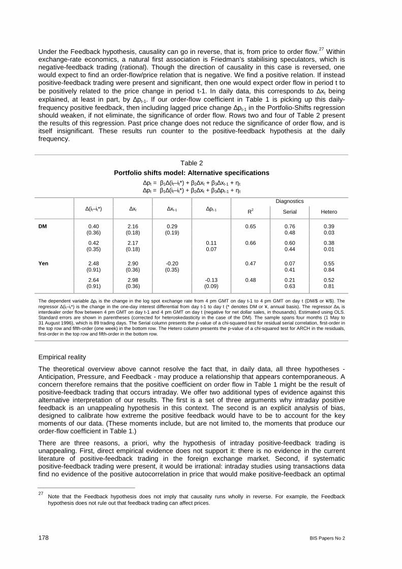
Under the Pressure hypothesis, causality runs from order flow to price, despite their concurrentrealisation.25 For the Anticipation hypothesis, the second variation noted above - where price adjustsonly after some piece of news anticipated by order flow is observed - is probably not relevant toforeign exchange (in contrast to equity markets, where insider order flow can anticipate a firm’searnings announcement, for example). The other variation of the Anticipation hypothesis - where orderflow affects price with a delay because it is not commonly observed - is relevant to foreign exchange.In this case, causality still runs from order flow to price, but the effects are delayed. As noted in theData section, order flow in this market is not common knowledge when realised. Consequently, lags inprice adjustment do not violate market efficiency (conditional on public information). One way to testthis variation of the Anticipation hypothesis is by introducing lagged order flow to our Portfolio Shiftsmodel. Rows one and three of Table 2 present the results of this regression: lagged order flow isinsignificant. At the daily frequency, lagged order flow is already embedded in price.26

23Put differently, order flow in these models is a proximate cause. The underlying driver of order flow is non-public information(information about uncertain demands, information about payoffs, etc). Order flow is the channel through which this type ofinformation is impounded in price.

24Within this inventory-model category, there is an additional distinction between price effects that arise at the marketmakerlevel (canonical inventory models) and price effects that arise at the marketwide level, due to imperfect substitutability(eg our Portfolio Shifts model). In the case of price effects at the marketmaker level, these effects are often modeled aschanging risk premia. But sometimes, largely for technical convenience, models are specified with risk-neutralmarketmakers who face some generic “inventory holding cost.”

25This does not imply that price cannot influence order flow. Price does influence order flow in microstructure models (both forthe usual downward sloping demand reason, and because agents learn from price). It is still the case that - in equilibrium -price innovations are functions of order flow innovations, not vice versa. Our Portfolio Shifts model is a case in point.

26As another check along these lines, we also decompose contemporaneous order flow into expected and unexpectedcomponents (by projecting it on past order flow). In our model, all order flow ∆x is unexpected, but this need not be the casein the data. We find, as the model predicts, that order flow’s explanatory power comes from its unexpected component.

178 BIS Papers No 2

Under the Feedback hypothesis, causality can go in reverse, that is, from price to order flow.27 Withinexchange-rate economics, a natural first association is Friedman’s stabilising speculators, which isnegative-feedback trading (rational). Though the direction of causality in this case is reversed, onewould expect to find an order-flow/price relation that is negative. We find a positive relation. If insteadpositive-feedback trading were present and significant, then one would expect order flow in period t tobe positively related to the price change in period t-1. In daily data, this corresponds to ∆xt beingexplained, at least in part, by ∆pt-1. If our order-flow coefficient in Table 1 is picking up this daily-frequency positive feedback, then including lagged price change ∆pt-1 in the Portfolio-Shifts regressionshould weaken, if not eliminate, the significance of order flow. Rows two and four of Table 2 presentthe results of this regression. Past price change does not reduce the significance of order flow, and isitself insignificant. These results run counter to the positive-feedback hypothesis at the dailyfrequency.

Table 2

Portfolio shifts model: Alternative specifications∆pt = β1∆(it–it*) + β2∆xt + β3∆xt-1 + ηt

∆pt = β1∆(it–it*) + β2∆xt + β3∆pt-1 + ηt

Diagnostics∆(it–it*) ∆xt ∆xt-1 ∆pt-1 R2 Serial Hetero

DM 0.40 2.16 0.29 0.65 0.76 0.39(0.36) (0.18) (0.19) 0.48 0.03

0.42 2.17 0.11 0.66 0.60 0.38(0.35) (0.18) 0.07 0.44 0.01

Yen 2.48 2.90 -0.20 0.47 0.07 0.55(0.91) (0.36) (0.35) 0.41 0.84

2.64 2.98 -0.13 0.48 0.21 0.52(0.91) (0.36) (0.09) 0.63 0.81

The dependent variable ∆pt is the change in the log spot exchange rate from 4 pm GMT on day t-1 to 4 pm GMT on day t (DM/$ or ¥/$). Theregressor ∆(it–it*) is the change in the one-day interest differential from day t-1 to day t (* denotes DM or ¥, annual basis). The regressor ∆xt isinterdealer order flow between 4 pm GMT on day t-1 and 4 pm GMT on day t (negative for net dollar sales, in thousands). Estimated using OLS.Standard errors are shown in parentheses (corrected for heteroskedasticity in the case of the DM). The sample spans four months (1 May to31 August 1996), which is 89 trading days. The Serial column presents the p-value of a chi-squared test for residual serial correlation, first-order inthe top row and fifth-order (one week) in the bottom row. The Hetero column presents the p-value of a chi-squared test for ARCH in the residuals,first-order in the top row and fifth-order in the bottom row.

Empirical reality

The theoretical overview above cannot resolve the fact that, in daily data, all three hypotheses -Anticipation, Pressure, and Feedback - may produce a relationship that appears contemporaneous. Aconcern therefore remains that the positive coefficient on order flow in Table 1 might be the result ofpositive-feedback trading that occurs intraday. We offer two additional types of evidence against thisalternative interpretation of our results. The first is a set of three arguments why intraday positivefeedback is an unappealing hypothesis in this context. The second is an explicit analysis of bias,designed to calibrate how extreme the positive feedback would have to be to account for the keymoments of our data. (These moments include, but are not limited to, the moments that produce ourorder-flow coefficient in Table 1.)

There are three reasons, a priori, why the hypothesis of intraday positive-feedback trading isunappealing. First, direct empirical evidence does not support it: there is no evidence in the currentliterature of positive-feedback trading in the foreign exchange market. Second, if systematicpositive-feedback trading were present, it would be irrational: intraday studies using transactions datafind no evidence of the positive autocorrelation in price that would make positive-feedback an optimal

27Note that the Feedback hypothesis does not imply that causality runs wholly in reverse. For example, the Feedbackhypothesis does not rule out that feedback trading can affect prices.

BIS Papers No 2 179

response (Goodhart, Ito, and Payne 1996). Third, the fallback possibility of irrational positive-feedbacktrading is difficult to defend. Recall that the order flow we measure is interdealer order flow. Thoughsystematic feedback trading of a behavioural nature (ie not fully rational) might be a good descriptionof some market participants, dealers are among the most sophisticated participants in this market.

Bias analysis

To close this section on causality, let us consider what it would take for positive-feedback trading toaccount for our results. Specifically, suppose intraday positive-feedback trading is present - Underwhat conditions could it account for the key moments of our data? These moments include, but are notlimited to, the moments that produce our positive order-flow coefficient in Table 1. We show below thatthese conditions are rather extreme. In fact, through a broad range of underlying parameter values,feedback trading would have to be negative to account for the key moments of our data.

We start by decomposing measured order flow ∆xt into two components:

(8) ∆xt = ∆xt1 + ∆xt2

where ∆xt1 denotes exogenous order flow from portfolio shifts (a la our model), with variance equal toΣx1, and ∆xt2 denotes order flow due to feedback trading, where

(9) ∆xt2 = γ∆pt

Suppose the true structural model can be written as:

(10) ∆pt = α∆xt1 + εt

where εt represents common-knowledge (CK) news, and εt is iid with variance Σε. By CK news wemean that both the information and its implication for equilibrium price is common knowledge. If bothconditions are not met, then order flow will convey information about market-clearing prices (recall thediscussion in the introduction). If feedback trading is present (γ≠0), then α will be a reduced formcoefficient that depends on γ. Note that under these circumstances, equation (10) is a valid reduced-from equation that could be estimated by OLS if one had data on ∆xt1.

With data on ∆xt and ∆pt only, suppose we estimate

(11) ∆pt = β∆xt + εt

If γ≠0, our estimates of β will suffer from simultaneity bias. To evaluate the size of this bias, considerthe implications of equations (8) through (10) for the moments:

β = Cov(∆pt,∆xt) / Var(∆xt)

δ = Var(∆pt) / Var(∆xt)

From equations (8) through (10) we know that:

∆xt = (1+γα)(∆xt1) + γεt

Solving for expressions for Cov(∆pt,∆xt), Var(∆pt), and Var(∆xt), we can write:

β = Cov(∆pt,∆xt) / Var(∆xt) = (α(1+γα)Σx1 + γΣε) / ((1+γα)2Σx1 + γ2Σε)

δ = Var(∆pt) / Var(∆xt) = (α2Σx1 + Σε) / ((1+γα)2Σx1 + γ2Σε)Now, define an additional parameter:

φ = Σε/Σx1

This parameter represents the ratio of CK news to order-flow news. With this parameter φ we canrewrite the key coefficients as:

β = (α(1+γα) + γφ) / ((1+γα)2 + γ2φ)

δ = (α2 + φ) / ((1+γα)2

+ γ2φ)

180 BIS Papers No 2

Using the sample moments for Cov(∆pt,∆xt), Var(∆pt), and Var(∆xt), we can solve for the impliedvalues of the α and γ for given values of φ. The following table presents these implied values of α andγ.

Note that even for values of φ above 2, the feedback trading needed to generate our results is actuallynegative. Note too that the parameter α - the order-flow-causes-price parameter - is not driven to zerountil φ reaches values well above 10. To invalidate our causality interpretation, then, CK news wouldhave to be one to two orders of magnitude more important that order-flow news. In our judgement thisis too extreme to be compelling.

To close this section on causality, it is not enough for the sceptical reader to assert simply that orderflow and price are both “endogenous,” or that we are merely observing a “simultaneous relationship”.These points are true. But they are also true within the body of microstructure theory reviewed above.And within that body of theory, price innovations are still driven by order flow innovations. This sectionis our effort to bring some disciplined thinking to an otherwise superficial debate.

Table 3

Bias analysis∆xt2 = γ∆pt

∆pt = α∆xt1 + εt

φ=Σε/Σx1 α γ

DM 0 2.4 –0.050.1 1.2 –0.511 1.9 –0.122 2.1 –0.0310 2.0 0.16

100 0.0 0.36

Yen 0 2.4 –0.180.1 1.3 –0.581 2.2 –0.232 2.4 –0.1510 2.8 –0.02

100 0.0 0.21

The table shows the values for the parameters α (order-flow-causes-price) and γ (price-causes-order-flow) implied by the sample moments andgiven values for the parameter φ. The parameter φ is the ratio of common-knowledge news to order-flow news.

5.4 Out-of-sample forecasts

To control for the myriad specification searches conducted by empiricists, a tradition within exchangerate economics has been to augment in-sample model estimates with estimates of models’out-of-sample forecasting ability. Accordingly, we present results along these lines as well. Theoriginal work by Meese and Rogoff (1983a) examines forecasts from 1 to 12 months. Our four-monthsample does not provide sufficient power to forecast at these horizons. Our horizons range insteadfrom one day to two weeks. The Meese-Rogoff puzzle is why short-horizon forecasts do so poorly, andour focus is definitely on the short end (though not so short as to render the horizon irrelevant from amacro perspective).

Table four shows that the portfolio shifts model produces better forecasts than the random-walk (RW)model. The forecasts from our model are derived from recursive estimates that begin with the first39 days of the sample. Like the Meese-Rogoff forecasts, our forecasts are based on realised values ofthe future forcing variables - in our case, realised values of order flow and changes in the interestdifferential. (Thus, they are not truly “out-of-sample forecasts”. We chose to stick with theMeese-Rogoff terminology.) The resulting root mean squared error (RMSE) is 30 to 40% lower thanthat for the random walk.

Note that our 89-day sample has very low power at the one- and two-week horizons. Even though ourmodel’s RMSE estimates are roughly 35% lower at these horizons, their out-performance is notstatistically significant. With a sample this size, the one-week forecast would need to cut the RW

BIS Papers No 2 181

model’s RMSE by about 50% to reach the 5% significance level. (To see this, note that for the DM atwo-standard-error difference at the one-week horizon is about 0.49, which is roughly half of the RWmodel’s RMSE of 0.98). The two-week forecast would have to cut the RW model’s forecast error bysome 54%. More powerful tests at these longer horizons will have to wait for longer spans oftransaction data.

Table 4

Out-of-sample forecasts errorsRoot mean squared errors (×100)

Horizon RW Portfolio shifts Difference

DM 1 day 0.44 0.29 0.15(0.033)

1 week 0.98 0.63 0.35(0.245)

2 weeks 1.56 0.96 0.60(0.419)

Yen 1 day 0.40 0.32 0.08(0.040)

1 week 0.98 0.64 0.33(0.239)

2 weeks 1.34 0.90 0.45(0.389)

The RW column reports the RMSE for the random walk model (approximately in %age terms). The Portfolio Shifts column reports the RMSE forthe model in equation (6). The Portfolio Shifts forecasts are based on realised values of the forcing variables. The forecasts are derived fromrecursive model estimates starting with the first 39 days of the sample. The Difference column reports the difference in the two RMSE estimates,and, in parentheses, the standard errors for the difference, calculated as in Meese and Rogoff (1988).

6. Discussion

The relation in our model between exchange rates and order flow is not easy to reconcile with thetraditional macro approach. Under the traditional approach, information is common knowledge and istherefore impounded in exchange rates without the need for order flow. This apparent contradictioncan be resolved if either: (1) some information relevant for exchange rate determination is not commonknowledge; or (2) some aspect of the mapping from information to equilibrium prices is not commonknowledge. If either is relaxed then order flow conveys information about market-clearing prices.

Our portfolio shifts model resolves the contradiction by introducing information that is not commonknowledge - information about shifts in public demand for foreign-currency assets. At a microeconomiclevel, dealers learn about these shifts in real time by observing order flow. As the dealers learn, theyquote prices that reflect this information. At a macroeconomic level, these shifts are difficult to observeempirically. Indeed, the concept of order flow is not recognised within the international macroliterature. (Transactions, if they occur at all, are strictly symmetric, and therefore cannot be signed toreflect net buying/selling pressure.)

If order flow drives exchange rates, then what drives order flow? From a valuation perspective, thereare two distinct views. The first view is that order flow reflects new information about valuationnumerators (ie future dividends in a dividend-discount model, which in foreign exchange take the formof future interest differentials). The second view is that order flow reflects new information aboutvaluation denominators (ie anything that affects discount rates). Our portfolio shifts model is anexample of the latter: order flow is unrelated to valuation numerators - the future rt. This type of orderflow can be rationalised with, for example, time-varying risk tolerance, time-varying hedging demands,or time-vary transactions demands. (In presenting the model, we did not take a stand on a specificrationalisation.) An example consistent with the valuation-numerators view is the“proxy-for-expectations” idea introduced in the introduction. That is, an important source of innovationsin exchange rates is innovations in expected future fundamentals, and in real time these may be wellproxied by order flow.

182 BIS Papers No 2

Note that separating valuation numerators from valuation denominators has implications for theconcept of “fundamentals.” Order flow that reflects information about valuation numerators - likeexpectations of future interest rates - is in keeping with traditional definitions of exchange-ratefundamentals. But order flow that reflects valuation denominators encompasses nontraditionalexchange-rate determinants, calling, perhaps for a broader definition. In any event, exploring theselinks to deeper determinants is a natural topic for future research. This will surely require a retreatback into intraday data.28

The practitioner view versus the academic view

Another perspective on order flow emerges from the difference between academic and practitionerviews on price determination. Practitioners often explain price increases with the familiar reasoningthat “there were more buyers than sellers.” To most economists, this reasoning is tantamount to “pricehad to rise to balance demand and supply.” But these phrases may not be equivalent. For economists,the phrase “price had to rise to balance demand and supply” calls to mind the Walrasian auctioneer.The Walrasian auctioneer collects “preliminary” orders and uses them to find the market-clearing price.Importantly, the auctioneer’s price adjustment is immediate - no trading occurs in the transition. (In arational-expectations model of trading, for example, this is manifested in all orders being conditionedon the market-clearing price.)

Many practitioners have a different model in mind. In the practitioner model there is a dealer instead ofan abstract auctioneer. The dealer acts as a buffer between buyers and sellers. The orders the dealercollects are actual orders, rather than preliminary orders, so trading does occur in the transition to thenew price. The dealer determines new prices from the new information about demand and supply thatbecomes available.

Can the practitioner model be rationalised? At first blush, it appears that trades are taking place out ofequilibrium, implying irrational behaviour. But this misses an important piece of the puzzle. Whetherthese trades are out-of-equilibrium depends on the information available to the dealer. If the dealerknows at the outset that there are more buyers than sellers (eventually pushing price up), then it maynot be optimal to sell at a low interim price. If the buyer/seller imbalance is not known, however, thenrational trades can occur through the transition. In this case, the dealer cannot set price conditional onall the information available to the Walrasian auctioneer. This is precisely the story developed incanonical microstructure models (Glosten and Milgrom 1985). Trading that would be irrational if thedealer could condition on the auctioneer’s information can be rationalised in models with more limited(and realistic) conditioning information.

Relation between our model and the flow approach to exchange rates

Consider the relation between our model, with its emphasis on order flow, and the traditional “flowapproach” to exchange rates. Is our approach just a return to the earlier flow approach? Despite theirapparent similarity, the two approaches are distinct and, in fact, fundamentally different.

A key feature of our model is that order flow plays two roles. First, holding beliefs constant, order flowaffects price through the traditional process of market clearing. Second, order flow also alters beliefsbecause it conveys information that is not yet common knowledge. That is:

Price = P(∆x, B(∆x,…), …)

Price P thus depends both directly and indirectly on order flow, ∆x, where the indirect effect is viabeliefs B. Early attempts to analyse equilibrium with differentially informed individuals ignored theinformation role - the effect of order flow on beliefs. Since the advent of rational expectations, modelsthat ignore this information effect from order flow are viewed as less compelling.

28The role of macro announcements in determining order flow warrants exploring. This, too, requires the use of intraday data.A second possible use of macro announcements is to introduce them directly into our Portfolio Shifts specification, even atthe daily frequency. This tack is not likely to be fruitful: there is a long literature showing that macro announcements areunable to account for exchange rate first moments (as opposed to second moments; see Andersen and Bollerslev 1998).

BIS Papers No 2 183

This is the essential difference between the flow approach to exchange rates and the microstructureapproach. Under the flow approach, order flow communicates no information back to individualsregarding others’ views/information. All information is common knowledge, so there is no informationthat needs aggregating. Under the microstructure approach, order flow does communicate informationthat is not common knowledge. This information needs to be aggregated by the market, andmicrostructure theory describes how that aggregation is achieved, depending on the underlyinginformation type.

7. Conclusion

This paper presents a model of exchange rate determination of a new kind. Instead of relyingexclusively on macroeconomic determinants, we draw on determinants from the field ofmicrostructure. In particular, we focus on order flow, the variable within microstructure that is - boththeoretically and empirically - the driver of price.29 This is a radical departure from traditionalapproaches to exchange rate determination. Traditional approaches, with their common-knowledgeenvironments, admit no role for information aggregation. Our findings suggest instead that the problemthis market solves is indeed one of information aggregation.

Our Portfolio Shifts model provides an explicit characterisation of this information aggregationproblem. The model is also strikingly successful in accounting for realised rates. It accounts for morethan 60% of daily changes in the DM/$ rate, and more than 40% of daily changes in the Yen/$ rate.Out of sample, our model produces better short-horizon forecasts than a random walk. Our estimatesof the sensitivity of the spot rate to order flow are sensible as well, and square with past estimates atthe individual-dealer level. We find that for the DM/$ market as a whole, $1 billion of net dollarpurchases increases the DM price of a dollar by about 0.5%. This relation should be of particularinterest to people working on central bank intervention (though care should be exercised in mappingcentral bank orders to subsequent interdealer trades).

Two issues raised by our measure of order flow deserve some remarks. First, though our measurecaptures a substantial share of total trading, it remains incomplete. As data sets covering customer-dealer trading and brokered interdealer trading become available, the order-flow picture can becompleted (see, eg Payne 1999). A second interesting issue raised by our order-flow measure iswhether its relation to price would change if order flow were observable to dealers in real time (ie if themarket were more transparent). From a policy perspective, the effects of increasing order-flowtransparency may be important: unlike most other financial markets, the FX market is unregulated inthis respect. The welfare consequences are not yet well understood.

So where do the results of this paper lead us? In our judgement they point toward a research agendathat borrows from both the macro and microstructure approaches. It is not necessary to decoupleexchange rates from macroeconomic fundamentals, as is common within microstructure finance. Inthis way, the approach is more firmly anchored in the broader context of asset pricing. (Though wefreely admit that longer time series will be necessary to implement the macro dimension fully.) Nor is itnecessary to treat exchange rates as driven wholly by public information, as is common within themacro approach. The information aggregation that arises when one reduces reliance on publicinformation is well suited to microstructure: there are ample tools within the microstructure approachfor addressing this aggregation. In the end, this two-pronged approach may help locate the missingmiddle in exchange rate economics - that disturbing space between our successful modelling of veryshort and very long horizons.

We close by addressing the obvious challenge for this agenda: What drives order flow? Here are twostrategies, among many, for shedding light on this question. The first strategy involves disaggregatingorder flow. For example, interdealer order flow can be split into large banks versus small banks, orinvestment banks versus commercial banks. Data sets on customer order flow can be split into non-financial corporations, leveraged financial institutions (eg hedge funds), and unleveraged financialinstitutions (eg mutual and pension funds). Do all these trade types have the same price impact? Ifnot, whose trades are most informative? This will clarify the underlying sources of non-CK information,

29This primacy of order flow within microstructure should mitigate standard concerns about data snooping. (In the words ofRichard Meese 1990, “At this point exchange rate modelers can be justly accused of in-sample data mining.”) The variablewe introduce - order flow - is the obvious a priori driving variable from microstructure theory.

184 BIS Papers No 2

which brings us closer to a specification of this market’s information structure. The second strategyinvolves focusing on periods where we expect CK information to be most important, for example,periods encompassing scheduled macro announcements. Does order flow account for a smaller shareof the price variation within these periods? Or is order flow an important channel for resolvinguncertainty about the mapping from public information to price? Whatever the result, the importantpoint is that the what-drives-order-flow question is not beyond our grasp.

BIS Papers No 2 185

Appendix: model solution

Each dealer determines quotes and speculative demand by maximising a negative exponential utilityfunction defined over terminal wealth. Because returns are independent across periods, with anunchanging stochastic structure, the dealers’ problem collapses to a series of independent tradingproblems, one for each period. Within a given period t, let Wiτ denote the end-of-round τ wealth ofdealer i, where we use the convention that Wi0 denotes wealth at the end of period t-1. (To ease thenotational burden, we suppress the period subscript t when clarity permits.) With this notation, andnormalising the gross return on the riskless asset to one, we can write the dealers’ problem as:

(A1)[ ]

3

2321 ,,,

)|exp(

iiii TPPP

iiWEMax Ω−− θ

s.t.

( )( ) ( )2322322221103 ]|[)( iiiiiiiiiiiii PPTPPTEDPPcWW −′−′−Ω′++′−+=

Piτ is dealer i’s round-τ quote and a ′ denotes an interdealer quote or trade received by dealer i. Thedealers’ problem is defined over four choice variables: the three scalar quotes Pi1, Pi2, and Pi3, and thedealer’s outgoing interdealer trade in round 2, Ti2. This outgoing interdealer trade in round 2 has threecomponents:

(A2) ]|[ 22212 Tiiiii TEDcT Ω′++=

where Di2 is dealer i’s speculative demand in round 2, and E[T′i2|ΩTi2] is the dealer’s attempt to hedge

against incoming orders from other dealers (this term is zero in equilibrium). The last three terms inWi3 capture capital gains/losses from round-1 customer orders ci1, round-2 speculative demand Di2,and the round-2 position disturbance from incoming interdealer orders T′

i2. The conditioninginformation Ωi at each decision node (3 quotes and 1 outgoing order) is summarised below.

ΩPi1 ≡ 1 kt

k r= , 11 k

tk x∆−

=

ΩPi2 ≡ ΩPi1, ci1

ΩTi2 ≡ ΩPi2

ΩPi3 ≡ ΩPi2, ∆xt

Conditional variances

This appendix repeatedly uses several conditional return variances. These variances do not dependon conditioning variables’ realisations (eg they do not depend on dealer i’s realisation of ci1. Theseconditional variances are therefore common to all dealers and known in period one. (It is a convenientproperty of the normal distribution that realisations of conditioning variables affect the conditionalmean but not the precision of the condition mean.) This predetermination of conditional variances iskey to the derivation of optimal quoting and trading rules.

Equilibrium

The equilibrium concept we use is Bayesian-Nash Equilibrium, or BNE. Under BNE, Bayes rule isused to update beliefs and strategies are sequentially rational given those beliefs.

Solving for the symmetric BNE, first we consider properties of optimal quoting strategies.

PROPOSITION 1: A quoting strategy is consistent with symmetric BNE only if the round-one andround-two quotes are common across dealers and equal to:

P1,t = P2,t = P3,t-1 + rt

186 BIS Papers No 2

where P3,t-1 is the round-three quote from the previous period, and rt is the public-informationinnovation at the beginning of period t.

PROPOSITION 2: A quoting strategy is consistent with symmetric BNE only if the commonround-three quote is:

P3,t = P2,t + λ∆xt

The constant λ is strictly positive.

Proof of propositions 1 and 2

No arbitrage requires that all dealers post a common quote in all periods. (Recall from section threethat all quotes are scalar prices at which the dealer agrees to buy/sell any amount, and trading withmultiple partners is feasible.) Common prices require that quotes be conditioned on commonlyobserved information only. In rounds one and two, this includes the previous period’s round-threeprice, plus the public-information innovation at the beginning of period t, rt. (Dealer i’s round-two quotetherefore cannot be conditioned on his realisation of ci1.)

The equations that pin down the levels of these three prices embed the dealer and customer tradingrules. When conditioned on public information, these trading rules must be consistent with equilibriumprice. This implies the following key relations:

(A3) E[ci1|ΩPi1] + E[Di2(P1,t)|ΩPi1] = 0

(A4) E[ci1|ΩPi1] + E[Di2(P2,t)|ΩPi1] = 0

(A5) E[Σici1|ΩPi3] + E[c3(P3,t)|ΩPi3] = 0

The first two equations simply state that, in expectation, dealers must be willing to absorb the demandfrom customers. The third equation states that, in expectation, the public must be willing at the round-3price to absorb the period’s aggregate portfolio shift. These equations pin down equilibrium pricebecause any price except that which satisfies each would generate net excess demand in round-2interdealer trading, which cannot be reconciled since dealers trade among themselves.

That P1,t=P2,t=P3,t-1+rt follows directly from the fact that expected value of ci1 conditional on publicinformation ΩPi1 is zero, and expected speculative dealer demand Di2 is also zero at this public-information-unbiased price. To be more precise, this statement postulates that the dealer’s demandDi2 has this property; we show below in the derivation of the optimal trading rule that this is the case.

That P3,t=P2,t+λ∆xt follows from the fact that ∆xt is a sufficient statistic for the period’s aggregateportfolio shift Σici1. Given the aggregate portfolio shift must be absorbed by the public in round 3, P3,t

must adjust to induce the necessary public demand. Specifically, the round-3 price must satisfy:

c3(P3,t) = –Σici1

Given the optimal rule for determining Ti2 (which we establish below), we can write Σici1 in terms ofinterdealer order flow ∆xt as:

Σici1 = (1/α)∆xt

and since the specification of c3 in the text is:

c3 = γ(E[P3,t+1|Ω3] –P3,t)this implies a market-clearing round-3 price of:

P3,t = E[P3,t+1|Ω3] + (αγ)-1∆xt

= ( )∑=∆+

t

1i ii xr λ

with λ=(αγ)-1, which is unambiguously positive. This sum is the expected payoff on the risky asset (theri terms), adjusted for a risk premium, which is determined by cumulative portfolio shifts (the ∆xi terms).This yields equation (5) in the text:

(5) ∆Pt = rt + λ∆xt

BIS Papers No 2 187

where ∆Pt denotes the change in price from the end of round three in period t-1 to the end of roundthree in period t.

Equilibrium trading strategies

An implication of common interdealer quotes P2,t is that in round two each dealer receives a share1/(N-1) of every other dealer’s interdealer trade. This order corresponds to the position disturbance T′

i2

in the dealer’s problem in equation (A1). Given the quoting strategy described in propositions one andtwo, the following trading strategy is optimal and corresponds to symmetric linear equilibrium:

PROPOSITION 3: The trading strategy profile:

Ti2 = α ci1

∀ i ∈ 1,...,N, with α>0, conforms to a Bayesian-Nash equilibrium.

Proof of proposition 3: optimal trading strategies

As noted above, because returns are independent across periods, with an unchanging stochasticstructure, the dealers’ problem collapses to a series of independent trading problems, one for eachperiod. Because there are only N dealers, however, each dealer acts strategically in the sense that hisspeculative demand depends on the impact his trade will have on subsequent prices.

It is well known that if a random variable W is distributed N(µ,σ2) and the utility function U(W)= –exp(–θW), then:

(A6) E[U(W)] = –exp[–θ(µ – θσ2/2)]Maximising E[U(W)] is therefore equivalent to maximising (µ – θσ2/2). This result allows us to write thedealers speculative-demand problem as:

(A7) Max i2D (E[P3|ΩTi2]–P2) – 2i2D (θ/2)σ2

Di2

where the information set ΩTi2 is defined above, and σ2 denotes the conditional variance of E[P3|ΩTi2]–P2. Now, from Proposition two, we can write:

(A8) E[P3|ΩTi2] – P2 = E[λ∆x|ΩTi2]

And from the definitions of ΩTi2 and ∆x we know that:

(A9) E[λ∆x|ΩTi2] = λTi2

The expected value of the other dealers’ trades in ∆x is 0 under our specification because (i) customertrades are mean-zero and independent across dealers and (ii) there is no information in the modelother than customer trades to motivate speculative demand. This fact also implies that dealer i’s tradein round 2, Ti2 from equation (A2), is equal to:

Ti2 = Di2 + ci1

Therefore, we can write the dealer’s problem as:

(A10) Max i2D λ(Di2 + ci1) – 2i2D (θ/2)σ2

Di2

The first-order condition of this problem is:

(A11) 2λDi2 + ci1 – θσ2Di2 = 0

which implies a speculative demand of:

(A12) 1222

1ii cD

−=

λθσ

188 BIS Papers No 2

This demand function and the fact that Ti2=Di2+ci1 imply:

(A13) 1122 12

1iii ccT α

λθσ≡

+

−=

The second-order condition for a maximum, (2λ–θσ2)<0, insures that α>0.

References

Amihud, Y and H Mendelson 1980, “Dealership market: Marketmaking with inventory”, Journal ofFinancial Economics, 8: 31-53.

Andersen, T and T Bollerslev 1998, “Deutsche mark-dollar volatility: Intraday activity patterns,macroeconomic announcements, and longer run dependencies”, Journal of Finance, 53: 219-266.

Bagwell, L 1992 “Dutch auction repurchases: An analysis of shareholder heterogeneity”, Journal ofFinance, 47: 71-105.

Bjonnes, G and D Rime 1998, “FX trading ... live: Impact of new trading environments, typescript”,Norwegian School of Management, December.

Blanchard, O 1979 “Speculative bubbles, crashes, and rational expectations”, Economics Letters, 14:387-389.

Burnham, J 1991 “Current structure and recent developments in foreign exchange markets, in S.Khoury” (ed.), Recent Developments in International Banking and Finance (North Holland,Amsterdam), 123-153.

Cai, J, Y Cheung, R Lee and M Melvin 1999, “Once-in-a-generation yen volatility in 1998:Fundamentals, intervention, or order flow?” typescript, Arizona State University, July.

Cheung, Y and M Chinn 1998 “Macroeconomic implications of the beliefs and behaviour of foreignexchange traders”, typescript, U.C. Santa Cruz, November.

Cheung, Y and C Wong 1998 “A survey of market practitioners’ views on exchange rate dynamics”,Journal of International Economics, forthcoming.

Chinn, M 1991 “Some linear and non-linear thoughts on exchange rates”, Journal of InternationalMoney and Finance, 10: 214-230.

Chinn, M and R Meese, 1994, “Banking on currency forecasts”, Journal of International Economics,38: 161-178.

Covrig, V and M Melvin 1998, “Asymmetric information and price discovery in the FX market: DoesTokyo know more about the yen?”, typescript, Arizona State University.

Degennaro, R and R Shrieves, 1997, “Public information releases, private information arrival, andvolatility in the foreign exchange market”, Journal of Empirical Finance, 4: 295-315.

DeLong, B, A Shleifer, L Summers and R Waldmann, 1990, “Positive feedback investment strategies,and destabilising rational speculation”, Journal of Finance, 45, 379-396.

Dominguez, K 1986, “Are foreign exchange forecasts rational?” New evidence from survey data,Economic Letters, 21: 277-281.

Dornbusch, R 1976, “Expectations and exchange rate dynamics”, Journal of Political Economy, 84:1161-1176.

Dornbusch, R 1982, “Equilibrium and disequilibrium exchange rates”, Zeitschrift fur Wirtschafts undSozialwissenschaften, 102: 573-799; reprinted in R. Dornbusch, Dollars, Debts and Deficits, MITPress: Cambridge, MA.

Easley, D and M O’Hara, 1992, “Time and the process of security price adjustment”, Journal ofFinance, 47: 577-605.

Evans, G 1986, “A test for speculative bubbles in the sterling-dollar exchange rate”, AmericanEconomic Review, 76: 621-636.

BIS Papers No 2 189

Evans, M 1997, “The microstructure of foreign exchange dynamics”, Georgetown University typescript,November, presented at the NBER Market Microstructure Conference, December 4, 1997.

Evans, M 1999, “What are the origins of foreign exchange movements?”, Georgetown Universitytypescript, March.

Fair, R 1970, “Estimation of simultaneous equations models with lagged endogenous variables andfirst order serially correlated errors”, Econometrica, 38: 507-516.

Flood, M 1994, “Market structure and inefficiency in the foreign exchange market”, Journal ofInternational Money and Finance, 13: 131-158.

Flood, R and R Hodrick, “On testing for speculative bubbles”, Journal of Economic Perspectives, 4:85-101.

Flood, R and A Rose, Fixing exchange rates: “A virtual quest for fundamentals”, Journal of MonetaryEconomics 36, 3-37.

Flood, R and M Taylor, 1996, “Exchange rate economics: What’s wrong with the conventional macroapproach?”, in Frankel, J G Galli and A Giovannini, (eds) The Microstructure of Foreign ExchangeMarkets (Chicago: The University of Chicago Press), 261-294.

Foster, D and S Viswanathan, 1990, “A theory of interday variations in volumes, variances, and tradingcosts in securities markets”, Review of Financial Studies, 3: 593-624.

Frankel, J and K Froot 1987, “Using survey data to test standard propositions regarding exchange rateexpectations”, American Economic Review, 77: 133-153.

Frankel, J, G Galli and A Giovannini 1996, “Introduction in The Microstructure of Foreign ExchangeMarkets” (Chicago: The University of Chicago Press), 1-15.

Frankel, J and A Rose 1995, “Empirical research on nominal exchange rates”, in G. Grossman and K.Rogoff (eds.), Handbook of International Economics, Elsevier Science: Amsterdam, 1689-1729.

Frenkel, J 1976, “A monetary approach to the exchange rate”: Doctrinal aspects and empiricalevidence, Scandinavian Journal of Economics, 78: 200-224.

Glosten, L and P Milgrom, 1985, “Bid, ask, and transaction prices in a specialist market withheterogeneously informed agents”, Journal of Financial Economics, 14: 71-100.

Goldberg, L and R Tenorio, 1997, “Strategic trading in a two-sided foreign exchange auction”, Journalof International Economics, 42: 299-326.

Goodhart, C 1988, “The foreign exchange market: A random walk with a dragging anchor”,Economica, 55: 437-460.

Goodhart, C, T Ito, and R Payne, 1996, “One day in June 1993”: A study of the working of the Reuters2000-2 electronic foreign exchange trading system. In The Microstructure of Foreign ExchangeMarkets, eds J Frankel, G Galli and A Giovannini, pp 107-179. University of Chicago Press, Chicago,IL.

Goodhart, C and M O’Hara 1997, “High frequency data in financial markets: Issues and applications”,Journal of Empirical Finance, 4: 73-114.

Grinblatt, M, S Titman and R Wermers, 1995, “Momentum investment strategies, portfolioperformance, and herding: A study of mutual fund behavior”, American Economic Review, 85, 1088-1105.

Hansch, O, N Naik and S Viswanathan 1998. “Do Inventories Matter in Dealership Markets? Evidencefrom the London Stock Exchange,” Journal of Finance, 53: 1623-1656.

Hau, H 1998, “Competitive entry and endogenous risk in the foreign exchange market”, Review ofFinancial Studies, 11: 757-788.

Ho, T and H Stoll, 1981, “Optimal dealer pricing under transactions and return uncertainty”, Journal ofFinancial Economics, 9, 47-73.

Hsieh, D and A Kleidon 1996, “Bid-ask spreads in foreign exchange markets: Implications for modelsof asymmetric information”, in Jeffrey Frankel et al eds: The Microstructure of Foreign ExchangeMarkets (University of Chicago Press, Chicago) 41-65.

190 BIS Papers No 2

Isard, P 1995, “Exchange Rate Economics”, Cambridge University Press: Cambridge, UK.

Ito, T, R Lyons and M Melvin, 1998, “Is there private information in the FX market?” The Tokyoexperiment, Journal of Finance 53, 1111-1130.

Jegadeesh, N and S Titman, 1993, “Returns to buying winners and selling losers: Implications forstock market efficiency”, Journal of Finance, 48, 65-92.

Jones, C, G Kaul and M Lipson, 1994, “Transactions, volume, and volatility”, Review of FinancialStudies, 7: 631-651.

Kouri, P 1976, “The exchange rate and the balance of payments in the short run and in the long run: Amonetary approach”, Scandinavian Journal of Economics, 78, 280-304.

Kouri, P and M Porter, 1974, “International capital flows and portfolio equilibrium”, Journal of PoliticalEconomy, 82, 443-467.

Kyle, A 1985, “Continuous auctions and insider trading”, Econometrica 53, 1315-1335.

Lyons, R 1995, “Tests of microstructural hypotheses in the foreign exchange market”, Journal ofFinancial Economics 39, 321-351.

Lyons, R 1996, “Optimal transparency in a dealer market with an application to foreign exchange”,Journal of Financial Intermediation, 5, 225-254.

Lyons, R 1997, “A simultaneous trade model of the foreign exchange hot potato”, Journal ofInternational Economics 42, 275-298.

Lyons, R 1998, “Profits and position control: A week of FX dealing”, Journal of International Moneyand Finance 17, 97-115.

Lyons, R 1999, “The Microstructure Approach to Exchange Rates”, MIT Press (chapters atwww.haas.berkeley.edu/~lyons/NewBook.html), forthcoming.

Mark, N 1995, “Exchange rates and fundamentals: Evidence on long-horizon predictability”, AmericanEconomic Review, 85: 201-218.

Meese, R 1986, “Testing for bubbles in exchange markets”, Journal of Political Economy, 94:345 -373.

Meese, R 1990, “Currency fluctuations in the post-Bretton Woods era”, Journal of EconomicPerspectives, 4: 117-134.

Meese, R and K Rogoff, 1983a, “Empirical exchange rate models of the seventies”, Journal ofInternational Economics, 14: 3-24.

Meese, R and K Rogoff, 1983b, “The out-of-sample failure of empirical exchange rate models, in J.Frenkel (ed.), Exchange Rate and International Macroeconomics”, University of Chicago Press:Chicago.

Meese, R and K Rogoff, 1988, “Was it real? The exchange rate-interest differential relation of themodern floating-rate period”, Journal of Finance, 43: 933-948.

Mussa, M 1976, “The exchange rate, the balance of payments, and monetary and fiscal policy under aregime of controlled floating”, Scandinavian Journal of Economics, 78: 229-248.

Naranjo, A and M Nimalendran, 1999, “Government intervention and adverse selection costs in foreignexchange markets”, Review of Financial Studies, forthcoming.

Obstfeld, M and K Rogoff, 1995, “Exchange rate dynamics redux”. Journal of Political Economy, 103:624-660.

Osler, C 1998, Short-term speculators and the puzzling behavior of exchange rates, Journal ofInternational Economics, 45: 37-57.

Payne, R 1999, Informed trade in spot foreign exchange markets: An empirical investigation,typescript, London School of Economics, January.

Peiers, B 1997, Informed traders, intervention, and price leadership: A deeper view of themicrostructure of the foreign exchange market. Journal of Finance 52, 1589-1614.

BIS Papers No 2 191

Reiss, P and I Werner, 1998, Does risk sharing motivate interdealer trading? Journal of Finance, 53:1657-1704.

Roll, R 1988, R2, Journal of Finance, 43: 541-566.

Romer, D 1993, Rational asset-price movements without news, American Economic Review, 83:1112-1130.

Scholes, M 1972, The market for securities: Substitution versus price pressure and the effect ofinformation on share price, Journal of Business, 45: 179-211.

Shleifer, A 1986, Do demand curves for stocks slope down? Journal of Finance, 41: 579-590.

Stoll, H 1978, The supply of dealer services in securities markets, Journal of Finance, 33, 1133-1151.

Taylor, M 1995, The economics of exchange rates, Journal of Economic Literature 33, 13-47.

Viswanathan, S and J Wang 1998, Why is interdealer trade so pervasive in financial markets?Working paper, Duke University.

Vitale, P 1998, Two months in the life of several gilt-edged market makers on the London StockExchange, Journal of International Financial Markets, Institutions, & Money, 8: 301-326.

Vogler, K 1997, Risk allocation and interdealer trading, European Economic Review 41, 417-441.

Wei, S and J Kim, 1997, The big players in the foreign exchange market: Do they trade on informationor noise?, NBER Working Paper 6256, November.

Yao, J 1998, Market making in the interbank foreign exchange market, New York University SalomonCenter Working Paper #S-98-3.

192 BIS Papers No 2

Comments on “Order flow and exchange rate dynamics”by Martin Evans and Richard Lyons

Eric Jondeau, Banque de France

At first glance, explaining the exchange-rate dynamics appears to be a challenge. Since the seminalwork by Meese and Rogoff (1983), we know that macro determinants are helpless to explain changesin exchange rate. Moreover, microstructure models are considered to be adequate to predictexchange rate, but only at a very high frequency.

This paper is very ambitious, since it aims at using a theoretical determinant of the exchange rate fromthe microstructure field to explain the exchange rate dynamics at a daily frequency. The authors arguethat this new determinant, the order flow, is helpful to forecast exchange rate, because it reveals toinvestors information on portfolio shifts, which is not common knowledge.

They develop a theoretical model based on the microstructure approach. In this model, the initialportfolio shifts by investors are not publicly observable. Market dealers take the other side of theseorders and then trade among themselves to share risk. Order flow is then defined as the sum of netintradealer trades.

Order flow is one of these theoretical concept, which measure is truly challenging. Here, themeasurement problem is overcome by the use of a perfectly adequate database. First, the databasecontains tick-by-tick data, which allows all transactions between dealers to be recorded. But, moreimportantly, for each transaction, a buyer/solder indicator is available, allowing trades to be signed andtherefore order flow to be measured.

The order flow is computed as the difference between the number of buyer-initiated trades and thenumber of solder-initiated trades. Therefore, the size of trades cannot be used to measure order flowmore accurately. In particular, during turbulent periods, there may be asymmetries between the size ofbuyer-initiated trades and the size of solder-initiated trades.

It is also worth noting that the period covered by the database is pretty long, since the data covers fourmonths for the DM-US and Yen-US exchange rates. Of course, a longer period of time would bedesirable to assess more precisely the ability of order flow to forecast exchange rate. But empiricalresults obtained for the two more traded currencies are rather convincing. A longer sample wouldallow several specification of the portfolio shift model to be tested. In particular, the effect of order flowmay well be a non-linear one.

At this stage, two issues arise: First, can the new explanatory variable be considered as exogenouswith respect to the exchange rate? Second, can the empirical evidence obtain by Evans and Lyonsbeen seen as solving the puzzle highlighted by Meese and Rogoff?

1. Exogeneity of order flow

I begin with the exogeneity of order flow. Empirical estimates of the portfolio-shift model are quiteimpressive: the authors obtain a strong and significant effect of the order flow in explaining change inexchange rate. The interest-rate spread has a correctly signed effect, but it is weakly significant. R2sare very large, as compared to usual standards. The portfolio-shift model appears to have a muchlarger explanatory power than standard macro models.

But this raises the issue of order flow exogeneity with respect to the exchange rate. In other words,can order flow be used in forecast exercises? The authors give several convincing arguments whycausality goes from order flow to price, and not from price to order flow. However, order flow may welldepend, to some extent, on prices. In this case, using order flow to forecast exchange rates wouldappear to be less promising. In particular, out-of-sample forecasts computed by the authors reveal thatthe portfolio shift model outperforms significantly, but rather weakly, the usual random walk. But thisexercise is performed using realized order flow and interest rates. A real-time forecast would require apreliminary forecast of order flow and interest rates. This would further reduce the forecast ability oforder flow. Yet this reduction would be even larger if order flow has to be forecast using past exchangerates.

BIS Papers No 2 193

2. The Meese and Rogoff puzzle

Concerning the Meese and Rogoff puzzle, I would like to make two remarks.

First, Meese and Rogoff stated that macro models fail to predict exchange rate. The failure of macromodels seems to come from their inability to represent exchange rate expectations accurately. Thispaper proposes a new proxy for exchange-rate expectations, the order flow, which seems to be muchmore accurate than previous proxy variables. From this point of view, this paper succeeds in solvingthe Meese and Rogoff puzzle, since it exhibits a theoretically and empirically pertinent determinant ofexchange rate.

On the other hand, this study has to be extended to longer periods and, more importantly, to othercurrencies. Indeed, it is usual in the exchange-rate analysis to obtain that a theoretical model is validfor one exchange rate but not for other ones. This is the sense of the result of Meese and Rogoff(1983).

Conclusion

To sum up, the approach developed in this paper is very appealing, since it shows that a natural microdeterminant of exchange rate is able to explain a large part of the exchange-rate dynamics.

Two avenues can be explored to answer the question “What drives order flow?” On one hand, assuggested by the authors, further disaggregating order flow would provide information on the kind oftrades which is more informative on future exchange rate. On the other hand, one may try to identifymacro determinants of order flow. The next step may be to derive the central tendency of exchangerate, which results from all transactions between individual customers and dealers interacting in themarket place. This central tendency may be a major determinant of order flow. Since the centraltendency has to be modeled in the macro area, this may help to fill the gap between micro and macroapproaches.

To conclude, I would like to ask a few questions. First, since the portfolio shift model appears to havea strong forecast ability, how could it be used in practice to forecast exchange rate? More precisely,are the data used to compute order flow available in real time, in order to take advantage of theforecast ability at the one-day horizon, for instance?

194 BIS Papers No 2

Comments on “Order flow and exchange rate dynamics”by Martin Evans and Richard Lyons

Robert N McCauley

This is a rare empirical study of exchange rate economics that leaves the reader with the feeling thathe has actually learned something about the subject. It also passes the Leontief test of working toanalyse new data rather than just re-squeezing a well-squeezed orange. Let me comment on thetheory, data and findings as presented and then make some suggestions as to how the analysis mightevolve to address the central concerns of this workshop.

Theory

Evans and Lyons are ambivalent about the theoretical position of order flow. In places it is theexpression of other determinants of exchange rates. In other places, it is a competing explanation.Conceiving of order flow as an explanation of exchange rate movements strikes me as similar toconceiving of the number of automobiles on the road in a city as an explanation of variations in thespeed of traffic. True, there are ways of thinking about exchange rate movements or traffic jams thatignore order flow or vehicular density. But a traffic engineer wants to know why drivers are out thereon the road. It is useful to know that order flow is a proximate cause of exchange rate changes, butone hopes that we can use data on order flow to point to the more remote causes, which may or maynot be fundamentals. Conceptually, order flow can be seen as tapping into portfolio shifts - and I findodd the assertion that “Portfolio balance models are driven by asset supply” (p8). Empirical tests of theportfolio theory have sought to find the effect of varying asset supplies, it is true, but the theorycontains predictions about the effect of demand shifts, which this paper can be read as verifying.

Data

After applauding the effort entailed in obtaining the Reuters 2000 data, let us put them into context.We are told in the text that the share of Reuters 2000 in direct interdealer trading is 90%--but whatshare of the spot market is captured? The data are drawn from a period, May-August 1996, when thespot foreign exchange market was undergoing rapid structural change. In particular, electronic brokingwas growing, apparently not only at the expense of voice broking but also at the expense of directdealing (BIS (1997), p91).

Lets look at the figures. In 1995 and 1998, 65% and 68% of dollar-DM and dollar-yen spot trading wasinterdealer: therefore the Reuters 2000 data on trading among dealers do not cover one-third of thespot market (BIS (1996, 1999), Table 1-B, Table E-2). Then, within the interdealer market, brokersaccount for a third of trades in 1995, rising to about a half in 1998 (Table). So the Reuters data coverwell less than half of the spot market overall and one-half to two-thirds of the interdealer market(accepting Reuters estimate of its share of the direct interdealer market).

The authors recognise the drawback of having data only on buy/sell hits (p14). The authors’ owntheorising says that dollars, not hits, matter, and I can only agree. Especially in light of the Reuters2000 system capturing only a part, albeit a very significant part, of all transactions, we have an errorsin variable problem here at the very least.

One small but significant suggestion regarding interest rates. Overnight rates do not well capturechanges in the expected path of policy rates. Something like the three-month rate, three monthsforward, better captures the swings in policy expectations that move interest rates.

Results

Whatever the slippage between what the authors want to measure and what they do measure, theirresults suggest the weight of order flow moves the exchange rate. Certainly market participants spenda lot of time and analysts devote a lot of words to assessing how other market participants arepositioning and repositioning.

BIS Papers No 2 195

The Study Group on Market Dynamics of the Working Group on Highly Leveraged Institutions (HLIs)learned that HLIs can release their private information on their own positions and intentions to theirown benefit. Furthermore, to my mind, it was evident that the sheer weight of HLI positions, particularlyin middle-sized markets, could absorb large fractions of the institutionally determined capacity ofday-to-day market participants, including exporters and portfolio managers, to take the other side.Under these circumstances, price formation could be very sensitive to news, rumours, or further, noisypositioning. The authors refer to the dollar-yen’s sharp move in Fall 1998, but the charts covering thatperiod for the Australian, New Zealand, Singaporean dollars and the South African rand also deservea look (Market Dynamics (2000)). Order flow and cumulated order flow matter.

What is missing from these results, however, is an active exploitation of the insight that liquidity in amarket is variable over time. Let me close on the interaction of order flow and liquidity.

The interaction of order flow and liquidity

The paper makes its most salient contribution to today’s discussion when it separates the data intoquartiles based on daily transactions volumes. The authors find a U-shaped pattern of coefficients onorder flow for the DM, indicating the largest impacts of order flow on days with the lightest andheaviest trading, and an upward pattern for the yen, indicating the strongest impact amid heaviesttrading. This is a rough cut, however, particularly if Reuters 2000 gains (or loses) market share duringperiods of high volatility.

It is known, however, that trading activity varies more by the hour of the day than by day. Consider theclaim of the Reserve Bank of Australia that highly leveraged institutions in mid-1998 deliberatelytraded during Sydney lunch time, or in the slow period between Sydney’s wind-down and London’swind-up, in order to have maximum effect on the Australian dollar’s exchange rate (Market Dynamics(2000), pp127-8). To address these claims, one would want to approach this question of the variableimpact of order flow by time of day.

A finer approach might also seek to separate out the response of order flow to major releases of newsbuilding ono the findings of Fleming and Remolona. Liquidity and order flow dynamics might differquite a bit between normal periods and immediate post-news periods.

In short, the authors should arm themselves with curiosity regarding the waxing and waning of liquidityand see what their data set can tell them. While this paper has made an important contribution to ourunderstanding of exchange rate determination, much work on foreign exchange market liquidityremains to be done.

References

Bank for International Settlements (1996). “Central Bank Survey of Foreign Exchange and DerivativesMarket Activity”, May.

Bank for International Settlements (1999). “Central Bank Survey of Foreign Exchange and DerivativesMarket Activity”, May.

Bank for International Settlements (1997): “67th Annual Report”, June.

Bank of England (1998). “The Foreign Exchange and Over-The-Counter Derivatives Markets in theUnited Kingdom”, Bank of England Quarterly Bulletin, November.

Bank of Japan (1998). “Foreign Exchange and Derivatives Markets Turnover Survey”, Bank of JapanQuarterly Bulletin, November, pp. 219-227.

Evans, Martin D D, and Richard K Lyons (1999). “Order Flow and Exchange Rate Dynamics”,December (processed).

Federal Reserve Bank of New York (1998). “Foreign Exchange and Interest Rate Derivatives MarketsSurvey Turnover in the United States”, 29 September.

Market Dynamics Study Group, Working Group on Highly Leveraged Institutions, Financial StabilityForum (2000). Report, April (www.fsforum.org/Reports/RepHLI05.pdf).

196 BIS Papers No 2

TableSpot interdealer foreign exchange trading by mode, 1995 and 1998

1995 1998

UK US JP UK US JP

Direct 63 64 53 54

Brokered 37 36 47 46

Of which: electronic 10 12 25 33 36

Sources: Bank of England (1998), p 352; Federal Reserve Bank of New York (1998), pp 6, 8; Bank of Japan (1998), p 224; BIS (1999), p 15.

Note: UK and US data are for spot trading as a whole; US voice broker share for spot trading assumed to be same as for all trading.