Out-of-Sample Exchange Rate Predictability

with Taylor Rule Fundamentals

Tanya Molodtsova* Emory University

David H. Papell**

University of Houston

November 25, 2008

Abstract

An extensive literature that studied the performance of empirical exchange rate models following Meese and Rogoff’s (1983a) seminal paper has not convincingly found evidence of out-of-sample exchange rate predictability. This paper extends the conventional set of models of exchange rate determination by investigating predictability of models that incorporate Taylor rule fundamentals. We find evidence of short-term predictability for 11 out of 12 currencies vis-à-vis the U.S. dollar over the post-Bretton Woods float, with the strongest evidence coming from specifications that incorporate heterogeneous coefficients and interest rate smoothing. The evidence of predictability is much stronger with Taylor rule models than with conventional interest rate, purchasing power parity, or monetary models.

We are grateful to Menzie Chinn, Todd Clark, Charles Engel, Martin Evans, Lutz Kilian, Nelson Mark, Mike McCracken, John Rogers, Moto Shintani, Vadym Volosovych, Jian Wang, Ken West, two anonymous referees, and participants at the 2006 Econometric Society Summer Meetings, International Economics and Finance Society sessions at the 2006 SEA and 2007 ASSA meetings, 2007 NBER Summer Institute, 2007 Bank of Canada-ECB Workshop on Exchange Rate Modeling, and Texas Camp Econometrics XI for helpful comments and discussions.

*Department of Economics, Emory University, Atlanta, GA 30322-2240. Tel: +1 (404) 727-8808. Email: tmolodt@emory.edu **Department of Economics, University of Houston, Houston, TX 77204-5882. Tel: +1 (713) 743-3807. Email: dpapell@uh.edu

1

1. Introduction

The failure of open-economy macro theory to explain exchange rate behavior using economic

fundamentals has prevailed in the international economics literature since the seminal papers by Meese and

Rogoff (1983a, 1983b), who examine the out-of-sample performance of three empirical exchange rate models

during the post-Bretton Woods period and conclude that economic models of exchange rate determination of

the 1970’s vintage do not perform better than a random walk model. While, starting with Mark (1995), a

number of studies have found evidence of greater predictability of economic exchange rate models at longer

horizons, these findings have been questioned by Kilian (1999). The recent comprehensive study by Cheung,

Chinn and Pascual (2005) examines the out-of-sample performance of the interest rate parity, monetary,

productivity-based and behavioral exchange rate models and concludes that none of the models consistently

outperforms the random walk at any horizon.

There is a disconnect between most research on out-of-sample exchange rate predictability, which is

based on empirical exchange rate models of the 1970s, and the literature on monetary policy evaluation,

which is based on some variant of the Taylor (1993) rule. A recent literature uses Taylor rules to model

exchange rate determination. The Taylor rule specifies that the central bank adjusts the short-run nominal

interest rate in response to changes in inflation and the output gap. By specifying Taylor rules for two

countries and subtracting one from the other, an equation is derived with the interest rate differential on the

left-hand-side and the inflation and output gap differentials on the right-hand-side. If one or both central

banks also target the purchasing power parity (PPP) level of the exchange rate, the real exchange rate will also

appear on the right-hand-side. Positing that the interest rate differential equals the expected rate of

depreciation by uncovered interest rate parity (UIRP) and solving expectations forward, an exchange rate

equation is derived.

Engel and West (2005) use the Taylor rule model as an example of present value models where asset

prices (including exchange rates) will approach a random walk as the discount factor approaches one. Engel

and West (2006) construct a “model-based” real exchange rate as the present value of the difference between

home and foreign output gaps and inflation rates, and find a positive correlation between the “model-based”

rate and the actual dollar-mark real exchange rate. Mark (2007) considers Taylor rule interest rate reaction

functions for Germany and the U.S. and estimates the real dollar-mark exchange rate path assuming that the

exchange rate is priced by uncovered interest rate parity. He provides evidence that the interest rate

differential can be modeled as a Taylor rule differential and the real dollar-mark exchange rate is linked to the

Taylor rule fundamentals, which may provide a resolution for the exchange rate disconnect puzzle. Groen

and Matsumoto (2004) and Gali (2008) embed Taylor rules in open economy dynamic stochastic general

equilibrium models and trace out the effects of monetary policy shocks on real and nominal exchange rates,

respectively.

2

In this paper, we examine out-of-sample exchange rate predictability with Taylor rule fundamentals.

The starting point for our analysis is the same as for the Taylor rule model of exchange rate determination,

the Taylor rule for the foreign country is subtracted from the Taylor rule for the United States (the domestic

country). There are a number of different specifications that we consider. While each specification has the

interest rate differential on the left-hand-side, there are a number of possibilities for the right-hand-side

variables.

1. In Taylor’s (1993) original formulation, the rule posits that the Fed sets the nominal interest rate

based on the current inflation rate, the inflation gap - the difference between inflation and the target inflation

rate, the output gap - the difference between GDP and potential GDP, and the equilibrium real interest rate.

Assuming that the foreign central bank follows a similar rule, we construct a symmetric model with inflation

and the output gap on the right-hand-side. Following Clarida, Gali, and Gertler (1998), (hereafter CGG), we

can also posit that the foreign central bank includes the difference between the exchange rate and the target

exchange rate, defined by PPP, in its Taylor rule and construct an asymmetric model where the real exchange

rate is also included.

2. It has become common practice, following CGG, to posit that the interest rate only partially

adjusts to its target within the period. In this case, we construct a model with smoothing so that the lagged

interest rate differential appears on the right-hand-side. Alternatively, we can derive a model with no smoothing

that does not include the lagged interest rate differential. Models with and without smoothing can be

symmetric or asymmetric.1

3. If the two central banks respond identically to changes in inflation and the output gap and their

interest rate smoothing coefficients are equal, so that the coefficients in their Taylor rules are equal, we derive

a homogeneous model where relative (domestic minus foreign) inflation, the relative output gap, and the lagged

interest rate differential are on the right-hand-side. If the response coefficients are not equal, a heterogeneous

model is constructed where the variables appear separately. The homogeneous and heterogeneous models can

be either symmetric or asymmetric, with or without smoothing.

4. If, in addition to having the same inflation response and interest rate smoothing coefficients, the

two central banks have identical target inflation rates and equilibrium real interest rates, there is no constant on

the right-hand-side. Otherwise, there is a constant. The models with and without a constant can be either

symmetric or asymmetric, with or without smoothing.

The models we have specified all have the interest rate differential on the left-hand-side. If UIRP

held with rational expectations, an increase in the interest rate would cause an immediate appreciation of the

exchange rate followed by forecasted (and actual) depreciation in accord with Dornbusch’s (1976)

overshooting model. Empirical research on the forward premium and delayed overshooting puzzles,

1 Benigno (2004) shows that, in the context of a model incorporating a Taylor rule, real exchange rate persistence requires interest rate smoothing.

3

however, is not supportive of UIRP in the short run. Gourinchas and Tornell (2004) propose an explanation

for both puzzles based on a distortion in beliefs about future interest rates, and use survey data to document

the extent of the distortion. We assume that investors use this theoretical and econometric evidence for

forecasting, so that an increase in inflation and/or the output gap will increase the country’s interest rate,

cause immediate exchange rate appreciation, and produce a forecast of further exchange rate appreciation.

The relevant literature on exchange rate predictability compares out-of-sample predictability of two

models (linear fundamental-based model and a random walk) on the basis of different measures. The most

commonly used measure of predictive ability is mean squared prediction error (MSPE). In order to evaluate

out-of-sample performance of the models based on the MSPE comparison, tests for equal predictability of

two non-nested models, introduced by Diebold and Mariano (1995) and West (1996), are often used

(henceforth, DMW tests).

While the DMW tests are appropriate for non-nested models, it is by now well-known that, when

comparing MSPE’s of two nested models, mechanical application of the DMW procedures leads to non-

normal test statistics and the use of standard normal critical values usually results in very poorly sized tests,

with far too few rejections of the null.2 This is a problem for out-of-sample exchange rate predictability

because, since the null is a random walk, all tests with fundamental-based models are nested and the typical

result is that the random walk null cannot be rejected in favor of the model-based alternative. In addition to

being severely undersized, the standard DMW procedure demonstrates very low power, which makes this

statistic ill-suited for detecting departures from the null. Rossi (2005) documents the existence of size

distortions of the DMW tests by revisiting the Meese and Rogoff puzzle. While her paper suggests a possible

way to solve this problem by adjusting critical value of the tests, the resulting statistic has low power.

We apply a recently developed inference procedure for testing the null of equal predictive ability of a

linear econometric model and a martingale difference model proposed by Clark and West (2006, 2007), which

we call the CW procedure. This methodology is preferable to the standard DMW procedure when the two

models are nested. The test statistic takes into account that under the null the sample MSPE of the alternative

model is expected to be greater than that of the random walk model and adjusts for the upward shift in the

sample MSPE of the alterative model. The simulations in Clark and West (2006) suggest that the inference

made using asymptotically normal critical values results in properly-sized tests for rolling regressions.3

There is an important distinction, emphasized by Inoue and Kilian (2004) and Rogoff and Stavrakeva

(2008), between forecasting and predictability. If we were evaluating forecasts from two non-nested models,

2 McCracken (2007) shows that using standard normal critical values for the DMW statistic results in severely undersized tests, with tests of nominal 0.10 size generally having actual size less than 0.02. 3 An alternative strategy, used by Mark (1995) and Kilian (1999), is to calculate bootstrapped critical values for the DMW test to construct an accurately sized test. While this solves the most egregious problems with the application of the DMW test to nested models, the advantage of the CW test is that it has somewhat greater power. West (2006) provides a summary of recent literature on asymptotic inference about forecasting ability.

4

we could compare the MSPE’s from the two models by the DMW statistic and determine whether one model

forecasts better than the other. In our case, however, the null hypothesis is a random walk, all alternative

models are nested, and we use the CW adjustment of the DMW statistic to achieve correct size. Predictability,

whether the vector of coefficients on the Taylor rule fundamentals is jointly significantly different from zero

in a regression with the change in the exchange rate on the left-hand-side, is therefore not equivalent to

forecasting content, whether the MSPE from the alternative model is significantly smaller than the MSPE

from the null model. Put differently, we are using out-of-sample methods to evaluate the Taylor rule

exchange rate model, not investigating whether the model would potentially be useful to currency traders.

We evaluate the out-of-sample exchange rate predictability of models with Taylor rule fundamentals

using the CW statistic for 12 OECD countries vis-à-vis the United States over the post-Bretton Woods

period starting in March 1973 and ending in December 1998 for the European Monetary Union countries

and June 2006 for the others. In order to construct Taylor rule fundamentals, we need to define the output

gap, and we use deviations from a linear trend, deviations from a quadratic trend, and the Hodrick-Prescott

filter. Recent work on estimating Taylor rules for the United States, notably Orphanides (2001), has

emphasized the importance of using real-time data, the data available to central banks at the point that policy

decisions are made. Since real-time data is not available for most of these countries over this period, we

define potential output using “quasi-real time” trends which, although using revised data, are updated each

period so that ex-post data is not used to construct the trends.4 Orphanides and van Norden (2002), using a

variety of detrending techniques, show that most of the difference between fully revised and real-time data

comes from using ex post data to construct potential output and not from the data revisions themselves.

The results provide strong evidence of short-run exchange rate predictability using Taylor rule

fundamentals. At the one-month horizon, we find statistically significant evidence of exchange rate

predictability at the 5 percent level for 11 of the 12 currencies. The models with heterogeneous coefficients,

smoothing, and/or a constant provide substantially more evidence of predictability than the models with

homogeneous coefficients, no smoothing, and/or no constant. The symmetric models (no exchange rate

targeting) provide more evidence of predictability than the asymmetric models for the specifications that

include a constant, but less evidence for the specifications that do not include a constant. Overall, the

specification that produced the most evidence of exchange rate predictability was a symmetric model with

heterogeneous coefficients, smoothing, and a constant. For that model, the no predictability null was rejected

at the five percent level for 10 of the 12 countries for at least one of the three output gap measures, and at the

10 percent level for at least two of the three measures.

One issue concerning these results is that, because we are estimating numerous models, inference

based on the p-values of the most statistically significant models is likely to be overstated. This is particularly

4 While real-time OECD data is available since 1999, this period is too short for comparability with previous work over the post-Bretton Woods period.

5

important because we use three output gap measures for each specification. In order to correct for data

snooping, we implement Hansen’s (2005) test of superior predictive ability to compare the MSPE’s from the

null (random walk) model to the CW-adjusted MSPE’s of the alternative (Taylor rule fundamentals) models.

While, as expected, the level of statistical significance falls, there is still substantial evidence of exchange rate

predictability.

In order to compare our results with Taylor rule fundamentals with other models, we use the CW

statistic to evaluate the out-of-sample performance of exchange rate models based on interest rate

differentials, purchasing power parity fundamentals, and three variants of monetary fundamentals, for the

same currencies and time period. The evidence of predictability is much weaker for these models than for the

models with Taylor rule fundamentals. At the one-month horizon, we find statistically significant evidence of

exchange rate predictability at the 5 percent level for only 3 of the 12 currencies using at least one of the

models and at the 10 percent level for one additional currency. For all four currencies, the strongest evidence

is provided by the model based on interest rate differentials that includes a constant term.

The final question that we investigate is whether our evidence of predictability comes from monetary

policy characterized by a Taylor rule rather than from an ad hoc forecasting equation. Using the symmetric

model with heterogeneous coefficients, smoothing, and a constant, we examine the evolution of the

coefficients on U.S. and foreign inflation for the most significant output gap measure. Because the data starts

in March 1973 and we use rolling regressions with 10 years of data, the first forecast is for March 1983. The

inflation coefficient for the U.S. follows the same pattern for the preponderance of exchange rates. It starts

near zero, falls sharply around 1991, and stays negative for the remainder of the sample. Since most of the

empirical evidence is consistent with the hypothesis that the Fed adopted some variant of the Taylor rule

starting in the mid-1980s, our findings indicate that an increase in U.S. inflation caused forecasted

appreciation starting at the point when approximately one-half of the observations in the forecasting

regression were from periods where U.S. monetary policy is generally characterized by a Taylor rule. While

the inflation coefficients for the foreign countries, where the evidence that monetary policy can be

characterized by a Taylor rule is weaker, do not follow as sharp a pattern, some commonalities emerge. The

coefficients are generally positive, consistent with an increase in inflation causing forecasted appreciation

(depreciation of the dollar), and they become more positive in the latter part of the sample.

2. Exchange Rate Models

2.1 Taylor Rule Fundamentals

We examine the linkage between the exchange rates and a set of fundamentals that arise when central

banks set the interest rate according to the Taylor rule. Following Taylor (1993), the monetary policy rule

postulated to be followed by central banks can be specified as

***

)( ryi tttt ++−+= γππφπ (1)

6

where *

ti is the target for the short-term nominal interest rate, tπ is the inflation rate, *π is the target level of

inflation, ty is the output gap, or percent deviation of actual real GDP from an estimate of its potential level,

and *r is the equilibrium level of the real interest rate. It is assumed that the target for the short-term

nominal interest rate is achieved within the period so there is no distinction between the actual and target

nominal interest rate.

According to the Taylor rule, the central bank raises the target for the short-term nominal interest

rate if inflation rises above its desired level and/or output is above potential output. The target level of the

output deviation from its natural rate ty is 0 because, according to the natural rate hypothesis, output cannot

permanently exceed potential output. The target level of inflation is positive because it is generally believed

that deflation is much worse for an economy than low inflation. Taylor assumed that the output and inflation

gaps enter the central bank’s reaction function with equal weights of 0.5 and that the equilibrium level of the

real interest rate and the inflation target were both equal to 2 percent.

The parameters *π and *r in equation (1) can be combined into one constant term

** φπµ −= r ,

which leads to the following equation,

ttt yi γλπµ ++=* (2)

where φλ +=1 . Because 1>λ , the real interest rate is increased when inflation rises and so the Taylor

principle is satisfied.5

While it seems reasonable to postulate a Taylor rule for the United States that includes only inflation

and the output gap, it is common practice, following CGG, to include the real exchange rate in specifications

for other countries,

tttt qyi δγλπµ +++=* (3)

where qt is the real exchange rate. The rationale for including the real exchange rate in the Taylor rule is that

the central bank sets the target level of the exchange rate to make PPP hold and increases (decreases) the

nominal interest rate if the exchange rate depreciates (appreciates) from its PPP value.

It has also become common practice to specify a variant of the Taylor rule which allows for the

possibility that the interest rate adjusts gradually to achieve its target level. Following CGG, we assume that

the actual observable interest rate it partially adjusts to the target as follows:

tttt viii ++−= −1

*)1( ρρ (4)

Substituting (3) into (4) gives the following equation,

5 While it is quite possible for the target inflation rate and/or the equilibrium real interest rate to vary over time, this is less of a problem than in estimation of Taylor rules because the rolling regressions allow for changes in the constant. Cogley, Primiceri, and Sargent (2008) present evidence of a time-varying inflation target for the U.S.

7

tttttt viqyi +++++−= −1))(1( ρδγλπµρ (5)

where δ = 0 for the United States.

To derive the Taylor-rule-based forecasting equation, we construct the interest rate differential by

subtracting the interest rate reaction function for the foreign country from that for the U.S.:

ttftutqtfytuytftutt iiqyyii ηρραααπαπαα ππ +−+−−+−+=− −− 11

~~~~~ (6)

where ~ denotes foreign variables, u and f are coefficients for the United States and the foreign country, α is

a constant, )1( ρλαπ −= and

)1( ργα −=y for both countries, and )1( ρδα −=q for the foreign country.6

Suppose that U.S. inflation rises above target. If there is no smoothing, all interest rate adjustments

are immediate. The Fed will raise the interest rate by πλ∆ , where π∆ is the change in the inflation rate. If

there is smoothing, the adjustment is gradual. The Fed will raise the interest rate by πλρ ∆− )1( in the first

period. In the second period, the interest rate will be πλρ ∆− )1(2

above its original level, followed by

πλρ ∆− )1(3

, and so on. The maximum impact on the interest rate will be approximately πλ∆ , the same as

with no smoothing. Clarida and Waldman (2008) show that, under optimal monetary policy where the Taylor

principle is satisfied, a surprise increase in U.S. inflation will appreciate the exchange rate.7

How will the increase in the interest rate differential affect exchange rate forecasts? Under UIRP and

rational expectations, the immediate appreciation of the dollar will be followed by forecasted (and actual)

depreciation. In that case, we could derive an exchange rate forecasting equation by replacing the interest rate

differential with the expected rate of depreciation and use the variables from the two countries’ Taylor rules

to forecast exchange rate changes, so that an increase in inflation would produce a forecast of exchange rate

depreciation. There is overwhelming evidence, however, that UIRP does not hold in the short run. This is

evident in both the extensive literature on the forward premium puzzle, a recent example being Chinn (2006),

and the delayed overshooting literature on the response of exchange rates to monetary policy shocks initiated

by Eichenbaum and Evans (1995). Neither of these two strands of research, however, provides a complete

answer to our question.8

Gourinchas and Tornell (2004) show that an increase in the interest rate can cause sustained

exchange rate appreciation if investors systematically underestimate the persistence of interest rate shocks.

Suppose the federal funds rate increases, then returns gradually to its equilibrium value. This would occur

with a Taylor rule if inflation rises above target and is gradually brought down. If investors know the exact

6 As shown by Engel and West (2005), this specification would still be applicable if the U.S. had an exchange rate target in its interest rate reaction function. 7 Engel (2008) argues that this result appeared earlier in Engel and West (2006). 8 The literature on the forward premium puzzle provides evidence of the failure of unconditional UIRP, the response of the exchange rate to all shocks on average. The literature on the response of exchange rates to monetary policy shocks does not capture the systematic aspect of policy.

8

nature of the interest rate path, the exchange rate will immediately appreciate up to the point where the

interest rate differential equals the expected depreciation. They call this the forward premium effect. If investors

misperceive that the increase is transitory and will revert to its equilibrium value fairly quickly, the dollar will

only appreciate moderately. In the following period, the interest rate will be higher than investors originally

expected, leading them to revise their beliefs about the persistence of the interest rate shock upward and

cause further appreciation of the dollar. They call this the updating effect. If the updating effect dominates the

forward premium effect, the dollar will appreciate until the true degree of persistence is revealed, at which

point the dollar will depreciate to its equilibrium value. They support their theory with survey evidence that

investors overestimate the relative importance of transitory interest rate shocks.

With interest rate smoothing, higher inflation not only raises the current interest rate, it causes

expectations of further interest rate increases in the future. Under UIRP and rational expectations, interest

rate smoothing does not affect the results. An increase in the interest rate, whether current or expected in the

future, will cause an immediate appreciation of the dollar, followed by forecasted (and actual) depreciation. In

the context of the Gourinchas and Tornell (2004) model, it seems reasonable to assume that, since the initial

change in the interest rate is smaller than the maximal impact, the degree of under-prediction of interest rate

persistence will be more severe when the central bank smoothes its response to higher inflation over time.

With a higher degree of under-prediction, the updating effect will be stronger relative to the forward premium

effect, strengthening the link between higher inflation and forecasted exchange rate appreciation. If the

foreign country also follows a Taylor rule, an increase in foreign inflation above its target will cause forecasted

dollar depreciation.

The link between higher inflation and forecasted exchange rate appreciation potentially characterizes

any country where the central bank uses the interest rate as the instrument in an inflation targeting policy rule.

In the context of the Taylor rule, three additional predictions can be made. First, if the U.S. output gap

increases, the Fed will raise interest rates and cause the dollar to appreciate. If the foreign country also follows

a Taylor rule, an increase in the foreign output gap will raise the foreign interest rate and cause the dollar to

depreciate. Second, if the real exchange rate for the foreign country depreciates and it is included in its central

bank’s Taylor rule, the foreign central bank will raise its interest rate, causing the foreign currency to

appreciate and the dollar to depreciate. Third, if there is interest rate smoothing, a higher lagged interest rate

will increase current and expected future interest rates. Under UIRP and rational expectations, any event that

causes the Fed to raise the federal funds rate will produce immediate dollar appreciation and forecasted dollar

depreciation. Based on the empirical and theoretical evidence discussed above, however, we believe it is more

reasonable to postulate that these events will produce both immediate and forecasted dollar appreciation.

Similarly, any event that causes the foreign central bank to raise its interest rate will produce immediate and

forecasted dollar depreciation.

These predictions can be combined with (6) to produce an exchange rate forecasting equation:

9

ttfituitqtfytuytftut iiqyys ηωωωωωπωπωω ππ ++−++−+−=∆ −−+ 111

~~~~ (7)

The variable ts is the log of the U.S. dollar nominal exchange rate determined as the domestic price of

foreign currency, so that an increase in ts is a depreciation of the dollar. The reversal of the signs of the

coefficients between (6) and (7) reflects the presumption that anything that causes the Fed and/or other

central banks to raise the U.S. interest rate relative to the foreign interest rate will cause both immediate and

forecasted dollar to appreciation. Since we do not know by how much a change in the interest rate differential

will cause the exchange rate to adjust, we do not have a link between the magnitudes of the coefficients in the

two equations.9

A number of different models can be nested in Equation (7). If the foreign central bank doesn’t

target the exchange rate 0== qαδ and we call the specification symmetric. Otherwise, it is asymmetric. If

the interest rate adjusts to its target level within the period 0== fu ρρ and the model is specified with no

smoothing. Alternatively, there is smoothing. If the coefficients on inflation, the output gap, and interest rate

smoothing are the same in the U.S. and the foreign country, so that ππ αα fu = , fyuy αα = , and fu ρρ = ,

inflation, output gap, and lagged interest rate differentials are on the right-hand-side of Equation (7) and we

call the model homogeneous. Otherwise, it is heterogeneous. Finally, if the coefficients on inflation, interest

rate smoothing coefficients, inflation targets, and equilibrium real interest rates are the same between the U.S.

and the foreign country, 0=α . Otherwise, a constant term is included in Equation (7).

2.2 Interest Rate Fundamentals

Under UIRP, the expected change in the log exchange rate is equal to the nominal interest rate

differential. If we were willing to assume that UIRP held, we could use it as a forecasting equation. Since

empirical evidence indicates that, while exchange rate movements may be consistent with UIRP in the long-

run, it clearly does not hold in the short-run, we need a more flexible specification. Following Clark and West

(2006), we use the interest rate differential in a forecasting equation,

)~

(1 ttt iis −+=∆ + ωα (8)

Since we do not restrict ω = 1, or even its sign, (8) can be consistent with UIRP, where a positive interest

rate differential produces forecasts of exchange rate depreciation, and the forward premium puzzle literature,

where a positive interest rate differential produces forecasts of exchange rate appreciation.

2.3 Monetary Fundamentals

Following Mark (1995), most widely used approach to evaluating exchange rate models out of sample

is to represent a change in (the logarithm of) the nominal exchange rate as a function of its deviation from its

9 Chinn (2008) uses a similar equation for in-sample estimation.

10

fundamental value. Thus, the h-period-ahead change in the log exchange rate can be modeled as a function of

its current deviation from its fundamental value.

,,thtthhtht zss ++ ++=− νβα (9)

where ttt sfz −=

and ft is the long-run equilibrium level of the nominal exchange rate determined by macroeconomic

fundamentals.

We select the flexible-price monetary model as representative of 1970’s vintage models. The

monetary approach determines the exchange rate as a relative price of the two currencies, and models

exchange rate behavior in terms of relative demand for and supply of money in the two countries. The long-

run money market equilibrium in the domestic and foreign country is given by:

tttt hikypm −+= (10)

******

tttt ihykpm −+= (11)

where ,, tt pm and ty are the logs of money supply, price level and income and ti is the level of interest rate in

period t; asterisks denote foreign country variables.

Assuming purchasing power parity, UIRP, and no rational speculative bubbles, the fundamental

value of the exchange rate can be derived.

)()(**

ttttt yykmmf −−−= (12)

We construct the monetary fundamentals with a fixed value of the income elasticity, k, which can

equal to 0, 1, or 3. We substitute the monetary fundamentals (12) into (9), and use the resultant equation for

forecasting.

2.4 Purchasing Power Parity Fundamentals

As a basis of comparison, we examine the predictive power of PPP fundamentals. There has been

extensive research on PPP in the last decade, and a growing body of literature finds that long-run PPP holds

in the post-1973 period10. Since the monetary model is build upon PPP but assumes additional restrictions,

comparing the out-of-sample performance of the two models is a logical exercise. Mark and Sul (2001) use

panel-based forecasts and find evidence that the linkage between exchange rates and monetary fundamentals

is tighter than that between exchange rates and PPP fundamentals.

Under PPP fundamentals,

)(*

ttt ppf −= (13)

where tp is the log of the national price level. We use the CPI as a measure of national price levels. We

substitute the PPP fundamentals (13) into (9), and use the resultant equation for forecasting.

10 See Papell (2006) for a recent example.

11

3. Empirical Results

The models are estimated using monthly data from March 1973 through December 1998 for Euro

Area countries and June 2006 for the others.11 The currencies we consider are the Japanese yen, Swiss franc,

Australian dollar, Canadian dollar, British pound, Swedish kronor, Danish kroner, Deutsche mark, French

franc, Italian lira, Dutch guilder, and Portuguese escudo. Our choice of countries reflects our intention to

examine exchange rate behavior for major industrialized economies with flexible exchange rates over the

sample. The exchange rate is defined as the US dollar price of a unit of foreign currency, so that an increase

in the exchange rate is a depreciation of the dollar.

3.1 Data

The primary source of data used to construct macroeconomic fundamentals is the IMF's International

Financial Statistics (IFS) database.12 We use M1 to measure the money supply for most of the countries. We use

M0 for the U.K. and M2 for Italy and Netherlands, because M1 data is unavailable for these countries. Using

M2 as a measure of the money supply provides similar results. We use the seasonally adjusted industrial

production index (IFS line 66) as a proxy for countries’ national income since GDP data are available only at

the quarterly frequency.13 The price level in the economy is measured by consumer price index (IFS line 64).

The inflation rate is the annual inflation rate, measured as the 12-month difference of the CPI.14 We use

money market rate (or “call money rate”, IFS line 60B) as a measure of the short-term interest rate that the

central bank sets every period. The exchange rates are taken from the Federal Reserve Bank of Saint Louis

database.

The output gap depends on the measure of potential output. Since there is no presumption about

which definition of potential output is used by central banks in their interest rate reaction functions, we

consider percentage deviations of actual output from a linear time trend, a quadratic time trend, and a

Hodrick-Prescott (1997) (HP) trend as alternative definitions.15 In order to mimic as closely as possible the

11 Some of the models are estimated using shorter spans of data because of data unavailability. The footnotes for the tables list these exceptions. 12 The complete Data Appendix and data files are available at the author’s web-site: www.uh.edu/~dpapell. 13 The industrial production series for Australia and Switzerland, and the CPI series for Australia, which were available only quarterly, are transformed into monthly periodicity using the “quadratic-match average” option in Eviews 4.0. This conversion method fits a local quadratic polynomial for each observation of the quarterly frequency by taking sets of three adjacent points from the source series. Then, this polynomial is used to fill in all monthly observations so that the average of the monthly observations corresponds to the quarterly data actually observed. For most points, one point before and one point after the period currently being interpolated are used to provide the three adjacent points. For end points, the two periods are both taken from the one side where data is available. 14 An important focus of Taylor rule estimation for the U.S. has been the forward-looking nature of policymaking, either by using ex post realized values of inflation as in CGG or by using Greenbook forecasts as in Orphanides (2001). Since, for the purpose of evaluating out-of-sample predictability, it is inappropriate to use ex post data and central bank forecasts are not available for other countries, we use actual inflation rates. 15 We use a smoothing parameter equal to 14400 to detrend the monthly output series using the HP filter. While it would be desirable, following Orphanides (2001) for the U.S., to use central bank generated estimates of the output gap, these are neither available for our entire sample nor available for other countries.

12

information available to the central banks at the time the decisions were made, we use quasi-real time data in

the output gap estimation. For a given period t, we use only the data points up to t-1 to construct the trend.

Thus, in each period the OLS regression is re-estimated adding one additional observation to the sample.16

3.2 Estimation and Forecasting

We construct one-month-ahead forecasts for the linear regression models with each of the

fundamentals described above. We use data over the period March 1973 - February 1982 for estimation and

reserve the remaining data for out-of-sample forecasting. To evaluate the out-of-sample performance of the

models, we estimate them by OLS in rolling regressions and construct CW statistics. Each model is initially

estimated using the first 120 data points and the one-period-ahead forecast is generated. We then drop the

first data point, add an additional data point at the end of the sample, and re-estimate the model. A one

month-ahead forecast is generated at each step. The CW statistic is described in the Appendix.17

3.3 Taylor Rule Fundamentals

With a choice between symmetric and asymmetric, homogeneous and heterogeneous, with and

without smoothing, and with and without a constant, we estimate 16 models with three measures of the

output gap, for a total of 48 models for each country.18 Two overall results are apparent. First, models with

heterogeneous coefficients provide stronger evidence of exchange rate predictability in all eight cases. Second,

models with a constant provide stronger evidence of exchange rate predictability in six of the eight cases. We

therefore focus on the models with heterogeneous coefficients that include a constant. Table 1 presents the

results for 1-month-ahead forecasts of exchange rates using asymmetric Taylor rule fundamentals with no

smoothing, with linear, quadratic and HP trends to estimate potential output. The model significantly

outperforms the random walk for 4 out of 12 countries with a linear trend (Italy at the 1% significance level,

Canada and Sweden at the 5% significance level, and the U.K. at the 10% significance level), for 2 out of 12

countries with a quadratic trend (Italy at the 1% and Canada at the 5% significance level), and for 7 out of 12

countries with an HP trend (Canada at the 1%, Italy, Japan, Sweden, and the U.K. at the 5%, and Netherlands

and Switzerland at the 10% significance level). The model significantly outperforms the random walk in 13

out of 36 cases and with at least one of the output gap specifications for 7 out of 12 countries.

16 We call this quasi-real time data because, while the trend is updated each period, the data incorporate revisions that were not available to the central banks at the time decisions were make. True real time data is not available for most of the countries that we study over the entire floating rate period. The output gap for the first period is calculated using output series from 1971:1 to 1973:3. 17 We use out-of-sample rather than in-sample methods and estimate rolling rather than recursive regressions for comparison with the extensive literature following Meese and Rogoff (1983a), and choose a rolling window of 120 observations to estimate alternative forecast models following the empirical exercise in Clark and West (2006). Inoue and Kilian (2004) advocate using in-sample rather than out-of-sample methods and using recursive methods for out-of-sample forecasting. 18 With heterogeneous coefficients, it would require a particular combination of coefficients, target inflation rates, and equilibrium real interest rates for the terms that comprise the constant to cancel out. Nevertheless, the constant could be small if the smoothing coefficients were large, and so we include the heterogeneous model without a constant.

13

Table 2 depicts the results for the asymmetric Taylor rule model with smoothing. The model

significantly outperforms the random walk for 4 out of 12 countries with a linear trend (Italy at the 1%

significance level, Canada and Japan at the 5% significance level, and Australia at the 10% significance level),

for 6 out of 12 countries with a quadratic trend (Canada, Italy, and Japan at the 1%, and Netherlands,

Switzerland, and the U.K. at the 10% significance level), and for 8 out of 12 countries with an HP trend (Italy

and Japan at the 1%, Canada, Netherlands, and Switzerland at the 5%, and Australia, France, and the U.K. at

the 10% significance level). The model significantly outperforms the random walk in 18 out of 36 cases and

with at least one of the output gap specifications for 8 out of 12 countries.

Short-term predictability increases when we use the Taylor rule where the foreign country does not

target the exchange rate. Table 3 presents the results for the symmetric Taylor rule model with no smoothing.

The model with Taylor rule fundamentals significantly outperforms the random walk for 8 out of 12

countries with a linear trend (Canada at the 1% significance level, Australia, Denmark, France, Italy, Sweden,

and the U.K. at the 5% significance level, and Germany at the 10% significance level), for 6 out of 12

countries with a quadratic trend (Canada and Italy at the 1%, France, Germany, and the U.K. at the 5%, and

Switzerland at the 1% significance level), and for 6 out of 12 countries with an HP trend (Canada at the 1%,

France, Italy, Sweden, and the U.K. at the 5%, and Switzerland at the 10% significance level). The model

significantly outperforms the random walk in 20 out of 36 cases and with at least one of the output gap

specifications for 9 out of 12 currencies.

The strongest results are found for the symmetric Taylor rule model with smoothing. As depicted in

Table 4, the model with Taylor rule fundamentals significantly outperforms the random walk for 10 out of 12

countries with a linear trend (Canada and Italy at the 1% significance level, Australia, France, Japan,

Netherlands, and the U.K. at the 5% significance level, and Denmark, Germany, and Switzerland at the 10%

significance level), for 9 out of 12 countries with a quadratic trend (Canada, Italy, and Japan at the 1%,

Australia, France, Germany, Netherlands, and the U.K. at the 5%, and Switzerland at the 1% significance

level), and for 9 out of 12 countries with an HP trend (France, Italy, and Netherlands at the 1%, Australia,

Canada, Denmark, Japan, Switzerland, and the U.K. at the 5% significance level). The model significantly

outperforms the random walk in 28 out of 36 cases and with at least one of the output gap specifications for

10 out of 12 currencies.19

Combining the four Taylor rule models, evidence of short-term predictability is found for 11 out of

12 countries, five countries at the 1% level and six additional countries at the 5% level. No evidence of

predictability is found for Portugal. More evidence is found with symmetric models than with asymmetric

models and with models with smoothing than with models with no smoothing. The stronger evidence with

19 We investigate robustness of the results by splitting the sample in half. The symmetric specification with heterogeneous coefficients and a constant, but no smoothing, provides the strongest evidence of predictability in both subsamples. There is evidence of predictability in each subsample, which is relatively stronger in the earlier subsample.

14

smoothing is consistent with the model of Gourinchas and Tornell (2004). Overall, the strongest results are

found with the symmetric Taylor rule model with heterogeneous coefficients, smoothing, and a constant. For

that model alone, evidence of short-term predictability is found for 10 out of 12 countries, four countries at

the 1% level and six additional countries at the 5% level.20

3.4 Interest Rate, Monetary, and PPP Fundamentals

Table 5 contains the results for one-month-ahead forecasts of the exchange rates using the interest

rate, monetary, and PPP fundamentals described in Section 2. We do not find much evidence of exchange

rate predictability with any of the models. The strongest evidence comes from interest rate fundamentals with

a constant, where the model significantly outperforms the random walk for 4 out of 12 countries (Japan at the

1% significance level, Switzerland at the 5% significance level, and Australia and Canada at the 10%

significance level). Without a constant, the model with interest rate fundamentals significantly outperforms

the random walk for 2 countries (Australia and Canada at the 10% significance level).

The evidence is weaker for monetary fundamentals. With the coefficient on relative output k equal to

0, the model significantly outperforms the random walk for 2 out of 12 countries with a constant (Canada and

Japan at the 5% significance level) and 1 country without a constant (Japan at the 10% significance level). The

evidence with k = 1 and k = 3 is weaker with a constant and the same without a constant. The weakest

evidence is found with PPP fundamentals, where the model significantly outperforms the random walk for 1

country (Japan at the 10% significance level) without a constant and for no countries with a constant. 21

3.5 Testing for Superior Predictive Ability

Since we are simultaneously testing multiple hypotheses, inference based on conventional p-values is

likely to be contaminated. This issue arises because we have 58 different models of 12 bilateral exchange rates

yielding 696 test statistics. As a result of an extensive specification search, it is possible to mistake the results

that could be generated by chance for genuine evidence of predictive ability. To increase the reliability of our

results, we perform the test of superior predictive ability (SPA) proposed by Hansen (2005). The SPA test is

designed to compare the out-of-sample performance of a benchmark model to that of a set of alternatives.

This approach is a modification of the reality check for data snooping developed by White (2000). The

advantages of the SPA test are that it is more powerful and less sensitive to the introduction of poor and

irrelevant alternatives.22

20 Engel, Mark, and West (2007), using a specification of Taylor rule fundamentals from an earlier version of this paper, find little evidence of predictability. They use an asymmetric model with no smoothing, a constant, homogeneous coefficients, and HP filtered output which, in Table 1, produces only four rejections at the 5 percent level. In addition,

they impose φ = γ = 0.5 for both countries and δ = 0.1 for the foreign country, which further restricts the forecasts. 21 We also investigated longer (3, 6, 12, 24, and 36 month) horizons. At the three-month horizon, we found some evidence of predictability for Canada and Italy with Taylor rule fundamentals and Japan with interest rate fundamentals. At longer horizons, we found no evidence of exchange rate predictability for either the Taylor rule or the other models. 22

Hansen (2005) provides details on the construction of the test statistic and confirms the advantages of the test by Monte Carlo simulations. We use the publicly available software package MULCOM to construct the SPA-consistent p-

15

We are interested in comparing the out-of-sample performance of linear exchange rate models to a

naïve random walk benchmark. The SPA test can be used for comparing the out-of-sample performance of

two or more models. It tests the composite null hypothesis that the benchmark model is not inferior to any of

the alternatives against the alternative that at least one of the linear economic models has superior predictive

ability. In the context of using the CW statistic to evaluate out-of-sample predictability, the null hypothesis is

that the random walk has an MSPE which is smaller than or equal to the adjusted MSPE’s of the linear

models, as described by Equation (A2) in the Appendix.23 Therefore, rejecting the null indicates that at least

one linear model is strictly superior to the random walk. Tables 6-8 report the SPA p-values that take into

account the search over models that preceded the selection of the model being compared to the benchmark.

A low p-value suggests that the benchmark model is inferior to at least one of the competing models. A high

p-value indicates that the data analyzed do not provide strong evidence that the benchmark is outperformed.

The SPA test is designed to guard against “evidence” of predictability obtained by estimating a large

number of models and focusing on the one with the most significant results. With Taylor rule fundamentals,

the most arbitrary choice is the measure of the output gap, and we need to evaluate how estimating models

with linear, quadratic, and HP detrending for each specification affects our evidence of predictability. The

Taylor rule specifications themselves, in contrast, are not arbitrary. The choice among constant/no constant,

homogeneous/heterogeneous, symmetric/asymmetric, and smoothing/no smoothing are guided by

economic theory and previous empirical research.

Table 6 reports the results for the 16 Taylor rule specifications, where the benchmark model is the

random walk and the alternatives are the three output gap measures. The SPA p-values strongly confirm the

results in Tables 1-4. Combining the 16 models, evidence of short-term predictability is again found for 11

out of 12 countries (Canada at the 1% significance level, Australia, France, Italy, Japan, Netherlands, Sweden,

and the U.K. at the 5% significance level, and Denmark, Germany, and Switzerland at the 10% significance

level). The models with heterogeneous coefficients provide more evidence of exchange rate predictability

than the models with homogeneous coefficients and the models with a constant provide more evidence of

predictability than the models without a constant, with the most evidence provided by models with both

heterogeneous coefficients and a constant. As above, the strongest results are found with the symmetric

Taylor rule model with heterogeneous coefficients, smoothing, and a constant. For that model alone,

evidence of short-term predictability is again found for 10 out of 12 countries (Canada at the 1% significance

level, Australia, France, Italy, Japan, and Netherlands at the 5% significance level, and Denmark, Germany,

Switzerland, the U.K. at the 10% significance level). While, as expected, the SPA p-values are higher than the

most significant single-output-gap p-values, the results show that the evidence of exchange rate predictability

values for each country. The code, detailed documentation, and examples can be found at http://www.hha.dk/~alunde/mulcom/mulcom.htm. 23

We use the adjusted MSPE’s from the linear models so that the tests have correct size. Hubrich and West (2007) develop a similar procedure based on the White (2000) test.

16

reported above is not an artifact of picking the output gap specification with the lowest p-value for each

model.

Table 7 reports SPA p-values with a larger set of alternatives for the Taylor rule specifications with

heterogeneous coefficients and a constant. While these specifications are the ones for which the most

evidence of predictability was found, there seems to be no compelling reason to think that the Fed and

foreign central banks followed the same quantitative interest rate reaction function in response to inflation

and output deviations, much less, in addition, had the same inflation targets and equilibrium real interest

rates. The first four columns test the random walk benchmark against six alternatives. For example,

“symmetric” would denote smoothing and no smoothing for the three output gap measures. The SPA p-

values again confirm our previous results. Combining the 4 models, evidence of short-term predictability is

found for 10 out of 12 countries (Canada, France, Italy, Japan, and Netherlands at the 5% significance level

and Australia, Denmark, Sweden, Switzerland, and the U.K. at the 10% significance level). The symmetric

models provide more evidence of out-of-sample exchange rate predictability than the asymmetric models (9

versus 3 out of 12 countries at the 10 percent significance level or higher) and the models with smoothing

provide more evidence of predictability than the models with no smoothing (9 versus 4 out of 12 countries at

the 10 percent significance level or higher). The fifth column, denoted “all”, tests the random walk

benchmark against 12 alternatives: symmetric with smoothing, symmetric with no smoothing, asymmetric

with smoothing, and asymmetric with no smoothing for the three output gap measures. While, as expected,

the SPA p-values decline with the inclusion of the asymmetric and no smoothing specifications, evidence of

short-term exchange rate predictability is found for 7 out of 12 countries (Canada and Japan at the 5 percent

significance level and Australia, France, Italy, Netherlands, and Sweden at the 10 percent significance level).

Table 8 reports SPA p-values for the three measures of the output gap. The first three columns test

the random walk against all 16 possible alternatives in Tables 1 – 4. Since these include specifications with

either homogeneous coefficients and/or no constant, it is not surprising that much less evidence of

predictability is found than in Table 7. The HP filter provides the most evidence of predictability, with the no

predictability null rejected at the 5% significance level for Italy, Japan, and the United Kingdom and at the

10% significance level for Canada and Netherlands. The linear trend provides the next most evidence, with

two rejections at the 5% level and two more at the 10% level, followed by the quadratic trend with two

rejections at the 5% level and one more at the 10% level. The fourth column, denoted “all”, tests the random

walk benchmark against all 48 possible Taylor rule alternatives. Evidence of predictability is found at the 5%

significance level for Canada and Japan and at the 10% significance level for Italy and the United Kingdom.

For the purpose of comparison, Table 9 reports SPA p-values for the interest rate, PPP, and

monetary models. There are two alternatives for the interest rate and PPP models, with and without a

constant, and six alternatives for the monetary models, k=0, k=1, and k=3 with a constant and no constant.

Evidence of short-run exchange rate predictability is found for 3 out of 12 countries with the interest rate

17

model (Canada and Japan at the 5 percent significance level and Switzerland at the 10 percent significance

level), one country (Canada at the 10 percent significance level) for the monetary model, and no countries for

the PPP model. This is in accord with the results reported in Table 5, and provides further confirmation that

the evidence of short-run out-of-sample exchange rate predictability is stronger for models with Taylor rule

fundamentals, particularly those with heterogeneous coefficients and a constant, than for conventional

models.

3.6 Forecast Coefficients

We have presented evidence that the model with Taylor rule fundamentals provides strong evidence

of exchange predictability, both in relation to the random walk benchmark and in comparison with

conventional models. We now turn to the question of whether this evidence is consistent with the implication

of the model that an increase in inflation produces forecasted exchange rate appreciation. Figure 1 plots the

evolution of the coefficients on U.S. inflation, from Equation (7), for the most successful specification, the

symmetric Taylor rule model with smoothing, heterogeneous coefficients, and a constant, using the output

gap measure with the lowest p-value in Table 4. The coefficients, along with 90 percent confidence intervals,

are plotted for the 10 currencies, (out of 12), for which significant evidence of predictability is found. Because

the data starts in March 1973 and a 10-year rolling window is used for forecasting, the plots start in March

1983 and end in December 1998 for Euro Area countries and June 2006 for the others.

The plots of the U.S. inflation coefficients provide considerable support for the Taylor rule

specification. For 6 of the 10 countries – Denmark, France, Germany, Italy, Netherlands, and Switzerland –

the pattern is identical. The U.S. inflation coefficient is near zero from 1983 to 1990. Starting in 1991, it

becomes negative, and remains negative through the end of the sample (1998 or 2006). With occasional

exceptions, the 90 percent confidence intervals are all negative. For the United Kingdom, the pattern is

similar, although the negative coefficients begin in 1992 and the estimates are less precise.

Why is this pattern consistent with the Taylor rule model? The consensus of empirical research is

that U.S. monetary policy can be characterized by some variant of a Taylor rule that satisfies the Taylor

principle, so that an increase in inflation causes the Fed to raise the nominal interest rate more than point-for-

point, with a resultant increase in the real interest rate, starting sometime in the early-to-mid 1980s. With the

10-year rolling window, the first few years of forecasts are generated using data for which the Taylor principle

is not a good description of U.S. monetary policy, and the forecasts do not predict exchange rate appreciation

from an increase in U.S. inflation. As the estimation window moves forward, more of the data is

characterized by the Taylor principle and, once enough of the observations fall in that category, the

coefficients start to forecast exchange rate appreciation when U.S. inflation rises. This pattern is consistent

throughout the remainder of the sample as all of the data used in the forecasts become characterized by the

Taylor principle.

18

Another piece of evidence is provided by Sweden, for which evidence of predictability is only found

for the models with no interest rate smoothing. The plot of the U.S. inflation coefficients (not shown) for the

model with heterogeneous coefficients, a constant, and a linear trend for the output gap (the specification

with the lowest p-value in Table 3) follows the same pattern.24 The coefficients start out near zero, become

negative starting in 1991, and stay negative thereafter. It is also instructive to consider the countries for which

evidence of predictability is found in Table 4 but do not follow the above pattern for the U.S. inflation

coefficients. The coefficients for Australia start at zero and turn negative starting in 1996. For Canada, they

start at zero, turn negative starting in 1991, but are only consistently negative until 1997. Australia and Canada

are two of the three countries characterized by Chen and Rogoff (2003) as having “commodity currencies”

(New Zealand, which we do not study, is the third), and the behavior of their exchange rates appears to be

dominated by factors that are not applicable to most industrialized countries. For Japan, the confidence

intervals for the U.S. inflation coefficient almost always includes zero, and no particular pattern is found.

The plots of the foreign inflation coefficients are depicted in Figure 2. Since empirical work on

estimating Taylor rules for other countries does not provide the same consensus regarding an adoption date

as is found for the U.S., we would not expect to find as strong a pattern.25 Nevertheless, for 5 of the 10

countries – Australia, Canada, Denmark, France, and Italy – the inflation coefficients eventually become

consistently positive, so that an increase in foreign inflation leads to forecasted appreciation of their

currencies (depreciation of the dollar), but with dates ranging from 1985 to 1998. This is consistent with the

view that, along with the U.S., other countries have adopted some variant of a Taylor rule starting at some

point after the mid-1980s. We also plotted, but do not show, the coefficients on the interest rate differential

in Equation (8) for the four countries for which the interest rate fundamentals model with a constant

provides evidence of predictability in Table 5. The coefficients are generally negative throughout the sample,

which is consistent with the results from the forward premium puzzle literature.

Equation (7) also predicts that an increase in the output gap will cause forecasted exchange rate

appreciation. We plotted, but do not show, the coefficients on the output gaps. In most cases, zero was

contained in the 90 percent confidence intervals. This is consistent with the evidence of CGG (with revised

data) and Molodtsova, Nikolsko-Rzhevskyy, and Papell (2008) (with real-time data) that the coefficient on the

output gap is not precisely estimated for Taylor rules using U.S. data. It may also reflect the evidence recently

summarized by Crucini (2008) that HP filtered output gaps are positively correlated between the U.S. and

other industrialized countries. If an increase in the U.S. output gap was matched by an increase in foreign

output gaps, then one would not expect an effect on the forecasted exchange rate.

24

Plots of coefficients that are described (but not shown) in the paper can be found at the author’s web-site: www.uh.edu/~dpapell. 25 Clarida, Gali, and Gertler (1998) provide international evidence on monetary policy rules. Sweden and the United Kingdom, which adopted inflation targeting in 1992, and Japan, which set interest rates close to zero from 1999 to 2007, are examples of countries for which the assumption of an unchanged Taylor rule is clearly unwarranted.

19

A final prediction of Equation (7) is that an increase in the lagged interest rate will (because of

interest rate smoothing) increase the expected future interest rate and cause forecasted exchange rate

appreciation. As before, we plotted, but do not depict, the coefficients on the lagged interest rates. For the

foreign countries, the coefficients are generally positive, often significant, and have a tendency to rise in the

latter part of the sample, so that an increase in foreign lagged interest rates leads to forecasted appreciation of

their currencies (depreciation of the dollar). For the U.S., the signs of the coefficients are mixed and they are

often not significant. One possibility is that, if foreign central banks respond to actions of the Fed by

changing their interest rates in the same direction (but not vice versa) one would not expect to find a strong

effect on forecasted exchange rates from changes in U.S. interest rates. Another possibility is that there is less

interest rate smoothing for the U.S. than for foreign countries.26

4. Conclusions

Research on exchange rate predictability has come full circle from the “no predictability at short

horizons” results of Meese and Rogoff (1983a, 1983b) to the “predictability at long horizons but not short

horizons” results of Mark (1995) and Chen and Mark (1996) to the “no predictability at any horizons” results

of Cheung, Chinn, and Pascual (2005). We come to a very different conclusion, reporting strong evidence of

out-of-sample exchange rate predictability at the one-month horizon for 12 OECD countries vis-à-vis the

United States over the post-Bretton Woods period.

We find very strong evidence of exchange rate predictability with Taylor rule fundamentals. Using

the CW statistic, we reject the no predictability null hypothesis at the 5 percent level for 11 of 12 countries.

While, as expected, the significance level falls when we calculate p-values using Hansen’s (2005) test of

superior predictive ability to control for estimating multiple specifications, we still find substantial evidence of

predictability. The strongest results are found with the symmetric Taylor rule model with heterogeneous

coefficients, smoothing, and a constant. The result that predictability increases when the coefficients are not

restricted to be identical between the United States and the foreign country and when interest rate smoothing

is incorporated is consistent with evidence from estimation of Taylor rules. We find much less evidence of

short-run predictability using models with interest rate, monetary, and PPP fundamentals. The estimated

coefficients from the forecasting regressions, especially those on U.S. inflation during periods where U.S.

monetary policy can be characterized by a Taylor rule, are consistent with the model’s prediction that an

increase in inflation will lead to forecasted exchange rate appreciation.

These results suggest a number of directions for future research. Engel, Mark, and West (2007) use

the CW statistic and find some evidence of predictability for a variety of models. Their evidence is stronger

for panel data than single-equation models for monetary and PPP fundamentals, with the opposite result for

Taylor rule fundamentals, and is stronger with 16-quarter-ahead than with one-quarter-ahead forecasts.

26 Molodtsova, Nikolsko-Rzhevskyy, and Papell (2008) estimate coefficients for ρ in Equation (5) equal to 0.54 for the U.S. and 0.80 for Germany.

20

Molodtsova, Nikolsko-Rzhevskyy, and Papell (2008) estimate Taylor rules using real-time data for Germany

and the United States, and find strong evidence of predictability of exchange rate changes at the one-quarter

horizon using real-time, but not revised, data. For both countries, higher inflation leads to forecasted

exchange rate appreciation. Molodtsova (2008) uses real-time OECD data, available starting in 1999, to

evaluate short-horizon exchange rate predictability with Taylor rule fundamentals for 9 OECD currencies,

plus the Euro, vis-à-vis the U.S. dollar and finds strong evidence of exchange rate predictability at the 1-

month horizon for 8 out of 10 exchange rates. As in this paper, the strongest results are found with a

symmetric Taylor rule model with heterogeneous coefficients, smoothing, and a constant.

21

References Chen J., Mark, N.C., 1996. Alternative Long-Horizon Exchange-Rate Predictors. International Journal of Finance and Economics 1, 229-250. Chen Y.-C., Rogoff, K., 2003. Commodity Currencies. Journal of International Economics 60, 133-169. Cheung, Y.-W., Chinn, M.D., Pascual A.G., 2005. Empirical Exchange Rate Models of the Nineties: Are Any Fit to Survive? Journal of International Money and Finance 24, 1150-1175. Chinn, M. D., 2006. The (partial) Rehabilitation of Interest Rate Parity in the Floating Rate Era: Longer Horizons, Alternative Expectations, and Emerging Markets. Journal of International Money and Finance 25, 7-21. Chinn, M. D., 2008. Nonlinearities, Business Cycles, and Exchange Rates. Manuscript, University of Wisconsin. Clarida, R., Gali, J., Gertler, M., 1998. Monetary Rules in Practice: Some International Evidence. European Economic Review 42, 1033-1067. Clarida, R., Waldman, D., 2008. Is Bad News About Inflation Good News for the Exchange Rate? in: Campbell J.Y. (Ed.), Asset Prices and Monetary Policy, University of Chicago Press. Clark, T.E., McCracken, M.W., 2001. Tests of Equal Forecast Accuracy and Encompassing for Nested Models. Journal of Econometrics 105, 671-110. Clark, T.E., West, K.D., 2006. Using Out-of-Sample Mean Squared Prediction Errors to Test the Martingale Difference Hypothesis. Journal of Econometrics 135, 155-186. Clark, T.E., West, K.D., 2007. Approximately Normal Tests For Equal Predictive Accuracy in Nested Models. Journal of Econometrics 138, 291-311. Cogley, T., Primiceri, G., Sargent, T.J., 2008. Inflation-Gap Persistence in the U.S. National Bureau of Economic Research Working Paper 13749. Crucini, M., 2008. International Real Business Cycles, in Durlauf, S., Blume, L. (Eds.), The New Palgrave Dictionary of Economics, Second Edition, Palgrave Macmillan Ltd, London. Diebold, F., Mariano R., 1995. Comparing Predictive Accuracy. Journal of Business and Economic Statistics 13, 253-263. Dornbusch, R., 1976. Expectations and Exchange Rate Dynamics. Journal of Political Economy 84, 1161-1176. Eichenbaum, M. and Evans, C., 1995. Some Empirical Evidence on the Effects of Shocks to Monetary Policy on Exchange Rates. Quarterly Journal of Economics, CX, 975-1009. Engel, C., 2008. Comments on Is Bad News About Inflation Good News for the Exchange Rate? In: Campbell, J.Y. (Ed.), Asset Prices and Monetary Policy, University of Chicago Press. Engel, C., West, K.D., 2005. Exchange Rate and Fundamentals. Journal of Political Economy 113, 485-517. Engel, C., West, K.D., 2006. Taylor Rules and the Deutschmark-Dollar Real Exchange Rates. Journal of Money, Credit and Banking 38, 1175-1194. Engel, C., Mark, N.C., West, K.D., 2007. Exchange Rate Models Are Not as Bad as You Think, in: Acemoglu, D., Rogoff, K., Woodford, M. (Eds.), NBER Macroeconomics Annual 2007, University of Chicago Press, pp.381-441. Gali, J., 2008. Monetary Policy, Inflation, and the Business Cycle. Princeton University Press. Gourinchas, P.-O., Tornell, A., 2004. Exchange Rate Puzzles and Distorted Beliefs. Journal of International Economics 64, 303-333. Groen, J.J., Matsumoto, A., 2004. Real Exchange Rate Persistence and Systematic Monetary Policy Behavior. Bank of England Working Paper No. 231. Hansen, P., 2005. A Test for Superior Predictive Ability. Journal of Business and Economic Statistics 23, 365-380. Hodrick, R.J., Prescott, E.C., 1997. Postwar U.S. Business Cycles: An Empirical Investigation. Journal of Money, Credit, and Banking 29, 1-16. Hubrich, K., West, K.D., 2007. Forecast Evaluation of Small Nested Model Sets. Manuscript. Inoue, A., Kilian, L., 2004. In-Sample or Out-of-Sample Tests of Predictability: Which One Should We Use? Econometric Reviews 23, 371-402.

22

Kilian, L., 1999. Exchange Rates and Monetary Fundamentals: What Do We Learn From Long-Horizon Regressions? Journal of Applied Econometrics 14, 491-510. Mark, N.C., 1995. Exchange Rate and Fundamentals: Evidence on Long-Horizon Predictability. American Economic Review 85, 201-218. Mark, N.C., 2007. Changing Monetary Policy Rules, Learning and Real Exchange Rate Dynamics. Manuscript, University of Notre Dame. Mark, N.C., Sul, D., 2001. Nominal Exchange Rates and Monetary Fundamentals: Evidence from a Small Post-Bretton Woods Panel. Journal of International Economics 53, 29-52. McCracken, M.W., 2007, Asymptotics for Out-Of-Sample Tests of Granger Causality. Journal of Economerics 140, 719-752. Meese, R.A., Rogoff, K., 1983a. Empirical Exchange Rate Models of the Seventies: Do They Fit Out of Sample? Journal of International Economics 14, 3-24. Meese, R.A., Rogoff, K., 1983b. The Out of Sample Failure of Empirical Exchange Rate Models, in Frenkel, J.A. (Ed.), Exchange Rates and International Macroeconomics, University of Chicago Press, pp.6-105. Molodtsova, T., 2008. Real-Time Exchange Rate Predictability with Taylor Rule Fundamentals. Manuscript, Emory University. Molodtsova, T., Nikolsko-Rzhevskyy, A., Papell, D.H., 2008. Taylor Rules with Real-Time Data: A Tale of Two Countries and One Exchange Rate. Journal of Monetary Economics 55, S63-S79. Orphanides, A., 2001, Monetary Policy Rules Based on Real-Time Data. American Economic Review 91, 964-985. Orphanides, A. and van Norden, S., 2002. The Unreliability of Output Gap Estimates in Real Time. Review of Economics and Statistics 84, 569-583. Papell, D. H., 2006. The Panel Purchasing Power Parity Puzzle. Journal of Money, Credit, and Banking 38, 447-467. Rogoff, K., Stavrakeva, V., 2008. The Continuing Puzzle of Short Horizon Exchange Rate Forecasting. National Bureau of Economic Research Working Paper 14071. Rossi, B., 2005. Testing Long-Horizon Predictive Ability with High Persistence, and the Meese-Rogoff Puzzle. International Economic Review 46, 61-92. Taylor, J.B., 1993. Discretion versus Policy Rules in Practice. Carnegie-Rochester Conference Series on Public Policy 39, 195-214. West, K.D., 1996. Asymptotic Inference about Predictive Ability. Econometrica 64, 1067-1084. West, K.D., 2006. Forecast Evaluation, in: Elliott, G., Granger, C., Timmerman, A. (Eds.), Handbook of Economic Forecasting, Vol. 1, Elsevier, Amsterdam, pp.100-134. White, H.L., 2000. A Reality Check for Data Snooping. Econometrica 68, 1097-1127.

23

Appendix

The CW statistic compares the MSPE’s of a linear model and a martingale difference process.

Suppose we have a sample of T+1 observations, the first R observations are used for estimation, and the last

P observations for predictions. The first prediction is made for the observation R+1, the next for R+2, …,

the final for T+1. We have T+1=R+P, R=120, P=260 for non-EU countries and P=190 for EU countries.

To generate prediction in period t=R, R+1, …, T, we use the information available prior to t. Let tβ̂ is a

regression estimate of tβ that is obtained using the data prior to t. The sample MSPE’s for the martingale

difference and a linear alternative model are ∑+−=

+−=

T

PTt

tyP1

2

1

12

1σ̂ and ∑+−=

++− ′−=

T

PTt

ttt XyP1

2

11

12

2 )ˆ(ˆ βσ .

We are interested in testing the null of no predictability against the alternative that exchange rates are

linearly predictable.27 Under the null, the population MSPE’s are equal. The procedure introduced by Diebold

and Mariano (1995) and West (1996) uses sample MSPE’s to construct a t-type statistics which is assumed to

be asymptotically normal. Let 2

,2

2

,1ˆˆˆ

ttt eef −= and ∑+−=

+− −==

T

PTt

tfPf1

2

2

2

11

1 ˆˆˆ σσ . Then, the DMW test statistics is

VP

DMWˆ

ˆˆ

1

2

2

2

1

−

−=

σσ, where ∑

+−=

+− −=

T

PTt

t ffPV1

2

1

1)ˆ(ˆ (A1)

The DMW statistic does not have a standard normal distribution when applied to forecasts from

nested models. Clark and West (2006) demonstrate analytically the sample difference between the two

MSPE’s is biased downward from zero:

∑∑∑∑∑+−=

+−

+−=

++−

+−=

++−

+−=

+−

+−=

+− ′−′=′−−==−

T

PTt

tt

T

PTt

ttt

T

PTt

ttt

T

PTt

t

T

PTt

t XPXyPXyPyPfP1

2

1

1

1

11

1

1

2

11

1

1

2

1

1

1

1

12

2

2

1 )ˆ(ˆ2)ˆ(ˆˆˆ βββσσ (A2)

Under the null, the first term in (A2) is zero, while the second one is greater than zero by

construction. Therefore, under the null we expect the MSPE of the naïve no-change model to be smaller than

that of a linear model. This means that using the test statistic (A1) with standard normal critical values is not

advisable. To properly adjust for this shift, we construct the corrected test statistic as described in Clark and

West (2006) by adjusting the sample MSPE from the alternative model by the amount of the bias in the

second term of equation (A2). This adjusted CW test statistic is asymptotically standard normal. When the

null is a martingale difference series Clark and West (2006, 2007) recommend adjusting the difference

between MSPE’s as described above and using standard normal critical values for inference.28

27 We use the term “predictability” as a shorthand for “out-of-sample predictability” in the sense used by Clark and West (2006,2007), rejecting the null of a zero slope in the predictive regression in favor of the alternative of a nonzero slope. 28 Because the null hypothesis for the CW statistic is a zero mean martingale difference process, we can only test the null that the exchange rate is a random walk, not a random walk with drift. Clark and West (2006, 2007) argue that standard normal critical values are approximately correct, even though the statistics are non-normal according to Clark and McCracken (2001), and advocate using them instead of bootstrapped critical values.

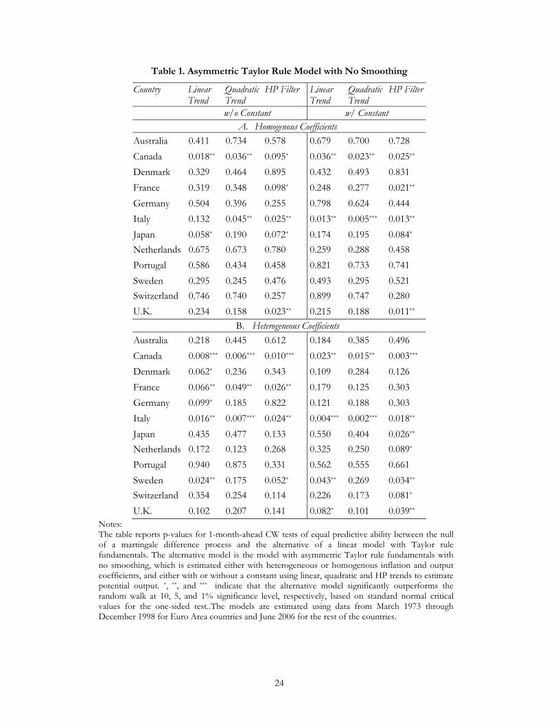
24

Table 1. Asymmetric Taylor Rule Model with No Smoothing

Country Linear Trend

Quadratic Trend

HP Filter Linear Trend

Quadratic Trend

HP Filter

w/o Constant w/ Constant

A. Homogenous Coefficients

Australia 0.411 0.734 0.578 0.679 0.700 0.728

Canada 0.018** 0.036** 0.095* 0.036** 0.023** 0.025**

Denmark 0.329 0.464 0.895 0.432 0.493 0.831

France 0.319 0.348 0.098* 0.248 0.277 0.021**

Germany 0.504 0.396 0.255 0.798 0.624 0.444

Italy 0.132 0.045** 0.025** 0.013** 0.005*** 0.013**

Japan 0.058* 0.190 0.072* 0.174 0.195 0.084*

Netherlands 0.675 0.673 0.780 0.259 0.288 0.458

Portugal 0.586 0.434 0.458 0.821 0.733 0.741

Sweden 0.295 0.245 0.476 0.493 0.295 0.521

Switzerland 0.746 0.740 0.257 0.899 0.747 0.280

U.K. 0.234 0.158 0.023** 0.215 0.188 0.011**

B. Heterogeneous Coefficients

Australia 0.218 0.445 0.612 0.184 0.385 0.496

Canada 0.008*** 0.006*** 0.010*** 0.023** 0.015** 0.003***

Denmark 0.062* 0.236 0.343 0.109 0.284 0.126

France 0.066** 0.049** 0.026** 0.179 0.125 0.303

Germany 0.099* 0.185 0.822 0.121 0.188 0.303

Italy 0.016** 0.007*** 0.024** 0.004*** 0.002*** 0.018**

Japan 0.435 0.477 0.133 0.550 0.404 0.026**

Netherlands 0.172 0.123 0.268 0.325 0.250 0.089*

Portugal 0.940 0.875 0.331 0.562 0.555 0.661

Sweden 0.024** 0.175 0.052* 0.043** 0.269 0.034**

Switzerland 0.354 0.254 0.114 0.226 0.173 0.081*

U.K. 0.102 0.207 0.141 0.082* 0.101 0.039**

Notes: The table reports p-values for 1-month-ahead CW tests of equal predictive ability between the null of a martingale difference process and the alternative of a linear model with Taylor rule fundamentals. The alternative model is the model with asymmetric Taylor rule fundamentals with no smoothing, which is estimated either with heterogeneous or homogenous inflation and output coefficients, and either with or without a constant using linear, quadratic and HP trends to estimate potential output. *, **, and *** indicate that the alternative model significantly outperforms the random walk at 10, 5, and 1% significance level, respectively, based on standard normal critical values for the one-sided test..The models are estimated using data from March 1973 through December 1998 for Euro Area countries and June 2006 for the rest of the countries.

25

Table 2. Asymmetric Taylor Rule Model with Smoothing

Country Linear Trend

Quadratic Trend

HP Filter Linear Trend

Quadratic Trend

HP Filter

w/o Constant w/ Constant

A. Homogenous Coefficients

Australia 0.171 0.244 0.192 0.103 0.143 0.169

Canada 0.028** 0.055* 0.178 0.086* 0.074** 0.028**

Denmark 0.209 0.281 0.505 0.440 0.452 0.635

France 0.040** 0.037** 0.010*** 0.080* 0.060* 0.013**

Germany 0.459 0.462 0.647 0.562 0.423 0.728

Italy 0.005*** 0.003*** 0.004*** 0.005*** 0.003*** 0.005***

Japan 0.012** 0.004*** 0.059* 0.029** 0.006*** 0.076*

Netherlands 0.262 0.271 0.285 0.142 0.153 0.216

Portugal 0.462 0.430 0.238 0.919 0.906 0.637

Sweden 0.824 0.744 0.818 0.852 0.836 0.820

Switzerland 0.277 0.202 0.134 0.283 0.150 0.161

U.K. 0.354 0.291 0.146 0.342 0.307 0.064*

B. Heterogeneous Coefficients

Australia 0.096* 0.151 0.174 0.054* 0.118 0.087*

Canada 0.011** 0.003*** 0.076* 0.042** 0.005*** 0.011**

Denmark 0.089* 0.187 0.059* 0.374 0.439 0.110

France 0.032** 0.027** 0.022** 0.195 0.125 0.056*

Germany 0.282 0.456 0.908 0.402 0.349 0.578

Italy 0.002*** 0.001*** 0.001*** 0.009*** 0.007*** 0.009***

Japan 0.016** 0.002*** 0.010*** 0.042** 0.005*** 0.004***

Netherlands 0.036** 0.016** 0.012** 0.156 0.083* 0.034**

Portugal 0.979 0.971 0.905 0.981 0.969 0.844

Sweden 0.718 0.861 0.496 0.882 0.919 0.773

Switzerland 0.173 0.147 0.055* 0.170 0.081* 0.032**

U.K. 0.172 0.280 0.176 0.108 0.095* 0.060*

Notes: The table reports p-values for 1-month-ahead CW tests of equal predictive ability between the null of a martingale difference process and the alternative of a linear model with Taylor rule fundamentals. The alternative model is the model with asymmetric Taylor rule fundamentals with smoothing, which is estimated either with heterogeneous or homogenous inflation and output coefficients, and either with or without a constant using linear, quadratic and HP trends to estimate potential output. *, **, and *** indicate that the alternative model significantly outperforms the random walk at 10, 5, and 1% significance level, respectively, based on standard normal critical values for the one-sided test. The models are estimated using data from March 1973 through December 1998 for Euro Area countries and June 2006 for the rest of the countries.

26

Table 3. Symmetric Taylor Rule Model with No Smoothing

Country Linear Trend

Quadratic Trend

HP Filter Linear Trend

Quadratic Trend

HP Filter

w/o Constant w/ Constant

A. Homogenous Coefficients

Australia 0.536 0.615 0.588 0.155 0.383 0.478

Canada 0.048** 0.019** 0.140 0.006*** 0.017** 0.025**

Denmark 0.381 0.371 0.772 0.325 0.462 0.915

France 0.174 0.852 0.234 0.406 0.447 0.152

Germany 0.591 0.599 0.400 0.555 0.412 0.210

Italy 0.098* 0.083* 0.025** 0.137 0.044** 0.026**

Japan 0.425 0.174 0.409 0.063* 0.198 0.076*

Netherlands 0.582 0.815 0.989 0.674 0.690 0.804

Portugal 0.945 0.724 0.893 0.516 0.379 0.411

Sweden 0.283 0.321 0.466 0.299 0.228 0.480

Switzerland 0.731 0.965 0.597 0.565 0.521 0.280

U.K. 0.460 0.468 0.030** 0.313 0.227 0.034**

B. Heterogeneous Coefficients

Australia 0.131 0.126 0.605 0.020** 0.140 0.328

Canada 0.003*** 0.006*** 0.003*** 0.003*** 0.003*** 0.002***

Denmark 0.113 0.473 0.779 0.050** 0.185 0.305

France 0.861 0.289 0.608 0.048** 0.033** 0.023**

Germany 0.350 0.057* 0.788 0.052* 0.041** 0.211

Italy 0.115 0.014** 0.057* 0.015** 0.005*** 0.020**

Japan 0.425 0.256 0.423 0.412 0.337 0.120

Netherlands 0.584 0.252 0.980 0.174 0.111 0.214

Portugal 0.736 0.574 0.064* 0.939 0.846 0.291

Sweden 0.114 0.198 0.271 0.020** 0.113 0.049**

Switzerland 0.552 0.264 0.510 0.129 0.078* 0.080*

U.K. 0.023** 0.051* 0.004*** 0.020** 0.036** 0.020**

Notes: The table reports p-values for 1-month-ahead CW tests of equal predictive ability between the null of a martingale difference process and the alternative of a linear model with Taylor rule fundamentals. The alternative model is the model with symmetric Taylor rule fundamentals with no smoothing, which is estimated either with heterogeneous or homogenous inflation and output coefficients, and either with or without a constant using linear, quadratic and HP trends to estimate potential output. *, **, and *** indicate that the alternative model significantly outperforms the random walk at 10, 5, and 1% significance level, respectively, based on standard normal critical values for the one-sided test. The models are estimated using data from January 1975 for Canada, September 1975 for Switzerland, January 1983 for Portugal, and March 1973 for the rest of the countries. The sample ends in November 2004 for Sweden, December 1998 for Euro Area countries and June 2006 for the rest of the countries.

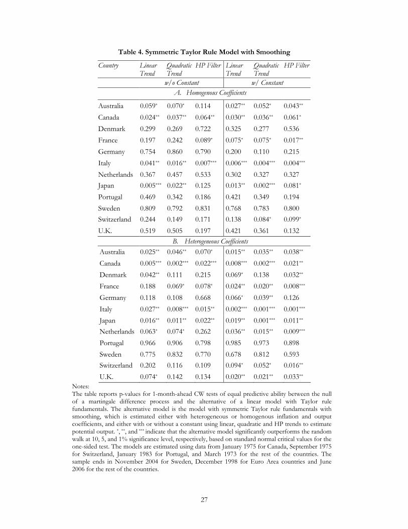
27

Table 4. Symmetric Taylor Rule Model with Smoothing

Country Linear Trend

Quadratic Trend

HP Filter Linear Trend

Quadratic Trend

HP Filter

w/o Constant w/ Constant

A. Homogenous Coefficients

Australia 0.059* 0.070* 0.114 0.027** 0.052* 0.043**

Canada 0.024** 0.037** 0.064** 0.030** 0.036** 0.061*

Denmark 0.299 0.269 0.722 0.325 0.277 0.536

France 0.197 0.242 0.089* 0.075* 0.075* 0.017**

Germany 0.754 0.860 0.790 0.200 0.110 0.215

Italy 0.041** 0.016** 0.007*** 0.006*** 0.004*** 0.004***

Netherlands 0.367 0.457 0.533 0.302 0.327 0.327

Japan 0.005*** 0.022** 0.125 0.013** 0.002*** 0.081*

Portugal 0.469 0.342 0.186 0.421 0.349 0.194

Sweden 0.809 0.792 0.831 0.768 0.783 0.800

Switzerland 0.244 0.149 0.171 0.138 0.084* 0.099*

U.K. 0.519 0.505 0.197 0.421 0.361 0.132

B. Heterogeneous Coefficients

Australia 0.025** 0.046** 0.070* 0.015** 0.035** 0.038**

Canada 0.005*** 0.002*** 0.022*** 0.008*** 0.002*** 0.021**

Denmark 0.042** 0.111 0.215 0.069* 0.138 0.032**

France 0.188 0.069* 0.078* 0.024** 0.020** 0.008***

Germany 0.118 0.108 0.668 0.066* 0.039** 0.126

Italy 0.027** 0.008*** 0.015** 0.002*** 0.001*** 0.001***

Japan 0.016** 0.011** 0.022** 0.019** 0.001*** 0.011**

Netherlands 0.063* 0.074* 0.262 0.036** 0.015** 0.009***

Portugal 0.966 0.906 0.798 0.985 0.973 0.898

Sweden 0.775 0.832 0.770 0.678 0.812 0.593

Switzerland 0.202 0.116 0.109 0.094* 0.052* 0.016**

U.K. 0.074* 0.142 0.134 0.020** 0.021** 0.033**

Notes: The table reports p-values for 1-month-ahead CW tests of equal predictive ability between the null of a martingale difference process and the alternative of a linear model with Taylor rule fundamentals. The alternative model is the model with symmetric Taylor rule fundamentals with smoothing, which is estimated either with heterogeneous or homogenous inflation and output coefficients, and either with or without a constant using linear, quadratic and HP trends to estimate potential output. *, **, and *** indicate that the alternative model significantly outperforms the random walk at 10, 5, and 1% significance level, respectively, based on standard normal critical values for the one-sided test. The models are estimated using data from January 1975 for Canada, September 1975 for Switzerland, January 1983 for Portugal, and March 1973 for the rest of the countries. The sample ends in November 2004 for Sweden, December 1998 for Euro Area countries and June 2006 for the rest of the countries.

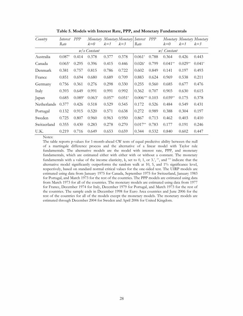
28

Table 5. Models with Interest Rate, PPP, and Monetary Fundamentals

Country Interest Rate

PPP Monetary k=0

Monetary k=1

Monetary k=3

Interest Rate

PPP Monetary k=0

Monetary k=1

Monetary k=3

w/o Constant w/ Constant

Australia 0.087* 0.414 0.378 0.377 0.378 0.061* 0.788 0.364 0.426 0.443

Canada 0.065* 0.295 0.396 0.415 0.446 0.026* 0.799 0.041** 0.029** 0.041*

Denmark 0.381 0.757 0.815 0.786 0.722 0.602 0.849 0.141 0.197 0.493

France 0.851 0.694 0.680 0.689 0.709 0.883 0.624 0.969 0.538 0.211

Germany 0.756 0.361 0.276 0.298 0.330 0.255 0.560 0.685 0.677 0.476

Italy 0.393 0.649 0.991 0.991 0.992 0.362 0.707 0.903 0.630 0.615

Japan 0.685 0.089* 0.063* 0.057* 0.051* 0.006*** 0.103 0.039** 0.175 0.378

Netherlands 0.377 0.426 0.518 0.529 0.545 0.172 0.526 0.484 0.549 0.431

Portugal 0.132 0.915 0.520 0.571 0.638 0.272 0.989 0.388 0.304 0.197

Sweden 0.725 0.807 0.960 0.963 0.950 0.867 0.713 0.462 0.403 0.410

Switzerland 0.355 0.430 0.283 0.278 0.270 0.017** 0.783 0.177 0.191 0.246

U.K. 0.219 0.716 0.649 0.653 0.659 0.344 0.532 0.840 0.602 0.447

Notes: The table reports p-values for 1-month-ahead CW tests of equal predictive ability between the null of a martingale difference process and the alternative of a linear model with Taylor rule fundamentals. The alternative models are the model with interest rate, PPP, and monetary fundamentals, which are estimated either with either with or without a constant. The monetary

fundamentals with a value of the income elasticity, k, set to 0, 1, or 3.*, **, and *** indicate that the alternative model significantly outperforms the random walk at 10, 5, and 1% significance level, respectively, based on standard normal critical values for the one-sided test. The UIRP models are estimated using data from January 1975 for Canada, September 1975 for Switzerland, January 1983 for Portugal, and March 1973 for the rest of the countries. The PPP models are estimated using data from March 1973 for all of the countries. The monetary models are estimated using data from 1977 for France, December 1974 for Italy, December 1979 for Portugal, and March 1973 for the rest of the countries. The sample ends in December 1998 for Euro Area countries and June 2006 for the rest of the countries for all of the models except the monetary models. The monetary models are estimated through December 2004 for Sweden and April 2006 for United Kingdom.

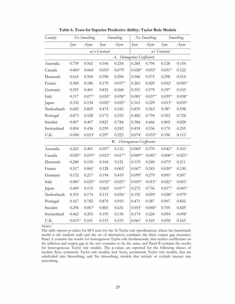
29

Table 6. Tests for Superior Predictive Ability: Taylor Rule Models

Country No Smoothing Smoothing No Smoothing Smoothing

Sym Asym Sym Asym Sym Asym Sym Asym

w/o Constant w/ Constant

A. Homogenous Coefficients

Australia 0.739 0.562 0.106 0.234 0.285 0.794 0.128 0.154

Canada 0.069* 0.064* 0.055* 0.079* 0.028** 0.055* 0.031** 0.122

Denmark 0.616 0.504 0.398 0.294 0.506 0.575 0.298 0.514

France 0.369 0.186 0.170 0.037** 0.265 0.429 0.052* 0.050**

Germany 0.591 0.401 0.835 0.568 0.351 0.579 0.197 0.535

Italy 0.117 0.077* 0.035** 0.038** 0.081* 0.037** 0.039** 0.038**

Japan 0.332 0.154 0.025** 0.025** 0.163 0.229 0.013** 0.035**

Netherlands 0.683 0.829 0.474 0.343 0.835 0.363 0.387 0.198

Portugal 0.873 0.528 0.173 0.325 0.482 0.794 0.353 0.724

Sweden 0.497 0.407 0.821 0.784 0.384 0.466 0.805 0.828

Switzerland 0.854 0.436 0.259 0.242 0.418 0.536 0.170 0.255

U.K. 0.096* 0.053* 0.297 0.222 0.074* 0.033** 0.196 0.113

B. Heterogeneous Coefficients

Australia 0.263 0.401 0.057* 0.152 0.069* 0.370 0.042** 0.103

Canada 0.020** 0.019** 0.012** 0.017** 0.009*** 0.045** 0.008*** 0.025**

Denmark 0.280 0.150 0.104 0.121 0.119 0.240 0.075* 0.211

France 0.517 0.061* 0.128 0.065* 0.067* 0.243 0.030** 0.130

Germany 0.132 0.217 0.194 0.419 0.099* 0.279 0.091* 0.507

Italy 0.081* 0.025** 0.032** 0.023** 0.019** 0.015** 0.022** 0.053*

Japan 0.469 0.115 0.062* 0.017** 0.272 0.736 0.017** 0.043**

Netherlands 0.353 0.174 0.113 0.036** 0.192 0.095* 0.028** 0.079*

Portugal 0.167 0.782 0.870 0.910 0.471 0.587 0.907 0.856

Sweden 0.296 0.067* 0.803 0.631 0.053* 0.048** 0.705 0.829

Switzerland 0.462 0.205 0.195 0.130 0.174 0.224 0.054* 0.098*

U.K. 0.015** 0.101 0.153 0.333 0.061* 0.165 0.058* 0.165

Notes: The table reports p-values for SPA tests for the 16 Taylor rule specifications, where the benchmark model is the random walk and the set of alternatives combines the three output gap measures. Panel A contains the results for homogenous Taylor rule fundamentals, that restrict coefficients on the inflation and output gap in the two countries to be the same, and Panel B contains the results for heterogeneous Taylor rule models. The p-values are reported for the following classes of models: Sym, symmetric Taylor rule models, and Asym, asymmetric Taylor rule models, that are subdivided into Smoothing, and No Smoothing, models that include or exclude interest rate smoothing.

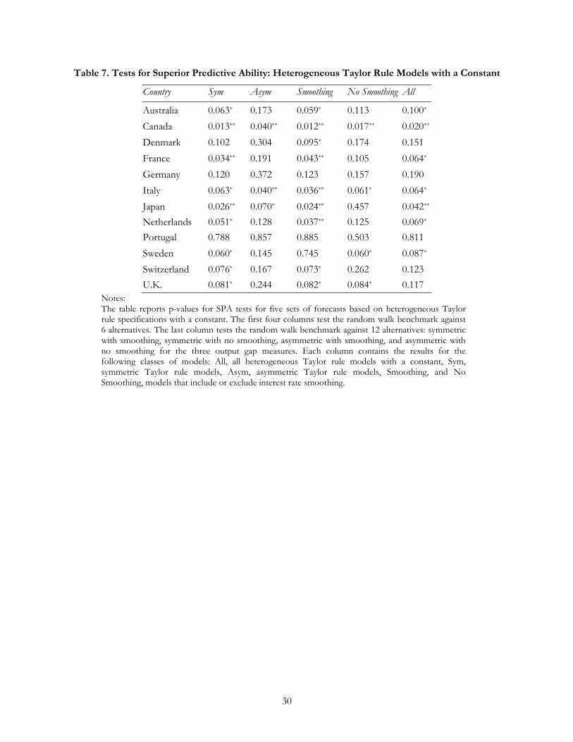
30

Table 7. Tests for Superior Predictive Ability: Heterogeneous Taylor Rule Models with a Constant

Country Sym Asym Smoothing No Smoothing All

Australia 0.063* 0.173 0.059* 0.113 0.100*

Canada 0.013** 0.040** 0.012** 0.017** 0.020**

Denmark 0.102 0.304 0.095* 0.174 0.151

France 0.034** 0.191 0.043** 0.105 0.064*

Germany 0.120 0.372 0.123 0.157 0.190

Italy 0.063* 0.040** 0.036** 0.061* 0.064*

Japan 0.026** 0.070* 0.024** 0.457 0.042**

Netherlands 0.051* 0.128 0.037** 0.125 0.069*

Portugal 0.788 0.857 0.885 0.503 0.811

Sweden 0.060* 0.145 0.745 0.060* 0.087*

Switzerland 0.076* 0.167 0.073* 0.262 0.123

U.K. 0.081* 0.244 0.082* 0.084* 0.117

Notes: The table reports p-values for SPA tests for five sets of forecasts based on heterogeneous Taylor rule specifications with a constant. The first four columns test the random walk benchmark against 6 alternatives. The last column tests the random walk benchmark against 12 alternatives: symmetric with smoothing, symmetric with no smoothing, asymmetric with smoothing, and asymmetric with no smoothing for the three output gap measures. Each column contains the results for the following classes of models: All, all heterogeneous Taylor rule models with a constant, Sym, symmetric Taylor rule models, Asym, asymmetric Taylor rule models, Smoothing, and No Smoothing, models that include or exclude interest rate smoothing.

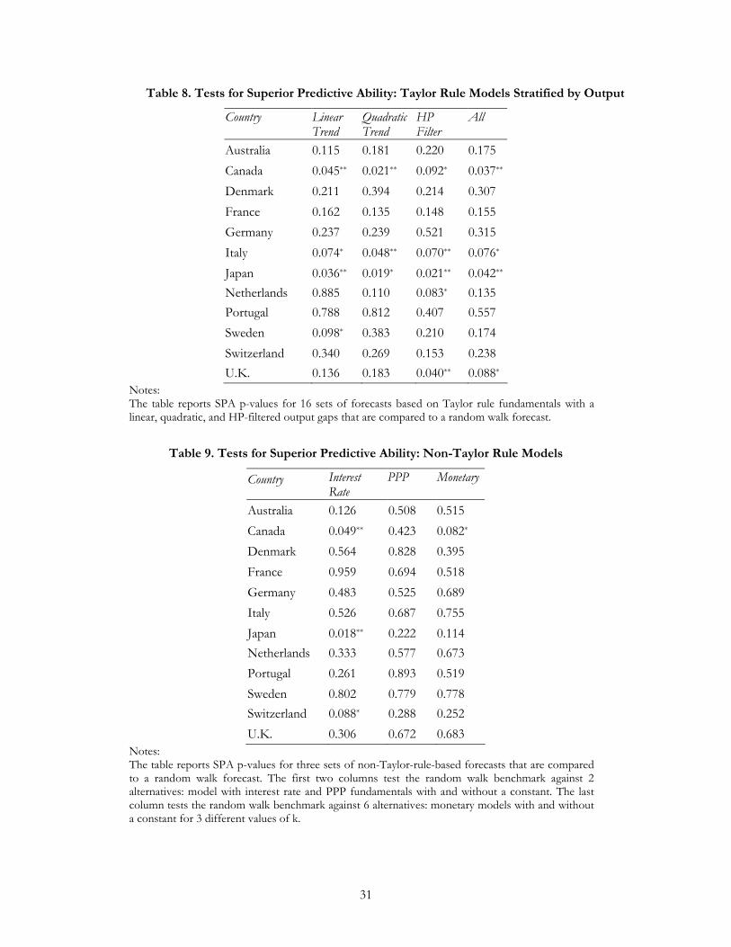
31

Table 8. Tests for Superior Predictive Ability: Taylor Rule Models Stratified by Output

Country Linear Trend

Quadratic Trend

HP Filter

All

Australia 0.115 0.181 0.220 0.175

Canada 0.045** 0.021** 0.092* 0.037**

Denmark 0.211 0.394 0.214 0.307

France 0.162 0.135 0.148 0.155

Germany 0.237 0.239 0.521 0.315

Italy 0.074* 0.048** 0.070** 0.076*

Japan 0.036** 0.019* 0.021** 0.042**

Netherlands 0.885 0.110 0.083* 0.135

Portugal 0.788 0.812 0.407 0.557

Sweden 0.098* 0.383 0.210 0.174

Switzerland 0.340 0.269 0.153 0.238

U.K. 0.136 0.183 0.040** 0.088*

Notes: The table reports SPA p-values for 16 sets of forecasts based on Taylor rule fundamentals with a linear, quadratic, and HP-filtered output gaps that are compared to a random walk forecast.

Table 9. Tests for Superior Predictive Ability: Non-Taylor Rule Models

Country Interest Rate

PPP Monetary

Australia 0.126 0.508 0.515

Canada 0.049** 0.423 0.082*

Denmark 0.564 0.828 0.395

France 0.959 0.694 0.518

Germany 0.483 0.525 0.689

Italy 0.526 0.687 0.755

Japan 0.018** 0.222 0.114

Netherlands 0.333 0.577 0.673

Portugal 0.261 0.893 0.519

Sweden 0.802 0.779 0.778

Switzerland 0.088* 0.288 0.252

U.K. 0.306 0.672 0.683

Notes: The table reports SPA p-values for three sets of non-Taylor-rule-based forecasts that are compared to a random walk forecast. The first two columns test the random walk benchmark against 2 alternatives: model with interest rate and PPP fundamentals with and without a constant. The last column tests the random walk benchmark against 6 alternatives: monetary models with and without a constant for 3 different values of k.

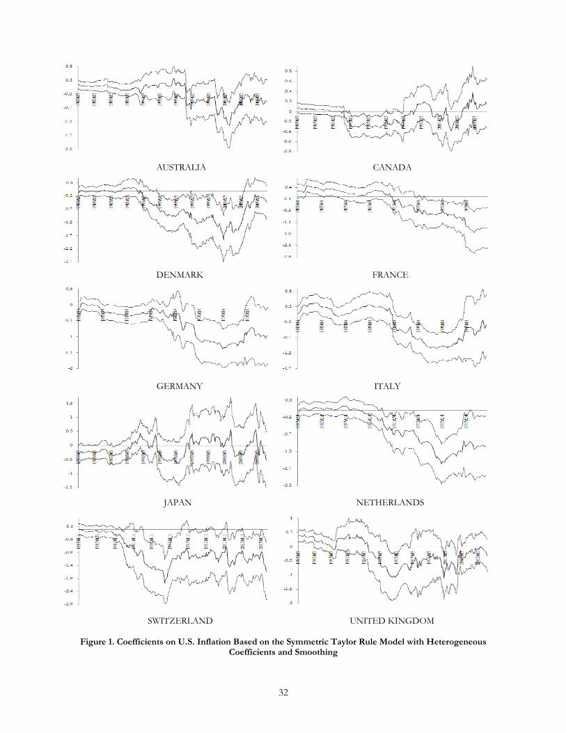
32

AUSTRALIA CANADA

DENMARK FRANCE

GERMANY ITALY

JAPAN NETHERLANDS

SWITZERLAND UNITED KINGDOM

Figure 1. Coefficients on U.S. Inflation Based on the Symmetric Taylor Rule Model with Heterogeneous Coefficients and Smoothing

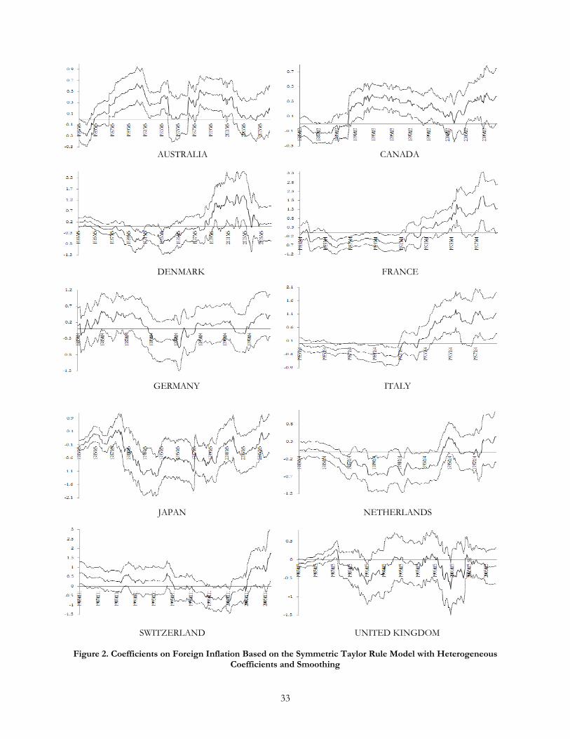
33

AUSTRALIA CANADA

DENMARK FRANCE

GERMANY ITALY

JAPAN NETHERLANDS

SWITZERLAND UNITED KINGDOM Figure 2. Coefficients on Foreign Inflation Based on the Symmetric Taylor Rule Model with Heterogeneous

Coefficients and Smoothing